Numerical Analysis and Scientific Computing

Preprint Seria

A Study of Self-Propelled Elastic

Cylindrical Micro-swimmers using

Modeling and Computation

L. Shi S. Canic A. Quaini T.-W. Pan

Preprint #42

Department of Mathematics

University of Houston

October 2015

A Study of Self-Propelled Elastic Cylindrical Micro-swimmers

using Modeling and Computation

Lingling Shi

a

, Suncica

ˇ

Canic

,a, Annalisa Quaini

a

, Tsorng-Whay Pan

a

aDepartment of Mathematics, University of Houston, 4800 Calhoun Rd, Houston TX 77204, USA

Abstract

We study propulsion of micro swimmers in 3D creeping flow. The swimmers are assumed to be madeof elastic cylindrical hollow tubes. The swimming is generated by the contractions of the tube’s elasticmembrane walls producing a traveling wave in the form of a “step-function” traversing the swimmerfrom right to left, propelling the swimmer from left to right. The problem is motivated by medicalapplications such as drug delivery. The influence of several non-dimensional design parameters on thevelocity of the swimmer is investigated, including the swimmer aspect ratio, and the amplitude of thetraveling wave relative to the swimmer radius. An immersed boundary method based on a finite elementmethod approach is successfully combined with an elastic spring network model to simulate the two-wayfluid-structure interaction coupling between the elastic cylindrical tube and the flow of a 3D viscous,incompressible fluid. To gain a deeper insight into the influence of various parameters on the swimmerspeed, a reduced 1D fluid-structure interaction model was derived and validated. It was found that fastswimmers are those with large tube aspect ratios, and with the amplitude of the traveling wave which isroughly 50% of the reference swimmer radius. It was shown that the speed of our “optimal swimmer”is around 1.5 swimmer lengths per second, which is at the top of the class of all currently manufacturedmicro-swimmers swimming in low Reynolds number flows (Re = 106), reported in [11].

Keywords Micro-swimmers, Immersed boundary method, Fluid-structure interaction, Reduced 1Dmodel.

1. Introduction

Micro robots, or micro swimmers, are a class of artificial nano- or micro-scale particles capable of

converting external energy into motion. They swim in low Reynolds number regimes (Re = 106)

where viscosity dominates. Due to the reversibility in low Reynolds number flow (e.g. Stokes flow)

the action of swimming micro organisms in nature are di↵erent from regular size swimmers such as fish

[30]. New propulsion methodologies are needed to eciently move these swimmers. It turns out that all

the micro-swimming organisms create in one way or another a traveling wave, moving in the opposite

direction of the swimmer motion (see e.g., spermatozoa [5, 24], celia [19], amoeba [3], and anguilliform

swimmers [14, 28]). Such a traveling wave can be artificially generated in synthetic swimmers by using,

e.g., piezoelectric [16], ICFP [13], or magnetic actuators [9, 31, 17]. Applications of such micro-swimmers

include biomedical applications such as drug delivery (“smart pills” [10]) and diagnostic tools. Biological

low Reynolds number flow regimes can be found in, for example, blood flow in arterioles and in capillary

beds, which populate all of our organs, in mammalian productive systems [4], and in intestines [26]. A

comprehensive review of the literature on manufactured mili and micro medical swimmers can be found

in [11].

Corresponding authorEmail addresses: shi@math.uh.edu (Lingling Shi), canic@math.uh.edu (Suncica Canic), quaini@math.uh.edu

(Annalisa Quaini), pan@math.uh.edu (Tsorng-Whay Pan)

Preprint submitted to Elsevier September 6, 2015

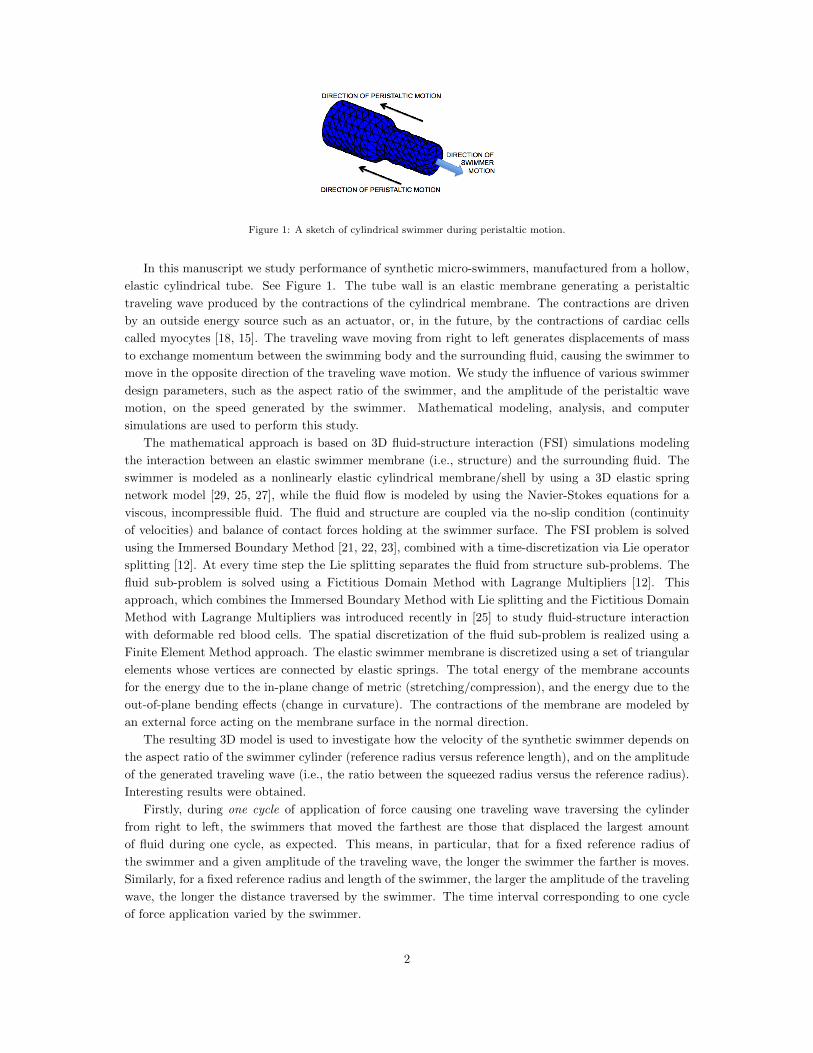
Figure 1: A sketch of cylindrical swimmer during peristaltic motion.

In this manuscript we study performance of synthetic micro-swimmers, manufactured from a hollow,

elastic cylindrical tube. See Figure 1. The tube wall is an elastic membrane generating a peristaltic

traveling wave produced by the contractions of the cylindrical membrane. The contractions are driven

by an outside energy source such as an actuator, or, in the future, by the contractions of cardiac cells

called myocytes [18, 15]. The traveling wave moving from right to left generates displacements of mass

to exchange momentum between the swimming body and the surrounding fluid, causing the swimmer to

move in the opposite direction of the traveling wave motion. We study the influence of various swimmer

design parameters, such as the aspect ratio of the swimmer, and the amplitude of the peristaltic wave

motion, on the speed generated by the swimmer. Mathematical modeling, analysis, and computer

simulations are used to perform this study.

The mathematical approach is based on 3D fluid-structure interaction (FSI) simulations modeling

the interaction between an elastic swimmer membrane (i.e., structure) and the surrounding fluid. The

swimmer is modeled as a nonlinearly elastic cylindrical membrane/shell by using a 3D elastic spring

network model [29, 25, 27], while the fluid flow is modeled by using the Navier-Stokes equations for a

viscous, incompressible fluid. The fluid and structure are coupled via the no-slip condition (continuity

of velocities) and balance of contact forces holding at the swimmer surface. The FSI problem is solved

using the Immersed Boundary Method [21, 22, 23], combined with a time-discretization via Lie operator

splitting [12]. At every time step the Lie splitting separates the fluid from structure sub-problems. The

fluid sub-problem is solved using a Fictitious Domain Method with Lagrange Multipliers [12]. This

approach, which combines the Immersed Boundary Method with Lie splitting and the Fictitious Domain

Method with Lagrange Multipliers was introduced recently in [25] to study fluid-structure interaction

with deformable red blood cells. The spatial discretization of the fluid sub-problem is realized using a

Finite Element Method approach. The elastic swimmer membrane is discretized using a set of triangular

elements whose vertices are connected by elastic springs. The total energy of the membrane accounts

for the energy due to the in-plane change of metric (stretching/compression), and the energy due to the

out-of-plane bending e↵ects (change in curvature). The contractions of the membrane are modeled by

an external force acting on the membrane surface in the normal direction.

The resulting 3D model is used to investigate how the velocity of the synthetic swimmer depends on

the aspect ratio of the swimmer cylinder (reference radius versus reference length), and on the amplitude

of the generated traveling wave (i.e., the ratio between the squeezed radius versus the reference radius).

Interesting results were obtained.

Firstly, during one cycle of application of force causing one traveling wave traversing the cylinder

from right to left, the swimmers that moved the farthest are those that displaced the largest amount

of fluid during one cycle, as expected. This means, in particular, that for a fixed reference radius of

the swimmer and a given amplitude of the traveling wave, the longer the swimmer the farther is moves.

Similarly, for a fixed reference radius and length of the swimmer, the larger the amplitude of the traveling

wave, the longer the distance traversed by the swimmer. The time interval corresponding to one cycle

of force application varied by the swimmer.

2

However, when multiple cycles of force application were considered during a fixed time interval,

di↵erent results were obtained. In terms of the aspect ratio, short swimmers, i.e., the swimmers with

large aspect ratios, moved the farthest within a given time interval. We found that such swimmers have

the largest average velocity per one cycle, as they produce the largest rate of change of displaced mass

per unit time.

In terms of the traveling wave amplitude, the swimmers experiencing roughly 50% of radius displace-

ment moved the farthest within a given time interval. We found, again, that such a swimmers have the

largest average velocity in one cycle.

Thus, fast swimmers are those with large aspect ratios whose radius deforms roughly 50% in each

cycle. Such swimmers are capable of generating a large number of contractions per unit time because of

their short length, producing the largest rate of change of displaced mass per unit time.

To get a better insight into the influence of di↵erent parameters on the velocity of the swimmers,

we developed a nonlinear 1D reduced model of fluid-structure interaction between a slender (linear)

swimmer and the flow of a creeping fluid. A similar 1D model was also considered in [2] for a spherical

swimmer with internally generated traveling waves. We show that the reduced model approximates well

our 3D FSI simulations of slender swimmers that deform up to 50% of the reference radius.

Finally, we show that our fastest swimmers travel 1.5 swimmer lengths per second, which is near the

top of the class of all currently available manufactured artificial swimmers swimming and low Reynolds

numbers. More precisely, in a recent review article [11] it was reported that at Reynolds numbers of

106, which is our flow regime, the currently manufactured artificial swimmers typically swim at the

speed between 0.6 swimmer lengths per second (15-Au/Ni/Au/Pt-CNT motor with 4.3 µm diameter

cargo), and 2 swimmer lengths per second (striped metallic nano rod). Thus, our results appear to be

quite relevant, and are a first step in our long-term goal to produce cylindrical medical micro-swimmers

driven by the contractions of cardiac myocytes [15, 18].

2. Problem description, mathematical model, and numerical solver

2.1. Problem Description

We study propulsion of an elastic cylindrical (hollow) tube by a peristaltic motion of its elastic

membrane walls, moving through a viscous, incompressible fluid at low Reynolds numbers. The elastic

cylindrical membrane is immersed in the fluid occupying a larger cylinder with rigid walls, whose radius

is much larger than that of the swimmer so that it does not influence the swimmer motion. The reference

configuration of the swimmer is a straight cylinder of radius R0

and length L. A traveling wave moving

from right to left is induced in the cylinder membrane, see Figure 1, producing an overall motion of

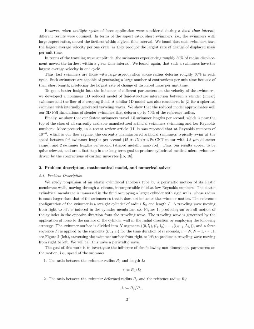
the cylinder in the opposite direction from the traveling wave. The traveling wave is generated by the

application of force to the surface of the cylinder wall in the radial direction by employing the following

strategy. The swimmer surface is divided into N segments ((0, l1

), (l1

, l2

), · · · , (lN1

, LN

)), and a force

sequence Fi

is applied to the segments (li1

, li

) for the time duration of ti

seconds, i = N,N 1, · · · , 1,see Figure 2 (left), traversing the swimmer surface from right to left to produce a traveling wave moving

from right to left. We will call this wave a peristaltic wave.

The goal of this work is to investigate the influence of the following non-dimensional parameters on

the motion, i.e., speed of the swimmer:

1. The ratio between the swimmer radius R0

and length L:

:= R0

/L;

2. The ratio between the swimmer deformed radius Rf

and the reference radius R0

:

:= Rf

/R0

,

3

γ

ω

Ω

Γ

z

y x

Figure 2: Left: A sketch of force application strategy. Right: Computational domain with elastic swimmer.

i.e., the relative amplitude of the peristaltic wave.

Related to the velocity is the distance traveled by the swimmer. We will investigate the distance traveled

by the swimmer during:

• One peristaltic contraction of the swimmer, i.e., one cycle of force application (the time interval is

not fixed; it depends on the swimmer); and

• Multiple peristaltic contractions of the swimmer (during a fixed time interval).

The results are not as straight-forward as one might expect. They are influenced by the amount of

displaced mass, the rate of change of displaced mass, the nonlinearity of the swimmer model, the fluid

viscosity, and by the “added mass e↵ect” associated with the displaced fluid during swimmer contractions.

We remark here that one way to introduce a peristaltic motion of the swimmer would have been to

impose the location of the swimmer membrane a priori, prescribing the peristaltic wave independently

of the fluid surrounding the swimmer. This would have been a much easier task to study from both the

mathematical and computational points of view, since this approach defines a fluid-structure interaction

problem with one-way coupling due to the prescribed structure motion. In practice, however, peristaltic

motion of the swimmer is produced by the action of a certain force on the swimmer surface, which gives

rise to a fluid-structure interaction problem with two-way coupling between the fluid and structure. It

turns out that to produce a peristaltic way for such a swimmer immersed in the fluid is a non-trivial task,

since the swimmer deformation and its motion depend nonlinearly not only on the elastic properties of

the swimmer membrane, but also on the fluid stress exerted by the fluid onto the swimmer. Our results,

presented below, suggest a practical strategy of application of force onto the swimmer surface to produce

a desired peristaltic swimmer motion, which may be adopted in the design of an actual swimmer.

2.2. Mathematical Model

The mathematical problem is that of fluid-structure interaction between an incompressible, viscous

fluid, and elastic cylinder immersed in the fluid. The numerical approach to solve this fluid-structure

interaction problem in this work is based on the Immersed Boundary Method coupled with the Fictitious

Domain Method with Lagrange Multipliers to solve the corresponding fluid sub-problem. The general

mathematical framework of the problem is given in the context of the Immersed Boundary Method

formulation (IBM).

We begin by defining the fluid and structure models, and then define the coupled fluid-structure

interaction problem in the context of IBM.

4

The fluid model. The fluid motion will be modeled by the time-dependent Stokes (Navier-Stokes)

equations for an incompressible, viscous fluid defined inside a large cylindrical “fluid container”, which we

denote by !. See Figure 2 (right). Since our 3D methodology works for the full Navier-Stokes equations,

we present the model problem for the Navier-Stokes equations and then indicate how simplifications of

the problem can be done to solve the time-dependent Stokes problem. The Navier-Stokes equations,

defined on a time interval (0, T ), T > 0, read as follows:

@u

@t+ u ·ru

= r + f in ! (0, T ), (1)

r · u = 0 in ! (0, T ). (2)

Here u is the fluid velocity, is the fluid density, f is the body force, and = pI + 2µD(u) is the

fluid Cauchy stress tensor for Newtonian fluids, where p is the fluid pressure, µ is the kinematic viscosity

coecient, and D(u) = 1

2

(ru+r

u) is the symmetrized gradient of u.

For low Reynolds number flows the convection term u ·ru is small and can be neglected, giving rise

to the time-dependent (linear) Stokes equations. This will be the case with our swimmer.

Equations (1) and (2) are supplemented with the no-slip boundary condition on the boundary of

!, and an initial condition u

0

for the fluid velocity, which we normally take to be equal to zero:

u = 0 on (0, T ), (3)

u(x, 0) = u

0

(x) in !. (4)

The elastic swimmer model. We will be assuming that our elastic swimmer behaves as a (non-

linearly) elastic membrane/shell. The model that we present below will be of the form

mr F(r) = F

ext, (5)

where m is the mass density of the swimmer, r is a vector describing the location of points of the

swimmer, F is the force due to the elastic and bending energy of the swimmer, Fext is the external force

density, and ˙( ) denotes the time derivative. The term F(r) will be obtained as the derivative of the

energy density with respect to r, where the energy density will account for the energy due to the in-plane

change of metric due to stretching/compression (membrane e↵ects), and the energy associated with the

change in curvature due to the out-of-plane bending e↵ects (shell e↵ects). These ideas are incorporated

Figure 3: Swimmer membrane discretization using elastic springs.

into a three–dimensional elastic spring network, developed and used in [29, 25, 27]. Based on this model,

the (middle surface of the) swimmer membrane/shell can be viewed as a collection of small triangular

elements whose vertices are connected by springs, as shown in Figure 3. The total number of vertices

(nodes) will be denoted by Nn

, while the total number of springs by Ns

. The elastic energy of the

swimmer membrane/shell includes the energy stored due to the change of the length Ll

of each spring

with respect to its reference length L0

l

, and the energy stored due to the change in the angle l

between

two neighboring triangular elements. Thus, the elastic energy of the swimmer membrane

E = Ee

+ Eb

(6)

5

is the sum of the total energy due to stretch/compression

Ee

=ks

2

NsX

l=1

(Ll

L0

l

)2, (7)

and the total energy due to bending

Eb

=kb

2

NsX

l=1

Ll

tan2(l

2). (8)

Here ks

and kb

are the spring constants accounting for the changes in length and bending angle, respec-

tively, and l

is the angle between the normal outer vectors of the two neighboring triangular elements,

which have the side l as their boundary. In equation (8) the tangent function was chosen to avoid the

folding of springs at large bending deformations.

We note that in [29, 25, 27] additional terms were considered in the definition of the elastic energy of

the membrane to enforce the local and global area conservation. This was done because in those works

the focus was on modeling the elastic properties of red blood cells. These additional terms are related

to the incompressibility of the membrane material, and to the total volume conservation within a cell,

which we do not have in our problem. In our model we dropped the area conservation property to be

able to capture, more realistically, the traveling wave in our swimmer membrane/shell.

To describe the elastodynamics of the swimmer we assign to each node (apex) i of the triangular

elements the position vector r

i

. Using vector analysis, the right hand-side of the energy function (6)

can be written as a function of ri

. Based on the principle of virtual work, the force acting on the ith

membrane node due to the elastic energy is then given by

F

i

= @E

@ri

, (9)

where F

i

= F

i

(r1

, . . . , rNn). We will be assuming that the swimmer membrane has a certain mass,

so that each node i is assigned mass m such that the total mass is equal to mNn

. If we assume that

external force F

ext is applied to the swimmer so that at each node the external force equals Fext

i

, then

each swimmer node moves based on the following equation of motion:

mr

i

F

i

= F

ext

i

. (10)

External force F

ext

i

in this FSI problem will include the force exerted by the fluid onto the structure,

i.e., the force that the structure feels from the fluid, given in Lagrangian coordinates by F

i

, and the

force F

e

i

exerted by other external sources such as, e.g., the actuators, causing the swimmer membrane

to contract to produce a traveling wave responsible for the peristaltic motion of the swimmer. Thus,

mr

i

F

i

= F

i

+ F

e

i

. (11)

The position r

i

of the ith membrane node is solved by discretizing equation (11) via a second order finite

di↵erence method.

The fluid-structure coupling. The fluid and structure are coupled via two coupling conditions at

the fluid-structure interface: (1) continuity of velocity, i.e., the no-slip condition, (Kinematic Coupling

Condition), and (2) balance of forces (Dynamic Coupling Condition). Namely, the balance of forces

imposed via the second Newton’s law of motion says that the elastodynamics of the fluid-structure

interface is driven by the jump in the normal fluid stress across the interface and the external forces

acting on the interface.

More precisely, if denotes the swimmer membrane, and F denotes the contact force that the

structure feels exerted by the fluid onto the structure (in Lagrangian coordinates), see equation (11),

and F

e denotes the external force on the structure that produces peristaltic wave motion, then the two

coupling conditions read:

6

• No-slip: dr/dt = u|

,

• Balance of forces: (fJ) |

= F = mr+F(r)+F

e, where f is the jump in the normal component

of the fluid stress (given in Eulerian coordinates), and J is the Jacobian of the transformation from

Eulerian to Lagrangian coordinates.

We do not need to specify (fJ) |

explicitly here because, in the Immersed Boundary Formulation, the

conversion from Eulerian to Lagrangian coordinates is done via integral formulations involving the Dirac

delta function, as we present below.

The Immersed Boundary Method (IBM) formulation of the coupled FSI problem. The

immersed boundary method, developed by Peskin, see e.g., [21, 22, 23], is employed in our study because

of its distinguishing features in dealing with the problem of fluid flow interacting with a flexible fluid–

structure interface immersed in the fluid. To write the IBM formulation of the problem we denote by

(q, r, s) the (Lagrangian) curvilinear coordinates associated with the structure, and introduce X(q; r; s; t)

to be the Cartesian coordinates at time t of the material point whose label is (q; r; s). Furthermore, let

m(q, r, s) denote the mass density of the material in the sense thatR

m(q, r, s) dq dr ds is the mass of

the part of the material defined by (q, r, s) 2 . Introduce (x) to denote the three-dimensional Delta

function (x1

)(x2

)(x3

), where x1

, x2

, x3

are the Cartesian components of x. Then the IBM formulation

of our FSI problem reads:

@u

@t+ u ·ru

= rp+ µu+ f , (12)

r · u = 0, (13)

f(x, t) =

ZF(q, r, s, t)(xX(q, r, s, t)) dqdrds, (14)

dX

dt= U(X(q, r, s, t), t) =

Zu(x, t)(xX(q, r, s, t))dx, (15)

where

F = mX+ F(X) + F

e. (16)

Notice that in this formulation the conversion from Eulerian to the Lagrangian coordinates is done via

the integral formulations (13) and (14) and so no explicit calculation of the Jacobian of the transformation

J is necessary. The fluid equations (12) and (13) are written entirely in the Eulerian form, while the

structure equation (16) is written entirely in the Lagrangian formulation. The influence of the structure

onto the fluid is included as an external force in the fluid equation (12), while the influence of the fluid

onto the structure is felt via the no-slip condition (15).

2.3. Numerical Solver

We implemented the Immersed Boundary Method to resolve the fluid-structure interaction, and the

Fictitious Domain Method to solve the fluid equations. Lagrange multipliers were employed to enforce

the incompressibility condition and the no-slip condition at the outer, rigid cylinder wall. This approach

was recently developed in [25] for the simulation of red blood cells interacting with an incompressible,

viscous, Newtonian fluid in a straight cylindrical tube with rigid walls.

The problem is numerically semi-discretized in time using the time discretization via Lie operator

splitting. This approach separates the entire FSI problem into “modules”, which can easily be modified

or dropped if necessary. For example, the advection module is simply ignored (dropped) in the case

of Stokes flow without any additional modifications in the fluid solver. The time-discretization via Lie

splitting for our Navier-Stokes FSI problem has 4 modules. The scheme starts by considering a certain

7

given velocity and structure position (from the previous time step). In the first module this given fluid

flow from the previous time step is modified to enforce the incompressibility condition by solving a

degenerate quasi-Stokes problem, see (26). In the second step, this new fluid velocity is used to calculate

the new location of the structure by enforcing the no-slip condition (the kinematic coupling condition

(15)), i.e., by updating the velocity of the swimmer to be equal to the velocity of the fluid from where the

new location of the swimmer is calculated. In this second step, the force exerted by the swimmer onto

the fluid (16) is also calculated and used in the next step to solve the momentum equation (12) for the

fluid problem, which includes the dynamic coupling condition (14) via force f that the fluid feels from

the structure. In the last step, the momentum equation (12) for the fluid flow is solved. To separate

between the advection and di↵usion e↵ects in the fluid problem, this last step is split into two modules:

the advection module, see equation (28), and the di↵usion module, see (29). The advection module can

easily be dropped when the Stokes, instead of the Navier-Stokes problem is solved, which is the case with

our low-Reynolds number swimmer. The result of these 4 modules is the updated fluid velocity, fluid

pressure, and the position of the immersed swimmer during one time step.

The spatial discretization associated with the Immersed Boundary Method formulation (12)-(16)

usually incorporates two spatial grids, one for the Eulerian (fluid) variables, and one for the Lagrangian

(structure) variables. The Eulerian grid will be based on the finite element method discretization of the

fluid domain, which we discuss in more detail below. At this point we specify that we will be using a

uniform (Eulerian) finite element mesh, with the mesh size h. Based on this grid size h, we denote by

gh

the corresponding 3D Eulerian grid associated with the fluid flow approximation. The corresponding

2D Lagrangian (structure) grid will be denoted by Gh

. Its dependence on h is specified below.

2.3.1. The Lagrangian Grid for the Discretized Immersed Boundary Method

The spatial (Lagrangian) discretization of the deformable structure will be performed by discretizing

the deformable structure (i.e., the immersed swimmer) via a set of boundary nodes X = (X1

, X2

, X3

).

These are identified with the nodes ri

in the definition of the swimmer model, described in Section 2.2,

where the nodes correspond to the ends of the (nonlinearly) elastic springs. To avoid leaks, we impose

that

|X(q +q, r, s, t)X(q, r, s, t)| < h

2.

The same must hold of r and s.

The dynamic and kinematic coupling conditions (14) and (15) are discretized as follows. First, a

three–dimensional discrete function Dh

(X x) is introduced:

Dh

(X x) = h

(X1

x1

)h

(X2

x2

)h

(X3

x3

), (17)

where h

denotes the one–dimensional discrete function

h

(z) =

8>><

>>:

1

8h

h3 2|z|/h+

p1 + 4|z|/h 4(|z|/h)2

i, |z| h,

1

8h

h5 2|z|/hp7 + 12|z|/h 4(|z|/h)2

i, h |z| 2h.

0, otherwise.

(18)

The dynamic coupling condition (14) is discretized as

f(x, t) =X

(q,r,s)2Gh

F(q, r, s, t)Dh

(X(q, r, s, t) x)qrs for |X x| 2h, (19)

where the sum is taken over the Lagrangian grid Gh

, and ¯

F = Fm@

2X

@t

2 + F

e.

The calculation of the structure velocity U(X) via the kinematic coupling condition (15) is discretized

as follows:

U(X(q, r, s, t)) =X

x2gh

h3

u(x)Dh

(X(q, r, s, t) x) for |X x| 2h, (20)

8

where the sum is taken over the Eulerian (fluid) grid gh

.

When the time discretization is introduced later, we will use this equation to update the position of

the immersed boundary by calculating

X

t+t

= X

t

+tU(Xt

). (21)

2.3.2. Numerical Approximation of the Fluid Sub-problem: Fictitious Domain with Lagrange Multipliers

To define the fictitious domain formulation for the fluid problem (1)(4), or problem (12), (13) in

the cylindrical tube !, we introduce a larger, “simpler”, “fictitious” rectangular fluid domain R3,

see Figure 2, where is a rectangular parallelepiped whose width is equal to the diameter of the fluid

domain !, and whose length is equal to L. We will solve the fluid equations everywhere in , with a

constraint that the fluid velocity outside of !, namely in the “complement” !c := \ !, remains zero

at all times. This will enforce, among other things, the no-slip condition u = 0 at the fixed cylinder

boundary @!.

To enforce the zero fluid velocity in !c, and to enforce the incompressibility condition, we use the

approach based on Lagrange multipliers. The fictitious domain formulation with Lagrange multipliers

(DLM/FD formulation) for the fluid problem (1)(4) in a cylindrical tube ! reads as follows:

For a.e. t > 0, find u(t) 2 W0,P

, p(t) 2 L2

0

,µ!

c 2

!

c such that

8>><

>>:

Z

@u

@t+ (u ·r)u

· vdx+ µ

Z

ru : rvdxZ

pr · vdx

=

Z

f · vdx+ < !

c ,v >!

c , 8v 2 W0,P

,(22)

Z

qr · u(t)dx = 0, 8q 2 L2(), (23)

< µ!

c ,u(t) >!

c = 0, 8µ!

c 2

!

c , (24)

u(x, 0) = u

0

(x), (25)

where

W0,P

= v|v 2 (H1())3,v = 0 on four “lateral” sides of , v is L-periodic in the x direction,L2

0

= q|q 2 L2(),R

qdx = 0,

!

c = µ|µ 2 (H1(!c))3,µ is periodic in the x direction.Here

!

c is a Lagrange multiplier associated with relation (24), constraining the fluid velocity on !c

to be equal to zero, and < ·, · >!

c is an inner product on

!

c (see [20] for more information). Similarly,

p is the Lagrange multiplier associated with the divergence free condition (23).

The space discretization. The fictitious fluid domain R3 is approximated by tetrahedra

of “size” (diameter) h, and we denote this Eulerian (fluid) grid with gh

. Let Pi

denote the space of

polynomials in three variables of degree less than or equal to i. To approximate the velocity and pressure

u, p we use the P1

-iso-P2

and P1

finite elements, respectively, (see, e.g., [12] (Chapter 5)), for which

T

h

denotes a finite element tetrahedralization of for velocity, and T

2h

denotes the twice coarser

tetrahedralization used for the pressure. Our mesh gh

is identified with the tetrahedralization T

h

. The

following finite-dimensional spaces are introduced to approximate the spaces in problem (22)-(25):

Wh

= vh

|vh

2 C0()3,vh

|T

2 (P1

)3, 8T 2 T

h

,vh

is periodic in the x direction with period L,W

0,h

= vh

|vh

2 Wh

,vh

= 0 on four “lateral” sides of ,L2

h

= qh

|qh

2 C0(), qh

|T

2 P1

, 8T 2 T

2h

, qh

is periodic in the x direction with period L,L2

0,h

= qh

|qh

2 L2

h

,R

qh

dx = 0.A finite dimensional space approximation of

!

c , denoted by

!

ch , is defined as follows: let x

i

Mi=1

be a set of points from !c which cover !c (uniformly, for example). Then

9

!

ch = µ

h

|µh

=MPi=1

µi

(x x

i

),µi

2 R

3, 8i = 1, · · · , N,where (·) is the Dirac measure at x = 0. Finally, we use < ·, · >

!h(t)to denote

< µ!

ch ,vh

>!

ch =

MPi=1

µi

· vh

(xi

), 8µ!

ch 2

!

ch ,vh

2 W0,h

.

Remark 1. A typical choice of the points for !

ch is to take the grid points of the velocity mesh internal

to the region !c and whose distance to the surface of the cylinder ! is greater than, e.g. h, and to

complete selected points from the surface of the cylinder !. In practice, we have chosen with its

square cross section slightly larger than the cross section of the cylinder ! in order to have collocation

points between the surface of the cylinder ! and so that the enforcement of the constraint over !c can

be done much more easily.

2.3.3. The time discretization via Lie splitting for the coupled FSI problem

As mentioned earlier, the full FSI problem, given by (12)-(16), is discretized in time by using the

Lie’s Scheme. See [12] for the definition and details about the Lie scheme. To solve problem (12)-(16)

on the time interval (0, T ), the time-discretization step t is introduced, and the interval is split into N

sub-intervals ((0, t1

), · · · , (tn

, tn+1

), · · · , (tN1

, tN

)). On each sub-interval (tn

, tn+1

) a sequence of four

sub-problems is solved, where each sub-problem uses for the initial data at t = tn

the solution of the just

calculated sub-problem, evaluated at time t = tn+1

. More precisely, our Lie splitting scheme is defined

as follows.

Let u

0 = u

0

be given (initial data for velocity). For n 0, let u

n,Xn be known, compute

u

n+1,Xn+1, pn+1 via the following four fractional steps:

(1) Enforce the Incompressibility Condition, i.e., Conservation of Mass. Find the fluid

velocity and pressure by solving on (tn, tn+1):

8>>>><

>>>>:

Z

u

n+1/4 u

n

4t· vdx

Z

pn+1/4(r · v)dx = 0 8v 2 W0,h

,Z

qr · un+1/4dx = 0 8q 2 L2

h

,

u

n+1/4 2 Wn+1

0,h

, pn+1/4 2 L2

0,h

.

(26)

Since the fluid pressure is not going to change anymore during this time step, set pn+1 = pn+1/4.

(2) Update the position of the immersed structure and the force it exerts on the fluid.

Update the position of the immersed structure based on u

n+1/4 by solving on (tn, tn+1)

X

n+1/4 = X

n +tUn+1/4, (27)

where U

n+1/4 is obtained using (20) with the just calculated fluid velocity u

n+1/4. Since X will not

change in this time-step anymore, we set X

n+1 := X

n+1/4. Then compute the force f

n+1 by using (9)

and (19).

(3) Account for fluid advection. Update the fluid velocity by solving on (tn, tn+1):

8>><

>>:

Z

@u(t)

@t· vdx+

Z

(un+1/4 ·r)u(t) · vdx = 0 on (tn, tn+1) 8v 2 W0,h

,

u(tn) = u

n+1/4,

u(t) 2 W0,h

on (tn, tn+1),

(28)

and set un+3/4 = u(tn+1).

(4) Account for fluid dissipation including the force exerted by the structure onto the

10

fluid. Update the fluid velocity by solving on (tn, tn+1):8>>><

>>>:

Z

u

n+1 u

n+3/4

4t· vdx+ µ

Z

ru

n+1 : rvdx =

Z

f

n+1 · vdx+ < !

ch ,v >

!

ch 8v 2 W

0,h

,

< µ!

ch ,u

n+1 >!

ch = 0 8 µ

!

ch 2

!

ch ,

u

n+1 2 W0,h

,!

ch 2

!

ch

(29)

These four sub-steps define the new values for the fluid velocity, pressure, and structure position:

(un+1, pn+1,Xn+1). Change n = n+ 1 and return to step (1).

The degenerate quasi–Stokes problem (26) is solved by a preconditioned conjugate gradient method

(e.g., see [12]), in which discrete elliptic problems from the preconditioning are solved by a matrix–free

fast solver from FISHPAK by Adams et al. in [1]. The advection problem (28) for the velocity field is

solved by a wave–like equation method as in [7] and [8]. The time-dependent Stokes problem (29) with

a source term can be solved by a conjugate gradient method (see, e.g., [20]).

We conclude this section by noting that to simulate the low Reynolds number (Stokes) flow, we simply

skip step (3) in this scheme. We compared the results obtained with the Navier-Stokes and the Stokes

solver and did not observe any di↵erence worth reporting, as expected.

3. Simulation results and discussion

We considered the influence of the following non-dimensional parameters on the propulsion of the

swimmer caused by a peristaltic motion of the swimmer membrane immersed in a fluid at low Reynolds

numbers:

• The ratio between the swimmer reference radius R0

and reference length L;

• The ratio between the swimmer (final) deformed radius Rf

and its reference radius R0

, i.e., the

amplitude of the peristaltic wave.

We first focus on one cycle of force application (one peristaltic wave contraction), and then consider

multiple peristaltic contractions of the swimmer during a fixed time interval, which we present in Sec-

tion 4.5.

Basic parameter values. The parameter values used in all the simulations are as follows: The

bending constant is kb

= 1.0 1015 N and the spring constant is ks

= 5.5 108 N/m. The swimmer

is suspended in an incompressible, viscous Newtonian fluid with density = 1.00 g/cm3 and dynamic

viscosity µ = 0.012 g/(cm s). The computational domain is a horizontal tube with 2 µm in length and

0.25 µm in radius. Periodic boundary conditions are imposed in the horizontal x direction. The velocity

of the fluid flow is zero everywhere initially. The time step 4t = 0.01 ms over the maximum time interval

of 300µs.

Numerical convergence results were performed both in space and in time, and we report below the

investigations performed with the mesh size and time step that correspond to the converged results.

Application of force. Each swimmer surface is divided into N segments. The length of the

first segment on the right, i.e., the segment (lN1

, lN

), is the shortest in order to minimize the initial

backward motion of the swimmer, which takes place after the application of force to the right-most

segment (lN1

, lN

). In the simulations presented below, the length of the first segment is the same for all

swimmers, and it is equal to the equilibrium length of the horizontal springs connecting di↵erent nodes

in the swimmer. The remaining N 1 segments are all bigger and of equal length, which is 3 or 4 times

the length of the first segment on the right (lN1

, lN

), depending on the length of the swimmer.

To produce a peristaltic wave, shown in Figure 4, traveling from right to left, with an amplitude

R0

Rf

determined by the “squeezed” radius Rf

, the following strategy in applying the force to the

swimmer surface is applied:

11

1. The force F

ext

/Nn

, where Nn

is the total number of nodes in the swimmer, and F

ext

= 0.1pN

is applied to each node of the first segment on the right (lN1

, lN

), for the time duration of t1

seconds. The number t1

depends on the targeted final radius of the swimmer.

2. For each i = 2, · · · , N 1 the force F

ext

/Nn

is applied to each node of the segment (lNi1

, lNi

)

for ti

seconds. At the same time the radius of the previous segment is checked, and the following

force is applied to the previous segment(s):

(a) F

ext

/N , if the deformed radius of the swimmer is still bigger than the desired “final” radius

Rf

plus some tolerance ;(b) F

ext

/N , if the deformed radius is below the desired radius Rf

minus some tolerance ;(c) 0, if the deformed radius is within tolerance of the desired radius R

f

.

Once the wave reaches the left end, we could release all the force and wait for the swimmer to re-assume

the original equilibrium position. This, however, may take too long, and we opt for a strategy that will

speed up the recovery of the original equilibrium position of the swimmer by applying interior force to

the swimmer surface in the negative radial direction. This allows rapid recovery and enables the next

contraction cycle to be applied sooner.

To recover the original, equilibrium position of the swimmer the following strategy is applied:

1. Apply the force F

ext

/Nn

to the node if the radius of the swimmer at that node is smaller than

0.5 R0

;

2. Apply the force 0.5Fext

/Nn

to the node if the radius of the swimmer at that node is between

0.5R0

and 0.8R0

;

3. Apply the force 0.1Fext

/Nn

to the node if the radius of the swimmer at that node is between

0.8R0

and R0

;

4. Apply the force 0.1Fext

/Nn

to the node if the radius of the swimmer at that node is bigger than

R0

+ ;

5. Apply zero force to the node if the radius of the swimmer at that node is within tolerance of R0

.

We tested this strategy on a “dry swimmer”, i.e., a swimmer not immersed in the fluid, modeled by

the following viscoelastic model:

mr+ r F(r) = F

ext,

in place of equation (5), where is some viscoelasticity constant simulating the damping e↵ects by a

viscous fluid. Figure 4 shows an example of the generated peristaltic wave in a dry swimmer of reference

length L = 0.125µm and reference radius R0

= 0.4µm.

Figure 4: Snapshots of the deformation of the swimmer (top) and associated side view (bottom).

3.1. The influence of the ratio between the swimmer reference radius R0

and reference length L

To study the influence of the parameter = R0

/L on the propulsion of the swimmer immersed in

fluid, we fixed the reference radius R0

= 0.125µm and changed the length L of the swimmer to the

following three values:

12

• L1 = 0.2µm, 1 = 0.625,

• L2 = 0.4µm, 2 = 0.3125,

• L3 = 0.8µm, 3 = 0.1563.

In each of the three cases listed above we deformed the swimmer to the same “final” radius Rf

= 0.55R0

producing a peristaltic wave in the swimmer wall traveling at roughly the same speeds for all three

swimmers. See Figure 5.

t = 4ms t = 6ms t = 9ms

t = 4ms t = 8ms t = 15ms

t = 4ms t = 8ms t = 17ms

Figure 5: Side view of the configuration of 3 swimmers with the same reference radius R0 = 0.125µm, and di↵erentreference lengths: L1 = 0.2µm (top), L2 = 0.4µm (middle), and L3 = 0.8µm (bottom). The snap shots at three di↵erent(representative) times are taken for each swimmer showing propagation of the propulsion wave. As the wave reaches the endof the swimmer, the final configuration (not shown here) becomes a straight cylinder with deformed radius Rf = 0.55R0.

One can notice in Figure 5 that the longer the swimmer, the longer it takes the peristaltic wave

to reach the end of the swimmer. We tracked the history of each swimmer’s middle point, i.e., the

center of mass of the reference swimmer configuration. The distance traversed by each swimmer’s center

of mass is shown in Figure 6 (left). The red curve in Figure 6 (left) shows that maximum distance

traveled by the swimmer with length L3 = 0.8µm is 0.08µm, the black curve shows that that maximum

distance traveled by the swimmer with length L2 = 0.4µm is 0.05µm, and the blue curve shows that

that maximum distance traveled by the swimmer with length L1 = 0.2µm is 0.034µm. The history of

the total energy of each swimmer is shown in Figure 6 (right). The results shown in Figure 6 are used to

draw the following conclusions about the influence of = R0

/L on the distance traveled by the swimmer.

Conclusions. We observed, as expected, that at the end of one cycle of the traveling wave sweeping

the swimmer from right to left, the swimmer that moves the farthest, shown in Figure 6, was the

swimmer with the largest length, displacing the largest amount of fluid in one cycle. The “tails” in this

figure correspond to the location of the center of the swimmer during recovery to the equilibrium position

when the total energy of the swimmer becomes close to zero within some tolerance. The same tolerance

measuring the distance to zero energy was used for all swimmers. From Figure 6 (right), which shows

the history of the total energy for each swimmer, one can see that the longer the swimmer, the longer

it takes the swimmer to reach its equilibrium position. This will be important when multiple cycles of

force application are considered, discussed in Section 4.5 below.

3.2. The influence of the ratio between the deformed radius Rf

and the reference radius R0

We consider a swimmer with the reference radius R0

= 0.125µm and reference length L = 0.4µm. A

force is applied to the surface of the swimmer in such a way to produce a peristaltic wave, with three

13

0 50 100 150 200 250 300

0.5

0.52

0.54

0.56

0.58

0.6

T (ms)

His

tory

of th

e a

vera

ge s

wim

mer

cente

r (

µm

)

L0 = 0.2 µm

L0 = 0.4 µm

L0 = 0.8 µm

0 50 100 150 200 250 3000

1

2

3

4

5

6

7x 10

−9

T (ms)

Tota

l mem

br.

energ

y (1

0−

11J)

L0 = 0.2 µm

L0 = 0.4 µm

L0 = 0.8 µm

Figure 6: History of motion of swimmer center (left) and of total energy (right) for the three swimmers shown in Figure 5.

di↵erent amplitudes by deforming the swimmer to three di↵erent “final” radii, see Figure 7:

R1

f

= 0.35R0

, R2

f

= 0.55R0

, R3

f

= 0.82R0

.

t = 6ms t = 15ms t = 29ms

Figure 7: Side view of the configuration of 3 swimmers with the same reference radius R0 = 0.125µm, and same referencelength L = 0.4µm, deformed to three di↵erent “final” radii: R1

f = 0.35R0 (left), R2f = 0.55R0 (middle), and R3

f = 0.82R0

(right). The three snap shots were taken just before the peristaltic wave reaches the end of the cylinder for each swimmer.

Figure 8 (left) shows the location of the swimmer center versus time for the three swimmers, while

Figure 8 (right) show the total energy versus time for the three swimmers. As before, the tails in both

0 50 100 150 200 250 300 350 400

0.5

0.52

0.54

0.56

0.58

0.6

T (ms)

His

tory

of th

e a

vera

ge s

wim

mer

cente

r (

µm

)

Rf = 0.82R

s

Rf = 0.55R

s

Rf = 0.35R

s

0 50 100 150 200 250 300 350 4000

1

2

3

4

5

6

7

8x 10

−9

T (ms)

Cell

mem

bra

ne e

nerg

y(10

−1

1J)

Rf = 0.82R

s

Rf = 0.55R

s

Rf = 0.35R

s

Figure 8: History of the swimmer center as a function of time (left) and the associated total energy of the swimmer as afunction of time (right).

figures correspond to the recovery to the equilibrium position when the total energy of the swimmer

becomes close to zero within some tolerance.

Conclusions. We observe from Figure 8 that the swimmer that deforms to the smallest radius

14

during the peristaltic wave motion, i.e., for which the amplitude of the peristaltic wave is largest, moves

farthest during one cycle of the application of force producing the peristaltic traveling wave, as expected.

However, Figure 8 also shows that to produce a peristaltic wave with large amplitude, it takes longer to

deform the swimmer than the one with smaller amplitude. Similarly, the swimmers experiencing large

deformations take longer to get back to their original equilibrium state. This is because of the viscous

e↵ects of the surrounding fluid, and due to the “added mass e↵ect” exerted onto the deforming swimmer

by the surrounding fluid. This will be discussed in more detail in Section 4.5, where multiple swimmer

contractions are studied.

To get a deeper insight into how di↵erent parameters in the problem influence the motion of peristaltic

swimmers, we derive a reduced, 1D model approximating fluid-structure interaction between a slender

elastic swimmer and the surrounding low Reynolds number fluid. We will use the 1D model to see if

we can predict distances traveled by the 3D swimmers studied in Sections 3.1 and 3.2, and to better

understand the mechanisms and combinations of parameters that influences motion of elastic swimmers.

The derivation of the 1D reduced model is presented next.

4. A 1D Reduced Model for FSI between cylindrical swimmers and creeping flow

We derive the so called “lubrication model” for an axially symmetric flow of a “creeping fluid”

interacting with a slender elastic hollow cylinder modeling a micro-swimmmer. The resulting model is a

low-Reynolds number version of the 1D FSI model studied in detail in [6].

4.1. The axially symmetric 3D model

We begin by considering a cylindrical swimmer interacting with an incompressible, viscous, Newtonian

fluid, producing an axially symmetric flow, so that the Navier-Stokes equations for an incompressible,

viscous Newtonian fluid in cylindrical coordinates can be used to model the fluid flow. We will be using

(r, z, ) to denote the cylindrical coordinates, where z is aligned with the horizontal axis of the cylinder.

It will be assumed that the elastic structure, i.e., the swimmer, behaves as a linearly elastic membrane,

i.e., that the displacement and displacement gradients are relatively small. As we shall see below, this

will be a good approximation of our nonlinear swimmer problem for relatively small displacements, as

expected. In summary, the basic assumptions for the 1D model will be:

• The swimmer is “slender”, i.e., R0L

= << 1;

• The flow is slow, i.e., the Reynolds number is small, i.e., Re = O(2);

• The flow is axially symmetric so that nothing in the problem depends on the azimuthal variable ;

• The overall, global elastic behavior of the swimmer can be modeled using the linear membrane

equations with only the radial component of displacement di↵erent from zero.

In regard to the last point, we recall that our swimmer was modeled as a network of nonlinearly elastic

springs. This elastic network leads to a global, emergent elastic behavior of the entire cylinder. We are

assuming that this global elastic behavior of the swimmer can be modeled using the linear membrane

equations. In cylindrical coordinates, assuming only radial displacement to be di↵erent from zero, the

elastic membrane equation reads

m@2R(z, t)

@t2+

4Eh

3R0

R(z, t)

R0

1

= f f

ref

. (30)

Here, m = s

h where s

and h are the structure density and thickness, R(z, t) is the radius of the

deformed cylinder (membrane) wall, R0

is the reference radius of the cylinder, E is the Youngs modulus,

15

h is the membrane thickness, and f is the force density. At f = fref

the radius of the cylinder becomes

the reference radius R0

. This defines our structure equation. This equation is related to the swimmer

model (5) by assuming zero axial displacement and a linearization of the nonlinear term F(r).

The fluid flow, as mentioned before, is governed by the Navier-Stokes equations for an incompressible,

viscous fluid. Due to the assumption that the flow is axially symmetric, nothing in the problem depends

on the azimuthal variable , and the fluid velocity only has the radial and axial components, which both

depend only on (t, r, z):

u(t, r, z) = (uz

(t, r, z), ur

(t, r, z)).

The Navier-Stokes equations in cylindrical coordinates assuming axially symmetric flow read:

@uz

@t+ u

r

@uz

@r+ u

z

@uz

@z+

1

@p

@z=

µ

@2u

z

@r2+

1

r

@uz

@r+

@2uz

@x2

, (31)

@ur

@t+ u

r

@ur

@r+ u

z

@ur

@z+

1

@p

@r=

µ

@2u

r

@r2+

1

r

@ur

@r u

r

r2+

@2ur

@z2

, (32)

@uz

@z+

1

r

@(rur

)

@r= 0. (33)

The corresponding fluid Cauchy stress tensor is given by the following:

=

2

664p+ 2µ

@uz

@zµ

@u

r

@z+

@uz

@r

µ

@u

r

@z+

@uz

@r

p+ 2µ

@ur

@r

3

775 . (34)

Fluid-Structure Coupling. We first assume that the cylinder membrane is fixed at the end points

and, therefore, cannot move in the horizontal direction. In the local frame of reference of the cylinder,

we impose, as usual, the no-slip condition at the cylinder boundary (continuity of velocities), and the

balance of forces acting in the radial direction, i.e., the second Newton’s law of motion in the radial

direction (recall, we assumed that there is zero longitudinal displacement of the membrane wall relative

to the reference configuration of the cylinder):

(@R(z, t)/@t, 0) = (ur

, uz

)|(t)

, (Kinematic condition), (35)

m@2R(z, t)

@t2+

4Eh

3R0

R(z, t)

R0

1

= [(n) · e

r

] |(t)

J F

e · er

, (Dynamic condition (r)). (36)

Here, [(n) · er

] |(t)

denotes the jump in the radial component of the normal fluid stress exerted on

(t), F

e · er

is the external force applied to the swimmer in the negative radial direction causing

swimmer contraction, and J is the Jacobian of the transformation from Eulerian to Jacobian coordinates:

J = (1 +

R

)q1 + @

@z

. The term [(n) · er

] |(t)

is equal to the radial component of the normal stress

external to the cylinder evaluated on , minus the radial component of the normal stress internal to the

cylinder evaluated on . As we shall see below, the leading-order approximation of this term will be the

pressure contribution p, so that this term will become [(n) · er

] |(t)

[p] |

= (pext

p|

), where

pext

is the pressure external to the cylinder.

Once the cylinder end points are no longer fixed, the cylinder will move in the axial direction because

of the e↵ects generated by the displaced mass of the fluid during the peristaltic motion of the cylinder

(the rate of change of axial momentum due to the displaced mass) and the viscous drag force exerted

by the fluid onto the cylinder wall. Because of the assumption that the membrane does not stretch in

the longitudinal direction, all the points on the cylinder will move in the axial direction with the same

speed, which we denote by:

W (t) horizontal velocity of the cylinder.

16

We can formulate the dynamic coupling condition in the axial direction similar to the dynamics coupling

condition in the radial direction (36) by stating that mass times acceleration in the axial direction of

the swimmer is equal to the jump in the axial component of the normal stress across (t) plus the

forces causing propulsion of the swimmer in the axial direction. The force causing the propulsion of

the swimmer in the axial direction is equal to the rate of change of mass flux, where the mass flux (or

momentum) is equal to

Q = MU.

Here M is fluid mass and U is the relative fluid velocity with respect to the cylinder, i.e., it is the

cross-sectional average of the axial component of velocity of the fluid within the cylinder:

U(z, t) =2

R2

ZR

0

uz

rdr. (37)

Since the swimmer velocity is independent of z, the forces a↵ecting the motion of the swimmer in the

axial direction are averaged with respect to z. Thus, the second Newton’s law of motion describing the

motion of the cylinder in the axial direction is given by:

mdW (t)

dt=

1

L

ZL

0

[(n) · ez

] |(t)

dz 1

L

ZL

0

dM

dtU +M

dU

dt

dz. (Dynamic condition (z)) (38)

The first term on the right hand side describes the viscous drag force (the jump across (t) in the axial

component of normal stress), the second term under the integral on the right hand-side describes the

thrust generated by the displaced mass of the fluid T = UdM/dt, and the third term under the integral

describes the “added mass e↵ect”, which is known to a↵ect the total, “virtual mass” of a fluid-structure

system by adding extra inertia to the system due to the displaced mass of the fluid surrounding the moving

structure. Notice that since equation (38) is written in Eulerian coordinates, there is no Jacobian of the

transformation from Eulerian to Lagrangian coordinates present here.

4.2. The Reduced Model

To derive the leading-order approximation of our fluid-structure interaction problem we begin, as

usual, by first introducing the non-dimensional variables, which we denote by ˜. The non-dimensional

equations are obtained with the following scalings, where = R0

/L:

z = Lz, r = R0

r, uz

= Vz

uz

, ur

= Vr

ur

, p = V 2

z

1

2p, t = T t, where T = L/V

z

. (39)

We plug these into the fluid and structure equations and ignore the terms of order 2 or smaller to get

the leading-order approximation of the problem.

Fluid. We begin with the axial momentum equation (31). In non-dimensional variables the equation

becomes:

@uz

@ t+ u

r

@uz

@r+ u

z

@uz

@z+

1

2@p

@z=

µ

L

Vz

R2

0

1

r

@

@r

r@u

z

@r

=

µ

LVz

1

2

1

r

@

@r

r@u

z

@r

(40)

=1

Re

1

2

1

r

@

@r

r@u

z

@r

.

After multiplying the above equation by 2 and ignoring the terms of order 2, the leading-order equation

that remains is@p

@z=

1

Re

1

r

@

@r

r@u

z

@r

.

After transforming this equation back into dimensional form we obtain the following leading-order balance

of axial momentum:@p

@z= µ

1

r

@

@r

r@u

z

@r

. (41)

17

We perform the same calculations for the balance of radial momentum equation (32), and the conservation

of mass equation (33) and obtain the leading-order fluid equations, known as the lubrication model:

@p

@z= µ

1

r

@

@r

r@u

z

@r

,

@p

@r= 0,

@

@r(ru

r

) +@

@z(ru

z

) = 0.

Structure. The elastodynamics of the structure is defined by equation (36), stated here one more

time for convenience:

m@2R(z, t)

@t2+

4Eh

3R0

R(z, t)

R0

1

= [(n) · e

r

] |(t)

J F

e · er

.

After taking the scalings (39) into account we obtain:

hR0

T 2

@2R(z, t)

@ t2+

4Eh

3R0

R(z, t) 1

=

V 2

z

1

2p+ 2µ

Vr

R0

@ur

@r

(t)

F e

r

F e

r

,

where F e

r

is the average magnitude of external force applied to the surface of the swimmer to produce

the traveling wave

R(z, t) = H(z st),

traveling with velocity s < 0, where H is a smooth approximation of the Heaviside function with

R(0, t) R(L, t).

We recall that T = L/Vz

and that R0

/L = and use this in the first term to obtain:

mV 2

z

L2

@2R(z, t)

@ t2+

4Eh

3R0

R(z, t) 1

=

V 2

z

1

2p+ 2µ

Vr

R0

@ur

@r

(t)

F e

r

F e

r

. (42)

To continue, we need to specify the relative magnitude of the scaling parameters appearing in this

equations. As we shall see below in the actual experiments with slender swimmers, the following holds

true:

• 4Eh

3R0

= O(V 2

z

1

2), which is the scaling for the pressure.

• F e

r

<< 2.

Under these assumptions, after multiplying equation (42), the structure inertia term, the viscous com-

ponent in the normal stress term, and the external forcing term drop out as they are of order 2 or

smaller, giving rise to the following, leading-order approximation of the dynamic coupling condition (36)

in dimensional variables:

[p] |(t)

= p pext

=4Eh

3R0

R(z, t)

R0

1

, (43)

where p is the interior pressure exerted by the fluid on the cylinder wall.

The leading-order dimensional form of the kinematic coupling condition (continuity of velocity, i.e.,

no-slip) remains the same.

Leading-order approximation of the swimmer velocity W (t). Velocity W can be then calcu-

lated by integrating equation (38) with respect to t to obtain

mW (t) = 1

L

ZL

0

MUdz +1

L

Zt

0

ZL

0

[(n) · ez

] |()

dzd.

18

The flow rate Q = MU can be easily calculated:

Q(z, t) = R2(z, t)U(z, t),

where U is the cross-sectional average of the axial component of fluid velocity, given by (37). Therefore,

we now have

mW (t) = 1

L

ZL

0

R2(z, t)U(z, t)dz +1

L

Zt

0

ZL

0

[(n) · ez

] |()

dzd. (44)

The expression for the viscous drag force term is obtained from the definition of the Cauchy stress tensor

given in (34), and by taking into account n er

, to obtain

[(n) · ez

] |(t)

=

µ

@u

r

@z+

@uz

@r

|(t)

.

As before, the square brackets denote the jump in the stress across (t). We calculate the relative sizes

of the terms in the viscous drag force by using the non-dimensional variables. Within the cylinder we

haveur

L= 2

Vz

R0

,

and so we can ignore the term with @ur

/@z. Outside the swimmer, we assume that the radial component

of the velocity is much smaller than the axial component, since the fluid is initially at rest, and is

perturbed only locally due to the motion of the swimmer in the axial direction. Thus, the leading-order

equation for the swimmer velocity becomes

mW (t) = 1

L

ZL

0

R2(z, t)U(z, t)dz + µ1

L

Zt

0

ZL

0

@u

z

@r

|()

dzd. (45)

Thus, the velocity of the swimmer at time t is a↵ected by the current propulsion by the fluid within

the swimmer (i.e., the momentum of the fluid created within the swimmer due to the peristaltic motion),

and by the (time-) history of the viscous drag force exerted onto the swimmer until time t.

Explicit calculation of the swimmer velocity W (t). We conclude this section by using the fluid

and structure equations to explicitly calculate the quantities in the expression for the swimmer velocity

W (t) given above.

1. The viscous drag force: We will be able to explicitly calculate the viscous drag force by calculating

the axial component of velocity uz

from the fluid flow equations. By integrating the leading order

conservation of axial momentum equation (41) over (0, r) we obtain:

@uz

@r=

r

2µ

@p

@z. (46)

Integrating this equation over (r,R), and after taking into account the no-slip condition at r = R one

obtains:

uz

=1

4µ

r2 R2

@p@z

, (47)

which is the Poiseuille velocity profile inside the cylinder. Outside the cylinder we will be assuming

that the axial velocity profile is Poiseuille-like as shown in Figure 9, with @uz

/@r = 0 on the outside of

(t). With this, the jump in the viscous drag force becomes

@u

z

@r

|(t)

= R(z, t)

2µ

@p

@z.

19

swimmer

far field fluid velocity = 0

Figure 9: Assumption on the velocity profile external to the swimmer, generated by the swimmer moving in low Reynoldsnumber viscous fluid with no-slip condition.

2. The cross-sectional velocity: Now, we can also easily calculate the cross-sectional average of uz

by

using (47) to obtain:

U(z, t) =2

R2

ZR

0

uz

rdr =1

2µR2

ZR

0

(r2 R2)@p

@zr dr =

1

2µR2

@p

@z

R4

4 R4

2

= 1

8µ

@p

@zR2(z, t). (48)

3. The mass flux: From here, the mass flux (flow rate) Q is equal to:

Q(z, t) = R2(z, t)U(z, t) =

8µ

@p

@zR4(z, t). (49)

Thus, the flow rate changes with the 4th power of the radius.

Now, equation (4.2) for the calculation of the swimmer’s velocity W becomes

mW (t) =

8µL

ZL

0

@p

@z(z, t)R4(z, t)dz 1

2L

Zt

0

ZL

0

@p

@z(z, )R(z, )dzd.

We can now use the leading order pressure-radius relationship given by (43) to express the pressure

gradient above in terms of the change in the radius. Assuming that the pressure exterior to the swimmer

is approximately constant, we obtain@p

@z=

4Eh

3R2

0

@R

@z. (50)

From here, finally, we get the equation for the swimmer velocity all in terms of R as follows:

mW (t) =2Eh

3LR2

0

(

4µ

ZL

0

@R

@z(z, t)R4(z, t)dz

Zt

0

ZL

0

@R

@z(z, )R(z, )dzd

). (51)

This can be further simplified to

mW (t) =2Eh

3LR2

0

(

20µ

ZL

0

@R5

@z(z, t)dz 1

2

Zt

0

ZL

0

@R2

@z(z, )dzd

).

After integrating the right hand-side with respect to z we obtain:

mW (t) =2Eh

3LR2

0

4µ

R5(L, t)

5 R5(0, t)

5

Z

t

0

R2(L, )

2 R2(0, )

2

d

(52)

Result (52) indicates that the speed of the swimmer does not depend on the precise form of the

peristaltic wave (i.e., pulses or constrictions), which was also observed in [2] for a di↵erent but related

20

problem of a spherical swimmer propelled by a peristaltic motion of a channel internal to the spherical

swimmer with a rigid spherical outer boundary.

Since R is small R << 1, we see that the dominant term is the term containing R2, which is the viscous

drag force term. Furthermore, in the peristaltic wave H(z st) with R(0, t) R(L, t) as mentioned

earlier, the di↵erence R2(L, t)R2(0, t) is negative, and so the sign of this term is positive. Notice that

this term accounts for the “displaced mass” through the change in the (scaled) cross-sectional area of

the cylinder which is captured by the term R2(L, t)R2(0, t). Thus, the jump across (t) in the viscous

drag force is proportional to the displaced fluid mass by the swimmer.

We can simplify this expression even further by defining our traveling wave as

R(z, t) = H(z st) =

R

MAX

, z 2 [0, z(t)),R

MIN

, z 2 (z(t), L],(53)

where

z(t) = L st.

The wave reaches the left end of the swimmer at time T = L/s. Therefore, we obtain that for t 2 (0, T ],

W (t) =2Eh

3mLR2

0

4µ

R5

MIN

5 R5

MAX

5

R2

MIN

2 R2

MAX

2

t

The leading-order approximation is given by:

W (t) 2Eh

3mLR2

0

R2

MAX

R2

MIN

t, (54)

and for t = T , we have

W (T ) 2Eh

3mLR2

0

R2

MAX

R2

MIN

L

2s=

2Eh

6msR2

0

R2

MAX

R2

MIN

. (55)

4.3. Validation

To validate the model we used the 3D computer simulations described in the first part of the paper

to compare the velocity of a slender swimmer obtained using 3D simulations with those given by the 1D

model (54) or (52) above. We considered a slender swimmer with

R0

= 0.075µm,L = 0.667µm, = 0.1124.

In order to be able to use the formulas (54) or (52) we had to estimate the Youngs modulus of the

overall structure. Recall that we have the elasticity constants for each of the springs that are modeling

the cylindrical membrane, but not the overall Youngs modulus of the cylinder. For this purpose we

calculated the constant

C1

= 4Eh/(3R2

0

),

which appears as the proportionality constant in the pressure-radius relationship (50) governing the

elastic structure problem (30). We applied a series of di↵erent (pressure) loadings displacing the elastic

cylinder by a certain (uniform) radius, as shown in Figure 10 (left), to obtain the following values for

C1

:

F (pN) 7.5e-005 8.333e-005 9.166e-005 1.0e-004 1.24e-004R

0

R(µm) 0.003981 0.004412 0.004831 0.005262 0.006556C

1

= F/(R0

R)(µg/(ms)2) 1.8839e-005 1.8917e-005 1.90e-005 1.90e-005 1.9083e-005

21

0.7 0.8 0.9 1 1.1 1.2 1.3

x 10−4

3.5

4

4.5

5

5.5

6

6.5

7x 10

−3

η =

R0−

R (

um

)

F (pN)

Figure 10: Left: A sketch of how normal force was applied to deform the swimmer to a uniform radius. Right: Calculatedrelationship between force and displacement, determining the constant C1 = 4Eh/3R2

0 = Force/Displacement. We see thatthe relationship is very close to linear for these displacements.

We conclude that for these displacements, the pressure-radius relationship is very close to linear,

indeed, see Figure 10 (right), and that the proportionality constant C1

is well approximated by

C1

= 1.90 105

µg

(ms)2.

The remaining parameters in the problem are the following: = 106µg/(µm)3, µ = 1.2103µg/(µm·ms), and m = 7.92 104µg/µm.

Figure 11 shows a comparison between the numerically simulated velocity of the swimmer described

above (red curve), and the velocity of the swimmer obtained using the 1D model (54). We plotted the

solution to the 1D model only from the point from where the velocity of the swimmer becomes positive.

We see excellent agreement between the two.

0 10 20 30 40−1.5

−1

−0.5

0

0.5

1

1.5x 10

−3

T (ms)

W(T

) (u

m/m

s)

simulation results

1D reduced model

Figure 11: A comparison between swimmer velocity obtained using full 3D simulations (red) and the reduced 1D model(54) (blue). We see excellent agreement between the two in the regime where the swimmer velocity is positive.

4.4. Predictions of the 1D model for the examples studied in Sections 3.1 and 3.2.

We used the 1D model presented above to see how well can the model predict the distance traveled by

the swimmer for the di↵erent cases studied in Sections 3.1 and 3.2. Recall, in Section 3.1 the influence

of the ratio between the swimmer reference radius R0

and length L on the distance traveled by the

swimmer was studied, and in Section 3.2 the influence of the deformed radius relative to the reference

22

radius R0

on the distance traveled by the swimmer was studied. In those examples the swimmers were

not necessary slender, and the deformation of the swimmer was not necessarily small, so we expect some

discrepancies between the 1D and 3D model for the parameter values outside of the validity of the 1D

model. We used the 1D model (54) with mass density per unit length of 2.25 103µg/µm to calculate

the total distance traveled by the swimmer at time T when the traveling wave reaches the left end of the

swimmer:

X(T ) = W (T )T.

We compared predictions provided by the 1D model with the 3D simulation results. Figure 12 (left)

shows a comparison for the cases studied in Section 3.1, and Figure 12 (right) shows a comparison for

the cases studied in Section 3.2. We see that there is excellent agreement between the 1D model and

0 0.1 0.2 0.3 0.4 0.5 0.6 0.7 0.80

0.01

0.02

0.03

0.04

0.05

0.06

0.07

reference swimmer length (um)

dis

tan

ce t

rave

led

by

mid

po

int

(um

)

modeldata

0 10 20 30 40 50 60 70 80 900

0.02

0.04

0.06

0.08

0.1

0.12

0.14

percentage of deformed radius

dis

tan

ce t

rave

led

by

mid

po

int

(µ m

)

modeldata

Figure 12: Comparison between the 1D model and 3D simulations for the distance traveled by the swimmers studied inSections 3.1 (left) and 3.2 (right).

3D simulations, especially for the cases when the swimmer displacement is less than or equal to 50 %

of the reference radius. We see in Figure 12 (right) that for larger displacements the 1D model, which

assumes linear elasticity, over estimates the distance traveled by the swimmer because for such large

displacements the nonlinear structure e↵ects in the full 3D model become much more prominent.

We conclude that for small-to-medium displacements the 1D model captures well the dependence of

swimmer velocity on the parameters in the problem.

4.5. Multiple contractions of the swimmers

We conclude this manuscript by investigating the influence of multiple swimmer contractions, i.e.,

multiple cycles of force application on the swimmer, on the distance traveled by the swimmer over some

given, fixed time interval. We have some interesting results to report.

From the previous simulations and the results presented above, one can see that while larger defor-

mations of the swimmer, which generate larger fluid mass displacements, imply farther distances traveled

by the swimmer, the time it takes the swimmer to deform under the action of a given (fixed) force, and

the time it takes the swimmer to re-assume its original equilibrium state before the next peristaltic wave

can be applied, is longer in those cases. This is due to friction, i.e., viscous e↵ects exerted by the fluid

onto the swimmer, and due to the “added mass e↵ect” of the surrounding fluid. Namely, the viscosity

of the surrounding fluid makes elastic swimmers behave as a (damped) viscoelastic structure, reacting

to a given application of force and to the release of force with a delay. The added mass e↵ect, or virtual

mass, is the inertia added to a system because the swimmer needs to displace a certain volume of fluid

of density . The larger the displaced volume and fluid density, the larger the added mass e↵ect. Also,

23

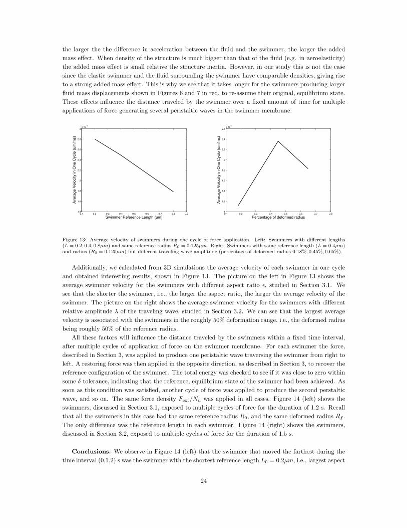
the larger the the di↵erence in acceleration between the fluid and the swimmer, the larger the added

mass e↵ect. When density of the structure is much bigger than that of the fluid (e.g. in aeroelasticity)

the added mass e↵ect is small relative the structure inertia. However, in our study this is not the case

since the elastic swimmer and the fluid surrounding the swimmer have comparable densities, giving rise

to a strong added mass e↵ect. This is why we see that it takes longer for the swimmers producing larger

fluid mass displacements shown in Figures 6 and 7 in red, to re-assume their original, equilibrium state.

These e↵ects influence the distance traveled by the swimmer over a fixed amount of time for multiple

applications of force generating several peristaltic waves in the swimmer membrane.

0.1 0.2 0.3 0.4 0.5 0.6 0.7 0.8 0.91.4

1.6

1.8

2

2.2

2.4

2.6

2.8

3x 10

−3

Swimmer Reference Length (um)

Ave

rag

e V

elo

city

in O

ne

Cyc

le (

um

/ms)

0.1 0.2 0.3 0.4 0.5 0.6 0.7 0.81

1.2

1.4

1.6

1.8

2

2.2

2.4

2.6x 10

−3

Percentage of deformed radiusA

vera

ge

Ve

loci

ty in

On

e C

ycle

(u

m/m

s)

Figure 13: Average velocity of swimmers during one cycle of force application. Left: Swimmers with di↵erent lengths(L = 0.2, 0.4, 0.8µm) and same reference radius R0 = 0.125µm. Right: Swimmers with same reference length (L = 0.4µm)and radius (R0 = 0.125µm) but di↵erent traveling wave amplitude (percentage of deformed radius 0.18%, 0.45%, 0.65%).

Additionally, we calculated from 3D simulations the average velocity of each swimmer in one cycle

and obtained interesting results, shown in Figure 13. The picture on the left in Figure 13 shows the

average swimmer velocity for the swimmers with di↵erent aspect ratio , studied in Section 3.1. We

see that the shorter the swimmer, i.e., the larger the aspect ratio, the larger the average velocity of the

swimmer. The picture on the right shows the average swimmer velocity for the swimmers with di↵erent

relative amplitude of the traveling wave, studied in Section 3.2. We can see that the largest average

velocity is associated with the swimmers in the roughly 50% deformation range, i.e., the deformed radius

being roughly 50% of the reference radius.

All these factors will influence the distance traveled by the swimmers within a fixed time interval,

after multiple cycles of application of force on the swimmer membrane. For each swimmer the force,

described in Section 3, was applied to produce one peristaltic wave traversing the swimmer from right to

left. A restoring force was then applied in the opposite direction, as described in Section 3, to recover the

reference configuration of the swimmer. The total energy was checked to see if it was close to zero within

some tolerance, indicating that the reference, equilibrium state of the swimmer had been achieved. As

soon as this condition was satisfied, another cycle of force was applied to produce the second perstaltic

wave, and so on. The same force density Fext

/Nn

was applied in all cases. Figure 14 (left) shows the

swimmers, discussed in Section 3.1, exposed to multiple cycles of force for the duration of 1.2 s. Recall

that all the swimmers in this case had the same reference radius R0

, and the same deformed radius Rf

.

The only di↵erence was the reference length in each swimmer. Figure 14 (right) shows the swimmers,

discussed in Section 3.2, exposed to multiple cycles of force for the duration of 1.5 s.

Conclusions. We observe in Figure 14 (left) that the swimmer that moved the farthest during the

time interval (0,1.2) s was the swimmer with the shortest reference length L0

= 0.2µm, i.e., largest aspect

24

0 200 400 600 800 1000 1200 1400 16000.5

0.55

0.6

0.65

0.7

0.75

0.8

0.85

0.9

0.95

1

T (ms)

His

tory

of th

e s

wim

mer

cente

r (µ

m)

L0 = 0.2 µm

L0 = 0.4 µm

L0 = 0.8 µm

0 200 400 600 800 1000 1200 1400 16000.5

0.55

0.6

0.65

0.7

0.75

0.8

0.85

0.9

0.95

1

T (ms)

His

tory

of th

e s

wim

mer

cente

r (µ

m)

Rf = 0.82R

s

Rf = 0.55R

s

Rf = 0.35R

s

Figure 14: The figures show history of swimmers center for multiple cycles of force application. Left: comparison betweenswimmers of di↵erent reference length, same reference radius R0 = 0.125µm, and same deformed radius Rf = 0.55R0, c.f.Figure 6. Right: comparison between swimmers with di↵erent deformed radius, same reference radius R0 = 0.125µm andsame reference length L = 0.4µm, c.f. Figure 8.

ratio = R0

/L. Even though the displaced mass during one cycle was the smallest for this swimmer,

the rate of displaced mass per second is the largest, as shown in Figure 13 (left). This, combined with

the smallest added mass e↵ect associated with this swimmer, produces the fastest swimmer overall when

swimmers with di↵erent aspect ratio are considered.

Figure 14 (right) shows, on the other hand, that all three swimmers produce roughly the same distance

traveled during the time interval (0, 1.5)s. One can notice that the average slope corresponding to the

black curve is slightly bigger, indicating that for longer distances the motion of the swimmer with the

deformed swimmer radius of roughly 50% of the reference radius, is the “optimal” solution. This is

consistent with the result shown in Figure 13 (right), which indicates that swimmers with roughly 50%

of deformation have the largest average velocity in one cycle of force application.

Thus, our study indicates that fast swimmers are those with large aspect ratios whose radius deforms

roughly 50% in each cycle. Such swimmers are capable of generating a large number of contractions per

unit time because of their short length, producing the largest rate of change of displaced mass per unit

time.

5. Conclusions

We conclude this manuscript by showing in Figure 15 three “representative” snap shots of the motion

of our “optimal swimmer” with R0

= 0.125, L = 0.2 and Rf

= 0.55R0

over multiple (10) cycles,

corresponding to the blue curve in Figure 14 (left). We calculated the distance traveled by the swimmer

and obtained that within one second our “optimal swimmer” traversed the distance equal to 1.5 of the

swimmer lengths. Figure 16 shows the first and last snap shot superimposed, indicating the traversed

distance.

The results of our work are consistent with the results reported in the review article [11] published

in 2014 in Micromachines. In fact, our swimmers are at the top of the class of all artificial swimmers

swimming at low Reynolds numbers reported in [11]. More precisely, the authors of [11] obtained

a diagram comparing propulsion speed versus Reynolds numbers for 18 artificial (manufactured) and

natural micro swimmers. It was concluded that artificial micro-swimmers in general travel slower than

the natural ones, and that at low Reynolds numbers the speed of artificial micro-swimmers is between

0.6 and 2 body length per second at the Reynolds numbers around 106. Therefore, the results of our

research are very relevant, and are a first step in our long-term goal to design a medical micro-swimmer

25

Figure 15: Motion of the swimmer with R0 = 0.125, L = 0.2 and Rf = 0.55R0 over multiple (10) cycles, corresponding tothe blue curve in Figure 14 (left). Three “representative” snap shots are shown at t = 1ms, t = 507ms, and t = 1000ms.

based on the contractions of a cylindrical membrane lined with cardiac myocytes capable of producing

coordinated contractions [15].

Figure 16: Two snap shots from Figure 15 (first and last) superimposed. The figure indicates that the swimmer hastraversed the distance equal to 1.5 reference lengths.

Acknowledgments

The authors would like to thank Dr. Richard D. James for bringing this problem to their attention

while meeting at Oxford University in 2014. The research in this work has been partially supported

by the National Science Foundation under grants NSF DMS-1262385 (Canic, Quaini, Shi), NSF DMS-

1311709 (Canic), NSF DMS-1318763 (Canic), and NSF/NIGMS DMS-1263572 (Canic, Quaini, Shi),

NSF DMS-1418308 (Pan).

References

[1] J. Adams, P. Swarztrauber, and R. Sweet, FISHPAK: A package of Fortran subprograms for the

solution of separable elliptic partial di↵erential equations, The National Center for Atmospheric

Research, Boulder, CO, 1980.

[2] A. Adjari, and H. A. Stone, A note on swimming using internally generated traveling waves,

Physics of Fluids, 11(5), 1999, 1275–1277.

[3] W. Alt, and M. Dembo, Cytoplasm dynamics and cell motion: twophase flow models, Mathemat-

ical Biosciences, 156, 1999, 207–228.

26

[4] V. Aranda, R. Cortez and L. Fauci. A model of Stokesian peristalsis and vesicle transport in a

three-dimensional closed cavity. J. Biomechanics, Vol. 48 (9), (2015) 1631-8.

[5] C.J. Brokaw, Simulating the e↵ects of fluid viscosity on the behavior of sperm flagella, Mathe-

matical Methods in the Applied Sciences, 24, 2001, 1351–1365.

[6] S. Canic, E-H. Kim. Mathematical Analysis of the Quasilinear E↵ects in a Hyperbolic Model of

Blood Flow through Compliant Axisymmetric Vessels, Mathematical Methods in Applied Sciences,

26 (14), 2003, 1161–1186.

[7] E.J. Dean, and R. Glowinski, A wave equation approach to the numerical solution of the Navier–

Stokes equations for incompressible viscous flow, C.R. Acad. Sc. Paris, Serie 1, 325, 1997, 783–

791.

[8] E.J. Dean, R. Glowinski, and T.W. Pan, A wave equation approach to the numerical simulation

of incompressible viscous fluid flow modeled by the Navier–Stokes equations, In Mathematical and

Numerical Aspects of Wave Propagation, De Santo JA (Ed.), SIAM: Philadelphia, 1998, 65–74.

[9] R. Dreyfus, J. Baudry, M.L. Roper, M. Fermigier, H.A. Stone, and J. Bibette, Microscopic artificial

swimmers, Nature, 437, 2005, 862–865.

[10] T. Ebefors, and G. Stemme, The MEMS handbook, Chapter 28- Micro-robotics, CRC Press, 2002,

28-1 – 28–42.

[11] J. Feng, and S. K. Cho, Mini and Micro Propulsion for Medical Swimmers (Review), Microma-

chines 5, 2014, 97–113.

[12] R. Glowinski, Finite element methods for incompressible viscous flow, In Handbook of Numerical

Analysis, Vol. IX, Ciarlet PG and Lions JL (Eds.), North–Holland: Amsterdam, 2003, 7–1176.

[13] S. Guo, Y. Okuda, and K. Asaka, Hybrid type of underwater microbiped robot with walking and

swimming motions, IEEE Conference on Robotics and Automation (ICRA’05), 3, 2004, 1604–

1609.

[14] C. Hamlet, L. Fauci and E.D. Tytell. The e↵ect of intrinsic muscular nonlinearities on the en-

ergetics of locomotion in a computational model of an anguilliform swimmer. J. Theor. Biol. To

appear (2015).

[15] L. Khait, and R.K. Birla, Cell-based cardiac pumps and tissue-engineered ventricles, Regenerative

Medicine 2(4), 2007, 391–406

[16] G. Kosa, M. Shoham, and M. Zaaroor, Propulsion Method for Swimming Micro Robots, IEEE

Transaction on Robotics, 23, 2007, 137–150.

[17] G. Kosa, and Peter Jakab, Nobuhiko Hata, Ferenc Jolesz, Zipi Neubach, Moshe Shoham, Menashe

Zaaroor, and Gabor Szekely, Flagellar swimming for medical micro robots: Theory, experiments

and application, Biomedical Robotics and Biomechatronics, 2008. BioRob 2008. 2nd IEEE RAS

& EMBS International Conference 2008, 258 – 263.

[18] M.A. Mohamed, M.K. Hogan, N.M. Patel, Z-w. Tao, L. Gutierrez, and R.K. Birla, Establishing

the Framework for Tissue Engineered Heart Pumps, Cardiovacular Engineering and Technology,

Published online January 2015.

[19] Y. Okada, S. Takeda, Y. Tanaka, J.C. Belmonte, and N. Hirokawa, Mechanism of Nodal Flow: A

Conserved Symmetry Breaking Event in Left-Right Axis Determination, Cell, 121, 2005, 633–644.

27

[20] T.W. Pan, and R. Glowinski, Direct simulation of the motion of neutrally buoyant balls in a

three–dimensional Poiseuille flow, C. R. Mecanique, 333, 2005, 884–895.

[21] C.S. Peskin, Numerical analysis of blood flow in the heart, J. Comput. Phys., 25, 1977, 220–252.

[22] C.S. Peskin, and McQueen D.M., Modeling prosthetic heart valves for numerical analysis of blood

flow in the heart, J. Comput. Phys., 37, 1980, 11332.

[23] C.S. Peskin, The immersed boundary method, Acta Numer., 11, 2002, 479–517.

[24] J. Simons, L. Fauci and R. Cortez. A fully three-dimensional model of the interaction of driven

elastic filaments in a Stokes flow with applications to sperm motility. J. Biomechanics, 48 (9),

2015, 1639-1651.

[25] L. Shi, T.W. Pan, and R. Glowinski, Three-dimensional simulation of red blood cell motion in

Poiseuille flows, International Journal for Numerical Methods in Fluids, 76, 2014, 397–415.

[26] D. Takagi, and N. J. Balmforth, Peristaltic pumping of rigid objects in an elastic tube, J. Fluid

Mech., 672, 2011, 219–244.

[27] M. Tanaka, S. Wada and M. Nakamura. Computational Biomechanics: Theoretical Background

and Biological/Biomedical Problems. Springer, 2012 ISBN-13: 978-4431540724.

[28] E. Tytell, C. Hsu, T. Williams, A. Cohen and L. Fauci. Interactions between internal forces, body

sti↵ness, and fluid environment in a neuromechanical model of lamprey swimming. Proc. National

Acad. of Sciences 107, 2010, 19832-19837.

[29] S. Wada, and R. Kobayashi, Numerical simulation of various shape changes of a swollen red blood

cell by decrease of its volume, Trans. JSME. Ser. A, 69, 2003, 14–21.

[30] T.Y.T. Wu, C.J. Brokaw, and C. Bremmen Edt, Swimming and flying in nature, New York:

Plenum Press, 1975, pp.161-173.

[31] K.B. Yesin, K. Vollmers, and B.J. Nelson, Modeling and control of untethered biomicrorobots

in a fluidic environment using electromagnetic fields, International Journal of Robotics Research,

25, 2006, 527–536.

28