a step-up multiple test procedure - northwestern...

A Step-Up Multiple Test ProcedureAuthor(s): Charles W. Dunnett and Ajit C. TamhaneSource: Journal of the American Statistical Association, Vol. 87, No. 417 (Mar., 1992), pp. 162-170Published by: American Statistical AssociationStable URL: http://www.jstor.org/stable/2290465Accessed: 21/10/2010 17:48

Your use of the JSTOR archive indicates your acceptance of JSTOR's Terms and Conditions of Use, available athttp://www.jstor.org/page/info/about/policies/terms.jsp. JSTOR's Terms and Conditions of Use provides, in part, that unlessyou have obtained prior permission, you may not download an entire issue of a journal or multiple copies of articles, and youmay use content in the JSTOR archive only for your personal, non-commercial use.

Please contact the publisher regarding any further use of this work. Publisher contact information may be obtained athttp://www.jstor.org/action/showPublisher?publisherCode=astata.

Each copy of any part of a JSTOR transmission must contain the same copyright notice that appears on the screen or printedpage of such transmission.

JSTOR is a not-for-profit service that helps scholars, researchers, and students discover, use, and build upon a wide range ofcontent in a trusted digital archive. We use information technology and tools to increase productivity and facilitate new formsof scholarship. For more information about JSTOR, please contact [email protected].

American Statistical Association is collaborating with JSTOR to digitize, preserve and extend access to Journalof the American Statistical Association.

http://www.jstor.org

http://www.jstor.org/action/showPublisher?publisherCode=astata

http://www.jstor.org/stable/2290465?origin=JSTOR-pdf

http://www.jstor.org/page/info/about/policies/terms.jsp

http://www.jstor.org/action/showPublisher?publisherCode=astata

A Step-Up Multiple Test Procedure CHARLES W. DUNNETT and AJIT C. TAMHANE*

We consider the problem of simultaneously testing k 2 2 hypotheses on parameters 01 . ok. In a typical application the O's may be a set of contrasts, for instance, a set of orthogonal contrasts among population means or a set of differences between k treatment means and a standard treatment mean. It is assumed that least squares estimators 01, ..., ok are available that are jointly normally distributed with a common variance (known up to a scalar, namely the error variance ao2) and a common known correlation. An independent x2-distributed unbiased estimator of a-2 is also assumed to be available. We propose a step-up multiple test procedure for this problem which tests the t statistics for the k hypotheses in order starting with the least significant one and continues as long as an acceptance occurs. (By contrast, the step-down approach, which is usually used, starts with the most significant and continues as long as a rejection occurs.) Critical constants required by this step-up procedure to control the type I familywise error rate at or below a specified level a are computed for both one-sided and two-sided testing problems. Power comparisons are made for one-sided testing problems with the well-known normal theory based single-step and step-down test procedures, and also with a step-up test procedure proposed for a wider class of problems by Hochberg. (Two improvements over Hochberg's procedure by Hommel and Rom provide at best marginal increases in power, with the former being also more difficult to apply, and hence they are not included here.) Two different definitions of power are considered-the probability of rejecting all false hypotheses and the probability of rejecting at least one false hypothesis; the results are found to be qualitatively similar. The proposed step-up procedure is more powerful than the single-step procedure except when only one hypothesis is false, in which case it is slightly less powerful. Similarly, it is slightly less powerful than the step-down procedure when a few hypotheses are false, but it is more powerful when most or all hypotheses are false, and this power advantage increases with the number of such hypotheses under test. The proposed step-up procedure is uniformly more powerful than the Hochberg procedure and its improvements. A disadvantage of the proposed step-up procedure is the greater difficulty of computing its critical points. These are given for one-sided and two-sided tests for 5% level of significance.

KEY WORDS: Comparisonwise approach; Experimentwise approach; Familywise error rate; Joint p-values; Multiple comparison procedures; Multivariate t distribution; Power; Single-step procedure; Step-down procedure.

1. INTRODUCTION

The purpose of many empirical studies is to compare several treatment groups by estimating differences or by per- forming tests of significance on relevant parameters. Such multiple comparisons in the same study are the rule rather than the exception. There has been much debate and con- troversy as to whether statistical adjustments are necessary for taking into account the multiplicity of inferences. One school of thought, as advanced by Miller (1966), Scheff6 (1953), Tukey (1953), and others, is that such adjustments should be made by requiring the inference procedures to satisfy the condition that the probability of at least one wrong inference (e.g., at least one type I error in a multiple hypothesis testing problem) is controlled at or below a specified level a. This is called the "experimentwise" or the "familywise" error rate (FWE) control approach. The op- posite school of thought, as represented, for example, by Carmer and Walker (1982), Nelder and some other discus- sants of O'Neill and Wetherill (1971), O'Brien (1983), Perry (1986), and Rothman (1990), maintains that such adjustments are not needed and that each inference should be dealt with separately, which is referred to as the "comparisonwise" error rate control approach. A third school of thought, led by Duncan [e.g., Duncan (1965), Waller and Duncan

* Charles W. Dunnett is Professor Emeritus, Department of Mathe- matics and Statistics and the Department of Clinical Epidemiology and Biostatistics, McMaster University, Hamilton, Ontario, Canada L8S 4K1. Ajit C. Tamhane is Professor, Department of Statistics and the Depart- ment of Industrial Engineering and Management Sciences, Northwestern University, Evanston, IL 60208. Charles W. Dunnett's research was sup- ported by the Natural Sciences and Engineering Research Council of Can- ada. The authors thank Anthony J. Hayter for his help in investigating the existence of critical constants for the proposed procedure. The authors are also grateful to the two referees for their suggestions, which greatly improved the article.

(1969), Duncan and Dixon (1983)] adopts a Bayesian decision-theoretic approach to multiple comparisons problems assuming prior distributions on the unknown parameters, linear loss functions for type I and type II errors for indi- vidual significance tests, and an additive loss function for the overall loss. For the pairwise comparison problem, the resulting test procedure has the nature of a comparisonwise procedure in the sense that the critical constant it uses does not depend on the number of comparisons (as do the critical constants used by the familywise procedures); however, it does differ from the customary comparisonwise procedures [e.g., the unprotected least significant difference (LSD) test] by making this constant depend in an inverse way on the analysis of variance F statistic, which is a sample measure of the disparity between the treatment means being compared.

The use of the experimentwise approach is called for in the following situations: (1) when a conclusion is reached that requires the simultaneous correctness of several inferences and (2) when a conclusion is reached that hinges on the correctness of an inference that has been selected in light of the data. For example, consider a pharmaceutical company that compares several drugs with a standard in the same study for the purpose of determining which ones give the most improvement, with the goal of selecting one of them to recommend for further developmental work. If the drug that happens to be selected for this purpose is, in fact, inferior to the standard, then a serious error would be made. Therefore, it is necessary to control the probability of making such an error, which is achieved by using the experimentwise approach. On the other hand, if several treatments are included in the same experiment solely for the

? 1992 American Statistical Association Joumal of the American Statistical Association

March 1992, Vol. 87, No. 417, Theory and Methods

162

Dunnett and Tamhane: A Step-Up Multiple Test Procedure 163

purpose of economy and efficiency, and the comparisons of interest are inherently separate from each other and could logically have been examined in separate experiments were it not for the inefficiency of doing this, then the comparisonwise approach is appropriate (O'Brien 1983). Duncan's approach offers an alternative solution to multiple comparisons if the underlying assumptions, particularly the one concerning the additive form of the overall loss function (which is the reason for the comparisonwise nature of the procedure), are satisfied.

A criticism of the experimentwise approach sometimes made is that it lowers the power of detecting real effects due to the stricter requirement on the type I error rate. One way of increasing power, when inferences are in the form of hypotheses tests, is to employ stepwise tests. The purpose of this article is to develop a new stepwise procedure of the step-up type for testing multiple hypotheses under the framework of the experimentwise approach and compare its performance with a step-down procedure. We consider the problem of simultaneously testing k ' 2 hypotheses, H1, H2, ..., Hk, subject to the requirement that the type I FWE, which is the probability of rejecting any true hypothesis, be kept at or below a specified level a (referred to as the overall significance level). All procedures considered in this article satisfy this requirement. Some assume specific parametric distributional models, while others are more general. The prime example in this latter class is the well-known Bonferroni procedure, which rejects any Hi with pi ' a/k, where pi is the p value computed from the observed value ti of some test statistic Ti for Hi (1 ' i ' k). For large k, the Bonferroni procedure becomes increasingly conservative, and hence modifications of it with improved powers have been proposed. One procedure due to Holm (1979) proceeds as follows: Order the p values, P(1) 2 >** p(k), and denote the corresponding hypotheses, H(l),

H(k). Start with the smallest p value, P(k). If p(k) > a/k, then stop testing and accept all the hypotheses; otherwise reject H(k) and go to the next step. In general, if testing has continued to the ith step (1 ' i ' k) and if P(k-i+l) > a/ (k - i + 1), then stop testing and accept all the remaining hypotheses, H(k1i+l), . . ., H(1); otherwise reject H(k.i+l) and go to the next step. Another procedure due to Hochberg (1988) proceeds as follows: Start with the largest p value, P(1). If P(1) ' a then stop testing and reject all the hypotheses; otherwise accept H(I) and go to the next step. In general, if testing has continued to the ith step (1 ' i ' k) and if P(i) 'c a/i, then reject all the remaining hypotheses, H(i), . . ., H(k); otherwise accept H(i) and go to the next step. It is readily seen that the Holm procedure is uniformly less powerful than the Hochberg procedure, since the latter al- ways rejects any hypothesis rejected by the former. This results from the fact that both use the same critical values for the P(i), but the Holm procedure uses a step-down algorithm, while the Hochberg procedure uses a step-up algorithm for making accept or reject decisions. Also note that the Holm procedure, in turn, is uniformly more powerful than the Bonferroni procedure, which is said to be of the single-step type (Hochberg and Tamhane 1987, chap. 2).

In the parametric case, normal theory based single-step and step-down procedures have been developed (described in Section 2.2), but hardly any attention has been paid to the step-up approach (the only exception to our knowledge being one proposed by Welsch (1977) for the pairwise comparisons problem). In this article, we introduce a new step- up procedure for the problem of testing a nonhierarchical family of hypotheses (Hochberg and Tamhane 1987, chap. 2) on k > 2 linear parametric functions (e.g., contrasts) and compare its performance with a competing step-down procedure. The development is restricted to balanced data situations, but extensions to unbalanced cases are covered briefly in Section 8.

2. PRELIMINARIES

2.1 Distributional Setup

We assume the standard normal theory linear model setting. Thus consider k ? 2 parameters 01, ., ok, and let

A A

their unbiased least squares estimators 01, . . k be jointly normally distributed with var (0i) = O2T2 and corr (0i, Oj) = p, where r2 and p are known constants depending on the design and OC2 iS the unknown error variance. Let S2 be an unbiased estimator of OC2 having v df such that vS2/r-2 has a x2 distribution independent of the Oi. Finally, let 0 denote the vector (01, ..., Ok)-

Typically the Oi are contrasts among some population means. Three examples of this setting are: (1) orthogonal contrasts in a balanced design for which we have T2 =I ci2, where the cij are the contrast coefficients for the ith contrast Oi (1 ' i ' k) and p = 0; (2) comparisons of k treatment means with a control mean in a one-way layout with no observations on the control and n observations on each treatment, which leads to T2 = l/no + 1/n and p = nl(no + n); and (3) comparisons of k treatment means with a control mean in a balanced treatments incomplete block (BTIB) design, where the formulas for r2 and p are given by (4.3) and (4.4), respectively, of Bechhofer and Tam- hane (1981).

2.2 Hypotheses and Test Procedures Consider k ? 2 upper one-sided hypothesis testing prob-

lems, Hi : Oi = 0 versus Ki : Oi > 0 (1 ? i ' k). Suppose that the type I FWE is to be controlled at a specified level a. In other words, if Om is any parameter configuration 0 with Oi = O, fori = 1, ...,mand Oi > fori = m + 1, ... k, then we require

Pom{Accept H1, . . ., Hm} 1 - a,

m1= ,...,k. (2.1)

Let ti = oi/sT (where s is the observed value of S) be the usual t statistic for testing Hi (1 ' i ? k). If H1, * .., H, are true, then the corresponding random variables T1, Tm have Student's m-variate central t distribution with v df and associated common correlation coefficient p (m = 1,

k). Let cm = t ()p be the upper a point of maxl5i,m T1, for m = 1, ..., k. Bechhofer and Dunnett (1988) have given extensive tables of cm' values. For m =1, we have cl= 4(v, the upper az point of Student's univariate t dis-

tribution with vi df.

164 Journal of the American Statistical Association

The usual single-step test procedure (SS) rejects any Hi with ti ' c', for example, Dunnett's (1955) procedure for the comparisons with a control problem. For the same problem, the usual step-down test procedure (SD), as proposed originally by Miller (1966, pp. 78 and 85-86) and later studied by Naik (1975) and Marcus, Peritz, and Gabriel (1976), first orders the statistics as t(1) s*- c t(k) (and the corresponding hypotheses as H(l), ..., H(k)), and then rejects any H(i) iff H(j) is rejected for j = k, . . ., i + 1 and t(i) >' c'. Both of these procedures control the type I FWE at level a; see Hochberg and Tamhane (1987, chap. 2, Secs. 2.1.1 and 4.2). Since c,' < c' for i < k, it is clear that SD is uniformly more powerful than SS.

Our proposed step-up procedure (SU) will be based on another set of critical constants cl ? c2 ? ... ? ck (to be defined shortly). It will accept H(i) iff H(j) is accepted for j = 1, ..., i-l and t(i) < ci. Thus SU will begin by testing the smallest t statistic and work upward, accepting one hypothesis at a time and stopping by rejecting H(), H(i+1)9 .... H(k) when t(i) ? ci.

3. DETERMINATION OF CRITICAL CONSTANTS

3.1 Maximum Type I Familywise Error Rate

The critical constants of the SU procedure are to be determined so that the type I FWE requirement (2.1) is satisfied. Therefore, we first need to determine the maximum type I FWE or, equivalently, the minimum of the left side of (2.1), the minimum being taken over all Hm, for each m - 1, ..., k. This is done in the following theorem.

Theorem 3.1. Suppose that H1, ..., Hm are true and that Hm+i, . . ., Hk are false (m = 1, ..., k). Then, for the SU procedure, the left side of (2.1) is minimized over Om when Oi -> oo, for i = m + 1, ..., k.

The proof of this theorem is given in Dunnett and Tam- hane (1990) (hereafter abbreviated as DT), and is similar to the first part of the proof of Theorem 1 in Hayter and Tamhane (1990). In fact, using ideas similar to those in the second part of that proof, we can show that the left side of (2.1) is minimized over Oi < 0, for i = 1, ..., m, when they are all equal to zero. In other words, we can consider the hypotheses Hi: Oi < 0 (1 i ? k) instead of Hi: O - 0 (1 ? i ? k) as considered here for convenience.

3.2 Properties of Critical Constants

To satisfy (2.1), the critical constants of the SU procedure must be determined so that the minimum found in Theorem 3.1 is at least 1 - a for each m = 1, 2, .... The smallest possible value for each cm is found by solving the following equation, obtained by setting this minimum equal to 1 - a:

PJ(T19 *--,Tm) < (C1, ..., cm1)} = 1 -Ca; (3.1)

here T1, ..., Tm are as defined in Section 2.2, and (xl,... Xm) < (Yi,. .,Ym) denotes that Xism < Yi,m X2,m < Y2,m,*

Xm,m K Ym,m where the Xi,m and Yi are the ordered xi and yi.

Although we have not been able to show analytically that solutions cl, c2, ..., cm satisfying the monotonicity condition cl ' C2 ' .. c? m < Xo exist for arbitrary m, we have been able to show this for m = 2; see DT. Moreover, our computational experience for m ' 8 and a = .05 indicates that they probably exist for the values of m likely to be encountered in practice. (In the case of independent test statistics, we have verified this for m as large as 1,000.) Finner, Roters, and Hayter (1991) have recently addressed this problem.

We next compare the critical constants used by the SU, SD, and Hochberg's (1988) step-up procedure (henceforth referred to as the HC procedure).

Proposition 3.]. Let cm, c', and cm = t (/m) (m = 1, 2, ...) denote the critical constants used by the SU, SD, and HC procedures, respectively. We have

cl = c ' = tc(a) and Cm < Cm < C, m > 1. (3.2)

Proof. The first part of (3.2) is obvious. The inequality cm < cm for m > 1 follows by comparing Equation (3.1) for cm with the following equation for c':

P{Tm,m < c } = 1 -a, m = 1, ..., k,

where Tm,m = max(TI, ..., Tm). We have proved the inequality cm < cm only for m = 2

in DT, and we conjecture it to be true for m > 2.

Since the critical constants used by SU are larger than those used by SD, except for m = 1, when they are equal, we cannot say that SU will be uniformly more powerful than SD, as was the case between Hochberg's step-up procedure and Holm's step-down procedure. SU will, however, be uniformly more powerful than HC because of the inequality cm < cm for m > 2. This is, of course, not sur- prising since HC does not exploit the correlation structure between the test statistics as does SU.

As noted before, the critical constants c,' are extensively tabulated by Bechhofer and Dunnett (1988). The critical constants cm, being the percentiles of the univariate Stu- dent's t distribution, can also be readily obtained. Exact computations show that cm is much closer to c' than to cm; see Table 5.

3.3 Computation of Critical Constants

From (3.1) we see that the critical constants must be computed recursively; to determine cm, one must first know the values of cl, ..., cm-,. This is in contrast to the computation of the critical constants c' = t-

( for the SD procedure which, for different values of m, can be computed independently of each other. To compute cm, for m > 1, we now derive a general expression for the left side of (3.1) that can be evaluated efficiently on a computer.

Let Zi, for i = 0, 1, . . ., k, be independent N(O, 1) random variables, and let U be a y/v random variable independent of the Z,. Then we can express Ti -

{A/1 - pZ, - \/7Z0}/U (1 ? i ? m) and write the desired probability as


f P{(Z1 .* . . zm)

< (dig ... * dm)}4(zo) dzofv(u) du, (3.3) where di = (ciu + \/pzO)/\/I7p (1 ' i ' in), m fq(zo) is the standard normal density function, and f,(u) is the density function of U. A recursive formula for the probability term in the integrand of (3.3) is obtained in the following lemma.

Lemma 3.1. Let '(1 ) denote the standard normal distribution function. We have

P{(V1 9 . .. 9 Zm) < (di, d * * * dm)}

= P{(Z1, i.., Zm_1) < (d2, ..., dm)}ti(di)

+ P{(Z1, ., Z m_) < (dl, d3, ..., dm)}{4>(d2) - (di)}

+ P{(Z1, ..., Zm_1) < (di, ..., dm_i)}{4>(dm) - 'I(dm,)}.

(3.4)

Proof. The result follows by successively conditioning Zm to lie in the intervals (-oo, d1), [dl, d2), ..., [dmili dm). Note that we do not condition Zm to lie in the interval [dm, oo) because, in that case, the event {(Z1, ... , Zm) < (d, * * I dm)} is not satisfied.

Let (12 m denote the expression in (3.4). An algorithm for computing (12 m is as follows.

Step 1. Calculate (h = 'F(dh), for h = 1, ..., m, a total of m terms.

Step 2. Calculate 'Dhi = (i)h + I'h['I'i - (h], for 1 I h < i ? mi, a total of (m) terms.

Step 3. Calculate 'Dhij = sijsh + -hj[?i h] + (hi[?j - D)i], for 1 ' h < i < j _ mi, a total of (m) terms.

Step m. Calculate 412 m = 4>'2 m4>'1 + (P13 m[(P2 - (DI] + + (Pi.* m-I [(DMm 4 \m-1] -

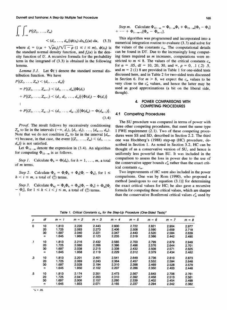
This algorithm was programmed and incorporated into a numerical integration routine to evaluate (3.3) and solve for the values of the constants cm. The computational details can be found in DT. Due to the increasingly long computing times required as m increases, computations were restricted to m ' 8. The values of the critical constants cm for a = .05, df = 10, 20, 30, and oo, p = 0, .1 (.2) .5, and m = 2 (1) 8 are provided in Table 1 for one-sided tests discussed here, and in Table 2 for two-sided tests discussed in Section 6. For m > 8, we expect the cm values to be very close to the cm values, and hence the latter may be used as good approximations (a bit on the liberal side, though).

4. POWER COMPARISONS WITH COMPETING PROCEDURES

4.1 Competing Procedures

The SU procedure was compared in terms of power with three other competing procedures, that meet the same type I FWE requirement (2.1). Two of these competing procedures were SS and SD, described in Section 2.2. The third one was Hochberg's (1988) step-up (HC) procedure, described in Section 1. As noted in Section 3.2, HC can be thought of as a conservative version of SU, and hence is uniformly less powerful than SU. It was included in the comparison to assess the loss in power due to the use of the conservative upper bounds cm rather than the exact critical constants cm.

Two improvements of HC were also included in the power comparisons. One was by Rom (1990), who proposed a method [analogous to our equation (3.1)] for determining the exact critical values for HC; he also gave a recursive formula for computing these critical values, which are sharper than the conservative Bonferroni critical values cm used by

Table 1. Critical Constants Cm for the Step-Up Procedure (One-Sided Tests)*

p df m= 1 m= 2 m= 3 m = 4 m= 5 m= 6 m= 7 m= 8

0 10 1.813 2.220 2.44$ 2.600 2.722 2.821 2.904 2.977 20 1.725 2.083 2.273 2.406 2.508 2.590 2.659 2.718 30 1.697 2.040 2.221 2.347 2.443 2.520 2.584 2.639 00 1.645 1.960 2.123 2.235 2.319 2.386 2.442 2.490

.1 10 1.813 2.216 2.432 2.585 2.703 2.799 2.879 2.949 20 1.725 2.080 2.266 2.396 2.496 2.576 2.644 2.701 30 1.697 2.038 2.215 2.338 2.432 2.508 2.571 2.625 00 1.645 1.958 2.119 2.229 2.312 2.379 2.434 2.482

.3 10 1.813 2.201 2.401 2.541 2.649 2.736 2.810 2.873 20 1.725 2.069 2.243 2.364 2.457 2.532 2.594 2.648 30 1.697 2.028 2.194 2.310 2.398 2.469 2.528 2.579 00 1.645 1.950 2.102 2.207 2.286 2.350 2.403 2.448

.5 10 1.813 2.174 2.351 2.473 2.567 2.643 2.706 2.761 20 1.725 2.047 2.203 2.310 2.392 2.458 2.513 2.561 30 1.697 2.008 2.157 2.260 2.339 2.402 2.454 2.499 00 1.645 1.933 2.071 2.165 2.237 2.294 2.342 2.382

*a .05.


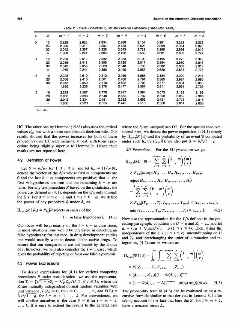
Table 2. Critical Constants Cm for the Step-Up Procedure (Two-Sided Tests)*

p df m= 1 m= 2 m= 3 m= 4 m= 5 m= 6 m= 7 m= 8

0 10 2.228 2.620 2.834 2.986 3.104 3.201 3.282 3.352 20 2.086 2.419 2.597 2.723 2.820 2.898 2.964 3.020 30 2.042 2.357 2.525 2.643 2.733 2.805 2.866 2.919 X0 1.960 2.241 2.389 2.492 2.569 2.631 2.683 2.727

.1 10 2.228 2.619 2.832 2.983 3.100 3.195 3.275 3.345 20 2.086 2.418 2.595 2.720 2.817 2.894 2.960 3.016 30 2.042 2.356 2.523 2.640 2.730 2.802 2.863 2.915 00 1.960 p.241 2.388 2.490 2.567 2.629 2.681 2.725

.3 10 2.228 2.610 2.812 2.955 3.065 3.154 3.229 3.294 20 2.086 2.410 2.581 2.700 2.791 2.865 2.927 2.980 30 2.042 2.350 2.510 2.622 2.708 2.777 2.834 2.883 00 1.960 2.236 2.378 2.477 2.551 2.611 2.661 2.703

.5 10 2.228 2.587 2.770 2.897 2.994 3.073 3.139 3.196 20 2.086 2.393 2.548 2.655 2.737 2.803 2.859 2.906 30 2.042 2.334 2.481 2.582 2.659 2.721 2.773 2.818 00 1.960 2.223 2.355 2.445 2.513 2.568 2.614 2.653

HC. The other one by Hommel (1988) also uses the critical values cm, but with a more complicated decision rule. Our results showed that the power increases for both of these procedures over HC were marginal at best, with Rom's procedure being slightly superior to Hommel's. Hence their results are not reported here.

4.2 Definition of Power

Let 8i = Oi/o-r for 1 ' i ' k, and let 8m = (I/orT)Om

denote the vector of the 8i's whose first m components are 0 and the last k - m components are positive; that is, the first m hypotheses are true and the remaining k - m are false. For any test procedure R based on the ti-statistics, the power, as defined in (4. 1), depends on the Oi's only through the 8i's. For 0 ' m ' k- land 1 ' t ' k-m, we define the power of any procedure R under 8m as

HIk,m,t(R I 8m) = PJm{R rejects at least t of the

k - m false hypotheses}. (4.1)

Our focus will be primarily on the t = k - m case since, in most situations, one would be interested in detecting all false hypotheses; for instance, in drug development studies one would usually want to detect all the active drugs. To ensure that our comparisons are not biased by the choice of t, however, we will also consider the t = 1 case, which gives the probability of rejecting at least one false hypothesis.

4.3 Power Expressions

To derive expressions for (4.1) for various competing procedures R under consideration, we use the representation T, = {I77pZ, - \?Z0}/U (1 ' i ' k), where the Zi are mutually independent normal random variables with unit variance, E(Zi) = 0, for i = 0, 1, . . ., m, and E(Zi) = 8 i/VTT7, for i = m + 1, ..., k. For convenience, we will confine ourselves to the case 8i 8 for i = m + 1, ... k. It is easy to extend the results to the general case

where the Si are unequal; see DT. For the special case considered here, we denote the power expression in (4. 1) simply by ['k,m,t(R I 5) and the probability of an event Z computed under such 8m by Ps,m(%); we also put A = //V 7.

SU Procedure. For the SU procedure we get k-m-t m\

llk,m,t(SU I 8) = I E k k-mr ( m

s=O r=O

x P8,m{accept H1, . . ., Hm+, . . Hm+s;

reject Hr?, . . ., Hm, Hm+s+i, * * H}

k-m-t m / k- (k-m ( ) s=O r=O

x P8,sm{(TI, 9 . Trg Tm+l I 9 9 TM+S) < (C,, *S Cr+s);

min (Tr+i, . . ., Tm, Tm+s+l, * *, Tk) ? Cr+s+l}. (4.2)

Now use the representation for the Ti's defined in the pre- ceding paragraph, condition on U = u and ZO = zo, and let di = (ciu + \/pzo)//1 - p (1 ' i ' k). Then, using the independence of the Zi's (1 ' i < k), unconditioning on U and ZO, and interchanging the order of summiation and integration, (4.2) can be written as

r?? r?? k-m-t m\ \

[Ik,m,t(SU I 8) = t r kfr=O (k - m m) JO -- s=0 r=0 \ r

x PIVZ1 . . Zr9 ZM+19 .. * Zm+s)

< (di, ... , dr+s)}[1 - 4>(dr+s+i)]m-r

X [1 _- (dr+s+i _- )]k-m-S (zo) dzof,(u) du. (4.3)

The probability term in (4.3) can be evaluated using a recursive formula similar to that derived in Lemma 3.1 after taking account of the fact that here the Zi, for i ? m + 1, have a nonzero mean A.


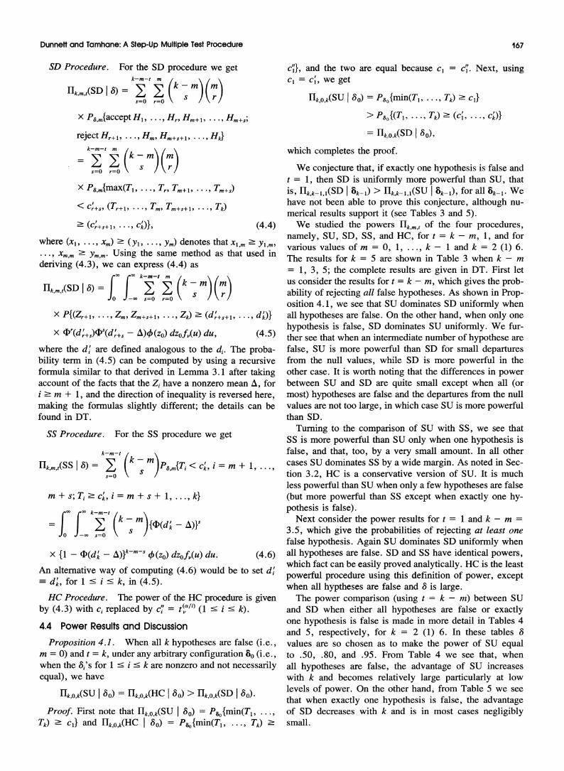
SD Procedure. For the SD procedure we get k-m-t m

rk,t(SD|8) = _ E k-m m s=O r=O\/

x P,,m{accept H1, . . ., Hr, Hm+, 1 . * ** Hm,s;

rejectHr+ 1, Hm, Hm+s+ ** Hkl k-m-tm

E Ek-m)(rn s=O r=O s

x P8,m{max(T19 ... 9 Trg Tm+lg . . TM+S)

<ICr+sg (Tr+19 . . Tmg Tm+s+l 1 . . TO)

(Cr+S+9 19** CkW9(44

where (xl, ..., pxm) 2 (Yl, . ., ym) denotes that xl,m ? Yl,rn ...X, xm 2 ym,m. Using the same method as that used in deriving (4.3), we can express (4.4) as

Hk,m,t(SD 1 8) = f j k - m) (m)

xPf(Zr+ 1 . .11 .m Z Zm+s+ 1 * .. * Zk) 2- (dr++' *9 * d)

X bT(d +s),Is(d +s- A)4(zo) dzof,(u) du, (4.5)

where the d' are defined analogous to the di. The probability term in (4.5) can be computed by using a recursive formula similar to that derived in Lemma 3.1 after taking account of the facts that the Zi have a nonzero mean A, for i 2 m + 1, and the direction of inequality is reversed here, making the formulas slightly different; the details can be found in DT.

SS Procedure. For the SS procedure we get

k-m-t

[Ik,m,t(SS I 8) = E k m)pmIT < Ck, i m + 1 * s=O

m +s; Ti 2 Ck'i = m +s+ 1,. ..., k}

rX 00 k-m-t

, _ A)k-ms {?(Z d k_ f}

X {1 - I(dk -)}kms 4 (Zo) dz0fv(U) du. (4.6)

An alternative way of computing (4.6) would be to set d' kd, for 1 s i s k, in (4.5).

HC Procedure. The power of the HC procedure is given by (4.3) with ci replaced by c' = t (cvi) (1 s i s k).

4.4 Power Results and Discussion

Proposition 4.1. When all k hypotheses are false (i.e., m = 0) and t = k, under any arbitrary configuration 80 (i.e., when the Si's for 1 s i s k are nonzero and not necessarily equal), we have

[Ik,O,k(SU | 80) = [Ik,ok(HC | 8o) > [Iko,k(SD | 80).

Proof. First note that [Ik,o,k(SU | 80) = P^0{min(T1, .. Tk) ? c1} and [Ik,ok(HC | 80) = P^0{min(T1, ..., Tk) ?

c%}, and the two are equal because cl = c7. Next, using cl = cl, we get

Hk,O,k(SU I ao) = P8J{min(T1, ..., Tk) 2 c1}

> P,6{(TI, . . ., Tk) 2 (c, ... * C)}

= Hk,o,k(SD I 80),

which completes the proof.

We conjecture that, if exactly one hypothesis is false and t = 1, then SD is uniformly more powerful than SU, that is, Hkk-1 1(SD I 8k-1) > Hk,k-,1 (SU I 8k-1), for all 8k-1 'We have not been able to prove this conjecture, although numerical results support it (see Tables 3 and 5).

We studied the powers ['k,m,t of the four procedures, namely, SU, SD, SS, and HC, for t = k - m, 1, and for various values of m = 0, 1, ..., k- 1 and k = 2 (1) 6. The results for k = 5 are shown in Table 3 when k - m = 1, 3, 5; the complete results are given in DT. First let us consider the results for t = k - m, which gives the probability of rejecting all false hypotheses. As shown in Prop- osition 4.1, we see that SU dominates SD uniformly when all hypotheses are false. On the other hand, when only one hypothesis is false, SD dominates SU uniformly. We further see that when an intermediate number of hypothese are false, SU is more powerful than SD for small departures from the null values, while SD is more powerful in the other case. It is worth noting that the differences in power between SU and SD are quite small except when all (or most) hypotheses are false and the departures from the null values are not too large, in which case SU is more powerful than SD.

Turning to the comparison of SU with SS, we see that SS is more powerful than SU only when one hypothesis is false, and that, too, by a very small amount. In all other cases SU dominates SS by a wide margin. As noted in Sec- tion 3.2, HC is a conservative version of SU. It is much less powerful than SU when only a few hypotheses are false (but more powerful than SS except when exactly one hypothesis is false).

Next consider the power results for t = 1 and k-m - 3.5, which give the probabilities of rejecting at least one false hypothesis. Again SU dominates SD uniformly when all hypotheses are false. SD and SS have identical powers, which fact can be easily proved analytically. HC is the least powerful procedure using this definition of power, except when all hyptheses are false and 8 is large.

The power comparison (using t = k - m) between SU and SD when either all hypotheses are false or exactly one hypothesis is false is made in more detail in Tables 4 and 5, respectively, for k = 2 (1) 6. In these tables 8 values are so chosen as to make the power of SU equal to .50, .80, and .95. From Table 4 we see that, when all hypotheses are false, the advantage of SU increases with k and becomes relatively large particularly at low levels of power. On the other hand, from Table 5 we see that when exactly one hypothesis is false, the advantage of SD decreases with k and is in most cases negligibly small.


Table 3. Probability of Rejecting At Least t of the k - m False Hypotheses [Power Ilk,m,t(R 86)] for Competing Procedures

Number of false Hi Procedure k- m t 8 SU SD SS HC

1 1 2 .408 .408 .408 .373 3 .777 .778 .778 .750 4 .961 .961 .961 .953

3 3 2 .228 .227 .173 .210 3 .649 .650 .578 .625 4 .933 .934 .906 .924

5 5 2 .293 .262 .106 .293 3 .736 .715 .477 .736 4 .963 .959 .866 .963

3 1 2 .659 .658 .658 .622 3 .941 .940 .940 .928 4 .997 .997 .997 .996

5 1 2 .775 .754 .754 .749 3 982 .971 .971 .979 4 1.000 .999 .999 1.000

NOTE: k = 5, v= ,p = .5, and a .05.

5. p VALUES FOR MULTIPLE TEST PROCEDURES

For a multiple hypotheses testing problem, we define the p value for any hypothesis as the smallest overall significance level a at which that hypothesis can be rejected using a given multiple test procedure and the observed test statistics for all the hypotheses. We refer to such a p value as a joint p value, and, to distinguish from the so-called separate p value for each Hi that we used in Section 1, we will denote it by ,. Such joint (sometimes referred to as ad- justed) p values have been used before by Westfall and Young (1989) among others. Once p3 values are computed for a given procedure, they can be used with any fixed a to de- cide which hypotheses to reject.

We now give formulas for computing the f values for the SS, SD, and SU procedures. In the following, Tl, Tm have an m-variate central t distribution with v df and associated common correlation p. For the SS procedure we have

P(r) = P{max(Tl, ..., Tk) ? t(m)}, form = 1, ..., k.

For the SD procedure, a formula for i(m) was given in Dunnett and Tamhane (1991) (denoted there simply by pm), which is as follows:

P(nm) = Pfi form = k,

= max(p (m)I P(m+l)), form = 1, ..., k- 1,

where fi ) is given by

P(m) = P{max(TI, ..., Tm) - t(m)}.

Table 4. Power Differences in Favor of SU Over SD, lTk,m,k-m (SU I 8) - llk,m,k-m(SD I 8), When All Hypotheses Are False (m = 0)

Power of Number of Hi, k SU 2 3 4 5 6

.50 .013 .021 .027 .032 .036

.80 .007 .011 .014 .017 .020

.95 .002 .003 .004 .004 .005

NOTE: v , p = .5, and a = .05.

For the SU procedure fi(m) is given by

P(mW = P (l), for m = 1,

= min(fi(m), I(m-l)), form = 2, ... ., k

where the computation of fl ' involves evaluating the constants cl c *. s cm with cm = t(m) such that the following set of equations is satisfied:

PI(T1 9 * * *9 Ti) < (c19 . .. ci )I = 1Pm i ='f 1 9 * * m.

Note that this set of equations is similar to (3.1). In both cases cl, ..., cm-, have to be evaluated, but here cm = t(m) is given and 1 - a = 1 - p(m) has to be evaluated, while in (3.1), 1 - a is given and cm (in addition to, .c.., cm-,) has to be evaluated. The recursive formula derived in Lemma 3.1 can be used in this case, but the computations need to be done in an iterative manner starting with an initial guess at p) calculating cl, ..., Cicm, and then finding a new value of p(m) from the last equation with cm = t(m).

6. TWO-SIDED TESTS

All of the above theory can be extended in a straight- forward manner to two-sided tests, where the alternatives to the H: 6, = 0 are now K,: Oi # 0 (1 s i ' k). The test statistics are 1til, and hence the determination of the critical constants and other analytical results involve the joint distribution of the random variables |Ti|. The critical constants for the SD procedure are given by c' - , namely the upper a point of maxli?m |Ti|, for m = 1, ..., k. The

Table 5. Power Differences in Favor of SD Over SU, IHk,m,k-m(SD I 8) - I1k,m,k-m(SU I 8), When Exactly One Hypothesis Is False

(m = k- 1)

Power of Number of Hi, k SU 2 3 4 5 6

.50 .005 .003 .001 .000 .000

.80 .004 .002 .001 .000 .000

.95 .002 .001 .000 .000 .000

NOTE: v =o,p= .5, and a = .05.


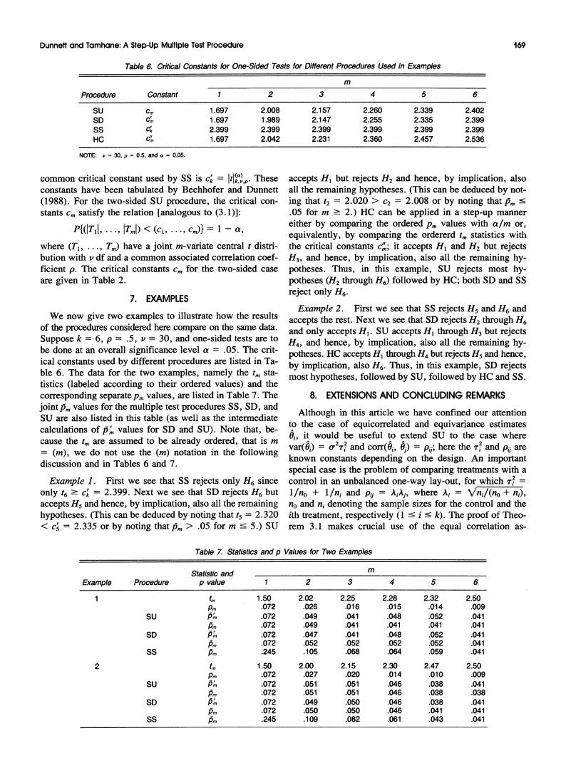
Table 6. Critical Constants for One-Sided Tests for Different Procedures Used in Examples

m

Procedure Constant 1 2 3 4 5 6

SU cm 1.697 2.008 2.157 2.260 2.339 2.402 SD cm 1.697 1.989 2.147 2.255 2.335 2.399 Ss ck 2.399 2.399 2.399 2.399 2.399 2.399 HC Cm 1.697 2.042 2.231 2.360 2.457 2.536

NOTE: v = 30, p = 0.5, and a = 0.05.

common critical constant used by SS is ck = ItI(a),. These constants have been tabulated by Bechhofer and Dunnett (1988). For the two-sided SU procedure, the critical constants cm satisfy the relation [analogous to (3.1)]:

P{(1T11, ..., I'mI) < (C1, . ., Cm)} = 1 - a,

where (T1, ..., Tm) have a joint m-variate central t distribution with v df and a common associated correlation coefficient p. The critical constants cm for the two-sided case are given in Table 2.

7. EXAMPLES

We now give two examples to illustrate how the results of the procedures considered here compare on the same data. Suppose k = 6, p = .5, v = 30, and one-sided tests are to be done at an overall significance level a = .05. The critical constants used by different procedures are listed in Ta- ble 6. The data for the two examples, namely the tm statistics (labeled according to their ordered values) and the corresponding separate pm values, are listed in Table 7. The joint Pm values for the multiple test procedures SS, SD, and SU are also listed in this table (as well as the intermediate calculations of Pmi' values for SD and SU). Note that, because the tm are assumed to be already ordered, that is m = (m), we do not use the (m) notation in the following discussion and in Tables 6 and 7.

Example 1. First we see that SS rejects only H6 since only t6 > Ck = 2.399. Next we see that SD rejects H6 but accepts H5 and hence, by implication, also all the remaining hypotheses. (This can be deduced by noting that t5 = 2.320

<c' = 2.335 or by noting that im > .05 for m s 5.) SU

accepts H1 but rejects H2 and hence, by implication, also all the remaining hypotheses. (This can be deduced by noting that t2 2.020> c2 = 2.008 or by noting that Pm s .05 for m 2 2.) HC can be applied in a step-up manner either by comparing the ordered pm values with a/rm or, equivalently, by comparing the ordererd tm statistics with the critical constants c"; it accepts H1 and H2 but rejects H3, and hence, by implication, also all the remaining hypotheses. Thus, in this example, SU rejects most hypotheses (H2 through H6) followed by HC; both SD and SS reject only H6.

Example 2. First we see that SS rejects H5 and H6 and accepts the rest. Next we see that SD rejects H2 through H6 and only accepts H1. SU accepts H1 through H3 but rejects H4, and hence, by implication, also all the remaining hypotheses. HC accepts H1 ftrough H4 but rejects H5 and hence, by implication, also H6. Thus, in this example, SD rejects most hypotheses, followed by SU, followed by HC and SS.

8. EXTENSIONS AND CONCLUDING REMARKS

Although in this article we have confined our attention to the case of equicorrelated and equivariance estimates Oi, it would be useful to extend SU to the case where var(6) = (2 v and corr(61, 6) = P1j; here the ?i- and pij are known constants depending on the design. An important special case is the problem of comparing treatments with a control in an unbalanced one-way lay-out, for which Ti = 1/no + 1/ni and pij = AiAj, where Ai = V/ni/(no + n1), no and ni denoting the sample sizes for the control and the ith treatment, respectively (1 s i ' k). The proof of Theo- rem 3.1 makes crucial use of the equal correlation as-

Table 7. Statistics and p Values for Two Examples

Statistic and m Example Procedure p value 1 2 3 4 5 6

tm 1.50 2.02 2.25 2.28 2.32 2.50 Pm .072 .026 .016 .015 .014 .009

SU Pm .072 .049 .041 .048 .052 .041 PAm .072 .049 .041 .041 .041 .041

SD Pm .072 .047 .041 .048 .052 .041 Pm .072 .052 .052 .052 .052 .041

SS Pm .245 .105 .068 .064 .059 .041

2 tm 1.50 2.00 2.15 2.30 2.47 2.50 Pm .072 .027 .020 .014 .010 .009

SU Pm ~ .072 .051 .051 .046 .038 .041 uPm .072 .051 .051 .046 .038 .038

SD Pm .072 .049 .050 .046 .038 .041 Pm .072 .050 .050 .046 .041 .041

SS Am .245 .109 .082 .061 .043 .041


sumption. If the theorem is true in the unequal correlation case, then a different proof must be found. The computing of the ci for this case would have to be done specifically for each problem. The probability expression to be computed would be as in Equation (3.3) but with di = (ci + Aizo)/I1 - Ai2 (1 ? i ? k). Alternatively, approximate values of the ci could be computed by using the arithmetic average of the Pij between the Oi still left to be tested. Whether the resulting approximation is conservative would require investigation.

Finally we note that, whereas the uniform improvement in power that was found to occur when the step-up modi- fication of the Bonferroni procedure due to Hochberg (1988) was used instead of the step-down modiflcation due to Holm (1979) may have suggested that step-up procedures have some inherent power advantage, we have found from our comparison of the two approaches under normal theory that the step-up testing has a nonnegligible power advantage only in those situations where most hypotheses are false and it is desired to reject all of them. This power advantage increases with the number of false hypotheses. But our comparison under normal theory also has revealed that even in situations where only a few hypotheses are false, the step- up test procedure stands at only a negligible power disadvantage with respect to the step-down test procedure.

[Received May 1990. Revised December 1990.]

REFERENCES

Bechhofer, R. E., and Dunnett, C. W. (1988), "Tables of Percentage Points of Multivariate Student t Distributions," in Selected Tables in Mathematical Statistics, 11, Providence, RI: American Mathematical Society, pp. 1-371.

Bechhofer, R. E., and Tamhane, A. C. (1981), "Incomplete Block De- signs for Comparing Treatments With a Control: General Theory," Technometrics, 23, 45-57.

Canner, S. G., and Walker, W. M. (1982), "Baby Bear's Dilemma: A Statistical Tale," Agronomy Journal, 74, 122-124.

Duncan, D. B. (1965), "A Bayesian Approach to Multiple Compari- sons," Technometrics, 7, 171-222.

Duncan, D. B., and Dixon, D. 0. (1983), "k-ratio t Tests, t Intervals, and Point Estimates for Multiple Comparisons," in Encyclopedia of Statistics (vol. 4) eds. S. Kotz and N. L. Johnson, New York: John Wiley, pp. 403-410.

Dunnett, C. W. (1955), "A Multiple Comparison Procedure for Com-

paring Several Treatments With a Control," Journal of the American Statistical Association, 50, 1096-1121.

Dunnett, C. W., and Tamhane, A. C. (1990), "A Step-up Multiple Test Procedure," Technical Report 90-1, Northwestern University, Dept. of Statistics.

(1991), "Step-Down Multiple Tests for Comparing Treatments With a Control in Unbalanced One-way Layouts," Statistics in Medi- cine, 10, 939-947.

Finner, H., Roters, M., and Hayter, A. J. (1991), "On the joint distribution function of order statistics with reference to step-up multiple test procedures," manuscript submitted for publication.

Hayter, A. J., and Tamhane, A. C. (1990), "Sample Size Determination for Step-Down Multiple Test Procedures: Orthogonal Contrasts and Comparisons With a Control," Journal of Statistical Planning and In- ference, 27, 271-290.

Hochberg, Y. (1988), "A Sharper Bonferroni Procedure for Multiple Tests of Significance," Biometrika, 75, 800-802.

Hochberg, Y., and Tamhane, A. C. (1987), Multiple Comparison Pro- cedures, New York: John Wiley.

Holm, S. (1979), "A Simple Sequentially Rejective Multiple Test Pro- cedure," Scandinavian Journal of Statistics, 6, 65-70.

Hommel, G. (1988), "A Stagewise Rejective Multiple Test Procedure Based on a Modified Bonferroni Test," Biometrika, 75, 383-386.

Marcus, R., Peritz, E., and Gabriel, K. R. (1976), "On Closed Testing Procedures With Special Reference to Ordered Analysis of Variance," Biometrika, 63, 655-660.

Miller, R. G., Jr. (1966), Simultaneous Statistical Inference, New York: McGraw-Hill.

Naik, U. D. (1975), "Some Selection Rules for Comparing p Processes With a Standard," Communications in Statistics, Part A-Theory and Methods, 4, 519-535.

O'Brien, P. C. (1983), "The Appropriateness of Analysis of Variance and Multiple Comparison Procedures," Biometrics, 39, 787-788.

O'Neill, R. T., and Wetherill, G. B. (1971), "The Present State of Mul- tiple Comparisons Methods" (with discussion), Journal of Royal Sta- tistical Society, Ser. B, 33, 218-241.

Perry, J. N. (1986), "Multiple-Comparison Procedures: A Dissenting View," Journal of Economic Entomology, 79, 1149-1155.

Rom, D. M. (1990), "A Sequentially Rejective Test Procedure Based on a Modified Bonferroni Inequality," Biometrika, 77, 663-665.

Rothman, K. J. (1990), "No Adjustments Are Needed for Multiple Com- parisons," Epidemiology, 1, 43-46.

Scheffe, H. (1953), "A Method of Judging All Contrasts in the Analysis of Variance," Biometrika, 40, 87-104.

Tukey, J. W. (1953), The Problem of Multiple Comparisons, unpub- lished manuscript, Princeton University, Dept. of Statistics.

Waller, R. A., and Duncan, D. B. (1969), "A Bayes Rule for Symmetric Multiple Comparisons," Journal of the American Statistical Associa- tion, 80, 1484-1503.

Welsch, R. E. (1977), "Stepwise Multiple Comparison Procedures," Journal of the American Statistical Association, 72, 566-575.

Westfall, P. H., and Young, S. S. (1989), "p Value Adjustments for Multiple Tests in Multivariate Binomial Models," Journal of the Amer- ican Statistical Association, 84, 780-786.

a step-up multiple test procedure - northwestern...

Documents