a stacked delta-nabla self-adjoint problem of even orderfaculty.cord.edu/andersod/p26_mcm.pdf · a...

MATHEMATICAL

coMPIJTEx MODELLING

PERGAMON Mathematical and Computer Modelling 38 (2003) 481-494 www.elsevier.com/locate/mcm

A Stacked Delta-Nabla Self-Adjoint Problem of Even Order

D. R. ANDERSON Department of Mathematics and Computer Science, Concordia College

Moorhead, MN 56562, U.S.A. andersodQcord.edu

J. HOFFACKER Department of Mathematics, University of Georgia

Athens, GA 30602, U.S.A. johoffQmath.uga.edu

(Received December 2002; revised and accepted May 2003)

Abstract-Existence criteria for two positive solutions to a nonlinear, even-order stacked delta, nabla boundary value problem with stacked, vanishing conditions at the two endpoints are found using the method of Green’s functions. A few examples are given for standard time scales. The corresponding even-order nabla-delta problem is also discussed in detail. @ 2003 Elsevier Ltd. All rights reserved.

Keywords-Time scales, Boundary value problem, Fixed points. Cone, Green’s function

1. INTRODUCTION

In this paper, we determine the Green’s function for a self-adjoint, even-order boundary-value problem, namely,

Bx=h, where Bx := (-1)” (x”“)~~,

with the boundary conditions

xAS(u) = 0, O<i<n--1,

( > XAn ‘O’ (b) = 0,

(1) O<i<n-1,

on a time scale T, where a E T and b E T”” with (~“(a) < pn(b), x : [u,a”(b)] -+ B, and h : [a, b] -+ Iw is a given Id-continuous function. Very little has yet been done on time-scale problems of higher order using the method of Green’s functions. Recently, Anderson [l] has considered an n-point right focal problem with delta derivatives, and Hoffacker has looked at delta-based problems such as the focal problem with stacked boundary conditions at the two endpoints [2], and for a (Ic, n - Ic) problem (31. Chyan, Henderson and Pan [4] have worked with

0895-7177/03/$ - see front matter @ 2003 Elsevier Ltd. All rights reserved. doi: lO.lOlS/SO895-7177(03)00244-g

Typeset by .AJ,@-T@

482 D. R. ANDERSON AND J. HOFFACKER

even-order, delta-derivative, Sturm-Liouville conditions. Even less attention has been focused, however, on mixing delta and nabla derivatives in higher-order derivative operators. Atici and Guseinov [5] broke ground on the problem for order two, but it has been unclear as to how to place the successive derivatives beyond second order. Our motivation for this work is to begin an extension of the self-adjoint problem first suggested in [5, p. 761, by stacking the delta derivatives first, followed by nabla derivatives; as is evident in (l), the boundary conditions are also stacked. Because the delta and nabla derivatives do not commute for the general time scale, one might also consider some alternating scheme in the differential operator. Anderson and Hoffacker [6] have considered one possibility, alternating nabla-delta, nabla-delta or delta-nabla, delta-nabla for an even-order operator; in that case, the boundary conditions at the two endpoints alternated as well, resulting in a different, though somewhat related, problem. As one might expect, the technique of finding the corresponding Green’s function for the related homogeneous case has proven to be an effective method in most of these problems. Throughout this work, we assume a working knowledge of time scales and time-scale notation. In the next section, however, we summarize the main points in a quick review.

2. TIME-SCALE ESSENTIALS

Any arbitrary nonempty closed subset of the reals lR can serve as a time scale T, see [7,8].

DEFINITION 1. For t E T, define the forward jump operator c : ‘I + % by

o(t) = inf{s E T : s > t}

and the backward jump operator p : T -+ T by

p(t) = sup{s E T : s < t}.

It is convenient to have the graininess operators pO, p,, : T + [0, oo) defined by p,,(t) = a(t) - t and /+(t) = p(t) - t.

DEFINITION 2. A function f : ‘I’ + W is right-dense continuous (rd-continuous) provided it is continuous at all right-dense points of T and its left-sided limit exists (finite) at left-dense points of ‘II’. The set of all right-dense continuous functions on T is denoted by

Similarly, a function f : T --t lR is left-dense continuous (Id-continuous) provided it is continuous at all left-dense points of Vi’, and its right-sided limit exists (finite) at right-dense points of T. The set of a11 left-dense continuous functions is denoted

Cld = Cld(T) = Cld(T,R)*

Define the sets T, and T” by

T = 7w7mL 1

if % has a right-scattered minimum m2, n

T, otherwise.

Tn = T - {ml) 7 if T has a left-scattered maximum ml

T, otherwise,

In addition, use the notation ‘Pa = (F)“, etc.

A Stacked Delta-Nabla Self-Adjoint Problem 483

DEFINITION 3. DELTA DERIVATIVE. Assume f : T -+ lR is a function and let t E ‘IT”. Define fA(t) to be the number (provided it exists) with the property that given any E > 0: there is a neighborhood U c ‘IT oft such that

\[f(a(t)) - f(s)] - fA(t)[o(t) - s]( 5 +(t) - s/, for all s E U.

The function fA (t) is the delta derivative of f at t.

DEFINITION 4. DELTA INTEGRAL. Let f : T t lR be a function, and a, b E T. If there exists a function F : T + R such that FA(t) = f(t) f or all t E T, then F is a delta antiderivative of f . In this case, the integral is given by the formula

s ab EAT- = F(b) - F(a), for a, b E T.

DEFINITION 5. NABLA DERIVATIVE. For f : T + R and t E ‘II’,, define f”(t) to be the number (provided it exists) with the property that given any E > 0, there is a neighborhood U oft such that

(f(p(tN - f(s) - P(t>b(t) - sl( I +G) - 4 for aJJ s 6 U.

The function fv (t) is the nabla derivative off at t.

In the case T = R, fA(t) = f’(t) = fV(t). When T = Z, fA(t) = f(t + 1) - f(t) and f”(t) = f(t) - f@ - 1).

DEFINITION 6. NABLA INTEGRAL. Let f : % t R be a function, and a, b E T. If there exists a function F : II’ -+ R such that FV(t) = f(t) f or all t E ‘II’, then F is a nabla antiderivative off. In this case, the integral is given by the formula

/ ab fog = F(b) - F(a), for a, b E ‘II’.

REMARK 7. All right-dense continuous functions are delta integrable, and all left-dense continuous functions are nabla integrable.

3. GREEN’S FUNCTION

We now initiate the process of constructing and analyzing the Green’s function for Bx = 0 with boundary conditions (1). The following two standard lemmas are easily verified.

LEMMA 8. The homogeneous boundary value problem Bx = 0, (l), has only the trivial solution.

LEMMA 9. The nonhomogeneous boundary value problem

Bx = h.

xAi(a) = cq, O<iln-1,

( > XAn v’ (b) = Pi, Oli<n--1,

where (pi, pi E Iw for 0 5 i 5 n - 1 and h is a given Id-continuous function, has a unique solution.

Define the Cauchy function for this boundary value problem as follows.

484 D. R. ANDERSON AND .J. HOFFACKER

DEFINITION 10. The function y : [u,a”(b)] x [a, b] + II% is the Cauchy function for Bx = 0 provided for each fixed s E [a, b], y(., s) is the solution to the initial value problem

BY(., s) = 0,

yA”(s, s) = 0, Oliin-1, (2)

Y *” ( > v’ (s, s) = 0, OIi_<n-2, (3)

( > Y *- vn-1 (s,s) = (-1)“. (4

REMARK 11. In order to make calculations with the Cauchy and Green’s functions simpler, define the functions gj,k : [a, c?(b)] x [a, b] -+ lR for j, Ic 2 0 recursively by

go,o(h s) 5 1,

t Sj,o(G s) = s

s gj-l,o(v)V~,

gj&, s) = s

t gj,k-1 (7, SW. s

Note that go,l(t, s) = gl,o(t, s) = t - s since the nabla and delta antiderivatives of a constant are equal. If j, Ic < 0, then gj,k(t, s) is taken to be identically zero. The construction of these functions is motivated by similarly defined functions for the delta case [2,3,7,9] and the nabla case [8,10].

EXAMPLE 12. For T = R, it is easy to see that

gj,k(t, s) = ct - ++lc (jtk)! ' for j, k 2 0. For T = Z, however, we find that

So,o(C s) = 1,

g&t, s) = v,

gO,k(t, s) = y,

g,k(t s)= (t-s+.i-w 3, 7 (j+k)! ’

j LO,

k > 0,

j _> 1, k L 0,

l)(t - 2). . . (t - m + where t? := t(t + l)(t + 2). . . (t + j - 1) and t” := t(t -

EXAMPLE 13. For T = qNo, we find that 1).

So,o(C s) = 1,

j-1 tqi _ s Sj,o(hS) = fJ - ,

i=o lb qr t-=0

k-1 t - qis go,rc(t, s> = n 7’ i=” rgo4’

g,k(t s)= @+S) (&-+) 3, 7 j+k-1 i

’

j 20,

j, k 2 1.


LEMMA 14. The Cauchy function for Ba: = 0 is (-l)ngn-l,n(t, s).

PROOF. By definition, g,-i,n(.,s) satisfies Bgn-l,n(.r s) = 0 for any fixed s E [a,b]. Thus, it only remains to show that gn-i,n( +, s) satisfies the initial values (2)-(4). For 0 5 i 2 n .. 1,

so (-l)ng,-i,n(t, s) satisfies the initial conditions (2). In addition, for 0 5 i 5 n - 2.

((-l)ngn41,n) v’ (4 s) = (-l)ngn-l-i,o(4 s),

so the initial conditions (3) are satisfied. For condition (4), note that

(4 s> = (-l)ngo.o(t, s) = (-lY>

which completes the proof. I

REMARK 15. In the proof of the next theorem, it is useful to note that, for 0 5 i < n --. 2,

since

I P(t)

sn-i,O(&>, t) = gn-1-i,o(T, tjv.T

= P;(t)g-,o(t, t) = 0.

THEOREM 16. For each fixed s E [a, b], let u(t, s) be the unique solution of the boundary value problem

Bu=O,

uAZ (a: s) = 0, O<iln-1, c-3

( > 7LA” 17' (hs) = -(-l)"gn-14,0(4s), O<i<n--1. (6)

Then the Green’s function G : [u,a”(b)] x [a,b] -+ IR for Bz = 0, (I), is given by

G(t, s) = 4t, s), t 5 s,

4t> s) + (-~)ngn-l,n(t, s), s I t. (7)

PROOF. Since for each fixed s E [u,b], u(.,s) and (-l)ng,-i,,(.,s) are solutions of Bz = 0, we have that, for each fixed s E [a, b],

v(t7 s) := 4t, s) + (-l)ng7L-l,n(t, s) (8)

is also a solution of Ba: = 0. It follows from (6) that for each fixed s E [a, b], v(., s) satisfies the boundary conditions at b for 0 < i < n - 1.

Let h be a given left-dense continuous function on [a, b], and define

s b z(t) := G(t, s)h(s)Vs.

a


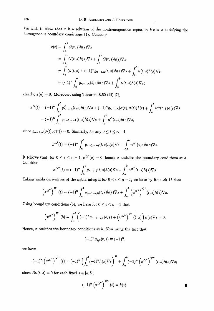
We wish to show that x is a solution of the nonhomogeneous equation Bx = h satisfying the homogeneous boundary conditions (1). Consider

I b

x(t) = G(t: s)h(s)Vs a

= J t

G(t, s)h(s)Vs + a s

b

G(t, s)h(s)Vs t =

I a kt, s) + (-1)%-l,&, s))h(s)Vs + lb+, s)h(s)Vs

= (-lJn J’gn-l,n(t, s)h(s)Vs + /-bu(t. s)h(s)Vs; a a

clearly, z(u) = 0. Moreover, using Theorem 8.50 (iii) [7],

J t

xA(t) = (-1)” b

d&(4 44)Vs + (-l)%-,&(t), o(t))h(t) + I uA(t, s)h(s)Vs

a a

= (-l)n /-tgn-l,n-l(t, s)h(s)Vs + /buA(t,s)h(s)Vs, a a

since gn-l,n(a(t), a(t)) = 0. Similarly, for any 0 5 i < n - 1,

zag(t) = (-1)” 1” gn-l,n-i(t, s)h(s)Vs + /buAi(t, s)h(s)Vs. a a

It follows that, for 0 .I i I n - 1, xA”(o) = 0, hence, x satisfies the boundary conditions at a. Consider

xA” (t) = (-1)” s’gn-l,o(t, s)h(s)Vs + lb uA” (t, s)h(s)Vs. a a

Taking nabla derivatives of the nabla integral for 0 5 i 5 n - 1, we have by Remark 15 that

(x”“) ” (t) = (-l)n /‘gn-1-i,o(t, s)h(s)Vs + 1” (u”“)” (t, s)h(s)Vs. a a

Using boundary conditions (6), we have for 0 I i 5 n - 1 that

(x”“)“’ (b) = 1” ((-1)%,x-l-i,o(b, s) + (u”“)~’ (b, s)) h(s)Vs = 0. a

Hence, x satisfies the boundary conditions at b. Now using the fact that

(-m7o,o(t, s) E (-l)“,

we have

(-1)” (x”y (t) = (-1y (J’ a

(I)“hW’~) v + /b(-l)” (u”“)~* (t, s)h(s)Vs; a

since Bu(t, s) = 0 for each f!ixed s E [a, b],

(-1)” (zAn)vn (t) = h(t).


THEOREM 17. If

the Green’s function for the boundary value problem Bx = 0, (l), is given by (7)-

PROOF. By Theorem 16, it suffices to show that for each fixed s E [a, b], u(., s) satisfies the boundary value problem Bz = 0 with boundary conditions at a, and w(., s) in (8) satisfies the boundary conditions at b. Fix s E [a, b]. By the properties of determinants and the construction of gj,k(t, s), Bu(., s) = 0 and uA’(u, s) = 0 for 0 5 i 2 n- 1, for 21 as in (9). As a result, boundary conditions at a are satisfied for each fixed s E [a, b] by U( ., s) in (9). It remains to show that ‘u(., S) satisfies the boundary conditions at b. Now v(t, s) can be written in determinant, form as

gn-l,& s) go,& a) Sl,&, u) . . gn-2,n(tr u) gn-l,n(t, a)

gn-LO@, s) 1 g1,0(4 a) . . gn-2,0(4 a) gn-l,O(b, u:!

gn-2,0(4 s> 0 1 . .

v(t,s) = (-l)n gn-3,o(h a> gn-2.0(4 4

. . .

I

it is easy to see that

and that

( > wAn I71 (t, s)

g1,0(4 s) 0 0 . 1 gl,o(~~ al 1 0 0 . 0 1

gn-l-i,o(t, 3) go-i,o(4 a) g1-i,O(h a) . . . gn-2-i,0(t, u) gn-~-qJ(t, u) gn-l,O(b, s> 1 Sl,O@, a) . . . &2,0(4 a) gn-l,O(h a)

gn-2,0(4 s) 0 = (-1)" . .

1 . . .

* Sl,O@, s) 0 0 . . . 1 Sl,O(h a) 1 0 0 . . 0 1

for 1 5 i 5 n - 1 (recalling that if the subscript on the function g is less than 0: the function is taken to be identically 0). For each such i, the first and (i + 2)nd rows will be identical, and hence, (~~*)~‘(b, s) = 0 for 0 5 i < n - 1. Therefore, the boundary conditions at b are likewise satisfied. I EXAMPLE 18. There has been some question as to whether the stacking of rr delta derivatives followed by n nabla derivatives, as in the self-adjoint dynamic equation, would lead to a svmmetric


Green’s function for the corresponding boundary value problem Bs = 0, (1). Unfortunately, we cannot expect the Green’s function to be symmetric. Take T = Z. For n = 2,

and

44 s) = u(t, s> + 91,2(t, s)

= &s - u)(s -a + 1)(3t - s - 2a - 2).

Notice that G(t, s) # G(s, t).

EXAMPLE 19. Similarly, one may find the Green’s function for the case ‘I’ = q”o where n = 2. Here

u(t7 s> = go,z(t, +?l,O(b, 4 - 91,2@, a> - So,z(C &71,0@, s>

= (t - 4y-+c?;Hb - a) _ (t - a)(t - we - !I24 _ (t - a>(t - F)(b - 3)

(1+ 4)U + Q + q2) 1+q

= (t - a)(t - w>(s - a) _ (t - a>(t - w)(t - q24

1+q (1+ 4)P + 4 + cl21

and

v(t, s) = u(t, s) + L71,2(& s)

= (t - u)(t - qu)(s -a) _ (t - a)@ - qu)(t - q2u) + (t - s)(t - qs)(t - q24

1+q (1+ q)(l + 4 + q2> (1+ q)(l + 4 + q2)

and again G(t, s) # G(s, t).

LEMMA 20. Let G(t, s) be the Green’s function for the boundary value problem Bx = 0, (1). Then, the following hold.

(i) (-l)i(GA”)v’ (t, s) > 0, u<t<s<b,O<i<n-1. (ii) GA’@, s) > 0, t E (cPmi (a), b], s E (a, b], 0 < i 5 n - 1.

PROOF. By the previous theorem, the Green’s function for this boundary value problem is given by

G(t, s) = 1

u(t,s), t 5 s,

v(t, s), s 5 t,

where u and v are as given (9) and (8)) respectively.

PART (i). For t 5 s, G(t, s) = u(t, s). H ence, Part (i) is equivalent to showing that

(-l)i (uAn)V’ (t, S) > 0, u 5 t < s 5 b, 0 < i 5 n - 1.

In order to determine the sign of u(t, s) and its derivatives, we first consider w(t, s). Fix s E [a, b]. Since v(.,s) satisfies Bv(.,s) = 0, (vA”)““-l(t, s) is a constant. Considering the boundary condition at b, this gives that (~~“)““-~(t, s) zz 0, which in turn implies that (wan)““-‘(t, s) is


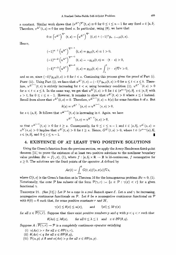
a constant. Similar work shows that (~l*“)~” (t, s) z 0 for 0 5 i 5 n - 1 for any fixed s E [a, b]. Therefore, van (t,s) = 0 for any fixed s. In particular, using (8), we have that

0 E wan ( )v’ (t, s) = (u”“)“’ (c s) + (-mLl-i,O(C s)

Hence,

(-1y-1 (u”n)vn-l (t, s) = go&, s) EE 1 > 0,

(qn-2 (uA”) v”-2 (t, s) = -g&, s) = -(t - s) > 0,

(-1y3 (u”“)vn-3 (t, s) = g2,0(t, s) = /‘(T - s)V7 > 0, s

and so on, since (-l)jgj,o(t, s) > 0 for t < s. Continuing this process gives the proof of Part (i).

PART (ii). Using Part (i), we have that uAn(t, s) = (-1)7Lg12,0(t, s) > 0 for a < t < s 5 b. There- fore, uAn-l (t, ) s is strictly increasing for t < s; using boundary condition (l), u*“-’ (t, s) > 0 for a < t < s 5 b. In the same way, we get that u*‘((t,s) > 0 for t E (~~-~(a), b], s E [a, b] with s > t, for 0 5 i 5 n - 1. However, it remains to show that w*‘(t, s) > 0 where s 2 t instead. Recall from above that w*” (t, s) = 0. Therefore, v *“-‘(t, s) = k(s) for some function k of s. But

k(s) = v*~-~(s, s) = u*--’ (s, s) > 0,

for s E (a, b]. It follows that vAnp2 (t, s) is increasing in t. Again, we have

?F-* (s, s) = tr2 (3, s) > 0,

SO that v*“-*(t, s) > 0 for t 2 s. Consequently, for 0 5 i 5 71 - 1 and t E [s, b], uA’(.s, s) = u*‘(s,s) > 0 implies that vAi(t,s) > 0 for t 2 s. Hence, G*‘(t,s) > 0, where t E (~9-~(a),b], s E (a, b], and 0 5 i 5 R. - 1. I

4. EXISTENCE OF AT LEAST TWO POSITIVE SOLUTIONS

Using the Green’s function from the previous section, we apply the Avery-Henderson tied-point theorem [ll] to prove the existence of at least two positive solutions to the nonlinear boundary value problem Bx = f(., IC), (l), where f : [a, b] x JR -+ Iw is Id-continuous, f nonnegative for x 2 0. The solutions are the fixed points of the operator A defined by

s

b

dx(t) = G(t, s)f(s, x(s))Vs>

where G(t, s) is the Green’s function as in lheorem 16 for the homogeneous problem Bz = 0, (1). Notationally, the cone P has subsets of the form P(r,r) := {x E P : y(x) < r) for a given functional y.

THEOREM 21. (See (111.) Let P be a cone in a real Banach space E. Let cy and y be increasing, nonnegative continuous functionals on P. Let 9 be a nonnegative continuous functional on P with 0(O) = 0 such that, for some positive constants r and M,

r(x) I@(x) I a(x), and IIXII I M-f(x)

for all x E P(r, r). Suppose that there exist positive numbers p and q with p < q < r such that

Q(Xx> i qx), for all 0 5 X < 1 and x E aP(O,q).

Suppose A : P(-y, r) -+ P is a completely continuous operator satis@ing

(i) y(Ax) > r for all x E aP(y,r), (ii) B(Az) < q for all x E dP(d,q),

(iii) P(a,p) # 0 and a(Ax) > p for all x E dP(cx,p).


Then A has at least two fixed points XI and 22 such that

P < 0 ($1) 7 with 0(x1) < q and 4 < 0 (x2), with 7(x2) < T.

Let & denote the Banach space Gld[pn(u), g”(b)] with the norm

By Lemma 20, G(t,s) > 0 for t E (an(a),b], s E (a,b], and GA(t,.s) > 0 for t E (~“-~(u),b], s E (a,b]. Let 71 E (a”(a),b). Then

0 < G(q, s) I G(t, s) I G(h s>,

for all s E (a,b], t E [q,b]. Set Gh 4 C:= min -,

44 G(4 s) (10)

(If a 5 s < q < b, then G(q,s)/G(b,s) = v(r,~,s)/v(b, ) s , and any (s - u) factors would cancel, leaving C well defined.) Clearly, 0 < f? < 1 and

lG(b, s) I G(t, s) I G(h s>,

for all t E [v, b], s E [a, b]. Define the cone P C E by

z is nonnegative on [a, b],

z P=

is nondecreasing on [a, b],

z is positive on (a”(a), b], x E E, (11)

x(t) 2 WI7 t E h%

where e is given in (10). To accomplish that which follows, we will need the constants

J b

,-1 .- .- G(b, s)Vs (12) a

and

J b

k-l := e G(b, s)Vs. (13) 9

Finally, let the nonnegative, increasing, continuous functionals y, 8, and o be defined on the cone P by

r(x) := &niibl x(t) = x(77),

e(x), cY(x) := r&,x(t) = x(b)*

Observe that, for each x E P, -dx) I e(x) L 44

and llxll = x(b) 5 +x(q) = $(z) 5 is(x) = +(x).

(14)

(15)


THEOREM 22. Let 1, m, and k be as in (IO), (12), and (13), respectively. Suppose there exist positive numbers p, q, and r such that

O<p<q<r,

and suppose an Id-continuous function f satisfies the following conditions: (i) f(s, W) 2. 0 for s E [a, b] and w E [0, r/l], (ii) f(s, w) > pk for s E [v, b] and w E [p,p/e],

(iii) f(s, w) < qm for s E [a, b] and w E [q, q/l], (iv) f(s, w) > rk for s E [q,b] and w E [r,r/i].

Then, the even-order boundary value problem Bx = f (., x), (l), has at least two positive solutions x1 and x2 such that

P < tg$l x1(t) < 4

and mm x2(t) > q, thbl

PROOF. Note that the Green’s function G(., s) is increasing by Lemma 20 on (Y+‘(a), b] and positive on (a“(a), b], for all s E (a, b]. Using the boundary conditions at a, G is nonnegative and nondecreasing for all (t, s) E [a, b] x [a, b]. F or 2 E P, x(t) 2 fJ/jx/j for all t E [7j,b]. Let t E [q,b]. Then

s

b

dx(t) = G(t, s)f(s, x(s>)Vs a

so that d(P) c P. For any x E P, (14) and (15) imply that

and

II41 5 -Y(Z). e It is clear that e(O) = 0, and for all x E P, X E [0, 11, we have

Since 0 E P and p > 0, P(cx,p) # 0. In the following claims, we verify the remaining conditions of Theorem 21. CLAIM 1. If x E aP(a,p), then cr(dz) > p. Since x E dP(cqp), p = IIxlI I p/e. Thus,

J b

cy(dx) = max WA a

Gtt, s)f(s, x(s))Vs

J b

= G(4 s)f(s, x(s>)Vs a

L J b (74 s)f(s, x(s))Vs 7 L e J b G(h s)f(s, x(s)>Vs II

J b

> pke G(b, s)Vs ?

= P, by Hypothesis (ii) and (13).


CLAIM 2. If 2 E dp(O,q), then B(dz) < q. Note that z E dP(O,q) and (15) imply that Q = II4 F q/e.

s b

= G(4 s)f(s, x(s>)Vs a

b

< qm J

G(b, s)Vs a

= Q,

by Hypothesis (iii) and (12).

CLAIM 3. If 2 E W(y,r), then r(dz) > r. Since 2 E dP(y,r), from (15) we have that min,!+$] z(t) = T and T 5 llzll 5 s.

J b

r(h) = t;Fbl G(t, 4fh x(s>>Vs ) a

J b

= G(v, s)f(s, x(s>>Vs a

2 e J

b G(4 s)f(s, x(s>)Vs 1)

J 6

_> rice G(b, s)Vs ‘I

= r,

by Hypothesis (iv), using arguments as in Claim 1. Therefore, the hypotheses of Theorem 21 are satisfied and there exist at least two positive fixed points q and 22 of A in P(r, r). Thus, the even-order boundary value problem Bz = f(., z), (l), h as at least two positive solutions 21 and 22 such that

P < Q,(Xl), with 0(x1) < q,

and

4 < f3 (x2) 7 with 7(x2) < T. I

5. A STACKED NABLA-DELTA SELF-ADJOINT PROBLEM

One may wonder if stacking the nabla and delta derivatives in the opposite order affects the symmetry of the Green’s function or the existence of positive solutions. In this section, we consider the self-adjoint even-order boundary value problem

cx = f, where Cx := (-1)” (z”“)~~,

with the boundary conditions

xVX(u) = 0, O<iln-1,

( > xv” A’ (16)

(b) = 0, O<iln-1,

on a time scale T, where a E Tnn and b E T with an(a) < p”(b), z : [p*(a), b] + R, and f : [a, b] + B is a given rd-continuous function. As in previous sections, we first develop the Green’s function and then use it to show the existence of a positive solution. Since the proofs are very similar to those already given, they are omitted here.


LEMMA 23. The homogeneous boundary value problem Cx = 0, (16), has only the trivial solution.

LEMMA 24. The nonhomogeneous boundary value problem

cx = f,

XV”(U) = cq, osi<n-1,

(X”“)*‘(b) = ,&, Oli_<n--1,

where ~i, ,L$ E If8 for 0 5 i < n - 1 and f is a given rd-continuous function, has a unique solution.

As before, we define the Cauchy function for this boundary value problem as follows.

DEFINITION 25. The function y : [~“(a),61 x [a,b] --+ R is the Cauchy function for Cz = 0 provided for each fixed s E [a, b], y(., s) is th e solution to the initial value problem

CYC.7 s) = 0, yqs, s) = 0, O<i<n-1,

*’ (s, s) = 0, O<i<n-2,

( ) Y V” *--I (s, s) = (-l)n

The auxiliary functions similar to gj,k are instead

hj,k : [P”(u), b] X [a, b] + R,

for j, k 2 0, defined recursively by

ho,ok s> = 1,

hj,o(t, s) = s

t

hj-l,o(T, sP-, 3

s

t

hj,/& s) = hj,k-l(c s)V7.

LEMMA 26. The Cauchy function for Cx = 0”i.s (-l)“h,-l,n(t, s).

THEOREM 27. For each fixed s E [a, b], let ~(t, s) be the unique solution of the boundary value problem

cu=o. uyu, s) = 0, O<i<n-1,

( > UVn *’ (b,s)= -(-l)ngn-l-i,0(b7s), OliFn-1.

Then the Green’s function G : [p”(a), b] x [a, b] -+ R for Cx = 0, (16), is given by

THEOREM 28. If

u(t, s) = (-1)n

G(t,s) = u(t, s), t 5 3, u(t, s) + (-lT‘h,-l,,(t, s), s i t.

0 ho,n(t, a> h,n(t, a> . . . hn-z,n(t, a> Ll,&. a> Ll,o(4 s> 1 hl,o(b, a) . . . Lz,o(b, a) hn-l,o(b, a> hn-2,o@, s) 0 1 . . hn-3,o@, a) L2,o(h a)

hl,oib, s) 0 0 . 1 hldb, aj 1 0 0 . . . 0 1

the Green’s function for the boundary value problem Cx = 0, (16), is given by (17).

(17)

>

As in Example 18, one may show that the Green’s function for the boundary value problem Cx = 0, (16) is not symmetric in general. In addition, the existence of two positive solutions of

Cx = f(.,x:>, (16) can be shown in a manner similar to that in Theorem 22.


REFERENCES 1. D.R. Anderson, Positivity of Green’s function for an n-point right focal boundary value problem on measure

chains, Muthl. Comput. Modelling 31 (6/7), 29-50, (2000). 2. J. Hoffacker, Green’s functions and eigenvalue comparisons for a focal problem on time scales, Advances in

Diference Equations IV, Special Issue of Computers Math. Applic. 45 (6-Q), 1339-1368, (2003). 3. J. Hoffacker, Green’s functions for higher order equations on time scales, PanAmerican Mathematical Journal

11 (4), l-28, (2001). 4. C.J. Chyan, J. Henderson, and Y.J. Pan, Eigenvalue intervals for 2mth order Sturm-Liouville boundary value

problems., J. Differ. Equations Appl. 8 (5), 403-413, (2002). 5. F.M. Atici and GSh. Guseinov, On Green’s functions and positive solutions for boundary value problems on

time scales, J. Comput. Appl. Math. 141 (l/2), 75-99, (2002). 6. D.R. Anderson and J. Hoffacker, Green’s function for an even order mixed derivative problem on time scales,

Dynamic Systems and Applications 12 (l/2), Q-22, (2003). 7. M. Bohner and A. Peterson, Dynamic Equations on Time Scales, An Introduction with Applications, Birk-

h&user, Boston, MA, (2001). 8. M. Bohner and A. Peterson, Advances in Dynamic Equations on Time Scales, Birkhiiuser, Boston, MA,

(2003). 9. R.P. Agarwal aud M. Bohner, Basic calculus on time scales and some of its applications, Results Math. 35

(l/2), 3-22, (1999). 10. D.R. Anderson, Taylor polynomials for nabla dynamic equations on time scales, PanAmerican Mathematical

Journal 12 (4) 17-27, (2002). 11. R.I. Avery and J. Henderson, Two positive fixed points of nonlinear operators on ordered Banach spaces,

Comm. Appl. Nonlinear Anal. 8, 27-36, (2001).

a stacked delta-nabla self-adjoint problem of even orderfaculty.cord.edu/andersod/p26_mcm.pdf · a...

Documents