3/17/2008 1

A SIMPLE THROW MODEL FOR FRONTAL VEHICLE-PEDESTRIAN COLLISIONS

Milan Batista University of Ljubljana

Faculty of Maritime Studies and Transportation Pot pomorščakov 4, SI- 6320 Portorož, Slovenia, EU

milan.batista@fpp.edu

ABSTRACT

This paper discusses a simple theoretical throw model for frontal vehicle-pedestrian collisions. The model is based on the simple assumption that pedestrian movement after impact can be approximated by movement of a mass point. Two methods of reconstruction of vehicle-pedestrian collision are discussed: one knowing only the throw distance and the other when also impact to ground contact distance is known. The model is verified by field data available in the literature and by comportment with full scale numerical simulation.

1 INTRODUCTION

The investigation of vehicle-pedestrian collisions must have begun in the middle of the sixties mainly for the purpose of accident reconstruction. From that time several models describing the motion of pedestrians after impact with vehicles was developed ([1],[2],[3],[4],[5],[6],[8],[9],[10],[11],[13],[14],[15],[17],[18]). Basically there are two types of models: theoretical, based on laws of mechanics, and empirical. Theoretical models yield reliable results; however, considerable input data from real world collisions is needed to solve the equations. On the other hand empirical models--usually consisting of a single regression formula which connects the vehicle impact speed with pedestrian throw distance ([5],[17])--need no particular data; however their application is limited only to well defined scenarios and the accuracy of models is within, say,

10km/h± ([7]). Typically the empirical models do not include road grade, which can be an influence factor when one determines vehicle impact velocity from throw distance. The hybrid models try to combine features of both basic models ([3]). In the present paper the model of frontal vehicle-pedestrian collision closely following the Han-Brach approach ([3],[6]) is developed. The details of derivation of equations are included for comprehensiveness. In addition to Han-Brach equations the equations for total flying time and total throw time and throw distance are also given. The basic equation of reconstruction--i.e., the equation for calculation of pedestrian launch velocity--is then obtained by inverting the equation for total throw distance. This equation is, in the special case of a horizontal road, reduced to the so called Searle equation ([15][16]). The four methods of reconstruction are then discussed: the method when one knows the pedestrian launch angle and friction between pedestrian and road; the Serale method ([15]) where the launch angle is estimated on the basis of extreme of

3/17/2008 2

launch velocity; and two new methods where in addition to throw distance the distance from impact to ground contact is also known.

2 THE MODEL

2.1 Assumptions

Only the frontal impact of the vehicle with the pedestrian is considered. In the case when the vehicle has enough speed or it is braking the pedestrian will, after impact, be thrown from the vehicle hood, fly through the air, impact the ground and then slide/roll/bounce on the ground to a rest. The possible impacts of pedestrian with the road obstacles in the last phase are excluded from consideration. To describe these events mathematically the following assumptions are made:

the car-pedestrian impact is symmetric so all events happens in a single plane the initial velocity of the pedestrian is zero after launch the pedestrian is considered as a mass point the ground is flat the pedestrian-ground friction is constant all air resistance is neglected

vC0

vP0

y

x

h

θ

s0

t0

s1

t1

s2

sP

tP

α

g

μ

Figure 1. Vehicle-pedestrian collision variables and events

According to events description and the above assumptions the following basic variables are included in the model (Figure 1):

gravity acceleration 29.8 m/sg = , mass of the vehicle Cm and mass of the pedestrian Pm , initial pedestrian launch height h (not pedestrian COG), total pedestrian throw distance Ps ; i.e., the distance the pedestrian travels from

impact to his rest position on the ground,

3/17/2008 3

total pedestrian throw time Pt , vehicle impact velocity 0Cv , pedestrian launch velocity 0Pv , road gradient angleα , pedestrian launch angle θ , coefficient of friction μ between the pedestrian and the ground.

It is further assumed that the total throw distance Ps and total throw time Pt can be expressed as the sum of three phases--contact phase, flying phase and sliding/rolling/bouncing phase ([4],[11]). The total throw distance is therefore 0 1 2Ps s s s= + + (1) and the total throw time is 0 1 2Pt t t t= + + (2) where indices 0, 1, 2 belong consecutively to impact, flying and sliding. 2.2 Contact phase

This phase roughly consists of ([4])

• vehicle-pedestrian contact • impact--i.e., acceleration of the pedestrian's body • movement on the vehicle's hood

In the scope of the present paper, the movement of the body onto the vehicle can be roughly of two types:

• wrap trajectory - here the pedestrian is wrapped over the front of vehicle , usually involving a decelerating vehicle

• forward projection - in this case COG of pedestrian is below the leading edge of the vehicle at impact

The main goal in this phase is to connect vehicle impact velocity 0Cv with pedestrian launch velocity 0Pv and also to determine the contact path length 0s and contact time 0t . This last is beyond the scope of this paper and therefore will not be discussed. However in the case of forward projection one can approximately take 0 0s = and 0 0t = . More detailed analysis of impact and future references can be found in [4], [6] and [18]. Despite the fact that this phase of throw influences others, only a simple model will be present: it is assumed that impact between vehicle and pedestrian is plastic. In this case

3/17/2008 4

from conservation of momentum--i.e., from ( )0 0C C C P Cm v m m u= + --the initial contact velocity of the vehicle 0Cv is

00 1

CC

P C

vum m

=+

(3)

where 0Cu is vehicle/pedestrian post impact velocity. The case of non-plastic impact is discussed in [8]. Because the velocity 0Cu and the pedestrian launch velocity 0Pv differ for the case of wrap trajectory, a coefficient η called pedestrian impact factor is introduced to relate them ([6][15][18]):

00 0 1

CP C

P C

vv um m

ηη= =+

(4)

In general the coefficient η can not be constant and it is in general dependant on various factors, including vehicle impact velocity, geometry of vehicle front, pedestrian height, etc. ([18]).

2.3 Flying phase

Following Figure 1 and Newton’s 2nd Law the equations of motion of pedestrian COG are the well known equation of a projectile in a vacuum:

sin

cos

xx P P

yy P P

dvdx v m m gdt dt

dvdy v m m gdt dt

α

α

= = −

= = −

(5)

where t is time, ,x y are coordinates of COG of pedestrian, and ,x yv v its velocity components. The equation is completed with the following initial conditions

( ) ( )

( ) ( )

0

0

0 0 0 cos

0 0 sin

x P

y P

x v v

y h v v

θ

θ

= =

= =

(6)

Carrying out the integration and imposing initial conditions one finds velocity 0 0cos sin sin cosx P y Pv v g t v v g tθ α θ α= − = − (7)

3/17/2008 5

and position coordinates

2 2

0 0cos sin sin cos2 2P Pt tx v t g y h v t gθ α θ α= − = + − (8)

At impact time 1t --i.e., the time when the pedestrian impacts the ground--the following conditions are reached: ( )1 0y t = and ( )1 1x t s= . From these, by using (7) and (8), one obtains the flying time

2 2

0 01

sin sin 2 coscos

P Pv v ght

gθ θ α

α+ +

= (9)

and the flying distance

21

1 0 1cos sin2Pts v t gθ α= − (10)

2.4 Impact with ground

At pedestrian impact with the ground the Newton dynamical equations take the following impulse form ( ) ( )y y y x x xm v v I m v v I+ − + −− = − = − (11) where superscripts + and – denote velocities before and after impact, and xI and yI are impulses in road horizontal and vertical direction, respectively. Here one needs further assumptions about the nature of impact. The simplest are:

• the impact is plastic--i.e., 0yv+ = • the Coulomb friction law is valid at impact--i.e., x yI Iμ=

On the basis of these assumptions one can from the first of (11) find impulse in vertical direction y yI mv−= − and from the second the horizontal velocity after impact

x x xv v I m+ −= − . From those, by using friction law, one obtains x x yv v vμ+ − −= + . By using (7) this becomes ( ) ( )0 1cos sin sin cosx Pv v g tθ μ θ α μ α+ = + − + (12)

3/17/2008 6

2.5 Sliding phase

After impact with ground the pedestrian slides to rest. The dynamical equations governing this motion are

sin 0 cosxx x y

dvdx v m mg N mg Ndt dt

α α= = − − = − + (13)

where xN and yN are horizontal and normal reaction of the ground, respectively, and the initial conditions are ( ) ( )0 0 0x xx v v+= = (14) By assuming that the Coulomb friction law is valid--i.e., x yN Nμ= --one, after integration and imposing the initial conditions obtain the velocity ( )sin cosx xv v g tα μ α+= − + (15) and the distance

( )2

sin cos2xtx v t g α μ α+= − + (16)

At the end of pedestrian sliding one has ( )2 0xv t = and ( )2 2x t s= . From these, by using (15) and(16), the sliding time 2t is

( )2 sin cos

xvtg α μ α

+

=+

(17)

and the sliding distance 2s is

( )

( )

2

2 2 sin cosxv

sg α μ α

+

=+

(18)

2.6 Total throw time and throw distance

The total time and distance can be, after calculation, obtained by summing the times and distance of flying and sliding phase. However it turns out that a simple formula exists. That is, by substituting (12) into (17) one obtains the total pedestrian throw time Pt

3/17/2008 7

( )

( )0

0

cos sinsin cos

PP

vt t

gθ μ θ

α μ α+

= ++

(19)

and by introducing (19) into (17) one finds the total throw distance

( )( )

220

0

cos sin2 sin cosP

P

vs s h

gθ μ θ

μα μ α

+= + +

+ (20)

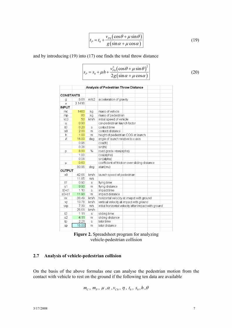
Figure 2. Spreadsheet program for analyzing

vehicle-pedestrian collision

2.7 Analysis of vehicle-pedestrian collision

On the basis of the above formulas one can analyse the pedestrian motion from the contact with vehicle to rest on the ground if the following ten data are available Cm , Pm , μ ,α , 0Cv , η , 0t , 0s , h ,θ

3/17/2008 8

Among these the last five can in practice only be estimated. Nevertheless since all the equations describing the collision are algebraic and explicit they can be easily implemented into a spreadsheet program. An example of that is shown by Figure 2. The data used in the example of Figure 2 will be used in all the following examples.

3 RECONSTRUCTION

In the reconstruction of pedestrian accidents one usually knows the throw distance and asks for launch velocity on which vehicle impact speed can be estimated. Two cases will be considered: the case of known throw distance and the case where the flying distance is also known. 3.1 Known throw distance

If the pedestrian throw distance Ps is known, then from (20) one can express pedestrian launch velocity

( )( )0

0

2 sin coscos sin

PP

g s s hv

α μ α μθ μ θ

+ − −=

+ (21)

By denoting tanp α≡ (22) the formula (21) can be written in the following form

( )( )( )

( )

20

0 24

2 1 tan

1 tan 1

PP

g p s s hv

p

μ θ μ

μ θ

+ + − −=

+ + (23)

The confidence analysis of the formula is given in Appendix A. For 0p = and 0 0s = one obtains the Searle formula ([15]). If the pedestrian launch velocity 0Pv is known, the vehicle impact velocity is, from (4)

( ) 00 1 P

C P Cvv m mη

= + (24)

The formulas (23) and (24) can be used for reconstruction of vehicle-pedestrian collision if the following data are available Cm , Pm , η , μ , p, Ps , 0s , h ,θ

3/17/2008 9

The spreadsheet program for reconstruction of vehicle-pedestrian collision on the basis of (23) and (24) is shown in Figure 3. Note that by taking throw distance 16 m and data from the previous example, the impact velocity of the vehicle is 50 km/h, as it should be.

Figure 3. Spreadsheet program for reconstruction of a

vehicle-pedestrian collision Before proceeding, the effect of grade on pedestrian launch velocity will be discussed in some details. Let ( )0 0 ,P Pv v α θ= . In the special case of no grade--i.e., 0α = --eq (21) becomes

( ) ( )00

20,

cos sinP

P

g s s hv

μ μθ

θ μ θ− −

=+

(25)

The quotient of (21) and (25) is ( )( )

0

0

,sin cos

0,vv

α θα μ α

θ= + and is independent of θ

so one can define normalized launch velocity

( )2

,1

pu pp

αμμ

μ+

≡+

(26)

3/17/2008 10

The diagram of (26) for various values of μ is shown in Figure 4.

Now it follows that ( ),0 1uα μ = and ( ) 1lim ,0p

uα μμ→∞

= . Thus if 1μ ≤ then if the

pedestrian is launched uphill--i.e., if 0p > --then the launch velocity for reaching the distance Ps is greater than that of horizontal ground; while if 1μ > this is true only for

grades satisfying 2

21

p μμ

≤−

. But since the grades of the roads are limited to

approximately 0.3p < and the friction coefficient is limited approximately to 2μ < this limit can practically never be reached. In the case of downhill launch--i.e. for 0p < --one should have pμ > − in order that the pedestrian can attain the rest position and in this case the launch velocity for reaching the distance Ps is lesser than that of horizontal ground.

-2 -1 0 1 2 3 40.0

0.2

0.4

0.6

0.8

1.0

1.2

1.4

1.6

0.5 1.0

u α=v

0(α,θ

)/v0(0

,θ)

p

1.5

Figure 4 Effect of grade on normalized launch velocity for various values of μ

3.2 Known throw distance - Searle method

The difference between grade p of the road and the angle θ in Eq (23) is practical: while the grade of the road can be measured, the launch angle θ can only be estimated. Here it was Searle’s idea that the formula (23) can be used to determine lower and upper boundaries, by considering the launch angle θ that will minimize and maximize the expression ([15]). Therefore the effect of launch angle on pedestrian launch velocity will now be considered.

3/17/2008 11

First, for horizontal launch--i.e., for 0θ = --eq (21) reduces to ( ) ( )( )0 0,0 2 sin cos Pv g s s hα α μ α μ= + − − (27)

The quotient ( )( )

0

0

, 1,0 cos sin

P

P

vv

α θα θ μ θ

=+

is independent of grade angle α so one can

introduce the normalized launch velocity

( ) 1,cos sin

uθ μ θθ μ θ

≡+

(28)

The graph of this function for various values of μ is shown in Figure 5

0 15 30 45 60 75 900.4

0.6

0.8

1.0

1.2

1.4

1.6

1.8

2.0

u θ=v0(α

,θ)/v

0(α,0

)

θ [deg]

μ = 0.0

0.2

0.4

0.6

0.8

1.01.2

1.41.6

Figure 5 Normalized launch velocity as function of launch angle for various values of friction coefficients

Since the launch angle is limited to 02πθ≤ < the two limits of the functions are

( ),0 1uθ μ = and 1,2

uθπμ

μ⎛ ⎞ =⎜ ⎟⎝ ⎠

. Now, if 1μ > then it follows from (28) that

( ), 1uθ μ θ < . The function in this case reaches its maximum at 0θ = . Thus the maximal velocity for reaching the distance Ps is obtained at 0θ = and its value is

( ) ( ) ( )0max 0 *2

2 11

P

pv g s s h

p

μμ μ θ θ

+= − − > ∨ ≤

+ (29)

3/17/2008 12

For 1μ ≤ one sees from Figure 6 that ( ) ( )*,0 , 1u uθ θμ μ θ= = where *θ is the critical launch angle ([15]) given by

* 2

2arctan1

μθμ

=−

The expression (29) is thus valid only for *θ θ≤ . If *θ θ> then the maximal velocity

obtained for the launch angle is 2πθ → with

( ) ( ) ( )0max 0 *2

1 2 11

P

pv g s s h

p

μμ μ θ θ

μ+

< − − ≤ ∧ >+

(30)

Now as can be seen from the graph of Figure 3 the velocity given by (28) has a

minimum. The minimum is obtained from the condition 0dud

θ

θ= , which gives ([15])

tanθ μ= (31) For this value of angle, the function has minimal value

min 2

11

uθμ

=+

(32)

But since for 0μ > one has min 1uθ < it follows that ( ) ( )0 0, ,0v vα θ α< . The minimal velocity for reaching the given distance ps is thus

( ) ( )

( )0

0min 2 2

2

1 1pg p s s h

vp

μ μ

μ

+ − −=

+ + (33)

The above formulas generalize the Searle formulas ([15]) in a way that they include road grade and contact distance. They provide means to estimate velocity bounds if throw distance is known. The spreadsheet program for reconstruction of vehicle-pedestrian collision based on these formulas is shown by Figure 6. Note that if one considers the example in Figure 2 as a reference, the Searle method estimates the impact velocity between 48.3 km/h to 56.3 km/h, while the 'true' value is 50 km/h.

3/17/2008 13

Figure 6 Spreadsheet program for reconstruction of a

vehicle-pedestrian collision by the Searle method.

3.3 Known flying and throw distance

In a case when besides throw distance the flying distance of the pedestrian is also known - for example from physical evidence - we can calculate both launch angle and launch velocity. If *s is impact to ground contact distance then the flying distance is 1 * 0s s s= − (34) From (10) and (9) one can express the flying time

( )( )

11

2 sin coscos cos sin sin

s ht

gθ θ

α θ α θ+

=−

(35)

and the pedestrian launch velocity

( ) ( )( ) ( )

2

0 1 21

1 tan

2 tan 1 tan 1

gv s ph

s h p p

θ

θ θ

+= +

+ − + (36)

Remark. The launch angle for minimal velocity of (36) is

3/17/2008 14

( )( ) ( )2 2 2

1 1

1

1tan

s h p h ps

s phθ

+ + − −=

− (37)

Since the pedestrian launch velocity is also given by (21) one can--by equating (36) and (21)--find the compatibility equation

( ) ( ) ( )( )( )

( )( )

2 21 1

20

1 tan 4 tan 1 tan

1 P

s p h p s h p

p s s h

μ θ μ θ θ

μ

+ + = + + −

× + − − (38)

From this either θ or μ can be calculated. In each of the cases the above relation reduces to a quadratic equation.

Figure 7. Results of calculation of vehicle-pedestrian collision.

Known impact to ground contact distance with estimated μ . Given μ . For a given μ one can arrange (38) to the following quadratic for unknown launch angle θ 2tan tan 0A B Cμ μ μθ θ+ + = (39) where

3/17/2008 15

( ) ( ) ( )

( )( ) ( )( ) ( )( )

( ) ( ) ( )

22 21 0 1 0 1

2 2 20 1 0 1 1 1

21

2 2 20 1 0

4 4

4 4 2 4

4

4 4 4

p P

p p

p P

A p s s s ps s s ph s ph

B p s s s ph s s s ph s phs p h

h s ph

C ph s s s ph h s s ph h

μ

μ

μ

μ μ

μ

μ

μ μ

= − − − − − − −

⎡ ⎤= − − + − − − + −⎣ ⎦− −

= − − + + − − −

(40)

The spreadsheet program for reconstruction of vehicle-pedestrian collision based on equation (39) is shown in Figure 7.

Given θ . On the other hand, for given θ one can arrange (38) to the quadratic equation for an unknown μ 2 0A B Cθ θ θμ μ+ + = (41) where

( )( )( ) ( )

( )( )( )( )( )( )( ) ( )

( )( )( )( ) ( )

22 21 1

21 0

221 1

221 0 1

4 tan 1 tan 1 tan

4 tan 1 tan 1

4 1 tan tan 1 2 tan

4 1 1 tan tan

P

P

A h s h p p s p h

B s h p p s s

ph p s h p h s p h

C p p p s h s s s p h

θ

θ

θ

θ θ θ

θ θ

θ θ θ

θ θ

= + − + + +

= − + − + −

+ − + + + +

= − + − + − + +

(42)

Since the launch angle θ can practically only be estimated the case is interesting for the extremes, which give maximum and minimum value of launch velocity. The first maximum value is forward projection. So, if 0θ = then from (41)

( )( )0 1 0 1 0 2

2P P Ps s ph s s s s s s ph

hμ

− − ± − − + − += (43)

This formula has h, which is usually small compared to Ps , in denumerator, so one can expect that it is very sensitive to its variation. The other extreme for maximal projection

velocity is 2πθ = . In this case (41) reduces to

( ) ( )2 2 2

1 1 14 4 0P Ps ph ps s hp p s sμ μ− + − + = (44)

3/17/2008 16

However this equation does not have any positive roots for 0p > .

Figure 8. Results of calculation of vehicle-pedestrian collision. Searle method with

known flying distance.

Now by taking tanθ μ= for minimum launch velocity then the quadratic equation (41)transforms to the quadratic equation of the form 4 3 2

0 1 2 3 4 0a a a a aμ μ μ μ+ + + + = (45) where

( )( ) ( )

( ) ( ) ( )( ) ( )

( ) ( )

20 1

21 1 1 0

2 2 22 1 1 1

2 23 1 0

24 1 0

4 1 4

4 1 2 4 2 2

4 1 4

4

P

P

P

a s hp

a h p s ph ps s s

a h p s ph s s ph p h

a h ps p h s s ph

a s hp ph s s

= −

⎡ ⎤= − − + −⎣ ⎦⎡ ⎤= − + + + + −⎣ ⎦

⎡ ⎤= − + − − +⎣ ⎦

= + − −

(46)

3/17/2008 17

The roots of this equation can be calculated numerically by the Newton iteration method. The example of the spreadsheet program implementing the above formulas is shown in Figure 8. The estimated boundary for data from Figure 1 are 45 km/h to 49 km/h. The first maximal value of vehicle impact velocity is calculated by using (29) and calculated μ for minimum value of vehicle impact velocity. The horizontal launch based on (43) gives the unrealistic friction coefficient 1.99 which leads to the upper velocity limit 93 km/h. Here one can recommend that in general the maximal value of vehicle impact velocity based on (43) can be used in the cases when the values of μ are, say, 1.1μ < .

4 VERIFICATION

4.1 Comportment with field data

The first comportment is made for test data given in [4]. The test was performed by a vehicle of mass 1542 kg. Since the mass of the pedestrian was not reported a value of 80 kg was taken into calculation. Results of the calculation using the Searle method are shown in Table 1. Note the huge discrepancy of calculated and measured vehicle impact velocity for Test no 69, performed by an non-braking vehicle. All other results are within acceptable limits of 15%.

Tabela 1. Results of calculation on test data [4]. Searle method. ( 0 2ms = , 0.95η = , 1.1mh = , 0.6μ = ) *Brake off

Input Output

Test no.

[ ]0

km/hCv

[ ]mPs[ ]

0min

km/hCv

[ ]0max

km/hCv

[ ]0

km/hCv

[ ]%Err

65 32.2 7.9 27.96 32.61 30.29 5.95 67 48.3 13.4 38.27 44.63 41.45 14.18 68 48.3 17.4 44.28 51.64 47.96 0.70 69* 64.4 61.9 86.51 100.89 93.70 -45.50 72 48.3 20.7 48.69 56.78 52.74 -9.18

For verification of the reconstruction method where besides the pedestrian throw distance are known the impact to ground is also known are given in [12]. The lack of data--the result of a real pedestrian accident--is that there is no mass of vehicle and pedestrian included in the report and that the vehicle impact velocity is below 36 km/h. The mass 1500 kg for vehicle and 80 kg for pedestrian was thus assumed in calculation. Results of comportment are shown in Table 2. It can be seen from the table that in trail case 1 the calculated velocity overestimates the impact velocity by about 25 %, and in case 2 the calculated values underestimate the velocity by about 50 %. In the other four cases the calculated impact velocity is between calculated limits within an error maximum of 13 %.

3/17/2008 18

Tabela 2. Comportment with field data [12]. Values marked with * are not included in calculation of 0maxCv . ( 1η = , 0 1ms h= = )

Input Output

Trail No. [ ]

0

km/hCv

[ ]* ms [ ]mPs minμ maxμ [ ]

0min

km/hCv

[ ]0max

km/hCv

[ ]

0

km/hCv

[ ]%Err

1 26.99 8.23 10.38 0.50 1.70* 31.67 35.38 33.53 24.21 3 25.13 2.59 5.42 0.13 0.15 12.30 13.37 12.84 48.93 4 20.19 3.53 7.41 0.19 0.26 17.83 21.28 19.56 3.15 10 20.28 3.65 4.73 0.34 0.55 17.08 22.29 19.69 2.93 11 27.85 5.52 8.52 0.35 0.76 25.09 38.01 31.55 13.29 14 32.13 8.24 8.51 0.71 2.76* 30.13 36.96 33.55 4.40

4.2 Comportment with full scale numerical simulation

The full scale numerical simulation of vehicle-pedestrian collision was done by the PC-Crash 7.1 computer program. The following data was used:

• vehicle bumper height: 0.5 m • vehicle front height: 0.8 m • distance from vehicle front to windshield: 1.02 m • vehicle mass: 1460 kg. • coefficient of tire-road friction: 0.8 • coefficient of car-pedestrian friction: 0.2 • coefficient of road-pedestrian friction: 0.6 • coefficient of restitution for pedestrian impact: 0.1

The first numerical experiment was conducted for a pedestrian of mass 80 kg and height 1.83 m. The path and speed of COG of pedestrian torso for various impact speeds are displayed in Figure 9 and numerical values are given in Table 2.

0 5 10 15 20 25 30 350.0

0.5

1.0

1.5

2.0

2.5

3.0

20

7060

5040

y

x

30

0.0 0.5 1.0 1.5 2.0 2.5 3.0 3.5 4.00

10

20

30

40

50

60

70

20

70

6050

40

V p [km

/h]

t [s]

30

Figure 9. Path and time dependence of velocity for pedestrian torso COG

for various vehicle impact speed. Pedestrian height is 1.83 m and mass 80 kg. (scales of x and y are different)

3/17/2008 19

For comportment of results of numerical simulation with PC-Crash and the present model the calculated values given in Table 3 are taken as input to the present spreadsheets programs. Results of calculations are shown n Tables 4, 5, 6, 7 and 8. The results of analysis of throw distance are within 20%. Among reconstruction methods the Searle method is dominant with maximum error in impact vehicle velocity of about 6% (Table 6). When impact to ground distance is included in input data the error raises to about 9 % (Table 7). When using the Searle method with known impact to ground distance the error raises to about 20 % (Table 8).

Tabela 3. Results of simulation of vehicle-pedestrian collision with PC-Crash. for pedestrian of height 1.83 m and mass 80 kg

[ ]0

km/hCv

[ ]

0

km/hPv

0θ ⎡ ⎤⎣ ⎦ [ ]0 st [ ]0 ms [ ]mh [ ]* mt [ ]* ms [ ]mPs η

20 17.30 -44.16 0.79 2.72 0.39 - - - 0.92 30 24.96 -6.10 0.40 2.31 1.01 1.00 5.78 7.56 0.87 40 34.99 3.52 0.27 2.07 1.08 1.05 8.62 11.85 0.92 50 44.77 7.42 0.22 2.14 1.15 1.16 11.76 16.87 0.95 60 55.46 9.88 0.20 2.37 1.20 1.26 15.20 23.20 0.97 70 69.08 14.16 0.20 2.88 1.35 1.51 20.71 34.25 1.04

Tabela 4. Results of calculation of vehicle-pedestrian collision with present method for pedestrian of height 1.83 m and mass 80 kg

Input Output

[ ]0

km/hCv

η 0θ ⎡ ⎤⎣ ⎦ [ ]0 st [ ]0 ms [ ]mh[ ]

0

km/hPv

[ ]* mt [ ]* ms [ ]mPs

20 0.92 -44.16 0.79 2.72 0.39 30 0.87 -6.10 0.40 2.31 1.01 24.47 0.79 4.94 6.39 40 0.92 3.52 0.27 2.07 1.08 34.89 0.80 7.23 11.26 50 0.95 7.42 0.22 2.14 1.15 45.03 0.9 10.53 18.02 60 0.97 9.88 0.20 2.37 1.20 55.18 1.03 14.91 26.72 70 1.04 14.16 0.20 2.88 1.35 69.02 1.39 24.96 42.60

Tabela 5. Comportment of results from Table 3 and 4.

Relative error in % for various variables

0Pv *t *s Ps

1.96 21.00 14.53 15.48 0.29 23.81 16.13 4.98 0.58 22.41 10.46 6.82 0.50 18.25 1.91 15.17 0.09 7.95 20.52 24.38

3/17/2008 20

Tabela 6. Results of simulation of vehicle-pedestrian collision for pedestrian of height 1.83 m and mass 80 kg. Searle method. ( 0 2ms = , 0.95η = ,

1.1mh = , 0.6μ = )

Input Output

[ ]0

km/hCv

[ ]mPs[ ]

0min

km/hCv

[ ]0max

km/hCv

[ ]0

km/hCv

[ ]%Err

30 7.56 26.03 30.36 28.20 6.02 40 11.85 35.65 41.57 38.61 3.48 50 16.87 44.33 51.70 48.02 3.97 60 23.20 53.30 62.15 57.73 3.79 70 34.25 66.10 77.08 71.59 2.27

Tabela 7. Results of simulation of vehicle-pedestrian collision.

for pedestrian of height 1.83 m and mass 80 kg. Known impact to ground distance. ( 0 2ms = , 0.95η = , 1.1mh = , 0.6μ = )

Input Output

[ ]0

km/hCv

[ ]* ms [ ]mPs[ ]

0

km/hCv

[ ]%Err

30 5.78 7.56 29.14 2.95 40 8.62 11.85 37.51 6.64 50 11.76 16.87 45.94 8.84 60 15.20 23.20 55.16 8.77 70 20.71 34.25 68.53 7.15

Tabela 8. Results of simulation of vehicle-pedestrian collision for pedestrian of height

1.83 m and mass 80 kg. Searle method. ( 0 2ms = , 0.95η = , 1.1mh = )

Input Output

[ ]0

km/hCv

[ ]* ms [ ]mPs μ [ ]

0min

km/hCv

[ ]0max

km/hCv

[ ]0

km/hCv

[ ]%Err

30 5.78 7.56 0.37 22.95 24.48 23.715 20.95 40 8.62 11.85 0.42 32.32 35.02 33.67 15.83 50 11.76 16.87 0.44 40.70 44.42 42.56 14.88 60 15.20 23.20 0.43 48.73 53.13 50.93 15.12 70 20.71 34.25 0.42 59.85 65.01 62.43 10.81

The second numerical experiment was conducted for vehicle impact velocity 60 km/h with various pedestrians. The following pedestrian height/mass pairs were used for calculation: 1.2/25, 1.4/40, 1.6/60, 1.83/80. The results of the calculations are shown in Figure 10 and results of calculation are given in Table 9. Note that the pedestrian of height 1.25 m is subject to forward projection while all others follow wrap trajectory.

3/17/2008 21

The comportment with results of calculation shows similar discrepancies as in the previous case (Table 10 and 11).

0 5 10 15 20 25 30 35 400.0

0.5

1.0

1.5

2.0

2.5

3.0

1.6

1.83

1.4

y

x

1.2

0.0 0.5 1.0 1.5 2.0 2.5 3.0 3.5 4.00

10

20

30

40

50

60

70

80

1.4

1.6

1.83

1.2

Vp [k

m/h

]

t [s] Figure 10. Path and speed of COG of pedestrian torso for various height of pedestrian.

Vehicle impact speed 60 km/h.

Tabela 9. Results of simulation of vehicle-pedestrian collision with PC-Crash. for vehicle collision velocity 60 km/h for various pedestrians

[ ]mPh [ ]

0

km/hPv

0θ ⎡ ⎤⎣ ⎦ [ ]0 st [ ]0 ms [ ]mh [ ]* mt [ ]* ms [ ]mPs η

1.25 70.39 12.94 0.22 3.74 1.49 1.34 21.96 36.30 1.19 1.40 63.38 8.74 0.21 3.18 1.24 1.18 17.24 30.55 1.09 1.60 57.81 12.15 0.20 2.60 1.27 1.33 16.76 25.61 1.00 1.83 55.46 9.88 0.20 2.37 1.20 1.26 15.20 23.20 0.97

Tabela 10. Results of simulation of vehicle-pedestrian collision with present method.

for various pedestrian at 60 km/h

Input Output

[ ]mPh η 0θ ⎡ ⎤⎣ ⎦ [ ]0 st [ ]0 ms [ ]mh[ ]

0

km/hPv

[ ]* mt [ ]* ms [ ]mPs

1.25 1.19 12.94 0.22 3.74 1.49 70.2 1.37 25.66 44.36 1.40 1.09 8.74 0.21 3.18 1.24 63.66 0.85 17.97 34.88 1.60 1.00 12.15 0.20 2.60 1.27 57.63 1.16 17.58 29.89 1.83 0.97 9.88 0.20 2.37 1.20 55.90 1.04 15.16 27.34

Tabela 11. Comportmant of results between Table 9 and 10.

Relative error in % on various variables

0Pv *t *s Ps

0.27 2.24 16.85 22.20 0.44 27.97 4.23 14.17 0.31 12.78 4.89 16.71 0.79 17.46 0.26 17.84

3/17/2008 22

5 CONCLUSION

The vehicle-pedestrian collision is a complicated event which can not be exactly modeled. The simple model present in this paper is comparable with the empirical models and tested full scale model within an error of, say, 20%. The model has the advantage over empirical models when the road has a grade or when the pedestrian impact to ground contact distance is available as data. The model can therefore be used for reconstruction purposes; however, one should be aware of its limitations and accuracy. All present spreadsheet programs are available from www.fpp.edu/~milanb/pedestrian

REFERENCES

[1] R.Aronberg. Airborne Trajectory Analysis Derivation for Use in Accident Reconstruction. SAE Technical Paper Series 900367.

[2] J. C. Collins. Accident Reconstruction. Charles C. Thomas Publisher, Springfield, Illinois, USA, 1979, pp. 240-242.

[3] R.M.Brach, R.M.Brach. Vehicle Accident and Reconstruction Methods. SAE International, 2005

[4] J. J. Eubanks, W. R. Haight. Pedestrian Involved Traffic Collision Reconstruction Methodology. SAE Technical Paper Series 921591.

[5] T.F.Fugger Jr., B.C.Randles, J.L.Wobrock, J.L.Eubanks. Pedestrian Throw Kinematics In Forward Projection Collisions. SAE Technical Paper 2002-01-0019.

[6] I. Han, R. M. Brach. Throw Model For Frontal Pedestrian Collisions. SAE Technical Paper Series 2001-01-0898.

[7] A.Happer, M.Araszewski, A.Toor, R.Overgaard, R.Johal. Comprehensive Analysis Method for Vehicle/Pedestrian Collisions. In: Accident Reconstruction, SAE SP-1491, 2000

[8] R.Limpert. Motor Vehicle Accident Reconstruction and Cause Analysis. 5th Edition. Lexis Publishing, Charlottesville, Virginia, USA, 1999. pp 539-554

[9] R.R.McHenry. B.G.McHenry. Occupant Trajectory. In: McHenry Accident Reconstruction 2000. McHenry Software, Cary, NC, USA, 200, pp.95-102.

[10] A.Moser, H.Steffan, G.Kasanicky. The Pedestrian Model in PC-Crash – The Introduction of Multi Body System and its Validation. SAE Technical Paper Series 1999-01-0445

[11] A.Moser, H.Hoschopf, H.Steffan, G.Kasanicky. Validation of the PC-Crash Pedestrian Model. SAE Technical Paper Series, 2000-01-0847

3/17/2008 23

[12] B.C.Randles, T.F.Fugger, J.J.Eubanks, E.Pasanen. Investigation and Analysis of Real-Life Pedestrian Collisions. SAE Technical Paper Series, 2001-01-0171

[13] C.G.Russell. Equations & Formulas for the Traffic Accident Investigators and Reconstructionist. Lawyers & Judges Publishing, Tuscon, AZ, USA, 1999

[14] H.Schnider. G.Beier. Experiment and Accident: Comparison of Dummy Tests Results and Real Pedestrian Accidents. SAE Tecnhical Paper Series 741177.

[15] J.A.Searle, A.Searle. The Trajectory of Pedestrians, Motorcycles, Motorcyclists, etc. Following a Road Accident. SAE Technical Paper Series 831622

[16] J.A.Searle. The Physics Of Throw Distance In Accident Reconstruction. SAE Technical Paper Series 930659.

[17] A.Toor, M.Araszewski. Theoretical Vs. Empirical Solutions For Vehicle/Pedestrian Collisions. 2003-01-0883, Accident Reconstruction 2003, Society of Automotive Engineers, Inc., Warrendale, PA, 2003, pp. 117-126.

[18] D.P.Wood. Application Of A Pedestrian Impact Model To The Determination Of Impact Speed. SAE Technical Paper Series 910814.

3/17/2008 24

APPENDIX A - Confidence analysis for Eq (21) To estimate the errors in parameters that influence the pedestrian launch velocity Eq (21) is viewed as a function of six variables ( )0 0, , , , ,P Pv f h s s p μ θ= (47) The excepted value of this function is ( )0 0, , , , ,P Pv f h s s α μ θ= (48) where 0, , , , ,Ph s s α μ θ is the given or measured values of variables. The coefficient of variation in the result 0Pv is estimated as

( ) ( ) ( ) ( ) ( ) ( )0 0

22 2 22 2

P Pv h h s s s s p pc f c f c f c f c f c f cθ θ μ μ= + + + + + (49)

where kc are the estimated coefficients of variation in k-th variable and kk

k

fff

ξξ

∂=

∂ are

dimensionless sensitivity coefficients whose explicit expressions are

( )02h

P

h f hff h s s h

μμ

∂⎛ ⎞= = −⎜ ⎟∂ − −⎝ ⎠ (50)

( )02P

P Ps

P P

s sfff s s s hμ

⎛ ⎞∂= =⎜ ⎟∂ − −⎝ ⎠

(51)

( )0

0 0

0 02sP

s sfff s s s hμ

⎛ ⎞∂= = −⎜ ⎟∂ − −⎝ ⎠

(52)

( )( )2

12 1p

p f p pff p p p

μμ

⎛ ⎞∂ −= =⎜ ⎟∂ + +⎝ ⎠

(53)

tan1 tan

fffθθ θ μθ

θ μ θ∂ −⎛ ⎞= =⎜ ⎟∂ +⎝ ⎠

(54)

( ) ( )( )( )( )( )

0 0

0

2 2 tan2 1 tan

P P

P

s s p h p s s p hfff p s s hμ

μ μ μ θμ μμ μ μ μ θ

− − + − + − −⎡ ⎤ ⎡ ⎤⎛ ⎞∂ ⎣ ⎦ ⎣ ⎦= =⎜ ⎟∂ + − − +⎝ ⎠ (55)