a simple proof the alternation - caltechauthorsauthors.library.caltech.edu/20456/1... · asimple...

A Simple Proof of the Alternation Theorem

P. P. VaidyanathanDept. of Electrical Engineering

California Institute of TechnologyPasadena, CA 91125

Email: [email protected]

Abstract-A simple proof of the alternation theoremfor minimax FIR filter design is presented in this paper.It requires no background on mathematical optimizationtheory, and is based on easily understood properties offilters with equiripple behavior. The method is similarto the classical counting argument used in early math-ematics literature. The contribution here is a simplifiedpresentation which directly uses filter design language.'

I. INTRODUCTIONThe McClellan-Parks method based on the Remez ex-

change algorithm has been used for the design of equirippleFIR filters for more than thirty years [1], [3]-[8]. A discussionof the method is included in nearly all well-known signalprocessing texts. The algorithm is based on a result calledthe alternation theorem which gives a set of conditions underwhich a filter design is optimal in the minimax sense. Thistheorem is therefore at the heart of the method. In signalprocessing texts this theorem is ususally not proved, but areference is given to mathematical optimization texts suchas [2]. The purpose of this paper is to provide a simpleproof which can be presented in the classroom and requiresno background on mathematical optimization theory. Theargument will be based on the simple fact that a polynomialof order M cannot have more than M zeros. Similar proofsbased on counting arguments were presented in old fashionedmathematics literature (e.g., [9] pages 56 and 61-62). Themain contribution in this paper is to present a proof directlyin filter-design language in a way that is simple and accessibleto readers with introductory signal processing background.

First some preliminaries. All discussions are restricted tothe case of linear phase real coefficient FIR filters. It is wellknown [6], [8] that there are four types of such filters. Type1 filters have the form

N

H(z) = : h(n) z-n=O

where N is even and

h(n) = h(N -n),

'Work supported in parts by the National Science Foundation grantCCF-0428326 and the California Institute of Technology.

T. Q. NguyenDept. of Electrical and Computer Engr.

University of CaliforniaSan Diego, CA 92093

Email: nguyentgece.ucsd.edu

so that [6], [8]

M

H(e-) = -jm E: bn cos(wn)n=O

where M = N12. The factor e- Nm representing the linearphase part will be ignored in all discussions. Since Type2, 3, and 4 filters can be expressed in terms of Type 1filters [8], the theory and design of linear phase filters iscentered around the design of the coefficients {bn} in the sumz;M bn cos(wn). This summation is used to approximatea real desired response D(w) in 0 < w < 7 with aspecified weighting function W(w) > 0 on the error. Theapproximation error is

M

E(w) = D(w) Z bncos(wn)n=O

whereas the weighted error of approximation is defined by

M

Eb(W) = W(w) [D(w) >jbn cos(wn)]n=O

call this B(w)

(1)

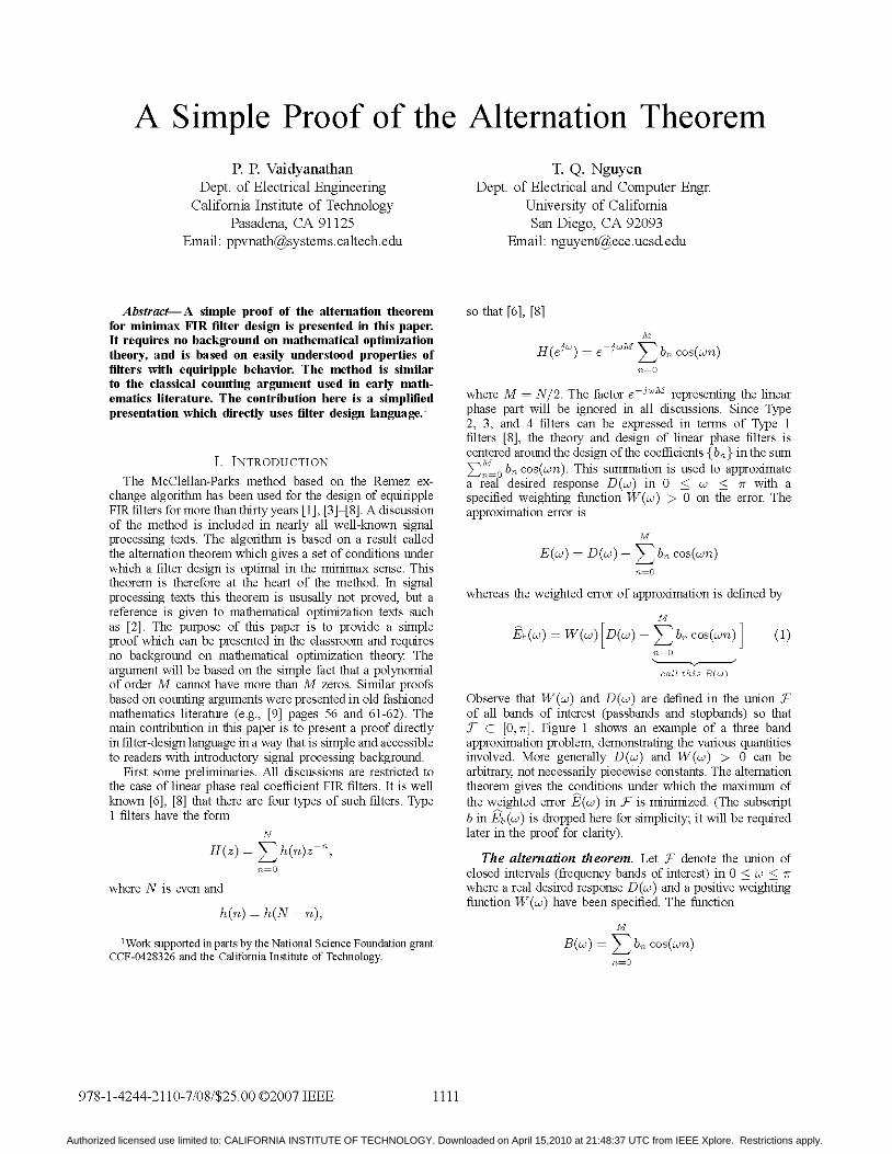
Observe that W(w) and D(w) are defined in the union Fof all bands of interest (passbands and stopbands) so thatF C [0, 7]. Figure 1 shows an example of a three bandapproximation problem, demonstrating the various quantitiesinvolved. More generally D(w) and W(w) > 0 can bearbitrary, not necessarily piecewise constants. The alternationtheorem gives the conditions under which the maximum ofthe weighted error E(w) in F is minimized. (The subscriptb in Eb (w) is dropped here for simplicity; it will be requiredlater in the proof for clarity).

The alternation theorem. Let .f denote the union ofclosed intervals (frequency bands of interest) in 0 < w < 7where a real desired response D(w) and a positive weightingfunction W(w) have been specified. The function

M

B(w) = Z bn cos(wn)n=O

978-1-4244-2110-7/08/$25.00 ©2007 IEEE 1111

Authorized licensed use limited to: CALIFORNIA INSTITUTE OF TECHNOLOGY. Downloaded on April 15,2010 at 21:48:37 UTC from IEEE Xplore. Restrictions apply.

is the unique weighted minimax approximation of D(w) inF with respect to the weighting function W(w) (i.e., B(w)minimizes the peak weighted-error IE(w) in F) if and onlyif there exist at least M + 2 distinct frequencies

WI < W2 ... < WM+2

(called extremal frequencies) in the set .f, satisfying twoproperties:

1) The weighted error E(w) alternates, that is,

E(wi) =-E(w2)= E(w3)

2) the maximum of IE(w) isfrequencies, that is,

maxIE(w)l =

for all k. <

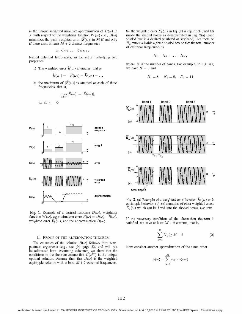
So the weighted error Eb(W) in Eq. (1) is equiripple, and fitsinside the shaded boxes as demonstrated in Fig. 2(a) (eachshaded box is a desired passband or stopband). Let there beNk extrema inside a given shaded box so that the total numberof extremal frequencies is

N1 + N2 + ... + NK,

where K is the number of bands. For example, in Fig. 2(a)we have K= 3 and

N1 = 8, N2 = 9, N3 = 14

attained at each of these

= JE(Wk)l,band 1 band 2 band 3

Eb (CO)(0

(a) -6

D(@o) 1

0

W(cO) 1

0

(o

It

desiredresponse

E(O))

Ea(co,) -(o

weight(o

(b)

(Derror

(O weightederror

approximation(o

Fig. 1. Example of a desired response D(w), weightingfunction W(w), approximation errro E(w) = D(w) -B(w),weighted error Eb (w), and the approximation B(w).

II. PROOF OF THE ALTERNATION THEOREM

The existence of the solution B(w) follows from com-

pactness arguments (e.g., see [9], page 23) and will notbe addressed here. Assuming existence, we show that theconditions in the theorem ensure that B(ed) is the uniqueoptimal solution. Assume then that B(w) is the weightedequiripple solution with at least M + 2 extremal frequencies.

E a(co)a

E(m

(C) -sopes

zero-slopes

Fig. 2. (a) Example of a weighted error function Eb (w) withequiripple behavior, (b), (c) examples of other weighted errorsEa (w) which can be fitted into the shaded boxes. See text.

If the necessary condition of the alternation theorem issatisfied, we have at least M + 2 extrema, that is,

K

Nk > M+2k=l

(0

(2)

Now consider another approximation of the same order

M

A(w) = an cos(nw)n=O

1112

<IAJV<

EI(O11 I II 11 11I0==L_I J v V IJ

B(co) \/M-/

0W v NPF 1-

;FA17-7


such that its peak error is at least as small as in the equiripplecase. That is, the weighted error

M

Ea (W) = W(w) [D(w) San cos(nw)]n=O

A(-v)

satisfiesmax Ea (W) < max Eb (w)

This means that Ea (w) also fits the shaded boxes as demon-strated by the thin curve in Fig. 2(b). We will show thenthat

A(w) -B(w) _ O,

that is, the two approximations are one and the same! Theargument will be based on the simple fact that a polynomialof order M has no more than M zeros. First observe thatsince Eb(w) swings between the two extreme values d and-6, the plot of Ea(w) intersects the equiripple plot Eb(w)at least Nk -1 times in the kth band. That is, the difference

AE(w)=Eb(w) -Ea(W)

has at least Nk -1 zeros in the kth band. For example thenumber of intersections in Fig. 2(b)are 7, 8, and 13. LettingNz be the number of zeros of AE(w) in 0 < w < 7, wetherefore have

K

Nz > E Nk - K.k=l

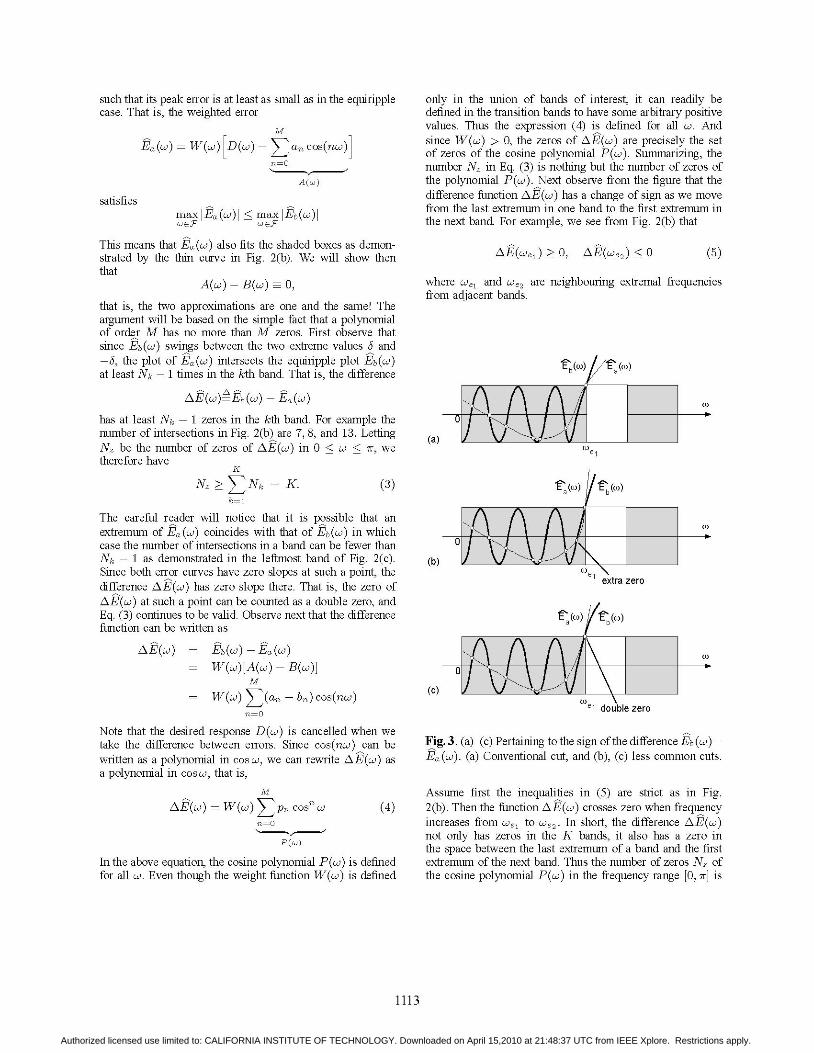
only in the union of bands of interest, it can readily bedefined in the transition bands to have some arbitrary positivevalues. Thus the expression (4) is defined for all w. Andsince W(w) > 0, the zeros of AE(w) are precisely the setof zeros of the cosine polynomial P(w). Summarizing, thenumber Nz in Eq. (3) is nothing but the number of zeros ofthe polynomial P(w). Next observe from the figure that thedifference function AE(w) has a change of sign as we movefrom the last extremum in one band to the first extremum inthe next band. For example, we see from Fig. 2(b) that

AE(we) > 0, AE(We2) < 0 (5)

where We1 and We2 are neighbouring extremal frequenciesfrom adjacent bands.

(a)

(3)

The careful reader will notice that it is possible that anextremum of Ea (w) coincides with that of Eb(w) in whichcase the number of intersections in a band can be fewer thanNk -1 as demonstrated in the leftmost band of Fig. 2(c).Since both error curves have zero slopes at such a point, thedifference AE(w) has zero slope there. That is, the zero ofAE(w) at such a point can be counted as a double zero, andEq. (3) continues to be valid. Observe next that the differencefunction can be written as

AE(w) = (Eb() -Ea(w)W(w)[A(w) -B(w)]

W(w) (an- bn) cos(nw)n=O

Note that the desired response D(w) is cancelled when wetake the difference between errors. Since cos(nw) can bewritten as a polynomial in cosw, we can rewrite AE(w) asa polynomial in cos w, that is,

M

AE(w) = W(w) E Pn cosn w (4)n=O

P(W)

In the above equation, the cosine polynomial P(w) is definedfor all w. Even though the weight function W(w) is defined

t (c)

(b)

co(0

(0

(0

extra zero

( ()o)

(c)

I \\I\

(0e1 double zero

Fig. 3. (a)-(c) Pertaining to the sign of the difference Eb (w)-Ea (w). (a) Conventional cut, and (b), (c) less common cuts.

Assume first the inequalities in (5) are strict as in Fig.2(b). Then the function AE(w) crosses zero when frequencyincreases from We1 to We2. In short, the difference AE(w)not only has zeros in the K bands, it also has a zero inthe space between the last extremum of a band and the firstextremum of the next band. Thus the number of zeros N, ofthe cosine polynomial P(w) in the frequency range [0, 7] is

1113

I.-,-,,,(co) /-EE b ((O)


K

K+K-=1 ZNk-1>M+1 (6)k=l

where the last inequality above follows from the assumptionthat are at least M + 2 extrema (see (2)). But we know thata polynomial of the form En- pnZx has only M zeros.

Setting x = cos w and observing that cos w is monotonicallydecreasing in 0 <w < 7 we conclude that P(w) cannot havemore than M zeros in 0 < w < 7. Equation (6) is thereforea contradiction of this unless P(w) is identically zero, thatis, Pn= 0 for all n. This means that B(w) = A(w) indeed.Summarizing, the weighted equiripple solution with at leastM + 2 extrema is the unique solution which minimizes themaximum weighted error.

If the intersection of Ea (w) and Eb (w) occurs right atthe band edge We1 we have AE(Wei) = 0. See Fig. 3(a).However, since P(w) is continuous, this still guarantees thatAE(Wei + e) > 0 for sufficiently small c. Thus AE(w)still has a zero-crossing between the last extremum of one

band and the first extremum of the next (in We1 <W <We2in the figure). The only exception to this argument wouldbe the two situations shown in Figs. 3(b) and 3(c). One iswhen Ea (w) cuts Eb (w) from the "wrong side" as in Fig.3(b). In this case an extra intersection or zero is generated as

demonstrated in the figure. The other is when the two error

plots are tangential at We1 (Fig. 3(c)) in which case we can

count the zero of AE(w) at We1 as a double zero. In eithersituation, therefore, the claim (6) continues to be true, and allarguments in the preceding paragraph continue to be valid.The proof is therefore complete. 7 7V7

III. CONCLUDING REMARKS

We conclude the paper with a number of important obser-vations pertaining to the above proof.

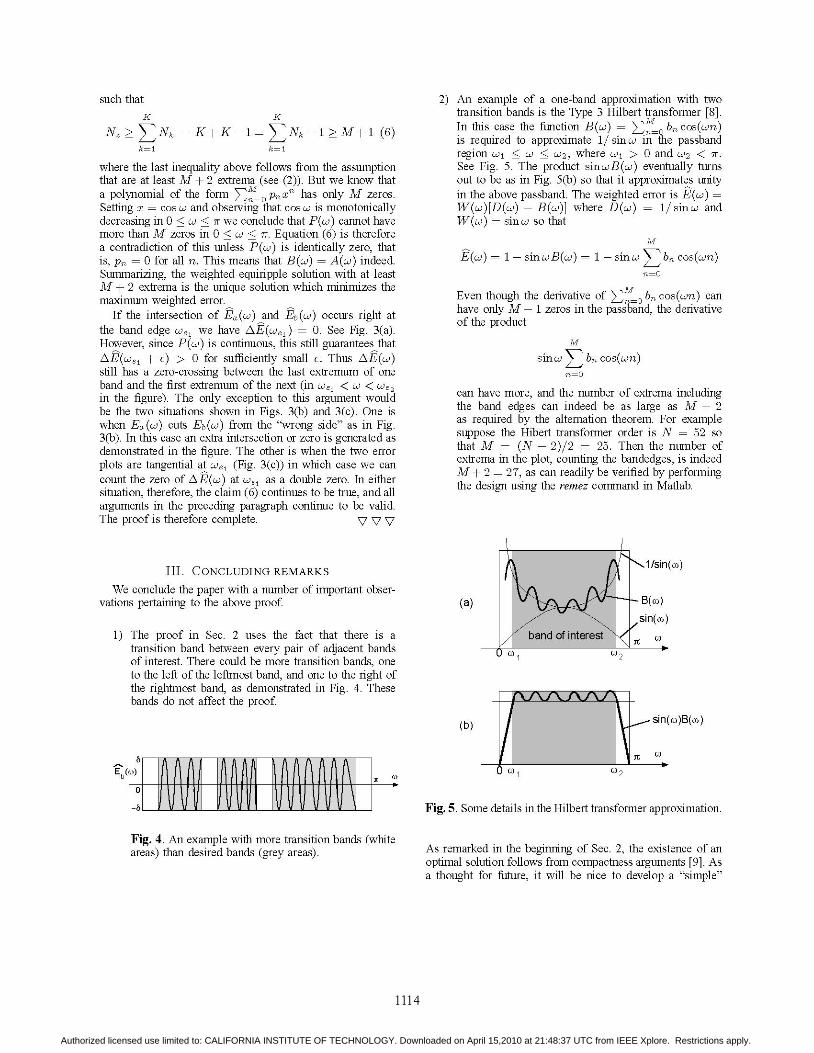
2) An example of a one-band approximation with twotransition bands is the Type 3 Hilbert transformer [8].In this case the function B(w) = Em bn cos(wn)is required to approximate 1lsinw in the passbandregion wi < w < W2, where wI > 0 and W2 < 1.See Fig. 5. The product sinwB(w) eventually turnsout to be as in Fig. 5(b) so that it approximates unityin the above passband. The weighted error is E(w) =

W(w)[D(w) -B(w)] where D(w) = lsinw and

W(w) = sinw so that

M

E(w) = 1-sin wB(w) = 1-sinwZbncos(wn)n=O

Even though the derivative of En O bn cos(w) can

have only M -1 zeros in the passband, the derivativeof the product

M

sin w bn cos(wn)n=O

can have more, and the number of extrema includingthe band edges can indeed be as large as M + 2as required by the alternation theorem. For examplesuppose the Hibert transformer order is N = 52 sothat M = (N -2)/2 = 25. Then the number ofextrema in the plot, counting the bandedges, is indeedM + 2 = 27, as can readily be verified by performingthe design using the remez command in Matlab.

(a)

1) The proof in Sec. 2 uses the fact that there is a

transition band between every pair of adjacent bandsof interest. There could be more transition bands, one

to the left of the leftmost band, and one to the right ofthe rightmost band, as demonstrated in Fig. 4. Thesebands do not affect the proof.

E b((O)

0

0)

Fig. 4. An example with more transition bands (whiteareas) than desired bands (grey areas).

it\1/sin(W)

-B(w). sin(W)

\ Jt

2

_sin(w)B(w)

J1 c

_

(b)

0o 1

Fig. 5. Some details in the Hilbert transformer approximation.

As remarked in the beginning of Sec. 2, the existence of an

optimal solution follows from compactness arguments [9]. Asa thought for future, it will be nice to develop a "simple"

1114

such thatK

N, > Z Nkk=l


proof for the existence of equiripple solutions, which canbe presented at an introductory level to signal processingstudents.

REFERENCES

[1] A. Antoniou Digital signal processing, McGraw-Hill, 2006.[2] E. W. Cheney, Introduction to approximation theory, McGraw-

Hill Book Co., N. Y, 1982.[3] J. H. McClellan, and T. W. Parks, "A unified approach to the

design of optimum FIR linear phase digital filters," IEEE Trans.Circuit theory, vol. CT-20, pp. 697-701, Nov. 1973.

[4] S. K. Mitra, Digital signal processing, McGraw-Hill, 2006.[5] A. V. Oppenheim and R. W. Schafer, Digital signal processing,

Prentice Hall, Inc., 1975.[6] A. V. Oppenheim and R. W. Schafer, Discrete time signal

processing, Prentice Hall, Inc., 1999.[7] J. G Proakis and D. G. Manolakis, Digital signal processing,

Prentice Hall, 1996.[8] L. R. Rabiner and B. Gold, Theory and application of digital

signal processing, Prentice Hall, Inc., 1975.[9] J. R. Rice, The approximation of functions, Addison-Wesley

Publ. Co., Reading, MA, 1964.

1115


a simple proof the alternation - caltechauthorsauthors.library.caltech.edu/20456/1... · asimple...

Documents