A short review on Noether’s theorems, gauge symmetriesand boundary terms

Max Banados and Ignacio ReyesFacultad de Fısica, Pontificia Universidad Catolica de Chile,

Casilla 306, Santiago, Chile

August 31, 2017

arX

iv:1

601.

0361

6v3

[he

p-th

] 3

0 A

ug 2

017

Abstract

This review is dedicated to some modern applications of the remarkable paper written in 1918by E. Noether. On a single paper, Noether discovered the crucial relation between symmetriesand conserved charges as well as the impact of gauge symmetries on the equations of motion.Almost a century has gone since the publication of this work and its applications have permeatedmodern physics. Our focus will be on some examples that have appeared recently in the literature.This review is aim at students, not researchers. The main three topics discussed are (i) globalsymmetries and conserved charges (ii) local symmetries and gauge structure of a theory (iii)boundary conditions and algebra of asymptotic symmetries. All three topics are discussed throughexamples.

Contents

1 Preface 3

2 Noether’s theorem for global symmetries in classical mechanics and field theory 52.1 Noether’s theorem in particle mechanics . . . . . . . . . . . . . . . . . . . . . . . 5

2.1.1 The theorem . . . . . . . . . . . . . . . . . . . . . . . . . . . . . . . . . . . 52.1.2 The ‘conformal’ particle . . . . . . . . . . . . . . . . . . . . . . . . . . . . 102.1.3 Background fields and non-conservation equations . . . . . . . . . . . . . . 11

2.2 Noether’s theorem in Hamiltonian mechanics: Symmetry generators and Lie algebras 132.2.1 The conformal particle in Hamiltonian form . . . . . . . . . . . . . . . . . 15

2.3 Noether’s theorem in Field theory. Derivation and examples. . . . . . . . . . . . 172.3.1 The proof . . . . . . . . . . . . . . . . . . . . . . . . . . . . . . . . . . . . 172.3.2 Symmetries act on fields: Lie derivatives . . . . . . . . . . . . . . . . . . . 182.3.3 Energy-momentum tensor. Scalars and Maxwell theory . . . . . . . . . . . 202.3.4 Maxwell’s electrodynamics and the conformal group . . . . . . . . . . . . . 232.3.5 Phase invariance and probability conservation for Schrodinger’s equation . 252.3.6 Two-dimensional conformal field theories: Scalar, Liouville, Dirac and bc

system . . . . . . . . . . . . . . . . . . . . . . . . . . . . . . . . . . . . . . 26

3 Gauge theories in Hamiltonian form, through examples 423.1 Introduction . . . . . . . . . . . . . . . . . . . . . . . . . . . . . . . . . . . . . . . 423.2 A quick tour to the classical aspects of gauge theories . . . . . . . . . . . . . . . 423.3 General structure of gauge theories in Hamiltonian form . . . . . . . . . . . . . . 453.4 Executive review of examples . . . . . . . . . . . . . . . . . . . . . . . . . . . . . 483.5 Examples in detail . . . . . . . . . . . . . . . . . . . . . . . . . . . . . . . . . . . 49

3.5.1 The relativistic point particle . . . . . . . . . . . . . . . . . . . . . . . . . 493.5.2 Maxwell theory . . . . . . . . . . . . . . . . . . . . . . . . . . . . . . . . . 523.5.3 General Relativity . . . . . . . . . . . . . . . . . . . . . . . . . . . . . . . 543.5.4 2 + 1 Chern-Simons theory . . . . . . . . . . . . . . . . . . . . . . . . . . 58

4 Asymptotic boundary conditions and boundary terms 604.1 Introduction and summary . . . . . . . . . . . . . . . . . . . . . . . . . . . . . . . 604.2 Boundary terms in Chern-Simons theories . . . . . . . . . . . . . . . . . . . . . . 624.3 Boundary terms for the generator of the gauge symmetry . . . . . . . . . . . . . . 644.4 Comments . . . . . . . . . . . . . . . . . . . . . . . . . . . . . . . . . . . . . . . . 66

2

Chapter 1

Preface

Emmy Noether’s famous paper, Invariante Variationsprobleme, was published in Nachr. d. Konig.Gesellsch. d. Wiss. zu Gottingen, Math-phys. Klasse in 1918 [1], [2]. In this paper, Noetherproves two different theorems. The First Theorem deals with “global” symmetries (generatedby finite Lie groups) and states that these symmetries lead to conserved charges. The SecondTheorem applies to local gauge symmetries (infinite dimensional Lie groups), containing arbitraryfunctions of spacetime (like Einstein’s theory of gravity) and shows that these gauge symmetriesinevitably lead to relations among the equations of motion (e.o.m. onwards).

This review is dedicated to the applications of Noether’s paper and the fundamental resultsuncovered by it right at the birth of the ‘modern physics era’. As a basic outline, we discuss thefollowing aspects of classical field theory:

1. Noether’s theorem for non-gauge symmetries; energy-momentum tensor and other conservedcurrents

2. Gauge symmetries, hamiltonian formulation and associated constraints

3. Asymptotics conditions, boundary terms and the asymptotic symmetry group

Our focus will be on examples, some of them developed in great detail. We shall leave historicaland advanced considerations aside and be as concrete as possible. As our title explains, this work isdedicated mostly to graduate students who, in our experience, often find it difficult to feel familiarwith Noether results mainly because in most texts the only example displayed is the Poincare groupand associated conserved charges. We shall discuss many examples both in particle mechanics andfield theory.

We start with global (“rigid”) symmetries in modern language and then proceed with gaugesymmetries, trying to be as systematic as possible. In the final chapter we address the role andimportance of asymptotic boundary conditions and their associated boundary terms, a subtlepoint often neglected.

We assume the reader has a basic knowledge of classical field theory, its Euler-Lagrange equa-tions and the basics of Hamiltonian mechanics.

Noether theorem is almost hundred years old and has been discussed in many textbooks. Itis impossible to give a full account of the literature available. The treatment of gauge theoriesin Hamiltonian form was initiated by Dirac long ago. For the purposes of this review, the bookby Henneaux and Teitelboim [3] is of particular importance. The issue of boundary terms andconserved charges in gauge theories has a more recent development. There are several approaches

3

to this subject. For our purposes the classic work of Regge and Teitelboim [4] is the starting point.See [5] for a recent discussion. A powerful tool to compute conserved currents was devised in [6].Other important references include [7,8]; and of course the work that descends from Maldacena’sAdS/CFT duality, for example [9] (see also [10] for a discussion along the ideas presented here).

The authors will welcome all comments about this document that may help to improve itspresentation (maxbanados@gmail.com; iareyes@uc.cl). We apologise for not giving a full accountof the excellent literature available. This review does not contain original material. It onlyrepresents a pedagogical presentation of the subjects covered, aim at students.

4

Chapter 2

Noether’s theorem for globalsymmetries in classical mechanics andfield theory

Classical mechanics, classical field theory and to some extent quantum theory all descend fromthe study of an action principle of the form

I[qi(t)] =

∫dt L(qi, qi, t) (2.1)

and its associated Lagrange equations, derived from an extremum principle with fixed endpoints,

d

dt

(∂L

∂qi

)− ∂L

∂qi= 0 . (2.2)

The variables qi(t) can represent the location of particles on real space, fluctuations of fields, insome cases Lagrange multipliers, or auxiliary fields. Actions of the form (2.1) encode a huge num-ber of situations. The importance of action principles in modern mechanics cannot be overstated.

In this review we assume some basic knowledge regarding the principles of classical mechanicsin both Lagrangian and Hamiltonian form, and jump directly to some of its notable applications,and particularly in the beautiful relation between symmetries and conservation laws, discoveredby Noether [1].

2.1 Noether’s theorem in particle mechanics

2.1.1 The theorem

Noether’s theorem is often associated to field theory, but it is a property of any system that canbe derived from an action and possesses some continuous (non-gauge) symmetry. In words, to anygiven symmetry, Neother’s algorithm associates a conserved charge to it.

The key idea follows from a relation between on-shell variations and symmetry variations ofan action. In this section we review its formulation, illustrating its features by considering somesimple examples.

5

Noether symmetries

The crucial concept exploited by Noether is that of an action symmetry. This concept is subtleand often a source of confusion. Consider the simplest example provided by the action,

I[x(t), y(t), z(y)] =

∫dt(m

2(x2 + y2 + z2)−H0z

). (2.3)

where H0 is a constant. This action is clearly invariant under constant translations in x(t) andy(t),

I[x(t) + x0, y(t) + y0, z(t)] = I[x(t), y(t), z(y)]. (2.4)

This property is the basic example of a Noether symmetry. The following important aspect of(2.4) should not be overlooked: equation (2.4) holds for all x(t), y(t), z(t). This seems like a trivialstatement in this example but it is a crucial property of action symmetries.

Symmetries can take far more complicated forms. Let qi be a set of generalised coordinates.Then for an action I[qi(t)], a (small) function f i(t) is a symmetry if I[qi(t) + f i(t)] = I[qi(t)], forall q(t). Symmetries are directions in the space spanned by the qi’s on which the action does notchange. The function f i(t) can be very complicated!

For Noether’s theorem one is interested in infinitesimal symmetries and it is customary todenote them as variations using the Greek letter δ. The functions f i(t) in the example abovewill be denoted as f i(t) = δsq

i(t) (the subscript s denotes symmetry), and I[qi + δsqi(t)] is

expanded to first order. This notation may cause some confusion because, apparently, implies arelation between qi(t) and δsq

i(t). The reader must keep in mind that qi(t) and δsqi(t) are totally

independent functions. δsqi(t) defines directions on which the action does not change.

So far we have mentioned the strong version of a symmetry where the action is strictly invariant.Noether’s theorem accepts a weaker version. From now on we define a symmetry as a functionδsq

i(t) such that, for any qi(t), the action is invariant,

δI[qi(t), δsqi(t)] ≡ I[qi(t) + δsq

i(t)]− I[qi(t)] =

∫dtdK

dt, (2.5)

up to a boundary term that we denote by K. We shall see that the boundary term K does notinterfere with the existence of a conserved charge, and that for many important examples it isnon-zero and indeed contributes to the charge. We have also introduced the notation δI (thevariation of the action under the symmetry) which is a function of both, the configuration qi(t)and the symmetry δsq

i(t)1.Any function δsq

i(t) that satisfies (2.5) represents a symmetry. Eqn. (2.5) must be understoodas an equation for δsq

i(t). If, for a given action I[qi(t)], we find all functions δsqi(t) satisfying

(2.5), then we have solved the equations of motion of the problem. The central force problem inmechanics and the conformal particle (see below) are examples where the equations are solved bylooking at symmetries. We stress, for the last time, that δsq

i(t) is a symmetry if and only if itsatisfies (2.5) for arbitrary qi(t).

1Let us get this point clear. Given a function f(x) one can consider the variation f(x+ dx)− f(x) = f ′(x)dx ≡df(x, dx): the variation depends on both, the point x and the magnitude of the variation dx.

6

𝑡

𝛿𝑞(𝑡)

𝑞(𝑡)

𝑞′(𝑡)

𝑡 𝑡 + 𝜖

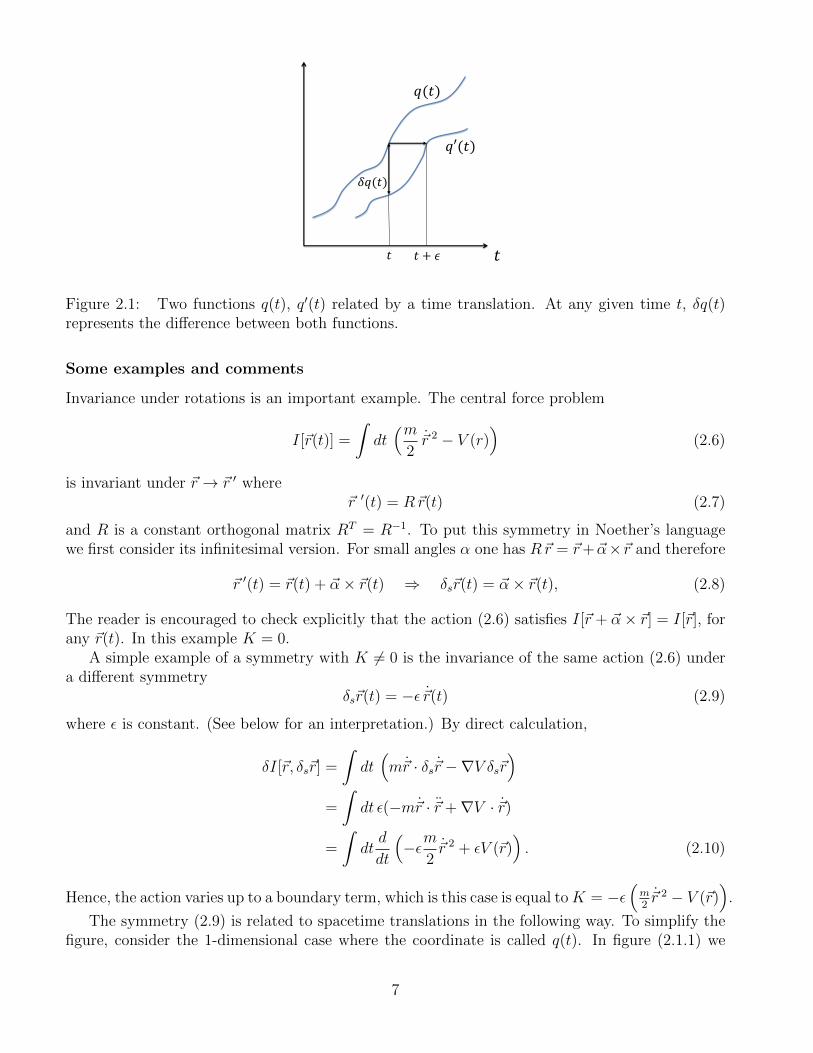
Figure 2.1: Two functions q(t), q′(t) related by a time translation. At any given time t, δq(t)represents the difference between both functions.

Some examples and comments

Invariance under rotations is an important example. The central force problem

I[~r(t)] =

∫dt(m

2~r 2 − V (r)

)(2.6)

is invariant under ~r → ~r ′ where~r ′(t) = R~r(t) (2.7)

and R is a constant orthogonal matrix RT = R−1. To put this symmetry in Noether’s languagewe first consider its infinitesimal version. For small angles α one has R~r = ~r+ ~α×~r and therefore

~r ′(t) = ~r(t) + ~α× ~r(t) ⇒ δs~r(t) = ~α× ~r(t), (2.8)

The reader is encouraged to check explicitly that the action (2.6) satisfies I[~r + ~α× ~r] = I[~r], forany ~r(t). In this example K = 0.

A simple example of a symmetry with K 6= 0 is the invariance of the same action (2.6) undera different symmetry

δs~r(t) = −ε ~r(t) (2.9)

where ε is constant. (See below for an interpretation.) By direct calculation,

δI[~r, δs~r] =

∫dt(m~r · δs~r −∇V δs~r

)=

∫dt ε(−m~r · ~r +∇V · ~r)

=

∫dtd

dt

(−εm

2~r 2 + εV (~r)

). (2.10)

Hence, the action varies up to a boundary term, which is this case is equal toK = −ε(m2~r 2 − V (~r)

).

The symmetry (2.9) is related to spacetime translations in the following way. To simplify thefigure, consider the 1-dimensional case where the coordinate is called q(t). In figure (2.1.1) we

7

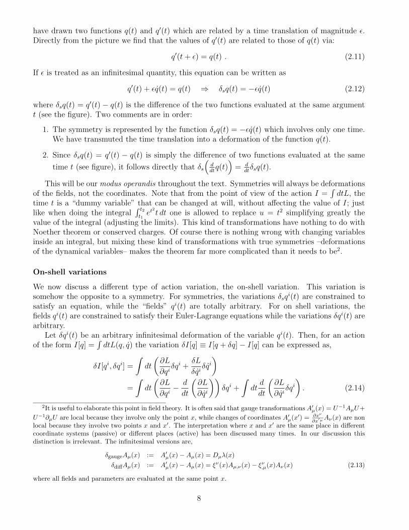
have drawn two functions q(t) and q′(t) which are related by a time translation of magnitude ε.Directly from the picture we find that the values of q′(t) are related to those of q(t) via:

q′(t+ ε) = q(t) . (2.11)

If ε is treated as an infinitesimal quantity, this equation can be written as

q′(t) + εq(t) = q(t) ⇒ δsq(t) = −εq(t) (2.12)

where δsq(t) = q′(t) − q(t) is the difference of the two functions evaluated at the same argumentt (see the figure). Two comments are in order:

1. The symmetry is represented by the function δsq(t) = −εq(t) which involves only one time.We have transmuted the time translation into a deformation of the function q(t).

2. Since δsq(t) = q′(t) − q(t) is simply the difference of two functions evaluated at the same

time t (see figure), it follows directly that δs

(ddtq(t)

)= d

dtδsq(t).

This will be our modus operandis throughout the text. Symmetries will always be deformationsof the fields, not the coordinates. Note that from the point of view of the action I =

∫dtL, the

time t is a “dummy variable” that can be changed at will, without affecting the value of I; justlike when doing the integral

∫ t2t1et

2t dt one is allowed to replace u = t2 simplifying greatly the

value of the integral (adjusting the limits). This kind of transformations have nothing to do withNoether theorem or conserved charges. Of course there is nothing wrong with changing variablesinside an integral, but mixing these kind of transformations with true symmetries –deformationsof the dynamical variables– makes the theorem far more complicated than it needs to be2.

On-shell variations

We now discuss a different type of action variation, the on-shell variation. This variation issomehow the opposite to a symmetry. For symmetries, the variations δsq

i(t) are constrained tosatisfy an equation, while the “fields” qi(t) are totally arbitrary. For on shell variations, thefields qi(t) are constrained to satisfy their Euler-Lagrange equations while the variations δqi(t) arearbitrary.

Let δqi(t) be an arbitrary infinitesimal deformation of the variable qi(t). Then, for an actionof the form I[q] =

∫dtL(q, q) the variation δI[q] ≡ I[q + δq]− I[q] can be expressed as,

δI[qi, δqi] =

∫dt

(∂L

∂qiδqi +

δL

δqiδqi)

=

∫dt

(∂L

∂qi− d

dt

(∂L

∂qi

))δqi +

∫dtd

dt

(∂L

∂qiδqi). (2.14)

2It is useful to elaborate this point in field theory. It is often said that gauge transformations A′µ(x) = U−1AµU+

U−1∂µU are local because they involve only the point x, while changes of coordinates A′µ(x′) = ∂xν

∂x′µAν(x) are nonlocal because they involve two points x and x′. The interpretation where x and x′ are the same place in differentcoordinate systems (passive) or different places (active) has been discussed many times. In our discussion thisdistinction is irrelevant. The infinitesimal versions are,

δgaugeAµ(x) := A′µ(x)−Aµ(x) = Dµλ(x)

δdiffAµ(x) := A′µ(x)−Aµ(x) = ξν(x)Aµ,ν(x)− ξν,µ(x)Aν(x) (2.13)

where all fields and parameters are evaluated at the same point x.

8

where in the second line we have made an integral by parts. This equation contain a powerfulpiece of information. If qi(t) satisfies its Euler-Lagrange equations (2.2), the bulk contributionvanishes and the variation is a total derivative,

δI[qi(t), δqi(t)] ≡ I[qi + δqi]− I[qi] =

∫dtd

dt

(∂L

∂qiδqi). (2.15)

The bar over qi(t) reminds that this variation is evaluated on a solution to the Euler-Lagrangeequations. On the other hand, (2.15) is valid for any δqi(t). This variation depends on theparticular solution chosen qi, and the arbitrary variation δqi.

Noether’s theorem

The combination of a symmetry with an on-shell variation gives rise to Noether theorem. Reca-pitulating, a symmetry is defined by the equation

δI[qi(t), δsqi(t)] =

∫dtdK

dt, (2.16)

and, an on-shell variation is defined by

δI[qi(t), δqi(t)] =

∫dtd

dt

(∂L

∂qiδqi). (2.17)

Both variations are boundary terms but for very different reasons. (2.16) is a boundary termbecause δsq

i satisfies a particular equation, while (2.17) is a boundary term because qi(t) satisfiesa particular equation. On the other hand, qi(t) in (2.16) is totally arbitrary, while δqi(t) in (2.17)is totally arbitrary.

Inserting qi(t) = qi(t) into (2.16) and δqi(t) = δsqi(t) into (2.17) the left hand sides of these

two equations are equal. Subtracting, the left hand sides cancel, and from the right hand sides weobtain the conservation law,

d

dtQ = 0 with Q = K − ∂L

∂qiδsq

i. (2.18)

This is Noether’s First theorem: Given a symmetry δsqi(t), the combination Q showed in (2.18)

is conserved.It is impossible to master Noether theorem without making several examples. The derivation

is very simple but very few students, if any, understands it at first sight. We shall discuss manyapplications of this extraordinary result from 2-dimensional conformal field theory to Maxwell’selectrodynamics.

Our first two examples are the symmetries of the central force potential (2.6) discussed above.The action (2.6) is invariant under rotations with K = 0. The conserved quantity is therefore

Qα = −m~r · δs~r= −m~r · (~α× ~r)

= −~α ·(m~r × ~r

). (2.19)

9

Since ~α is constant and arbitrary we conclude the conservation of angular momentum ~L = m~r× ~r.For the time translation invariance (2.9), we showed in (2.10) that K = −εL. We then concludethat the conserved quantity is,

Qε = −ε(m

2~r 2 − V

)+ εm ~r 2 = εE (2.20)

where E is the total energy.The 4 conserved charges E = m

2r2 + V (r) and ~L = m~r × ~r of the central force problem allows

a simple solution to the equations of motion m~r = −∇V . These are first integrals and the fullsolution is found by doing one integral. We now discuss an example where the full solution isfound purely by looking at symmetries.

2.1.2 The ‘conformal’ particle

A remarkable application of Noether’s theorem is a ‘conformal’ particle. In this example one cansolve the e.o.m. without even having to write them down. Just by looking at the symmetries andmaking use of Noether’s theorem, one can completely integrate the dynamics.

Consider a particle of mass m under the influence of an inverse quadratic potential

I[x] =

∫dt

(1

2mx2 − α

x2

). (2.21)

The equation of motion is

mx =2α

x3. (2.22)

We shall find its full solution by looking at symmetries of the action. We first note that theLagrangian is not explicitly time dependent hence the total energy is conserved:

E =1

2mx2 +

α

x2. (2.23)

This equation provides an algebraic relation between x(t) and x(t). We shall now find a secondequation of this type, which will fix x and x completely.

The second equation follows from the Weyl symmetry of this system:

t→ t′ = λt x→ x′(t′) =√λ x(t). (2.24)

for constant λ. Indeed, under this transformation, dx/dt → d(√λx)/d(λt) = 1√

λdx/dt, and the

action remains invariant,

I →∫λdt

(1

2mx2

λ− α

λx2

)= I . (2.25)

Now, the transformation (2.24) is not useful for Noether’s theorem as it stands. We need toconvert it into an infinitesimal variation acting on x(t) at some time t. Let λ = 1 + ε with ε 1.We expand the transformation of x(t) in (2.24) to first order in ε:

x′ ((1 + ε)t) ≈(

1 +ε

2

)x(t) ⇒ x′(t) + x(t)εt ≈ x(t) +

ε

2x(t) (2.26)

10

from where we extract

δsx(t) = x′(t)− x(t) = −εtx+ε

2x . (2.27)

This transformation acts only on x(t), and is a Noether symmetry of the action:

δI[x] =

∫dt

(1

2mδ(x2)− αδ

(1

x2

))= ε

∫dt

[−m

(1

2x2 + txx

)+ α

x− 2tx

x3

]= ε

∫dtd

dt

[−m

(tx2

2

)+αt

x2

]= ε

∫dtd

dt[−tL] , (2.28)

so the boundary term is K = −tL. Thus, the conserved quantity associated to Weyl symmetry(up to a sign and an ε factor, which are both irrelevant constants)

Q =1

2mxx−

(1

2mtx2 +

αt

x2

). (2.29)

Equations (2.23) and (2.29) are two algebraic equations for x(t) and x(t). From them weobtain x(t) as a function of time, in terms of two integration constants E and Q, as it should fora second order e.o.m. with one degree of freedom. This completely solve the problem. It is left asan exercise to solve these equations, find x(t) and prove that it satisfies (2.22).

Note that, in general, at least one of the conserved charges must be an explicit function oftime, as (2.29), otherwise there would be no dynamics.

It is a good exercise to check explicitly,

dQ

dt=

1

2m(x2 + xx

)− 1

2m(x2 + 2txx

)+ α

(x2 − 2txx

x4

)= (x− 2tx)

[1

2mx− α

x3

]= 0 , (2.30)

due to the e.o.m. (2.22).

2.1.3 Background fields and non-conservation equations

In this paragraph we discuss the role of background fields, and how to deal with them within theframework of Noether’s theorem. Noether’s theorem applied to point particles sheds light intomany aspects of symmetries which sometimes are subtle in field theory. Background fields is anexample.

Consider the following action,

IB[x(t), y(t), z(t)] =

∫ [m2

(x 2 + y 2 + z 2)−B z(t)]dt , (2.31)

where B is a constant. Let us not worry about the origin/relevance of this theory but only aboutits symmetries.

11

The interaction term clearly breaks spherically symmetry. Rotations in the x/y plane remain

a symmetry, but the full O(3) symmetry is broken. Now, let ~B ≡ Bz, we also collect x, y, z intothe vector ~r are rewrite the action as

I ~B[~r(t)] =

∫ [m2~r 2 − ~B · ~r

]dt. (2.32)

This is exactly the same action, simply written in a more elegant way. Both ~r and ~B are vectorswhose components are referred to some set of axes. Applying a rotation of the axes, the scalarproducts ~r · ~B and ~r 2 remain invariant and so the full action is invariant. If R denotes the rotationmatrix we have

IR~B[R~r] = I ~B[~r] (2.33)

Does this “symmetry” imply conservation of angular momentum? No, of course it does not (~L isnot conserved for this system, as can be easily checked from the equations of motion). What iswrong? There is nothing wrong. We just need to be careful with the role of different variablesand transformations.

Equation (2.33) is a mathematical identity and could be called a “symmetry” on its ownright. However, it does not imply a conservation equation because it involves the variation of abackground quantity. Let us apply Noether algorithm to (2.33) to understand what is going on.

We first consider an infinitesimal transformation with angle ~α. The components of ~r and ~B varyas

δs~r = ~α× ~r, δs ~B = ~α× ~B . (2.34)

and one can quickly check that,δI[~r, δs~r] = 0, (2.35)

(that is, K = 0). Of course, this is simply the infinitesimal version of (2.33).We now compute the on-shell variation, i.e. a generic variation of all quantities followed by

use of the e.o.m.,

δI[~r, δs~r] =

∫(−m~r − ~B) · δ~r +

d

dt(m~r · δ~r)− δ ~B · ~r dt

=

∫~α ·(d

dt~L+ ~r × ~B

)dt. (2.36)

and we observe that it is not a total derivative! This is the crucial point. Since the “symmetry”involves the variation of a background quantity, the on-shell variation is not a total derivative.We can proceed with the same logic anyway. Since the symmetry variation is zero, we obtain,

d

dt~L = −~r × ~B, (2.37)

which is the correct torque equation! Noether’s algorithm is very intelligent indeed. It has detectedthat ~L is not conserved, and has given us the rate of change of the would-be-conserved charge.

Dynamical variables (functions of time varied in an action principle) and background quantities(masses, charges or even vectors, tensors but not varied in the action principle) play very different

roles. The vector ~B in (2.32) is an example of a background quantity. Whenever a symmetryinvolves the variation of a background quantity, Noether theorem will not deliver a conservedquantity.

12

From Noether’s point of view, we say that (2.32) is not invariant under rotations becauseI ~B[R~v] 6= I ~B[~r]. The equality (2.33) represents a passive transformation, a transformation whereall vectors remain fixed and only the axes are rotated. But ‘passive transformations’ is not whatNoether symmetries are about. Noether symmetries are those transformations such that, forgiven values of the background quantities, the action is invariant up to a total derivative. Thesesymmetries give rise to conserved quantities.

Some other examples and comments. Consider particle of charge q is in the presence of thefield of a much heavier charge Q. The action is:

I[~r1] =

∫m1

2~r 2

1 −qQ

|~r1 − ~r2|dt . (2.38)

Here ~r1 is a dynamical variable while ~r2, the coordinate of Q, is fixed. This action is not invariantunder translations ~r1 → ~r1 + ~a with constant ~a. As a consequence linear momentum is notconserved. On the other hand ~r1 → ~r1 + ~a together with ~r2 → ~r2 + ~a is a “symmetry”. The timevariation of the momentum can be computed as we did in the example below (exercise!).

One can restore the symmetry by allowing the second charge to move. The action is now,

I[~r1, ~r2] =

∫m1

2~r 2

1 −qQ

|~r1 − ~r2|+m2

2~r 2

2 dt. (2.39)

Although the kinetic pieces are invariant under independent translations ~r1 → ~r1+~a1, ~r2 → ~r2+~a2,the full action is only invariant under the diagonal symmetry with ~a2 = ~a1. As a consequence,only the total linear momentum (center of mass momentum)

~pT = m1~r1 +m2~r2 (2.40)

is conserved (this is easily derivable from the equations of motion).The same applies to angular momentum. The action (2.39) is only invariant under simulta-

neous rotations of both coordinates by the same angle. As a consequence only the total angularmomentum ~L = ~L1 + ~L2 is conserved. If the interaction term was, for example, β

|~r1||~r2| , then the

Lagrangian would remain invariant under independent rotations and therefore ~L1, ~L2 would beconserved independently. But such potential, depending on the relative distances to a third point,does not seem to be physically sound.

Needless to say, all these results are easily derivable from the equations of motion. Our goalhere has been to analyse them in the light of Noether’s theorem. In field theory the equations ofmotion are more complicated and it is often quicker and simpler to apply Noether’s ideas directly.But special care must be observed to get the right results.

2.2 Noether’s theorem in Hamiltonian mechanics: Sym-

metry generators and Lie algebras

Noether’s theorem is applicable to any action, Lagrangian, Hamiltonian, or any other. But theHamiltonian action has extra structure. Consider a general Hamiltonian action,

I[pi, qj] =

∫dt(piq

i −H(p, q)) , (2.41)

13

and its Poisson bracket

[F,G] =∂F

∂qi∂G

∂pi− ∂F

∂pi

∂G

∂qi. (2.42)

The equations of motion are

qi = ∂H∂pi

= [qi, H], (2.43)

pi = −∂H∂qi

= [pi, H]. (2.44)

The time derivative of a function G(p, q, t) (which can be explicitly time dependent) of the canon-ical variables is expressed in terms of Poisson brackets as,

dG(p, q, t)

dt=

∂G

∂qiqi +

∂G

∂pipi +

∂G

∂t

=∂G

∂qi∂H

∂pi− ∂G

∂pi

∂H

∂qi+∂G

∂t

= [G,H] +∂G

∂t. (2.45)

We are interested in conserved charges. Eqn. (2.45) means that a conserved charge Q(p, q, t)satisfies

dQ(p, q, t)

dt= 0 ⇒ [Q,H] +

∂Q

∂t= 0. (2.46)

In many examples the quantity Q has no explicit time dependence, and then (2.46) reduces tohaving zero Poisson bracket with the Hamiltonian3.

We now prove the following important results.

1. Noether’s inverse theorem: If Q is a conserved charge, then the following transformation

δsqi = [qi, εQ] = ε

∂Q

∂pi, δspi = [pi, εQ] = −ε∂Q

∂qi, (2.47)

is a symmetry of the action. This is the inverse theorem because we first assume the existenceof the charge and then build the symmetry.

2. The Lie algebra of symmetries: The set of all conserved charges Qa (a = 1, 2, ...N) satisfiesa closed Lie algebra,

[Qa, Qb] = f cab Qc. (2.48)

The proof of these two statements is extremely simple. We first show that if Q satisfies (2.46)

3 As an example, take a rotational-symmetric system H = 12

(p2x + p2

y

)and consider the quantity Q = xpy−ypx.

Then, the Poisson bracket is simply [H,Q] = −pxpy + pypx = 0 where we never used the e.o.m: it vanishesautomatically.

14

then (2.47) is a symmetry. Varying the action (without using the e.o.m anywhere!)

δI =

∫dt

(δsp q + p

d

dtδsq −

∂H

∂pδsp−

∂H

∂qδsq

)=

∫dt

(−ε∂Q

∂qq +

d

dt(p δsq)− εp

∂Q

∂p+ ε

∂H

∂p

∂Q

∂q− ε∂H

∂q

∂Q

∂p

)=

∫dt

(ε

(−dQdt

+∂Q

∂t+ [Q,H]

)+d

dt(pδsq)

)=

∫dtd

dt

(− εQ+ pδsq

), (2.49)

which is a total derivative, as required for a symmetry. In the last line we have used the assumption(2.46). It is now direct to calculate the on-shell variation and using Noether theorem discover thatthe conserved charge associated to this symmetry is, not surprisingly, exactly Q (exercise!). For amore general form of the theorem, see [11].

Suppose now that we have two conserved charges Q1 and Q2 (both satisfy (2.46)). Then it isa very simple exercise to show explicitly that the commutator [Q1, Q2] is also conserved:

d

dt[Q1, Q2] = [[Q1, Q2], H] +

∂

∂t[Q1, Q2] = 0 (2.50)

Thus [Q1, Q2] is also a conserved charge, and as a consequence generates another symmetry. Now,[Q1, Q2] may be zero, may be a new charge, or it may be proportional to Q1 or Q2. In any case,the conclusion is that a complete set of conserved charges Qa = Q1, Q2, Q3, ... must satisfies a Liealgebra

[Qa, Qb] = f cab Qc. (2.51)

for some structure constants f cab . This algebra is of most importance in the quantum theory.

It is left as an exercise to extend this proof to the case where the charge depends explicitly ontime. The conservation equation then reads,

dQ

dt= [Q,H] +

∂Q

∂t= 0. (2.52)

Given two charges that satisfy (2.52), their Poisson bracket satisfies the same equation. We nowdiscuss the conformal particle, as an explicit example.

2.2.1 The conformal particle in Hamiltonian form

The ‘conformal particle’ of Section 2.1.2 has two conserved charges, with one of them dependingexplicitly on time. Since the system carries only one degree of freedo (two integration constants)these two charges completely solve the equations of motion.

This system in Hamiltonian form has extra structure. See [12] for a detailed treatment, and[13–15] for some applications to the AdS/CFT correspondence. The Hamiltonian action is,

I =

∫ (pq −

(p2

2m+α

q2

))dt (2.53)

15

and three conserved charges (see [12]),

H =p2

2m+α

q2(2.54)

Q = −tH +1

2pq (2.55)

K = t2H + 2tQ− m

2q2 (2.56)

can be found: H,Q,K satisfy (2.52). Of course, given that this theory has only 2 integrationconstants, there exists a relation between the three charges, indeed,

2KH + 2Q2 +mα = 0. (2.57)

The interesting aspect of the Hamiltonian formulation is that H,Q,K satisfy the sl(2,<) algebra,

[Q,H] = H, (2.58)

[Q,K] = −K, (2.59)

[H,K] = 2Q, (2.60)

which is relevant for the AdS2/CFT1 correspondence.

16

2.3 Noether’s theorem in Field theory. Derivation and

examples.

2.3.1 The proof

Just as for particle mechanics, the key to Noether’s theorem is the concept of action symmetries.The simplest field theory example is provided by

I[φ(x)] =1

2

∫d4x ∂µφ∂

µφ. (2.61)

which is clearly invariant under the constant translation φ(x)→ φ(x) +φ0, indeed, I[φ(x) +φ0] =I[φ(x)]. The symmetry now acts on the field φ(x).

The set of symmetries of a field theory action is defined as the set of all infinitesimal functionsδsφ(x) such that, for arbitrary φ(x),

δI[φ, δsφ] ≡ I[φ+ δsφ]− I[φ] =

∫ddx ∂µK

µ ∀ φ (2.62)

for some Kµ. We emphasize:

• Eq. (2.62) is an equation for the function δsφ, not for φ: δsφ is a symmetry provided (2.62)holds for all φ.

• The coordinates play no role. The action is a functional of φ(x) and the coordinates aredummy variables which are ‘summed over’. The definition of symmetry, eq. (2.62), does notinvolve changes in the coordinates in any way. Even for symmetries associated to spacetimetranslations, rotations, etc, they can always be written as some transformation δsφ(x) actingon the field4. We shall discuss this issue in detail in the next paragraph.

The derivation of Noether theorem in field theory follows exactly the same path as in particlemechanics, so we shall be brief.

Field theories in d dimensions are described by actions of the form I[φ(x)] =∫ddx L(φ, ∂µφ)

and the corresponding Euler-Lagrange equations are

E(φ(x)) ≡ ∂µ

(∂L∂φ,µ

)− ∂L∂φ

= 0 . (2.63)

(We will use the notation φ,µ≡ ∂µφ alternatively.) The on-shell variation is computed as

δI[φ, δφ] =

∫d4x

(∂L∂φ

δφ+∂L∂φ,µ

δφ,µ

)=

∫d4x

([∂L∂φ− ∂µ

(∂L∂φ,µ

)]δφ

)+

∫d4x ∂µ

(∂L∂φ,µ

δφ

)=

∫d4x ∂µ

(∂L∂φ,µ

δφ

), (2.64)

4Noether’s symmetries and in general actions symmetries have various formulations some more complicatedthan others. It is possible to formulate symmetries acting directly on the coordinates, and many books choose thispath. We argue that this is not necessary and introduces complications. All symmetries can be understood directlyas a transformation of the field satisfying (2.62). Even the symmetry of general relativity -general covariance- isbest understood as a transformation acting on the metric and not the coordinates (see below).

17

where in the last line we have used that the field φ satisfies its Euler-Lagrange equations.Now, (2.62) is valid for any φ, in particular for φ. Eqn. (2.64) is valid for any δφ, in particular

for δsφ. Thus, inserting φ into (2.62) and δsφ into (2.64) the left hand sides are equal. Substractingboth equations we obtain the conserved current equation

∂µJµ = 0 where Jµ ≡ ∂L

∂φ,µδφ(x)−Kµ (2.65)

This is Noether’s first theorem in field theory.

Before moving to the examples, we show how to build a conserved charge from a conservedcurrent. In a space+time splitting, the continuity equation becomes

∂tJ0 = −∇ · ~J . (2.66)

Integrating both sides of this equation and using the divergence theorem,∫V

d3x ∂tJ0 = −

∫V

d3x ∇ · ~J = −∫∂V

~J · d ~A . (2.67)

If the container V is large enough (and assuming field configurations such that ~J drops to zerofaster than the growth of the surface area) the last integral vanishes, yielding the conserved charge

Q =

∫V

d3x J0(x) withd

dtQ = 0 . (2.68)

Actually, this widespread phrase that “fields fall off sufficiently rapidly at infinity” will turn outto be false in gauge theories. We shall come back to this in Section 4.

2.3.2 Symmetries act on fields: Lie derivatives

We have emphasized that the natural interpretation of a symmetry is as a transformation actingon the field, not the coordinates. The coordinates are dummy variables and in fact one can changethem at will without affecting the value of the integral. This is a basic theorem of calculus. Theaction’s form may change if the coordinates are changed, but not its value. This discussion canbecome a bit subtle and complicated. An easy solution is to realize that for Noether theorem onenever need to change the coordinates. Only the fields transform.

For example, going back to the scalar field action (2.61) one suspects that, besides the sym-metry under φ → φ + φ0, this action is also invariant under constant spacetime translationsxµ → xµ + εµ because there is no explicit dependence on the coordinates. Apparently, then, weface two very different kind of symmetries, some acting on the fields, some acting on the coordi-nates. This is not correct. Within the action, all symmetries can be expressed as transformationsacting on the fields, even symmetries whose origin are variations of the coordinates.

Spacetime translations xµ → x′µ = xµ + εµ are understood as a transformation of the field asfollows: Given φ(x) one builds a new field (‘the translated field’) φ′(x) whose values are

φ′(x) = φ(x− ε)' φ(x)− εµ∂µφ(x). (2.69)

18

where in the second line we retained first order in εµ. The variation of the field which is associatedto a translation of coordinates is then

δφ(x) = −εµ∂µφ(x). (2.70)

This is a local relation involving only the point x. We say that the action (2.61) is invariant underconstant spacetime translations because its variation with respect to (2.70) is,

δI[φ] =

∫d4x ∂µφ ∂

µ(−εν∂νφ)

= −1

2

∫d4x ∂ν(ε

ν∂µφ ∂µφ). (2.71)

a boundary term. No transformation on the coordinates was done. Only a transformation onthe field. Note that a xµ-independent potential U(φ) would not spoil this symmetry becauseδU = U ′(φ)δφ = −U ′εµ∂µφ = −∂µ(εµU), is also a boundary term. This symmetry would be spoiled

if the potential depends explicitly on the coordinates because in that case ∂U(φ,x)∂φ

∂µφ 6= ∂µU(φ, x).

Constant translations are a very special kind of transformation of xµ. One may wonder whetherother important symmetries, e.g., rotations (δ~r = ~ω × ~r), dilatations (δ~r = λ~r), etc5, can also bewritten as a transformation of the field. At the same time, Nature is not composed merely byscalar fields. The general question is, how can a generic transformation δxµ = εµ(x) be interpretedas a variation of the field, if the field is a vector, a tensor, etc?

The solution to this problem is encoded in the transformation laws for tensors

φ′(x′) = φ(x) Scalar (2.72)

V ′µ(x′) =∂x′µ

∂xνV ν(x) Vector (2.73)

A′µ(x′) =∂xν

∂x′µAν(x) (0, 1) tensor (2.74)

g′µν(x′) =

∂xα

∂x′µ∂xβ

∂x′νgαβ(x) (0, 2) tensor (2.75)

...

These equations express the variations of components of various fields when a given transformationof the coordinates is applied. For Noether’s theorem we need the infinitesimal version of theseformulae. We start by calculating the infinitesimal version of the Jacobians appearing in the abovetransformations laws:

x′µ = xµ + ξµ(x) ⇒ ∂x′µ

∂xν= δµν + ∂νξ

µ(x) ,∂xµ

∂x′ν= δµν − ∂νξµ(x′) . (2.76)

With these formulae at hand we go back to the above transformations laws and expand to firstorder case by case.

• Scalar Field: Expanding φ′(x+ ξ) = φ(x) to linear order in ξ we derive

δφ(x) = φ′(x)− φ(x) = −ξν(x)∂νφ(x) . (2.77)

This is same formulae we use before, but not that now ξµ(x) is an arbitrary function of xµ.

5For example, Maxwell’s Lagrangian is (classically) invariant under conformal transformations. We study thiscase in detail below.

19

• Vector field: Expand V ′µ(x′) = ∂x′µ

∂xνV ν(x) to linear order. In this case we need to expand

the left and right hand sides:

V ′µ(x) + ξν∂νVµ(x) = V µ(x) + (∂νξ

µ)V ν(x) , (2.78)

from where we derive

δV µ(x) = V ′µ(x)− V µ(x) = (∂νξµ)V ν − ξν∂νV µ . (2.79)

• (0, 1)−tensor: in the same way as above, the transformation law (2.74) expanded to linearorder at both sides give

A′µ(x) + ξα∂αAµ = Aµ(x)− Aα∂µξα , (2.80)

from where it follows,

δAµ(x) = A′µ(x)− Aµ(x) = −ξα∂αAµ − Aα∂µξα . (2.81)

• (0, 2)−tensor: following the same rules as above, we have at first order in ξ, according to(2.75)

g′µν(x) + ξα∂αgµν(x) =(δαµ − ∂µξα

) (δβν − ∂νξβ

)gαβ(x) (2.82)

= gµν(x)− gµβ(x)∂νξβ − gαν(x)∂µξ

α , (2.83)

from where we deduce

δgµν(x) = g′µν(x)− gµν(x) = −ξα∂αgµν(x)− gµβ(x)∂νξβ − gαν(x)∂µξ

α . (2.84)

The different variations obtained by this procedure are called in the mathematical literatureLie Derivatives. The Lie derivative along a vector ξµ(x) is an operation acting on tensors havinggood transformations laws under coordinate transformations (without involving a connection). Inthis way, the Lie derivative along ξµ(x) of a scalar field, a 1-form and tensor are, respectively,

Lξφ = −ξν∂νφ(x) (2.85)

LξAµ = −ξα∂αAµ − Aα∂µξα (2.86)

Lξgµν = −ξα∂αgµν(x)− gµβ(x)∂νξβ − gαν(x)∂µξ

α . (2.87)

The Lie derivative acting on objects with other index structure can be found in a similar way.

2.3.3 Energy-momentum tensor. Scalars and Maxwell theory

The energy momentum tensor is the Noether current associated to the symmetry under constantspacetime translations xµ → xµ + εµ. The reason that this ‘current’ is really a tensor and not avector field is simple to understand. There is one current associated to time translations t→ t+ε0,another current for space translations in the x direction x→ x+ε1, etc. Altogether, there are foursymmetries and therefore four currents. Of course we don’t split the calculation in this way butcompute the current associated to xµ → xµ + εµ in one step. The current that follows is of courselinear in εµ so it must have the form Jµ = T µνε

ν . The coefficient T µν is the energy-momentum

20

tensor and conservation of Jµ implies ∂µTµν = 0. Put another way, symmetry under spacetime

translations implies the conservation of four independent currents T µν , one for each ν.We compute now the energy-momentum tensor T µν for two specific examples: a scalar field,

and Maxwell’s theory, which is particularly interesting.In relativistic field theories the energy-momentum tensor is often defined as the functional

derivative of the action, Tµν = 1√gδSδgµν

, which is very convenient for many purposes. With a

pedagogical motivation we shall always stick to its definition as the Noether conserved currentassociated to invariance under space-time translations.

Stress tensor for scalar fields

Consider a Lagrangian density for a scalar field L(φ, ∂µφ) which does not depends explicitly onthe coordinates. For example, L = 1

2∂µφ∂

µφ with equations of motion ∇2φ = 06. But the explicitform of the Lagrangian is not relevant here.

If the Lagrangian does not depend on xµ explicitly, then it is invariant under

δφ(x) = −εµ∂µφ(x) , (2.88)

which of course corresponds to the Lie derivative (2.85). Indeed, the variation,

δL =∂L∂φ

δφ+∂L∂φ,ρ

δφ,ρ = −εσ[∂L∂φ

φ,σ +∂L∂φ,ρ

φ,ρσ

]= −∂σ(εσL) (2.89)

is a boundary term. The first equality is the chain rule. In the second equality we simply replacethe symmetry remembering ∂µδφ = δ∂µφ since our variations are the difference of two functions.The crucial step is the third equality which requires that the Lagrangian does not depend explicitlyon xµ7 (and εµ is constant).

The Noether current generated with space-time translations becomes

Jµ = ερ[∂L∂φ,µ

∂ρφ− δµρL]≡ ερT µρ , (2.90)

so the energy-momentum tensor is

T µν(x) =∂L∂φ,µ

∂ρφ− δµρL with ∂µTµρ = 0 . (2.91)

For the free scalar action L = 12∂µφ∂

µφ this yields,

Tµν = ∂µφ∂νφ−1

2ηµν∂αφ∂

αφ. (2.92)

6A typical situation where L depends on xµ is when the field is coupled to external sources J(x), for exampleL = 1

2∂µφ∂µφ+ J(x)φ with equations ∇2φ = J(x).

7It is perhaps worth to give a concrete example. The function f(x(t)) = x(t)2 depends on time only throughx(t). We say that ∂f

∂t =0 while dfdt = f ′(x)x = 2xx. On the other hand, the function g(x(t)) = t x(t)2 depends on t

explicitly and dgdt = x2 + 2txx 6= g′(x)x.

21

Stress tensor for Maxwell’s theory

Let us now study electrodynamics, described by the action

I[Aµ] = −1

4

∫d4x FµνF

µν , Fµν = ∂µAν − ∂νAµ . (2.93)

This theory is invariant under spacetime translations xµ → xµ + εµ with constant εµ, and we cancompute the energy-momentum tensor just as we did for the scalar field. Additionally, Maxwell’stheory is also invariant under gauge transformations δAµ = ∂µλ(x). We shall see now how bothsymmetries can be combined to give a nice energy-momentum tensor which is symmetric andgauge invariant, the Belinfante tensor.

As a motivation for next section we mention that Maxwell’s theory in fact possesses a muchlarger group of Noether symmetry, namely, the conformal group. We display this symmetryexplicitly in the next section and compute the associated conformal currents and charges.

As we see from (2.86), the action of a constant translation on a 1-form Aµ is

δ0Aµ = −εν∂νAµ , (2.94)

where δ0 indicates that this is the variation that we would in principle use. It is left as an exerciseto show that this transformation changes the Maxwell action by a boundary term.

Before continuing with this calculation, we notice that there is an evident problem with thisattempt: the variation (2.94) does not have good properties under gauge transformations (it isnot gauge invariant). One can anticipate that it’s conserved current will not have good propertiesunder gauge transformations either. This problem has been extensively discussed in the literature.We shall jump the discussion and go straight into the solution [16].

Instead of (2.94), consider a transformation that combines a constant spacetime translationtogether with a particular gauge transformation,

δAµ = −εα∂αAµ + ∂µ (εαAα) = Fµαεα , (2.95)

with constant ε. In the literature this is called an ‘improved translation’. It is gauge invariantbecause the derivatives of Aµ appear through only Fµν .

We now compute the variation of the Lagrangian (2.93) under this transformation (usingBianchi’s identity)

δF 2 = 2F µνδFµν = 2F µνεα (∂µFνα − ∂νFµα) = 2F µνεα (∂µFνα + ∂νFαµ)

= −2F µνεα∂αFµν = ∂α(−εαF 2

), (2.96)

which is a boundary term, showing that the improved transformation (2.95) is indeed a symmetry.The variation of the Lagrangian is δL = −1

4∂α (−εαF 2) = ∂α (−εαL) so Kα = −εαL. With this,

the conserved current is

Jµ =∂L∂Aρ,µ

δAρ −Kµ = −F µρεσFρσ + εµL

= εσ [−F µρFρσ + δµσL] = −εσ[F µρFρσ +

1

4δµσF

αβFαβ

](2.97)

and we obtain the electromagnetic energy-momentum tensor,

T µσ = −F µρFσρ +1

4δµσF

αβFαβ . (2.98)

This tensor is gauge invariant (since F is) and has zero trace (associated to the scale invarianceof the classical theory, see below). It is left as an exercise to prove, by direct computation, thatthe energy-momentum tensor (2.98) is indeed a conserved current.

22

2.3.4 Maxwell’s electrodynamics and the conformal group

We have seen that Maxwell’s theory is invariant under constant spacetime translations. They havefour associated currents which form the energy-momentum tensor.

We shall now show that Maxwell’s theory is invariant under a much larger group, the conformalgroup. Constants translations are a small subgroup within the conformal group.

Consider again the transformations xµ → xµ + ξµ(x) where ξµ(x) is now not constant. Asdescribed in (2.86), this transformation acts directly on the field generating a variation,

δ0Aµ(x) = −ξν∂νAµ − ∂µξνAν . (2.99)

Once again this transformation is not gauge invariant but this can be fixed by adding a gaugetransformation just as in (2.95). So we consider the variation (2.99) plus a gauge transformationwith parameter ξνAν

δAµ(x) = −ξν∂νAµ − ∂µξνAν + ∂µ(ξνAν)

= Fµν ξν(x) . (2.100)

We see that the gauge transformation cancels the term with derivatives of ξµ, and at the sametime all derivatives of Aµ appear through Fµν . This variation is called an ‘improved diffeomor-phism’. The same can be done for Yang-Mills fields. (Exercise: prove that the commutator of twotransformations (2.100) with parameters ξµ1 and ξµ2 give a gauge transformation with parameterFµνξ

µ1 ξ

ν2 plus another transformation (2.100) with parameter ξµ = ξν1ξ

µ2,ν − ξν2ξ

µ1,ν).

This improvement of the energy-momentum tensor may seem arbitrary, and even more, prob-lematic: when we add an extra piece to δAµ this should in principle modify the conserved currentand it’s associated charge. This in fact does not occur, because as we shall see in Section 3, gaugesymmetries are not generated by “physical charges” but instead by constraints which vanish on-shell. Thus the “charge” associated to a gauge symmetry is always zero. Therefore adding an extragauge transformation to δAµ does not alter the conserver current, which is the energy-momentumtensor.

Maxwell’s theory is not invariant under (2.100) for arbitrary ξµ(x)8. But it is invariant underall transformations that belong to the conformal group: variations (2.100) such that the vectorsfield ξµ(x) satisfies the particular equation,

ξµ,ν + ξν,µ =1

2ηµνξ

α,α (2.101)

(in 3 + 1 dimensions). Any solution ξµ(x) to this equation provides a Noether symmetry ofelectrodynamics with an associated Noether current and conserved charge. We compute thesequantities below.

Equations (2.101) are called conformal killing equations and can be solved in general. Beforecomputing the currents, we list the solutions to (2.101). To understand the names given to thevarious solutions it is useful to recall that, from the point of view of the coordinates xµ, the vectorsfields ξµ(x) appear in xµ → x′µ = xµ + ξµ(x), or, what is the same, δxµ = ξµ(x).

The vectors ξµ(x) that solve (2.101) are split into the four categories that constitute theconformal group:

8Invariance under a general ξµ(x) is the symmetry of general relativity. When Maxwell’s theory is coupled to adynamical metric it becomes invariant under general diffeomorphisms. The particular form (2.100) is very usefuleven in curved spacetimes.

23

– Constant translations (4 generators). This is the simplest solution to (2.101),

ξµ = ξµ0 . (2.102)

We already know they represent symmetries of Maxwell’s theory.

– Lorentz transformations (6 generators). Slightly less evident, the following vectors

ξµ(x) = εµνxν , εµν = −ενµ (2.103)

also solve (2.101).

– Dilatations (1 generator). A constant rescaling by λ

ξµ(x) = λxµ (2.104)

is also a solution.

– Special conformal transformations (4 generators). The least obvious solution but easilyshown to solve (2.101),

ξµ(x) = 2xνbνxµ − bµxνxν . (2.105)

Let us now prove that the improved transformation (2.100) leaves Maxwell’s lagrangian in-variant (up to a boundary term), if the vector ξµ(x) satisfies (2.101). Our aim is to write thevariation of the Lagrangian as δL = ∂µK

µ + f(ξ), for some function f which depends on ξ butdoes not depend on the field Aµ, because we wish to impose some restriction over the kind oftransformations of coordinates (namely, that they be conformal), but not on the dynamical fields!Starting from L = 1

4F 2, we have

δL = F µν∂µ (ξρFνρ)

= F µνFνρ∂µξρ + F µνξρ∂µFνρ

= F µνF ρν ∂µξρ +

1

2F µνξρ (∂µFνρ + ∂νFρµ)

= −F µνF ρν ∂µξρ −

1

2F µνξρ∂ρFµν

= −F µνF ρν ∂µξρ −

1

4∂ρ (F µνFµν) ξ

ρ

= −1

2F µνF ρ

ν (∂µξρ + ∂ρξµ) +1

4F µνFµν∂ · ξ −

1

4∂ρ(ξρF 2

)= −1

2F µνF ρ

ν

(∂µξρ + ∂ρξµ −

1

2ηµρ∂ · ξ

)− ∂ρ (ξρL) , (2.106)

where we have used the Bianchi identity, and the rest is straightforward calculation. Thus, thetransformation δxµ = ξµ is a symmetry of Maxwell’s action provided that the diffeomorphismsatisfies the conformal Killing equation (2.101).

To derive the conserved current associated to conformal symmetry, we simply repeat Noether’salgorithm as explained above: for transformations satisfying the conformal Killing equation (2.101),the symmetry variation of the Lagrangian is simply (2.106)

δL = −∂ρ (ξρL) , (2.107)

24

while the on-shell variation (2.64) reads:

δosL = ∂ρ

(∂L

∂(∂ρAα)δAα

)= ∂ρ

(F ραξβFαβ

). (2.108)

Equating both derivatives, we find the conserved current associated to conformal symmetry:

Jρ = ξβF ραFαβ +1

4ξρF 2

= ξβ(F ραFαβ +

1

4δρβF

2

)with ∂ρJ

ρ = 0 , (2.109)

where again ξβ is not arbitrary but must belong to any of (2.12)-(2.105). As an aside, it happensthat this classically conserved current does not survive quantisation: the β−functions don’t vanishbecause scaling and special conformal transformations are broken in the quantum theory.

2.3.5 Phase invariance and probability conservation for Schrodinger’sequation

Schrodinger’s equation can be derived from the following field theory Lagrangian

I =

∫dt

∫d3r

(i~ψ∗ ψ − ~2

2m∇ψ∗ · ∇ψ − V (~r)ψ∗ψ

). (2.110)

We find the equations of motion by extremizing the action. Since ψ is complex, ψ and ψ∗ can bethought as independent. Varying with respect to ψ∗ we find

δI =

∫dt

∫d3r

[i~δψ∗ψ − ~2

2m∇δψ∗ · ∇ψ − V δψ∗ψ

]=

∫dt

∫d3r δψ∗

[i~ψ +

~2

2m∇2ψ − V ψ

]+B ,

where B is a boundary term evaluated at spatial infinity where we assume the wave functionvanishes (but again, we will come back to this subtle issue in section 4!). Hence, for arbitraryvariations ψ∗ we find the equations of motion,

i~ψ = − ~2

2m∇2ψ + V ψ = Hψ . (2.111)

It is left as an exercise to find the equations of motion for ψ and show that they are related to the(2.111) by complex conjugation.

Phase invariance and conservation of probability

This action (2.110) is invariant under phase transformations for constant α:

ψ → ψeiα. (2.112)

Let us compute its associated Noether charge. First we need the infinitesimal symmetry transfor-mation,

δψ = iαψ, δψ∗ = −iαψ∗ . (2.113)

25

It is direct to see that the action is strictly invariant under these transformations (i.e. boundaryterm K = 0), so Noether’s charge follows only from the on-shell variation (2.64), by replacing thesymmetry-variation (2.113)

δosI =

∫dt

∫d3r i~

d

dt(ψ∗δψ)

= −α~∫dtd

dt

∫d3r (ψ∗ψ) , (2.114)

where we have assumed again that the field vanishes sufficiently rapidly at infinity so that addi-tional boundary terms vanish. The associated Noether charge is thus

Q =

∫d3r ψ∗ψ , (2.115)

representing the total probability of finding the particle in space. Note finally that the fact that Qis conserved allows to fix it to be equal to one, Q = 1, as one normally does in quantum mechanics.Had

∫ψ∗ψ not been conserved, the definition of probability would be different.

As an exercise, one can carry out Noether’s procedure in the case were the action is definedon a finite volume V with surface S, and one does not assume that the field vanishes there, andshow that in that case the correct conservation equations take the form

∂ρ

∂t+ ~∇ · ~J = 0 , (2.116)

where one must find ρ and ~J as functions of ψ and ψ∗.For some further developments on this subject, see [17].

2.3.6 Two-dimensional conformal field theories: Scalar, Liouville, Diracand bc system

Two dimensional conformal field theories (CFTs) have received huge attention since the seminalwork by Belavin, Polyakov and Zamolodchikov [18]. There exist many families of CFTs classifiedby their central charges. This subject has been treated in great detail in many reviews [19] andalso in textbooks [20], [21].

Our goal in this section will be to derive the energy momentum tensor for the most basicexamples of CFTs, namely, the scalar field, Liouville field, Dirac fields and the bc system, arisingin string theory. The energy momentum tensor is a central object in two dimensional CFTs.However, it if often derived by tricks that don’t apply to all systems. Here we shall follow Noether’stheorem and show that it always gives the right result with no ambiguities. Even for the Liouvillefield, that initially caused some confusion, Noether’s theorem gives the so called improved tensorin one step.

For each example, our strategy is always the same: (i) find the correct variation for the givenproblem; (ii) compute the Noether current (Virasoro charges) (iii) check that they generate thecorrect variations through Poisson brackets; (iii) compute the algebra (Virasoro) and find thevalue of the central charge. In the spirit of providing specific examples, we shall do this forscalars, fermions, the Liouville and the bc system.

2d conformal field theory has infinitely many generators. We emphasize that this does notmean that the symmetry is a gauge symmetry. It only means that there are infinitely manyNoether’s symmetries and infinitely many conserved charges.

26

The applications to string theory are a special case because in the worldsheet action

I[Xµ, hαβ] =

∫ √hhαβ∂αX

µ∂βXνηµν , (2.117)

the field Xµ and the metric hµν are varied. This action is not only conformally invariant butfully diffeomorphism invariant on the worldsheet. The variation over hαβ also makes the energymomentum tensor equal to zero. The conformal generators are zero because they generate asubalgebra of diffeos.

Free scalar field

In most applications of 2d CFT’s, it is most convenient to work in complex coordinates z =et−ix, z = et+ix (for a more detailed treatment, see [20]). Note that in these coordinates, x is theangular variable in the complex plane, and time t relates to the radius of z, such that the infinitepast t = −∞ gets mapped into the origin z = 0, while t =∞ maps to complex infinity.

We start by describing the simplest CFT, namely a scalar field in 2 Euclidean dimensions withaction,

I[φ] =1

4π

∫dzdz ∂φ∂φ , (2.118)

whose the equations of motion are∂∂φ = 0 . (2.119)

The conformal symmetry is evident. Under

z → f(z), z → f(z) , (2.120)

were f(z) is holomorphic (f(z) antiholomorphic) the Jacobian in the volume element gives,

dzdz → |∂f |2dzdz , (2.121)

and the derivatives change in a similar way,

∂φ∂φ→ 1

|∂f |2∂φ∂φ , (2.122)

and therefore the action (2.118) is left unchanged9. In the language of complex analysis, mappingsof the kind (2.120) are called conformal transformations, since they preserve angles locally, orequivalently from (2.121) transform the flat metric into itself multiplied by some overall localfactor. This transformation acted on the coordinates of the manifold. As we have emphasizedalong this review, we now change the logic and express this transformation as a transformationthat acts on the fields only leaving the coordinates untouched. As shown before, this point of viewis important to find the associated conserved charges.

Consider the infinitesimal conformal transformation

z′ = z + ε(z) , z′ = z + ε(z) , (2.123)

9Note that (2.120) produces the following transformation in the 2-dimensional metric,

ds2 = dzdz → |∂f |2dzdz.

27

where ε(z), ε(z) are small arbitrary holomorphic and antiholomorphic functions respectively. Thescalar field φ satisfies, by (2.72):

φ(z, z) = φ′(z′, z′)

= φ′(z + ε, z + ε)

= φ′(z, z) + ε∂φ(z, z) + ε∂φ(z, z) , (2.124)

and from here we derive the transformation,

δφ(z, z) = −ε∂φ(z, z)− ε∂φ(z, z). (2.125)

We check now that the action (2.118) is invariant under the conformal transformation (2.125)without moving the coordinates,

δI = − 1

4π

∫d2z[∂(ε∂φ+ ε∂φ)∂φ+ ∂φ∂(ε∂φ+ ε∂φ)

]= − 1

4π

∫d2z[∂(ε∂φ∂φ

)+ ∂

(ε∂φ∂φ

)], (2.126)

and thus a symmetry. (Observe that the result can be expressed as ∂µKµ.)

Let us compute the Lie algebra of conformal transformations. One can regard z and z asindependent variables and consider one half of the transformation,

δ1φ = −ε1(z)∂φ . (2.127)

Acting with a second transformation,

δ2δ1φ = ε2∂ε1∂φ+ ε2ε1∂2φ (2.128)

we derive,[δ1, δ2]φ = (ε1∂ε2 − ε2∂ε1)∂φ . (2.129)

As expected, the algebra closes : the commutator of two transformations is equal to a new trans-formation with parameter

ε2∂ε1 − ε1∂ε2 . (2.130)

This equation defines the structure constants of this problem. A more explicit form of the structureconstants follows by expanding ε(z) in a Laurent series,

ε(z) =∑n∈Z

εn zn+1 . (2.131)

The transformation of the field (2.125) can be written as,

δφ = −∑

εnzn+1∂φ

=∑

εnLnφ , (2.132)

where we have defined the operator ,

Ln = −zn+1∂ , (2.133)

28

which acts on functions. Let us compute the Poisson bracket of two operators10,

[Ln, Lm]φ = zn+1∂(zm+1∂φ)− zm+1∂(zn+1∂φ)

= (m+ 1)zn+m+1∂φ− (n+ 1)zn+m+1∂φ

= (n−m)Ln+mφ (2.134)

giving a nice representation for the structure constants. This algebra is known as “classicalVirasoro algebra”. In the quantum theory, as well as some classical examples considered below(Liouville theory), (2.134) develops a central term at the right hand side.

We end this paragraph commenting that the other half of the symmetry δφ = −ε∂φ hasassociated operators Ln which satisfy the same algebra (2.134). The two copies of this algebra(one for the holomorphic and another for the antiholomorphic part) are called the “conformalalgebra”.

The action (2.118) possesses an infinite dimensional symmetry, the conformal symmetry andthis symmetry gives rise to conserved charges via Noether’s theorem. Furthermore, in the canon-ical (Hamiltonian) picture, the charges generate the corresponding symmetry transformations viaPoisson brackets, and in the quantum theory, via commutators.

Let us workout the Noether charges associated to the holomorphic conformal transformations.We consider the variation of the action (2.118) under

δsφ = −ε(z)∂φ , (2.135)

with ε(z) holomorphic. Under this transformation, the symmetry-variation is given in (2.126)

δI[φ, δsφ] =1

4π

∫d2z ∂(−ε∂φ∂φ). (2.136)

On the other hand, the on-shell variation of the action is

δI[φ, δφ] =1

4π

∫d2z[∂(δφ∂φ) + ∂(δφ∂φ)

]. (2.137)

Note here that the bar on φ here refers not to complex conjugation but to the classical solutionof the e.o.m.

Inserting (2.135) into the on-shell variation and φ into the symmetry variation The left handsides are equal. Subtracting both equations one derives the conservation law,

∂(ε (∂φ)2 ) = 0 , (2.138)

where we have dropped the bar over the field. Since ε(z) only depends on z, the parameter canbe extracted and we find our conservation law,

∂T = 0, T = −1

2(∂φ)2 , (2.139)

10Note that this procedure is standard in first quantized theories. For example, the wave function in quantummechanics changes under constant translations x → x + a in the form δψ(x) = −a d

dxψ. One then identifies the

translation operator as ddx , which can be expressed in terms of the hermitian momentum operator p = −i ddx , and

have an associated abelian algebra, [p, p] = 0.

29

where the minus sign follows standard conventions. In order to convince ourselves that this doesindeed represent a conservation law, we can repeat the same procedure for the anti-holomorphicside and find, of course,

∂T = 0 , T = −1

2

(∂φ)2

. (2.140)

These two conservations laws can be now written in a more conventional form,

∂(εT ) + ∂(εT ) = ∂µJµ = 0 , (2.141)

where the current has components J z = εT and Jz = εT . However, since ε and ε are arbitrary,this last equation is in fact equivalent to (2.139) and (2.140).

The conservation equation (2.139) gives rise to conserved charges in the standard sense too(and analogously for (2.140)). Recall that given a conserved current Jµ, the integral

∫d3xJ0 is

the conserved charge, which in turn generates the symmetry through the Poisson bracket. Weshall now describe the analogous of this procedure in our complex notation.

Since T (z) is an holomorphic function (as a consequence of the conservation equation) we canexpanded in Laurent modes in the form

T (z) =∑n∈Z

Lnzn+2

, (2.142)

where the Ln are arbitrary coefficients. Soon we will see that these are the conformal generatorsand satisfy the Virasoro algebra. Equation (2.142) can be inverted by multiplying by zm+1 andintegrating on a circle containing the origin at both sides,∮

dz

2πizm+1T (z) =

∑n∈Z

Ln

∮dz

2πi

1

zn−m+1. (2.143)

The right hand side is non-zero only for n = m, so the sum reduces to n = m, and we can solvefor Lm

Lm =

∮dz

2πizm+1T (z). (2.144)

The coefficients Ln are the conserved charges associated to the conformal symmetry. The reasonis the following. By Cauchy’s theorem, the integral in (2.144) does not depend on the radius ofthe circle. Recall now that the time coordinate is equal to t = log |z|. Hence, the independenceon |z| is exactly telling us that the Ln are conserved in time. This is un full analogy with theconservation of

∫Σd3xJ0 whose key property is that the value of the integral does not depend on

which surface Σ is chosen.One last comment regarding the existence of an infinite number of conserved charges. The

conformal symmetry contains a parameter ε(z) which is an arbitrary (analytic) function of z. Thisis quite different from standard global symmetries, like space translations x→ x+ a, involving aconstant parameter a. There is one Noether charge for each parameter in the symmetry. Makinga Laurent series of ε as we did in (2.131), we see that the conformal symmetry does in fact containan infinite number of parameters. As we shall see in the next paragraph, the charge Ln can beseen as the Noether charge associated to the transformation in which only the coefficient of εn isdifferent from zero; in other words, that [φ(z), Ln] = zn+1∂φ.

30

As an exercise, the reader may show that the action (2.118) in also invariant under the affinesymmetry,

δφ = ε(z) , (2.145)

where ε only depends on z. Find the associated conserved charge. What is the algebra of thesecharges?

Light cone quantization: canonical realization of the conformal symmetry

Our last step in the classical description of the conformal symmetry associated to the action(2.118) is to extract the relevant Poisson brackets and check explicitly that the currents T (z) andtheir associated charges Ln do generate these symmetries in the canonical picture.

The Poisson bracket associated to the action

I =1

4π

∫d2z ∂φ∂φ (2.146)

can be extracted by standard methods, via the introduction of a canonical momentum π(x, t).Here we shall follow an alternative route which gives the correct answer in a much quicker fashion,and is better adapted to the corresponding quantum calculation via OPE’s.

The idea is use the coordinate z as time, and derive an equal “time” basic Poisson bracketbetween φ(z) and ∂φ(z). The general method needed is the following.

Consider an action of the form I[w] =∫dt(`a(w)wa−H(w)) where wa denotes collectively all

fields in the theory and `a(w) are some functions of wa. The equations of motion are

σabwb = ∂aH where σab = ∂alb − ∂bla. (2.147)

If σab, called the symplectic matrix, is invertible one can define a Poisson bracket structure asfollows:

[wa, wb] = Jab, Jabσbc = δac , (2.148)

and the equations of motion take the usual form wa = [wa, H]. Furthermore, this Poisson bracketsatisfies the Jacobi identity thanks to the fact that σab is an exact form. See [22, 23] for moredetails and examples of this procedure.

Let us apply this procedure to the scalar field action (2.146) where we interpret z as time. Thefunction `(φ) in this problem is,

`(φ(z)) =1

4π∂φ(z) , (2.149)

and the symplectic matrix σ(z, z′) is,

σ(z, z′) =δ`(φ(z))

δφ(z′)− δ`(φ(z′))

δφ(z)

=1

2π∂′δ(z, z′) . (2.150)

The inverse of σ(z, z′) is

J(z, z′) = 2π1

∂′δ(z, z′) , (2.151)

where 1/∂ is the inverse of the operator ∂. We then find the “equal-time” Poisson bracket

[φ(z, z), φ(z′, z)] = 2π1

∂′δ(z, z′) . (2.152)

31

The presence of 1/∂ in this expression may look intimidating. Fortunately, we shall never need thePoisson bracket of φ with itself, but only with its derivatives. Differentiating (2.152) we deduce,

[φ(z, z), ∂′φ(z′, z)] = 2πδ(z, z′) , (2.153)

which does not have any inverse derivatives, and is the expression we shall need11.As a first check of our newly built Poisson structure, let us check that the Noether charges

associated to conformal transformations have the right properties under it. We have proved thatT = −1/2(∂φ)2 is the conserved charge. An arbitrary conformal transformation with parameterε(z) is generated by

Qε =

∮dz

2πiε(z)T (z) . (2.154)

Now by Noether’s inverse theorem (2.47), we expect Qε to generate the conformal transformationof the field through the commutator. To prove this, we use (2.153) to compute

δφ = i[φ(z, z), Qε]

= −∮

dz′

2πiε(z′)[φ(z, z), ∂φ(z′, z)]∂φ(z′, z)

= −∮

dz′

2πiε(z′) 2πiδ(z′, z)∂φ(z′, z)

= −ε(z) ∂φ , (2.155)

which is, as expected, the correct conformal map of the field, (2.125), for the holomorphic sector.As an immediate consequence, we see that in particular for the Virasoro charges Ln (2.144) (whichare just Qε for ε = zn+1) we have

i[φ(z, z), Ln] = −zn+1 ∂φ . (2.156)

The charge Qε is a linear combination of all conserved charges Ln: by inserting the Laurentexpansions (2.131) and (2.142) for T (z) and ε(z), the integral over z is performed and we find,

Qε =∑n∈Z

εn Ln. (2.157)

As an exercise, recall that the free action is also invariant under affine transformations, δφ =ε(z), whose associated charges are i∂φ =

∑anzn+1 . Show that the inverse transformation is an =∮

dz2πizni∂φ. Show that the Poisson bracket of an gives [an, am] = n δn,m. Find Ln in terms of an.

Compute the Poisson bracket [Ln, am].We are now ready to compute the algebra of generators Ln, now as Poisson brackets of canon-

ical fields. This is totally analogous to computing the algebra of angular momenta in quantummechanics, [Li, Lj] = iεijkLk, that is, the algebra obeyed by the generators of the symmetry. We

11As a footnote we observe that it is incorrect to declare, from (2.146), that 14π∂φ is conjugate to φ. The correct

formula is (2.153).

32

have

i[Ln, Lm] =

∮dz

2πi

∮dz′

2πizn+1z′m+1i

[1

2(∂φ(z))2,

1

2(∂′φ(z′))2

]= −

∮dz

2πi

∮dz′

2πizn+1z′m+1∂φ(z)∂′φ(z′) 2πi ∂′δ(z, z′)

=

∮dz

2πi

∮dz′ zn+1∂′[z′m+1∂′φ(z′)]∂φ(z) δ(z, z′)

=

∮dz

2πizn+1

[(m+ 1)zm(∂φ)2 + zm+1 1

2∂(∂φ)2

]=

∮dz

2πizn+m+1 [(m+ 1)− (n+ 1)]

1

2(∂φ)2

= (n−m)Ln+m . (2.158)

Thus, indeed the conserved charges provide a canonical representation for the conformal algebra(2.134).

Note: The charges Ln do not depend on the contour (they are conserved). The commutatorcan be easily calculated when both contours (for Ln and Lm) are the same, but the result of thecalculation does no depend on that.

Liouville field

Our next example of a classical CFT will be Liouville theory. This is a non-trivial examplebecause, in contrast to the free scalar field, it is a fully interacting theory. For references onLiouville theory we refer, for example, to [24,25].

Liouville theory is defined by the action of a field φ interacting through an exponential poten-tial,

I =1

4π

∫d2z(∂φ∂φ+ Λeφ/γ

). (2.159)

Here Λ and γ are constants. The constant Λ is somehow trivial because it can be redefined byshifting φ. We thus expect this constant not to play any important role. The equation of motionfollowing from (2.159) is,

∂∂φ =Λ

2γeφ/γ. (2.160)

At first sight, Liouville theory is not conformally invariant because the potential is not invariantif the field transforms as a scalar. However, we note that the potential is invariant under a differenttransformations for the field, namely,

eφ(z,z)/γ → eφ′(z′,z′)/γ =

(∂z′

∂z

)−1(∂z′

∂z

)−1

eφ(z,z)/γ. (2.161)

In the language of CFT, this is the transformation for a field of conformal weights (h, h) = (1, 1),but is not primary field12 properly. As we discuss below, it turns out that the kinetic term is also

12A field is called primary with conformal weights h, h if, under any conformal map z → f, z → f it transformsas

φ′(z′, z′) =

(df

dz

)−h(df

dz

)−hφ(z, z). (2.162)

But in (2.161) it is eφ which transforms as a primary field, not φ.

33

invariant under this transformation and hence this is a symmetry of the whole action. This is ofcourse again the conformal symmetry, although it is being represented in a very different way.

Let us first check that the kinetic terms is also invariant. We shall do so by looking at theinfinitesimal transformations. This will also prove to be useful when computing the conservedcharge, and hence the generator of conformal transformations in Liouville theory. We know inadvance that this generator cannot be (∂φ)2 because now the transformations for the field haschanged.

As we did for the non interacting field, for simplicity we shall deal only with half of thetransformations, namely z → z′ = f(z). From (2.161), the transformed field is

φ′(z′) = φ(z)− γ log(∂f) , (2.163)

and its infinitesimal version f(z) = z + ε(z), in terms of δφ = φ′(z)− φ(z), becomes,

δφ = −ε∂φ− γ∂ε . (2.164)

The first piece is clearly the same as that for the scalar field. The full transformation is not thatof a primary field. Our goal now, as usual, is to find the canonical Noether charge that reproducesthis transformation.

We start by checking the invariance of the action under the infinitesimal transformation (2.164).We keep in this calculation all boundary terms.

We start by computing the variation of the potential,

δ(Λeφ/γ

)= Λeφ/γ

−ε∂φ− γ∂εγ

= −∂(Λε eφ/γ

)(2.165)

obtaining a boundary term, as needed. This is of course not a surprise because we already knewthat the potential was invariant under the finite transformation.

Now we want to check that the kinetic part of the action is also invariant under (2.164), whichis not so evident. The transformation (2.164) has two pieces δφ = δ1φ + δ2φ. The first piececorresponds to the original transformation of the free action for the scalar field (2.135), and wealready showed in (2.136) that acting on the kinetic term this transformation gives

δ1

(∂φ∂φ

)= −∂

(ε∂φ∂φ

). (2.166)

On the other hand, the transformation δ2φ is new, and we need to check that it leaves the kineticterm invariant too. Using ∂ε = 0 we find,

δ2

(∂φ∂φ

)= −∂(γ∂ε)∂φ− ∂φ∂(γ∂ε)

= −∂(γφ∂2ε) , (2.167)

which also is a boundary term, as required.We have proved that the Liouville action is conformally invariant, provided the field transforms

as in (2.164). We would like now to extract the associated Noether charge. As we have done allalong this review, to this end we need to compare the boundary terms that we obtained byvarying the action with respect to the symmetry, with the boundary terms that arise in the on-shell variation of the action. The on-shell variation (2.64) evaluated at the symmetry (2.164)gives

δI = − 1

4π

∫d2z[∂((ε∂φ+ γ∂ε) ∂φ

)+ ∂ (∂φ (ε∂φ+ γ∂ε))

], (2.168)

34

while the symmetry-variation is just the recollection of (2.165)-(2.167):

δI = − 1

4π

∫d2z[∂(ε∂φ∂φ

)+ ∂

(γφ∂2ε

)+ ∂

(Λεeφ/γ

)]. (2.169)

Equating (2.168) and (2.169) is the meaning of Noether’s theorem. Simplifying terms and usingthe e.o.m. (2.160), we find

∂((ε∂φ+ γ∂ε)∂φ

)+ ∂ (∂φ(ε∂φ+ γ∂ε)) = ∂

(Λε eφ/γ

)+ ∂

(ε∂φ∂φ

)+ ∂(γφ∂2ε)

∂(ε∂φ∂φ

)+ γ∂

(∂ε∂φ

)+ ∂ (∂φ(ε∂φ+ γ∂ε)) = ∂

(2γε∂∂φ

)+

∂(ε∂φ∂φ

)+ γ∂2ε∂φ

γ∂2ε∂φ+XXXXXγ∂ε∂∂φ+ ∂

(ε(∂φ)2 +XXXXγ∂φ∂ε

)=XXXXX2γ∂ε∂∂φ+ 2γε∂∂2φ+

γ∂2ε∂φ

ε∂(∂φ)2 = 2γε∂∂2φ , (2.170)

from where we read Noether’s conservation law

∂T = 0, T = −1

2(∂φ)2 + γ∂2φ . (2.171)

In the literature [16], this expression for T is called “improved” energy momentum tensor. Addi-tionally, it is direct to show by explicit calculation that ∂T = 0 by use of the e.o.m.

As always, we must now know check that T indeed generates the right conformal transformationof φ via Noether’s inverse theorem (2.47). First of all we note that the Poisson bracket in Liouvilletheory is not different from the free case, because the potential does not introduce any derivativesof the field, so it is still given by (2.153). Furthermore, in total analogy to what was done forthe free scalar in section 2.3.6, the conserved T (z) gives rise to an infinite number of conservedcurrents, with associated conserved charge Qε =

∮dz2πiε(z)T (z) with the correspondent T from

(2.171) for the Liouville action. Then, the symmetry transformation generated by this Noethercharge is

δφ(z) = [φ(z), Qε]

=

∮dz′

2πiε(z′)

[φ(z),−1

2(∂′φ(z′))2 + γ∂

′2φ(z′)

]= −ε∂φ+ γ

∮dz′ε(z′)∂′δ(z, z′)

= −ε∂φ− γ∂ε , (2.172)

which is the correct transformation law for Liouville fields (2.164).The final step is to compute the resulting algebra of the Virasoro generators. Just as for the

free scalar in (2.144), the Virasoro modes are defined as the charges Qε associated specifically tothe ε(z) = zn+1 transformations, namely Ln =

∮dz2πi

zn+1 T (z) so we have

Ln = −∮

dz

2πizn+1 1

2(∂φ)2 + γ

∮dz

2πizn+1 ∂2φ

= L(0)n − γ(n+ 1)

∮dz

2πizn ∂φ (2.173)

where we have called L(0)n the free scalar Virasoro charges, which we already know satisfy the

Virasoro algebra with no central charge (2.158). We also made an integral by parts in the other

35

term, which is useful because ∂φ is primary with conformal dimension 1 with respect to L(0)n . By

direct application of these definitions we first see by differentiating (2.156) that

i[L(0)n , ∂φ] = ∂(zn+1∂φ) . (2.174)

So now we compute the full commutator:

i[Ln, Lm] = i[L(0)n , L(0)

m ] + γ(m+ 1)

∮dz

2πizmi[L(0)

n , ∂φ] + γ(n+ 1)

∮dz

2πizni[∂φ, L(0)

m ]

+ γ2(n+ 1)(m+ 1)

∮dz

2πi

∮dz′

2πiznz′mi[∂φ, ∂′φ′]

= (n−m)L(0)n+m + [(n+ 1)− (m+ 1)]

∮dz

2πizn+m+1

(−γ∂2φ

)(2.175)

+ γ2(n+ 1)(m+ 1)

∮dz

2πi

∮dz′

2πiznz′m∂δ(z, z′)

= (n−m)Ln+m + γ2n(n2 − 1)δn+m,0 .

The central charge is then,c = 12γ2, (2.176)

and depends only on γ, not on Λ, as we anticipated at the beginning. The presence of centralcharges is not an exclusive feature of quantum theories; as this example proves, they can alsoappear in totally classical theories!

Dirac fields in two dimensions

In this subsection we consider another example of a 2d CFT, namely, the massless fermionic fieldin Euclidean spacetime described by the action,

I =1

4π

∫d2x Ψγµ ∂µΨ . (2.177)

Here Ψ is a two dimensional object whose components will be denoted as

Ψ =

(ψψ

). (2.178)

The γµ are the Dirac matrices which satisfy the Euclidean Clifford algebra,

γµ, γν = 2δµν . (2.179)

There are many ways in which to represent the γ′s. A useful two dimensional representation is

γ0 =

(0 11 0

), γ1 =

(0 i−i 0

). (2.180)

Finally, the Dirac conjugated that enters in the action (2.177) is defined as

Ψ = ψ†γ0. (2.181)

36

Just as we did for the scalar field, we shift to complex “light-cone” coordinates z = 12(x+it), z =

12(x− it) implying ∂ = ∂x − i∂t, ∂ = ∂x + i∂t. We now observe that the Lagrangian contains

γ0γ0∂0 + γ0γ1∂1 = ∂0 +

(−i 00 i

)∂1

= −i(∂ 00 −∂

). (2.182)

The action for this free fermion system becomes

I =1

4πi

∫d2z

(ψ∂ψ − ψ∂ψ

), (2.183)

and the problem splits once again in two parts, one holomorphic ψ and one anti-holomorphic.Before carrying on with the analysis we note that our action as it stands does not make much

sense because, naively, ψ∂ψ = 12∂(ψ2). The action is a total derivative and there is no classical

dynamics at all. So what’s going on? The answer is that in order for Dirac’s theory to makesense, even at the classical level we must demand that the fields are not ordinary C numbers butinstead Grassman numbers. These are by definition anticommuting quantities, so that ψ2 = 0 andtherefore ψ∂ψ 6= 1

2∂(ψ2).

The conformal symmetry

Although the action (2.183) is not evidently conformally invariant, in fact it is. The trick isnot to insist that field should transform as scalar under conformal mappings. As we did with thescalar field, we shall treat each sector in the action separately. We then consider only the firstpart of the action (2.183)

I =1

4πi

∫dzdz ψ(z, z)∂ψ(z, z) , (2.184)

which is invariant under the following holomorphic transformation:

z′ = f(z) , z′ = z , ψ′(z′, z′) = [∂f(z)]−1/2ψ(z, z) . (2.185)

(note we have left z invariant). Indeed,∫dz′dz′ ψ′(z′, z′)∂ψ′(z′, z′) =

∫dzdz[∂f(z)][∂f(z)]−1ψ(z, z)∂ψ(z, z)

=

∫dzdz ψ(z, z)∂ψ(z, z) .

The full action (2.183) is invariant under the map (2.185) provided ψ remains unchanged, i.e.transforms as a scalar. ψ and ψ have the following conformal weights:

ψ :

(1

2, 0

), ψ :

(0,

1

2

). (2.186)

The Fermionic Virasoro operator and Canonical structure

We now derive the generator of conformal transformations acting on spinor fields. As usual,we first formulate the symmetry as an operation acting only on the field, not on the coordinates.

37

Expanding (2.185) for the infinitesimal transformation z′ = z + ε(z) to first order (we omit the zdependence which plays no role)

ψ′(z + ε(z)) = (1 + ∂ε(z))−1/2ψ(z)

ψ′(z) + ε(z)∂ψ(z) =

(1− 1

2∂ε(z)

)ψ(z) ,

we derive the transformation rule:

δsψ(z, z) = −ε(z)∂ψ(z, z)− 1

2∂ε(z)ψ(z, z) . (2.187)

The first term in this transformation is the same as of the scalar field, while the second clearlycomes from the extra factor (∂f)−1/2 in the transformation rule.

Compute now the symmetry-variation of the action under the infinitesimal symmetry keepingall boundary terms:

δI[ψ, δsψ] = − 1

4πi

∫d2z

[(ε∂ψ +

1

2∂ε ψ

)∂ψ + ψ∂

(ε∂ψ +

1

2∂ε ψ

)]= − 1

4πi

∫d2z ∂(εψ∂ψ) , (2.188)

which is a boundary term, as expected. Note however that this boundary term is zero on shelland there it will not contribute to the charge.

Compute now the on-shell variation,

δI[ψ, δψ] =1

4πi

∫d2z ∂(ψδψ)

= − 1

4πi

∫d2z ∂

(ψ

(ε∂ψ +

1

2∂ε ψ

))= − 1

4πi

∫d2z ε ∂ (ψ∂ψ) , (2.189)

where we have used that ε is independent of z, and ψ2 = 0 (Grassman variable). We have alsodropped the bar of the field ψ.

The fermionic conserved current associated to conformal symmetry is then,

T = −1

2ψ∂ψ with ∂T = 0 . (2.190)

Our next problem is to find the Poisson bracket associated to this action. We proceed as wedid for the scalar field and treat z as the “time” direction. The function ` is then simply

`(z) =1

4πiψ(z), (2.191)

and the associated “symplectic” form becomes

σ(z, z′) =1

2πiδ(z, z′) . (2.192)

The equal time (i.e. equal z) anticommutator associated to these fermions is then

ψ(z, z), ψ(z′, z) = 2πiδ(z, z′) (2.193)

38

And we observed that it is symmetric as it should for fermionic fields.Finally, let us check that T from (2.190) generates the conformal transformations (2.187). The

conserved charge is again given by Qε =∮

dz2πiε(z)T (z) as in (2.154), and the inverse Noether

theorem gives,

δψ = ψ(z), Qε

=

ψ(z),−

∫dz′

2π

1

2ε(z′)ψ(z′)∂′ψ(z′)

= −1

2

∫dz′

2πε(z′) (ψ(z), ψ(z′) ∂′ψ(z′)− ψ(z′) ψ(z), ∂′ψ(z′))

= −1

2ε(z)∂ψ(z)− 1

2∂(εψ)

= −ε(z)∂ψ(z)− 1

2∂ε ψ . (2.194)

as expected.For the Dirac field, with conformal dimension 1/2 the correct Laurent expansion is

ψ(z) =∞∑

n=−∞

ψnzn+1/2

, (2.195)

and its inverse is

ψn =

∮dz

2πizn−1/2 ψ(z) . (2.196)

Let us compute now the basic anticommutator of the charges ψn,

ψn, ψm =

∮dz

2πizn−1/2

∮dw

2πiwm−1/2ψ(z), ψ(w)

=

∮dz

2πizn−1/2

∮dwwm−1/2δ(z, w)

=

∮dz

2πizn−1/2+m−1/2

= δn+m,0. (2.197)

Note that this is symmetric, as expected. As an exercise, the reader can proceed forward andcompute the Virasoro algebra for the fermionic fields.

The bosonic and fermionic bc systems

Our last example of a CFT in two dimensions is the bc system. These fields appear in the contextof bosonic string theory, in particular when the string is quantised via the path integral method.The b and c fields are the ghosts associated to the gauge fixing when we apply the Faddeev-Popovprocedure. One of the peculiarities of this system is that the fields b, c could be either bosonic orfermionic. As before, the full bc action contains two terms conjugate to one another, so we willfocus only on one pice:

I =1

2πi

∫d2z b∂c . (2.198)

39

It is direct to prove that this action is conformally invariant provided b has conformal weights13

(λ, 0), and c has (1 − λ, 0), which give rise to the respective infinitesimal transformation forholomorphic ε(z),

b′(z′) =

(dz

dz′

)λb(z) ⇒ δb(z) = −ε(z)∂b− λ(∂ε)b (2.199)

c′(z′) =

(dz

dz′

)1−λ

c(z) ⇒ δc(z) = −ε(z)∂c− (1− λ)(∂ε)c (2.200)

What is the Noether current associated to this conformal symmetry? First, we must prove in-finitesimally that (2.199)-(2.200) are indeed a symmetry, and find the boundary term:

δI =1

2πi

∫d2z(δb∂c+ b∂δc

)= − 1

2πi

∫d2z((ε∂b+ λ∂ε b) ∂c+ b∂ (ε∂c+ (1− λ)∂ε c)

)= − 1

2πi

∫d2z((ε∂b+ b∂ε) ∂c+ bε∂∂c

)= − 1

2πi

∫d2z ∂

(εb∂c

), (2.201)

which is indeed a boundary term, but moreover its contribution to the current is proportional to∂c which vanishes on shell. Consider next the generic variation of (2.198) for arbitrary δb, δc:

δI =1

2πi

∫d2z(δb∂c+ b∂δc

)=

1

2πi

∫d2z(δb∂c − ∂b δc+ ∂ (bδc)

)=

1

2πi

∫d2z(eom + ∂ (bδc)

), (2.202)

and evaluating along the e.o.m. and using the particular symmetry (2.199)-(2.200) we get the onshell variation,

δI = − 1

2πi

∫d2z ∂ (bε∂c+ (1− λ)b∂ε c)

= − 1

2πi

∫d2z ∂

(bε∂c+ (1− λ)

(∂ (bεc)− ∂b εc− bε∂c

))= − 1

2πi

∫d2z(ε∂ (λ∂(bc)− ∂bc) + (1− λ)∂∂(bεc)

),

where the last boundary term vanishes on-shell. The Noether current is therefore

T = ∂b c− λ∂(bc). (2.203)

Finally, let’s quickly check that (2.203) generates the correct transformation of the fields. Forsimplicity, let’s assume the fields are bosonic. The Poisson bracket for (2.198) is [c(z), b(z′)] =

13See (2.162)

40

2πiδ(z − z′), and the conserved charge is Qε =∮

dz2πiε(z)T (z), so

δb = [b(z), Qε]

=

∮dz′

2πiε(z′) [b(z), (1− λ)∂′b(z′) c(z′)− λb(z′)∂′c(z′)]

=

∮dz′ε(z′) (−(1− λ)∂′b(z′)δ(z − z′) + λb(z′)∂′δ(z − z′))

= −∂bε− λ∂ε b ,

and similarly for c. One can then show that T does satisfy the Virasoro algebra.

41

Chapter 3

Gauge theories in Hamiltonian form,through examples

3.1 Introduction

Gauge theories play a central role in the development of fundamental theories of physical laws.All three fundamental interactions are described by Lagrangian possessing a gauge invariance: theelectroweak theory, strong interactions and the theory of gravity.

The most well-known gauge theory is Maxwell’s action

I[A] = − 1

16π

∫d4x F µνFµν , (3.1)

having the gauge symmetryδAµ = ∂µΛ(x) . (3.2)

We shall study this theory in detail below. As often happens, though, there are easier ways tounderstand the basics of gauge theories resorting to simple problems in mechanics.

Gauge theories have three important features. First of all the gauge symmetry itself, that is,a transformation containing arbitrary functions of (space-)time. It follows immediately from thegauge symmetry that that there must be relations amongst the various equations of motion of thesystem, and thus not all degrees of freedom in the action will be determined by the e.o.m. Finally,in a Hamiltonian description, a gauge theory has constraints which act as the generators of thecorresponding gauge symmetries.

A theory whose equations of motion do not fully determine the evolution of its variablesmay seem pathological and unphysical at first sight. The great discovery of gauge symmetriesuncovered the concept of equivalent classes of configurations, that is, fields that may differ in theirmathematical presentation but represent the same physical reality: if Aµ is a given solution toMaxwell’s equations, Aµ + ∂µΛ represents the same physical reality, for any Λ(x).

3.2 A quick tour to the classical aspects of gauge theories

Before studying gauge theories in general we shall illustrate the salient points with a “mechanical”model (motivated by electrodynamics). Consider the following action

I[A0(t), ψ(t)] =1

2

∫dt (ψ − A0)2 (3.3)

42

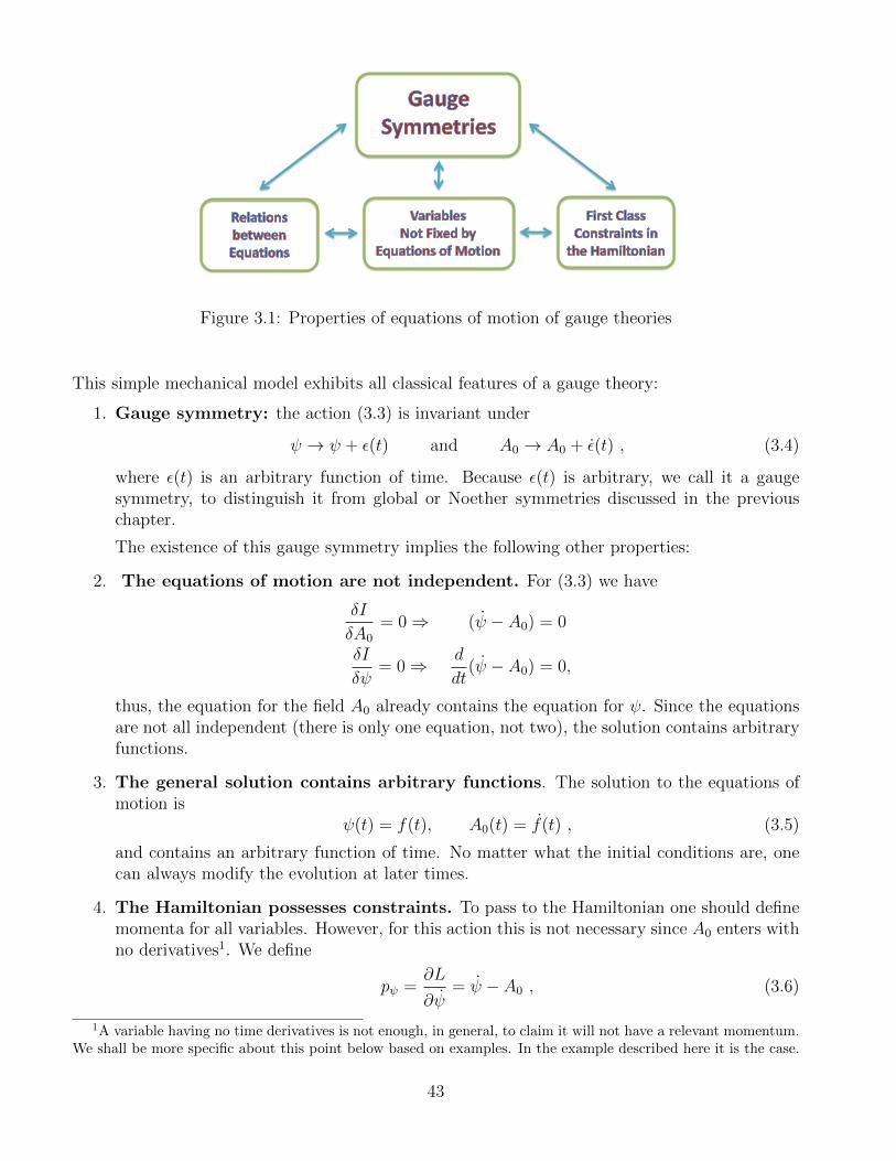
Figure 3.1: Properties of equations of motion of gauge theories

This simple mechanical model exhibits all classical features of a gauge theory:

1. Gauge symmetry: the action (3.3) is invariant under

ψ → ψ + ε(t) and A0 → A0 + ε(t) , (3.4)

where ε(t) is an arbitrary function of time. Because ε(t) is arbitrary, we call it a gaugesymmetry, to distinguish it from global or Noether symmetries discussed in the previouschapter.

The existence of this gauge symmetry implies the following other properties:

2. The equations of motion are not independent. For (3.3) we have

δI

δA0

= 0⇒ (ψ − A0) = 0

δI

δψ= 0⇒ d

dt(ψ − A0) = 0,

thus, the equation for the field A0 already contains the equation for ψ. Since the equationsare not all independent (there is only one equation, not two), the solution contains arbitraryfunctions.

3. The general solution contains arbitrary functions. The solution to the equations ofmotion is

ψ(t) = f(t), A0(t) = f(t) , (3.5)

and contains an arbitrary function of time. No matter what the initial conditions are, onecan always modify the evolution at later times.

4. The Hamiltonian possesses constraints. To pass to the Hamiltonian one should definemomenta for all variables. However, for this action this is not necessary since A0 enters withno derivatives1. We define

pψ =∂L

∂ψ= ψ − A0 , (3.6)

1A variable having no time derivatives is not enough, in general, to claim it will not have a relevant momentum.We shall be more specific about this point below based on examples. In the example described here it is the case.

43

and the Hamiltonian is

H(pψ, ψ, A0) = pψψ − L (3.7)

=1

2p2ψ + A0pψ . (3.8)

The corresponding Hamiltonian action is

I[pψ, ψ, A0] =

∫ (pψψ −

1

2p2ψ − A0pψ

)dt (3.9)

The equations that follow from this action varying A0, ψ and pφ are totally equivalent tothose following from (3.3). We see that A0 appears as a Lagrange multiplier,

δI

δA0

= pψ = 0 , (3.10)

and we find our first example of a constraint, an equation involving no time derivatives. Thetwo remaining e.o.m. are

δI

δp= ψ − pψ − A0 = 0 (3.11)

δI

δψ= −pψ = 0 , (3.12)

where again one equation (3.12) is already contained in another one (3.10), so clearly fromthe Hamiltonian point of view we again have less equations than unknowns.

We shall end the description of this model by briefly mentioning the issue of gauge fixing. Agauge theory has more undetermined functions than equations. To make sense of the evolutionone could either look for gauge invariant functions, like electric and magnetic fields in electromag-netism, or fix the gauge by imposing one condition per gauge freedom. Fixing the gauge is notalways the best procedure because often is breaks locality. The powerful BRTS methods has beendeveloped to this end.

Here we shall only make some remarks on how one would fix the gauge in this model, stressinga subtle point. In this example we have one gauge symmetry so we can impose one condition. Isit the same to impose A0 = 0 or ψ = 0 as gauge condition? It is not. The reason is that, as wesaw before, the equation of motion for ψ is contained in the equation for A0, but not the otherway around. This means that one can dispose of ψ(t) and no information will be lost because itsequation is already there. But one cannot dispose of A0. To see this more explicitly, if we fix thegauge ψ = 0 in the action (3.3) we have

Iψ=0[A(t)] =

∫dt A2

0eom→ A0(t) = 0 , (3.13)

The general formalism to deal with Hamiltonian version of gauge theories is Dirac’s constraint analysis. Whenpossible we shall avoid the general analysis and derive the right results in a more economical way. It is left asan exercise to prove that defining momenta for both variables yields no new information, but makes the analysislonger.

44

which uniquely fixes A0(t), and shows that the pure-gauge action (3.3) in fact has no degrees offreedom at all. However, consider now what happens if instead we fix A0(t) = 0 (incorrect!) asgauge condition. The action becomes

IA0=0[ψ(t)] =

∫dt ψ2 eom→ ψ = 0 , (3.14)

which represents a free field ψ that does carry one degree of freedom! Setting A0 = 0 insidethe action is incorrect because, as we discussed above, the equations of motion for A0 are notcontained in those of ψ.

The model we have just described captures all the characteristic features of a gauge theory.In the following section we shall present the general Hamiltonian structure of gauge theories,and then proceed to show how the most important cases (Maxwell’s theory, Yang-Mills theory,and General Relativity) all fall into this classification. We shall also consider 2+1 Chern-Simonstheories basically because they are extremely simple and of great pedagogical value.

For other applications of Noether’s second theorem, see [26,27].

3.3 General structure of gauge theories in Hamiltonian

form

There are many actions possessing a gauge symmetry; from electrodynamics to general relativity,from a relativistic particle to the string worldsheet. One of the nice features of the Hamiltonianformulation is that it provides a unified framework for all of them. In this way, many features canbe studied in a general setting valid for all examples.

In most cases the Hamiltonian is derived from the Lagrangian. In the presence of gaugeinvariance this process, devised by Dirac long ago, can be long and painful. The final result ishowever neat and clear.

In this section we shall present gauge theories in the reverse order. We start with the Hamilto-nian action from scratch describing its properties and the role of the different ingredients. After-wards, we present the classic examples starting as usual from the Lagrangian and going throughthe Legendre transformation into the Hamiltonian.

All2 gauge theory actions, when written in Hamiltonian form, have the following generic form

I[pi, qi, λa] =

∫dt(piq

i −H0(pi, qi) + λaφa(p, q)

)(3.15)

This will be our “paradigm” of a Hamiltonian gauge theory. Here pi, qi and λa are independent

fields varied in the action. The total (or “extended”) Hamiltonian H = H0− λaφa is decomposedin two terms: H0 denotes that part of the Hamiltonian (if any) that is not a constraint, while λaφaincludes the contributions from the constraints φa. Note that this action contains no derivatives

2Here we mean most well-known and useful examples: Maxwell’s theory, Yang-Mills theories, General Relativity,and many others.

45

of the λ’s. Varying with respect to pi, qj and λa, the equations of motion are

qi =∂H0

∂pi− λa∂φa

∂pi, (3.16)

pi = −∂H0

∂qi+ λa

∂φa∂qi

, (3.17)

φa(p, q) = 0. (3.18)

This system of equations is very interesting. All characteristic properties of a gauge theory arecontained in the presence of the Lagrange multipliers λa(t) and constraints the φa(p, q).

The first two equations determine the evolution of p, q given initial conditions p0, q0. Onenotices, however, that the initial conditions cannot be totally arbitrary because they must satisfythe constraints (3.18); also to actually integrate (3.16) and (3.17) one needs the functions λa(t).Two questions immediately come to one’s mind (i) How do we choose the functions λa(t)? (ii)Given initial conditions that do satisfy the constraints (3.18), is it guaranteed that the timeevolution dictated by (3.16) and (3.17) will preserve the constraint (3.18)?

Both questions can be answered at once by computing the time derivative of the constraints.Using (3.16) and (3.17) to express qi and pi in terms of derivatives of H0 and the constraints wefind,

d

dtφa(p, q) = [φa, H0]− [φa, φb]λ

b. (3.19)

Now, the constraints (3.18) must hold for all times, this means that the evolution will be consistentprovided φa vanishes at all times, that is,

[φa, H0]− [φa, φb]λb ≈ 0. (3.20)

The symbol ≈ 0 (“weakly zero”) means that we do not require φa to be strictly zero, it is enoughif it vanishes when φa is zero. Equation (3.20) is a consistency condition for the time evolution.Calling Cab = [φa, φb], the following situations may occur:

1. Non-gauge theories: If the matrix Cab is invertible, then (3.20) fixes completely thefunctions λa(t),

λa(t) = Cab [φb, H0] . (3.21)

In this case, the role of the functions λa(t) is to preserve (3.18). The system (3.16)-(3.18)is then well understood: one gives initial conditions satisfying (3.18); the functions λa aredetermined by (3.21), ensuring that (3.18) is satisfied at all subsequent times. In Dirac’slanguage this is a theory with second class constraints. The first applications of Lagrangemultipliers fall in this class of systems well before Dirac’s theory!

But we are interested in gauge theories. These arise in the opposite case.

2. Gauge theories: If the matrix Cab is zero, or more generally, if this matrix is weakly zeroCab ≈ 0, i.e. zero on the surface φa = 0, then (3.20) imposes no restrictions on the functionsλa(t) (again on the surface φa = 0) which therefore remain undetermined by the e.o.m. Wesee the first signal of a gauge theory: the dynamical evolution contains arbitrary functionsof time. Now, if [φa, φb] = 0, then (3.20) imply also that [φa, H0] = 0. A set of constraintsare defined as first class if they satisfy

[φa, H0] = C ba φb , [φa, φb] = C c

ab φc , (3.22)

46

which are both weakly zero.

A remarkably general result is now the following: if the Hamiltonian and the constraintssatisfy (3.22), then the action (3.15) is invariant under the following transformations,

δqi = [qi, φa]εa(t) (3.23)

δpi = [pi, φa]εa(t) (3.24)

δλc = εc + εa(t)C ca − λaεb(t)C c

ab , (3.25)

where εa(t) are arbitrary functions of time. These transformations are the gauge symmetryof the system. We have thus inverted the logic. All actions of the form (3.15) where theconstraints and Hamiltonian satisfy (3.22) have a gauge symmetry. (This is the analogue ofNoether’s inverse theorem discussed above; for an extension, see [11]). We prove this resultbelow. Before we mention the mixed case:

3. Mixed case. Of course one may find mixed cases where some constraints are first classand some other are second class. See [28, 29] for a non-trivial example. One could also findsystems where conditions (3.20) lead to new constraints, called secondary constraints. Fromnow on we shall focus on gauge theories, that is, theories for which (3.22) holds.

Proof of gauge invariance: Assuming (3.22) holds we prove invariance of the action (3.15)under (3.24)-(3.25). The variations of the canonical variables are

δqi = εa∂φa∂pi

, δpi = −εa∂φa∂qi

, (3.26)

then (B stands for boundary terms that we drop)

δI = δ

∫dt(piq

i −H0 − λaφa)

=

∫dt[− εa∂φa

∂qiqi − piεa∂φa

∂pi+B − ∂H0

∂qiεa∂φa∂pi

+∂H0

∂piεa∂φa∂qi

+

− δλaφa − λa(∂φa∂qj

εb∂φb∂pj− ∂φa

∂pjεb∂φb∂qj

)]=

∫dt

[−εa d

dtφa − εa[H0, φa]− δλaφa − λaεb[φa, φb] +B

]. (3.27)

If φa are all first class constraints they satisfy (3.22), the variation becomes

δI =

∫dt[εaφa + εaC b

a φb − δλaφa − λaεbC cab φc

]+B

=

∫dt(εc + εaC c

a − δλc − λaεbC cab

)φc +B

= B , (3.28)

where we have used (3.25) (and have redefined B several times).Comments:

• No charge

47

The gauge symmetry is a symmetry of the action and one could in principle compute itsNoether charge. It is left as a exercise to prove that the result is φa. That is the chargeexists but has a zero value on all solutions. See also [11].

• Degrees of freedom: one must note the crucial difference in the number of d.o.f. of a non-gauge theory vs that of a gauge theory:

1. In a non-gauge theory I =∫dt (piq

i −H0), with i = 1, . . . , N , the full solution of thedynamics

qi =∂H0

∂pi, pi = −∂H0

∂qi, (3.29)

requires 2N integration constants, so there there are simply 12× 2N physical d.o.f.

2. In contrast, a gauge theory I =∫dt (piq

i −H0 − λaφa) containing the same 2N canoni-cal variables has the additional constraints φa with, say, a = 1, . . . , g. The equations are(3.16),(3.17),(3.18). In principle we need 2N intergartion constants. However, φa = 0subtracts g of them. There are also g gauge symmetries which imply that the pi and qiare not by themselves physically meaningful, but rather there exists some combinationsof them that are. This reduces another g constants as physically meaningful. The totalnumber of d.o.f. is 1

2(2N − 2g).

• In gauge theories, the time evolution (3.16),(3.17),(3.18) of the canonical variables is theusual one, q = ∂pH0 and p = −∂qH0, plus an additional term, λa∂pφa and λa∂qφa which is agauge transformation (3.23)-(3.24) with the gauge parameter being the Lagrange multipliers.

3.4 Executive review of examples

Many very important physical theories lie in this category. In this section we will consider theexamples listed below, for which we exhibit their Hamiltonian action highlighting the constraintsin blue:

1. The free spinless relativistic particle - in section 3.5.1 we will show

I[x, λ] =

∫dτ[pµx

µ − λ(p2 +m2

)], (3.30)

which, when written in this gauge invariant form, has H0 = 0.

2. Free Electrodynamics - in section 3.5.2 we’ll write Maxwell’s action as:

I[Ai, Ei, A0] =

∫d4x

[EiA

i −(

1

2E2i +

1

4F 2ij

)+ A0∂iE

i

]. (3.31)

3. Yang-Mills - although we won’t review it here, it’s the generalisation of (3.31)

I[Ai, Ei, A0] =

∫d4x

[EiaA

ai −

(1

2Ea2i +

1

4F a2ij

)+ Aa0DiE

ai

]. (3.32)

48

4. General Relativity: in section 3.5.3, we study the Einstein-Hilbert action in its ADM form,

I[gij,Πij, N,Ni] =

∫d4x

[Πij gij −NH−NiHi

], (3.33)

which possesses four constraints. Here also, the Hamiltonian is zero (it’s a constraint).

5. Chern-Simons theory: in section 3.5.4 we’ll consider 3d gravity through

I[A] =k

2π

∫d3x εijηab

(−Aai Abj + Aa0F

bij

). (3.34)

For each one of these examples, we’ll follow the same systematic procedure:

• Introduce the Lagrangian form,

• Derive its Hamiltonian action,

• Show how the constraints generate the gauge symmetry.

We emphasise that all gauge theories can be understood within the general structure (3.15). Thisprovides not only a greater conceptual clarity about the common features of all gauge theories,but also serves when dealing with more complicated systems.

3.5 Examples in detail

In this section we show in detail how to go from the Lagrangian actions into the general form(3.15) for the examples just displayed. For some recent applications in connection to the Wardidentities, see [30].

3.5.1 The relativistic point particle

The action for a spinless relativistic point particle parametrised as xµ(τ) is

I = −m∫ds = −m

∫dτ

√−dx

µ

dτ

dxν

dτηµν , (3.35)

where xµ = dxµ

dτ. Here τ stands for any parameter describing the curve (not necessarily proper

time). As is well known and clear from (3.35), the action is invariant under the unphysicalreparametrisation:

τ ′ = τ ′(τ) , x′µ(τ ′) = xµ(τ) . (3.36)

As usual, one is also interested in expressing this symmetry as an infinitesimal transformation ofxµ (the “field”) rather than of the parameter τ (the “coordinate”). Taking τ ′ = τ + ε(τ), (3.36)implies

x′µ(τ + ε) = xµ(τ) ⇒ δxµ(τ) = −ε(τ)xµ , (3.37)

49

and one must now show explicitly that this variation is a symmetry of the action (3.35):

δI = −m∫dτ−xµδxµ(−x2)1/2

= −m∫dτ

d

dτ

(ε(τ)

(−x2

)1/2), (3.38)

and thus the boundary term is K = −mε(τ) (−x2)1/2

= ε(τ)L. If one keeps going and tries to findthe associated Noether’s charge, this will be zero (“gauge” conserved quantities are always zero!).

What about the Hamiltonian version? In principle, one would wish to define H from thisaction and leave the Hamiltonian action in our favorite form I =

∫px−H0 +λφ as in (3.15). But

after writing down the canonical momentum,

pν =mxν√−xµxµ

, (3.39)

one is incapable of solving xµ in terms of pµ. This is because although (3.39) seems to represent 4independent equations, they are only 3, since there is a constraint: contracting (3.39) with itself,

φ ≡ pνpν +m2 = 0 , (3.40)

is satisfied without the e.o.m. This issue is taken as the starting point of Dirac’s method of con-straints, which we will not cover in these notes. Now, instead of defining the Hamiltonian versionof the action (3.35), we review the method of Polyakov, which does provide a straightforwardHamiltonian formulation.

The Polyakov action There is another way of writing the relativistic action, by introducingan auxiliary variable, the einbein e(τ) which is treated as a dynamical field, and by defining thePolyakov action

IP [xµ(τ), e(τ)] =1

2

∫ (1

exµxµ − e m2

)dτ . (3.41)

This action exhibits precisely the property highlighted in (3.15): the Lagrangian contains noderivatives of the einbein, so we can use its equation of motion

∂L

∂e= 0 ⇒ e(xµ) =

1

m

√−x2 , (3.42)

and replace it into the Polyakov action (3.41), which gives back the relativistic action (3.35).Therefore the Polyakov action is classically completely equivalent to the original relativistic action(3.35), but with a fundamental advantage: it is quadratic in the field x, something which is of hightechnical importance in order to quantize the theory. Since they are equivalent, the Polyakov actionshould also be invariant under reparametrization, but now we must determine the transformationlaw for the additional auxiliary field. In addition to (3.36), the transformation law

e′(τ ′) = e(τ)dτ

dτ ′, (3.43)

50

is easily seen to render the action invariant. The infinitesimal version of this as a transformationof the field instead of the coordinates is

e′(τ + ε) = e(1− ε) ⇒ δe(τ) = − d

dτ(ε(τ)e) , (3.44)

so the complete symmetry transformation of the fields under reparametrisation is

δxµ(τ) = −ε(τ)xµ , δe(τ) = − d

dτ(ε(τ)e) , (3.45)

and this is indeed a symmetry, for the variation of (3.41) under this transformation is

δIP =1

2

∫dτ

(2exµδxµ − x2δe

e2−m2δe

)(3.46)

= −1

2

∫dτ

d

dτ

(ε

(x2

e−m2e

)), (3.47)

that is, a boundary term K = −12ε(τ)

(x2

e−m2e

)= −ε(τ)L.

The Hamiltonian for the Polyakov action is easily found to be

H(pµ, xµ, e) =

1

2e(pµp

µ +m2), (3.48)

and therefore the Hamiltonian Polyakov action∫pq −H reads

IP [p, x, e] =

∫dτ

[pµx

µ − 1

2e(pµp

µ +m2)]

(3.49)

This has precisely the form (3.15) for a Hamiltonian action with one gauge symmetry, “free”Hamiltonian H0 = 0, the einbein e playing the role of the Lagrange multiplier, and φ = 1

2(p2 +m2)

is the constraint. The fact that H0 = 0 here is due to the gauge invariance: the Hamiltonian isnot conjugate to any physical time, because we are using the arbitrary parameter τ to describethe evolution.

Finally, in order to close the logical circle, let’s check that indeed the constraint φ generates thegauge transformation (3.37) through Poisson brackets. This must be so because H0 = 0 and allthe Cab = [φa, φb] = 0 are zero in this example because there’s a single constraint so it’s triviallyfirst class; using (3.23)-(3.25),

δxµ = [xµ, ε(τ)1

2(p2 +m2)] = ε(τ)pµ

δpµ = [pµ, ε(τ)1

2(p2 +m2)] = 0

δe = ε(τ) ,

so the variation of the action is indeed a boundary term:

δI =

∫dτ

[pµδx

µ − 1

2δe(p2 +m2

)]=

∫dτ

d

dτ

[1

2ε(τ)

(p2 −m2

)]. (3.50)

51

3.5.2 Maxwell theory

To define a Hamiltonian action, we start by rewriting the electromagnetic Lagrangian by separatinginto its space+time components in order to define a canonical structure:

IEM = −1

4

∫d4x F µνFµν

=

∫d4x

[−1

2F 0iF0i −

1

4F ijFij

]=

∫d4x

[1

2(Ai − ∂iA0)(Ai − ∂iA0)− 1

4FijF

ij

]=

∫d4x

(1

2AiA

i − Ai∂iA0 +1

2∂iA0∂

iA0 −1

4FijF

ij

). (3.51)

As before, we define canonical momenta only for those variables that appear with temporalderivatives in the action; in this case, Ai,

πi ≡∂L∂Ai

= Ai − ∂iA0 ⇒ Ai = πi + ∂iA0 . (3.52)

Note from this that πi is the electrical field: ~π = ~E. The Hamiltonian is

H(p,A) = πiAi − L

= πi(πi + ∂iA0)−

[1

2(πi + ∂iA0)(πi + ∂iA0)− (πi + ∂iA0)∂iA0 +

1

2∂iA0∂

iA0 −1

4FijF

ij

]=

1

2πiπ

i +1

4FijF

ij − A0∂iπi , (3.53)

where we have integrated by parts in the last line and dropped the boundary term (we postponethe important discussion of boundary terms for section 4!).

Thus, the Hamiltonian action∫pq −H for electromagnetism is

IEM [Ai, πi, A0] =

∫d4x

[πiA

i −(

1

2πiπ

i +1

4FijF

ij

)+ A0∂iπ

i

](3.54)

which again has precisely the general form (3.15) I =∫pq − H0 + λaφa , where H0 is the “dy-

namical” Hamiltonian (the energy) and A0 the Lagrange multiplier

H0 =1

2πiπ

i +1

4FijF

ij =1

2

(~E2 + ~B2

), λ = A0 , (3.55)

while the only constraint is Gauss’ law:

φ = ∂iπi = ∇ · ~E = 0 . (3.56)

With regards to Hamilton’s equations of motion

πi = − ∂H∂Ai

, Ai =∂H

∂πi, φ = 0 , (3.57)

52

one is confronted with the same issues discussed after (3.18), namely that we must guarantee thatthe e.o.m. will preserve the vanishing of the constraint, provided we choose some initial conditionsthat do. As we mentioned there, all we need to do is to demand that dφ

dt= [φ,H] = 0. Since we

are now in a field theory, we must actually compute [φ(x), H(x′)] where x and x′ are two distinctspace-time points:

[φ(x), H(x′)] =

[∂iπ

i(x),1

2

(πiπ

i(x′) + FijFij(x′)− 1

2A0∂iπ

i(x′)

)]. (3.58)

Here we must use the field theory symplectic structure:

[πi(x), πj(x′)] = 0 , [Ai(x), Aj(x

′)] = 0 , [Ai(x), πj(x′)] = δijδ

3(x− x′) , (3.59)

which yields

dφ

dt= [φ(x), H(x′)]

= 2∂k∂′i [πk(x), Aj(x

′)]F ij(x′)

= −2(∂k∂

′iδ

3(x− x′))F ik(x′) = 0 , (3.60)

due to symmetry-antisymmetry in (i, k). The constraint φ is therefore a conserved quantity alongthe classical evolution of the system, and must generate the gauge symmetry through the field-theoretic version of (3.23)-(3.25), which is as follows. In the Poisson bracket, instead of consideringsimply the constraint function φ(x) = ∂iπ

i(x) we must take a functional Φ[Λ(x)] depending onsome arbitrary “weight” test function Λ(x) which will act as the gauge function:

Φ[Λ(x)] =

∫d3x Λ(x)∂iπ

i(x) , (3.61)

where we only integrate in space and not in time because we wish Φ to remain a function of time,so that we can compute an ‘equal time’ commutation relation with something else. The gaugetransformations, analogous to (3.23)-(3.24), are defined as the bracket with the functional Φ:

δAi(x) = [Ai(x, t),Φ[Λ]]

=

∫d3x′Λ(x′, t)∂′j

[Ai(x, t), π

j(x′, t)]

=

∫d3x′Λ(x′, t)δji∂

′jδ

(3)(x− x′)

= −∂iΛ(x, t) , (3.62)

which is precisely the form of the spatial gauge transformation of electrodynamics! On the otherhand, the transformations of the momenta vanish:

δπi(x, t) = [πi,Φ[Λ]] =

∫d3x′Λ(x′, t)

[πi, ∂jπ

j]

= 0 , (3.63)

which must be so - the momentum is the electric field, πi = Ei, which must better be gauge invari-ant. Finally, the transformation law for the Lagrange multiplier A0, just as in (3.28), is deduced

53

from the requirement that, under the gauge transformations (3.62) and (3.63), the variation ofthe action must be only in a boundary term (i.e. the transformations must be a symmetry)

δI =

∫d4x

[πiδA

i + δA0 φ]

=

∫d4x

[−πi∂i∂0Λ + δA0 ∂iπ

i]

=

∫d4x

[∂i(−πi∂0Λ

)+ ∂iπ

i ∂0Λ + δA0 ∂iπi]

=

∫d4x

[∂µK

µ + ∂iπi (δA0 + ∂0Λ)

], (3.64)

with Kµ = (0,−πi∂0Λ), and we have used δπi = 0, δφ = 0, δH0 = 0 since they are all gaugeinvariants. Thus we need δA0 = −∂0Λ in order for δI to be a boundary term3. Thus we concludethat the gauge transformation of the field Aµ generated by the constraint (3.56) is indeed theexpected one:

φ = ∂iπi = ∇ · ~E = 0 generates δAµ = −∂µΛ(x) . (3.65)

3.5.3 General Relativity

In this section we will focus on the ADM method. For other interesting applications of Noether’stheorem to GR and supergravity see [31–34].

In the previous sections we have seen that a theory with gauge symmetry actually possessesless degrees of freedom than one could have naively expected. In section 3.5.2 we learnt thatby performing a “space+time” decomposition of the electromagnetic tensor and going to theHamiltonian version of the action, we naturally arrived at the generic form for all gauge theories(3.15). We now follow an exactly analogous route for general relativity. In the case of gravitation,the dynamical field is the metric gµν . Just as in electrodynamics we separated the field into A0, Ai,here we shall work with g00, gi0, gij. Everything else is completely equivalent. This is called theADM method [35–39].

In general relativity, we work with a smooth but non trivial manifold M, which we think asbeing composed by the set of 3−dimensional surfaces Σ3

t one for each constant time t (technicallycalled a “foliation”). For each time t, we call gij(~x, t) the intrinsic metric on Σ3

t . In order torelate foliations at infinitesimally close times, we define N(~x, t), the “lapse” function, such thatstarting from ~x at t, if we advance a distance N(~x, t)dt in the (hyper)direction normal to Σ3

t at~x, we would reach exactly the surface Σ3

t+dt. We must also define N i(~x, t) such that N i(~x, t)dtmeasures the “shift” produced, at constant time, between ~x + d~x and the (blue) point that willeventually hit (~x + d~x, t + dt) by projecting with Ndt (see Fig. 3.5.3). The relation between themetric components and the lapse and shift functions N and N i is obtained by simply writing thespace-time interval between A and C in both forms, and a short calculation shows [35]

g00 = −N2 +NiNi , g0i = Ni , (3.66)

where spatial indices are raised/lowered using the spatial metric gij and its inverse gij. By ex-

3Note that although the pre factor of δA0 + ∂0Λ turned out to be φ = ∂iπi, it’s not zero because we cannot usethe e.o.m.!

54

changing g00, g0i in favour of N and N i, ADM [35] showed (this is the hard part of the calculation)that the Einstein-Hilbert action becomes,

IEH [N,N i, gij] =

∫d4x N

√−(3)g

((3)R−K2 +KijKij

)+B, (3.67)

where B is some boundary term that we forget for now,

Kij =1

2N

[−gij +Ni/j +Nj/i

]“extrinsic curvature” (3.68)

K = gijKij , (3.69)

and Ni/j is the covariant derivative of Ni with respect to xj along the surface Σ3t .

(3)g y (3)Rindicate the determinant and Ricci scalar with respect to the 3−dimensional metric gij. Thus(3)R contains no time derivatives; the only term with time derivatives is the gij contained in Kij.Therefore, as we shall explain in brief, gij is the true dynamical field, while N and N i aren’t; theywill appear as Lagrange multipliers in the Hamiltonian approach. So, while in electrodynamicswe saw that by making the space + time decomposition, A0 was the Lagrange multiplier not fixedby the e.o.m., in the case of pure gravity g00 and g0i are not fixed, and their combinations N andN i will play the role of the Lagrange multipliers.

To find the Hamiltonian form of the Einstein-Hilbert action, we start by defining momentumto the only field appearing with time derivatives in (3.67):

Πij =∂L∂gij

, (3.70)

which comes from the variation of the action due to variations in gij:

δI =

∫d3x√|g|[−2KδK + 2KijδKij

]=

∫d3x√|g|[Kgij −Kij

]δgij , (3.71)

thus

Πij =√|g|[Kgij −Kij

]. (3.72)

55

In order to write down the Hamiltonian, we must invert this relation and solve for Kij (whichcontains gij) in terms of Πij and gij; taking the trace of (3.72):

K =Π

2√|g|

where Π ≡ Πijgij , (3.73)

so we can now clear Kij as:

Kij =1√|g|

(−Πij +

Π

2gij). (3.74)

Finally, using (3.68) and (3.74) we solve gij, and the Hamiltonian is:

H =

∫d3x

(Πij gij − L

)=

∫d3x

[Πij

(− 2N√|g|

(Π

2gij − Πij

)+Ni/j +Nj/i

)−N

√|g|(R−K2 +KijKij

)]

=

∫d3x

[− 2N√|g|

(Π2

2− ΠijΠij

)+ 2ΠijNi/j −N

√|g|R +N

Π2√|g|

4|g|+ (3.75)

−N√|g||g|

(3Π2

4− 2

Π

2Π + ΠijΠij

)]

=

∫d3x

[N

[ΠijΠij√|g|− 1

2

Π2√|g|−√|g|R

]− 2Πij

/jNi

]+B , (3.76)

where again Πij/j stands for the covariant derivative along xj on Σ3

t . We thus now see the structureof the Hamiltonian and it’s respective Hamiltonian densities:

H =

∫d3x

(NH +NiHi

), (3.77)

with

H =1√|g|

(ΠijΠij −

Π2

2

)−√|g|R , Hi = −2Πij

/j . (3.78)

Finally, the Hamiltonian version of the Einstein-Hilbert action has precisely the expected form(3.15) I =

∫pq −H0 + λaφa

IADM [gij,Πij, N,Ni] =

∫d4x

[Πij gij −NH−NiHi

](3.79)

whose Hamilton’s equations of motion are:

δI

δN= H = 0 , gij =

δH

δΠij(3.80)

δI

δNi

= Hi = 0 , Πij = − δHδgij

, (3.81)

56

while the basic Poisson bracket for (3.79) is[gij(x),Πk`(x′)

]=

1

2

(δki δ

`j + δ`iδ

kj

)δ3(x− x′) , (3.82)

due to the symmetry of both tensors.Let’s review some of the main properties of this decomposition:

• There exist 4 constraints (H = 0 and Hi = 0) together with 4 Lagrange multipliers (N andNi).

• The Hamiltonian (3.77), whose general form is H = H0 + λaφa is a pure constraint withH0 = 0: the “free” Hamiltonian is zero. This is generic for theories which are invariant undergeneralised coordinate transformations. This is of course what happened in the relativisticparticle in (3.49), because that action was invariant under one-dimensional diffeomorphisms(reparametrizations).

• The constraints are first class4. Indeed, they satisfy the Dirac algebra,

[H(x),H(y)] = gijHj(x)∂

∂xiδ(x, y)− gijHj(y)

∂

∂yiδ(x, y)

[Hi(x),H(y)] = H(y)∂

∂xiδ(x, y)

[Hi(x),Hj(y)] = Hj(x)∂

∂xiδ(x, y)−Hi(y)

∂

∂yjδ(x, y) .

• Degrees of freedom: in principle we would have 6 + 6 integration constants coming from Πij

and gij (they are symmetric 3× 3 matrices), but then we also have 4 constraints, and other4 gauge symmetries implying that not all fields are independently physically measurable,which leaves us with 12− 4− 4 = 4 d.o.f., the same that in the metric formulation.

• The gauge symmetries generated by the constraints via Poisson brackets correspond todiffeomorphisms, as it should be. For the Hi constraint we have (recall, as in (3.61), thatin field theory we define the brackets via an arbitrary “test function” ξi):

ΦHi [ξi] =

∫d3x ξi(x)Hi

= −2

∫d3x ξiΠ

ij/j

= 2

∫d3x ξi/jΠ

ij , (3.83)

where we used (3.78), and the integration by parts holds only if ξi dies off fast enoughin order for the boundary terms to vanish, which we assume. Hence the transformationgenerated by the Hamiltonian is precisely a diffeomorphism: using (3.83) and (3.82),

δgij(x) = [gij(x),ΦHi [ξ]]

= 2

∫d3x′ ξk/`(x

′)[gij(x),Πk`(x′)

]= ξi/j + ξj/i = Lξgij , (3.84)

4They are indeed of first class since their Poisson brackets are proportional to themselves (3.22), so they are aclosed subset under the bracket operation. However, their structure constants are not trivial.

57

which corresponds exactly to the Lie derivative (2.84), evaluated along the 3−dimensionalsurface Σ3

t . Finally, one can proceed by computing the transformation δΠij, δN, δN i in asimilar way.

3.5.4 2 + 1 Chern-Simons theory

As first noted by Achucarro and Townsend [40] and subsequently developed by Witten [41], Gen-eral Relativity in 2 + 1 dimensions with its usual metric representation can be reformulated as aChern-Simons (CS) gauge theory, in very much the same way as an ordinary Yang-Mills theory,with a gauge group of SL(2,R)× SL(2,R) (when Λ is negative). We will not review this connec-tion here. Instead, we will go straight to the CS action to find its canonical structure, constraintsand Hamiltonian representation of gauge symmetries.

We start with the CS action, which is given by in component notation as

I[A] =k

4π

∫d3x εµνλ Tr

(Aµ∂νAλ +

2

3AµAνAλ

), (3.85)

where εµνρ is the totally antisymmetric tensor. The connection Aµ = Aaµ(x)Ja takes values insome given algebra: Aaµ(x) are numbers, while Ja are some choice of generators in the algebra.

Performing a 2+1 splitting Aµ = (A0, Ai) the Chern-Simons action acquires a very simpleform5,

ICS[A] =k

8π

∫d3x εijηab

[−AaiAbj + Aa0F

bij

], (3.90)

up to a boundary term. This action has the general structure (3.15): λa = Aa0 are the Lagrangemultipliers, H0 = 0, and φbij = F b

ij = 0 are the constraints. The basic Poisson bracket is[Aai(x), Abj(x

′)]

=4π

kεijη

abδ(x− x′) (3.91)

5Details:

CS[A] = εµνρ Tr

(Aµ∂νAρ +

2

3AµAνAρ

)= Tr

[εtij(A0∂iAj +

2

3A0AiAj

)+ εitj

(Ai∂tAj +

2

3AiA0Aj

)+ εijt

(Ai∂jA0 +

2

3AiAjA0

)]= εijTr

[−Ai∂tAj +A0∂iAj +Ai∂jA0 +

2

3A0AiAj −

2

3AiA0Aj +

2

3AiAjA0

],

where εtij = εij . Next integrate one term by parts, use the cyclic property of the trace, and εijAjAi = −εijAiAjto get

= εijTr

[−Ai∂tAj +A0∂iAj −A0∂jAi + ∂j (AiA0) +

2

3(2A0AiAj −A0AjAi)

](3.86)

= εijTr [−Ai∂tAj +A0(∂iAj − ∂jAi) + ∂j (AiA0) + 2A0AiAj ] , (3.87)

and finally, use εijAiAj = 12εij [Ai, Aj ] so

= εijTr [−Ai∂tAj +A0(∂iAj − ∂jAi + [Ai, Aj ]) + ∂j (AiA0)] (3.88)

=1

2εijηab

[−Aai∂tAbj +Aa0F

bij + ∂j

(AaiA

b0

)], (3.89)

where we have defined Tr (JaJb) = 12ηab.

58

while the equations of motion read

δI

δAa0

= 0 ⇒ F aij = 0 (3.92)

δI

δAai= 0 ⇒ Aai = DiA

a0 , (3.93)

where DiAa0 = ∂iA

a0 + εabcA

biA

c0.

It is left as a exercise to prove that the constraints∫d2x εijξa(x)F a

ij generate the correct gaugesymmetry transformations, and that they form a close algebra under the Poisson bracket (3.91).We shall do this in detail in section 4.2 incorporating all boundary terms.

59

Chapter 4

Asymptotic boundary conditions andboundary terms

4.1 Introduction and summary

A great achievement of theoretical physics is the “principle of least action” of classical mechanics.A huge amount of phenomena are described by just one statement: the action must be stationaryunder arbitrary variations of the dynamical variables. Mathematically,

δI[q(t)] = 0. (4.1)

This equation also tells us that initial and final condition must be held fixed. This leaves the roadready for a path integral formulation of quantum mechanics as the path integral of e

i~S[q] over all

paths consistent with given initial and final conditions.Now, Nature is described by fields, and this elegant and powerful formulation of classical

and quantum mechanics based on the action needs to be supplemented with a careful treatmentof boundary conditions at infinity. The issue of boundary conditions is particularly importantand interesting in the case of gauge theories where the assumption ‘all fields decay sufficientlyrapidly at infinity’ is not justified. The essence of this is captured by a quote by Fock, recentlyrevided in [42], when speaking about General Relativity: “The field equations and the boundaryconditions are inextricably connected and the latter can in no way be considered less importantthan the former” [43].

To appreciate the difference between gauge and non-gauge theories, let us first discuss a theorywithout gauge invariance. Take the simple case of a single real scalar field on some manifold Mwhich we consider to be non-compact,

I =

∫Md4x L(φ, ∂µφ) . (4.2)

The variation of the action is

δI =

∫Md4x

(∂L∂φ

δφ+∂L∂φ,µ

δφ,µ

)=

∫Md4x

(∂L∂φ− ∂µ

(∂L∂φ,µ

))δφ+

∫Md4x ∂µ

(∂L∂φ,µ

δφ

). (4.3)

60

For this system, the usual field equations of motion (2.63) define an extremum provided theboundary term

B =

∫Md4x ∂µ

(∂L∂φ,µ

δφ

)=

∫∂M

∂L∂φ,µ

δφ dΣµ (4.4)

vanishes. As stated by Regge and Teitelboim, the action must possess well defined functionalderivatives: this must be of the form δI[φ] =

∫(something) δφ with no extra boundary terms

spoiling the derivative. The action must be differentiable in order for the extremum principle tomake sense [4]. In (4.4) we have rewritten it through the divergence theorem as an integral atspatial infinity. A typical situation is shown in Fig. 4.1 (with one dimension suppressed).

𝑟 = ∞ 𝑟

𝑡

𝑡1

𝑡2

𝑟2𝑑Ω𝑑𝑡 𝑟

𝑑3𝑥 𝑡

−𝑑3𝑥 𝑡

M

Figure 4.1: The manifold M

The boundary ∂M of M thus have three pieces. The two “covers” at constant times t1 andt2, where dΣµ = d3x pointing “upwards” and “downwards” in time respectively; and the cylinderat r →∞ where dΣµ = r2dΩdt r where dΩ stands for the solid angle. The boundary term is then

B =

∫∂L∂φ,0

δφ d3x∣∣∣t2t1

+

∫∂L∂φ,r

δφ r2dΩdt∣∣∣r→∞

. (4.5)

The first term, evaluated at t1 and t2, vanishes because δφ(t1) = δφ(t2) = 0, i.e. the initial andfinal states are fixed. This is in full consistency with the equations of motion that require initialand final conditions for a unique solution. The last term is evaluated for large r and one cannotassume that φ is also fixed there. If one fixes the field for large r, the equations of motion mayhave no solution at all.

In non-gauge fields theories one normally deals with fields with compact support where φ(r)→0 fast enough for large r (for instance, a massive field typically exhibits exponential decay). Thismeans that ∂L

∂φ,rfalls fast enough at infinity (it suppresses the growth of r2) making the boundary

term (4.5) indeed vanishing, so this does not become an issue and it is safe to omit the discussion.

61

For a gauge theory the situation is quite different. On the one hand there may be long rangeinteractions (zero mass fields) and one cannot assume a compact support. On the other hand, evenif the physical fields do vanish fast enough asymptotically, the presence of Lagrange multipliers,with no dynamical equations restricting them, makes this analysis delicate.

Let’s consider first Maxwell’s Electrodynamics. To derive Maxwell’s equations, one computesthe variation of I = −1

4

∫F 2 and then performs an integration by parts,

δI = −∫M

d4x F µν∂µδAν

=

∫M

d4x (∂µFµν) δAν −

B︷ ︸︸ ︷∫M

d4x ∂µ (F µνδAν) . (4.6)

So here the boundary term we pick up is, by the divergence theorem,

B =

∫∂M

F µνδAµdΣν

=

∫∂M

d3x F i0

δAi

∣∣∣t2t1

+

∫∂M

dtdΣi F0iδA0 +

∫∂M

dtdΣj FijδAi . (4.7)

Just as before, the first term vanishes because the initial and final data are fixed, δAi(t1,2) = 0.The second and third terms need to be analyzed with care. The second one is more interestingbecause it involves A0, a Lagrange multiplier. Since this field does not satisfy any equation ofmotion it can in principle take any value. That means that the second term could be zero, finite,or even infinity. One may be tempted to declare simply that A0 must be such that this termvanish. As shown by Regge and Teitelboim [4], this is not a wise choice.

Our goal is to describe in detail the role and interpretation of boundary terms. We shall do so inthe context of a very simple example, Chern-Simons theory. This is probably the simplest examplewhere boundary conditions and boundary terms play a crucial role. And, despite being verysimple, it has a huge structure. There is, however, one important aspect of boundary conditionsthat Chern-Simons theory does not cover, this is the analysis of radial fall-off conditions. Studentswho would like to master this important topic must read the classic paper by Regge and Teitelboimin order to properly understand how to deal with boundary terms in general. We present here asimplified version which, we believe, help to get the main ideas without the complicated math.But it must be kept in mind that our analysis does not cover all ingredients of the treatment ofboundary conditions and boundary terms.

The subject of boundary conditions and boundary terms has seen a huge activity since thediscovery of the AdS/CFT correspondence [44,45] (for a discussion along the ideas presented heresee [46]). We shall not discuss the applications to AdS/CFT.

4.2 Boundary terms in Chern-Simons theories

Before proceeding, let us briefly review the general method to compute functional variations,which is the basic problem leading to the need of boundary terms.

Let f(x) a function and consider the functional F [f ] =∫dx f(x)n. To compute the functional

derivative of F [f ] one first computes the variation,

δF [f ] =

∫dxnf(x)n−1δf(x) . (4.8)

62

With this formula for δF at hand we “divide by δf(y)” at both sides to obtain

δF [f ]

δf(y)=

∫dxnf(x)n−1 δf(x)

δf(y)

=

∫dxnf(x)n−1δ(x− y)

= nf(y)n−1. (4.9)

A key step in this derivation was the appearance of δ(x− y) = δf(x)δf(y)

that reduces the integral.This is a very simple example of a functional derivative. The trouble starts when the functional

depends on derivatives of f(x), for example G[f ] =∫dx f ′(x)n. In this situation, one normally

performs integration by parts until the the variation of the functional can be written in the formδG[f ] =

∫dx (something)δf(x), from where the functional derivative is computed just as we did

before. Let us go through the details,

δG[f ] = n

∫dx f ′(x)n−1δf ′(x)

= n

∫dx

d

dx

(f ′(x)n−1δf(x)

)− n(n− 1)

∫dx f ′(x)n−2f ′′(x)δf(x) (4.10)

The first term is a total derivative, and the hope is that it vanishes. If this is the case, then thefunctional derivative is simple to calculate,

δG[f ]

δf(y)= −n(n− 1) f ′(y)n−2f ′′(y). (4.11)

The key question is then the value of the boundary terms that arise when we do these integrationsby parts. The goal of this section is to explain how to deal and interpret these boundary terms.We do this for the Chern-Simons action because it is the simplest and yet highly non trivial systemwhere these phenomena can be investigated.

As shown in detail above, the Chern-Simons action expanded in time + space is automaticallyHamiltonian. We only quote the results (3.90)

ICS[A0, Ai] =k

8π

∫dtd2x εijηab

(AaiA

bj − Aa0F

bij

). (4.12)

Readers who have not gone through the derivation of (3.90) can take (4.12) as a starting pointaction. This is an action with two dynamical fields Aai and one-Lagrange multiplier Aa0. ThisLagrange multiplier imply the constraint,

Ga0 = εijF a

ij = 0. (4.13)

This constraint is first class and generated the gauge transformations δAai = Diλa of this theory.

We shall see this in detail below. From (4.12) we derive the canonical Poisson bracket (3.91)

[Aai(x, t), Abj(x′, t)] =

4π

kεijη

abδ(x− x′). (4.14)

The Poisson bracket of any two functions L1(A), L2(A) of the canonical variable Aai is then

[L1(A), L2(A)] =4π

k

∫d2x

δL1(A)

δAaiεijη

ab δL2(A)

δAbj. (4.15)

We see that calculation of functional derivatives is very important.

63

4.3 Boundary terms for the generator of the gauge sym-

metry

From the CS action (4.12), at first sight one could naively be led to conclude that the generatorof gauge transformations with parameter ξa is

G0[ξ] =k

8π

∫d2x εijξaF

aij , (4.16)

that is, a smeared integral of the constraint F bij with a test function ξ, just as we did for Electrody-

namics (3.61) and GR (3.83). But this is not correct if one considers a manifold with boundaries.We know the correct gauge transformation with parameter ξa acting on Aai ,

δAai = Diξa. (4.17)

If the functional (4.16) was the true generator of gauge transformation with the Poisson bracket(4.14) then, the following identity should hold

[Aai , G0[ξ]] = εijηabδG0[ξ]

δAbj

?= Diξ

a . (4.18)

The first equality is only the definition of Poisson brackets. The second equality is the tricky one.We now address the following three questions:

1. Is the functional derivative δG0[ξ]

δAbjwell-defined?

2. How one does compute it?

3. Does it give the desired value (right hand side of (4.18))?.

To compute the functional derivative we proceed, as explained above, calculating the variationof (4.16). G0 depends on Aai through Fij = [Di, Dj]. The generic variation of G0 is, keeping alldetails,

δG0[ξ] =k

8π

∫d2x εijξaδF

aij

=k

4π

∫d2x εijξa Di

(δAaj

)(4.19)

=k

4π

∫d2x εijDi

(ξaδA

aj

)− k

4π

∫d2x εij Diξa δA

aj (4.20)

= δ B[ξ]− k

4π

∫d2x εij Diξa δA

aj , (4.21)

where the boundary term is

B[ξ] =k

4π

∮r→∞

dϕ ξa Aaϕ . (4.22)

Here, to obtain (4.21) we used that Di (ξaδAa) = ∂i (ξaδA

a) since ξaδAa a scalar under internal

rotations, and then applied Stoke’s theorem bringing in a boundary term. Note also that in the

64

last step we have pulled out the variation since δξa = 0. This is not a naive step, as it may look,although correct in this case. We shall come back to this below.

The variation δG0, as shown in the last line (4.21), has two pieces. One is a bulk contributionwith the expected form

∫(something)iaδA

aj, ready to compute the functional derivative. But,

there is also the unwanted boundary term B.At this point it becomes pertinent to ask whether the term B[ξ] is different from zero or not.

We note that it depends linearly on ξa, the gauge parameter, which in principle can take anyvalue. So, irrespective of the values of Aϕ, that also enters in B[ξ], one can always choose ξa suchthat this term is either zero or not zero. The arbitrariness of the values of these boundary termsin gauge theories prompted Regge and Teitelboim [4] to understand their meaning opening a keyand seminal route to understand several issues related to gauge theories, including the definitionof energy in general relativity.

Before explaining the meaning of B[ξ] we note the following. If B[ξ] in (4.22) is not zero, onecan always pass it to the other side and write equation (4.21) in the form,

δ

(G0[ξ]−B[ξ]

)= − k

4π

∫d2x εij Diξa δA

aj . (4.23)

This equation suggest defining a new functional G[ξ] ≡ G0[ξ]−B[ξ], or explicitly,

G[ξ] =k

8π

∫d2x εijξaF

aij −

k

4π

∮r→∞

dϕ ξa Aaϕ , (4.24)

whose variation is well-defined and, directly from (4.23),

δG[ξ]

δAaj= − k

4πεijDiξa . (4.25)

The conclusion is now clear: in the presence of boundaries, the generator of gauge transfor-mations is not G0[ξ] but G[ξ]. Indeed, if we now go back to (4.18) but now we consider not G0[ξ]but G[ξ], the functional derivative is well defined and we get

[Aai , G[ξ]] = εijηabδG[ξ]

δAbj

X= Diξ

a , (4.26)

obtaining exactly the correct result for a gauge transformation.Of course, there are gauge transformations (choices of ξa) where the boundary term is zero.

Regge and Teitelboim noted that not all gauge transformations are on equal footing, and madethe following classification:

• Proper gauge transformations are those choices of ξa such that B[ξ] = 0. These formthe class of ‘purely gauge’ transformations that do not change the physics state of a system.Their generator is purely a constraint. Note that the value of B[ξ] does not only depend onthe choice of ξa but also on the boundary values of the field Aϕ. We discuss this is detailbelow.

• Improper gauge transformation are those choices of ξa such that B[ξ] 6= 0. This classof gauge transformations must not be considered “pure gauge”. They do change the stateof the system. Let us put this on firm basis. Suppose we have a parameter ξa and we act onAai generating the transformation δAaa = Diξ

a, then if the generator G[ξ] is not zero (B[ξ] isnot zero) then this transformation is physical, it can be measured in an experiment.

65

4.4 Comments

1. Asymptotic Symmetries. The most important aspect of the above calculation is thenotion of “asymptotic symmetries” [4]. The question of whether B[ξ] is zero or not, is for-mulated elegantly in terms of symmetries. The asymptotic symmetry group of a given fieldwith specified boundary conditions is defined as the set of all the symmetry transformationsof the field that preserve the asymptotic boundary conditions and possess a non-zero con-served charge. Normally, one does not choose asymptotic conditions trying to force B to bezero or not. Instead, physical intuition for the problem at hand determines the behaviourof fields at infinity.

As an example, consider the set of all connections Ar, A0, Aϕ such that at the boundarysatisfy,

A0 = 0, Ar = 0 at r →∞ . (4.27)

This choice of fields at infinity puts restrictions on the other component Aϕ through theequations of motion. Indeed, the Chern-Simons equations F = 0 together with (4.27) implythat Aϕ(ϕ) is also only a function of ϕ. The next step is to look for the set of all gaugetransformations δAµ = Dµξ that leave the boundary conditions (4.27) invariant. That is,solve the equations Dtξ = Drξ = 0. These equations are very simple and the solution isgiven by parameters ξa that depend only on ϕ,

ξa = ξa(ϕ). (4.28)

The degrees of freedom remaining at the boundary have a very simple form. The only non-zero field is Aϕ(ϕ). The theory is also invariant under transformations whose parametersonly depend on ϕ, δAϕ = Dϕξ. The set of “asymptotic symmetries” is generated by theimproved generator and is thus non-trivial.

A much more interesting example, widely used in CFT’s and also in black hole physics [47]as we shall see below, is the chiral condition

A0 = Aϕ, Ar = 0 r →∞ . (4.29)

The Chern-Simons equations F = 0, together with (4.29), imply that Aϕ(t + ϕ). Next weseek the set of all gauge transformations δAµ = Dµξ that leave (4.29) invariant. This timeone finds that the solution is given by parameters,

ξa = ξa(t+ ϕ). (4.30)

The degrees of freedom remaining at the boundary are the chiral fields Aϕ(t + ϕ) (andits holomorphic counterpart) and the theory is invariant under chiral transformations withparameters ξ(t+ ϕ).

These examples exhibit the idea of a “boundary symmetry” but overlooks the importantproblem of fall off conditions. In most cases, the asymptotic conditions (like (4.27)) areexpressed as fall offs in powers of r. One then studies the set of all transformations leavingthose conditions invariant.

2. The Asymptotic Algebra [G[ξ], G[ρ]] . An important consistency check for the generatorof gauge transformations is their algebra. Since G[ξ] has well-defined variations we can

66

compute directly its algebra. We provide all details1,[G[ξ], G[ρ]

]=

∫d2x

4π

kεijη

ab δG[ξ]

δAai(x)

δG[ρ]

δAbj(x)

=k

4π

∫d2x ηab εijε

inεjm︸ ︷︷ ︸εnm

(Dnξa) (Dmρb)

=k

4π

∫d2x εnm∂n (ξaDmρ

a)− k

4π

∫d2x εnmξaDnDmρ

a

=k

4π

∮r→∞

dϕ ξaDϕρa − k

4π

∫d2x

1

2ξaε

abcF

bij ρ

cεij

=k

4π

∮r→∞

dϕ ξa∂ϕρa − k

4π

∮r→∞

dϕ εabcξaρcAbϕ +

k

8π

∫d2x εabcξ

aρcεijF bij ,

(4.31)

where we used that ξaρa is a scalar under the gauge group, εnmDnDmρ

a = 12εnmFnmρ

a andalso used Stokes theorem. The last two terms group to form G again, and thus we finallyfind [

G[ξ], G[ρ]]

= G[[ξ, ρ]

]+

k

4π

∮r→∞

dϕ ξa∂ϕρa (4.32)

where we have used ([ξ, ρ])b = εabcξaρc for ξ, ρ in the gauge algebra. The last term is

called a “central extension” of the algebra. By further imposing more restrictive boundaryconditions, this affine algebra reduces to the Virasoro algebra, in accordance the famousresult of Brown and Henneaux [48], but now in the Chern-Simons formulations instead ofthe metric one [47].

3. Boundary terms for the action: Hamiltonian and Energy.

Naively, when confronting the action (4.12) one may conclude that the energy of this systemis zero because its Hamiltonian is simply a combination of constraints. This is howeverincorrect. The true Hamiltonian develops a boundary term, just like the generator of gaugetransformations we have just described. Now, the Hamiltonian itself generates a gaugetransformation with parameter ξ = A0. In this sense everything we have said about thegenerator of gauge transformation could be applied to the Hamiltonian. There are howeversubtleties related to the boundary conditions, which we discuss below.

The CS action (4.12) must be varied with respect to A0 and Ai independently, and for theequations of motion to constitute an extremum, all boundary terms in the variations leadingto the e.o.m. must cancel. When we wrote down the CS e.o.m. (3.92)-(3.93), we neveractually checked that they define an extremum of that action. And in fact, they don’t! Sothe problem we discussed for the generator of gauge transformations also appears in theaction itself. We shall now analyse in detail these boundary terms, and find their physicalinterpretation.

Let’s go through the same procedure as before to find the boundary term - we must computethe generic variation of the action (4.12) and isolate the e.o.m.(for notation simplicity, we

1For readers familiar with differential forms this calculation can be made much shorter by noticing that

δG(ξ)/δA = Dξ is a 1-form. Thus [G(ξ), G(ρ)] =∫ δG(ξ)

δAδG(ρ)δA =

∫DξDρ =

∫d(ξDρ)−

∫ξDDρ = G([ξ, ρ])+

∫ξdρ.

67

go back to the matrix form):

δICS =k

8πδ

∫d3x εijTr

(AiAj − A0Fij

)=

k

8π

∫d3x εijTr

(−δA0Fij + δAiAj − AiδAj − A0δFij +

d

dt(AiδAj)

)= − k

8π

∫d3x εijTr

(δA0Fij + 2AiδAj + A0δFij

), (4.33)

where the time derivative vanishes since the initial/final configurations are held fixed, andwe used the cyclic property of the trace. Moreover, it is direct to show that εijTr (A0δFij) =2εijTr [∂i (A0δAj)−DiA0δAj], and thus we obtain

δICS = − k

8π

∫d3x εijTr

(δA0Fij + 2

(Ai −DiA0

)δAj + 2∂i (A0δAj)

)=

k

8π

∫(e.o.m.)− k

4π

∫dt

∫d2x ∂iTr

(εij (A0δAj)

)=

k

8π

∫(e.o.m.)− k

4π

∫dt

∫r→∞

dϕ Tr(

(A0δAϕ)), (4.34)

where in the last step we used Stoke’s theorem. Thus in order for the CS e.o.m. to be anextremum, we should pass the boundary term in (4.34) to the left hand side and this shoulddefine a new action:

δICS +k

4π

∫dt

∫r→∞

dϕ Tr(

(A0δAϕ))

=k

8π

∫(e.o.m.) . (4.35)

But this is equivalent to a redefinition of the Hamiltonian in the action: instead of the ‘naive’Hamiltonian H0 = k

8π

∫εijA0Fij, the true Hamiltonian must include an extra boundary term

E,H = H0 + E , (4.36)

whose variation we know,

δE =k

4π

∫dt

∫r→∞

dϕ Tr(

(A0δAϕ)). (4.37)

This E is by definition the boundary term that makes the functional H or equivalently theaction well-defined. We choose to call it E referring to ‘energy’, because it equals the valueof H on any solution of the equations of motion, since the bulk piece H0 is a constraint. Wetherefore replace the Hamiltonian H0 appearing in (4.12) by H (4.36).

Equation (4.37) defines the value of E which depends on boundary conditions. Recall thatin (4.21) we were able to simply pull the variation δ assuming that δξ = 0. In the presentcase this is not the correct procedure, because A0 might depend on Aϕ at the boundary. Soin order to find E, we must provide some more information about the system’s behaviourat the boundary.

Field theories are defined by their e.o.m. as well as their boundary conditions. Given one setof e.o.m., here the CS equations Fµν = 0, one can define several different systems simply bychoosing different boundary conditions, and H then measures the energy for each one of those

68

systems with particular boundary conditions. For example, one can choose the conditionmentioned above A0 = 0 (at the boundary), and under this condition, the boundary term issimply zero, and the energy is zero.

A more useful choice for boundary conditions is the chiral condition referred above A0 = Aϕ,and then we can proceed with the calculation of E from (4.37),

δE =k

4π

∫dt

∫r→∞

dϕ Tr(

(AϕδAϕ))

=k

4πδ

∫dt

∫r→∞

dϕ Tr

(1

2A2ϕ

), (4.38)

from where we obtain

E[Aϕ] =k

8π

∫dt

∫r→∞

dϕ Tr(A2ϕ

), (4.39)

which is now the energy of the system.

4. 3d Gravity and BTZ black hole. In many situations, like the Chern-Simons formulationof 2+1 gravity [41], the full action is actually the difference of two copies of the Chern-Simonsaction,

I = I[A+]− I[A−] , (4.40)

for two independent fields A+ and A−. The corresponding choice of boundary conditions,leading to holomorphic and anti-holomorphic currents, is

A+0 = Aϕ, A−0 = −A−ϕ for r →∞ . (4.41)

The energy of the full system is then

E[Aϕ, Aϕ] =k

8π

∫dt

∫r→∞

dϕ Tr((A+ϕ

)2 −(A−ϕ)2). (4.42)

A very illuminating example is to evaluate this energy for the BTZ black hole [49]. This is theanalogue of the calculation of Regge and Teitelboim for the four dimensional Schwarzschildblack hole [4]. The BTZ black hole with mass M and angular momentum J , in the CS

formulation, is described by a constant connection that obeys Tr(A±ϕ)2

= ± 2k

(M ± J) [47].Therefore in Euclidean time where 0 ≤ t ≤ 1, the energy for the BTZ black hole is

EBTZ =k

8π

∫r→∞

dϕ

(2π

k(M + J) +

2π

k(M − J)

)= M , (4.43)

that is the black hole’s mass, just as in the four dimensional case [4].

5. The Hamiltonian generates time translations.

H is now the correct generator of time translations, because since H has well-defined func-tional derivatives, by the same steps leading to (4.26), the e.o.m. now read

Aai = [Aai , H] = εijηabδH

δAbj= DiA

a0 . (4.44)

This can be understood from an alternative perspective. As usual, we can regard the actionof an infinitesimal change of coordinates x′µ = xµ − ξµ(x) over the fields as a variation ofthe fields themselves. It is not difficult to show that

δAaµ = LξAaµ = ξνF aνµ +Dµ (ξνAaν) , (4.45)

69

which, along a solution of the e.o.m. F = 0 is simply a gauge transformation with parameterξ · Aa,

δAaµ = Dµ (ξνAaν) . (4.46)

Thus we see that on shell there exist a correspondence between infinitesimal diffeomorphismsand gauge transformations of the field. In particular, a time translation will be associatedwith an infinitesimal gauge parameter ξ0A0, which is perfectly consistent with (4.45).

6. Conserved Charges. As we have mentioned, gauge symmetries do not carry Noethercharges. In the presence of boundaries, however, the sub-group of gauge symmetries defin-ing “improper gauge transformations” is not generated by constraints, they do change thephysical state, and have non-zero Noether charges.

Nonetheless, improper gauge transformations are still symmetries of the action. The differ-ence with a proper gauge symmetry is that the former are generated by non-zero quantities.But the transformations itself -irrespective of its generator– is the same as always, and is asymmetry.

As usual in Hamiltonian mechanics, the generator of a symmetry is conserved. The goalof this paragraph is to prove this statement explicitly. We shall prove that the improvedgenerator G[ξ] satisfies,

d

dtG[ξ] = 0. (4.47)

Since G[ξ] is not zero, this equation does provide a non-trivial charge.

The time derivative of any functional of the canonical variables F [Ai] is computed by it’sPoisson bracket with the Hamiltonian F = [F,H]. The generator G[ξ], however, dependsnot only on Ai but also on the parameter ξ which may also depend on time. The full timederivative of G[ξ] is then

d

dtG[ξ] = [G[ξ], H] +

∫d2x

δG[ξ]

δξξ . (4.48)

Since the Hamiltonian is itself a gauge generator with a parameter A0, i.e. H = G[ξ = A0],the first term in (4.48) is evaluated through (4.32). Restricting to a single sector of the CStheory, we get

d

dtG[ξ] =

∫d2x εij[ξ, A0]Fij +

∫r→∞

dϕ ξ∂ϕA0 +

∫dϕAϕξ

= 0 +

∫dϕ ξ (∂ϕ − ∂0)Aϕ

= 0 , (4.49)

where we used the chiral boundary condition A0 = Aϕ, and evaluated on shell Fij = 0.

This calculation is rarely performed explicitly because in most cases there are other ways tosee that the charges are time independent. In this example it is easy to see that

Q[ξ] = − k

4π

∫r→∞

dϕ ξaAaϕ (4.50)

70

does not depend on time. (This is non trivial since ξa and Aϕ do depend on time.)

First we note that both ξ(t+ϕ) and Aϕ(t+ϕ) are periodic in ϕ and therefore also in t+ϕ.Thus we may expand them as Fourier series

ξa(t+ ϕ) =∑n

ξnaein(t+ϕ) , Aaϕ(t+ ϕ) =

∑m

Aaϕmeim(t+ϕ) ,

and the charge (4.50) gives

Q[ξ] = − k

4π

∑n,m

ξnaAaϕm

∫ 2π

0

dϕ ei(t+ϕ)(n+m)

= −k2

∑m

ξa −mAaϕm (4.51)

which is indeed time independent (we have used that∫ 2π

0dφei`φ = 2πδ`,0.). Of course there

are infinite conserved charges since there are infinitely many ξn. Finally, one can proceedwith Dirac’s algorithm by defining the Dirac bracket and show that the components ofthe field A satisfy, in the quantized version (where we replace the Dirac bracket by thecommutator), the Kac-Moody algebra [47]:

[Aan, Abm] = iεabcA

cn+m +

nk

2δabδn+m,0 (4.52)

For the sl(2,<) example, the final step is to impose further boundary conditions in order toensure that the solution is asymptotically AdS3, and one can show that (4.52) reduces tothe Virasoro algebra, with the central charge of Brown and Henneaux c = −6k = 3L

2G[48].

71

Acknowledgments

The authors would like to thank C. Armaza, G. Barnich, C. Bunster, A. Castro, A. Faraggi, P.Ferreira, A. Gomberoff, M. Henneaux, J.I. Jottar, B. Koch, M. Pino, A. Schwimmer and S. Theisenfor many discussions on the topics covered in this review. Special thanks to Jegor Korovins formany useful comments on the first version of this work. The authors would also like to thankIvan Muoz for assistance and comments on the second version. MB would like to thank speciallyC. Bunster and M. Henneaux, from whom he learned most of the material covered in this work.MB is partially supported by FONDECYT Chile, grant # 1141 221. IR is partially supported byCONICYT (Chile) through CONICYT-PCHA/Doctorado Nacional/2014.

72

Bibliography

[1] E. Noether, “Invariant Variation Problems,” Gott. Nachr., vol. 1918, pp. 235–257, 1918.[Transp. Theory Statist. Phys.1,186(1971)].

[2] M. A. Tavel, “Milestones in mathematical physics: Noether’s theorem,” Transp. TheoryStatist. Phys., vol. 1, pp. 183–185, 1971.

[3] M. Henneaux and C. Teitelboim, Quantization of Gauge Systems. Princeton paperbacks,Princeton University Press, 1992.

[4] T. Regge and C. Teitelboim, “Role of Surface Integrals in the Hamiltonian Formulation ofGeneral Relativity,” Annals Phys., vol. 88, p. 286, 1974.

[5] E. Jamsin, “A Note on conserved charges of asymptotically flat and anti-de Sitter spaces inarbitrary dimensions,” Gen. Rel. Grav., vol. 40, pp. 2569–2590, 2008.

[6] G. Barnich and F. Brandt, “Covariant theory of asymptotic symmetries, conservation lawsand central charges,” Nuclear Physics B, vol. 633, no. 1, pp. 3–82, 2002.

[7] L. F. Abbott and S. Deser, “Stability of gravity with a cosmological constant,” NuclearPhysics B, vol. 195, no. 1, pp. 76–96, 1982.

[8] A. Ashtekar and S. Das, “Asymptotically anti-de sitter spacetimes: conserved quantities,”Classical and Quantum Gravity, vol. 17, no. 2, p. L17, 2000.

[9] S. de Haro, S. N. Solodukhin, and K. Skenderis, “Holographic reconstruction of space-timeand renormalization in the AdS / CFT correspondence,” Commun. Math. Phys., vol. 217,pp. 595–622, 2001.

[10] T. Andrade, M. Banados, and F. Rojas, “Variational Methods in AdS/CFT,” Phys. Rev.,vol. D75, p. 065013, 2007.

[11] A. Deriglazov, Classical mechanics: Hamiltonian and Lagrangian formalism. Springer Science& Business Media, 2010.

[12] V. De Alfaro, S. Fubini, and G. Furlan, “Conformal invariance in quantum mechanics,” IlNuovo Cimento A (1965-1970), vol. 34, no. 4, pp. 569–612, 1976.

[13] R. Britto-Pacumio, J. Michelson, A. Strominger, and A. Volovich, “Lectures on supercon-formal quantum mechanics and multi-black hole moduli spaces,” in Progress in string theoryand M-theory, pp. 235–264, Springer, 2001.

73

[14] J. Michelson and A. Strominger, “The geometry of (super) conformal quantum mechanics,”Communications in Mathematical Physics, vol. 213, no. 1, pp. 1–17, 2000.

[15] C. Chamon, R. Jackiw, S.-Y. Pi, and L. Santos, “Conformal quantum mechanics as the cft 1dual to ads 2,” Physics Letters B, vol. 701, no. 4, pp. 503–507, 2011.

[16] S. Deser and R. Jackiw, “Energy momentum tensor improvements in two-dimensions,” Int.J. Mod. Phys., vol. B10, p. 14991506, 1996.

[17] A. A. Deriglazov, “On singular lagrangian underlying the schrodinger equation,” PhysicsLetters A, vol. 373, no. 43, pp. 3920–3923, 2009.

[18] A. A. Belavin, A. M. Polyakov, and A. B. Zamolodchikov, “Infinite Conformal Symmetry inTwo-Dimensional Quantum Field Theory,” Nucl. Phys., vol. B241, pp. 333–380, 1984.

[19] P. H. Ginsparg, “APPLIED CONFORMAL FIELD THEORY,” in Les Houches SummerSchool in Theoretical Physics: Fields, Strings, Critical Phenomena Les Houches, France,June 28-August 5, 1988, 1988.

[20] P. Di Francesco, P. Mathieu, and D. Senechal, Conformal Field Theory. Graduate Texts inContemporary Physics, New York: Springer-Verlag, 1997.

[21] R. Blumenhagen, D. Lst, and S. Theisen, Basic concepts of string theory. Theoretical andMathematical Physics, Heidelberg, Germany: Springer, 2013.

[22] E. Witten, “Non-abelian bosonization in two dimensions,” Communications in MathematicalPhysics, vol. 92, no. 4, pp. 455–472, 1984.

[23] L. Faddeev and R. Jackiw, “Hamiltonian reduction of unconstrained and constrained sys-tems,” Physical Review Letters, vol. 60, no. 17, p. 1692, 1988.

[24] N. Seiberg, “Notes on quantum Liouville theory and quantum gravity,” Prog. Theor. Phys.Suppl., vol. 102, pp. 319–349, 1990.

[25] S. V. Ketov, Conformal field theory. World Scientific, 1995.

[26] L. Lusanna, “The second noether theorem as the basis of the theory of singular lagrangiansand hamiltonians constraints,” La Rivista del Nuovo Cimento, vol. 14, no. 3, pp. 1–75, 1991.

[27] L. Lusanna, “The shanmugadhasan canonical transformation, function groups and the ex-tended second noether theorem,” International Journal of Modern Physics A, vol. 8, no. 24,pp. 4193–4233, 1993.

[28] M. Banados, L. J. Garay, and M. Henneaux, “Existence of local degrees of freedom for higherdimensional pure chern-simons theories,” Physical Review D, vol. 53, no. 2, p. R593, 1996.

[29] M. Banados, L. J. Garay, and M. Henneaux, “The dynamical structure of higher dimensionalchern-simons theory,” Nuclear Physics B, vol. 476, no. 3, pp. 611–635, 1996.

[30] S. G. Avery and B. U. Schwab, “Noether’s second theorem and ward identities for gaugesymmetries,” arXiv preprint arXiv:1510.07038, 2015.

74

[31] S. Antoci and D.-E. Liebscher, “The group aspect in the physical interpretation of generalrelativity theory,” arXiv preprint arXiv:0910.2073, 2009.

[32] V. O. Solovev, “NOETHER THEOREM IN CANONICAL FORMALISM OF GENERALRELATIVITY. 1. LOCAL APPROACH,” 1981.

[33] V. Solov’ev, “Noether theorems in canonical formalism of general relativity theory,” 1982.

[34] S. G. Avery and B. U. Schwab, “Residual local supersymmetry and the soft gravitino,” arXivpreprint arXiv:1512.02657, 2015.

[35] R. L. Arnowitt, S. Deser, and C. W. Misner, “The Dynamics of general relativity,”Gen.Rel.Grav., vol. 40, pp. 1997–2027, 2008.

[36] J. C. Baez and J. P. Muniain, Gauge fields, knots and gravity, vol. 6. World ScientificSingapore, 1994.

[37] C. W. Misner, K. S. Thorne, and J. A. Wheeler, Gravitation. San Francisco: W. H. Freeman,1973.

[38] T. A. Moore, A General Relativity Workbook. University Science Books, 2013.

[39] R. M. Wald, General relativity. University of Chicago press, 2010.

[40] A. Achucarro and P. Townsend, “A Chern-Simons Action for Three-Dimensional anti-DeSitter Supergravity Theories,” Phys.Lett., vol. B180, p. 89, 1986.

[41] E. Witten, “(2+1)-Dimensional Gravity as an Exactly Soluble System,” Nucl.Phys.,vol. B311, p. 46, 1988.

[42] C. Bunster, M. Henneaux, A. Perez, D. Tempo, and R. Troncoso, “Generalized Black Holesin Three-dimensional Spacetime,” JHEP, vol. 05, p. 031, 2014.

[43] V. Fock, The theory of space, time and gravitation. Elsevier, 2013.

[44] J. M. Maldacena, “The Large N limit of superconformal field theories and supergravity,” Int.J. Theor. Phys., vol. 38, pp. 1113–1133, 1999. [Adv. Theor. Math. Phys.2,231(1998)].

[45] M. Henningson and K. Skenderis, “The holographic weyl anomaly,” Journal of High EnergyPhysics, vol. 1998, no. 07, p. 023, 1998.

[46] T. Andrade, M. Banados, and F. Rojas, “Variational methods in ads/cft correspondence,”Physical Review D, vol. 75, no. 6, p. 065013, 2007.

[47] M. Banados, “Three-dimensional quantum geometry and black holes,” arXiv preprint hep-th/9901148, 1999.

[48] J. D. Brown and M. Henneaux, “Central charges in the canonical realization of asymptoticsymmetries: an example from three dimensional gravity,” Communications in MathematicalPhysics, vol. 104, no. 2, pp. 207–226, 1986.

[49] M. Banados, C. Teitelboim, and J. Zanelli, “Black hole in three-dimensional spacetime,”Phys. Rev. Lett., vol. 69, pp. 1849–1851, Sep 1992.

75