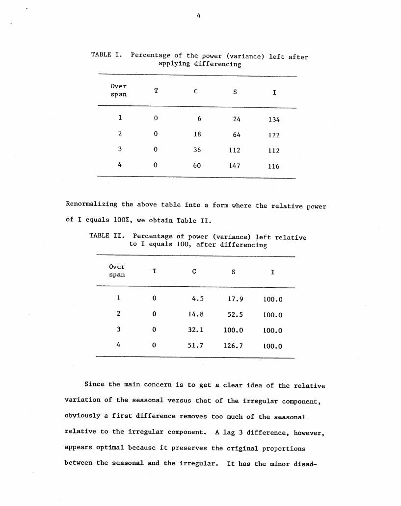
;,;:;

13

.~~

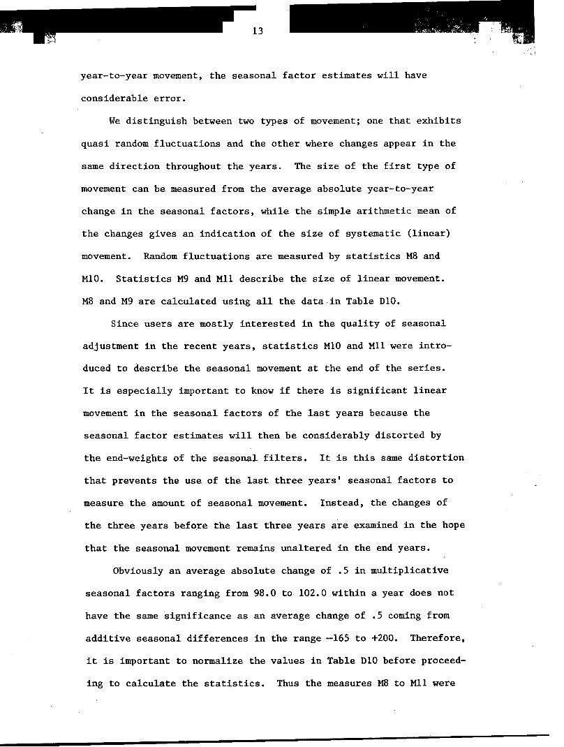
year-to-year movement, the seasonal factor estimates will have

considerable error.

We distinguish between two types of movement; one that exhibits

quasi random fluctuations and the other where changes appear in the

same direction throughout the years. The size of the first type of

movement can be measured from the average absolute year-to-year

change in the seasonal factors, while the simple arithmetic mean of

the changes gives an indication of the size of systematic (linear)

movement. Random fluctuations are measured by statistics M8 and

M10. Statistics M9 and M11 describe the size of linear movement.

M8 and M9 are calculated using all the data-in Table DI0.

Since users are mostly interested in the quality of seasonal

adjustment in the recent years, statistics MiO and MIl were intro-

duced to describe the seasonal movement at the end of the series.

It is especially important to know if there is significant linear

movement in the seasonal factors of the last years because the

seasonal factor estimates will then be considerably distorted by

the end-weights of the seasonal filters. It is this same distortion

that prevents the use of the last three years' seasonal factors to

measure the amount of seasonal movement. Instead, the changes of

the three years before the last three years are examined in the hope

that the seasonal movement remains unaltered in the end years.

Obviously an average absolute change of .5 in multiplicative

seasonal factors ranging from 98.0 to 102.0 within a year does not

have the same significance as an average change of .5 coming from

additive seasonal differences in the range -165 to +200. Therefore,

it is important to normalize the values in Table D10 before proceed-

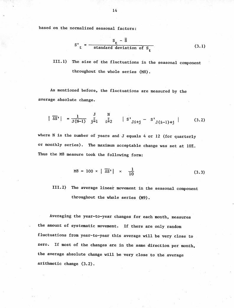
ing to calculate the statistics. Thus the measures M8 to MIl were

-'j;"

'.J!~;~F:~ "- 16 -

When MIl exceeds I, there is strong indication that the seasonal fc..: .",;

~factors for recent years are highly distorted due to the flattening

effect of the end weights on linear movements.

IV. GENERAL COMMENTS ON THE OVERALL QUALITY OF THE ADJUSTMENT

The eleven statistics each examine a different facet of the

adjustment and no one statistic can judge the overall quality of

the adjustment. Also, each statistic has been developed for an

average series and thus might break down for an unusual series.

It is possible that the series fails the M1 or M2 statistic

and the adjustment does not necessarily suffer. These two

statistics measure the irregular variation in proportion to the

seasonal variation. The average series adjusted has a cycle which

contributes about 5 to 10% to the stationary portion of the

variance. The threshold level for the M1 and M2 statistics is

based on this assumption. If the series contains no cycle, the

irregular can contribute 13 to 14% to the total variation (resulting

in M1 and M2 values exceeding 1) and still be acceptable. Similarly, ..

if the cycle contributes more than 10%, the threshold level should

be lowered.

If a series has a flat (i.e. almost constant) trend-cycle, it

is possible to have an r/c ratio exceeding 3 and thus failing the

M3 test, without jeopardizing the quality of the adjustment.

Actually, the X-II program compensates for the lack of trend by

applying a 23-term Henderson moving average to estimate the trend-

cycle. However, if the user's main objective is business cycle.

analysis a high M3 value signals a serious problem. It indicates

that the final seasonally adjusted series contains a very high-

.:,!i-I7;.'~

proportion of irregular movement that will prevent users fromI

properly identifying the trend-cycle component.

Finding significant autocorrelation in the final irregulars

as indicated by an M4 value greater than 1, can signal, for example,

that the user should have applied trading-day regression and thus the

adjustment is not valid. At the same time it is possible that the

original irregulars were auto correlated due to the sampling design.

This will not affect the X-Ii seasonal adjustment that is based on

recognizing characteristic seasonal and trend-cycle behaviour in a

series and obtains the irregulars as the residuals of the procedure.

Thus the correct seasonal factor can still be well identified. It

was found that the measure M4 moved rather independently from the

other measures and quite often it was the only statistic that failed

or one of the very few that did not fail. Consequently, it was not

as related to the quality of seasonal adjustment as the others and

was assigned a minimum weight.

In the case of MS, what was said about M3 applies again. It

is possible that the irregulars are too high but it is also con-

ceivable that the series contains an almost constant trend-cycle

which does not. prevent X-li from isolate out the right seasonal 5('

movement.

As pointed out before, M6 is the only statistic where failure

can be corrected. The user is advised to rerun X-Ii and apply the

appropriate seasonal moving average to the 81 series in order to

improve the quality of seasonal adjustment.

Any series that fails the statistic M7 has either no season-

ality or the seasonal estimates are so distorted that the seasonal

component is not identifiable as indicated in the message after

Table D8. This measure is the most important one in the set of

18

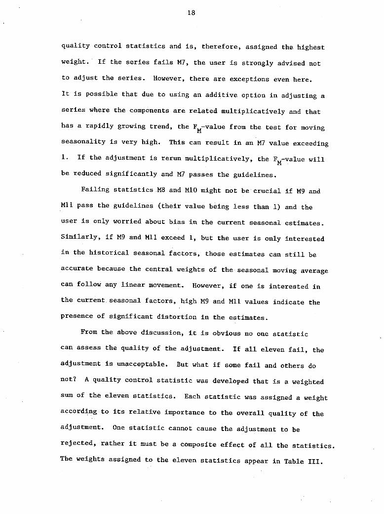
quality control statistics and is, therefore, assigned the highest

weight. If the series fails M7, the user is strongly advised not

to adjust the series. However, there are exceptions even here.

It is possible that due to using an additive option in adjusting a

series where the components are related multiplicatively and that

has a rapidly growing trend, the FM-value from the test for moving

seasonality is very high. This can result in an M7 value exceeding

1. If the adjustment is rerun multiplicatively, the FM-value will

be reduced significantly and M7 passes the guidelines.

Failing statistics M8 and MIa might not be crucial if M9 and

MIl pass the guidelines (their value being less than 1) and the

user is only worried about bias in the current seasonal estimates.

Similarly, if M9 and MIl exceed 1, but the user is only interested

in the historical seasonal factors, those estimates can still be

accurate because the central weights of the seasonal moving average

can follow any linear movement. However, if one is interested in

the current seasonal factors, high M9 and MIl values indicate the

presence of significant distortion in the estimates.

From the above discussion, it is obvious no one statistic

can assess the quality of the adjustment. If all eleven fail, the

adjustment is unacceptable. But what if some fail and others do

not? A quality control statistic was developed that is a weighted

sum of the eleven statistics. Each statistic was assigned a weight

according to its relative importance to the overall quality of the

adjustment. One statistic cannot cause the adjustment to be

rejected, rather it must be a composite effect of all the statistics.

The weights assigned to the eleven statistics app~ar in Table III.

19

TABLE III. The Standard Eleven M Weights

Statistics(Mi) Weight (w.)1

M1 13M2 13M3 10M4 5M5 11M6 10M7 16M8 7M9 7M10 4MIl 4

The eleven statistics can sometimes take values less than

zero or greater than three. If this happens the statistic is set

to be zero or three respectively. Thus the quality control

statistic Q is defined as:

11E w.Mi. 1 1Q = 1= (4.1)

11E w.. 1 1

1=

If the user selects a seasonal moving average different from

a (3 x 5) for estimating the seasonal factors, the statistic M6 is

not relevant.. Thus under these conditions:

w = o. (4.2)6

If the series is less than 6 years long, or the stable seasonal

option is chosen, the statistics M8, M9, MiO and MIl cannot be

calculated and the weights are redefined as displayed in Table IV

21

If the Q statistic is greater than 1, the adjustment of the

series is declared to be unacceptable. The adjustment is also

rejected if the test for identifiable seasonality fails. For

quarterly series 11.0% of the series failed the Q statistic and an ;.-

additional 1% failed the test for identifiable seasonality. For

monthly series, 8.4% had Q-values higher than 1 and an additional 3.7%

were rejected because they did not pass the test for identifiable

seasonality. Overall 12.1% of the 421 seasonal adjustments were

rejected. The 51 series that failed were examined in detail by

the authors and for all of them, the adjustment was deemed to be

unacceptable. The quality control statistics presented here will

enable users with a large number of series to quickly assess the

quality of all their adjustments as well as enable people with

little knowledge of seasonal adjustment to make judgements on the

acceptability of the results. The Q statistic provides a general

assessment of the quality of the adjustment, but the users should

beware of attaching significance to small changes in the statistic.

This especially holds for aggregate adjustments as shown in

Appendix A.

At the back of each printout produced by the X-11-ARIMA

program, appears a summary of the Q statistics for all the series

adjusted in that run. Thus, the quality of large numbers of series

can be quickly judged. I1IUnediately after the Q statistics are :' ,

copies of the F2 and F3 tables of all the series run. If any

series has produced an unacceptable adjustment, the user can turn

to the F2 and F3 tables for that series and further identify the

problem. Following this procedure, hundreds of series can be

assessed in less than an hour.

.22

APPENDIX A

QUALITY ASSESSMENT OF AGGREGATE SERIES

The new X-l1-ARIMA program can automatically produce direct

and indirect aggregate seasonal adjustments of several component

series. The preceding quality control statistics are produced for

both the direct and indirect adjustment. The Q statistics for

the two methods can be used to assess the acceptability of the

adjustment for both methods. Unfortunately, the Q statistics

cannot be used to judge which of the two methods gives a superior

adjustment. The Q's for the two types of adjustments are usually

very close to each other and small differences in the Q's cannot be

interpreted as being significant. The M8 and M1Q statistics for

the indirect method will generally be greater than for the direct.

This will tend to make the Q for the indirect method greater than

for direct. This creates a bias in the Q statistic against indirect

adjustments.

Additional summary statistics are produced if an aggregate

adjustment is requested. These statistics are printed on the same

page as the summary of all the Q statistics for the series adjusted.

This summary appears right after the printout of the last series.

The comparison test for the direct versus the indirect seasonal

adjustment method is based on a paper by Lothian and Morry (1977).

The statistic tests the degree of smoothness of the seasonally

adjusted series. The standard deviation of the month-to-month (or

quarter-to-quarter) changes in the two seasonally adjusted series

23

is computed for the whole series and for the last three years of

the series. The standard deviation of the direct differences is

then subtracted from the indirect for both the whole series and

the last three years. If the resulting differences are positive,

the indir~ct method gives a smoother adjustment than the direct

method. If they are negative, the direct method results in a

smoother seasonally adjusted series. It is also possible that the

results for the last three years disagree with those of the full

series. The differences are normalized by dividing by the average

value of the seasonally adjusted series and multiplying by 100 to

get the percentage difference between the direct and indirect

methods.

,

24

REFERENCES

Bradley, James V. (1968): Distribution-Free Statistical Tests,

Prentice Hall, Englewood Cliffs, N.J.

Higginson, John (1975): "An F test for the Presence of Moving

Seasonality when Using Census Method II-X-1I Variant"

Research Paper, Seasonal Adjustment and Time Series Staff,

Statistics Canada.

Huot, Guy and de Fontenay, Allain (1973): "General Sea-sonal

Adjustment Guidelines, Statistics Canada version of the X-II

Program", Research Paper, Seasonal Adjustment and Time Series

Staff, Statistic~ Canada.

Lothian, John (1978): "The Identification and Treatment of Moving

Seasonality in the X-II-ARIMA Seasonal Adjustment Program",

Research Paper, Seasonal Adjustment and Time Series Staff,

Statistics Canada.

Lothian, John and Morry, Marietta (1978): "A Test for Identifiable

Seasonality When Using the X-I1-ARIMA Program", Research Paper,

Seasonal Adjustment and Time Series Staff, Statistics Canada.

Lothian, John and Morry, Marietta (1977): "The Problem of Aggrega-

tion; Direct or Indirect" Research Paper, Seasonal Adjustment

and Time Series Staff, Statistics Canada.

Shiskin, J., Young, A.H. and Musgrave, J.C. (1967): "The X-II

Variant of Census Method II, Seasonal Adjustment", Technical

Paper No. 15, Bureau of the Census, u.S. Dept. of Commerce

Wallis, W.A. and Moore, G.H. (1941): "A Significance Test for

Time Series", National Bureau of Economic ReseaEch, Technical

Paper No.1.

-