a semiparametric multivariate, multisite weather …...a semiparametric multivariate, multisite...

A semiparametric multivariate, multisite weather generator withlow-frequency variability for use in climate risk assessments

Scott Steinschneider1 and Casey Brown1

Received 4 February 2013; revised 9 September 2013; accepted 11 September 2013; published 4 November 2013.

[1] A multivariate, multisite daily weather generator is presented for use in decision-centricvulnerability assessments under climate change. The tool is envisioned to be useful for awide range of socioeconomic and biophysical systems sensitive to different aspects ofclimate variability and change. The proposed stochastic model has several components,including (1) a wavelet decomposition coupled to an autoregressive model to account forstructured, low-frequency climate oscillations, (2) a Markov chain and k-nearest-neighbor(KNN) resampling scheme to simulate spatially distributed, multivariate weather variablesover a region, and (3) a quantile mapping procedure to enforce long-term distributionalshifts in weather variables that result from prescribed climate changes. The Markov chain isused to better represent wet and dry spell statistics, while the KNN bootstrap resamplerpreserves the covariance structure between the weather variables and across space. Thewavelet-based autoregressive model is applied to annual climate over the region and used tomodulate the Markov chain and KNN resampling, embedding appropriate low-frequencystructure within the daily weather generation process. Parameters can be altered in any ofthe components of the proposed model to enable the generation of realistic time series ofclimate variables that exhibit changes to both lower-order and higher-order statistics atlong-term (interannual), mid-term (seasonal), and short-term (daily) timescales. The toolcan be coupled with impact models in a bottom-up risk assessment to efficiently andexhaustively explore the potential climate changes under which a system is mostvulnerable. An application of the weather generator is presented for the Connecticut Riverbasin to demonstrate the tool’s ability to generate a wide range of possible climatesequences over an extensive spatial domain.

Citation: Steinschneider, S., and C. Brown (2013), A semiparametric multivariate, multisite weather generator with low-frequencyvariability for use in climate risk assessments, Water Resour. Res., 49, 7205–7220, doi:10.1002/wrcr.20528.

1. Introduction

[2] The reluctance of the global community to mitigategreenhouse gas emissions and the legacy of past emissionsalready produced spurs the need for climate change adapta-tion. Recently, bottom-up or ‘‘decision-centric’’ approachesto identifying robust climate change adaptations havebecome more popular in the literature [Jones, 2001; John-son and Weaver, 2009; Lempert and Groves, 2010; Prud-homme et al., 2010; Wilby and Dessai, 2010; Brown et al.,2011; Brown and Wilby, 2012]. These approaches focus ona system of interest (e.g., agricultural lands, an ecosystem,a reservoir, etc.) and systematically identify its vulnerabil-ities to climate; this contrasts ‘‘scenario-led’’ methods that

limit the analysis to a set of climate model projections thatmay or may not reveal a system’s climate sensitivities. Acritical step in decision-centric methods involves testingthe performance of a system over a range of plausible cli-mate changes to identify harmful climate states that couldcause the system to fail. As the literature on this topic isrelatively young, limited tools have been investigated forthe production of altered climate time series over which toconduct the vulnerability assessment. This study presents anew stochastic weather generator specifically designed toaid these assessments. The model can be used to generatetime series of weather expressing various changes in theclimate at multiple temporal scales. Such time series maybe especially useful for exploring changes that are expectedto occur, such as increasing intensity and decreasing fre-quency of precipitation consistent with the acceleration ofthe hydrologic cycle, or changes to low-frequency climatevariability, that are not well simulated in current global cli-mate model projections.

[3] Bottom-up or vulnerability-based approaches to cli-mate change adaptation form a relatively new area ofresearch that attempts to appraise possible adaptations of asystem to climate stressors by first identifying the climatevulnerabilities of that system over a wide range of potentialclimate changes. After system vulnerabilities are identified,

Additional supporting information may be found in the online version ofthis article.

1Department of Civil and Environmental Engineering, University ofMassachusetts Amherst, Amherst, Massachusetts, USA.

Corresponding author: S. Steinschneider, Department of Civil and Envi-ronmental Engineering, University of Massachusetts Amherst, 130 NaturalResources Rd., Amherst, MA 01002, USA. ([email protected])

©2013. American Geophysical Union. All Rights Reserved.0043-1397/13/10.1002/wrcr.20528

7205

WATER RESOURCES RESEARCH, VOL. 49, 7205–7220, doi:10.1002/wrcr.20528, 2013

different adaptation strategies can be evaluated over threat-ening climate states in order to identify robust adaptationmeasures. The likelihood of harmful climate conditions canalso be assessed using available climate information,including the most up-to-date climate modeling results(e.g., global circulation model (GCM) projections). Bydetaching the identification of system vulnerabilities fromclimate projections produced by GCMs, bottom-upapproaches differ from more traditional top-downapproaches that depend on a limited number of internallyconsistent climate scenarios to explore the range of poten-tial climate change impacts [Christensen et al., 2004;Wiley and Palmer, 2008]. It has been argued that bottom-up methods are better equipped to provide more decision-relevant information useful in identifying robust adaptationmeasures under deep future uncertainty [Lempert et al.,1996]. In part, this is because bottom-up approaches canbetter explore a full range of plausible climate changes,whereas GCM projections provide only a limited view anddo not delimit the possible range (although they are ofteninterpreted to do so) [see Stainforth et al., 2007; Deseret al., 2012].

[4] Despite the growing interest in decision-centricapproaches, technical methods for actually conducting thevulnerability assessment (i.e., generating perturbed climatesequences over which to test system vulnerability) are rela-tively underdeveloped. To date, only a handful of methodshave been utilized. The most popular approach has been toapply simple change factors to the historic record of precip-itation and temperature, effectively testing system sensitiv-ities to mean climate shifts [Johnson and Weaver, 2009;Gober et al., 2010; Lempert and Groves, 2010; Brownet al., 2012]. Other studies have explored more detailedchanges, including shifts in intraannual climate [Prud-homme et al., 2010] and high-order statistics (e.g., variance,serial correlation) of annual hydroclimate data [Moody andBrown, 2013]. While all of these approaches were appropri-ate for their specific application, these methods exhibit lim-ited ability to perturb the entire distribution of climatevariables or alter their behavior at multiple temporal scales.For instance, none of the methods mentioned are equippedto simulate climates exhibiting shifts in both long-term(decadal) precipitation persistence and extreme daily pre-cipitation amounts. Yet both of these changes are possibleunder climate change [Timmermann et al., 1999; Collins,2000; Intergovernmental Panel on Climate Change, 2007]and may be important in a climate sensitivity analysis for aparticular system (e.g., a reservoir jointly managed forflood risk reduction and water supply). Thus, there is aneed for more generalized and comprehensive tools to con-duct climate vulnerability assessments for systems sensitiveto different climate variables across multiple temporalscales.

[5] We propose stochastic weather generators as onepossible tool that can fulfill this need. Stochastic weathergenerators are computer algorithms that produce long seriesof synthetic daily weather data. The parameters of themodel are conditioned on existing meteorological recordsto ensure the characteristics of historic weather emerge inthe daily stochastic process. Weather generators are a popu-lar tool for extending meteorological records [Richardson,1985], supplementing weather data in a region of data spar-

sity [Hutchinson, 1995], disaggregating seasonal hydrocli-matic forecasts [Wilks, 2002], and downscaling coarse,long-term climate projections to fine-resolution, dailyweather for impact studies [Wilks, 1992; Kilsby et al.,2007; Groves et al., 2008; Fatichi et al. 2011, 2013]. Theiruse for climate sensitivity analysis of impact models hasalso been tested, particularly in the agricultural sector[Semenov and Porter, 1995; Mearns et al., 1996; Riha etal. 1996; Dubrovsky et al. 2000; Confalonieri, 2012].These sensitivity studies systematically change parametersin the model to produce new sequences of weather varia-bles (e.g., precipitation) that exhibit a wide range of changein their characteristics (e.g., average amount, frequency, in-tensity, duration, etc.). By incrementally manipulating oneor more parameters in the model, many climate scenarioscan be simulated that exhaustively explore potential futuresthat exhibit slight differences in nuanced climate character-istics, such as the intensity and frequency of daily precipi-tation, the serial correlation of extreme heat days, or therecurrence of long-term droughts. Previous bottom-up cli-mate impact assessments, which have relied heavily onsimple change factors to generate new climate sequences,have not been able to test system vulnerabilities over sucha wide range of plausible climate changes. To the authors’knowledge, only one study has used a weather generator toinvestigate a system’s climate sensitivity in the context of adecision-centric climate change analysis [Jones, 2000], andthis study only examined changes in mean temperature andprecipitation. The potential of weather generators for driv-ing vulnerability assessments in bottom-up climate changestudies has not yet been adequately explored, particularlywith respect to nuanced aspects of climate variability.

[6] While the use of stochastic weather generators forbottom-up risk assessments is very attractive in theory,there are many challenges that arise in practical applica-tion. As mentioned earlier, socioeconomic and biophysicalsystems are often vulnerable not only to changes in meanclimate but also to changes in nuanced climate variability.Therefore, the chosen weather generator should be able toeasily perturb any of these climate characteristics, whichnot all models in the literature can easily accomplish [Wilksand Wilby, 1999]. Additionally, impact models oftenrequire sequences of several weather variables at multiplelocations that exhibit a realistic covariance structurebetween variables and across sites. The production of spa-tially distributed, correlated weather variables continues tochallenge certain approaches to stochastic weather genera-tion [Beersma and Buishand, 2003]. Weather variables canalso exhibit long-term persistence [Hurst, 1951; Kout-soyiannis, 2003] on timescales up to decades that can sig-nificantly impact system performance, requiring that thechosen weather generator be capable of replicating (andpossibly altering in a bottom-up analysis) structured low-frequency climate variability.

[7] The literature is rich with examples of stochasticweather generators that can address some subset of thechallenges listed above. Both parametric and nonparamet-ric models have been proposed to maintain correlationstructures between variables and across sites [Wilks, 1998,1999; Rajagopalan and Lall, 1999; Buishand andBrandsma, 2001; Wilby et al., 2003, Apipattanavis et al.,2007]. Some have argued that nonparametric models may

STEINSCHNEIDER AND BROWN: WEATHER GENERATOR FOR CLIMATE RISK

7206

be more capable than their parametric counterparts toreproduce the spatial covariance structure of multivariateweather variables [Buishand and Brandsma, 2001], but theability to specify distributional shifts in weather variablesis often more straightforward using parametric approaches[Wilks and Wilby, 1999]. Several models have also beenproposed to preserve low-frequency variability observed inthe historic record [Hansen and Mavromatis, 2001;Dubrovsky et al., 2004; Wang and Nathan, 2007; Chenet al., 2010; Fatichi et al. 2011; Kim et al., 2011], but theseapproaches have not been generalized to multisite applica-tions. After a substantial literature review, the authors wereonly able to identify one stochastic weather generator inthe literature with the ability to specify distributional shiftsin weather variables while simultaneously maintaininglow-frequency climate variability and intervariable andintersite correlations [Srikanthan and Pegram, 2009], andthe simulation of multidecadal climate persistence may stillbe difficult with this model formulation. In the context ofvulnerability based climate change assessments, a newmodel is required that can simultaneously simulate weathervariables exhibiting accurate correlations between variablesand across sites, appropriate long-term persistence at inter-annual and interdecadal time scales, and shifted distribu-tional characteristics hypothesized under climate change.

[8] This study presents a stochastic weather generator withgreater ability to support bottom-up vulnerability assessmentsunder climate change for a wide range of socioeconomic andbiophysical systems sensitive to different aspects of climatevariability and change. The proposed stochastic modeladdresses all of the challenges mentioned above with severalcomponents, including (1) a wavelet decomposition coupledto an autoregressive model to account for structured, low-frequency climate oscillations, (2) a Markov chain andk-nearest-neighbor (KNN) resampling scheme to simulatespatially distributed, multivariate weather variables over aregion, and (3) a quantile mapping procedure to enforcelong-term distributional shifts in weather variables under cli-mate change. Parameters that govern each model componentcan be altered to perturb various statistics of the climate sys-tem at different temporal scales. The tool can be coupledwith impact models in a decision-centric risk assessment todetermine the potential climate changes under which a sys-tem is most vulnerable. This allows the analyst to evaluatesystem performance over a wide range of possible climatechanges to identify risk or to investigate specific climatechange effects that are of concern (e.g., less frequent butmore intense rainfall). An application of the weather genera-tor is presented for the Connecticut River basin to demon-strate the tool’s ability to generate a wide range of possibleclimate sequences over an extensive spatial domain. The re-mainder of the paper proceeds as follows. The proposedweather generator is presented in section 2. The model isevaluated in section 3, and section 4 demonstrates the abilityof the model to produce various climate sequences for use ina bottom-up climate change analysis. The article then con-cludes with a discussion in section 5.

2. The Weather Generator

[9] A flexible weather generator is desired that canaccurately reproduce various characteristics of the historic

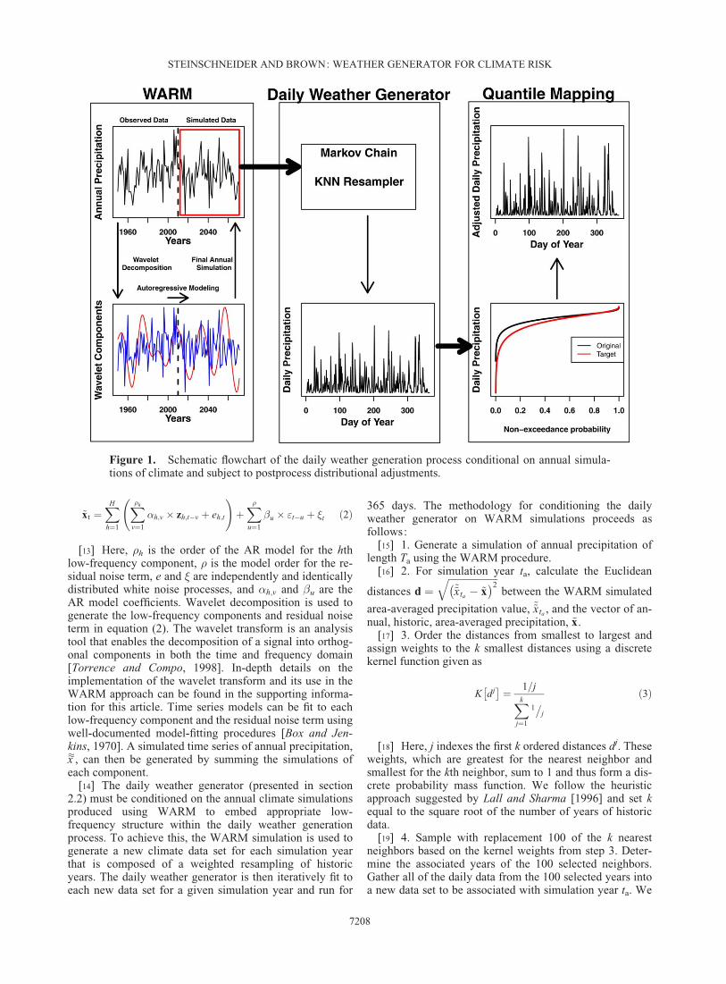
climate regime while introducing the capacity to altermany of these characteristics in a decision-centric climatechange analysis. The model considered in this work cou-ples an autoregressive wavelet decomposition [Kwon etal., 2007] for extracting and simulating low-frequencystructure in annual climate with a multivariate weathergenerator [Apipattanavis et al., 2007] that effectively cap-tures daily weather characteristics, including dry and wetspell statistics, cross correlations between weather varia-bles, and spatial correlations across multiple sites. Thetwo models are linked by conditioning the daily weathergenerator on simulations of annual climate produced bythe autoregressive wavelet decomposition. Time series ofweather variables produced by the coupled modelingapproach are then altered in a third step used to enforcedistributional shifts in the climate. For precipitation, aquantile mapping procedure is utilized to implement thischange. Long-term shifts in other variables are enforcedusing simpler additive and scaling methods. A flow dia-gram of the overall modeling framework is given in Fig-ure 1. The various submodels and algorithms used aredescribed in detail below.

2.1. Wavelet Autoregressive Model for thePreservation of Low-Frequency Structure

[10] Most daily weather generators produce weather sim-ulations that tend to be overdispersed at interannual time-scales and fail to reproduce observed low-frequencypersistence. Several studies have proposed methods to cor-rect for overdispersion in weather simulations [Hansen andMavromatis, 2001; Dubrovsky et al., 2004; Wang andNathan, 2007; Chen et al., 2010; Fatichi et al. 2011; Kimet al., 2011]. This study utilizes a relatively new approachput forth in Kwon et al. [2007] that extracts low-frequencysignals in climate data using wavelet decomposition andthen stochastically simulates each signal using autoregres-sive time series models. By simulating each signal sepa-rately, the wavelet autoregressive model (WARM) canbetter reproduce a time series of climate exhibiting a simi-lar spectral signature to the observed data. In our methodol-ogy, the WARM approach is applied to annual, area-averaged precipitation over the region of interest. Eachyear of generated annual precipitation is then used toinform a single-year simulation of the daily weather gener-ator (described below), embedding appropriate low-frequency structure within the daily weather generationprocess.

[11] Let ~x represent a time series of annual, area-averaged precipitation for a region. The WARM approachdecomposes this series into H orthogonal component series,zh, that represent different low-frequency signals, as wellas a residual noise component e.

~x ¼XH

h¼1

zh þ E ð1Þ

[12] A simulation of ~x is generated with time series mod-els of each low-frequency component and the residualnoise. Following Kwon et al. [2007], we consider linearautoregressive (AR) models for each term:


7207

~xt ¼XH

h¼1

X�h

v¼1

�h;v � zh;t�v þ eh;t

!þX�u¼1

�u � "t�u þ �t ð2Þ

[13] Here, �h is the order of the AR model for the hthlow-frequency component, � is the model order for the re-sidual noise term, e and � are independently and identicallydistributed white noise processes, and �h;v and �u are theAR model coefficients. Wavelet decomposition is used togenerate the low-frequency components and residual noiseterm in equation (2). The wavelet transform is an analysistool that enables the decomposition of a signal into orthog-onal components in both the time and frequency domain[Torrence and Compo, 1998]. In-depth details on theimplementation of the wavelet transform and its use in theWARM approach can be found in the supporting informa-tion for this article. Time series models can be fit to eachlow-frequency component and the residual noise term usingwell-documented model-fitting procedures [Box and Jen-kins, 1970]. A simulated time series of annual precipitation,x�, can then be generated by summing the simulations ofeach component.

[14] The daily weather generator (presented in section2.2) must be conditioned on the annual climate simulationsproduced using WARM to embed appropriate low-frequency structure within the daily weather generationprocess. To achieve this, the WARM simulation is used togenerate a new climate data set for each simulation yearthat is composed of a weighted resampling of historicyears. The daily weather generator is then iteratively fit toeach new data set for a given simulation year and run for

365 days. The methodology for conditioning the dailyweather generator on WARM simulations proceeds asfollows:

[15] 1. Generate a simulation of annual precipitation oflength Ta using the WARM procedure.

[16] 2. For simulation year ta, calculate the Euclidean

distances d ¼ffiffiffiffiffiffiffiffiffiffiffiffiffiffiffiffiffiffiffiffi~~xta � ~x� �2

qbetween the WARM simulated

area-averaged precipitation value, ~~xta , and the vector of an-nual, historic, area-averaged precipitation, ~x.

[17] 3. Order the distances from smallest to largest andassign weights to the k smallest distances using a discretekernel function given as

K dj� �¼ 1=jXk

j¼1

1j

� ð3Þ

[18] Here, j indexes the first k ordered distances dj. Theseweights, which are greatest for the nearest neighbor andsmallest for the kth neighbor, sum to 1 and thus form a dis-crete probability mass function. We follow the heuristicapproach suggested by Lall and Sharma [1996] and set kequal to the square root of the number of years of historicdata.

[19] 4. Sample with replacement 100 of the k nearestneighbors based on the kernel weights from step 3. Deter-mine the associated years of the 100 selected neighbors.Gather all of the daily data from the 100 selected years intoa new data set to be associated with simulation year ta. We

Figure 1. Schematic flowchart of the daily weather generation process conditional on annual simula-tions of climate and subject to postprocess distributional adjustments.


7208

note that data may be repeated in this new data set becauseyears can be sampled more than once.

[20] 5.Build the daily weather generator using this condi-tional data set and run it over the length of 1 year.

[21] 6. Repeat steps 1–5 for all Ta years of the annualWARM simulation.

2.2. Semiparametric Multivariate and MultisiteWeather-Generating Algorithm

[22] The daily weather generation process utilized in thisstudy is based on the methods proposed in Apipattanavis etal. [2007]. That study coupled a Markov chain and KNNresampling scheme to simulate spatially distributed, corre-lated, multivariate weather variables over a region. TheMarkov chain is used to better represent wet and dry spellstatistics while the KNN bootstrap resampler preserves thecovariance structure between the weather variables andacross space. Since the details of the method can be foundin Apipattanavis et al. [2007], only a brief overview will beprovided here.

[23] Assume a simulated, daily time series of R weather

variables Xl ¼ xl1;t; x

l2;t; :::; x

lR;tjt ¼ 1; 2; :::; T

n ois desired

at L different locations, where xli;t represents the ith weather

variable (e.g., precipitation) at time t and location l, and Tis the length of the simulation. A weather generationscheme is designed to simulate area-averaged weather vari-ables, X, that can then be immediately disaggregated toindividual locations. The weather generation approach isbased on the common practice of first simulating precipita-tion occurrence, St, as a chain-dependent process. A three-state (extremely wet (St¼2), wet (St¼1) or dry (St¼0)) Mar-kov chain of order 1 is used to simulate the occurrence ofarea-averaged precipitation across the L locations. Thenumber of states and chain order can be chosen to maxi-mize performance while maintaining model parsimonyusing quantitative criteria such as Akaike’s information cri-terion [Akaike, 1974], though this study simply follows thechain structure suggested in Apipattanavis et al. [2007].Nine transition probabilities (p00, p01, p02, p10, p11, p12, p20,

p21, p22) for the three-state Markov chain are fit to the area-averaged precipitation occurrence time series by monthusing the method of maximum likelihood. Here, pab

denotes the probability of precipitation state b occurring,given the occurrence of state a on the previous day. Athreshold of 0.3 mm is chosen to distinguish between wetand dry days at the area-averaged scale, while the 80th per-centile of area-averaged precipitation (by month) is used asthe threshold for extremely wet conditions. Again, thesevalues are taken directly from Apipattanavis et al. [2007].

[24] Area-averaged precipitation occurrence can besimulated from the fitted Markov chain using standard pro-cedures well documented in the previous weather genera-tion literature. After simulating the occurrence of area-averaged precipitation states, a vector of weather variablesX must be simulated and then disaggregated to each of theL locations. A KNN resampling algorithm of lag-1 is usedto generate the values for all the weather variables. Thisalgorithm follows a six-step process:

[25] 1. Let Xt�1 be a vector of area-averaged weathervariables already simulated for day t�1. Also assume,

without loss of generality, that the Markov chain had simu-lated day t�1 and day t as wet days.

[26] 2. Partition the historic record to find all pairs ofdays in a 7 day window centered on day t (if day t is 15 Jan-uary, then the window includes all historic days from 12 to18 January) that have the same sequence of area-averagedprecipitation states simulated by the Markov chain for dayt�1 and day t (in this case, two wet days in a row). Assumethere are Q such pairs, each containing 2 days of area-

averaged weather, X1q and X

2q.

[27] 3. Calculate the weighted Euclidean distance, dq,between the simulated, area-averaged vector of weathervariables, Xt�1, and each of the Q vectors of historic, area-averaged variables:

dq ¼

ffiffiffiffiffiffiffiffiffiffiffiffiffiffiffiffiffiffiffiffiffiffiffiffiffiffiffiffiffiffiffiffiffiffiffiffiffiffiffiffiffiffiffiffiffiffiffiffiffiffiffiffiffiffiffiffiffiffiffiffiffiffiffiffiffiffiffiffiffiffiffiffiffiffiffiffiffiXR

i¼1

wi � xi;t�1 � xi

� �� x1

i;q � xi

� � 2

vuut ð4Þ

[28] Here, xi;t�1 denotes the ith area-averaged weathervariable already simulated for time t�1, x1

i;q denotes thesame area-averaged weather variable on the first day of theqth historic pair sampled in step 2, xi is the mean of the itharea-averaged weather variable across all time steps, and wi

denotes the weight. In this study, each weight wi is setequal to the inverse of the standard deviation of the ithweather variable, though there are methods in the literaturefor selecting weights in KNN resampling procedures toproduce optimal forecasts [Karlsson and Yakowitz, 1987].By centering each variable in the distance equation aboutits mean and dividing by its standard deviation, we stand-ardize values and give near-equal importance to each vari-able in the nearest-neighbor calculation. Prior tonormalization, transformations may be required for non-Gaussian weather variables.

[29] 4. Order the distances dq from smallest to largest.The k smallest distances are assigned weights using thesame discrete kernel function presented in equation (3).Again, we follow the heuristic approach suggested by Lalland Sharma [1996] and set k ¼

ffiffiffiffiQp

.[30] 5. Sample one of the k-nearest neighbors based on

the weights developed in step 4 and record the historic dateassociated with that selected neighbor. Then, use vectors ofweather variables Xl on the successive day to the recordeddate for each of the L locations to simulate the multivariate,multisite weather for day t.

[31] 6. Repeat steps 1–5 for all T days of the simulation.[32] To begin the algorithm and generate initial values

for all weather variables, data for a random day from thesimulation starting month is selected from the historic re-cord that is consistent with the first precipitation state simu-lated by the Markov chain.2.3. Quantile Mapping Technique to Enforce Long-Term Climate Changes

[33] By just using the coupled models of sections 2.1 and2.2, it is not feasible to generate weather outside of the rangeof historic variability, nor is it possible to change the distribu-tion of those variables. In the context of a vulnerability assess-ment, this capability is critically important, particularly forprecipitation, which often dominates system performance. Theapproach developed here incorporates a quantile mapping


7209

method to alter the distribution of daily precipitation. Altera-tions to other weather variables are treated more simply usingstandard additive or multiplicative factors.

[34] Let X̂m;l

p be daily, nonzero precipitation values formonth m and location l simulated from the daily weather gen-erator. Assume the simulated precipitation amounts can bemodeled by a theoretical cumulative distribution functionF

X̂m;lp

x0jgð Þ with parameters g. A ‘‘target’’ cumulative distribu-

tion function, F�X̂

m;lp

x0jg�ð Þ, is introduced that represents the

projected distribution of future precipitation under a climatechange. For simplicity, we assume that F

X̂m;lp

and F�X̂

m;lp

arise

from the same distribution but differ between their parametersets, g and g

�. The parameter set g

�can be altered to control

how the distribution of future precipitation differs from the his-toric observations. Many possible changes in precipitationcharacteristics are possible through adjustments to g

�, includ-

ing shifts in the mean, standard deviation, or extremes. Forexample, assume historic and projected precipitation for monthm follow two-parameter Gamma distributions with shape andscale parameters g¼ {�, �} and g

� ¼ {��, ��}. The parameter

set g can be estimated by fitting a Gamma distribution to X̂m;l

p .

Then, a new mean �� and variance 2� can be specified forthe target Gamma distribution, and the parameter set g

�can be

inferred using the relationships between the parameters andthe first two moments, �� ¼ �� and 2� ¼ �� 2�. Ifchanges in the first two moments do not sufficiently accountfor particular shifts in higher order statistics that are of interest,the target parameter set g

�can be further tailored to better

impose this change. Once the parameter set g�

of the targetdistribution is specified, a quantile mapping procedure can beused to alter the distribution F

X̂m;lp

of simulated nonzero precip-

itation to match that specified by F�X̂

m;lp

(Figure 2). To do this,

we first determine the exceedance probability of the tth valueof synthesized precipitation for month m, x̂m;l

p;t , from the cdf

FX̂

m;lp

. Then, the target cdf F�X̂

m;lp

is used to map this exceedance

probability to a new precipitation amount, ðx̂m;lp;t Þ�, that is con-

sistent with the specified distribution for climate-alteredmonthly precipitation:

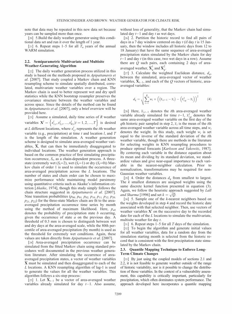
Figure 2. The quantile mapping procedure to adjust daily, nonzero precipitation values. (a) A sampleof an original time series of April precipitation simulated by the weather generator. The blue point repre-sents a sample precipitation value to be adjusted. (b) The cdf for the fitted gamma distribution to theoriginal simulation of April precipitation (black), as well as the target cdf used to make the adjustments(red). (c) The rectangle delimits an inset, shown in detail. Here, the precipitation value represented bythe blue point in Figure 2a is mapped to a new precipitation value via four steps. (d) The new, adjustedprecipitation time series, including the adjusted point (blue), is shown.


7210

x̂m;lp;t

� �¼ F�

X̂m;lp

�1 FX̂

m;lp

x̂m;lp;t

� �ð5Þ

[35] This procedure is repeated for each nonzero precipi-tation amount synthesized by the weather generator.

3. Model Evaluation

[36] To evaluate the performance of the proposedweather generator, we apply it to daily weather data distrib-uted across the Connecticut River basin in the New Eng-land region of the United States. Daily precipitation andmaximum and minimum temperature are the variablesincluded in the analysis. The data are available between 1January 1949 and 31 December 2010 as gridded observa-tions with a spatial resolution of approximately 144 km2

[Maurer et al., 2002]. The Connecticut River basin drainsover 31,000 km2 and contains a large number (260) of gridcells, enabling an evaluation of the multisite performanceof the approach. The spatial extent of the proposed modelapplication is quite large, and so adequate performance ofthe model at this spatial scale greatly supports its use forvulnerability assessments of large, spatially expansive sys-tems. For evaluation, the model is run 50 separate times,each 62 years long (the length of the historic record). Weexamine the reproduction of multiple characteristics ofeach weather variable at several different time scales.

[37] Figure 3 shows the mean, standard deviation, andskew of nonzero daily precipitation amounts, daily maxi-

mum temperature, and daily minimum temperature for allcombinations of months and grid cells. The median valuesof these statistics are taken over the 50 different simula-tions for comparison against the historic statistics. Theresults suggest good performance for all variables and sta-tistics except for the skew of daily precipitation, whichtends to be underestimated in the simulations for some gridcells.

[38] Correlations of a given variable across sites and crosscorrelations between different variables for a given site areshown in Figure 4. Again, median values across the 50 simu-lations are shown. Both types of correlation are very wellpreserved, as is expected given the resampling techniquesused to generate the daily weather sequences. The simula-tions also capture the average number of dry and wet daysacross all sites and months rather well (Figure 5). There is aslight underestimation of the average lengths of wet and dryspells, particularly for those grid cells with larger spelllengths, but this underestimation is slight (less than a day).

[39] The spread of lag-1 autocorrelations across the 50different simulations are shown in Figure 6. For each vari-able, the distribution of this statistic is shown for the averageautocorrelation across all sites. There is a negative bias inthe lag-1 autocorrelations for daily precipitation, althoughthis bias is slight. Similarly, the simulations tend to consis-tently underestimate the autocorrelation in the temperaturefields, but again this bias is actually rather small in magni-tude. The slight underestimation of serial correlation for all

Figure 3. Daily performance statistics for all grid cells and months, including the mean, standard devi-ation, and skew of precipitation, maximum temperature, and minimum temperature. Median valuesacross the 50 different simulations are shown against the observed values.


7211

variables could likely be improved by increasing the orderof the Markov chain, but no such correction was made here.

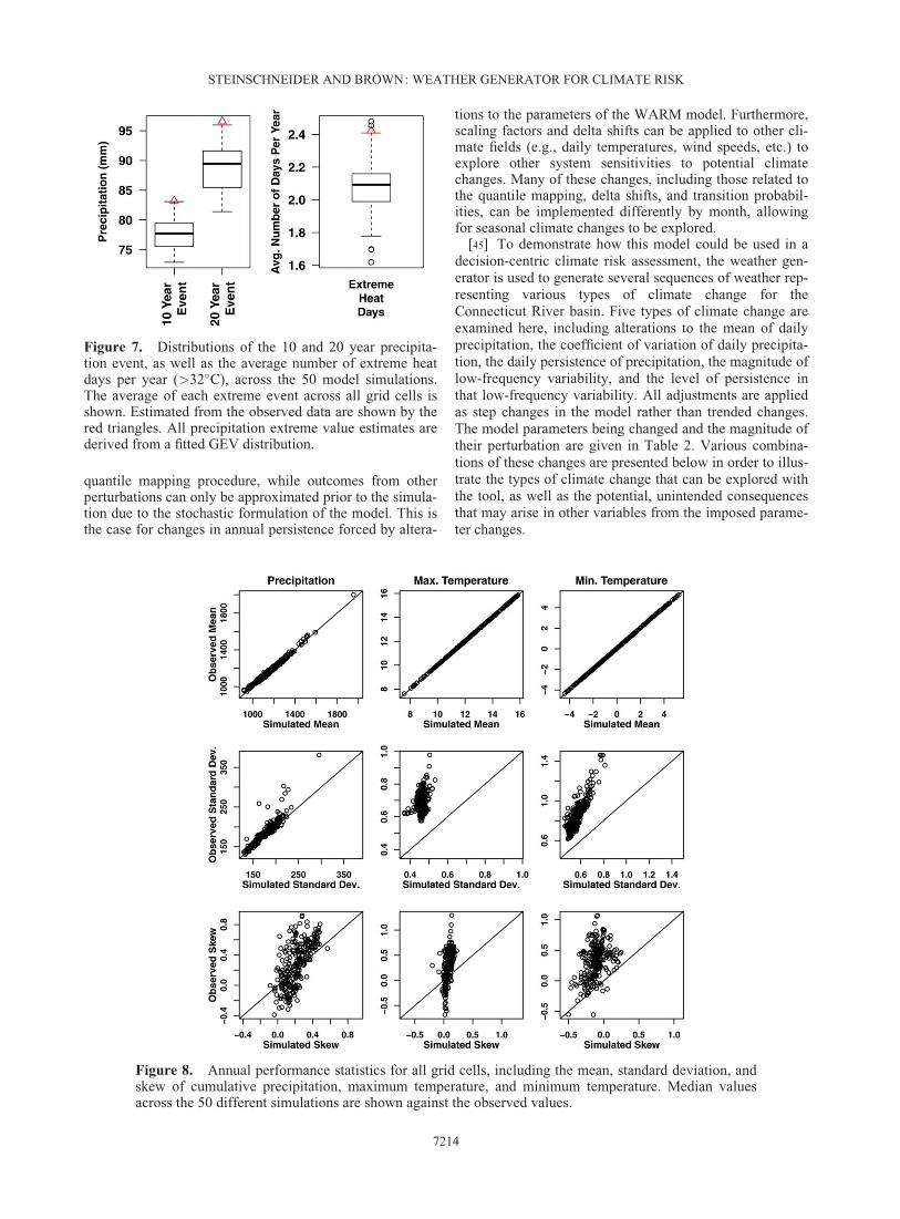
[40] To explore the reproduction of extremes, Figure 7shows the distribution of 10 and 20 year maximum annualprecipitation events, as well as the average number ofextreme heat days, across the 50 simulations. The precipita-tion extreme value estimates were developed for each gridcell by fitting a Generalized Extreme Value (GEV) distribu-tion to the time series of annual maximum precipitation atthat location. The temperature extremes were taken as the av-erage number of days per year above 32�C. The distributionsfor the average of these statistics across all locations areshown for the ensemble of 50 simulations. The model tendsto underestimate the magnitude of extreme rainfall events,although the spread of model simulations contains theobserved value for the 10 year event and nearly reaches theobserved value for the 20 year event. For temperatureextremes, the model again shows a slight negative bias,although the range of simulations does contain the observedvalue. Overall, there is a moderate negative bias in theextremes, an effect that can often emerge in weather genera-tors that rely on data resampling [Lee et al., 2012].

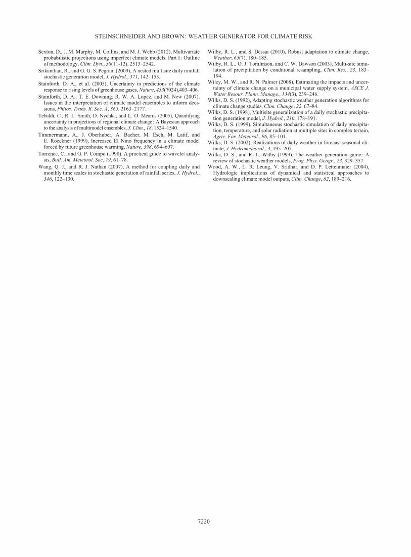
[41] Statistical comparisons for annual precipitationtotals and temperature averages are shown in Figure 8. Themean precipitation and temperature fields are well pre-served at the annual timescale. The standard deviation ofprecipitation is adequately captured for all but a few grid

cells. The standard deviation of both temperature fieldstends to be undersimulated, particularly for those grid cellsexhibiting greater annual temperature variability. The skewfor all three variables is not well captured by the model,although we note that there is significant uncertainty in theobserved skew values due to the small number of annualobservations available for its calculation. For precipitationand maximum temperature, the skew is overestimated forthose grid cells with small skew values and underestimatedfor those grid cells with larger skew values. This particularmodel discrepancy may be due to the fact that basin-averaged climate fields are being used to drive the modelover a large and somewhat heterogeneous region.

[42] Finally, the power spectra of annual precipitationvalues are examined in Figure 9. One low-frequency com-ponent (H¼1) with significant periods between 1 and 4years was modeled in the WARM approach. The meansimulated power spectrum across the 50 simulationsmatches that seen for the observations reasonably well.Most importantly, the mean simulated spectra become stat-istically insignificant at around the same period length (�4years) as in the observations. Furthermore, the observedspectra are completely within the 95% uncertainty bounds.

[43] Overall, the performance of the model for most sta-tistics is either good or adequate, with only some moderatediscrepancies in the higher-order statistics. This is promis-ing given that the model is being applied to a very large

Figure 4. Intersite correlations for daily precipitation, maximum temperature, and minimum tempera-ture, as well as cross correlations between each pair of variables. Median values across the 50 differentsimulations are shown against the observed values for all grid cells. Correlations are taken across theentire simulation/observed record.


7212

region subject to various changes in topography, which canoften be quite challenging for weather generation proce-dures. Furthermore, we note that these performance statis-tics are comparable to those seen in the weather generatorpresented in Srikanthan and Pegram [2009], which is theonly other weather generator in the literature with the abil-ity to specify distributional shifts in weather variableswhile simultaneously maintaining low-frequency climatevariability and intervariable and intersite correlations.

4. Model Demonstration for a Climate StressTest

[44] The daily weather generator was specificallydesigned to facilitate a decision-centric climate risk assess-ment of systems sensitive to several components of the cli-mate at various temporal scales. In the modelingframework presented here an emphasis was placed on alter-ing precipitation patterns in the climate system because thisvariable often dominates the performance of biophysicaland socioeconomic systems. Several parameters can beadjusted in the model to vary different components of pre-cipitation (see Table 1). These include the parameters forthe target distribution in the quantile mapping scheme, thetransition probabilities of the Markov chain, the coeffi-cients of the AR model for low-frequency components, and

the standard deviation of white noise for those AR models.By changing these parameters, shifts in daily precipitationamounts, daily persistence, interannual persistence, andinterannual variability can be implemented in a bottom-upclimate change assessment. The exact outcome of some ofthese perturbations will be known a priori, such as with the

Figure 5. Average number of dry and wet days per month, as well as the average dry and wet spelllength per month, across all grid cells. Median values across the 50 different simulations are shownagainst the observed values.

Figure 6. Distributions of lag 1 serial correlation valuesfor precipitation and maximum and minimum temperatureacross the 50 model simulations. The average serial corre-lation across all grid cells is shown. Observed values areshown by the red triangles. All serial correlations are takenacross the entire simulation/observed record.


7213

quantile mapping procedure, while outcomes from otherperturbations can only be approximated prior to the simula-tion due to the stochastic formulation of the model. This isthe case for changes in annual persistence forced by altera-

tions to the parameters of the WARM model. Furthermore,scaling factors and delta shifts can be applied to other cli-mate fields (e.g., daily temperatures, wind speeds, etc.) toexplore other system sensitivities to potential climatechanges. Many of these changes, including those related tothe quantile mapping, delta shifts, and transition probabil-ities, can be implemented differently by month, allowingfor seasonal climate changes to be explored.

[45] To demonstrate how this model could be used in adecision-centric climate risk assessment, the weather gen-erator is used to generate several sequences of weather rep-resenting various types of climate change for theConnecticut River basin. Five types of climate change areexamined here, including alterations to the mean of dailyprecipitation, the coefficient of variation of daily precipita-tion, the daily persistence of precipitation, the magnitude oflow-frequency variability, and the level of persistence inthat low-frequency variability. All adjustments are appliedas step changes in the model rather than trended changes.The model parameters being changed and the magnitude oftheir perturbation are given in Table 2. Various combina-tions of these changes are presented below in order to illus-trate the types of climate change that can be explored withthe tool, as well as the potential, unintended consequencesthat may arise in other variables from the imposed parame-ter changes.

Figure 7. Distributions of the 10 and 20 year precipita-tion event, as well as the average number of extreme heatdays per year (>32�C), across the 50 model simulations.The average of each extreme event across all grid cells isshown. Estimated from the observed data are shown by thered triangles. All precipitation extreme value estimates arederived from a fitted GEV distribution.

Figure 8. Annual performance statistics for all grid cells, including the mean, standard deviation, andskew of cumulative precipitation, maximum temperature, and minimum temperature. Median valuesacross the 50 different simulations are shown against the observed values.


7214

[46] Figures 10a and 10b show the changes to the distri-bution of nonzero daily precipitation at one grid cell inApril caused by increasing the mean and coefficient of vari-ation, respectively, for that month by 30% in the quantilemapping procedure. All other components of the climatesystem were kept unchanged from their historic, fitted val-ues. Comparisons are made against a baseline model runwith no changes imposed. When the mean value isincreased in the quantile mapping approach, the entire dis-tribution of daily precipitation values is shifted upward(Figure 10a). These values are shifted in such a way toensure that the variability of precipitation (i.e., the coeffi-cient of variation) does not change. Correlations betweenprecipitation and maximum temperature are examined todetermine whether mean changes under the quantilemapping procedure degrade relationships between precipi-

tation and other variables (Figure 10d). For mean changes,these relationships appear well preserved. The distributionof daily April precipitation looks quite different when themean is kept constant but the coefficient of variation isincreased (Figure 10b). Here, the distribution is stretched toincrease the highest events (>0.85 nonexceedance level)while lowering all of the remaining, smaller precipitationvalues in order to maintain the same mean value. Thisstretching of the distribution causes distortions in the corre-lations between precipitation and temperature, producing anegative bias in the correlation values across most gridcells (Figure 10e).

[47] Figure 10c shows the average number of dry daysper month across all grid cells for a model run under base-line transition probabilities in the Markov chain and a runwith increased persistence in dry days. As expected, the runwith a greater persistence in dry days exhibits an increasednumber of these events. Unlike the results from the quantilemapping procedure, however, the change in this statisticfor each grid cell can only be determined after imposingthe alternative model parameterization and exploring theresulting climate sequence, because daily precipitation per-sistence is being modeled (and altered) at the basin-averagescale. We also note that alterations to daily precipitationpersistence can change the distribution of certain tempera-ture statistics that depend on the occurrence of precipita-tion. For instance, increases in dry day persistence also leadto more extreme heat days (>32�C) across most grid cells(Figure 10f).

[48] Finally, we present a sample of model runs exhibit-ing changes to the magnitude, variability, and frequency ofannual precipitation. The model runs are compared againstan ensemble of GCM projections to demonstrate how theweather generator can produce a much wider range ofpotential climate changes than the limited view afforded bythe GCMs. Figure 11 shows the mean, coefficient of varia-tion, and lag-1 autocorrelation coefficient for annual pre-cipitation averaged over the entire Connecticut River basin.The statistics from several climate scenarios are presented,including those from the observed record, 234 downscaledGCM projections for the 2050–2099 period, and many dif-ferent weather generator runs. The GCM projections weregathered from the World Climate Research Program’s(WCRP’s) Coupled Model Intercomparison Project phase 5(CMIP5) multimodel data set and were downscaled usingthe bias-correction spatial disaggregation technique [Wood

Table 1. Model Parameters That Can Be Altered to Perturb the Climate System at Various Temporal Scales

Climate Field Model Component Parameter Effect

Timing

Daily SeasonalInterannual/Interdecadal

Precipitation Quantile mapping Target distributionparameters (g

�)

Change entire distribution of dailyprecipitation by month

X X

Daily weathergenerator

Transitionprobabilities (pab)

Alter the daily persistence of dailyprecipitation by month

X X

WARM Coefficients of theAR model (�h)

Adjust the persistence oflow-frequency signals

X

WARM Standard deviation ofAR white noise (e)

Adjust the magnitude oflow-frequency signals

X

Temperature Daily WeatherGenerator

Delta Shifts (t) Shift the daily temperaturevalues by month

X X

Figure 9. Power spectra for annual precipitation. Theobserved spectra (black solid) are compared against themean power spectra (dashed blue) of the 50 simulations,along with range bounded by the 2.5th and 97.5th percen-tiles of the power spectra for the ensemble (gray). Alsoshown is the 95% significance level (red dotted) developedfrom a red noise background process. The power spectra ofthe observations and simulations become statistically sig-nificant if they rise above the red dotted line.


7215

et al., 2004; Reclamation, 2013]. Three, 20 memberensembles of weather generator runs, each 62 years long,are presented. The first set is run under baseline conditions,while the second set is run with a 30% reduction in meanprecipitation and a 30% increase in the standard deviationof annual precipitation. The final ensemble is run with a30% increase in mean precipitation, a 30% reduction in thestandard deviation of annual precipitation, and a significant

decrease in the lag-1 autocorrelation of annualprecipitation.

[49] Several conclusions emerge from the results in Fig-ure 11. First, the ensemble of 2050–2099 GCM runs showsan increase in mean precipitation over the historic average,with a mean increase of 110% and a range of 100% and122%. These projections show a slight decline in the aver-age coefficient of variation, but this change is largely

Figure 10. Intended (first row) and unintended (second row) changes to various weather characteristicsdue to forced changes in model parameters, including the mean of daily precipitation (first column), thecoefficient of variation (CV) (second column), and transition probabilities in the Markov chain (thirdcolumn). Comparisons are made between a model run with the change imposed and a baseline run with-out any parameter changes. (a, b) Baseline (black solid) and adjusted (red dashed) empirical distributionsof nonzero April precipitation for a single grid cell. (c) The average number of dry days per month acrossall grid cells. (d, e) The cross correlation between nonzero precipitation and maximum temperature ateach grid cell. (f) The average number of extreme heat days (>32�C) per year across all grid cells.

Table 2. Climate Changes Included in the Stress Testa

Climate Change Model Parameter Adjusted Size of Adjustmentb

Mean precipitation Mean of daily precipitation (��) 630%

Precipitation variability Coefficient of variation of daily precipitation �

��

� þ30%

Daily precipitation persistence Transition probabilities p0,1 and p0,0 �0.2 (p0,1)þ0.2 (p0,0)

Magnitude of low-frequency variability Standard deviation of white noise for all AR models (e, �) 630%Persistence of low-frequency variability Lag-1 coefficient for low-frequency component (�1) �0.2

aAll adjustments are applied as step changes in the model rather than trended changes.bAll values show the size of the change above baseline values.


7216

driven by an increase in the mean with little change in thestandard deviation. Also, the projections exhibit muchlower serial correlation values than that seen in theobserved record, with only a handful of scenarios showingcomparable levels of persistence. The historic (1950–2000)time period from these projections (not shown) exhibit thesame low level of persistence as the future scenarios, sug-gesting that the downscaled GCM projections may not ex-hibit realistic, higher-order climate characteristics over anaggregate region. Importantly, the magnitude, variability,and persistence of annual precipitation under these futureGCM projections only exhibit a limited range of possibleoutcomes. This narrow view of possible future climate out-comes limits the utility of these projections in a climatechange risk analysis, in which all climate possibilities, par-ticularly high-impact, low-probability events, are importantto the discovery and quantification of risk.

[50] In contrast, the 20 member ensemble of weathergenerator runs under baseline conditions exhibit climatecharacteristics that are directly comparable to the observedrecord. The magnitude, variability, and lag-1 autocorrela-tion of annual precipitation are all relatively unbiased. Fur-thermore, the ensemble of runs presents a range ofplausible climates that could occur even without climatechange, providing an analyst with climate sequences thatcould be used to test the robustness of a system to internalclimate variability.

[51] A much wider range of possible future outcomescan be explored using the proposed weather generator. Fig-ure 11 exhibits two possible combinations of change simu-lated by the model, including a set of climate sequenceswith significantly less but more variable annual precipita-tion, as well as a set of climate sequences with more annualprecipitation, but with depressed variability and persist-ence. These two sets of changes are just a sample of whatcould be simulated by the weather generator, but their ex-pansive range across climate change space demonstrateshow the model could be used to explore a wide range ofpossible climate outcomes under climate change. Thisaffords analysts more flexibility in how they examine theweaknesses of a system of interest and enables a more thor-ough exploration of climate risk. Given the tendency ofplanners and managers to underestimate the possibility ofpotential hazards, we feel that there are significant advan-tages to exploring system weaknesses over a wide range ofpossible climate outcomes, an analysis made possible bythe proposed weather generator.

5. Discussion

5.1. Model Limitations

[52] It is important to recognize the limitations of anytool when trying to infer insight from model results. Whilethe weather generator presented in this study was designedto simulation multiple forms of climate variability at sev-eral different time scales, there are certain components ofclimate variability that are still challenging for the model toaccount for or modulate. For one, a resampling algorithmdrives the model, so at the daily time scale the tool implic-itly assumes that the spatial correlation structure of theweather variables is stationary. This may not be the caseunder future climate changes, yet such a change cannot be

simulated with this model. At interannual timescales, thetool currently simulates low-frequency variability based onan annual precipitation time series and ignores any signalin the annual temperature data. Also, it may be difficult toestimate robust parameters for certain low-frequency sig-nals in the WARM model if the length of the annual precip-itation time series is not sufficiently long. One approach tocircumvent both of these issues would be to replace the an-nual precipitation time series with an alternative climateproxy that relates to both precipitation and temperature(such as an ENSO index), for which there is more dataavailable through climate reconstructions [Kwon et al.,2009]. This requires, however, that a significant climateproxy with a long record can be found for the region of in-terest. Additionally, if monotonic trends, as opposed toquasi-oscillatory variability, are present in the annual data,then the WARM approach may identify spurious low-frequency components [Kwon et al. 2007]. Such trends, ifidentified, should be removed from the data before buildingthe WARM model, but distinguishing trends from low-frequency oscillations is not straightforward. Finally, thismodel is data intensive, and therefore may be difficult touse in data-sparse regions. Despite these limitations, how-ever, this tool does provide a step forward in the simulation

Figure 11. The mean, coefficient of variation, and lag-1serial correlation coefficient of annual precipitation. Statis-tics for several climate scenarios are shown, including (1)the observed record (red), (2) future (brown) BCSD down-scaled GCM projections from the CMIP5 archive, (3) 20baseline weather generator simulations (blue), (4) 20 simu-lations with a decreased mean and increased standard devia-tion (green), and (5) 20 simulations with an increased mean,decreased standard deviation, and decreased autocorrelation(magenta). The observed lag-1 serial correlation is 0.19.


7217

of climate across multiple temporal and spatial scales foruse in vulnerability assessments of human and ecologicalsystems.

5.2. Determining Scenario Plausibility, Selecting theScenario Range, and Linking to Climate Science

[53] The model presented here was designed to supportdecision-centric climate change studies by enabling an ana-lyst to test a system under a wide range of plausible climatescenarios and identify potential climate hazards. However,the analyst faces two immediate questions when trying toconduct this ‘‘climate stress test’’ : (1) what constitutes aplausible climate change? and (2) how large should therange of climate changes be? Finding limitations on howfar the climate can be perturbed before the scenario shouldbe considered implausible is a difficult task. Expert opinionmay be useful in defining these bounds, as may very largesimulation ensembles of simpler (computationally faster)climate models [Piani et al. 2005]. However, the plausibil-ity of each climate change scenario may not be criticalwhen identifying system hazards as long as implausiblechanges are discounted or disregarded later in the analysiswhen developing estimates of climate risk [Brown et al.,2012]. The important factor is to determine how far the cli-mate must change before the system no longer functionsproperly so that the analyst is aware of the potential climatehazards. Therefore, a promising strategy in bottom-upapproaches may be to identify those climate variables andtime scales that influence the performance of the systemand then extend the range of climate changes for those vari-ables wide enough to stress the system to failure. Whenthose failures emerge, judgments can be made regardingthe plausibility of the conditions causing them; they neednot be made earlier. In practice, there may be computa-tional challenges for exploring so many scenarios, but withparallel computing capabilities, the cost of an additionalsimulation run is often rather small. Also, adaptive sam-pling techniques may be utilized to reduce the number ofsimulations needed to discover performance thresholds inclimate change space.

[54] Once performance thresholds in climate changespace are identified, information on the likelihood of harm-ful climate states can be used to estimate climate risks fac-ing the system. If certain scenarios used in the stress testare truly implausible, then the likelihood assessment shouldreveal this and discount these scenarios when estimatingclimate risk. Downscaled GCM projections are a logicalstarting place to garner this likelihood information, andrecently, there have been significant efforts in the climatescience community to develop formal probability distribu-tions of global and regional climate variables from theseprojections. These approaches utilize initial conditionensembles [Stainforth et al., 2005], perturbed physicsensembles [Rougier et al., 2009], multimodel ensembles[Tebaldi et al., 2005], or combinations thereof [Sexton etal., 2012] to develop pdfs of response variables. Expertopinion can also be valuable in forming these likelihoodestimates, as can data from the paleorecord. In addition,imprecise probabilities could be utilized to express uncer-tainty regarding the estimated values [Rinderknecht et al.,2012]. Potentially, more reliable probability estimates maybe developed for discrete thresholds (i.e., the likelihood of

climate change beyond a threshold associated with systemfailure), rather than continuous probabilities across theentire climate space. In all of these cases, the probabilitiesof change should likely be considered subjective, but theycan still be coupled with the results of the vulnerabilityassessment to quantitatively appraise the robustness of dif-ferent adaptation measures across the range of climatechange space [Moody and Brown, 2013]. More research isneeded to explore approaches for gathering this probabilis-tic information and coupling it with the results of an exten-sive vulnerability assessment.

6. Conclusion

[55] The most recent scientific knowledge suggests thatthe impacts of climate change on socioeconomic and bio-physical systems could be very significant, yet they remainhighly uncertain. Recently, decision-analytic approacheshave been proposed to better handle this uncertainty andframe adaptation studies under climate change in termsmore relevant for decision makers. These approaches, oftenbottom-up by design, require an understanding of systemsensitivities to various changes in the climate system to bet-ter identify vulnerabilities and develop an understanding ofpotential risks to the system. However, technical methodsfor conducting these vulnerability assessments are rela-tively underdeveloped in the literature. This study pre-sented a stochastic weather generator that can helpfacilitate the discovery of system vulnerabilities to severalcomponents of the climate system. When coupled withimpact models, the weather generator enables a more com-plete identification of system vulnerabilities that can helpinform risk management strategies and the selection ofrobust adaptation measures.

[56] The tool is designed to work not only for specificsites but also for systems that cover large spatial extents,such as trans-state river basins or ecosystems. However,future work is needed to explore how spatially expansivethe model can be made before its skill degrades. Futurestudies will also utilize the weather generator tool to con-duct stress tests on various socioeconomic and biophysicalsystems in order to appraise potential improvements fromavailable adaptation measures.

[57] As climatic records continue to show increasingnonstationary in their probabilistic behavior, decision mak-ers across a range of fields will seek actionable informationthat directly informs a choice between measures they cantake to safeguard their system from further shifts in the cli-mate. The high degree of uncertainty that surrounds thesechanges hinders the utility of a traditional predict-then-actframework for adaptation decision making. A shift in phi-losophy may be needed to provide the information trulyneeded to adapt our society to potential environmentalchanges that we cannot foresee. This study hopefully addsto a developing body of literature exploring new methodsto analyze and present climate change adaptation informa-tion that can help better inform decision makers as theynavigate an uncertain future.

[58] Acknowledgments. We thank three anonymous reviewers fortheir thoughtful criticisms and advice that helped to significantly improvethis article. The work of the authors was partially supported by the


7218

National Science Foundation grant CBET-1054762 and the Department ofDefense Strategic Environmental Research and Development Program(SERDP) project RC-2204.

ReferencesAkaike, H. (1974), A new look at the statistical model identification, IEEE

Trans. Automat. Contr., 19, 716–723.Apipattanavis, S., G. Podesta, B. Rajagopalan, and R. W. Katz (2007), A

semiparametric multivariate and multisite weather generator, WaterResour. Res., 43, W11401, doi:10.1029/2006WR005714.

Beersma, J. J., and T. A. Buishand (2003), Multi-site simulation of dailyprecipitation and temperature conditional on the atmospheric circulation,Clim. Res., 25, 121–133.

Box, G. E.P., and G. Jenkins (1970), Time Series Analysis, Forecasting,and Control, Holden-Day, Boca Raton, Fla.

Brown, C., and R. L. Wilby (2012), An alternate approach to assessing cli-mate risks, Eos Trans. AGU, 93(41), 401–402, doi:10.1029/2012EO410001.

Brown, C., Y. Ghile, M. Laverty, and K. Li, (2012) Decision scaling: Link-ing bottom-up vulnerability analysis with climate projections in the watersector, Water Resour. Res. 48, W09537, doi:10.1029/2011WR011212.

Brown, C., W. Werick, W. Leger, and D. Fay (2011), A decision-analyticapproach to managing climate risks: Application to the Upper GreatLakes, J. Am. Water Resour. Assoc., 47(3), 524–534, doi:10.1111/j.1752-1688.2011.00552.x.

Buishand, T. A., and T. Brandsma (2001), Multisite simulation of daily pre-cipitation and temperature in the Rhine basin by nearest-neighbor resam-pling, Water Resour. Res., 37(11), 2761–2776.

Chen, J., F. P. Brissette, and R. Leconte (2010), A daily stochastic weathergenerator for preserving low-frequency of climate variability, J. Hydrol.,388, 480–490.

Christensen, N. S., A. W. Wood, N. Voisin, D. P. Lettenmaier, and R. N.Palmer (2004), The effects of climate change on the hydrology and waterresources of the Colorado River Basin, Clim. Change, 62, 337–363.

Collins, M. (2000), Understanding uncertainties in the response of ENSO togreenhouse warming, Geophys. Res. Lett., 27(21), 3509–3512,doi:10.1029/2000GL011747.

Confalonieri, R. (2012), Combining a weather generator and a standard sen-sitivity analysis method to quantify the relevance of weather variables onagrometeorological model outputs, Theor. Appl. Climatol., 108, 19–30,doi:10.1007/s00704-011-0510-0.

Deser, C., A. Phillips, V. Bourdette, and H. Teng, (2012), Uncertainty inclimate change projections: The role of internal variability. Clim. Dyn.,38(3-4), 527–546.

Dubrovsky, M., Z. Zalud, and M. Stastna (2000), Sensitivity of ceres-maizeyields to statistical structure of daily weather variables, Clim. Change,46, 447–472.

Dubrovsky, M., J. Buchtele, and Z. Zalud (2004), High-frequency and low-frequency variability in stochastic daily weather generator and its effecton agricultural and hydrologic modeling, Clim. Change, 63, 145–179.

Fatichi, S., V. Y. Ivanov, and E. Caporali (2011), Simulation of future cli-mate scenarios with a weather generator, Adv. Water Resour., 34(4),448–467.

Fatichi, S., V. Y. Ivanov, and E. Caporali (2013), Assessment of a stochas-tic downscaling methodology in generating an ensemble of hourly cli-mate time series, Clim. Dyn., 40(7-8), 1841–1861.

Gober, P., C. W. Kirkwood, R. C. Balling Jr., A. W. Ellis, and S. Deitrick(2010), Water planning under climatic uncertainty in Phoenix: Why weneed a new paradigm, Ann. Assoc. Am. Geogr., 100(2), 356–372.

Groves, D. G., D. Yates, and C. Tebaldi (2008), Developing and applyinguncertain global climate change projections for regional water managementplanning, Water Resour. Res., 44, W12413, doi:10.1029/2008WR006964.

Hansen, J. W., and T. Mavromatis (2001), Correcting low-frequency vari-ability bias in stochastic weather generators, Agric. For. Meteorol., 109,297–310.

Hurst, H. E. (1951), Long term storage capacities of reservoirs, Trans. Am.Soc. Civil Eng., 116, 776–808.

Hutchinson, M. F. (1995), Stochastic space-time models from ground-based data, Agric. For. Meteorol., 73, 237–264.

Intergovernmental Panel on Climate Change (2007), Climate Change2007: The Physical Basis, Contributions of Working Group I to theFourth Assessment Report of the Intergovernmental Panel on ClimateChange, edited by S. Solomon et al., Cambridge Univ. Press, Cambirdge,U. K.

Johnson, T. E., and C. P. Weaver (2009), A framework for assessing cli-mate change impacts on water and watershed systems, Environ. Man-age., 43, 118–134.

Jones, R. N. (2000), Analyzing the risk of climate change using an irriga-tion demand model, Clim. Res., 14, 89–100.

Jones, R. N. (2001), An environmental risk assessment/management frame-work for climate change impact assessments, Natl. Hazards, 23, 197–230.

Karlsson, M., and S. Yakowitz (1987), Nearest-neighbor methods for non-parametric rainfall-runoff forecasting, Water Resour. Res., 23(7), 1300–1308, doi:10.1029/WR023i007p01300.

Kilsby, C. G., P. D. Jones, A. Burton, A. C. Ford, H. J. Fowler, C. Harpham,P. James, A. Smith, and R. L. Wilby (2007), A daily weather generatorfor use in climate change studies, Environ. Modell. Software, 22, 1705–1719.

Kim, Y., R. W. Katz, B. Rajagopalan, G. P. Podesta, and E. M. Furrer(2011), Reducing overdispersion in stochastic weather generators using ageneralized linear modeling approach, Clim. Res., 53, 13–24.

Koutsoyiannis, D. (2003), Climate change, the Hurst phenomenon, andhydrologic statistics, Hydrol. Sci. J., 48(1), 3–24.

Kwon, H.-H., U. Lall, and A. F. Khalil (2007), Stochastic simulation modelfor nonstationary time series using an autoregressive wavelet decomposi-tion: Applications to rainfall and temperature, Water Resour. Res., 43,W05407, doi:10.1029/2006WR005258.

Kwon, H.-H., U. Lall, and J. Obeysekera (2009), Simulation of daily rain-fall scenarios with interannual and multidecadal climate cycles for SouthFlorida, Stochastic Environ. Res. Risk Assess., 23, 879–896.

Lall, U., and A. Sharma (1996), A nearest neighbor bootstrap for time seriesresampling, Water Resour. Res., 32(3), 679–693.

Lee, T., T. B.M. J. Ouarda, and C. Jeong (2012), Nonparametric multivari-ate weather generator and an extreme value theory for bandwidth selec-tion, J. Hydrol., 452-453, 161–171.

Lempert, R. J., and D. G. Groves (2010), Identifying and evaluating robustadaptive policy responses to climate change for water management agen-cies in the American west, Technol. Forecast. Social Change, 77, 960–974.

Lempert, R. J., M. E. Schlesinger, and S. C. Bankes (1996), When we don’tknow the costs or the benefits: Adaptive strategies for abating climatechange, Clim. Change, 33(2), 235–274.

Maurer, E. P., A. W. Wood, J. C. Adam, D. P. Lettenmaier, and B. Nijssen(2002), A long-term hydrologically-based data set of land surface fluxesand states for the conterminous United States, J. Clim., 15, 3237–3251.

Mearns, L. O., C. Rosenzweig, and R. Goldberg (1996), The effect ofchanges in daily and interannual climatic variability on ceres-wheat: Asensitivity study, Clim. Change, 32, 257–292.

Moody, P., and C. Brown (2013), Robustness indicators for evaluationunder climate change: Application to the upper Great Lakes, WaterResour. Res., 49, 3576–3588, doi:10.1002/wrcr.20228.

Piani, C., D. J. Frame, D. A. Stainforth, and M. R. Allen (2005), Constraintson climate change from a multi-thousand member ensemble of simula-tions, Geophys. Res. Lett. 32, L23825, doi:10.1029/2005GL024452.

Prudhomme, C., R. L. Wilby, S. Crooks, A. L. Kay, and N. S. Reynard(2010), Scenario-neutral approach to climate change impact studies:Application to flood risk, J. Hydrol., 390, 198–209, doi:10.1016/j.jhydrol.2010.06.043.

Rajagopalan, B., and U. Lall (1999), A k-nearest-neighbor simulator fordaily precipitation and other weather variables, Water Resour. Res.,35(10), 3089–3101.

Reclamation, (2013), Downscaled CMIP3 and CMIP5 climate and hydrol-ogy projections: Release of downscaled CMIP5 climate projections,comparison with preceding information, and summary of user needs, 47pp., U.S. Dep. of the Interior, Bureau of Reclamation, Technical ServicesCenter, Denver, Colo.

Richardson, C. W. (1985), Weather simulation for crop management mod-els, Trans. Am. Soc. Agric. Eng., 28, 1602–1606.

Riha, S. J., D. S. Wilks, and P. Simoens (1996), Impact of temperature andprecipitation variability on crop model predictions, Clim. Change, 32,293–311.

Rinderknecht, S. L., M. E. Borsuk, and P. Reichert (2012), Bridging uncer-tain and ambiguous knowledge with imprecise probabilities, Environ.Modell. Software, 36, 122–130.

Rougier, J., D. Sexton, J. M. Murphy, and D. Stainforth (2009), Analyzingthe climate sensitivity of the HadSM3 climate model using ensemblesfrom different but related experiments, J. Clim., 22(13), 3540–3557.

Semenov, M. A., and J. R. Porter (1995), Climatic variability and the mod-eling of crop yields, Agric. For. Meteorol., 73(3-4), 265–283.


7219

Sexton, D., J. M. Murphy, M. Collins, and M. J. Webb (2012), Multivariateprobabilistic projections using imperfect climate models. Part I : Outlineof methodology, Clim. Dyn., 38(11-12), 2513–2542.

Srikanthan, R., and G. G. S. Pegram (2009), A nested multisite daily rainfallstochastic generation model, J. Hydrol., 371, 142–153.

Stainforth, D. A., et al. (2005), Uncertainty in predictions of the climateresponse to rising levels of greenhouse gases, Nature, 433(7024),403–406.

Stainforth, D. A., T. E. Downing, R. W. A. Lopez, and M. New (2007),Issues in the interpretation of climate model ensembles to inform deci-sions, Philos. Trans. R. Soc. A, 365, 2163–2177.

Tebaldi, C., R. L. Smith, D. Nychka, and L. O. Mearns (2005), Quantifyinguncertainty in projections of regional climate change: A Bayesian approachto the analysis of multimodel ensembles, J. Clim., 18, 1524–1540.

Timmermann, A., J. Oberhuber, A. Bacher, M. Esch, M. Latif, andE. Roeckner (1999), Increased El Nino frequency in a climate modelforced by future greenhouse warming, Nature, 398, 694–697.

Torrence, C., and G. P. Compo (1998), A practical guide to wavelet analy-sis, Bull. Am. Meteorol. Soc, 79, 61–78.

Wang, Q. J., and R. J. Nathan (2007), A method for coupling daily andmonthly time scales in stochastic generation of rainfall series, J. Hydrol.,346, 122–130.

Wilby, R. L., and S. Dessai (2010), Robust adaptation to climate change,Weather, 65(7), 180–185.

Wilby, R. L., O. J. Tomlinson, and C. W. Dawson (2003), Multi-site simu-lation of precipitation by conditional resampling, Clim. Res., 23, 183–194.

Wiley, M. W., and R. N. Palmer (2008), Estimating the impacts and uncer-tainty of climate change on a municipal water supply system, ASCE J.Water Resour. Plann. Manage., 134(3), 239–246.

Wilks, D. S. (1992), Adapting stochastic weather generation algorithms forclimate change studies, Clim. Change, 22, 67–84.

Wilks, D. S. (1998), Multisite generalization of a daily stochastic precipita-tion generation model, J. Hydrol., 210, 178–191.

Wilks, D. S. (1999), Simultaneous stochastic simulation of daily precipita-tion, temperature, and solar radiation at multiple sites in complex terrain,Agric. For. Meteorol., 96, 85–101.

Wilks, D. S. (2002), Realizations of daily weather in forecast seasonal cli-mate, J. Hydrometeorol., 3, 195–207.

Wilks, D. S., and R. L. Wilby (1999), The weather generation game: Areview of stochastic weather models, Prog. Phys. Geogr., 23, 329–357.

Wood, A. W., L. R. Leung, V. Sridhar, and D. P. Lettenmaier (2004),Hydrologic implications of dynamical and statistical approaches todownscaling climate model outputs, Clim. Change, 62, 189–216.


7220

a semiparametric multivariate, multisite weather …...a semiparametric multivariate, multisite...

Documents