A Quartet of Semi-Groups for Model Specification, Detection,Robustness, and the Price of Risk

Evan W. Anderson

University of North Carolina

Lars Peter Hansen

University of Chicago

Thomas J. Sargent

Stanford University and Hoover Institution

ABSTRACT

A representative agent fears that his model, a continuous time Markovprocess with jump and diffusion components, is misspecified and thereforeuses robust control theory to make decisions. Under the decision maker’sapproximating model, that cautious behavior puts adjustments for modelmisspecification into factor prices for risk. We use a statistical theory ofdetection to quantify the appropriate amount of model misspecificationthat the decision maker should fear. Related semigroups describe (1) anapproximating model; (2) the behavior of model detection statistics; (3) amodel misspecification adjustment to the continuation value in the decisionmaker’s Bellman equation; and (4) asset prices.Keywords : Approximation, misspecification, robustness, risk, uncer-tainty, statistical detection, pricing.

29 July 2002

Note: We thank Fernando Alvarez, Jose Mazoy, Eric Renault, Jose Scheinkman, GraceTsiang, and Neng Wang for comments on earlier drafts and Nan Li for valuable researchassistance. This version supersedes our earlier manuscript Risk and Robustness in Equilib-rium (1998). This research provided the impetus for subsequent work including Hansen,Sargent, Turmuhambetova and Williams (2002). Hansen and Sargent greatfully acknowl-edge support from the National Science Foundation.

1

1. Introduction

A rational expectations econometrician or calibrator typically attributes no concernabout specification error to agents even as he shuttles among alternative specifications.1

Decision makers inside a rational expectations model know the model.2 Their confidencecontrasts with the attitudes of both econometricians and calibrators. Econometriciansroutinely use likelihood-based specification tests (information criteria or IC) to organizecomparisons of empirical distributions with plausible models. Less formally, calibratorssometimes justify their estimation procedures by saying that they regard their modelsas incorrect and unreliable guides to parameter selection if taken literally as likelihoodfunctions. But the agents inside a calibrator’s model do not share the model-builder’sdoubts about specification.

By equating agents’ subjective probability distributions to the objective one impliedby the model, the assumption of rational expectations precludes any concerns that agentsshould have about the model’s specification. The empirical power of the rational expec-tations hypothesis comes from making decision maker’s beliefs outcomes, not inputs, ofthe model-building enterprise. A standard argument that justifies equating objective andsubjective probability distributions is that agents would eventually detect any differencebetween them, and would adjust their subjective distributions accordingly. This argumentimplicitly gives agents access to an infinite history of observations, a point that is formal-ized by the literature on convergence of myopic learning algorithms to rational expectationsequilibria of games and dynamic economies.3

Specification tests leave applied econometricians in doubt because they have too fewobservations to discriminate among alternative models. Econometricians with finite datasets thus face a model detection problem that builders of rational expectations modelslet agents sidestep by endowing them with infinite histories of observations “before timezero.”

This paper is about models with agents whose data bases are finite, like econometriciansand calibrators. Their limited data leave agents with model specification doubts that are

1 For example, see the two papers about specification error in rational expectations models by Sims (1993)and Hansen and Sargent (1993).

2 This assumption is so widely used that it rarely excites comment within macroeconomics. Kurz (1997)is an exception. The rational expectations critique of earlier dynamic models with adaptive expectationswas that they implicitly contained two models: one for the econometrician; a worse one for the agents insidethe model doing forecasting. See Jorgenson (1967) and Lucas (1976). Rational expectations modellingresponded to this critique by attributing a common model to the econometrician and the agents within hismodel. Econometricians and agents can have different information sets, but they agree about the model(stochastic process).

3 See Evans and Honkapohja (2001) and Fudenberg and Levine (1998).

2

quantitatively similar to those of econometricians and that make them value decision rulesthat perform well across a set of models. In particular, agents fear misspecifications of thestate transition law that are sufficiently small that they are difficult to detect because theyare partly masked by random shocks that impinge on the dynamical system. Agents adjustdecision rules to guard against modelling errors, a precaution that puts model uncertaintypremia into equilibrium security market prices.

This paper extends earlier work of Hansen and Sargent (1995) and Hansen, Sargent,and Tallarini (1999, subsequently referred to as HST) in several ways. First, we go beyondthe linear-quadratic framework of Hansen and Sargent (1995) and HST, by computingrobust decision rules and prices in economies with general return and transition functions.In both discrete and continuous time, we adjust Bellman equations and asset pricingequations to account for agents’ concerns about model misspecification by having agentsform their expectations only after twisting the probability distribution associated withtheir approximating model. The twisting is governed by a single parameter measuring theset of alternative specifications around agents’ approximating model.

Second, we explore the effect of this robustness parameter on the market price ofrisk. We show how concern for model misspecification adds components to the factorrisk prices. The risk-return tradeoff observed in security market data acquires a modeluncertainty component that we call the market price of uncertainty. We link the marketprice of uncertainty to Chernoff entropy, a model-discrimination measure that describesprobabilities of distinguishing among alternative models with time-series data. For a givendata set, Chernoff entropy locates specifications that statistical tests cannot decide amongwith high confidence levels. We use the theory of statistical detection to ascertain plausibleconcerns about robustness and the magnitudes of the market price of uncertainty. 4

We use the mathematical theory of semigroups to show relationships among robustnessin decision making, statistical detection, and pricing. Semigroups are families of operatorsthat are indexed by a positive number and are useful for studying continuous-time Markovprocesses. We offer four applications, in each of which the semigroup is a family of operatorsindexed by time horizon: (1) a semigroup that describes a Markov process; (2) a semigroupthat governs statistics for discriminating between alternative Markov processes using afinite time series data record;5 (3) a semigroup that adjusts continuation values in a way

4 Econometricians often use specification test statistics to classify alternative possible specifications intotwo sets, those that the data don’t distinguish themselves from, and those rejected specifications that seemremote from the data. Depending on the confidence level of the test and the data set, the former set isa collection that the IC leave as candidate specifications. The econometrician typically emerges from anempirical specification analysis with a preferred specification and a penumbra of alternative specificationsthat are statistically close to the preferred one. We propose to infuse such specification doubts into theagents.

5 Here the operator is indexed by the time horizon of the available data.

3

that rewards robust decision rules; and (4) a semigroup that models the equilibrium pricingof securities with payoff dates in the future. Close connections bind these four semigroups.

1.1. Related literature

In the context of a discrete-time, linear-quadratic permanent income model, Hansen,Sargent, and Tallarini (1999) considered model misspecifications measured by a singlerobustness parameter. HST showed how robust decision-making promotes behavior likethat induced by risk aversion. They interpreted a preference for robustness as a deci-sion maker’s response to Knightian uncertainty and calculated how much concern aboutrobustness would be required to put market prices of risk into empirically plausible regions.

HST and Hansen, Sargent, and Wang (2002) allowed the robust decision maker toconsider a limited array of specification errors, namely, shifts in the conditional meanof shocks that are i.i.d. and normally distributed under an approximating model. Inthis paper, we consider more general approximating models and motivate the form ofpotential specification errors more directly in terms of specification test statistics. Weshow that HST’s perturbations to the approximating model emerge in linear-quadratic,Gaussian control problems as well as in a more general class of control problems in whichthe stochastic evolution of the state is a Markov diffusion process. However, we also showthat misspecifications different from HST’s must be entertained when the approximatingmodel includes Markov jump components. As in HST, our formulation of robustness allowsus to reinterpret one of Epstein and Zin’s (1989) recursions as reflecting a preference forrobustness rather than aversion to risk.

1.2. Robustness versus learning

A convenient feature of rational expectations models is that the model builder imputesa unique and explicit model to the decision maker. Our analysis shares this analyticalconvenience. While an agent distrusts his single explicitly specified model, he still usesit to guide his decisions.6 But the agent regards it as an approximating model. To

6 The assumption of rational expectations equates a decision maker’s approximating model to the objectivedistribution. Empirical applications of models with robust decision makers like HST and Hansen, Sargent,and Wang (2002) have equated those distributions too. The statement that the agent regards his modelas an approximation, and therefore makes cautious decisions, leaves open the possibility that the agent’sconcern about model misspecification is “just in his head”, meaning that the data are still generated by theapproximating model. The “just in his head” assumption justifies equating the agent’s approximating modelwith the econometrician’s model, a step that allows us to bring to bear much of the powerful empiricalapparatus of rational expectations econometrics. In particular, it provides the same economical way ofimputing an approximating model to the agents as rational expectations does. The difference is that wehave allowed the agent’s doubts about that model to affect his decisions.

4

quantify approximation, we measure discrepancy between the approximating model andother models with relative entropy, an expected log likelihood ratio, where the expectationis taken with respect to the distribution from the alternative model. Relative entropy isused in the theory of large deviations, a powerful mathematical theory about the rate atwhich uncertainty about unknown distributions is resolved as the number of observationsgrows.7 Since we use an entropy concept to restrain model perturbations, we appeal tothe theory of statistical detection to provide information about how much concern aboutrobustness is quantitatively reasonable.

Our decision maker confronts alternative models that can be discriminated among onlywith substantial amounts of data, so much data that, because he discounts the future, therobust decision maker simply accepts model misspecification as a permanent situation. Hedesigns robust controls, and does not use data to improve his model specification over time.In contrast, many formulations of learning have decision-makers fully embrace an approx-imating model when making their choices.8 Despite their different orientations, learnersand robust decision makers both need a convenient way to measure the proximity of twoprobability distributions. This fact builds technical bridges between robust decision theoryand learning theory. Expressions from large deviation theory provide bounds on rates oflearning. Those same expressions provide bounds on value functions across alternativepossible models in robust decision theory.

2. Overview

To illustrate a preference for robustness within an equilibrium model, we use a modelfamiliar to both macroeconomists and financial economists. Following Lucas and Prescott(1971) and Brock and Mirman (1972), we begin with a planning problem. The solutionprovides the intertemporal allocation of consumption, investment, and capital. Shadowprices for the planning problem can be used to construct competitive equilibrium state-date prices.

7 See Cho, Williams, and Sargent (2001) for a recent application of large deviation theory to a model oflearning dynamics in macroeconomics.

8 See Bray (1982) and Kreps (1998).

5

2.1. Robust resource allocation

A planner has the approximating model

dxt = µ (xt, it) dt + Λ (xt, it) dBt (2.1)

where xt is a vector of state variables that includes endogenous states, such as capitalstocks, and exogenous states that are used to model persistence in the underlying risk, it

is a vector of control variables, including say investment, and {Bt} is a vector standardBrownian motion. The time t drift (local mean) vector is µ(xt, it).9 Both the drift and thediffusion (local covariance) matrix, Σ(xt, it) = Λ(xt, it)Λ(xt, it)′, depend only on the stateand the control. The control is restricted to depend only on past values of the Brownianmotion vector. The objective is to allocate resources to maximize

E

∫ ∞

0exp (−δt) U (xt, it) dt, (2.2)

subject to (2.1), where U(xt, it) measures instantaneous utility and δ is a subjective rate ofdiscount. We are interested in models for which this optimal resource allocation problemhas a Markov solution of the form it = i(xt).

The planner regards his model as an approximation to an unknown true model thatappends an unknown drift to the Brownian motion of his approximating model (2.1) sothat in the true model the Brownian motion Bt in (2.1) is replaced by

Bt +∫ t

0gsds.

The process {gt} must be adapted to the Brownian motion filtration but otherwise candepend arbitrarily on the history of the state vector up to t. Thus, gt captures forms ofmodel misspecification that are not Markovian. The true state evolution equation is:

dxt = µ (xt, it) dt + Λ(xt, it) (gtdt + dBt) . (2.3)

We call gt the distortion of the true model relative to the approximating model. Laterwe shall justify why the perturbation to the approximating model takes this form. Fornow, we note that the distortion gt could represent misspecifications either of the exogenousdynamics or of the mechanism by which the control it alters the endogenous capital stocks,provided this mechanism is stochastic. The drift distortion is at least partially masked bythe Brownian motion. We want to restrain {gt} to represent forms of model misspecification

9 Later we shall add jump components.

6

that are difficult to detect statistically, and will use statistical detection theory for thatpurpose.

To make the decision problem well posed, we must attribute a view about the distortiongt to the decision maker. One way to proceed would be to give the decision maker a priordistribution over a class of gt processes.10 However, we do not let the decision-maker havesuch a precise probabilistic description of the potential forms of model misspecification.In our view, that would give him the correct specification because it would eliminate thefear of model misspecification and any notion that the final model is an approximation.

We have in mind a situation where the decision maker doesn’t or can’t form a prior,motivated in part by Knight (1921) and Ellsberg (1961).11 The misspecifications arepotentially complicated but difficult to distinguish statistically from our original model.

While we have described the problem in the case of Brownian motion shocks, we willalso allow for there to be jumps in the process governing the state vector. Under a concernabout robustness, misspecification will be considered with respect to both the probabilitythat a jump takes place and the distribution of jump sizes given that a jump has occurred.

2.1.1. Stochastic Growth Model

Consider a version of a model due to Brock (1979), Cox, Ingersoll and Ross (1985), andBrock and Magill (1979). There are multiple technologies for transferring goods from oneinstant to the next. Capital is freely transferable across the technologies. Newly producedoutput is split between consumption and new capital. Let kit denote the capital stockallocated to technology i, and let kt denote aggregate capital. Then aggregate capitalevolves according to

dkt =∑

j

[fj (kjt) dyjt − κjkjtdt]− ctdt

wheredyjt = µj (zt) dt + σj (zt) · (gtdt + dBt) .

The fj ’s are concave production functions, and the κj ’s are the depreciation rates forcapital. The date t exogenous state vector zt can shift both the local mean and the localvariance of the change in technology dyit. The state vector zt evolves according to

dzt = µz (zt) dt + Λz (zt) (gtdt + dBt) .

10 For example, the model misspecification might take the form of a hidden state variable shifting theinvestment opportunities. By solving the combined filtering and control problem, we could reinterpret it asa resource allocation problem with additional state variables used to keep track of posterior probabilities ofthe hidden Markov states (e.g. see Elliot, Aggoun and Moore, 1995).11 Epstein and Wang (1994) use the Ellsberg paradox as motivating their formulation of a multiple priors

model.

7

Here zt is a vector, µz is a vector, Λz is a matrix with the appropriate dimensions, andgt 6= 0 represents the gap between the approximating model (for which gt ≡ 0) and theunknown true model. (While there is no counterpart to the {zt} process in Brock’s (1979)model, there is in the version due to Cox, Ingersoll and Ross (1985).) The control vector isconsumption and the fraction of aggregate capital allocated to each technology. Limitingthe fractions to be nonnegative will enforce a nonnegativity constraint on the individualcapital stocks, and since the fractions add to unity, the dimension of the control vectorcoincides with the number of technologies.

This model is closely related to many in the literature. When there is a single tech-nology, it is a continuous-time version of a Brock-Mirman (1972) economy. As noted byBrock (1979), when the fj ’s are all linear this resource allocation problem collapses to aversion of Merton’s (1973) portfolio allocation problem, posed instead as a resource alloca-tion problem. It is also a version of Cox, Ingersoll and Ross’s (1985) general equilibriummodel of financial markets. The model is easily extended to include multiple consumptiongoods and nonseparabilities of preferences over time as in the case of durable goods orhabit persistence.

The perturbations gt in the Brownian motion can represent misspecifications of theexogenous process {zt} shifting the technology opportunities or misspecifications in theproductivity of capital, provided that this productivity is disguised by a Brownian motion.Since the marginal productivity is modelled as f ′j(kjt)[µj(zt)dt + σj(zt) · (gt + dBt)] − κj ,a nondegenerate σj is needed to conceal such a distortion in the Brownian motion drift.12

The decision maker wants a decision rule that will work well across a set of gt’s thatare close to zero. To promote robust decision-making, we replace the single agent plannerby two decision makers with opposite aims, as in Blackwell and Girshick (1954). Onespecification that we shall explore alters the instantaneous objective in (2.2) by appendinga penalty term θ

2gt′gt so that the intertemporal criterion becomes

E

∫ ∞

0exp (−δt)

[U (xt, it) +

θ

2gt′gt

]dt. (2.4)

The penalty term is introduced to restrain the choice of gt. To deduce the equilibriumquantity allocation, we find the Markov perfect equilibrium of a two-player game whereone player minimizes (2.4) by choice of control {gt} and the other maximizes (2.4) bychoice of {it}. This formulation is motivated by the extensive literature on robust control.

The macroeconomic literature on representative agent, dynamic, stochastic equilibriummodels under rational expectations typically considers models (specified in discrete time)12 When there are multiple capital stocks, the control vector influences the Λ that enters the composite

state vector process. In James’s (1992) continuous-time development of the link between robustness andrisk sensitivity, this dependence is absent. This influence is also abstracted from in the linear-quadraticformulation of the robust control problem.

8

in which gt = 0 (enforced by setting θ = ∞). Setting θ < +∞ permits gt 6= 0 and lets fearof model misspecification into the analysis. For sufficiently small values of θ there may failto exist interesting equilibria of the two-player game because it may be possible to makethe value function equal or approximate −∞.13

Choosing {gt} in the malevolent way embodied in the two person game represents apreference for a decision rule for {it} that is robust to a wide variety of model misspeci-fications. The parameter θ indexes the amount of robustness sought. A larger value of θ

restrains the malevolent player more and thereby weakens the decision maker’s incentivesto be robust. In what follows, we let {it} and {gt} denote the state-contingent decisionsof the two players.

In addition to the worst-case process {gt}, two other g processes are salient. Werepresent the decision maker’s approximating model14 by setting gt ≡ 0. The true modelis represented in terms of some unknown g∗t 6= 0. In general, gt 6= g∗t . The worst case driftdistortion gt is not an estimate of g∗t , but rather an instrument for designing a rule that isrobust against a set of possible misspecifications.15

2.2. Connection to asset pricing

In Section 8, we shall describe how to read market prices of risk from the solutionof a representative consumer robust planning problem of the type studied here. For thispurpose, assume that utility U(xt, it) is time separable in consumption ct.16 Let γt = γ(xt)denote the log of the marginal utility of consumption evaluated at the solution for xt inthe robust planning problem. Define the intertemporal marginal rate of substitution alongthe solution of the robust planning problem as

mrst = exp (−δt)ν (xt)ν (x0)

.

We shall eventually use {mrst} to construct equilibrium prices of risk for both diffusionand jump components of a Markov process {xt}, and thus prices for payouts on assets thatare functions of the process in a competitive equilibrium.

13 The robustness penalty parameter θ can be interpreted as a Lagrange multiplier on a discounted in-tertemporal specification-error constraint. See Hansen, Sargent, Turmuhambetova and Williams (2002),Hansen and Sargent (2004) and Petersen, James and Dupois (2000) for more discussion.14 In the control theory literature, what we call the approximating model is often called the reference

model.15 The set of alternative specifications is indexed by θ, and can be explicitly described in a reformulation

of (2.4) in terms of what Hansen, Sargent, Turmuhambetova and Williams (2002) call a constraint game.The penalty parameter θ can be interpreted as the Lagrange multiplier on a constraint on relative entropythat appears in the constraint game.16 See Hansen and Sargent (2004) for how to extend the model to include nonseparabilities.

9

2.3. Alternative timing protocols

We shall formulate the game associated with (2.4) recursively. We adopt timing andinformation protocols that lead us to focus on the Markov-perfect equilibrium of a game inwhich the decision maker and the malevolent opponent choose state-feedback rules for it

and gt, respectively. This will lead us to formulate the zero-sum game in terms of a singleBellman equation. This timing protocol imposes subgame perfection: at any date neitherof the players commits to a future sequence of decisions. Subgame perfection has specialappeal in the current setting because the discrepancy gt−g∗t means that the agent believesthat the actual state xt will deviate from the equilibrium path. Thus, the maximizingagent concedes that the actual law of motion is

dxt = µ[xt, i (xt)

]dt + Λ

[xt, i (xt)

][g∗t dt + dBt]

for some unknown {g∗t } process.Hansen, Sargent, Turmuhambetova, and Williams (2002, henceforth referred to as

HSTW) study the connection between the recursive Markov perfect equilibrium and theequilibrium of a Stackelberg game in which the malevolent minimizing agent chooses astochastic process at time 0. They verify that the equilibrium outcomes are identicalunder these two different timing protocols and describe various useful representations thatfollow from that fact. Among other things, the equilibrium under the Stackelberg timingprotocol justifies an interpretation in which the maximizing decision maker simply solvesan ordinary (i.e., non-robust) control problem subject to a distorted belief about the lawof motion of the forcing variables, modelled as a Brownian motion, that he regards asexogenous to his decision. This distorted or misspecified Brownian motion has statisticalproperties similar to the Brownian motion in his approximating model. Robustness canbe achieved by simply replacing the approximating model with this distorted model, thenproceeding with optimization as if it were the correct model.17 In particular, we could usethe Markov perfect equilibrium to construct a new state evolution equation:

dxt = µ (xt, it) dt + Λ (xt, it) [g (Xt) dt + dBt]

dXt = µ (Xt) dt + Λ (Xt) [g (Xt) dt + dBt](2.5a)

where the drift and volatility coefficients for the stochastic differential equation for theexogenous forcing process {Xt} are given by:

µ (X) = µ[X, i (X)

]

Λ (X) = Λ[X, i (X)

] . (2.5b)

17 Similarly, we can deduce prices from the value function of the planner problem.

10

See HSTW (2002) or Hansen and Sargent (2004) for how solving an ordinary controlproblem with these distorted beliefs will reproduce the decision maker’s control componentof the Markov perfect equilibrium.

Finally, in place of the robust control model, we could use the continuous-time am-biguity model of Chen and Epstein (2001) to confront essentially the same issues. Chenand Epstein impose separable constraints on the vector gt. An interesting check on theassumed degree of ambiguity would be the ease with which the implied worst case modelcould be discriminated from the approximating Brownian motion model.

2.4. Statistical Detection

As in any rational expectations model, some unspecified learning process has presum-ably led the decision maker to a particular approximating model. The parameter θ restrainsthe amount of model misspecification under consideration. We set θ to a value that makesthe planner want to protect against alternatives that are difficult to detect from historicaldata. We could follow Dow and Werlang (1994) and study model perturbations that areimpossible to detect.18 Instead, we appeal to Chernoff’s statistical discrimination theoryto measure model misspecification. In disguising model misspecification by a Brownianmotion, we can make statistical detection difficult.

To formalize the difficulty, we shall use Newman and Stuck’s (1979) extension of de-tection error probabilities to continuous time Markov processes to justify the measure gt

′gt8

as the detection error rate between competing models. We use the implied detection errorrate g′tgt

8 to exclude model misspecifications that are easily detectable using time seriesdata on the Markov state.

18 In the Ellsberg paradox, the decision maker could potentially learn by making repeated draws from theurn with unknown fractions of red and black balls. If he took repeated draws from the same urn, he mighteventually learn that it is better to bet on the urn with initially unknown probabilities. However, if repeateddraws are taken from different urns and the changes in the urn are not observed, then as Dow and Werlang(1994) showed, Knightian uncertainty and the Ellsberg paradox can persist.

11

2.5. Asset pricing

Hansen and Jagannathan (1991) showed how the slope of the mean-standard deviationfrontier reveals the equity premium puzzle. The equity premium puzzle is that the factorrisk prices implied by standard representative consumer models without a preference forrobustness are small relative to the empirically measured slope. A preference for robustnessalters the slope prediction by introducing a context specific form of pessimism. A preferencefor robustness modifies the predicted mean-standard deviation tradeoff by adjusting factorprices to reflect a market price of model uncertainty |gt|, where gt is the minimizing valueof the distortion gt in (2.3) that is chosen by the minimizing player in a Markov perfectequilibrium.

Following Lucas (1978) and Breeden (1979), we extract equilibrium security marketprices as shadow prices for the planner. In particular, we follow Breeden (1979) andconstruct factor risk prices of the Brownian motion increments that depict a risk-returntradeoff. We enrich the tradeoff by adding prices of model uncertainty that are induced bythe planner’s preference for robustness. Let µr(xt) denote the instantaneous rate of returnon a security with a time t Brownian increment β(xt) · dBt. Then the Euler equationpricing formula restricts (µr, β) via

µr − ρ = −β · (g + g) (2.6)

where ρ is the (instantaneous) riskfree rate, g is a vector of factor risk prices, and g is avector of model uncertainty prices. From the vantage-point of the approximating model,the slope of the instantaneous frontier is |g + g|. The factor risk prices have the sameform as Breeden’s, while the model uncertainty prices coincide with the solution to themalevolent player’s decision process in the robust resource allocation problem. Formula(2.6) tells us that under the approximating model, we must adjust the mean return µr inthe risk-return tradeoff by β · g to reflect a preference for robustness.

Thus a preference for robustness has the effect of attributing to the decision makerpessimistic beliefs that get embedded in asset prices. The notion that optimism andpessimism can resolve asset return anomalies is not new. The contribution of our frameworkis to restrict the form and magnitude of pessimism. We want to investigate whether amodest preference for robustness can substantially enhance theoretical values of marketprices of risk.

12

3. Mathematical Preliminaries

The remainder of this paper studies continuous-time Markov formulations of robustdecision-making, statistical model detection, and pricing. We use Feller semigroups in-dexed by time for all three purposes. This section develops the semigroup theory neededfor our paper.

3.1. Semigroups and their generators

Let D be a Markov state space that is a locally compact and separable subset ofRm. We distinguish two cases. First, when D is compact, we let C denote the spaceof continuous functions mapping D into R. Second, when we want to study cases inwhich the state space is unbounded so that D is not compact, we shall use a one-pointcompactification that enlarges the state space by adding a point we call ∞. In this casewe let C be the space of continuous functions that vanish at ∞. We can think of suchfunctions as having domain D or domain D∪∞. The compactification is used to limit thebehavior of functions in the tails when the state space is unbounded. We use the sup-normto measure the magnitude of functions on C and to define a notion of convergence.

We are interested in a strongly continuous semigroup of operators {St : t ≥ 0} with aninfinitesimal generator G. For {St : t ≥ 0} to be a semigroup we require that S0 = I andSt+τ = StSτ for all τ, t ≥ 0. A semigroup is strongly continuous if

limτ↓0

Sτφ = φ

where the convergence is uniform for each φ in C. Continuity allows us to compute a timederivative and to define a generator

Gφ = limτ↓0

Sτφ− φ

τ. (3.1)

This is again a uniform limit and it is well defined on a dense subset of C. A generatordescribes the instantaneous evolution of a semigroup. A semigroup can be constructedfrom a generator by solving a differential equation. Thus applying the semigroup propertygives

limτ↓0

St+τφ− Stφ

τ= GStφ, (3.2)

a differential equation for a semigroup that is subject to the initial condition that S0 is theidentity operator. The solution to differential equation (3.2) is depicted heuristically as:

St = exp (tG)

13

and thus satisfies the semigroup requirements. The exponential formula can be justifiedrigorously using a Yosida approximation, which formally constructs a semigroup from itsgenerator.

In what follows, we will use semigroups to model Markov processes, intertemporalprices, and statistical discrimination. Using a formulation of Hansen and Scheinkman(2002), we first examine semigroups that are designed to model Markov processes,

3.2. Representation of a generator

We describe a convenient representation result for a strongly continuous, positive,contraction semigroup. Positivity requires that St maps nonnegative functions φ intononnegative functions φ for each t. When the semigroup is a contraction, it is referred toas a Feller semigroup. The contraction property restricts the norm of St to be less than orequal to one for each t and is satisfied for semigroups associated with Markov processes.Generators of Feller semigroups have a convenient characterization:

Gφ = µ ·(

∂φ

∂x

)+

12trace

(Σ

∂2φ

∂x∂x′

)+Nφ− ρφ (3.3)

where N has the product form

Nφ (x) =∫

[φ (y)− φ (x)] η (dy|x) (3.4)

where ρ is a nonnegative continuous function, µ is an m-dimensional vector of continuousfunctions, Σ is a matrix of continuous functions that is positive semidefinite on the statespace, and η(·|x) is a finite measure for each x and continuous in x for Borel subset of D.We require that N map C2

K into C where C2K is the subspace of functions that are twice

continuously differentiable functions with compact support in D. Formula (3.4) is valid atleast on C2

K .19

To depict equilibrium prices we will sometimes go beyond Feller semigroups. Pricingsemigroups are not necessarily contraction semigroups unless the instantaneous yield on areal discount bond is nonnegative. When we use this approach for pricing, we will allowρ to be negative. While this puts us out of the realm of Feller semigroups, as argued by

19 See Theorem 1.13 in Chapter VII of Revuz and Yor (1994). Revuz and Yor give a more generalrepresentation that is valid provided that the functions in C∞K are in the domain of the generator. Theirrepresentation does not require that η(·|x) be a finite measure for each x but imposes a weaker restrictionon this measure. As we will see, when η(·|x) is finite, we can define a jump intensity. Weaker restrictionspermits there to be an infinite number of expected jumps in finite intervals that are arbitrarily small inmagnitude. As a consequence, this generality involves more cumbersome notation. This extra generality isnot essential to our analysis.

14

Hansen and Scheinkman (2002), known results for Feller semigroups can often be extendedto pricing semigroups.

We can think of the generator (3.3) as being composed of three parts. The firsttwo components are associated with well known continuous-time Markov process models,namely, diffusion and jump processes. The third part discounts. The next three subsectionswill interpret these components of equation (3.3).

3.2.1. Diffusion processes

The generator of a Markov diffusion process is a second-order differential operator:

Gdφ = µ ·(

∂φ

∂x

)+

12trace

(Σ ∂2φ

∂x∂x′)

where the coefficient vector µ is the drift or local mean of the process and the coeffi-cient matrix Σ is the diffusion or local covariance matrix. The corresponding stochasticdifferential equation is:

dxt = µ (xt) dt + Λ (xt) dBt

where {Bt} is a multivariate standard Brownian motion and ΛΛ′ = Σ. Sometimes theresulting process will have attainable boundaries, in which case we either stop the processat the boundary or impose other boundary protocols.

3.2.2. Jump processes

The generator for a Markov jump process is:

Gnφ = Nφ = λ [Qφ− φ] (3.5)

where the coefficient λ.=

∫η(dy|x) is a possibly state-dependent Poisson intensity pa-

rameter that sets the jump probabilities and Q is a conditional expectation operator thatencodes the transition probabilities conditioned on a jump taking place. Without loss ofgenerality, we can assume that the transition distribution associated with the operator Qassigns probability zero to the event y = x provided that x 6= ∞, where x is the currentMarkov state and y the state after a jump takes place. That is, conditioned on a jumptaking place, the process cannot stay put with positive probability unless it reaches aboundary.

The jump and diffusion components can be combined in a model of a Markov process.That is,

Gdφ + Gnφ = µ ·(

∂φ

∂x

)+

12trace

(Σ

∂2φ

∂x∂x′

)+Nφ (3.6)

15

is the generator of a family (semigroup) of conditional expectation operators of a Markovprocess {xt}, say St(φ)(x) = E[φ(xt)|x0 = x].

3.2.3. Discounting

The third part of (3.3) accounts for discounting. Thus, consider a Markov process {xt}with generator Gd + Gn. Construct the semigroup:

Stφ = E

(exp

[−

∫ t

0ρ (xτ ) dτ

]φ (xt) |x0 = x

)

on C. We can think of this semigroup as discounting the future state at the stochastic rateρ(x). Discount rates will play essential roles in representing shadow prices from a robustresource allocation problem and in measuring statistical discrimination between competingmodels.20

3.3. Extending the domain to bounded functions

While it is mathematically convenient to construct the semigroup on C, sometimesit is necessary for us to extend the domain to a larger class of functions. For instance,indicator functions 1D of nondegenerate subsets D are omitted from C. Moreover, 1D isnot in C when D is not compact; nor can this function be approximated uniformly. Thusto extend the semigroup to bounded, Borel measurable functions, we need a weaker notionof convergence. Let {φj : j = 1, 2, ...} be a sequence of uniformly bounded functions thatconverges pointwise to a bounded function φo. We can then extend the Sτ semigroup toφo using the formula:

Sτφo = limj→∞

Sτφj

where the limit notion is now pointwise. The choice of approximating sequence does notmatter and the extension is unique.21

20 When ρ ≥ 0, the semigroup is a contraction. In this case, we can use G as a generator of a Markovprocess in which the process is curtailed at rate ρ. Formally, we can let ∞ be a terminal state at which theprocess stays put. Starting the process at state x 6= ∞, E

(exp

[− ∫ t

0ρ(xτ )dτ

]|x0 = x

)is the probability

that the process is not curtailed after t units of time. See Revuz and Yor (1994, page 280) for a discussion.As in Hansen and Scheinkman (2002), we will use the discounting interpretation of the semigroup and notuse ρ as a curtailment rate. Discounting will play an important role in our discussion of detection andpricing. In particular, in pricing problems ρ is the instantaneous yield on a riskless security which can benegative in some states as might occur in a real economy, an economy with a consumption numeraire.21 This extension was demonstrated by Dynkin (1956). Specifically, Dynkin defines a weak (in the sense

of functionals) counterpart to the semigroup, and shows that it there is weak extension of this semigroup tobounded, Borel measurable functions.

16

With this construction, we define the instantaneous discount or interest rate as thepointwise derivative

− limτ↓0

1τ

logSτ1D = ρ

when the derivative exists.

3.4. Extending the generator to unbounded functions

Value functions for control problems on noncompact state spaces are often not bounded.Thus for our study of robust counterparts to optimization, we must extend the semigroupand its generator to unbounded functions. We adopt an approach that is specific to aMarkov process and hence we study this extension only for a semigroup generated byG = Gd + Gn.

We extend the generator using martingales. To understand this approach, we firstremark that for a given φ in the domain of the generator,

Mt = φ (xt)− φ (x0)−∫ t

0Gφ (xτ ) dτ

is a martingale. In effect, we produce a martingale by subtracting the integral of the localmeans from the process {φ(xt)}. This martingale construction suggests a way to build theextended generator. Given φ we find a function ψ such that

Mt = φ (xt)− φ (x0)−∫ t

0ψ (xτ ) dτ (3.7)

is a local martingale (a martingale under all members of a sequence of stopping timesthat increases to ∞). We then define Gφ = ψ. This construction extends the operatorG to a larger class of functions than those for which the operator differentiation (3.1) iswell defined. For every φ in the domain of the generator, ψ = Gφ in (3.7) produces amartingale. However, there are φ’s not in the domain of the generator for which (3.7) alsoproduces a martingale.22 In the case of a Feller process defined on a state-space D that isan open subset of Rm, this extended domain contains at least functions in C2, functionsthat are twice continuously differentiable on D. Such functions can be unbounded whenthe original state space D is not compact.

22 There are other closely related notions of an extended generator in the probability literature. Some-times calendar time dependence is introduced into the function φ, or martingales are used in place of localmartingales.

17

4. A brief tour of four semigroups

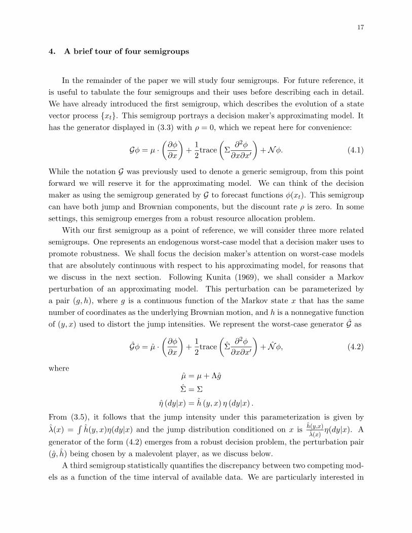
In the remainder of the paper we will study four semigroups. For future reference, itis useful to tabulate the four semigroups and their uses before describing each in detail.We have already introduced the first semigroup, which describes the evolution of a statevector process {xt}. This semigroup portrays a decision maker’s approximating model. Ithas the generator displayed in (3.3) with ρ = 0, which we repeat here for convenience:

Gφ = µ ·(

∂φ

∂x

)+

12trace

(Σ

∂2φ

∂x∂x′

)+Nφ. (4.1)

While the notation G was previously used to denote a generic semigroup, from this pointforward we will reserve it for the approximating model. We can think of the decisionmaker as using the semigroup generated by G to forecast functions φ(xt). This semigroupcan have both jump and Brownian components, but the discount rate ρ is zero. In somesettings, this semigroup emerges from a robust resource allocation problem.

With our first semigroup as a point of reference, we will consider three more relatedsemigroups. One represents an endogenous worst-case model that a decision maker uses topromote robustness. We shall focus the decision maker’s attention on worst-case modelsthat are absolutely continuous with respect to his approximating model, for reasons thatwe discuss in the next section. Following Kunita (1969), we shall consider a Markovperturbation of an approximating model. This perturbation can be parameterized bya pair (g, h), where g is a continuous function of the Markov state x that has the samenumber of coordinates as the underlying Brownian motion, and h is a nonnegative functionof (y, x) used to distort the jump intensities. We represent the worst-case generator G as

Gφ = µ ·(

∂φ

∂x

)+

12trace

(Σ

∂2φ

∂x∂x′

)+ Nφ, (4.2)

whereµ = µ + Λg

Σ = Σ

η (dy|x) = h (y, x) η (dy|x) .

From (3.5), it follows that the jump intensity under this parameterization is given by

λ(x) =∫

h(y, x)η(dy|x) and the jump distribution conditioned on x is h(y,x)

λ(x)η(dy|x). A

generator of the form (4.2) emerges from a robust decision problem, the perturbation pair(g, h) being chosen by a malevolent player, as we discuss below.

A third semigroup statistically quantifies the discrepancy between two competing mod-els as a function of the time interval of available data. We are particularly interested in

18

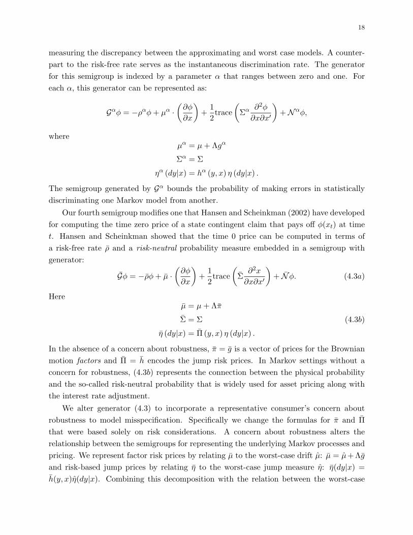
measuring the discrepancy between the approximating and worst case models. A counter-part to the risk-free rate serves as the instantaneous discrimination rate. The generatorfor this semigroup is indexed by a parameter α that ranges between zero and one. Foreach α, this generator can be represented as:

Gαφ = −ραφ + µα ·(

∂φ

∂x

)+

12trace

(Σα ∂2φ

∂x∂x′

)+Nαφ,

whereµα = µ + Λgα

Σα = Σ

ηα (dy|x) = hα (y, x) η (dy|x) .

The semigroup generated by Gα bounds the probability of making errors in statisticallydiscriminating one Markov model from another.

Our fourth semigroup modifies one that Hansen and Scheinkman (2002) have developedfor computing the time zero price of a state contingent claim that pays off φ(xt) at timet. Hansen and Scheinkman showed that the time 0 price can be computed in terms ofa risk-free rate ρ and a risk-neutral probability measure embedded in a semigroup withgenerator:

Gφ = −ρφ + µ ·(

∂φ

∂x

)+

12trace

(Σ

∂2x

∂x∂x′

)+ Nφ. (4.3a)

Hereµ = µ + Λπ

Σ = Σ

η (dy|x) = Π (y, x) η (dy|x) .

(4.3b)

In the absence of a concern about robustness, π = g is a vector of prices for the Brownianmotion factors and Π = h encodes the jump risk prices. In Markov settings without aconcern for robustness, (4.3b) represents the connection between the physical probabilityand the so-called risk-neutral probability that is widely used for asset pricing along withthe interest rate adjustment.

We alter generator (4.3) to incorporate a representative consumer’s concern aboutrobustness to model misspecification. Specifically we change the formulas for π and Πthat were based solely on risk considerations. A concern about robustness alters therelationship between the semigroups for representing the underlying Markov processes andpricing. We represent factor risk prices by relating µ to the worst-case drift µ: µ = µ+Λg

and risk-based jump prices by relating η to the worst-case jump measure η: η(dy|x) =h(y, x)η(dy|x). Combining this decomposition with the relation between the worst-case

19

semigroup generator rate drift jump

distortion dist. density

approximating model G 0 0 1

worst-case model G 0 g(x) h(y, x)

detection Gα ρα(x) gα(x) hα(y, x)

pricing G ρ(x) π(x) = g(x) + g(x) Π(x) = h(y, x)h(y, x)

Table 4.1: Parameterizations of the generators of four semigroups. The rate modifies the baselinegenerator by adding −ρφ to the generator for a test function φ. The drift distortion adds a termΛg · ∂φ

∂x to the baseline generator. The jump distortion density is used to build a replacement,h(y, x)η(dy|x), for the jump distribution η(dy|x) in the baseline generator.

and the approximating models gives the new vectors of pricing functions

π = g + g

Π = hh

where the pair (g, h) is used to depict the (constrained) worst-case model in (4.2). Laterwe will supply formulas for (ρ, g, h).

Table 4.1 summarizes our parameterization of these four semigroups. Subsequent sec-tions supply formulas for the entries in this table.

5. Statistical discrimination

We will use statistical discrimination to guide our thinking about how to calibratea concern about robustness. In designing a robust decision rule, we want our decisionmaker not to worry about alternative models that available time series data can disposeof easily. Therefore, before posing our robust decision problem, we study a stylized modelselection problem. Suppose that a decision-maker chooses between two models, whichwe will refer to as zero and one. Both are continuous-time Markov process models. Wedetermine how much time series data are needed to distinguish these models and thenuse the solution to this problem to motivate a measure of statistical discrepancy betweenmodels. This discrepancy measure will enter our adjustments to dynamic programmingthat are designed to accommodate model misspecification.

20

5.1. Measurement

We assume that there are direct measurements of the state vector {xt : 0 ≤ t ≤ N} andaim to discriminate between two Markov models: model zero and model one. We assignprior probabilities of one-half to each model. If we choose the model with the maximumposterior probability, two types of errors are possible, choosing model zero when one iscorrect and model one when model zero is correct. We weight these errors by the priorprobabilities and, following Chernoff (1952), study the error probabilities as the sampleinterval becomes large.

5.2. A semigroup formulation of bounds on error probabilities

We evade the difficult problem of precisely calculating error probabilities for nonlin-ear Markov processes and instead seek bounds on those error probabilities. To computethose bounds, we adapt Chernoff’s (1952) large deviation bounds to discriminate betweenMarkov processes. Large deviation tools apply here because the two types of error bothget small as the sample size increases. Let G0 denote the generator for Markov model zeroand G1 the generator for Markov model one. Both can be represented as in (3.6).

5.2.1. Discrimination in discrete time

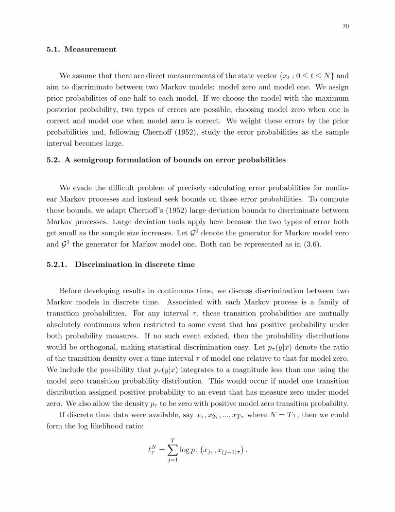
Before developing results in continuous time, we discuss discrimination between twoMarkov models in discrete time. Associated with each Markov process is a family oftransition probabilities. For any interval τ , these transition probabilities are mutuallyabsolutely continuous when restricted to some event that has positive probability underboth probability measures. If no such event existed, then the probability distributionswould be orthogonal, making statistical discrimination easy. Let pτ (y|x) denote the ratioof the transition density over a time interval τ of model one relative to that for model zero.We include the possibility that pτ (y|x) integrates to a magnitude less than one using themodel zero transition probability distribution. This would occur if model one transitiondistribution assigned positive probability to an event that has measure zero under modelzero. We also allow the density pτ to be zero with positive model zero transition probability.

If discrete time data were available, say xτ , x2τ , ..., xTτ where N = Tτ , then we couldform the log likelihood ratio:

`Nτ =

T∑

j=1

log pτ

(xjτ , x(j−1)τ

).

21

Model one is selected when

`Nτ > 0, (5.1)

and model zero is selected otherwise. The probability of making a classification error atdate zero conditioned on model zero is:

Pr{`Nτ > 0|x0 = x, model 0} = E

(1{`N

τ >0}|x0 = x, model 0)

.

It is convenient that the probability of making a classification error conditioned on modelone can also be computed as an expectation of a transformed random variable conditionedon model zero. Thus,

Pr{`Nτ < 0|x0 = x, model 1} = E

[1{`N

τ <0}|x0 = x, model 0]

= E[exp

(`Nτ

)1{`N

τ <0}|x0 = x, model 0].

The second equality follows because multiplication of the indicator function by the likeli-hood ratio exp

(`Nτ

)converts the conditioning model from one to zero. Combining these

two expressions, the average error is:

av error =12E

(min{exp

(`Nτ

), 1}

∣∣∣x0 = x, model 0)

. (5.2)

Because we compute expectations only under the model zero probability measure, fromnow on we leave implicit the conditioning on model zero.

0 0.2 0.4 0.6 0.8 1 1.2 1.4 1.6 1.8 20

0.2

0.4

0.6

0.8

1

1.2

1.4

1.6

1.8

2

exp(r)

min

(exp

(r),

1)

min(exp(r),1)

exp(α r)

Figure 5.1: Graph of min {exp(r), 1} and the dominating function exp(rα)for α = .5.

22

Instead of using formula (5.2) to compute the probability of making an error, we will usea convenient upper bound originally suggested by Chernoff (1952) and refined by Hellmanand Raviv (1970). To motivate the bound, note that the piecewise linear function min{s, 1}is dominated by the concave function sα for any 0 < α < 1 and that the two functionsagree at the kink point s = 1. The smooth dominating function gives rise to more tractablecomputations as we alter the amount of available data. Thus, setting log s = r = `N

τ andusing (5.2) gives the bound:

av error ≤ 12E

[exp

(α`N

τ

) ∣∣∣x0 = x]

(5.3)

where the right side is the moment-generating function for the log-likelihood ratio `Nτ (see

Fig. 5.1). Define an operator:

Kατ φ (x) = E

[exp (α`τ

τ ) φ (xτ )∣∣∣x0 = x

].

Then inequality (5.3) can be depicted as:

av error ≤ 12

(Kατ )T 1D (x)

where superscript T on the right side corresponds to sequential application of an operatorT times. This bound applies for any integer choice of T and any choice of α between zeroand one.23

When restricted to a function space C, we have the inequalities

|Kατ φ (x) | ≤ E

([exp (`τ

τ )]α |φ|

∣∣∣x0 = x)

≤ E[exp (`τ

τ ) |φ|1α

∣∣∣x0 = x]α

≤ ‖φ‖where the second inequality is an application of Jensen’s inequality. Thus Kα

τ is a contrac-tion on C.

Classification errors become less frequent as more data become available. One commonway to study the large sample behavior of classification error probabilities is to investigatethe limiting behavior of the operator (Kα

τ )T as T gets large. This amounts to studyinghow fast (Kα

τ )T contracts for large T and results in a large deviation characterization.Chernoff (1952) proposed such a characterization for i.i.d. data. Later it was extended toMarkov processes by various researchers. Formally, a large-deviation analysis gives riseto an asymptotic discrimination rate between models, when such a rate exists. We willinstead define a local discrimination rate that is formally applicable to continuous-timeprocesses. Before characterizing this rate, we consider the following example.

23 This bound covers the case in which model one density omits probability, and so equivalence betweenthe two measures is not needed for this bound to be informative.

23

5.2.2. Constant drift

Consider sampling a continuous multivariate Brownian motion with a constant drift. Letµ0, Σ0 and µ1, Σ1 be the drift vectors and constant diffusion matrices for models zero andone, respectively. Thus under model zero, xjτ − x(j−1)τ is normally distributed with meanτµ0 and covariance matrix τΣ0. Under an alternative model one, xjτ −x(j−1)τ is normallydistributed with mean τµ1 and covariance matrix τΣ1.

Suppose that Σ0 6= Σ1 and that the probability distributions implied by the two modelsare equivalent (i.e., mutually absolutely continuous). Equivalence will always be satisfiedwhen Σ0 and Σ1 are nonsingular but will also be satisfied when the degeneracy implied bythe covariance matrices coincides. It can be shown that

limτ↓0

Kατ 1D < 1

suggesting that a continuous-time limit will not result in a semigroup. Recall that asemigroup of operators must collapse to the identity when the elapsed interval becomes ar-bitrarily small. When the covariance matrices Σ0 and Σ1 differ, the detection-error boundremains positive even when the data interval becomes small. This reflects the fact thatwhile absolute continuity is preserved for each positive τ , it is known from Cameron andMartin (1947) that the probability distributions implied by the two limiting continuous-time Brownian motions will not be mutually absolutely continuous when the covariancematrices differ. Since diffusion matrices can be inferred from high frequency data, differ-ences in these matrices are easy to detect.24

Suppose that Σ0 = Σ1 = Σ. If µ0 − µ1 is not in the range of Σ, then the discrete-timetransition probabilities for the two models over an interval τ are not equivalent, makingthe two models easy to distinguish using data. If, however, µ0 − µ1 is in the range ofΣ, then the probability distributions are equivalent for any transition interval τ . Using acomplete-the-square argument, it can be shown that

Kατ φ (x) = exp (−τρα)

∫φ (y) Pα

τ (y − x) dy

where P τα is a normal distribution with mean τ(1 − α)µ0 + ταµ1 and covariance matrix

τΣ,

ρα =α (1− α)

2(µ0 − µ1

)′Σ−1

(µ0 − µ1

)(5.4)

24 The continuous time diffusion specification carries with it the implication that diffusion matrices can beinferred from high frequency data without knowledge of the drift. That data are discrete in practice tempersthe notion that the diffusion matrix can be inferred exactly. Nevertheless, estimating conditional means ismuch more difficult than estimating conditional covariances. Our continuous time formulation simplifies ouranalysis by focusing on the more challenging drift inference problem.

24

and Σ−1 is a generalized inverse when Σ is singular. It is now the case that

limτ↓0

Kατ 1D = 1.

The parameter ρα acts as a discount rate, since

Kατ 1D = exp (−τρα) .

The best probability bound (the largest ρα) is obtained by setting α = 1/2, and theresulting discount rate is referred to as Chernoff entropy. The continuous-time limit of thisexample is known to produce probability distributions that are absolutely continuous overany finite horizon (see Cameron and Martin, 1947).

For this example, the long-run and short-run discrimination rates coincide becauseρα is state independent. This equivalence emerges because the underlying processes haveindependent increments. For more general Markov processes, this will not be true and thecounterpart to the short-run rate will depend on the Markov state. The existence of a welldefined long-run rate requires special assumptions.

5.2.3. Continuous time

There is a semigroup probability bound analogous to (5.3) that helps to understandhow data are informative in discriminating between Markov process models. Suppose thatwe model two Markov processes as Feller semigroups. The generator of semigroup zero is

G0φ = µ0 ·(

∂φ

∂x

)+

12trace

(Σ

∂2φ

∂x∂x′

)+N 0φ

and the generator of semigroup one is

G1φ = µ1 ·(

∂φ

∂x

)+

12trace

(Σ

∂2φ

∂x∂x′

)+N 1φ

In specifying these two semigroups, we assume identical Σ’s. As in the example, thisassumption is needed to preserve absolute continuity. Moreover, we require that µ1 can berepresented as:

µ1 = Λg + µ0.

for some continuous function g of the Markov state, where we assume that the rank of Σis constant on the state space and can be factored as Σ = ΛΛ′ where Λ has full rank. Thisis equivalent to requiring that µ0 − µ1 is in the range of Σ.25

25 This can be seen by writing Λg = ΣΛ′(Λ′Λ)−1g.

25

In contrast to the example, however, both of the µ’s and Σ can depend on the Markovstate. Jump components are allowed for both processes. These two operators are restrictedto imply jump probabilities that are mutually absolutely continuous for at least somenondegenerate event. We let h(·, x) denote the density function of the jump distributionof N 1 with respect to the distribution of N 0. We assume that h(y, x)dη0(y|x) is finite forall x. Under absolute continuity we write:

N 1φ (x) =∫

h (y, x) [φ (y)− φ (x)] η0 (dy|x) .

Associated with these two Markov processes is a positive, contraction semigroup {Kαt :

t ≥ 0} for each α ∈ (0, 1) that can be used to bound the probability of classification errors:

av error ≤ 12

(KαN )1D (x) .

This semigroup has a generator Gα with the Feller form:

Gαφ = −ραφ + µα ·(

∂φ

∂x

)+

12trace

(Σ

∂2φ

∂x∂x′

)+Nαφ. (5.5)

The drift µα is formed by taking convex combinations of the drifts for the two models

µα = (1− α) µ0 + αµ1 = µ0 + αΛg;

the diffusion matrix Σ is the common diffusion matrix for the two models, and the jumpoperator Nα is given by:

Nαφ (x) =∫

[h (y, x)]α [φ (y)− φ (x)] η0 (dy|x)

Finally,

ρα (x) =(1− α) α

2g (x)′ g (x) +

∫ ((1− α) + αh (y, x)− [h (y, x)]α

)η0 (dy|x) . (5.6)

The term ρα is nonnegative and state dependent. The diffusion contribution

ραd (x) =

(1− α) α

2g (x)′ g (x)

is a positive semi-definite quadratic form and the jump contribution

ραn (x) =

∫ ((1− α) + αh (y, x)− [h (y, x)]α

)η0 (dy|x)

is positive because the tangent line to the concave function (h)α at h = 1 must lie abovethe function.

26

Theorem 5.1. (Newman, 1973 and Newman and Stuck, 1979). The generator of the

positive, contraction semigroup {Kαt : t ≥ 0} on C is given by (5.5).

Thus we can interpret the generator Gα that bounds the detection error probabilitiesas follows. Take model zero to be the baseline model or approximating model, and modelone to be some other competing model. We use 0 < α < 1 to build a mixed diffusion-jumpprocess from the pair (gα, hα) where gα .= αg and hα .= (h)α.

Use the notation Eα to depict the associated expectation operator. Then

av error ≤ 12Eα

[exp

(−

∫ N

0ρα (xt) dt

) ∣∣∣x0 = x

]. (5.7)

Of particular interest to us is formula (5.6) for ρα, which can be interpreted as a localstatistical discrimination rate between models. In the case of two diffusion processes, thismeasure is simply a state-dependent counterpart to formula (5.4) in our example. Thisrate is maximized by setting α = 1/2. When jump components are included, α = 1/2 willnot necessarily give the best rate. Theorem 5.1 describes the construction in the third rowof Table 4.1.

5.3. Digression on classical discrimination

For our later analysis, it will be useful to deduce a corresponding local measure ofconditional relative entropy, a limiting version of the local Chernoff measure ρα referred toabove. Conditional relative entropy plays a prominent role in large deviation theory andin classical statistical discrimination where it is sometimes used to study the decay in theso called type II error probabilities, holding fixed type I errors (Stein’s Lemma). Revertingfor the moment to discrete time, the relative entropy of model one with respect to modelzero is the expected log-likelihood ratio:

E(`Nτ

∣∣∣x0, model 1)

= E[`Nτ exp

(`Nτ

) ∣∣∣x0, model 0]

=d

dαE

[exp

(α`N

τ

) ∣∣∣x0 model 0] ∣∣∣

α=1,

(5.8)

where we have assumed that the model zero probability distribution is absolutely continu-ous with respect to the model A probability distribution. To evaluate entropy, the secondrelation differentiates the moment-generating function for the log-likelihood ratio. Fromthe same information inequality that justifies maximum likelihood estimation, it followsthat relative entropy is nonnegative.

27

We want a local version of entropy for continuous-time Markov models. As a counter-part to (5.8), we have the following local measure:

ε (x) = −dρα (x)dα

∣∣∣α=1

=g (x)′ g (x)

2+

∫[1− h (y, x) + h (y, x) log h (y, x)] η0 (dy|x)

(5.9)

The quadratic form g′g/2 comes from the diffusion contribution. Notice that it equals theChernoff measure ρα

d without the proportionality factor α(1− α). The term∫

[1− h (y, x) + h (y, x) log h (y, x)] η0 (dy|x)

measures the discrepancy in the jump intensities and distributions. It is positive by theconvexity of h log h in h. This formula presumes that the transition distribution for modelzero is absolutely continuous with respect to the transition distribution for model one.

5.4. Further discussion

The statistical decision problem posed above is in some ways too simple. It entails apairwise comparison of ex ante equally likely models and gives rise to a statistical measureof distance. The contenders are both Markov models, which greatly simplifies the boundson the probabilities of making a mistake when choosing between models. The implicitloss function that justifies model choice based on the maximal posterior probabilities issymmetric (e.g. see Chow, 1957). Finally, the detection problem compels the decision-maker to select a specific model after a fixed amount of data have been gathered.

Bounds like Chernoff’s can be obtained when there are more than two models andalso when the decision problem is extended to allow waiting for more data before makinga decision (e.g. see Hellman and Raviv, 1970 and Moscarini and Smith, 2002).26 Likeour problem, these generalizations can be posed as Bayesian problems with explicit lossfunctions and prior probabilities.

While the statistical decision problem posed here is by design too simple, we never-theless find it useful in bounding a reasonable taste for robustness. Rational expectationsinstructs agents and the model builder to eliminate misspecified models that are detectablefrom infinite histories of data. Chernoff entropy gives us one way to extend rational expec-tations by asking agents to entertain alternative models that are difficult to detect from

26 In particular, Moscarini and Smith (2002) consider Bayesian decision problems with a more general butfinite set of models and actions. Although they restrict their analysis to i.i.d. data, they obtain a morerefined characterization of the large sample consequences of accumulating information. Chernoff entropyremains a key ingredient in their analysis, however.

28

finite histories of data. When Chernoff entropy is small, it is challenging to choose betweencompeting models on purely statistical grounds.

6. Model misspecification and robust control

We now study the continuous-time robust resource allocation problem. In addition toan approximating model, this analysis will produce a constrained worst case model that isused as a device to make decisions robust.

6.1. Lyapunov equation under markov approximating model and a fixeddecision rule

Under a Markov approximating model with generator G and a fixed policy functioni(x), the decision maker’s value function is

V (x) =∫ ∞

0exp (−δt) E [U [xt, i (xt)] |x0 = x] dt.

The value function V satisfies the continuous-time Lyapunov equation:

δV (x) = U [x, i (x)] + GV (x) . (6.1)

Since V may not be bounded, we interpret G as the weak extension of the generator (3.6)defined using local martingales. The local martingale associated with this equation is:

Mt = V (xt)− V (x0)−∫ t

0(δV (xs)− U [xs, i (xs)]) ds.

As in (3.6), this generator can include diffusion and jump contributions.We will eventually be interested in optimizing over a control i, in which case the

generator G will depend explicitly on the control. For now we suppress that dependence.We refer to G as the approximating model; G can be modelled using the triple (µ, Σ, η) asin (3.6). The pair (µ, Σ) consists of the drift and diffusion coefficients while the conditionalmeasure η encodes both the jump intensity and the jump distribution.

We want to modify the Lyapunov equation (6.1) to incorporate a concern about modelmisspecification. We shall accomplish this by replacing G with another generator thatexpresses the decision maker’s precaution about the specification of G.

29

6.2. Entropy penalties

We now introduce perturbations to the decision maker’s approximating model that aredesigned to make finite horizon transition densities of the perturbed model be absolutelycontinuous with respect to those of the approximating model. We use a notion of absolutecontinuity that pertains only to finite intervals of time. In particular, imagine a Markovprocess evolving for a finite length of time. Our notion of absolute continuity restrictsprobabilities induced by the path {xτ : 0 ≤ τ ≤ t} for all finite t. See HSTW (2002) whodiscuss this notion as well as an infinite history version of absolute continuity. Kunita(1969) shows how to preserve both the Markov structure and absolute continuity.

As in Section 4 and following Kunita (1969), we shall consider a Markov perturbationthat can be parameterized by a pair (g, h), where g is a continuous function of the Markovstate x and has the same number of coordinates as the underlying Brownian motion, andh is a nonnegative function of (y, x) used to model the jump intensities. For the pair (g, h),the perturbed generator is portrayed using a drift µ+Λg, a diffusion matrix Σ, and a jumpmeasure h(y, x)η(dy|x). Thus the perturbed generator is given by

G (g, h) φ (x) = Gφ (x) + [Λ (x) g (x)] · ∂φ (x)∂x

+∫

[h (y, x)− 1] [φ (y)− φ (x)] η (dy|x) .

For this perturbed generator to necessarily be a Feller process would require that we imposeadditional restrictions on h. For analytical tractability we will only limit the perturbationsto have finite entropy. We will be compelled to show, however, that the perturbation usedto implement robustness does indeed generate a Markov process. This peturbation willbe constructed formally as the solution to a constrained minimization problem. In whatfollows, we continue to use the notation G to be the approximating model in place of themore tedious G(0, 1).

The conditional entropy measure [formula (5.9)] implied by this parameterization ofthe perturbed model is:

ε (g, h) (x) =g (x)′ g (x)

2+

∫[1− h (y, x) + h (y, x) log h (y, x)] η (dy|x)

where we now depict explicitly the dependence of ε on (g, h). Let ∆ denote the space ofall such pairs (g, h). Conditional relative entropy ε is convex in (g, h). It will be finite onlywhen

0 <

∫h (y, x) η (dy|x) < ∞.

When we introduce adjustments for model misspecification, we modify Lyapunov equa-tion (6.1) in the following way to penalize entropy

δV (x) = min(g,h)∈∆

U [x, i (x)] + θε (g, h) + G (g, h) V (x) ,

30

where θ > 0 is a penalty parameter. We are led to the following entropy penalty problem.

Problem AJ (V ) = inf

(g,h)∈∆θε (g, h) + G (g, h) V. (6.2)

Theorem 6.1. Suppose that (i) V is in C2 and (ii)∫

exp[−V (y)/θ]η(dy|x) < ∞ for all

x. The minimizer of Problem A is

g (x) = −1θΛ (x)′

∂V (x)∂x

h (y, x) = exp[−V (y) + V (x)

θ

].

(6.3a)

The optimized value of the criterion is:

J (V ) = −θG [

exp(−V

θ

)]

exp(−V

θ

) . (6.3b)

Finally, the implied measure of conditional relative entropy is:

ε∗ =V G [exp (−V/θ)]− G [V exp (−V/θ)]− θG [exp (−V/θ)]

θ exp (−V/θ). (6.3c)

Proof. The proof is in Appendix A.

In light of Theorem 6.1, our modified version of Lyapunov equation (6.1) is

δV (x) = min(g,h)∈∆

U [x, i (x)] + θε (g, h) + G (g, h) V (x)

= U [x, i (x)]− θG [

exp(−V

θ

)](x)

exp[−V (x)

θ

] .(6.4)

Replacing GV in the Lyapunov equation (6.1) by −θG[exp(−V

θ )]

exp(−Vθ )

can be interpreted as ad-

justing the continuation value for risk. For undiscounted problems, the connection betweenrisk-sensitivity and robustness is developed in a literature on risk-sensitive control (e.g. seeJames (1992) and Runolfsson (1994)). Hansen and Sargent’s (1995) recursive formulationof risk sensitivity accommodates discounting.

The connection is most evident when G = Gd so that x is a diffusion. Then

−θGd

[exp

(−Vθ

)]

exp(−V

θ

) = Gd (V )− 12θ

(∂V

∂x

)′Σ

(∂V

∂x

).

In this case, (6.4) is a partial differential equation. Notice that − 12θ scales ( ∂V

∂x )′Σ( ∂V∂x ),

the local variance of the value function process {V (xt)}. The interpretation of (6.4) under

31

risk sensitive preferences would be that the decision maker is concerned about both thelocal mean and the local variance of the continuation value process. The parameter θ isinversely related to the size of the risk adjustment. Larger values of θ assign a smallerconcern about risk. The term 1

θ is the so-called risk sensitivity parameter.Runolfsson (1994) deduced the δ = 0 (ergodic control) counterpart to (6.4) to obtain a

robust interpretation of risk sensitivity. Partial differential equation (6.4) is also a specialcase of the equation system that Duffie and Epstein (1992), Duffie and Lions (1992),and Schroder and Skiadas (1999) have analyzed for stochastic differential utility. Theyshowed that for diffusion models, the recursive utility generalization introduces a variancemultiplier that can be state dependent. The counterpart to this multiplier in our setup isstate independent and equal to the risk sensitivity parameter 1

θ .Though we are interested in the role of this variance multiplier in restraining entropy,

its mathematical connection to risk sensitivity and recursive utility lets us draw on a setof analytical results from those literatures.

Given a value function, Theorem 6.1 reports the formulas for the distortions (g, h) for aworst-case model used to enforce robustness. This model is Markov and depicted in termsof the value function. This theorem thus gives us a generator G and shows us how to fill outthe second row in Table 4.1. In fact, a separate argument is needed to show formally that Gdoes in fact generate a Feller process or more generally a Markov process. There are a hostof alternative sufficient conditions in the probability theory literature. Kunita (1969) givesone of the more general treatments of this problem and goes outside the realm of Fellersemigroups. Also, Ethier and Kurtz (1985, Chapter 8) give some sufficient conditions foroperators to generate Feller semigroups, including restrictions on the jump component Gn

of the operator.Using the Theorem 6.1 characterization of G, we can apply the results Theorem 5.1

to obtain the generator of a detection semigroup that measures the statistical discrepancybetween the baseline approximating model and the worst-case model.

We now consider some alternative, but closely related, ways to compute worst-casemodels used to enforce robustness.

32

6.3. An alternative entropy constraint

Epstein and Schneider (2001) criticize the formulation in Problem A by claiming thatit is dynamically inconsistent. Hansen and Sargent (2001) respond to that criticism bypointing out how the Markov perfect equilibrium automatically delivers all of the con-venient features for which one wants time consistency in the first place. Furthermore, aclosely related problem that avoids the complaints of Epstein and Schneider is:

Problem BJ∗ (V ) = inf

(g,h)∈∆,ε(g,h)≤εG (g, h) V, (6.5)

This problem has the same solution as that given by Problem A except that θ mustnow be chosen so that the relative entropy constraint is satisfied. That is, θ should bechosen so that ε(g, h) satisfies the constraint. The resulting θ will typically depend on x.The optimized objective must now be adjusted to remove the penalty:

J∗ (V ) = J (V )− θε∗ =V G [exp (−V/θ)]− G [V exp (−V/θ)]

exp (−V/θ),

which follows from (6.3c).While these formulas are a bit tedious, they simplify greatly when the approximating

model is a diffusion. Then θ satisfies

θ2 =12ε

(∂V (x)

∂x

)′Σ

(∂V (x)

∂x

).

This formulation embeds a version of the continuous-time preference order that Chen andEpstein (2001) proposed to capture uncertainty aversion. The diffusion version of thisrobust adjustment was also suggested in our earlier paper Anderson, Hansen and Sargent(1998).

33

6.4. Chernoff entropy

While Chernoff entropy is an essential ingredient of the theory of statistical discrimina-tion, in many cases it gives a less tractable formulation of an adjustment to the continuationvalue function to account for robustness than the relative entropy that we used in ProblemA.

Suppose that we replace ε(g, h) with the Chernoff measure:

(1− α) α

2g (x)′ g (x) +

∫ ((1− α) + αh− [h (y, x)]α

)η (dy|x)

for some α. The diffusion component:

(1− α) α

2g′g

is proportional to its counterpart in the conditional relative entropy measure. For instance,when α = 1/2, the Chernoff entropy scales the relative entropy by 1/4. Thus we can applyour previous calculations with θ or ε scaled appropriately.27

The jump component is∫ [

(1− α) + αh (y, x)− [h (y, x)]α]η (dy|x)

The solution to the counterpart to Problem (6.2) with Chernoff entropy is

h (y, x) =(

θα + V (y)− V (x)θα

) 1α−1

provided that θ is large enough to ensure that θα + V (y)− V (x) is positive. For some un-bounded value functions and state evolution specifications, there may not exist a constantθ that guarantees this positivity. On the other hand, a constraint version may be wellbehaved, since the θ could then depend on the state x. In what follows, we will limit ourattention to conditional relative entropy, while recognizing that this measure will coincidewith Chernoff entropy in the case of a diffusion, provided that the penalty parameter θ isappropriately adjusted.

27 Recall that bound (5.7) also uses a Markov evolution indexed by α. Introducing this into the Chernoffcounterpart to robust control problem (6.2) would require that we use a different probability law to evaluatethe discounted utility from the discounted entropy. This would induce an additional state variable to keeptrack of these separate expectations.

34

6.5. Enlarging the class of perturbations

In this paper we focus on the Markov formulation of robust control problems. In HSTWwe begin with a family of absolutely continuous perturbations to an approximating modelthat is a Markov diffusion. Absolute continuity over finite intervals puts a precise struc-ture on the perturbations, even when the Markov specification is not imposed on theseperturbations. As a consequence, HSTW follow James (1992) by considering path depen-dent specifications of the drift of the Brownian motion

∫ t0 gsds, where gs is constructed

as a general function of past x’s. Given the Markov structure of this control problem, itssolution can be represented as a time-invariant function of the state vector xt, which wedenote gt = g(xt).

6.6. Adding controls to the original state equation

We now allow the generator to depend on a control vector. Consider an approximatingMarkov control law of the form i(x) and let the generator associated with an approximatingmodel be G(i). For this generator, we introduce perturbation (g, h) as before. We write thecorresponding generator as G(g, h, i). To attain a robust decision rule, we use the Bellmanequation for a two-player Markov multiplier game:

δV = maxi

min(g,h)∈∆

U (x, i) + θε (g, h) + G (g, h, i) V. (6.6)

The Bellman equation for a corresponding constraint game is:

δV = maxi

min(g,h)∈∆(i),ε(g,h)≤ε

U (x, i) + G (g, h, i) V.

Sometimes infinite-horizon counterparts to terminal conditions must be imposed onthe solutions to these Bellman equations. Moreover, application of a Verification Theoremwill be needed to guarantee that the implied control laws are actually solve the requisiteMarkov game. Finally, these Bellman equations presume that the value function is twicecontinuously differentiable. It is well known that this differentiability does not alwaysobtain in problems in which the diffusion matrix can be made to be singular. In thesecircumstances there is typically a viscosity generalization to this Bellman equation with avery similar structure. (See Fleming and Soner (1991) for a development of the viscosityapproach to controlled Markov processes.)

35

7. Portfolio allocation

To put to work some of the results of Section 6, we now consider a robust portfolioproblem. In Section 8 we will use this problem to exhibit how asset prices can be deducedfrom the shadow prices of a robust resource allocation problem. We depart somewhat fromour previous notation and now let {xt : t ≥ 0} denote a state vector that is exogenous to theindividual investor. The investor influences the evolution of his wealth, which we denoteby wt. Thus the investor’s composite state at date t is (wt, xt). We consider first the casein which the exogenous component of the state vector evolves as a diffusion process. Laterwe let it be a jump process. Combining the diffusion and jump pieces is a straightforwardextension. We focus on the formulation with the entropy penalization used in Problem(6.2), but the constraint counterpart is similar.

7.1. Diffusion

An investor confronts asset markets that are driven by a Brownian motion. Under anapproximating model, the Brownian increment factors have date t prices given by π(xt)where xt evolves according to a diffusion:

dxt = µ (xt) dt + Λ (xt) dBt. (7.1)

Equivalently, this process has a generator Gd that is a second-order differential operatorwith drift µ and diffusion matrix Σ. A control vector bt entitles the investor to an in-stantaneous payoff bt · dBt with a price π(xt) · bt in terms of the consumption numeraire.This cost can be positive or negative. Adjusting for cost, the investment has payoff:−π(xt) · btdt + bt · dBt. There is also a market in a riskless security with an instantaneousrisk free rate ρ(x). The wealth dynamics are therefore

dwt = [wtρ (xt)− π (xt) · bt − ct] dt + bt · dBt, (7.2)

where ct is date t consumption. The control vector is i′ = (b′, c). Only consumption entersthe instantaneous utility function. By combining the evolution (7.1) and (7.2), we formthe evolution for a composite Markov process.

But the investor has doubts about this approximating model and wants a robust de-cision rule. Therefore he solves a version of game (6.6) with (7.1), (7.2) governing thedynamics of his composite state vector w, x. With only the diffusion component, theinvestor’s Bellman equation is

δV (w, x) = maxb

ming

U (c) + θε (g) + G (g, b, c) V

36

where G(g, b, c) is constructed using drift vector:[

µ (x) + Λ (x) gwρ (x)− π (x) · b− c + b · g

]

and diffusion matrix: [Λb′

][ Λ′ b ]

The choice of the worst case shock g satisfies the first-order condition:

θg + Vwb + Λ′Vx = 0 (7.3)

where Vw.= ∂V

∂w and similarly for Vx. Solving (7.3) for g gives a version of the solutiondepicted in Theorem 6.1. The resulting worst-case shock would depend on the controlvector b. In what follows we seek a solution that does not depend on b.

The first-order condition for consumption is:

Vw (w, x) = Uc (c) ,

and the first-order condition for the risk allocation vector b is:

−Vwπ + Vwwb + Λ′Vxw + Vwg = 0. (7.4)

In the limiting case in which the robustness penalty parameter is set to ∞, we obtain thefamiliar result that

b =πVw − Λ′Vxw

Vww

in which the portfolio allocation rule has a contribution from risk aversion measured by−Vw/wVww and a hedging demand contributed by the dynamics of the exogenous forcingprocess x.

Take the Markov perfect equilibrium of the relevant version of game (6.6). Providedthat Vww is negative, the same equilibrium decision rules prevail no matter whether oneplayer or the other chooses first, or whether they choose simultaneously. The first-orderconditions (7.3) and (7.4) are linear in b and g. Solving these two linear equations givesthe control laws for b and g as a function of the composite state (w, x):

b =θπVw − θΛ′Vxw + VwΛ′Vx

θVww − (Vw)2

g =VwΛ′Vxw − (Vw)2 π − VwwΛ′Vx

θVww − (Vw)2.

(7.5)

37

Notice how the robustness penalty adds terms to the numerator and denominator of theportfolio allocation rule. Of course, the value function V also changes when we introduceθ. Notice also that (7.5) give decision rules of the form

b = b (w, x)

g = g (w, x) ,(7.6)

and in particular how the worst case shock g feeds back on the consumer’s endogenousstate variable w. Permitting g to depend on w expands the kinds of misspecifications thatthe consumer considers.

7.1.1. Related formulations

So far we have studied portfolio choice in the case of a constant robustness parameterθ. Maenhout (2001) considers portfolio problems in which the robustness penalizationdepends on the continuation value. In his case the preference for robustness is designed sothat asset demands are not sensitive to wealth levels as is typical in constant θ formulations.Lei (2000) uses the instantaneous constraint formulation of robustness described in Section6.3 to investigate portfolio choice. His formulation also makes θ state dependent, since θ

now formally plays the role of a Lagrange multiplier that restricts conditional entropy atevery instant. Lei specifically considers the case of incomplete asset markets in which thecounterpart to b has a lower dimension than the Brownian motion.

7.1.2. Ex post Bayesian interpretation

The dependence of g on the endogenous state w can be unattractive from an ex postBayesian perspective. But there is a way to make this feature more acceptable. In partic-ular, we can use a representation like (2.5) to support an ex post Bayesian interpretationof the decision rule. We would form an exogenous state vector W that conforms to theMarkov perfect equilibrium of game (6.6):

dWt = µw (Wt, xt) dt + b (Wt, xt) · [g (Wt, xt) dt + dBt]

dxt = µ (xt) dt + Λ (xt) [g (Wt, xt) dt + dBt.](7.7)

If we confront a decision maker with this law of motion for the exogenous state vector andhave him not be concerned with robustness against misspecification of this law by settingθ = ∞, we pose an ordinary decision problem in which the decision maker has a uniquemodel. We initialize the exogenous state at W0 = w0. The optimal decision processesfor {(bt, ct)} (but not the control laws) will be identical for this decision problem and for

38

game (6.6) (see HSWT). This alternative problem gives a Bayesian rationale for the robustdecision procedure. Representation (7.7) is also valuable for representing prices that clearfinancial markets because it allows a recursive representations of security prices.

7.2. Jumps

Suppose now that the exogenous state vector {xt} evolves according to a Markov jumpprocess with jump measure η. To accommodate portfolio allocation, introduce the choiceof a function a that specifies how wealth changes when a jump takes place. Consider aninvestor who faces asset markets with date-state Arrow security prices given by Π(y, xt)where {xt} is an exogenous state vector with jump dynamics. In particular, a choice a

with instantaneous payoff a(y) if the state jumps to y has a price∫

Π(y, xt)a(y)η(dy|x) interms of the consumption numeraire. This cost can be positive or negative. When a jumpdoes not take place, wealth evolves according to

dwt =[ρ (xt−) wt− −

∫Π(y, xt−) a (y) η (dy|xt−)− ct−

]dt

where ρ(x) is the riskfree rate given state x and xt− = limτ↑t xτ . If the state x jumps to y

at date t, the new wealth is a(y). The Bellman equation for this problem is:

δV (w, x) = maxc,a

minh∈∆

U (c) + Vw (w, x)[ρ (x) wt −

∫Π(y, x) a (y) η (dy|x)− c

]

+ θ

∫[1− h (y, x) + h (y, x) log h (y, x)] η (dy|x)

+∫

h (y, x) (V [a (y) , y]− V (w, x)) η (dy|x)

The first-order condition for c is the same as for the diffusion case and equates Vw tothe marginal utility of consumption. The first-order condition for a requires

h (y, x) Vw [a (y) , y] = Vw (w, x)Π (y, x) ,

and the first-order condition for h requires

−θ log h (y, x) = V [a (y) , y]− V (w, x) .

Solving this second condition for h∗ gives the jump counterpart to the solution asserted inTheorem 6.1. Thus the robust a satisfies:

Vw [a (y) , y]Vw (w, x)

=Π (y, x)

exp(−V [a(y),y]+V (x)

θ

) .

39

In the limiting no-concern-about-robustness case θ = ∞, h is set to one. Since Vw isequated to the marginal utility for consumption, the first-order condition for a equatesthe marginal rate of substitution of consumption before and after the jump to the priceΠ(y, x). Introducing robustness scales the price by the jump distribution distortion.

In this portrayal, the worst case h depends on the endogenous state w, but it is againpossible to obtain an alternative representation of the probability distortion that wouldgive an ex post Bayesian justification for the decision process of a.

8. Pricing risky claims

By building on findings of Hansen and Scheinkman (2002), we now consider a fourthsemigroup that is to be used to price risky claims. We denote this semigroup by {Pt : t ≥ 0}where Ptφ assigns a price at date zero to a date t payoff φ(xt). That pricing should bedescribed by a semigroup follows from the Law of Iterated Values: a date 0 state-dateclaim φ(xt) can be replicated by first buying a claim Pτφ(xt−τ ) and then at time t − τ

buying a claim φ(xt). Like our other semigroups, this one has a generator, say G, that wewrite as in (3.3):

Gφ = −ρφ + µ ·(

∂φ

∂x

)+

12trace

(Σ

∂2φ

∂x∂x′

)+ Nφ

whereNφ =

∫[φ (y)− φ (x)] η (dy|x) .

The coefficient on the level term ρ is the instantaneous riskless yield. This contributionis needed to price locally riskless claims. Taken together, the remaining terms

µ ·(

∂φ

∂x

)+

12trace

(Σ

∂2φ

∂x∂x′

)+ Nφ

comprise the generator of the so called risk neutral probabilities. The risk neutral evolutionis Markov in this setting.

As discussed by Hansen and Scheinkman (2002), we should expect there to be a con-nection between the semigroup underlying the Markov process and the semigroup thatunderlies pricing. Like the semigroup for Markov processes, a pricing semigroup is pos-itive. Nonnegative functions of the Markov state are assigned nonnegative prices. Wecan thus relate the semigroups by importing the measure-theoretic notion of equivalence.Prices of contingent claims that pay off only in probability measure zero events should bezero. Conversely, when the price of a contingent claim is zero, the event associated with

40

that claim should occur only with measure zero, which states the principle of no-arbitrage.We can capture these properties by specifying that the generator G of the pricing semigroupsatisfies:

µ (x) = µ (x) + Λ (x) π (x)

Σ (x) = Σ (x)

η (x) = Π (y, x) η (dy|x)

(8.1)

where Π is strictly positive. Thus we construct equilibrium prices by producing a triple(ρ, π, Π). We now show how to do so both with and without a preference for robustness.

8.1. Marginal rate of substitution pricing

To compute prices, we follow Lucas (1978) and focus on the consumption side of themarket. While Lucas used an endowment economy, Brock (1982) showed that the essentialthing in Lucas’s analysis was not the pure endowment feature. Instead it was the idea ofpricing assets from marginal utilities evaluated at a candidate equilibrium consumptionprocess that can be computed prior to computing prices. As in Breeden (1979), we use acontinuous-time formulation that provides simplicity along some dimensions.28

8.2. Pricing without a concern for robustness

First consider the case in which the consumer has no concern about model misspec-ification. Proceeding in the spirit of Lucas (1978) and Brock (1982), we can constructmarket prices of risk from the shadow prices of a planning problem like that discussed inSection 2.1. For the reasons made clear by Lucas and Prescott (1971) and Prescott andMehra (1980), we solve a representative agent planning problem for a state process {xt},an associated control process {it} and a marginal utility of consumption processes {γt},respectively. We let G∗ denote the generator for the state vector process that emerges whenthe optimal controls from the resource allocation problem are imposed. Equivalently, G∗is the generator for the θ = ∞ robust control problem.

We construct a stochastic discount factor process by evaluating the marginal rate ofsubstitution at the proposed equilibrium consumption process:

mrst = exp (−δt)γ (xt)γ (x0)

where γ(x) denotes the marginal utility process for consumption as a function of the statex. Without a preference for robustness, the pricing semigroup satisfies

Ptφ (x) = E∗ [mrstφ (xt) |x0 = x] (8.2)28 This analysis differs from that of Breeden (1979) by its inclusion of jumps.

41

where the expectation operator E∗ is the one implied by G∗.Individuals solve a version of the portfolio problem described in Section 7 without

a concern for robustness. This supports the following depiction of the generator for theequilibrium pricing semigroup Pt:

ρ = −G∗γγ

+ δ

µ = µ∗ + Λ∗π = Λ∗Λ∗′∂ log γ

∂x

η (dy|x) = Π (y, x) η∗ (dy|x) =[γ (y)γ (x)

]η∗ (dy|x) .

(8.3)

These prices are the rational expectations risk prices familiar from previous research. Therisk-free rate is the subjective rate of discount reduced by the local mean of the equilibriummarginal utility process scaled by the marginal utility. The vector π of Brownian motionrisk prices are weights on the Brownian increment in the evolution of the marginal utilityof consumption, again scaled by the marginal utility. Finally the jump risk prices Π aregiven by the equilibrium marginal rate of substitution between consumption before andafter a jump.

8.3. Pricing under model misspecification

As in our previous analysis, let G denote the approximating model. This is the modelthat emerges by imposing the robust control law i but assumes there is no model mis-specification (g = 0 and h = 1). Let G denote the worst case model. This is the modelthat emerges as the Markov perfect solution to the two-player, zero-sum game. The ap-proximating or benchmark model G is arguably the counterpart to a rational expectationsmodel of the state evolution. This specification of beliefs, however, will not support theequilibrium prices (8.3) when G is used in place of G∗. Formula (8.3) will yield the equi-librium prices in an economy in which the individual agents use the worst-case generatorG instead of G∗ as their model of state evolution when making their decisions.

Let individual decision-makers use the worst-case model when designing their individ-ual portfolios as if it were the correct model to make risk assessments. This is differentfrom robust decision-making on the part of the individual agents. Rather than entertaininga family of models, the individuals presume or commit to the worst-case G as a model ofthe state vector {xt : t ≥ 0}. The pricing semigroup becomes

Ptφ (x) = E [mrstφ (xt) |x0 = x] (8.4)

where E denotes the mathematical expectation with respect to the distorted measuredescribed by the generator G. The generator for this pricing semigroup is parameterized

42

by

ρ = −Gγ

γ+ δ

µ = µ + Λg = µ + ΛΛ′∂ log γ

∂x

η (dy|x) = h (y, x) η (dy|x) =[γ (y)γ (x)

]η (dy|x)

. (8.5)

As in Subsection 8.2, ν(x) is the log of the marginal utility of consumption except it isevaluated at the solution of the robust planning problem. Individuals solve the portfolioproblem described in Section 7 using the worst-case model of the state {xt} with pricingfunctions π = g and Π = h specified relative to the worst-case model. Thus we refer to g

and h as risk prices because they are equilibrium prices that emerge from an economy inwhich individual agents use the worst-case model as if it were the correct model to assessrisk. The vector g contains the so-called factor risk prices associated with the vector ofBrownian motion increments. Similarly, h prices jump risk.

Comparison of (8.3) and (8.5) shows that the formulas for factor risk prices and the riskfree rate are identical except that we have used the distorted generator G in place of G∗.This comparison shows that we can use standard characterizations of asset pricing formulasif we simply replace the rational expectations generator with the distorted generator G.Appendix B justifies this decentralization.

8.4. Adjusting for belief distortion

With a preference for robustness, the approximating model G becomes central. It isthe centering point for perturbations. There is an alternative depiction of prices that usesthis model as a reference point. This gives a vehicle for defining model uncertainty pricesand for distinguishing between the contributions of risk and model uncertainty. The g andh from Subsection 8.3 give the risk components. We now use the discrepancy between Gand G to produce the model uncertainty prices.

To formulate model uncertainty prices, we now consider how prices can be representedunder the approximating model when the consumer has a preference for robustness. Wenow want to represent the pricing semigroup as

Ptφ (x) = E [(mrst) (mput) φ (xt) |x0 = x] (8.6)

where mpu is a multiplicative adjustment to the marginal rate of substitution that allowsus to evaluate the conditional expectation with respect to the approximating model ratherthan the distorted model. Instead of (8.3), to attain (8.6), we depict the drift and jump

43

distortion in the generator for the pricing semigroup as

µ = µ + Λg = µ + Λ(g + g)

η (dy|x) = h (y, x) η (dy|x) = h (y, x) h (y, x) η (dy|x) .

Changing expectation operators in depicting the pricing semigroup will not change theinstantaneous risk-free yield. Thus from Theorem 6.1 we have:

Theorem 8.1. Let V p be the value function for the robust resource allocation problem.

Suppose that (i) V p is in C2 and (ii)∫

exp[−V p(y)/θ]η(dy|x) < ∞ for all x. Moreover, γ

is assumed to be in the domain of the extended generator G. Then the equilibrium prices

are given by:

ρ = −Gγ

γ+ δ

π (x) = −1θΛ (x)′ V p

x (x) + Λ (x)′[γx (x)γ (x)

]= g (x) + g (x)

log Π (y, x) = −1θ

[V p (y)− V p (x)] + log γ (y)− log γ (x) = log h (y, x) + log h (y, x)

This theorem supplies the inputs into the last row of Table 4.1, and it follows directly fromthe relation between G and G given in Theorem 6.1 and from the risk prices of Subsection8.3.

We have already interpreted g and h as risk prices. Thus we view g = −1θΛ′V p

x as thecontribution to the Brownian exposure prices that comes from model uncertainty. Simi-larly, we think of h(y, x) = −1

θ exp[V p(y)−V p(x)] as the model uncertainty contribution tothe jump exposure prices. The additive decomposition for the Brownian motion exposureasserted in Theorem 8.1 was obtained previously as an approximation for linear-quadratic,Gaussian resource allocation problems by Hansen, Sargent, and Tallarini (1999). By study-ing continuous time diffusion models we have been able to sharpen their results and relaxthe linear-quadratic specification of constraints and preferences.

44

8.5. Decentralization and robust investors’ problems

We have already described how to support the robust resource allocation problem asone in which, in a decentralized economy, we endow an investor with beliefs G instead ofthe beliefs G associated with the approximating model, where G emerged from the robustplanning problem. Could these distorted beliefs G have been generated by having theconsumer solve a robust portfolio problem? We now given an affirmative answer to thisquestion.

Let V i(w, x) denote the value function of the investor in the robust portfolio allocationproblem in Section 7 where w is the financial wealth of the individual, and let gi(w, x)and hi(y, w, x) be the associated robust decision rules for the worst case distortions. Asbefore, we let V p(x) be the value function for the robust planning problem with associateddecision rules g(x), h(y, x) for the worst case distortions. The individuals and planner formworst-case models, but with different state variables. In this section and Appendix B weestablish the equivalence of these worst-case models in equilibrium.

Theorem 8.2.1. The prices from Theorem 8.1 support an equilibrium in which the consumers’ wealth

is an exact function of the state x that is exogenous to the consumer: w = ω(x).

2. The following equalities hold:

V p (x) = V i [ω (x) , x]

g (x) = gi [ω (x) , x]

h (y, x) = hi [y, ω (x) , x] .

Item 2 asserts that the same worst-case distortions emerge from the robust planning prob-lem and the robust portfolio problem at the equilibrium price process. We verify theseclaims in the remainder of this section and in Appendix B. We begin with the equilibriumwealth dynamics that emerge from the portfolio problem.

45

8.6. Wealth

Local prices emerge from the evolution of the intertemporal marginal rate of substitutionalong the solution of the robust planning problem. These local prices are encoded in thegenerator of the pricing semigroup. We can deduce values from local prices, includingwealth. For instance, let ψ(xt) be a dividend process for date t and let φ(x0) be the datezero value. Then

φ (x) =∫ ∞

0Ptψ (x) dt =

∫ ∞

0exp

(Gt)ψ (x) dt = −G−1ψ (x)

provided that

−Gφ = ψ

has a solution φ. While the domain of G might be quite limited, the domain of the inverseoften is considerably larger, including functions that are not necessarily smooth.

As with our application to value functions, we will seek values of unbounded functionsand necessarily work with the extended domain of the generator. Let {ξ(xt)} denotethe consumption process that is the outcome of the robust resource allocation problem.Corresponding to the function ξ used to represent consumption is a function ω used torepresent the equilibrium wealth as a function of the Markov process. In equilibriumwealth should be the risk-adjusted, present value of current and future consumption, andthus should solve

−Gω = ξ.

In a model with production, this wealth measure should also equal the value of the pro-ductive assets and other income sources owned by the consumer. In light of this pricingrelation, it follows that

Gdω (x) = ρ (x) ω (x)− ξ (x)− π (x) ·[Λ (x)′

∂ω (x)∂x

]−

∫[ω (y)− ω (x)] Π (y, x) η (dy|x) .

(8.7)where Gd is the diffusion component of the generator G.

This relation has the following interpretation. The local mean in equilibrium wealth hasan interest rate term ρω, a decrease induced by consumption ξ, and two price adjustments,one for the Brownian motion exposure with price vector π and one for the jump exposurewith price function Π. Given the candidate equilibrium consumption and pricing generator,equilibrium wealth as a function of the x is the solution to (8.7). This formula gives thealgorithm for constructing the function ω of the Theorem 8.2.

46

As justified in Appendix B, in equilibrium the processes for the individual decisionssatisfy:

at = ω (xt)

bt = Λ(xt)′ ∂ω

∂x(xt)

ct = ξ (xt) .

(8.8)

These are not the recursive decision rules for the individual control as a function of hisor her state (w, x). Instead these are equilibrium outcomes constructed after substitutingw = ω(x). Appendix B uses these as ingredients to establish Theorem 8.2.

8.7. More endogenous state variables

While we have considered a problem with a single endogenous state variable, financialwealth, there is a direct extension to the cases in which there are additional individualstate variables, such as household capital, that are often used to model durable goodsor habit persistence. In this circumstance, in a recursive formulation, individual decisionrules will depend on an individual version of this state. From the standpoint of individualchoice, this state variable will differ from its aggregate counterpart. The individual willpresume that he or she can influence the individual household capital stock while takingthe aggregate as given. In equilibrium the two will coincide.

8.8. Rational expectations reconsidered

In the distorted belief economy described in subsection 8.3, individual decision-makersadopt beliefs that may be distorted by state variables that are under the collective influenceof all decision-makers. For instance xt might include the physical capital stock, which canbe altered by aggregate investment. It turns out that the distortion can typically beisolated in the evolution of the exogenous (to the collective economy) component of thestate vector such as technology shocks or weather shocks. See HSTW for a discussionin the case of the diffusion specification. Thus the apparatus can be used to produce analternative model of the forcing processes such as technology shocks. Using the detectiontools discussed in Section 5, the alternative model could be required to be statisticallyclose to the baseline approximating model.

A rational expectations econometrician is endowed with only a finite history of datawhen considering alternative models of forcing processes. Consequently, such an econo-metrician looking to impose a statistically reasonable model of the forcing process couldimpose the law of motion implied by the approximating model, or might be persuaded

47

to specify the different and more complicated law of motion constructed from worst-casemodel. This latter construction could be done so that such an econometrician would havea difficult time discriminating between the two specifications of forcing processes. Usingeither specification, the econometrician could impose “rational expectations” by endowingindividual decision-makers with the same beliefs as in the specified law of motion for theforcing processes and computing equilibrium quantities and prices. By construction theequilibrium outcomes of the second specification would coincide the outcomes of the de-centralization of the robust resource allocation problem. While the forcing processes fromthe base line approximating model and the constructed alternative could be statisticallysimilar, implications for decisions and particularly prices could be quite different for thetwo models.

This construction of an equivalent rational expectations equilibrium based on theworst-case model works in a homogeneous consumer economy. Wealth heterogeneity, how-ever, would typically require ex post heterogeneity in beliefs not grounded in informationdifferences. Agents of different types might well have different worst case models of forcingprocesses. The tools described in this paper could ensure that the different perceptionsof the forcing processes were statistically similar, but there would still be implied hetero-geneity in beliefs.29

9. Entropy and market price of uncertainty

We now illustrate the relation between Chernoff entropy and the market price of modeluncertainty. Our examples use diffusion models. The price vector for the Brownian in-crements can be decomposed as: g + g. In the standard model without robustness, theconditional slope of a mean-standard deviation frontier is the absolute value of the factorrisk price vector: |g|. The counterpart including model uncertainty is: |g + g|. One state-ment of the equity-premium puzzle is that standard models imply a much smaller slopethan is found in the data. That is, standard models with reasonable risk aversion implya small value for g. This conclusion extends beyond the comparison of stocks and bonds.It is also apparent in equity return heterogeneity. See Hansen and Jagannathan (1991),Cochrane and Hansen (1992), and Cochrane (1997) for discussions.

In this section we explore the potential contribution from model uncertainty. In par-ticular, we investigate |g| for three example economies, and relate this to problems in

29 See Anderson (1998) for a discussion of resource allocation for a heterogenous-agent risk-sensitive econ-omy. The agents in this economy can also be viewed as either having a preference for robustness or het-erogenous beliefs.

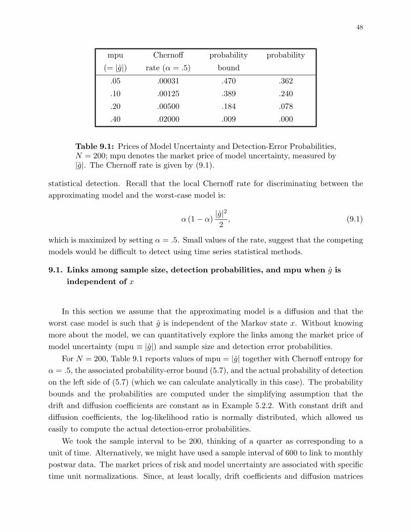
48

mpu Chernoff probability probability

(= |g|) rate (α = .5) bound

.05 .00031 .470 .362

.10 .00125 .389 .240

.20 .00500 .184 .078

.40 .02000 .009 .000

Table 9.1: Prices of Model Uncertainty and Detection-Error Probabilities,N = 200; mpu denotes the market price of model uncertainty, measured by|g|. The Chernoff rate is given by (9.1).

statistical detection. Recall that the local Chernoff rate for discriminating between theapproximating model and the worst-case model is:

α (1− α)|g|22

, (9.1)

which is maximized by setting α = .5. Small values of the rate, suggest that the competingmodels would be difficult to detect using time series statistical methods.

9.1. Links among sample size, detection probabilities, and mpu when g isindependent of x

In this section we assume that the approximating model is a diffusion and that theworst case model is such that g is independent of the Markov state x. Without knowingmore about the model, we can quantitatively explore the links among the market price ofmodel uncertainty (mpu ≡ |g|) and sample size and detection error probabilities.

For N = 200, Table 9.1 reports values of mpu = |g| together with Chernoff entropy forα = .5, the associated probability-error bound (5.7), and the actual probability of detectionon the left side of (5.7) (which we can calculate analytically in this case). The probabilitybounds and the probabilities are computed under the simplifying assumption that thedrift and diffusion coefficients are constant as in Example 5.2.2. With constant drift anddiffusion coefficients, the log-likelihood ratio is normally distributed, which allowed useasily to compute the actual detection-error probabilities.

We took the sample interval to be 200, thinking of a quarter as corresponding to aunit of time. Alternatively, we might have used a sample interval of 600 to link to monthlypostwar data. The market prices of risk and model uncertainty are associated with specifictime unit normalizations. Since, at least locally, drift coefficients and diffusion matrices

49

scale linearly with the time unit, the market prices of risk and model uncertainty scalewith the square root of the time unit.

The numbers in Table 9.1 indicate how market prices of uncertainty somewhat lessthan .2 are associated with misspecified models that are hard to detect. However, marketprices of uncertainty of .40 are associated with easily detectable alternative models. Thetables also reveal that although the probability bounds are weak, they display patternssimilar to those of the actual probabilities.

Empirical measures of the slope of the mean-standard deviation frontier are about.25 for quarterly data. Given the absence of volatility in aggregate consumption, riskconsiderations only explain a small component of the measured risk-return tradeoff usingaggregate data (Hansen-Jagannathan, 1991). In contrast, our calculations suggest thatconcerns about statistically small amounts of model misspecification could account for asubstantial component of the empirical measures.

9.2. Low frequency growth

Using a recursive utility specification, Bansal and Yaron (2000) study how low fre-quency components in consumption and/or dividends become encoded in risk premia.They emphasize how the frequency decomposition of risks matters. We will illustrate thishere using a simplified model. We shall reinterpret their risk premia as reflecting modeluncertainty.

Consider a pure endowment economy where the state x1t driving the consumptionendowment exp(x1t) is governed by the following process:

dx1t = (.0020 + .0554x2t) dt + .0048dBt

dx2t = −.0263x2tdt + .01dBt

. (9.2)

The logarithm of the consumption endowment has a constant growth rate .002 and a timevarying growth rate x2t; x2t has mean zero and is stationary but is highly temporallydependent. The inclusion of the x2t component alters the long run properties of consump-tion growth relative to an i.i.d. specification that would be obtained by zeroing out thecoefficient on x2t in the first equation.

We illustrate the persistence in consumption growth by depicting the impulse responseof log consumption to a Brownian motion shock in Fig. 9.1 and by displaying the spectraldensity function in Fig. 9.2. The low frequency component is a key feature in the analysisof Bansal and Yaron (2000). We calibrated the state evolution equation by embeddinga discrete-time consumption process that was fit by Bansal and Yaron in a continuous

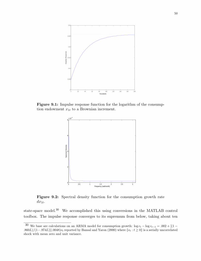
50

Time (Month)

Imp

uls

e R

esp

on

se

0 20 40 60 80 100 120 140 160 1800

0.005

0.01

0.015

0.02

0.025

0.03

Figure 9.1: Impulse response function for the logarithm of the consump-tion endowment x1t to a Brownian increment.

0 0.5 1 1.5 2 2.5 30

2

4

6

8x 10

−4

Frequency (rad/month)

Spectr

al D

ensity

Figure 9.2: Spectral density function for the consumption growth ratedx1t.

state-space model.30 We accomplished this using conversions in the MATLAB controltoolbox. The impulse response converges to its supremum from below, taking about ten

30 We base are calculations on an ARMA model for consumption growth: log ct − log ct−1 = .002 + [(1−.860L)/(1−.974L)](.0048)νt reported by Bansal and Yaron (2000) where {νt : t ≥ 0} is a serially uncorrelatedshock with mean zero and unit variance.

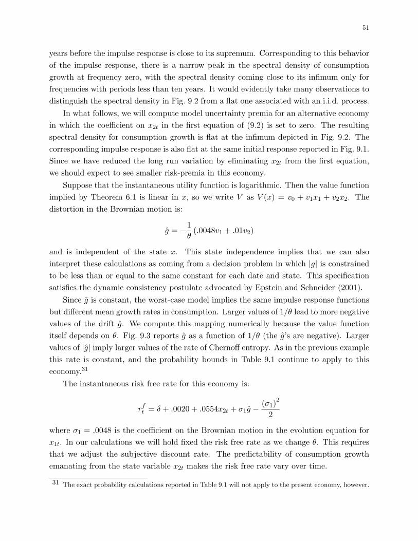
51

years before the impulse response is close to its supremum. Corresponding to this behaviorof the impulse response, there is a narrow peak in the spectral density of consumptiongrowth at frequency zero, with the spectral density coming close to its infimum only forfrequencies with periods less than ten years. It would evidently take many observations todistinguish the spectral density in Fig. 9.2 from a flat one associated with an i.i.d. process.

In what follows, we will compute model uncertainty premia for an alternative economyin which the coefficient on x2t in the first equation of (9.2) is set to zero. The resultingspectral density for consumption growth is flat at the infimum depicted in Fig. 9.2. Thecorresponding impulse response is also flat at the same initial response reported in Fig. 9.1.Since we have reduced the long run variation by eliminating x2t from the first equation,we should expect to see smaller risk-premia in this economy.

Suppose that the instantaneous utility function is logarithmic. Then the value functionimplied by Theorem 6.1 is linear in x, so we write V as V (x) = v0 + v1x1 + v2x2. Thedistortion in the Brownian motion is:

g = −1θ

(.0048v1 + .01v2)

and is independent of the state x. This state independence implies that we can alsointerpret these calculations as coming from a decision problem in which |g| is constrainedto be less than or equal to the same constant for each date and state. This specificationsatisfies the dynamic consistency postulate advocated by Epstein and Schneider (2001).

Since g is constant, the worst-case model implies the same impulse response functionsbut different mean growth rates in consumption. Larger values of 1/θ lead to more negativevalues of the drift g. We compute this mapping numerically because the value functionitself depends on θ. Fig. 9.3 reports g as a function of 1/θ (the g’s are negative). Largervalues of |g| imply larger values of the rate of Chernoff entropy. As in the previous examplethis rate is constant, and the probability bounds in Table 9.1 continue to apply to thiseconomy.31

The instantaneous risk free rate for this economy is:

rft = δ + .0020 + .0554x2t + σ1g − (σ1)

2

2

where σ1 = .0048 is the coefficient on the Brownian motion in the evolution equation forx1t. In our calculations we will hold fixed the risk free rate as we change θ. This requiresthat we adjust the subjective discount rate. The predictability of consumption growthemanating from the state variable x2t makes the risk free rate vary over time.

31 The exact probability calculations reported in Table 9.1 will not apply to the present economy, however.

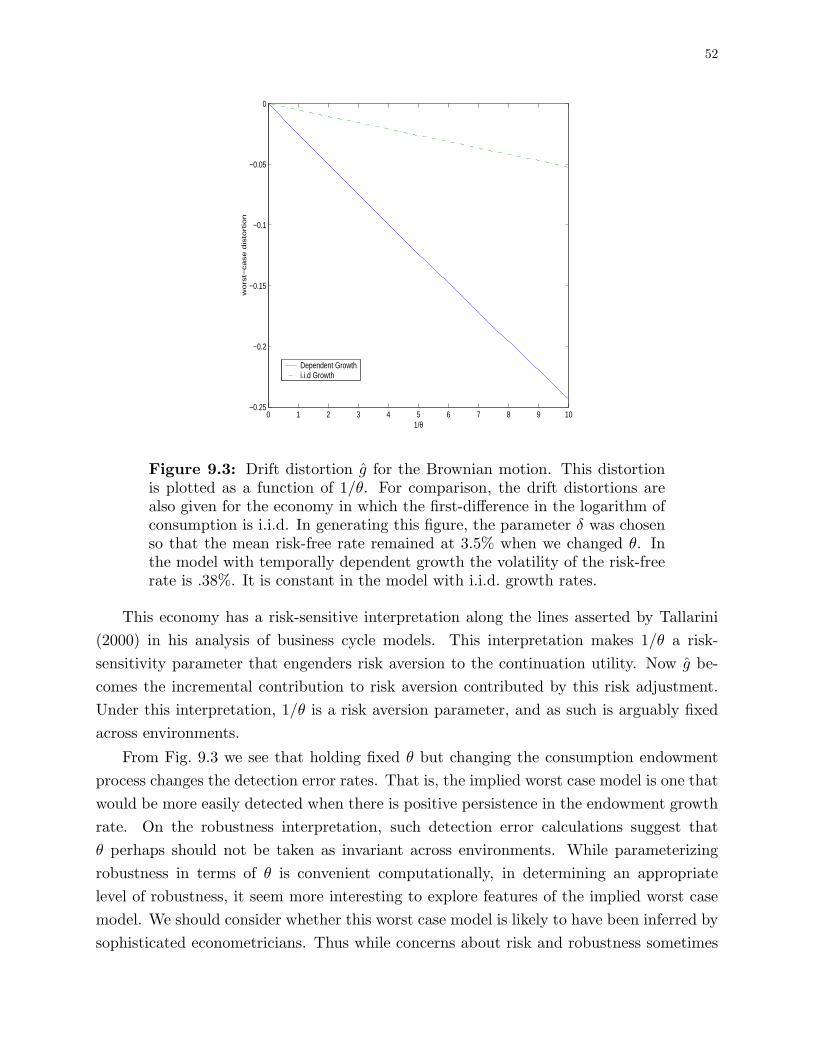
52

0 1 2 3 4 5 6 7 8 9 10−0.25

−0.2

−0.15

−0.1

−0.05

0

1/θ

wo

rst−

ca

se

dis

tort

ion

Dependent Growthi.i.d Growth

Figure 9.3: Drift distortion g for the Brownian motion. This distortionis plotted as a function of 1/θ. For comparison, the drift distortions arealso given for the economy in which the first-difference in the logarithm ofconsumption is i.i.d. In generating this figure, the parameter δ was chosenso that the mean risk-free rate remained at 3.5% when we changed θ. Inthe model with temporally dependent growth the volatility of the risk-freerate is .38%. It is constant in the model with i.i.d. growth rates.

This economy has a risk-sensitive interpretation along the lines asserted by Tallarini(2000) in his analysis of business cycle models. This interpretation makes 1/θ a risk-sensitivity parameter that engenders risk aversion to the continuation utility. Now g be-comes the incremental contribution to risk aversion contributed by this risk adjustment.Under this interpretation, 1/θ is a risk aversion parameter, and as such is arguably fixedacross environments.

From Fig. 9.3 we see that holding fixed θ but changing the consumption endowmentprocess changes the detection error rates. That is, the implied worst case model is one thatwould be more easily detected when there is positive persistence in the endowment growthrate. On the robustness interpretation, such detection error calculations suggest thatθ perhaps should not be taken as invariant across environments. While parameterizingrobustness in terms of θ is convenient computationally, in determining an appropriatelevel of robustness, it seem more interesting to explore features of the implied worst casemodel. We should consider whether this worst case model is likely to have been inferred bysophisticated econometricians. Thus while concerns about risk and robustness sometimes

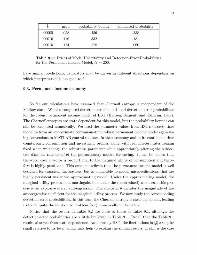
53

1θ mpu probability bound simulated probability

.00005 .058 .456 .338

.00010 .116 .332 .181

.00015 .174 .178 .060

Table 9.2: Prices of Model Uncertainty and Detection-Error Probabilitiesfor the Permanent Income Model, N = 200.

have similar predictions, calibrators may be driven in different directions depending onwhich interpretation is assigned to θ.

9.3. Permanent income economy

So far our calculations have assumed that Chernoff entropy is independent of theMarkov state. We also computed detection-error bounds and detection-error probabilitiesfor the robust permanent income model of HST (Hansen, Sargent, and Tallarini, 1999).The Chernoff entropies are state dependent for this model, but the probability bounds canstill be computed numerically. We used the parameter values from HST’s discrete-timemodel to form an approximate continuous-time robust permanent income model again us-ing conversions in MATLAB control toolbox. In their economy and in its continuous-timecounterpart, consumption and investment profiles along with real interest rates remainfixed when we change the robustness parameter while appropriately altering the subjec-tive discount rate to offset the precautionary motive for saving. It can be shown thatthe worst case g vector is proportional to the marginal utility of consumption and there-fore is highly persistent. This outcome reflects that the permanent income model is welldesigned for transient fluctuations, but is vulnerable to model misspecifications that arehighly persistent under the approximating model. Under the approximating model, themarginal utility process is a martingale, but under the (constrained) worst case this pro-cess is an explosive scalar autoregression. The choice of θ dictates the magnitude of theautoregressive coefficient for the marginal utility process. We now study the correspondingdetection-error probabilities. In this case, the Chernoff entropy is state dependent, leadingus to compute the solution to problem (5.7) numerically in Table 9.2.

Notice that the results in Table 9.2 are close to those of Table 9.1, although thedetection-error probabilities are a little bit lower in Table 9.1. Recall that the Table 9.1results abstract from state dependence. As shown by HST, the fluctuations in |g| are quitesmall relative to its level, which may help to explain the similar results. It still is the case

54

that statistical detection is difficult for market prices of uncertainty up to about say halfthat of the empirically measured magnitude.

Other model complications are also required to account fully for the steep slope of thefrontier. For instance, the model could be extended to include habit persistence or marketfrictions.32

10. Concluding remarks

In this paper we have applied tools from the mathematical theory of continuous-timeMarkov processes to explore the connections between model misspecification, risk, robust-ness, and model detection. We used these tools in conjunction with a decision theory thatcaptures the idea that the decision maker views his model as an approximation. An out-come of the decision making process is a penalized or constrained worst-case model thatis used to help make decision rules robust. In an equilibrium of a representative agenteconomy with such robust decision makers, the worst case model of a fictitious robustplanner must coincide with the worst case models of the representative private agents.These worst case models are endogenous outcomes of decision problems and give rise tomodel uncertainty premia in security markets. By adjusting constraints or penalties, theworst case models can be designed to be close in the sense that it is difficult statistically todiscriminate them from the original approximating model. These same penalties or con-straints limit the potency or magnitude of model uncertainty premia. Since mean returnsare hard to estimate, nontrivial departures in an approximating model are hard to detect.As a consequence, within limits imposed by statistical detection, there can still be sizablemodel uncertainty premia in security prices.

There is a less ambitious interpretation of our calculations. A rational expectationseconometrician is compelled to specify forcing processes, often without much guidanceexcept from statistics, for example, taking the form of a least squares estimate of anhistorical vector autoregression. The exploration of worst case models can be thoughtof as suggesting an alternative way of specifying forcing process dynamics that is inher-ently more pessimistic, but that leads to statistically similar processes. Not surprisingly,changing forcing processes can change equilibrium outcomes. More interesting is the fact

32 We find it fruitful to explore concern about model uncertainty because these other model modificationsare themselves only partially successful. To account fully for the market price of risk, Campbell and Cochrane(1999) adopt specifications with an arguably large amount of risk aversion during recessions. Constantinidesand Duffie (1996) accommodate fully the high market prices of risk by attributing empirically implausibleconsumption volatility to individual consumers (see Cochrane, 1997). Finally, Heaton and Lucas (1998)show that reasonable amounts of proportional transaction costs can only explain about half of the equitypremium puzzle.

55

that sometimes such subtle changes in perceived forcing processes can have quantitativelyimportant consequences on equilibrium prices.

Our altered decision problem introduces a robustness parameter that we restrict by us-ing detection probabilities. In assessing reasonable amounts of risk aversion in stochastic,general equilibrium models, it is common to explore preferences for hypothetical gam-bles in the manner of Pratt (1964). In assessing reasonable preferences for robustness,we propose using large sample detection probabilities for a hypothetical model selectionproblem. We envision a decision-maker as choosing to be robust to departures that arehard to detect statistically. Of course, using detection probabilities in this way is only oneway to discipline robustness. Exploration of other consequences of being robust, such asutility losses, would also be interesting. By borrowing ideas from robust control theorywe have produced an apparatus that shares the computational tractability of the standardrecursive theories of control and market equilibrium.

We see three important extensions to our current investigation. Like builders of ra-tional expectations models, we have side-stepped the issue of how decision-makers selectan approximating model. Following the literature on robust control, we envision this ap-proximating model to be analytically tractable, yet to be regarded by the decision makeras not providing a correct model of the evolution of the state vector. The misspecifica-tions we have in mind are small in a statistical sense but can otherwise be quite diverse.We have not formally modelled how agents learned the approximating model and whythey do not bother to learn about potentially complicated misspecifications of that model.Incorporating forms of learning would be an important extension of our work.33

The equilibrium calculations in our model currently exploit the representative agentparadigm in an essential way. Reinterpreting our calculations as applying to a multipleagent setting is straightforward in some circumstances (see Tallarini, 2000), but in general,even under complete security market structures, multiple agent versions of this environmentlook fundamentally different from their single-agent counterparts (see Anderson, 1998).Thus, the introduction of heterogeneous decision makers could lead to new insights aboutthe impact of concerns about robustness for market outcomes.

Finally, we obtain our most complete characterizations of decision problems and thedecentralized prices in the case of diffusion models. While the diffusion setup leads to some

33 One simple way to incorporate learning is to imitate the literature on adaptive learning models byhaving agents use a recursive learning algorithm to update information about a reference model. The usualpractice in adaptive control is to make decisions as if the estimated model would be the correct one fromthis point forward. Instead, the adaptive decision-maker could use the robust decision theory tools describedhere treating each estimated model as an approximation. Like adaptive control, this could be viewed as amodel of bounded rationality.

56

pedagogically useful simplifications, robustness considerations are likely to be particularlyimportant in environments with large shocks that occur infrequently, as in Poisson models.

57

References

Anderson, E. W. (1998), “Uncertainty and the Dynamics of Pareto Optimal Allocations,” University ofChicago Dissertation.

Anderson, E. W., L. P. Hansen and T. J. Sargent (1998), “Risk and Robustness in Equilibrium,” manuscript.

Bansal, R. and A. Yaron (2000), “Risks for the Long Run: A Potential Resolution of Asset Pricing Puzzles,”NBER Working Paper.

Blackwell, D. and M. Girshick (1954), Theory of Games and Statistical Decisions, Wiley: New York.

Bray, M. (1982), “Learning, Estimation, and the Stability of Rational Expectations,” Journal of EconomicTheory, 26:2, 318-39.

Breeden, D. T. (1979), “An Intertemporal Asset Pricing Model with Stochastic Consumption and InvestmentOpportunities,” Journal of Financial Economics 7, 265-296.

Brock, W. A. (1979), “An Integration of Stochastic Growth Theory and the Theory of Finance, Part I: TheGrowth Model,” General Equilibrium, Growth and Trade.

Brock, W. A, (1982), “Asset Pricing in a Production Economy,” In The Economics of Information andUncertainty, J. J. McCall, editor, Chicago: University of Chicago Press, for the National Bureau of EconomicResearch.

Brock, W. A. and M. J. P. Magill (1979), “Dynamics Under Uncertainty,” Econometrica 47, 843-868.

Brock, W. A. and L.J. Mirman (1972), “Optimal Growth Under Uncertainty: The Case of Discounting,”Journal of Economic Theory, 4:3, 479-513.

Cameron, H. R. and W.T. Martin (1947), “The Behavior of Measure and Measurability under Change ofScale in Wiener Space,” Bulletin of the American Mathematics Society, 53, 130-137.

Campbell, J. Y. and J. H. Cochrane (1999), “By Force of Habit: A Consumption-Based Explanation ofAggregate Stock Market Behavior,” Journal of Political Economy, 107:2, 205-251.

Chen, Z. and L. G. Epstein (2001), “Ambiguity, Risk and Asset Returns in Continuous Time,” manuscript.

Chernoff, H. (1952), “A Measure of Asymptotic Efficiency for Tests of a Hypothesis Based on the Sum ofObservations,” Annals of Mathematical Statistics, 23, 493-507.

Cho I.-K., Williams. N. and T.J. Sargent (2001), “Escaping Nash Inflation,” Review of Economic Studies,69:1, 1-40.

Chow, C. K. (1957), “An Optimum Character Recognition System Using Decision Functions,” Institute ofRadio Engineers (IRE) Transactions on Electronic Computers, 6, 247-254.

Cochrane, J. H. (1997), “Where is the Market Going? Uncertain Facts and Novel Theories,” Federal ReserveBank of Chicago Economic Perspectives, 21:6, 3-37.

Cochrane, J. H. and L. P. Hansen (1992), “Asset Pricing Lessons for Macroeconomics,” 1992 NBER Macroe-conomics Annual, O. Blanchard and S. Fischer (eds.), 1115-1165.

Constantinides, G. M. and D. Duffie (1996), “Asset Pricing with Heterogeneous Consumers,” Journal ofPolitical Economy, 104, 219-240.

Cox, J. C., J. E. Ingersoll, Jr. and S. A. Ross (1985), “An Intertemporal General Equilibrium Model ofAsset Prices,” Econometrica, 53, 363-384.

Dow, J. and S. R. C. Werlang (1994), “Learning under Knightian Uncertainty: The Law of Large Numbersfor Non-additive Probabilities, manuscript

Duffie, D. and L.G. Epstein (1992), “Stochastic Differential Utility,” Econometrica, 60:2, 353-394.

58

Duffie, D. and P.L. Lions (1992), “PDE Solutions of Stochastic Differential Utility,” Journal of MathematicalEconomics, 21, 577-606.

Duffie, D. and C. Skiadas (1994), “Continuous-Time Security Pricing: A Utility Gradient Approach,” Journalof Mathematical Economics, 23, 107-131.

Dupuis, P. and R. S. Ellis (1997), A Weak Convergence Approach to the Theory of Large Deviations, NewYork: John Wiley and Sons.

Dynkin, E. B. (1956), “Markov Processes and Semigroups of Operators,” Theory of Probability and itsApplications 1, 22-33.

Elliot, R. J., L. Aggoun, and J. B. Moore (1995), Hidden Markov Models: Estimation and Control, Springer:New York.

Ellsberg, D. (1961), “Risk, Ambiguity, and the Savage Axions,” Quarterly Journal of Economics, 75:4,643-669.

Epstein, L. G. and M. Schneider (2001), “Recursive Multiple Priors,” manuscript.

Epstein, L.G. and T. Wang (1994), “Intertemporal Asset Pricing Under Knightian Uncertainty,” Economet-rica, 62:3, 283-322.

Epstein, L.G. and S.E. Zin (1989), “Substitution, Risk Aversion and the Temporal Behavior of Consumptionand Asset Returns: A Theoretical Framework,” Econometrica, 57:4, 937-969.

Evans, G. W. and S. Honkapohja (2001), Learning and expectations in macroeconomics, Princeton: PrincetonUniversity Press.

Fleming, W. H. and H. M. Soner (1991), Controlled Markov Processes and Viscosity Solutions, New York:Springer-Verlag

Fudenberg, D. and D. K. Levine (1998), The Theory of Learning in Games, Cambridge: MIT Press.

Hansen, L.P. and R. Jagannathan (1991), “Implications of Security Market Data for Models of DynamicEconomies,” Journal of Political Economy, 99:2, 225-262.

Hansen, L.P. and T.J. Sargent (1993), “Seasonality and Approximation Errors in Rational ExpectationsModels,” Journal of Political Economy, 55, 21-55

Hansen, L.P. and T.J. Sargent (1995), “Discounted Linear Exponential Quadratic Gaussian Control,” IEEETransactions on Automatic Control, 40:5, 968-971.

Hansen, L.P. and T.J. Sargent (2001), “Time Inconsistency of Robust Control?”, manuscript.

Hansen, L.P. and T.J. Sargent (2004), Robust Control and Economic Model Uncertainty, Princeton: Prince-ton University Press.

Hansen, L.P., T.J. Sargent and T.D. Tallarini, Jr. (1999), “Robust Permanent Income and Pricing,” Reviewof Economic Studies, 66, 873-907.

Hansen, L.P., T.J. Sargent, G.A. Turmuhambetova, and N. Williams (2002), “Robustness and UncertaintyAversion,” manuscript.

Hansen, L.P., T.J. Sargent, and N.E. Wang (2002), “Robust Permanent Income and Pricing with Filtering,”Macroeconomic Dynamics, 6, February, pp. 40–84.

Hansen, L.P. and J. Scheinkman (2002), “Semigroup Pricing,” manuscript.

Heaton, J. C. and D. J. Lucas (1996), “Evaluating the Effects of Incomplete Markets on Risk Sharing andAsset Pricing,” Journal of Political Economy, 104, 443-487.

Hellman, M. E. and J. Raviv, (1970), “Probability Error, Equivocation, and the Chernoff Bound,” IEEETransactions on Information Theory, 16, 368-372.

59

James, M.R. (1992), “Asymptotic Analysis of Nonlinear Stochastic Risk-Sensitive Control and DifferentialGames,” Mathematics of Control, Signals, and Systems, 5, 401-417.

Jorgenson, D.W. (1967), “Discussion,” The American Economic Review, 57:2, Papers and Proceedings,557-559.

Knight, F.H. (1921), Risk, Uncertainty and Profit, Boston: Houghton Mifflin.

Kreps, D. (1998), “Anticipated Utility and Dynamic Choice,” Kalai, E. and Kamien, M. I. ( eds.), Frontiers ofresearch in economic theory: The Nancy L. Schwartz Memorial Lectures, Econometric Society Monographs,no. 29, Cambridge: Cambridge University Press, 242-74.

Kunita (1969), H. “Absolute Continuity of Markov Processes and Generators,” Nagoya Math. Journal, 36,pages 1 -26

Kurz, M. (1997), Endogenous Economic Fluctuations: Studies in the Theory of Rational Beliefs, New York:Springer.

Lei, C. I. (2000), Why Don’t Investors have Large Positions in Stocks? A Robustness Perspective, unpublishedPh.D. Dissertation, University of Chicago.

Lucas, R.E., Jr (1976), “Econometric Policy Evaluation: A Critique,” Journal of Monetary Economics, 1:2,19-46.

Lucas, R. E., Jr. (1978), “Asset Prices in an Exchange Economy,” Econometrica, 46:6, 1429-1445.

Lucas, R.E., Jr. and E.C. Prescott (1971), “Investment under Uncertainty,” Econometrica, 39:5, 659-681.

Maenhout, P. (2001), “Robust Portfolio Rules, Hedging and Asset Pricing”, manuscript, INSEAD.

Merton, R. (1973), “An Intertemporal Capital Asset Pricing Model,” Econometrica, 41, 867-888.

Moscarini, G. and L. Smith (2002), “The Law of Large Demand for Information,” manuscript, forthcomingin Econometrica.

Newman. C. M. (1973), “The orthogonality of independent increment processes,” in Topics in ProbabilityTheory, D.W. Stroock and S.R.S. Varadhan (eds.), 93-111, Courant Institute of Mathematical Sciences,N.Y.U.

Newman, C. M. and B. W. Stuck (1979), “Chernoff Bounds for Discriminating Between Two Markov Pro-cesses,” Stochastics, 2, 139-153.

Petersen, I.R., M. R. James and P. Dupuis (2000), “Minimax Optimal Control of Stochastic UncertainSystems with Relative Entropy Constraints,” IEEE Transactions on Automatic Control, 45, 398-412.

Pratt, J. W. (1964), “Risk Aversion in the Small and Large,” Econometrica, 32:1-2, 122-136.

Prescott, E.C. and R. Mehra (1980), “Recursive Competitive Equilibrium: The Case of Homogeneous House-holds,” Econometrica, 48, 1365-1379.

Revuz D. and M. Yor (1994), Continuous martingales and Brownian motion, 2nd ed., New York: SpringerVerlag.

Runolfsson, T. (1994), “The Equivalence between Infinite-horizon Optimal Control of Stochastic Systemswith Exponential-of-integral Performance Index and Stochastic Differential Games,” IEEE Transactions onAutomatic Control, 39, 1551-1563.

Schroder, M. and C. Skiadas (1999), “Optimal Consumption and Portfolio Selection with Stochastic Differ-ential Utility,” Journal of Economic Theory, 89, 68-126.

Sims, C. A. (1993), “Rational Expectations Modelling with Seasonally Adjusted Data,” Journal of Econo-metrics, 55.

Tallarini, Jr., T.D. (2000), “Risk-Sensitive Real Business Cycles,” Journal of Monetary Economics, 45:3,507-32.

60

A. Entropy Solution

This appendix contains the proof of Theorem 6.1.

Proof. To verify the conjectured solution, first note that the objective is additively separable in g and h.Moreover the objective for the quadratic portion in g is:

θg′g2

+ g′Λ′∂V

∂x. (A.1)

Minimizing this component of the objective by choice of g verifies the conjectured solution. The diffusioncontribution to the optimized objective including (A.1) is:

Gd (V )− 12θ

(∂V

∂x

)′Σ

(∂V

∂x

)= −θ

Gd [exp (−V/θ)]exp (−V/θ)

where we are using the additive decomposition: G = Gd + Gn. Very similar reasoning justifies the diffusioncontribution to entropy formula (6.3c).

Consider next the component of the objective that depends on h:

θ

∫[1− h (y, x) + h (y, x) log h (y, x)] η (dy|x) +

∫h (y, x) [V (y)− V (x)] η (dy|x) (A.2)

To verify34 that this objective is minimized by h, first use the fact that 1− h + h log h is convex and hencedominates the tangent line at h. Thus

1− h + h log h ≥ 1− h + h log h + log h(h− h

).

This inequality continues to hold when we multiply by θ and integrate with respect to η(dy|x). Thus

θε (h) (x)− θ

∫h (y, x) log h (y, x) η (dy|x) ≥ θε

(h)

(x)− θ

∫h (y, x) log h (y, x) η (dy|x) .

Substituting for log[h(y, x)] shows that h minimizes (A.2), and the resulting objective is:

θ

∫ [1− h (y, x)

]η (dy|x) = −θ

Gn exp (−V/θ)exp (−V/θ)

,

which establishes the jump contribution to (6.3b). Very similar reasoning justifies the jump contribution to(6.3c)

34 In the special case in which the number of states is finite and the probability of jumping to any of thesestates is strictly positive, a direct proof that h is the minimizer is available. Abusing notation somewhat, letη (yi|x) > 0 denote the probability that the state jumps to its ith possible value, yi given that the currentstate is x. We can write the component of the objective that depends upon h (which is equivalent to equation(A.2) in this special case) as

θ +n∑

i=1

η (yi|x) [−θh (yi, x) + θh (yi, x) log h (yi, x) + h (yi, x)V (yi)− h (yi, x)V (x)] .

Differentiating this expression with respect to h (yi, x) yields η (yi|x) [θ log h (yi, x) + V (yi)− V (x)]. Settingthis derivative to zero and solving for h (yi, x) yields h (yi, x) = exp[V (x)−V (yi)

θ ], which is the formula for hgiven in the text.

61

B. Decentralization

In this appendix we consider two decentralizations and the proofs of Theorem 8.1 and Theorem 8.2. Thefirst decentralization assumes that the individual is committed to the worst-case model. The decentralizationis similar to that of Lucas (1978) and Breeden (1979). The second has the individual choose worst-casemodels to support robust decisions. In both cases, we adopt a recursive formulation rather than a date zeroformulation with state and date contingent claims. See Duffie and Skiadis (1993) and Hansen, Sargent andTallarani (1999) for examples in which a date zero formulation is made tractable through the computationof appropriate subgradients for consumers. We use the recursive formulation here to be consistent withthe remainder of our paper. This seems particularly appropriate because our worst-case models depend oncontinuation values, and these values will need to be computed as part of the equilibrium. On the otherhand, we will be casual in our treatment of terminal wealth. Typically a Verification Theorem will need toemployed to justify formally the solution to individuals decision problem.

In what follows we are casual (or bold) in assuming the existence of derivatives.

B.1. Risk decentralization

Let V (w, x) denote the individual investor’s value function. We seek an equilibrium in which theendogenous state wt = ω(xt) and the corresponding costate, γt = γ(xt), which is equivalently the marginalutility of consumption and the marginal utility of wealth. The function ω solves:

Gω = −ξ, (B.1)

and the function γ is given by:γ = Uc ◦ ξ.

Notice that from the construction of ρ,δγ = ργ + Gγ. (B.2)

We will verify that (B.1) gives rise to the state equation for the individual control problem evaluated at thecandidate equilibrium prices. This state equation is degenerate in the sense that financial wealth wt = ω(xt)is an exact function of the state xt. Equation (B.2) gives rise to the corresponding co-state equation, wherethe costate mut = γ(xt) is also an exact function of the state vector xt.

Before investigating the state and costate equations, we consider the optimal controls at the candidateprices. We seek a solution in which a(y) = ω(y), b = Λ′ωx and c = ξ. These are not the individual controllaws, which also depend on financial wealth w. Instead these are the outcomes of these control laws whenw = ω(x). The candidate risk prices are π = g = Λξx and Π(y, x) = h(y, x) = Uc◦ξ(y)

Uc◦ξ(x) and are specified

relative to the worst-case G model.The first-order conditions for consumption at the candidate equilibrium are:

Vw [ω (x) , x] = Uc [ξ (x)] . (B.3)

Differentiating this with respect to x gives:

Vwwωx + Vwx = Uccξx.

Multiplying this relation by Λ′ gives

VwwΛ′ωx + Λ′Vwx = UccΛ′ξx,

or equivalentlyVww b + Λ′Vwx = Vwπ.

This equation is the first-order condition for the choice b in the absence of robustness. (See (7.4) with g setto zero.)

62

We now turn to the jump risk. The function a specifies how wealth changes when a jump takes place.The first-order condition for a requires:

Vw [a (y) , y]Vw [ω (x) , x]

= Π (y, x) =Uc [ξ (y)]Uc [ξ (x)]

.

In light of (B.3), this will be satisfied by setting a = ω.In equilibrium we also require that ω must evolve in a way that respects individual budget balance at

the equilibrium prices. This gives rise to an operator counterpart to a state equation for the endogenousfinancial wealth constraint. Since ω satisfies (B.1),

Gdω (x) = ρ (x) ω (x)− π (x) · b (x)−∫

Π (y, x) [a (y)− ω (x)] η (dy|x)− c (x) .

The local mean in ω is equal to the instantaneous rate of return to financial wealth adjusted for exposureto both the Brownian motion and jump risk and net of instantaneous consumption. The right-hand side ofthis equation is a flow budget constraint evaluated at the candidate equilibrium.

The equilibrium interest rate ρ is set to satisfy a co-state equation. The costate γt is given by

γt = Vw [ω (xt) , xt] = Uc [ξ (xt)].= γ (xt)

where the second equality is the first-order condition for consumption. The Envelope Theorem gives aforward-looking formula for Vw obtained by differentiating the Bellman equation with respect to w. Theoperator counterpart implies that

δVw [ω (x) , x] = ρ (x)Vw [ω (x) , x] + GVw [ω (x) , x] .

This formula is satisfied because (B.2) is satisfied and γ = Vw.

B.2. Robustness decentralization

We now suppose that the individual consumer has preferences that support a concern about robustness.As in the text we distinguish between two value functions: V i is the individual’s value function and V p

is the value function for the planner. We aim to support the same consumption and wealth specificationsas well as the control processes: a(y) = ω(y), b = Λ′ωx and c = ξ, but we give the decentralized prices adifferent interpretation. The formulas for π and Π differ because the price adjustments are now relative tothe baseline G model instead of the worst-case G. As a consequence, our candidate prices are π = g + g andΠ = hh.

We want the value functions to be related via:

V i [ω (x) , x] = V p (x) . (B.4)

These value functions are used to give two depictions of worst-case shocks, one for the individualdecision-maker and one for the fictitious robust planner. Differentiating (B.4) with respect to x gives:

V iwωx + V i

x = V px

Premultiplying by Λ′ and adding θg gives:

θg + V iw (Λ′ωx) + Λ′V i

x = θg + ΛV px

The right-hand side is zero when g is the worst-case drift distortion from the robust resource allocationproblem. The left-hand side is the first-order condition (7.3) for the worst case drift distortion for theindividual problem provided that

Λ′ωx = b,

63

which is the candidate solution. Thus a common formula links the two-worst case g’s, and this formula isinterpretable as the first-order condition for g from both individual optimization and planner optimization.

The value function equivalence (B.4) is sufficient to verify the equivalence of the worst-case h’s for therobust planner and the robust individual decision maker.

To verify the remaining controls, we imitate our previous argument based on: V iw = Uc to conclude that

V iwwΛ′ωx + Λ′V i

wx = UccΛ′ξx,

or equivalentlyV i

ww b + Λ′V iwx + V i

wg = V iwπ,

which is the first-order condition (7.4). The first-order conditions for the choice of a are:

exp(−V i [a (y) , y] + V i (w, x)

θ

)V i

w [a (y) , y] = V iw (w, x) Π (y, x) .

Thus from relation (B.4), we have that

exp(−V p (y) + V p (x)

θ

)V i

w [a (y) , y] = V iw (w, x) Π (y, x) ,

orV i

w [a (y) , y] = V iw (w, x) h (y, x) .

This equality follows from the first-order condition for consumption Vw = Uc because h is the marginal rateof substitution between the pre-jump and post-jump consumption rates.

The arguments for the state and costate equations proceed as in our risk decentralization.Finally, to establish (B.4) we know that V p satisfies the Lyapunov equation for the robust resource

allocation problem and V i for the robust individual decision problem. These Lyapunov equations are theones for the objective function of the two-player games but are evaluated at the optimized control processes.To verify (B.4), we show that the Lyapunov for the individual problem evaluated at w = ω(x) is the Lyapunovequation for the robust planner’s problem. The individual Lyapunov equation is,

δV i [ω (x) , x] = U [c (x)] + V iw [ω (x) , x]

[Gdω (x)

]+ µ (x) · V i

x [ω (x) , x]

+b (x)′ b (x)

2+ b (x)′ Λ (x) V i

x [ω (x) , x]

+12trace

(Σ(x)V i

xx [ω (x) , x])

+∫ (

V i [a (y) , y]− V i [ω (x) , x])η (dy|x) + θε

(g, h

)(x)

where we have substituted in the worst-case model. Substituting for the optimized control process (a, b, c),and using (B.4) yields the Lyapunov equation:

δV p (x) = U [ξ (x)] + GV p (x) + θε(g, h

)(x) .