a profit model for spread trading with an application to...

A profit model for spread trading with an application to energy futures

by Takashi Kanamura, Svetlozar T. Rachev, Frank J. Fabozzi

No. 27 | MAY 2011

WORKING PAPER SERIES IN ECONOMICS

KIT – University of the State of Baden-Wuerttemberg andNational Laboratory of the Helmholtz Association econpapers.wiwi.kit.edu

Impressum

Karlsruher Institut für Technologie (KIT)

Fakultät für Wirtschaftswissenschaften

Institut für Wirtschaftspolitik und Wirtschaftsforschung (IWW)

Institut für Wirtschaftstheorie und Statistik (ETS)

Schlossbezirk 12

76131 Karlsruhe

KIT – Universität des Landes Baden-Württemberg und

nationales Forschungszentrum in der Helmholtz-Gemeinschaft

Working Paper Series in Economics

No. 27, May 2011

ISSN 2190-9806

econpapers.wiwi.kit.edu

A Profit Model for Spread Trading with an Application

to Energy Futures

Takashi Kanamura

J-POWER

Svetlozar T. Rachev∗

Chair of Econometrics, Statistics and Mathematical Finance, School of Economics and BusinessEngineering University of Karlsruhe and KIT, Department of Statistics and Applied Probability

University of California, Santa Barbara and Chief-Scientist, FinAnalytica INC

Frank J. Fabozzi

Yale School of Management

October 19, 2009

ABSTRACT

This paper proposes a profit model for spread trading by focusing on the stochastic move-ment of the price spread and its first hitting time probability density. The model is generalin that it can be used for any financial instrument. The advantage of the model is that theprofit from the trades can be easily calculated if the first hitting time probability density ofthe stochastic process is given. We then modify the profit model for a particular market, theenergy futures market. It is shown that energy futures spreads are modeled by using a mean-reverting process. Since the first hitting time probability density of a mean-reverting processis approximately known, the profit model for energy futures price spreads is given in a com-putable way by using the parameters of the process. Finally, we provide empirical evidence forspread trades of energy futures by employing historical prices of energy futures (WTI crudeoil, heating oil, and natural gas futures) traded on the New York Mercantile Exchange. Theresults suggest that natural gas futures trading may be more profitable than WTI crude oil andheating oil due to its high volatility in addition to its long-term mean reversion, which offerssupportive evidence of the model prediction.Key words: Futures spread trading, energy futures markets, mean-reverting process, first hit-ting time probability density, profit model, WTI crude oil, heating oil, natural gasJEL Classification: C51, G29, Q40

∗Corresponding Author: Prof. Svetlozar (Zari) T. Rachev, Chair of Econometrics, Statistics and Mathematical Fi-nance, School of Economics and Business Engineering University of Karlsruhe and KIT, Postfach 6980, 76128 Karl-sruhe, Germany, Department of Statistics and Applied Probability University of California, Santa Barbara, CA 93106-3110, USA and Chief-Scientist, FinAnalytica INC. E-mail: [email protected]. Svetlozar Rachevgratefully acknowledges research support by grants from Division of Mathematical, Life and Physical Sciences, Col-lege of Letters and Science, University of California, Santa Barbara, the Deutschen Forschungsgemeinschaft, and theDeutscher Akademischer Austausch Dienst. Views expressed in this paper are those of the authors and do not nec-essarily reflect those of J-POWER. All remaining errors are ours. The authors thank Toshiki Honda, Matteo Manera,Ryozo Miura, Izumi Nagayama, Nobuhiro Nakamura, Kazuhiko Ohashi, Toshiki Yotsuzuka, and seminar participantsat University of Karlsruhe for their helpful comments.

1. Introduction

A well-known trading strategy employed by hedge funds is “pairs trading.” This trading strategy

is categorized as a statistical arbitrage and convergence trading strategy which has typically been

applied in equity markets and referred to as “spread trades.” In pairs trading, the trader identifies a

pair of stocks whose prices are highly correlated in the past and then starts the trades by opening the

long and short positions for the selected pair. Gatev, Goetzmann, and Rouwenhorst (2006) conduct

empirical tests of pairs trading applied to common stock and show that a pairs trading strategy is

profitable even after taking into account transaction costs. Jurek and Yang (2007) compare the per-

formance of their optimal mean-reversion strategy with the performance of Gatev, Goetzmann, and

Rouwenhorst using simulated data and report that their strategy provides even better performance.

Although a spread trading strategy such as pairs trading has been applied primarily as a stock

market trading strategy, there is no need to limit the strategy to that financial instrument because

such a strategy simply requires two highly correlated prices. In fact, various specialized trades in

energy futures price spreads like crack spreads are conducted in practice, where there is a well-

defined relationship between petroleum and its derivative products. Spread trading in energy mar-

kets has been investigated in several studies. Girma and Paulson (1998) showed the existence

of the seasonality in petroleum futures spreads and found trading profits arising from seasonal-

ity. Girma and Paulson (1999) found historical risk-arbitrage opportunities in petroleum futures

spreads. Emery and Liu (2002) analyzed the relationship between electricity futures prices and

natural-gas futures prices and reported profitably opportunities from spread trading.

Despite the empirical studies cited above, no financial model using the determinants of the

profitability from futures spread trading in general, or energy futures spread trading in particular,

has been presented. A profit model is needed to understand the sensitivity of the potential determi-

nants such as mean reversion and volatility to the gains and losses from futures spread trading.

In order to examine the profitability of futures spread trading, we propose a profit model to

analyze the potential of this trading strategy, focusing on how the convergence and divergence of

futures spread trading generate profits and losses as represented by a stochastic process and its first

hitting time probability density of price spreads. Then we apply the model to the energy futures

market by modifying the general profit model to reflect the stochastic process for energy prices.

We begin by modeling the price spread of energy futures using a mean-reverting process as in

Dempster, Medova, and Tang (2008), which reflects the characteristics of energy futures. Then,

we obtain the computable profit model by using an analytical characterization for the first hitting

time density of a mean-reverting process in Linetsky (2004). The comparative static of the model

1

offers an intuitive result that the future performance of the trades is enhanced by strong mean

reversion and high volatility of the price spreads.

Analyzing historical performance of futures spread trading by using the energy futures prices

for WTI crude oil, heating oil, and natural gas traded on the New York Mercantile Exchange

(NYMEX), we find that futures spread trading can produce relatively stable profits for all three

energy markets. We then investigate the principal factors impacting total profits, focusing on the

characteristics of energy – seasonality, mean reversion, and volatility. Since we observe that sea-

sonality for heating oil and natural gas affects the strategies profitability, the total profits may be

determined by taking into account seasonality. More importantly, we find that high volatility in

addition to long term mean reversion appear to be a key to the profitability of the trading strategy,

supporting the prediction of the profit model presented in this paper.

This paper is organized as follows. Section 2 proposes a profit model for a simplified futures

spread trading strategy by using a stochastic process and its first hitting time probability density.

Section 3 explains how the model is modified for energy futures and investigates the potential per-

formance of spread trading in energy futures markets. Section 4 empirically analyzes the potential

value of a spread trading strategy in energy futures markets. Our conclusions are summarized in

Section 5.

2. The Profit Model

As explained in Section 1, spread trading involves the simultaneous purchase of one financial

instrument and the sale of another financial instrument with the objective of profiting from not the

movement of the absolute value of the two prices, but the movement of the spread between the two

prices. The basic and most common case of spread trading involves simultaneously selling short

one financial instrument with a relatively high price and buying one financial instrument with a

relatively low price at the inception of the trading period, expecting that in the future the higher

one will decline while the lower one will rise. If the two prices converge during the trading period,

the position is closed at the time of the convergence. Otherwise, the position is forced to close

at the end of the trading period. For example, suppose we denote byP1,t andP2,t the relatively

high and low financial instrument prices respectively at timet during the trading period. When

the convergence of the price spread occurs at timeτ during the trading period, the profit is the

price spread at time 0 denoted byx = P1,0−P2,0. In contrast, when the price spread does not

converge until the end of the trading period at timeT, the profit stems from the difference between

the spreads at times 0 andT asx− y = (P1,0−P2,0)− (P1,T −P2,T), wherey represents the price

2

spread at timeT. Thus, spread trading produces a profit or a loss from the relative price movement,

not the absolute price movement.1

In this section, we present a profit model for this basic and most common spread trading strat-

egy where the trade starts at time 0 and ends until timeT, i.e., the trade is conducted once in the

model. To do so, we need to take into account in the model (1) the price spread movement and

(2) the frequency of the convergence. Here we use these basic modeling components to derive our

profit model in order to formulate a general model that can be applied to spread trading regardless

of the financial instrument. A stochastic process for the price spread and its first hitting time prob-

ability density are employed. Then we modify this general profit model for spread trading so that

it can be applied to energy futures markets by specifying the stochastic process and the first hitting

time probability density.

Let’s look first at the modeling of the price spread movement. We assume that price spreads

follow a stochastic process. Next, we need to capture how frequently the price spread converges.

Assume that a sample path of a stochastic process with an initial valueX at time 0 reachesY at

timeτ for the first time.τ is refereed to as the “first hitting time.” Here we apply it to modeling pair

trading because it occurs to us that the behavior such thatX reachesY for the first time can help

to express the convergence of price (i.e., price spreadX at time 0 converges onY = 0 at timeτ).

Moreover, we believe that the corresponding probability density is useful to calculate the expected

profit from the spread trading strategy. Finally, we calculate the profit from spread trading using a

mean-reverting price spread model and first hitting time density for a mean-reverting process. This

calculation takes into account the convergence and failure to converge of the price spread during

the trading period. Consider first the case of convergence (i.e., when price spread convergence

occurs which is responsible for producing the strategy’s profit). In this case, the expected profit,

denoted byrp,c, is calculated as the product of price spreadx at time 0 and the probability for price

spread convergence until the end of the trading period, becausex is given and fixed as an initial

value. Since the spread becomes 0 from the initial valuex > 0, the first hitting time density for

a stochastic process is employed. Now let’s look at the case when the price spread reachesy at

the end of the trading period, failing to converge during the trading period. The expected profit,

denoted byrp,nc, is calculated as the integral (with respect toy) of the product ofx− y and the

probability density for failure to converge during the trading period, resulting in the arrival aty

at the end of the trading period, where the probability is again obtained from the first hitting time

density for a stochastic process.

1The position will be scaled such that the strategy will be self-financing. Even in this case, the price spread isrelevant to the profit.

3

Given the above, we can now derive our profit model, denoted byrp , from a simple spread

trading strategy. Suppose thatx is the price spread of two assets used for spread trading at time 0

when trading begins by constructing the long and short positions. First, let’s consider the spread

convergence case in which price spreads at times 0 andτ are fixed asx and 0, respectively. Assum-

ing that the first hitting time density for the price spread process isfτx→0(t), the expected return

rp,c for this spread convergence is represented as the expectation value:

rp,c = xZ T

0fτx→0(t)dt. (1)

Next consider the case where there is a failure to converge during the trading period. This case

holds if the price spread does not converge on 0 during the trading period and then reaches any

price spready at the end of the trading period. Note thaty is greater than or equal to 0, otherwise,

the process converges on 0 before the end of the trading period. This case is represented by the

difference between two events: (1) when the process with initial value ofx at time 0 reachesy

at timeT and (2) when it arrives aty at timeT after the process with initial value ofx at time 0

converges on 0 at any timet during the trading period. We denote the corresponding distribution

functions byg(y;x,T) andk(y;x,T), respectively. In addition, the payoff of the trading strategy is

given byx−y. A profit model for spread trading due to the failure to converge is expressed by the

expectation value:

rp,nc =Z ∞

0(x−y)

{g(y;x,T)−k(y;x,T)

}dy. (2)

The probability density for the latter event,k(y;x,T), is represented by the product of the first

hitting time densityfτx→0(t) and the densityg(y;0,T− t), meaning that the process reachesy after

the first touch because both events occur independently. Sincet can be taken as any value during

the trading period, the density functionk(y;x,T) is calculated as the integral of the product with

respect tot, as given by

k(y;x,T) =Z T

0fτx→0(t)g(y;0,T− t)dt. (3)

A profit from spread trading for the failure to converge case is

rp,nc =Z ∞

0(x−y)

{g(y;x,T)−

Z T

0fτx→0(t)g(y;0,T− t)dt

}dy. (4)

4

Thus, the total profit model for spread trading is expressed by

rp = rp,c + rp,nc, (5)

whererp,c and rp,nc are calculated from equations (1) and (4), respectively. Note that in reality

the profit has to be compared with the transaction cost. Ifrp exceeds the cost, the actual profit is

recognized.

The model is general in that it does not specify the financial instrument. In addition, the model

expresses a basic and most common case for spread trading in that if price spread converges during

the trading period, the profit is recognized; otherwise, the loss or profit is recognized at the end

of the trading period. The profit from the trades can be easily calculated if the first hitting time

probability density of the stochastic process is given.

While the profit model presented in this section applies to any financial instrument, there are

nuisances when seeking to apply the model to specific sectors of the financial market that require

the model be modified. In Section 3, we apply spread trading to energy futures and explain how

the profit model must be modified.

3. Modification of the Profit Model to Energy Futures Markets

3.1. Data

In this study, we use the daily closing prices of WTI crude oil (WTI), heating oil (HO), and natural

gas (NG) futures traded on the NYMEX. Each futures product includes six delivery months – from

one month to six months. The time period covered is from April 3, 2000 to March 31, 2008. The

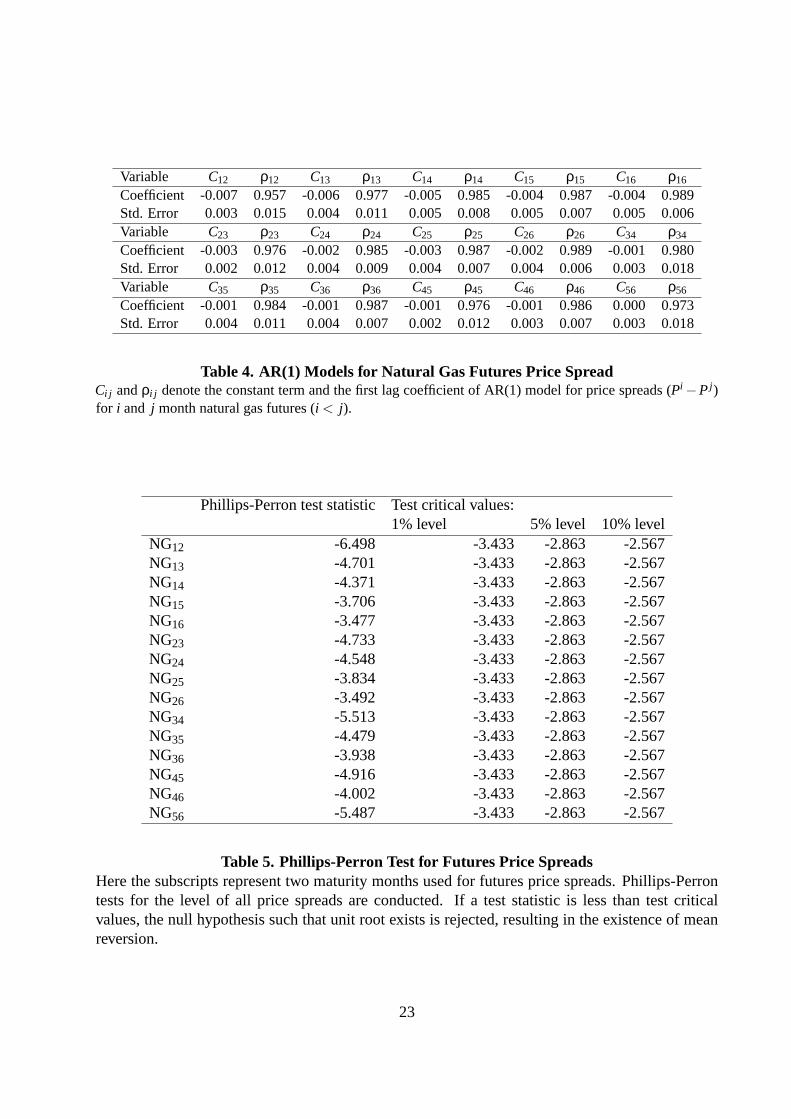
data are obtained from Bloomberg. Summary statistics for WTI, HO, and NG futures prices are

provided in Tables 1, 2, and 3, respectively. These tables indicate that WTI, HO, and NG have

common skewness characteristics. The skewness of WTI, HO, and NG futures prices is positive,

meaning that the distributions are skewed to the right.

[INSERT TABLE 1 ABOUT HERE]



5

3.2. The profit model for energy futures

Figure 1 shows the term structure of the NYMEX natural gas futures, which comprise six delivery

months (shown on the maturity axis) and whose daily observations cover from April 3, 2000 to

March 31, 2008 (shown on the time axis). As can be seen, the shape of the futures curve with six

delivery months fluctuates over the period. A closer look at Figure 1 illustrates that the futures

curve sometimes exhibits backwardation (e.g., April 2002) and at other times contango (e.g., April

2004).2 The existence of backwardation and contango at different moments gives rise to the exis-

tence of the flat term structure that switches from backwardation to contango, or vice versa. Thus,

energy futures prices that have different maturities converge on the flat term structure, even though

price deviates from the others due to the backwardation or contango. These attributes that we ob-

serve for the term structure of energy futures prices may be useful in obtaining the potential profit

in energy futures markets using the convergence of the price spread between the two correlated

assets as in spread trading. More importantly, the transition of price spreads from backwardation

or contango to the flat term structure can be considered as a mean reversion of the spread.

[INSERT FIGURE 1 ABOUT HERE]

In order to support this conjecture, we estimate the following autoregressive 1 lag (AR(1))

model for price spreads (Pi−P j ) for i and j month natural gas futures (i < j).

Pit −P j

t = Ci j +ρi j (Pit−1−P j

t−1)+ εt , (6)

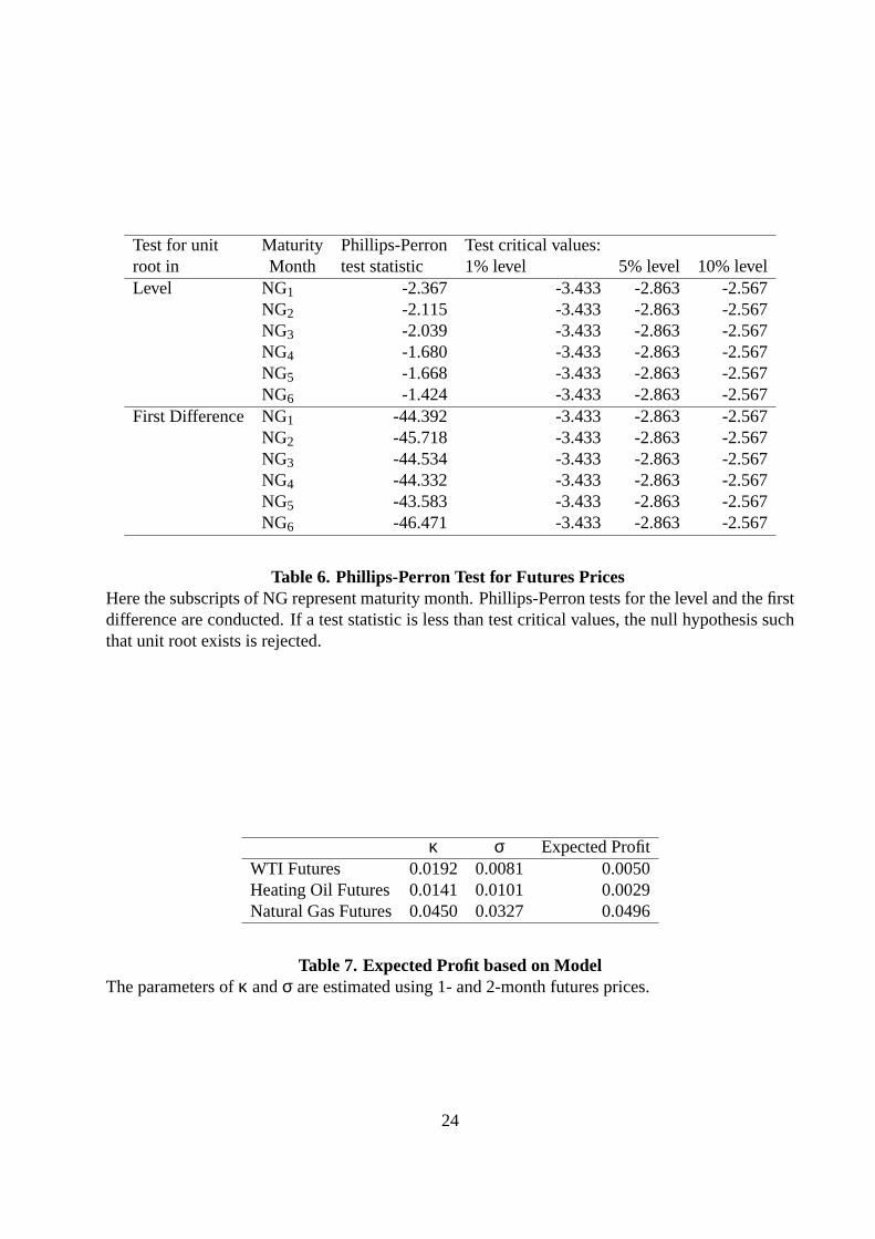
whereεt ∼ N(0,σ2i, j). The results are reported in Table 4. In addition, the Phillips-Perron tests

are conducted as unit root tests for stationarity not only for futures price spreads but also for each

delivery month futures prices, which are shown in Tables 5 and 6, respectively.




As can be seen from the table, AR(1) coefficients for all combinations of the price spreads are

statistically significant and greater than 0 and less than 1. In addition, the Phillips-Perron tests2When the futures curve increases in maturity, it is called “contango.” When it decreases in maturity, it is called

“backwardation.”

6

for the levels of price spreads all reject the existence of unit roots because the Phillips-Perron

test statistics are less than three test critical values. Moreover comparing Table 6 with Table 5,

the cointegration relationships between all two different maturity futures prices (Pi andPj ) exist

with long term relationship ofPi = Pj +Const because Tables 5 and 6 suggest that all futures

price spreads do not have any unit root and all futures prices have one unit root, respectively.

It may secure the convergence of the spread into a constant value. Given the characteristics of

the price spreads for energy futures that we observe, we conclude that a mean-reverting model

with long term mean can be applicable to energy futures price spreads. Hence as one of the

main modification to energy futures, we try to characterize the general profit model in Section 2

irrelevant to the type of stochastic price spread process by using a mean-reverting price spread

process for energy futures.

As a first-order approximation, we assume that the price spread of a spread trade, denoted by

St = Pit −P j

t , follows a mean-reverting process given by

dSt = κ(θ−St)dt+σdWt . (7)

Note thatκ = − lnρi j , θ = Ci j1−ρi j

, andσ = σi j

√−2lnρi j

1−ρ2i j

where we neglect the subscripts.κ andθ

represent mean reversion speed and long term mean, respectively. For simplicity, we assume that

κ, θ, andσ are constant. Equation (7) was used by Jurek and Yang (2007) as a general formulation

for an investor facing a mean-reverting arbitrage opportunity and by Dempster, Medova, and Tang

(2008) for valuing and hedging spread options on two commodity prices that are assumed to be

cointegrated in the long run. Since we define price spreads as the subtraction of longer maturity

product price from shorter maturity product price, positive and negative spreads (S’s) demonstrate

backwardation and contango, respectively. According to Table 4, the constant termsCi j tend to

be negative, resulting in the contango in respect to long run average price spreads. For example

regarding the futures price spreads between 1- and 2- month maturities,θ is calculated as -0.163

usingC12 =−0.007andρ12 = 0.957in Table 4, i.e., the negative price spread which subtracts 2-

month product from 1- month product, resulting in the contango. Hence if the futures prices often

demonstrate backwardation, the price spreads can theoretically produce profits from spread trades

in the long run. In addition, taking into account that long term mean parametersCi j are negative

but statistically insignificant exceptC12 in Table 4, strong contango may also produce profits from

the trades. Thus, the asymmetry in the profitability of the trading strategy depends on the statistical

significance of negative long term mean parameters (Ci j ) in the long run.

As another main modification of the general model to energy futures, computable first hitting

time density is employed. Linetsky (2004) provides an explicit analytical characterization for the

7

first hitting time (probability) density for a mean-reverting process that can be applied to modeling

interest rates, credit spreads, stochastic volatility, and convenience yields. By Proposition 2 in

Linetsky (2004), the first hitting time density of a mean-reverting process moving fromx to 0 is

approximately:

fτx→0(t)'∞

∑n=1

cnλne−λnt , (8)

whereλn andcn have the following large-n asymptotics:

λn = κ{

2kn− 12

},

cn' (−1)n+12√

kn

(2kn− 12)(π

√kn−2−

12 y)

e14(x2−y2) cos

(x√

2kn−πkn +π4

),

kn' n− 14

+y2

π2 +y√

2π

√n− 1

4+

y2

2π2 .

x andy are expressed by

x =√

2κσ

(x−θ) andy =√

2κσ

(−θ).

Thus, the profit model for the convergence case is modeled by

rp,c' x∞

∑n=1

cn(1−e−λnT)

. (9)

Next consider the case where there is a failure to converge during the trading period. Because

the price spreadSt follows a mean-reverting process, the corresponding probability density is given

by

g(y;x,T) =1√

2πσS(T)e− 1

2(y−µS(x,T))2

σS(T)2 , (10)

where

µS(x,T) = xe−κT +θ(1−e−κT) andσS(T) =√

σ2

2κ(1−e−2κT).

In addition, recall that the first hitting time density for a mean-reverting process is given by

equation (8). The expected profit from the failure to converge case is approximately modeled as

follows:

rp,nc'Z ∞

0(x−y)

{g(y;x,T)−

Z T

0

∞

∑n=1

cnλne−λntg(y;0,T− t)dt

}dy. (11)

8

Thus, the total profit model for spread trading is expressed by equation (5) whererp,c andrp,nc

are calculated from equations (9) and (11), respectively.

Since bothx and y embedded in the coefficients of equations (9) and (11) are expressed as

functions of the mean-reversion strength and volatility of the spread, denoted byκ andσ, respec-

tively in equation (7), the expected profit from a simple spread trading strategy is influenced by

the degree of mean reversion and volatility. More precisely, we have formulated the expected re-

turn from spread convergence and failure to converge cases using a simple mean-reverting spread

model characterized byκ andσ.

The model is not restricted to energy commodities but can be used for spread trading of other

commodities such as beans and beans oil. Hence, the model can be applicable to commodities

whose prices demonstrate strong mean reversion and high volatility. Because it is well known

that energy prices demonstrate strong mean reversion and high volatility (see Geman (2005)), the

model may fit energy commodities well.

3.3. Comparative statics of expected return

Since the profit model is based on a mean-reverting spread model, the expected returns are char-

acterized by the strength of mean reversion and volatility. We conducted comparative statics of

the expected return using the simple profit model we propose in equations (5), (9), and (11). As

a base case, we used the following values for the parameters of equation (7):κ = 0.027, θ =0, and σ = 0.013, which are estimated using the WTI one- and six- month spread. Moreover,

we assumed that the maturity is 120 days andx = 2σ. Based on the estimated parameters and the

assumptions made, we calculated the expected return for the simple profit model (rp) to be 0.0140.

Thus, the model predicts that the initial spread ofx = 2σ = 0.0260will produce a profit of 0.0140

from spread trading during a 120-day trading period.

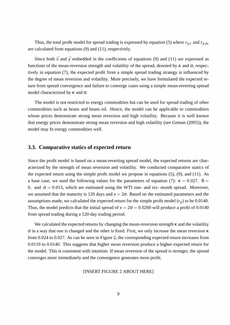
We calculated the expected returns by changing the mean-reversion strengthκ and the volatility

σ in a way that one is changed and the other is fixed. First, we only increase the mean reversionκfrom 0.024 to 0.027. As can be seen in Figure 2, the corresponding expected return increases from

0.0119 to 0.0140. This suggests that higher mean reversion produce a higher expected return for

the model. This is consistent with intuition: If mean reversion of the spread is stronger, the spread

converges more immediately and the convergence generates more profit.


9

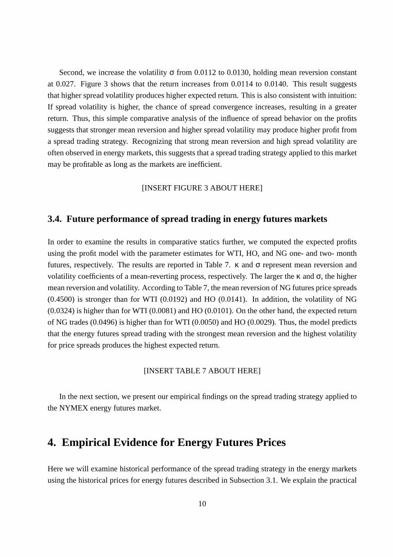
Second, we increase the volatilityσ from 0.0112 to 0.0130, holding mean reversion constant

at 0.027. Figure 3 shows that the return increases from 0.0114 to 0.0140. This result suggests

that higher spread volatility produces higher expected return. This is also consistent with intuition:

If spread volatility is higher, the chance of spread convergence increases, resulting in a greater

return. Thus, this simple comparative analysis of the influence of spread behavior on the profits

suggests that stronger mean reversion and higher spread volatility may produce higher profit from

a spread trading strategy. Recognizing that strong mean reversion and high spread volatility are

often observed in energy markets, this suggests that a spread trading strategy applied to this market

may be profitable as long as the markets are inefficient.


3.4. Future performance of spread trading in energy futures markets

In order to examine the results in comparative statics further, we computed the expected profits

using the profit model with the parameter estimates for WTI, HO, and NG one- and two- month

futures, respectively. The results are reported in Table 7.κ andσ represent mean reversion and

volatility coefficients of a mean-reverting process, respectively. The larger theκ andσ, the higher

mean reversion and volatility. According to Table 7, the mean reversion of NG futures price spreads

(0.4500) is stronger than for WTI (0.0192) and HO (0.0141). In addition, the volatility of NG

(0.0324) is higher than for WTI (0.0081) and HO (0.0101). On the other hand, the expected return

of NG trades (0.0496) is higher than for WTI (0.0050) and HO (0.0029). Thus, the model predicts

that the energy futures spread trading with the strongest mean reversion and the highest volatility

for price spreads produces the highest expected return.


In the next section, we present our empirical findings on the spread trading strategy applied to

the NYMEX energy futures market.

4. Empirical Evidence for Energy Futures Prices

Here we will examine historical performance of the spread trading strategy in the energy markets

using the historical prices for energy futures described in Subsection 3.1. We explain the practical

10

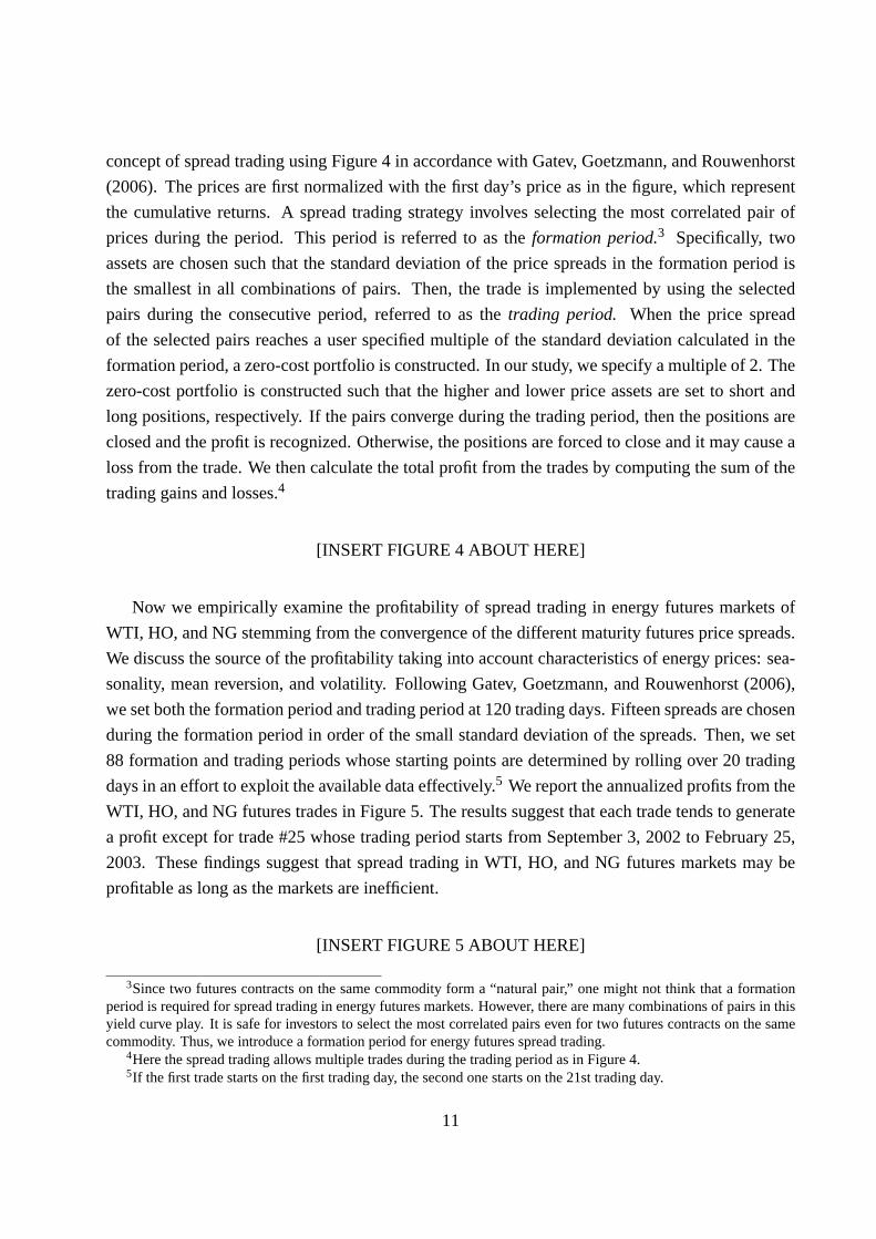
concept of spread trading using Figure 4 in accordance with Gatev, Goetzmann, and Rouwenhorst

(2006). The prices are first normalized with the first day’s price as in the figure, which represent

the cumulative returns. A spread trading strategy involves selecting the most correlated pair of

prices during the period. This period is referred to as theformation period.3 Specifically, two

assets are chosen such that the standard deviation of the price spreads in the formation period is

the smallest in all combinations of pairs. Then, the trade is implemented by using the selected

pairs during the consecutive period, referred to as thetrading period. When the price spread

of the selected pairs reaches a user specified multiple of the standard deviation calculated in the

formation period, a zero-cost portfolio is constructed. In our study, we specify a multiple of 2. The

zero-cost portfolio is constructed such that the higher and lower price assets are set to short and

long positions, respectively. If the pairs converge during the trading period, then the positions are

closed and the profit is recognized. Otherwise, the positions are forced to close and it may cause a

loss from the trade. We then calculate the total profit from the trades by computing the sum of the

trading gains and losses.4


Now we empirically examine the profitability of spread trading in energy futures markets of

WTI, HO, and NG stemming from the convergence of the different maturity futures price spreads.

We discuss the source of the profitability taking into account characteristics of energy prices: sea-

sonality, mean reversion, and volatility. Following Gatev, Goetzmann, and Rouwenhorst (2006),

we set both the formation period and trading period at 120 trading days. Fifteen spreads are chosen

during the formation period in order of the small standard deviation of the spreads. Then, we set

88 formation and trading periods whose starting points are determined by rolling over 20 trading

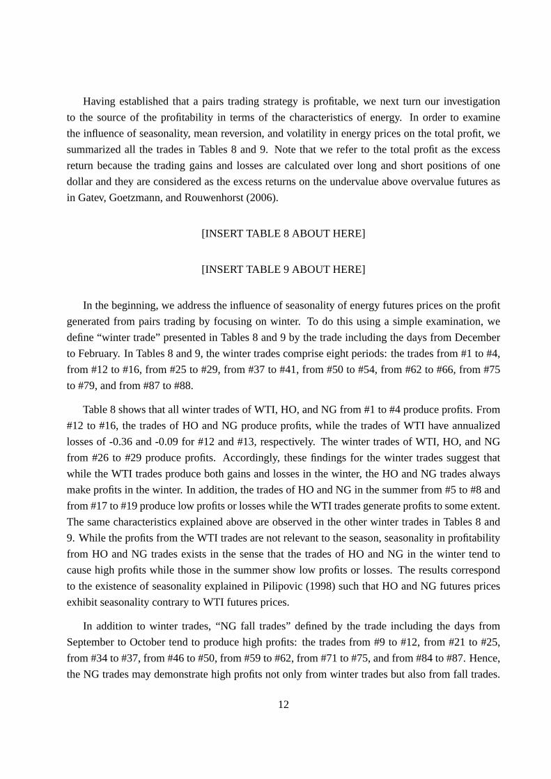
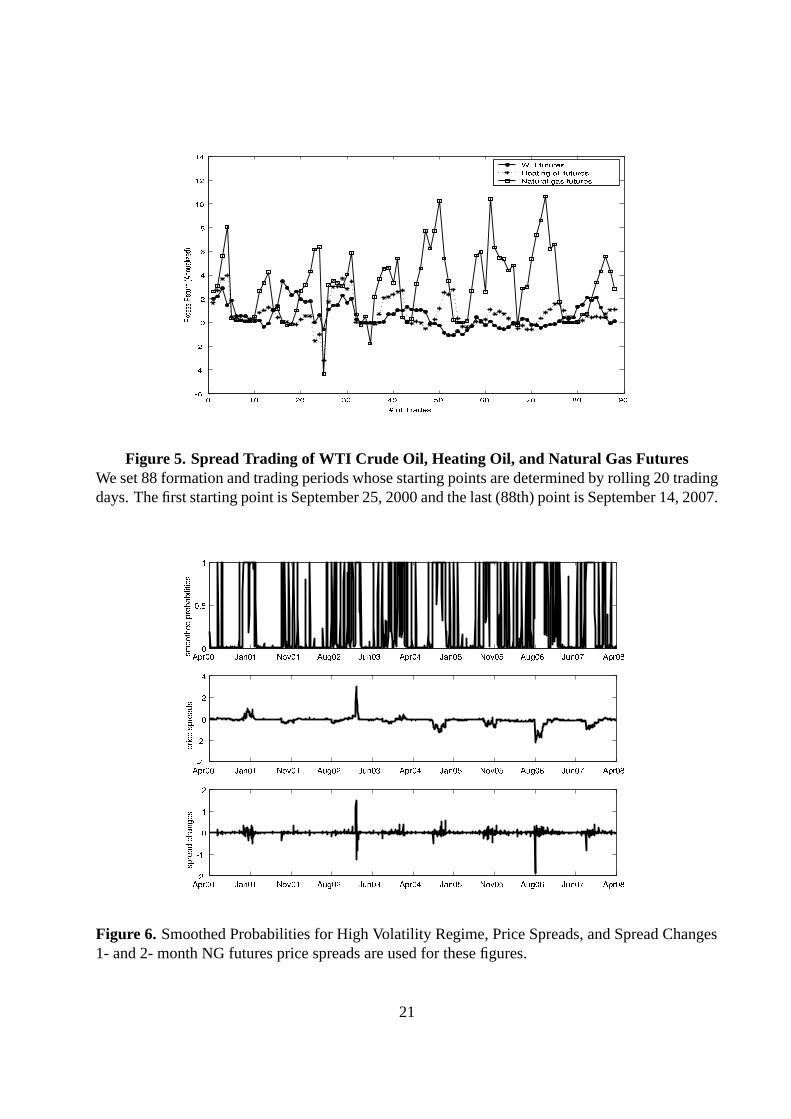
days in an effort to exploit the available data effectively.5 We report the annualized profits from the

WTI, HO, and NG futures trades in Figure 5. The results suggest that each trade tends to generate

a profit except for trade#25 whose trading period starts from September 3, 2002 to February 25,

2003. These findings suggest that spread trading in WTI, HO, and NG futures markets may be

profitable as long as the markets are inefficient.


3Since two futures contracts on the same commodity form a “natural pair,” one might not think that a formationperiod is required for spread trading in energy futures markets. However, there are many combinations of pairs in thisyield curve play. It is safe for investors to select the most correlated pairs even for two futures contracts on the samecommodity. Thus, we introduce a formation period for energy futures spread trading.

4Here the spread trading allows multiple trades during the trading period as in Figure 4.5If the first trade starts on the first trading day, the second one starts on the 21st trading day.

11

Having established that a pairs trading strategy is profitable, we next turn our investigation

to the source of the profitability in terms of the characteristics of energy. In order to examine

the influence of seasonality, mean reversion, and volatility in energy prices on the total profit, we

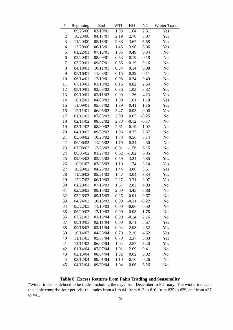
summarized all the trades in Tables 8 and 9. Note that we refer to the total profit as the excess

return because the trading gains and losses are calculated over long and short positions of one

dollar and they are considered as the excess returns on the undervalue above overvalue futures as

in Gatev, Goetzmann, and Rouwenhorst (2006).



In the beginning, we address the influence of seasonality of energy futures prices on the profit

generated from pairs trading by focusing on winter. To do this using a simple examination, we

define “winter trade” presented in Tables 8 and 9 by the trade including the days from December

to February. In Tables 8 and 9, the winter trades comprise eight periods: the trades from#1 to #4,

from #12to #16, from #25to #29, from #37to #41, from #50to #54, from #62to #66, from #75

to #79, and from#87to #88.

Table 8 shows that all winter trades of WTI, HO, and NG from#1 to #4 produce profits. From

#12 to #16, the trades of HO and NG produce profits, while the trades of WTI have annualized

losses of -0.36 and -0.09 for#12 and#13, respectively. The winter trades of WTI, HO, and NG

from #26 to #29 produce profits. Accordingly, these findings for the winter trades suggest that

while the WTI trades produce both gains and losses in the winter, the HO and NG trades always

make profits in the winter. In addition, the trades of HO and NG in the summer from#5 to #8 and

from #17to #19produce low profits or losses while the WTI trades generate profits to some extent.

The same characteristics explained above are observed in the other winter trades in Tables 8 and

9. While the profits from the WTI trades are not relevant to the season, seasonality in profitability

from HO and NG trades exists in the sense that the trades of HO and NG in the winter tend to

cause high profits while those in the summer show low profits or losses. The results correspond

to the existence of seasonality explained in Pilipovic (1998) such that HO and NG futures prices

exhibit seasonality contrary to WTI futures prices.

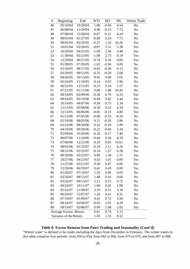
In addition to winter trades, “NG fall trades” defined by the trade including the days from

September to October tend to produce high profits: the trades from#9 to #12, from #21 to #25,

from #34to #37, from #46to #50, from #59to #62, from #71to #75, and from#84to #87. Hence,

the NG trades may demonstrate high profits not only from winter trades but also from fall trades.

12

It may imply that NG trade profits are generated not only during backwardation periods but also

during contango periods because high NG demand in winter often causes backwardation while

normal NG demand in fall demonstrates contango.

Since we are interested in the influence of seasonality on the total profit from energy futures

pairs trading, we compared the annualized average profits between WTI, HO, and NG. According

to the results reported in Table 9, the profits from six WTI, HO, and NG futures trades are 0.61,

0.74, and 3.15, respectively. We found that the NG trading generates the largest total profits (i.e.,

the highest excess return) of the three contracts investigated during the trading periods as in Table

9, while the HO and the WTI showed the second and the third highest excess return, respectively.

Since the profits from the WTI trades without seasonality are less than those from the HO and NG

trades with seasonality, this factor may determine the total profit.

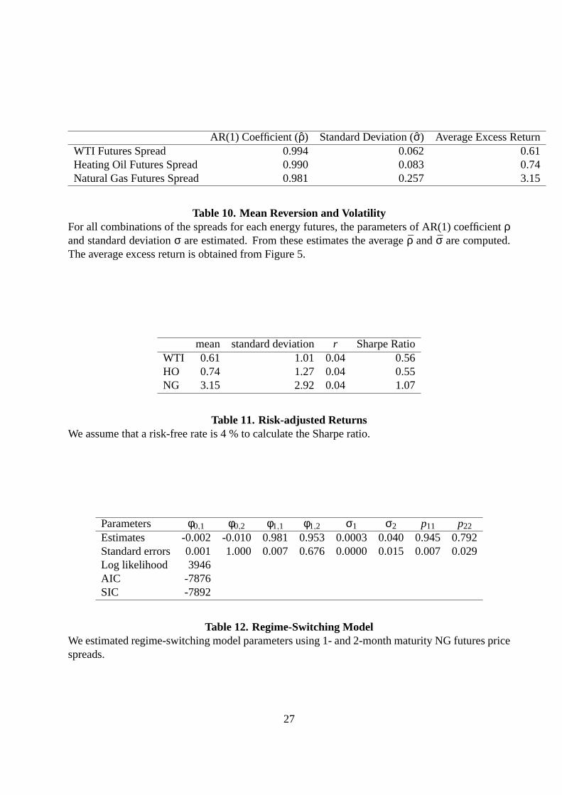
Next, we can shed light on the mean reversion and volatility of the spread as the source of the

total profits from spread trading. For all combinations of the spreads for each energy futures, we

estimate the parameters of AR(1) coefficientρ and standard deviationσ, which represent mean-

reversion strength and volatility, respectively, using equation (6). Then, we take the averageρandσ of the estimatedρ’s andσ’s, respectively, in order to capture the average trend of the mean

reversion and volatility of each energy futures market. The results are shown in Table 10. As

can be seen, the price spread of NG futures has the highest volatility of the three, because the

standard deviation is the largest (0.257) of the three. In addition while all three futures price

spreads demonstrate long term mean reversion, mean reversion of natural gas futures price spreads

is the strongest of the three. Considering that the NG trades generate the highest average return

(3.15) of the three, the highest total profit of spread trading applied to NG futures may come

from the highest volatility of the spread in addition to its long term mean reversion. The risk-

adjusted measure of performance is more persuasive in order to judge the performance. Thus,

we also calculated the risk-adjusted returns assuming a risk-free rate of 4% in Table 11 where

mean and standard deviation of returns are obtained from the results of Tables 8 and 9. Similar to

the average returns, the NG trades are more profitable than the others in terms of a risk-adjusted

measure of performance because the Sharpe ratio of the NG trades (1.07) is larger than those of

WTI (0.56) and HO (0.55). Thus, the highest risk-adjusted return of spread trading using NG

futures may also stem from the long term mean reversion and highest volatility of the spread.

Recalling that the comparative statics and future performance of spread trading in Subsections

3.3 and 3.4, respectively suggested that the long term mean reversion and high volatility of price

spreads may produce high performance of spread trading as long as the markets are inefficient, the

results in this section are consistent with the results from the comparative static analysis and future

performance of spread trading.

13



Finally in order to enhance the importance of price spread volatility for the trade profitability,

we apply a regime-switching model to NG futures price spreads where two regimes have different

volatility of σ1 andσ2, respectively and each process has mean reversion. Here we assume that

the state variablest evolves according to a first-order Markov chain, with transition probability

Pr(st = j | st−1 = i) = pi j . It indicates the probability of regime switching from statei at timet−1

to statej at timet. These probabilities are rewritten in the transition matrix:

P =

(p11 p21

p21 p22

)=

(p11 1− p22

1− p11 p22

). (12)

The regime switching model can be written as

St =

φ0,1 +φ1,1St−1 + ε1t

φ0,2 +φ1,2St−1 + ε2t

(13)

whereεit ∼ N(0,σ2

i ). We estimate the parameters of this model using 1- and 2-month NG futures

price spreads. The usual maximum likelihood method is applied by following e.g., Hamilton

(1994). The results are reported in Table 12. The parameters exceptφ0,2 andφ1,2 are statistically

significant. Taking into account thatσ2 is greater thanσ1, the state 1 and state 2 correspond to

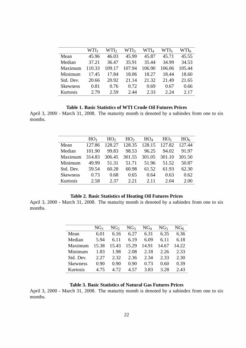
low and high volatility regimes, respectively. In addition, Figure 6 plots the smoothed probabilities

of high volatility regime using Kim (1993), corresponding price spreads, and spread changes. It

reports that high volatility regime tends to stand on high price spread and high spread change

periods, e.g., January 2001, October 2004, October 2005, and September 2006. Looking back

to Tables 8 and 9, it is observed that the NG trades during these high volatility regime periods

tend to produce high profits. For example, the trade#2 with high NG profit of 8.02 in Table

8 includes high volatility regime period of January 2001. Similarly high NG trade profits from

trades#50 (10.26),#61 (10.41), and#71 (8.59) and#73 (10.61) are obtained in high volatility

regime periods corresponding to October 2004, October 2005, and September 2006, respectively.

Hence, the results may also support our discussion such that high volatility produces high profit

from the trades. In addition, according to the middle picture of Figure 6, the profitable period

of January 2001 demonstrates backwardation because of positive price spreads while the other

profitable periods like October 2004 demonstrate contango. Hence both of backwardation and

contango seem to produce profits from NG trades. Furthermore, sinceφ1,2 is less than one but

14

statistically insignificant, the long term mean reversion may diminish during the high volatility

state period. It may imply that high volatility does not necessarily coincide with long term mean

reversion.



As is discussed, the results from the empirical analyses document that the long term mean

reversion and high volatility of price spreads may influence the total profit from spread trading of

energy futures, resulting in the support for the profit model we proposed in this paper.

5. Conclusions

In this paper, we provide a profit model for spread trading by focusing on the stochastic movement

of the price spread and its first hitting time probability density. The model is general in that it

does not specify the financial instrument. The advantage of the model is that the profit from

the trades can be easily calculated if the first hitting time probability density of the stochastic

process is given. Then the model was modified to fit energy futures by using a mean-reverting

process of the spreads, which reflects the characteristics of energy futures, with the computable first

hitting time density. The model predicted that future performance of pairs trading was enhanced

by strong mean reversion and high volatility of the price spreads. Our empirical analyses using

WTI crude oil, heating oil, and natural gas futures traded on the NYMEX show that pairs trading

in energy futures markets could produce a relatively stable profit in the past. Then, the sources

of the total profit were investigated from the characteristics of energy futures prices: seasonality,

mean reversion, and volatility. The total profits from heating oil and natural gas trading were

found to be positively affected by seasonality, contrary to the WTI crude oil, resulting in greater

total profits of heating oil and natural gas with seasonality than that of WTI crude oil without

seasonality. Seasonality may seem to characterize the total profit. More importantly, we examined

the influence of mean reversion and volatility of price spreads on the total profit. The results

suggest that the high volatility in addition to the long term mean reversion may cause high total

profits from pairs trading, especially in natural gas trades, which offers supportive evidence of the

model prediction.

The spread trading between energy commodity futures and their derivatives can be conducted

due to the influence of an increasing speculative tendency in the market e.g., for crude oil and

15

its derivatives. However this paper only dealt with the spread trading between different maturity

products for a single commodity due to the availability of the data. We leave this discussion for

our future research.

16

References

Dempster, M., E. Medova, and K. Tang, 2008, Long term spread option valuation and hedging,Journal of

Banking and Finance32, 2530–2540.

Emery, G. W., and Q. Liu, 2002, An analysis of the relationship between electricity and natural-gas futures

prices,Journal of Futures Markets22, 95–122.

Gatev, E.G., W. N. Goetzmann, and K. G. Rouwenhorst, 2006, Pairs trading: Performance of a relative-value

arbitrage rule,Review of Financial Studies19, 797–827.

Geman, H., 2005,Commodities and Commodity Derivatives. (John Wiley& Sons Ltd West Sussex).

Girma, P. B., and A. S. Paulson, 1998, Seasonality in petroleum futures spreads,Journal of Futures Markets

18, 581–598.

Girma, P. B., and A. S. Paulson, 1999, Risk arbitrage opportunities in petroleum futures spreads,Journal of

Futures Markets19, 931–955.

Hamilton, J. D., 1994,Time Series Analysis. (Princeton University Press Princeton).

Jurek, J., and H. Yang, 2007, Dynamic portfolio selection in arbitrage, Working paper, Harvard University.

Kim, C. J., 1993, Dynamic linear models with Markov-Switching,Journal of Econometrics1, 1–22.

Linetsky, V., 2004, Computing hitting time densities for CIR and OU diffusions: Applications to mean-

reverting models,Journal of Computational Finance7, 1–22.

Pilipovic, D., 1998,Energy Risk: Valuing and Managing Energy Derivatives. (McGraw-Hill New York).

17

Figures& Tables

��

��

��

��

��

�

�

�

� �

� �

� �

�

��

�� !"#$%&&' ()*

Figure 1. NYMEX Natural Gas Futures Curves

April 3, 2000 - March 31, 2008. NG futures product includes six delivery months – from one tosix months.

18

��

��

��

��

��

��

��

κ

��

Figure 2. Comparative Statics ofκ

By increasing the mean-reversion parameterκ from 0.024 to 0.027 holding volatility constant at0.0130, the corresponding expected returns for the simple profit model are shown.

��

��

��

��

��

��

��

σ

��

Figure 3. Comparative Statics ofσ

By increasing the volatility parameterσ from 0.0112 to 0.0130 holding mean reversion constantat 0.027, the corresponding expected returns for the simple profit model are shown.

19

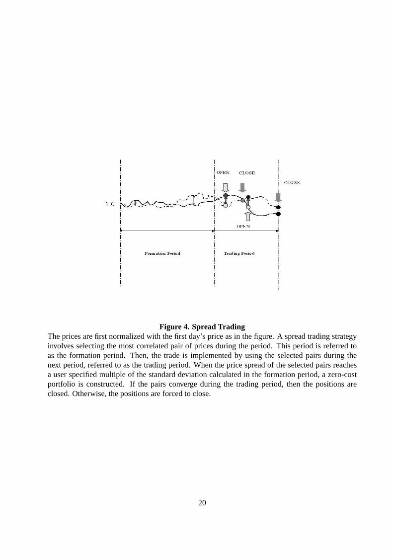
Figure 4. Spread TradingThe prices are first normalized with the first day’s price as in the figure. A spread trading strategyinvolves selecting the most correlated pair of prices during the period. This period is referred toas the formation period. Then, the trade is implemented by using the selected pairs during thenext period, referred to as the trading period. When the price spread of the selected pairs reachesa user specified multiple of the standard deviation calculated in the formation period, a zero-costportfolio is constructed. If the pairs converge during the trading period, then the positions areclosed. Otherwise, the positions are forced to close.

20

� ��

� �

� �

�

�

�

�

��

��

��

��

� �� !"#$"" %&' (�)*

+ �-,��/.�0/.��1 ��0/2 3�4��2 56�/.�0/.��7 ��0/.��564��8�/.�0/.��

Figure 5. Spread Trading of WTI Crude Oil, Heating Oil, and Natural Gas FuturesWe set 88 formation and trading periods whose starting points are determined by rolling 20 tradingdays. The first starting point is September 25, 2000 and the last (88th) point is September 14, 2007.

��

��

�

�� ! "# $%�& '&()( ("�

�� * �* �

�

��

$%( +"�$%"'# �

�� * �* �

��

�

�$%"'# +! ',-"�

Figure 6. Smoothed Probabilities for High Volatility Regime, Price Spreads, and Spread Changes1- and 2- month NG futures price spreads are used for these figures.

21

WTI1 WTI2 WTI3 WTI4 WTI5 WTI6

Mean 45.96 46.03 45.99 45.87 45.71 45.55Median 37.21 36.47 35.91 35.44 34.99 34.53Maximum 110.33 109.17 107.94 106.90 106.06 105.44Minimum 17.45 17.84 18.06 18.27 18.44 18.60Std. Dev. 20.66 20.92 21.14 21.32 21.49 21.65Skewness 0.81 0.76 0.72 0.69 0.67 0.66Kurtosis 2.79 2.59 2.44 2.33 2.24 2.17

Table 1. Basic Statistics of WTI Crude Oil Futures PricesApril 3, 2000 - March 31, 2008. The maturity month is denoted by a subindex from one to sixmonths.

HO1 HO2 HO3 HO4 HO5 HO6


Table 2. Basic Statistics of Heating Oil Futures PricesApril 3, 2000 - March 31, 2008. The maturity month is denoted by a subindex from one to sixmonths.

NG1 NG2 NG3 NG4 NG5 NG6


Table 3. Basic Statistics of Natural Gas Futures PricesApril 3, 2000 - March 31, 2008. The maturity month is denoted by a subindex from one to sixmonths.

22

Variable C12 ρ12 C13 ρ13 C14 ρ14 C15 ρ15 C16 ρ16

Coefficient -0.007 0.957 -0.006 0.977 -0.005 0.985 -0.004 0.987 -0.004 0.989Std. Error 0.003 0.015 0.004 0.011 0.005 0.008 0.005 0.007 0.005 0.006Variable C23 ρ23 C24 ρ24 C25 ρ25 C26 ρ26 C34 ρ34

Coefficient -0.003 0.976 -0.002 0.985 -0.003 0.987 -0.002 0.989 -0.001 0.980Std. Error 0.002 0.012 0.004 0.009 0.004 0.007 0.004 0.006 0.003 0.018Variable C35 ρ35 C36 ρ36 C45 ρ45 C46 ρ46 C56 ρ56

Coefficient -0.001 0.984 -0.001 0.987 -0.001 0.976 -0.001 0.986 0.000 0.973Std. Error 0.004 0.011 0.004 0.007 0.002 0.012 0.003 0.007 0.003 0.018

Table 4. AR(1) Models for Natural Gas Futures Price SpreadCi j andρi j denote the constant term and the first lag coefficient of AR(1) model for price spreads (Pi −P j )for i and j month natural gas futures (i < j).

Phillips-Perron test statistic Test critical values:1% level 5% level 10%level

NG12 -6.498 -3.433 -2.863 -2.567NG13 -4.701 -3.433 -2.863 -2.567NG14 -4.371 -3.433 -2.863 -2.567NG15 -3.706 -3.433 -2.863 -2.567NG16 -3.477 -3.433 -2.863 -2.567NG23 -4.733 -3.433 -2.863 -2.567NG24 -4.548 -3.433 -2.863 -2.567NG25 -3.834 -3.433 -2.863 -2.567NG26 -3.492 -3.433 -2.863 -2.567NG34 -5.513 -3.433 -2.863 -2.567NG35 -4.479 -3.433 -2.863 -2.567NG36 -3.938 -3.433 -2.863 -2.567NG45 -4.916 -3.433 -2.863 -2.567NG46 -4.002 -3.433 -2.863 -2.567NG56 -5.487 -3.433 -2.863 -2.567

Table 5. Phillips-Perron Test for Futures Price SpreadsHere the subscripts represent two maturity months used for futures price spreads. Phillips-Perrontests for the level of all price spreads are conducted. If a test statistic is less than test criticalvalues, the null hypothesis such that unit root exists is rejected, resulting in the existence of meanreversion.

23

Test for unit Maturity Phillips-Perron Test critical values:root in Month test statistic 1% level 5% level 10%levelLevel NG1 -2.367 -3.433 -2.863 -2.567

NG2 -2.115 -3.433 -2.863 -2.567NG3 -2.039 -3.433 -2.863 -2.567NG4 -1.680 -3.433 -2.863 -2.567NG5 -1.668 -3.433 -2.863 -2.567NG6 -1.424 -3.433 -2.863 -2.567

First Difference NG1 -44.392 -3.433 -2.863 -2.567NG2 -45.718 -3.433 -2.863 -2.567NG3 -44.534 -3.433 -2.863 -2.567NG4 -44.332 -3.433 -2.863 -2.567NG5 -43.583 -3.433 -2.863 -2.567NG6 -46.471 -3.433 -2.863 -2.567

Table 6. Phillips-Perron Test for Futures PricesHere the subscripts of NG represent maturity month. Phillips-Perron tests for the level and the firstdifference are conducted. If a test statistic is less than test critical values, the null hypothesis suchthat unit root exists is rejected.

κ σ Expected ProfitWTI Futures 0.0192 0.0081 0.0050Heating Oil Futures 0.0141 0.0101 0.0029Natural Gas Futures 0.0450 0.0327 0.0496

Table 7. Expected Profit based on ModelThe parameters ofκ andσ are estimated using 1- and 2-month futures prices.

24

# Beginning End WTI HO NG Winter Trade1 09/25/00 03/19/01 1.98 1.64 2.61 Yes2 10/23/00 04/17/01 2.19 2.70 3.07 Yes3 11/20/00 05/15/01 2.88 3.67 5.58 Yes4 12/20/00 06/13/01 1.45 3.98 8.06 Yes5 01/22/01 07/12/01 1.85 0.49 0.34 No6 02/20/01 08/09/01 0.53 0.19 0.18 No7 03/20/01 09/07/01 0.55 0.19 0.16 No8 04/18/01 10/11/01 0.54 0.14 0.08 No9 05/16/01 11/08/01 0.15 0.29 0.11 No

10 06/14/01 12/10/01 0.08 0.24 0.49 No11 07/13/01 01/10/02 0.16 0.82 2.64 No12 08/10/01 02/08/02 -0.36 1.03 3.32 Yes13 09/10/01 03/11/02 -0.09 1.26 4.23 Yes14 10/12/01 04/09/02 1.00 1.01 1.10 Yes15 11/09/01 05/07/02 1.39 0.41 1.16 Yes16 12/11/01 06/05/02 3.47 0.03 0.06 Yes17 01/11/02 07/03/02 2.90 0.03 -0.25 No18 02/11/02 08/02/02 2.30 -0.12 -0.17 No19 03/12/02 08/30/02 2.61 -0.19 1.02 No20 04/10/02 09/30/02 1.96 0.25 2.67 No21 05/08/02 10/28/02 1.73 0.56 3.14 No22 06/06/02 11/25/02 1.79 0.54 4.30 No23 07/08/02 12/26/02 -0.01 -1.56 6.15 No24 08/05/02 01/27/03 0.62 -1.02 6.35 No25 09/03/02 02/25/03 -0.59 -3.24 -4.35 Yes26 10/01/02 03/25/03 1.10 1.74 3.14 Yes27 10/29/02 04/23/03 1.44 3.00 3.51 Yes28 11/26/02 05/21/03 1.47 3.04 3.34 Yes29 12/27/02 06/19/03 2.27 3.71 3.07 Yes30 01/28/03 07/18/03 1.67 2.83 4.03 No31 02/26/03 08/15/03 2.00 3.45 5.88 No32 03/26/03 09/15/03 0.25 0.01 0.67 No33 04/24/03 10/13/03 0.00 -0.11 -0.22 No34 05/22/03 11/10/03 0.00 -0.06 0.50 No35 06/20/03 12/10/03 0.00 -0.08 -1.78 No36 07/21/03 01/13/04 0.00 -0.14 2.16 No37 08/18/03 02/11/04 0.00 0.71 3.67 Yes38 09/16/03 03/11/04 0.04 2.08 4.52 Yes39 10/14/03 04/08/04 0.70 2.16 4.62 Yes40 11/11/03 05/07/04 0.70 2.37 3.33 Yes41 12/11/03 06/07/04 1.04 2.57 5.40 Yes42 01/14/04 07/07/04 1.01 2.69 0.41 No43 02/13/04 08/04/04 1.32 0.02 0.02 No44 03/12/04 09/01/04 1.10 -0.10 0.26 No45 04/12/04 09/30/04 1.04 0.06 3.26 No

Table 8. Excess Returns from Pairs Trading and Seasonality“Winter trade” is defined to be trades including the days from December to February. The winter trades inthis table comprise four periods: the trades from#1 to #4, from #12to #16, from #25to #29, and from#37to #41.

25

# Beginning End WTI HO NG Winter Trade46 05/10/04 10/28/04 1.06 -0.04 4.54 No47 06/08/04 11/29/04 0.90 -0.53 7.72 No48 07/08/04 12/28/04 -0.07 -0.21 6.24 No49 08/05/04 01/27/05 -0.09 0.24 7.73 No50 09/02/04 02/25/05 -0.27 1.16 10.26 Yes51 10/01/04 03/28/05 -0.87 2.51 5.39 Yes52 10/29/04 04/25/05 -1.09 2.36 3.48 Yes53 11/30/04 05/23/05 -1.08 2.75 0.19 Yes54 12/29/04 06/21/05 -0.74 0.34 0.00 Yes55 01/28/05 07/20/05 -1.02 -0.36 0.00 No56 02/28/05 08/17/05 -0.65 -0.39 0.13 No57 03/29/05 09/15/05 -0.33 -0.28 2.68 No58 04/26/05 10/13/05 0.45 0.08 5.65 No59 05/24/05 11/10/05 0.14 0.02 5.96 No60 06/22/05 12/12/05 -0.23 0.24 2.57 No61 07/21/05 01/11/06 0.08 1.08 10.41 No62 08/18/05 02/09/06 -0.26 0.70 6.33 Yes63 09/16/05 03/10/06 -0.49 0.92 5.44 Yes64 10/14/05 04/07/06 -0.58 0.73 5.34 Yes65 11/11/05 05/08/06 -0.39 0.33 4.38 Yes66 12/13/05 06/06/06 -0.05 -0.15 4.80 Yes67 01/12/06 07/05/06 -0.06 -0.53 -0.26 No68 02/10/06 08/02/06 0.31 -0.26 2.86 No69 03/13/06 08/30/06 0.22 -0.59 2.99 No70 04/10/06 09/28/06 -0.22 -0.60 5.34 No71 05/09/06 10/26/06 -0.26 -0.17 7.40 No72 06/07/06 11/24/06 -0.46 0.36 8.59 No73 07/06/06 12/22/06 -0.29 0.83 10.61 No74 08/03/06 01/25/07 -0.19 1.11 6.20 No75 08/31/06 02/23/07 -0.14 1.57 6.58 Yes76 09/29/06 03/23/07 0.09 1.58 1.75 Yes77 10/27/06 04/23/07 0.43 1.01 0.00 Yes78 11/27/06 05/21/07 0.30 0.47 0.00 Yes79 12/26/06 06/19/07 0.42 0.45 0.00 Yes80 01/26/07 07/18/07 1.33 0.00 0.05 No81 02/26/07 08/15/07 1.48 0.16 0.66 No82 03/26/07 09/13/07 2.11 0.55 0.72 No83 04/24/07 10/11/07 1.84 0.42 1.99 No84 05/22/07 11/09/07 2.10 0.51 3.36 No85 06/20/07 12/07/07 1.26 0.41 4.31 No86 07/19/07 01/09/07 0.41 0.72 5.56 No87 08/16/07 02/06/07 -0.05 1.05 4.29 Yes88 09/14/07 03/06/07 0.09 1.08 2.82 YesAverage Excess Return 0.61 0.74 3.15Variance of the Return 1.03 1.53 8.52

Table 9. Excess Returns from Pairs Trading and Seasonality (Cont’d)“Winter trade” is defined to be trades including the days from December to February. The winter trades inthis table comprise four periods: from#50to #54, from #62to #66, from #75to #79, and from#87to #88.

26

AR(1) Coefficient (ρ) Standard Deviation (σ) Average Excess ReturnWTI Futures Spread 0.994 0.062 0.61Heating Oil Futures Spread 0.990 0.083 0.74Natural Gas Futures Spread 0.981 0.257 3.15

Table 10. Mean Reversion and VolatilityFor all combinations of the spreads for each energy futures, the parameters of AR(1) coefficientρand standard deviationσ are estimated. From these estimates the averageρ andσ are computed.The average excess return is obtained from Figure 5.

mean standard deviation r Sharpe RatioWTI 0.61 1.01 0.04 0.56HO 0.74 1.27 0.04 0.55NG 3.15 2.92 0.04 1.07

Table 11. Risk-adjusted ReturnsWe assume that a risk-free rate is 4% to calculate the Sharpe ratio.

Parameters φ0,1 φ0,2 φ1,1 φ1,2 σ1 σ2 p11 p22

Estimates -0.002 -0.010 0.981 0.953 0.0003 0.040 0.945 0.792Standard errors 0.001 1.000 0.007 0.676 0.0000 0.015 0.007 0.029Log likelihood 3946AIC -7876SIC -7892

Table 12. Regime-Switching ModelWe estimated regime-switching model parameters using 1- and 2-month maturity NG futures pricespreads.

27

No. 27

No. 26

No. 25

No. 24

No. 23

No. 22

No. 21

No. 20

No. 19

No.18

No. 17

Takashi Kanamura, Svetlozar T. Rachev, Frank J. Fabozzi: A profit model

for spread trading with an application to energy futures, May 2011

Michele Leonardo Bianchi, Svetlozar T. Rachev, Young Shin Kim, Frank J.

Fabozzi: Tempered infinitely divisible distributions and processes, May

2011

Sebastian Kube, Michel André Maréchal and Clemens Puppe: The curren-

cy of reciprocity - gift-exchange in the workplace, April 2011

Clemens Puppe and Attila Tasnádi: Axiomatic districting, April 2011

Dinko Dimitrov and Clemens Puppe: Non-bossy social classification, April

2011

Kim Kaivanto and Eike B. Kroll: Negative recency, randomization device

choice, and reduction of compound lotteries, April 2011

Antje Schimke and Thomas Brenner: Long-run factors of firm growth - a

study of German firms, April 2011

Aaron B. Scholz: Spatial network configurations of cargo airlines, April

2011

Arne Beck: Public bus transport in Germany - a proposal to improve the

current awarding system, April 2011

Nina Menz and Ingrid Ott: On the role of general purpose technologies

within the Marshall-Jacobs controversy: the case of nanotechnologies,

April 2011

Berno Buechel: A note on Condorcet consistency and the median voter,

April 2011

recent issues

Working Paper Series in Economics

The responsibility for the contents of the working papers rests with the author, not the Institute. Since working papers

are of a preliminary nature, it may be useful to contact the author of a particular working paper about results or ca-

veats before referring to, or quoting, a paper. Any comments on working papers should be sent directly to the author.

a profit model for spread trading with an application to...

Documents