a probabilistic model for software defect prediction - researchgate

For submission to IEEE Transactions in Software Engineering

A Probabilistic Model for Software Defect Prediction

Norman Fenton, Paul Krause and Martin Neil

• = Please address all correspondence to: Paul Krause

Index Terms:

Software Reliability; Graphical Probabilistic Models; Defect Estimation; Software Process Improvement.

Contact details for Professor Norman Fenton: Queen Mary, University of London and Agena Ltd. Mile End Road London E1 4NS Tel: +44 (0) 20 7882 7860 Mobile: 07932 030084 Fax: +44 (0) 870 131 8460 e-mail: [email protected]

Contact details for Dr. Paul Krause: Philips Research Laboratories Crossoak Lane Redhill Surrey RH1 5HA Tel: +44 (0) 1293 815298 Fax: +44 (0) 1293 815500 e-mail: [email protected]

Contact details for Dr. Martin Neil: Queen Mary, University of London and Agena Ltd. Mile End Road London E1 4NS Tel: +44 (0) 20 7882 5221 Mobile: 0411 956 330 Fax: +44 (0) 870 131 8460 e-mail: [email protected]


2 of 2

Abstract

Although a number of approaches have been taken to quality prediction for software, none have achieved

widespread applicability. Our aim here is to produce a single model to combine the diverse forms of, often

causal, evidence available in software development in a more natural and efficient way than done

previously. We use graphical probability models (also known as Bayesian Belief Networks) as the

appropriate formalism for representing this evidence. We can use the subjective judgements of experienced

project managers to build the probability model and use this model to produce forecasts about the software

quality throughout the development life cycle. Moreover, the causal or influence structure of the model

more naturally mirrors the real world sequence of events and relations than can be achieved with other

formalisms. The paper focuses on the particular model that has been developed for Philips Software Centre

(PSC), using expert knowledge from Philips Research Labs. The model is used especially to predict defect

rates at various testing and operational phases. To make the model usable by software quality managers we

have developed a tool (AID) and have used it to validate the model on 28 diverse projects at PSC. In each

of these projects, extensive historical records were available. The results of the validation are encouraging.

In most cases the model provides accurate predictions of defect rates even on projects whose size was

outside the original scope of the model.

1 Introduction

Important decisions need to be made during the course of developing software products. Perhaps the most

important of these is the decision when to release the software product. The consequences of making an ill-

judged decision can be potentially critical for the reputation of a product or its supplier. Yet, such decisions

are often made informally, rather than on the basis of more objective and accountable criteria.

Software project and quality managers must juggle a combination of uncertain factors, such as tools,

personnel, development methods and testing strategies to achieve the delivery of a quality product to

budget and on time. Each of these uncertain factors influences the introduction, detection and correction of

defects at all stages in the development life cycle from initial requirements to product delivery.

In order to achieve software quality during development special emphasis needs to be applied to the

following three activities in particular:


3 of 3

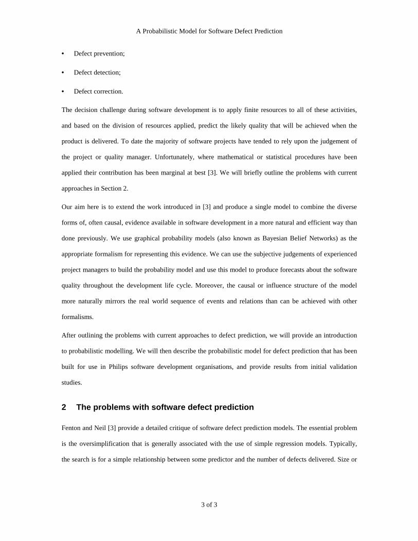
• = Defect prevention;

• = Defect detection;

• = Defect correction.

The decision challenge during software development is to apply finite resources to all of these activities,

and based on the division of resources applied, predict the likely quality that will be achieved when the

product is delivered. To date the majority of software projects have tended to rely upon the judgement of

the project or quality manager. Unfortunately, where mathematical or statistical procedures have been

applied their contribution has been marginal at best [3]. We will briefly outline the problems with current

approaches in Section 2.

Our aim here is to extend the work introduced in [3] and produce a single model to combine the diverse

forms of, often causal, evidence available in software development in a more natural and efficient way than

done previously. We use graphical probability models (also known as Bayesian Belief Networks) as the

appropriate formalism for representing this evidence. We can use the subjective judgements of experienced

project managers to build the probability model and use this model to produce forecasts about the software

quality throughout the development life cycle. Moreover, the causal or influence structure of the model

more naturally mirrors the real world sequence of events and relations than can be achieved with other

formalisms.

After outlining the problems with current approaches to defect prediction, we will provide an introduction

to probabilistic modelling. We will then describe the probabilistic model for defect prediction that has been

built for use in Philips software development organisations, and provide results from initial validation

studies.

2 The problems with software defect prediction

Fenton and Neil [3] provide a detailed critique of software defect prediction models. The essential problem

is the oversimplification that is generally associated with the use of simple regression models. Typically,

the search is for a simple relationship between some predictor and the number of defects delivered. Size or


4 of 4

complexity measures are often used as such predictors. The result is a naïve model that could be

represented by the graph of Figure 2.1(a). Figure 2.1 about here.

The difficulty is that whilst such a model can be used to explain a data set obtained in a specific context,

none has so far been subject to the form of controlled statistical experimentation needed to establish a

causal relationship. Indeed, the analysis of Fenton and Neil suggests that these models fail to include all the

causal or explanatory variables needed in order to make the models generalisable. Further strong empirical

support for these arguments is demonstrated in [4].

As an example, in investigating the relationship between two variables such as S and D in Figure 2.1, one

would at least wish to differentiate between a direct causal relationship and the influence of some common

cause as a “hidden variable”. For example, we might hypothesise “Problem Complexity” (PC) as a

common cause for our two variables S and D, Figure 2.1(b).

The model of Figure 2.1(a) can simulate the model of Figure 2.1(b) under certain circumstances. However,

the latter has greater explanatory power, and can lead to quite a different interpretation of a set of data. One

could take “Smoking” and “Higher Grades” at high school as an analogy. Just looking at the covariance

between the two variables, we might see a correlation between smoking and achieving higher grades.

However, if "Age" is then included in the model, we could have a very different interpretation of the same

data. As a student's age increases, so does the likelihood of their smoking. As they mature, their grades also

typically improve. The covariance is explained. However, for any fixed age group, smokers may achieve

lower grades than non-smokers.

We believe that the relationships between product and process attributes and numbers of defects are too

complex to admit straightforward curve fitting models. In predicting defects discovered in a particular

project, we would certainly want to add additional variables to the model of Figure 2.1(a). For example, the

number of defects discovered will depend on the effectiveness with which the software is tested. It may

also depend on the level of detail of the specifications from which the test cases are derived, the care with

which requirements have been managed during product development, and so on. We believe that graphical

probabilistic models are the best candidates for situations with such a rich causal structure.


5 of 5

3 Introduction to probabilistic models

3.1 Conditional probability

Probabilities conform to three basic axioms:

• = p(A), the probability of an event (outcome/consequence…), A, is a number between 0 and 1;

• = p(A)=0 means A is impossible, p(A)=1 means A is certain;

• = p(A or B) = p(A) + p(B) provided A and B are disjoint.

However, merely to refer to the probability p(H) of an event or hypothesis is an oversimplification. In

general, probabilities are context sensitive. For example, the probability of suffering from certain forms of

cancer is higher in Europe than it is in Asia. Strictly, the probability of any event or hypothesis is

conditional on the available evidence or current context. This can be made explicit by the notation p(H | E),

which is read as “the probability of H given the evidence E”. In the coin example, H would be a “heads”

event and E an explicit reference to the evidence that the coin is a fair one. If there was evidence E' that the

coin was double sided heads, then we would have p(H | E') = 1.0.

As soon as we start thinking in terms of conditional probabilities, we begin to need to think about the

structure of problems as well as the assignment of numbers. To say that the probability of an hypothesis is

conditional on one or more items is to identify the information relevant to the problem at hand. To say that

the identification of an item of evidence influences the probability of an hypothesis being valid is to place a

directionality on the links between evidences and hypotheses.

Often a direction corresponding to causal influence can be the most meaningful. For example, in medical

diagnosis one can in a certain sense say that measles “causes” red spots (there might be other causes). So,

as well as assigning a value to the conditional p(‘red spots’ | measles), one might also wish to provide an

explicit graphical representation of the problem. In this case we would simply draw an arrow from

“measles” to “red-spots”.

Note that to say that p(‘red spots’ | measles) = p means that we can assign probability p to ‘red spots’ if

measles is observed and only measles is observed. If any further evidence E is observed, then we will be

required to determine p(‘red spots’ | measles, E). The comma inside the parentheses denotes conjunction.


6 of 6

Building up a graphical representation can be a great aid in framing a problem. A significant recent

advance in probability theory has been the demonstration of a formal equivalence between the structure of

a graphical model and the dependencies that are expressed by a numerical probability distribution. In

numerical terms, we say that event A is independent of event B if observation of B makes no difference to

the probability that A will occur: p(A | B) = p(A). In graphical terms we indicate that A is independent of B

by the absence of any direct arrow between the nodes representing A and B in a graphical model.

So far, we have concentrated on the static aspects of assessing probabilities and indicating influences.

However, probability is a dynamic theory; it provides a mechanism for coherently revising the probabilities

of events as evidence becomes available. Conditional probability and Bayes’ Theorem play a central role in

this. We will use a simple example to illustrate Bayesian updating, and then introduce Bayes’ Theorem in

the next section.

Suppose we are interested in the number of defects that are detected and fixed in a certain testing phase. If

the software under test had been developed to high standards, perhaps undergoing formal reviews before

release to the test phase, then the high quality of the software would in a sense “cause” a low number of

defects to be detected in the test phase. However, if the testing were ineffective and superficial, then this

would provide an alternative cause for a low number of defects being detected during the test phase. (This

was precisely the common empirical scenario identified in [4]).

This situation can be represented by the simple graphical model of figure 3.1. Here the nodes in the graph

could represent simple binary variables with states “low” and “high”, perhaps. However, in general a node

may have many alternative states or even represent a continuous variable. We will stay with the binary

states for ease of discussion. Figure 3.1 about here.

It can be helpful to think of figure 3.1 as a fragment of a much larger model. In particular, the node SQ

(“Software Quality”) could be a synthesis of, for example: review effectiveness; developer’s skill level;

quality of input specifications; and, resource availability. With appropriate probability assignments to this

model, a variety of reasoning styles can be modelled. A straightforward reasoning from cause to effect is

possible. If TE (test effectiveness) is “low”, then the model will predict that DD (defects discovered and


7 of 7

fixed) will also be low. If earlier evidence indicates SQ (software quality) is “high”, then again DD will be

“low”.

However, an important feature is that although conditional probabilities may have been assessed in terms of

effect given cause, Bayes’ rule enables inference to be performed in the “reverse” direction – to provide the

probabilities of potential causes given the observation of some effect. In this case, if DD is observed to be

“low” the model will tell us that low test effectiveness or high software quality are possible explanations

(perhaps with an indication as to which one is the most likely explanation). The concept of “explaining

away” will also be modelled. For example, if we also have independent evidence that the software quality

was indeed high, then this will provide sufficient explanation of the observed value for DD and the

probability that test effectiveness was low will be reduced.

This situation can be more formally summarised as follows. If we have no knowledge of the state DD then

nodes TE and SQ are marginally independent – knowledge of the state of one will not influence the

probability of the other being in any of its possible states. However, nodes TE and SQ are conditionally

dependent given DD – once the state of DD is known there is an influence (via DD) between TE and SQ as

described above.

We will see in the next section that models of complex situations can be built up by composing together

relatively simple local sub-models of the above kind (See also [11]). This is enormously valuable. Without

being able to structure a problem in this way it can be virtually impossible to assess probability

distributions over large numbers of variables. In addition, the computational problem of updating such a

probability distribution given new evidence would be intractable.

3.2 Bayes’ theorem and graphical models

As indicated in the previous section, probability is a dynamic theory; it provides a mechanism for

coherently revising the probabilities of events as evidence becomes available. Bayes’ theorem is a

fundamental component of the dynamic aspects.

As mentioned earlier, we write p(A | B) to represent the probability of some event (an hypothesis)

conditional on the occurrence of some event B (evidence). If we are counting sample events from some

universe Ω, then we are interested in the fraction of events B for which A is also true. In effect we are


8 of 8

focusing attention from the universe Ω to a restricted subset in which B holds. From this it should be clear

that (with the comma denoting conjunction of events):

)(),(

)|(Bp

BApBAp =

This is the simplest form of Bayes’ rule. However, it is more usually rewritten in a form that tells us how to

obtain a posterior probability in a hypothesis A after observation of some evidence B, given the prior

probability in A and the likelihood of observing B were A to be the case:

)()()|(

)|(Bp

ApABpBAp =

This theorem is of immense practical importance. It means that we can reason both in a forward direction

from causes to effects, and in a reverse direction (via Bayes’ rule) from effects to possible causes. That is,

both deductive and abductive modes of reasoning are possible.

However, two significant problems need to be addressed. Although in principle we can use generalisations

of Bayes’ rule to update probability distributions over sets of variables, in practice:

1) Eliciting probability distributions over sets of variables is a major problem. For example, suppose we

had a problem describable by seven variables each with two possible states. Then we will need to elicit

(27-1) distinct values in order to be able to define the probability distribution completely. As can be

seen, the problem of knowledge elicitation is intractable in the general case.

2) The computations required to update a probability distribution over a set of variables are similarly

intractable in the general case.

Up until the late 1980’s, these two problems were major obstacles to the rigorous use of probabilistic

methods in computer based reasoning models. However, work initiated by Lauritzen and Spiegelhalter [8]

and Pearl [12] provided a resolution to these problems for a wide class of problems. This work related the

independence conditions described in graphical models to factorisations of the joint distributions over sets

of variables. We have already seen some simple examples of such models in the previous section. In

probabilistic terms, two variables X and Y are independent if p(X,Y) = p(X)p(Y) – the probability

distribution over the two variables factorises into two independent distributions. This is expressed in a


9 of 9

graphic by the absence of a direct arrow expressing influence between the two variables. Figure 3.2 about

here.

We could introduce a third variable Z, say, and state that “X is conditionally independent of Y given Z”.

This is expressed graphically in Figure 3.2. An expression of this in terms of probability distributions is:

p(X,Y | Z) = p(X | Z)p(Y | Z)

A significant feature of the graphical structure of Figure 3.2 is that we can now decompose the joint

probability distribution for the variables X, Y and Z into the product of terms involving at most two

variables: p(X,Y,Z) = p(X | Z)p(Y | Z)p(Z)

In a similar way, we can decompose the joint probability distribution for the variables associated with the

nodes DD, TE and SQ of Figure 3.1 as: p(DD, TE, SQ) = p(DD | TE,SQ)p(TE)p(SQ)

This gives us a series of example cases where a graph has admitted a simple factorisation of the

corresponding joint probability distribution. If the graph is directed (the arrows all have an associated

direction) and there are no cycles in the graph, then this property is a general one. Such graphs are called

Directed Acyclic Graphs (DAGs). Using a slightly imprecise notation for simplicity, we have [8]:

Proposition

Let U = X1, X2, …, Xn have an associated DAG G. Then the joint probability distribution p(U) admits a

direct factorisation:

))(|()(1

∏=

=n

i

ii XpaXpUp

Here pa(Xi) denotes a value assignment to the parents of Xi. (If an arrow in a graph is directed from A to B,

then A is a parent node and B a child node).

The net result is that the probability distribution for a large set of variables may be represented by a product

of the conditional probability relationships between small clusters of semantically related propositions.

Now, instead of needing to elicit a joint probability distribution over a set of complex events, the problem

is broken down into the assessment of these conditional probabilities as parameters of the graphical

representation.


10 of 10

The lessons from this section can be summarised quite succinctly. First, graphs may be used to represent

qualitative influences in a domain. Secondly, the conditional independence statements implied by the graph

can be used to factorise the associated probability distribution. This factorisation can then be exploited to

(a) ease the problem eliciting the global probability distribution, and (b) allow the development of

computationally efficient algorithms for updating probabilities on the receipt of evidence. We will now

describe how these techniques have been exploited to produce a probabilistic model for software defect

prediction.

4 The Probabilistic Model for Defect Prediction

Probabilistic models are a good candidate solution for an effective model of software defect prediction for

the following reasons:

1. They can easily model causal influences between variables in a specified domain;

2. The Bayesian approach enables statistical inference to be augmented by expert judgement in those

areas of a problem domain where empirical data is sparse;

3. As a result of the above, it is possible to include variables in a software reliability model that

correspond to process as well as product attributes;

4. Assigning probabilities to reliability predictions means that sound decision making approaches using

classical decision theory can be supported.

Our goal was to build a module level defect prediction model which could then be evaluated against real

project data. Although it was not possible to use members of Philips' development organisations directly to

perform extensive knowledge elicitation, PRL were able to act as a surrogate because of their experience

from working directly with Philips business units. This had the added advantage that the probabilistic

network could be built relatively quickly. However, the fact that the probability tables were in effect built

from “rough” information sources and strengths of relations necessarily limits the precision of the model.

The remainder of this section will provide an overview of the model to indicate the product and process

factors that are taken into account when a quality assessment is performed using it.


11 of 11

4.1 Overall structure of the probabilistic network

The probabilistic network is executed using the generic probabilistic inference engine Hugin (see

http://www.hugin.com for further details). However, the size and complexity of the network were such that

it was not realistic to attempt to build the network directly using the Hugin tool. Instead, Agena Ltd used

two methods and tools that are built on top of the Hugin propagation engine:

• = The SERENE method and tool [13], which enables: large networks to be built up from smaller ones in

a modular fashion; and, large probability tables to be built using pre-defined mathematical functions

and probability distributions.

• = The IMPRESS method and tool [6], which extends the SERENE tool by enabling users to generate

complex probability distributions simply by drawing distribution shapes in a visual editor.

The resulting network takes account of a range of product and process factors from throughout the lifecycle

of a software module. Because of the size of the model, it is impractical to display it in a single figure.

Instead, we provide a first schematic view in terms of sub-nets (Figure 4.1). This modular structure is the

actual decomposition that was used to build the network using the SERENE tool.

The main sub-nets in the high-level structure correspond to key software life-cycle phases in the

development of a software module. Thus there are sub-nets representing the specification phase, the

specification review phase, the design and coding phase and the various testing phases. Two further sub-

nets cover the influence of requirements management on defect levels, and operational usage on defect

discovery. The final defect density sub-net simply computes the industry standard defect density metric in

terms of residual defects delivered divided by module size. Figure 4.1 about here.

This structure was developed using the software development processes from a number of Philips

development units as models. A common software development process is not currently in place within

Philips. Hence the resulting structure is necessarily an abstraction. Again, this will limit the precision of the

resulting predictions. Work is in progress to develop tools to enable the structure to be customised to

specific development processes.

The arc labels in Figure 4.1 represent ‘joined’ nodes in the underlying sub-nets. This means that

information about the variables representing these joined nodes is passed directly between sub-nets. For


12 of 12

example, the specfication quality and the defect density sub-nets are joined by an arc labelled ‘Module

size’. This node is common to both sub-nets. As a result, information about the module size arising from

the specification quality sub-net is passed directly to the defect density sub-net. We refer to ‘Module size’

as an ‘output node’ for the specification quality sub-net, and an ‘input node’ for the defect density sub-net.

The figures in the following sub-sections show details of a number of sub-nets. In these figures, the dark

shaded nodes with dotted edges are output nodes, and the dark shaded ones with solid edges are input

nodes.

4.2 The specification quality sub-net

Figure 4.2 illustrates the Specification quality sub-net. It can be explained in the following way:

specification quality is influenced by three major factors: Figure 4.2 about here.

• = the intrinsic complexity of the module (this is the complexity of the requirements for the module,

which ranges from “very simple” to “very complex”);

• = the internal resources used, which is in turn defined in terms of the staff quality (ranging from “poor”

to “outstanding”), the document quality (meaning the quality of the initial requirements specification

document, ranging from “very poor” to “very good”), and the schedule constraints which ranges from

“very tight” to “very flexible”;

• = the stability of the requirements, which in turn is defined in terms of the novelty of the module

requirements (ranging from “very high” to “very low”) and the stakeholder involvement (ranging from

“very low” to “very high”). The stability node is defined in such a way that low novelty makes

stakeholder involvement irrelevant (Philips would have already built a similar relevant module), but

otherwise stakeholder involvement is crucial.

The specification quality directly influences the number of specification defects (which is an output node

with an ordinal scale that ranges from 0 to 10 – here “0” represents no defects, whilst “10” represents a

complete rewrite of the document). Also, together with stability, specification quality influences the

number of new requirements (also an output node with an ordinal scale ranging from 0 to 10) that will be

introduced during the development and testing process. The other node in this sub-net is the output node

module size, measured in Lines of Code (LOC). The position taken when constructing the model is that


13 of 13

module size is conditionally dependent on intrinsic complexity (hence the link). However, although it is an

indicator of such complexity the relationship is fairly weak - the Node Probability Table (NPT) for this

node models a shallow distribution.

4.3 The Requirements match sub-net

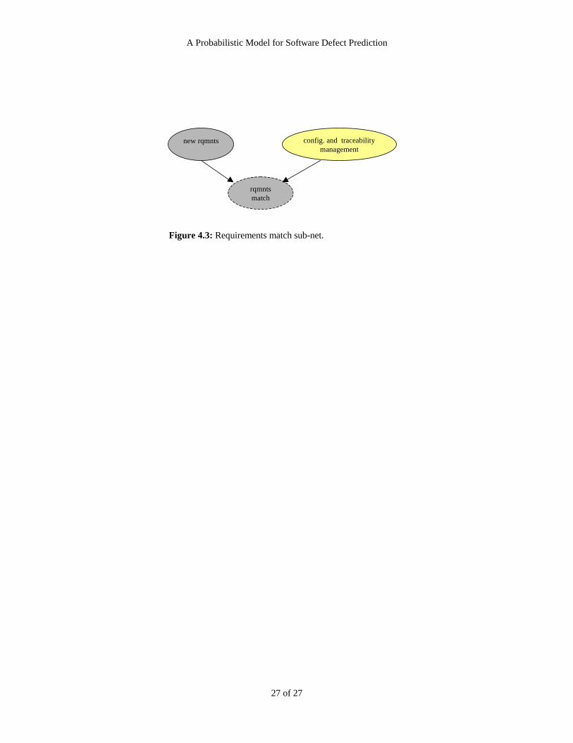
The Requirements match sub-net (Figure 4.3) contains just three nodes. These could have been

incorporated into the specification quality sub-net, but we have separated them out as a sub-net to highlight

the overall importance that we attach to the notion of requirements match. This crucial output variable

(ranging from poor to very good) represents the extent to which the implementation matches the real

requirements. It is influenced by the number of new requirements and the quality of configuration and

traceability management. When there are new requirements introduced, if the quality of configuration and

traceability management is poor then it is likely that the requirements match will be poor. This will have a

negative impact on all subsequent testing phases (hence this node is input to three other sub-nets that model

testing phases). For example, if the requirements match is poor then no matter how good the internal

development is, when it comes to the integration and independent testing phases the testers will inevitably

be testing the wrong requirements. Figure 4.3 about here.

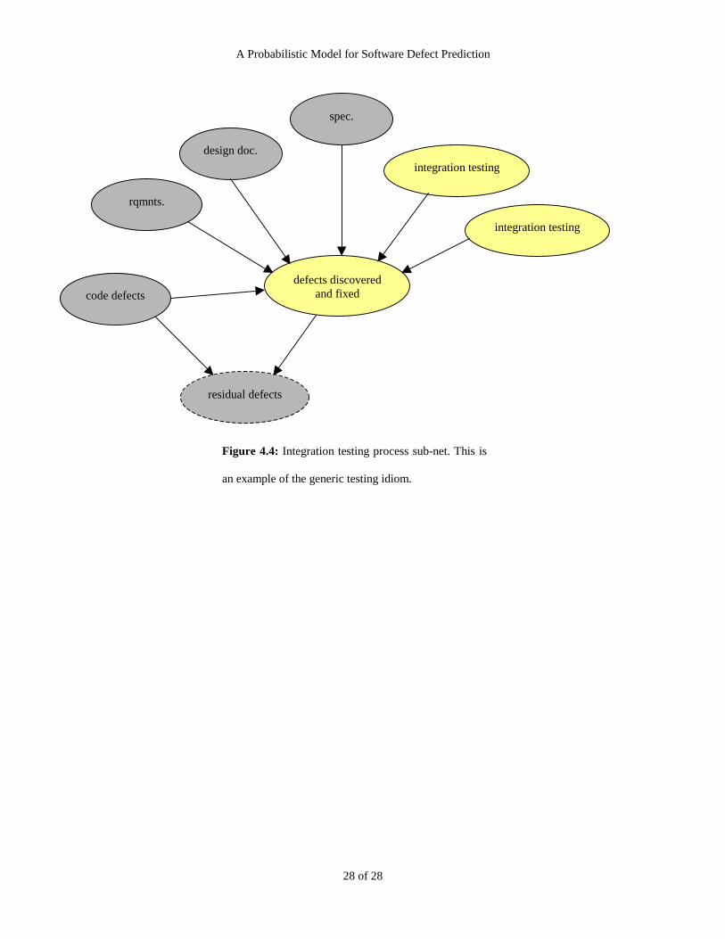
4.4 The Specification Review and Test Process sub-nets Figure 4.4 about here

The Specification Review, Unit, Integration and Independent testing process, and Operational usage sub-

nets are all based on a common testing idiom (Figure 4.4). The basic structure of each is that they receive

defects from the previous life-cycle phase as ‘inputs’, and the accuracy of testing and rework is dependent

on the resources available. The ‘output’ in each case is the unknown number of residual defects, which is

simply the number of inserted defects minus the number of discovered defects.

4.5 Design and coding process sub-net Figure 4.5 about here.

The Design and coding process sub-net (Figure 4.5) is an example of the so-called “process-product”

idiom. Based on various input resources something is being produced (namely design and code) that has

certain attributes (which are the outputs of the sub-net). The inputs here are specification quality (from the

specification quality sub-net), development staff quality and resources. These three variables define the

design and coding quality. The output attributes of the design and coding process are the design document


14 of 14

quality and the crucial number of code defects introduced. The latter is influenced not just by the quality of

the design and coding process but also by the number of residual specification defects (an input from the

specification sub-net).

4.6 Defect density sub-net

The final sub-net is the Defect density sub-net. This sub-net simply computes the industry standard defect

density metric in terms of residual defects delivered divided by module size. Notice that defect density is an

example of a node that is related to its parents by a deterministic, as opposed to a probabilistic, relationship.

This ability to incorporate deterministic nodes was an important contribution of the SERENE project.

4.7 The probability tables

The work on graphical probabilistic models outlined in Section 3 means that the problem of building such

models now factorises into two stages:

• = Qualitative stage: consider the general relationships between the variables of interest in terms of

relevance of one variable to another in specified circumstances;

• = Quantitative stage: numerical specification of the parameters of the model.

The numerical specification of the parameters means building Node Probability Tables (NPTs) for each of

the nodes in the network. However, although the problem of eliciting tables on a node by node basis is

cognitively easier that eliciting global distributions, the sheer number of parameters to be elicited remains a

very serious handicap to the successful building of probabilistic models. We will outline some of the

techniques we used to handle this problem in this sub-section.

Note that for reasons of commercial sensitivity, the parameter values used in this paper may not correspond

to the actual values used.

The leaf nodes (those with no parents) are the easiest to deal with since we can elicit the associated

marginal probabilities from the expert simply by asking about frequencies of the individual states. For

example, consider the leaf node novelty in Figure 4.2. This node has five states “very high”, “high”,

“average”, “low”, “very low”. Suppose the expert judgement is that modules typically are not very novel,

giving the following weights (as surrogates for the probability distribution), respectively, on the basis of

knowledge of all previous modules in a development organisation: 5,10,20,40,20.


15 of 15

These are turned into probabilities 0.05, 0.11, 0.21, 0.42, 0.21 (note the slight change of scale to normalise

the distribution).

The NPTs for all other leaf nodes were determined in a similar manner (by either eliciting weightings or a

drawing of the shape of the marginal distribution).

The NPTs for nodes with parents are much more difficult to define because, for each possible value that the

node can take, we have to provide the conditional probability for that value with respect to every possible

combination of values for the parent nodes. In general this cannot be done by eliciting each individual

probability – there are just too many of them (there are several million in total in this BBN). Hence we used

a variety of methods and tools that we have developed in recent projects SERENE [13] and IMPRESS [6].

For example, consider the node specification quality in Figure 4.2. This has three parent nodes resources,

intrinsic complexity, and stability each of which takes on several values (the former two have 5 values and

the latter has 4). Thus for each value for specification quality we have to define 100 probabilities. Instead

of eliciting these all directly we elicit a sample, including those at the ‘extreme’ values as well as typical,

and ask the expert to provide the rough shape of the distribution for specification quality in each case. We

then generate an actual probability distribution in each case and extrapolate distributions for all the

intermediate values. To see how this was done, Table 4.1 shows the actual data we elicited in this case. The

first three columns represent the specific sample values and the final column is the rough shape for the

distribution of “specification quality” given those values. Table 4.1 about here.

In the “best case” scenario of row 2 (resources good, stability high, complexity low) the distribution peaks

sharply close to 5 (i.e. close to “best” quality specification). If the complexity is high (row 3) then the

distribution is still skewed toward the best end, but is not as sharply peaked. In the “worst case” scenario of

row 3 (resources bad, stability low, complexity high) the distribution peaks sharply close to 1 (i.e. close to

“worst” quality specification).

On the basis of the distributions drawn by the expert we derive a function to compute the mean of the

specification quality distribution in terms of the parents variables. For example, in this case the mean used

was:

min (resource_effects, (5 * resource_effects + intrinsic_complexity + 5 * stability_effects) / 11)


16 of 16

In this example, to arrive at the distribution shapes drawn by the expert, we make use of intermediate nodes

as described in Section 4.2. For example, there is an intermediate node stability which is the parent of the

node stability effects. The stability effects node NPT is defined as the following beta distribution that is

generated using the IMPRESS tool:

Beta (2.25 * stability - 1.25, -2.25 * stability + 12.25, 1, 5)

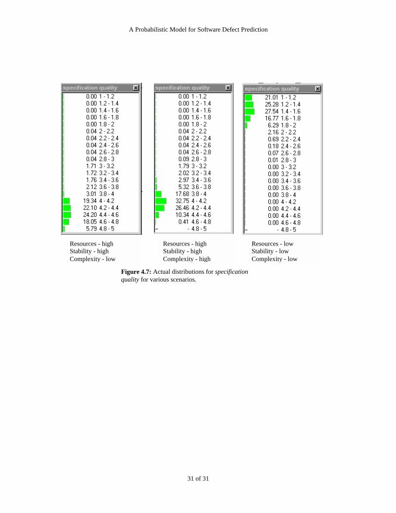
Figure 4.7 shows the actual distribution in the final BBN (using the Hugin tool) for the node specification

quality under a number of the scenarios of Table 4.1. This figure provides a good consistency check – there

is an excellent match of the distributions with those specified by the expert. Figure 4.7 about here.

4.8 Some comments on the basic probabilistic network

The methods used to construct the model have been illustrated in this section. The resulting network

models the entire development and testing life-cycle of a typical software module. We believe it contains

all the critical causal factors at an appropriate level of granularity, at least within the context of software

development within Philips.

The node probability tables (NPTs) were built by eliciting probability distributions based on experience

from within Philips. Some of these were based on historical records, others on subjective judgements. For

most of the non-leaf nodes of the network the NPTs were too large to elicit all of the relevant probability

distributions using expert judgement. Hence we used the novel techniques, that have been developed

recently on the SERENE and IMPRESS projects, to extrapolate all the distributions based on a small

number of samples. By applying numerous consistency checks we believe that the resulting NPTs are a fair

representation of experience within Philips.

As it stands, the network can be used to provide a range of predictions and “what-if” analyses at any stage

during software development and testing. It can be used both for quality control and process improvement.

However, two further areas of work were needed before the tool could be considered ready for extended

trials. Firstly and most importantly, the network needed to be validated using real-world data. Secondly a

more user-friendly interface needed to be engineered so that (a) the tool did not require users to have

experience with probabilistic modelling techniques, and (b) a wider range of reporting functions could be


17 of 17

provided. The validation exercise will be described in the next section in a way that illustrates how the

probabilistic network was packaged to form the AID tool (AID for “Assess, Improve, Decide”).

5 Validation of the AID Tool

5.1 Method

The Philips Software Centre (PSC), Bangalore, India, made validation data available. We gratefully

acknowledge their support in this way. PSC is a centre for excellence for software development within

Philips, and so data was available from a wide diversity of projects from the various Business Divisions

within PSC.

Data was collected from 28 projects from three Business Divisions: Mainstream Consumer Electronics,

Philips Medical Systems and Digital Networks. This gave a spread of different sizes and types of projects.

Data was collected from three sources:

• = Pre-release and post-release defect data was collected from the “Performance Indicators” database.

• = More extensive project data was available from the Project Database.

• = Completed questionnaires on selected projects.

In addition, the network was demonstrated in detail on a one to one basis to three experienced quality/test

engineers to obtain their reaction to its behaviour under a number of hypothetical scenarios.

The data from each project was entered into the probabilistic model. For each project:

1. The data available for all nodes prior to the Unit Test sub-net was entered first.

2. Available data for the Unit Test sub-net was then entered, with the exception of data for defects

discovered and fixed.

3. If pre-release defect data was available, the predicted probability distribution for defects detected and

fixed in the unit test phase was compared with the actual number of pre-release defects. No distinction

was made between major and minor defects – total numbers were used throughout. The actual value

for pre-release defects was then entered.


18 of 18

4. All further data for the test phases was then entered where available, with the exception of the number

of defects found and fixed during independent testing (“post-release defects”). The predicted

probability distribution for defects found and fixed in independent testing was compared with the

actual value.

5. If available, the actual value for the number of defects found and fixed during independent testing was

then entered. The prediction for the number of residual defects was then noted.

Unfortunately, data was not available to validate the operational usage sub-net. This will need data on field

call-rates that is not currently available.

Given the size of the probabilistic network, this was insufficient data to perform rigorous statistical tests of

validity. However, it was sufficient data to be able to confirm whether or not the network’s predictions

were reliable enough to warrant recommending that a more extensive controlled trial be set up.

5.2 Summary of results of the validation exercise

Overall there was a high degree of consistency between the behaviour of the network and the data that was

collected. However, a significant amount of data is needed in order to make reasonably precise predictions

for a specific project. Extensive data (filled questionnaire, plus project data, plus defect data) was available

for seven of the 28 projects. These seven projects showed a similar degree of consistency to the project that

will be studied in the next sub-section. The remaining 21 projects show similar effects, but as the

probability distributions are broader (and hence less precise) given the significant amounts of “missing”

information, the results are supportive but less convincing than the seven studied in detail.

It must be emphasised that all defect data refers to the total of major and minor defects. Hence, residual

defects may not result in a “failure” that is perceptible to a user. This is particularly the case for user-

interface projects.

Note also that the detailed contents of the questionnaires are held in confidence. Hence we cannot publish

an example of data entry for the early phases in the software life cycle. Defect data will be reported here,

but we must keep the details of the project anonymous.


19 of 19

5.3 An example run of AID

We will use screen shots of the AID Tool to illustrate both the questionnaire based user interface, and a

typical validation run.

One of the concerns with the original network is that many of the nodes have values on a simple ordinal

scale, range from “very good” to “very poor”. This leaves open the possibility that different users will

apply different calibrations to these scales. Hence the reliability of the predictions may vary, dependent on

the specific user of the system. We address this by providing a questionnaire based front-end for the

system. The ordinal values are then associated with specific question answers. The answers themselves are

phrased as categorical, non-judgemental statements. Figure 5.1 about here.

The screen in Figure 5.1 shows the entire network. The network is modularised so that a Windows Explorer

style view can be used to navigate quickly around the network. Check-boxes are provided to indicate which

questions have already been answered for a specific project.

The questions associated with a specific sub-net can then be displayed. A question is answered by selecting

the alternative from the suggested answers that best matches the state of current project. Figure 5.2 shows

the question and alternative answers for the Configuration and Traceability Management node in the

Requirements Control sub-network. Figure 5.2 about here,

For this example project, answers were available for 13 of the 16 questions preceding “defects discovered

and fixed during unit test”. Once the answers to these questions were entered, the predicted probability

distribution for defects discovered and fixed during unit test had a mean of 149 and median of 125 (see

Figure 5.3 – in this figure the monitor window has been displayed in order to show the complete probability

distribution for this prediction. Summary statistics can also be displayed.). The actual value was 122. Given

that the probability distribution is skewed, the median is the most appropriate summary statistic, so we

actually see an apparently very close agreement between predicted and actual values. This agreement was

very surprising as although we were optimistic that the “qualitative behaviour” of the network to be

transferable from organisation to organisation, we were expecting the scaling of the defect numbers to vary.

Note, however, that the median is an imprecise estimate of the number of defects – it is the centre value of


20 of 20

its associated bin on the histogram. So it might be more appropriate to quote a median of “100-150” in

order to make the imprecision of the estimate explicit. Figure 5.3 about here.

The actual value for defects discovered and fixed was entered. Answers for “staff quality” and “resources”

were available for the Integration Test and Independent Test sub-networks. Once these had been entered,

the prediction for defects discovered and fixed during independent test had a mean of 51, median of 30 and

standard deviation of 45. The actual value was 31.

As was the case with unit test, there was close agreement between the median of the prediction and the

actual value. “Test 3” was developed by PSC as a module or sub-system for a specific Philips development

group. The latter then integrated “Test 3” into their product, and tested the complete product. This is the

test phase we refer to as Independent Test.

The code size of Test 3 was 144 KLOC. The modules (perhaps sub-system is a better term given the size)

used in the validation study ranged in size from 40-150 KLOC. The probabilistic reliability model

incorporates a relatively weak coupling between module size and numbers of defects. The results of the

validation continue to support the view that other product and process factors have a more significant

impact on numbers of defects. However, we did make one modification to the specification quality sub-net

as a result of the experience gained during the validation. Instead of “Intrinsic Complexity” being the sole

direct influence on “Module Size”, we have now explicitly factored out “Problem Size” as a joint influence

with “Intrinsic Complexity” on “Module Size”.

5.4 Conclusions

A disadvantage of a reliability model of this complexity is the amount of data that is needed to support a

statistically significant validation study. As the metrics programme at PSC is relatively young (as is the

organisation itself), this amount of data was not available. As a result, we were only able to carry out a less

formal validation study. Nevertheless, the outcome of this study was very positive. Feedback was obtained

on various aspects of the functionality provided by the AID interface to the reliability model, yet the results

indicated that only minor changes were needed to the underlying model itself. We are now preparing for a

more extended trial using a wider range of projects. This should begin in the early part of 2001.


21 of 21

There is a limit to what we can realistically expect to achieve in the way of statistical validation. This is

inherent in the nature of software engineering. Even if a development organisation conforms to well

defined processes, they will not produce homogenous products – each project will differ to an extent.

Neither do we have the large relevant sample sizes necessary for statistical process control. It is primarily

for these reasons that we augment empirical evidence with expert judgement using the Bayesian framework

described in this paper. As more data becomes available, it is possible to critique and revise the model so

that the probability tables move from being subjective estimates to being a statement of physical properties

of the world (see, e.g. [7]). However, in the absence of an extensive and expensive reliability testing phase,

this model can be used to provide an estimate of residual defects that is sufficiently precise for many

software project decisions.

6 Summary

We have described a probabilistic model for software defect prediction. This model can not only be used

for assessing ongoing projects, but also for exploring the possible effects of a range of software process

improvement activities. If costs can be associated with process improvements, and benefits assessed for the

predicted improvement in software quality, then the model can be used to support sound decision making

for SPI (Software Process Improvement). The model performed very well in our preliminary validation

experiments. In addition, a user interface has been developed for the tool that enables it to be easily used in

a variety of different modes for product assessment and SPI. Although we anticipate that the model will

need additional refinement as experience is gained during extended trials, we are confident that it will make

a significant contribution to sound and effective decision making in software development organisations.

7 Acknowledgements

Simon Forey carried out the user interface development for AID; his contribution to this project was

invaluable. We would also like to thank Mr. S. Nagarajan, Mr. Thangamani N., Mr. Soumitra Lahiri, Mr.

Jitendra Shreemali and all the others at PSC, Bangalore who helped in the validation study. The validation

study was started with Mainstream CE projects at PSC, with valuable support from the Software Quality

Engineering Team in this division.


22 of 22

8 Figures

S D

Figure 2.1: Two alternative models of in influence between some predictor S (typically a size measure),

and the number of software defects D. (a) is a graphical representation of a naïve regression model. In (b)

the influence of S on D is now mediated through a common cause PS. This model can behave in the same

way as that of (a), but only in certain specific circumstances.

S D

PC

(a) (b)


23 of 23

TE SQ

DD

Figure 3.1: Some subtle interactions between variables captured in a simple

graphical model. Node TE represents “Test Effectiveness”, SQ represents

“Software Quality” and DD represents “Defects Detected and Fixed”.


24 of 24

Figure 3.2: X is conditionally independent of Y given Z.

X

Z

Y


25 of 25

Specificationquality

Specificationreview

Requirementsmatch

Design and codingprocess

Unit testing process

Independenttesting process

Defect density

Operational usage

Specificationdefects

Residualspecification

defects

Newrequirements

Code defectsDesign doc quality

Residualdefects

Residualdefects

delivered

Module sizeSpec quality

Matchingrequirements

Intrinsiccomplexity

Integration testingprocess

Residualdefects

Design docquality

Figure 4.1: Overall network structure.


26 of 26

Figure 4.2: Specification quality sub-net.

internal resources

specification quality

schedule staff quality

document quality

stakeholder involvement

novelty

intrinsic complexity

stability

new rqmnts effects

module size

spec. defects new

rqmnts


27 of 27

new rqmnts

rqmntsmatch

config. and traceabilitymanagement

Figure 4.3: Requirements match sub-net.


28 of 28

integration testing

residual defects

defects discovered and fixed code defects

rqmnts.

design doc.

spec.

integration testing

Figure 4.4: Integration testing process sub-net. This is

an example of the generic testing idiom.


29 of 29

code defectsintroduced design doc.

quality

residual spec.defects

specificationquality

developmentstaff quality

resourcesdesign andcoding quality

Figure 4.5: Design and coding process sub-net – an example of the“process-product” idiom.


30 of 30

Resources

(1 to 5 where 1 is worst 5

is best)

Stability

(1 to 3 where 1 is worst 3

is best)

Intrinsic complexity

(1 to 5 where 1 is most

complex, 5 least)

Specification quality

1 2 3 4 5

5 3 1

5 3 5

1 1 1

1 2 3

1 3 5

5 1 1

1 1 5

Table 4.1 Eliciting the probability table for specification quality.


31 of 31

Resources - highStability - highComplexity - low

Resources - lowStability - lowComplexity - low

Resources - highStability - highComplexity - high

Figure 4.7: Actual distributions for specificationquality for various scenarios.


Figure 5.1: The entire AID network illustrated using a

Windows Explorer style view.

32 of 32


33 of 33

Figure 5.2: The question associated with the

Configuration and Traceability Management node.


34 of 34

Figure 5.3: The prediction for defects discovered and fixed during Unit Test

for project “Test 3”.


35 of 35

9 References

[1] Agena Ltd, “Bayesian Belief Nets”, http://www.agena.co.uk/bbn_article/bbns.html, 1999.

[2] N.E. Fenton and S.L. Pfleeger, Software Metrics: A Rigorous and Practical Approach, (2nd Edition),

PWS Publishing Company, 1997.

[3] N. Fenton and M. Neil “A Critique of Software Defect Prediction Research”, IEEE Trans. Software

Eng., 25, No.5, 1999.

[4] N. Fenton and N. Ohlsson “Quantitative analysis of faults and failures in a complex software system”,

IEEE Trans. Software Eng., 26, 797-814, 2000.

[5] HUGIN Expert Brochure. Hugin Expert A/S, P.O. Box 8201 DK-9220 Aalborg, Denmark, 1998.

[6] IMPRESS (IMproving the software PRocESS using bayesian nets) EPSRC Project GR/L06683,

http://www.csr.city.ac.uk/csr_city/projects/impress.html, 1999.

[7] P.J. Krause. “Learning Probabilistic Networks”, Knowledge Engineering Review, 13, 321-351, 1998

[8] S.L. Lauritzen and D.J. Spiegelhalter, “Local computations with probabilities on graphical structures

and their application to expert systems” J. Roy. Stat. Soc. Ser B 50, pp. 157-224, 1988.

[9] McCall, P.K. Richards and G.F. Walters, Factors in software quality. Volumes 1, 2 and 3. Springfield

Va., NTIS, AD/A-049-014/015/055, 1977.

[10] J. Musa, Software Reliability Engineering, McGraw Hill, 1999.

[11] M. Neil, N. Fenton and L. Nielson, “Building large-scale Bayesian Networks”, Knowledge

Engineering Review, to appear 2000.

[12] J. Pearl, Probabilistic Reasoning in Intelligent Systems: Networks of Plausible Inference Morgan

Kauffman, 1988. (Revised in 1997)

[13] SERENE consortium, “SERENE (SafEty and Risk Evaluation using bayesian Nets): Method Manual”,

ESPRIT Project 22187, http://www.dcs.qmw.ac.uk/~norman /serene.htm, 1999.

http://www.csr.city.ac.uk/csr_city/projects/impress.html

a probabilistic model for software defect prediction - researchgate

Documents