a pro table sub-prime loan: obtaining the advantages of
TRANSCRIPT

A Profitable Sub-Prime Loan: Obtaining the Advantages of
Composite Order in Prime-Order Bilinear Groups
Allison Lewko∗
Columbia [email protected]
Sarah Meiklejohn†
University College [email protected]
February 5, 2015
Full version of an extended abstract published in Proceedings of PKC 2015, Springer-Verlag, 2015.Available from the IACR Cryptology ePrint Archive as Report 2013/300.
Abstract
Composite-order bilinear groups provide many structural features that are useful for both con-structing cryptographic primitives and enabling security reductions. Despite these convenient fea-tures, however, composite-order bilinear groups are less desirable than prime-order bilinear groupsfor reasons of both efficiency and security. A recent line of work has therefore focused on translatingthese structural features from the composite-order to the prime-order setting; much of this work fo-cused on two such features, projecting and canceling, in isolation, but a result due to Seo and Cheonshowed that both features can be obtained simultaneously in the prime-order setting.
In this paper, we reinterpret the construction of Seo and Cheon in the context of dual pairingvector spaces (which provide canceling as well as useful parameter hiding features) to obtain aunified framework that simulates all of these composite-order features in the prime-order setting. Wedemonstrate the strength of this framework by providing two applications: one that adds dual pairingvector spaces to the existing projection in the Boneh-Goh-Nissim encryption scheme to obtain leakageresilience, and another that adds the concept of projecting to the existing dual pairing vector spacesin an IND-CPA-secure IBE scheme to “boost” its security to IND-CCA1. Our leakage-resilient BGNapplication is of independent interest, and it is not clear how to achieve it from pure composite-ordertechniques without mixing in additional vector space tools. Both applications rely solely on theSymmetric External Diffie Hellman assumption (SXDH).
1 Introduction
Since their introduction in 2005 by Boneh, Goh, and Nissim [10], composite-order bilinear groupshave been used to construct a diverse set of advanced cryptographic primitives, including (hierarchical)identity-based encryption [30, 32], group signatures [13, 14], functional encryption [27, 29], and attribute-based encryption [31]. The main assumptions used to prove the security of such schemes are variantsof the subgroup decision assumption, which (in the simplest case) states that, for a bilinear group G oforder N = pq, without an element of order q it should be hard to distinguish a random element of Gfrom a random element of order p. Such assumptions crucially rely on the hardness of factoring N .
Beyond this basic assumption and its close variants, many of these schemes have exploited addi-tional structural properties that are inherent in composite-order bilinear groups. Two such properties,projecting and canceling, were formally identified by Freeman [19]; projecting requires (roughly) thatthere exists a trapdoor projection map from G into its p-order subgroup (and a related map in the tar-get group GT ), and canceling requires that elements in the p-order and q-order subgroups cancel each
∗Parts of this work were completed while this author was a postdoctoral researcher at Microsoft Research.†Parts of this work were completed while this author was a graduate student at UC San Diego.
1

other out (i.e., yield the identity when paired). Additionally, Lewko [28] identified another property,parameter hiding, that requires (again, roughly) that elements in the p-order subgroup reveal nothingabout seemingly correlated elements in the q-order subgroup.
While therefore quite attractive and rich from a structural standpoint, the use of composite-orderbilinear groups comes with a number of drawbacks, both in terms of efficiency and security. Until a recentconstruction of Boneh, Rubin, and Silverberg [12], all known composite-order bilinear groups were onsupersingular, or Type-1 [20], curves. Even in the prime-order setting, supersingular curves are alreadyless efficient than their ordinary counterparts: speed records for the former [4, 43] are approximatelysix times slower than speed records for the latter [5]. In the composite-order setting, it is furthermorenecessary to increase the size of the modulus by at least a factor of 10 (from 160 to at least 1024 bits) inorder to make the assumption that N is hard to factor plausible. Operations performed in composite-order bilinear groups are therefore significantly slower; for example, Guillevic [23] recently observedthat computing a pairing was 254 times slower. (This slowdown also extends to the non-supersingularconstruction of Boneh et al., and indeed to any composite-order bilinear group.) Furthermore, froma security standpoint, a number of recent results [24, 26, 22, 1, 2] demonstrate that it is possible toefficiently compute discrete logarithms in common types of supersingular curves, so that one mustbe significantly more careful when working over supersingular curves than when working over theirnon-supersingular counterparts.
One natural question to ask is: to what extent is it possible to obtain the structural advantagesof composite-order bilinear groups without the disadvantages? Although the structural properties de-scribed above might seem specific to composite-order groups, both Freeman and Lewko are in fact ableto express them rather abstractly and then describe how to construct prime-order bilinear groups inwhich each of these individual properties are met; they also show how to translate the subgroup decisionassumption into a generalized version, that in prime-order groups is implied by either Decision Linear [9]or Symmetric External Diffie Hellman (SXDH) [6]. Lewko’s approach is based on the framework of dualpairing vector spaces, as developed by Okamoto and Takashima [39, 40]. This framework has beenparticularly useful for enabling translations of cryptosystems employing the dual system encryptionmethodology in their security reductions.
In contrast, Meiklejohn, Shacham, and Freeman [37] showed that it was impossible to achieve pro-jecting and canceling simultaneously under a “natural” usage of Decision Linear; as a motivation, theypresented a blind signature scheme that seemingly relied upon both projecting and canceling for itsproof of security. Recently, Seo and Cheon [45] showed that it was actually possible to achieve bothprojecting and canceling simultaneously in prime-order groups, and Seo [44] explored both possibilityand impossibility results for projecting. To derive hardness of subgroup decision in their setting, how-ever, Seo and Cheon rely on a non-standard assumption and show that this implies the hardness ofsubgroup decision only in a very limited case. They also provide a prime-order version of the Meikle-john et al. blind signature that is somewhat divorced from their setting: rather than prove its securitydirectly using projecting and canceling, they instead alter the blind signature, introduce a new propertycalled translating, and then show that the modified blind signature is secure not in the projecting andcanceling setting, but rather in a separate projecting and translating setting.
Subsequently, Herold et al. [25] presented a new translation framework called “polynomial spaces”that achieves projecting in a natural and elegant way, and can also be augmented to simultaneouslyachieve canceling. Like the prior result of Seo and Cheon, they employ a non-standard hardness as-sumption to obtain subgroup decision hardness when projecting and canceling are both supported.Interestingly, their approach does not seem to provide a way of achieving just canceling with subgroupdecision problems relying on standard assumptions like SXDH or DLIN, as is achieved by dual pairingvector spaces. Integrating the benefits of dual pairing vector spaces into something like the polynomialspaces approach remains a worthwhile goal for future work. The framework in [25] also extends to
2

the setting of multilinear groups, as do approaches based on eigenspaces, as demonstrated for examplein [21].
Our contributions. In this paper, we present in Section 3 an abstract presentation of the projectingand canceling pairing due to Seo and Cheon [45]. Our presentation is based on dual pairing vectorspaces (DPVS) [39, 40], and it can be parameterized to yield projection properties of varying strength.This perspective yields several advantages. First, all the power of DPVS is embedded inside thisconstruction and can thus be exploited as in prior works. Second, we observe that many instances ofsubgroup decision problems in this framework are implied by the relatively simple SXDH assumption.
The advantages of our perspective are most clear for our BGN application, which we present inSection 4. If one starts with the goal of making the composite-order BGN scheme leakage resilient(i.e., providing provable security even when some bits of the secret key may have been leaked), thefirst obstacle one faces is the uniqueness of secret keys. Since the secret key is a factorization of thegroup order, there is only one secret key for each public key, making the common kind of hash proofargument for leakage resilience (as codified by Naor and Segev [38], for example) inapplicable. TheDPVS techniques baked into our projecting and canceling prime-order construction remove this barrierquite naturally by allowing secret keys to be vectors that still serve as projection maps but can now besampled from subspaces containing exponentially many potential keys. This demonstrates the benefitsof adding canceling and parameter hiding to applications that are designed around projection.
As an additional application, in Section 5, we present an IND-CCA1-secure identity-based encryp-tion (IBE) scheme that uses canceling, parameter hiding, and weak projecting properties in its proofof security. Although efficient constructions of IND-CCA2-secure IBE schemes have been previouslyobtained by combining IND-CPA-secure HIBE schemes with signatures [16], we nevertheless view ourIBE construction as a demonstration of the applicability of our unified framework. Furthermore, ournew construction does not aim to amplify security by adding new primitives; instead, it explores theexisting security of the IND-CPA-secure IBE due to Boneh and Boyen [8] (which cannot be IND-CCA2secure, as it has re-randomizable ciphertexts), and observes that, by modifying the scheme in a ratherorganic way and exploiting the (weak) projecting and canceling properties of the setting, we can proveIND-CCA1 security directly. Hence, we view this as an exploration of the security properties that canbe proved solely from the minimalistic spirit of the Boneh-Boyen scheme.
Our two applications serve as a proof of concept for the usefulness of obtaining projecting andcanceling simultaneously in the prime-order setting, and a demonstration of how to leverage such prop-erties while relying only on relatively simple assumptions like SXDH. We believe that the usefulnessof our framework extends beyond these specific examples, and we intend our work to facilitate futureapplications of these combined properties.
Our techniques. To obtain a more user-friendly interpretation of the projecting and canceling pairingconstruction over prime-order groups, we begin by observing that it is essentially a concatenation ofDPVS. Dual pairing vector spaces were first used in prime-order bilinear groups by Okamoto andTakashima [39, 40] and have since been employed in many works, in particular to instantiate dual systemtechnique [46] in the prime-order setting [29, 41, 28]. These previous uses of DPVS typically relied onthe canceling property, variants of subgroup decision problems, and certain parameter hiding propertiesthat are present by design in DPVS. One particularly nice feature of DPVS constructions is that alarge family of useful subgroup decision variants can be proven to follow from standard assumptions likeSXDH for asymmetric groups and DLIN for symmetric groups; viewing the construction of a projectingand canceling pairing as a natural extension of DPVS therefore has the twin benefits that it provides aclear guide on how to derive certain subgroup decision variants from standard assumptions, and that itcomes with all the built-in tools that DPVS offers.
3

In particular, DPVS includes a suite of vector-space-based tools for proving leakage resilience, similarto ones used in previous works [38, 15, 17, 36, 34, 18]. This enables us to combine the projecting-supported limited homomorphic functionality of the BGN encryption scheme with provable leakageresilience. DPVS also supports a toolkit developed for dual system proofs (e.g., [35, 41, 42]), which iswhat enables us to boost our IBE to full IND-CCA1 security with just the addition of projection.
2 Definitions and Notation
In this section, we define bilinear groups and the three functional properties we would like them to satisfy:projecting, canceling, and parameter hiding. For the first two, we use the definitions of Freeman [19](albeit in a somewhat modified form); for parameter hiding, on the other hand, we come up with a newformal framework. In addition to these functional properties, we consider the notion of subgroup decisionin bilinear groups, in which a random element of a subgroup should be indistinguishable from a randomelement of the full group. The variant we define, called generalized correlated subgroup decision, isvery general: in addition to seeing random elements of subgroups, we allow an attacker to see elementscorrelated across subgroups (e.g., elements of different subgroups with correlated randomness), andrequire that it is still difficult for him to distinguish between correlated elements of different subgroups.We then see in Sections 3 and 6 that many specific instances of this general notion are implied bystandard notions of subgroup decision in both prime-order and composite-order groups. that manyspecific instances of this general notion are implied by more standard notions of subgroup decision inboth prime-order and composite-order groups.
2.1 Bilinear groups
In what follows, we refer to a bilinear group as a tuple G = (N,G,H,GT , e, µ), where N is either primeor composite, |G| = |H| = kN and |GT | = `N for some k, ` ∈ N, and e : G × H → GT is a bilinearmap; i.e., e is an efficient map that satisfies both bilinearity (e(xa, yb) = e(x, y)ab for all x ∈ G, y ∈ H,a, b ∈ Z/NZ) and non-degeneracy (if e(x, y) = 1 for all x ∈ G then y = 1 and if e(x, y) = 1 for ally ∈ H then x = 1). In some bilinear groups, we may additionally include generators g and h of G andH respectively (if G and H are cyclic), information about meaningful subgroups of G and H, or someauxiliary information µ that allows for efficient membership testing in G and H (and possibly more).In what follows, we refer to the algorithm that is used to generate such a G as BilinearGen. Beyond thesecurity parameter, BilinearGen takes in an additional parameter n that specifies the number of desired
subgroups; i.e., for (N,G,H,GT , e, µ)$←− BilinearGen(1k, n), we have G = ⊕ni=1Gi and H = ⊕ni=1Hi
(where typically Gi and Hi are cyclic).In terms of functional properties of bilinear groups, we first define both projecting and canceling ;
our definitions are modified versions of the ones originally given by Freeman [19]. We give three flavorsof projecting. The first, weak projecting, considers projecting into a single subgroup of the source group,without requiring a corresponding map in the target group. The second, which we call simply projecting,most closely matches the definition given by Freeman, and considers projecting into a single subgroupin both the source and target groups. Lastly, we define full projecting, which considers projecting intoevery subgroup individually. As we will see in Section 3, we can satisfy all of these flavors by tweakingappropriate parameters in our prime-order construction.
Definition 2.1 (Weak projecting). A bilinear group G = (N,G,H,GT , e, µ) is weakly projecting ifthere exist decompositions G = G1 ⊕G2 and H = H1 ⊕H2, and projection maps πG and πH such thatπG(x1) = x1 for all x1 ∈ G1 and πG(x2) = 1 for all x2 ∈ G2, and similarly πH(y1) = y1 for all y1 ∈ H1
and πH(y2) = 1 for all y2 ∈ H2.
4

Definition 2.2 (Projecting). A bilinear group G = (N,G,H,GT , e, µ) is projecting if there existsubgroups G′ ⊂ G, H ′ ⊂ H, and G′T ⊂ GT such that there exist non-trivial maps πG : G → G′,πH : H → H ′, and πT : GT → G′T such that πT (e(x, y)) = e(πG(x), πH(y)) for all x ∈ G, y ∈ H.
Definition 2.3 (Full projecting). A bilinear group G = (N,G,H,GT , e, µ) is fully projecting if thereexists some n ∈ N and decompositions G = ⊕ni=1Gi, H = ⊕ni=1Hi, and GT = ⊕ni=1GT,i, and non-trivial maps πGi : G → Gi, πHi : H → Hi, and πT i : GT → GT,i for all i such that πT i(e(x, y)) =e(πGi(x), πHi(y)) for all x ∈ G, y ∈ H.
Definition 2.4 (Canceling). A bilinear group G = (N,G,H,GT , e, µ) is canceling if there exists somen ∈ N and decompositions G = ⊕ni=1Gi and H = ⊕ni=1Hi such that e(xi, yj) = 1 for all xi ∈ Gi, yj ∈ Hj,i 6= j.
2.2 Parameter hiding
Beyond projecting and canceling, we aim to define parameter hiding. As mentioned in the introduction,this property roughly says that elements in one subgroup should not reveal anything about relatedelements in other subgroups, and was previously used, without a formal definition, by Lewko [28]. Inessence, parameter hiding in composite-order groups is a simple consequence of the Chinese RemainderTheorem, which tells us that if we sample a random value modulo N = pq, its reductions modulo p andq are uncorrelated. In the prime-order setting, a form of parameter hiding can be instantiated from dualpairing vector spaces, leveraging the fact that if one commits to only certain parts of dual orthonormalbases over Fnp , there is remaining ambiguity in the hidden basis vectors.
The main difficulty in providing a formal definition for parameter hiding is that it is not as self-contained a feature as projecting and canceling: elements within subgroups may be related to elementsin other subgroups in a myriad of ways, and their relation to one another may depend both on the formof the element (which can involve any function on the exponents) and on the subgroups. We thereforedo not try to consider all types of correlations, but instead focus on one simple type, defined as follows:
Definition 2.5. For a bilinear group G = (N,G = ⊕ni=1Gi, H = ⊕ni=1Hi, GT , e, {gi}ni=1, {hi}ni=1), anelement x ∈ Z/NZ, and indices 1 ≤ i1, i2 ≤ n, an x-correlated sample from the subgroup Gi1 ⊕ Gi2 is
an element of the form gαi1 · gαxi2
for α$←− Z/NZ.
We also consider correlated samples in H, but for convenience we define a y-correlated sample from
the subgroup Hi1 ⊕ Hi2 to be an element of the form hβyi1 · hβi2
for β$←− Z/NZ. Although we choose
this type of correlation mainly for ease of exposition (and because we encounter it in Section 5), ourdiscussion below could be adjusted to accommodate more general types of correlation, which wouldremain compatible with our prime-order construction in Section 3.
Intuitively then, parameter hiding says that, under certain restrictions about which subgroup ele-ments one is allowed access to, the distributions over x-correlated samples and random samples shouldin fact be the same, even when x is known. (We need some restrictions because there may be testable re-lationships between the images of various generators in the target group.) To consider the distributionswe can use — i.e., what additional information we might give out besides the samples — we considerdistributions D parameterized by sets Sph
G = {SphG,gen, S
phG,sam, S
phG,cor}, S
phH = {Sph
H,gen, SphH,sam, S
phH,cor}, and
C; intuitively, SphG and Sph
H tell us which elements to include in the distribution, and C tells us whichcorrelated samples to change to random. Formally, these sets are defined as follows:
• SphG,gen indicates which subgroup generators to include: For all si ∈ Sph
G,gen, include gsi in D.
• SphG,sam is a multiset that indicates which random samples to include: For all ti = (t1,i, . . . , tmi,i) ∈SphG,sam, include a random sample from Gt1,i ⊕ . . .⊕Gtmi,i
in D.
5
• SphG,cor is a set that indicates which correlated samples to include: For all ci = (xi, c1,i, c2,i) ∈ Sph
G,cor,
include gac1,i · gaxic2,i in D, where a
$←− Z/NZ.
• SphH is defined analogously to Sph
G .
• C indicates which correlated samples to change: For all ci = (bi, c′i) ∈ C, if bi = 0 then c′i ∈ S
phG,cor
and if bi = 1 then c′i ∈ SphH,cor; i.e., we require that C ⊆ {0× Sph
G,cor} ∪ {1× SphH,cor}.
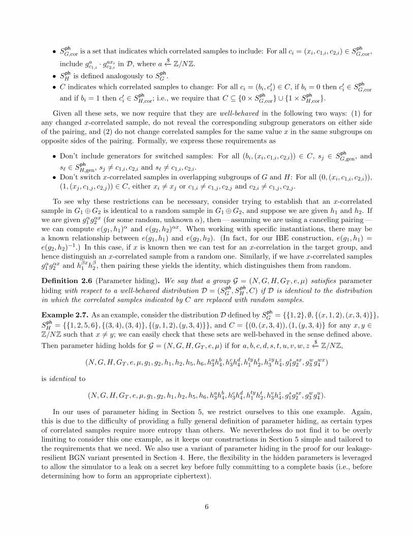
Given all these sets, we now require that they are well-behaved in the following two ways: (1) forany changed x-correlated sample, do not reveal the corresponding subgroup generators on either sideof the pairing, and (2) do not change correlated samples for the same value x in the same subgroups onopposite sides of the pairing. Formally, we express these requirements as
• Don’t include generators for switched samples: For all (bi, (xi, c1,i, c2,i)) ∈ C, sj ∈ SphG,gen, and
s` ∈ SphH,gen, sj 6= c1,i, c2,i and s` 6= c1,i, c2,i.
• Don’t switch x-correlated samples in overlapping subgroups of G and H: For all (0, (xi, c1,i, c2,i)),(1, (xj , c1,j , c2,j)) ∈ C, either xi 6= xj or c1,i 6= c1,j , c2,j and c2,i 6= c1,j , c2,j .
To see why these restrictions can be necessary, consider trying to establish that an x-correlatedsample in G1 ⊕G2 is identical to a random sample in G1 ⊕G2, and suppose we are given h1 and h2. Ifwe are given gα1 g
αx2 (for some random, unknown α), then — assuming we are using a canceling pairing —
we can compute e(g1, h1)α and e(g2, h2)
αx. When working with specific instantiations, there may bea known relationship between e(g1, h1) and e(g2, h2). (In fact, for our IBE construction, e(g1, h1) =e(g2, h2)
−1.) In this case, if x is known then we can test for an x-correlation in the target group, andhence distinguish an x-correlated sample from a random one. Similarly, if we have x-correlated samplesgα1 g
αx2 and hβx1 hβ2 , then pairing these yields the identity, which distinguishes them from random.
Definition 2.6 (Parameter hiding). We say that a group G = (N,G,H,GT , e, µ) satisfies parameter
hiding with respect to a well-behaved distribution D = (SphG , S
phH , C) if D is identical to the distribution
in which the correlated samples indicated by C are replaced with random samples.
Example 2.7. As an example, consider the distribution D defined by SphG = {{1, 2}, ∅, {(x, 1, 2), (x, 3, 4)}},
SphH = {{1, 2, 5, 6}, {(3, 4), (3, 4)}, {(y, 1, 2), (y, 3, 4)}}, and C = {(0, (x, 3, 4)), (1, (y, 3, 4)} for any x, y ∈
Z/NZ such that x 6= y; we can easily check that these sets are well-behaved in the sense defined above.
Then parameter hiding holds for G = (N,G,H,GT , e, µ) if for a, b, c, d, s, t, u, v, w, z$←− Z/NZ,
(N,G,H,GT , e, µ, g1, g2, h1, h2, h5, h6, ha3h
b4, h
c3hd4, h
ty1 h
t2, h
zy3 h
z4, g
s1gsx2 , g
w3 g
wx4 )
is identical to
(N,G,H,GT , e, µ, g1, g2, h1, h2, h5, h6, ha3h
b4, h
c3hd4, h
ty1 h
t2, h
v3h
z4, g
s1gsx2 , g
w3 g
u4 ).
In our uses of parameter hiding in Section 5, we restrict ourselves to this one example. Again,this is due to the difficulty of providing a fully general definition of parameter hiding, as certain typesof correlated samples require more entropy than others. We nevertheless do not find it to be overlylimiting to consider this one example, as it keeps our constructions in Section 5 simple and tailored tothe requirements that we need. We also use a variant of parameter hiding in the proof for our leakage-resilient BGN variant presented in Section 4. Here, the flexibility in the hidden parameters is leveragedto allow the simulator to a leak on a secret key before fully committing to a complete basis (i.e., beforedetermining how to form an appropriate ciphertext).
6

2.3 Generalized correlated subgroup decision
Beyond functional properties of bilinear groups, we must also consider the types of security guar-antees we can provide. The assumption we define, generalized correlated subgroup decision, consid-ers indistinguishability between subgroups in a very general way: given certain subgroup generatorsand “correlated” elements across subgroups (i.e., elements in different subgroups that use the samerandomness), it should still be hard to distinguish between elements of other subgroups. Formally,
we consider sets SsghG = {Ssgh
G,gen, SsghG,sam}, S
sghH = {Ssgh
H,gen, SsghH,sam}, T1 = {(`1, λ1), . . . , (`m, λm)}, and
T2 = {(`′1, λ′1), . . . , (`′m+1, λ′m+1)}, and an indicator bit b. (We assume without loss of generality that
T2 is the larger set.) Intuitively, SsghG and Ssgh
H tell us which group elements an adversary is given, and(T1, T2, b) tell us what the challenge terms should look like. We have the following requirements:
• SsghG,gen indicates which subgroup generators to include: Give out gsi for all si ∈ Ssgh
G,gen.
• SsghG,sam indicates which samples to include: For each
ti = ((`1,i, λ1,i), . . . , (`mi,i, λmi,i)) ∈ SsghG,sam
, give out ga1`1,i · . . . · gami`mi,i
and ga1λ1,i · . . . · gamiλmi,i
for a1, . . . , ami
$←− Z/NZ. These elements are
correlated, in that the same randomness is used for both.
• The bit b indicates which group the challenge element comes from: b = 0 indicates G, and b = 1indicates H.
• The sets T1 and T2 must differ in exactly one pair; i.e., there must exist a unique pair P suchthat P /∈ T1 but P ∈ T2. For this pair P = (`, λ), we cannot give out the subgroup generators on
either side of the pairing, so we require si 6= ` and si 6= λ for any si ∈ SsghG,gen or si ∈ Ssgh
H,gen.
If P ∈ ti for some ti ∈ SsghG,sam∪S
sghH,sam, then T1∩ ti 6= ∅; i.e., P can appear only in random samples
that also contain another component in the challenge term. Then, assuming b = 0 (and replacingg with h if b = 1), our challenge elements are of the form T := (ga1`1 · . . . · g
am`m, ga1λ1 · . . . · g
amλm
) and
T ′ := (ga1`1′· . . . · gam+1
`′m+1, ga1λ′1
· . . . · gam+1
λ′m+1) for a1, . . . am+1
$←− Z/NZ.
Assumption 2.8 (Generalized correlated subgroup decision). For all tuples (SsghG , Ssgh
H , T1, T2, b) sat-
isfying the requirements specified above and for any n ∈ N, for any PPT adversary A given G $←−BilinearGen(1k, n) and the elements specified by Ssgh
G and SsghH , it is hard to distinguish between values
T defined by (b, T1) and values T ′ defined by (b, T2).
As an example, consider the case in which n = 6 and SsghG = {{1, 2}, {((1, 2), (3, 4))}}, Ssgh
H ={{1, 2, 5, 6}, {((1, 2), (3, 4)), ((3, 4), (5, 6))}}, T1 = {(1, 2), (5, 6)}, T2 = {(1, 2), (3, 4), (5, 6)}, and b = 0.In this case, the concrete assumption is: Given G and generators g1, g2, h1, h2, h5, h6, correlated samplesfrom G1⊕G3 and G2⊕G4, correlated samples from H1⊕H3 and H2⊕H4, and correlated samples fromH3 ⊕H5 and H4 ⊕H6, it should be hard to distinguish correlated samples from G1 ⊕G5 and G2 ⊕G6
from correlated samples from G1 ⊕G3 ⊕G5 and G2 ⊕G4 ⊕G6.
3 A Prime-Order Bilinear Group Satisfying All Features
Our ultimate goal in this section is to define a prime-order bilinear group that satisfies all three of theproperties defined in the previous section: projecting, canceling, and parameter hiding; additionally, wewant to require that subgroup decision is hard in this group. Our construction can be viewed as anabstraction of the construction of Seo and Cheon [45], which they prove satisfies (regular) projecting,
7

canceling, and a somewhat restrictive notion of subgroup decision. In contrast, our construction satisfiescanceling and parameter hiding, is flexible enough to achieve any of the three flavors of projectingwe defined in the previous section (depending on the parameter choices), and comes equipped withreductions for more general instances of subgroup decision.
Notationally, we augment the bilinear groups G discussed in the previous section: we now focusonly on the case when the group order is some prime p, and consider G = (p,B1, B2, BT , E, µ) built ontop of G = (p,G,H,GT , e); this means B1, B2, and BT may contain multiple copies of G, H, and GTrespectively, and that the map E uses e as a component. Because we are moving to bigger spaces, we alsoinclude a value µ that allows us to test membership in B1 and B2; as an example, consider B1 ⊂ G×G.Then, while an efficient membership test for G implies one for G×G, additional information µ may benecessary to allow one to (efficiently) test for membership in B1.
Our construction crucially uses dual pairing vector spaces, which were introduced by Okamoto andTakashima [39, 40] and have been previously used to provide pairings E : Gn ×Hn → GT , built on topof pairings e : G×H → GT , that satisfy the canceling property. As we cannot have a cyclic target spaceif we want to satisfy projecting, however, we instead need a map whose image is GdT for some d > 1.Intuitively, we achieve this by piecing together d “blocks,” where each block is an instance of a dualpairing vector space; the construction of Seo and Cheon is then obtained as the special case in whichd = n, and regular dual pairing vector spaces are obtained with d = 1. We begin with a key definition:
Definition 3.1 (Dual orthonormal). Two bases B = (~b1, . . . ,~bn) and B∗ = (~b∗1, . . . ,~b∗n) of Fnp are dual
orthonormal if ~bj ·~b∗j ≡ 1 mod p for all j, 1 ≤ j ≤ n, and ~bj ·~b∗k ≡ 0 mod p for all j 6= k.
We note that one can efficiently sample a random pair of dual orthonormal bases (B,B∗) by samplingfirst a random basis B and then solving uniquely for B∗ using linear algebra over Fp; we denote this
sampling process as (B,B∗) $←− Dual(Fnp ). By repeating this sampling process d times, we can obtain atuple ((B1,B∗1), . . . , (Bd,B∗d)) of d pairs of dual orthonormal bases of Fnp . We denote the vectors of Bi as
(~b1,i . . . ,~bn,i), and the vectors of B∗i as (~b∗1,i, . . . ,~b∗n,i). We then give the following definition:
Definition 3.2 (Concatenation). The concatenation of bases (B1, . . . ,Bd) of Fnp is a collection of n
vectors (~v1, . . . , ~vn) in Fdnp , where each ~vj := ~bj,1|| . . . ||~bj,d. Alternatively, we can view each ~vj as a d×nmatrix, where the i-th row is ~bj,i. We denote the concatenation of (B1, . . . ,Bd) as Concat(B1, . . . ,Bd).
To begin our construction, we build off G = (p,G,H,GT , e, g, h), where g and h are generators of Gand H respectively, and consider groups B1 ⊂ Gdn and B2 ⊂ Hdn. Notationally, we write an element ofB1 as gA, where A = (αi,j)
d,ni,j=1 is a d× n matrix and gA := (gα1,1 , . . . , gα1,j , . . . , gα1,n , gα2,1 , . . . , gαd,n).
We similarly write elements of B2 as hB for a d× n matrix B = (βij)d,ni,j=1, and furthermore define the
bilinear map E : B1 ×B2 → GdT as
E(gA, hB) :=
(n∏k=1
e(gα1,k , hβ1,k), . . . ,n∏k=1
e(gαd,k , hβd,k)
). (1)
Observe that the i-th coordinate of the image is equal to e(g, h)Ai·Bi mod p, where Ai and Bi denote thei-th rows of A and B respectively. Then, to begin to see how our construction will satisfy projectingand canceling, we have the following lemma:
Lemma 3.3. Let (~v1, . . . , ~vn) = Concat(B1, . . . ,Bd) and (~v∗1, . . . , ~v∗n) = Concat(B∗1, . . . ,B∗d), where
(Bi,B∗i ) are dual orthonormal bases of Fnp . Then
E(g~vj , h~v∗j ) = (e(g, h), . . . , e(g, h)) ∀j and E(g~vj , h~v
∗k) = (1T , . . . , 1T ) ∀j 6= k.
8

Proof. By definition of the pairing,
E(g ~vj , h~v∗k) =
(e(g, h)
~bj,1·~b∗k,1 , . . . , e(g, h)~bj,d·~b∗k,d
)for any j and k. If j = k, then the fact that (Bi,B∗i ) are dual orthonormal for all i implies by definition
that ~bj,i · ~b∗j,i ≡ 1 mod p for all i and j, and thus E(g~vj , h~v∗j ) = (e(g, h), . . . , e(g, h)). For the second
property, we again use the definition of dual orthonormal bases to see that ~bj,i ·~b∗k,i ≡ 0 mod p for all
j 6= k, and thus E(g~vj , h~v∗k) = (1T , . . . , 1T ).
While Lemma 3.3 therefore shows us directly how to obtain canceling, for projecting we are stillmapping into a one-dimensional image. To obtain more dimensions, it turns out we need only performsome additional scalar multiplication. We give the following definition:
Definition 3.4 (Scaling). Define C = (ci,j)d,ni,j=1 to be a n × d matrix of entries over Fp \ {0}. Given
bases (B1, . . . ,Bd) of Fnp , we define the scaling of these bases by C to be new bases (D1, . . . ,Dd),where Di = (c1,i~b1,i, . . . , cn,i~bn,i) for all i, 1 ≤ i ≤ d. We denote the scaling of (B1, . . . ,Bd) by Cas Scale(C,B1, . . . ,Bd).
Intuitively then, we use the entries in the i-th column of C to scale the vectors in the basis Bi andobtain the basis Di. As we still have ~bj,i ·~b∗k,i ≡ 0 mod p for j 6= k, multiplication by a scalar will notaffect this and we still satisfy canceling. The scalar values do, however, build in extra dimensions intothe image of our pairing, as demonstrated by the following lemma:
Lemma 3.5. Let (B1, . . . ,Bd) and (B∗1, . . . ,B∗d) be sets of bases for Fnp such that (Bi,B∗i ) are dualorthonormal for all i. Define (~v1, . . . , ~vn) := Concat(D1, . . . ,Dd) and (~v∗1, . . . , ~v
∗n) := Concat(B∗1, . . . ,B∗d),
where (D1, . . . ,Dd) = Scale(C,B1, . . . ,Bd) for some C ∈Mn×d(Fp). Then
E(g~vj , h~v∗j ) = (e(g, h)cj,1 , . . . , e(g, h)cj,d) ∀j and
E(g~vj , h~v∗k) = (1T , . . . , 1T ) ∀j 6= k.
Proof. By definition of the pairing,
E(g~vj , h~v∗k) =
(e(g, h)cj,1
~bj,1·~b∗k,1 , . . . , e(g, h)cj,d~bj,d·~b∗k,d
)for any j and k. If j = k, then the fact that (Bi,B∗i ) are dual orthonormal for all i implies by
definition that ~bj,i ·~b∗j,i ≡ 1 mod p for all i and j, and thus cj,i~bj,i ·~b∗j,i ≡ cj,i mod p and E(g~vj , h~v∗j ) =
(e(g, h)cj,1 , . . . , e(g, h)cj,d). For the second property, we again use the definition of dual orthonormalbases to see that ~bj,i ·~b∗k,i ≡ 0 mod p for all j 6= k, and thus cj,i~bj,i ·~b∗k,i ≡ 0 mod p and E(g~vj , h~v
∗k) =
(1T , . . . , 1T ).
We are now ready to give our full construction of an algorithm BilinearGen′, parameterized by integersn and d, and a distribution Dn,d on n× d matrices, to achieve a setting G = (p,B1, B2, BT , E, µ) suchthat B1 ⊂ Gdn, B2 ⊂ Hdn, and BT = GdT . We present this construction in Algorithm 1, and demonstratethat it satisfies projecting, canceling, parameter hiding, and subgroup decision.
The generality of this construction stems from the choices of d, n, and D; in fact, by choosingdifferent values for these parameters, we can satisfy each of the different flavors of projecting fromSection 2. To satisfy fully projecting, we choose C from a distribution over matrices of full rank n anduse d ≥ n. If we use a less restrictive distribution, we obtain weaker projection capabilities and a moreefficient construction (as we can have d < n) when projecting onto all subgroups individually is notneeded: to achieve (regular) projecting, we can use d > 1 and pick C to be of rank > 1, and to achieveweak projecting we can in fact use d = 1 and pick C to be the vector consisting of all 1 entries. (Thislast case is equivalent to working in regular dual pairing vector spaces.)
9

Algorithm 1 BilinearGen′: generate a bilinear group G that satisfies projecting and canceling
Input: d, n ∈ N; distribution Dd,n over matrices in Mn×d(Fp); security parameter 1k.
1. (p,G,H,GT , e)$←− BilinearGen(1k, 1).
2. Pick values g and h such that G = 〈g〉 and H = 〈h〉.3. Sample d pairs (Bi,B∗i )
$←− Dual(Fnp ) to obtain two sets (B1, . . . ,Bd) and (B∗1, . . . ,B∗d) of bases ofFnp , where (Bi,B∗i ) are dual orthonormal.
4. Sample C = (cij)d,ni,j=1
$←− D and compute (D1, . . . ,Dd) := Scale(C,B1, . . . ,Bd).5. For all i, 1 ≤ i ≤ n, define B1,i := 〈g~vi〉 and B2,i := 〈h~v∗i 〉, where (~v1, . . . , ~vn) := Concat(D1, . . . ,Dd)and (~v∗1, . . . , ~v
∗n) := Concat(B∗1, . . . ,B∗d).
6. Define B1 := ⊕ni=1B1,i ⊂ Gdn, B2 := ⊕ni=1B2,i ⊂ Hdn, and BT := GdT . Define the pairingE : B1 ×B2 → BT as in Equation 1.7. Finally, to be able to check that an element gM ∈ Gdn for M = (mij)
d,ni,j=1 is an element of B1, we
observe that the vectors ~v1, . . . , ~vn span an n-dimensional subspace V of Fdnp . Thus, there must beanother subspace, call it W, of dimension dn−n, that contains all vectors in Fnp that are orthogonal to
vectors in V. Given µ2 := (h~w1 , . . . , h~w(d−1)n), where the {~wi}(d−1)ni=1 are a basis of W, one can thereforeefficiently check if gM ∈ B1 by checking if E(gM , h~wi) = (1T , . . . , 1T ) for all i, 1 ≤ i ≤ (d− 1)n.
Analogously, given µ1 := (g ~w∗1 , . . . , g
~w∗(d−1)n), one can check if hA ∈ B2 by checking if E(g ~w
∗i , hA) =
(1T , . . . , 1T ), where {~w∗i }(d−1)ni=1 are a basis for the subspace W∗ of Fnp consisting of vectors orthogonal
to vectors in the span of ~v∗1, . . . , ~v∗n.
8. Output G := (p,B1, B2, BT , E, (µ1, µ2)).
Theorem 3.6. For all values of n ≥ 2, the bilinear group G $←− BilinearGen′(1k, n, d,Dd,n) satisfiescanceling, fully projecting as defined in Definition 2.3 for d ≥ n when Dd,n is defined over full-rankmatrices, projecting as defined in Definition 2.2 for d > 1 when Dd,n is defined over matrices of rank> 1, and weak projecting as defined in Definition 2.1 for d = 1.
Proof. Given that our construction was specifically designed to satisfy the conditions for Lemma 3.5, weimmediately obtain canceling. To satisfy projecting, we additionally need to construct the projectionmaps πij and argue that they satisfy the requirements of Definition 2.3 (in the case that C is full rank).By the way our subgroups are defined, each projection map π1i within the group B1 must map anarbitrary element ga1~v1+···+an~vn of B1 to gai ~vi ∈ B1,i; similarly, π2i must map ha
∗1~v∗1+···+a
∗n~v∗n ∈ B2 to
ha∗i ~v∗i ∈ B2,i. For π1i, we observe that it can be computed efficiently by anyone knowing ~vi and another
vector in Fdnp that is orthogonal to ~vk for all k 6= i. The situation for π2i is analogous.As for the projection maps πT,i required for the target space, we define πT,i to map an element
e(g, h)a1C1+···+anCn to e(g, h)aiCi , where we recall Ci denotes the i-th row of the scaling matrix C (Ciis thus a vector in Fdp for all i).
Finally, we show that the required associativity property holds, namely that E(π1,i(gM ), π2,i(h
A)) =πT,i(E(gM , hA)) for all elements gM ∈ B1, h
A ∈ B2, and for all i, 1 ≤ i ≤ d. To see this, observethat gM ∈ B1 implies that gM = gα1~v1+···+αn~vn for some α1, . . . , αn ∈ Fp, and similarly that hA =hβ1~v
∗1+···+βn~v
∗n . We therefore have that
E(π1,i(gM ), π2,i(h
A)) = E(gαi~vi , hβi~v∗i ) = e(g, h)αiβiCi ,
where this last equality follows from Lemma 3.5. On the other hand, we have that
πT,i(E(gM , hA)) = πT,i(n∏k=1
e(g, h)αkβkCk) = e(g, h)αiβiCi ,
10

and the two quantities are therefore equal.A similar argument applies to obtaining more limited projections when C has lower rank.
It remains to prove that our construction also satisfies parameter hiding and subgroup hiding.For the latter property, our definition in Section 2.3 is highly general and we cannot prove that allinstances of generalized correlated subgroup decision reduce to any one assumption. Instead, we showthat certain “nice” instances of the assumption follow from SXDH.
Before we define a nice instance, we first restrict our attention to the case where n = 8, d = 1,C is a matrix with all 1 entries. For succinctness here and in later sections, we use BasicGen(1k) =BilinearGen′(1k, 8, 1,D), where D produces matrices with all 1 entries; i.e., we use BasicGen to producethe specific setting in which we are interested in Section 5.
We consider two variants of this setting, which differ only in the auxiliary information µ. For µ asdefined above in Algorithm 1, we show that the required instances of the correlated subgroup decisionassumption are implied by SXDH. We additionally consider a case where µ is augmented to contain thefollowing three pieces of information: (1) the vectors ~v7, ~v8, ~v
∗7, and ~v∗8; (2) a random basis for the span
of (~v1, . . . , ~v6) inside F8p; and (3) a random basis for the span of (~v∗1, . . . , ~v
∗6) inside F8
p. With this µ, one
can then perform a membership test for G1 ⊕ . . . ⊕ G6 on some element g~v by computing a basis forthe orthogonal space of the span of (~v1, . . . , ~v6), pairing against h raised to these vectors, and taking adot product in F8
p. While this additional information in µ makes some instances of subgroup decisioneasy, instances entirely within G1⊕ . . .⊕G6 and H1⊕ . . . H6 are still implied by SXDH. To refer to thisinstance with augmented µ in what follows, we call it the augmented construction. Now, by “nice,”we mean that the instance of the assumption behaves as follows: if the challenge terms are in H (thesituation is analogous if they are in G), then there is a single pair in S that is common to the challenge
sets T1 and T2 that appears in all tuples in SsghG,sam that also contain the differing pair. In other words,
the given correlated samples from the opposite side of the challenge that include the differing space mustalso be attached to a particular space that is guaranteed to be present in the challenge term. As we willsee, this feature turns out to be convenient for reducing to SXDH, as demonstrated by the followinglemmas. For the augmented construction, we additionally restrict to instances where each correlatedsample ti in Ssgh
G,sam or SsghH,sam is contained within the set S := {(1, 2), (3, 4), (5, 6)} (this is to avoid the
additional information in µ from compromising the hardness).
Lemma 3.7. For the augmented construction, the nice instances of the generalized correlated subgroupdecision assumption, where additionally each correlated sample ti in Ssgh
G,sam or SsghH,sam is contained within
the set {(1, 2), (3, 4), (5, 6)}, are implied by the SXDH assumption.
Proof. We consider a nice instance of the generalized correlated subgroup decision assumption param-eterized by sets Ssgh
G and SsghH containing singletons and tuples of the pairs (1, 2), (3, 4), (5, 6) and
challenge sets T1 and T2 differing by one pair. We assume without loss of generality that the differingpair is (3, 4), that (1, 2) is a common pair to both T1, T2, and the challenge terms are in G.
We assume we are given an SXDH challenge of the form (g, h, ga, gb, T ), where T = gab or is randomin G. We will simulate the specified instance of the generalized correlated subgroup decision assumption.We first choose a random dual orthonormal bases pair F,F∗ for F8
p. We then implicitly define B,B∗ asfollows:
~b1 = a~f3 + ~f1, ~b2 = a~f4 + ~f2, ~b3 = ~f3, ~b4 = ~f4,
~b5 = ~f5, ~b6 = ~f6, ~b7 = ~f7, ~b8 = ~f8
~b∗1 = ~f∗1 ,~b∗2 = ~f∗2 ,
~b∗3 = ~f∗3 − a~f∗1 , ~b∗4 = ~f∗4 − a~f∗2 ,~b∗5 = ~f∗5 ,
~b∗6 = ~f∗6 ,~b∗7 = ~f∗7 ,
~b∗8 = ~f∗8 .
11

We note that (B,B∗) are properly distributed, since applying a linear transformation to randomly sam-pled dual orthonormal bases while preserving orthonormality produces equivalently distributed bases.We observe that ~v7, ~v8, ~v
∗7, ~v∗8 are known, as are the spans of {~v1, . . . , ~v6} and {~v∗1, . . . , ~v∗6}. Thus we can
produce the specified auxiliary information µ.Since we have h, g, ga, we can produce all generators except h3, h4. Since (3, 4) is the differing pair
for the challenges, these generators cannot be required. Since all generators are known on the G side,any correlated samples in G are easy to produce. To produce correlated samples for tuples containing(1, 2) and (3, 4) in H, we simply choose random exponents t′, z ∈ Fp and implicitly set t = az + t′. Wecan then produce
ht1hz3 = ht
′ ~f∗1+z~f∗3 , ht2h
z4 = h−t
′ ~f∗2−z ~f∗4 .
To produce the challenge terms, we compute
T~f3(gb)
~f1 , T~f4(gb)
~f2 .
If (5, 6) is also common to T1, T2, we can use the generators g5, g6 to add on properly distributed termsin these subgroups as well.
The same proof can also be applied more generally when µ is not augmented, resulting in:
Lemma 3.8. For G $←− BasicGen(1k), all nice instances of the generalized correlated subgroup decisionassumption are implied by SXDH.
Finally, we prove that parameter hiding holds for the augmented construction as well.
Lemma 3.9. Parameter hiding, as in Example 2.7, holds for the augmented construction.
Proof. This is essentially Lemmas 3 and 4 in [28], and is a consequence of the following observation. Weconsider sampling a random pair of dual orthonormal bases F,F∗ of F8
p, and let A be an invertible 2× 2
matrix over Fp. We consider the 8×2 matrix F whose columns are equal to ~f3 and ~f4. Then FA is also
an 8×2 matrix, and we form a new basis B from F and A by taking these columns in place of ~f3, ~f4. Toform the dual basis B∗, we similarly multiply the matrix with columns ~f∗3 ,
~f∗4 by the transpose of A−1.It is noted in [28] that the resulting distribution of B,B∗ is equivalent to choosing this pair randomly,and in particular, this distribution is independent of the choice of A. Lemma 4 in [28] observes thatif we take x 6= y and define ~x to be the transpose of (1, x) and ~y to be the transpose of (y,−1), thenchoosing random scalars γ, λ in Fp and a random matrix A over Fp yields that the joint distributionof λA−1~x and γAT~y is negligibly close to the uniform distribution over F2
p × F2p. This is precisely our
parameter hiding requirement, where A represents the ambiguity in our precise choice of the generators~b3,~b4,~b
∗3,~b∗4, conditioned on the span of {~b3,~b4} and the span of {~b∗3,~b∗4} being known (in addition to the
other individual ~bi and ~b∗i vectors for i /∈ {3, 4}).
Finally, although we do not use any non-nice instances of the generalized correlated subgroup decisionassumption in this work, it is interesting to ask which of the more complex instances can be reducedto SXDH or other static assumptions. For values of d > 1, the additional structure required to achieveprojecting seems to make directly reducing a large space of assumptions to SXDH difficult. Nonetheless,we are able to rely only on SXDH for our projecting leakage-resilient BGN variant through the useof hybrid transitions that incrementally change the rank of the scaling matrix C. We leave it as aninteresting question for future work to further explore the minimal assumptions for supporting a broaderclass of subgroups decision variants.
12
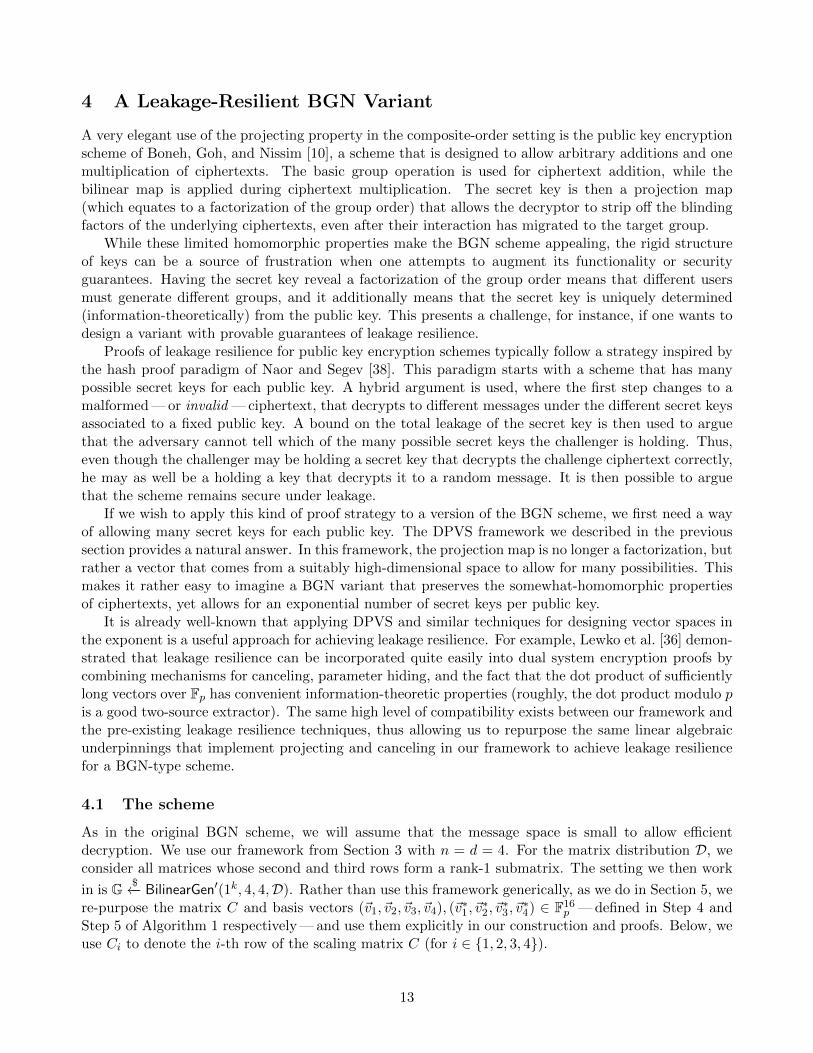
4 A Leakage-Resilient BGN Variant
A very elegant use of the projecting property in the composite-order setting is the public key encryptionscheme of Boneh, Goh, and Nissim [10], a scheme that is designed to allow arbitrary additions and onemultiplication of ciphertexts. The basic group operation is used for ciphertext addition, while thebilinear map is applied during ciphertext multiplication. The secret key is then a projection map(which equates to a factorization of the group order) that allows the decryptor to strip off the blindingfactors of the underlying ciphertexts, even after their interaction has migrated to the target group.
While these limited homomorphic properties make the BGN scheme appealing, the rigid structureof keys can be a source of frustration when one attempts to augment its functionality or securityguarantees. Having the secret key reveal a factorization of the group order means that different usersmust generate different groups, and it additionally means that the secret key is uniquely determined(information-theoretically) from the public key. This presents a challenge, for instance, if one wants todesign a variant with provable guarantees of leakage resilience.
Proofs of leakage resilience for public key encryption schemes typically follow a strategy inspired bythe hash proof paradigm of Naor and Segev [38]. This paradigm starts with a scheme that has manypossible secret keys for each public key. A hybrid argument is used, where the first step changes to amalformed — or invalid — ciphertext, that decrypts to different messages under the different secret keysassociated to a fixed public key. A bound on the total leakage of the secret key is then used to arguethat the adversary cannot tell which of the many possible secret keys the challenger is holding. Thus,even though the challenger may be holding a secret key that decrypts the challenge ciphertext correctly,he may as well be a holding a key that decrypts it to a random message. It is then possible to arguethat the scheme remains secure under leakage.
If we wish to apply this kind of proof strategy to a version of the BGN scheme, we first need a wayof allowing many secret keys for each public key. The DPVS framework we described in the previoussection provides a natural answer. In this framework, the projection map is no longer a factorization, butrather a vector that comes from a suitably high-dimensional space to allow for many possibilities. Thismakes it rather easy to imagine a BGN variant that preserves the somewhat-homomorphic propertiesof ciphertexts, yet allows for an exponential number of secret keys per public key.
It is already well-known that applying DPVS and similar techniques for designing vector spaces inthe exponent is a useful approach for achieving leakage resilience. For example, Lewko et al. [36] demon-strated that leakage resilience can be incorporated quite easily into dual system encryption proofs bycombining mechanisms for canceling, parameter hiding, and the fact that the dot product of sufficientlylong vectors over Fp has convenient information-theoretic properties (roughly, the dot product modulo pis a good two-source extractor). The same high level of compatibility exists between our framework andthe pre-existing leakage resilience techniques, thus allowing us to repurpose the same linear algebraicunderpinnings that implement projecting and canceling in our framework to achieve leakage resiliencefor a BGN-type scheme.
4.1 The scheme
As in the original BGN scheme, we will assume that the message space is small to allow efficientdecryption. We use our framework from Section 3 with n = d = 4. For the matrix distribution D, weconsider all matrices whose second and third rows form a rank-1 submatrix. The setting we then work
in is G $←− BilinearGen′(1k, 4, 4,D). Rather than use this framework generically, as we do in Section 5, were-purpose the matrix C and basis vectors (~v1, ~v2, ~v3, ~v4), (~v
∗1, ~v∗2, ~v∗3, ~v∗4) ∈ F16
p — defined in Step 4 andStep 5 of Algorithm 1 respectively — and use them explicitly in our construction and proofs. Below, weuse Ci to denote the i-th row of the scaling matrix C (for i ∈ {1, 2, 3, 4}).
13

• Setup(G): Pick r, r∗$←− Fp and define ~u :=
∑i ~vi, ~u
∗ :=∑i ~v∗i , ~w := r~v2, and ~w∗ := r∗~v∗2. Choose ~y
uniformly at random from the set of vectors in F4p such that ~y ·C2 = 0, noting that ~y ·C3 = 0 then
holds automatically as well. Output pk = (g, g~u, g ~w, h~u∗, h~w
∗) and sk =
(~y, skT = e(g, h)~y·(
∑iCi)).
Note that, by construction, ~y · (∑iCi) = ~y · (C1 + C4) and, by Lemma 3.5, E(g~u, h~u
∗) =(
e(g, h)∑
jcj,1 , . . . , e(g, h)
∑jcj,4)
.
• Enc(pk ,m): We have two types of ciphertexts: Type A and Type B. If we want to be able toperform homomorphic operations on any pair of ciphertexts, a single ciphertext could include
both types. To form a Type A ciphertext, choose s$←− Fp and compute ctA := gm~u+s~w. To form a
Type B ciphertext, choose s∗$←− Fp and compute ctB := hm~u
∗+s∗ ~w∗ . Output ct = (ctA, ctB). (Orjust ctA or ctB, depending on the desired homomorphic properties.)
• Eval(pk , ct1, ct2): We describe two evaluation cases: addition of Type A ciphertexts (the operationsare analogous for Type B ciphertexts), and multiplication of a Type A and Type B ciphertext(which can then be further added in the target space BT ).
First pick a random value t$←− Fp. If ct1 and ct2 are Type A, then return ct = ct1 · ct2 · gt ~w. If ct1
is Type A and ct2 is Type B, then return ct = E(ct1, ct2) · E(g ~w, h~w∗)t.
• Dec(sk , ct): To decrypt a ciphertext (ct1, ct2, ct3, ct4) ∈ G4T , compute
4∏i=1
ctyii = skmT .
Using knowledge of skT , exhaustively search for m (this is possible since we have a small messagespace). If ct is Type A, then compute ct′ = E(ct,Enc(pk , 1)) and decrypt ct′ (and analogously fora Type B ciphertext).
To see that decryption is correct, observe that∏i
ctyii =∏i
e(g, h)myi
∑jcj,i = e(g, h)
m∑
i
∑jyicj,i
= e(g, h)m∑
j
∑iyicj,i = e(g, h)
m∑
j~y·Cj
= skmT .
To see that evaluation is correct, observe that if ct1 encrypts m1 and ct2 encrypts m2 then
ct = gm1~u+s1 ~w · gm2~u+s2 ~w · gt ~w = g(m1+m2)~u+(s1+s2+t)~w,
which is a properly distributed Type A encryption of m1 +m2. Pairing a Type A ct1 and a Type B ct2similarly yields a properly distributed encryption of m1m2 in the target space, just as in BGN.
4.2 Security analysis
The security model we use is leakage against non-adaptive memory attacks, as defined by Akavia etal. [3, Definition 3]. Briefly, the attacker first declares a leakage function f mapping secret keys to{0, 1}` for a suitably small `. The attacker then receives pk and f(sk), and proceeds as in a standardIND-CPA game; i.e., it outputs two messages m0 and m1, receives an encryption of mb, and wins ifit correctly guesses b. As in the case of the original BGN scheme, it suffices to argue security forchallenge ciphertexts generated in G/H, as security for the ciphertexts generated via the multiplicativehomomorphism follows from the security of ciphertexts in the base groups. While there are severalother interesting models for leakage-resilient PKE security, we choose to work with this one, as it isclean and simple and thus allows us to give a concise demonstration of the use of our framework.
14

Theorem 4.1. If SXDH holds in G and ` ≤ log(p− 1)− 2k, the above construction is leakage resilientwith respect to non-adaptive memory attacks.
As in the typical hash proof system paradigm, we first define invalid ciphertexts that have moreblinding randomness than honestly generated ciphertexts. Initially, these are still decrypted consistentlyby the set of secret keys corresponding to a fixed public key. After having transitioned to a game withan invalid challenge ciphertext, however, we gradually adjust the respective distributions of secret keysand ciphertexts to arrive at a game where, in the adversary’s view, it seems that the secret key decryptsthe ciphertext randomly.
In the course of these game transitions, we use SXDH in multiple ways. First we use it to changefrom an honest to an invalid ciphertext by bringing in an additional blinding factor in a new subgroup.This is just a “nice” instance of subgroup decision. We will also use it to make changes to the rank ofparticular submatrices inside the scaling matrix C. This technique is inspired by the observation in [11]that DDH implies a rank-1 matrix in the exponent is hard to distinguish from a rank-2 matrix. Tomake the crucial switch from a secret key that properly decrypts the challenge ciphertext to a key thatdecrypts it incorrectly, we rely on an information-theoretic argument leveraging a form of parameterhiding, along with the leakage bound. Essentially, the simulator uses the remaining ambiguity in theunderlying parameters (conditioned on the public key) to help it create an invalid challenge ciphertextafter supplying the leakage.
We begin by defining the invalid encryption algorithm that blinds a gm~u payload with a random
term g~δ, where ~δ is sampled uniformly from the span of ~v2, ~v3, instead of just the 1-dimensional span
of ~v2 within this. Similarly, it blinds a hm~u∗
payload with a random term h~δ∗ where ~δ∗ is sampled
uniformly from the span of ~v∗2, ~v∗3 instead of the 1-dimensional span of ~v∗2.
We let Game0 denote the real security game, and Game1 denote a game where the invalid encryptionalgorithm is used to create the challenge ciphertext. Note that the secret key still properly decrypts aninvalid challenge ciphertext. We argue that the attacker’s advantage can change only negligibly as wetransition from Game0 to Game1:
Lemma 4.2. Under the SXDH assumption, no PPT adversary can obtain a non-negligible change inadvantage between Game0 and Game1.
Proof. We show how to accomplish this transition for Type A ciphertexts, relying on the DDH assump-tion in G. This is essentially an instance of Lemma 3.8, but we include the proof here for completeness.The case for Type B ciphertexts is analogous, relying on the DDH assumption in H. If one wants toproduce a joint ciphertext that includes both a Type A and Type B encryption, then one can simplythink of these two separate arguments as forming a hybrid argument for this transition that first changesthe Type A part of the ciphertext and then the Type B part.
Suppose there exists a PPT adversary A whose advantage changes non-negligibly between Game0to Game1 (with a Type A challenge ciphertext). We create a PPT algorithm B that achieves a non-negligible advantage against SXDH. B is given group elements g, ga, gb, T in G, and it is B’s task todetermine if T = gab or is random.
B first samples dual orthonormal bases (F1,F∗1), . . . , (F4,F∗4)$←− Dual(F4
p). It then samples matrix
rows C1, C3, C4$←− F4
p, and a random row C2 from the span of C3. It implicitly sets C2 = aC2. We notethat the resulting C is properly distributed for Game0 and Game1.
B implicitly sets:
~v1 = c11 ~f11||c12 ~f12||c13 ~f13||c14 ~f14, ~v∗1 = ~f∗11||~f∗12||~f∗13||~f∗14,
~v2 = c21(~f21 + a~f31)||c22(~f22 + a~f32)||c23(~f23 + a~f33)||c24(~f24 + a~f34), ~v∗2 = a~f∗21||a~f∗22||a~f∗23||a~f∗24,
15

~v3 = c31 ~f31||c32 ~f32||c33 ~f33||c34 ~f34, ~v∗3 = ~f∗31 − a~f∗21||~f∗32 − a~f∗22||~f∗33 − a~f∗23||~f∗34 − a~f∗24,
~v4 = c41 ~f41||c42 ~f42||c43 ~f43||c44 ~f44, ~v∗4 = ~f∗41||~f∗42||~f∗43||~f∗44.
We note that B can compute g~v1 , g~v2 , g~v3 , and g~v4 , and hence can compute g~u. It can also choose a
random scalar r$←− Fp and compute g ~w := gr~v2 . We observe that ~u∗ = ~f∗1 1+ ~f∗31+ ~f∗41|| . . . ||~f∗14+ ~f∗34+ ~f∗44
is known to B, so it can also compute h~u∗. It chooses a random r
$←− Fp and sets h~w∗
= hr(~f∗21||...||~f
∗24).
Observe that this results in properly distributed public parameters, which it gives to A.Since it knows the span of C2, C3 as well as C1 + C4 it can also honestly sample the secret key
and respond to A’s leakage query. B also has the ability to produce either valid or invalid TypeB ciphertexts (even though it cannot produce h~v
∗3 by itself, it can sample random combinations of
~v∗2, ~v∗3 in the exponent, which are identically distributed to random combinations of (~f∗21|| . . . ||~f∗24) and
(~f∗31|| . . . ||~f∗34)).To create the challenge ciphertext of Type A, B computes:
gmb~uT (c21f31||...||c24f34)(gb)c21~f21||...||c24 ~f24 .
If T = gab, this is equal to gm~u+b~v2 , which is a Type A ciphertext that is properly distributed for Game0.
If T is random, this is distributed as gmb~u+~δ where ~δ is a random linear combination of ~v2 and ~v3. Tosee this, recall that C3 is the span of C2. Hence, if T = gab, B has properly simulated Game0, and if T israndom, then B has properly simulated Game1 (with a Type A challenge ciphertext). So B can leverageA’s difference in advantage between these games to achieve a non-negligible advantage in solving DDHin G.
We now define Game2. In this game, the scaling matrix C is chosen to be a uniformly random 4× 4matrix over Fp (note that it has full rank with high probability). The ciphertext is still produced asan invalid encryption, and the secret key ~y is sampled so that ~y · C2 = 0 = ~y · C3. (There is now a2-dimensional space of such ~y.)
To transition between Game1 and Game2, we use the fact that DDH in G implies the hardness ofdistinguishing a random rank one from a random rank two matrix in the exponent. This was previouslyobserved in [11].
Lemma 4.3. Under DDH in G, no PPT adversary can attain a non-negligible difference in advantagebetween Game1 and Game2.
Proof. We suppose there is a PPT adversary A that exhibits a non-negligible difference in advantagebetween Game1 and Game2, and create a PPT algorithm B that breaks DDH in G with a non-negligibleadvantage. B receives g, ga, gb, h, T = gt. Its task is to guess if t = ab or is random.
B chooses a random 2×4 matrix M over Fp (note with high probability this has rank 2). It implicitlysets C2, C3 equal to the rows of:(
1 ab t
)(m11 m12 m13 m14
m21 m22 m23 m24
)=
(m11 + am21 m12 + am22 m13 + am23 m14 + am24
bm11 + tm21 bm12 + tm22 bm13 + tm23 bm14 + am24
).
B can form gc2i , gc3i for each i using its knowledge of M and g, ga, gb, gt. If t = ab, this is distributedas a random rank-1 matrix. If t is random, this is distributed as a random rank-2 matrix. We furthernote that B can sample a vector ~γ uniformly from the orthogonal space of the rows of M , which remainorthogonal to the implicitly determined rows C2, C3. We claim that ~γ is distributed as a random vectororthogonal to C2, C3 for either case of t. In the case that t is random, this is clear because the spanof C2, C3 is equal to the span of the rows of M . In the case that t = ab, note that M2, the second
16
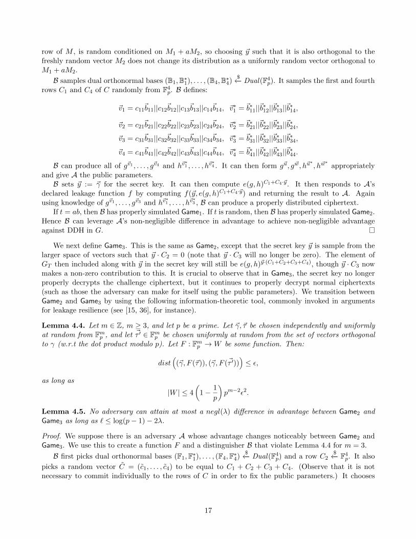
row of M , is random conditioned on M1 + aM2, so choosing ~y such that it is also orthogonal to thefreshly random vector M2 does not change its distribution as a uniformly random vector orthogonal toM1 + aM2.
B samples dual orthonormal bases (B1,B∗1), . . . , (B4,B∗4)$←− Dual(F4
p). It samples the first and fourthrows C1 and C4 of C randomly from F4
p. B defines:
~v1 = c11~b11||c12~b12||c13~b13||c14~b14, ~v∗1 = ~b∗11||~b∗12||~b∗13||~b∗14,
~v2 = c21~b21||c22~b22||c23~b23||c24~b24, ~v∗2 = ~b∗21||~b∗22||~b∗23||~b∗24,
~v3 = c31~b31||c32~b32||c33~b33||c34~b34, ~v∗3 = ~b∗31||~b∗32||~b∗33||~b∗34,
~v4 = c41~b41||c42~b42||c43~b43||c44~b44, ~v∗4 = ~b∗41||~b∗42||~b∗43||~b∗44.
B can produce all of g~v1 , . . . , g~v4 and h~v∗1 , . . . , h~v
∗4 . It can then form g~u, g ~w, h~u
∗, h~w
∗appropriately
and give A the public parameters.B sets ~y := ~γ for the secret key. It can then compute e(g, h)C1+C4·~y. It then responds to A’s
declared leakage function f by computing f(~y, e(g, h)C1+C4·~y) and returning the result to A. Againusing knowledge of g~v1 , . . . , g~v3 and h~v
∗1 , . . . , h~v
∗3 , B can produce a properly distributed ciphertext.
If t = ab, then B has properly simulated Game1. If t is random, then B has properly simulated Game2.Hence B can leverage A’s non-negligible difference in advantage to achieve non-negligible advantageagainst DDH in G.
We next define Game3. This is the same as Game2, except that the secret key ~y is sample from thelarger space of vectors such that ~y · C2 = 0 (note that ~y · C3 will no longer be zero). The element ofGT then included along with ~y in the secret key will still be e(g, h)~y·(C1+C2+C3+C4), though ~y · C3 nowmakes a non-zero contribution to this. It is crucial to observe that in Game3, the secret key no longerproperly decrypts the challenge ciphertext, but it continues to properly decrypt normal ciphertexts(such as those the adversary can make for itself using the public parameters). We transition betweenGame2 and Game3 by using the following information-theoretic tool, commonly invoked in argumentsfor leakage resilience (see [15, 36], for instance).
Lemma 4.4. Let m ∈ Z, m ≥ 3, and let p be a prime. Let ~γ, ~τ be chosen independently and uniformlyat random from Fmp , and let ~τ ′ ∈ Fmp be chosen uniformly at random from the set of vectors orthogonalto γ (w.r.t the dot product modulo p). Let F : Fmp →W be some function. Then:
dist((~γ, F (~τ)), (~γ, F (~τ ′))
)≤ ε,
as long as
|W | ≤ 4
(1− 1
p
)pm−2ε2.
Lemma 4.5. No adversary can attain at most a negl(λ) difference in advantage between Game2 andGame3 as long as ` ≤ log(p− 1)− 2λ.
Proof. We suppose there is an adversary A whose advantage changes noticeably between Game2 andGame3. We use this to create a function F and a distinguisher B that violate Lemma 4.4 for m = 3.
B first picks dual orthonormal bases (F1,F∗1), . . . , (F4,F∗4)$←− Dual(F4
p) and a row C2$←− F4
p. It also
picks a random vector C = (c1, . . . , c4) to be equal to C1 + C2 + C3 + C4. (Observe that it is notnecessary to commit individually to the rows of C in order to fix the public parameters.) It chooses
17

random values αij , α∗ij ∈ Fp for i, j ∈ [4] up to the constraints that α2j = 1 and α∗2j = c2j for each j,
and∑i αijα
∗ij = cj for each j. It sets:
~v2 := ~f21||~f22||~f23||~f24,
~v∗2 := c21 ~f∗21||c22 ~f∗22||c23 ~f∗23||c24 ~f∗24,
~u := α11~f11 + α21
~f21 + · · ·+ α41~f41|| . . . ||α14
~f14 + · · ·+ α44~f44,
~u∗ := α∗11~f∗11 + α∗21
~f∗21 + · · ·+ α∗41~f∗41|| . . . ||α∗14 ~f∗14 + · · ·+ α∗44
~f∗44.
This allows it to produce public parameters, which it gives to A.Next, A declares a leakage function f to be applied to ~y and e(g, h)C·~y. B fixes a 4 × 3 matrix M
over Fp such that M is a bijection from 3-dimensional vectors over Fp into the orthogonal space of C2
inside F4p and also that MTM is equal to the 3 × 3 identity matrix over Fp. It implicitly sets ~y = M~τ
and defines F such that F (~τ) = f(~y, e(g, h)C·~y). It then receives ~γ, F (~τ) and forwards F (~τ) to A as theresponse to the leakage query.
B now chooses a random scalar t$←− Fp and sets C3 = M~γ+ tC2. Note that with high probability, C2
is not self-orthogonal, and hence not in the image of M , and this will then be properly distributed as arandom vector. The task for B is now to find settings for ~v1, ~v3, ~v4, ~v
∗1, ~v∗3, ~v∗4 that are consistent with the
values of C, C3, ~u, ~u∗, ~v2, ~v
∗2. This is an instance of parameter-hiding: essentially B will take advantage
of the fact that the values it previously committed to did not in fact determine C3. We show how it isable to leverage the remaining degrees of freedom in the parameter settings to now accommodate thisfreshly chosen value of C3.
We consider the first four coordinates of the ~vi and ~v∗i first (and then we consider the next block offour coordinates, etc.). Our goal is to define suitable values of c11, c41 and suitable matrices A,A∗ ofthe form
A :=
a11 0 a13 a140 1 0 0a31 0 a33 a34a41 0 a43 a44
, A∗ :=
a∗11 0 a∗13 a∗140 c21 0 0a∗31 0 a∗33 a∗34a∗41 0 a∗43 a∗44
such that
~v1 = a11 ~f11 + a13 ~f31 + a14 ~f41, ~v∗1 = c11(a∗11~f∗11 + a∗13
~f∗31 + a∗14~f∗41),
~v3 = a31 ~f11 + a33 ~f31 + a34 ~f41, ~v∗3 = c31(a∗31~f∗11 + a∗33
~f∗31 + a∗34~f∗41),
~v4 = a41 ~f11 + a43 ~f31 + a44 ~f41, ~v∗4 = c41(a∗41~f∗11 + a∗43
~f∗31 + a∗44~f∗44)
is a valid setting. For this, we need A∗ = (A−1)T , and we need
α11 = a11 + a31 + a41, α∗11 = c11a∗11 + c31a
∗31 + c41a
∗41,
α31 = a13 + a33 + a43, α∗31 = c11a∗13 + c31a
∗33 + c41a
∗43,
α41 = a14 + a34 + a44, α∗41 = c11a∗14 + c31a
∗34 + c41a
∗44.
To see how to solve this system of equations, we first define the matrix
B =
1 0 00 0 01 1 1
.
18

We then observe that a matrix A will satisfy the linear restrictions above imposed by α11, α31, α41
whenever A is of the form
A = B−1 ·
r t us v wα11 α31 α41
,where r, t, u, s, v, w are free variables. We can then express the other constraints as:
(c11 c31 c41)(A−1)T = (α∗11 α
∗31 α
∗41),
which we may rewrite as
(c11 c31 c41)B = (α∗11 α∗31 α
∗41)
r s α11
t v α31
u w α41
.It is easy to see that by choosing r, t, u, s, v, w appropriately, we can make the right-hand side of thisexpression equal to any vector in F3
p whose final coordinate is α11α∗11 + α31α
∗31 + α41α
∗41. Thus, for any
choice of c11 and c41 such that c11 + c31 + c41 equal this value, we can solve for r, s, t, u, v, w, and hencefor the first four coordinates of the vectors ~v1, ~v3, ~v4, ~v
∗1, ~v∗3, ~v∗4.
B can similarly solve for suitable values for the remaining 12 coordinates of these vectors by consid-ering each 4-coordinate block in a similar fashion. Note that applying different matrices A and (A−1)T
as a change of basis for each (Fi,F∗i ) still results in a proper distribution of random dual orthonormalbases in each block of 4 coordinates. Once B has determined properly distributed values of ~v1, ~v3, ~v4,~v∗1, ~v∗3, ~v∗4, it can easily form a properly distributed challenge ciphertext.
We observe that when ~τ , ~δ are orthogonal, ~y and C3 are also orthogonal (and ~y is distributedrandomly up to the constraint that it is orthogonal to C2 and C3). In this case, B properly simulatesGame2. However, when ~τ , ~δ are uniformly random, then ~y is distributed randomly up to the constraintthat it is orthogonal to C2, and hence B properly simulates Game3. Lemma 4.4 thus implies Lemma 4.5.
We next define Game4, which is the same as Game3 except that C is sampled so that C1, C2 arerandom, and C3, C4 are sampled randomly from the span of C1.
Lemma 4.6. Under DDH in G, no PPT adversary can attain a non-negligible difference in advantagebetween Game3 and Game4.
Proof. We accomplish this transition in two phases, first moving to a Game3.5 where C1, C2, C4 arerandom, and C3 is sampled from the span of C1. We start by supposing there is a PPT adversary Athat exhibits a non-negligible difference in advantage between Game3 and Game3.5, and create a PPTalgorithm B that breaks DDH in G with a non-negligible advantage. B receives g, ga, gb, h, T = gt. Itstask is to guess if t = ab or random.
As in the proof of Lemma 4.3, B chooses a random matrix M and implicitly sets C1, C3 equal to therows of (
1 ab t
)(m11 m12 m13 m14
m21 m22 m23 m24
).
B samples dual orthonormal bases (B1,B∗1), . . . , (B4,B∗4)$←− Dual(F4
p). It samples C2, C4$←− F4
p.B defines:
~v1 = c11~b11||c12~b12||c13~b13||c14~b14, ~v∗1 = ~b∗11||~b∗12||~b∗13||~b∗14,
~v2 = c21~b21||c22~b22||c23~b23||c24~b24, ~v∗2 = ~b∗21||~b∗22||~b∗23||~b∗24,
19
~v3 = c31~b31||c32~b32||c33~b33||c34~b34, ~v∗3 = ~b∗31||~b∗32||~b∗33||~b∗34,
~v4 = c41~b41||c42~b42||c43~b43||c44~b44, ~v∗4 = ~b∗41||~b∗42||~b∗43||~b∗44.
B can produce all of g~v1 , . . . , g~v4 and h~v∗1 , . . . , h~v
∗4 using g, h, ga, gb, gt. It can then produce g~u, g ~w, h~u
∗, h~w
∗
appropriately and give A the public parameters.To form the secret key, B samples a random vector ~y such that ~y · C2 = 0. We note that it can
compute e(g, h)(C1+C3+C4)·~y because it can compute each e(g, h)c1i and e(g, h)c3i and it knows ~y. Thisallows B to respond to the leakage query made by A.
Using knowledge of g~v1 , . . . , g~v3 and h~v∗1 , . . . , h~v
∗3 , B can produce a properly distributed ciphertext.
Now, if t = ab, B has properly simulated Game3. If t is random, B has properly simulated Game3.5.Hence it can leverage A’ difference in advantage to break DDH. We can similarly rule out a PPTadversary that distinguishes between Game3.5 and Game4.
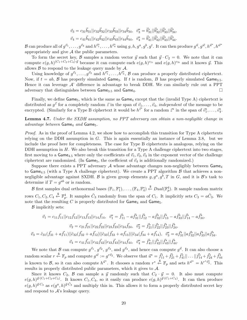
Finally, we define Game5, which is the same as Game4 except that the (invalid Type A) ciphertext isdistributed as g~z for a completely random ~z in the span of ~v1, . . . , ~v4, independent of the message to beencrypted. (Similarly for a Type B ciphertext it would be h~z
∗for a random ~z∗ in the span of ~v∗1, . . . , ~v
∗4.
Lemma 4.7. Under the SXDH assumption, no PPT adversary can obtain a non-negligible change inadvantage between Game4 and Game5.
Proof. As in the proof of Lemma 4.2, we show how to accomplish this transition for Type A ciphertextsrelying on the DDH assumption in G. This is again essentially an instance of Lemma 3.8, but weinclude the proof here for completeness. The case for Type B ciphertexts is analogous, relying on theDDH assumption in H. We also break this transition for a Type A challenge ciphertext into two stages,first moving to a Game4.5 where only the coefficients of ~v1, ~v2, ~v3 in the exponent vector of the challengeciphertext are randomized. (In Game5, the coefficient of ~v4 is additionally randomized.)
Suppose there exists a PPT adversary A whose advantage changes non-negligibly between Game4to Game4.5 (with a Type A challenge ciphertext). We create a PPT algorithm B that achieves a non-negligible advantage against SXDH. B is given group elements g, ga, gb, T in G, and it is B’s task todetermine if T = gab or is random.
B first samples dual orthonormal bases (F1,F∗1), . . . , (F4,F∗4)$←− Dual(F4
p). It sample random matrix
rows C1, C2, C4$←− F4
p. It samples C3 randomly from the span of C1. It implicitly sets C3 = aC3. Wenote that the resulting C is properly distributed for Game4 and Game5.
B implicitly sets:
~v1 = c11 ~f11||c12 ~f12||c13 ~f13||c14 ~f14, ~v∗1 = ~f∗11 − a~f∗31||~f∗12 − a~f∗32||~f∗13 − a~f∗33||~f∗14 − a~f∗34,
~v2 = c21 ~f21||c22 ~f22||c23 ~f23||c24 ~f24, ~v∗2 = ~f∗21||~f∗22||~f∗23||~f∗24,
~v3 = c31(~f31 + a~f11)||c32(~f32 + a~f12)||c33(~f33 + a~f13)||c34(~f34 + a~f14), ~v∗3 = a~f∗31||a~f∗32||a~f∗33||a~f∗34,
~v4 = c41 ~f41||c42 ~f42||c43 ~f43||c44 ~f44, ~v∗4 = ~f∗41||~f∗42||~f∗43||~f∗44.
We note that B can compute g~v1 , g~v2 , g~v3 , and g~v4 , and hence can compute g~u. It can also choose a
random scalar r$←− Fp and compute g ~w := gr~v2 . We observe that ~u∗ = ~f∗11+ ~f∗21+ ~f∗41|| . . . ||~f∗14+ ~f∗24+ ~f∗44
is known to B, so it can also compute h~u∗. It chooses a random r∗
$←− Fp and sets h~w∗
= hr∗~v∗2 . This
results in properly distributed public parameters, which it gives to A.Since it knows C2, B can sample a ~y randomly such that C2 · ~y = 0. It also must compute
e(g, h)~y·(C1+C3+C4). It knows C1, C4, so it easily can produce e(g, h)~y·(C1+C4). It can then produce
e(g, h)~y·C3 as e(ga, h)~y·C3 and multiply this in. This allows it to form a properly distributed secret keyand respond to A’s leakage query.
20
We note that B also has the ability to produce invalid Type B ciphertexts, as it can sample randomcombinations of ~v∗2, ~v
∗3 in the exponent, which are identically distributed to random combinations of
(~f∗21|| . . . ||~f∗24) and (~f∗31|| . . . ||~f∗34)). Furthermore, it can produce Type B ciphertexts as they wouldbe distributed in Game5, as random linear combinations of ~v∗1, . . . , ~v
∗4 are identically distributed to
random linear combinations of (~f∗11|| . . . ||~f∗14), . . . , (~f∗41|| . . . ||~f∗44). (This would be needed to do a hybridargument for a joint ciphertext that has both Type A and Type B parts.)
To create the challenge ciphertext of Type A, B chooses a random t$←− Fp and computes:
gmb~ugt~v2T (c31f11||...||c34f14)(gb)c31~f31||...||c34 ~f34 .
If T = gab, this is equal to gm~u+t~v2+b~v3 , which is a Type A ciphertext that is properly distributed for
Game4. If T is random, this is distributed as gmb~u+~δ where ~δ is a random linear combination of ~v1, ~v2,and ~v3. To see this, recall that C1 is the span of C3. Hence, if T = gab, B has properly simulated Game4,and if T is random, then B has properly simulated Game4.5 (with a Type A challenge ciphertext). So Bcan leverage A’s difference in advantage between these games to achieve a non-negligible advantage insolving DDH in G.
The transition from Game4.5 to Game5 with a Type A ciphertext is analogous, just with the roles ofC1 and C4 reversed (note that both are in the span of C3).
This completes the proof of leakage resilience for our scheme.
5 An IBE with IND-CCA1 Security
The second application we provide is an IND-CCA1-secure identity-based encryption scheme. AlthoughIND-CCA2-secure IBE schemes have already been constructed, we believe our techniques are moregenerally useful beyond this single application.
At its heart, our construction can be thought of as a variant on the Boneh-Boyen scheme, whichis IND-CPA secure (and is clearly not IND-CCA2 secure, as it has re-randomizable ciphertexts). Byadding in various components in different subgroups, we first show (using canceling, parameter hiding,and subgroup decision variants) that our construction satisfies a weak notion of IND-CCA1 security,in which the adversary does not even get to see the public parameters. While such a notion mightnot seem to be very useful on its own, we next show that, by folding in weak projecting for additionalsubgroups, we are able to boost up to full IND-CCA1 security. This is a new application of projectingthat requires only a mild expansion of the structure of the original scheme and fits in nicely with theevolution of dual system encryption techniques.
The high-level idea of the construction and proof is as follows. We start with the core Boneh-Boyenconstruction and embed it into groups with several canceling subgroups; we then add decryption checksto confirm that the ciphertext conforms to the appropriate structure in certain subgroups. Now, weobserve that if an adversary is not given the public parameters, it can attempt to produce well-formeddecryption queries only using the information it gains from key requests. We can apply a dual-systemencryption approach to add random components to these keys in a subgroup that we also add to theciphertext. Now, since everything in this “semi-functional” subgroup is randomized, the adversarycannot learn the appropriate structure that is being tested for by the decryption oracle. Hence, theonly successful decryption queries it can produce must avoid this semi-functional space; we can use anadversary who produces such a query while receiving elements with random semi-functional components,however, to break a variant of subgroup decision. In this weak security game where no public parametersare given out, we can therefore prove IND-CCA1 security. Our notion of the weak game here is inspiredby the new interpretation of dual system encryption techniques developed by Lewko and Waters [33].
21

To reduce full IND-CCA1 security to this weak version, we enlarge the space of our weakly securescheme by adding two more subgroups so that we can project separately onto the components of theembedded scheme and the additional space; our construction then places meaningful components onlyin this additional space. To prove security, we first expand into the embedded space using a variant ofsubgroup decision. We now have a “shadow” copy of the scheme, attached to both keys and ciphertexts,that is not reflected in the public parameters, and we can project separately onto the real copy andonto this shadow copy. Thus, we can reduce full security to the weak security of the shadow schemeby having the reduction create the components in the real space itself and use projection to interpolatebetween an adversary on the full game and a challenger for the weak game.
5.1 An IBE with weak IND-CCA1 security
We first define a weak version of IND-CCA1 security for IBE, in which the adversary does not get tosee the full public parameters, but only the bilinear group:
Definition 5.1. For a bilinear group generator BilinearGen, an IBE (Setup,KeyExt,Enc,Dec), an ad-versary A, and a bit b, let pA
b (k) be the probability of the event that b′ = 0 in the following game:
• Step 1. G $←− BilinearGen(1k, n); (params,msk)$←− Setup(G).
• Step 2. (state,m0,m1, id∗)
$←− ADec(params,msk ,·,·),KeyExt(params,msk ,·)(G).
• Step 3. If |m0| 6= |m1| or A queried its KeyExt oracle on id∗, output ⊥. Otherwise, output
ct∗$←− Enc(params, id∗,mb).
• Step 4. b′$←− AKeyExt(params,msk ,·)(state, ct∗).
We say that the IBE satisfies weak IND-CCA1 security if for all PPT algorithms A there exists anegligible function ν(·) such that |pA
0 (k)− pA1 (k)| < ν(k).
For our bilinear group, we require six subgroups on each side of the pairing; this means we run G =
(N,G,H,GT , e, {gi}i, {hi}i, µ)$←− BilinearGen′(1k, 6), where G := ⊕6
i=1Gi = 〈gi〉, H := ⊕6i=1Hi = 〈hi〉,
e : G ×H → GT , µ allows one to check membership in both G and H, and N is the maximum orderof any element in these groups. We require that the message space is the cyclic subgroup generatedby e(g1, h1) in GT . Our construction relies generically on the structure of the group and thus can beinstantiated, as we see below, in either composite-order groups, using N as a product of distinct primes,or prime-order groups, using N as a prime. In addition to the regular canceling (and parameter hiding)requirements, we also require that specific generators gi ∈ Gi and hi ∈ Hi for all i, 1 ≤ i ≤ 4, are chosensuch that
e(g1g2, h1h2) = e(g3g4, h3h4) = 1. (2)
Although this might seem like an additional requirement, as we see below and in Section 6, this propertycan be trivially constructed in prime-order and composite-order settings that satisfy the regular notionof canceling. This same sort of reorganization could also be applied to the original Boneh-Boyenconstruction by conceptualizing keys and ciphertexts as single elements in G×G instead of as pairs ofelements in G, and more generally we consider the distinction between single group elements in a largergroup and tuples of elements in a smaller group a matter of taste. (Of course, thinking of G × G asa single group results in certain cases of subgroup decision problems being easy, such as distinguishingG× 1G from G×G, but these cases will not come up.) Armed with such a bilinear group, we begin bypresenting our IBE construction.
• Setup(G): Parse G = (N,G,H,GT , e, {gi}6i=1, {hi}6i=1, µ) and pick α$←− Z/NZ. Output params :=
((N,G,H,GT , e, µ), g1, g2, A := e(g1, h1)α) and msk := (hα1 , {hi}6i=1).
22

• KeyExt(params,msk , id): Pick t, t′, γ, γ′, β, β′$←− Z/NZ and compute sk id ,1 := hα1h
tid1 ht2h
γ5h
β6 and
sk id ,2 := ht′id1 ht
′2 h
γ′
5 hβ′
6 Output sk id := (sk id ,1, sk id ,2).
• Enc(params, id ,M): Pick s$←− Z/NZ and compute ct1 := M · As and ct2 := gs1 · gsid2 . Output
ct := (ct1, ct2).
• Dec(params, sk id , ct): Check that ct2 ∈ G and that e(ct2, sk id ,2) = 1; output ⊥ if either of thesedoes not pass. Otherwise, output M := ct1 · e(ct2, sk id ,1)
−1.
We note that msk can be used to decrypt directly; i.e., rather than form sk id and decrypt in theusual way, we can instead compute M = ct1 · e(ct2, hα1 )−1.
Lemma 5.2. If canceling and Equation 2 hold in G, then the above construction describes a correctidentity-based encryption scheme.
Proof. To see that, for all identities id and messages M , sk id$←− KeyExt(params,msk , id) correctly
decrypts a ciphertext ct$←− Enc(params, id ,M), we first observe that the decryption check will pass, as
e(ct2, ht′id1 ht
′2 h
γ′
5 hβ′
6 ) = e(gs1 · gsid2 , hid1 h2)t′ = e(gs1, h
id1 )t
′ · e(gsid2 , h2)t′ = (e(g1, h1)e(g2, h2))
st′id = 1,
where the first equality follows from canceling and the last equality follows from Equation 2. Addition-ally, decryption succeeds in recovering the message, as
ct1 · e (ct2, sk id ,1)−1 = M ·As · e(gs1gsid2 , hα1 · htid1 · ht2 · h
γ5 · h
β6 )−1
= M · e(g1, h1)αs · e(gs1, hα1 · htid1 )−1 · e(gsid2 , ht2)−1
= M · e(g1, h1)αs · e(g1, h1)−αs · e(g1, h1)−stid · e(g2, h2)−stid
= M · e(g1, h1)−stide(g2, h2)−stid
= M · (e(g1, h1)e(g2, h2))−stid
= M,
where the second equality again follows from canceling and the last from Equation 2.
Theorem 5.3. If canceling, parameter hiding, Equation 2, and generalized correlated subgroup decisionhold in G, then the above construction describes a weakly IND-CCA1-secure identity-based encryptionscheme.
To actualize these abstract requirements, for completeness we consider in Section 6 how they aresatisfied in a composite-order bilinear group. In the prime-order setting, we already gave our augmentedBasicGen construction in Section 3 (which we recall uses n = 8, d = 1, a scaling matrix C with all 1entries, and auxiliary information µ that allows for a membership test in the first six subgroups),and proved that it satisfied canceling and parameter hiding, and that all nice instances of generalizedcorrelated subgroup decision hold if SXDH holds. Our construction also uses gi = g~vi and hi = h−~v
∗i ,
so the definition of dual orthonormal bases ensures that Equation 2 holds as well. As all the instanceswe use in our proof are nice, we have the following corollary:
Corollary 5.4. If SXDH holds in G $←− BasicGen(1k) and G uses augmented information µ, whereBasicGen and augmented µ are as specified in Section 3 , then the instantiation of the above constructionin G is a weakly IND-CCA1-secure identity-based encryption scheme with identity space Fp and messagespace GT .
To prove Theorem 5.3, we proceed through a series of game transitions as follows; formal descriptionsof the games and proofs of their indistinguishability can be found in Appendix A.
23

• Game0. The honest weak IND-CCA1 game.
• Game1. Switch to adding in a “duplicate” component in G3 ⊕G4 to the challenge ciphertext ct∗2;i.e., the value gs
′3 g
s′id4 . This is indistinguishable from Game0 by subgroup decision.
• Game2. Switch the G3⊕G4 component in ct∗2 to be uniformly random. This is identical to Game1by parameter hiding.
• Game3. Switch the keys returned by KeyExt to have random components in H3⊕H4 on sk id ,1 andon sk id ,2; i.e., values hs
′3 h
s′′4 (different values of s′, s′′ for sk id ,1 and sk id ,2). This is indistinguishable
from Game2 using a hybrid argument relying on subgroup decision and parameter hiding.
• Game4. Switch from performing the decryption check with a term of the form ht′id1 ht
′2 h
γ′
5 hβ′
6 to
using a term of the form ht′id1 ht
′2 h
t′′id3 ht
′′4 h
γ′
5 hβ′
6 . This is indistinguishable from Game3 by subgroupdecision.
• Game5. Switch the Dec oracle to return ⊥ on every query in which ct2 6= 1, and 1 if ct2 = 1. Thisis indistinguishable from Game4 by subgroup decision and parameter hiding.
• Game6. Switch to encrypting a random message in the challenge ciphertext. This is indistinguish-able from Game5 by subgroup decision; furthermore, as there is now no information about the bitb, any adversary playing this game has advantage exactly zero.
5.2 Boosting to full IND-CCA1 security
With a weak IND-CCA1-secure IBE in place, we now consider how to augment it to achieve full IND-CCA1 security. Briefly, we do this by adding extra subgroups: to start, we assume we have a bilinear
group G := (N, G, H, GT , e, µ)$←− BilinearGen(1k, 8); i.e., a group such that G := ⊕8
i=1Gi = 〈gi〉,H := ⊕8
i=1Hi = 〈hi〉, and e : G × H → GT , and µ allows one to efficiently test membership in G andH. Once again, these subgroups should all be canceling, and satisfy
e(g1g2, h1h2) = e(g3g4, h3h4) = e(g7g8, h7h8) = 1. (3)
for a particular choice of generators gi, hi. Additionally, the group generation process should alsoproduce a trapdoor τ that allows for the efficient computation of projection maps πG and πH such thatπG : G→ G1 ⊕ . . .⊕ G6 and πH : H → H1 ⊕ . . .⊕ H6; i.e., these map into subgroups analogous to theones that we used in our construction of a weak IND-CCA1-secure IBE.
Finally, if we consider explicitly the group G = (N,⊕6i=1Gi,⊕6
i=1Hi, GT , e, µ) from our weakly secureconstruction, then it should be the case that from G one can create G := (N, G, H, GT , e, µ) such thatGi = Gi and Hi = Hi for all i, 1 ≤ i ≤ 6, and τ can be derived from knowledge of µ. The message spaceand the space of possible identities are the same for the full scheme and the embedded weak scheme.
In our reduction to the weak IND-CCA1 security, we crucially rely on these projection maps, aswell as one other property: if the groups G and H are generated from scratch, then generators forevery subgroup will be known. If the groups are instead generated from the group description for theweak scheme, however, then not all such generators are known; we require that knowledge of suitablegenerators g7, g8, h7, and h8 be incorporated in τ , but the rest of the generators may be unknown.
We now give our construction in this framework:
• Setup(G): Parse G = (N, G, H, GT , e, µ, {gi}8i=1, {hi}8i=1) and pick α$←− Z/NZ. Output params :=
(N, G, H, GT , e, µ), g7, g8, A := e(g7, h7)α) and msk := (hα7 , {hi}8i=1).
• KeyExt(params,msk , id): Pick t, t′, γ, γ′, δ, δ′$←− Z/NZ and compute sk id ,1 := hα7 · htid7 · ht8 · h
γ5 · hδ6
and sk id ,2 := ht′id7 · ht′8 · h
γ′
5 · hδ′
6 . Output sk id := (sk id ,1, sk id ,2).
• Enc(params, id ,M): Pick s$←− Z/NZ and compute ct1 := M · As, ct2 := gs7 · gsid8 . Output
ct := (ct1, ct2).
24

• Dec(params, sk id , ct): First check that ct2 ∈ G and that e(ct2, sk id ,2) = 1; output ⊥ if equalitydoes not hold. Otherwise, output M := ct1 · e(ct2, sk id ,1)
−1.
We note that decryption can again be simplified using msk ; in this case, we compute M = ct1 ·e(ct2, h
α7 )−1.
Lemma 5.5. If canceling and Equation 3 hold in G, then the above construction describes a correctidentity-based encryption scheme.
Proof. To see that, for all identities id and messages M , sk id$←− KeyExt(params,msk , id) correctly
decrypts ct$←− Enc(params, id ,M), we first observe that the decryption check will pass, as e(ct2, h
γ′
5 hδ′6 ) =
1 by canceling, and
e(ct2, ht′id7 ht
′8 ) = e(gs7 · gsid8 , ht
′id7 ht
′8 ) = (e(g7, h7)e(g8, h8))
st′id = 1.
by canceling and Equation 3.To additionally see that decryption will succeed in recovering the message, we have
ct1 · e(ct2, sk id ,1)−1 = M ·As · (e(gs7 · gsid8 , hα7 · htid7 · ht8 · h
γ5 · h
β6 )−1
= M · e(g7, h7)αs · e(gs7, hα7 · htid7 )−1 · e(gsid8 , ht8)−1
= M · e(g7, h7)αs · e(g7, h7)−αs · e(g7, h7)−stid · e(g8, h8)−stid
= M · (e(g7, h7)e(g8, h8))−stid
= M,
where the second equality again follows from canceling and the last from Equation 3.
Theorem 5.6. If weak projecting, canceling, parameter hiding, Equation 3, and generalized correlatedsubgroup decision hold in G, then the above construction is a IND-CCA1-secure identity-based encryptionscheme.
As we did for our weak IBE construction, we consider how to actualize these abstract requirements inboth the composite-order and prime-order settings; for completeness, our composite-order constructionand proofs that it satisfies these requirements can be found in Section 6. For the prime-order setting, wecan now use our BasicGen construction from Section 3; here, as G = G8, we can use our non-augmentedconstruction, as testing membership in G reduces to testing membership in G. We have already provedthis setting satisfies weak projecting, canceling, and parameter hiding, and that the nice instances ofgeneralized correlated subgroup decision hold if SXDH holds. As with our weak IBE, Equation 3 holdstrivially by the definition of dual orthonormal bases.
We must also consider how to embed G into G as described above; this is also quite simple, however,as we can simply use Gi = Gi. The augmented auxiliary information µ for the weak scheme furthermoreenables computation of the projection maps πG and πH , as knowledge of the spans of {~v1, . . . , ~v6} and{~v∗1, . . . , ~v∗6} allows one to compute a linear transformation that projects from F8
p onto these spans, whichcan then be applied in the exponent to map onto G1 ⊕ . . .⊕G6 and H1 ⊕ . . .⊕H6.
As all of the instances of generalized correlated subgroup decision that we use in our proof ofTheorem 5.6 are nice, we obtain the following corollary:
Corollary 5.7. If SXDH holds in G, where G is constructed from G $←− BasicGen(1k) as described above,then the instantiation of the above construction in G is an IND-CCA1-secure identity-based encryptionscheme with identity space Fp and message space GT .
25

To prove Theorem 5.6, we proceed through the following series of game transitions:
• Game0. The honest IND-CCA1 game.
• Game1. Switch the secret keys returned by KeyExt to have additional “duplicate” elements inH1⊕ H2 attached; i.e., elements of the form hβ1 h
t′id1 ht
′2 on sk id ,1 and ht
′′id1 ht
′′2 on sk id ,2. Switch Dec
to use hβ1 hα7 in place of just hα7 , and use a term of the form ht
′′id1 ht
′′2 h
tid7 ht8h
γ′
5 hδ′6 for the decryption
check. This is indistinguishable from Game0 by subgroup decision.
• Game2. Switch the challenge ciphertext to add “duplicate” terms e(g1, h1)βs′ to ct∗1 and gs
′1 g
s′id2
to ct∗2. This is indistinguishable from Game1 by subgroup decision.
Finally, we show that if an adversary can win Game2 then, using weak projection, it can be usedto construct an adversary that breaks the weak IND-CCA1 security of the underlying scheme (i.e., thescheme constructed in the previous section). We therefore reduce the full IND-CCA1 security of thisscheme to the weak IND-CCA1 security of the embedded scheme.
Following this outline, we begin by adding in extra components to secret keys, and changing de-cryption accordingly.
Game0, Game1
1 (N, G, H, GT , e, {gi}8i=1, {hi}8i=1)$←− BilinearGen(1k, 8); G← (N, G, H, GT , e)
2 α$←− Z/NZ, α, β
$←− Z/NZ ; A← e(g7, h7)α, msk ← hα7 , msk ← hβ1 h
α7
3 params ← (G, g1, g2, h1, h2, A)
4 (state,M0,M1, id∗)
$←− AKeyExt,Dec(G)
5 b$←− {0, 1}∗
6 s$←− Z/NZ; ct∗1 ←Mb ·As, ct∗2 ← gs7 · gsid
∗8
7 b′$←− AKeyExt(state, (ct∗1, ct
∗2))
Procedure KeyExt(id)
8 t, t′, γ, γ′, δ, δ′$←− Z/NZ, t, t′, t′′, t′′′, γ, δ, γ′, δ′
$←− Z/NZ9 return sk1
id := hα7 · htid7 · ht8 · hγ5 · hδ6, sk2
id := ht′id7 · ht′8 · h
γ′
5 · hδ′
6
return sk id ,1 := hβ1 ht′′id1 ht
′′2 · hα7 htid7 · ht8 · h
γ5 · hδ6, sk id ,2 := ht
′′′id1 ht
′′′2 ht
′id7 · ht′8 · h
γ′
5 · hδ′
6
Procedure Dec(id , (ct1, ct2))
10 t, γ, δ$←− Z/NZ, t, t′, γ, δ
$←− Z/NZ
11 if e(ct2, htid7 ht8h
γ5h
δ6) 6= 1 return ⊥ if e(ct2, h
t′id1 ht
′2 h
tid7 ht8h
γ5h
δ6) 6= 1 return ⊥
12 return ct1 · e(ct2,msk)−1
Lemma 5.8. If the generalized correlated subgroup decision assumption holds, then Game0 is computa-tionally indistinguishable from Game1.
Proof. We assume there exists an adversary A that can distinguish between Game0 and Game1 withsome non-negligible advantage and use it to construct an adversary B that solves an instance of thegeneralized correlated subgroup decision problem with related non-negligible advantage. We invokethe instance of the assumption parameterized by sets Ssgh
G := {{7, 8}, ∅}, SsghH := {{3, 4, 5, 6, 7, 8}, ∅},
T1 = {(7, 8)}, and T2 = {(1, 2), (7, 8)}, with challenge terms in H.
26

B receives as input G = (N, G, H, GT , e) and elements
(g7, g8, h3, . . . , h8, T, T′),
where either (T, T ′) = (hv7, hv8) or (T, T ′) = (hv7h
z1, h
v8h
z2) for v, z
$←− Z/NZ. B implicitly sets α = v andgives params := (G, g7, g8, e(g7, T )) to A.
On KeyExt queries for an identity id , B picks random t, t′, δ, δ′, σ, σ′, η, η′$←− Z/NZ and returns
sk id ,1 := T · T ηid · (T ′)ηhtid7 ht8hδ5hσ6 , sk id ,2 := T η
′id · (T ′)η′ ht′id7 ht′8 h
δ′5 h
σ′6 ,
Note that if (T, T ′) = (hv7, hv8), this is distributed as in Game0. If instead (T, T ′) = (hv7h
z1, h
v8h
z2), then
this is distributed as in Game1, with β := z.
On Dec queries for (id , (ct1, ct2)), B picks random values t′, δ′, σ′, η′$←− Z/NZ and checks that
e(ct2, Tη′id · (T ′)η′ ht′id7 ht
′8 h
δ′5 h
σ′6 ) = 1 and outputs ⊥ if this check fails. Otherwise, it returns
M := ct1 · e(ct2, T hid7 h8)−1.
Note that if T = hv7, this will produce the same responses as the decryption oracle in Game0, and ifT = hv7h
z1, this will produce the same responses as the decryption oracle in Game1.
Since B knows the public parameters, it can simply use the regular encryption algorithm to producethe challenge ciphertext. It can therefore leverage A’s non-negligible advantage in distinguishing betweenGame0 and Game1 to achieve a non-negligible advantage against this instance of the correlated subgroupdecision problem.
Next, in Game2, we add in duplicate components to the challenge ciphertext as well. This meanschanging Game1 as follows:
Game1, Game2
6 s$←− Z/NZ, s, s′
$←− Z/NZ ; ct∗1 ←Mb ·As, ct∗1 ←Mb ·As · e(g1, h1)βs′
,
ct∗2 ← gs7 · gsid∗
8 , ct∗2 ← gs7 · gsid∗
8 · gs′1 · gs′id∗
2
Lemma 5.9. If the generalized correlated subgroup decision assumption holds, then Game1 is computa-tionally indistinguishable from Game2.
Proof. We assume there exists an adversary A that can distinguish between Game1 and Game2 with somenon-negligible advantage and use it to construct an adversary B that solves an instance of the generalizedcorrelated subgroup decision problem with related non-negligible advantage. We invoke the instanceof the assumption parameterized by sets Ssgh
G := {{7, 8}, ∅}, SsghH := {{3, 4, 5, 6, 7, 8, {((1, 2), (7, 8))}},
T1 = {(7, 8)}, and T2 = {(1, 2), (7, 8)}, with challenge terms in G.To start, B receives as input G = (N, G, H, GT , e) and elements
(g7, g8, h3, . . . , h8, h1,7 := hz1ht7, h2,8 := hz2h
t8, T, T
′),
where either (T, T ′) = (gs7, gs8) or (T, T ′) = (gs7g
w1 , g
s8gw2 ) for z, t, s, w
$←− Z/NZ. B then picks a random
α′$←− Z/NZ and implicitly sets α := tα′ and β := zα′. It then gives params := (G, g7, g8, e(g7, h1,7)α
′)
to A.On KeyExt queries for an identity id , B chooses random δ, δ′, σ, σ′, η, η′, γ, γ′
$←− Z/NZ and returns
sk1id := hα
′1,7h
ηid1,7 h
η2,8h
γid7 hγ8 h
δ5hσ6 = hzα
′1 hzηid1 · htα′7 htηid7 · hzη2 · h
γid7 · htη8 h
γ8 · h
δ5 · hσ6 ,
27

sk2id := hη
′id1,7 h
η′
2,8hγ′id7 hγ
′
8 hδ′5 h
σ′6 = hzη
′id1 · htη
′id7 · hzη
′
2 · hγ′id7 · htη
′
8 hγ′
8 · hδ′5 · hσ
′6 ,
which, for β := zα′, is distributed identically to the key computed in both Game1 and Game2.
On Dec queries of the form (id , (ct1, ct2)), B chooses random η′, γ′, δ′, σ′$←− Z/NZ and checks that
e(ct2, hη′id1,7 h
η′
2,8hγ′id7 hγ
′
8 hδ′5 h
σ′6 ) = 1, and outputs ⊥ if any of this check fails. Otherwise, it returns
M := ct1 · e(ct2, hα′
1,7hid7 h8)
−1.
To produce the challenge ciphertext for id∗, B picks b$←− {0, 1} and computes
ct1 := Mbe(T, hα′1,7) and ct2 := T (T ′)id
∗.
If (T, T ′) = (gs7, gs8), this is a properly distributed encryption of Mb for Game1. If instead (T, T ′) =
(gs7gw1 , g
s8gw2 ), this is a properly distributed encryption of Mb for Game2 (with s′ = w). Thus, B can
leverage A’s non-negligible difference in advantage between these games to achieve a non-negligibleadvantage against this instance of the generalized correlated subgroup decision problem.
Lemma 5.10. If the embedded scheme is weakly IND-CCA1 secure and weak projecting holds in G,then no PPT adversary can achieve a non-negligible advantage in Game2.
Proof. We assume there exists an adversary A that achieves a non-negligible advantage in Game2, anduse it to construct an adversary B that has related non-negligible advantage in the weak IND-CCA1game for the embedded scheme. To start, B receives as input G = (N,G,H,GT , e, µ). It then constructsG = (N, G, H, GT , e, µ) with the properties described above; as a reminder, this is done in such a waythat B knows the trapdoor information τ and suitable generators g7, g8, h7, and h8. It then picks
α$←− Z/NZ, and gives params := (G, g7, g8, e(g7, h7)α) to A.On KeyExt queries for an identity id , B first outputs id as its own KeyExt query to receive back
sk id ,1, sk id ,2 ∈ H1 ⊕H2 ⊕H5 ⊕H6. It then chooses t, t′$←− Z/NZ and computes its response as
((sk id ,1)′ := hα7 · htid7 · ht8 · sk id ,1, (sk id ,2)
′ := ht′id7 · ht′8 · sk id ,2).
We note that this produces properly distributed keys.
On Dec queries of the form (id , (ct1, ct2)), B first chooses a random t$←− Z/NZ and checks if
e(ct2, htid7 ht8) = 1. If this check fails, it outputs ⊥. (Since t is randomly chosen, there is only a negligible
chance that A can produce a query that fails this check but pass the decryption check with the additionalterms in H present.) Otherwise, it outputs its own Dec query
(id , 1, πG(ct2)) ,
where here 1 denotes the identity element in GT . If it receives ⊥ in response, it replies with ⊥ to A. Ifinstead it receives some X ∈ GT , it returns to A the message
M := ct1 ·X ·(e(ct2, h
α7 h
id7 h8)
)−1.
To see that this properly simulates the decryption oracle, note that when the decryption checkspass, we have
Dec(sk , (ct1, ct2)) = ct1 · e(ct2, (sk id ,1)′)−1 = ct1 · e(ct2, sk id ,1)
−1 ·(e(ct2, h
α7 h
id7 h8)
)−1.
Moreover, we havee(ct2, sk id ,1)
−1 = e(πG(ct2), sk id ,1)−1 = X
28
(by construction of the decryption algorithm for the embedded weakly secure scheme).Finally, when A outputs its challenge (M0,M1, id
∗), B outputs M0,M1, id∗ as its own challenge to
receive back a ciphertext (ct′1, ct′2). It then picks s
$←− Z/NZ and computes
ct∗1 := ct′1 · e(g7, h7)αs and ct∗2 := ct′2 · gs7 · gsid8 ,
and gives (ct1, ct2) as the challenge ciphertext to A. We note that this is a properly distributedciphertext. When A outputs its guess bit b′, B outputs the same bit.
6 A Composite-Order Instantiation of Our IBE
To show that we can instantiate our IBE constructed in Section 5 (both the weakly and fully IND-CCA1variants), we must construct a composite-order bilinear group that satisfies weak projecting, canceling,parameter hiding, and generalized correlated subgroup decision.
We begin with a symmetric bilinear group (N,G′, G′T , e′), where N = pqrs for distinct primes p, q,
r, and s, and G′ = Gp ⊕ Gq ⊕ Gr ⊕ Gs for Gp = 〈gp〉, Gq = 〈gq〉, Gr = 〈gr〉, and Gs = 〈gs〉. The firstthree primes are used in our weak scheme, and the last prime s is used to embed the weak scheme intothe full scheme.
We then pick random values a, b$←− Z/NZ and define G := G1 ⊕ . . .⊕G6 to be GpGqGr ×GpGqGr,
where G1 := 〈(gp, gap)〉, G2 := 〈(1, gbp)〉, G3 := 〈(gq, gaq )〉, G4 := 〈(1, gbq)〉, G5 := 〈(gr, 1)〉, and G6 :=〈(1, gr)〉. To provide a membership test for G, we assume that we are given the prime s as part of µ, sopqr and s are separately known, but it is still hard to factor pqr.
Similarly, we define H = H1 ⊕ . . . ⊕ H6 to be GpGqGr × GpGqGr, where H1 := 〈(gbp, 1)〉, H2 :=
〈(gap , g−1p )〉, H3 := 〈(gbq, 1)〉, H4 := 〈(gaq , g−1q )〉, H5 := 〈(gr, 1)〉, and H6 := 〈(1, gr)〉. We define e :G×H → GT by
e((g, g′), (h, h′)) := e′(g, h) · e′(g′, h′) ∀g, g′, h, h′ ∈ G′,
and set G = (N,G,H,GT := G′T , e, µ). It is easy to verify that e satisfies both bilinearity and non-degeneracy. In addition, as pairing elements in any of the two subgroups (e.g., Gp and Gq) yields theidentity, a case-by-case analysis reveals that canceling is satisfied as well; for example, to show thate(G1, H3) = 1, we observe that, to have order p, we must have gp = (g′)αqrs for some α ∈ Z/NZ, andsimilarly have gq = (g′)βprs for some β ∈ Z/NZ, where g′ is a generator of G′. We therefore have
e((gp, gap), (gbq, 1)) = e′(gp, g
bq) · e′(gap , 1) = e((g′)αqrs, (g′)bβprs) = e(g′, g′)bαβpqr
2s2 = e(g′, g′)bαβrs·N = 1.
Projecting is also satisfied, as the Chinese Remainder theorem implies that we can efficiently construct,for example, a value λp such that
λp ≡
1 mod p0 mod q0 mod r,
and thus project G′ into Gp and, incorporating the values a and b as well, into the subgroups Gi andHi accordingly. Finally, Equation 2 is satisfied, as
e(g1g2, h1h2) = e′(gp, gbp) · e′(gbp, g−1p ) = 1,
ande(g3g4, h3h4) = e′(gq, g
aq ) · e′(gaq , g−1q ) = 1,
so that e(g1g2, h1h2) = e(g3g4, h3h4) = 1 as required.
29

We note that the message space for the scheme will be the subgroup of GT of order p. This isnot the usual case, as messages are typically be assumed to come from the larger group GT . However,this strange feature is circumvented in the prime-order case, where we can adjust things to work withthe typical message space of GT . We view this composite-order construction mostly as an instructivedemonstration of our proof techniques rather than as a scheme recommended for practice, so we are notoverly concerned with the oddity of the message space here.
We show that parameter hiding is satisfied as well in the following lemma:
Lemma 6.1. The parameter hiding requirement in Example 2.7 holds for G = (N,G,H,GT , e, µ) definedas above.
Proof. To prove that the distributions in Example 2.7 are equivalent, we observe that hzy3 hz4 = (gbzyq ·
gazq , g−zq ) = (g
z(a+by)q , g−zq ) and gw3 g
wx4 = (gwq , g
awq · gbwxq ) = (gwq , g
w(a+bx)q ). By the Chinese Remainder
Theorem, the values of a, b modulo q are uniformly random and independent of their values modulo theother primes. Thus, when x 6= y, the values ax + b and ay + b are distributed uniformly at randommodulo q, since f(φ) = aφ+ b is a pairwise independent function modulo q.
All it remains to show is that generalized correlated subgroup decision holds in this setting. Todo this, we use the generalized subgroup decision assumption, formalized by Bellare et al. [7]. Ourformalization also allows for a single prime s to be revealed, and requires subgroup decision hardnessonly within the subgroups of the other prime orders. We state this as follows:
Assumption 6.2. [28] Let (S0, S1, . . . , Sk) be non-empty subsets of [m] such that for each 2 ≤ j ≤ k,either Sj ∩ S0 = ∅ = Sj ∩ S1 or Sj ∩ S0 6= ∅ 6= Sj ∩ S1. Given a bilinear group generator BilinearGen,define the following distribution:
G = (N = p1 . . . pmpm+1, pm+1, G,GT , e)$←− BilinearGen(1k),
Z0$←− GS0 , Z1
$←− GS1 , . . . , Zk$←− GSk
,
D := (G, Z2, . . . , Zk).
(Here, the notation GSi denotes the subgroup of order∏j∈Si
pj .) Then for any PPT algorithm A thereexists a negligible function ν(·) such that
|Pr[A(D,Z0) = 1]− Pr[A(D,Z1) = 1]| < ν(k).
Lemma 6.3. If the generalized subgroup decision assumption holds in G, so does generalized correlatedsubgroup decision.
Proof. We consider an arbitrary instance of generalized correlated subgroup decision described by setsSsghH , Ssgh
H , T1, and T2; without loss of generality we assume the challenge terms are in G. We associatethe pair (1, 2) with the prime p, the pair (3, 4) with the prime q, and the pair (5, 6) with the prime r.In this way, we can re-interpret T1 and T2 as subsets of {p, q, r} that differ in precisely one element. Wethen consider an instance of the generalized subgroup decision assumption for the composite-order groupG′ where the challenge term is either a random element of the subgroup whose order is the product ofthe primes in T1 or a random element of the subgroup whose order is the product of the primes in T2.We may assume that generators of all prime-order subgroups are given out except for the prime thatdiffers between T1 and T2. Also, for any subset Z of {p, q, r} such that T1 ∩ Z 6= ∅ 6= T2 ∩ Z, we mayassume that a random element is given out from the subgroup whose order is the product of the primesin Z.
30

We now observe that such elements must suffice to produce the elements of G and H prescribed
by S. We choose a, b$←− Z/NZ and can then produce all of the required generators, since S cannot
include single numbers corresponding to the prime that differentiates between T1 and T2. Now, anytuple of pairs that appears in S and involves the prime for which we are not given a generator mustalso include a pair that is common to T1 and T2. Hence, we have been given a random element Xfrom the subgroup whose order is the product of the primes corresponding to the pairs in the tuple. To
produce the correlated samples, we simply choose a random exponent t$←− Z/NZ and take X raised to
appropriate powers in terms of a and b. For example, suppose that X is a random element of GpGq, andwe are tasked with creating correlated samples from G1 ⊕G3 and G2 ⊕G4; then we produce (X,Xta)and (1, Xtb). The fact that this is properly distributed as a correlated sample follows from the ChineseRemainder theorem, as the values of t modulo p and q are independent and each uniformly random.
By construction, we have now proved the following theorem:
Theorem 6.4. If generalized subgroup decision holds in G as described above, then the instantiation ofthe construction in Section 5.1 in G is a weakly IND-CCA1-secure identity-based encryption scheme.
We would also like to prove the corresponding theorem for the fully secure variant. To do this, weneed to show that a group G of order N = pqrs can be constructed using the previously defined groupG′ of order pqr. We observe that we could treat G′ as a subgroup of this larger group G = G′ ⊕ Gs,and restrict ourselves to computations within this subgroup, letting a generator gs for this additionalsubgroup be known. (While this process of restricting computation to strictly within G′ might reveals, we allow s to be known anyway.) We assume that this process of thus “embedding” a group of orderpqr into a group G of order pqrs for known s generates the trapdoor knowledge τ that allows one toefficiently compute projection maps from G into G′.
We then define G := G1 ⊕ . . . ⊕ G8 = G2, with the generators g1, . . . , g6 and h1, . . . , h6 definedas before, and the additional generators defined as g7 := (gs, g
a′s ), g8 := (1, gb
′s ) h7 := (gb
′s , 1), and
h8 := (ga′s , g
−1s ) for a′, b′
$←− Z/NZ, where N = pqrs. We define e by
e((g, g′), (h, h′)) := e′(g, h) · e′(g′, h′) ∀g, g′, h, h′ ∈ G,
and thus use GT := G′T . Finally, knowledge of s allows one to project onto Gpqr and Hpqr, and thecorrelated subgroup decision assumption for this expanded setting follows from the generalized subgroupdecision assumption for G of order N = pqrs by the same argument applied above for the case of threeprimes, which proves the following theorem:
Theorem 6.5. If generalized subgroup decision holds in G, then the instantiation of the constructionin Section 5.2 in G is an IND-CCA1-secure identity-based encryption scheme.
References
[1] G. Adj, A. Menezes, T. Oliveira, and F. Rodrıguez-Henrıquez. Weakness of F36509 for discrete logarithm cryptography.In Z. Cao and F. Zhang, editors, PAIRING 2013, volume 8365 of LNCS, pages 20–44, Beijing, China, Nov. 22–24,2013. Springer, Berlin, Germany.
[2] G. Adj, A. Menezes, T. Oliveira, and F. Rodrıguez-Henrıquez. Computing discrete logarithms in f36·137 and f36·163using magma. Cryptology ePrint Archive, Report 2014/057, 2014. http://eprint.iacr.org/2014/057.
[3] A. Akavia, S. Goldwasser, and V. Vaikuntanathan. Simultaneous hardcore bits and cryptography against memoryattacks. In O. Reingold, editor, TCC 2009, volume 5444 of LNCS, pages 474–495. Springer, Berlin, Germany, Mar. 15–17, 2009.
[4] D. Aranha, J.-L. Beuchat, J. Detrey, and N. Estibals. Optimal eta pairing on supersingular genus-2 binary hyperellipticcurves. In Proceedings of CT-RSA 2012, pages 98–115, 2012.
31

[5] D. F. Aranha, K. Karabina, P. Longa, C. H. Gebotys, and J. Lopez. Faster explicit formulas for computing pairingsover ordinary curves. In K. G. Paterson, editor, EUROCRYPT 2011, volume 6632 of LNCS, pages 48–68, Tallinn,Estonia, May 15–19, 2011. Springer, Berlin, Germany.
[6] L. Ballard, M. Green, B. de Medeiros, and F. Monrose. Correlation-resistant storage via keyword-searchable encryp-tion. Cryptology ePrint Archive, Report 2005/417, 2005. http://eprint.iacr.org/.
[7] M. Bellare, B. Waters, and S. Yilek. Identity-based encryption secure against selective opening attack. In Proceedingsof TCC 2011, pages 235–252, 2011.
[8] D. Boneh and X. Boyen. Efficient selective-ID security identity based encryption without random oracles. In Pro-ceedings of Eurocrypt 2004, volume 3027 of Lecture Notes in Computer Science, pages 223–238. Springer-Verlag,2004.
[9] D. Boneh, X. Boyen, and H. Shacham. Short group signatures. In Proceedings of Crypto 2004, volume 3152 of LectureNotes in Computer Science, pages 41–55. Springer-Verlag, 2004.
[10] D. Boneh, E.-J. Goh, and K. Nissim. Evaluating 2-DNF formulas on ciphertexts. In Proceedings of the 2nd Theory ofCryptography Conference (TCC), volume 3378 of Lecture Notes in Computer Science, pages 325–341. Springer-Verlag,2005.
[11] D. Boneh, S. Halevi, M. Hamburg, and R. Ostrovsky. Circular-secure encryption from decision Diffie-Hellman. InD. Wagner, editor, CRYPTO 2008, volume 5157 of LNCS, pages 108–125, Santa Barbara, CA, USA, Aug. 17–21,2008. Springer, Berlin, Germany.
[12] D. Boneh, K. Rubin, and A. Silverberg. Finding ordinary composite order elliptic curves using the Cocks-Pinchmethod. Journal of Number Theory, 131(5):832–841, 2011.
[13] X. Boyen and B. Waters. Compact group signatures without random oracles. In Proceedings of Eurocrypt 2006,volume 4004 of Lecture Notes in Computer Science, pages 427–444. Springer-Verlag, 2006.
[14] X. Boyen and B. Waters. Full-domain subgroup hiding and constant-size group signatures. In Proceedings of PKC2007, volume 4450 of Lecture Notes in Computer Science, pages 1–15. Springer-Verlag, 2007.
[15] Z. Brakerski, Y. T. Kalai, J. Katz, and V. Vaikuntanathan. Overcoming the hole in the bucket: Public-key cryptog-raphy resilient to continual memory leakage. In 51st FOCS, pages 501–510, Las Vegas, Nevada, USA, Oct. 23–26,2010. IEEE Computer Society Press.
[16] R. Canetti, S. Halevi, and J. Katz. A forward-secure public-key encryption scheme. In Proceedings of Eurocrypt 2003,pages 255–271, 2003.
[17] Y. Dodis, K. Haralambiev, A. Lopez-Alt, and D. Wichs. Cryptography against continuous memory attacks. In 51stFOCS, pages 511–520, Las Vegas, Nevada, USA, Oct. 23–26, 2010. IEEE Computer Society Press.
[18] Y. Dodis, A. B. Lewko, B. Waters, and D. Wichs. Storing secrets on continually leaky devices. In R. Ostrovsky,editor, 52nd FOCS, pages 688–697, Palm Springs, California, USA, Oct. 22–25, 2011. IEEE Computer Society Press.
[19] D. M. Freeman. Converting pairing-based cryptosystems from composite-order groups to prime-order groups. InProceedings of Eurocrypt 2010, volume 6110 of Lecture Notes in Computer Science, pages 44–61. Springer-Verlag,2010.
[20] S. Galbraith, K. Paterson, and N. Smart. Pairings for cryptographers. Discrete Applied Mathematics, 156(16):3113–21,2008.
[21] C. Gentry, A. B. Lewko, and B. Waters. Witness encryption from instance independent assumptions. In Advancesin Cryptology - CRYPTO 2014 - 34th Annual Cryptology Conference, Santa Barbara, CA, USA, August 17-21, 2014,Proceedings, Part I, pages 426–443, 2014.
[22] F. Gologlu, R. Granger, G. McGuire, and J. Zumbragel. On the function field sieve and the impact of higher splittingprobabilities — application to discrete logarithms in F21971 and F23164 . In R. Canetti and J. A. Garay, editors,CRYPTO 2013, Part II, volume 8043 of LNCS, pages 109–128, Santa Barbara, CA, USA, Aug. 18–22, 2013. Springer,Berlin, Germany.
[23] A. Guillevic. Comparing the pairing efficiency over composite-order and prime-order elliptic curves. In M. J. JacobsonJr., M. E. Locasto, P. Mohassel, and R. Safavi-Naini, editors, ACNS 13, volume 7954 of LNCS, pages 357–372, Banff,AB, Canada, June 25–28, 2013. Springer, Berlin, Germany.
[24] T. Hayashi, T. Shimoyama, N. Shinohara, and T. Takagi. Breaking pairing-based cryptosystems using ηT pairing overgf(397). In X. Wang and K. Sako, editors, ASIACRYPT 2012, volume 7658 of LNCS, pages 43–60, Beijing, China,Dec. 2–6, 2012. Springer, Berlin, Germany.
[25] G. Herold, J. Hesse, D. Hofheinz, C. Rafols, and A. Rupp. Polynomial spaces: A new framework for composite-to-prime-order transformations. In J. A. Garay and R. Gennaro, editors, CRYPTO 2014, Part I, volume 8616 of LNCS,pages 261–279, Santa Barbara, CA, USA, Aug. 17–21, 2014. Springer, Berlin, Germany.
32

[26] A. Joux. Faster index calculus for the medium prime case application to 1175-bit and 1425-bit finite fields. InT. Johansson and P. Q. Nguyen, editors, EUROCRYPT 2013, volume 7881 of LNCS, pages 177–193, Athens, Greece,May 26–30, 2013. Springer, Berlin, Germany.
[27] J. Katz, A. Sahai, and B. Waters. Predicate encryption supporting disjunctions, polynomial equations, and innerproducts. In Proceedings of Eurocrypt 2008, volume 4965 of Lecture Notes in Computer Science, pages 146–162.Springer-Verlag, 2008.
[28] A. Lewko. Tools for simulating features of composite order bilinear groups in the prime order setting. In Proceedingsof Eurocrypt 2012, pages 318–335, 2012.
[29] A. Lewko, T. Okamoto, A. Sahai, K. Takashima, and B. Waters. Fully secure functional encryption: attribute-basedencryption and (hierarchical) inner production encryption. In Proceedings of Eurocrypt 2010, volume 6110 of LectureNotes in Computer Science, pages 62–91. Springer-Verlag, 2010.
[30] A. Lewko and B. Waters. New techniques for dual system encryption and fully secure HIBE with short ciphertexts. InProceedings of the 7th Theory of Cryptography Conference (TCC), volume 5978 of Lecture Notes in Computer Science,pages 455–479. Springer-Verlag, 2010.
[31] A. Lewko and B. Waters. Decentralizing attribute-based encryption. In Proceedings of Eurocrypt 2011, volume 6632of Lecture Notes in Computer Science, pages 568–588. Springer-Verlag, 2011.
[32] A. Lewko and B. Waters. Unbounded HIBE and attribute-based encryption. In Proceedings of Eurocrypt 2011, volume6632 of Lecture Notes in Computer Science, pages 547–567. Springer-Verlag, 2011.
[33] A. Lewko and B. Waters. New proof methods for attribute-based encryption: Achieving full security through selectivetechniques. In Proceedings of Crypto 2012, pages 180–198, 2012.
[34] A. B. Lewko, M. Lewko, and B. Waters. How to leak on key updates. In L. Fortnow and S. P. Vadhan, editors, 43rdACM STOC, pages 725–734, San Jose, California, USA, June 6–8, 2011. ACM Press.
[35] A. B. Lewko, T. Okamoto, A. Sahai, K. Takashima, and B. Waters. Fully secure functional encryption: Attribute-based encryption and (hierarchical) inner product encryption. In H. Gilbert, editor, EUROCRYPT 2010, volume6110 of LNCS, pages 62–91, French Riviera, May 30 – June 3, 2010. Springer, Berlin, Germany.
[36] A. B. Lewko, Y. Rouselakis, and B. Waters. Achieving leakage resilience through dual system encryption. In Y. Ishai,editor, TCC 2011, volume 6597 of LNCS, pages 70–88, Providence, RI, USA, Mar. 28–30, 2011. Springer, Berlin,Germany.
[37] S. Meiklejohn, H. Shacham, and D. M. Freeman. Limitations on transformations from composite-order to prime-ordergroups: the case of round-optimal blind signatures. In Proceedings of Asiacrypt 2010, pages 519–538, 2010.
[38] M. Naor and G. Segev. Public-key cryptosystems resilient to key leakage. In S. Halevi, editor, CRYPTO 2009, volume5677 of LNCS, pages 18–35, Santa Barbara, CA, USA, Aug. 16–20, 2009. Springer, Berlin, Germany.
[39] T. Okamoto and K. Takashima. Homomorphic encryption and signatures from vector decomposition. In Proceedingsof Pairing 2008, pages 57–74, 2008.
[40] T. Okamoto and K. Takashima. Hierarchical predicate encryption for inner-products. In Proceedings of Asiacrypt2009, pages 214–231, 2009.
[41] T. Okamoto and K. Takashima. Fully secure functional encryption with general relations from the decisional linearassumption. In T. Rabin, editor, CRYPTO 2010, volume 6223 of LNCS, pages 191–208, Santa Barbara, CA, USA,Aug. 15–19, 2010. Springer, Berlin, Germany.
[42] T. Okamoto and K. Takashima. Adaptively attribute-hiding (hierarchical) inner product encryption. In D. Pointchevaland T. Johansson, editors, EUROCRYPT 2012, volume 7237 of LNCS, pages 591–608, Cambridge, UK, Apr. 15–19,2012. Springer, Berlin, Germany.
[43] M. Scott. On the efficient implementation of pairing-based protocols. In L. Chen, editor, 13th IMA InternationalConference on Cryptography and Coding, volume 7089 of LNCS, pages 296–308, Oxford, UK, Dec. 12–15, 2011.Springer, Berlin, Germany.
[44] J. H. Seo. On the (im)possibility of projecting property in prime-order setting. In X. Wang and K. Sako, editors,ASIACRYPT 2012, volume 7658 of LNCS, pages 61–79, Beijing, China, Dec. 2–6, 2012. Springer, Berlin, Germany.
[45] J. H. Seo and J. H. Cheon. Beyond the limitation of prime-order groups, and round optimal blind signatures. InProceedings of TCC 2012, volume 7194 of Lecture Notes in Computer Science, pages 133–150, 2012.
[46] B. Waters. Dual system encryption: Realizing fully secure ibe and hibe under simple assumptions. In Proceedings ofCrypto 2009, pages 619–636, 2009.
33

A Proofs for Our Weak IND-CCA1-Secure IBE (Section 5.1)
To prove Theorem 5.3, which says that our IBE construction is weakly IND-CCA1 secure, we proceedthrough the following series of game transitions:
• Game0. The honest weak IND-CCA1 game.
• Game1. Switch to adding in a “duplicate” component in G3 ⊕G4 to the challenge ciphertext ct∗2;i.e., the value gs
′3 g
s′id4 . This is indistinguishable from Game0 by subgroup decision.
• Game2. Switch the G3⊕G4 component in ct∗2 to be uniformly random. This is identical to Game1by parameter hiding.
• Game3. Switch the keys returned by KeyExt to have random components in H3⊕H4 on sk id ,1 andon sk id ,2; i.e., values hs
′3 h
s′′4 (different values of s′, s′′ for sk id ,1 and sk id ,2). This is indistinguishable
from Game2 using a hybrid argument relying on subgroup decision and parameter hiding.
• Game4. Switch from performing the decryption check with a term of the form ht′id1 ht
′2 h
γ′
5 hβ′
6 to
using a term of the form ht′id1 ht
′2 h
t′′id3 ht
′′4 h
γ′
5 hβ′
6 . This is indistinguishable from Game3 by subgroupdecision.
• Game5. Switch the Dec oracle to return ⊥ on every query in which ct2 6= 1, and 1 if ct2 = 1. Thisis indistinguishable from Game4 by subgroup decision and parameter hiding.
• Game6. Switch to encrypting a random message in the challenge ciphertext. This is indistinguish-able from Game5 by subgroup decision; furthermore, as there is now no information about the bitb, any adversary playing this game has advantage exactly zero.
Following this outline, we begin in Game1 by adding a “duplicate” G3 ⊕ G4 component to theciphertext.
Game0, Game1
1 (N,G,H,GT , e, {gi}6i=1, {hi}6i=1, µ)$←− BilinearGen′(1k, 6); G← (N,G,H,GT , e, µ)
2 α$←− Z/NZ, A← e(g1, h1)
α, msk ← hα1
3 (state,M0,M1, id∗)
$←− AKeyExt,Dec(G)
4 b$←− {0, 1}
5 s$←− Z/NZ, s, s′
$←− Z/NZ ; ct∗1 ←Mb ·As, ct∗2 ← gs1gsid∗2 , ct∗2 ← gs1g
sid∗2 gs
′3 g
s′id∗4
6 b′$←− AKeyExt(state, (ct∗1, ct
∗2))
Procedure KeyExt(id)
7 t, t′, γ, γ′, β, β′$←− Z/NZ
8 return (sk id ,1 ← hα1 · htid1 · ht2 · hγ5 · h
β6 , sk id ,2 ← ht
′id1 · ht′2 · h
γ′
5 · hβ′
6 )
Procedure Dec(id , (ct1, ct2))
9 t′, γ′, β′$←− Z/NZ
10 if e(ct2, ht′id1 ht
′2 h
γ′
5 hβ′
6 ) 6= 1 return ⊥11 return ct1 · e(ct2,msk)−1
Lemma A.1. If the generalized correlated subgroup decision assumption and canceling hold in G, thenGame1 is computationally indistinguishable from Game0.
34

Proof. We assume there exists an adversary A that can distinguish between Game0 and Game1 with somenon-negligible advantage and use it to construct an adversary B that solves an instance of the generalizedcorrelated subgroup decision problem with related non-negligible advantage. We invoke the instance ofthe assumption parameterized by sets Ssgh
G := {{1, 2}, ∅}, SsghH := {{1, 2, 5, 6}, {((1, 2), (3, 4))}}, T1 =
{(1, 2)}, and T2 = {(1, 2), (3, 4)}, with challenge terms in G.To start, B therefore receives as input the bilinear group G = (N,G,H,GT , e, µ), and elements
(g1, g2, h1, h2, h5, h6, h1,3 := ht1hz3, h2,4 := ht2h
z4, T, T ),
where either (T, T ) = (gs1, gs2) or (T, T ) = (gs1g
w3 , g
s2gw4 ) for t, z, s, w
$←− Z/NZ. B then chooses a random
α$←− Z/NZ and implicitly sets A := e(g1, h1)
α; it then gives G to A. On KeyExt queries, B can useits knowledge of α to compute hα1 and thus answer queries honestly. To answer decryption queries, Bperforms the check in line 10 and executes line 11 honestly.
Finally, to produce the challenge ciphertext, B picks b$←− {0, 1} and computes
ct∗1 := Mb · e(T, h1)α and ct∗2 := T · T id∗ .
If (T, T ) = (gs1, gs2), then ct∗1 = Mb ·e(g1, h1)αs and ct∗2 = gs1 ·gsid
∗2 , and thus this is distributed identically
to the honest ct∗ in Game0. If instead (T, T ) = (gs1gw3 , g
s2gw4 ), then
ct∗1 = Mb · e(gs1gw3 , h1)α = Mb · e(g1, h1)αs,
where this last equality follows from canceling, and ct∗2 = gs1 · gsid∗
2 · gw3 · gwid∗
4 , and thus (ct∗1, ct∗2)
is distributed identically to the ct∗ in Game1. At the end of the game, if A guesses it is in Game0then B therefore guesses that (T, T ) = (gs1, g
s2), and if A guesses it is in Game1 then B guesses that
(T, T ) = (gs1gw3 , g
s2gw4 ). As B perfectly simulates the interaction that A expects in either game and
furthermore guesses correctly whenever A does, B succeeds with an advantage negligibly different fromthat of A, and thus succeeds with non-negligible advantage.
Next, in Game2, we switch to using a random component in G3 ⊕ G4 as opposed to a duplicatecomponent. This means switching one line of Game1 as follows:
Game1, Game2
5 s, s′$←− Z/NZ, s, s3, s4
$←− Z/NZ ; ct∗1 ←Mb ·As, ct∗2 ← gs1gsid∗2 gs
′3 g
s′id∗4 , ct∗2 ← gs1g
sid∗2 gs33 g
s44
Lemma A.2. If parameter hiding holds in G, then Game2 is information-theoretically indistinguishablefrom Game1.
Proof. Given the distribution D defined in Example 2.7 for x = id∗, one can simulate an honestinteraction in Game1, as it provides the id∗-correlated samples S1 := gs1g
sid∗2 and S2 := gw3 g
wid∗4 , which
can be used to form ct∗2 := S1 · S2. By parameter hiding, S2 is distributed identically to gw3 gu4 for
u$←− Z/NZ, and thus Game1 and Game2 are identical.
Next, in Game3, we transition to adding in random components in H3⊕H4 to the keys. This meanschanging two lines of Game2 as follows:
Game2, Game3
7 t, t′, γ, γ′, β, β′$←− Z/NZ, t, t′, t3, t4, t
′3, t′4, γ, γ
′, β, β′$←− Z/NZ
8 return (sk id ,1 ← hα1 · htid1 · ht2 · hγ5 · h
β6 , sk id ,2 ← ht
′id1 · ht′2 · h
γ′
5 · hβ′
6 ),
return (sk id ,1 ← hα1 · htid1 · ht2 · ht′′id3 · ht′′4 · h
γ5 · h
β6 , sk id ,2 ← ht
′id1 · ht′2 · ht
′′′id3 · ht′′′4 · h
γ′
5 · hβ′
6 )
35
To now show that adding in random H3 ⊕ H4 components to extracted keys goes unnoticed, weproceed through a series of q hybrids, where q is the number of queries made to the KeyExt oracle. Inthe i-th hybrid, we answer the first i queries with additional component ht
′3 h
t′′4 , and we answer the last
q−i queries without such components; in fact, in the reduction we answer the queries using id -correlatedcomponents in H3⊕H4, but we argue using parameter hiding that this is distributed identically to thekeys in Game3. We can therefore see that the first hybrid Game3,0 is equivalent to Game2, while thelast hybrid Game3,q is equivalent to Game3; to show the indistinguishability of Game2 and Game3, ittherefore suffices to show the following lemma:
Lemma A.3. If the generalized correlated subgroup decision assumption and parameter hiding hold inG, then Game3,i is computationally indistinguishable from Game3,i−1 for all i, 1 ≤ i ≤ q.
Proof. We break the transition from Game3,i−1 to Game3,i into two nearly identical steps. In thefirst step, we change the i-th key to have a random component in H3 ⊕ H4 on sk id ,1. In the sec-ond step, we also make this change on sk id ,2. We assume there exists an adversary A that, forsome i, can distinguish between the first step and Game3,i−1 with some non-negligible advantage anduse it to construct an adversary B that solves an instance of the generalized correlated subgroupdecision problem with related non-negligible advantage (assuming parameter hiding holds). We in-
voke the instance of the assumption parameterized by sets SsghG := {{1, 2}, {((1, 2), (3, 4))}}, Ssgh
H :={{1, 2, 5, 6}, {((3, 4), (5, 6)), ((1, 2), (3, 4))}}, T1 = {(1, 2), (5, 6)}, and T2 = {(1, 2), (3, 4), (5, 6)}, withchallenge terms in H.
To start, B therefore receives as input the bilinear group G = (N,G,H,GT , e, µ) and elements
(g1, g2, h1, h2, h5, h6, g1,3 := gs1gw3 , g2,4 := gs2g
w4 , h3,5 := ha3h
b5, h4,6 := ha4h
b6, h1,3 := hr1h
v3, h2,4 := hr2h
v4, T, T ),
where either (T, T ) = (ht1hγ5 , h
t2hγ6) or (T, T ) = (ht1h
z3hγ5 , h
t2hz4hγ6) for s, w, a, b, r, v, t, z, γ
$←− Z/NZ. It
then chooses a random α$←− Z/NZ and implicitly sets A := e(g1, h1)
α; it also gives G to A. For the
first i− 1 KeyExt queries, B picks t, t′, δ, φ, σ, φ, δ′, φ′, σ′, φ′$←− Z/NZ and returns
sk id ,1 := hα1 · htid1 · ht2 · hδ3,5 · hψ4,6 · h
σ5h
φ6 and
sk id ,2 := ht′id1 · ht′2 · hδ
′3,5 · h
ψ′
4,6 · hσ′5 · h
φ′
6 .
To respond to the i-th query, B instead chooses σ, φ, t′, σ′, φ′$←− Z/NZ and returns
sk id ,1 := hα1 · T id · T · hσ5 · hφ6 and
sk id ,2 := ht′id1 · ht′2 · hσ
′5 · h
φ′
6 .
For the rest of the queries, B picks t, t′, σ, φ, σ′, φ′$←− Z/NZ and returns
sk id ,1 := hα1 · htid1 · ht2 · hσ5 · hφ6 and
sk id ,2 := ht′id1 · ht′2 · hσ
′5 · h
φ′
6 .
To respond to decryption queries, B picks t, σ, φ$←− Z/NZ and checks that e(ct2, h
tid1 ht2h
σ5h
φ6 ) = 1. If
this check fails, it outputs ⊥. Otherwise, it decrypts honestly using hα1 and outputs the result.Finally, to create the challenge ciphertext for message Mb and identity id∗, B computes
ct∗1 := Mb · e(g1,3, h1)α and ct∗2 = g1,3(g2,4)id∗ .
36

If A guesses it is in Game3,i−1, then B guesses that (T, T ) has no H3 or H4 component, while if it guessesthat it is in the game with the first step applied B guesses that it does have this additional component.To see that B guesses correctly whenever A does, we observe that if (T, T ) = (ht1h
γ5 , h
t2hγ6) then, for the
i-th query,
sk id ,1 = hα1 · htid1 · ht2 · hγid5 · hσ5 · h
γ6 · h
φ6 = hα1 · htid1 · ht2 · h
γid+σ5 · hγ+φ6 = hα1 · htid1 · ht2 · hσ
′5 · h
φ′
6 ,
where σ′ and φ′ are distributed uniformly at random; this is therefore distributed identically to a keyin Game2. Similarly, if (T, T ) = (ht1h
z3hγ5 , h
t2hz4hγ6) then, for the i-th query,
sk id ,1 = hα1 · T id · T · hσ5 · hφ6 = hα1 · htid1 · ht2 · hzid3 · hz4 · h
γid5 · hσ5 · h
γ6 · h
φ6 = hα1 · htid1 · ht2 · hzid3 · hz4 · hσ
′5 · h
φ′
6 ,
which is distributed identically to a key in Game3, except an id -correlated sample is used in H3 ⊕H4 in place of a random sample. As knowledge of the distribution D in Example 2.7 allows one tosimulate A’s view, however, the requirement that id 6= id∗ means parameter hiding implies that thisis in fact distributed identically to a key in Game3. As B therefore perfectly simulates Game3,i−1 inthe case that (T, T ) = (ht1h
γ5 , h
t2hγ6) and perfectly simulates sk id ,1 keys in Game3,i in the case that
(T, T ) = (ht1hz3hγ5 , h
t2hz4hγ6), it succeeds in guessing whenever A does, and thus succeeds with non-
negligible advantage.The second step of this transition adds a random component onto sk id ,2 in an analogous way, and
thus the reduction here is analogous to the one just presented (using the same instance of the generalizedcorrelated subgroup decision assumption).
Next, in Game4, we change the decryption check as follows:
Game3, Game4
9 t′, γ′, β′$←− Z/NZ, t′, t′′, γ′, β′
$←− Z/NZ
10 if e(ct2, ht′id1 ht
′2 h
γ′
5 hβ′
6 ) 6= 1 return ⊥,
if e(ct2, ht′id1 ht
′2 h
t′′id3 ht
′′4 h
γ′
5 hβ′
6 ) 6= 1 return ⊥
Lemma A.4. If the generalized correlated subgroup decision assumption holds in G, then Game4 iscomputationally indistinguishable from Game3.
Proof. We assume we have an adversary A that distinguishes between Game3 and Game4 with some non-negligible advantage, and use it to create an adversary B that solves an instance of the generalized cor-related subgroup decision problem with related non-negligible advantage. We invoke the instance of theassumption parameterized by sets Ssgh
G := {{1, 2}, {((1, 2), (3, 4))}}, SsghH := {{1, 2, 5, 6}, {((3, 4), (5, 6)),
((1, 2), (3, 4))}}, T1 = {(1, 2), (5, 6)}, and T2 = {(1, 2), (3, 4), (5, 6)}, with challenge terms in H.To start, B therefore receives as input the bilinear group G = (N,G,H,GT , e, µ) and elements
(g1, g2, h1, h2, h5, h6, g1,3 := gs1gw3 , g2,4 := gs2g
w4 , h3,5 := ha3h
b5, h4,6 := ha4h
b6, h1,3 := hr1h
v3, h2,4 := hr2h
v4, T, T ),
where either (T, T ) = (ht1hγ5 , h
t2hγ6) or (T, T ) = (ht1h
z3hγ5 , h
t2hz4hγ6) for s, w, a, b, r, v, t, z, γ
$←− Z/NZ. It
then chooses a random α$←− Z/NZ and implicitly sets A := e(g1, h1)
α; it also gives G to A.
To respond to KeyExt queries, B picks t, t′, δ, φ, σ, φ, δ′, φ′, σ′, φ′$←− Z/NZ and returns
sk id ,1 := hα1 · htid1 · ht2 · hδ3,5 · hψ4,6 · h
σ5h
φ6 and
sk id ,2 := ht′id1 · ht′2 · hδ
′3,5 · h
ψ′
4,6 · hσ′5 · h
φ′
6 .
37

To respond to decryption queries, B chooses σ, φ, t′, t, σ′, φ′$←− Z/NZ and checks that
e(ct2, htid1 · ht2 · T t
′id · T t′ · hσ5 · hφ6 ) = 1.
If this check fails, it outputs ⊥. Otherwise, it decrypts honestly using hα1 and outputs the result. If Tand T have no H3 ⊕H4 components, this check matches the one in Game3, and otherwise this matchesthe check in Game4.
Finally, to create the challenge ciphertext for message Mb and identity id∗, B computes
ct∗1 := Mbe(g1,3, h1)α and ct∗2 = g1,3(g2,4)
id∗ .
If A guesses that it is in Game3, B guesses that (T, T ) = (ht1hγ5 , h
t2hγ6), and if A guesses that it is in
Game4, B guesses that (T, T ) = (ht1hz3hγ5 , h
t2hz4hγ6). By our argument above, and the fact that B perfectly
simulates either Game3 or Game4, B guesses correctly whenever A does and thus guesses with the samenon-negligible advantage.
Next, in Game5, we switch to returning ⊥ on all decryption queries, unless ct2 = 1 (in which casewe return 1). As we will see, this reduction is where we crucially leverage the weak IND-CCA propertythat the parameters are not given to the attacker.
Game4 Game5
9 if e(ct2, ht′id1 ht
′2 h
γ′
5 hβ′
6 ) 6= 1 return ⊥ if ct2 = 1 return 110 return ct1 · e(ct2,msk)−1 return ⊥
Lemma A.5. If the generalized correlated subgroup decision assumption and parameter hiding hold inG, then Game4 is computationally indistinguishable from Game5.
Proof. Looking at the difference between the games, we can see that the only way for an adversaryto distinguish between them is to produce a decryption query (id , (ct1, ct2)) for which ct2 6= 1 but the
decryption check e(ct2, htid1 ht2h
t′id3 ht
′4 h
σ5h
φ6 ) = 1 passes. By parameter hiding, we argue that, given the
elements that an adversary sees in the course of the game, this probability must be negligible unlessct2 is an element of G1 ⊕G2. If this is the case, we will use ct2 to break an instance of the correlatedsubgroup decision assumption.
We consider the instance of the generalized correlated subgroup decision assumption parameterizedby sets Ssgh
G := {{3, 4}, {((1, 2), (3, 4))}}, SsghH := {{3, 4, 5, 6}, {((1, 2), (5, 6))}}, T1 := {(3, 4), (5, 6)}, and
T2 := {(1, 2), (3, 4), (5, 6)}, with challenge terms in H.To start, B therefore receives as input the bilinear group G = (N,G,H,GT , e, µ), and elements
(g3, g4, h3, h4, h5, h6, g1,3 := gs1gw3 , g2,4 := gs2g
w4 , h1,5 := ha1h
b5, h2,6 := ha2h
b6, T, T ),
where either (T, T ) = (hz3hγ5 , h
z4hγ6) or (T, T ) = (ht1h
z3hγ5 , h
t2hz4hγ6) for s, w, a, b, z, γ, t
$←− Z/NZ.B implicitly sets α = a and gives G to A. On KeyExt queries, B chooses random values σ, δ, η, ψ, ν, σ′, δ′,
η′, ψ′, ν ′$←− Z/NZ and returns
sk id ,1 := h1,5 · hηid1,5 · hη2,6h
σ3h
δ4hψ5 h
ν6 and
sk id ,2 := hη′id
1,5 · hη′
2,6hσ′3 h
δ′4 h
ψ′
5 hν′6 .
By inspection, we can see that this produces keys that are distributed identically to the honest keys inboth Game4 and Game5. For the challenge ciphertext, B similarly computes it honestly.
38

When A queries its Dec oracle on (id , (ct1, ct2)), B first checks that e(ct2, h5) = e(ct2, h6) = 1 ande(ct2, h3) = e(ct2, h4) = 1. If these checks pass, then ct2 is contained entirely in G1 ⊕G2. In this case,either ct2 = 1, in which case Game4 and Game5 return the same answer and thus are identical, or ct2can be paired against T and T to determine the presence of H1 and H2 terms; i.e., if e(ct2, T ) = 1 thenT = hz3h
γ5 , and if e(ct2, T ) 6= 1 then T = ht1h
z3hγ5 . In the case that the checks pass and ct2 6= 1, B can
therefore break this variant of subgroup decision.To argue that if ct2 6= 1 this case must happen with non-negligible probability, we claim that A
can, with only negligible probability, produce a query such that e(ct2, htid1 ht2h
t′id3 ht
′4 h
σ5h
φ6 ) = 1 and
e(ct2, h3) = e(ct2, h4) = e(ct2, h5) = e(ct2, h6) = 1 does not hold; this implies that the case we want willhappen with overwhelming probability, and thus we are done. To see this, we again use the parameterhiding in Example 2.7: in A’s view, only random elements of H3⊕H4 appear, and h3 and h4 are neverused individually. One can thus simulate A’s view using the distribution D in Example 2.7, and ht
′id3 ht
′4
for a fixed id is distributed identically to a uniformly random element of H3⊕H4 by parameter hiding.Hence, A has only a negligible chance of passing the decryption check unless ct2 ∈ G1 ⊕ G2, in whichcase either ct2 = 1, in which case the games are identical, or ct2 6= 1, in which case B succeeds inbreaking subgroup decision.
Finally, in Game6, we switch to encrypting a random message in GT .
Game5, Game6
5 s, s3, s4$←− Z/NZ, M
$←− GT ; ct∗1 ←Mb ·As, ct∗1 ←M ·As , ct∗2 ← gs1gsid∗2 gs33 g
s44
Lemma A.6. If the generalized correlated subgroup decision assumption holds, then Game6 is compu-tationally indistinguishable from Game5.
Proof. We assume there exists an adversary A that distinguishes between these games with non-negligible advantage, and use A to construct an adversary B that solves an instance of the correlatedsubgroup decision assumption with related non-negligible advantage. We invoke the instance of this as-sumption parameterized by sets Ssgh
G := {{3, 4}, {((1, 2), (3, 4))}}, SsghH := {{3, 4, 5, 6}, {((1, 2), (5, 6))}},
T1 = {(3, 4), (5, 6)}, and T2 = {(1, 2), (3, 4), (5, 6)}, with challenge terms in H.B is therefore given as input the bilinear group G = (N,G,H,GT , e, µ), and elements
(g3, g4, h3, h4, h5, h6, g1,3 := gs1gw3 , g2,4 := gs2g
w4 , h1,5 := ht
′1 h
z5, h2,6 := ht
′2 h
z6, T ),
where either T = hr3hγ5 or T = hα
′1 h
r3hγ5 for s, w, t′, z, α′, r, γ
$←− Z/NZ.B implicitly sets α = t′+α′ (where α′ is 0 if T has no h1 component) and gives G to A. On KeyExt
queries, B chooses random values σ, σ′, δ, δ′, η, η′, ψ, ψ′, ν, ν ′$←− Z/NZ and returns
sk id ,1 := T · h1,5 · hηid1,5 · hη2,6h
σ3h
δ4hψ5 h
ν6 ,
sk id ,2 := hη′id
1,5 · hη′
2,6hσ′3 h
δ′4 h
ψ′
5 hν′6 .
By inspection, we can see that this produces properly distributed keys for both Game5 and Game6. Ondecryption queries, B simply replies with ⊥ whenever ct2 6= 1 and with 1 whenever ct2 = 1. This alsomatches the specifications of both Game5 and Game6.
Finally, to form the challenge ciphertext, B chooses random values β, φ$←− Z/NZ and computes
ct∗1 := Mbe(g1,3, h1,5) and ct∗2 := g1,3 · gid∗
2,4 gβ3 g
φ4 .
39

Now, if T = hr3hγ5 , then α = t′, and this is a properly distributed encryption of Mb as in Game5. If
T = hα′
1 hr3hγ5 , however, then α = t′+α′ for a fresh random value t′, which means, using the fact that the
message space is the subgroup generated by e(g1, h1), this is distributed as an encryption of a randommessage as in Game6. If B therefore guesses that T = hr3h
γ5 when A guesses it is in Game5, and that
T = hα′
1 hr3hγ5 when A guesses it is in Game6 then, because B has furthermore perfectly simulated honest
interactions in either game, B succeeds in guessing with the same non-negligible advantage as A.
As there is no longer any information about Mb, and thus the bit b, in the challenge ciphertext(or anywhere), A therefore has advantage exactly zero in Game6. Furthermore, as each game was (atleast) computationally indistinguishable from the previous one, A can have at most negligibly differentadvantage in each, and thus must have negligible advantage in the weak IND-CCA1 game.
40