a priori e ciency calculations for monte carlo …...a priori e ciency calculations for monte carlo...
TRANSCRIPT

A Priori Efficiency CalculationsFor Monte Carlo Applications
In Neutron Transport
Andreas J. van WijkSupervisor: dr. ir. J. Eduard Hoogenboom
ThesisMaster of science in applied physicsDelft University of TechnologyFaculty of Applied SciencesDepartment of Radiation Radionuclides and ReactorsSection: Physics of Nuclear ReactorsDelft, January 6, 2010

Abstract
In this research, new theory regarding the a priori calculation of variance andefficiency of a neutron transport Monte Carlo simulation is introduced. Equa-tions describing the expected variance and number of collisions of a neutronhistory are used to construct a cost function. The cost function can be min-imized to obtain an optimal choice of weight window thresholds and/or anoptimal choice of a source biasing function in a simulation containing bothRussian roulette and splitting, implemented in weight windows.
The theory is verified by applying it to a number of sample cases underthe restriction of a two-directional model for the neutron transport, whichallows for exact analytical solutions. From a minimum in the cost function itis shown that an optimal choice of weight window thresholds and an optimalsource biasing function exists for a specific simulation and can be given apriori.
Attention is also given to the possibility of numerical solutions of the vari-ance and number of collisions equations by means of existing deterministicneutron transport code systems.

To my High school physics teacher Martin Wassink†

Contents
Abstract . . . . . . . . . . . . . . . . . . . . . . . . . . . . . . . . . . ii
Contents i
1 Introduction 31.1 The Monte Carlo simulation method . . . . . . . . . . . . . . . 41.2 Scope and goals of this research . . . . . . . . . . . . . . . . . . 6
2 Integral neutron transport theory 92.1 Preliminaries . . . . . . . . . . . . . . . . . . . . . . . . . . . . 92.2 Integral transport equations . . . . . . . . . . . . . . . . . . . . 112.3 Adjoint theory . . . . . . . . . . . . . . . . . . . . . . . . . . . 15
3 Monte Carlo for neutron transport 193.1 The theoretical framework of Monte Carlo . . . . . . . . . . . . 193.2 Modifications of the analog game . . . . . . . . . . . . . . . . . 25
4 Theoretical calculation of variance and efficiency 294.1 The variance equation for analog simulations . . . . . . . . . . 304.2 The variance equation with implicit capture . . . . . . . . . . . 334.3 The variance equation with Russian roulette
and splitting . . . . . . . . . . . . . . . . . . . . . . . . . . . . 354.4 The number of collisions equation . . . . . . . . . . . . . . . . . 404.5 Efficiency or cost of a simulation . . . . . . . . . . . . . . . . . 424.6 Implications of source biasing . . . . . . . . . . . . . . . . . . . 434.7 Track-length estimators . . . . . . . . . . . . . . . . . . . . . . 44
5 Analytic investigation 475.1 The two-directional model for neutron transport . . . . . . . . 485.2 Equivalent differential equations . . . . . . . . . . . . . . . . . 515.3 A one-group, isotropic, homogeneous slab . . . . . . . . . . . . 545.4 An infinite two-group system . . . . . . . . . . . . . . . . . . . 66
6 Sample cases 776.1 A one-group, isotropic, homogeneous slab . . . . . . . . . . . . 77
i
ii CONTENTS
6.2 An infinite two-group system . . . . . . . . . . . . . . . . . . . 82
7 Integro-differential forms 877.1 From integro-differential to integral form . . . . . . . . . . . . . 887.2 From integral to integro-differential form . . . . . . . . . . . . . 897.3 The second moment equation
for collision estimators . . . . . . . . . . . . . . . . . . . . . . . 907.4 The number of collisions equation . . . . . . . . . . . . . . . . . 917.5 Track-length estimators . . . . . . . . . . . . . . . . . . . . . . 927.6 Practical implementation . . . . . . . . . . . . . . . . . . . . . 93
8 Discussion and Conclusions 978.1 Discussion . . . . . . . . . . . . . . . . . . . . . . . . . . . . . . 978.2 Conclusions . . . . . . . . . . . . . . . . . . . . . . . . . . . . . 99
Bibliography 101
A Statistics and estimation 103
B Adjoint Monte Carlo 105
C Coefficients 111

Acknowledgements
I would like to express my gratitude towards my supervisor Eduard Hoogen-boom for his unrelenting support and for his enthusiasm throughout theproject.I am also very grateful to my friends and family for providing the necessaryrelief from the exact sciences.
1

Chapter 1
Introduction
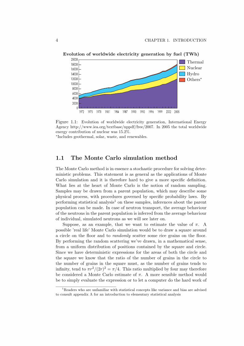
Although somewhat obscured from everyday life, nuclear technology plays animportant role in modern day society. Medical imaging and cancer treat-ment with radiation both rely on nuclides produced in nuclear facilities and ofcourse, a substantial part of worldwide electricity needs is fulfilled by powergenerated in nuclear reactors, see Fig. 1.1. Growing concerns about carbonemissions, slow progress in solar and wind technology and diminishing tradi-tional resources have sparked renewed interest in nuclear energy as a viablealternative to traditional power generation methods for the foreseeable future.
Safety issues are always a major concern when it comes to nuclear facilitiesand having a thorough knowledge of the processes taking place in such facilitiesis therefore a necessity. Because of the risks and high costs involved in runningreal life experiments, nuclear scientists investigating these processes resort tocomputer simulations in most cases. These simulations should of course yieldaccurate results, preferably within as short a time as possible and with a costas low as possible.
While there are many research fields within the nuclear sciences it is thetransport of neutrons in a nuclear reactor core that is key to the way thereactor will behave, and it is the computer simulation of neutron transport,by means of the Monte Carlo technique, this research focuses on.
Besides Monte Carlo there are a number of deterministic methods to simu-late neutron transport. These methods usually involve performing some formof numerical analysis to the equation governing neutron transport and describewhat the neutrons will do on average. Examples are the ’finite elements’ tech-nique [Vermolen, van Kan, and Segal, 2008] or the ’discrete ordinates’ method[Dunderstadt and Hamilton, 1976]. One advantage of these treatments is thatthe solution, if sufficiently accurate, provides full information about the systembeing studied. One disadvantage is that complicated geometries are usuallyhard to handle.
3
4 CHAPTER 1. INTRODUCTION
Evolution of worldwide electricity generation by fuel (TWh)
ThermalNuclearHydroOthers∗
Figure 1.1: Evolution of worldwide electricity generation, International EnergyAgency http://www.iea.org/textbase/nppdf/free/2007. In 2005 the total worldwideenergy contribution of nuclear was 15.2%.∗Includes geothermal, solar, waste, and renewables.
1.1 The Monte Carlo simulation method
The Monte Carlo method is in essence a stochastic procedure for solving deter-ministic problems. This statement is as general as the applications of MonteCarlo simulation and it is therefore hard to give a more specific definition.What lies at the heart of Monte Carlo is the notion of random sampling.Samples may be drawn from a parent population, which may describe somephysical process, with procedures governed by specific probability laws. Byperforming statistical analysis1 on these samples, inferences about the parentpopulation can be made. In case of neutron transport, the average behaviourof the neutrons in the parent population is inferred from the average behaviourof individual, simulated neutrons as we will see later on.
Suppose, as an example, that we want to estimate the value of π. Apossible ’real life’ Monte Carlo simulation would be to draw a square arounda circle on the floor and to randomly scatter some rice grains on the floor.By performing the random scattering we’ve drawn, in a mathematical sense,from a uniform distribution of positions contained by the square and circle.Since we have deterministic expressions for the areas of both the circle andthe square we know that the ratio of the number of grains in the circle tothe number of grains in the square must, as the number of grains tends toinfinity, tend to πr2/(2r)2 = π/4. This ratio multiplied by four may thereforebe considered a Monte Carlo estimate of π. A more sensible method wouldbe to simply evaluate the expression or to let a computer do the hard work of
1Readers who are unfamiliar with statistical concepts like variance and bias are advisedto consult appendix A for an introduction to elementary statistical analysis

1.1. THE MONTE CARLO SIMULATION METHOD 5
counting the rice grains. Two such calculations are shown in Fig. 1.2.Estimating π in this way may seem a lot of work for little gain, and in-
troducing randomness is generally a bad idea when simple problems are con-cerned. It is only when the processes that have to be simulated become verycomplex, as is the case in neutron transport, and the number of dimensionsincreases that Monte Carlo unveils its true potential.
The Monte Carlo method is believed to have been developed at the LosAlamos National Laboratory when computers first made their appearance inthe scientific field. The mathematics of Monte Carlo was however developedat a much earlier stage. The name ”Monte Carlo” was popularized by physicsresearchers Stanislaw Ulam, Enrico Fermi, John von Neumann, and NicholasMetropolis, among others; the name is supposed to be a reference to the MonteCarlo Casino in Monaco where Ulam’s uncle would borrow money to gamble[MacKeown, 1997].
Complicated, real-life processes like neutron transport are usually governedby ’known’ probability laws. In principle it is possible to incorporate thesesame laws in the Monte Carlo simulation. If this is the case we will talk of ananalog simulation; an abstraction of the real life process itself. The conceptualsimplicity of analog simulation may be seen as one of Monte Carlo’s biggestmerits.
On the other hand the probability laws may be wholly artificial; designedfor some specific purpose. Usually it is a mix between the two, because analogsimulation may be very inefficient in some cases. Suppose for example that onewants to study rare events in some system. These rare events will obviouslyalso be rare in the mathematical analog of the system. Vast stores of datamay contain little useful information, leading to a high variance (statistical
−1 −0.5 0 0.5 1−1
−0.5
0
0.5
1
−1 −0.5 0 0.5 1−1
−0.5
0
0.5
1
Figure 1.2: Two Monte Carlo simulations for obtaining an estimate of π are shown.The left figure is for 100 ’rice grains’, leading to an estimate of π = 2.8, and the rightfor 104 grains, leading to an estimate of π = 3.12. A simulation with 109 grains yieldsan estimate of π = 3, 14159, which is close to the real value of π = 3, 14159265..

6 CHAPTER 1. INTRODUCTION
spread) in the estimate following from the simulation. Nothing however pre-vents one from continuing the abstraction by distorting the probability lawssuch that the samples collected during simulation will contain more usefulinformation. The only restriction is that the final estimate should be withoutbias. Simulations containing such modifications will be called non-analog.
Over the years there have evolved a multitude of non-analog techniques inthe Monte Carlo treatment of neutron transport, all of which aim to reducethe variance and/or to boost the efficiency of a simulation. The researcher isleft with the possibility of choosing a strategy for the computation at hand. Inpractice this usually amounts to making decisions by heuristic arguments andby ’rules of thumb’, knowing only after the simulation finishes if the decisionsabout the strategy were truly the right ones.
It turns out that, as will be shown in later chapters, it is possible to calcu-late the variance and efficiency of a particular Monte Carlo simulation strategyfor neutron transport a priori, as opposed to a posteriori (estimated from thesamples collected during simulation). This brings forth the possibility of an-alyzing, comparing and optimizing different strategies before performing theactual simulation and it is exactly that what this research aims to accomplish.
The reason that Monte Carlo simulation has become such a wide spreadtool in nuclear reactors analysis is that it has some advantages over deter-ministic methods. The level of accuracy which can be reached in performingcalculations of some aspects of a reactor is unparalleled. This is largely dueto the fact that, in principle, even very complicated geometries can be usedas an input for the simulation. In deterministic simulations this is simply notpossible due to the complex nature of the equations involved. A Monte Carlosimulation furthermore ’focuses on one aspect’ of the system. For example,the criticality of the reactor or the flux of neutrons in some part of the reactormay be calculated, whereas deterministic simulations provide the solution tothe equations in the entire system and therefore give full information aboutthe problem at hand. Of course, full information may or may not be desirable.Also, Monte Carlo is generally slower than deterministic methods and time-dependent Monte Carlo is still in an infant stage. That’s why both practices,Monte Carlo and deterministic simulations, are in use and are undergoingresearch today.
Details on the mathematical treatment of Monte Carlo for neutron trans-port will follow in chapter 3. If interested in other Monte Carlo methods likequantum Monte Carlo or Monte Carlo for statistical mechanics, the reader isadvised to consult [Thijssen, 2007].
1.2 Scope and goals of this research
This work strives to present and validate both existing and new theory re-garding the a priori calculation of variance and efficiency for Monte Carlo

1.2. SCOPE AND GOALS OF THIS RESEARCH 7
simulations of neutron transport in a way that is complete, readable and haspractical significance.
In order to arrive at such theory, chapter 2 provides an introduction toneutron transport in integral form, suitable for Monte Carlo implementation.Also, concepts like adjoint operators and equations are introduced. Chapter3 deals with the Monte Carlo solution to these transport problems and laysthe foundation, in terms of notation and concepts like scoring and sampling,for later chapters.
In chapter 4, equations necessary for the a priori calculation of variance andefficiency are derived. New theory is introduced regarding the calculation ofthe number of collisions as a measure of computational effort and the variancefor a simulation containing both splitting and Russian roulette. From theexpressions derived in chapter 4, a cost function is constructed which may beminimized to obtain an optimal choice of weight window thresholds. Althoughexpressions are also derived for the more generally used track-length estimator,the emphasis lies on simulations in which the response is estimated using acollision estimator. This yields more appealing results and allows for analyticsolutions more readily.
Chapter 5 provides a number of analytic sample cases to which the theoryis applied. A simplified neutron transport model, in which neutrons are onlyallowed to move in two directions, is introduced. Solutions are provided tothe equations necessary for the minimization of cost.
Chapter 6 then provides specific solutions to the sample cases from chapter5; both a priori, by means of exact analytic solutions, as well as a posteriori, bymeans of estimates from actual Monte Carlo simulations. From the minimumin the cost function an optimal choice of weight window thresholds is obtained.The possibility of source biasing is also explored and verified.
For the practical implementation of the theory presented in this work, itis necessary to be able to solve the equations describing efficiency by means ofexisting deterministic neutron transport codes. Existing codes generally solvean integro-differential transport equation. In chapter 7 it is demonstratedhow the integral equations derived in this work may be transformed into anintegro-differential form that may be suitable.
Since it is the physical nature of the Monte Carlo technique for neutrontransport that is most appealing, the author tries to approach the abstracttheory from an intuitive, physical point of view rather than providing a formalmathematical derivation of all relevant equations. Hopefully this will lead toa readable and even enjoyable work.

Chapter 2
Integral neutron transporttheory
For Monte Carlo purposes, the most common form of the equation describingneutron transport, an integro-differential equation commonly referred to asthe Boltzmann equation [Dunderstadt and Hamilton, 1976], is not well suitedand it is because of this fact that the transition is made to describing neutrontransport in a purely integral form. The following sections provide an intro-duction to this integral neutron transport theory; emphasizing the physicalnature of the processes involved while doing so. This will prove convenientwhen making the transition to the more abstract theory treated in chapter4. Also, concepts from adjoint theory will be presented and the necessarynotation will be introduced.
2.1 Preliminaries
To fully describe a neutron in a mathematical sense, one would need its posi-tion in space r, its velocity v and its point in time t. In nuclear reactor physicsit has become customary to adopt more convenient variables, although entirelyequivalent, for the velocity of the neutron. The velocity vector is essentiallydecomposed into two components; one characterizing the neutron speed andthe second the direction of motion of the neutron.The speed is characterized by the kinetic energy of the neutron
E =12m|v|2 (2.1)
The direction is characterized by a unit vector in the direction of motion ofthe neutron
Ω =v
|v|(2.2)
9

10 CHAPTER 2. INTEGRAL NEUTRON TRANSPORT THEORY
A point in the phase space will from now on be represented as follows
P = (r,Ω, E) (2.3)
in which the time variable t is left out here because Monte Carlo calculationsare mainly concerned with stationary problems.
The variable that is most commonly used in nuclear reactor physics is theangular neutron flux
φ(P ) =the number of neutrons per unit energy rangeand unit solid angle passing through a surfacewith normal Ω at P
In nuclear reactor calculations one is generally interested in some physicalproperty of the system, like the flux of neutrons in some part of the reactor orthe dose rate in some volume of material. We shall call this quantity R andrefer to it as the detector response. Formally, R is a functional or weightedintegral of some response or payoff function η(P ) and a solution function φ(P ).
R =∫η(P )φ(P )dP (2.4)
The solution function φ(P ) may be the angular neutron flux. The payofffunction η(P ) then determines what the integral represents.
Cross sections
A concept of importance in nuclear reactor theory is that of cross sections;see [Bell and Glasstone, 1970] or [Dunderstadt and Hamilton, 1976] for a fullaccount. One can define the microscopic cross section σ [cm2] as
σ =Number of reactions/nucleus/sec
Number of incident neutrons/cm2/sec(2.5)
The total microscopic cross section σt represents the sum over all cross sectionsof some interaction type, here denoted by the subscript j. j may for examplerepresent elastic scattering, inelastic scattering, fission, or any other distinctinteraction.
σt =∑j
σj = σe + σin + σnα + ... (2.6)
We define the absorption cross section to characterize any event other thanscattering (also including fission)
σa = σt − σs (2.7)
For the purposes of this thesis it is more convenient to abandon the conceptof the microscopic cross section and adopt the macroscopic cross section Σ

2.2. INTEGRAL TRANSPORT EQUATIONS 11
[cm−1] as the characterization of interaction types. If the matter consists ofcomponents denoted by subscript A, then the total macroscopic cross sectionis the weighted sum of the microscopic cross sections of interaction type j andcomponent A
Σt(r, E) =∑A
NA(r)∑j
σj,A(E) (2.8)
in which NA(r) represents the atomic number density of nuclide A and σj,A(E)denotes the microscopic cross section of interaction type j, provided nuclideA. Note that the macroscopic cross section is written as a function of spaceand energy and not of direction. For practically all applications in nuclearreactor analysis this simplification holds. For notational convenience how-ever, we might sometimes write Σt(P ). The macroscopic total cross sectionΣt represents the probability of interaction per unit distance traveled. Thereciprocal of this quantity is therefore the neutron mean free path. We canease notation even further by introducing a partial macroscopic cross section
Σj,A(r, E) = NA(r)σj,A(E) (2.9)
with which Eq. (2.8) reduces to
Σt(r, E) =∑A
∑j
Σj,A(r, E) (2.10)
In case of an interaction, the particle may undergo a change in directionand energy. For neutrons with direction Ω′ and energy E′ we define thedifferential cross section as
Σj(r,Ω′ → Ω, E′ → E) = Σj(r, E′)pj(Ω′ → Ω, E′ → E) (2.11)
in which pj(Ω′ → Ω, E′ → E)dΩdE represents the probability that the neu-tron coming out of the interaction of type j has a direction Ω in dΩ andenergy E in dE. For elastic scattering this probability is normalized to unity.
To incorporate fission we introduce ν(r, E) as the average number of neu-trons produced by a fission at r caused by a neutron of energy E. The criti-cality of a reactor can be conveniently defined as
keff =Number of neutrons in generation i+ 1
Number of neutrons in generation i(2.12)
2.2 Integral transport equations
The equation describing neutron transport most common to nuclear physicistsis the stationary Boltzmann transport equation
Ω · ∇φ(P ) + Σt(r, E)φ(P )
=∫
4π
∫Σs(r, E′ → E,Ω′ → Ω)φ(r, E′,Ω′)dE′dΩ′ + S(P ) (2.13)

12 CHAPTER 2. INTEGRAL NEUTRON TRANSPORT THEORY
It is possible to transform Eq. (2.13) into a purely integral equation whichis suitable for Monte Carlo implementation, [Bell and Glasstone, 1970], thederivation of which will be treated in chapter 7 and is of no particular interestat this point. Rather, following an intuitive approach to find the integralequation describing neutron transport will provide the necessary insight intothe relevant physical processes. To that end let us first introduce the collisiondensity of neutrons at a point in phase space
ψ(P ) =the number of neutrons per unit volume,unit energy range and unit solid angleentering a collision at P
The collision density is related to the angular neutron flux via a simple relation
ψ(P ) = Σt(P )φ(P ) (2.14)
From Eq. (2.14) it becomes clear that in vacuum there will be no interactionso the collision density is zero, whatever value the neutron flux might be.
Somewhat equivalently it is possible to define an emission density of neu-trons
χ(P ) =the number of neutrons per unit volume,unit energy range and unit solid anglestarting a flight path at P
Several physical processes may provide the neutrons that constitute the emis-sion and collision densities. There may be a source S(P ) of neutrons
S(r,Ω, E) = S(P ) (2.15)
Neutrons may make a transition to a new collision site, a process which canbe described by the transition kernel T (r′ → r, E,Ω), in which
T (r′ → r, E,Ω)dV =the probability for a neutron starting at r′,with energy E and direction Ωto have its next collision in dV at r.
The general form of T in three dimensions, [Lux and Koblinger, 1991], is givenby
T (r′ → r, E,Ω)
= Σt(r, E)exp
−∫ |r−r′|
0Σt(r − sΩ, E)ds
δ(Ω− r−r′
|r−r′|)
|r − r′|2(2.16)
in which s = |r − r′| represents the path length between two collision pointsr and r′. T is normalized to unity for an infinite system. For a finite system
2.2. INTEGRAL TRANSPORT EQUATIONS 13
we can circumvent the normalization ’problem’ by imagining the system beingsurrounded by a purely absorbing medium so that we can take the integral overthe entire space volume. Neutrons are simply killed when exiting the system.The transition kernel can thus be understood as a conditional probabilitydensity function for a new collision site r, given r′, E,Ω.
At this point it should be noted that, although time dependence was omit-ted it can be easily implemented, since if a neutron travels a distance |r− r′|with speed v =
√2E/m, the time increase will simply be |r − r′|/v.
Neutrons in the system may also enter a collision and undergo a changein direction and energy. The collision kernel C(r, E′ → E,Ω′ → Ω) describesthis process;
C(r, E′ → E,Ω′ → Ω)dEdΩ =
the probability for a neutronentering a collision at r′
with energy E′ and direction Ω′
to exit the collision with energyE in dE and direction Ω in dΩ
In general form, the collision kernel can be written as, [Hoogenboom, 1977]
C(r, E′ → E,Ω′ → Ω)
=∑A
∑j
pj,A(r, E′)cj,A(E′)pj,A(E′ → E,Ω′ → Ω) (2.17)
in which pj,A(r, E′) represents the conditional probability of an interactiontype j provided a collision with nuclide A
pj,A(r, E′) =Σj,A(r, E′)Σt(r, E′)
(2.18)
and cj,A(E′) represents the average number of neutrons released in a collisiontype j with a nuclide A. In case of scattering, cs,A(E′) = 1; in case of fissionthe number of neutrons released will be equal to ν(E′).pj,A(E′ → E,Ω′ → Ω) represents the joint transfer probability for (E′ → E)and (Ω′ → Ω) given collision type j with nuclide A. Except for an absorptionevent this probability is normalized to unity.
The collision density ψ(P ) is related to the emission density in the followingway
ψ(P ) =∫T (r′ → r, E,Ω)χ(r′, E,Ω)dV ′ (2.19)
as the density of neutrons entering a collision at r with direction Ω and energyE is formed by the density of neutrons starting a flight at r′ with direction Ωand energy E, traveling to r. Alternatively, one can write a relation for theemission density
χ(P ) = S(P ) +∫ ∞
0
∫4πC(r, E′ → E,Ω′ → Ω)ψ(r, E′,Ω′)dE′dΩ′ (2.20)
14 CHAPTER 2. INTEGRAL NEUTRON TRANSPORT THEORY
Note that the emission density represents the right hand side of the Boltmannequation, Eq. (2.13).
Using Eq. (2.20) to rewrite Eq. (2.19), one arrives at the transport equa-tion for the collision density ψ(P )
ψ(P ) = S1(P ) +∫K(P ′ → P )ψ(P ′)dP ′ (2.21)
in which S1(P ) represents the source of first collisions
S1(P ) =∫VT (r′ → r, E,Ω)S(r′, E,Ω)dV ′ (2.22)
and K(P ′ → P ) represents the transport kernel for the collision density
K(P ′ → P ) = C(r′, E′ → E,Ω′ → Ω)T (r′ → r, E,Ω) (2.23)
Eq. (2.21) is a so-called Fredholm type integral equation of the second kind[Pipkin, 1991] which will be of particular interest for the Monte Carlo so-lution procedure discussed in chapter 3. The transport kernel K(P ′ → P )represents the probability for a neutron with energy E′ and direction Ω′ en-tering a collision at r′, to have a change in energy and direction to E and Ωand subsequently have a free flight to r.
Along the same lines as for the collision density one can derive the trans-port equation for the emission density χ(P )
χ(P ) = S(P ) +∫L(P ′ → P )χ(P ′)dP ′ (2.24)
in which S(P ) represents the true source density and L(P ′ → P ) representsthe transport kernel for the emission density
L(P ′ → P ) = T (r′ → r, E′,Ω′)C(r, E′ → E,Ω′ → Ω) (2.25)
It is interesting to note here the difference between the two transport kernels.L(P ′ → P ) implies first having a flight from r′ to r with energy E′ anddirection Ω′ and subsequently a collision at r to have a change in energy toE and a change in direction to Ω. K(P ′ → P ) implies first having a collisionat r′ resulting in a change in energy to E and a change in direction to Ω andsubsequently the flight from r′ to r but now, of course, with energy E anddirection Ω.
The detector response can now be expressed in terms of any of the threefunctions encountered in this section
R =∫ηφ(P )φ(P ) =
∫ηψ(P )ψ(P ) =
∫ηχ(P )χ(P ) (2.26)
The interrelations between the different payoff functions ηφ(P ), ηψ(P ) andηχ(P ) will be treated shortly.

2.3. ADJOINT THEORY 15
2.3 Adjoint theory
Adjoint equations and adjoint operators play an important role in the math-ematical analysis of complex systems. For the remainder of this work someconcepts from adjoint theory will be essential and are therefore briefly dis-cussed below.Suppose we write Eq. (2.21) in operator form as
Aψ(P ) = S1(P ) (2.27)
We shall call this the forward equation. We then proceed to define the equationadjoint to Eq. (2.27) as
A∗ψ∗(P ) = S∗1(P ) (2.28)
in which we recognize three quantities: the adjoint transport operator A∗, anadjoint source term S∗1(P ) and of course the solution to the adjoint equationψ∗(P ).
The definition of the adjoint operator A∗ follows from a commutative re-lation. Suppose f(P ) and g(P ) are two arbitrary elements in the domain ofsome operator B, the adjoint operator then obeys∫
f(P )Bg(P )dP =∫g(P )B∗f(P )dP (2.29)
Finding the adjoint of an operator often involves deriving adjoint boundaryconditions (details can be found in [Ronen, 1986]). As a simple examplesuppose B represents the product operator. In that case obviously B∗ = B,no adjoint boundary conditions need to be specified and we proceed to callthe product operator self-adjoint.As another example consider the integral operator
Kg(P ) =∫K(P ′ → P )g(P ′)dP ′
We see from Eq. (2.29) that∫f(P )Kg(P )dP =
∫ ∫f(P )K(P ′ → P )g(P ′)dP ′dP
=∫g(P ′)
∫K(P ′ → P )f(P )dPdP ′
switch P to P ′ and vice versa
=∫ ∫
g(P )K(P → P ′)f(P ′)dP ′dP =∫g(P )K∗f(P )dP
and therefore
K∗f(P ) =∫K(P → P ′)f(P ′)dP ′ (2.30)

16 CHAPTER 2. INTEGRAL NEUTRON TRANSPORT THEORY
Taking the adjoint of an integral operator transposes the kernel.What remains is finding a suitable adjoint source term S∗1(P ). With suit-
able in this case we mean that the solution to the adjoint equation shouldrepresent something that can aid in solving the forward problem. Now recallthat the aim of a calculation was to obtain a detector response, written hereas a weighted integral over the collision density
R =∫ηψ(P )ψ(P )dP (2.31)
in which ηψ(P ) is recognized as the payoff function with respect to the collisiondensity ψ(P ). Now multiply the forward transport equation, Eq. (2.27), withψ∗(P ) and the adjoint equation, Eq. (2.28), with ψ(P ) and integrate over thewhole phase space.∫
ψ∗(P )Aψ(P )dP =∫ψ∗(P )S1(P )dP∫
ψ(P )A∗ψ∗(P )dP =∫ψ(P )S∗1(P )dP (2.32)
Taking the adjoint source S∗1(P ) equal to ηψ(P ), the following relation isobtained
R =∫ηψ(P )ψ(P )dP =
∫S1(P )ψ∗(P )dP (2.33)
which shows that, given this adjoint source definition, ψ∗(P ) may be inter-preted as the importance or expected contribution to the detector responseof a particle entering a collision at P . Integration of this function over thedensity of first collisions returns the detector response.
Returning to the usual notation we write the transport equation for ψ∗(P )as
ψ∗(P ) = ηψ(P ) +∫K(P → P ′)ψ∗(P ′)dP ′ (2.34)
which again is a Fredholm type integral equation of the second kind, muchlike the forward equation. In this case, however, the payoff function ηψ(P )acts as a source density and transport is governed by the transposed kernel
K(P → P ′) = C(r, E → E′,Ω→ Ω′)T (r → r′, E′,Ω′) (2.35)
Because the forward and adjoint equations are so closely related the MonteCarlo treatment of forward and adjoint transport is for a great part the same,albeit, in the case of adjoint transport, some extra interpretation of the kernelis necessary. For example, a collision of an adjoint ’pseudo’ particle will usuallylead to an increase in energy. The Monte Carlo treatment of forward neutron
2.3. ADJOINT THEORY 17
transport will be treated in chapter 3 and adjoint transport will be covered inappendix B.
The equation adjoint to Eq. (2.24) is written as
χ∗(P ) = ηχ(P ) +∫L(P → P ′)χ∗(P ′)dP ′ (2.36)
and the response is expressed as
R =∫ηχ(P )χ(P )dP =
∫S(P )χ∗(P )dP (2.37)
χ∗(P ) represents the importance or expected contribution to the detectorresponse of a neutron starting a flight path at P . The transposed kernelL(P → P ′) can be written out explicitly
L(P → P ′) = T (r → r′, E,Ω)C(r′, E → E′,Ω→ Ω′) (2.38)
Some other relations between the various relevant functions can be derived.If one substitutes Eq. (2.19) in Eq. (2.31), interchange integration variablesand use Eq. (2.37) one finds
R =∫Pηψ(P )
∫VT (r′ → r, E,Ω)χ(r′, E,Ω)dV ′dP
switch r to r′ and vice versa
=∫P
∫Vηψ(r′, E,Ω)T (r → r′, E,Ω)χ(P )dV ′dP
=∫ηχ(P )χ(P )dP
and, given that this holds for any χ(P ), therefore
ηχ(P ) =∫T (r → r′, E,Ω)ηψ(r′, E,Ω)dV ′ (2.39)
Another useful relation between the payoff functions can be derived fromEq. (2.14). Because
R =∫ηφ(P )φ(P )dP =
∫ηφ(P )
ψ(P )Σt(P )
dP =∫ηψ(P )ψ(P )dP
we have
ηψ(P ) =1
Σt(P )ηφ(P ) (2.40)
To arrive at a relation between the different adjoint functions, multiplyEq. (2.34), using r′ in stead of r, with T (r → r′, E,Ω) and integrate over r′
18 CHAPTER 2. INTEGRAL NEUTRON TRANSPORT THEORY
to obtain ∫T (r → r′, E,Ω)ψ∗(r′, E,Ω)dV ′ = ηχ(P )+∫
L(P → P ′)∫T (r′ → r′′, E′,Ω′)ψ∗(r′′, E′,Ω′)dV ′′dP ′
and compare with Eq. (2.36) to see that
χ∗(P ) =∫T (r → r′, E,Ω)ψ∗(r′, E,Ω)dV ′ (2.41)
using Eq. (2.41) in Eq. (2.34) one finds that
ψ∗(P ) = ηψ(P ) +∫ ∫
C(r, E → E′,Ω→ Ω′)χ∗(r, E′,Ω′)dE′dΩ′ (2.42)
As a final way of expressing the response we write
R =∫φ(P )ηφ(P )dP =
∫S(P )φ∗(P )dP (2.43)
and note that the importance functions φ∗(P ) and χ∗(P ) are the same. Bothrepresent the importance or expected contribution to the detector response ofa neutron starting a flight at P .
This concludes the derivation of the relevant transport equations and theirinterrelations. Later on in chapter 4 we will encounter even more, and morecomplicated, transport equations for processes closely related to the collisionand emission densities and the foundations laid in this chapter will be used tomanipulate these equations.

Chapter 3
Monte Carlo for neutrontransport
In this chapter, a brief description of the process of Monte Carlo simulationwith respect to neutron transport will be given. The derivation will again befrom an intuitive, physical point of view rather than providing the rigorousmathematical formalism that underlies the Monte Carlo method. For sucha rigorous treatment the reader is advised to consult [Spanier and Gelbard,1969].
Monte Carlo simulation relies heavily on statistical tools. Appendix Atherefore deals with a basic introduction to statistics and estimation, intro-ducing some notation on the fly. Readers who have experience in the fieldmay proceed directly to section 3.1 which covers the mathematical formalismof the Monte Carlo procedure along the lines of [Hoogenboom, 1977] and [Luxand Koblinger, 1991]. Appendix B explains how adjoint transport may beaccomplished by means of Monte Carlo.
3.1 The theoretical framework of Monte Carlo
Now that the necessary statistical tools, the mathematical description of for-ward and adjoint transport and the basic ideas behind Monte Carlo simulationhave been discussed it is time to cast everything into a formalism which canbe employed in computer simulation.
The goal of a simulation is to obtain an estimate of the response R. Toillustrate how this can be accomplished by means of Monte Carlo consider thefollowing example. Suppose one is interested in the average of a known func-tion ϕ(x) over some interval [a, b] in a one-dimensional system. The responsecan in that case be written as
R =1
b− a
∫ b
aϕ(x)dx
19

20 CHAPTER 3. MONTE CARLO FOR NEUTRON TRANSPORT
Now we could of course estimate the integral, which represents the area belowthe graph of ϕ(x), in the same way as we could estimate the value of π; i.e.we could randomly select points in a rectangle containing the function ϕ(x),check the ratio of points below and above the graph, and from this ratio obtainan estimate of the area. There is another method, however, which requiresless effort. The integral can also be estimated by
R =1N
N∑i=1
ϕ(xi) (3.1)
with the position variable taken randomly from a uniform distribution onthe interval [a, b]. The random selection of position, which can be achievedby sampling the uniform pdf for positions by generating a random numberin a computer, makes it a Monte Carlo simulation. It will be clear that Rwill provide a reasonable and unbiased estimate, provided that the number ofsamples N is large enough.
The above methods are of course not very enlightening for neutron trans-port since they assume the function ϕ(x) to be known. This is for mostpurposes never the case, since we would then simply evaluate the integral andbe done with it. Rather, one has to obtain an estimate of the solution to thetransport equation governing neutron transport as well. So generally, in orderto obtain an estimate of the response, we will need to estimate the solutionfunction by means of random numbers.
The solution functions encountered in chapter 2 were defined by type twoFredholm integral equations with kernels K(P ′ → P ), L(P ′ → P ) and theiradjoint counterparts. These equations have a solution in terms of a seriesdevelopment. Consider for example the solution to the emission density, Eq.(2.24), expressed as an infinite Neumann series expansion, [Pipkin, 1991]
χ(P ) =∞∑i=0
χi(P ) (3.2)
χ0(P ) = S(P )
χ1(P ) =∫L(P ′ → P )S(P ′)dP ′
χ2(P ) =∫ ∫
L(P ′ → P )L(P ′′ → P ′)S(P ′′)dP ′′dP ′
This solution converges uniformly, provided that the transport kernel is bounded‖L‖2 < 1 with ‖L‖ = sup
∫ ba | L(P ′ → P ) | dP ′ and non-negative. These con-
ditions are satisfied in the case of neutron transport for a non-fissile system.The Monte Carlo solution of Eq. (3.2) then turns out to be remarkably in-tuitive from a physical point of view (as it should be, since it represents ananalog of the physical reality).

3.1. THE THEORETICAL FRAMEWORK OF MONTE CARLO 21
From Eq. (3.2) it becomes clear that the emission density at P may beconsidered as being comprised of neutrons coming from other ’source’ points(P ′, P ′′, P ′′′, ...), traveling eventually to P and starting a flight there. In thisinterpretation, each emission (either from a source or after a collision event)of a neutron during its lifetime at a point in phase space constitutes a sampleof the emission density at that point in phase space. Since S(P ) and thekernel L(P → P ′) represent probability densities, the Monte Carlo procedurewould involve tracking such a neutron history by randomly sampling the sourcedensity S(P ′) for a birth point P ′ and randomly sampling the transport kernelL(P ′ → P ) for new emission points. One is effectively sampling the probabilityspace of neutron ’random walks’; terminology often used in this context.
Following the random walks, or histories, of a large number of neutronsand saving the emission sites results in an estimate of the emission densityfunction in the system.
The series development can also be done for the detector response in termsof the emission density
R =∞∑j=0
Rj =∫ηχ(P )S(P )dP (3.3)
+∫ηχ(P )
∫L(P ′ → P )S(P ′)dP ′dP + ...
From Eq. (3.3) it now becomes clear that ’scoring’ ηχ(Pj) at every emissionsite Pj in a neutron history and subsequently summing all these scores leadsto a sample or estimate of R.
Scores can also be collected when a particle enters a collision, in whichcase the scoring function is the payoff function for the collision density: ηψ(P ).From Eq. (2.20) and Eq. (2.22) it follows that we actually have a coupledsystem of equations
χ0(P ) = S(P )
ψ0(P ) =∫T (r′ → r, E,Ω)χ0(r′, E,Ω)dV ′
i+ 1 = 1, 2, ...,∞
χi+1(P ) =∫C(r, E′ → E,Ω′ → Ω)ψi(r, E′,Ω′)dE′dΩ′
ψi+1(P ) =∫T (r′ → r, E,Ω)χi+1(r′, E,Ω)dV ′
Source points can be sampled from a pdf which describes the source densityS(P ). A new position is selected from the transition kernel, which representsa conditional pdf for r given r′. This new point represents the first sampleof the collision density and a score with respect to the response estimate maybe saved here. A new emission point may be randomly selected from the

22 CHAPTER 3. MONTE CARLO FOR NEUTRON TRANSPORT
S
T
C
χ
ψ
Figure 3.1: A schematic representation of the Monte Carlo treatment of neutrontransport showing the positions at which different quantities are obtained and sampledduring a neutron history.
collision kernel where a score may also be saved, and so forth. A schematicrepresentation of the formalism is shown in Fig. 3.1 and the appropriatemathematical treatment of analog Monte Carlo is summarized in Table 3.1.The response estimate is then constructed from the scores gathered with the
Do for N neutrons from j = 1...Nset i = 0 and proceed until leakage or absorption
1: Sample S(P ) for initial coordinates (r0, E0,Ω0)2: Possibly score ηχ(Pi) at an emission3: Sample T (ri → ri+1, Ei,Ωi) for next collision site ri+1
4: Possibly score ηψ(ri+1, Ei,Ωi) at a collision5: Sample C(ri+1, Ei → Ei+1,Ωi → Ωi+1) for (Ei+1,Ωi+1)
Set Pi = (ri+1, Ei+1,Ωi+1) and return to 2:Determine Rj from the score collected during history jand proceed with the next neutron history
Table 3.1: Monte Carlo procedure for analog neutron transport
appropriate scoring function during the individual neutron histories: Rj , withj = 1..N
R =1N
N∑j=1
Rj (3.4)
and in which N represents the number of neutron histories. The scoring func-tions ηψ and ηχ can be as diverse as the physical quantities to be determined.Sometimes there are even multiple possibilities for estimation of a certainquantity. The most common estimators are the collision estimator and the

3.1. THE THEORETICAL FRAMEWORK OF MONTE CARLO 23
track length estimator. Both will be treated in chapter 4. As an example,suppose one is interested in the average flux in some detector volume Vdet.The response can in that case be written as
R =1Vdet
∫ ∫ ∫Vdet
φ(P )dV dEdΩ =1Vdet
∫ ∫ ∫Vdet
ψ(P )Σt(P )
dV dEdΩ
from which the appropriate scoring function is obtained
ηψ(P ) =1
VdetΣt(P )r ∈ Vdet
Every time a neutron enters a collision in the detector volume Vdet, a scoreor tally ηψ(P ) is recorded and the response is calculated from all scores, callthem si, gathered during all histories as
R =1N
∑i
si (3.5)
The statistical tools stated in appendix A apply to a response estimate R.Obviously, due to the law of large numbers, increasing the number of neutronhistories N will lead to a better estimate with lower variance in the mean. Onthe other hand this will lead to longer computation times. These criteria canbe summarized in the Figure Of Merit or FOM, [Lux and Koblinger, 1991]
FOM =1
TVar(R)(3.6)
in which T represents the time the calculation took and Var(R) is the relativevariance, Eq. (A.7).
Both quantities scale with the number of neutron histories N , which makesthe FOM roughly independent of this number. Any non-analog simulationstrategy should strive to attain a higher FOM (or to a lower variance depend-ing on ones preference). Since the FOM is calculated from the simulationdata, one only knows afterwards if this goal is achieved.
In chapter 4 a cost function is defined as the product of the expected vari-ance and the expected number of collisions resulting from a neutron history.It can be interpreted as the inverse of the figure of merit and as it can becalculated a priori, without performing a simulation, provides one with a toolto compare, analyze and even optimize simulation strategies.
A little extra information on the actual sampling of probability distribu-tions like the transition kernel is required before proceeding with modificationsof analog transport.

24 CHAPTER 3. MONTE CARLO FOR NEUTRON TRANSPORT
Sampling probability distributions
Monte Carlo simulation relies on computer generated random1 numbers, de-noted by ρ from this point on, for the sampling of probability distributions.There are numerous ways to perform the actual sampling and as it is notan essential part of this research we will treat two simple examples here andrefer the reader to [Lux and Koblinger, 1991] for a full treatment of differentpossibilities. ρ has a uniform distribution between 0 and 1
Prob(ρ ≤ x) =∫ x
0dx′ x ∈ (0, 1) (3.7)
Suppose a neutron starts a flight and we want to sample the transition kernel,Eq. (2.16), for a new collision site. In a homogeneous system the track lengths = |r′ − r| has a probability distribution according to Σte
−Σts s ∈ [0,∞).We can relate the computer generated random number to the track-length inthe following way
ρ = P (t) =∫ s
0Σte−Σts′ds′ → s =
ln(1− ρ)Σt
≡ − ln(ρ)Σt
This technique is commonly known as the inverse probability method. Obvi-ously in a non-uniform system the expressions become more complicated.
Another easy example is sampling the collision kernel, Eq. (2.17), in auniform system where the neutrons are only allowed to move in the positive→, or negative ← directions. The collision outcomes are either absorption(leading to termination of the neutron) or scattering, and energy dependenceis omitted. The scattering cross section is then formed by the partial crosssections for the positive and negative directions: Σs = Σ→ + Σ←
The interaction probability under these restrictions is simply pj = Σj/Σt
from which it follows that
j = a if ρ ≤ Σa/Σt
j = s otherwise
and, given a scattering event, the probability to scatter ps(Ω′ → Ω) in eitherone of the two directions, irrespective of the incoming direction, is given by
Ω =→ if ρ ≤ Σ→/Σs
Ω =← otherwise
For more complex probability distributions, obtaining expressions like theabove is usually not that simple.Now that all the tools are available to perform forward, analog simulations itis time to address possible modifications of the analog game.
1Computer generated random numbers are never truly random but with current tech-niques, for all intents and purposes they are. If true randomness is required, one can forexample use random numbers generated from atmospheric noise. It is however very unlikelythat the computer generated numbers will not suffice.

3.2. MODIFICATIONS OF THE ANALOG GAME 25
3.2 Modifications of the analog game
As mentioned in the introduction, from a mathematical point of view it doesn’tmatter how one distorts the probability laws governing the analog transport ofneutron transport, as long as the resulting Monte Carlo estimate will representthe desired response without bias.
The idea behind modification of the analog game in the context of neutrontransport stems from the fact that many particles may never contribute or maycarry little significance with respect to the intended response estimate; theymay be absorbed or leak long before entering a region of phase space where ascore may be recorded. To get an estimate with a reasonable variance in sucha situation would involve simulating large amounts of particles, which in turnresults in large computing times.
There are a number of ways in which the analog game can be modified,but basically all rely on the possibility to assign a statistical weight W as anextra variable to a particle to account for not sampling the analog probabilitydistribution (pdf) of the respective process. The weight ensures that the finalestimate will be unbiased. In analog simulations the particles will always carrya weight equal to one, but this restriction is left out here in light of applicationslater on. In general, to obtain an unbiased estimate of R, we require
W × pdf = W × pdf (3.8)
in which the overline represents the modified situation.Three modifications of the analog game most common to neutron transport
will be discussed below. Their implications with respect to the variance andefficiency of a simulation will be examined further in chapters 4 and 5.
Implicit Capture
The most intuitive and commonly used form of modification is implicit cap-ture. Whenever a particle collides, the possibility of absorption is accountedfor by multiplying the statistical weightW of the particle by the non-absorptionprobability κ(P ) = Σs(P )/Σt(P ). So in stead of possibly terminating a his-tory at collision point P due to absorption, the collision kernel is distortedand the weight is altered according to
W ′ = Wκ(P ) κ(P ) ≤ 1
If a detector is located at P and the particle, born with W = 1, has hadk collisions at sites (P0, P1...Pk) before scoring at P , the score will be equalto κ(P0)κ(P1)...κ(Pk)η(P ), whereas the score would have been zero with agreater probability for an analog simulation. Implicit capture therefore re-duces variance but increases computational time. Exactly how these effectswill manifest themselves mathematically is treated in chapter 4.
26 CHAPTER 3. MONTE CARLO FOR NEUTRON TRANSPORT
Russian roulette and Splitting
Russian roulette is introduced as a means of terminating particles that carrya low statistical weight in order to improve the efficiency of a simulation;increasing variance but decreasing computational effort. If the particle weightW at P is below some threshold W ≤ Wth(P ), the Russian roulette game isplayed in which case the particle either survives the game with probabilityz1(P ) and gets assigned a new survival weight Ws(P ), or the particle getskilled with probability z0(P ) = 1− z1(P ). In order to have a statistically fairgame it is required that the expected weight after a Russian roulette event isequal to W i.e. z1(P )Ws(P ) + (1− z1(P ))0 = W or z1(P ) = W/Ws(P )
As opposed to terminating particles with low statistical weight by means ofRussian roulette, it is common practice to ’split’ particles with a weight higherthan some user defined threshold weight Wsplit(P ) into a number of identi-cal particles in order to increase the probability of scoring. This procedureis called splitting and usually both procedures are implemented in so-calledweight windows. The weight window boundaries that define the window maybe space and energy dependent and choosing them correctly can significantlyimprove simulations. The modification of the weight is slightly different inthis case
NsplitW′ = W (3.9)
in which Nsplit represents the number of split particles and W ′ represents theweigh of the identical particles emerging from the splitting event.
Setting these weight window boundaries in practice usually boils downto performing educated guesses or using iterative methods. A theoreticaltreatment of how exactly these windows affect the variance and efficiency ofa simulation is given in chapter 4 and in chapter 5 some sample cases arestudied to examine how this theory can be applied to optimize the choice ofweight window thresholds a priori.
Source biasing
The idea behind source biasing stems from the fact that there may very wellbe source regions in phase space which are of low importance with respect tothe response. Suppose for example that detection is done in a small regionof a highly absorbing system and that the source is located throughout thesystem. Particles that have to travel a long distance to reach the detector willhave a low probability of scoring a significant amount in any case. In such asituation it will be favorable to bias the spatial distribution of the source suchthat more particles will be born close to the detector region.
The way in which source biasing is usually implemented in practice, isthat the physical source density is biased with the adjoint flux φ∗(P ) in the

3.2. MODIFICATIONS OF THE ANALOG GAME 27
following way, [Haghighat and Wagner, 2003]
S(P ) =φ∗(P )S(P )∫φ∗(P )S(P )dP
=φ∗(P )S(P )
R
in which the adjoint function and the response may be approximated by anexisting, deterministic neutron transport code.
Although φ∗(P ) seems a likely candidate for ’optimal source biasing’, asit represents the importance of a particle starting a flight, it remains unclearwhether it will give the best result in every situation. There is for example alsothe adjoint function ψ∗(P ) which may yield better results in some cases, ormaybe some other function. Let us therefore state a general biasing functionΓ(P ) and implement biasing as
S(P ) =Γ(P )S(P )∫Γ(P )S(P )dP
(3.10)
The modified initial neutron weight will then be equal to
W (P ) = W
∫Γ(P )S(P )dP
Γ(P )(3.11)
The tools presented in chapter 4 provide the possibility to investigate an op-timal choice for a biasing function.
Another ’rule of thumb’ that seems to pay off in practice is to let the biasedinitial weight of the source particle determine the bounds of the weight window(containing both Russian roulette and splitting). The idea is, according to[Haghighat and Wagner, 2003], that a source particle should neither split norplay Russian roulette immediately, and therefore that the biased initial weightshould be located midway between both thresholds in the window.
W (P ) =Wsplit(P ) +Wth(P )
2
and therefore
Wth(P ) ≡W∫
Γ(P )S(P )dPΓ(P )
(β + 1
2
)−1
(3.12)
in which β = Wsplit(P )/Wth(P ) is the ratio of the upper and lower bounds ofthe weight window. The default value for β in the general purpose Monte Carlocode MCNP is 5, [Laboratories, 2008], and it is observed that the efficiency isfairly insensitive to small deviations from this number.
These rules of thumb all makes sense from an intuitive perspective, butthe tools presented in chapter 4 now also provide the possibility to investigatewhether or not they provide the best possible result.
To complete the treatment of Monte Carlo for neutron transport, appendixB deals with adjoint Monte Carlo. The equations for variance and efficiency,

28 CHAPTER 3. MONTE CARLO FOR NEUTRON TRANSPORT
derived in the following chapter, are generally adjoint equations which in prin-ciple can be solved by means of the Monte Carlo formalism explained there;albeit some extra modifications will be necessary due to modified transportprobabilities.

Chapter 4
Theoretical calculation ofvariance and efficiency
The efficiency of a neutron transport Monte Carlo simulation is measured bythe FOM, Eq. (3.6). For the a priori calculation of efficiency it is there-fore necessary to arrive at measures for both the variance and computationaltime of the simulation. As we will see, both can be achieved by exploiting apowerful insight. The score collected during a neutron history is itself prob-abilistic and therefore has an associated probability score distribution. Fromthis distribution so called moment equations can be constructed, from whichthe expected variance of a simulation can be obtained.
It turns out to be important where to start the derivation. From Table3.1 it becomes clear that there are two distinct events during the simulationof a neutron; the start of a neutron flight (following a collision or birth) ora collision event. The notion of a probability score distribution is borrowedfrom [Lux and Koblinger, 1991], who applied it to a neutron starting a flightand who followed a rigorous and general mathematical approach.
It turns out that looking at a neutron entering a collision yields more ap-pealing results when using a collision estimator. This insight was first putforward by [Hoogenboom, 2004], who derived an equation describing the vari-ance for a simulation with Russian roulette (without using the concept of aprobability score distribution). The theory presented in the following maybe seen as an extension to the work of both [Lux and Koblinger, 1991] and[Hoogenboom, 2004].
The emphasis lies on simulations using the collisions estimator for obtain-ing a response estimate because the equations then allow for exact analyticsolutions in some cases more readily.
To give a consistent and readable treatment, first an equation for the vari-ance of an analog simulation is derived. Once the concept and necessarynotation is sufficiently clear, the transition is made to non-analog games. The
29

30CHAPTER 4. THEORETICAL CALCULATION OF VARIANCE AND
EFFICIENCY
most common of which, using implicit capture to reduce variance in the es-timate, is treated in section 4.2. In section 4.3 expressions are derived forthe variance of a simulation when both Russian roulette and splitting are ap-plied in a weight window. This requires some new theory to be introduced toaccount for the splitting procedure.
To estimate the computational time of a simulation, some new theoryconcerning the estimation of the number of collisions during a particle historyis introduced in section 4.4. From the number of collisions and variance, thecost function is constructed which may be minimized to obtain an optimalchoice of weight window thresholds and optimal source biasing functions.
In order to give a full treatment, section 4.7 contains the derivation ofexpressions for track-length estimators, for which it turns out to be favorableto look at neutrons starting a flight.
4.1 The variance equation for analog simulations
When starting a neutron history in an analog simulation, a birth point issampled from the physical source S(P ). A first collision point is then obtainedby sampling the transition kernel. A next collision point can be obtained bysampling the transport kernel for the collision density K(P ′ → P ). Thetransport kernel can be normalized to the non-absorption probability κ(P ′) inthe following way
Kn(P ′ → P ) =K(P ′ → P )
κ(P ′)(4.1)
in which the subscript n denotes normalization and
κ(P ′) =∫C(r′, E′ → E,Ω′ → Ω)T (r′ → r, E,Ω)dV dEdΩ
=∫C(r′, E′ → E,Ω′ → Ω)dEdΩ =
Σs(r′, E′)Σt(r′, E′)
(4.2)
Along the lines of Coveyou and V. R. Cain [1967] and Lux and Koblinger[1991], we introduce the Score Probability
π[P, s]ds =
the probability for a neutronentering a collision at P with unit weightto yield, together with its progeny,a score s in ds
(4.3)
In order to obtain an expression for π[P, s] it is necessary to consider in de-tail what might happen to a neutron entering a collision event, and to whatscore that event will lead. In analog transport there can be two outcomesfor a neutron entering a collision. Either the collision event is terminal with

4.1. THE VARIANCE EQUATION FOR ANALOG SIMULATIONS 31
probability 1− κ(P ), in which case the contribution will simply be the scoreat that point in phase space: ηψ(P ), or the event is not terminal at P and theneutron may experience a next collision event at P ′, the probability of whichis given by the normalized kernel, Eq. (4.1). A schematic of a possible analogneutron history is given in Fig. 4.1. From these events and their respectiveprobabilities, the score probability can now be constructed according to
π[P, s] = 1− κ(P ) δ(s− ηψ(P )) + κ(P )
×∫Kn(P → P ′)δ(s− ηψ(P )) ∗ π[P ′, s]dP ′ (4.4)
in which the ∗ represents convolution with respect to s
f(s) ∗ g(s) =∫ ∞−∞
f(s− s′)g(s′)ds′
The convolution of two (or more) probability distributions describing inde-pendent random variables represents the probability distribution of the sumof the independent random variables. Obviously the score will not be negativebut for the evaluation of the integrals this is irrelevant.
ηψ(P )
ηψ(P ′)
ηψ(P ′′)
Absorption
Figure 4.1: A schematic representation of a possible analog neutron history. A scoreηψ(P ) is recorded at every collision point (P ) until termination- in this particularcase at the fourth event- or leakage occurs.
The expectation or first moment of the score will be called M1(P ) and thesecond moment will be called M2(P ).
M1(P ) =∫ ∞−∞
sπ[P, s]ds (4.5)
M2(P ) =∫ ∞−∞
s2π[P, s]ds (4.6)
To evaluate the first moment consider the substitution s′ = s − ηψ(P ) and
32CHAPTER 4. THEORETICAL CALCULATION OF VARIANCE AND
EFFICIENCY
therefore ds′ = ds. Computing the integral then results in
M1(P ) =∫ ∞−∞
sπ[P, s]ds
= 1− κ(P )∫ ∞−∞
sδ(s− ηψ(P ))ds
+ κ(P )∫Kn(P → P ′)
∫ ∞−∞
s′ + ηψ(P )
π[P ′, s′]ds′dP ′
= ηψ(P ) +∫K(P → P ′)M1(P ′)dP ′ (4.7)
in which the fact is used that all probabilities are normalized. Comparing Eq.(4.7) with Eq. (2.34) shows that
ψ∗(P ) = M1(P ) (4.8)
This result should come as no surprise since the expected present and futurecontribution to the detector response of a particle entering a collision at Pis exactly what ψ∗(P ) represents. If we then take the average for particlesentering their first collisions we see
E[M1(P )] =∫S1(P )M1(P )dP
=∫S1(P )ψ∗(P )dP = R (4.9)
which should obviously be true.In order to calculate the expected variance of the simulation, the second
moment M2(P ) of the score is needed. We can proceed to evaluate the integralby considering the substitution s2 = s′2 + 2ηψ(P )s′ + η2
ψ(P ) from which itfollows that
M2(P ) =∫ ∞−∞
s2π[P, s]ds
= 1− κ(P )∫ ∞−∞
s2δ(s− ηψ(P ))ds
+ κ(P )∫Kn(P → P ′)
×∫ ∞−∞
s′2 + 2ηψ(P ) + η2
ψ(P )π[P ′, s′]ds′dP ′
= η2ψ(P ) + 2ηψ(P )κ(P )
∫Kn(P → P ′)M1(P ′)dP ′
+ κ(P )∫Kn(P → P ′)M2(P ′)dP ′
= I0(P ) +∫K(P → P ′)M2(P ′)dP ′ (4.10)

4.2. THE VARIANCE EQUATION WITH IMPLICIT CAPTURE 33
Because of the transposed kernel, Eq. (4.10) represents an adjoint type equa-tion with a source term that will be of special importance in chapter 5
I0(P ) = ηψ(P ) (2M1(P )− ηψ(P )) (4.11)
The variance is obtained by evaluating the moments of particles entering theirfirst collision
Var =∫S1(P )M2(P )dP −
∫S1(P )M1(P )dP
2
(4.12)
Although solving Eq. (4.12) will generally be quite a daunting undertakingand it may seem as though there is little to be gained from an equation thatis more complex than the actual neutron transport equation itself. Froma theoretical point of view Eq. (4.12) is very interesting. It serves as abenchmark by which to compare possible variance reduction schemes. Inprinciple Eq. (4.10) (more on that issue in later chapters) can be solved withan existing deterministic neutron transport code or by means of the adjointMonte Carlo formalism from appendix B.
4.2 The variance equation with implicit capture
Implicit capture is used in practically every general purpose Monte Carlo code,usually in conjunction with Russian roulette and possibly splitting. The vari-ance of the simulation is reduced by ensuring that more neutrons contributeto the detector response estimate, because the particles never get killed in acollision event. Particles therefore have a greater probability of scoring butcan also have considerably longer lifetimes, especially in a system with lowleakage.
Implicit capture is accomplished by multiplying the weight of a particleat every collision with the non-absorption probability κ(P ), to account fornot terminating the particle due to absorption, and letting the history of theparticle run until it exits the system. If the particle enters a collision at P ,the score is recorded as Wηψ(P ). Later the implication of Russian roulettewill be discussed as a means of terminating histories of neutrons which carrya low statistical weight to regain some of the computational time lost byimplementing the implicit capture scheme.
Since particles are never killed, the probability score equation contains noterminal contribution. The weight before implicit capture W is reduced toκ(P )W . The probability score equation will now also be a function of particleweight W and can be written as
π[P,W, s] =∫Kn(P → P ′)π[P ′, κ(P )W, s−Wηψ(P )]dP ′ (4.13)

34CHAPTER 4. THEORETICAL CALCULATION OF VARIANCE AND
EFFICIENCY
in which the convolution is already written out. The first moment of the scoreis then calculated as follows
M1(P,W ) =∫ ∞−∞
sπ[P,W, s]ds
= Wηψ(P ) +∫Kn(P → P ′)M1(P ′, κ(P )W )dP ′ (4.14)
which is not a very useful result at first glance. It should be noted howeverthat the expected score for a particle with weight W is equal to the weighttimes the expected score for a particle with weight one.
M1(P,W ) = WM1(P ) (4.15)
Putting this result to good use on Eq. (4.14) and dividing by W results inthe first moment of the score for a simulation with implicit capture
M1(P ) = ηψ(P ) +∫K(P → P ′)M1(P ′)dP ′ (4.16)
Eq. (4.16) shows that implicit capture does not introduce bias in the finalestimate.
The second moment is evaluated in a similar fashion
M2(P,W ) =∫ ∞−∞
s2π[P,W, s]ds
=∫Kn(P → P ′)
∫ ∞−∞
s′2 + 2Wηψ(P ) +W 2η2
ψ(P )
× π[P ′, κ(P )W, s′]ds′dP ′
= W 2I0(P ) +∫Kn(P → P ′)M2(P ′, κW )dP ′ (4.17)
in which I0(P ) is as in Eq. (4.11).In this particular situation M2(P,W ) = W 2M2(P ), since W does not influencethe transport at any point during the neutron history. This is, however,usually not the case and the reader should be mindful of this fact. Applyingthe result to Eq. (4.18) and dividing by W 2 yields
M2(P ) = I0(P ) + κ(P )∫K(P → P ′)M2(P ′)dP ′ (4.18)
The statement that implicit capture reduces variance was already made clearby heuristic arguments. Eq. (4.18) however provides a sound theoretical basisfor applying implicit capture as a means of reducing variance. Since κ(P ) ≤ 1the second moment is reduced with respect to the analog situation, and fromEq. (4.12) thereby also the variance.
A means of estimating the increase of ’computational effort’ as a result ofimplementing implicit capture is given in section 4.4. In the next section theapplication of Russian roulette and splitting is examined.

4.3. THE VARIANCE EQUATION WITH RUSSIAN ROULETTEAND SPLITTING 35
4.3 The variance equation with Russian rouletteand splitting
There are numerous ways in which the Russian roulette and splitting techniquecan be implemented; the most common of which is treated here and in theremainder of this work. Deriving moment equations for the other versionsshould pose no real challenge using the formalism presented in this chapter.
A schematic of the situation is presented in Fig. 4.2. Russian roulettewill be played after the weight of a particle is altered due to implicit capture;after the particle scores at a collision but before sampling the collision kernelfor a new energy and direction. Whether or not the particle plays the gameis determined by the Russian roulette threshold weight Wth(P ). Note thatthis threshold may be a function of all phase space variables. The particlesubsequently either survives the Russian roulette event and emerges with asurvival weight Ws(P ) or it is terminated. The survival weight is a multipleof the Russian roulette threshold weight.
In case of a splitting event, the particle is split into a number of particlesNsplit when its weight, after implicit capture, equals or exceeds a definedthreshold weight Wsplit(P ). The threshold weight is again a multiple of theRussian roulette threshold weight.
The particle may experience a total of three, mutually exclusive eventswith probabilities dependent on the weight with which the particle enters theevent and on the position in phase space at which the particle enters thecollision. This weight with which the particle enters the event will be calledthe pre-event weight. Obviously, the weight after the event will be called thepost-event weight. The three event possibilities are depicted in Table 4.1.
1. Termination by RR; with probability z0(P,W )2. Survival of the event; with probability z1(P,W )3. Splitting into Nsplit fragments; with probability zN (P,W )
Table 4.1: Weight window event probabilities
I.C. Event
(P,W ) (P, κW ) (P,W ∗(P, κ(P )W )) (P ′,W ∗)Kn(P → P ′)
Figure 4.2: A schematic representation of the event. A neutron enters a collisionat P with a weight W , experiences a weight reduction due to implicit capture andsubsequently plays the event. Depending on the event outcome, the neutron is allowedto experience a new collision with a post-event weight W ∗ at P ′, the probability ofwhich is given by the normalized transport kernel Kn.

36CHAPTER 4. THEORETICAL CALCULATION OF VARIANCE AND
EFFICIENCY
In order to have statistically fair events, the event probabilities take thefollowing form
z1(P,W ) =
W/Ws(P ) W ≤Wth
1 Wth(P ) < W < Wsplit(P )0 W ≥Wsplit(P )
(4.19)
z0(P,W ) =
1−W/Ws(P ) W ≤Wth
0 Wth(P ) < W < Wsplit(P )0 W ≥ bWth(P )
(4.20)
zN (P,W ) =
0 W ≤Wth
0 Wth(P ) < W < Wsplit(P )1 W ≥Wsplit(P )
(4.21)
Which makes sure that z0(P,W ) + z1(P,W ) + zN (P,W ) = 1.The post-event weight is written as
W ∗(P,W ) =
Ws(P ) W ≤Wth
W Wth(P ) < W < Wsplit(P )W/Nsplit W ≥Wsplit(P )
(4.22)
In order to proceed it is also necessary to introduce some further notationconcerning multiple convolutions. Let a repeated convolution over distributionfunctions have the following form.
N∏j=1
∗fj(s) = f1(s) ∗ f2(s) ∗ ... ∗ fN (s)
=∫ ∫
...
∫fN (uN−1)fN−1(uN−2)...f2(u1)
× f1(s− uN−1 − uN−2 − ...− u1)du1du2...duN−1 (4.23)
Since we examine a particle entering a collision with weight W , the actualevent is played with a pre-event weight κ(P )W because of implicit capture.In case of a terminal event the score will be Wηψ(P ) as before. In case ofa non-terminal event the particle may proceed after the first collision andgather a score Wηψ(P ) ≤ s. For a splitting event Nsplit particles may proceedwith a reduced weight to gather a score Wηψ(P ) ≤ s together. With thesedefinitions it is now possible to construct the score probability equation for a

4.3. THE VARIANCE EQUATION WITH RUSSIAN ROULETTEAND SPLITTING 37
neutron entering a collision at P with a weight W .
π[P,W, s] = z0(P, κ(P )W )δ(s−Wηψ(P ))
+ z1(P, κ(P )W )∫Kn(P → P ′)
× δ(s−Wηψ(P )) ∗ π[P ′,W ∗(P, κ(P )W ), s]dP ′
+ zN (P, κW )∫Kn(P → P ′)
× δ(s−Wηψ(P )) ∗Nsplit∏j=1
∗π[P ′,W ∗(P, κ(P )W ), s]dP ′ (4.24)
In order to proceed with the first moment we will need that the expectation ofmultiple convolutions over probability density functions add, Micoulaut [1976]
〈s〉f1∗f2∗...∗fN =∫ ∞−∞
sN∏j=1
∗fj(s)ds
= 〈s〉f1 + 〈s〉f2 + ...+ 〈s〉fN =N∑j=1
〈s〉fj (4.25)
Applying this result to Eq. (4.24) we can evaluate the first moment or expectedscore for a particle entering a collision at P with weight W
M1(P,W ) =∫ ∞−∞
sπ[P,W, s]ds = z0(P, κ(P )W )Wηψ(P )
+ z1(P, κ(P )W )∫Kn(P → P ′)
∫ ∞−∞
sδ(s−Wηψ(P ))
∗ π[P ′,W ∗(P, κ(P )W ), s′]ds′dP ′
+ zN (P, κ(P )W )∫Kn(P → P ′)
∫ ∞−∞
sδ(s−Wηψ(P ))
∗Nsplit∏j=1
∗π[P ′,W ∗(P, κ(P )W ), s]dsdP ′
= ηψ(P )W + z1(P, κ(P )W ) + zN (P, κ(P )W )Nsplit
×∫Kn(P → P ′)M1(P ′,W ∗(P, κ(P )W ))dP ′ (4.26)
This result can be simplified further by applying the event-probability defini-tions and the fact that M1(P,W ) = WM1(P ). Observe that we can write
z1(P, κ(P )W ) + zN (P, κ(P )W )NsplitW ∗(P, κ(P )W ) = κ(P )W (4.27)

38CHAPTER 4. THEORETICAL CALCULATION OF VARIANCE AND
EFFICIENCY
from which it follows, after division by W , that Eq. (4.26) can be written as
M1(P ) = ηψ(P ) +∫K(P → P ′)M1(P ′) (4.28)
This result was to be expected, since modification of the analog game shouldnot lead to a different expectation value for the score.
The second moment or expected score squared for a neutron entering acollision at P with weight W is written as
M2(P,W ) =∫ ∞−∞
s2π[P,W, s]ds
= z0(P, κ(P )W )∫s2δ(s−Wηψ(P ))ds
+ z1(P, κ(P )W )∫Kn(P → P ′)
×∫ ∞−∞
s2δ(s−Wηψ(P )) ∗ π[P ′,W ∗(P, κ(P )W ), s]dsdP ′
+ zN (P, κ(P )W )∫Kn(P → P ′)
×∫ ∞−∞
s2δ(s−Wηψ(P )) ∗Nsplit∏j=1
∗π[P ′,W ∗(P, κ(P )W ), s]dsdP ′ (4.29)
In order to proceed, some further investigation of the convolutions in the sec-ond and third terms is needed. The second moment of a multiple convolutiontakes the following form [Micoulaut, 1976]
〈s2〉f1∗f2∗...∗fN =∑ 2!
j1!j2!...jN !〈sj1〉f1〈sj2〉f2 ...〈sjN 〉fN (4.30)
where the summation is such thatN∑i=1
ji = 2
For easy notation call
f(s) ≡ π[P ′,W ∗(P, κ(P )W ), s]
g(s) ≡Nsplit∏j=1
∗π[P ′,W ∗(P, κ(P )W ), s]
h(s) ≡ δ(s−Wηψ(P ))
and note that the distributions f(s) are the same. With these conventions theresult of Eq. (4.30) can be put to work on the second and third terms of Eq.(4.29)
〈s2〉g =∫s2g(s)ds = Nsplit〈s2〉f +Nsplit(Nsplit − 1)〈s〉2f
〈s2〉h∗g = 〈s2〉h + 〈s2〉g + 2〈s〉h〈s〉g

4.3. THE VARIANCE EQUATION WITH RUSSIAN ROULETTEAND SPLITTING 39
Further manipulation, returning to the usual notation and using the definitionsof the moment equations yields
〈s2〉h∗g = W 2η2ψ(P )
+NsplitM2(P ′,W ∗(P, κ(P )W ))
+Nsplit(Nsplit − 1)M21 (P ′,W ∗(P, κ(P )W ))
+ 2Wηψ(P )NsplitM1(P ′,W ∗(P, κ(P )W )) (4.31)
and for the second term in Eq. (4.29) we can write
〈s2〉h∗f = W 2η2ψ(P )
+M2(P ′,W ∗(P, κ(P )W ))+ 2Wηψ(P )M1(P ′,W ∗(P, κ(P )W )) (4.32)
Using the results from Eq. (4.31) and Eq. (4.32) in Eq. (4.29) we arrive at
M2(P,W ) = W 2η2ψ(P ) z0(P, κ(P )W ) + z1(P, κ(P )W ) + zN (P, κ(P )W )
+ 2Wηψ(P ) z1(P, κ(P )W ) + zN (P, κ(P )W )Nsplit
×∫Kn(P → P ′)M1(P ′,W ∗(P, κ(P )W ))dP ′
+ z1(P, κ(P )W ) + zN (P, κ(P )W )Nsplit
×∫Kn(P → P ′)M2(P ′,W ∗(P, κ(P )W ))dP ′
+ zN (P, κ(P )W )Nsplit(Nsplit − 1)∫Kn(P → P ′)M2
1 (P ′,W ∗(P, κ(P )W ))dP ′
We can simplify this result further by using the fact thatM1(P,W ) = WM1(P ),Eq. (4.27) and the definition of I0(P ) from Eq. (4.11) to arrive at the finalexpression for the second moment of the score of a neutron entering a collisionat P with weight W
M2(P,W ) = W 2I0(P ) + z1(P, κ(P )W ) + zN (P, κ(P )W )Nsplit
×∫Kn(P → P ′)M2(P ′,W ∗(P, κ(P )W ))dP ′
+ zN (P, κ(P )W )W 2Nsplit − 1Nsplit
κ(P )∫K(P → P ′)M2
1 (P ′)dP ′ (4.33)
in which, for the last term, the fact has been used that in case of a splittingevent the post-event weight will always be equal to κ(P )W/Nsplit.
Some remarks can be made with respect to Eq. (4.33). First and fore-most it should be noted that the first integral contains the post event weightW ∗(P, κ(P )W ) which will generally not be equal to W . This poses a problemsince in this form Eq. (4.33) is not self-consistent and therefore has no direct

40CHAPTER 4. THEORETICAL CALCULATION OF VARIANCE AND
EFFICIENCY
solution. In the implicit capture situation this wasn’t an issue since we wereable to write W2(P,W ) = W 2M2(P ) (the event outcome was predeterminedif you will) but with Russian roulette and splitting the outcome of the eventdetermines the post-event weight and therefore
M2(P,W ) 6= W 2M2(P ) (4.34)
If more information about the simulation is available it is however possible tofind solutions. Some examples will be given in chapter 5.
It is also possible to obtain the equations for the second moment with onlyimplicit capture, only Russian roulette or analog simulation from Eq. (4.33) bychoosing the correct post-event weight and event probabilities. If, for example,we let Wsplit →∞ the situation for a simulation with only Russian roulette isobtained.
In a ’regular’ simulation one would start a particle history with a weightequal to one. The Russian roulette threshold is then some fraction of thisstarting weight and since the other weight window thresholds are related tothe RR threshold it is exactly this and only this ratio that matters. Thisopens the possibility to maintain W as a variable. Varying W in stead ofthe threshold Wth leads to more appealing results and since it is entirelyequivalent it is this strategy that we’ll adopt. In order to account for notstarting the particle with a weight one, the variance equation, now a functionof W , becomes
Var(W ) =∫S1(P )
M2(P,W )W 2
dP −R2 (4.35)
The next section deals with the estimation of computational effort, necessaryto arrive at an expression for the efficiency of a simulation.
4.4 The number of collisions equation
One would generally use the computational time taken by the simulation,together with the variance, as a measure for efficiency. From a theoreticalpoint of view there is no way to write an equation for the computational timesince it depends on too many factors.
One option is to use the expected number of collisions during a particlehistory for a particle entering a collision at P . With the framework set up inthe previous sections, deriving expressions will prove rather easy. Suppose wedefine πc[P,W,m] as the probability for a particle entering a collision at P tohave, together with its progeny, exactly (since it represents a discrete pdf in
4.4. THE NUMBER OF COLLISIONS EQUATION 41
this case) m collisions. The probability collision equations then reads
πc[P,W,m] = z0(P, κ(P )W )δ(m− ς(P )) + z1(P, κ(P )W )
×∫Kn(P → P ′)δ(m− ς(P )) ∗ π[P ′,W ∗(P, κ(P )W ),m]dP ′
+ zN (P, κW )∫Kn(P → P ′)
× δ(m− ς(P )) ∗Nsplit∏j=1
∗π[P ′,W ∗(P, κ(P )W ),m]dP ′ (4.36)
in which the definitions of the different quantities are as in section 4.3. The’source’ ς(P ) in this case is not strictly a function of all phase space variablessince
ς(P ) =
1 r ∈ V0 r /∈ V (4.37)
no matter what energy or direction, the particle will collide. We could havewritten the source as unity, but then the normalization trick, where we imaginethe system surrounded by a purely absorbing medium, for the transition kernelno longer holds because the integral should then strictly be taken over thesystem volume. Writing the source like this retains the generality.
The convolutions are now discrete rather than continuous
f(m) ∗ g(m) =∞∑
l=−∞f(l)g(m− l) (4.38)
Using these conventions and, unfortunately, again a new symbol, the expectednumber of collision for a particle entering a collision at P with a certain weightW can be written as
n(P,W ) =∞∑
m=−∞mπc[P,W,m] (4.39)
with πc[P,W,m] = 0 for m ≤ 0
and∞∑
m=−∞πc[P,W,m] = 1
also note that the event probabilities add up to one and that nothing changesregarding the expectation of multiple convolutions over independent probabil-ity mass functions
〈m〉f1∗f2∗...∗fN =∞∑
m=−∞m
N∏j=1
∗fj(m) =N∑j=1
〈m〉fj

42CHAPTER 4. THEORETICAL CALCULATION OF VARIANCE AND
EFFICIENCY
Using these results on Eq. (4.36), the expected number of collisions for aparticle entering a collision at P with weight W is written as
n(P,W ) = ς(P ) + z1(P, κ(P )W ) + zN (P, κ(P )W )Nsplit
×∫Kn(P → P ′)n(P ′,W ∗(P, κ(P )W ))dP ′ (4.40)
The average value of this quantity for particles entering their first collisions atP with a certain weight W represents the total expected number of collisionsfor a neutron history
Nc(W ) =∫S1(P )n(P,W )dP (4.41)
in which S1(P ) accounts for the probability that a source particle may nevercollide. The issue that a particle starts a history with a weight not equal toone is of no influence on Nc since regardless of the value W , the ’score’ for acollision will simply be one. It is again only the ratio between the thresholdweight and W that matters.
In the case where W for example doesn’t influence the transport, i.e. onlyimplicit capture or analog transport, the weight dependence may de droppedcompletely. For the implicit capture situation the equation then becomes
n(P ) = ς(P ) +∫Kn(P → P ′)n(P ′)dP ′ (4.42)
and for the analog situation the equation becomes
n(P ) = ς(P ) +∫K(P → P ′)n(P ′)dP ′ (4.43)
Analyzing Eq. (4.42) and Eq. (4.43) shows the exact opposite of what hap-pened for the second moment. For the number of collisions we see that thereis now a κ(P )−1 in front of the integral in Eq. (4.42), stemming from the nor-malization of the kernel. Since κ(P ) ≤ 1 the number of collisions will increase,as was to be expected, with respect to the analog situation.
4.5 Efficiency or cost of a simulation
There a two main concerns when performing a Monte Carlo simulation: thevariance should be as low as possible and the computational time should beas short as possible. These criteria were summarized in the ’Figure of merit’,which is calculated a posteriori from the simulation data. Since this thesisis concerned with calculating things a priori we define an alternative to theFOM which cancels out the human factor in the equation (bad programming

4.6. IMPLICATIONS OF SOURCE BIASING 43
that leads to long T ) and write
f(W ) = Var(W )Nc(W )
=∫
S1(P )M2(P,W )
W 2dP −R2
∫S1(P )n(P,W )dP (4.44)
Minimizing this cost function will lead to the best choice of weight windowthresholds. This is of course easier said than done since Eq. (4.44) maydepend on a variety of parameters, which may in turn be dependent on allphase space variables and of course on W . For very simple situations one mayfind an analytical expression for the minimum as will be shown in chapter 6.
4.6 Implications of source biasing
In a simulation where the source is biased according to the principles pre-sented in section 3.2, the initial particle weight is altered accordingly. Thisis irrespective of the moment definitions since they represent expected valuesfor a neutron entering a collision (or starting a flight as we will see in thenext section) with a weight W . We only have to account for the fact that theparticle enters the first collision with some weight W (P ). This leads to thefollowing definition for the variance
Var(W ) =∫S1(P )
M2(P,W (P ))W 2
dP −R2 (4.45)
Remember that the division by W 2 came from the fact we allowed to varythe initial weight W in stead of the threshold weight Wth, this might leadone to think that we should therefore divide by W 2(P ). This is not the casesince W (P ) compensates for not sampling the true source distribution S1(P ),which is a different thing.
In practice, the physical source is actually biased, which in turn leads toa biased source of first collisions S1(P ). From Eq. (2.22) we find that
S1(P ) =∫S(P )T (r′ → r, E,Ω)dV ′ (4.46)
and therefore we have
W (P ) = WS1(P )S1(P )
(4.47)
which can be a challenging expression to evaluate. It is of course also possibleto bias the source of first collisions directly, but in practice this will not happen.
For the total expected number of collisions we have
Nc(W ) =∫S1(P )n(P,W (P ))dP (4.48)

44CHAPTER 4. THEORETICAL CALCULATION OF VARIANCE AND
EFFICIENCY
which shows already that for an analog or implicit capture situation (whereNc is independent of weight), source biasing may have a profound influenceon the number of collisions during a particle history.
4.7 Track-length estimators
The track length of a neutron will depend on the coordinate at which theparticle starts a flight and the coordinate at which it enters a subsequentcollision. Since an expression for the variance should encompass the wholehistory of the neutron, there is no point in looking at a neutron entering itsfirst collision since there might be a score resulting from the first flight. It istherefore necessary to look at a neutron starting a flight. A schematic of thesituation is given in Fig. 4.3. Although usually the track-length estimatorwill not depend on all phase space variables we will state it as follows to keepmatters as general as possible
ηψ(r, r′, E,Ω) = ηψ(P, Pe) (4.49)
It is important to note that, given a proper choice of scoring function ηψ(Pe),we can obtain an expression for a collision estimator as well, only this timefor a neutron starting a flight.
The neutron will start a flight at P with weight W , make a transitionto Pe = (r′, E,Ω) and score, if Pe ∈ V , an amount Wηψ(P, Pe). At Pe theneutron will first be subjected to implicit capture and subsequently play theevent with weight κ(Pe)W . If the event is non-terminal (either from splittingor survival of the event) the particle(s) may obtain a new energy and directionand experience a new flight from P ′. We therefore write the probability score
T (P → Pe)
I.C.
Cn(Pe → P ′)(P,W ) (Pe,W ) (Pe, κW ) (Pe,W ∗) (P ′,W ∗)
(r, E,Ω) (r′, E,Ω) (r′, E′,Ω′)
Event
W ∗(Pe, κ(Pe)W )
Figure 4.3: A schematic representation of the positions in phase space at whichdifferent interactions take place for a neutron starting a flight. The event takes placeat Pe.
4.7. TRACK-LENGTH ESTIMATORS 45
equation as follows
πtl[P,W, s] =∫T (P → Pe)z0(Pe, κ(Pe)W )δ(s−Wηψ(P, Pe))dV ′
+∫T (P → Pe)z1(Pe, κ(Pe)W )δ(s−Wηψ(P, Pe))
∗∫ ∫
Cn(Pe → P ′)πtl[P ′,W ∗(Pe, κ(Pe)W ), s]dP ′
+∫T (P → Pe)zN (Pe, κ(Pe)W )δ(s−Wηψ(P, Pe))
∗∫ ∫
Cn(Pe → P ′)Nsplit∏j=1
∗πtl[P ′,W ∗(Pe, κ(Pe)W ), s]dP ′ (4.50)
from which the first moment can be obtained using the convolution expecta-tions of section 4.3
M1tl(P ) =∫T (P → Pe)ηψ(P, Pe)dV ′
+∫L(P → P ′)M1tl(P ′)dP ′ (4.51)
and from Eq. (2.39) and Eq. (2.36) we see that we have derived the adjointemission density or adjoint flux because
M1tl(P ) = ηχ(P, Pe) +∫L(P → P ′)M1tl(P ′)dP ′ = χ∗(P ) (4.52)
and that the estimate will therefore be unbiased. The second moment of thescore for a particle starting a flight reads
M2tl(P,W ) = W 2
∫T (P → Pe)ηψ(P, Pe)
×(ηψ(P, Pe) + 2
∫ ∫C(Pe → P ′)M1tl(P ′)
)dP ′
+∫T (P → Pe)zN (Pe, κ(Pe)W )W 2Nsplit − 1
Nsplitκ(Pe)
×∫ ∫
C(Pe → P ′)M21tl(P
′)dP ′
+∫T (P → Pe) z1(Pe, κ(Pe)W ) + zN (Pe, κ(Pe)W )Nsplit
×∫ ∫
Cn(Pe → P ′)M2tl(P ′,W ∗(Pe, κ(Pe)W ))dP ′ (4.53)
The ’immediate payoff’ can this time not be simplified further due to the factthat a neutron will first have to make a transition before possibly scoring.Asides from this fact, Eq. (4.33) and Eq. (4.53) bear a striking resemblance.
46CHAPTER 4. THEORETICAL CALCULATION OF VARIANCE AND
EFFICIENCY
The second moment term in the variance expression is this time evaluatedfor particles starting their first flight
Var(W ) =∫S(P )
M2tl(P,W )W 2
dP −R2 (4.54)
For sake of generality, if the physical source is biased, the variance can bewritten as
Var(W ) =∫S(P )
M2tl(P,W (P ))W 2
dP −R2 (4.55)
These expressions are actually more generally applicable than the varianceexpressions obtained in the previous sections because, given a proper choiceof scoring function, Eq. (4.54) and Eq. (4.55) hold for a collision estimatoras well. From a practical point of view it is also convenient that the varianceexpressions now contain the physical source S(P ) in stead of the source of firstcollisions S1(P ). Solving Eq. (4.53) is however going to be more challengingthan solving Eq. (4.33).
The expected number of collisions for a neutron starting a flight with aweight W can be written as
ntl(P,W ) =∫T (P → Pe)ς0(Pe)dV ′
+∫T (P → Pe) z1(Pe, κ(Pe)W ) + zN (Pe, κ(Pe)W )Nsplit
×∫Cn(Pe → P ′)ntl(P ′,W ∗(Pe, κ(Pe)W ))dP ′ (4.56)
and the total expected number of collision for a particle leaving the biasedsource with a biased weight W (P ) = S(P )/S(P ) is written as
Nc(W ) =∫S(P )n(P,W (P ))dP (4.57)
Of course, this results should equal the result from Eq. (4.48), provided thatboth are evaluated with the same physical source distribution.
The necessary tools are now present to compare and optimize a variety ofsimulation approaches and chapter 5 and 6 will give some examples of howthe theory may be used.

Chapter 5
Analytic investigation
This chapter deals with the analytic calculation of efficiency and variance fortwo simple systems. To allow for analytic solutions, a framework is set up firstto deal with the equations derived in previous chapters. A simplified neutrontransport model will be introduced, which restricts neutrons to move in onlytwo directions. Under these restrictions it is demonstrated how an integralequation may be transformed into a differential equation which allows to findsolutions more readily.
Once the framework has been set up, the moment and number of collisionsequations are discussed and solved for the two systems. For non-analog simu-lation the possibility of optimization is explored by stating the second momentand number of collisions equation in terms of simulation parameters like theRussian roulette threshold weight. From these functions, the cost functioncan be constructed which may be minimized to obtain an optimal choice forweight window thresholds and/or optimal source biasing functions.
In section 5.3 the introduction is put to good use on a one-group, finiteslab system. A full analysis is given of the solution to the transport, momentand number of collisions equations for arbitrary system parameters. Fromthese expressions it is shown how a minimization of the cost function may beaccomplished.
In section 5.3 the effects of two groups on the moment and number ofcollisions equations are explored. In order to not over complicate matters, thesystem is assumed infinite. The effects of different weight windows in eachgroup are shown and the possibility of source biasing is explored.
The following derivations may be somewhat exhausting. It is the author’sbelief however that this is necessary in order to fully appreciate the complexityof the equations involved, even for these simple systems.
47

48 CHAPTER 5. ANALYTIC INVESTIGATION
5.1 The two-directional model for neutron trans-port
The key feature of the two-directional model as proposed by [Hoogenboom,2008] is that neutrons are only allowed to move in two directions; either inthe positive or the negative direction. This rather extensive simplification ofreality brings with it the possibility of analytical solutions to the transportequations, which in turn can be used to validate theory and numerical ap-proximations. Unlike the diffusion approximation, two-directional transportis also suited for Monte Carlo.
In order to gain insight and to have expressions ready for finding solu-tions later on it will be necessary to cast familiar concepts, like kernels andcross sections, into the two directional approach. It should be noted that atmost we are considering a piecewise homogeneous system, so the positionaldependence of cross sections can be dropped from now on. Full solutions tothe transport equations in such piecewise homogeneous systems can be foundby matching coefficients. In section 5.2, the interface conditions necessary toenable matching between different regions will be shown.
We encountered four kernels in the equations governing the transport ofthe different physical quantities of interest in Monte Carlo simulations. Thekernels L(P ′ → P ), K(P ′ → P ) and their adjoint counterparts L(P → P ′)and K(P → P ′). In the two directional approach, a point in phase spaceP can be represented by the following variables: x represents the position,µ = ±1 the cosine of the scattering angle and g a particular energy group.1
The procedure is demonstrated for the kernel K(P ′ → P ) and its trans-pose. From these expressions it will be clear how to write the other kernelL(P ′ → P ) and its transpose.
The kernels K(P ′ → P ) and K(P → P ′)
Since neutrons are only allowed to move in two directions and the energy isdiscretized, the kernel K(P ′ → P ) now represents the possibility for a neutronentering a collision at x′ with an energy in group g′ and a direction µ′, whichis either forward or backward, to have a change in energy to group g and achange in direction to µ and afterwards a flight to the next collision site x.
K(P ′ → P ) = C(x′, g′ → g, µ′ → µ)T (x′ → x, g, µ) (5.1)
in which it should be noted that, due to the piecewise continuity, the spatialdependence of the collision kernel may be dropped. The collision kernel, Eq.
1Strictly we could maintain energy as a continuous variable but for practical reasons wewill use the group-wise approach most customary to nuclear reactor simulations.

5.1. THE TWO-DIRECTIONAL MODEL FOR NEUTRON TRANSPORT 49
(2.17), can be written out further in the following way
C(g′ → g, µ′ → µ) =Σg′s
Σg′
t
p(g′ → g, µ′ → µ) (5.2)
in which, for the systems under consideration, a scattering event is assumed.2
p(g′ → g, µ′ → µ) represents the probability of scattering from g′ → g andfrom µ′ → µ, given that there is a scattering event at x′.
The joint probability p(g′ → g, µ′ → µ) can be written more convenientlyin terms of a conditional probability
p(g′ → g, µ′ → µ) = p(µ′ → µ|g′ → g)p(g′ → g) (5.3)
The probability of scattering from group g′ → g can be expressed in terms ofscattering cross sections
p(g′ → g) =Σg′gs∑
g′′ Σg′g′′s
=Σg′gs
Σg′s
(5.4)
What remains is to find an expression for p(µ′ → µ|g′ → g).Given a scattering event from group g′ → g there are two possible outcomes
for the direction; µ = ±1. So let us define the following differential scatteringcross section
Σg′gs (µ′ → µ) =
Σg′g→ µ′µ = +1
Σg′g← µ′µ = −1
(5.5)
The total scattering cross section, going from group g′ → g is then
Σg′gs = Σg′g
→ + Σg′g← (5.6)
and the average scattering cosine can be defined as
µg′g
0 =Σg′g→ − Σg′g
←
Σg′gs
(5.7)
After some manipulation, expressing the cross sections Σg′g→ and Σg′g
← in termsof the average scattering cosine using Eq. (5.6) and Eq. (5.7), the conditionalprobability can be expressed as
p(µ′ → µ|g′ → g) =12
(1 + µ′µµ0g′g) (5.8)
2Interactions like fission may produce neutrons in P but it will be cumbersome to retainthese interactions since the system is assumed non-fissile.

50 CHAPTER 5. ANALYTIC INVESTIGATION
Finally the collision kernel can be expressed as
C(g′ → g, µ′ → µ) =Σg′gs
2Σg′
t
(1 + µ′µµg′g
0 ) (5.9)
There are some limitations regarding the different cross sections in orderto have a physical system. These limitations can be summarized as follows
Σg′s =
∑g
Σg′gs (5.10)
Σg′
t = Σg′s + Σg′
a (5.11)
|µg′g
0 | ≤ 1 (5.12)
Also, from now on, if the word isotropic is used it will refer to the averagescattering cosine being zero in the two directional approach: µg
′g0 = 0. This
means that scattering forward or backward is equally likely.Transitions to other collision sites are governed by the transition kernel
T (x′ → x, g, µ), which can be expressed as
T (x′ → x, g, µ) =
µ = 1 Σg
t e−Σgt (x−x′) x > x′
0 x < x′
µ = −1 Σg
t e−Σgt (x′−x) x < x′
0 x > x′
(5.13)
To complete matters, the transport kernel in the two-directional approachcan be written as
K(P ′ → P ) =
µ = 1 Σg
′gs
2Σg′t
(1 + µ′µg′g
0 )Σgt e−Σgt (x−x′) x > x′
0 x < x′
µ = −1 Σg
′gs
2Σg′t
(1− µ′µg′g
0 )Σgt e−Σgt (x′−x) x < x′
0 x > x′
(5.14)
The adjoint kernel is the transpose of the forward kernel; effectively allthe primes reverse so we can be brief about the derivation and simply statethe full kernel. Be mindful though that when doing adjoint Monte Carlo, oneadopts a different approach as can be seen in appendix B.
K(P → P ′) =
µ′ = 1 Σgg
′s
2Σgt(1 + µµgg
′
0 )Σg′
t e−Σg
′t (x′−x) x′ > x
0 x′ < x
µ′ = −1 Σgg
′s
2Σgt(1− µµgg
′
0 )Σg′
t e−Σg
′t (x−x′) x′ < x
0 x′ > x
(5.15)
5.2. EQUIVALENT DIFFERENTIAL EQUATIONS 51
Sources and other two-directional quantities
Quantities like the collision density or the source of first collisions have twocomponents; one in the positive (+) and one in the negative (−) direction.Generally speaking, the ’total’ group-wise quantity in the forward case (mean-ing total flux in some group, total collision density in some group, total sourceetc.) is the sum over the two angles of the group-wise angular quantities.More explicitly, for the forward source density S we have
S(x, g) = Sg+(x) + Sg−(x) (5.16)
in which some convenient notation has been introduced.Adjoint quantities, like the moments, the adjoint emission density and
scoring functions have a somewhat different interpretation. The total quantity,irrespective of direction, in some group is the average of the angular quantitiesrather than the sum. More explicitly, for the second moment M2(x, g) we have
M2(x, g) =12(Mg
2+(x) +Mg2−(x)
)(5.17)
It is also possible, much like in the case of ’regular’ transport theory, todefine a net current quantity which we’ll state here as JA, with the subscriptA indicating the quantity of interest. The emission current, as an example, isthen defined as
Jχ(x, g) = χg+(x)− χg−(x) (5.18)
In a similar fashion one could proceed to sum or average over the differentgroups but this is trivial and generally one is more interested in group-wisequantities anyhow.
5.2 Equivalent differential equations
In this section an example is given of how a solution to the integral equa-tions of chapters 2 and 4 can be obtained. Under the restrictions of thetwo-directional model, the integral kernels are such that a solution can be ob-tained by transforming into a differential equation that can be solved, providedproper boundary conditions.
As an example of how an equivalent differential equation can be derived, letus look at the importance function χ∗(P ), Eq. (2.36), which can be rewrittenin the two-directional approach
χ∗g(x, µ) = ηgχ(x, µ) +∑µ′
∑g′
∫L(P → P ′)χ∗g
′(x′, µ′)dx′ (5.19)
52 CHAPTER 5. ANALYTIC INVESTIGATION
which leads, using the kernel definition of Eq. (5.15), with some modification,and the definitions of current and total group-wise quantities, to an angularequation pair
χ∗g+ (x) = ηgχ+(x)
+∑g′
∫ b
xΣgg′s e−Σgt (x′−x)
χ∗g
′(x′) + µgg
′
0 Jg′
χ∗(x′)dx′ (5.20)
χ∗g− (x) = ηgχ−(x)
+∑g′
∫ x
aΣgg′s e−Σgt (x−x′)
χ∗g
′(x′)− µgg
′
0 Jg′
χ∗(x′)dx′ (5.21)
in which a, b are the boundaries of the system. Strictly speaking, the crosssections may still depend on position but this dependence will at most beregion-wise so one can first state the differential equation for a region in whichthe cross sections are constant and later match coefficients.
In order to proceed to a differential equation we have to take the derivativeof Eq. (5.20) and Eq. (5.21) with respect to position.
dχ∗g+ (x)dx
=dηgχ+(x)dx
−∑g′
Σgg′s
(χ∗g
′(x) + µgg
′
0 Jg′
χ∗(x))
+ Σgt
(χg+(x)− ηgχ+(x)
)(5.22)
dχ∗g− (x)dx
=dηgχ−(x)dx
+∑g′
Σgg′s
(χ∗g
′(x)− µgg
′
0 Jg′
χ∗(x))− Σg
t
(χg−(x)− ηgχ−(x)
)(5.23)
in which the Leibniz differentiation rule for integrals has been used, [Chris-tiano, 1959]
d
dx
∫ b(x)
a(x)f(x, x′)dx′ = f(x, b(x))b′(x)
−f(x, a(x))a′(x) +∫
∂
∂xf(x, x′)dx′ (5.24)
From Eq. (5.22) and Eq. (5.23) we can obtain the derivatives of the total
5.2. EQUIVALENT DIFFERENTIAL EQUATIONS 53
group-wise quantity and the current by summing or subtracting respectively.
dχ∗g(x)dx
=dηgχ(x)dx
+ ΣgtrJ
gχ∗(x)− Σg
tJgηχ(x)−
∑g′ 6=g
Σgg′s µgg
′
0 Jg′
χ∗(x) (5.25)
dJgχ∗(x)dx
=dJgηχ(x)dx
+ Σgrχ∗g(x)− Σg
t ηgχ(x)−
∑g′ 6=g
Σgg′s χ∗g
′(x) (5.26)
in which we’ve defined the transport cross section as
Σgtr = Σg
t − µgg0 Σgg
s (5.27)
and the removal cross section as
Σgr = Σg
t − Σggs (5.28)
All that is left now is taking the derivative of Eq. (5.25) and using Eq. (5.26) toarrive at the second order non-homogeneous differential equation, equivalentto Eq. (2.36) in the two directional approach.
d2χ∗g(x)dx2
− k2gχ∗g(x) =
d2ηgχ(x)dx2
− µgg0 Σggs
dJgηχ(x)dx
−ΣgtΣ
gtrη
gχ(x)−
∑g′ 6=g
Σgg′s
Σgtrχ∗g′(x) + µgg
′
0
dJg′
χ∗(x)dx
(5.29)
in which
kg =√
ΣgtrΣ
gr (5.30)
Once solutions have been obtained for the group which receives no inscat-ter, the lowest energy group for the adjoint quantity, the angular importancescan be calculated using Eq. (5.26)
χ∗g± (x) = χ∗g(x)± Jgχ∗(x) = χ∗g(x)
± 1Σgtr
dχ∗g(x)dx
− dηgχ(x)dx
+ ΣgtJ
gηχ(x)−
∑g′ 6=g
Σgg′s µgg
′
0 Jg′
χ∗(x)
(5.31)
Boundary and interface conditions
For a unique solution to Eq. (5.29), both boundary and interface conditionsare needed. The procedure for deriving these conditions is described below.

54 CHAPTER 5. ANALYTIC INVESTIGATION
The vacuum condition at the boundary for the forward flux has an adjointcounterpart which can be deduced from Eq. (5.20) and Eq. (5.21). The inte-grals extending over the boundary will give no contribution; i.e. the outwardangular importance is zero at the boundary except for the source contribution.Using the definition of the current we can relate the density to the current atthe boundaries
Jgχ∗ |x=±b = Jgηχ |±b ∓ χ∗g|±b (5.32)
in which b represents the boundary of the system; taken symmetric in thiscase for notational convenience. Using Eq. (5.25) the boundary condition canbe derived
dχ∗g
dx|±b =
dηgχdx|±b − µgg0 Σg
sJgηχ |±b
∓ Σgtrχ∗g|±b −
∑g′ 6=g
Σgg′s µgg
′
0
(Jg′ηχ |±b ∓ χ
∗g′ |±b)
(5.33)
At the interface between two different regions, conditions for the discontinuityin the importance and the current, which is related to the derivative of theimportance, are needed. If we define ∆z|xi as the difference in the limit of thefunction z taken from the right and from the left to the interface xi, we cansee from the average of Eq. (5.20) and Eq. (5.21) and also from Eq. (2.39)that the discontinuity in the importance function and the current vanishes
∆χ∗g|xi = ∆Jgχ∗ |xi = 0 (5.34)
From Eq. (2.39) and Eq. (5.25), the interface condition for the derivativeof the importance can be derived
∆(
1Σgtr
dχ∗g
dx
)xi
= −∆(
1Σgtr
Jηφ
)xi
− Jgηχ∆(
Σgt
Σgtr
)xi
−g′ 6=g∑g′
Jg′
χ∗∆
(Σgg′s µgg
′
0
Σgtr
)xi
(5.35)
5.3 A one-group, isotropic, homogeneous slab
The title of this section suggests nothing very realistic. This unfortunatelyis a necessity to have any hope of finding exact solutions to the equationsderived in chapters 2 and 4. The simple system consists of a slab with auniform, normalized, isotropic source. All cross sections are constant andscattering is isotropic. The detector response is some average quantity overthe system volume like the average flux or the absorption rate. This meansthat ηφ is a constant and therefore also ηψ. A schematic of the slab is given in

5.3. A ONE-GROUP, ISOTROPIC, HOMOGENEOUS SLAB 55
Fig. 5.1. Under these restrictions the integral transport equations are easilytransformed (through the procedure outlined in section 5.2) into differentialequations and therefore solutions can be obtained quite readily. Also, thesolutions will be symmetric and no interface conditions are needed. Considerfor example the differential equation equivalent to Eq. (4.7) for the firstmoment of the score
d2M1(x)dx2
− k2M1(x) = −Σ2t ηψ (5.36)
dM1(x)dx
|x=±b = ∓ΣtM1(x)|x=±b (5.37)
k =√
ΣtΣa
in which ηψ = ηφ/Σt. The solution may be written as
M1(x) = ψ∗(x) =ηφΣa
1− Σs cosh(kx)
k sinh(kb) + Σt cosh(κb)
(5.38)
M1±(x) = M1(x)
The solutions to Eq. (2.21), Eq. (2.24), Eq. (2.36), Eq. (4.11) and Eq. (2.22)are rather similar and are listed below.
ψ(x) =SΣt
Σa
1− Σt cosh(kx)
k sinh(kb) + Σt cosh(kb)
(5.39)
χ(x) =SΣt
Σa
1− Σs cosh(kx)
k sinh(κb) + Σt cosh(kb)
(5.40)
χ∗(x) =ηφΣa
1− Σt cosh(kx)
k sinh(kb) + Σt cosh(kb)
(5.41)
x = 0 x = bx = −b
S = 12b
Figure 5.1: A schematic representation of the one-dimensional slab system studiedin this section. The system contains a uniform normalized source S and the responserepresents the average flux in the system.
56 CHAPTER 5. ANALYTIC INVESTIGATION
I0(x) = ηψ 2M1(x)− ηψ
= η2φ
2k2− 1
Σ2t
− 2k2
Σs cosh(kx)k sinh(kb) + Σt cosh(κb)
(5.42)
S1(x) = S 1− exp(−Σtb) cosh(Σtx) (5.43)
and from Eq. (2.33) the response for this system can be obtained.
R =∫VS1(x)M1(x)dx
=2S2
kΣa
kb− Σt sinh(kb)
k sinh(kb) + Σt cosh(kb)
(5.44)
Note that this result could have been obtained from any of the response ex-pressions from sections 2.2 and 2.3.
Since scattering is isotropic, the emission density has no angular depen-dence and also first moment has no angular dependence. This is becausethe transposed transport kernel K(x → x′) behaves like the forward kernelL(x′ → x), which can be seen from Eq. (5.15) and Eq. (2.25). This ob-servation is very useful because, given that the source terms are isotropic,all equations governed by this transposed kernel will loose directional depen-dence; which conveniently holds for all the moment and number of collisionequations in the following sections.
Analog simulation and implicit capture
When performing analog simulation or implicit capture, obviously there is nopossibility for optimization with respect to weight window thresholds. Thevariance and cost function expressions in these cases form two ends of a spec-trum and may be seen as a reference point by which to compare the Russianroulette and splitting solutions.
Due to the kernel K(x → x′), the second moment equation of the scoreand the number of collisions equation pose no real challenge. The solutionscan be obtained by transforming into a differential equation. Consider thedifferential equation for the number of collisions in a simulation with onlyimplicit capture (denoted here by a subscript i), obtained from transformingEq. (4.42)
d2ni(x)dx2
= −Σ2t (5.45)
dni(x)dx
|x=±b = ∓Σtni(x)|x=±b ± Σt
in which it is understood that ς0 = 1 for x ∈ V . The solution to Eq. (5.45)can be written as
ni(x) = 1 + Σtb+Σ2t
2(b2 − x2
)(5.46)
5.3. A ONE-GROUP, ISOTROPIC, HOMOGENEOUS SLAB 57
and the solution to Eq. (4.43), analog situation, may be obtained in a similarfashion
na(x) =Σt
Σa
1− Σs cosh(kx)
k sinh(kb) + Σt cosh(kb)
(5.47)
It becomes clear that the number of collisions increases quite rapidly withincreasing b for the implicit capture case. For large systems it may very wellbe that, from an efficiency perspective, implicit capture is to be avoided. Whenthis turning point occurs depends on how the second moment is influenced byimplicit capture.
The second moment equations for this situation are somewhat more com-plicated due to the source I0(x). Still, a differential equation is easily obtainedand the solutions can be given in terms of the system parameters. The solu-tions become quite messy and are therefore stated as follows
M2a(x) = Ca0 + Ca1 cosh(kx) + Ca2x sinh(kx) (5.48)
M2i(x) = Ci0 + Ci1 cosh(kx) + Ci2 cosh(√
Σ2t − Σ2
sx) (5.49)
in which the coefficients are defined in appendix C.For a specific choice of system parameters the second moments and number
of collisions expressions may be used to calculate the cost of the simulationthrough Eq. (4.12). These values can be used to compare results from thesituation with Russian roulette and splitting, discussed in the next section.
Russian roulette and splitting
In the one-group situation the weight window for Russian roulette and split-ting is described by a threshold weight Wth beneath which Russian rouletteis played. The survival weight Ws and the splitting threshold are multiplesof this weight; i.e. Ws = αWth and Wsplit = βWth, with β > α obviously. Aschematic of the weight window is given in Fig. 5.3. The number of particlesafter a splitting event is denoted by Nsplit. Strictly speaking there are four pa-rameters which may be varied to minimize the cost function f(W,α, β,Nsplit).Recall that W , rather than Wth is maintained as a variable and that only theratio between the two is of importance since it is the ratio between the twothat determines what value the parameters would have in a normal simulation,i.e. when starting a history with a weight equal to one. Suppose for examplethat the threshold is set at Wth = 0.5 and that the minimum in the cost func-tion is found at W = 2 (at some value for (α, β,Nsplit)); the optimal choicefor the threshold weight in a regular simulation would then be Wth = 0.25.In the following, only W is strictly maintained as a variable because (α, β,N)determine the bounds and discontinuities between which f(W ) varies. Also, itmakes sense to let Nsplit be determined by the size of the window, rather thanmaintaining it as a ’true’ minimization parameter since one can imagine that

58 CHAPTER 5. ANALYTIC INVESTIGATION
there will be no gain in efficiency from letting the particles after a splittingevent emerge with either a very high, or a very small weight.
The equations necessary to arrive at a cost equation are Eq. (4.40) and Eq.(4.33) and since all properties are now well defined, finding solutions shouldnot be a problem at this point. There remains however one problem whichmakes matters a little complicated. The weight after an event W ∗(x′, κW ) isgenerally not equal to the weight before the event W and therefore the numberof collisions and second moment equations have no direct solution. There isa way around this problem fortunately. Since the post event weight is alwayslower than, or equal to the pre-event weight, the weight will eventually end upat the survival weight Ws = αWth. This fact ensures that the second momentand number of collision equations (in one group) may be interpreted as asystem of equations, recursively dependent on the solution at survival weight.Once this solution is obtained, the solution at any weight can be constructedfrom the solution at survival weight, as will be shown below.
The easiest and most intuitive way of demonstrating the point made aboveis to let the pre-event weight equal the survival weight W = αWth and to letthe post event weight also equal the survival weight W ∗(καWth) = αWth.This condition requires κWs ≤ Wth (or equivalently α < 1/κ) which is not avery realistic assumption since κ is usually close to one. A more realistic κ,or α, is treated in section 5.3 but for demonstration purposes this needlesslycomplicates the equations.
Retaining the condition κWs ≤ Wth allows for obtaining an explicit ex-
W
I.C.
κW
Wth
αWth
βWth
Death by RR, W ∗ = 0
Survival of RR, W ∗ = αWth
Kn(x→ x′)
Figure 5.2: A schematic representation of a possible weight window with incomingweight W . The event is played with a pre-event weight κW due to implicit capture,which is below the Russian roulette threshold Wth. The particle either gets killed byRussian roulette or survives the event with a post-event weight equal to the survivalweight αWth, and the particle is allowed to continue to a new collision point P ′; thetransport probability of which is given by the normalized kernel Kn.
5.3. A ONE-GROUP, ISOTROPIC, HOMOGENEOUS SLAB 59
pression for both second moment and number of collisions directly. Fromthese solutions, recursive expressions for the second moment and number ofcollisions in different weight ranges can be obtained as will be demonstratedin the following.
Case 1: W = αWth and κW ≤Wth
Or equivalently α < 1/κ. With these conventions the second moment andnumber of collisions become simple integral equations
M2(x, αWth) = α2W 2thI0(x)
+∫ b
−b
Σs
2exp(−Σt|x′ − x|)M2(x′, αWth)dx′ (5.50)
n(x, αWth) = 1 +∫ b
−b
Σs
2exp(−Σt|x′ − x|)n(x′, αWth)dx′ (5.51)
Solutions to Eq. (5.50) can be obtained either directly from the integralequations or from the equivalent differential equations. The solutions read
M2(x, αWth) = CM0 + CM1 cosh(kx) + CM2x sinh(kx) (5.52)
n(x, αWth) =Σt
Σa
1− Σs cosh(kx)
k sinh(kb) + Σt cosh(kb)
(5.53)
in which the coefficients for the second moment are defined in Appendix C.From this point on it is only a matter of determining when the weight
after an event will be below the threshold, because then W ∗ = αWth and theequations can be solved. Starting from low weights, in which case Russianroulette will always be played, we will work our way up to high weights, inwhich case splitting is always done.
Case 2: Wth/κNg ≤W ≤Wthκ
Ng+1 and κW < βWth
The index g stands for group and has no meaning is this situation. It isretained to ensure there will be no confusion with N , which represents thenumber of neutron histories.
Since the weight after a collision will always be less than the splittingthreshold we have that zN = 0. Also,
z1(κNg+1W ) = κNg+1 W
αWth
W ∗(κNg+1W ) = αWth
z1(κNgW ) = 1
W ∗(κNgW ) = κNg+1W

60 CHAPTER 5. ANALYTIC INVESTIGATION
A particle at a higher weight will have to collide a distinct number of timesbefore attaining a pre-event weight which is below the threshold. This ob-servation makes it possible to relate solutions at any weight to the situationat αWth. To that end let us consider the derivation of the number of colli-sions equation in this weight range, using the following definition for repeatedintegrations
ςj+1(x) =∫K(x→ x′)ςj(x′)dx′ (5.54)
ς0(x) =
1 x ∈ V0 x /∈ V (5.55)
This makes a recursive equation for the number of collisions possible
n(x, κNgW ) = ς0(x) + κNg+1 W
αWth
∫Kn(x→ x′)n(P ′, αWth)dP ′
= ς0(x)
1− κNg W
αWth
+
W
αWthn(x, αWth)
n(x, κNg−1W ) = ς(x) + κ−1
∫K(x→ x′)n(x′, κNgW )dx′
= ς0(x)
1− κNg−1 W
αWth
+ ς1(x)κ−1
1− κNg W
αWth
+ κNg−1 W
αWthn(x, αWth)
...
n(x,W ) =Ng∑j=0
ςj(x)(κ−j − W
αWth
)+
W
αWthn(x, αWth) (5.56)
equivalently one can define a repeated integration over the source in the secondmoment equation as
Ij+1(x) =∫K(x→ x′)Ij(x′)dx′ (5.57)
and also a recursive equation is possible
M2(x,W ) = W
Ng∑j=0
(Wκj − αWthIj(x)
)+
W
αWthM2(x, αWth) (5.58)
We have now expressed the second moment and number of collisions within acertain weight range in terms of the solution at survival weight.
All that is left now is provide solutions to Eq. (5.56) and Eq. (5.58). Therepeated integrations can be rewritten as a differential equation from which

5.3. A ONE-GROUP, ISOTROPIC, HOMOGENEOUS SLAB 61
the solutions can be obtained. Since both Eq. (5.57) and Eq. (5.54) aredefined by the same integral operator, the resulting differential equations willhave the same form and the same boundary conditions. As an example wewrite for In+1
d2In+1
dx2− Σ2
t In+1 = −ΣtΣsIn (5.59)
dIn+1
dx|x=±b = ∓ΣtIn+1|x=±b (5.60)
It can be verified by either substitution in the integral or differential equationsthat the solutions take the following form.
In(x) = Cn +Dn cosh(kx) +n−1∑j=0
xj En,j cosh(Σtx) + Fn,j sinh(Σtx) (5.61)
ςn(x) = An +n−1∑j=0
xj Bn,j cosh(Σtx) + Cn,j sinh(Σtx) (5.62)
in which the coefficients are defined by filling in the solutions in the equivalentdifferential equation. Doing so results in
Cn =(
Σs
Σt
)nC0 (5.63)
Dn = D0 (5.64)
An =(
Σs
Σt
)nA0 (5.65)
and for the coefficients in front of a power of x it holds that, under the followingrestrictions
En,j = Bn,j = 0 for j = odd
Fn,j = Cn,j = 0 for j = even
also j 6= 0 and j ≤ n− 1
the coefficients can be written as
En,j = −ΣtΣsFn−1,j−1 + j(j − 1)Fn,j+1
2jΣt(5.66)
Bn,j = −ΣtΣsCn−1,j−1 + j(j − 1)Cn,j+1
2jΣt(5.67)
Fn,j = −ΣtΣsEn−1,j−1 + j(j − 1)En,j+1
2jΣt(5.68)
Cn,j = −ΣtΣsCn−1,j−1 + j(j − 1)Cn,j+1
2jΣt(5.69)

62 CHAPTER 5. ANALYTIC INVESTIGATION
The last pair of coefficients follows from the boundary condition
En,0 = − 1Σt (sinh(Σtb) + cosh(Σtb))
× (ΣtCn +Dn (κ cosh(κb) + Σt sinh(κb))
+n−1∑j=1
En,j
(jbj−1 + Σtbj) cosh(Σtb) + Σtb
j sinh(Σtb)
+n−1∑j=1
Fn,j
(jbj−1 + Σtbj) sinh(Σtb) + Σtb
j cosh(Σtb)
) (5.70)
Bn,0 = − 1Σt (sinh(Σtb) + cosh(Σtb))
× (ΣtAn
+n−1∑j=1
Bn,j
(jbj−1 + Σtbj) cosh(Σtb) + Σtb
j sinh(Σtb)
+n−1∑j=1
Cn,j
(jbj−1 + Σtbj) sinh(Σtb) + Σtb
j cosh(Σtb)
) (5.71)
The values for all coefficients can de determined by starting with the solutionwith lowest index n = 0. From this known solution, the coefficients withincreasing index can be found by filling in the above relations.
The number Ng can be obtained by taking the logarithm of the weightrange provided in the title of this section and performing some elementaryoperations
ln(Wth/W )ln(κ)
− 1 ≤Ng ≤ln(Wth/W )
ln(κ)
We recognize that the number Ng is a unique integer (as it should be, since aparticle makes a unique number of collisions before attaining a weight belowthe threshold) and therefore we can omit one side of the expression by usinga flooring function, written here as: bac = Max n ∈ N0|n ≤ a. A furtherconstraint stems from the fact that the pre-event weight in this range shouldn’texceed the splitting threshold. All in all this leads to the following
Ng =⌊
ln(Wth/W )ln(κ)
⌋(5.72)
Ng ∈ 0, 1, 2, ...NgMax
NgMax =⌊
1− ln(β)ln(κ)
⌋Note at this point that the functions n(x,W ) and M2(x,W ) will be discon-tinuous in weight as the particle, depending on which weight it carries, willneed more or less collisions to attain a post-event weight beneath the Russianroulette threshold.
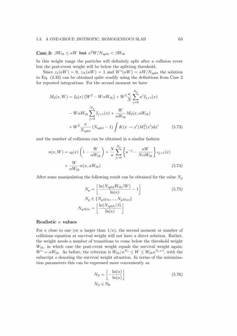
5.3. A ONE-GROUP, ISOTROPIC, HOMOGENEOUS SLAB 63
Case 3: βWth ≤ κW but κ2W/Nsplit < βWth
In this weight range the particles will definitely split after a collision eventbut the post-event weight will be below the splitting threshold.
Since z1(κW ) = 0, zN (κW ) = 1 and W ∗(κW ) = κW/Nsplit the solutionto Eq. (4.33) can be obtained quite readily using the definitions from Case 2for repeated integrations. For the second moment we have
M2(x,W ) = I0(x)(W 2 −WαWth
)+W 2 κ
N
Ng∑j=0
κjIj+1(x)
−WαWth
Ng∑j=0
Ij+1(x) +W
αWthM2(x, αWth)
+W 2 κ
Nsplit(Nsplit − 1)
∫K(x→ x′)M2
1 (x′)dx′ (5.73)
and the number of collisions can be obtained in a similar fashion
n(x,W ) = ς0(x)(
1− W
αWth
)+N
κ
Ng∑j=0
κ−j − κW
NαWth
ςj+1(x)
+W
αWthn(x, αWth) (5.74)
After some manipulation the following result can be obtained for the value Ng
Ng =⌊
ln(NsplitWth/W )ln(κ)
− 1⌋
(5.75)
Ng ∈ NgMin, ..., NgMax
NgMin =⌊
ln(Nsplit/β)ln(κ)
⌋Realistic κ values
For κ close to one (or α larger than 1/κ), the second moment or number ofcollisions equation at survival weight will not have a direct solution. Rather,the weight needs a number of transitions to come below the threshold weightWth, in which case the post-event weight equals the survival weight again;W ∗ = αWth. As before, the criterion is Wth/κ
Ns ≤ W ≤ WthκNs+1, with the
subscript s denoting the survival weight situation. In terms of the minimiza-tion parameters this can be expressed more conveniently as
NS =⌊− ln(α)
ln(κ)
⌋(5.76)
NS ∈ N0
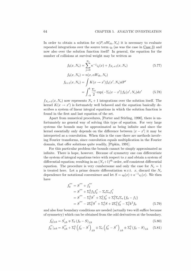
64 CHAPTER 5. ANALYTIC INVESTIGATION
In order to obtain a solution for n(P, αWth, Ns) it is necessary to evaluaterepeated integrations over the source term ς0 (as was the case in Case 3) andnow also over the solution function itself! In general, the equation for thenumber of collisions at survival weight may be written as
f0(x,Ns) =Ns∑j=0
κ−jςj(x) + fNs+1(x,Ns) (5.77)
f0(x,Ns) = n(x, αWth, Ns)
fk+1(x,Ns) =∫K(x→ x′)fk(x′, Ns)dP ′
=∫ b
−b
Σs
2exp(−Σt|x− x′|)fk(x′, Ns)dx′ (5.78)
fNs+1(x,Ns) now represents Ns + 1 integrations over the solution itself. Thekernel K(x → x′) is fortunately well behaved and the equation basically de-scribes a system of linear integral equations in which the solution function isfound in the first and last equation of the set.
Apart from numerical procedures, [Porter and Stirling, 1990], there is un-fortunately no general way of solving this type of equation. For very largesystems the bounds may be approximated as being infinite and since thekernel essentially only depends on the difference between |x − x′| it may beinterpreted as a convolution. When this is the case there are methods involv-ing Fourier transforms, since convolution equals multiplication in the Fourierdomain, that offer solutions quite readily, [Pipkin, 1991].
For this particular problem the bounds cannot be simply approximated asinfinite. There is hope, however. Because of symmetry one can differentiatethe system of integral equations twice with respect to x and obtain a system ofdifferential equation; resulting in an (Ns+1)th order, self consistent differentialequation. The procedure is very cumbersome and only the case for Ns = 1is treated here. Let a prime denote differentiation w.r.t. x, discard the Ns
dependence for notational convenience and let S = ς0(x) +κ−1ς1(x). We thenhave
f′′′′0 = S
′′′′+ f
′′′′2
= S′′′′
+ Σ2t f2f
′′2 − ΣtΣsf
′′1
= S′′′′ − Σ2
tS′′
+ Σ2t f′′0 + Σ2
tΣtΣs f0 − f1
= S′′′′ − 2Σ2
tS′′
+ Σ4tS + 2Σ2
t f′′0 − Σ2
tk2f0 (5.79)
and also four boundary conditions are needed (actually two will suffice becauseof symmetry) which can be obtained from the odd derivatives at the boundary.
f′0|±b = S
′±b ∓ Σt (f0 − S)±b (5.80)
f′′′0 |±b = S
′′′±b + Σ2
t
(f′0 − S
′)±b∓ Σt
(f′′0 − S
′′)±b± Σ3
t (f0 − S)±b (5.81)
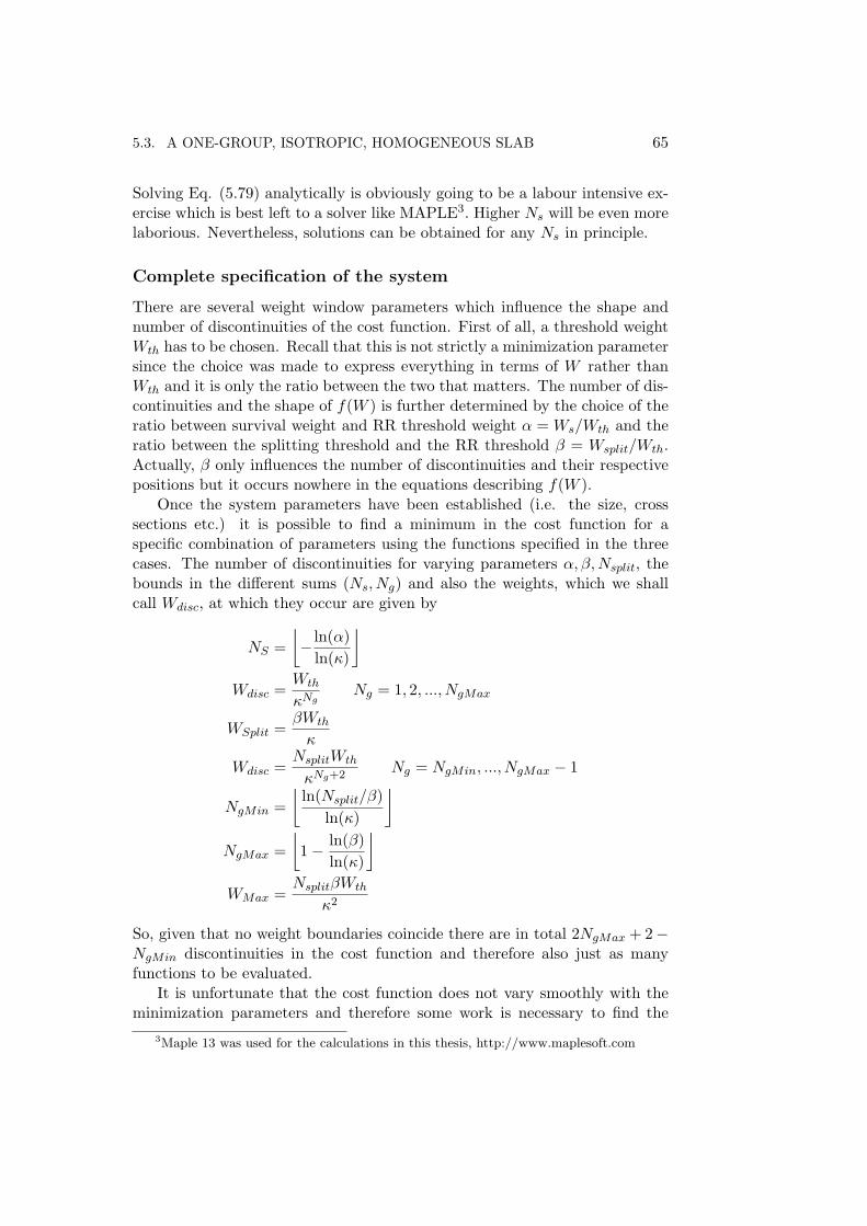
5.3. A ONE-GROUP, ISOTROPIC, HOMOGENEOUS SLAB 65
Solving Eq. (5.79) analytically is obviously going to be a labour intensive ex-ercise which is best left to a solver like MAPLE3. Higher Ns will be even morelaborious. Nevertheless, solutions can be obtained for any Ns in principle.
Complete specification of the system
There are several weight window parameters which influence the shape andnumber of discontinuities of the cost function. First of all, a threshold weightWth has to be chosen. Recall that this is not strictly a minimization parametersince the choice was made to express everything in terms of W rather thanWth and it is only the ratio between the two that matters. The number of dis-continuities and the shape of f(W ) is further determined by the choice of theratio between survival weight and RR threshold weight α = Ws/Wth and theratio between the splitting threshold and the RR threshold β = Wsplit/Wth.Actually, β only influences the number of discontinuities and their respectivepositions but it occurs nowhere in the equations describing f(W ).
Once the system parameters have been established (i.e. the size, crosssections etc.) it is possible to find a minimum in the cost function for aspecific combination of parameters using the functions specified in the threecases. The number of discontinuities for varying parameters α, β,Nsplit, thebounds in the different sums (Ns, Ng) and also the weights, which we shallcall Wdisc, at which they occur are given by
NS =⌊− ln(α)
ln(κ)
⌋Wdisc =
Wth
κNgNg = 1, 2, ..., NgMax
WSplit =βWth
κ
Wdisc =NsplitWth
κNg+2Ng = NgMin, ..., NgMax − 1
NgMin =⌊
ln(Nsplit/β)ln(κ)
⌋NgMax =
⌊1− ln(β)
ln(κ)
⌋WMax =
NsplitβWth
κ2
So, given that no weight boundaries coincide there are in total 2NgMax + 2−NgMin discontinuities in the cost function and therefore also just as manyfunctions to be evaluated.
It is unfortunate that the cost function does not vary smoothly with theminimization parameters and therefore some work is necessary to find the
3Maple 13 was used for the calculations in this thesis, http://www.maplesoft.com

66 CHAPTER 5. ANALYTIC INVESTIGATION
global minimum. However, once the solution at survival weight is found, itis simply a matter of working out the bounds and the algebraic equationsrelating the different weight range solutions to the one at survival weight.
Minimization strategy
The strategy to find the global minimum of the cost would be to first establishthe weight discontinuities and the bounds of the different sums from section5.3, given the system parameters and the minimization parameters. Subse-quently the expressions at survival weight M2(x, αWth) and n(x, αWth) needto be obtained. The functions at any weight can be expressed in terms of thesolutions at survival weight. From these functions f(W ) can be constructed byevaluating the integrals Eq. (4.35) and Eq. (4.41) and multiplying the results.This procedure needs to be repeated for a different choice of minimization pa-rameters and so forth. The global minimum of the cost may be located at adiscontinuity in W , in which case we cannot simply set the derivative of f(W )to zero and solve for W . Since many expressions need to be evaluated, thecalculations performed in this work were done with an automated algorithmwritten in MAPLE134.
Extension to source biased systems
By now the solution to the functions n(x,W ) and M2(x,W ) will be fullyknown. Trying different source biasing strategies is not an operation that willlead to fundamental complications. However, the amount of work that hasto be done to find a global minimum in the cost function will most definitelyincrease.
The way to handle this problem is to first derive the full solutionsM2(x,W )and n(x,W ) for the non-biased system and subsequently alter the initialweights according to the procedure of section 3.2, leading to M2(x,W (x))and n(x,W (x)). The integrals Eq. (4.45) and Eq. (4.48) can in principle beevaluated, but since the non-biased functions contained numerous discontinu-ities to begin with, the biased versions will contain even more. It is thereforeto be preferred to perform discrete spatial biasing; i.e. divide the source regioninto a number of uniformly biased regions.
5.4 An infinite two-group system
Another interesting system consists of a two-group, infinite system in whichup-scattering from group one to two is prohibited. As before, everything isassumed isotropic so directional dependence may be omitted straight away.The most important simplification, however, is that now also spatial depen-
4 http://www.maplesoft.com

5.4. AN INFINITE TWO-GROUP SYSTEM 67
dence can be dropped. This leads to an algebraic system of equations for themoment and number of collisions equations which can be easily solved.
Let M1g denote the first moment in group g, which is either 1 or 2 andfollow this notation for other quantities as well. The first moment equation,Eq. (4.7), then takes the following form
M11 = ηψ1 +Σ11s
Σ1t
M11 +Σ12s
Σ1t
M12
M12 = ηψ2 + κ2M12
which has solutions equal to
M12 =ηψ2
1− κ2(5.82)
M11 =ηψ1Σ1
t (1− κ2) + ηψ2Σ12s
Σ1t (1− κ2) + Σ11
s (κ2 − 1)(5.83)
The choice for a weight window makes life a bit more complicated, becausescattering from group one to group two introduces new weight range possi-bilities. Furthermore, the weight windows by no means have to be the samein the two groups. To keep matters manageable suppose the weight windowboundaries in the first group are a multiple of the window boundaries in thesecond group; i.e. Wth1 = γWth2. In practice, one would choose a fixedwindow (α, β) and let the starting weight in the respective group determinethe value of γ. A starting weight different from one may for example occurdue to source biasing, but more about that later. For the moment supposeWth2 = Wth and therefore everything is determined in terms of the windowparameters of the second group. A schematic of the weight window is givenin Fig. 5.4.
The second moment and number of collisions equation can in general bewritten as
M2g(W ) = W 2I0g + (z1(κgW ) +NzN (κgW ))κ−1g
×∑g′
Σgg′s
Σgt
M2g′(W ∗(κgW ))
+ zN (κgW )N − 1N
W 2κg∑g′
Σgg′s
Σgt
M21g (5.84)
ng(W ) = 1 + (z1(κgW ) +NzN (κgW ))κ−1g
×∑g′
Σgg′s
Σgt
ng′(W ∗(κgW )) (5.85)
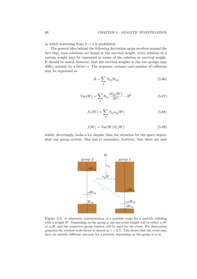
68 CHAPTER 5. ANALYTIC INVESTIGATION
in which scattering from 2→ 1 is prohibited.The general idea behind the following derivation again revolves around the
fact that, once solutions are found at the survival weight, every solution at acertain weight may be expressed in terms of the solution at survival weight.It should be noted, however, that the survival weights in the two groups maydiffer; notably by a factor γ. The response, variance and number of collisionsmay be expressed as
R =∑g
S1gM1g (5.86)
Var(W ) =∑g
S1gM2g(W )W 2
−R2 (5.87)
Nc(W ) =∑g
S1gng(W ) (5.88)
f(W ) = Var(W )Nc(W ) (5.89)
which, deceivingly, looks a lot simpler than the situation for the space depen-dent one group system. One has to remember, however, that there are now
Wth
αWth
βWth
group 2
γWth
γαWth
γβWth
group 1
γ
W
κgW
κg
Figure 5.3: A schematic representation of a possible event for a particle collidingwith a weight W . Depending on the group g, the pre-event weight will be either κ1Wor κ2W and the respective group window will be used for the event. For illustrationpurposes the window scale factor is chosen as γ = 0.5. This shows that the event mayhave an entirely different outcome for a particle, depending on the group it is in.
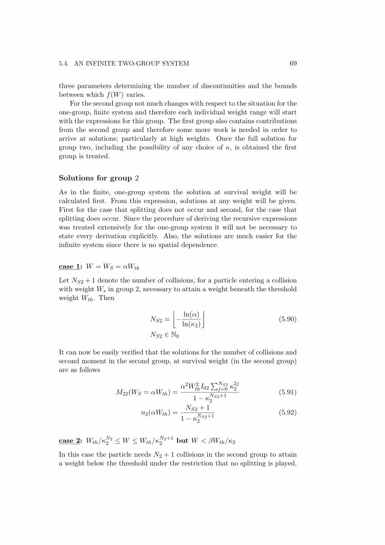
5.4. AN INFINITE TWO-GROUP SYSTEM 69
three parameters determining the number of discontinuities and the boundsbetween which f(W ) varies.
For the second group not much changes with respect to the situation for theone-group, finite system and therefore each individual weight range will startwith the expressions for this group. The first group also contains contributionsfrom the second group and therefore some more work is needed in order toarrive at solutions; particularly at high weights. Once the full solution forgroup two, including the possibility of any choice of κ, is obtained the firstgroup is treated.
Solutions for group 2
As in the finite, one-group system the solution at survival weight will becalculated first. From this expression, solutions at any weight will be given.First for the case that splitting does not occur and second, for the case thatsplitting does occur. Since the procedure of deriving the recursive expressionswas treated extensively for the one-group system it will not be necessary tostate every derivation explicitly. Also, the solutions are much easier for theinfinite system since there is no spatial dependence.
case 1: W = WS = αWth
Let NS2 + 1 denote the number of collisions, for a particle entering a collisionwith weight Ws in group 2, necessary to attain a weight beneath the thresholdweight Wth. Then
NS2 =⌊− ln(α)
ln(κ2)
⌋(5.90)
NS2 ∈ N0
It can now be easily verified that the solutions for the number of collisions andsecond moment in the second group, at survival weight (in the second group)are as follows
M22(WS = αWth) =α2W 2
thI02∑NS2
j=0 κ2j2
1− κNS2+12
(5.91)
n2(αWth) =NS2 + 1
1− κNS2+12
(5.92)
case 2: Wth/κN22 ≤W ≤Wth/κ
N2+12 but W < βWth/κ2
In this case the particle needs N2 + 1 collisions in the second group to attaina weight below the threshold under the restriction that no splitting is played.

70 CHAPTER 5. ANALYTIC INVESTIGATION
The functions of interest take the following form
M22(W ) = W 2I02
N2∑j=0
κ2j2 + κN2+1
2
W
αWthM22(αWth) (5.93)
n2(W ) = N2 + 1 + κN2+12
W
αWthn2(αWth) (5.94)
The number N2 is determined via
N2 =⌊
ln(Wth/W )ln(κ2)
⌋(5.95)
N2 ∈ 0, 1, 2, ...N2Max
N2Max =⌊
1− ln(β)ln(κ2)
⌋case 3: βWth/κ2 ≤W but W < NsplitβWth/κ
22
In this case the particle will split after experiencing its first collision. Theweight is restricted by the fact that the post-event weight should not behigher than the splitting threshold βWth. The restriction also implies thatthe post-event contribution in the equations will always be from the weightrange of case 2 under the same boundary restrictions. Therefore, the secondmoment and number of collisions can be expressed explicitly in terms of asource contribution and a contribution from the situation at survival weight
M22(W ) = W 2I02
1 +κ2
2
N
N2∑j=0
κ2j2
+ κ22W
2Nsplit − 1Nsplit
M212
+ κN2+22
W
αWthM22(αWth) (5.96)
n2(W ) = 1 +Nsplit (N2 + 1) + κN2+22
W
αWthn2(αWth) (5.97)
in which the number N2 is determined via
N2 =⌊
ln(NWth/W )ln(κ2)
− 1⌋
N2 ∈ N2Min, ..., N2Max
N2Min =⌊
ln(N/β)ln(κ2)
⌋and N2Max is as before
Now that the solutions for the entire weight range of the second group areavailable for any choice of the parameters α, β, γ,W,Nsplit, which influencethe minimization of the cost function, it is time to consider the first energygroup and its solutions for any choice of W .

5.4. AN INFINITE TWO-GROUP SYSTEM 71
Solutions for group 1
In order to establish a solution for any choice of W the first priority is to findexpressions for the situation at survival weight in the first group W = γαWth
case 1: W = γαWth
Let the number NS1 + 1 denote the number of collision, for a particle enteringits first collision in the first group, necessary to reach a weight below γWth.With this convention it is possible to write down expressions for the numberof collisions and the second moment in group one at survival weight.
M21(γαWth) = Q(γαWth)2I01
NS1∑j=0
κj1
(Σ11s
Σ1t
)j
+Q
(Σ11s
Σ1t
)NS1(
Σ12s
Σ1t
)M22(γαWth)
+Q
(Σ12s
Σ1t
)NS1∑j=1
κ−j1
(Σ11s
Σ1t
)j−1
M22(κj1γαWth) (5.98)
n1(γαWth) = Q
NS1∑j=0
κ−j1
(Σ11s
Σ1t
)j
+Q
(Σ11s
Σ1t
)NS1(
Σ12s
Σ1t
)n2(γαWth)
+Q
(Σ12s
Σ1t
)NS1∑j=1
κ−j1
(Σ11s
Σ1t
)j−1
n2(κj1γαWth) (5.99)
in which it is understood that the sums going from j = 1 should be discardedfor NS1 = 0 and
Q =
1−
(Σ11s
Σ1t
)NS1+1−1
NS1 =⌊− ln(α)
ln(κ1)
⌋(5.100)
NS1 ∈ N0
Obviously, higher values for NS1 mean more work since then more contribu-tions from the second group have to evaluated. However, once a solution isobtained one can proceed to higher weights.

72 CHAPTER 5. ANALYTIC INVESTIGATION
case 2: γWth/κN11 ≤W ≤ γWth/κ
N1+11 but W < γβWth/κ1
In this weight range it is again a matter of relating back to the case at survivalweight W = γαWth and of course, evaluating the ’in-scatter’ terms from group2. The complication arising now is that depending on the parameter γ thesecond group contribution may be from any weight for which a solution isavailable, which makes it necessary to evaluate every contribution separately.The solutions may be written as
M21(W ) = W 2I01
N1∑j=0
κj1
(Σ11s
Σ1t
)j
+W
γαWth
(Σ11s
Σ1t
)N1+1
M21(γαWth)
+W
γαWth
(Σ11s
Σ1t
)N1(
Σ12s
Σ1t
)M22(γαWth)
+(
Σ12s
Σ1t
) N1∑j=1
κ−j1
(Σ11s
Σ1t
)j−1
M22(κj1W ) (5.101)
n1(W ) =W
γαWth
(Σ11s
Σ1t
)N1+1
n1(γαWth)
+W
γαWth
(Σ11s
Σ1t
)N1(
Σ12s
Σ1t
)n2(γαWth)
+(
Σ12s
Σ1t
) N1∑j=1
κ−j1
(Σ11s
Σ1t
)j−1
n2(κj1W )
+N1∑j=1
κ−j1
(Σ11s
Σ1t
)j(5.102)
in which N1 is determined via
N1 =⌊
ln(Wth/W )ln(κ1)
⌋(5.103)
N1 ∈ 0, 1, 2, ...N1Max
N1Max =⌊
1− ln(β)ln(κ1)
⌋case 3: γαWth/κ1 ≤W but W < WMax
In this weight range splitting will occur in the first group. The restrictionimposed is, as before, that the post-event weight W ∗ should not exceed thesplitting threshold ’in the same group’. The second group contribution may

5.4. AN INFINITE TWO-GROUP SYSTEM 73
very well be in the weight range where splitting occurs. However, solutionsare only available up to a certain weight in the second group as well. Themaximum allowable weight should be smaller than some value WMax, definedby
W < WMax = Min
N2splitβWth
κ1κ22
,NsplitγβWth
κ21
(5.104)
It should further be noted that the in-group contribution will be from a weightrange below the splitting threshold and therefore it is possible to write thisterm out more explicitly.
M21(W ) = W 2I01
1 +κ1
Nsplit
(Σ11s
Σ1t
) N1∑j=0
κj1
(Σ11s
Σ1t
)j+W 2κ1
Nsplit − 1Nsplit
(Σ11s
Σ1t
)M2
11 +(
Σ12s
Σ1t
)M2
12
+
W
γαWth
(Σ11s
Σ1t
)N1+1
×(
Σ11s
Σ1t
)M21(γαWth) +
(Σ12s
Σ1t
)M22(γαWth)
+Nsplit
(Σ12s
Σ1t
) N1∑j=0
κ−(j+1)1
(Σ11s
Σ1t
)jM22(κj+1
1 W/Nsplit) (5.105)
n1(W ) = 1 +Nsplit
N1∑j=0
κ−(j+1)1
(Σ11s
Σ1t
)j+1
+W
γαWth
(Σ11s
Σ1t
)N1+1
×(
Σ11s
Σ1t
)n1(γαWth) +
(Σ12s
Σ1t
)n2(γαWth)
+Nsplit
(Σ12s
Σ1t
) N1∑j=0
κ−(j+1)1
(Σ11s
Σ1t
)jn2(κj+1
1 W/Nsplit) (5.106)
in which N1 is now determined from the post-event weight κ1W/N , from whichit follows that
N1 =⌊
ln(NWth/W )ln(κ1)
− 1⌋
(5.107)
N1 ∈ N1Min, ..., N1Max
N1Min =⌊
ln(N/β)ln(κ1)
⌋Full specification
Minimization of any of the functions with regard to the different parameterswill be quite a laborious undertaking since the functions are far from smooth

74 CHAPTER 5. ANALYTIC INVESTIGATION
and contain numerous discontinuities whose position, with respect to W , andnumber may vary with a different choice of parameters. The global minimummay be found at such a discontinuity in which case the standard tool for findinga minimum, i.e. setting the differentiated function equal to zero and solvingfor the optimal parameter choice, will yield no result. It is therefore necessaryto identify all discontinuities and the sum indexes like N1, N2 specifying thefunctions in between in a structured way.
The discontinuities arising from the in-group terms in the second groupare defined by
Wdisc =Wth
κN22
N2 = 1, 2, ..., N2max
Wdisc =βWth
κ2
Wdisc =NsplitWth
κN2+22
N2 = N2Min, ..., N2Max − 1
N2Max =⌊
1− ln(β)ln(κ2)
⌋N2Min =
⌊ln(N/β)ln(κ2)
⌋WMax =
NsplitβWth
κ22
which in total make 2N2Max + 2 − N2Min discontinuities, just as in the firstcase.
The discontinuities arising from the in-group terms in the first group aredefined by
Wdisc =γWth
κN11
N1 = 1, 2, ..., N1max
Wdisc =γβWth
κ1
Wdisc =NsplitγWth
κN1+21
N1 = N1Min, ..., N1Max − 1
N1Max =⌊
1− ln(β)ln(κ1)
⌋N1Min =
⌊ln(N/β)ln(κ1)
⌋WMax = Min
N2splitβWth
κ1κ22
,NsplitγβWth
κ21
which totals 2N1Max + 2−N1Min discontinuities.

5.4. AN INFINITE TWO-GROUP SYSTEM 75
Since the first group contains in-scatter terms from the second group whichcarry weights of κj1W and κj+1
1 W/N it is necessary to evaluate at which weightW these entry-weights will coincide with any of the 2N2Max + 2 − N2Min
discontinuities in the second group. The larger the values for N2Max, N1Max,the messier it gets obviously. For a good mathematical solver like MAPLE135
this will pose no challenge when the in-group solutions are provided.
5Maple 13 was used for the calculations in this thesis, http://www.maplesoft.com


Chapter 6
Sample cases
In the following, the equations derived in chapter 5 are applied to specificexamples. The cost function is minimized to find an optimal choice of weightwindow thresholds. Optimal source biasing is also treated in the two-groupinfinite system. All results are verified by means of Monte Carlo simulationsand the results are discussed.
6.1 A one-group, isotropic, homogeneous slab
This particular system is a good starting point for applying the theory ofchapters 4 and 5 because, although the equations are more complex than forthe case of the two group infinite system, the number of discontinuities asa function of weight is quite limited. The choice of system parameters isspecified in table 6.1. For this particular choice of parameters, the absorptionis quite high and a neutron born at x = 0 will have to traverse bΣt = 11 meanfree paths before possibly leaving the system. From this point of view, analogsimulation is unattractive. The response is the average flux over the entiresystem: ηφ = 1/V , so increasing the number of collisions, by means of implicitcapture, would seem a sensible idea as scoring can occur everywhere in the
Σt = 1.1 cm−1
Σs = 0.5 cm−1
b = 10cmκ ≈ 0.4545455k ≈ 0.8124 cm−1
Wth = 0.5
Table 6.1: A summary of system parameters for the one-group, isotropic, homoge-neous slab.
77
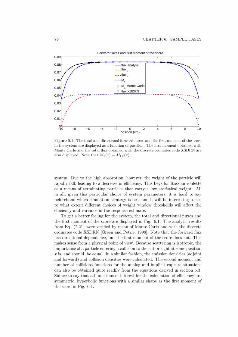
78 CHAPTER 6. SAMPLE CASES
−10 −8 −6 −4 −2 0 2 4 6 8 100
0.01
0.02
0.03
0.04
0.05
0.06
0.07
0.08
0.09
position (cm)
Forward fluxes and first moment of the score
flux analyticflux
+
flux−
M1
M1 Monte Carlo
flux XSDRN
Figure 6.1: The total and directional forward fluxes and the first moment of the scorein the system are displayed as a function of position. The first moment obtained withMonte Carlo and the total flux obtained with the discrete ordinates code XSDRN arealso displayed. Note that M1(x) = M1±(x).
system. Due to the high absorption, however, the weight of the particle willrapidly fall, leading to a decrease in efficiency. This begs for Russian rouletteas a means of terminating particles that carry a low statistical weight. Allin all, given this particular choice of system parameters, it is hard to saybeforehand which simulation strategy is best and it will be interesting to seeto what extent different choices of weight window thresholds will affect theefficiency and variance in the response estimate.
To get a better feeling for the system, the total and directional fluxes andthe first moment of the score are displayed in Fig. 6.1. The analytic resultsfrom Eq. (2.21) were verified by mean of Monte Carlo and with the discreteordinates code XSDRN [Green and Petrie, 1998]. Note that the forward fluxhas directional dependence, but the first moment of the score does not. Thismakes sense from a physical point of view. Because scattering is isotropic, theimportance of a particle entering a collision to the left or right at some positionx is, and should, be equal. In a similar fashion, the emission densities (adjointand forward) and collision densities were calculated. The second moment andnumber of collisions functions for the analog and implicit capture situationscan also be obtained quite readily from the equations derived in section 5.3.Suffice to say that all functions of interest for the calculation of efficiency aresymmetric, hyperbolic functions with a similar shape as the first moment ofthe score in Fig. 6.1.

6.1. A ONE-GROUP, ISOTROPIC, HOMOGENEOUS SLAB 79
Method R VarAnalog MC 7.745 · 10−2 ± 2 · 10−5 3.0771 · 10−3
Analog analytically 7.743322725 · 10−2 3.071512766 · 10−3
IC MC 7.74345 · 10−2 ± 6 · 10−6 3.4063 · 10−4
IC analytically 7.743322725 · 10−2 3.40052854 · 10−4
Method Nc f
Analog MC 1.7038 5.243 · 10−3
Analog analytically 1.703530999 5.232417211 · 10−3
IC MC 51.315 1.748 · 10−2
IC analytically 51.33333335 1.745604651 · 10−2
Table 6.2: Summary of the results obtained for analog simulation and a simulationcontaining only implicit capture. Results are shown obtained by analytical means andby Monte Carlo simulation. 107 particles were used for the MC results. The variancedenotes the variance in a response estimate from a single neutron history obviously.The variances in the Monte Carlo estimates of Var and Nc were not calculated.
The results for the analog and implicit capture situations are summarizedin table Table 6.2. The Monte Carlo results were obtained by simulating 107
particle histories in a simple Monte Carlo neutron transport program, writtenspecifically for this work. Var denotes the variance from a single particlehistory. The standard deviation in the response estimate is then obtained bycalculating σ =
√Var/N , in which N = 107.
From Table 6.2 it becomes clear that only implicit capture, without Rus-sian roulette as a means of terminating particles with low weight, seriouslydeteriorates the efficiency of the simulation because, although a reduction invariance of about one order of magnitude is accomplished, the number of col-lisions is increased by roughly three times that amount. This is due to the factthat a neutron history will only end if the neutron leaks out of the system.
Russian roulette and splitting
For this particular situation there are four weight window parameters of in-terest. Obviously there is W , which eventually determines an optimal choiceof the weight window lower bound or Russian roulette threshold Wth. α rep-resents the ratio of the Russian roulette threshold and the survival weightα = Ws/Wth. β represents the ratio between the splitting threshold and theRussian roulette threshold β = Wsplit/Wth. β only has influence on the num-ber of discontinuities and their locations in the range of f(W ) but not on theoverall hight of the function. Nsplit determines the number of fragments aftera splitting event
To study the effects of different choices for the weight window param-

80 CHAPTER 6. SAMPLE CASES
eters (W,α, β,Nsplit), numerous computations were performed with varyingthresholds and of course, varying initial weight W . It turns out that, forthis particular system, the parameters (α, β,Nsplit) are of marginal influencein the overall cost and/or variance reduction, albeit that a sensible choicemust be made and extreme values should be avoided. The best results wereobtained for (Wmin = 5.324, α = 2, β > 4.84, Nsplit = 2). The parameters(α = 2, β > 4.84, Nsplit = 2) should not be interpreted as the result of ’true’minimization because, for example, a value of β = 100 will result in exactly thesame minimum of f(W ). Despite the fact that the discontinuities will shift,the location at which the minimum occurs and the hight of the minimum re-mains unchanged for β > 4.84. This is due to the fact that for this system itis not favorable to implement splitting. Notice that β > Wminκ/Wth = 4.84.Shifting a little too much can obviously result in a different location and hightof the minimum. β ≤ 4.84 for example may lead to a considerable loss inefficiency. Since the above choice of weight window thresholds does lead tothe lowest possible value of f , we will simply call it the global minimum.
In the following, the result of a minimization with (α = 2, β = 9, Nsplit = 2)will be shown. From section 5.3 we can see discontinuities in the cost functionlocated at weights
Wdisc = 1.1; 2.42; 5.324; 9.9; 10.648; 23.4256;< 43.56
which means that the functions n(x,W ),M2(x,W ) are to be evaluated fora total of seven different regions. Splitting occurs from weights higher thanWsplit = βWth/κ = 9.9. The weight is bounded by the fact that a fragmentemerging from a splitting event should not split again at its next collision.
The functions n(x,W ),M2(x,W ) can be obtained by filling in the num-bers in the equations from section 5.3. The variance Var(W ) and number ofcollisions Nc(W ) can be calculated from Eq. (4.35) and Eq. (4.41), the resultsof which are depicted in Fig. 6.2.
It is clear that the theory presented in previous chapters correctly repre-sents the Monte Carlo results. The seven discontinuities are also distinctlypresent. The variance reduction flattens out quite quickly whilst the numberof collisions keeps increasing with growing W , leading to a decrease in effi-ciency. We can also clearly see a jump in the number of collision at W = 9.9,above which splitting occurs.
From the number of collisions and variance, the cost function can be con-structed through Eq. (4.44). This function, along with a detailed view aroundthe minimum and also results from Monte Carlo simulations, is depicted inFig. 6.3. The global minimum is found right at a weight discontinuity betweenthe Ng = 2 and Ng = 3 regions, Ng + 1 representing the number of collisionsnecessary to attain a weight beneath the Russian roulette threshold Wth.
We can also see that apparently it is favorable from an efficiency perspec-tive to let a particle collide three times (and no more) on average before playingRussian roulette. Splitting is not favorable as the variance barely decreases
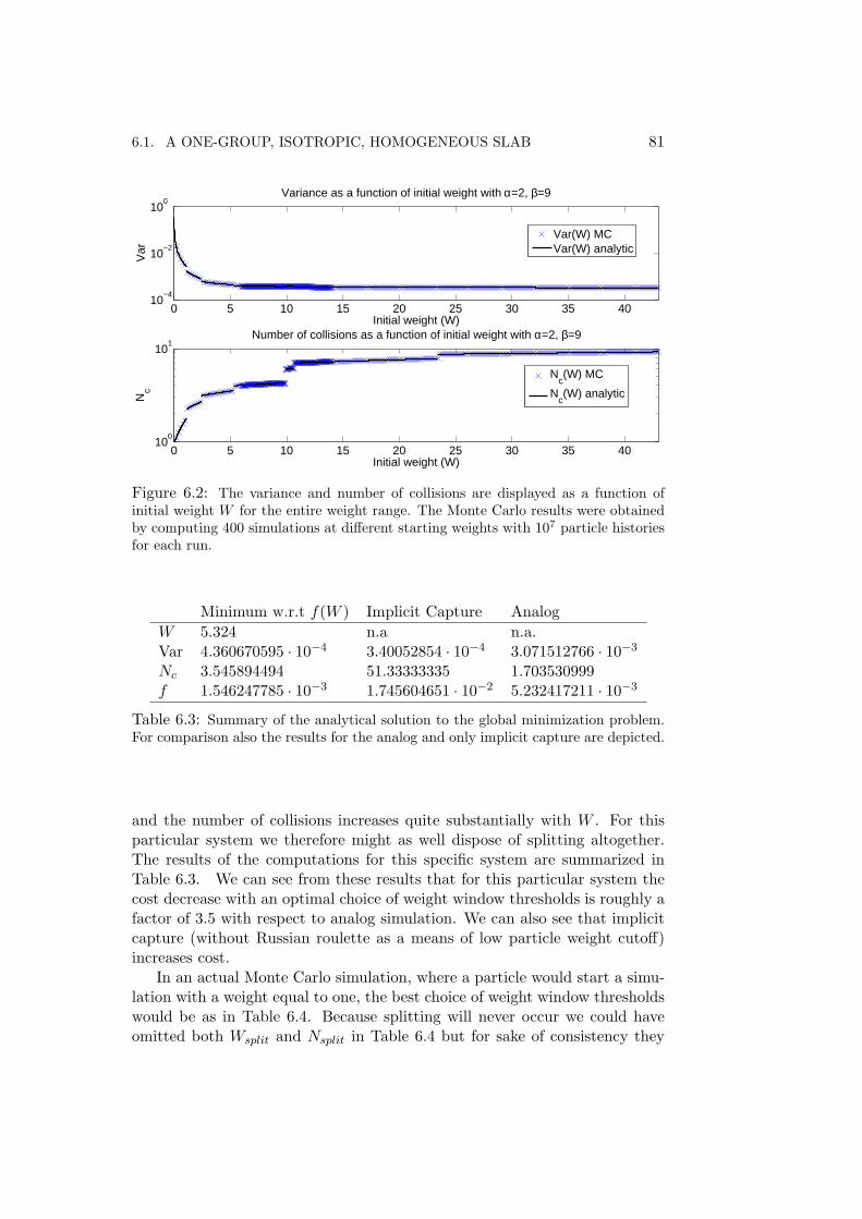
6.1. A ONE-GROUP, ISOTROPIC, HOMOGENEOUS SLAB 81
0 5 10 15 20 25 30 35 4010
−4
10−2
100
Initial weight (W)
Var
Variance as a function of initial weight with α=2, β=9
Var(W) MCVar(W) analytic
0 5 10 15 20 25 30 35 4010
0
101
Initial weight (W)
Nc
Number of collisions as a function of initial weight with α=2, β=9
Nc(W) MC
Nc(W) analytic
Figure 6.2: The variance and number of collisions are displayed as a function ofinitial weight W for the entire weight range. The Monte Carlo results were obtainedby computing 400 simulations at different starting weights with 107 particle historiesfor each run.
Minimum w.r.t f(W ) Implicit Capture AnalogW 5.324 n.a n.a.Var 4.360670595 · 10−4 3.40052854 · 10−4 3.071512766 · 10−3
Nc 3.545894494 51.33333335 1.703530999f 1.546247785 · 10−3 1.745604651 · 10−2 5.232417211 · 10−3
Table 6.3: Summary of the analytical solution to the global minimization problem.For comparison also the results for the analog and only implicit capture are depicted.
and the number of collisions increases quite substantially with W . For thisparticular system we therefore might as well dispose of splitting altogether.The results of the computations for this specific system are summarized inTable 6.3. We can see from these results that for this particular system thecost decrease with an optimal choice of weight window thresholds is roughly afactor of 3.5 with respect to analog simulation. We can also see that implicitcapture (without Russian roulette as a means of low particle weight cutoff)increases cost.
In an actual Monte Carlo simulation, where a particle would start a simu-lation with a weight equal to one, the best choice of weight window thresholdswould be as in Table 6.4. Because splitting will never occur we could haveomitted both Wsplit and Nsplit in Table 6.4 but for sake of consistency they

82 CHAPTER 6. SAMPLE CASES
0 5 10 15 20 25 30 35 4010
−3
10−2
10−1
Initial weight (W)
fCost as a function of initial weight W with α=2, β=9
f(W) MCf(W) analytic
5 5.1 5.2 5.3 5.4 5.5 5.61.54
1.56
1.58
x 10−3
Initial weight (W)
f
Cost function around optimal initial weight weight W=5.324
f(W) MCf(W) analytic
Figure 6.3: The cost function is displayed as a function of initial weight W for theentire weight range and for the range around which the minimum in the cost functioncan be found: Wmin = 5.324. The minimum occurs at the transition between theNg = 2 and Ng = 3 regions. The Monte Carlo results were obtained by computing400 simulations at different starting weights with 107 particle histories for each run.
Wth = 0.0939Ws = 0.1878Wsplit > 0.4545Nsplit = 2
Table 6.4: Weight window bounds in an actual Monte Carlo simulation, resultingfrom the minimization of f(W ) for the finite, slab system.
are retained.Further investigation would require spatial variations in weight windows,
combined with source biasing. These complications would render exact an-alytical solutions obsolete and would require numerical solutions to the mo-ment and number of collisions equations. Chapter 7 therefore deals with thederivation of equations which may be suitable for implementation in existing,deterministic neutron transport codes.
6.2 An infinite two-group system
For the infinite two-group system there are numerous variations on the systemparameters possible, but for brevity we will restrict ourselves to an interesting
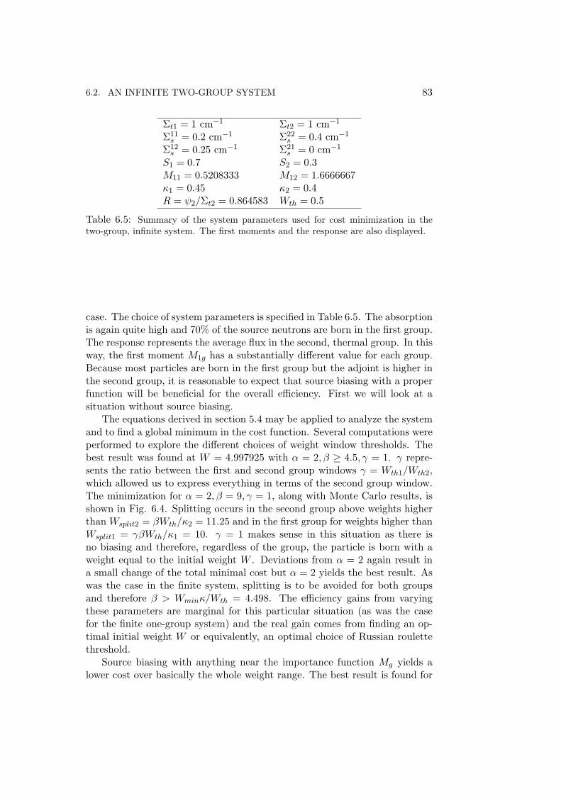
6.2. AN INFINITE TWO-GROUP SYSTEM 83
Σt1 = 1 cm−1 Σt2 = 1 cm−1
Σ11s = 0.2 cm−1 Σ22
s = 0.4 cm−1
Σ12s = 0.25 cm−1 Σ21
s = 0 cm−1
S1 = 0.7 S2 = 0.3M11 = 0.5208333 M12 = 1.6666667κ1 = 0.45 κ2 = 0.4R = ψ2/Σt2 = 0.864583 Wth = 0.5
Table 6.5: Summary of the system parameters used for cost minimization in thetwo-group, infinite system. The first moments and the response are also displayed.
case. The choice of system parameters is specified in Table 6.5. The absorptionis again quite high and 70% of the source neutrons are born in the first group.The response represents the average flux in the second, thermal group. In thisway, the first moment M1g has a substantially different value for each group.Because most particles are born in the first group but the adjoint is higher inthe second group, it is reasonable to expect that source biasing with a properfunction will be beneficial for the overall efficiency. First we will look at asituation without source biasing.
The equations derived in section 5.4 may be applied to analyze the systemand to find a global minimum in the cost function. Several computations wereperformed to explore the different choices of weight window thresholds. Thebest result was found at W = 4.997925 with α = 2, β ≥ 4.5, γ = 1. γ repre-sents the ratio between the first and second group windows γ = Wth1/Wth2,which allowed us to express everything in terms of the second group window.The minimization for α = 2, β = 9, γ = 1, along with Monte Carlo results, isshown in Fig. 6.4. Splitting occurs in the second group above weights higherthan Wsplit2 = βWth/κ2 = 11.25 and in the first group for weights higher thanWsplit1 = γβWth/κ1 = 10. γ = 1 makes sense in this situation as there isno biasing and therefore, regardless of the group, the particle is born with aweight equal to the initial weight W . Deviations from α = 2 again result ina small change of the total minimal cost but α = 2 yields the best result. Aswas the case in the finite system, splitting is to be avoided for both groupsand therefore β > Wminκ/Wth = 4.498. The efficiency gains from varyingthese parameters are marginal for this particular situation (as was the casefor the finite one-group system) and the real gain comes from finding an op-timal initial weight W or equivalently, an optimal choice of Russian roulettethreshold.
Source biasing with anything near the importance function Mg yields alower cost over basically the whole weight range. The best result is found for

84 CHAPTER 6. SAMPLE CASES
0 5 10 15 20 25 30 35 4010
0.1
100.8
Initial weight (W)
f
Cost as a function of initial weight
f(W) MCf(W) Analytical
3.8 4 4.2 4.4 4.6 4.8 5 5.2 5.41.32
1.325
1.33
1.335
Initial weight (W)
f
Cost around minimum weight W=4.5997925
f(W) MCf(W) Analytical
Figure 6.4: Results of a computation of the cost function with α = 2, β = 9, γ = 1and no source biasing. The Monte Carlo results were obtained by performing 200simulations at different weights, each with 107 particle histories.
a biasing function
Γ1 = 0.26Γ2 = 0.74
which leads, using Eq. (3.10), to a biased source distribution of
S1 = 0.4504S2 = 0.5495
This is quite close to the source distribution obtained when biasing with theimportance function, but definitely not exactly equal. For comparison, thenormalized adjoint in the second group equals M12/(M12 + M11) = 0.7619,leading to S1 = 0.4216, S2 = 0.5783. Also note that for the infinite systemthere is no distinction between the different importance functions, χ∗g = M1g.
Since, due to biasing, the initial neutron weight is modified, it is to beexpected that for optimal results γ 6= 1, because particles may be born outsidethe window in that case. From manipulation of Eq. (3.12) it follows thatan optimal value for γ should in theory, with this particular choice of biasingfunction, be γ = W 1/W 2 = 2.846 and indeed, this follows from the calculationas well. It has to be said though that, as is the case for other weight windowparameters, small deviations from this number usually do not lead to costincreases because γ determines where the discontinuities in the weight range

6.2. AN INFINITE TWO-GROUP SYSTEM 85
0 2 4 6 8 10 12 14 16 18 20
100
Initial weight (W)
f
Cost as a function of initial weight (W) with optimal biasing
9.5 10 10.5 11 11.5
0.385
0.39
0.395
Initial weight (W)
f
Cost as a function of initial weight (W) with optimal biasing
f(W) MCf(W) Analytical
f(W) MCf(W) Analytical
Figure 6.5: Minimization of the cost with α = 2, β = 9, γ = 2.8461538, using thebest biasing function. The Monte Carlo results were obtained by performing 200simulations at different weights, each with 107 particle histories.
Minimum w.r.t f(W ) Analog Non-biased BiasedW n.a. 4.5997925 10.8003422Var 2.017361 0.3712423 0.09075254Nc 1.739583 3.5684577 4.24249895f 3.509368 1.3247624 0.38501757
Table 6.6: Summary of the analytical solution to the global minimization problemfor the infinite two-group system. The results of analog, best non-biased and optimalbiased simulations are shown.
of f(W ) occur. The minimization with optimal source biasing is depicted inFig. 6.5.
Implicit capture only, without Russian roulette, obviously has no meaningin the infinite system as the variance would tend to zero and the number ofcollisions would tend to infinity. The results for the minimizations with andwithout bias, as well as analog results are shown in Table 6.6. As was the casein the one-group system, the cost decrease with respect to analog simulationin a non-biased simulation with weight windows isn’t dramatic. The costdecrease with optimal biasing this time is roughly a factor 10, which showsthat group-wise source biasing can be an effective tool for efficiency boosting.
In an actual Monte Carlo simulation with optimal biasing, the weightwindows is as in Table 6.7.

86 CHAPTER 6. SAMPLE CASES
W 2 = 0.545946 W 1 = 1.553846Wth2 = 0.046295 Wth1 = 0.13176Ws2 = 0.092589 Ws1 = 0.263523Wsplit2 = 0.416653 Wsplit1 = 1.18586
Table 6.7: Weight window bounds in an actual Monte Carlo simulation, resultingfrom the minimization of f(W ) for the infinite, two-group system. The biased, initialweights are also depicted.
Further investigation would require extending the theory to include moreenergy groups. Another possibility is to examine more complicated systemsby means of modified deterministic transport codes. Chapter 7 therefore dealswith the derivation of equations which may be suitable for implementation insuch deterministic codes.
Chapter 7
Integro-differential forms
It has been demonstrated that the theory regarding a priori calculation ofvariance and efficiency is correct and can be used to obtain an optimal choice ofweight window thresholds and biasing functions. In any realistic system thereis no hope of finding exact solutions to the variance and efficiency equationsand it is therefore necessary to be able to solve them numerically. Numericalapproximations may be attempted with Monte Carlo, employing the adjointMonte Carlo formalism of appendix B with additional modifications arisingdue to the weight dependence. This may be possible in some cases, but willlikely lead to unacceptable computing times when treating realistic systems,because the integrals that need to be solved are more complex than the actualneutron transport problem to begin with.
Another option is to try to use existing deterministic neutron transportcodes. These codes solve an integro-differential form of the neutron transportequation, Eq. (2.13). Usually they can also handle the equation adjoint toEq. (2.13). The equations that need to be solved to find an expression for theefficiency of a Monte Carlo simulation, derived in chapter 4, are not in a formthat is suitable for direct implementation in such codes and therefore someinterpretation will be necessary. To better see what the differences and simi-larities are between the equation that is solved with the existing deterministicneutron transport codes and the relevant equations from chapter 4, it is firstnecessary to transform the purely integral form to an integro-differential form.
As stated in the beginning of chapter 2, the purely integral form of neutrontransport, expressed in terms of the collision and emission density, can beobtained from the integro-differential form by applying analytic techniques[Bell and Glasstone, 1970]. The idea of the following derivations is that wewill first derive an integral equation from the integro-differential form. Oncethe solution is obtained we will follow this route backward to arrive at aresult which allows an integral equation of a particular form to be written asan integro-differential equation. Applying this result to the equations fromchapter 4 allows us to further investigate how to manipulate the existing
87
88 CHAPTER 7. INTEGRO-DIFFERENTIAL FORMS
deterministic neutron transport codes to cope with the integro-differentialform of, for example, the second moment equation or the number of collisionsequation.
The equations derived in chapter 4 contained operators with an adjointkernel K(P → P ′). As a consequence it is to be expected that the equivalentintegro-differential equation will also be of an adjoint form.
7.1 From integro-differential to integral form
Let us first state the adjoint Boltzmann equation
−Ω · ∇χ∗(P ) + Σt(r, E)χ∗(P )
=∫
4π
∫Σt(r, E)C(r, E → E′,Ω→ Ω′)χ∗(r, E′,Ω′)dE′dΩ′ + ηφ(P ) (7.1)
From Eq. (2.42) it becomes clear that the right hand side of Eq. (7.1) can berewritten to obtain
−Ω · ∇χ∗(P ) + Σt(r, E)χ∗(P ) = Σt(r, E)ψ∗(P ) (7.2)
For sake of simplicity we will assume that the total cross section is a constant.The following derivation can also be done without this simplification but thenotation will become needlessly complicated and the final result remains un-changed, [Bell and Glasstone, 1970].
Let us write r = r0 + sΩ, in which s = |r− r0| represents the path lengthbetween the two positions r and r0. Taking the derivative of χ∗ with respectto s we see that
dχ∗(r0 + sΩ)ds
=∂χ∗
∂x
dx
ds+∂χ∗
∂y
dy
ds+∂χ∗
∂z
dz
ds= Ω · ∇χ∗(r) (7.3)
We may now rewrite Eq. (7.2) as
− d
dsχ∗(r0 + sΩ, E,Ω) + Σtχ
∗(r0 + sΩ, E,Ω)
= Σtψ∗(r0 + sΩ, E,Ω) (7.4)
Multiplying Eq. (7.4) by an integrating factor exp (−Σts), we get
− d
ds
(χ∗(r0 + sΩ, E,Ω)e−Σts
)= Σte
−Σtsψ∗(r0 + sΩ, E,Ω) (7.5)
Now integrate Eq. (7.5) from 0→∞
−∫ ∞
0
d
ds
(χ∗(r + sΩ, E,Ω)e−Σts
)ds = χ∗(r, E,Ω)
=∫ ∞
0Σte−Σtsψ∗(r + sΩ, E,Ω)ds (7.6)
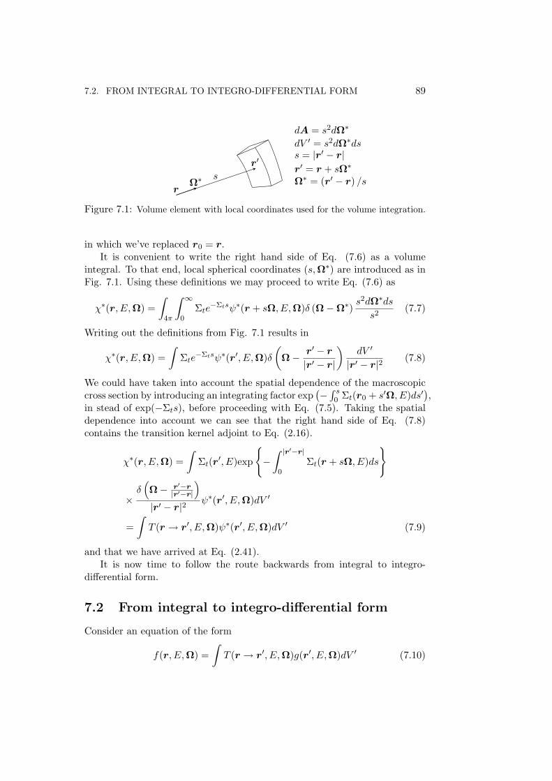
7.2. FROM INTEGRAL TO INTEGRO-DIFFERENTIAL FORM 89
r
r′
sΩ∗
dA = s2dΩ∗
dV ′ = s2dΩ∗dss = |r′ − r|r′ = r + sΩ∗
Ω∗ = (r′ − r) /s
Figure 7.1: Volume element with local coordinates used for the volume integration.
in which we’ve replaced r0 = r.It is convenient to write the right hand side of Eq. (7.6) as a volume
integral. To that end, local spherical coordinates (s,Ω∗) are introduced as inFig. 7.1. Using these definitions we may proceed to write Eq. (7.6) as
χ∗(r, E,Ω) =∫
4π
∫ ∞0
Σte−Σtsψ∗(r + sΩ, E,Ω)δ (Ω−Ω∗)
s2dΩ∗dss2
(7.7)
Writing out the definitions from Fig. 7.1 results in
χ∗(r, E,Ω) =∫
Σte−Σtsψ∗(r′, E,Ω)δ
(Ω− r′ − r
|r′ − r|
)dV ′
|r′ − r|2(7.8)
We could have taken into account the spatial dependence of the macroscopiccross section by introducing an integrating factor exp
(−∫ s
0 Σt(r0 + s′Ω, E)ds′),
in stead of exp(−Σts), before proceeding with Eq. (7.5). Taking the spatialdependence into account we can see that the right hand side of Eq. (7.8)contains the transition kernel adjoint to Eq. (2.16).
χ∗(r, E,Ω) =∫
Σt(r′, E)exp
−∫ |r′−r|
0Σt(r + sΩ, E)ds
×δ(Ω− r′−r
|r′−r|
)|r′ − r|2
ψ∗(r′, E,Ω)dV ′
=∫T (r → r′, E,Ω)ψ∗(r′, E,Ω)dV ′ (7.9)
and that we have arrived at Eq. (2.41).It is now time to follow the route backwards from integral to integro-
differential form.
7.2 From integral to integro-differential form
Consider an equation of the form
f(r, E,Ω) =∫T (r → r′, E,Ω)g(r′, E,Ω)dV ′ (7.10)

90 CHAPTER 7. INTEGRO-DIFFERENTIAL FORMS
and let us again assume, for sake of simplicity, that the total cross section isindependent of position. From Fig. 7.1, and like in Eq. (7.7) and Eq. (7.6)we can write Eq. (7.10) as
−∫ ∞
0
d
ds
f(r + sΩ, E,Ω)e−Σts
ds
=∫ ∞
0Σte−Σtsg(r + sΩ, E,Ω)ds (7.11)
As this should hold for any value of Σt ∈ [0,∞) it is reasonable to assumethat the arguments under the integral are equal for any s in the domain ofintegration and we can therefore write
− d
ds
(f(r + sΩ, E,Ω)e−Σts
)= Σte
−Σtsg(r + sΩ, E,Ω) (7.12)
from which we can see that.
−Ω · ∇f(P ) + Σt(r, E)f(P ) = Σt(r, E)g(P ) (7.13)
It is now possible to write an equation of the form Eq. (7.10) as Eq. (7.13).The interrelation between f(P ) and g(P ) then determines what the final equa-tion will look like.
The necessary boundary condition can be obtained from Eq. (7.10)
f(rb, E,Ωout) = 0 (7.14)
in which rb represents a boundary position and Ωout represents the outwarddirection at rb.
7.3 The second moment equationfor collision estimators
The second moment of the score for a particle entering a collision at P , Eq.(4.33), contains an integral over the second moment at a post-event weightand two other ’source’ terms which, for notational convenience, are writtenhere as Λ(P,W ).
Λ(P,W ) = W 2I0(P ) + zN (P, κ(P )W )W 2Nsplit − 1Nsplit
× κ(P )∫K(P → P ′)M2
1 (P ′)dP ′ (7.15)
Easing notation further by taking the event probabilities and the normaliza-tion of the kernel together to form
z(P,W ) = κ(P )−1 z1(P, κ(P )W ) +NzN (P, κ(P )W ) (7.16)

7.4. THE NUMBER OF COLLISIONS EQUATION 91
Eq. (4.33) can be written as
M2(P,W ) = Λ(P,W ) + z(P,W )∫ ∫
C(r, E → E′,Ω→ Ω′)
×Q(r, E′,Ω′,W ∗(P, κ(P )W ))dE′dΩ′ (7.17)
In this form the transition kernel is contained in the quantity Q. Notice that
Q(r, E,Ω,W ) =∫T (r → r′, E,Ω)M2(r′, E,Ω,W )dV ′ (7.18)
and note that this is exactly, asides from the weight dependence, the same formas Eq. (7.10). We can therefore proceed by stating the integro-differential formdirectly as
−Ω · ∇Q(P,W ) + Σt(r, E)Q(P,W ) = Σt(r, E)M2(P,W ) (7.19)
Using the second moment definition from Eq. (7.17) we arrive at
−Ω · ∇Q(P,W ) + Σt(r, E)Q(P,W ) = Σt(r, E)Λ(P,W )
+ Σt(r, E)z(P,W )∫ ∫
C(r, E → E′,Ω→ Ω′)
×Q(r, E′,Ω′,W ∗(P, κ(P )W ))dE′dΩ′ (7.20)
with boundary condition
Q(rb, E,Ωout,W ) = 0 (7.21)
Assuming that we are able to solve for Q(P,W ), more on that issue in section7.6, the only thing that remains is using Eq. (7.17) or Eq. (7.19) to obtainthe second moment of the score.
7.4 The number of collisions equation
For the number of collisions, Eq. (4.40), we write
n(P,W ) = ς(P ) + z(P,W )∫ ∫
C(r, E → E′,Ω→ Ω′)
× F (r, E′,Ω′,W ∗(P, κ(P )W ))dE′dΩ′ (7.22)
in which z(P,W ) is as in Eq. (7.16) and
F (P,W ) =∫T (r → r′, E,Ω)n(r′, E,Ω,W )dV ′ (7.23)

92 CHAPTER 7. INTEGRO-DIFFERENTIAL FORMS
is the form we are looking for. The full equation can therefore be written as
−Ω · ∇F (P,W ) + Σt(r, E)F (P,W ) = Σt(r, E)n(P,W )
= Σt(r, E)ς(P ) + Σt(r, E)z(P,W )∫ ∫
C(r, E → E′,Ω→ Ω′)
× F (r, E′,Ω′,W ∗(P, κ(P )W ))dE′dΩ′ (7.24)
with boundary condition
F (rb, E,Ωout,W ) = 0 (7.25)
Once F (P,W ) is obtained, n(P,W ) is calculated from Eq. (7.24).
7.5 Track-length estimators
The most commonly used estimator in practice will be a track-length esti-mator. It is therefore necessary to treat the integro-differential form of thesecond moment equation for the track-length estimator here. Recall that forthe derivation we looked at a neutron starting a flight rather than a neutronentering a collision. This meant that, from Fig. 4.3, there was first a transitionfrom r to r′. Recall Pe = (r′, E,Ω) and write Eq. (4.53) as follows
M2tl(P,W ) =∫T (P → Pe)Stl(Pe)dV ′ +
∫T (P → Pe)z(Pe,W )
×∫ ∫
C(Pe → P ′)M2tl(P ′,W ∗(Pe, κ(Pe)W ))dE′dΩ′dV ′ (7.26)
from which the integro-differential form can immediately be obtained.
−Ω · ∇M2tl(P,W ) + Σt(r, E)M2tl(P,W ) = Σt(r, E)Stl(P,W )
+ Σt(r, E)z(P,W )∫ ∫
C(r, E → E′,Ω→ Ω′)
×M2tl(r, E′,Ω′,W ∗(P, κ(P )W ))dE′dΩ′ (7.27)
The boundary condition is
M2tl(rb, E,Ωout,W ) = 0 (7.28)
We see that the different interpretation of the adjoint kernels K(P → P ′)and L(P → P ′) leads to a different interpretation of the equivalent integro-differential equations for the respective second moments. The result of (7.27)is actually more appealing than Eq. (7.20) as it is in closed form already;solving the equation immediately returns the second moment. The integralform, Eq. (4.53) was most definitely less appealing than Eq. (4.33).

7.6. PRACTICAL IMPLEMENTATION 93
For the number of collisions equation, Eq. (4.56), derived for a particlestarting a flight we can write the following
−Ω · ∇ntl(P,W ) + Σt(r, E)ntl(P,W ) = Σt(r, E)ς(P )
+ Σt(r, E)z(P,W )∫ ∫
C(r, E → E′,Ω→ Ω′)
× ntl(r, E′,Ω′,W ∗(P, κ(P )W ))dE′dΩ′ (7.29)
with boundary condition
ntl(rb, E,Ωout,W ) = 0 (7.30)
7.6 Practical implementation
There are several complications one faces when trying to obtain Var(W ) andNc(W ) by means of an algorithm, based on the possibility of solving themoment and number of collision equations at a certain weight with an existingdeterministic neutron transport code.
First there is the choice which equations are the best starting point. Whilethe integral forms of the second moment equation and the number of collisionsequations for a particle entering a collision were more appealing than theintegral forms of the equations for a particle starting a flight, it is the otherway around for the integro-differential form. Asides from this fact there is thepossibility to treat both collision estimators and track-length estimators withEq. (7.27), given a proper choice of the scoring function ηψ(P, Pe). This isnot the case for Eq. (7.20) because it can only handle collision estimators.
Now suppose the second moment and number of collisions are available ata certain weight. It is still a matter of evaluating the weighted integrals, forexample Nc(W ) =
∫S1(P )n(P,W )dP , to obtain the variance and number of
collisions at a certain weight. Evaluating integrals containing the source offirst collisions is less appealing from a practical point of view as the physicalsource will be available and the source of first collisions has to be calculated.
Calculating the source of first collisions can obviously be done by meansof a deterministic code. The integro-differential form follows from the resultsobtained in previous sections quite readily
Ω · ∇S1(P ) + Σt(r, E)S1(P ) = Σt(r, E)S(P ) (7.31)
with boundary condition
S1(rb, E,Ωin) = 0 (7.32)
Comparing Eq. (7.31) with Eq. (2.13) we see that, in order to obtain asolution, the correct source has to be given as input and scattering has to beput to zero.

94 CHAPTER 7. INTEGRO-DIFFERENTIAL FORMS
The real difficulty lies in how to handle the weight dependence and howto handle the modified collision probabilities. Deterministic codes solve anequation of the form Eq. (7.1). The source is not an issue as it can simplybe specified for any weight. The collision kernel, however, has to be modifiedaccording to
C(r, E → E′,Ω→ Ω′,W ) = z(P,W )C(r, E → E′,Ω→ Ω′) (7.33)
In existing deterministic neutron transport codes like PARTISN [Alcouffe andBaker, 2005], XSDRN [Green and Petrie, 1998], and DALTON [van Rooijenand Lathouwers, 2007], energy dependence is treated in energy groups g anddiscrete angles Ωm are used to treat angular dependence. Under the assump-tion that only a scattering event produces neutrons at the new energy anddirection we can write the collision kernel as
C(r, E → E′,Ω→ Ω′) =Σgg′s (r)
Σgs(r)
p(Ωm ·Ωm′ |g → g′) (7.34)
in which p(Ωm · Ωm′ |g → g′) represents the probability to have a change indirection from Ωm to Ωm′ given a change in energy from group g to g′. Thescalar product stems from the fact that scattering usually only depends onthe scattering angle cosine Ωm ·Ωm′
Somehow we have to incorporate z(P,W ) in the group-scatter cross sec-tions. Strictly, z(P,W ) may still depend on direction, but we will drop thisdependence as it will rarely be encountered in practice. We write a modifiedgroup scatter cross section as
Σgg′s (r,W ) = z(r, g,W )Σgg′
s (r)
=Σgt (r)
Σgs(r)
z1(r, g, κ(r, g)W ) +NzN (r, g, κ(r, g)W )Σgg′s (r) (7.35)
The event-probabilities zN (r, g, κ(r, g)W ) and z0(r, g, κ(r, g)W ) need to becalculated for a certain weight and possibly as a function of position. Thecross section library has to be modified subsequently to arrive at a propercollision kernel.Suppose this all works out, we can for example write Eq. (7.27) as
−Ωm · ∇ntl(r, g,Ωm,W ) + Σt(r, g)ntl(r, g,Ωm,W ) = ς(r, g,Ωm)
+∑g′
∑m′
Σt(r, g)C(r, g → g′,Ωm → Ωm′ ,W )ntl(r, g′,Ωm′ ,W∗) (7.36)
in which W ∗ = W ∗ (r, g,Ωm, κ(r, g)W ) and ς(r, g,Ωm) = Σt(r, g)ς(r, g,Ωm).Despite Eq. (7.36) having the correct form to be solved by means of a
deterministic code, the issue of the pre- and post-event weights not beingequal remains.

7.6. PRACTICAL IMPLEMENTATION 95
At this point suppose that there is a constant weight window (in bothenergy and space), a constant κ and that always κ(P )Ws ≤Wth. Under theserestrictions Eq. (7.36) at survival weight, or any of the above equations forthat matter, can be written in the following form
−Ωm · ∇ntl(r, g,Ωm,Ws) + Σt(r, g)ntl(r, g,Ωm,Ws) = ς(r, g,Ωm)
+∑g′
∑m′
Σt(r, g)C(r, g → g′,Ωm → Ωm′ ,Ws)
× ntl(r, g′,Ωm′ ,Ws) (7.37)
with boundary condition
ntl(rb, g,Ωm,out) = 0 (7.38)
This equation is self consistent, in the correct form and can therefore besolved by means of a deterministic code. Once the solution of this equation isobtained, solutions at any weight can in principle be obtained by going fromvery low, approaching zero, weights to progressively higher weights. This isdue to the fact that the post-event weight W ∗ will always be equal to thesurvival weight or lower than the pre-event weight, in which case the solutionis available. Obviously also the equations for the only implicit capture andanalog situations can be solved as there is no weight dependence present inthat case.
Omitting the restrictions regarding the energy and spatial dependence ofboth weight window and non-absorption probability and also that κ(P )Ws Wth, will seriously complicate matters. We will not try to give an answerhere as to how these complications can be overcome. In chapter 5 a greatdeal of effort went into solving issues like these. For general applicationsone would need to devise a smart, automated algorithm to handle the weightdependence.


Chapter 8
Discussion and Conclusions
8.1 Discussion
In chapter 4 the cost as a function of initial weight f(W ), a multiplicationof expected variance and number of collisions resulting from a single neutronhistory, was introduced as a workable alternative to the Figure Of Merit.The necessary moment and number of collisions equations were derived froma probability score distribution, which proved to be a powerful and versatileconcept. Despite the fact that the most commonly used non-analog simulationtechniques were treated in this work, there are numerous other non-analogtechniques possible, all of which would require their own derivation of momentand number of collisions equations. The formalism presented in chapter 4should now make these derivations possible in most cases.
The derivations presented in chapter 4 were, however, concerned with fixedsource problems. Dealing with a fission source, in which case the neutrontransport equation becomes an eigenvalue equation for the effective multipli-cation factor keff , will require some extensions of the theory in order to arriveat an expression for the cost/efficiency of a simulation.
In practice, an initial fission source distribution is guessed, and after anumber of cycles this distribution converges to the correct distribution, [Sjen-itzer, 2009]. Collisions of neutrons may lead to fission events which generatethe source for the next cycle. Despite this difference, once the correct eigen-function is obtained we essentially still have a fixed source problem to whichthe formalism presented in chapter 4 is applicable. As an approximation thefission source may, for example, be calculated with an existing deterministicneutron transport code and used as input. The generation of offspring willnot likely lead to complications1 in the derivation of moment and number ofcollisions equations.
Exact analytic solutions to the variance and efficiency equations are dif-
1A splitting event may actually be considered as the production of offspring during acollision, which allows the concepts from section 4.3 to be used for the treatment of fission.
97

98 CHAPTER 8. DISCUSSION AND CONCLUSIONS
ficult, if not impossible, to obtain for any realistic simulation. Nevertheless,exact solutions to equations describing the efficiency of a Monte Carlo simula-tion in which the response is obtained with a collision estimator were found inchapter 5 for the simplified two-directional transport model. Most work wentinto solving issues arising from the fact that the equations contained differentpre- and post-event weights. The expressions derived in 5 were put to the testin chapter 6. Numerous analytic computations were performed, all of whichmatched the results from Monte Carlo simulations perfectly, giving full con-fidence that the theory derived in chapter 4 is correct. The global minimumof the cost function was established at a particular choice of weight windowthresholds.
From the investigation it followed that setting the weight window lowerbound (the Russian roulette threshold weight Wth) has the largest effect onthe overall cost/efficiency. The choice of survival weight and weight windowupper bound (the splitting threshold Wsplit) have a marginal influence on thetotal cost. These parameters largely determine the discontinuities in the costfunction but do not lead to a dramatic increase/decrease in cost.
It was shown that in some cases splitting is to be avoided from an efficiencyperspective, leading to a lower bound for β (the ratio of the splitting andRussian roulette threshold). The default value in the general purpose MonteCarlo code MCNP for β is 5, which is quite close to the lower bound found forboth the one-group finite system and the two-group infinite system. This posesthe question if β = 5 will generally be best. α = 2, the ratio of the survivalweight threshold to the Russian roulette threshold, showed the best resultsconsistently. From the simple systems studied in this work it is impossibleto infer generalizations regarding the choice of parameters like α and β. Itdoes show that an optimal choice can, and should, be given for each particularsimulation and that the tools presented in this work allow to find an optimalchoice in principle.
For a two-group infinite system, section 5.4 and 6.2, exact expressionswere also obtained. The weight window was allowed to vary per group, whichrequired extra effort to treat all the subtleties arising from the weight depen-dence of the equations. From a large number of computations it was shownthat the analytic results agreed fully with results from Monte Carlo simula-tions and that in this case also an optimal choice of weight window thresholdscan be obtained by minimizing the cost function.
Source biasing computations were also performed, which interestingly showedthat biasing the source distribution with the adjoint flux is not necessarily thebest option. Further investigation is required because in practice, biasing thesource with the adjoint is an accepted strategy and it may turn out that thisis not optimal.
If source biasing is implemented, the initial neutron weight becomes afunction of phase space as well. The group wise effects have been studied andshowed that it is best to choose the group weight window such that the neutron

8.2. CONCLUSIONS 99
should neither split nor play Russian roulette immediately at its first collision.This is a confirmation of what is accepted in practice. Further investigationis of course needed, especially of the spatial dependence.
Chapters 5 and 6 showed that in order to be able to use the theory inpractice, numerical approximations to the variance and efficiency equationswill be a necessity since analytic solutions are hard to come by.
The integro-differential forms derived in chapter 7 showed a number ofinteresting things. The moment and number of collisions equations for a track-length estimator (derived for neutrons starting a flight) have an appealingintegro-differential form, whereas the integral form was rather unappealing.This observation is encouraging since track-length estimators are used mostfrequently in practice. As a side note, a proper choice of scoring functionallows these expressions to be used for a collision estimator as well. It isnot hard to incorporate the modified collision probabilities, now a function ofweight, into a modified collision kernel. The efficiency of analog simulationsand simulations containing only implicit capture can be obtained with onlymodest modifications.
The complications arising from the difference in pre- and post-event weights,however, remain. In chapters 5 and 6 some examples were given as to how todeal with these problems but the possibility of dealing with spatially varyingweight windows, common in practice, was not treated. An algorithm needsto be devised to deal with this issue for the theory to be applied in a generalcontext. Once such an algorithm exists, cost minimization can be employedto quickly initiate a particular simulation in an optimal way, general ’rulesof thumb’ like biasing the source with the adjoint flux and accepting defaultparameters like β = 5 can be studied. Essentially, the efficiency of practi-cally all neutron transport Monte Carlo simulations would benefit from thedevelopment of such an algorithm.
8.2 Conclusions
• It is possible to obtain expressions for the a priori calculation of varianceand efficiency of a neutron transport Monte Carlo simulation for a varietyof non-analog simulation strategies.
• The formalism in which moment and number of collision equations arederived from a probability score distribution allows for easy extensionto other simulation strategies and possibly to Monte Carlo applicationsin other fields as well.
• It is best to start the derivation of the cost function at a neutron enteringa collision when using a collision estimator and at a neutron starting aflight when using a track-length estimator.

100 CHAPTER 8. DISCUSSION AND CONCLUSIONS
• Exact analytical expressions for the efficiency can be obtained for simplesystems. Any realistic system will render this possibility obsolete.
• The cost function can be used for the a priori optimization of weight win-dow thresholds and for finding optimal source biasing functions. Numer-ical results from actual Monte Carlo simulations show exact agreementwith the analytical results obtained in this work.
• For the practical implementation of the theory presented in this workit will be necessary to devise an algorithm to cope with the weight de-pendence in the integro-differential form of the moment and number ofcollisions equations.
• Although it is impossible to infer generalizations from the two systemsstudied in this work, it has been shown that one needs to tread care-fully when accepting general rules of thumb like biasing with a specificimportance function or using default weight window thresholds, as it isquestionable if these rules of thumb will be best in a particular situation.
• The theory of cost minimization to optimize neutron transport MonteCarlo simulation strategies a priori shows great potential and, if fu-ture developments lead to a quick and automated algorithm to perform(approximated) cost minimization, may significantly increase computa-tional efficiency.

Bibliography
R. E. Alcouffe and R. S. Baker. Partisn: A time-dependent, parallel neutral particletransport code system. Technical Report LA-UR-05-3925, Los Alamos NationalLaboratory, 2005. [cited at p. 94]
G. I. Bell and S. Glasstone. Nuclear Reactor Theory. van Nostrand Reinhold, 1970.[cited at p. 10, 12, 87, 88]
J. G. Christiano. Differentiation of the repeated integral. The American MathematicalMonthly, 66(2):127–129, 1959. [cited at p. 52]
R. R. Coveyou and K. J. Yost V. R. Cain. Adjoint and importance in monte carloapplication. Nuclear Science and Engineering, 27:219–234, 1967. [cited at p. 30]
J. J. Dunderstadt and L. J. Hamilton. Nuclear Reactor Analysis. John Wiley andsons, 1976. [cited at p. 3, 9, 10]
N. M. Green and L. M. Petrie. Xsdrnpm: A one-dimensional discrete ordinates codefor transport analysis. NUREG/CR-0200 ORNL/NUREG/CSD-2/V2/R6, OakRidge National Laboratory, 1998. [cited at p. 78, 94]
A. Haghighat and J. C. Wagner. Monte carlo variance reduction with deterministicimportance functions. Progress in nuclear energy, 42(1):25–53, 2003. [cited at p. 27]
J. E. Hoogenboom. Adjoint Monte Carlo Methods in Neutron Transport Calculations.Delft University Press, 1977. [cited at p. 13, 19, 107]
J. E. Hoogenboom. Theoretical and practical study of the variance and efficiencyof a monte carlo calculation due to russian roulette. Physor, 160:1–22, 2004.[cited at p. 29]
J. E. Hoogenboom. The two-direction neutral particle transport model: a useful toolfor research and education. Transport theory and statistical physics, 37:65–108,2008. [cited at p. 48]
Los Alamos National Laboratories. Mcnp5 a general monte carlo n-particle transportcode, version 5. Technical report, University of California, 2008. [cited at p. 27]
I. Lux and L. Koblinger. Monte Carlo Particle Transport Methods: Neutron andPhoton Calculations. CRC Press, 1991. [cited at p. 12, 19, 23, 24, 29, 30, 103]
101

102 BIBLIOGRAPHY
P. K. MacKeown. Stochastic Simulation in Physics. Springer Verlag, 1997.[cited at p. 5]
C. A. Laury Micoulaut. The nth centred moment of a multiple convolution and itsapplications in an intercloud gas model. Astronomy and Astrophysics, 51:343–346,1976. [cited at p. 37, 38]
A. C. Pipkin. A course on integral equations. Springer Verslag, 1991. [cited at p. 14,
20, 64]
D. Porter and D. S. G. Stirling. Integral Equations. Cambridge university press, 1990.[cited at p. 64]
Y. Ronen. CRC Handbook of Nuclear Reactors Calculations, volume 3. CRC PressInc., 1986. [cited at p. 15]
Stochastic signal analysis. Nuclear Reactor Analysis. John Wiley and sons, 1976.[cited at p. 103]
B. Sjenitzer. Variance reduction using the correcton method on criticality calculations.Master’s thesis, Delft, University of technology, 2009. [cited at p. 97]
J. Spanier and E. M. Gelbard. Monte Carlo Principles and Neutron Transport Prob-lems. Addison-Wesley, 1969. [cited at p. 19]
J. M. Thijssen. Computational Physics. Cambridge University Press, 2007.[cited at p. 6]
W.F.G. van Rooijen and D. Lathouwers. Sensitivity analysis of the kinetic behaviourof a gas cooled fast reactor to variations of the delayed neutron parameters. In MCconference Monterey USA, 2007. [cited at p. 94]
F. Vermolen, J. van Kan, and A. Segal. Numerical Methods in Scientific Computing.VSSD, 2008. [cited at p. 3]

Appendix A
Statistics and estimation
Some basic concepts from statistics and some notation used throughout thiswork require introduction here. The notation is based on [Lux and Koblinger,1991] and for a more extensive treatment the reader is advised to consult[signal analysis, 1976].
A random variable represents the set of possible outcomes of some randomevent, like throwing dice (discrete), or the size of a solar flare (continuous).The probabilities associated with these outcomes are characterized by theprobability mass function pmf (discrete) or probability density function pdf(continuous). Furthermore, any function of a random variable will itself be arandom variable.
Suppose that we consider a random variable S with associated pdf π(s).The expected value of the process E[S] = 〈S〉π, or in light of applications inchapter 4, the first moment M1, of this random variable is given by
E[S] =∫sπ(s)ds = M1 (A.1)
for the continuous case. The integral runs over the ensemble of possible out-comes s and π(s)ds represents the probability to get an outcome of s in ds.For the discrete case obviously
M1 =∑i
siπ(si) (A.2)
The expected value or first moment represents the average outcome of therandom event, described by the random variable S.
A measure for how much the outcomes of the random event will deviatefrom the average is given by the variance Var(S).
Var(S) = E[S − E[S]2] = E[S2]− E[S]2 = M2 −M21 (A.3)
with the second moment M2 = E[S2]. Most outcomes of the random eventare expected to be within one standard deviation σ(S) =
√Var(S) from the
expected value.
103

104 APPENDIX A. STATISTICS AND ESTIMATION
The expectation value and variance or standard deviation are usuallyenough to characterize the random event. It is possible to extend the the-ory to higher moments, but this is irrelevant for the purposes of this work.
Suppose now that we only have N independent random observations si ofthe random event and we want to know the expected value and the variance.We can estimate E[S] with the sample mean estimator S
S =1N
N∑i=1
si ≈ E[S] (A.4)
in which the approximate sign may be dropped as (N → ∞), a result betterknown as the law of large numbers. This estimate is called unbiased;
Bias(S) = E[S]− E[S] = 0 (A.5)
since it delivers the expectation value on average.The variance may be estimated from the limited number of samples as
well. An unbiased estimate of the variance is given by
Var(S) =1
N − 1
N∑i=1
(si − S
)2=
1N − 1
N∑i=1
s2i −
1N
(N∑i=1
si
)2 (A.6)
The devision by (N − 1) may be understood as loosing one degree of freedomto the calculation of S.
The variance in the sample mean estimator is given by
Var(S) =1
N(N − 1)
N∑i=1
s2i −
1N
(N∑i=1
si
)2 =
Var(S)N
(A.7)
which shows that the variance in the mean scales with the number of samples.This is another way of expressing the law of large numbers since, given enoughsamples (N → ∞) the variance in the sample mean will tend to zero andtherefore the sample mean, if unbiased, will tend to the true mean.

Appendix B
Adjoint Monte Carlo
In particular situations, adjoint Monte Carlo may be much better suited toestimate a response. The source and payoff functions are interchanged. There-fore, problems in which the payoff function is nonzero in a small region of phasespace and the source is distributed over a large region in phase space, can inprinciple much better be treated by adjoint Monte Carlo.
The adjoint equations Eq. (2.34) and Eq. (2.36) can in principle be solvedby means of Monte Carlo, but there are some complications arising from theadjoint interpretation of the transport kernels. The adjoint transport kernelin the form of a transposition of the forward kernel, L(P → P ′), is not wellsuited for MC implementation. Rather, we need an adjoint kernel of the formL∗(P ′ → P ), or more explicitly; we are looking for a transformation such thatwe can play the adjoint game like a forward Monte Carlo game. The derivationthat follows can also be done starting from the kernel K(P → P ′), but sincethe adjoint equations are so closely related this is more or less irrelevant forthe final result.
As stated we are looking for a relation such that the adjoint Monte Carlogame can be played in a similar fashion as is the case in forward calculations.For the adjoint kernel L we demand the following relation
L(P → P ′) ≡ T (r → r′, E,Ω)C(r′, E → E′,Ω→ Ω′)L∗(P ′ → P ) = T ∗(r′ → r, E,Ω)C∗(r′, E′ → E,Ω′ → Ω) (B.1)
Next we will see that it is possible to show an equivalence between the trans-posed transition kernel and the desired transition kernel. Recall Eq. (2.16)and divide by the total cross section. After some manipulation and using the
105

106 APPENDIX B. ADJOINT MONTE CARLO
substitution s′ = |r − r′| − s we see
T (r → r′, E,Ω)Σt(r′, E)
= exp−∫ |r′−r|
0Σt(r′ − sΩ, E)ds
δ(Ω− r′−r|r−r′|)
|r − r′|2
= exp−∫ |r−r′|
0Σt(r + s′Ω, E)ds′
δ(Ω′ + r−r′
|r−r′|)
|r − r′|2
=T (r′ → r, E,−Ω)
Σt(r, E)(B.2)
From which we can obtain a reasonable choice for the adjoint transition kernel,suited for Monte Carlo sampling
T ∗(r′ → r, E,Ω) = T (r′ → r, E,−Ω) (B.3)
This is a ’normal’ kernel, subject to the same normalization conditions as theregular transition kernel. Given this particular choice for the adjoint transitionkernel we can see that apparently the adjoint ’particles’ move in the directionopposite to their direction vector. Also from Eq. (B.2) the definition of theadjoint collision kernel can be obtained
C∗(r′, E′ → E,Ω′ → Ω) =Σt(r′, E)Σt(r, E)
C(r′, E → E′,Ω→ Ω′) (B.4)
Note that this kernel is generally not normalized. Together with the definitionof the collision kernel from Eq. (2.17) we now arrive at a transport kernelwhich, subjected to the right normalization conditions, can be sampled forMC purposes by first sampling the adjoint collision kernel for (E,Ω) andafterwards selecting a new collision site r from the adjoint transition kernel.
L∗(P ′ → P ) =T (r′ → r, E,−Ω)Σt(r′, E)
Σt(r, E)C∗(r′, E′ → E,Ω′ → Ω)
=T (r′ → r, E,−Ω)
Σt(r, E)
×∑A
∑j
Σj|A(r′, E)cj|A(E)pj|A(E → E′,Ω→ Ω) (B.5)
Although Eq. (B.5) might not seem as a direct improvement, it can beput to good use when the following transformation is made
χ(P ) = Σt(r, E)χ∗(P ) (B.6)
ψ(P ) = Σt(r, E)ψ∗(P ) (B.7)
This transformation makes sense from a physical point of view as well sincethe new function ψ(P ), for example, will behave more like an event density,

107
in stead of a flux like quantity which is less suited for Monte Carlo implemen-tation. We also see the factor Σt(r, E) in the denominator of Eq. (B.5).
The transformed equation for the transformed adjoint quantity, with re-spect to Eq. (2.36), can be written as
χ(P ) = fχ(P ) +∫L∗(P ′ → P )χ(P ′)dP ′ (B.8)
in which
fχ(P ) = Σt(r, E)ηχ(P ) (B.9)
The transformed kernel is written as
L∗(P ′ → P ) =Σt(r, E)Σt(r′, E′)
L∗(P ′ → P ) = T (r′ → r, E,−Ω)
×∑A
∑j
Σj|A(r′, E)Σt(r′, E′)
cj|A(E)pj|A(E → E′,Ω→ Ω′) (B.10)
The only thing missing now is proper normalization of collision part of thekernel. The normalization factor is given by
N∗(P ′) =
∫ ∫ ∑A
∑j Σj|A(r′, E)cj|A(E)fj|A(E → E′,Ω→ Ω′)dEdΩ
Σt(r′, E′)
=Σ∗(r′, E)Σt(r′, E)
(B.11)
The new quantity Σ∗ appearing in Eq. (B.11) is called the adjoint crosssection. It has some rather special characteristics which go beyond the scopeof this thesis. A full treatment of the adjoint cross section can be found inHoogenboom [1977]. Adjoint simulation can now be done by selecting (E,Ω)from the normalized ’adjoint’ collision kernel
C∗N (r′, E′ → E,Ω′ → Ω) =∑A
∑j
Σj|A(r′, E)Σ∗(r′, E)
cj,A(E)pj,A(E → E′,Ω→ Ω′) (B.12)
and selecting new collision sites from the transition kernelT (r′ → r, E,−Ω). From Eq. (2.39) we see that fχ(P ) acts as a source of firstcollisions
fχ(P ) =∫fψ(r′, E,Ω)T ∗(r′ → r, E,Ω)dV ′ (B.13)

108 APPENDIX B. ADJOINT MONTE CARLO
in which fψ(P ) = Σt(P )ηψ(P ). From Eq. (2.41) and Eq. (2.42) we can deducethe following pair of equations for the transformed adjoint densities
ψ(P ) = fψ(P )
+∫N∗(r, E′)C∗N (r, E′ → E,Ω′ → Ω)χ(r, E′,Ω′)dE′dΩ′ (B.14)
χ(P ) =∫T (r′ → r, E,−Ω)ψ(r′, E,Ω)dV ′ (B.15)
For completeness and to see the striking resemblance with the forwardsituation, Eq. (2.21) and Eq. (2.24), let us express the transformed quantitiesin terms of themselves at other points in phase space by manipulating theequation pair, Eq. (B.14).
ψ(P ) = fψ(P ) +∫T (r′ → r, E′,−Ω′)
×N∗(r, E′)C∗N (r, E′ → E,Ω′ → Ω)ψ(r′, E′,Ω′)dP ′ (B.16)
χ(P ) = fχ(P ) +∫N∗(r′, E′)C∗N (r′, E′ → E,Ω′ → Ω)
× T (r′ → r, E,−Ω)χ(r′, E,Ω)dV ′ (B.17)
from which we can see that ψ takes on the role of the forward emission densityχ and χ takes on the role of the forward collision density ψ.
The response can be expressed in terms of the transformed densities asfollows
R =∫S(P )
χ(P )Σt(P )
dP =∫S1(P )
ψ(P )Σt(P )
dP (B.18)
Now that we’ve seen how to treat transport the only thing that remainsis the source density. Other than the fact that fψ need not be normalizedthis should given no complications. One can sample the normalized pdffψ(P )/
∫fψ(P )dP and simply multiply the final result by
∫fψ(P )dP .
The series expansion solution of the type two Fredholm integral equationpair, Equations (B.14) is the following
ψ0(P ) = fψ(P ) (B.19)
χ0(P ) =∫T (r′ → r, E,−Ω)ψ0(r′, E,Ω)dV ′ (B.20)
i+ 1 = 1, 2, ...,∞
ψi+1(P ) =∫N∗(r, E′)C∗N (r, E′ → E,Ω′ → Ω)χi(r, E′,Ω′)dE′dΩ′ (B.21)
χ(P )i+1 =∫T (r′ → r, E,−Ω)ψi+1(r′, E,Ω)dV ′ (B.22)
which directly leads to the Monte Carlo procedure for adjoint transport, de-picted in Table B.1.

109
Do for N ’particles’ from j = 1...Nset i = 0 and proceed until leakage or absorption
1: Sample fψ(P )/∫fψ(P )dP for initial coordinates (r0, E0,Ω0)
2: Possibly score at an emission3: Sample T (ri → ri+1, Ei,−Ω)i for next collision site ri+1
4: Possibly score at a collision5: Multiply weight by N∗(ri+1, Ei)6: Sample C∗N (ri+1, Ei → Ei+1,Ωi → Ωi+1) for (Ei+1,Ωi+1)
Set Pi = (ri+1, Ei+1,Ωi+1) and return to 2:Determine Rj from the score collected during history jand proceed with the next history
Table B.1: Monte Carlo procedure for adjoint, non-analog transport.


Appendix C
Coefficients
Let I0(x) = A0 +A1 cosh(kx) with
A0 = η2φ
2k2− 1
Σ2t
A1 = −η2
φ
2k2
Σs
k sinh(kb) + Σt cosh(kb)
and let
l =√
Σ2t − Σ2
s
From which the coefficients can be expressed more easily as
Ca0 =Σ2t
k2A0
Ca2 = −ΣtΣs
2kA1
Ca1 =Σt (A0 − Ca0) + sinh(kb) (kA1 − ΣtbCa2 − Ca2) + cosh(kb) (ΣtA1 − bkCa2)
k sinh(kb) + Σt cosh(kb)
Ci0 =Σ2t
l2A0
Ci2 = − Σs
k2 − l2A1
Ci1 =Σt (A0 − Ci0) + sinh(kb)kA1 − sinh(lb)lCi2 + cosh(kb)ΣtA1 − cosh(lb)ΣtCi2
k sinh(kb) + Σt cosh(kb)CM0 = Ca0
CM2 = Ca2
CM1 = Ca1
111

A PRIORI EFFICIENCY CALCULATIONSFOR MONTE CARLO APPLICATIONS
IN NEUTRON TRANSPORTPNR-131-2008-009Andreas van Wijk
Delft, January 6, 2010