a prediction of individual growth of height according …. inst. statist. math. vol. 43, no. 4,...

Ann. Inst. Statist. Math. Vol. 43, No. 4, 607-619 (1991)

A PREDICTION OF INDIVIDUAL GROWTH OF HEIGHT ACCORDING TO AN EMPIRICAL BAYESIAN APPROACH*

TAKAO SHOHOJI ], KOUJI KANEFUJI 2 **, TAKAHIRO SUMIYA 1 AND TAO QIN 2

1 Faculty of Integrated Arts and Sciences, Hiroshima University, Hiroshima 730, Japan

2 Graduate School of Engineering, Hiroshima University, Higashihiroshima 724, Japan

(Received February 27, 1990; revised April 12, 1991)

A b s t r a c t . An empirical Bayesian approach is applied to a prediction of an individual growth in height at an early stage of life. The sample has 548 normal growth of Japanese girls whose measurements are available on request. The prior distribution of estimator of the growth parameter vector in a lifetime growth model is obtained conventionally from the least squares estimates of the growth parameters. The choice of prior distributions is discussed from a practical point of view. It is possible to obtain a relevant prediction of growth based upon only measurements during the first six years of life. The lifetime prediction of individual growth at the age of 6 is enough approximation of real measurements obtained. This report deals with the comparison between the least squares estimates and an empirical Bayes estimates of the growth parameters and the characteristic points of the growth curve. We discuss the mean-constant growth curves of the groups classified by the height intervals at the age of 6.

Key words and phrases: Empirical Bayes prediction, fundamental growth model, growth model, height, individual growth, mean-constant growth curve, non-linear regression, prediction, stature.

1. Introduction

Many statist ical growth studies have focused on growth model building and growth model comparison. Many physical growth models of human height have been proposed since Jenss and Bayley (1937) dealt with a well f i t ted nonlinear growth model of height for children up to six years. Count (1943) a t t empts at describing a lifetime growth model of height. Preece and Baines (1978) deal with four

* This work was supported in part by the ISM Cooperative Research Program (2-ISM.CRP- 63).

** Now at The Institute of Statistical Mathematics, 4-6-7 Minami-Azabu, Minato-ku, Tokyo 106, Japan.

607

608 TAKAO SHOHOJI ET AL.

asymptotic lifetime growth models of height. Based upon a fundamental growth model, Shohoji and Sasaki (1987) discuss the Count-Gompertz type growth curve as an asymptotic individual lifetime growth from infancy to adulthood. Jolicoeur et al. (1988) propose a new type of seven-parameter growth models of height from the day of fertilization to adulthood.

Rao (1975) has proposed an empirical Bayesian approach for a linear growth model. Bock and Thissen (1980) discuss a Bayes estimation of individual growth when data are incomplete. For the least squares estimation of growth parameters, Berkey (1982) applies an empirical Bayesian approach to the estimation of growth parameters in growth model during childhood. Shohoji et al. (1987) apply an empirical Bayesian approach to an individual and an average lifetime growth curve based upon the Count-Gompertz type growth model.

When we predict an individual lifetime growth in height at an early age of life, we may not have enough information to predict a lifetime growth in height. Thus, we cannot use a regular type of least squares method or of maximum likelihood method to estimate and to characterize an individual lifetime growth. We may apply an empirical Bayesian approach to a prediction of an asymptotic individual lifetime growth at an early age of life. The mean and the variance-covariance matrix of the prior distribution of growth parameters may be conventionally regarded as the sample mean and the sample variance-covariance matrix of the estimates of growth parameters, respectively. Thus, we can make an asymptotic lifetime growth predicted by effectively using the information on growth parameters of the proper population that she belongs to.

2. Materials

The sample is a part of the Hiroshima Growth Study sample that has 548 Japanese girls growing up normally. Almost all were born between 1965 and 1968. Most of the girls aged between 6 and 18, were measured once a year. The age intervals between any successive measurements are at most five years for each girl who has her measurement at birth. The measurements until about the age of 18 have been retrospectively collected. These reliable data are collected from an official pocket book for the mother and baby in Japan, the records of school health cares and so on. These records may be available on request to the editorial office of this Journal.

Table 1 shows the fundamental statistics of the height at the time of examination and the menarcheal age. One year is 365 days through out this report. Some girls have been measured more than once during a yearly age interval. Eleven out of 548 Japanese girls have no information on their menarcheal ages. The method of iteration for estimating the growth parameters does not converge for two girls ($93152 and $96150). We obtain the least squares estimates of the growth parameters for 546 girls. The number of samples, that the difference between the estimate of the growth parameter U in the growth model and the maximum height obtained is larger than 3 cm, is 86 out of 546 girls. Conventionally, an empirical Bayesian approach does not deal with these unsuitably fitted 86 girls. Finally, we use only 460 girls for this growth analysis.

P R E D I C T I O N OF INDIVIDUAL G R O W T H 609

Table 1. The fundamenta l s ta t is t ics of height by age intervals and menarcheal age.

Age at S t anda rd measurement Size Mean deviat ion Min imum Maximum

(Years)

Height (cm)

At b i r t h 548 49.72 2.16 39.5 57.0

0 968 63.81 6.29 48.0 80.4

1 299 76.40 4.45 67.0 93.4

2 148 87.43 4,67 75.0 100.0

3 420 94.75 4.28 84.5 109.8

4 217 102.31 4.79 90.9 114.6

5 244 107.90 4.82 93.5 120.2

6 585 113.70 4.65 101.9 126.0

7 527 119.86 5.05 106.6 134.5

8 529 125.70 5.50 108.5 145.0

9 529 131.72 6.26 114.6 154.2

10 530 138.41 7.07 117.7 160.3

11 534 144.90 7.09 122.4 163.1

12 523 149.87 6.15 t30.8 165.0

13 527 153.41 5.31 138.7 167.7

14 527 155.27 5.03 140.2 169.4

15 540 156.08 5.00 141.0 172.1

16 525 156.67 4.86 142.0 172.1

17 530 156.89 4.92 142.0 172.1

18 272 157.04 4.96 140.8 172.1

Age at menarche (in months)

537 148.7 14.1 74.3 197.3

Note: Some girls are measured more t h a n once dur ing a yearly age interval and some others are not measured.

For getting an empirical Bayes estimate of asymptotic lifetime growth based upon the individual measurements obtained, at least six measurements are necessary until the age at prediction. Eleven out of 460 girls have no information on their menarcheal ages. Two girls do not have enough number of measurements until their menarcheal ages to obtain the empirical Bayes estimates at menarche.

The empirical Bayes estimates of lifetime growth for 191 out of 460 girls are obtained from the data until the age of 6 (72 months old). The 269 girls do not have enough numbers of measurements to get their empirical Bayes estimates at the age of 6. Thus, 191 girls are the essential sample for discussing an empirical Bayesian approach of growth prediction at the age of 6.


3. Growth model

It is strongly desirable that any mathematical growth models can describe some biological phenomenon of growth from a biological point of view. The model selection in growth study should not be considered only from a view point of goodness of fit because every growth model is asymptotic after all. For example, the growth parameters and some properties of the growth model universally interpret biological and physical meanings as much as possible. It is desirable that the estimates of growth parameters and characteristic points of growth curve should be stable from a viewpoint of numerical calculation.

Let Yt be the height (cm) at age t (month). A growth model of height from birth to adult is

Yt = H(t; O) + et

where 0 is a growth parameter vector, et is a random error and H(t; O) is a distance curve. Many authors (Preece and Baines (1978), Berkey (1982)) have made such an assumption that the errors are uncorrelated for an observation scheme being welt spread out in time.

Shohoji and Sasaki (1985) introduce a fundamental lifetime growth model as

H(t; O) = g(t; 8) + J(t; O)[U - H(t; O)]

for the growth of weight in savannah baboon. Here, we apply the fundamental growth model to the growth in human height. Now, we consider that the parameter U is the young adult height, g(t; O) is a growth curve of height during infancy and childhood, and J(t; O) is a relative amount of measure of maturi ty at age t from a viewpoint of growth in height. Many functional forms are available for g(t;0) and J(t;O). Shohoji and Sasaki (1987) deal with the Count model g(t; ~) = C + D t + E log t as a growth curve of height during infancy and childhood. We cannot use the measurement at birth for this model. But the measurements at birth play important role for characterizing an individual growth. Sasaki et al. (1987) introduce a modified Count model g(t; O) = C + Dt + Elog(t + 1) so that the measurement at birth can be used for estimating the growth parameters. On the other hand, a relative amount of measure of maturity during adolescence J(t; 0), is considered as an S-shaped Gompertz function. This function is almost all zero before the adolescent growth spurt. The following model is induced from the fundamental growth model.

The distance curve H(t) and its velocity curve h(t) at age t are, respectively, defined as

~ _ - - - - U - - e A - B t H(t) [C + Dt + Elog(1 + t)](1 e eA--Bt) -~ and

h(t) = ( 1 - e - ~ - ~ ) D + i-- ~

if- B e A - B t - e A - B t [ g - C - Dt - E log(1 + t)]

where A, B, C, D, E and U are the elements of six-dimensional individual growth parameter vector O. This velocity curve has empirically single local maximum

PREDICTION OF INDIVIDUAL GROWTH 611

180

160-

140 -

E 12o -

C ::Z

. . l O 0 - ,.c:

80-

6 0 -

40

0

Japanese Girl (S16205) /~;::"

.-z~" :'" Measurements used " ~ ~ . f o ~ estimat iosi~ii~S

.,'/ ~ All

'., old

........ " <9 years old

f X AMS:::jsm:::ments " f " ' ~ __

. . . . . A,ze in month (t) . . . . i "s" "P'J ~ ' "q" I . . . .

60 120

O

E --1.0 "~

--0.8 .=

- 0 . 6 o 0 > e -

- -0 .4

- 0 . 2

0.0 180 240

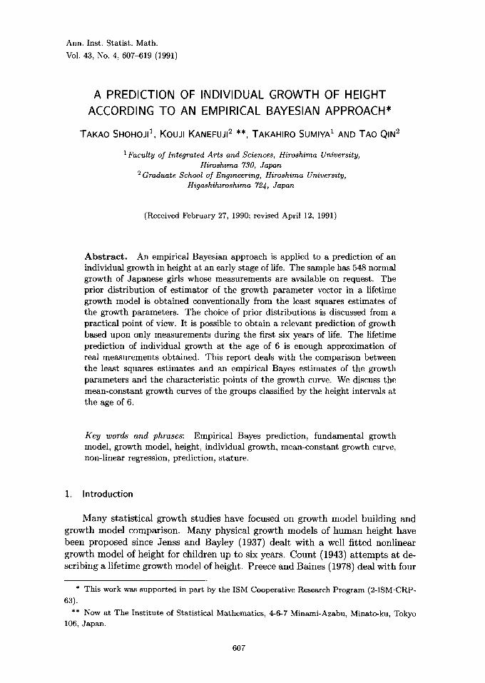
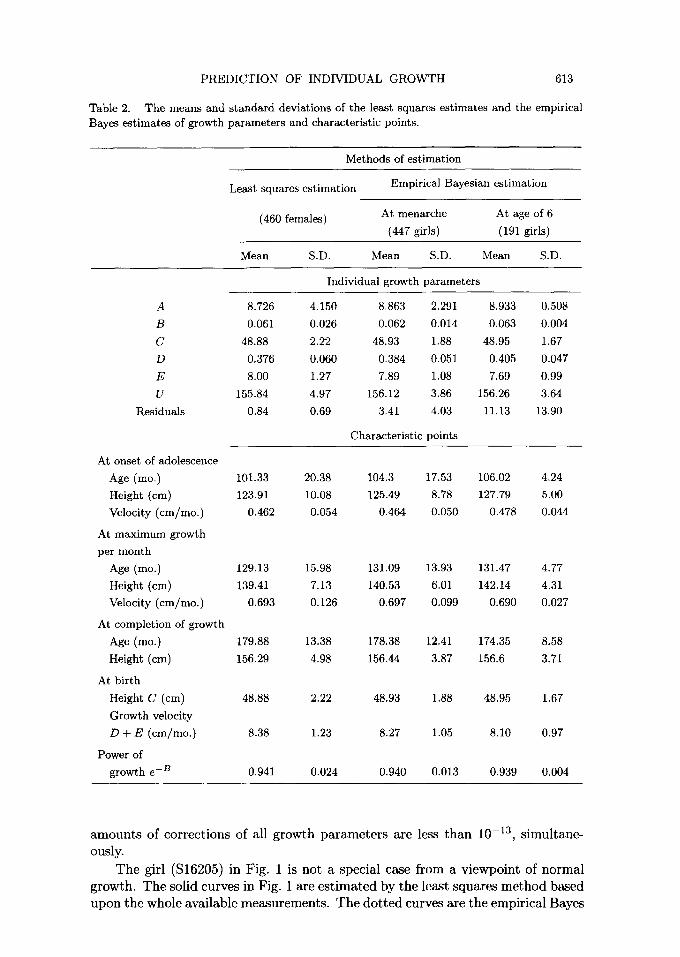
Fig. 1. The least squares estimates of an individual growth curve and its two empirical Bayes estimates. The solid curves are the least squares estimates of the growth curve. One dotted curves are predicted from the measurements obtained until the age of 6. The other dotted curves are predicted from the measurements until the age of 9.

and two local minimums such that one local minimum is positive and the other is negative.

The solid curves in Fig. 1 present a graphical representation of the proposed growth model fitted to a set of measurements (S16205 in the Hiroshima Growth Study sample). The scales of distance curve H(t) and its velocity curve h(t) are, respectively, plotted on the left and the right hand side vertical axes. Many characteristic points of the growth curve can be mathematically defined. The points M, S, P and Q on the age axis are the ages at characteristic points of the growth curve. The point M is the age at menarche. The age at onset of adolescence (age at take-off point, say, onset age) S is the younger age attaining the local minimums of the velocity curve. The age at maximum growth P is the age attaining the local maximum during adolescence. The age at completion Q is conventionally defined as the age attaining the five percent value of the local maximum of the velocity curve during adolescence. From a feature of the growth model, the final adult height slightly decreases after attaining the maximum height. Thus, Table 2 shows that there exists a little difference between the mean of estimates of U and the mean of heights estimated at the age at completion.

The value e - s is an index of individual growth power during adolescence. The values of C and D + E are the height and the growth velocity at birth, respectively. D may be recognized as an underlying growth velocity during infancy and childhood.

Kanefuji and Shohoji (1990) deal with the growth model comparison among the Preece-Baines model (1978), the Jolicoeur et al. model (1988) and the proposed model, and with the comparison of the goodness of fit among these models for 365


Japanese girls. The goodness of fit of the last two models is almost same and the proposed model is a little better than the Jolicoeur et aL model from an AIC point of view.

4. Empirical Bayesian approach

If we predict an individual lifetime growth at an earliest possible age, we must have enough number of measurements to predict an individual lifetime growth. There is such a big problem that these data do not contain any measurements after the age at prediction. But an empirical Bayesian approach overcomes the issues by making an efficient use of the sample mean and the sample variance- covariance matrix of growth parameters obtained from the suitable population. The prior distribution of growth parameters may be obtained from a set of the least squares estimates of individual growth parameters. A growth model is established to fit sufficiently and there exists sufficient number of data to estimate them. An empirical Bayesian approach can predict an asymptotic individual lifetime growth.

We apply the method of scoring to the least squares estimation of individual growth parameters. The initial trial values for the iteration is automatically set up from the measurements obtained such that

(1) the initial trial values of U and C are the final height and the height at birth, respectively,

(2) to get the initial trial values of the growth parameters D and E, the linear regression is applied only to the measurements until the rough onset age of her adolescence, and

(3) to obtain the initial trial values of A and B, the transformation w~ -- log{- log{[Yt - g ( t ; ~ ) ] / [ U - g(t; 8)]}} is used and the linear regression of A and B is applied to the new variable wt. The criterion of convergence for this iteration is that the relative amount of correc- tion for every unknown parameter is simultaneously less than 0.001. The method of scoring does not converge when the number of iteration is greater than 200.

In predicting a growth, the measurements obtained until the age of prediction are utilized for estimating and predicting an asymptotic lifetime growth curve. For getting an empirical Bayes estimates of growth parameter vector 0 (Berkey (1982)), we minimize the value

without any restrictions on the growth parameters where n is the number of available measurements, y is an n-dimensional measurement vector and ge(Y) is the ex- pectation of y. The sample estimates of # and E for the prior distribution N(#, E) are obtained from the least squares estimates of individual growth parameters.

When the Newton-Raphson method is applied to the minimization of A with respect to 0, the equations become complicated. Here, we apply Zangwill (1967) to simplification of a computer program for the empirical Bayesian approach. The sample mean of the growth parameter vector 0 is used as an initial trial value of ~ for minimizing A. The criterion of convergence for this iteration is that the


Table 2. The means and standard deviations of the least squares estimates and the empirical Bayes estimates of growth parameters and characteristic points.

Methods of estimation

Least squares estimation

(460 females)

Empirical Bayesian estimation

At menarche At age of 6

(447 girls) (191 girls)

Mean S.D, Mean S.D. Mean S.D.

Individual growth parameters

A 8.726 4.150 8.863 2.291 8.933 0.508

B 0.061 0.026 0.062 0.014 0.063 0.004

C 48.88 2.22 48.93 1.88 48.95 1.67

D 0.376 0.060 0.384 0.051 0.405 0.047

E 8.00 1.27 7.89 1.08 7.69 0.99

U 155.84 4.97 156.12 3.86 156.26 3.64

Residuals 0.84 0.69 3,41 4.03 11.13 13.90

Characteristic points

At onset of adolescence

Age (mo.) 101.33 20.38 104.3 17.53 106.02 4.24

Height (cm) 123.91 10.08 125.49 8.78 127.79 5.00

Velocity (cm/mo,) 0,462 0.054 0.464 0.050 0.478 0.044

At maximum growth

per month

Age (mo.) 129.13 15.98 131.09 13.93 131.47 4.77

Height (cm) 139,41 7.13 140,53 6.01 142.14 4.31

Velocity (cm/mo.) 0.693 0.126 0.697 0.099 0.690 0.027

At completion of growth

Age (mo.) 179.88 13.38 178.38 12.41 174.35 8.58

Height (cm) 156.29 4.98 156.44 3.87 156.6 3.71

At birth

Height C (cm) 48.88 2.22 48.93 1.88 48.95 1.67

Growth velocity

D + E (cm/mo.) 8.38 1.23 8.27 1.05 8.10 0.97

Power of

growth e - B 0.941 0.024 0.940 0.013 0.939 0.004

a m o u n t s of c o r r e c t i o n s of al l g r o w t h p a r a m e t e r s a r e less t h a n 10 -13 , s i m u l t a n e -

ously.

T h e gir l (S16205) in F ig . 1 is no t a spe c i a l case f rom a v i e w p o i n t of n o r m a l

g rowth . T h e so l id cu rves in F ig . 1 a r e e s t i m a t e d by t h e l eas t s q u a r e s m e t h o d b a s e d

u p o n t h e w h o l e a v a i l a b l e m e a s u r e m e n t s . T h e d o t t e d curves a r e t h e e m p i r i c a l Bayes


estimates based upon the measurements obtained until about the age of 6 or 9. It should be mentioned that no measurements on and after the age of 6 are available for predicting a lifetime growth in height at the age of 6. Figure 1 presents the comparison among three estimates of the growth curve when we use the prior distribution obtained from the least squares estimates of growth parameters.

Only measurements until the menarche are used for obtaining the empirical Bayes estimates at menarche. Other empirical Bayes estimates are obtained from the available measurements in the first six years of life. For convenience, the mean and the variance-covariance matrix of prior distribution are obtained from the ordinary least squares estimates for all individuals. Table 2 presents the sample means and standard deviations of the least squares estimates and two empirical Bayes estimates for an individual growth. The empirical Bayes estimates at menarche are closer to their ordinary least squares estimates based upon whole available measurements than their empirical Bayes estimates at the age of 6.

To get better empirical Bayes estimates, we have to choose more suitable prior distribution of growth parameters for a target individual, because there are many types of growth patterns according to the living environments and the genetic factors.

5. Selection of prior distribution

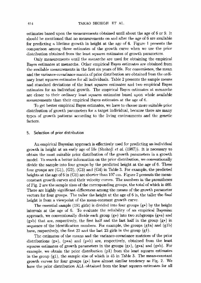
An empirical Bayesian approach is effectively used for predicting an individual growth in height at an early age of life (Shohoji et al. (1987)). It is necessary to obtain the most suitable prior distribution of the growth parameters in a growth model. To search a better information on the prior distribution, we conventionally divide the sample into four groups by the predicted height at the age of 6. These four groups are (G1), (G2), (C3) and (G4) in Table 3. For example, the predicted heights at the age of 6 in (G1) are shorter than 107 cm. Figure 2 presents the mean- constant growth curves and their velocity curves. The numbers in the parentheses of Fig. 2 are the sample sizes of the corresponding groups, the total of which is 460. There are highly significant differences among the means of the growth parameter vectors for four groups. The taller the height at the age of 6 is, the taller the final height is from a viewpoint of the mean-constant growth curve.

The essential sample (191 girls) is divided into four groups (g*) by the height intervals at the age of 6. To evaluate the reliability of an empirical Bayesian approach, we conventionally divide each group (g,) into two subgroups (g,a) and (g,b) that are, respectively, the first half and the last half in the group (g,) in sequence of the identification numbers. For example, the groups (gla) and (glb) have, respectively, the first 22 and the last 23 girls in the group (gl).

The estimates of the means and the variance-covariance matrices of the prior distributions (p*), (p,a) and (p,b) are, respectively, obtained from the least squares estimates of growth parameters in the groups (g,), (g,a) and (g,b). For example, we obtain the prior distribution (pl) from the least squares estimates in the group (gl), the sample size of which is 45 in Table 3. The mean-constant growth curves for four groups (g,) have almost similar tendency as Fig. 2. We have the prior distribution ALL obtained from the least squares estimates for all


Table 3. The mean of mean squares of residuals of empirical Bayes estimation.

Heights at age 6 (cm)

< 107 10~110 110-113 113+

Groups (G1) (G2) (G3) (G4) Sizes 100 119 125 116

The samples who have not enough number of measurements to predict the growth at the age of 6

Sizes 55 78 72 64

The samples who can predict the lifetime growth at age 6

Groups (gl) (g2) (g3) (g4) Sizes 45 41 53 52

Empirical Bayes estimates at age of 6

(pl): < 107 12.44(16.96) 10,00(10.95) 17.19(13.87) 50.63(58.68) (p2): 107-110 21.40(20.30) 6.65(6.37) 15.02(11.06) 64.01(44.11) (p3): 110-113 46.21(33.98) 15.30(10.45) 7.64(7.75) 22.24(26.55) (p4): 113+ 32.14(31.62) 19.87(18.44) 15.01(17.22) 8.86(6.68) ALL 13.94(19.44) 10.59(13.80) 11.37(13.17) 8.55(6.96)

Least squares estimates (191 girls)

0.85(0.47) 0.95(0.55) 1.00(0.84) 1.05(0.66)

Note: The numerical values in the parentheses 0 are standard deviation.

191 girls. From Fig. 2, there are at least four types of growth pa t te rns in height of Japanese girls. Thus, the most proper prior dis tr ibut ion should be chosen at predict ing an asymptot ic lifetime growth of a target individual.

Table 3 summarizes the means and the s tandard deviations of mean square of residuals for the least squares est imates and the empirical Bayes estimates based upon various prior distr ibutions of growth parameters . The row of the prior dis- t r ibut ion (p*) in Table 3 presents the results tha t the prior (p , ) is applied to all four groups (g*) for predict ing their lifetime growth at the age of 6. For example, we apply the prior dis t r ibut ion (p l ) to 45 girls of the group (gl) . The mean of their mean squares of residuals is 12.44 and their s tandard deviat ion is 16.96. The 55 girls in the group (G1) have not enough number of measurements to predict their growth at the age of 6. At applying the prior distr ibution (p2) to the group (gl) , the mean of mean square of residuals is 21.40. The last row in Table 3 gives the mean of mean square of residuals for the ordinary least squares est imates of 191 girls, for whom we obta in the empirical Bayes est imates at the age of 6.

The best prior dis t r ibut ion is individually different because the growth has a great influence from the living environments and the genetic factors. It is im-


180

160

140 E

12o

80

60

40

/~', . / / . ,/(o~) {,,. . 1 " / * z

..z'J:"

((33) . . . . . . . . . (125) 110 - 1]3 (134) .. . . . . . . . (116) 113 +

A~e in Month (0 . . . . I . . . . I . . . . I

60 120 180

O Lo E

- 0 . 8

- - 0.6 .~ O O

--0.4 >" -E

--0.2 o

- - 0.0

-0.2

Fig. 2. The mean-constant growth curves divided by the height intervals at the age of 6. The numbers in the parentheses 0 are the sample sizes.

Table 4. Comparison of mean of mean squares of residuals of two empirical Bayes estimation for two different prior distributions.

Prior distributions

Groups Sizes (p.a) (p,b)

Empirical Bayes estimates at age 6

< 107 (gl) 45

g l a 22 14.29(18.45) 15.68(22.25)

g l b 23 10.03(7.76) 10.12(10.19)

107-110 (g2) 41

g2a 20 7.95(9.62) 9.10(7.34)

g2b 21 7.17(5.39) 4.83(2.90)

110-113 (g3) 53

g3a 26 8.61(8.01) 8.14(7.48)

g3b 27 7.44(7.86) 6.77(7.92)

113+ (g4) 52

g4a 26 7.96(5.77) 8.02(5.94)

g4b 26 11.78(9.00) 8.85(6.82)

Note: The numerical values in the parentheses 0 are standard deviation, g*a and g*b are,

respectivery, the first half and the last half of the group g* in the sequance of identification

numbers. The prior distributions, p*a and p .b , are obtained from the groups, g*a and g.b,

respectivery.


portant to choose a better prior distribution at applying an empirical Bayesian approach to an actual individual. The mean of mean square of residuals, being bold faced in Table 3, is the smallest value among the four empirical Bayes estimates (within the column) for each group. The best prior distribution for each group is the prior distribution obtained from the corresponding group. For example, the best prior distribution for the group (gl) is the prior distribution (pl). When a lifetime growth is predicted at the age of 6, we had better use the prior distribution of the group to which a target individual at the age of 6 belongs. But the best prior distribution of an empirical Bayes estimation for the groups (g4) is the prior obtained from the whole effective sample.

Table 4 presents sixteen means of mean square of residuals for eight subgroups to each of which we apply two corresponding prior distributions. In predicting a lifetime growth at the age of 6, we get two corresponding means of mean squares of residuals. These means are almost all the same, whether a target individual belongs to a subgroup used for obtaining the prior distribution or not. This verifi- cation gives an evaluation of the reliability of the empirical Bayes estimation, that is proposed for predicting an individual growth curve.

5. Discussion

An individual growth curve is more useful and more practical than an average or a median growth curve of population from a clinical point of view. The clinical interest is obvious to obtain a proper prediction of an individual future growth. It should be emphasized at practical and statistical analysis based upon individual growth, that only one measurement is available at each time of observation for any individual. That is, we cannot get any repeated measurements at each time of examination for any individual. Even if an observation scheme is well designed from a statistical point of view, the age interval between successive measurements is not always equal from a viewpoint of practical data collection for a human growth study. But, it is well known that the estimators of individual growth parameters are consistent and asymptotically normally distributed under certain regularity conditions.

The estimation of individual growth parameters may be equivalent to summa- rize target longitudinal measurements obtained and to characterize an individual growth statistically. This approach can reduce skillfully the dimensionality of incomplete measurements collected for each individual. Even if the size of individual measurements is large, only few growth parameters are enough to characterize an asymptotic lifetime growth. The collected original measurements have high dimensionality, different ages at examination for individuals and inconsistent numbers of measurements for individuals. Thus, the growth parameter space is more useful and easier to handle than the original sample space of heights and ages at examination.

The empirical Bayesian approach may be practically useful to predict and to detect abnormal growth at an early age of life. The empirical Bayes estimates of growth parameters are strongly dependent upon the prior distribution used. It is necessary to get a relevant prior distribution for obtaining a better predic-


tion. Each individual is better to be classified into proper homogenous groups for obtaining suitable prediction.

It is desirable that the growth parameters and these functions have better physical meanings of growth. The parameters A and B may govern strongly an adolescent growth in height. These parameters are highly correlated whose correlation coefficient is 0.97. We can obtain a linear relation between A and B by the linear regression. Thus, we can induce a five parameters model (say, 5-model) by eliminating the parameters A based upon this linear relation. The least squares method can estimate the growth parameters in the induced 5-model for the same sample. The mean square of residuals for the induced 5-model is larger than for the proposed model. We compare the 5-model with the proposed model from an AIC point of view. This model is better than the 5-model for about 77 per cent individuals. The degrees of individual differences between their AICs are relatively large. On the other hand, the induced 5-model is better than the proposed model for about 23 per cent individuals, but the individual differences between their AICs are only slight. The estimates of the growth parameters C, D and E controlling a preadolescent growth fluctuate very widely but are highly correlated.

Table 3 shows that the mean square of residuals for the least squares estimation is smaller than for the empirical Bayes estimation. The sample variances of the least squares estimates of growth parameters and characteristic points axe larger than the sample variances of their empirical Bayes estimates. The mean square of residuals for the empirical Bayes estimates based upon the measurements until the age of 6 is larger than that until the menarcheal age (also, until the age of 9). We can apply successively the empirical Bayesian approach to a practical prediction of an individual growth based upon the measurements during infancy and childhood. Although we apply the empirical Bayesian approach to normal growth here, Kanefuji and Shohoji (1990) deal with an abnormal growth that is an insulin-dependent diabetes mellitus patient. There are many factors having an influence on growth in height. In predicting actual abnormal growth in height, we may prepare growth prediction procedures for each disorder by the use of various information (e.g., races, genetic factors, born age and degree of maturity at prediction, height and age).

Acknowledgements

We thank Dr. Masahiko Kuwabara (Kuwabara Clinic, Hiroshima) for support- ing us with the data collection, and also we thank the associate editor, Professor Sadanori Konishi, and the two referees for their constructive comments.

REFERENCES

Berkey, C. S. (1982). Bayesian approach for a nonlinear growth model, Biometrics, 38, 953-961. Bock, R. D. and Thissen, D. (1980). Statistical problems of fitting individual growth curves,

Human Physical Growth and Maturation (eds. F. E. Johnston, A. F. Roche and C. Susanne), 265-290, Plenum Press, New York.

Count, E. W. (1943). Growth patterns of the human physique: an approach to kinetic anthro- pometry, Part I, Human Biology, 15, 1-32.


Jenss, R. M. and Bayley, N. (1937). A mathematical method for studying the growth of a child, Human Biology, 9, 556-563.

Jolicoeur, P., Pontier, J., Pernin, M.-O. and Semp~, M. (1988). A lifetime asymptotic growth curve for human height, Biometrics, 44, 995-1003.

Kanefuji, K. and Shohoji, T. (1990). On a growth model of human height, Growth, Development and Aging, 54, 155-164.

Preece, M. A. and Balnes, M. J. (1978). A new family of mathematical models describing the human growth curve, Annals of Human Biology, 5, 1-24.

Rao, C. R. (1975). Simultaneous estimation of parameters in different linear models and appli- cation to biometric problems, Biometrics, 31, 545-554.

Sasaki, H., Kuwabara, H. and Shohoji, T. (1987). On a growth of Hiroshima Bunkyou College's students, Hiroshima Bunkyou Women's College Bulletin, 22, 33-50 (in Japanese).

Shohoji~ T. and Sasaki, H. (1985). An aspect of growth analysis of weight in savannah baboon, Growth, 49, 500-509.

Shohoji, T. and Sasaki, H. (1987). Individual growth of stature of Japanese, Growth, 51,432-450. Shohoji, T., Sasaki, H. and Kanefuji, K. (1987). An empirical Bayesian approach for individual

and average growth curves, Proceedings of ISI Satellite Meeting on Biometry hold in Osaka, Japan, on 21st September 1987, 129-136.

Zangwill, W. I. (1967). Minimizing a function without calculating derivatives, Comput. J., 10, 293-296.

a prediction of individual growth of height according …. inst. statist. math. vol. 43, no. 4,...

Documents