a practical guide to forecasting financial market...
TRANSCRIPT

JWBK021-FM JWBK021-Poon March 22, 2005 4:30 Char Count= 0
A Practical Guide to ForecastingFinancial Market Volatility
Ser-Huang Poon
iii

JWBK021-FM JWBK021-Poon March 22, 2005 4:30 Char Count= 0
Copyright C© 2005 John Wiley & Sons Ltd, The Atrium, Southern Gate, Chichester,West Sussex PO19 8SQ, England
Telephone (+44) 1243 779777
Email (for orders and customer service enquiries): [email protected] our Home Page on www.wiley.com
All Rights Reserved. No part of this publication may be reproduced, stored in a retrieval systemor transmitted in any form or by any means, electronic, mechanical, photocopying, recording,scanning or otherwise, except under the terms of the Copyright, Designs and Patents Act 1988or under the terms of a licence issued by the Copyright Licensing Agency Ltd, 90 TottenhamCourt Road, London W1T 4LP, UK, without the permission in writing of the Publisher.Requests to the Publisher should be addressed to the Permissions Department, John Wiley &Sons Ltd, The Atrium, Southern Gate, Chichester, West Sussex PO19 8SQ, England, or emailedto [email protected], or faxed to (+44) 1243 770620.
Designations used by companies to distinguish their products are often claimed as trademarks.All brand names and product names used in this book are trade names, service marks, trademarksor registered trademarks of their respective owners. The Publisher is not associated with any productor vendor mentioned in this book.
This publication is designed to provide accurate and authoritative information in regard tothe subject matter covered. It is sold on the understanding that the Publisher is not engagedin rendering professional services. If professional advice or other expert assistance isrequired, the services of a competent professional should be sought.
Other Wiley Editorial Offices
John Wiley & Sons Inc., 111 River Street, Hoboken, NJ 07030, USA
Jossey-Bass, 989 Market Street, San Francisco, CA 94103-1741, USA
Wiley-VCH Verlag GmbH, Boschstr. 12, D-69469 Weinheim, Germany
John Wiley & Sons Australia Ltd, 33 Park Road, Milton, Queensland 4064, Australia
John Wiley & Sons (Asia) Pte Ltd, 2 Clementi Loop #02-01, Jin Xing Distripark, Singapore 129809
John Wiley & Sons Canada Ltd, 22 Worcester Road, Etobicoke, Ontario, Canada M9W 1L1
Wiley also publishes its books in a variety of electronic formats. Some content that appearsin print may not be available in electronic books.
Library of Congress Cataloging-in-Publication Data
Poon, Ser-Huang.A practical guide for forecasting financial market volatility / Ser Huang
Poon.p. cm. — (The Wiley finance series)
Includes bibliographical references and index.ISBN-13 978-0-470-85613-0 (cloth : alk. paper)ISBN-10 0-470-85613-0 (cloth : alk. paper)1. Options (Finance)—Mathematical models. 2. Securities—Prices—Mathematical models. 3. Stock price forecasting—Mathematical models. I. Title.
II. Series.HG6024.A3P66 2005332.64′01′5195—dc22 2005005768
British Library Cataloguing in Publication Data
A catalogue record for this book is available from the British Library
ISBN-13 978-0-470-85613-0 (HB)ISBN-10 0-470-85613-0 (HB)
Typeset in 11/13pt Times by TechBooks, New Delhi, IndiaPrinted and bound in Great Britain by TJ International Ltd, Padstow, CornwallThis book is printed on acid-free paper responsibly manufactured from sustainable forestryin which at least two trees are planted for each one used for paper production.
iv

JWBK021-FM JWBK021-Poon March 22, 2005 4:30 Char Count= 0
Contents
Foreword by Clive Granger xiii
Preface xv
1 Volatility Definition and Estimation 11.1 What is volatility? 11.2 Financial market stylized facts 31.3 Volatility estimation 10
1.3.1 Using squared return as a proxy fordaily volatility 11
1.3.2 Using the high–low measure to proxy volatility 121.3.3 Realized volatility, quadratic variation
and jumps 141.3.4 Scaling and actual volatility 16
1.4 The treatment of large numbers 17
2 Volatility Forecast Evaluation 212.1 The form of Xt 212.2 Error statistics and the form of εt 232.3 Comparing forecast errors of different models 24
2.3.1 Diebold and Mariano’s asymptotic test 262.3.2 Diebold and Mariano’s sign test 272.3.3 Diebold and Mariano’s Wilcoxon sign-rank test 272.3.4 Serially correlated loss differentials 28
2.4 Regression-based forecast efficiency andorthogonality test 28
2.5 Other issues in forecast evaluation 30
vii

JWBK021-FM JWBK021-Poon March 22, 2005 4:30 Char Count= 0
viii Contents
3 Historical Volatility Models 313.1 Modelling issues 313.2 Types of historical volatility models 32
3.2.1 Single-state historical volatility models 323.2.2 Regime switching and transition exponential
smoothing 343.3 Forecasting performance 35
4 Arch 374.1 Engle (1982) 374.2 Generalized ARCH 384.3 Integrated GARCH 394.4 Exponential GARCH 414.5 Other forms of nonlinearity 414.6 Forecasting performance 43
5 Linear and Nonlinear Long Memory Models 455.1 What is long memory in volatility? 455.2 Evidence and impact of volatility long memory 465.3 Fractionally integrated model 50
5.3.1 FIGARCH 515.3.2 FIEGARCH 525.3.3 The positive drift in fractional integrated series 525.3.4 Forecasting performance 53
5.4 Competing models for volatility long memory 545.4.1 Breaks 545.4.2 Components model 555.4.3 Regime-switching model 575.4.4 Forecasting performance 58
6 Stochastic Volatility 596.1 The volatility innovation 596.2 The MCMC approach 60
6.2.1 The volatility vector H 616.2.2 The parameter w 62
6.3 Forecasting performance 63
7 Multivariate Volatility Models 657.1 Asymmetric dynamic covariance model 65

JWBK021-FM JWBK021-Poon March 22, 2005 4:30 Char Count= 0
Contents ix
7.2 A bivariate example 677.3 Applications 68
8 Black–Scholes 718.1 The Black–Scholes formula 71
8.1.1 The Black–Scholes assumptions 728.1.2 Black–Scholes implied volatility 738.1.3 Black–Scholes implied volatility smile 748.1.4 Explanations for the ‘smile’ 75
8.2 Black–Scholes and no-arbitrage pricing 778.2.1 The stock price dynamics 778.2.2 The Black–Scholes partial differential equation 778.2.3 Solving the partial differential equation 79
8.3 Binomial method 808.3.1 Matching volatility with u and d 838.3.2 A two-step binomial tree and American-style
options 858.4 Testing option pricing model in practice 868.5 Dividend and early exercise premium 88
8.5.1 Known and finite dividends 888.5.2 Dividend yield method 888.5.3 Barone-Adesi and Whaley quadratic
approximation 898.6 Measurement errors and bias 90
8.6.1 Investor risk preference 918.7 Appendix: Implementing Barone-Adesi and Whaley’s
efficient algorithm 92
9 Option Pricing with Stochastic Volatility 979.1 The Heston stochastic volatility option pricing model 989.2 Heston price and Black–Scholes implied 999.3 Model assessment 102
9.3.1 Zero correlation 1039.3.2 Nonzero correlation 103
9.4 Volatility forecast using the Heston model 1059.5 Appendix: The market price of volatility risk 107
9.5.1 Ito’s lemma for two stochastic variables 1079.5.2 The case of stochastic volatility 1079.5.3 Constructing the risk-free strategy 108

JWBK021-FM JWBK021-Poon March 22, 2005 4:30 Char Count= 0
x Contents
9.5.4 Correlated processes 1109.5.5 The market price of risk 111
10 Option Forecasting Power 11510.1 Using option implied standard deviation to forecast
volatility 11510.2 At-the-money or weighted implied? 11610.3 Implied biasedness 11710.4 Volatility risk premium 119
11 Volatility Forecasting Records 12111.1 Which volatility forecasting model? 12111.2 Getting the right conditional variance and forecast
with the ‘wrong’ models 12311.3 Predictability across different assets 124
11.3.1 Individual stocks 12411.3.2 Stock market index 12511.3.3 Exchange rate 12611.3.4 Other assets 127
12 Volatility Models in Risk Management 12912.1 Basel Committee and Basel Accords I & II 12912.2 VaR and backtest 131
12.2.1 VaR 13112.2.2 Backtest 13212.2.3 The three-zone approach to backtest
evaluation 13312.3 Extreme value theory and VaR estimation 135
12.3.1 The model 13612.3.2 10-day VaR 13712.3.3 Multivariate analysis 138
12.4 Evaluation of VaR models 139
13 VIX and Recent Changes in VIX 14313.1 New definition for VIX 14313.2 What is the VXO? 14413.3 Reason for the change 146
14 Where Next? 147

JWBK021-FM JWBK021-Poon March 22, 2005 4:30 Char Count= 0
Contents xi
Appendix 149
References 201
Index 215

JWBK021-FM JWBK021-Poon March 22, 2005 4:30 Char Count= 0
Foreword
If one invests in a financial asset today the return received at some pre-specified point in the future should be considered as a random variable.Such a variable can only be fully characterized by a distribution func-tion or, more easily, by a density function. The main, single and mostimportant feature of the density is the expected or mean value, repre-senting the location of the density. Around the mean is the uncertainty orthe volatility. If the realized returns are plotted against time, the jaggedoscillating appearance illustrates the volatility. This movement containsboth welcome elements, when surprisingly large returns occur, and alsocertainly unwelcome ones, the returns far below the mean. The well-known fact that a poor return can arise from an investment illustratesthe fact that investing can be risky and is why volatility is sometimesequated with risk.
Volatility is itself a stock variable, having to be measured over a periodof time, rather than a flow variable, measurable at any instant of time.Similarly, a stock price is a flow variable but a return is a stock variable.Observed volatility has to be observed over stated periods of time, suchas hourly, daily, or weekly, say.
Having observed a time series of volatilities it is obviously interestingto ask about the properties of the series: is it forecastable from its ownpast, do other series improve these forecasts, can the series be mod-eled conveniently and are there useful multivariate generalizations ofthe results? Financial econometricians have been very inventive and in-dustrious considering such questions and there is now a substantial andoften sophisticated literature in this area.
The present book by Professor Ser-Huang Poon surveys this literaturecarefully and provides a very useful summary of the results available.
xiii

JWBK021-FM JWBK021-Poon March 22, 2005 4:30 Char Count= 0
xiv Foreword
By so doing, she allows any interested worker to quickly catch up withthe field and also to discover the areas that are still available for furtherexploration.
Clive W.J. GrangerDecember 2004

JWBK021-FM JWBK021-Poon March 22, 2005 4:30 Char Count= 0
Preface
Volatility forecasting is crucial for option pricing, risk management andportfolio management. Nowadays, volatility has become the subject oftrading. There are now exchange-traded contracts written on volatility.Financial market volatility also has a wider impact on financial regula-tion, monetary policy and macroeconomy. This book is about financialmarket volatility forecasting. The aim is to put in one place models, toolsand findings from a large volume of published and working papers frommany experts. The material presented in this book is extended from tworeview papers (‘Forecasting Financial Market Volatility: A Review’ inthe Journal of Economic Literature, 2003, 41, 2, pp. 478–539, and ‘Prac-tical Issues in Forecasting Volatility’ in the Financial Analysts Journal,2005, 61, 1, pp. 45–56) jointly published with Clive Granger.
Since the main focus of this book is on volatility forecasting perfor-mance, only volatility models that have been tested for their forecastingperformance are selected for further analysis and discussion. Hence, thisbook is oriented towards practical implementations. Volatility modelsare not pure theoretical constructs. The practical importance of volatil-ity modelling and forecasting in many finance applications means thatthe success or failure of volatility models will depend on the charac-teristics of empirical data that they try to capture and predict. Giventhe prominent role of option price as a source of volatility forecast, Ihave also devoted much effort and the space of two chapters to coverBlack–Scholes and stochastic volatility option pricing models.
This book is intended for first- and second-year finance PhD studentsand practitioners who want to implement volatility forecasting modelsbut struggle to comprehend the huge volume of volatility research. Read-ers who are interested in more technical aspects of volatility modelling
xv

JWBK021-FM JWBK021-Poon March 22, 2005 4:30 Char Count= 0
xvi Preface
could refer to, for example, Gourieroux (1997) on ARCH models,Shephard (2003) on stochastic volatility and Fouque, Papanicolaou andSircar (2000) on stochastic volatility option pricing. Books that coverspecific aspects or variants of volatility models include Franses and vanDijk (2000) on nonlinear models, and Beran (1994) and Robinson (2003)on long memory models. Specialist books that cover financial time se-ries modelling in a more general context include Alexander (2001),Tsay (2002) and Taylor (2005). There are also a number of edited seriesthat contain articles on volatility modelling and forecasting, e.g. Rossi(1996), Knight and Satchell (2002) and Jarrow (1998).
I am very grateful to Clive for his teaching and guidance in the lastfew years. Without his encouragement and support, our volatility surveyworks and this book would not have got started. I would like to thank allmy co-authors on volatility research, in particular Bevan Blair, NamwonHyung, Eric Jondeau, Martin Martens, Michael Rockinger, Jon Tawn,Stephen Taylor and Konstantinos Vonatsos. Much of the writing herereflects experience gained from joint work with them.

JWBK021-01 JWBK021-Poon March 15, 2005 13:28 Char Count= 0
1Volatility Definition and
Estimation
1.1 WHAT IS VOLATILITY?
It is useful to start with an explanation of what volatility is, at leastfor the purpose of clarifying the scope of this book. Volatility refersto the spread of all likely outcomes of an uncertain variable. Typically,in financial markets, we are often concerned with the spread of assetreturns. Statistically, volatility is often measured as the sample standarddeviation
σ =√√√√ 1
T − 1
T∑t=1
(rt − µ)2, (1.1)
where rt is the return on day t , and µ is the average return over the T -dayperiod.
Sometimes, variance, σ 2, is used also as a volatility measure. Sincevariance is simply the square of standard deviation, it makes no differ-ence whichever measure we use when we compare the volatility of twoassets. However, variance is much less stable and less desirable thanstandard deviation as an object for computer estimation and volatilityforecast evaluation. Moreover standard deviation has the same unit ofmeasure as the mean, i.e. if the mean is in dollar, then standard devi-ation is also expressed in dollar whereas variance will be expressed indollar square. For this reason, standard deviation is more convenient andintuitive when we think about volatility.
Volatility is related to, but not exactly the same as, risk. Risk is associ-ated with undesirable outcome, whereas volatility as a measure strictlyfor uncertainty could be due to a positive outcome. This important dif-ference is often overlooked. Take the Sharpe ratio for example. TheSharpe ratio is used for measuring the performance of an investment bycomparing the mean return in relation to its ‘risk’ proxy by its volatility.
1

JWBK021-01 JWBK021-Poon March 15, 2005 13:28 Char Count= 0
2 Forecasting Financial Market Volatility
The Sharpe ratio is defined as
Sharpe ratio =
(Averagereturn, µ
)−
(Risk-free interestrate, e.g. T-bill rate
)Standard deviation of returns, σ
.
The notion is that a larger Sharpe ratio is preferred to a smaller one. Anunusually large positive return, which is a desirable outcome, could leadto a reduction in the Sharpe ratio because it will have a greater impacton the standard deviation, σ , in the denominator than the average return,µ, in the numerator.
More importantly, the reason that volatility is not a good or perfectmeasure for risk is because volatility (or standard deviation) is onlya measure for the spread of a distribution and has no information onits shape. The only exception is the case of a normal distribution or alognormal distribution where the mean, µ, and the standard deviation,σ , are sufficient statistics for the entire distribution, i.e. with µ and σ
alone, one is able to reproduce the empirical distribution.This book is about volatility only. Although volatility is not the sole
determinant of asset return distribution, it is a key input to many im-portant finance applications such as investment, portfolio construction,option pricing, hedging, and risk management. When Clive Granger andI completed our survey paper on volatility forecasting research, therewere 93 studies on our list plus several hundred non-forecasting paperswritten on volatility modelling. At the time of writing this book, thenumber of volatility studies is still rising and there are now about 120volatility forecasting papers on the list. Financial market volatility is a‘live’ subject and has many facets driven by political events, macroecon-omy and investors’ behaviour. This book will elaborate some of thesecomplexities that kept the whole industry of volatility modelling andforecasting going in the last three decades. A new trend now emergingis on the trading and hedging of volatility. The Chicago Board of Ex-change (CBOE) for example has started futures trading on a volatilityindex. Options on such futures contracts are likely to follow. Volatilityswap contracts have been traded on the over-the-counter market wellbefore the CBOE’s developments. Previously volatility was an input toa model for pricing an asset or option written on the asset. It is now theprincipal subject of the model and valuation. One can only predict thatvolatility research will intensify for at least the next decade.

JWBK021-01 JWBK021-Poon March 15, 2005 13:28 Char Count= 0
Volatility Definition and Estimation 3
1.2 FINANCIAL MARKET STYLIZED FACTS
To give a brief appreciation of the amount of variation across differentfinancial assets, Figure 1.1 plots the returns distributions of a normally
(a) Normal N(0,1)
−4 −3 −2 −1 0 1 2 3 4
−4 −3 −2 −1 0 1 2 3 4
5
(b) Daily returns on S&P100Jan 1965 – Jul 2003
−5 −4 −3 −2 −1 0 1 2 3 4 5
(c) £ vs. yen daily exchange rate returnsSep 1971 – Jul 2003
(d) Daily returns on Legal & General shareJan 1969 – Jul 2003
−10 −5 0 5 10
(e) Daily returns on UK Small Cap IndexJan 1986 – Jul 2003
−4 −3 −2 −1 0 1 2 3 4
(f) Daily returns on silverAug 1971 – Jul 2003
−10 −5 0 5 10
Figure 1.1 Distribution of daily financial market returns. (Note: the dotted line isthe distribution of a normal random variable simulated using the mean and standarddeviation of the financial asset returns)

JWBK021-01 JWBK021-Poon March 15, 2005 13:28 Char Count= 0
4 Forecasting Financial Market Volatility
distributed random variable, and the respective daily returns on the USStandard and Poor market index (S&P100),1 the yen–sterling exchangerate, the share of Legal & General (a major insurance company in theUK), the UK Index for Small Capitalisation Stocks (i.e. small compa-nies), and silver traded at the commodity exchange. The normal distri-bution simulated using the mean and standard deviation of the financialasset returns is drawn on the same graph to facilitate comparison.
From the small selection of financial asset returns presented in Fig-ure 1.1, we notice several well-known features. Although the asset re-turns have different degrees of variation, most of them have long ‘tails’ ascompared with the normally distributed random variable. Typically, theasset distribution and the normal distribution cross at least three times,leaving the financial asset returns with a longer left tail and a higher peakin the middle. The implications are that, for a large part of the time, finan-cial asset returns fluctuate in a range smaller than a normal distribution.But there are some occasions where financial asset returns swing in amuch wider scale than that permitted by a normal distribution. This phe-nomenon is most acute in the case of UK Small Cap and silver. Table 1.1provides some summary statistics for these financial time series.
The normally distributed variable has a skewness equal to zero anda kurtosis of 3. The annualized standard deviation is simply
√252σ ,
assuming that there are 252 trading days in a year. The financial assetreturns are not adjusted for dividend. This omission is not likely to haveany impact on the summary statistics because the amount of dividendsdistributed over the year is very small compared to the daily fluctuationsof asset prices. From Table 1.1, the Small Cap Index is the most nega-tively skewed, meaning that it has a longer left tail (extreme losses) thanright tail (extreme gains). Kurtosis is a measure for tail thickness andit is astronomical for S&P100, Small Cap Index and silver. However,these skewness and kurtosis statistics are very sensitive to outliers. Theskewness statistic is much closer to zero, and the amount of kurtosisdropped by 60% to 80%, when the October 1987 crash and a smallnumber of outliers are excluded.
Another characteristic of financial market volatility is the time-varying nature of returns fluctuations, the discovery of which led toRob Engle’s Nobel Prize for his achievement in modelling it. Figure 1.2plots the time series history of returns of the same set of assets presented
1 The data for S&P100 prior to 1986 comes from S&P500. Adjustments were made when the two series weregrafted together.

JWBK021-01 JWBK021-Poon March 15, 2005 13:28 Char Count= 0
Tabl
e1.
1Su
mm
ary
stat
istic
sfo
ra
sele
ctio
nof
finan
cial
seri
es
N(0
,1)
S&P1
00Y
en/£
rate
Leg
al&
Gen
eral
UK
Smal
lCap
Silv
er
Star
tdat
eJa
n65
Sep
71Ja
n69
Jan
86A
ug71
Num
ber
ofob
serv
atio
ns80
0096
7573
3876
8444
3277
71D
aily
aver
agea
00.
024
−0.0
210.
043
0.02
20.
014
Dai
lySt
anda
rdD
evia
tion
10.
985
0.71
52.
061
0.64
82.
347
Ann
ualiz
edav
erag
e0
6.06
7−5
.188
10.7
275.
461
3.54
3A
nnua
lized
Stan
dard
Dev
iatio
n15
.875
15.6
3211
.356
32.7
1510
.286
37.2
55Sk
ewne
ss0
−1.3
37−0
.523
0.02
6−3
.099
0.38
7K
urto
sis
337
.140
7.66
46.
386
42.5
6145
.503
Num
ber
ofou
tlier
sre
mov
ed1
59
Skew
ness
b−0
.055
−0.9
17−0
.088
Kur
tosi
sb7.
989
13.9
7215
.369
aR
etur
nsno
tadj
uste
dfo
rdi
vide
nds.
bT
hese
two
stat
istic
alm
easu
res
are
com
pute
daf
ter
the
rem
oval
ofou
tlier
s.A
llse
ries
have
anen
dda
teof
22Ju
ly,2
003.
5

JWBK021-01 JWBK021-Poon March 15, 2005 13:28 Char Count= 0
(a)
Nor
mal
ly d
istr
ibut
ed r
ando
m v
aria
ble
N(0
,1)
−10−8−6−4−202468
(b)
Dai
ly r
etur
ns o
n S
&P
100
−10−8−6−4−20246810
1965
0104
1969
0207
1973
0208
1977
0126
1981
0122
1985
0103
1988
1221
1992
1207
1996
1119
2000
1107
(c)
Yen
to £
exc
hang
e ra
te r
etur
ns
−8−6−4−20246
1971
0831
1974
0903
1977
0221
1979
0615
1981
0715
1983
0921
1985
1107
1987
1222
1990
0316
1992
0505
1994
0614
1996
0531
1998
0511
2000
0418
2002
0401
(d)
Dai
ly r
etur
ns o
n L
egal
& G
ener
al's
sha
re
−15
−10−505101520
1969
0106
1971
0614
1973
1017
1976
0406
1978
1011
1981
0302
1983
0615
1985
1015
1988
0202
1990
0424
1992
0610
1994
0718
1996
0905
1998
0916
2000
1004
2002
1015
(e)
Dai
ly r
etur
ns U
K S
mal
l Cap
Ind
ex
−12−8−4048
1986
0102
1987
0310
1988
0516
1989
0721
1990
0927
1991
1204
1993
0211
1994
0420
1995
0628
1996
0903
1997
1110
1999
0120
2000
0328
2001
0607
2002
0814
(f)
Dai
ly r
etur
ns o
n si
lver
−40
−30
−20
−10010203040
1971
0818
1973
0914
1975
0916
1977
0930
1979
1030
1981
1110
1983
1213
1985
1223
1988
0105
1990
0105
1992
0114
1994
0117
1996
0117
1998
0210
2000
0317
3740
0
Fig
ure
1.2
Tim
ese
ries
ofda
ilyre
turn
son
asi
mul
ated
rand
omva
riab
lean
da
colle
ctio
nof
finan
cial
asse
ts
6

JWBK021-01 JWBK021-Poon March 15, 2005 13:28 Char Count= 0
Volatility Definition and Estimation 7
in Figure 1.1. The amplitude of the returns fluctuations represents theamount of variation with respect to a short instance in time. It is clearfrom Figures 1.2(b) to (f) that fluctuations of financial asset returns are‘lumpier’ in contrast to the even variations of the normally distributedvariable in Figure 1.2(a). In the finance literature, this ‘lumpiness’ iscalled volatility clustering. With volatility clustering, a turbulent trad-ing day tends to be followed by another turbulent day, while a tranquilperiod tends to be followed by another tranquil period. Rob Engle (1982)is the first to use the ARCH (autoregressive conditional heteroscedastic-ity) model to capture this type of volatility persistence; ‘autoregressive’because high/low volatility tends to persist, ‘conditional’ means time-varying or with respect to a point in time, and ‘heteroscedasticity’ is atechnical jargon for non-constant volatility.2
There are several salient features about financial market returns andvolatility that are now well documented. These include fat tails andvolatility clustering that we mentioned above. Other characteristics doc-umented in the literature include:
(i) Asset returns, rt , are not autocorrelated except possibly at lag onedue to nonsynchronous or thin trading. The lack of autocorrelationpattern in returns corresponds to the notion of weak form marketefficiency in the sense that returns are not predictable.
(ii) The autocorrelation function of |rt | and r2t decays slowly and
corr (|rt | , |rt−1|) > corr(r2
t , r2t−1
). The decay rate of the auto-
correlation function is much slower than the exponential rate ofa stationary AR or ARMA model. The autocorrelations remainpositive for very long lags. This is known as the long memoryeffect of volatility which will be discussed in greater detail inChapter 5. In the table below, we give a brief taste of the finding:
∑ρ(|r |) ∑
ρ(r 2)∑
ρ(ln|r |) ∑ρ(|T r |)
S&P100 35.687 3.912 27.466 41.930Yen/£ 4.111 1.108 0.966 5.718L&G 25.898 14.767 29.907 28.711Small Cap 25.381 3.712 35.152 38.631Silver 45.504 8.275 88.706 60.545
2 It is worth noting that the ARCH effect appears in many time series other than financial time series. In factEngle’s (1982) seminal work is illustrated with the UK inflation rate.

JWBK021-01 JWBK021-Poon March 15, 2005 13:28 Char Count= 0
8 Forecasting Financial Market Volatility
(iii) The numbers reported above are the sum of autocorrelations for thefirst 1000 lags. The last column, ρ(|T r |), is the autocorrelation ofabsolute returns after the most extreme 1% tail observations weretruncated. Let r0.01 and r0.99 be the 98% confidence interval of theempirical distribution,
T r = Min [r, r0.99] , or Max [r, r0.01] . (1.2)
The effect of such an outlier truncation is discussed in Huber (1981).The results reported in the table show that suppressing the largenumbers markedly increases the long memory effect.
(iv) Autocorrelation of powers of an absolute return are highest at powerone: corr (|rt | , |rt−1|) > corr
(rd
t , rdt−1
), d �= 1. Granger and Ding
(1995) call this property the Taylor effect, following Taylor (1986).We showed above that other means of suppressing large numberscould make the memory last longer. The absolute returns |rt | andsquared returns r2
t are proxies of daily volatility. By analysing themore accurate volatility estimator, we note that the strongest auto-correlation pattern is observed among realized volatility. Figure 1.3demonstrates this convincingly.
(v) Volatility asymmetry: it has been observed that volatility increases ifthe previous day returns are negative. This is known as the leverageeffect (Black, 1976; Christie, 1982) because the fall in stock pricecauses leverage and financial risk of the firm to increase. The phe-nomenon of volatility asymmetry is most marked during large falls.The leverage effect has not been tested between contemporaneousreturns and volatility possibly due to the fact that it is the previ-ous day residuals returns (and its sign dummy) that are includedin the conditional volatility specification in many models. With theavailability of realized volatility, we find a similar, albeit slightlyweaker, relationship in volatility and the sign of contemporaneousreturns.
(vi) The returns and volatility of different assets (e.g. different companyshares) and different markets (e.g. stock vs. bond markets in oneor more regions) tend to move together. More recent research findscorrelation among volatility is stronger than that among returns andboth tend to increase during bear markets and financial crises.
The art of volatility modelling is to exploit the time series proper-ties and stylized facts of financial market volatility. Some financial timeseries have their unique characteristics. The Korean stock market, for

JWBK021-01 JWBK021-Poon March 15, 2005 13:28 Char Count= 0
Volatility Definition and Estimation 9
(a) Autocorrelation of daily returns on S&P100
−0.3
−0.1
0.1
0.3
0.5
0.7
0.9
0 2 4 6 8 10 12 14 16 18 20 22 24 26 28 30 32 34 36
(b) Autocorrelation of daily squared returns on S&P100
−0.3
−0.1
0.1
0.3
0.5
0.7
0.9
0 2 4 6 8 10 12 14 16 18 20 22 24 26 28 30 32 34 36
(c) Autocorrelation of daily absolute returns on S&P100
−0.3
−0.1
0.1
0.3
0.5
0.7
0.9
0 2 4 6 8 10 12 14 16 18 20 22 24 26 28 30 32 34 36
(d) Autocorrelation of daily realized volatility of S&P100
−0.3
−0.1
0.1
0.3
0.5
0.7
0.9
0 2 4 6 8 10 12 14 16 18 20 22 24 26 28 30 32 34 36
Figure 1.3 Aurocorrelation of daily returns and proxies of daily volatility of S&P100.(Note: dotted lines represent two standard errors)
example, clearly went through a regime shift with a much higher volatil-ity level after 1998. Many of the Asian markets have behaved differentlysince the Asian crisis in 1997. The difficulty and sophistication of volatil-ity modelling lie in the controlling of these special and unique featuresof each individual financial time series.

JWBK021-01 JWBK021-Poon March 15, 2005 13:28 Char Count= 0
10 Forecasting Financial Market Volatility
1.3 VOLATILITY ESTIMATION
Consider a time series of returns rt , t = 1, · · · , T , the standard de-viation, σ , in (1.1) is the unconditional volatility over the T period.Since volatility does not remain constant through time, the conditionalvolatility, σt,τ is a more relevant information for asset pricing and riskmanagement at time t . Volatility estimation procedure varies a great dealdepending on how much information we have at each sub-interval t , andthe length of τ , the volatility reference period. Many financial time seriesare available at the daily interval, while τ could vary from 1 to 10 days(for risk management), months (for option pricing) and years (for in-vestment analysis). Recently, intraday transaction data has become morewidely available providing a channel for more accurate volatility esti-mation and forecast. This is the area where much research effort hasbeen concentrated in the last two years.
When monthly volatility is required and daily data is available,volatility can simply be calculated using Equation (1.1). Many macro-economic series are available only at the monthly interval, so the currentpractice is to use absolute monthly value to proxy for macro volatility.The same applies to financial time series when a daily volatility estimateis required and only daily data is available. The use of absolute valueto proxy for volatility is the equivalent of forcing T = 1 and µ = 0 inEquation (1.1). Figlewski (1997) noted that the statistical properties ofthe sample mean make it a very inaccurate estimate of the true mean es-pecially for small samples. Taking deviations around zero instead of thesample mean as in Equation (1.1) typically increases volatility forecastaccuracy.
The use of daily return to proxy daily volatility will produce a verynoisy volatility estimator. Section 1.3.1 explains this in a greater detail.Engle (1982) was the first to propose the use of an ARCH (autoregres-sive conditional heteroscedasticity) model below to produce conditionalvolatility for inflation rate rt ;
rt = µ + εt , εt ∼ N(
0,√
ht
).
εt = zt
√ht ,
ht = ω + α1ε2t−1 + α2ε
2t−2 + · · · . (1.3)
The ARCH model is estimated by maximizing the likelihood of {εt}.This approach of estimating conditional volatility is less noisy than theabsolute return approach but it relies on the assumption that (1.3) is the
JWBK021-01 JWBK021-Poon March 15, 2005 13:28 Char Count= 0
Volatility Definition and Estimation 11
true return-generating process, εt is Gaussian and the time series is longenough for such an estimation.
While Equation (1.1) is an unbiased estimator for σ 2, the square rootof σ 2 is a biased estimator for σ due to Jensen inequality.3 Ding, Grangerand Engle (1993) suggest measuring volatility directly from absolute re-turns. Davidian and Carroll (1987) show absolute returns volatility spec-ification is more robust against asymmetry and nonnormality. There issome empirical evidence that deviations or absolute returns based mod-els produce better volatility forecasts than models that are based onsquared returns (Taylor, 1986; Ederington and Guan, 2000a; McKenzie,1999). However, the majority of time series volatility models, especiallythe ARCH class models, are squared returns models. There are methodsfor estimating volatility that are designed to exploit or reduce the influ-ence of extremes.4 Again these methods would require the assumptionof a Gaussian variable or a particular distribution function for returns.
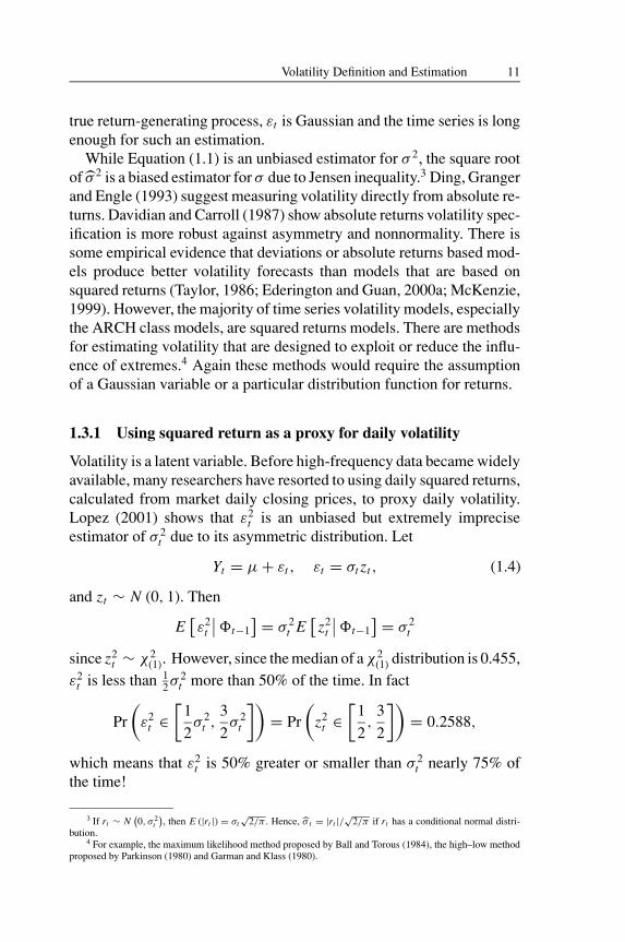
1.3.1 Using squared return as a proxy for daily volatility
Volatility is a latent variable. Before high-frequency data became widelyavailable, many researchers have resorted to using daily squared returns,calculated from market daily closing prices, to proxy daily volatility.Lopez (2001) shows that ε2
t is an unbiased but extremely impreciseestimator of σ 2
t due to its asymmetric distribution. Let
Yt = µ + εt , εt = σt zt , (1.4)
and zt ∼ N (0, 1). Then
E[ε2
t
∣∣�t−1] = σ 2
t E[
z2t
∣∣�t−1] = σ 2
t
since z2t ∼ χ2
(1). However, since the median of a χ2(1) distribution is 0.455,
ε2t is less than 1
2σ2t more than 50% of the time. In fact
Pr
(ε2
t ∈[
1
2σ 2
t ,3
2σ 2
t
])= Pr
(z2
t ∈[
1
2,
3
2
])= 0.2588,
which means that ε2t is 50% greater or smaller than σ 2
t nearly 75% ofthe time!
3 If rt ∼ N(0, σ 2
t
), then E (|rt |) = σt
√2/π . Hence, σ t = |rt |/
√2/π if rt has a conditional normal distri-
bution.4 For example, the maximum likelihood method proposed by Ball and Torous (1984), the high–low method
proposed by Parkinson (1980) and Garman and Klass (1980).

JWBK021-01 JWBK021-Poon March 15, 2005 13:28 Char Count= 0
12 Forecasting Financial Market Volatility
Under the null hypothesis that returns in (1.4) are generated by aGARCH(1,1) process, Andersen and Bollerslev (1998) show that thepopulation R2 for the regression
ε2t = α + βσ 2
t + υt
is equal to κ−1 where κ is the kurtosis of the standardized residuals and κ
is finite. For conditional Gaussian error, the R2 from a correctly specifiedGARCH(1,1) model cannot be greater than 1/3. For thick tail distribu-tion, the upper bound for R2 is lower than 1/3. Christodoulakis andSatchell (1998) extend the results to include compound normals and theGram–Charlier class of distributions confirming that the mis-estimationof forecast performance is likely to be worsened by nonnormality knownto be widespread in financial data.
Hence, the use of ε2t as a volatility proxy will lead to low R2 and under-
mine the inference on forecast accuracy. Blair, Poon and Taylor (2001)report an increase of R2 by three to four folds for the 1-day-ahead fore-cast when intraday 5-minutes squared returns instead of daily squaredreturns are used to proxy the actual volatility. The R2 of the regressionof |εt | on σ intra
t is 28.5%. Extra caution is needed when interpreting em-pirical findings in studies that adopt such a noisy volatility estimator.Figure 1.4 shows the time series of these two volatility estimates overthe 7-year period from January 1993 to December 1999. Although theoverall trends look similar, the two volatility estimates differ in manydetails.
1.3.2 Using the high–low measure to proxy volatility
The high–low, also known as the range-based or extreme-value, methodof estimating volatility is very convenient because daily high, low, open-ing and closing prices are reported by major newspapers, and the cal-culation is easy to program using a hand-held calculator. The high–lowvolatility estimator was studied by Parkinson (1980), Garman and Klass(1980), Beckers (1993), Rogers and Satchell (1991), Wiggins (1992),Rogers, Satchell and Yoon (1994) and Alizadeh, Brandt and Diebold(2002). It is based on the assumption that return is normally distributedwith conditional volatility σt . Let Ht and Lt denote, respectively, thehighest and the lowest prices on day t . Applying the Parkinson (1980)H -L measure to a price process that follows a geometric Brownian

JWBK021-01 JWBK021-Poon March 15, 2005 13:28 Char Count= 0
Volatility Definition and Estimation 13
(a) Conditional variance proxied by daily squared returns
0
0.01
0.02
0.03
0.04
0.05
0.06
0.07
0.08
04/01/1993 04/01/1994 04/01/1995 04/01/1996 04/01/1997 04/01/1998 04/01/1999
(b) Conditional variance derived as the sum of intraday squared returns
0
0.01
0.02
0.03
0.04
0.05
0.06
0.07
0.08
04/01/1993 04/01/1994 04/01/1995 04/01/1996 04/01/1997 04/01/1998 04/01/1999
Figure 1.4 S&P100 daily volatility for the period from January 1993 to December1999
motion results in the following volatility estimator (Bollen and Inder,2002):
σ 2t = (ln Ht − ln Lt )2
4 ln 2The Garman and Klass (1980) estimator is an extension of Parkinson(1980) where information about opening, pt−1, and closing, pt , pricesare incorporated as follows:
σ 2t = 0.5
(ln
Ht
Lt
)2
− 0.39
(ln
pt
pt−1
)2
.
We have already shown that financial market returns are not likely tobe normally distributed and have a long tail distribution. As the H -Lvolatility estimator is very sensitive to outliers, it will be useful to ap-ply the trimming procedures in Section 1.4. Provided that there are nodestabilizing large values, the H -L volatility estimator is very efficient
JWBK021-01 JWBK021-Poon March 15, 2005 13:28 Char Count= 0
14 Forecasting Financial Market Volatility
and, unlike the realized volatility estimator introduced in the next sec-tion, it is least affected by market microstructure effect.
1.3.3 Realized volatility, quadratic variation and jumps
More recently and with the increased availability of tick data, the termrealized volatility is now used to refer to volatility estimates calculatedusing intraday squared returns at short intervals such as 5 or 15 minutes.5
For a series that has zero mean and no jumps, the realized volatility con-verges to the continuous time volatility. To understand this, we assumefor the ease of exposition that the instantaneous returns are generated bythe continuous time martingale,
dpt = σt dWt , (1.5)
where dWt denotes a standard Wiener process. From (1.5) the con-ditional variance for the one-period returns, rt+1 ≡ pt+1 − pt , is∫ t+1
t σ 2s ds which is known as the integrated volatility over the period t
to t + 1. Note that while asset price pt can be observed at time t , thevolatility σt is an unobservable latent variable that scales the stochasticprocess dWt continuously through time.
Let m be the sampling frequency such that there are m continuouslycompounded returns in one unit of time and
rm,t ≡ pt − pt− 1/m (1.6)
and realized volatility
RVt+1 =∑
j=1,···,mr2
m,t+ j/m .
If the discretely sampled returns are serially uncorrelated and the samplepath for σt is continuous, it follows from the theory of quadratic variation(Karatzas and Shreve, 1988) that
p limm→∞
(∫ t+1
tσ 2
s ds −∑
j=1,···,mr2
m,t+ j/m
)= 0.
Hence time t volatility is theoretically observable from the sample pathof the return process so long as the sampling process is frequent enough.
5 See Fung and Hsieh (1991) and Andersen and Bollerslev (1998). In the foreign exchange markets, quotesfor major exchange rates are available round the clock. In the case of stock markets, close-to-open squared returnis used in the volatility aggregation process during market close.

JWBK021-01 JWBK021-Poon March 15, 2005 13:28 Char Count= 0
Volatility Definition and Estimation 15
When there are jumps in price process, (1.5) becomes
dpt = σt dWt + κt dqt ,
where dqt is a Poisson process with dqt = 1 corresponding to a jump attime t , and zero otherwise, and κt is the jump size at time t when thereis a jump. In this case, the quadratic variation for the cumulative returnprocess is then given by∫ t+1
tσ 2
s ds +∑
t<s≤t+1
κ2 (s) , (1.7)
which is the sum of the integrated volatility and jumps.In the absence of jumps, the second term on the right-hand side of (1.7)
disappears, and the quadratic variation is simply equal to the integratedvolatility. In the presence of jumps, the realized volatility continues toconverge to the quadratic variation in (1.7)
p limm→∞
(∫ t+1
tσ 2
s ds +∑
t<s≤t+1
κ2 (s) −m∑
j=1
r2m,t+ j/m
)= 0. (1.8)
Barndorff-Nielsen and Shephard (2003) studied the property of the stan-dardized realized bipower variation measure
BV [a,b]m,t+1 = m[(a+b)/2−1]
m−1∑j=1
∣∣rm,t+ j/m∣∣a ∣∣rm,t+ ( j+1)/m
∣∣b , a, b ≥ 0.
They showed that when jumps are large but rare, the simplest case wherea = b = 1,
µ−21 BV [1,1]
m,t+1 = µ−21
m−1∑j=1
∣∣rm,t+ j/m∣∣ ∣∣rm,t+ ( j+1)/m
∣∣ →∫ t+1
tσ 2
s ds
where µ1 = √2/π . Hence, the realized volatility and the realized
bipower variation can be substituted into (1.8) to estimate the jumpcomponent, κt . Barndorff-Nielsen and Shephard (2003) suggested im-posing a nonnegative constraint on κt . This is perhaps too restrictive.For nonnegative volatility, κt + µ−2
1 BVt > 0 will be sufficient.Characteristics of financial market data suggest that returns measured
at an interval shorter than 5 minutes are plagued by spurious serialcorrelation caused by various market microstructure effects includingnonsynchronous trading, discrete price observations, intraday periodic

JWBK021-01 JWBK021-Poon March 15, 2005 13:28 Char Count= 0
16 Forecasting Financial Market Volatility
volatility patterns and bid–ask bounce.6 Bollen and Inder (2002), Ait-Sahalia, Mykland and Zhang (2003) and Bandi and Russell (2004) havegiven suggestions on how to isolate microstructure noise from realizedvolatility estimator.
1.3.4 Scaling and actual volatility
The forecast of multi-period volatilityσT,T + j (i.e. for j period) is taken tobe the sum of individual multi-step point forecasts s
j=1hT + j |T . Thesemulti-step point forecasts are produced by recursive substitution andusing the fact that ε2
T +i |T = hT +i |T for i > 0 and ε2T +i |T = ε2
T +i forT + i ≤ 0. Since volatility of financial time series has complex struc-ture, Diebold, Hickman, Inoue and Schuermann (1998) warn that fore-cast estimates will differ depending on the current level of volatility,volatility structure (e.g. the degree of persistence and mean reversionetc.) and the forecast horizon.
If returns are i id (independent and identically distributed, or strictwhite noise), then variance of returns over a long horizon can be derivedas a simple multiple of single-period variance. But, this is clearly not thecase for many financial time series because of the stylized facts listed inSection 1.2. While a point forecast of σ T −1,T | t−1 becomes very noisyas T → ∞, a cumulative forecast, σ t,T | t−1, becomes more accuratebecause of errors cancellation and volatility mean reversion except whenthere is a fundamental change in the volatility level or structure.7
Complication in relation to the choice of forecast horizon is partlydue to volatility mean reversion. In general, volatility forecast accu-racy improves as data sampling frequency increases relative to forecasthorizon (Andersen, Bollerslev and Lange, 1999). However, for forecast-ing volatility over a long horizon, Figlewski (1997) finds forecast errordoubled in size when daily data, instead of monthly data, is used to fore-cast volatility over 24 months. In some cases, where application is ofvery long horizon e.g. over 10 years, volatility estimate calculated using
6 The bid–ask bounce for example induces negative autocorrelation in tick data and causes the realizedvolatility estimator to be upwardly biased. Theoretical modelling of this issue so far assumes the price processand the microstructure effect are not correlated, which is open to debate since market microstructure theorysuggests that trading has an impact on the efficient price. I am grateful to Frank de Jong for explaining this to meat a conference.
7 σ t,T | t−1 denotes a volatility forecast formulated at time t − 1 for volatility over the period from t to T . Inpricing options, the required volatility parameter is the expected volatility over the life of the option. The pricingmodel relies on a riskless hedge to be followed through until the option reaches maturity. Therefore the requiredvolatility input, or the implied volatility derived, is a cumulative volatility forecast over the option maturity andnot a point forecast of volatility at option maturity. The interest in forecasting σ t,T | t−1 goes beyond the risklesshedge argument, however.

JWBK021-01 JWBK021-Poon March 15, 2005 13:28 Char Count= 0
Volatility Definition and Estimation 17
weekly or monthly data is better because volatility mean reversion isdifficult to adjust using high frequency data. In general, model-basedforecasts lose supremacy when the forecast horizon increases with re-spect to the data frequency. For forecast horizons that are longer than6 months, a simple historical method using low-frequency data over aperiod at least as long as the forecast horizon works best (Alford andBoatsman, 1995; and Figlewski, 1997).
As far as sampling frequency is concerned, Drost and Nijman (1993)prove, theoretically and for a special case (i.e. the GARCH(1,1) process,which will be introduced in Chapter 4), that volatility structure should bepreserved through intertemporal aggregation. This means that whetherone models volatility at hourly, daily or monthly intervals, the volatilitystructure should be the same. But, it is well known that this is not thecase in practice; volatility persistence, which is highly significant indaily data, weakens as the frequency of data decreases. 8 This furthercomplicates any attempt to generalize volatility patterns and forecastingresults.
1.4 THE TREATMENT OF LARGE NUMBERS
In this section, I use large numbers to refer generally to extreme values,outliers and rare jumps, a group of data that have similar characteristicsbut do not necessarily belong to the same set. To a statistician, there arealways two ‘extremes’ in each sample, namely the minimum and themaximum. The H -L method for estimating volatility described in theprevious section, for example, is also called the extreme value method.We have also noted that these H -L estimators assume conditional dis-tribution is normal. In extreme value statistics, normal distribution is butone of the distributions for the tail. There are many other extreme valuedistributions that have tails thinner or thicker than the normal distribu-tion’s. We have known for a long time now that financial asset returns arenot normally distributed. We also know the standardized residuals fromARCH models still display large kurtosis (see McCurdy and Morgan,1987; Milhoj, 1987; Hsieh, 1989; Baillie and Bollerslev, 1989). Con-ditional heteroscedasticity alone could not account for all the tail thick-ness. This is true even when the Student-t distribution is used to construct
8 See Diebold (1988), Baillie and Bollerslev (1989) and Poon and Taylor (1992) for examples. Note thatNelson (1992) points out separately that as the sampling frequency becomes shorter, volatility modelled usingdiscrete time model approaches its diffusion limit and persistence is to be expected provided that the underlyingreturns is a diffusion or a near-diffusion process with no jumps.

JWBK021-01 JWBK021-Poon March 15, 2005 13:28 Char Count= 0
18 Forecasting Financial Market Volatility
the likelihood function (see Bollerslev, 1987; Hsieh, 1989). Hence, in theliterature, the extreme values and the tail observations often refer to thosedata that lie outside the (conditional) Gaussian region. Given that jumpsare large and are modelled as a separate component to the Brownianmotion, jumps could potentially be seen as a set similar to those tailobservations provided that they are truly rare.
Outliers are by definition unusually large in scale. They are so largethat some have argued that they are generated from a completely dif-ferent process or distribution. The frequency of occurrence should bemuch smaller for outliers than for jumps or extreme values. Outliersare so huge and rare that it is very unlikely that any modelling effortwill be able to capture and predict them. They have, however, undueinfluence on modelling and estimation (Huber, 1981). Unless extremevalue techniques are used where scale and marginal distribution are of-ten removed, it is advisable that outliers are removed or trimmed beforemodelling volatility. One such outlier in stock market returns is the Oc-tober 1987 crash that produced a 1-day loss of over 20% in stock marketsworldwide.
The ways that outliers have been tackled in the literature largely de-pend on their sizes, the frequency of their occurrence and whether theseoutliers have an additive or a multiplicative impact. For the rare andadditive outliers, the most common treatment is simply to remove themfrom the sample or omit them in the likelihood calculation (Kearns andPagan, 1993). Franses and Ghijsels (1999) find forecasting performanceof the GARCH model is substantially improved in four out of five stockmarkets studied when the additive outliers are removed. For the raremultiplicative outliers that produced a residual impact on volatility, adummy variable could be included in the conditional volatility equationafter the outlier returns has been dummied out in the mean equation(Blair, Poon and Taylor, 2001).
rt = µ + ψ1 Dt + εt , εt =√
ht zt
ht = ω + βht−1 + αε2t−1 + ψ2 Dt−1
where Dt is 1 when t refers to 19 October 1987 and 0 otherwise. Per-sonally, I find a simple method such as the trimming rule in (1.2) veryquick to implement and effective.
The removal of outliers does not remove volatility persistence. In fact,the evidence in the previous section shows that trimming the data using(1.2) actually increases the ‘long memory’ in volatility making it appear

JWBK021-01 JWBK021-Poon March 15, 2005 13:28 Char Count= 0
Volatility Definition and Estimation 19
to be extremely persistent. Since autocorrelation is defined as
ρ (rt , rt−τ ) = Cov (rt , rt−τ )
V ar (rt ),
the removal of outliers has a great impact on the denominator, reducesV ar (rt ) and increases the individual and the cumulative autocorrelationcoefficients.
Once the impact of outliers is removed, there are different views abouthow the extremes and jumps should be handled vis-a-vis the rest of thedata. There are two schools of thought, each proposing a seeminglydifferent model, and both can explain the long memory in volatility. Thefirst believes structural breaks in volatility cause mean level of volatilityto shift up and down. There is no restriction on the frequency or the sizeof the breaks. The second advocates the regime-switching model wherevolatility switches between high and low volatility states. The means ofthe two states are fixed, but there is no restriction on the timing of theswitch, the duration of each regime and the probability of switching.Sometimes a three-regime switching is adopted but, as the number ofregimes increases, the estimation and modelling become more complex.Technically speaking, if there are infinite numbers of regimes then thereis no difference between the two models. The regime-switching modeland the structural break model will be described in Chapter 5.

JWBK021-02 JWBK021-Poon March 14, 2005 23:4 Char Count= 0
2
Volatility Forecast Evaluation
Comparing forecasting performance of competing models is one of themost important aspects of any forecasting exercise. In contrast to theefforts made in the construction of volatility models and forecasts, littleattention has been paid to forecast evaluation in the volatility forecastingliterature. Let Xt be the predicted variable, Xt be the actual outcome andεt = Xt − Xt be the forecast error. In the context of volatility forecast,Xt and Xt are the predicted and actual conditional volatility. There aremany issues to consider:
(i) The form of Xt : should it be σ 2t or σt ?
(ii) Given that volatility is a latent variable, the impact of the noiseintroduced in the estimation of Xt , the actual volatility.
(iii) Which form of εt is more relevant for volatility model selection; ε2
t , |εt | or |εt |/Xt ? Do we penalize underforecast, Xt < Xt ,more than overforecast, Xt > Xt ?
(iv) Given that all error statistics are subject to noise, how do we knowif one model is truly better than another?
(v) How do we take into account when Xt and Xt+1 (and similarly forεt and Xt ) cover a large amount of overlapping data and are seriallycorrelated?
All these issues will be considered in the following sections.
2.1 THE FORM OF Xt
Here we argue that Xt should be σt , and that if σt cannot be estimatedwith some accuracy it is best not to perform comparison across predictivemodels at all. The practice of using daily squared returns to proxy dailyconditional variance has been shown time and again to produce wrongsignals in model selection.
Given that all time series volatility models formulate forecasts basedon past information, they are not designed to predict shocks that are new
21

JWBK021-02 JWBK021-Poon March 14, 2005 23:4 Char Count= 0
22 Forecasting Financial Market Volatility
to the system. Financial market volatility has many stylized facts. Oncea shock has entered the system, the merit of the volatility model dependson how well it captures these stylized facts in predicting the volatility ofthe following days. Hence we argue that Xt should be σt . Conditionalvariance σ 2
t formulation gives too much weight to the errors caused by‘new’ shocks and especially the large ones, distorting the less extremeforecasts where the models are to be assessed.
Note also that the square of a variance error is the fourth power ofthe same error measured from standard deviation. This can complicatethe task of forecast evaluation given the difficulty in estimating fourthmoments with common distributions let alone the thick-tailed ones infinance. The confidence interval of the mean error statistic can be verywide when forecast errors are measured from variances and worse if theyare squared. This leads to difficulty in finding significant differencesbetween forecasting models.
Davidian and Carroll (1987) make similar observations in their studyof variance function estimation for heteroscedastic regression. Usinghigh-order theory, they show that the use of square returns for modellingvariance is appropriate only for approximately normally distributed data,and becomes nonrobust when there is a small departure from normal-ity. Estimation of the variance function that is based on logarithmictransformation or absolute returns is more robust against asymmetryand nonnormality.
Some have argued that perhaps Xt should be lnσt to rescale the size ofthe forecast errors (Pagan and Schwert, 1990). This is perhaps one steptoo far. After all, the magnitude of the error directly impacts on optionpricing, risk management and investment decision. Taking the logarithmof the volatility error is likely to distort the loss function which is directlyproportional to the magnitude of forecast error. A decision maker mightbe more risk-averse towards the larger errors.
We have explained in Section 1.3.1 the impact of using squared returnsto proxy daily volatility. Hansen and Lunde (2004b) used a series ofsimulations to show that ‘. . . the substitution of a squared return forthe conditional variance in the evaluation of ARCH-type models canresult in an inferior model being chosen as [the] best with a probabilityconverges to one as the sample size increases . . . ’. Hansen and Lunde(2004a) advocate the use of realized volatility in forecast evaluation butcaution the noise introduced by market macrostructure when the intradayreturns are too short.

JWBK021-02 JWBK021-Poon March 14, 2005 23:4 Char Count= 0
Volatility Forecast Evaluation 23
2.2 ERROR STATISTICS AND THE FORM OF εt
Ideally an evaluation exercise should reflect the relative or absolute use-fulness of a volatility forecast to investors. However, to do that oneneeds to know the decision process that require these forecasts and thecosts and benefits that result from using better forecasts. Utility-basedcriteria, such as that used in West, Edison and Cho (1993), require someassumptions about the shape and property of the utility function. In prac-tice these costs, benefits and utility function are not known and one oftenresorts to simply use measures suggested by statisticians.
Popular evaluation measures used in the literature includeMean Error (ME)
1
N
N∑t=1
εt = 1
N
N∑t=1
(σ t − σt ) ,
Mean Square Error (MSE)
1
N
N∑t=1
ε2t = 1
N
N∑t=1
(σ t − σt )2 ,
Root Mean Square Error (RMSE)√√√√ 1
N
N∑t=1
ε2t =
√√√√ 1
N
N∑t=1
(σ t − σt )2,
Mean Absolute Error (MAE)
1
N
N∑t=1
|εt | = 1
N
N∑t=1
|σ t − σt | ,
Mean Absolute Percent Error (MAPE)
1
N
N∑t=1
|εt |σt
= 1
N
N∑t=1
|σ t − σt |σt
.
Bollerslev and Ghysels (1996) suggested a heteroscedasticity-adjusted version of MSE called HMSE where
HMSE = 1
N
N∑t=1
[σt
σ t− 1
]2

JWBK021-02 JWBK021-Poon March 14, 2005 23:4 Char Count= 0
24 Forecasting Financial Market Volatility
This is similar to squared percentage error but with the forecast errorscaled by predicted volatility. This type of performance measure is notappropriate if the absolute magnitude of the forecast error is a majorconcern. It is not clear why it is the predicted and not the actual volatilitythat is used in the denominator. The squaring of the error again will givegreater weight to large errors.
Other less commonly used measures include mean logarithm of ab-solute errors (MLAE) (as in Pagan and Schwert, 1990), the Theil-Ustatistic and one based on asymmetric loss function, namely LINEX:Mean Logarithm of Absolute Errors (MLAE)
1
N
N∑t=1
ln |εt | = 1
N
N∑t=1
ln |σ t − σt |
Theil-U measure
Theil-U =
N∑t=1
(σ t − σt )2
N∑t=1
(σ B M
t − σt)2
, (2.1)
where σ B Mt is the benchmark forecast, used here to remove the effect of
any scalar transformation applied to σt .LINEX has asymmetric loss function whereby the positive errors are
weighted differently from the negative errors:
LINEX = 1
N
N∑t=1
[exp {−a (σ t − σt )} + a (σ t − σt ) − 1]. (2.2)
The choice of the parameter a is subjective. If a > 0, the function isapproximately linear for overprediction and exponential for underpre-diction. Granger (1999) describes a variety of other asymmetric lossfunctions of which the LINEX is an example. Given that most investorswould treat gains and losses differently, the use of asymmetric loss func-tions may be advisable, but their use is not common in the literature.
2.3 COMPARING FORECAST ERRORSOF DIFFERENT MODELS
In the special case where the error distribution of one forecastingmodel dominates that of another forecasting model, the comparison is

JWBK021-02 JWBK021-Poon March 14, 2005 23:4 Char Count= 0
Volatility Forecast Evaluation 25
straightforward (Granger, 1999). In practice, this is rarely the case, andmost comparisons of forecasting results are made based on the errorstatistics described in Section 2.2. It is important to note that these er-ror statistics are themselves subject to error and noise. So if an errorstatistic of model A is higher than that of model B, one cannot concludethat model B is better than A without performing tests of significance.For statistical inference, West (1996), West and Cho (1995) and Westand McCracken (1998) show how standard errors for ME, MSE, MAEand RMSE may be derived taking into account serial correlation in theforecast errors and uncertainty inherent in volatility model parameterestimates.
If there are T number of observations in the sample and T is large,there are two ways in which out-of-sample forecasts may be made.Assume that we use n number of observations for estimation and makeT − n number of forecasts. The recursive scheme starts with the sample{1, · · · , n} and makes first forecast at n + 1. The second forecast forn + 2 will include the last observation and form the information set{1, · · · , n + 1}. It follows that the last forecast for T will include allbut the last observation, i.e. the information set is {1, · · · , T − 1}. Inpractice, the rolling scheme is more popular, where a fixed number ofobservations is used in the estimation. So the forecast for n + 2 will bebased on information set {2, · · · , n + 1}, and the last forecast at T will bebased on {T − n, · · · , T − 1}. The rolling scheme omits information inthe distant past. It is also more manageable in terms of computation whenT is very large. The standard errors developed by West and co-authorsare based on asymptotic theory and work for recursive scheme only. Forsmaller sample and rolling scheme forecasts, Diebold and Mariano’s(1995) small sample methods are more appropriate.
Diebold and Mariano (1995) propose three tests for ‘equal accuracy’between two forecasting models. The tests relate prediction error tosome very general loss function and analyse loss differential derivedfrom errors produced by two competing models. The three tests includean asymptotic test that corrects for series correlation and two exact fi-nite sample tests based on sign test and the Wilcoxon sign-rank test.Simulation results show that the three tests are robust against non-Gaussian, nonzero mean, serially and contemporaneously correlatedforecast errors. The two sign-based tests in particular continue to workwell among small samples. The Diebold and Mariano tests have beenused in a number of volatility forecasting contests. We provide the testdetails here.

JWBK021-02 JWBK021-Poon March 14, 2005 23:4 Char Count= 0
26 Forecasting Financial Market Volatility
Let {Xi t}Tt=1 and {X j t}T
t=1 be two sets of forecasts for {Xt}Tt=1 from
models i and j respectively. Let the associated forecast errors be {eit}Tt=1
and {e jt}Tt=1. Let g (·) be the loss function (e.g. the error statistics in
Section 2.2) such that
g(Xt , Xi t
) = g (eit ) .
Next define loss differential
dt ≡ g (eit ) − g(e jt
).
The null hypothesis is equal forecast accuracy and zero loss differentialE(dt ) = 0.
2.3.1 Diebold and Mariano’s asymptotic test
The first test targets on the mean
d = 1
T
T∑t=1
|g(eit ) − g(e jt )|
with test statistic
S1 = d√1
T2π fd (0)
S1 ∼ N (0, 1)
2π fd (0) =T −1∑
τ=−(T −1)
1
(τ
S (T )
)γ d (τ )
γ d (τ ) = 1
T
T∑t=|τ |+1
(dt − d
) (dt−|τ | − d
).
The operator 1 (τ/S (T )) is the lag window, and S (T ) is the truncationlag with
1
(τ
S (T )
)=
1 for
∣∣∣∣ τ
S (T )
∣∣∣∣ ≤ 1
0 otherwise.
Assuming that k-step ahead forecast errors are at most (k − 1)-dependent, it is therefore recommended that S (T ) = (k − 1). It is notlikely that fd (0) will be negative, but in the rare event that fd (0) < 0,

JWBK021-02 JWBK021-Poon March 14, 2005 23:4 Char Count= 0
Volatility Forecast Evaluation 27
it should be treated as zero and the null hypothesis of equal forecastaccuracy be rejected automatically.
2.3.2 Diebold and Mariano’s sign test
The sign test targets on the median with the null hypothesis that
Med (d) = Med(g(eit ) − g
(e jt
))= 0.
Assuming that dt ∼ iid, then the test statistic is
S2 =T∑
t=1
I+ (dt )
where
I+ (dt ) ={
1 if dt > 00 otherwise
.
For small sample, S2 should be assessed using a table for cumulativebinomial distribution. In large sample, the Studentized verson of S2 isasymptotically normal
S2a = S2 − 0.5T√0.25T
a∼ N (0, 1).
2.3.3 Diebold and Mariano’s Wilcoxon sign-rank test
As the name indicates, this test is based on both the sign and the rank ofloss differential with test statistic
S3 =T∑
t=1
I+ (dt ) rank (|dt |)
represents the sum of the ranks of the absolute values of the positiveobservations. The critical values for S3 have been tabulated for smallsample. For large sample, the Studentized verson of S3 is again asymp-totically normal
S2a =S3 − T (T + 1)
4√T (T + 1) (2T + 1)
24
a∼ N (0, 1) .

JWBK021-02 JWBK021-Poon March 14, 2005 23:4 Char Count= 0
28 Forecasting Financial Market Volatility
2.3.4 Serially correlated loss differentials
Serial correlation is explicitly taken care of in S1. For S2 and S3 (andtheir asymptotic counter parts S2a and S3a), the following k-set of lossdifferentials have to be tested jointly{
di j,1, di j,1+k, di j,1+2k, · · ·},{
di j,2, di j,2+k, di j,2+2k, · · ·},
...{di j,k, di j,2k, di j,3k, · · ·
}.
A test with size bounded by α is then tested k times, each of size α/k,on each of the above k loss-differentials sequences. The null hypothesisof equal forecast accuracy is rejected if the null is rejected for any of thek samples.
2.4 REGRESSION-BASED FORECAST EFFICIENCYAND ORTHOGONALITY TEST
The regression-based method for examining the informational contentof forecasts is by far the most popular method in volatility forecasting.It involves regressing the actual volatility, Xt , on the forecasts literature,Xt , as shown below:
Xt = α + β Xt + υt . (2.3)
Conditioning upon the forecast, the prediction is unbiased only if α = 0and β = 1.
Since the error term, υt , is heteroscedastic and serially correlated whenoverlapping forecasts are evaluated, the standard errors of the parameterestimates are often computed on the basis of Hansen and Hodrick (1980).Let Y be the row matrix of regressors including the constant term. In(2.3), Yt = (
1 Xt)
is a 1 × 2 matrix. Then
� = T −1T∑
t=1
υ2t Y
′t Yt
+T −1T∑
k=1
T∑t=k+1
Q (k, t) υkυt
(Y
′t Yk + Y
′kYt
),

JWBK021-02 JWBK021-Poon March 14, 2005 23:4 Char Count= 0
Volatility Forecast Evaluation 29
where υk and υt are the residuals for observation k and t from the regres-sion. The operator Q (k, t) is an indicator function taking the value 1 ifthere is information overlap between Yk and Yt . The adjusted covariancematrix for the regression coefficients is then calculated as
� =(
Y′Y)−1
�(
Y′Y)−1
. (2.4)
Canina and Figlewski (1993) conducted some simulatation studies andfound the corrected standard errors in (2.4) are close to the true values,and the use of overlapping data reduced the standard error between one-quarter and one-eighth of what would be obtained with only nonover-lapping data.
In cases where there are more than one forecasting model, additionalforecasts are added to the right-hand side of (2.3) to check for incremen-tal explanatory power. Such a forecast encompassing test dates backto Theil (1966). Chong and Hendry (1986) and Fair and Shiller (1989,1990) provide further theoretical exposition of such methods for testingforecast efficiency. The first forecast is said to subsume information con-tained in other forecasts if these additional forecasts do not significantlyincrease the adjusted regression R2. Alternatively, an orthogonality testmay be conducted by regressing the residuals from (2.3) on other fore-casts. If these forecasts are orthogonal, i.e. do not contain additionalinformation, then the regression coefficients will not be different fromzero.
While it is useful to have an unbiased forecast, it is important todistinguish between bias and predictive power. A biased forecast canhave predictive power if the bias can be corrected. An unbiased forecastis useless if all forecast errors are big. For Xi to be considered as a goodforecast, Var(υt ) should be small and R2 for the regression should tendto 100%. Blair, Poon and Taylor (2001) use the proportion of explainedvariability, P , to measure explanatory power
P = 1 −∑(
Xi − Xi)2∑
(Xi − µX )2. (2.5)
The ratio in the right-hand side of (2.5) compares the sum of squaredprediction errors (assuming α = 0 and β = 1 in (2.3)) with the sumof squared variation of Xi . P compares the amount of variation in theforecast errors with that in actual volatility. If prediction errors are small,

JWBK021-02 JWBK021-Poon March 14, 2005 23:4 Char Count= 0
30 Forecasting Financial Market Volatility
P is closer to 1. Given that a regression model that produces (2.5) is morerestrictive than (2.3), P is likely to be smaller than conventional R2. Pcan even be negative since the ratio on the right-hand side of (2.5) canbe greater than 1. A negative P means that the forecast errors havea greater amount of variation than the actual volatility, which is not adesirable characteristic for a well-behaved forecasting model.
2.5 OTHER ISSUES IN FORECAST EVALUATION
In all forecast evaluations, it is important to distinguish in-sample andout-of-sample forecasts. In-sample forecast, which is based on param-eters estimated using all data in the sample, implicitly assumes parameterestimates are stable across time. In practice, time variation of parameterestimates is a critical issue in forecasting. A good forecasting modelshould be one that can withstand the robustness of out-of-sample test –a test design that is closer to reality.
Instead of striving to make some statistical inference, model perfor-mance could be judged on some measures of economic significance. Ex-amples of such an approach include portfolio improvement derived frombetter volatility forecasts (Fleming, Kirby and Ostdiek, 2000, 2002).Some papers test forecast accuracy by measuring the impact on optionpricing errors (Karolyi, 1993). In the latter case, pricing error in theoption model will be cancelled out when the option implied volatility isreintroduced into the pricing formula. So it is not surprising that evalu-ation which involves comparing option pricing errors often prefers theimplied volatility method to all other time series methods.
Research in financial market volatility has been concentrating onmodelling and less on forecasting. Work on combined forecast is rare,probably because the groups of researchers in time series models andoption pricing do not seem to mix. What has not yet been done in theliterature is to separate the forecasting period into ‘normal’ and ‘excep-tional’ periods. It is conceivable that different forecasting methods arebetter suited to different trading environment and economic conditions.

JWBK021-03 JWBK021-Poon March 4, 2005 12:43 Char Count= 0
3
Historical Volatility Models
Compared with the other types of volatility models, the historical volatil-ity models (HIS) are the easiest to manipulate and construct. The well-known Riskmetrics EWMA (equally weighted moving average) modelfrom JP Morgan is a form of historical volatility model; so are modelsthat build directly on realized volatility that have became very popu-lar in the last few years. Historical volatility models have been shownto have good forecasting performance compared with other time seriesvolatility models. Unlike the other two time series models (viz. ARCHand stochastic volatility (SV)) conditional volatility is modelled sepa-rately from returns in the historical volatility models, and hence theyare less restrictive and are more ready to respond to changes in volatil-ity dynamic. Studies that find historical volatility models forecast betterthan ARCH and/or SV models include Taylor (1986, 1987), Figlewski(1997), Figlewski and Green (1999), Andersen, Bollerslev, Diebold andLabys (2001) and Taylor, J. (2004). With the increased availability ofintraday data, we can expect to see research on the realized volatilityvariant of the historical model to intensify in the next few years.
3.1 MODELLING ISSUES
Unlike ARCH SV models where returns are the main input, HIS modelsdo not normally use returns information so long as the volatility estimatesare ready at hand. Take the simplest form of ARCH(1) for example,
rt = µ + εt , εt ∼ N (0, σt ) (3.1)
εt = ztσt , zt ∼ N (0, 1)
σ 2t = ω + α1ε
2t−1. (3.2)
The conditional volatility σ 2t in (3.2) is modelled as a ‘byproduct’
of the return equation (3.1). The estimation is done by maximizingthe likelihood of observing {εt} using the normal, or other chosen,density. The construction and estimation of SV models are similar tothose of ARCH, except that there is now an additional innovation termin (3.2).
31

JWBK021-03 JWBK021-Poon March 4, 2005 12:43 Char Count= 0
32 Forecasting Financial Market Volatility
In contrast, the HIS model is built directly on conditional volatility,e.g. an AR(1) model:
σt = γ + β1σt−1 + υt . (3.3)
The parameters γ and β1 are estimated by minimizing in-sample forecasterrors, υt , where
υt = σt − γ − β1σ t−1,
and the forecaster has the choice of reducing mean square errors, meanabsolute errors etc., as in the case of choosing an appropriate forecasterror statistic in Section 2.2.
The historical volatility estimates σt in (3.3) can be calculated assample standard deviations if there are sufficient data for each t in-terval. If there is not sufficient information, then the H -L method ofSection 1.3.2 may be used, and in the most extreme case, where onlyone observation is available for each t interval, one often resorts to usingabsolute return to proxy for volatility at t . In Section 1.3.1 we have high-lighted the danger of using daily absolute or squared returns to proxy‘actual’ daily volatility for the purpose of forecast evaluation, as thiscould lead to very misleading model ranking. The problem with the useof daily absolute return in volatility modelling is less severe providedthat long distributed lags are included (Nelson, 1992; Nelson and Foster,1995). With the increased availability of intraday data, historical volatil-ity estimates can be calculated quite accurately as realized volatilityfollowing Section 1.3.3.
3.2 TYPES OF HISTORICAL VOLATILITY MODELS
There are now two major types of HIS models: the single-state and theregime-switching models. All the HIS models differ by the number of lagvolatility terms included in the model and the weights assigned to them,reflecting the choice on the tradeoff between increasing the amount ofinformation and more updated information.
3.2.1 Single-state historical volatility models
The simplest historical price model is the random walk model, wherethe difference between consecutive period volatility is modelled as arandom noise;
σt = σt−1 + vt ,

JWBK021-03 JWBK021-Poon March 4, 2005 12:43 Char Count= 0
Historical Volatility Models 33
So the best forecast for tomorrow’s volatility is today’s volatility:
σ t+1 = σt ,
where σt alone is used as a forecast for σt+1.In contrast, the historical average method makes a forecast based on
the entire history
σ t+1 = 1
t(σt + σt−1 + · · · + σ1) .
The simple moving average method below,
σ t+1 = 1
τ(σt + σt−1 + · · · + σt−τ−1) ,
is similar to the historical average method, except that older informationis discarded. The value of τ (i.e. the lag length to past informationused) could be subjectively chosen or based on minimizing in-sampleforecast error, ςt+1 = σt+1 − σ t+1. The multi-period forecasts σ t+τ forτ > 1 will be the same as the one-step-ahead forecast σ t+1 for all threemethods above.
The exponential smoothing method below,
σt = (1 − β) σt−1 + βσ t−1 + ξt and 0 ≤ β ≤ 1,
σ t+1 = (1 − β) σt + βσ t ,
is similar to the historical method, but more weight is given to the recentpast and less weight to the distant past. The smoothing parameter β isestimated by minimizing the in-sample forecast errors ξt .
The exponentially weighted moving average method (EWMA) belowis the moving average method with exponential weights:
σ t+1 =τ∑
i=1
β i σt−i−1
/ τ∑i=1
β i .
Again the smoothing parameter β is estimated by minimizing the in-sample forecast errors ξt . The JP Morgan RiskmetricsTM model is aprocedure that uses the EWMA method.
All the historical volatility models above have a fixed weightingscheme or a weighting scheme that follows some declining pattern. Othertypes of historical model have weighting schemes that are not prespec-ified. The simplest of such models is the simple regression method,
σt = γ + β1 σt−1 + β2 σt−2 + · · · + βn σt−n + υt ,
σ t+1 = γ + β1 σt + β2 σt−1 + · · · + βn σt−n+1,

JWBK021-03 JWBK021-Poon March 4, 2005 12:43 Char Count= 0
34 Forecasting Financial Market Volatility
which expresses volatility as a function of its past values and an errorterm.
The simple regression method is principally autoregressive. If pastvolatility errors are also included, one gets the ARMA model
σ t+1 = β1 σt + β2 σt−1 + · · · + γ1 υt + γ2 υt−1 + · · · .Introducing a differencing order I(d), we get ARIMA when d = 1 andARFIMA when d < 1.
3.2.2 Regime switching and transition exponential smoothing
In this section, we have the threshold autoregressive model from Caoand Tsay (1992):
σt = φ(i)0 + φ
(i)1 σt−1 + · · · + φ(i)
p σt−p + vt , i = 1, 2, . . . , k
σ t+1 = φ(i)0 + φ
(i)1 σt + · · · + φ(i)
p σt+1−p,
where the thresholds separate volatility into states with independentsimple regression models and noise processes in each state. The predic-tion σ t+1 could be based solely on current state information i assumingthe future will remain on current state. Alternatively it could be based oninformation of all states weighted by the transition probability for eachstate. Cao and Tsay (1992) found the threshold autoregressive modeloutperformed EGARCH and GARCH in forecasting of the 1- to 30-month volatility of the S&P value-weighted index. EGARCH providedbetter forecasts for the S&P equally weighted index, possibly becausethe equally weighted index gives more weights to small stocks wherethe leverage effect could be more important.
The smooth transition exponential smoothing model is from Taylor,J. (2004):
σ t = αt−1ε2t−1 + (1 − αt−1) σ 2
t−1 + vt , (3.4)
where
αt−1 = 1
1 + exp (β + γ Vt−1),
and Vt−1 = aεt−1 + b |εt−1| is the transition variable. The smoothingparameter αt−1 varies between 0 and 1, and its value depends on thesize and the sign of εt−1. The dependence on εt−1 means that multi-step-ahead forecasts cannot be made except through simulation. (The samewould apply to many nonlinear ARCH and SV models as we will showin the next few chapters.)

JWBK021-03 JWBK021-Poon March 4, 2005 12:43 Char Count= 0
Historical Volatility Models 35
One-day-ahead forecasting results show that the smooth transition ex-ponential smoothing model performs very well against several ARCHcounterparts and even outperformed, on a few occasions, the realizedvolatility forecast. But these rankings were not tested for statistical sig-nificance, so it is difficult to come to a conclusion given the closenessof many error statistics reported.
3.3 FORECASTING PERFORMANCE
Taylor (1987) was one of the earliest to test time-series volatility fore-casting models before ARCH/GARCH permeated the volatility litera-ture. Taylor (1987) used extreme value estimates based on high, low andclosing prices to forecast 1 to 20 days DM/$ futures volatility and founda weighted average composite forecast performed best. Wiggins (1992)also gave support to extreme-value volatility estimators.
In the pre-ARCH era, there were many studies that covered a widerange of issues. Sometimes forecasters would introduce ‘learning’ byallowing parameters and weights of combined forecasts to be dynam-ically updated. These frequent updates did not always lead to betterresults, however. Dimson and Marsh (1990) found ex ante time-varyingoptimized weighting schemes do not always work well in out-of-sampleforecasts. Sill (1993) found S&P500 volatility was higher during reces-sion and that commercial T-Bill spread helped to predict stock-marketvolatility.
The randow walk and historical average method seems naive at first,but they seem to work very well for medium and long horizon forecasts.For forecast horizons that are longer than 6 months, low-frequency dataover a period at least as long as the forecast horizon works best. Toprovide equity volatility for investment over a 5-year period for exam-ple, Alford and Boatsman (1995) recommended, after studying a sam-ple of 6879 stocks, that volatility should be estimated from weekly ormonthly returns from the previous 5 years and that adjustment madebased on industry and company size. Figlewski (1997) analysed thevolatility of the S&P500, the long- and short-term US interest rate andthe Deutschemark–dollar exchange rate and the use of monthly dataover a long period provides the best long-horizon forecast. Alford andBoatsman (1995), Figlewski (1997) and Figlewski and Green (1999) allstressed the importance of having a long enough estimation period tomake good volatility forecasts over long horizon.

JWBK021-04 JWBK021-Poon March 14, 2005 23:5 Char Count= 0
4
ARCH
Financial market volatility is known to cluster. A volatile period tends topersist for some time before the market returns to normality. The ARCH(AutoRegressive Conditional Heteroscedasticity) model proposed byEngle (1982) was designed to capture volatility persistence in inflation.The ARCH model was later found to fit many financial time series and itswidespread impact on finance has led to the Nobel Committee’s recog-nition of Rob Engle’s work in 2003. The ARCH effect has been shownto lead to high kurtosis which fits in well with the empirically observedtail thickness of many asset return distributions. The leverage effect, aphenomenon related to high volatility brought on by negative return,is often modelled with a sign-based return variable in the conditionalvolatility equation.
4.1 ENGLE (1982)
The ARCH model, first introduced by Engle (1982), has been ex-tended by many researchers and extensively surveyed in Bera andHiggins (1993), Bollerslev, Chou and Kroner (1992), Bollerslev,Engle and Nelson (1994) and Diebold and Lopez (1995). In contrast tothe historical volatility models described in the previous chapter, ARCHmodels do not make use of the past standard deviations, but formulateconditional variance, ht , of asset returns via maximum likelihood pro-cedures. (We follow the ARCH literature here by writing σ 2
t = ht .) Toillustrate this, first write returns, rt , as
rt = µ + εt ,
εt =√
ht zt , (4.1)
where zt ∼ D (0, 1) is a white noise. The distribution D is often taken asnormal. The process zt is scaled by ht , the conditional variance, whichin turn is a function of past squared residual returns. In the ARCH(q)process proposed by Engle (1982),
ht = ω +q∑
j=1
α jε2t− j (4.2)
37

JWBK021-04 JWBK021-Poon March 14, 2005 23:5 Char Count= 0
38 Forecasting Financial Market Volatility
with ω > 0 and α j ≥ 0 to ensure ht is strictly positive variance. Typi-cally, q is of high order because of the phenomenon of volatility per-sistence in financial markets. From the way in which volatility is con-structed in (4.2), ht is known at time t − 1. So the one-step-ahead forecastis readily available. The multi-step-ahead forecasts can be formulatedby assuming E
[ε2
t+τ
] = ht+τ .The unconditional variance of rt is
σ 2 = ω
1 −q∑
j=1
α j
.
The process is covariance stationary if and only if the sum of the autore-gressive parameters is less than one
∑qj=1 α j < 1.
4.2 GENERALIZED ARCH
For high-order ARCH(q) process, it is more parsimonious to modelvolatility as a GARCH(p, q) (generalized ARCH due to Bollerslev(1986) and Taylor (1986)), where additional dependencies are permittedon p lags of past ht as shown below:
ht = ω +p∑
i=1
βi ht−i +q∑
j=1
α jε2t− j
and ω > 0. For GARCH(1, 1), the constraints α1 ≥ 0 and β1 ≥ 0 areneeded to ensure ht is strictly positive. For higher orders of GARCH,the constraints on βi and α j are more complex (see Nelson and Cao(1992) for details). The unconditional variance equals
σ 2 = ω
1 −p∑
i=1
βi −q∑
j=1
α j
The GARCH(p, q) model is covariance stationary if and only if∑pi=1 βi + ∑q
j=1 α j < 1.Volatility forecasts from GARCH(1, 1) can be made by repeated sub-
stitutions. First, we make use of the relationship (4.1) to provide anestimate for the expected squared residuals
E[ε2
t
] = ht E[z2
t
] = ht .

JWBK021-04 JWBK021-Poon March 14, 2005 23:5 Char Count= 0
Arch 39
The conditional variance ht+1 and the one-step-ahead forecast is knownat time t ,
ht+1 = ω + α1ε2t + β1ht . (4.3)
The forecast of ht+2 makes use of the fact that E[ε2
t+1
] = ht+1 and weget
ht+2 = ω + α1ε2t+1 + β1ht+1
= ω + (α1 + β1) ht+1.
Similarly,
ht+3 = ω + (α1 + β1) ht+2
= ω + ω (α1 + β1) + (α1 + β1)2 ht+1
= ω + ω (α1 + β1) + ω (α1 + β1)2 + (α1 + β1)2[α1ε
2t + β1ht
].
As the forecast horizon τ lengthens,
ht+τ = ω
1 − (α1 + β1)+ (α1 + β1)τ
[α1ε
2t + β1ht
]. (4.4)
If α1 + β1 < 1, the second term on the RHS of (4.4) dies out eventuallyand ht+τ converges to ω/[1 − (α1 + β1)], the unconditional variance.
If we write υt = ε2t − ht and substitute ht = ε2
t − υt into (4.3), weget
ε2t − υt = ω + α1ε
2t−1 + β1ε
2t−1 − β1υt−1
ε2t = ω + (α1 + β1) ε2
t−1 + υt − β1υt−1. (4.5)
Hence, ε2t , the squared residual returns follow an ARMA process with
autoregressive parameter (α1 + β1). If α1 + β1 is close to 1, the autore-gressive process in (4.5) dies out slowly.
4.3 INTEGRATED GARCH
For a GARCH(p, q) process, when∑p
i=1 αi + ∑qj=1 β j = 1, the un-
conditional variance σ 2 → ∞ is no longer definite. The series rt is notcovariance stationary, although it remains strictly stationary and ergodic.The conditional variance is then described as an integrated GARCH (de-noted as IGARCH) and there is no finite fourth moment.1
1 This is not the same as, and should not be confused with, the ‘integrated volatility’ described in Section 1.3.3.

JWBK021-04 JWBK021-Poon March 14, 2005 23:5 Char Count= 0
40 Forecasting Financial Market Volatility
An infinite volatility is a concept rather counterintuitive to real phe-nomena in economics and finance. Empirical findings suggest thatGARCH(1, 1) is the most popular structure for many financial timeseries. It turns out that RiskmetricsTM EWMA (exponentially weightedmoving average) is a nonstationary version of GARCH(1, 1) where thepersistence parameters, α1 and β1, sum to 1. To see the parallel, we firstmake repeated substitution of (4.3) and obtain
ht+2 = ω + αε2t+1 + βht+1
= ω + ωβ + αε2t+1 + αβε2
t + β2ht ,
ht+τ = ω
τ∑i=1
β i−1 + α
τ∑i=1
β i−1ε2t+τ−1 + βτ ht .
When τ → ∞, and provided that β < 1 we can infer that
ht = ω
1 − β+ α
∞∑i=1
β i−1ε2t−i . (4.6)
Next, we have the EWMA model for the sample standard deviations,where
σ 2t =
(1
1 + λ + λ2 + · · · + λn
) (σ 2
t−1 + λσ 2t−1 + · · · + λnσ 2
t−n
).
As n → ∞, and provided that λ < 1
σ 2t = (1 − λ)
∞∑i=1
λi−1σ 2t−i . (4.7)
If we view ε2t as a proxy for σ 2
t , (4.6) and (4.7) are both autoregressiveseries with long distributed lags, except that (4.6) has a constant termand (4.7) has not.2
While intuitively unconvincing as a volatility process because of theinfinite variance, the EWMA model has nevertheless been shown to bepowerful in volatility forecasting as it is not constrained by a mean levelof volatility (unlike e.g. the GARCH(1, 1) model), and hence it adjustsreadily to changes in unconditional volatility.
2 EWMA, a sample standard deviation model, is usually estimated based on minimizing in-sample forecasterrors. There is no volatility error in GARCH conditional variance. This is why σ 2
t in (4.7) has a hat and ht in(4.6) has not.

JWBK021-04 JWBK021-Poon March 14, 2005 23:5 Char Count= 0
Arch 41
4.4 EXPONENTIAL GARCH
The exponential GARCH (denoted as EGARCH) model is due to Nelson(1991). The EGARCH(p, q) model specifies conditional variance in log-arithmic form, which means that there is no need to impose an estimationconstraint in order to avoid negative variance;
ln ht = α0 +q∑
j=1
β j ln ht− j
+p∑
k=1
[θkεt−k + γk
(|εt−k | −
√2/π
)]εt = εt
/√ht .
Here, ht depends on both the size and the sign of εt . With appropriateconditioning of the parameters, this specification captures the stylizedfact that a negative shock leads to a higher conditional variance in thesubsequent period than a positive shock. The process is covariance sta-tionary if and only if
∑qj=1 β j < 1.
Forecasting with EGARCH is a bit involved because of the logarithmictransformation. Tsay (2002) showed how forecasts can be formulatedwith EGARCH(1, 0) and gave the one-step-ahead forecast as
ht+1 = h2α1t exp [(1 − α1) α0] exp [g (ε)]
g (ε) = θεt−1 + γ(|εt−1| −
√2/π
).
For the multi-step forecast
ht+τ = h2α1t (τ − 1) exp (ω)
{exp
[0.5 (θ + γ )2
]� (θ + γ )
+ exp[0.5 (θ − γ )2
]� (θ − γ )
},
where
ω = (1 − α1) α0 − γ√
2/π
and � (·) is the cumulative density function of the standard normal dis-tribution.
4.5 OTHER FORMS OF NONLINEARITY
Models that also allow for nonsymmetrical dependencies include theGJR-GARCH (Glosten, Jagannathan and Runkle, 1993) as shown

JWBK021-04 JWBK021-Poon March 14, 2005 23:5 Char Count= 0
42 Forecasting Financial Market Volatility
below:
ht = ω +p∑
i=1
βi ht−i +q∑
j=1
(α jε
2t− j + δ j D j, t−1ε
2t− j
)Dt−1 =
{1 if εt−1 < 00 if εt−1 ≥ 0
,
The conditional volatility is positive when parameters satisfy α0 > 0,αi ≥ 0, αi + γi ≥ 0 and β j ≥ 0, for i = 1, · · · , p and j = 1, · · · , q.The process is covariance stationary if and only if
p∑i=1
βi +q∑
j=1
(α j + 1
2γ j
)< 1.
Take the GJR-GARCH(1, 1) case as an example. The one-step-aheadforecast is
ht+1 = ω + β1ht + α1ε2t + δ1ε
2t Dt ,
and the multi-step forecast is
ht+τ = ω +(
1
2(α1 + γ1) + β1
)ht+τ−1
and use repeated substitution for ht+τ−1.The TGARCH (threshold GARCH) model from Zakoıan (1994) is
similar to GJR-GARCH but is formulated with absolute return instead:
σt = α0 +p∑
i=1
[αi |εt−i | + γi Di, t−i |εt−i |
] +q∑
j=1
β jσt− j . (4.8)
The conditional volatility is positive when α0 > 0, αi ≥ 0, αi + γi ≥ 0and β j ≥ 0, for i = 1, · · · , p and j = 1, · · · , q. The process is covari-ance stationary, in the case p = q = 1, if and only if
β21 + 1
2
[α2
1 + (α1 + γ1)2] + 2√
2πβ1 (α1 + γ1) < 1.
QGARCH (quadratic GARCH) and various other nonlinear GARCHmodels are reviewed in Franses and van Dijk (2000). A QGARCH(1, 1)has the following structure
ht = ω + α (εt−1 − γ )2 + βht−1.

JWBK021-04 JWBK021-Poon March 14, 2005 23:5 Char Count= 0
Arch 43
4.6 FORECASTING PERFORMANCE
Although Taylor (1986) was one of the earliest studies to test the pre-dictive power of GARCH Akigray (1989) is more commonly cited inmany subsequent GARCH studies, although an earlier investigation hadappeared in Taylor (1986). In the following decade, there were no fewerthan 20 papers that test GARCH predictive power against other timeseries methods and against option implied volatility forecasts. The ma-jority of these forecast volatility of major stock indices and exchangerates.
The ARCH class models, and their variants, have many supporters.Akgiray finds GARCH consistently outperforms EWMA and RW inall subperiods and under all evaluation measures. Pagan and Schwert(1990) find EGARCH is best, especially in contrast to some nonpara-metric methods. Despite a low R2, Cumby, Figlewski and Hasbrouck(1993) conclude that EGARCH is better than RW. Figlewski (1997)finds GARCH superiority confined to the stock market and for forecast-ing volatility over a short horizon only.
In general, models that allow for volatility asymmetry come out wellin the forecasting contest because of the strong negative relationship be-tween volatility and shock. Cao and Tsay (1992), Heynen and Kat (1994),Lee (1991) and Pagan and Schwert (1990) favour the EGARCH modelfor volatility of stock indices and exchange rates, whereas Brailsfordand Faff (1996) and Taylor, J. (2004) find GJR-GARCH outperformsGARCH in stock indices. Bali (2000) finds a range of nonlinear modelswork well for forecasting one-week-ahead volatility of US T-Bill yields.Cao and Tsay (1992) find the threshold autoregressive model (TAR inthe previous chapter) provides the best forecast for large stocks andEGARCH gives the best forecast for small stocks, and they suspect thatthe latter might be due to a leverage effect.
Other studies find no clear-cut result. These include Lee (1991),West and Cho (1995), Brailsford and Faff (1996), Brooks (1998), andMcMillan, Speight and Gwilym (2000). All these studies (and manyother volatility forecasting studies) share one or more of the followingcharacteristics: (i) they test a large number of very similar models alldesigned to capture volatility persistence, (ii) they use a large numberof forecast error statistics, each of which has a very different loss func-tion, (iii) they forecast and calculate error statistics for variance andnot standard deviation, which makes the difference between forecastsof different models even smaller, (iv) they use squared daily, weekly or

JWBK021-04 JWBK021-Poon March 14, 2005 23:5 Char Count= 0
44 Forecasting Financial Market Volatility
monthly returns to proxy daily, weekly or monthly ‘actual’ volatility,which results in extremely noisy ‘actual’ volatility estimates. The noisein the ‘actual’ volatility estimates makes the small differences betweenforecasts of similar models indistinguishable.
Unlike the ARCH class model, the ‘simpler’ methods, including theEWMA method, do not separate volatility persistence from volatilityshocks and most of them do not incorporate volatility mean reversion.The ‘simpler’ methods tend to provide larger volatility forecasts mostof the time because there is no constraint on stationarity or convergenceto the unconditional variance, and may result in larger forecast errorsand less frequent VaR violations. The GJR model allows the volatilitypersistence to change relatively quickly when return switches sign frompositive to negative and vice versa. If unconditional volatility of allparametric volatility models is the same, then GJR will have the largestprobability of an underforecast.3 This possibly explains why GJR wasthe worst-performing model in Franses and Van Dijk (1996) because theyuse MedSE (median standard error) as their sole evaluation criterion. InBrailsford and Faff (1996), the GJR(1, 1) model outperforms the othermodels when MAE, RMSE and MAPE are used.
There is some merit in using ‘simpler’ methods, and especially mod-els that include long distributed lags. As ARCH class models assumevariance stationarity, the forecasting performance suffers when there arechanges in volatility level. Parameter estimation becomes unstable whenthe data period is short or when there is a change in volatility level. Thishas led to a GARCH convergence problem in several studies (e.g. Tse andTung (1992) and Walsh and Tsou (1998)). Taylor (1986), Tse (1991),Tse and Tung (1992), Boudoukh, Richardson and Whitelaw (1997),Walsh and Tsou (1998), Ederington and Guan (1999), Ferreira (1999),and Taylor, J, (2004) all favour some form of exponential smoothingmethod to GARCH for forecasting volatility of a wide range of assetsranging from equities, exchange rates to interest rates.
3 This characteristic is clearly evidenced in Table 2 of Brailsford and Faff (1996). The GJR(1, 1) modelunderforecasts 76 (out of 90) times. The RW model has an equal chance of underforecasts and overforecasts,whereas all the other methods overforecast more than 50 (out of 90) times.

JWBK021-05 JWBK021-Poon March 15, 2005 13:34 Char Count= 0
5Linear and Nonlinear Long
Memory Models
As mentioned before, volatility persistence is a feature that many timeseries models are designed to capture. A GARCH model features anexponential decay in the autocorrelation of conditional variances. How-ever, it has been noted that squared and absolute returns of financialassets typically have serial correlations that are slow to decay, similar tothose of an I(d) process. A shock in the volatility series seems to havevery ‘long memory’ and to impact on future volatility over a long hori-zon. The integrated GARCH (IGARCH) model of Engle and Bollerslev(1986) captures this effect, but a shock in this model impacts upon futurevolatility over an infinite horizon and the unconditional variance doesnot exist for this model.
5.1 WHAT IS LONG MEMORY IN VOLATILITY?
Let ρτ denote the correlation between xt and xt−τ . The time series xt
is said to have a short memory if∑n
τ=1 ρτ converges to a constant as nbecomes large. A long memory series has autocorrelation coefficientsthat decline slowly at a hyperbolic rate. Long memory in volatility oc-curs when the effects of volatility shocks decay slowly which is oftendetected by the autocorrelation of measures of volatility, such as abso-lute or squared returns. A long memory process is covariance stationaryif∑n
τ=1 ρτ/τ2d−1, for some positive d < 1
2 , converges to a constant asn → ∞. When d ≥ 1
2 , the volatility series is not covariance stationaryalthough it is still strictly stationary. Taylor (1986) was the first to notethat autocorrelation of absolute returns, |rt |, is slow to decay comparedwith that of r2
t . The highly popular GARCH model is a short memorymodel based on squared returns r2
t . Following the work of Granger andJoyeux (1980) and Hosking (1981), where fractionally integrated se-ries was shown to exhibit long memory property described above, Ding,Granger and Engle (1993) propose a fractionally integrated model basedon |rt |d where d is a fraction. The whole issue of Journal of Economet-rics, 1996, vol. 73, no. 1, edited by Richard Baillie and Maxwell King
45

JWBK021-05 JWBK021-Poon March 15, 2005 13:34 Char Count= 0
46 Forecasting Financial Market Volatility
was devoted to long memory and, in particular, fractional integratedseries.
There has been a lot of research investigating whether long memory ofvolatility can help to make better volatility forecasts and explain anom-alies in option prices. Hitherto much of this research has used the frac-tional integrated models described in Section 5.3. More recently, severalstudies have showed that a number of nonlinear short memory volatilitymodels are capable of producing spurious long memory characteris-tics in volatility as well. Examples of such nonlinear models include thebreak model (Granger and Hyung, 2004), the volatility component model(Engle and Lee, 1999), and the regime-switching model (Hamilton andSusmel, 1994; Diebold and Inoue, 2001). In these three models, volatil-ity has short memory between breaks, for each volatility componentand within each regime. Without controlling for the breaks, the differentcomponents and the changing regimes, volatility will produce spuri-ous long memory characteristics. Each of these short memory nonlinearmodels provides a rich interpretation of the financial market volatil-ity structure compared with the apparently myopic fractional integratedmodel which simply requires financial market participants to remem-ber and react to shocks for a long time. Discussion of these competingmodels is provided in Section 5.4.
5.2 EVIDENCE AND IMPACT OF VOLATILITYLONG MEMORY
The long memory characteristic of financial market volatility is wellknown and has important implications for volatility forecasting and op-tion pricing. Some evidence of long memory has already been presentedin Section 1.3. In Table 5.1, we present some statistics from a widerrange of assets and through simulation that we published in the Finan-cial Analysts Journal recently. In the table, we report the sum of the first1000 autocorrelation coefficients for a number of volatility proxies fora selection of stock indices, stocks, exchange rates, interest rates andcommodities. We have also presented the statistics for GARCH(1, 1)and GJR-GARCH(1, 1) series, both simulated using high volatility per-sistence parameters. The statistics for the simulated series are in therange of 0.478 to 2.308 while the empirical statistics are much higher.As noted by Taylor (1986), the absolute return has a longer memorythan the square returns. This has been known as the ‘Taylor effect’.But, taking logs or trimming the data by capping the values in the 0.1%

JWBK021-05 JWBK021-Poon March 15, 2005 13:34 Char Count= 0
Long Memory Models 47
tails often lengthens the memory. This phenomenon continues to puzzlevolatility researchers.
The impact of volatility long memory on option pricing has beenstudied in Bollerslev and Mikkelsen (1996, 1999), Taylor (2000) andOhanissian, Russel and Tsay (2003). The effect is best understood an-alytically from the stochastic volatility option pricing model which isbased on stock having the stochastic process below:
d St = µSdt + √υt Sdzs,t ,
dυt = κ [θ − υt ] dt + σν
√υt dzυ,t ,
which, in a risk-neutral option pricing framework, becomes
dυt = κ [θ − υt ] dt − λυt dt + σν
√υt dz*
υ,t
= κ*[θ* − υt
]dt + σν
√υt dz*
υ,t , (5.1)
where υt is the instantaneous variance, κ is the speed of mean reversion, θis the long run level of volatility, σν is the ‘volatility of volatility’, λ is themarket price of (volatility) risk, and κ* = κ + λ and θ* = κθ/(κ + λ).The two Wiener processes, dzs,t and dzυ,t have constant correlation ρ.Here κ* is the risk-neutral mean reverting parameter and θ* is the risk-neutral long run level of volatility. The parameter σν and ρ implicit inthe risk-neutral process are the same as that in the real volatility process.
In the risk-neutral stochastic volatility process in (5.1), a low κ (or κ*)corresponds to strong volatility persistence, volatility long memory andhigh kurtosis. A fast, mean reverting volatility will reduce the impact ofstochastic volatility. The effect of low κ (or high volatility persistence)is most pronounced when θ the long run level is low but the initial‘instantaneous’ volatility is high as shown in the table below. The tablereports kurtosis of the simulated distribution when κ = 0.1, λ = ρ = 0.When the correlation coefficient ρ is zero, the distribution is symmetricaland has zero skewness.
υt \ θ 0.05 0.1 0.15 0.02 0.25 0.3
0.1 5.90 4.45 3.97 3.73 3.58 3.480.2 14.61 8.80 6.87 5.90 5.32 4.940.3 29.12 16.06 11.71 9.53 8.22 7.350.4 49.44 26.22 18.48 14.61 12.29 10.740.5 75.56 39.28 27.19 21.14 17.51 15.09
At low mean version κ, the option pricing impact crucially de-pends on the initial volatility, however. Figure 5.1 below presents theBlack–Scholes implied volatility inverted from simulated option prices

JWBK021-05 JWBK021-Poon March 15, 2005 13:34 Char Count= 0
Tabl
e5.
1Su
mof
auto
corr
elat
ion
coef
ficie
nts
ofth
efir
st10
00la
gsfo
rse
lect
edfin
anci
altim
ese
ries
and
sim
ulat
edG
AR
CH
and
GJR
proc
esse
s
No.
ofob
s∑ ρ
(|r|)
∑ ρ(r
2)
∑ ρ(l
n|r|
)∑ ρ
(|Tr|)
Stoc
kM
arke
tInd
ices
:U
SAS&
P500
Com
posi
te96
7635
.687
3.91
227
.466
40.8
38G
erm
any
DA
X30
Indu
stri
al96
3475
.571
37.1
0241
.890
79.1
86Ja
pan
NIK
KE
I22
5St
ock
Ave
rage
8443
89.5
5923
.405
84.2
5795
.789
Fran
ceC
AC
4082
7643
.310
17.4
6722
.432
46.5
39U
KFT
SEA
llSh
are
and
FTSE
100
8714
30.8
1712
.615
18.3
9433
.199
Ave
rage
STO
CK
IND
ICE
S54
.989
18.9
0038
.888
59.1
10
Stoc
ks:
Cad
bury
Schw
eppe
s74
1848
.607
19.2
3685
.288
50.2
35M
arks
&Sp
ence
rG
roup
7709
40.6
3517
.541
67.4
8042
.575
Shel
lTra
nspo
rt81
1538
.947
20.0
7844
.711
40.0
35FT
SESm
allC
apIn
dex
4437
25.3
813.
712
35.1
5228
.533
Ave
rage
STO
CK
S38
.392
15.1
4258
.158
40.3
44
Exc
hang
eR
ates
:U
S$
toU
K£
7942
56.3
0824
.652
84.7
1757
.432
Aus
tral
ian
$to
UK
£78
5932
.657
0.05
272
.572
48.2
41M
exic
anPe
soto
UK
£53
949.
545
1.50
113
.760
14.9
32In
done
sian
Rup
iah
toU
K£
2964
20.8
194.
927
31.5
0921
.753
Ave
rage
EX
CH
AN
GE
RA
TE
S29
.832
7.78
350
.640
35.5
89
Inte
rest
Rat
es:
US
1m
onth
Eur
odol
lar
depo
sits
8491
281.
799
20.7
8232
7.77
033
1.87
7U
KIn
terb
ank
1-m
onth
7448
12.6
990.
080
22.9
0125
.657
Ven
ezue
laPA
RB
rady
Bon
d32
7919
.236
9.94
432
.985
19.8
00So
uth
Kor
eaO
vern
ight
Cal
l26
0154
.693
12.2
0057
.276
56.6
48
Ave
rage
INT
ER
EST
RA
TE
S92
.107
10.7
5211
0.23
310
8.49
6
48

JWBK021-05 JWBK021-Poon March 15, 2005 13:34 Char Count= 0
Tabl
e5.
1(C
onti
nued
)
Com
mod
itie
s:G
old,
Bul
lion,
$/tr
oyoz
(Lon
don
fixin
g)cl
ose
6536
125.
309
39.3
0514
0.74
713
3.88
0Si
lver
Fix
(LB
M),
cash
cent
s/tr
oyoz
7780
45.5
048.
275
88.7
0652
.154
Bre
ntO
il(1
mon
thfo
rwar
d)$/
barr
el23
8911
.532
5.46
99.
882
11.8
1
Ave
rage
CO
MM
OD
ITIE
S60
.782
17.6
8379
.778
65.9
48
Ave
rage
AL
L54
.931
14.1
1365
.495
61.5
55
1000
sim
ulat
edG
AR
CH
:m
ean
1000
01.
045
1.20
60.
478
1.03
3st
anda
rdde
viat
ion
(1.0
99)
(1.2
32)
(0.6
88)
(1.0
86)
1000
sim
ulat
edG
JR:
mea
n10
000
1.94
52.
308
0.87
01.
899
stan
dard
devi
atio
n(1
.709
)(2
.048
)(0
.908
)(1
.660
)
Not
e:‘T
r’de
note
trim
med
retu
rns
whe
reby
retu
rns
inth
e0.
01%
tail
take
the
valu
eof
the
0.01
%qu
antil
e.T
hesi
mul
ated
GA
RC
Hpr
oces
sis
εt
=z t√ h
t,ε
t∼
N(0
,1)
ht
=(1
−0.
96−
0.02
)+0.
96h
t−1+
0.02
ε2 t−
1.
The
sim
ulat
edG
JRpr
oces
sis
εt
=z t√ h
t,ε
t∼
N(0
,1)
ht
=(1
−0.
9−
0.03
−0.
5×
0.09
)+0.
9ht−
1+
0.03
ε2 t−
1+
0.09
Dt−
1ε
2 t−1,
Dt
={ 1
forε
t<
00
othe
rwis
e.
Cop
yrig
ht20
04,C
FAIn
stitu
te.R
epro
duce
dan
dre
publ
ishe
dfr
omFi
nanc
ialA
naly
sts
Jour
nalw
ithpe
rmis
sion
from
CFA
Inst
itute
.All
Rig
hts
Res
erve
d.
49

JWBK021-05 JWBK021-Poon March 15, 2005 13:34 Char Count= 0
50 Forecasting Financial Market Volatility
0. 10490
0.1
0.20.3
0.40.5
0.60.7
0.8
50 60 70 80 90 100 110 120 13 0 140 150
Strike Price, K
BS
IVk =0.01, ÷υt =0.7 k =3, ÷υt =0.7
k =0.01, ÷υt =0.15 k =3, ÷υt =0.15
Figure 5.1 Effect of kappa(S = 100, r = 0, T = 1, λ = 0, συ = 0.6, θ = 0.2)
produced from a stochastic option pricing model. The Black–Scholesmodel is used here only to get the implied volatility which gives aclearer relative pricing relationship. The Black–Scholes implied volatil-ity (BSIV) is directly proportional to option price. First we look at thehigh volatility state where υt = 0.7. The implied volatility for κ = 0.01is higher than that forκ = 3.0, which means that a long memory volatility(slow mean reversion and high volatility persistence) will lead to a higheroption price. But, in reverse, long memory volatility will result in loweroption prices, hence lower implied volatility at low volatility state, e.g.√
υt = 0.15. So unlike the conclusion in previous studies, long memoryin volatility does not always lead to higher option prices. It is conditionedon the current level of volatility vis-a-vis the long run level of volatility.
5.3 FRACTIONALLY INTEGRATED MODEL
Both the historical volatility models and the ARCH models have beentested for fractional integration. Baillie, Bollerslev and Mikkelsen (1996)fitted FIGARCH to US dollar–Deutschemark exchange rates. Bollerslevand Mikkelsen (1996, 1999) used FIEGARCH to study S&P500volatility and option pricing impact, and so did Taylor (2000). Vilasuso(2002) tested FIGARCH against GARCH and IGARCH for volatilityprediction for five major currencies. In Andersen, Bollerslev, Dieboldand Labys (2003), a vector autoregressive model with long distributedlags was built on the realized volatility of three exchange rates, which

JWBK021-05 JWBK021-Poon March 15, 2005 13:34 Char Count= 0
Long Memory Models 51
they called the VAR-RV model. In Zumbach (2002) the weights appliedto the time series of realized volatility follow a power law, which hecalled the LM-ARCH model. Three other papers, viz. Li (2002), Martensand Zein (2004) and Pong, Shackleton, Taylor and Xu (2004), comparedlong memory volatility model forecasts with option implied volatility. Li(2002) used ARFIMA whereas the other two papers used log-ARFIMA.Hwang and Satchell (1998) studied the log-ARFIMA model also, butthey forecast Black–Scholes ‘risk-neutral’ implied volatility of the eq-uity option instead of the underlying asset.
5.3.1 FIGARCH
The FIGARCH(1, d, 1) model below:
ht = ω + [1 − β1L − (1 − φ1L)(1 − L)d]ε2t + β1ht−1
was used in Baillie, Bollerslev and Mikkelsen (1996), and all the fol-lowing specifications are equivalent:
(1 − β1L)ht = ω + [1 − β1L − (1 − φ1L)(1 − L)d]ε2t ,
ht = ω(1 − β1)−1 + (1 − β1L)−1
×[(1 − β1L) − (1 − φ1L)(1 − L)d]ε2t ,
ht = ω(1 − β1)−1 + [1 − (1 − β1L)−1(1 − φ1L)(1 − L)d]ε2t .
For the one-step-ahead forecast
ht+1 = ω(1 − β1)−1 + [1 − (1 − β1L)−1(1 − φ1L)(1 − L)d]ε2t ,
and the multi-step-ahead forecast is
hT +τ = ω(1 − β1)−1 + [1 − (1 − β1L)−1(1 − φ1L)(1 − L)d]ε2T +τ−1.
The FIGARCH model is estimated based on the approximate maxi-mum likelihood techniques using the truncated ARCH representation.We can transform the FIGARCH model to the ARCH model with infinitelags. The parameters in the lag polynomials
λ(L) = 1 − (1 − β1L)−1(1 − φ1L)(1 − L)d
may be written as
λ1 = φ1 − β1 + d,
λk = β1λk−1 + (πk − φ1πk−1) for k ≥ 2,

JWBK021-05 JWBK021-Poon March 15, 2005 13:34 Char Count= 0
52 Forecasting Financial Market Volatility
where
(1 − L)d =∞∑j=0
π j L j ,
π0 = 0.
In the literature, a truncation lag at J = 1000 is common.
5.3.2 FIEGARCH
Bollerslev and Mikkelsen (1996) find fractional integrated models pro-vide better fit to S&P500 returns. Specifically, they find that frac-tionally integrated models perform better than GARCH(p, q) andIGARCH(p, q), and that FIEGARCH specification is better than FI-GARCH. Bollerslev and Mikkelsen (1999) confirm that FIEGARCHbeats EGARCH and IEGARCH in pricing options of S&P500 LEAPS(Long-term Equity Anticipation Securities) contracts. SpecificallyBollerslev and Mikkelsen (1999) fitted an AR(2)-FIEGARCH(1, d, 1)as shown below:
rt = µ + (ρ1L + ρ2L2
)rt + zt , (5.2)
ln σ 2t = ωt + (1 + ψ1L) (1 − φ1L)−1 (1 − L)−d g (εt ) ,
g (εt ) = θεt−1 + γ [|εt−1| − E |εt−1|] ,
ωt = ω + ln (1 + δNt ) .
The FIEGARCH model in (5.2) is truly a model for absolute return.Since both EGARCH and FIEGARCH provide forecasts for ln σ , toinfer forecast for σ from ln σ requires adjustment for Jensen inequalitywhich is not a straightforward task without the assumption of a normaldistribution for ln σ .
5.3.3 The positive drift in fractional integrated series
As Hwang and Satchell (1998) and Granger (2001) pointed out, positiveI(d) process has a positive drift term or a time trend in volatility levelwhich is not observed in practice. This is a major weakness of the frac-tionally integrated model for it to be adopted as a theoretically soundmodel for volatility.
All fractional integrated models of volatility have a nonzero drift.In practice the estimation of fractional integrated models require anarbitrary truncation of the infinite lags and as a result the mean willbe biased. Zumbach’s (2002) LM-ARCH will not have this problembecause of the fixed number of lags and the way in which the weights are

JWBK021-05 JWBK021-Poon March 15, 2005 13:34 Char Count= 0
Long Memory Models 53
calculated. Hwang and Satchell’s (1998) scaled-truncated log-ARFIMAmodel is mean adjusted to control for the bias that is due to this truncationand the log transformation. The FIGARCH has a positive mean in theconditional variance equation whereas FIEGARCH has no such problembecause the lag-dependent terms have zero mean.
5.3.4 Forecasting performance
Vilasuso (2002) finds FIGARCH produces significantly better 1- and10-day-ahead volatility forecasts for five major exchange rates thanGARCH and IGARCH. Zumbach (2002) produces only one-day-aheadforecasts and find no difference among model performance. Andersen,Bollerslev, Diebold and Labys (2003) find the realized volatility con-structed VAR model, i.e. VAR-RV, produces the best 1- and 10-day-ahead volatility forecasts. It is difficult to attribute this superiorperformance to the fractional integrated model alone because the VARstructure allows a cross series linkage that is absent in all other univari-ate models and we also know that the more accurate realized volatilityestimates would result in improved forecasting performance, everythingelse being equal.
The other three papers that compare forecasts from LM models withimplied volatility forecasts generally find implied volatility forecast toproduce the highest explanatory power. Martiens and Zein (2004) findlog-ARFIMA forecast beats implied in S&P500 futures but not in ¥/US$and crude oil futures. Li (2002) finds implied produces better short hori-zon forecast whereas the ARFIMA provides better forecast for a 6-monthhorizon. However, when regression coefficients are constrained to beα = 0 and β = 1, the regression R2 becomes negative at long horizon.From our discussion in Section 2.4, this suggests that volatility at the6-month horizon might be better forecast using the unconditional vari-ance instead of model-based forecasts. Pong, Shackleton, Taylor and Xu(2004) find implied volatility to outperform time series volatility modelsincluding the log-ARFIMA model in forecasting 1- to 3-month-aheadvolatility of the dollar-sterling exchange rate.
Many of the fractional integration papers were written more recentlyand used realized volatilities constructed from intraday high-frequencydata. When comparison is made with option implied volatility, the im-plied volatility is usually extracted from daily closing option prices,however. Despite the lower data frequency, implied appears to outper-form forecasts from LM models that use intraday information.

JWBK021-05 JWBK021-Poon March 15, 2005 13:34 Char Count= 0
54 Forecasting Financial Market Volatility
5.4 COMPETING MODELS FOR VOLATILITY LONGMEMORY
Fractionally integrated series is the simplest linear model that produceslong memory characteristics. It is also the most commonly used andtested model in the literature for capturing long memory in volatility.There are many other nonlinear short memory models that exhibit spu-rious long memory in volatility, viz. break, volatility component andregime-switching models. These three models, plus the fractional inte-grated model, have very different volatility dynamics and produce verydifferent volatility forecasts.
The volatility breaks model permits the mean level of volatility tochange in a step function through time with some weak constraint onthe number of breaks in the volatility level. It is more general than thevolatility component model and the regime switching model. In the caseof the volatility component model, the mean level is a slowly evolvingprocess. For the regime-switching model, the mean level of volatilitycould differ according to regimes the total number of which is usuallyconfined to a small number such as two or three.
5.4.1 Breaks
A break process can be written as
Vt = mt + ut ,
where ut is a noise variable and mt represents occasional level shifts.mt are controlled by qt (a zero–one indicator for the presence of breaks)and ηt (the size of jump) such that
mt = mt−1 + qtηt = m0 +t∑
i=1
qiηi ,
qt ={
0, with probability 1 − p1, with probability p
.
The expected number of breaks for a given sample is Tp where Tis the total number of observations. Provided that p converges to zeroslowly as the sample size increases, i.e. p → 0 as T → ∞, such thatlimT →∞ Tp is a nonzero constant, Granger and Hyung (2004) showedthat the integrating parameter, I (d), is a function of Tp. While d is
JWBK021-05 JWBK021-Poon March 15, 2005 13:34 Char Count= 0
Long Memory Models 55
bounded between 0 and 1, the expected value of d is proportionate tothe number of breaks in the series.
One interesting empirical finding on the volatility break model comesfrom Aggarwal, Inclan and Leal (1999) who use the ICSS (integratedcumulative sums of squares) algorithm to identify sudden shifts in thevariance of 20 stock market indices and the duration of such shifts.They find most volatility shifts are due to local political events. Whendummy variables, indicating the location of sudden change in variance,were fitted to a GARCH(1,1) model, most of the GARCH parameters be-came statistically insignificant. The GARCH(1,1) with occasional breakmodel can be written as follows:
ht = ω1 D1 + · · · + ωR+1 DR+1 + α1ε2t−1 + β1ht−1,
where D1, · · · , DR+1 are the dummy variables taking the value 1 ineach regime of variance, and zero elsewhere. The one-step-ahead andmulti-step-ahead forecasts are
ht+1 = ωR+1 + α1ε2t + β1ht ,
ht+τ = ωR+1 + (α1 + β1)ht+τ−1.
In estimating the break points using the ICSS algorithms, a minimumlength between breaks is needed to reduce the possibility of any tempo-rary shocks in a series being mistaken as break.
5.4.2 Components model
Engle and Lee (1999) proposed the component GARCH (CGARCH)model whereby the volatility process is modelled as the sum of a perma-nent process, mt , that has memory close to a unit root, and a transitorymean reverting process, ut , that has a more rapid time decay. The modelcan be seen as an extension of the GARCH(1,1) model with the con-ditional variance mean-revert to a long term trend level, mt , instead ofa fixed position at σ . Specifically, mt is permitted to evolve slowly inan autoregressive manner. The CGARCH(1,1) model has the followingspecification:
(ht − mt ) = α(ε2
t−1 − mt−1) + β (ht−1 − mt−1) ≡ ut , (5.3)
mt = ω + ρmt−1 + ϕ(ε2
t−1 − ht−1),
where (ht − mt ) = ut represents the short-run transitory component andmt represents a time-varying trend or permanent component in volatility

JWBK021-05 JWBK021-Poon March 15, 2005 13:34 Char Count= 0
56 Forecasting Financial Market Volatility
which is driven by volatility prediction error(ε2
t−1 − ht−1)
and is inte-grated if ρ = 1.
For the one-step-ahead forecast
ht+1 = qt+1 + α(ε2
t − qt) + β (ht − qt ) ,
qt+1 = ω + ρqt + ϕ(ε2
t − ht),
and for the multi-step-ahead forecast
ht+τ = qt+τ − (α + β)qt+τ−1 + (α + β)ht+τ ,
qt+τ = ω + ρqt+τ−1,
where ht+τ and qt+τ−1 are calculated through repeat substitutions.This model has various interesting properties: (i) both mt and ut are
driven by(ε2
t−1 − ht−1); (ii) the short-run volatility component mean-
reverts to zero at a geometric rate of (α + β) if 0 < (α + β) < 1; (iii)the long-run volatility component evolves over time following an ARprocess and converge to a constant level defined by ω/ (1 − ρ) if 0 <
ρ < 1; (iv) it is assumed that 0 < (α + β) < ρ < 1 so that the long-runcomponent is more persistent than the short-run component.
This model was found to obey several economic and asset pricingrelationships. Many have observed and proposed that the volatility per-sistence of large jumps is shorter than shocks due to ordinary newsevents. The component model allows large shocks to be transitory. In-deed Engle and Lee (1999) establish that the impact of the October 1987crash on stock market volatility was temporary. The expected risk pre-mium, as measured by the expected amount of returns in excess of therisk-free interest rate, in the stock market was found to be related to thelong-run component of stock return volatility.1 The authors suggested,but did not test, that such pricing relationship may have fundamen-tal economic explanations. The well-documented ‘leverage effect’ (orvolatility asymmetry) in the stock market (see Black, 1976; Christie,1982; Nelson, 1991) is shown to have a temporary impact; the long-runvolatility component shows no asymmetric response to market changes.
The reduced form of Equation (5.3) can be expressed as aGARCH(2,2) process below:
ht = (1 − α − β) ω + (α + ϕ) ε2t−1 + [−ϕ (α + β) − αρ] ε2
t−2
+ (ρ + β − ϕ) ht−1 + [ϕ (α + β) − βρ] ht−2,
1 Merton (1980) and French, Schwert and Stambaugh (1987) also studied and measured the relationshipsbetween risk premium and ‘total’ volatility.
JWBK021-05 JWBK021-Poon March 15, 2005 13:34 Char Count= 0
Long Memory Models 57
with all five parameters, α, β, ω, ϕ and ρ, constraint to be positive andreal, 0 < (α + β) < ρ < 1, and 0 < ϕ < β.
5.4.3 Regime-switching model
One approach for modelling changing volatility level and persistenceis to use a Hamilton (1989) type regime-switching (RS) model, whichlike GARCH model is strictly stationary and covariance stationary. BothARCH and GARCH models have been implemented with a Hamilton(1989) type regime-switching framework, whereby volatility persistencecan take different values depending on whether it is in high or low volatil-ity regimes. The most generalized form of regime-switching model isthe RS-GARCH(1, 1) model used in Gray (1996) and Klaassen (1998)
ht, St−1 = ωSt−1 + αSt−1ε2t−1 + βSt−1 ht−1, St−1
where St indicates the state of regime at time t .It has long been argued that the financial market reacts to large and
small shocks differently and the rate of mean reversion is faster for largeshocks. Friedman and Laibson (1989), Jones, Lamont and Lumsdaine(1998) and Ederington and Lee (2001) all provide explanations andempirical support for the conjecture that volatility adjustment in highand low volatility states follows a twin-speed process: slower adjust-ment and more persistent volatility in the low volatility state and fasteradjustment and less volatility persistence in the high volatility state.
The earlier RS applications, such as Pagan and Schwert (1990) andHamilton and Susmel (1994) are more rigid, where conditional vari-ance is state-dependent but not time-dependent. In these studies, onlyARCH class conditional variance is entertained. Recent extensions byGray (1996) and Klaassen (1998) allow GARCH-type heteroscedas-ticity in each state and the probability of switching between states tobe time-dependent. More recent advancement is to allow more flexi-ble switching probability. For example, Peria (2001) allowed the tran-sition probabilities to vary according to economic conditions with theRS-GARCH model below:
rt | �t−1 N (µi , hit ) w.p. pit ,
hit = ωi + αiε2t−1 + βi ht−1.
where i represents a particular regime, ‘w.p.’ stands for with probability,pit = Pr ( St = i | �t−1) and
∑pit = 1.

JWBK021-05 JWBK021-Poon March 15, 2005 13:34 Char Count= 0
58 Forecasting Financial Market Volatility
The STGARCH (smooth transition GARCH) model below was testedin Taylor, J. (2004)
ht = ω + (1 − F (εt−1)) αε2t−1 + F (εt−1) δε2
t−1 + βht−1,
where
F (εt−1) = 1
1 + exp (−θεt−1)for logistic STGARCH,
F (εt−1) = 1 + exp(−θε2
t−1
)for exponential STGARCH.
5.4.4 Forecasting performance
The TAR model used in Cao and Tsay (1992) is similar to a SV modelwith regime switching, and Cao and Tsay (1992) reported better forecast-ing performance from TAR than EGARCH and GARCH. Hamilton andSusmel (1994) find regime-switching ARCH with leverage effect pro-duces better volatility forecast than the asymmetry version of GARCH.Hamilton and Lin (1996) use a bivariate RS model and find stock marketreturns are more volatile during a period of recession. Gray (1996) fitsa RSGARCH (1,1) model to US 1-month T-Bill rates, where the rateof mean level reversion is permitted to differ under different regimes,and finds substantial improvement in forecasting performance. Klaassen(1998) also applies RSGARCH (1,1) to the foreign exchange market andfinds a superior, though less dramatic, performance.
It is worth noting that interest rates are different to the other assetsin that interest rates exhibit ‘level’ effect, i.e. volatility depends on thelevel of the interest rate. It is plausible that it is this level effect that Gray(1996) is picking up that result in superior forecasting performance. Thislevel effect also appears in some European short rates (Ferreira, 1999).There is no such level effect in exchange rates and so it is not surprisingthat Klaassen (1998) did not find similar dramatic improvement. Noother published forecasting results are available for break and componentvolatility models.

JWBK021-06 JWBK021-Poon March 15, 2005 13:36 Char Count= 0
6
Stochastic Volatility
The stochastic volatility (SV) model is, first and foremost, a theoreticalmodel rather than a practical and direct tool for volatility forecast. Oneshould not overlook the developments in the stochastic volatility area,however, because of the rapid advancement in research, noticeably byOle Barndorff-Nielsen and Neil Shephard. As far as implementation isconcerned, the SV estimation still poses a challenge to many researchers.Recent publications indicate a trend towards the MCMC (Monte CarloMarkov Chain) approach. A good source of reference for the MCMCapproach for SV estimation is Tsay (2002). Here we will provide only anoverview. An early survey of SV work is Ghysels, Harvey and Renault(1996) but the subject is rapidly changing. A more recent SV book isShephard (2003). The SV models and the ARCH models are closelyrelated and many ARCH models have SV equivalence as continuous timediffusion limit (see Taylor, 1994; Duan, 1997; Corradi, 2000; Flemingand Kirby, 2003).
6.1 THE VOLATILITY INNOVATION
The discrete time SV model is
rt = µ + εt ,
εt = zt exp (0.5ht ) ,
ht = ω + βht−1 + υt ,
where υt may or may not be independent of zt . We have already seen thiscontinuous time specification in Section 5.2, and it will appear again inChapter 9 when we discuss stochastic volatility option pricing models.
The SV model has an additional innovative term in the volatility dy-namics and, hence, is more flexible than ARCH class models. It has beenfound to fit financial market returns better and has residuals closer to stan-dard normal. Modelling volatility as a stochastic variable immediatelyleads to fat tail distributions for returns. The autoregressive term in thevolatility process introduces persistence, and the correlation between
59

JWBK021-06 JWBK021-Poon March 15, 2005 13:36 Char Count= 0
60 Forecasting Financial Market Volatility
the two innovative terms in the volatility process and the return pro-cess produces volatility asymmetry (Hull and White, 1987, 1988). Longmemory SV models have also been proposed by allowing the volatilityprocess to have a fractional integrated order (see Harvey, 1998).
The volatility noise term makes the SV model a lot more flexible, butas a result the SV model has no closed form, and hence cannot be esti-mated directly by maximum likelihood. The quasi-maximum likelihoodestimation (QMLE) approach of Harvey, Ruiz and Shephard (1994) is in-efficient if volatility proxies are non-Gaussian (Andersen and Sorensen,1997). The alternatives are the generalized method of moments (GMM)approach through simulations (Duffie and Singleton, 1993), or analyt-ical solutions (Singleton, 2001), and the likelihood approach throughnumerical integration (Fridman and Harris, 1998) or Monte Carlo in-tegration using either importance sampling (Danielsson, 1994; Pitt andShephard, 1997; Durbin and Koopman, 2000) or Markov chain (e.g.Jacquier, Polson and Rossi, 1994; Kim, Shephard and Chib, 1998). Inthe following section, we will describe the MCMC approach only.
6.2 THE MCMC APPROACH
The MCMC approach to modelling stochastic volatility was made pop-ular by authors such as Jacquier, Polson and Rossi (1994). Tsay (2002)has a good description of how the algorithm works. Consider here thesimplest case:
rt = at ,
at =√
htεt ,
ln ht = α0 + α1 ln ht−1 + vt , (6.1)
where εt ∼ N (0, 1), vt ∼ N (0, σ 2ν ) and εt and vt are independent.
Let w = (α0, α1, σ2ν )′. Let R = (r1, · · · , rn)′ be the collection of n ob-
served returns, and H = (h1, · · · , hn)′ be the n-dimension unobservableconditional volatilities. Estimation of model (6.1) is made complicatedbecause the likelihood function is a mixture over the n-dimensional Hdistribution as follows:
f (R | w) =∫
f (R | H ) · f (H | w) d H.
The objective is still maximizing the likelihood of {at}, but the densityof R is determined by H which in turn is determined by w.

JWBK021-06 JWBK021-Poon March 15, 2005 13:36 Char Count= 0
Stochastic Volatility 61
Assuming that prior distributions for the mean and the volatility equa-tions are independent, the Gibbs sampling approach to estimating model(6.1) involves drawing random samples from the following conditionalposterior distributions:
f (β | R, X, H, w), f (H | R, X, β, w) and f (w | R, X, β, H )
This process is repeated with updated information till the likelihood tol-erance or the predetermined maximum number of iterations is reached.
6.2.1 The volatility vector H
First, the volatility vector H is drawn element by element
f (ht |R, H−t , w )
∝ f (at |ht , rt ) f (ht |ht−1, w ) f (ht+1 |ht , w )
∝ h−0.5t exp
(− rt
2
2ht
)· h−1
t exp
[− (ln ht − µt )2
2σ 2
](6.2)
where
µt =(
1
1 + α21
)[α0(1 − α1) + α1(ln ht+1 + ln ht−1)] ,
σ 2 = σ 2ν
1 + α21
Equation (6.2) can be obtained using results for a missing value in anAR(1) model. To see how this works, start from the volatility equation
ln ht = α0 + α1 ln ht−1 + at ,
α0 + α1 ln ht−1︸ ︷︷ ︸yt
= 1︸︷︷︸xt
× ln ht −at︸︷︷︸bt
,
yt = xt ln ht + bt , (6.3)
and for t + 1
ln ht+1 − α0 = α1 + ln ht + at+1,
yt+1 = xt+1 ln ht + bt+1. (6.4)
Given that bt and bt+1 have the same distribution because at is alsoN (0, σ 2
ν ), ln ht can be estimated from (6.3) and (6.4) using the least

JWBK021-06 JWBK021-Poon March 15, 2005 13:36 Char Count= 0
62 Forecasting Financial Market Volatility
squares principle,
ln ht = xt yt + xt+1 yt+1
x2t + x2
t+1
= α0(1 − α1) + α1(ln ht+1 + ln ht−1)
1 + α21
.
This is the conditional mean µt in Equation (6.2). Moreover, ln ht isnormally distributed
ln ht ∼ N
(ln ht ,
σ 2ν
1 + α21
), or
∼ N (µt , σ2)
6.2.2 The parameter w
First partition w as α = (α0, α1)′ and σ 2ν . The conditional posterior dis-
tributions are:
(i) f (α∣∣R, H, σ 2
ν ) = f (α∣∣H, σ 2
ν ). Note that ln ht has an AR(1) struc-ture. Hence, if prior distribution of α is multivariate normal, α ∼M N (α0, C0), then posterior distribution f (α
∣∣H, σ 2ν |) is also mul-
tivariate normal with mean α* and covariance C*, where
C−1* = 1
σ 2ν
(n∑
t=2
zt z′t
)+ C−1
0 ,
α* = C*
[1
σ 2ν
(n∑
t=2
zt ln ht
)+ C−1
0 α0
], and
zt = (1, ln ht )′ . (6.5)
(ii) f (σ 2ν |R, H, α ) = f (σ 2
ν | H, α). If the prior distribution of σ 2ν is
mλ/σ 2ν ∼ χ2
m , then the conditional posterior distribution of σ 2ν is an
inverted chi-squared distribution with m + n − 1 degrees of free-dom, i.e.
1
σ 2ν
(mλ +
n∑t=2
ν2t
)∼ χ2
m+n−1, and
νt = ln ht − α0 − α1 ln ht−1 for t = 2, · · · , n. (6.6)

JWBK021-06 JWBK021-Poon March 15, 2005 13:36 Char Count= 0
Stochastic Volatility 63
Tsay (2002) suggested using the ARCH model parameter estimates asthe starting value for the MCMC simulation.
6.3 FORECASTING PERFORMANCE
In a PhD thesis, Heynen (1995) finds SV forecast is best for a numberof stock indices across several continents. There are only six other SVstudies and the view about SV forecasting performance is by no meansunanimous at the time of writing this book.
Heynen and Kat (1994) forecast volatility for seven stock indices andfive exchange rates they find SV provides the best forecast for indicesbut produces forecast errors that are 10 times larger than EGARCH’s andGARCH’s for exchange rates. Yu (2002) ranks SV top for forecastingNew Zealand stock market volatility, but the margin is very small, partlybecause the evaluation is based on variance and not standard deviation.Lopez (2001) finds no difference between SV and other time seriesforecasts using conventional error statistics. All three papers have the1987s crash in the in-sample period, and the impact of the 1987 crashon the result is unclear.
Three other studies, Bluhm and Yu (2000), Dunis, Laws and Chau-vin (2000) and Hol and Koopman (2002) compare SV and other timeseries forecasts with option implied volatility forecast. Dunis, Laws andChauvin (2000) find combined forecast is the best for six exchange ratesso long as the SV forecast is excluded. Bluhm and Yu (2000) rank SVequal to GARCH. Both Bluhm and Yu (2000) and Hol and Koopman(2002) conclude that implied is better than SV for forecasting stockindex volatility.

JWBK021-07 JWBK021-Poon March 15, 2005 13:37 Char Count= 0
7
Multivariate Volatility Models
At the time of writing this book, there was no volatility forecastingcontest that is based on the multivariate volatility model. However, therehave been a number of studies that examined cross-border volatilityspillover in stock markets (Hamao, Masulis and Ng, 1989; King andWadhwani, 1990; Karolyi, 1995; Koutmos and Booth, 1995), exchangerates (Baillie, Bollerslev and Redfearn, 1993; Hong, 2001), and interestrates (Tse and Booth, 1996). The volatility spillover relationships arepotential source of information for volatility forecasting, especially inthe very short term and during global turbulent periods. Several vari-ants of multivariate ARCH models have existed for a long time whilemultivariate SV models are fewer and more recent. Truly multivariatevolatility models (i.e. beyond two or three returns variables) are not easyto implement. The greatest challenges are parsimony, nonlinear relation-ships between parameters, and keeping the variance–covariance matrixpositive definite. In the remainder of this short chapter, I will just illus-trate one of the more recent multivariate ARCH models that I use a lotin my research. It is the asymmetric dynamic covariance (ADC) modeldue to Kroner and Ng (1998). I must admit that I have not used ADCto fit more than three variables! The ADC model encompasses manyolder multivariate ARCH models as we will explain later. Readers whoare interested in multivariate SV models could refer to Liesenfeld andRichard (2003).
7.1 ASYMMETRIC DYNAMIC COVARIANCEMODEL
In implementing multivariate volatility of returns from different coun-tries, the adjustment for time zone differences is important. In this sec-tion, I rely much on my joint work with Martin Martens that was pub-lished in the Journal of Banking and Finance in 2001. The model we
65

JWBK021-07 JWBK021-Poon March 15, 2005 13:37 Char Count= 0
66 Forecasting Financial Market Volatility
used is presented below
rt = µ + εt + Mεt−1, εt ∼ N (0, Ht ) ,
hiit = θiit,
hijt = ρijt
√hiit
√hjjt + φijθijt,
θijt = ωijt + b′i Ht−1b j + a′
iεt−1ε′t−1a j + +g′
iηt−1η′t−1g j .
The matrix M is used for adjusting nonsynchronous returns. It has non-zero elements only in places where one market closes before another,except in the case of the USA where the impact could be delayed till thenext day. So Japan has an impact on the European markets but not theother way round. Europe has an impact on the USA market and the USAhas an impact on the Japanese market on the next day. The conditionalvariance–covariance matrix Ht has different specifications for diagonal(conditional variance hiit) and off-diagonal (conditional covariance hijt)elements.
Consider the following set of conditions:
(i) ai = αi ei and bi = βi ei ∀i , where ei is the i th column of an (n, n)identity matrix, and αi and βi , i = 1, · · · , n, are scalars.
(ii) A = α(ωλ′) and B = β(ωλ′) where A = (a1, · · · , an), B =(b1, · · · , bn), ω and λ are (n, 1) vectors and α and β are scalars.
The ADC model reduces to:
(i) a restricted VECH model of Bollerslev, Engle and Wooldridge(1988) if ρ12 = 0 and under condition (i) with the restrictions thatβi j = βiβ j ;
(ii) the constant correlation model of Bollerslev (1990) if φ12 = 0 andunder condition (i);
(iii) the BEKK model of Engle and Kroner (1995) if ρ12 = 0 andφ12 = 1;
(iv) the factor ARCH (FARCH) model of Engle, Ng and Rothschild(1990) if ρ12 = 0, φ12 = 1 and under condition (ii),
and, unlike most of its predecessors, it allows for volatility asymmetryin the spillover effect as well through the last term in θijt.

JWBK021-07 JWBK021-Poon March 15, 2005 13:37 Char Count= 0
Multivariate Volatility Models 67
7.2 A BIVARIATE EXAMPLE
Take a two-variable case as an example;
εt =[
ε1t
ε2t
], ηt =
[min (0, ε1t )min (0, ε2t )
],
ai =[
a1i
a2i
], bi =
[b1i
b2i
], gi =
[g1i
g2i
].
The condition variance of, for example, first return is
h11t = ω11 + B11h11,t−1 + a′1εt−1ε
′t−1a1 + g′
1ηt−1η′t−1g1
= ω11 + B11h11,t−1 + a211ε
21t−1 + 2a11a21ε1t−1ε2t−1
+ a221ε
22t−1 + g2
11η21t−1 + 2g11g21η1t−1η2t−1 + g2
21η22t−1,
and similarly for the second return from, for example, another country.Here, we set B11h11,t−1 as a single element, although one could also haveB as a matrix, bringing in previous day conditional variance of returnsfrom the second country as B21h22,t−1. In the above specification, weonly allow spillover to permeate through ε2
2t−1 and assume that the impactwill then be passed on ‘internally’ through h11,t−1.
The conditional covariance hi jt = h12t is slightly more complex. Itaccommodates both constant and time-varying components as follows:
h12t = ρ12
√h11t
√h22t + φ12h*
12t ,
h*12t = ω12 + B12h12,t−1 + a′
1εt−1ε′t−1a2 + g′
1εt−1ε′t−1g2
= ω12 + B12h12,t−1 + a11a12ε21t−1 + a11a22ε1t−1ε2t−1
+ a12a21ε1t−1ε2t−1 + a21a22ε22t−1 + g11g12η
21t−1
+ g11g22η1t−1η2t−1 + g12g21η1t−1η2t−1 + g21g22η22t−1,
with ρ12 capturing the constant correlation and h*12t , a time-varying co-
variance weighted by φ12. In Martens and Poon (2001), we calculatetime-varying correlation as
ρ12t = h12t√h11t
√h22t
.
In the implementation, we first estimate all returns as univariate GJR-GARCH and estimate the MA parameters for synchronization correctionindependently. These parameter estimates are fed into the ADC modelas starting values.

JWBK021-07 JWBK021-Poon March 15, 2005 13:37 Char Count= 0
68 Forecasting Financial Market Volatility
7.3 APPLICATIONS
The future of multivariate volatility models very much depends on theiruse. Their use in long horizon forecasting is restricted unless one adoptsa more parsimonious factor approach (see Sentana, 1998; Sentana andFiorentini, 2001). For capturing volatility spillover, multivariate volatil-ity models will continue to be useful for short horizon forecast andunivariate risk management. The use of multivariate volatility mod-els for estimating conditional correlation and multivariate risk man-agement will be restrictive because correlation is a linear concept anda poor measure of dependence, especially among large values (Poon,Rockinger and Tawn, 2003, 2004). There are a lot of important de-tails in the modelling of multivariate extremes of financial asset returnsand we hope to see some new results soon. It will suffice to illustratehere some of these issues with a simple example on linear relationshipalone.
Let Yt be a stock return and Xt be the returns on the stock marketportfolio or another stock return from another country. The stock returnsregression gives
Yt = α + β Xt + εt , (7.1)
β = Cov (Yt , Xt )
V ar (Xt )= ρxyσy
σx, or
ρxy = βσx
σy.
If the factor loading, β, in (7.1) remains constant, then ρxy could increasesimply because σx/σy increases during the high-volatility state. This isthe main point in Forbes and Rigobon (2002) who claim findings inmany contagion studies are being driven by high volatility.
However, β, the factor loading, need not remain constant. One com-mon feature in financial crisis is that many returns will move togetherand jointly become more volatile. This means that indiosyncratic riskwill be small σ 2
ε → 0, and from (7.1)
σ 2y = β2σ 2
x ,
β = σy
σx, and ρxy → 1.
The difficulty in generalizing this relationship is that there are crisesthat are local to a country or a region that have no worldwide impact or

JWBK021-07 JWBK021-Poon March 15, 2005 13:37 Char Count= 0
Multivariate Volatility Models 69
impact on the neighbouring country. We do not yet have a model thatwill make such a distinction, let alone one that will predict it.
The study of univariate jump risk in option pricing is a hot topicjust now. The study of the joint occurrence of jumps and multivariatevolatility models will probably ‘meet up’ in the not so-distant future.Before we understand how the large events jointly occur, the use of themultivariate volatility model on its own in portfolio risk managementwill be very dangerous. The same applies to asset allocation and portfolioformation, although the impact here is over a long horizon, and hencewill be less severely affected by joint-tail events.

JWBK021-08 JWBK021-Poon March 14, 2005 23:18 Char Count= 0
8
Black–Scholes
A European-style call (put) option is a right, but not an obligation, topurchase (sell) an asset at the agreed strike price on option maturity date,T . An American-style option is a European option that can be exercisedprior to T .
8.1 THE BLACK–SCHOLES FORMULA
The Black–Scholes (BS) formula below is for pricing European call andput options:
c = S0 N (d1) − K e−rT N (d2) , (8.1)
p = K e−rT N (−d2) − S0 N (−d1) ,
d1 = ln (S0/K ) + (r + 1
2σ2)
T
σ√
T, (8.2)
d2 = d1 − σ√
T ,
N (d1) = 1√2π
∫ d1
−∞e−0.5z2
dz,
where c (p) is the price of the European call (put), S0 is the currentprice of the underlying assset, K is the strike or exercise price, r isthe continuously compounded risk-free interest rate, and T is the timeto option maturity. N (d1) is the cumulative probability distribution ofa standard normal distribution for the area below d1, and N (−d1) =1 − N (d1).
As T → 0,
d1 and d2 → ∞,
N (d1) and N (d2) → 1,
N (−d1) and N (−d2) → 0,
which means
c ≥ S0 − K , p ≥ 0 for S0 > K , (8.3)
c ≥ 0, p ≥ K − S0 for S0 < K . (8.4)
71

JWBK021-08 JWBK021-Poon March 14, 2005 23:18 Char Count= 0
72 Forecasting Financial Market Volatility
As σ → 0, again
N (d1) and N (d2) → 1,
N (−d1) and N (−d2) → 0.
This will lead to
c ≥ S0 − K e−rT , and (8.5)
p ≥ K e−rT − S0. (8.6)
The conditions (8.3), (8.4), (8.5) and (8.6) are the boundary conditionsfor checking option prices before using them for empirical tests. Theseconditions need not be specific to Black–Scholes. Options with marketprices (transaction or quote) violating these boundary conditions shouldbe discarded.
8.1.1 The Black–Scholes assumptions
(i) For constant µ and σ , d S = µSdt + σ Sdz.
(ii) Short sale is permitted with full use of proceeds.
(iii) No transaction costs or taxes; securities are infinitely divisible.
(iv) No dividend before option maturity.
(v) No arbitrage (i.e. market is at equilibrium).
(vi) Continuous trading (so that rebalancing of portfolio is doneinstantaneously).
(vii) Constant risk-free interest rate, r .
(viii) Constant volatility, σ .
Empirical findings suggest that option pricing is not sensitive to the as-sumption of a constant interest rate. There are now good approximatingsolutions for pricing American-style options that can be exercised earlyand options that encounter dividend payments before option maturity.The impact of stochastic volatility on option pricing is much more pro-found, an issue which we shall return to shortly. Apart from the constantvolatility assumption, the violation of any of the remaining assumptionswill result in the option price being traded within a band instead of atthe theoretical price.

JWBK021-08 JWBK021-Poon March 14, 2005 23:18 Char Count= 0
Black–Scholes 73
8.1.2 Black–Scholes implied volatility
Here, we first show that
∂CBS
∂σ> 0,
which means that CBS is a monotonous function in σ and there is aone-to-one correspondence between CBS and σ .
From (8.1)
∂CBS
∂σ= S
∂ N
∂d1
∂d1
∂σ− K e−r (T −t) ∂ N
∂d2
∂d2
∂σ, (8.7)
∂ N (x)
∂x= 1√
2πe− 1
2 x2,
∂d1
∂σ= √
T − t − d1
σ,
∂d2
∂σ= √
T − t − d1
σ− √
T − t = −d1
σ.
Substitute these results into (8.7) and get
∂CBS
∂σ= S√
2πe− 1
2 d21
(√T − t − d1
σ
)+ Ke−r (T −t)
√2π
e− 12 d2
2d1
σ
= Se− 12 d2
1√
T − t√2π
+ d1
σ√
2π
×[−Se− 1
2 d21 + K e−r (T −t)e− 1
2 (d1−σ√
T −t)2]= Se− 1
2 d21√
T − t√2π
+ d1
σ√
2π
×[−Se− 1
2 d21 + K e−r (T −t)e(− 1
2 d21 +d1σ
√T −t− 1
2 σ 2(T −t))]
= Se− 12 d2
1√
T − t√2π
+ d1e− 12 d2
1
σ√
2π
×[−S + Ke(−r (T −t)+d1σ
√T −t− 1
2 σ 2(T −t))]. (8.8)
Also from (8.2)
d1σ√
T − t − 1
2σ 2 (T − t) − r (T − t) = log
(S
K
)(8.9)

JWBK021-08 JWBK021-Poon March 14, 2005 23:18 Char Count= 0
74 Forecasting Financial Market Volatility
and substituting this result into (8.8), we get
∂CBS
∂σ= Se− 1
2 d21√
T − t√2π
+ d1e− 12 d2
1
σ√
2π
[−S + K
S
K
]
= Se− 12 d2
1√
T − t√2π
> 0
8.1.3 Black–Scholes implied volatility smile
Given an observed European call option price Cobs for a contract withstrike price K and expiration date T , the implied volatility σiv is de-fined as the input value of the volatility parameter to the Black–Scholesformula such that
CBS (t, S; K , T ; σiv) = Cobs . (8.10)
The option implied volatility σiv is often interpreted as a market’s expec-tation of volatility over the option’s maturity, i.e. the period from t to T .We have shown in the previous section that there is a one-to-one corre-spondence between prices and implied volatilities. Since ∂CBS/∂σ > 0,the condition
Cobs = CBS (t, S; K , T ; σiv) > CBS (t, S; K , T ; 0)
means σiv > 0; i.e. implied volatility is always greater than zero. Theimplied volatilities from put and call options of the same strike priceand time to maturity are the same because of put–call parity. Tradersoften quote derivative prices in terms of σiv rather than dollar prices, theconversion to price being made through the Black–Scholes formula.
Given the true (unconditional) volatility is σ over period T . If Black–Scholes is correct, then
CBS (t, S; K , T ; σiv) = CBS (t, S; K , T ; σ )
for all strikes. That is the function (or graph) of σiv (K ) against K forfixed t, S, T and r , observed from market option prices is supposed to bea straight horizontal line. But, it is well known that the Black–Scholesσiv, differ across strikes. There is plenty of documented empirical ev-idence to suggest that implied volatilities are different across optionsof different strikes, and the shape is like a smile when we plot Black–Scholes implied volatilityσiv against strike price K , the shape is anythingbut a straight line. Before the 1987 stock market crash, σiv (K ) against

JWBK021-08 JWBK021-Poon March 14, 2005 23:18 Char Count= 0
Black–Scholes 75
K was often observed to be U-shaped, with the minimum located ator near at-the-money options, K = Se−r (T −t). Hence, this gives rise tothe term ‘smile effect’. After the stock market crash in 1987, σiv (K )is typically downward sloping at and near the money and then curvesupward at high strikes. Such a shape is now known as a ‘smirk’. Thesmile/smirk usually ‘flattens’ out as T gets longer. Moreover, impliedvolatility from option is typically higher than historical volatility andoften decreases with time to maturity.
Since ∂CBS/∂σ > 0, the smile/smirk curve, tells us that there is a pre-mium charged for options at low strikes (OTM puts and ITM calls seefootnote 2) above their BS price as compared with the ATM options. Al-though the market uses Black–Scholes implied volatility, σiv, as pricingunits, the market itself prices options as though the constant volatilitylognormal model fails to capture the probabilities of large downwardstock price movements and so supplement the Black–Scholes price toaccount for this.
8.1.4 Explanations for the ‘smile’
There are at least two theoretical explanations (viz. distributional as-sumption and stochastic volatility) for this puzzle. Other explanationsthat are based on market microstructure and measurement errors (e.g.liquidity, bid–ask spread and tick size) and investor risk preference (e.g.model risk, lottery premium and portfolio insurance) have also been pro-posed. In the next chapter on option pricing using stochastic volatility,we will explain how violation of distributional assumption and stochasticvolatility could induce BS implied volatility smile. Here, we will con-centrate on understanding how Black–Scholes distributional assumptionproduces volatility smile. Before we proceed, we need to make use ofthe positive relationship between volatility and option price, and theput–call parity1
ct + K er (T −t) = pt + St (8.11)
which establishes the positive relationship between call and put optionprices. Since implied volatility is positively related to option price, Equa-tion (8.11) suggests there is also a positive relationship between impliedvolatilities derived from call and put options that have the same strikeprice and the same time to maturity.
1 The discussion here is based on Hull (2002).

JWBK021-08 JWBK021-Poon March 14, 2005 23:18 Char Count= 0
76 Forecasting Financial Market Volatility
As mentioned before, Black–Scholes requires stock price to follow alognormal distribution or the logarithmic stock returns to have a normaldistribution. There is now widely documented empirical evidence thatrisky financial asset returns have leptokurtic tails. In the case where thestrike price is very high, the call option is deep-out-of-the-money2 andthe probability for this option to be exercised is very low. Nevertheless,a leptokurtic right tail will give this option a higher probability, thanthat from a normal distribution, for the terminal asset price to exceed thestrike price and the call option to finish in the money. This higher prob-ability leads to a higher call price and a higher Black–Scholes impliedvolatility at high strike.
Next, we look at the case when the strike price is low. First notethat option value has two components: intrinsic value and time value.Intrinsic value reflects how deep the option is in the money. Time valuereflects the amount of uncertainty before the option expires, hence itis most influenced by volatility. A deep-in-the-money call option hashigh intrinsic value and little time value, and a small amount of bid–askspread or transaction tick size is sufficient to perturb the implied volatilityestimation. We could, however, make use of the previous argument butapply it to an out-of-the-money (OTM) put option at low strike price. AnOTM put option has a close to nil intrinsic value and the put option priceis due mainly to time value. Again because of the thicker tail on the left,we expect the probability that the OTM put option finishes in the moneyto be higher than that for a normal distribution. Hence the put optionprice (and hence the call option price through put–call parity) should begreater than that predicted by Black–Scholes. If we use Black–Scholes toinvert volatility estimates from these option prices, the Black–Scholesimplied will be higher than actual volatility. This results in volatilitysmile where implied volatility is much higher at very low and very highstrikes.
The above arguments apply readily to the currency market where ex-change rate returns exhibit thick tail distributions that are approximatelysymmetrical. In the stock market, volatility skew (i.e. low implied at highstrike but high implied at low strike) is more common than volatilitysmile after the October 1987 stock market crash. Since the distribution
2 In option terminology, an option is out of the money when it is not profitable to exercise the option. For acall option, this happens when S < X , and in the case of a put, the condition is S > X . The reverse is true for anin-the-money option. A call or a put is said to be at the money (ATM) when S = X . A near-the-money option isan option that is not exactly ATM, but close to being ATM. Sometimes, discounted values of S and X are usedin the conditions.

JWBK021-08 JWBK021-Poon March 14, 2005 23:18 Char Count= 0
Black–Scholes 77
is skewed to the far left, the right tail can be thinner than the normaldistribution. In this case implied volatility at high strike will be lowerthan that expected from a volatility smile.
8.2 BLACK–SCHOLES AND NO-ARBITRAGE PRICING
8.2.1 The stock price dynamics
The Black–Scholes model for pricing European equity options assumesthe stock price has the following dynamics:
dS = µSdt + σ Sdz, (8.12)
and for the growth rate on stock:
dS
S= µdt + σdz. (8.13)
From Ito’s lemma, the logarithm of the stock price has the followingdynamics:
d ln S =(
µ − 1
2σ 2
)dt + σdz, (8.14)
which means that the stock price has a lognormal distribution or thelogarithm of the stock price has a normal distribution. In discrete time
d ln S =(
µ − 1
2σ 2
)dt + σdz,
� ln S =(
µ − 1
2σ 2
)�t + σ ε
√�t,
ln ST − ln S0 ∼ N
[(µ − 1
2σ 2
)T, σ
√T
],
ln ST ∼ N
[ln S0 +
(µ − 1
2σ 2
)T, σ
√T
]. (8.15)
8.2.2 The Black–Scholes partial differential equation
The derivation of the Black–Scholes partial differential equation (PDE)is based on the fundamental fact that the option price and the stock pricedepend on the same underlying source of uncertainty. A portfolio canthen be created consisting of the stock and the option which eliminatesthis source of uncertainty. Given that this portfolio is riskless, it must

JWBK021-08 JWBK021-Poon March 14, 2005 23:18 Char Count= 0
78 Forecasting Financial Market Volatility
therefore earn the risk-free rate of return. Here is how the logic works:
�S = µS�t + σ S�z, (8.16)
� f =[
∂ f
∂SµS + ∂ f
∂t+ 1
2
∂2 f
∂S2σ 2S2
]�t + ∂ f
∂Sσ S�z. (8.17)
We set up a hedged portfolio, �, consisting of ∂ f /∂S number of sharesand short one unit of the derivative security. The change in portfoliovalue is
�� = −� f + ∂ f
∂S�S
= −[
∂ f
∂SµS + ∂ f
∂t+ 1
2
∂2 f
∂S2σ 2S2
]�t − ∂ f
∂Sσ S�z
+∂ f
∂SµS�t + ∂ f
∂Sσ S�z
= −[∂ f
∂t+ 1
2
∂2 f
∂S2σ 2S2
]�t.
Note that uncertainty due to �z is cancelled out and µ, the premium forrisk (returns on S), is also cancelled out. Not only has �� no uncer-tainty, it is also preference-free and does not depend on µ, a parametercontrolled by the investor’s risk aversion.
If the portfolio value is fully hedged, then no arbitrage implies that itmust earn only a risk-free rate of return
r��t = ��,
r��t = −� f + ∂ f
∂S�S,
r
(− f + ∂ f
∂SS
)�t = −
[∂ f
∂SµS + ∂ f
∂t+ 1
2
∂2 f
∂S2σ 2S2
]�t − ∂ f
∂Sσ S�z
+∂ f
∂S[µS�t + σ S�z] ,
r (− f ) �t = −r S∂ f
∂S�t − ∂ f
∂SµS�t − ∂ f
∂t�t − 1
2
∂2 f
∂S2σ 2S2�t
−∂ f
∂Sσ S�z + ∂ f
∂SµS�t + ∂ f
∂Sσ S�z,
and finally we get the well-known Black–Scholes PDE
r f = r S∂ f
∂S+ ∂ f
∂t+ 1
2
∂2 f
∂S2σ 2S2 (8.18)

JWBK021-08 JWBK021-Poon March 14, 2005 23:18 Char Count= 0
Black–Scholes 79
8.2.3 Solving the partial differential equation
There are many solutions to (8.18) corresponding to different derivatives,f , with underlying asset S. In other words, without further constraints,the PDE in (8.18) does not have a unique solution. The particular securitybeing valued is determined by its boundary conditions of the differentialequation. In the case of an European call, the value at expiry c (S, T ) =max (S − K , 0) serves as the final condition for the Black–Scholes PDE.Here, we show how BS formula can be derived using the risk-neutralvaluation relationship. We need the following facts:
(i) From (8.15),
ln S ∼ N
(ln S0 + µ − 1
2σ 2, σ
).
Under risk-neutral valuation relationship, µ = r and
ln S ∼ N
(ln S0 + r − 1
2σ 2, σ
).
(ii) If y is a normally distributed variable,∫ ∞
aey f (y) dy = N
(µy − a
σy+ σy
)eµy+ 1
2 σ 2y .
(iii) From the definition of cumulative normal distribution,∫ ∞
af (y) dy = 1 − N
(a − µy
σy
)= N
(µy − a
σy
).
Now we are ready to solve the BS formula. First, the terminal value ofa call is
cT = E [max (S − K , 0)]
=∫ ∞
K(S − K ) f (S) d S
=∫ ∞
ln Keln S f (ln S) d ln S − K
∫ ∞
ln Kf (ln S) d ln S.
Substituting facts (ii) and (iii) and using information from (i) with
µy = ln S0 + r − 1
2σ 2,
σy = σ,
a = ln K ,

JWBK021-08 JWBK021-Poon March 14, 2005 23:18 Char Count= 0
80 Forecasting Financial Market Volatility
we get
cT = S0er N
(ln S0 + r + 1
2σ2 − ln K
ln K
)
− K N
(ln S0 + r − 1
2σ2 − ln K
ln K
)= S0er N (d1) − K N (d2) , (8.19)
where
d1 = ln S0/K + r − 12σ
2
σ,
d2 = d1 − σ.
The present value of the call option is derived by applying e−r to bothsides. The put option price can be derived using put–call parity or usingthe same argument as above. The σ in the above formula is volatilityover the option maturity. If we use σ as the annualized volatility thenwe replace σ with σ
√T in the formula.
There are important insights from (8.19), all valid only in a ‘risk-neutral’ world:
(i) N (d2) is the probability that the option will be exercised.
(ii) Alternatively, N (d2) is the probability that call finishes in themoney.
(iii) X N (d2) is the expected payment.
(iv) S0erT N (d1) is the expected value E [ST − X ]+, where E [·]+ isexpectation computed for positive values only.
(v) In other words, S0erT N (d1) is the risk-neutral expectation of ST ,E Q [ST ] with ST > X .
8.3 BINOMIAL METHOD
In a highly simplified example, we assume a stock price can only moveup by one node or move down by one node over a 3-month period asshown below. The option is a call option for the right to purchase theshare at $21 at the end of the period (i.e. in 3 month’s time).

JWBK021-08 JWBK021-Poon March 14, 2005 23:18 Char Count= 0
Black–Scholes 81
stock price = 20option price = c
��
�
��
�
stock price = 22option price = 1
stock price = 18option price = 0
Construct a portfolio consisting of � amount of shares and short onecall option. If we want to make sure that the value of this portfolio is thesame whether it is up state or down state, then
$22 × � − $1 = $18 × � + $0,
� = 0.25.
stock price = 20
port f olio value= 4.5e−0.12×3/12
= 4.367
��
�
��
�
stock price = 22port f olio value = 22 × 0.25 − 1 = 4.5
stock price = 18port f olio value = 18 × 0.25 = 4.5
Given that the portfolio’s value is $4.367, this means that
$20 × 0.25 − f = $4.367
f = $0.633.
This is the value of the option under no arbitrage.From the above simple example, we can make the following general-
ization;
S0
f�
��
��
��
���
S0ufu
S0dfd

JWBK021-08 JWBK021-Poon March 14, 2005 23:18 Char Count= 0
82 Forecasting Financial Market Volatility
The amount � is calculated using
S0u × � − fu = S0d × � − fd,
� = fu − fd
S0u − S0d. (8.20)
Since the terminal value of the ‘riskless’ portfolio is the same in the upstate and in the down state, we could use any one of the values (say theup state) to establish the following relationship
S0 × � − f = (S0u × � − fu) e−rT ,
f = S0 × � − (S0u × � − fu) e−rT . (8.21)
Substituting the value of � from (8.20) into (8.21), we get
f = S0 × fu − fd
S0u − S0d−
(S0u × fu − fd
S0u − S0d− fu
)e−rT
= fu − fd
u − d−
(u × fu − fd
u − d− fu
)e−rT
=(
erT ( fu − fd)
u − d− u ( fu − fd)
u − d+ u fu − d fu
u − d
)e−rT
=(
erT fu − erT fd
u − d+ u fd − d fu
u − d
)e−rT
=(
erT − d
u − dfu + u − erT
u − dfd
)e−rT .
By letting p = (erT − d)/(u − d), we get
f = e−rT [p fu + (1 − p) fd] (8.22)
and
1 − p = u − d − erT + d
u − d= u − erT
u − d.
We can see from (8.22) that although p is not the real probability dis-tribution of the stock price, it has all the characteristics of a probability

JWBK021-08 JWBK021-Poon March 14, 2005 23:18 Char Count= 0
Black–Scholes 83
measure (viz. sum to one and nonnegative). Moreover, when the ex-pectation is calculated based on p, the expected terminal payoff is dis-counted using the risk-free interest. Hence, p is called the risk-neutralprobability measure.
We can verify that the underlying asset S also produces a risk-freerate of returns under this risk-neutral measure.
S0eµT =(
erT − d
u − d
)S0u +
(u − erT
u − d
)S0d,
eµT = uerT − ud + ud − derT
u − d,
= (u − d) erT
u − d= erT ,
µ = r.
The actual return of the stock is no longer needed and neither is theactual distribution of the terminal stock price. (This is a rather amazingdiscovery in the study of derivative securities!!!)
8.3.1 Matching volatility with u and d
We have already seen in the previous section and Equation (8.22) thatthe risk-neutral probability measure is set such that the expected growthrate is the risk-free rate, r .
f =(
erT − d
u − dfu + u − erT
u − dfd
)e−rT
= [p fu + (1 − p) fd] e−rT ,
p = erT − d
u − d.
This immediately leads to the question of how does one set the valuesof u and d? The key is that u and d are jointly determined such that thevolatility of the binomial process equal to σ which is given or can beestimated from prices of the asset underlying the option contract. Given

JWBK021-08 JWBK021-Poon March 14, 2005 23:18 Char Count= 0
84 Forecasting Financial Market Volatility
that there are two unknowns and there is only one constant σ , thereare a number of ways to specify u and d. The good or better ways arethose that guarantee the nodes recombined after an upstate followed bya downstate, and vice versa. In Cox, Ross and Rubinstein (1979), u andd are defined as follows:
u = eσ√
δt , and d = e−σ√
δt .
It is easy to verify that the nodes recombine since ud = du = 1. Soafter each up move and down move (and vice versa), the stock price willreturn to S0.
To verify that the volatility of stock returns is approximately σ√
δtunder the risk-neutral measure, we note that
Var = E[x2] − [E (x)]2 ,
ln u = σ√
δt, and ln d = −σ√
δt .
The expected stock returns is
E (x) = p lnS0u
S0+ (1 − p) ln
S0d
S0
= pσ√
δt − (1 − p) σ√
δt
= (2p − 1) σ√
δt,
and
E[x2] = p
(ln
S0u
S0
)2
+ (1 − p)
(ln
S0d
S0
)2
= pσ 2δt + (1 − p) σ 2δt
= σ 2δt.
Hence
Var = σ 2δt − (2p − 1)2 σ 2δt
= σ 2δt(1 − 4p2 + 4p − 1
)= σ 2δt × 4p (1 − p) .
It has been shown elsewhere that as δt → 0, p → 0.5 and Var → σ 2δt .

JWBK021-08 JWBK021-Poon March 14, 2005 23:18 Char Count= 0
Black–Scholes 85
8.3.2 A two-step binomial tree and American-style options
S0
f
p1
1 − p1
��
���
��
���
S0ufu
p2
1 − p2
��
���
��
���
S0dfd
p2
1 − p2
��
���
��
���
S0u2
fuu
S0udfud
S0d2
fdd
The binomial tree is often constructed in such a way that the branchesrecombine. If the volatilities in period 1 and period 2 are different, then,in order to make the binomial tree recombine, p1 �= p2. (This is a moreadvanced topic in option pricing.) Here, we take the simple case wherevolatility is constant, and p1 = p2 = p. Hence, to price a Europeanoption, we simply take the expected terminal value under the risk-neutralmeasure and discount it with a risk-free interest rate, as follows:
f = e−r×2δt[
p2 fuu + 2p (1 − p) fud + (1 − p)2 fdd]. (8.23)
Note that the hedge ratio for state 2 will be different depending onwhether state 1 is an up state or a down state
�0 = fu − fd
S0u − S0d,
�1,u = fuu − fud
S0u2 − S0ud,
�1,d = fud − fdd
S0ud − S0d2.
This also means that, for such a model to work in practice, one has tobe able to continuously and costlessly rebalance the composition of theportfolio of stock and option. This is a very important assumption andshould not be overlooked.

JWBK021-08 JWBK021-Poon March 14, 2005 23:18 Char Count= 0
86 Forecasting Financial Market Volatility
We can see from (8.23) that the intermediate nodes are not requiredfor the pricing of European options. What are required are the range ofpossible values for the terminal payoff and the risk-neutral probabilitydensity for each node. This is not the case for the American option and allthe nodes in the intermediate stages are needed because of the possibilityof early exercise. As the number of nodes increases, the binomial treeconverges to a lognormal distribution for stock price.
8.4 TESTING OPTION PRICING MODELIN PRACTICE
Let C = f (K , S, r, σ, T − t) denote the theoretical (or model) priceof the option and f is some option pricing model, e.g. fBS denotesthe Black–Scholes formula. At any one time, we have options of manydifferent strikes, K , and maturities, T − t . (Here we use t and T as dates;t is now and T is option maturity date. So the time to maturity is T − t .)Since σt1 and σt2 need not be the same for t1 �= t2, we tend to use onlyoptions with the same maturity T − t because volatility itself has a termstructure. Assuming that there are Cobs
1 , Cobs2 and Cobs
3 observed optionprices (possibly these are market-traded option prices) associated withthree exercise prices K1, K2 and K3. To find the theoretical option priceC , we need the five parameters K , S, r, σ and T − t . Except for σ , theother four parameters K , S, r and T − t can be determined accuratelyand easily. We could estimateσ from historical stock prices. The problemwith this approach is that when C �= Cobs (i.e. the model price is not thesame as the market price), we do not know if this is because we did notestimate σ properly or because the option pricing model f (·) is wrong.A better approach is to use ‘backward induction’, i.e. use an iterativeprocedure to find the σ that minimizes the pricing errors
C1 − Cobs1 , C2 − Cobs
2 , and C3 − Cobs3 .
The above is usually done by minimizing the unsigned errors
n∑i=1
Wi
∣∣Ci − Cobsi
∣∣m (8.24)
with an optimization routine searching over all possible values of σ ; nis the number of observed option prices (three in this case), and Wi isthe weight applied to observation i .

JWBK021-08 JWBK021-Poon March 14, 2005 23:18 Char Count= 0
Black–Scholes 87
In the simplest case, Wi = 1 for all i . To give the greatest weight tothe ATM option, we could set
Wi =
10,000 for S = K e−r (T −t)
1∣∣∣∣ S
Xe−r (T −t)− 1
∣∣∣∣ for S �= K e−r (T −t).
Wi = 10 000 is equivalent to an option price that is 0.0001 away frombeing at the money.
The power term, m, is the control for large pricing error. The largerthe value of m, the greater the emphasis placed on large errors for errors> 1. If a very large error is due to data error, then a large m means theentire estimation will be driven by this data error. Typically, m is setequal to 1 or 2 corresponding to ‘absolute errors’ and ‘squared errors’ .
Since the option price is much greater for an ITM option than foran OTM option, the pricing error is likely to be of a greater magnitudefor an ITM option. Hence, for an ITM option and an OTM option thatare an equal distance from being ATM, the procedure in (8.24) willplace a greater weight on pricing an ITM option correctly and pay littleor negligible attention to OTM options. One way to overcome this isto minimize their Black–Scholes implied volatilities instead. Here, weare using BS as a conversion tool. So long as ∂C BS/∂σ > 0 and thereis a one-to-one correspondence between option price and BS impliedvolatility. Such a procedure does not require the assumption that the BSmodel is correct.
To implement the new procedure, we start with an initial value σ*and get C1, C2 and C3 from f , the option pricing model that we wishto test. f could even be Black–Scholes, if it is our intention to testBlack–Scholes. Use the Black–Scholes model fBS to invert BS impliedvolatility I V1, I V2 and I V3 from the theoretical prices C1, C2 and C3
calculated in the previous step. If f in the previous step is indeed Black–Scholes, then I V1 = I V2 = I V3 = σ*. Use the Black–Scholes modelfBS to invert BS implied volatility I V1
obs , I V2obs and I V3
obs from themarket observed option prices C1
obs , C2obs and Cobs
3 .Finally, minimize the function
n∑i=1
Wi
∣∣IVi − IVobsi
∣∣musing the algorithm and logic as before.

JWBK021-08 JWBK021-Poon March 14, 2005 23:18 Char Count= 0
88 Forecasting Financial Market Volatility
8.5 DIVIDEND AND EARLY EXERCISE PREMIUM
As option holders are not entitled to dividends, the option price shouldbe adjusted for known dividends to be distributed during the life of theoption and the fact that the option holder may have the right to exerciseearly to receive the dividend.
8.5.1 Known and finite dividends
Assume that there is only one dividend at τ . Should the call optionholder decide to exercise the option, she will receive Sτ − K at time τ
and if she decides not to exercise the option, her option value will beworth c(Sτ − Dτ , K , r, T, σ ). The Black (1975) approximation involvesmaking such comparisons for each dividend date. If the decision is not toexercise, then the option is priced now at c
(St − Dτ e−r (τ−t), K , r, T, σ
).
If the decision is to exercise, then the option is priced according toc (St , K , r, τ, σ ). We note that if the decision is not to exercise, theAmerican call option will have the same value as the European call optioncalculated by removing the discounted dividend from the stock price.
A more accurate formula that takes into account of the probability ofearly exercise is that by Roll (1977), Geske (1979), and Whaley (1981),and presented in Hull (2002, appendix 11). These formulae (even theBlack-approximation) work quite well for American calls. In the caseof an American put, a better solution is to implement the Barone-Adesiand Whaley (1987) formula (see Section 8.5.3).
8.5.2 Dividend yield method
When the dividend is in the form of yield it can be easily ‘netted off’from the risk-free interest rate as in the case of a currency option. Tocalculate the dividend yield of an index option, the dividend yield, q, isthe average annualized yield of dividends distributed during the life ofthe option:
q = 1
tln
S +n∑
i=1Di er (t−ti )
S
where Di and ti are the amount and the timing of the i th dividend onthe index with ti should also be annualized in a similar fashion as t . The
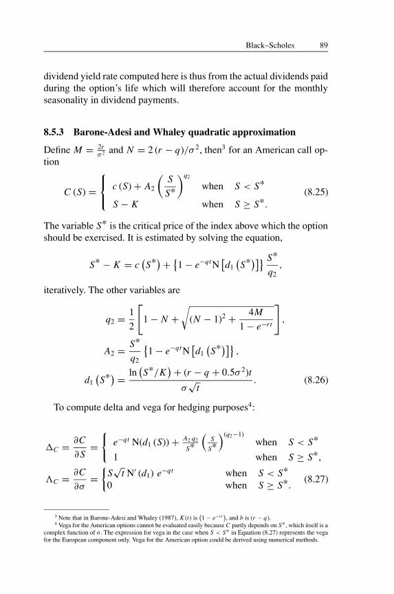
JWBK021-08 JWBK021-Poon March 14, 2005 23:18 Char Count= 0
Black–Scholes 89
dividend yield rate computed here is thus from the actual dividends paidduring the option’s life which will therefore account for the monthlyseasonality in dividend payments.
8.5.3 Barone-Adesi and Whaley quadratic approximation
Define M = 2rσ 2 and N = 2 (r − q)/σ 2, then3 for an American call op-
tion
C (S) = c (S) + A2
(S
S*
)q2
when S < S*
S − K when S ≥ S*.(8.25)
The variable S* is the critical price of the index above which the optionshould be exercised. It is estimated by solving the equation,
S* − K = c(S*
) + {1 − e−qt N
[d1
(S*
)]} S*
q2,
iteratively. The other variables are
q2 = 1
2
[1 − N +
√(N − 1)2 + 4M
1 − e−r t
],
A2 = S*
q2
{1 − e−qt N
[d1
(S*
)]},
d1(S*
) = ln(S*/K
) + (r − q + 0.5σ 2)t
σ√
t. (8.26)
To compute delta and vega for hedging purposes4:
�C = ∂C
∂S=
{e−qt N(d1 (S)) + A2 q2
S*
(S
S*
)(q2−1)when S < S*
1 when S ≥ S*,
�C = ∂C
∂σ=
{S√
t N′ (d1) e−qt when S < S*0 when S ≥ S*.
(8.27)
3 Note that in Barone-Adesi and Whaley (1987), K (t) is(1 − e−r t
), and b is (r − q).
4 Vega for the American options cannot be evaluated easily because C partly depends on S*, which itself is acomplex function of σ. The expression for vega in the case when S < S* in Equation (8.27) represents the vegafor the European component only. Vega for the American option could be derived using numerical methods.

JWBK021-08 JWBK021-Poon March 14, 2005 23:18 Char Count= 0
90 Forecasting Financial Market Volatility
For an American put option, the valuation formula is:
P (S) ={
p (S) + A1
(S
S**
)q1
when S > S**
K − S when S ≤ S**.(8.27a)
The variable S** is the critical index price below which the option shouldbe exercised. It is estimated by solving the equation,
K − S** = p(S**
) − {1 − e−qt N
[−d1(S**
)]} S**
q1,
iteratively. The other variables are
q1 = 1
2
[1 − N −
√(N − 1)2 + 4M
1 − e−r t
],
A1 = − S**
q1
{1 − e−qt N
[−d1(S**
)]},
d1(S**
) = ln(S**/K
) + (r − q + 0.5σ 2)t
σ√
t.
To compute delta and vega for hedging purposes:
�P = ∂ P
∂S=−e−qt N (d1 (S)) + A1 q1
S**
(S
S**
)(q1−1)
when S > S**
−1 when S ≤ S**,
�P = ∂ P
∂σ=
{∂C
∂σ= S
√t N′ (d1) e−qt when S > S**
0 when S ≤ S**.
8.6 MEASUREMENT ERRORS AND BIAS
Early studies of option implied volatility suffered many estimation prob-lems,5 such as the improper use of the Black–Scholes model for anAmerican style option, the omission of dividend payments, the optionprice and the underlying asset prices not being recorded at the sametime, or stale prices being used. Since transactions may take place at bidor ask prices, transaction prices of the option and the underlying assetsare subject to bid–ask bounce making the implied volatility estimation
5 Mayhew (1995) gives a detailed discussion on such complications involved in estimating implied volatilityfrom option prices, and Hentschel (2001) provides a discussion of the confidence intervals for implied volatilityestimates.

JWBK021-08 JWBK021-Poon March 14, 2005 23:18 Char Count= 0
Black–Scholes 91
unstable. Finally, in the case of an S&P100 OEX option, the privilegeof a wildcard option is often omitted.6 In more recent studies, many ofthese measurement errors have been taken into account. Many studiesuse futures and options futures because these markets are more activethan the cash markets and hence there is a smaller risk of prices beingstale.
Conditions in the Black–Scholes model include: no arbitrage, trans-action cost is zero and continuous trading. As mentioned before, thelack of such a trading environment will result in options being tradedwithin a band around the theoretical price. This means that impliedvolatility estimates extracted from market option prices will also liewithin a band even without the complications described in Chapter 10.Figlewski (1997) shows that implied volatility estimates can differ byseveral percentage points due to bid–ask spread and discrete tick sizealone. To smooth out errors caused by bid–ask bounce, Harvey and Wha-ley (1992) use a nonlinear regression of ATM option prices, observed ina 10-minute interval before the market close, on model prices.
Indication of nonideal trading environment is usually reflected in poortrading volume. This means implied volatility of options written ondifferent underlying assets will have different forecasting power. Formost option contracts, ATM option has the largest trading volume. Thissupports the popularity of ATM implied volatility referred to later inChapter 10.
8.6.1 Investor risk preference
In the Black–Scholes world, investor risk preference is irrelevant inpricing options. Given that some of the Black–Scholes assumptions havebeen shown to be invalid, there is now a model risk. Figlewski andGreen (1999) simulate option writers positions in the S&P500, DM/$,US LIBOR and T-Bond markets using actual cash data over a 25-yearperiod. The most striking result from the simulations is that delta hedgedshort maturity options, with no transaction costs and a perfect knowledgeof realized volatility, finished with losses on average in all four markets.This is clear evidence of Black–Scholes model risk. If option writersare aware of this model risk and mark up option prices accordingly, theBlack–Scholes implied volatility will be greater than the true volatility.
6 This wildcard option arises because the stock market closes later than the option market. The option traderis given the choice to decide, before the stock market closes, whether or not to trade on an option whose price isfixed at an earlier closing time.

JWBK021-08 JWBK021-Poon March 14, 2005 23:18 Char Count= 0
92 Forecasting Financial Market Volatility
In some situations, investor risk preference may override the risk-neutral valuation relationship. Figlewski (1997), for example, comparesthe purchase of an OTM option to buying a lottery ticket. Investors arewilling to pay a price that is higher than the fair price because they likethe potential payoff and the option premium is so low that mispricingbecomes negligible. On the other hand, we also have fund managers whoare willing to buy comparatively expensive put options for fear of thecollapse of their portfolio value. Both types of behaviour could causethe market price of options to be higher than the Black–Scholes price,translating into a higher Black–Scholes implied volatility. Arbitrage ar-guments do not apply here because these are unique risk preferences(or aversions) associated with some groups of individuals. Franke, Sta-pleton and Subrahmanyam (1998) provide a theoretical framework inwhich such option trading behaviour may be analysed.
8.7 APPENDIX: IMPLEMENTING BARONE-ADESIAND WHALEY’S EFFICIENT ALGORITHM
The determination of S* and S** in Equations (8.25) and (8.27a) arenot exactly straightforward. We have some success in solving S* andS** using NAG routing C05NCF. Barone-Adesi and Whaley (1987),however, have proposed an efficient method for determining S*, detailsof which can be found in Barone-Adesi and Whaley (1987, hereafterreferred to as BAW) pp. 309 to 310. BAW claimed that convergence ofS* and S** can be achieved with three or fewer iterations.
American calls
The following are step-by-step procedures for implementing BAW’sefficient method for estimating S∗ of the American call.
Step 1. Make initial guess of σ and denote this initial guess as σ j withj = 1.
Step 2. Make initial guess of S*, Si (with i = 1), as follow; denotingS* at T = +∞ as S* (∞) :
S1 = X + [S* (∞) − K
] [1 − eh2
], (8.28)
where
S* (∞) = K
1 − 1
q2 (∞)
, (8.29)

JWBK021-08 JWBK021-Poon March 14, 2005 23:18 Char Count= 0
Black–Scholes 93
q2 (∞) = 1
2
[1 − N +
√(N − 1)2 + 4M
], (8.30)
h2 = −(
(r − q) t + 2σ√
t){
K
S* (∞) − K
}. (8.31)
Note that the lower bound of S* is K . So if S1 < K , resetS1 = K . However, the condition S* < K rarely occurs.
Step 3. Compute the l.h.s. and r.h.s. of Equation (8.25a) as follows:
l.h.s. (Si ) = Si − X, and (8.32)
r.h.s. (Si ) = c (Si ) + {1 − e−qt N [d1 (Si )]
}Si/q2. (8.33)
Compute starting value of c (Si ) using the simple Black–ScholesEquation (8.25) and d1 (Si ) using Equation (8.26). It will beuseful to set up a function (or subroutine variable) for d1.
Step 4. Check tolerance level,
|l.h.s. (Si ) − r.h.s. (Si )| /K < 0.000 01. (8.34)
Step 5. If Equation (8.34) is not satisfied; compute the slope of Equation(8.33), bi , and the next guess of S*, Si+1, as follows:
bi = e−qt N [d1 (Si )] (1 − 1/q2)
+[1 − e−qt n[d1 (Si )]/σ
√t]/q2, (8.35)
Si+1 = [X + r.h.s. (Si ) − bi Si ] / (1 − bi ) , (8.36)
where n (.) is the univariate normal density function. Repeatfrom step 3.
Step 6. When Equation (8.34) is satisfied, compute C (S) according toEquation (8.25). If C (S) is greater than the observed Americancall price, try a smaller σ j+1, otherwise try a larger σ j+1. Repeatsteps 1 to 5 until C (S) is the same as the observed Americancall price. Step 6 could be handled by a NAG routine such asC05ADF for a quick solution.
American puts
To approximate S** for American puts, steps 2, 3 and 5 have to bemodified.
Step 1. Make initial guess of σ and denote this initial guess as σ j withj = 1.

JWBK021-08 JWBK021-Poon March 14, 2005 23:18 Char Count= 0
94 Forecasting Financial Market Volatility
Step 2. Make initial guess of S**, Si (with i = 1), as follows, denotingS** at T = +∞ as S** (∞):
S1 = S** (∞) + [K − S** (∞)
]eh1, (8.37)
where
S** (∞) = K
1 − 1
q1 (∞)
,
q1 (∞) = 1
2
[1 − N −
√(N − 1)2 + 4M
],
h1 =(
(r − q) t − 2σ√
t){
K
K − S** (∞)
}. (8.38)
Note that the upper bound of S** is K . So if S1 > K , resetS1 = K . Again, the condition S** > X rarely occurs. Accord-ing to Barone-Adesi and Whaley (1987, footnote 9), the influ-ence of (r − q) must be bounded in the put exponent to ensurecritical prices monotonically decrease in t , for very large val-ues of (r − q) and t . A reasonable bound on (r − q) is 0.6σ
√t ,
so the critical stock price declines with a minimum velocitye−1.4σ
√t . This check is required before computing h1, in Equa-
tion (8.38).Step 3. Compute the l.h.s. and r.h.s. of Equation (8.37) as follows:
l.h.s. (Si ) = K − Si , and
r.h.s. (Si ) = p (Si ) − {1 − e−qt N [−d1 (Si )]
}Si/q1. (8.39)
Step 4. Check tolerance level, as before,
|l.h.s. (Si ) − r.h.s. (Si )| /K < 0.00001. (8.40)
Step 5. If Equation (8.40) is not satisfied; compute the slope of Equation(8.39), bi , and the next guess of S**, Si+1, as follows:
bi = −e−qt N [−d1 (Si )] (1 − 1/q1)
−[1 + e−qt n [d1 (Si )] /σ
√t]/q1,
Si+1 = [X − r.h.s. (Si ) + bi Si ] / (1 + bi ) .
Repeat from step 3 above.

JWBK021-08 JWBK021-Poon March 14, 2005 23:18 Char Count= 0
Black–Scholes 95
Step 6. When Equation (8.40) is satisfied, compute P (S) using Equa-tion (8.27a). If P (S) is greater than the observed American callprice, try a larger σ j+1, otherwise try a smaller σ j+1. Then repeatsteps 1 to 5 until P (S) is the same as the observed American putprice. Similarly the case for the American call, step 6 could behandled by a NAG routine such as C05ADF for a quick solution.

JWBK021-09 JWBK021-Poon March 14, 2005 23:19 Char Count= 0
9Option Pricing with Stochastic
Volatility
If Black–Scholes (BS) is the correct option pricing model, then therecan only be one BS implied volatility regardless of the strike price ofthe option, or whether the option is a call or a put. BS implied volatilitysmile and skew are clear evidence that market option prices are not pricedaccording to the BS formula. This raises the important question aboutthe relationship between BS implied volatility and the true volatility.
The BS option price is a positive function of the volatility of theunderlying asset. If the BS model is correct, then market option priceshould be the same as the BS option price and the BS implied volatilityderived from market option price will be the same as the true volatility.If the BS price is incorrect and is lower than the market price, then BSimplied volatility overstates the true volatility. The reverse is true if theBS price is higher than the market price. The problem is complicatedby the fact that BS implied volatility differs across strike prices. All thetheories that predict the relationship between BS price and the marketoption price are all contingent on the proposed alternative option pricingmodel or the proposed alternative pricing dynamic being correct. Giventhat the BS implied volatility, despite all its shortcomings, has beenproven overwhelmingly to be the best forecast of volatility, it will beuseful to understand the links between BS implied volatility bias andthe true volatility. This is the objective of this chapter.
There have been a lot of efforts made to solve the BS anomalies.The stochastic volatility (SV) option pricing model is one of the mostimportant extensions of Black–Scholes. The SV option pricing modelis motivated by the widespread evidence that volatility is stochastic andthat the distribution of risky asset returns has tail(s) longer than that ofa normal distribution. An SV model with correlated price and volatilityinnovations can address both anomalies. The SV option pricing modelwas developed roughly over a decade with contributions from Johnsonand Shanno (1987), Wiggins (1987), Hull and White (1987, 1988), Scott(1987), Stein and Stein (1991) and Heston (1993). It was in Heston(1993) that a closed form solution was derived using the characteristic
97

JWBK021-09 JWBK021-Poon March 14, 2005 23:19 Char Count= 0
98 Forecasting Financial Market Volatility
function of the price distribution. Section 9.1 presents this landmarkHeston SV option pricing model while some details of the derivation arepresented in the Appendix to this chapter (Section 9.5). In Section 9.2,we simulate a series of Heston option prices from a range of parameters.Then we use these option prices as if they were the market option pricesto back out the corresponding BS implied volatilities. If market optionprices are priced according to the Heston formula, the simulations inthis section will give us some insight into the relationship between BSimplied volatility bias and the true volatility. In Section 9.3, we analysethe usefulness and practicality of the Heston model by looking at theimpact of Heston model parameters on skewness and kurtosis range andsensitivity, and some empirical tests of Heston model. Finally, Section9.4 analyses empirical findings on the the predictive power of Hestonimplied volatility as a volatility forecast.
9.1 THE HESTON STOCHASTIC VOLATILITYOPTION PRICING MODEL
Heston (1993) specifies the stock price and volatility price processes asfollows:
d St = µSdt + √υt Sdzs,t ,
dυt = κ [θ − υt ] dt + σν
√υt dzυ,t ,
where υt is the instantaneous variance, κ is the speed of mean reversion,θ is the long-run level of volatility and σν is the ‘volatility of volatility’.The two Wiener processes, dzs,t and dzυ,t have constant correlation ρ.The assumption that consumption growth has a constant correlation withspot-asset returns generates a risk premium proportional to υt . Given thevolatility risk premium, the risk-neutral volatility process can be writtenas
dυt = κ [θ − υt ] dt − λυt dt + σν
√υt dz*
υ,t
= κ*[θ* − υt
]dt + σν
√υt dz*
υ,t ,
where λ is the market price of (volatility) risk, and κ* = κ + λ andθ* = κθ/(κ + λ). Here κ* is the risk-neutral mean reverting parameterand θ* is the risk-neutral long-run level of volatility. The parameter σν
and ρ implicit in the risk-neutral process are the same as that in thereal volatility process. Given the price and the volatility dynamics, the

JWBK021-09 JWBK021-Poon March 14, 2005 23:19 Char Count= 0
Option Pricing with Stochastic Volatility 99
Heston (1993) formula for pricing European calls is
c = S P1 − K e−r (T −t) P2,
Pj = 1
2+ 1
π
∫ ∞
0Re
[e−iφ ln K fi
iφ
]dφ, for j = 1, 2
fi = exp {C (T − t ; φ) + D (T − t ; φ) υ + iφx} ,
where
x = ln S, τ = T − t,
C (τ ; φ) = rφiτ + a
σ 2ν
{(b j − ρσνφi + d
)τ − 2 ln
[1 − gedτ
1 − g
]},
D (τ ; φ) = b j − ρσνφi + d
σ 2ν
[1 − edτ
1 − gedτ
],
g = b j − ρσνφi + d
b j − ρσνφi − d,
d =√(
ρσνφi − b j)2 − σ 2
ν
(2µφi − φ2
),
µ1 = 1/
2 , µ2 = −1/
2 , a = κθ = κ*θ*,
b1 = κ + λ − ρσν = κ* − ρσν, b2 = κ + λ = κ*.
9.2 HESTON PRICE AND BLACK–SCHOLES IMPLIED
In this section, we analyse possible BS implied bias by simulating aseries of Heston option prices with parameter values similar to those inBakshi, Cao and Chen (1997), Nandi (1998), Das and Sundaram (1999),Bates (2000), Lin, Strong and Xu (2001), Fiorentini, Angel and Rubio(2002) and Andersen, Benzoni and Lund (2002). For the simulations, weset the asset price as 100, interest rate as zero, time to maturity is 1 year,and strike prices ranging from 50 to 150. In most simulations, and unlessotherwise stated, the current ‘instantaneous’ volatility, σt , is set equal tothe long-run level, θ , at 20%. There are five other parameters used in theHeston formula, namely, κ , the speed of mean reversion, θ , the long-runvolatility level, λ, the market price of risk, συ , volatility of volatility, andρ, the correlation between the price and the volatility processes. If weset λ = 0, then the volatility process becomes risk-neutral, and κ and θ
become κ* and θ* respectively.The first set of simulations presented in Figure 9.1(a) involves repli-
cating the Black–Scholes prices as a special case. Here we set συ = 0.

JWBK021-09 JWBK021-Poon March 14, 2005 23:19 Char Count= 0
100 Forecasting Financial Market Volatility
(e) Effect of l on negatively correlated processes (S = 100, r = 0, T = 1, r = -0.5)
Skewness = +0.1623, Kurtosis = 3.7494
0
0.05
0.1
0.15
0.2
0.25
0.3
0.35
0.4
0.45
50 60 70 80 90 100 110 120 130 140 150
Strike Price, K
BS
Im
plie
d
l = -2 l = 0 l = 2
(f) Effect of l on positively correlated processes (S = 100, r = 0, T = 1, r = 0.5)
Skewness = -0.1623, Kurtosis = 3.7494
0
0.05
0.1
0.15
0.2
0.25
0.3
0.35
0.4
0.45
50 60 70 80 90 100 110 120 130 140 150
Strike Price, K
BS
Im
plie
d
l = -2 l = 0 l = 2
(c) Effect of correlation, r
0
0.05
0.1
0.15
0.2
0.25
0.3
0.35
0.4
50 60 70 80 90 100 110 120 130 140 150
Strike Price, K
BS
Im
plie
d
r = -0.95 r = -0.5
r = 0 r = 0.6
(d) Effect of k(S = 100, r = 0, T = 1, l = 0, su = 0.6, q = 0.2)
0.10490
0.1
0.2
0.3
0.4
0.5
0.6
0.7
0.8
50 60 70 80 90 100 110 120 130 140 150
Strike Price, K
BS
Im
plie
dk = 0.01, √υt = 0.7 k = 3, √υt = 0.7
k = 0.01, √υt = 0.15 k = 3, √υt = 0.15
(a) A Black–Scholes series(S = 100, r = 0, T = 1, l = 0)
(S = 100, r = 0, T = 1, l = 0)
Skewness = 0, Kurtosis = 3
0
0.05
0.1
0.15
0.2
0.25
0.3
0.35
0.4
0.45
50 60 70 80 90 100 110 120 130 140 150
Strike Price, K
BS
Im
plie
d(b) Effect of volatility of volatility (su, Kurtosis)
(S = 100, r = 0, T = 1, l = 0, k = 0.1)
0
0.05
0.1
0.15
0.2
0.25
0.3
0.35
0.4
0.45
50 60 70 80 90 100 110 120 130 140 150
Strike Price, K
BS
Im
plie
d
su = 0.1 , Kur = 3.7
su = 0.3, Kur = 9.53
su = 0.6, Kur = 29.1
su = 1.0, Kur = 75.6
Figure 9.1 Relationships between Heston option prices and Black–Scholes impliedvolatility
Since there is no volatility risk, λ = 0. This is a special case wherethe Heston price and the Black–Scholes price are identical and the BSimplied volatility is the same across strike prices. In this special case,BS implied volatility (at any strike price) is a perfect representation oftrue volatility.

JWBK021-09 JWBK021-Poon March 14, 2005 23:19 Char Count= 0
Option Pricing with Stochastic Volatility 101
In the second set of simulations presented in Figure 9.1(b), we al-ter συ , the volatility of volatility, and keep all the other parameters thesame and constant. The effect of an increase in συ is to increase theunconditional volatility and kurtosis of risk-neutral price distribution. Itis the risk-neutral distribution because λ, the market price of risk, is setequal to zero. As συ increases and without appropriate compensation forvolatility risk premium, ATM (at-the-money) implied volatility under-estimates true volatility while OTM (out-of-the-money) implied volatil-ity overestimates it. This is the same outcome as Hull and White (1987)where the price and the volatility processes are not correlated and thereis no risk premium for volatility risk. With appropriate adjustment forvolatility (which will require a volatility risk premium input), the ATMimplied volatility will be at the right level, but Black–Scholes will con-tinue to underprice OTM options (and OTM BS implied overestimatestrue volatility) because of the BS lognormal thin tail assumptions. As-suming that ρ = 0 or at least is constant over time, and that συ and λ arerelatively stable, a time series regression of historical ‘actual volatility’on historical ‘implied volatility’ at a particular strike will be sufficientto correct for these biases. This is basically the Ederington and Guan(1999) approach. We will show in the next section that ρ is not likely tobe stable. When ρ is not constant, the analysis below and Figure 9.1(c)show that ATM implied volatility is least affected by changing ρ. Thisexplains why ATM implied volatility is the most robust and popularchoice of volatility forecast.
In Figure 9.1(c), it is clear that changing the correlation coefficientalone has no impact on ATM implied volatility. Correlation has thegreatest impact on skewness of the price distribution and determines theshape of volatility smile or skew. Its impact on kurtosis is less markedwhen compared with συ , the volatility of volatility.
Figure 9.1(d) highlights the impact of κ , the mean reversion parameterwhich we have already briefly touched on in relation to the long memoryof volatility in Chapter 5. The higher the rate of mean reversion, the morelikely the return distribution will be normal even when the volatility ofvolatility, συ , and the initial volatility,
√νt , are both high. When this is
the case, there is no strike price bias in BS implied (i.e. there will not bevolatility smile). When κ is low, this is when the problem starts. A low κ
corresponds with volatility persistence where BS implied volatility willbe sensitive to the current state of volatility level. At high volatility state,high
√νt compensates for the lowκ and the strike price bias is less severe.
Strike price effect or the volatility smile is the most acute when initialvolatility level
√νt is low. ATM options will be overpriced vis-a-vis

JWBK021-09 JWBK021-Poon March 14, 2005 23:19 Char Count= 0
102 Forecasting Financial Market Volatility
OTM options.1 (Note that we have set λ = 0 in this set of simulations.)When συ = 0.6, θ = 0.2,
√νt = 0.15 and κ = 0.01, the ATM BS im-
plied is only 0.1049 much lower than any of the volatility parameters.Figure 9.1(e) and 9.1(f) can be used to infer the impacts of parameter
estimates above when the volatility risk premium λ is omitted. In theliterature, we often read ‘. . . volatility risk premium is negative reflect-ing the negative correlation between the price and the volatility dyna-mics . . . ’ (Buraschi and Jackwerth, 2001; Bakshi and Kapadia, 2003.All series in Figure 9.1(e) have correlation ρ = −0.5 and all series inFigure 9.1(f) have correlation ρ = +0.5. A negative λ (volatility riskpremium) produces higher Heston price and higher BS implied volatil-ity. The impact is the same whether the correlation ρ is negative orpositive. We will see later in the next section that empirical evidence in-dicates that Figure 9.1(f) is just as likely a scenario as Figure 9.1(e). Asκ* = κ + λ and θ* = κθ/(κ + λ), a negative λ has the effect of reduc-ing κ* (resulting in a smaller option price) and increasing θ* (resultingin a bigger option price). Simulations, not reported here, show that theprice impact of θ* is much greater than that of κ*, so the outcome willbe a higher option price due to the negative λ. Hence, a ‘negative riskpremium’ is to be expected whether the price and the volatility processesare positively or negatively correlated.2 This also means that, withoutaccounting for the volatility risk premium, the BS option price will betoo low and the BS implied will always overstate true volatility. Bothvolatility and volatility risk premium have positive impact on optionprice. The omission of volatility risk premium will cause the volatil-ity risk premium component to be ‘translated’ into higher BS impliedvolatility.
9.3 MODEL ASSESSMENT
In this section, we evaluate the Heston model using simulations. In par-ticular, we examine the skewness and kurtosis planes covered by a rangeof Heston parameter values. We have no information on the volatilityrisk premium. Hence, to avoid an additional dimension of complexity,we will evaluate the risk-neutral parameters κ* and θ* instead of κ andθ for the true volatility process.
1 When BS overprice options, the BS implied volatility will understate volatility because BS implied isinverted from market price, which is lower than the BS price.
2 This is really a misnomer: while the λ parameter is negative, it actually results in a higher option price. Sostrictly speaking the volatility risk premium is positive!

JWBK021-09 JWBK021-Poon March 14, 2005 23:19 Char Count= 0
Option Pricing with Stochastic Volatility 103
9.3.1 Zero correlation
We learn from the simulations in Section 9.2 and from Figure 9.1 that,according to the Heston model, skewness in stock returns distributionand BS implied volatility asymmetry are determined completely by thecorrelation parameter, ρ. When the correlation parameter is equal tozero, we get zero skewness and both the returns distribution and BSimplied volatility will be symmetrical. Figure 9.2 presents the kurtosisvalues produced by different combinations of κ , θ and σv. One importantpattern emerged that highlights the importance of the mean reversionparameter, κ . When κ is low we have high volatility persistence, andvice versa for high value of κ .
At high value of κ , kurtosis is close to 3, regardless of the value of θ andσv. This is, unfortunately, the less likely scenario for a financial markettime series that typically has high volatility persistence and low valueof κ . At low value of κ , the kurtosis is the highest at low level of σv, theparameter for volatility of volatility. At high level of σv, kurtosis dropsto 3 very consistently, regardless of the value of the other parameters.At low level of σv, the long-term level of volatility, θ , comes into effect.The higher the value of θ , the lower the kurtosis value, even though it isstill much greater than 3.
When skewness is zero and kurtosis is low (i.e. relatively flat BS im-plied volatility), it will be difficult to differentiate whether it is due toa high κ , a high σv or both. This also reflects the underlying prop-erty that a high κ , a high σv or both make the stochastic volatilitystructure less important and the BS model will be adequate in thiscase.
9.3.2 Nonzero correlation
In Figures 9.3 and 9.4, we illustrate skewness and kurtosis, respectively,for the case when the correlation coefficient, ρ, is greater than 0. Thecase for ρ < 0 will not be discussed here as it is the reflective imageof ρ > 0 (e.g. instead of positive skewness, we get negative skewnessetc.).
Figure 9.3 shows that skewness is first ‘triggered’ by a nonzero cor-relation coefficient, after which κ and σv combine to drive skewness.High skewness occurs when σv is high and κ is low (i.e. high volatilitypersistence). At relatively low skewness level, there is a huge range ofhigh κ , low σv or both that produce similar values of skewness. A low θ

JWBK021-09 JWBK021-Poon March 14, 2005 23:19 Char Count= 0
104 Forecasting Financial Market Volatility
0.05 0.1 0.15 0.2 0.25 0.3 0.1 0.2 0.3 0.4 0.5
0
10
20
30
40
50
60
70
80
Kurtosis
q
(a) k = 1, r = 0, Skewness = 0
0.10.2
0.30.4
0.5
0.10.2
0.30.4
0.5
0.00
10.00
20.00
30.00
40.00
50.00
60.00
70.00
80.00
Kurtosis
su q
(b) k = 0.1, r = 0, Skewness = 0
su
Figure 9.2 Impact of Heston parameters on kurtosis for symmetrical distribution withzero correlation and zero skewness
and high ρ produces high skewness, but at low level of σv, skewness ismuch less sensitive to these two parameters.
Figure 9.4 gives a similar pattern for kurtosis. Except when σv is veryhigh and κ is low, the plane for kurtosis is very flat and not sensitive toθ or ρ.

JWBK021-09 JWBK021-Poon March 14, 2005 23:19 Char Count= 0
Option Pricing with Stochastic Volatility 1050.
05
0.2
0.1 0.
3 0.5 0.7 0.9
0
0.5
1
1.5
2
2.5
3
3.5
Skewness
q r
k = 1, su = 0.5
0.05
0.2
0.1 0.
3 0.5 0.7 0.9
0
0.5
1
1.5
2
2.5
3
3.5
Skewness
q r
k = 1, su = 0.1
0.05
0.2
0.1 0.
3 0.5 0.7 0.9
0
0.5
1
1.5
2
2.5
3
3.5
Skewness
q r
k = 0.1, su = 0.5
0.05
0.2
0.1 0.
3 0.5 0.7 0.9
0
0.5
1
1.5
2
2.5
3
3.5
Skewness
q r
k = 0.1, su = 0.1
Figure 9.3 Impact of Heston parameters on skewness
9.4 VOLATILITY FORECAST USING THEHESTON MODEL
The thick tail and nonsymmetrical distribution found empirically couldbe a result of volatility being stochastic. The simulation results in theprevious section suggest that σv, the volatility of volatility, is the maindriving force for kurtosis and skewness (if correlation is not equal tozero). At high κ , volatility mean reversion will cancel out much ofthe σv impact on kurtosis and some of that on skewness. Correlationbetween the price and the volatility processes, ρ, determines the sign ofthe skewness. But beyond that its impact on the magnitude of skewnessis much less compared with σv and κ . Correlation has negligible impacton kurtosis. The long-run volatility level, θ , has very little impact onskewness and kurtosis, except when σv is very high and κ is very low. Soa stochastic volatility pricing model is useful and will outperform Black–Scholes only when volatility is truly stochastic (i.e. high σv) and volatilityis persistent (i.e. lowκ). The difficulty with the Heston model is that, once

JWBK021-09 JWBK021-Poon March 14, 2005 23:19 Char Count= 0
106 Forecasting Financial Market Volatility
0.05
0.2
0.1 0.
3 0.5 0.7 0.9
0102030405060708090
Kurtosis
q r
k = 1, su = 0.50.
05
0.2
0.1 0.
3 0.5 0.7 0.9
0102030405060708090
Kurtosis
q r
k = 1, su = 0.10.
05
0.2
0.1 0.
3 0.5 0.7 0.9
0102030405060708090
Kurtosis
q r
k = 0.1, su = 0.5
0.05
0.2
0.1 0.
3 0.5 0.7 0.9
0102030405060708090
Kurtosis
q r
k = 0.1, su = 0.1
Figure 9.4 Impact of Heston parameters on kurtosis
we move away from the high σv and low κ region, a large combinationof parameter values can produce similar skewness and kurtosis. Thiscontributes to model parameter instability and convergence difficultyduring estimation.
Through simulation results we can predict the degree of Black–Scholes pricing bias as a result of stochastic volatility. In the case wherevolatility is stochastic and ρ = 0, Black–Scholes overprices near-the-money (NTM) or at-the-money (ATM) options and the degree of over-pricing increases with maturity. On the other hand, Black–Scholes un-derprices both in- and out-of-the-money options. In term of impliedvolatility, ATM implied volatility will be lower than actual volatilitywhile implied volatility of far-from-the-money options (i.e. either veryhigh or very low strikes) will be higher than actual volatility. The patternof pricing bias will be much harder to predict if ρ is not zero, when thereis a premium for bearing volatility risk, and if either or both values varythrough time.

JWBK021-09 JWBK021-Poon March 14, 2005 23:19 Char Count= 0
Option Pricing with Stochastic Volatility 107
Some of the early work on option implied volatility focuses on find-ing an optimal weighting scheme to aggregate implied volatility of op-tions across strikes. (See Bates (1996) for a comprehensive survey ofthese weighting schemes.) Since the plot of implied volatility againststrikes can take many shapes, it is not likely that a single weightingscheme will remove all pricing errors consistently. For this reason andtogether with the liquidity argument, ATM option implied volatility isoften used for volatility forecast but not implied volatilities at otherstrikes.
9.5 APPENDIX: THE MARKET PRICE OFVOLATILITY RISK
9.5.1 Ito’s lemma for two stochastic variables
Given two stochastic processes,3
d S1 = µ1 (S1, S2, t) dt + σ1 (S1, S2, t) d X1,
d S2 = µ2 (S1, S2, t) dt + σ2 (S1, S2, t) d X2,
E {d X1d X2} = ρdt,
where X1 and X2 are two related Brownian motions.From Ito’s lemma, the derivative function V (S1, S2, t) will have the
following process:
dV ={
Vt + 1
2σ 2
1 VS1 S1 + ρσ1σ2VS1 S2 + 1
2σ 2
2 VS2 S2
}dt
+VS1d S1 + VS2d S2,
where
Vt = ∂V
∂t, VS1 S1 = ∂2V
∂S21
and VS1 S2 = ∂
∂S1
(∂V
∂S2
).
9.5.2 The case of stochastic volatility
Here, we assume S1 is the underlying asset and S2 is the stochasticvolatility σ1 as follows:
d S1 = µ1 (S1, σ, t) dt + σ1 (S1, σ, t) d X1, (9.1)
dσ1 = p (S1, σ, t) dt + q (S1, σ, t) d X2,
E {d X1d X2} = ρdt,
3 I am grateful to Konstantinos Vonatsos for helping me with materials presented in this section.

JWBK021-09 JWBK021-Poon March 14, 2005 23:19 Char Count= 0
108 Forecasting Financial Market Volatility
and from Ito’s lemma, we get:
dV ={
Vt + 1
2σ 2
1 VS1 S1 + ρqσ1VS1σ + 1
2q2VS2σ
}dt (9.2)
+VS1d S1 + Vσ dσ.
In the following stochastic volatility derivation, µ1 = µSt is the meandrift of the stock price process. The volatility of S1, σ1 = f (σ ) S1 isstochastic and is level-dependent. The mean drift of the volatility pro-cess is more complex as volatility cannot become negative and shouldbe stationary in the long run. Hence an OU (Ornstein–Uhlenbeck)process is usually recommended with p (S1, σ, t) = α (m − σ ) andq (S1, σ, t) = β:
dσ1 = α (m − σ1) dt + βd X2.
Here, p = α (m − σ ) is the mean drift of the volatility process, m isthe long-term mean level of the volatility, and α is the speed at whichvolatility reverts to m, and β is the volatility of volatility.
9.5.3 Constructing the risk-free strategy
To value an option V (S1, σ, t) we must form a risk-free portfolio usingthe underlying asset to hedge the movement in S1 and use another optionV (S1, σ, t) to hedge the movement in σ . Let the risk-free portfolio be:
� = V − �1V − �S1.
Applying Ito’s lemma from (9.2) on the risk-free portfolio �,
d� ={
Vt + 1
2σ 2
1 VS1 S1 + 1
2q2Vσσ + ρqσ1VS1σ
}dt
−�1
{V t + 1
2σ 2
1 V S1 S1 + 1
2q2V σσ + ρqσ1V S1σ
}dt
+ {VS1 − �1V S1 − �
}d S1
+ {Vσ − �1V σ
}dσ.
To eliminate dσ , set
Vσ − �1V σ = 0,
�1 = Vσ
V σ
,

JWBK021-09 JWBK021-Poon March 14, 2005 23:19 Char Count= 0
Option Pricing with Stochastic Volatility 109
and, to eliminate d S1, set
VS1 − Vσ
V σ
V S1 − � = 0,
� = VS1 − Vσ
V σ
V S1 .
This results in:
d� ={
Vt + 1
2σ 2
1 VS1 S1 + 1
2q2Vσσ + ρqσ1VS1σ
}dt
− Vσ
V σ
{V t + 1
2σ1
2V S1 S1 + 1
2q2V σσ + ρqσ1V S1σ
}dt
= r�dt
= r
{V − Vσ
V σ
V −[
VS1 − Vσ
V σ
V S1
]S1
}dt.
Dividing both sides by Vσ , we get:
1
Vσ
{Vt + 1
2σ 2
1 VS1 S1 + 1
2q2Vσσ + ρqσ1VS1σ
}− 1
V σ
{V t + 1
2σ 2
1 V S1 S1 + 1
2q2V σσ + ρqσ1V S1σ
}= r
V
Vσ
− rV
V σ
− rVS1 S1
Vσ
+ rV S1 S1
V σ
.
Now we separate the two options by moving V to one side and V to theother:
1
Vσ
{Vt + 1
2σ 2
1 VS1 S1 + 1
2q2Vσσ + ρqσ1VS1σ − r V + r VS1 S1
}= 1
V σ
{V t + 1
2σ 2
1 V S1 S1 + 1
2q2V σσ + ρqσ1V S1σ − r V + r V S1 S1
}.
Each side of the equation is a function of S1, σ and t , and is independentof the other option. So we may write:
1
Vσ
{Vt + 1
2σ 2
1 VS1 S1 + 1
2q2Vσσ + ρqσ1VS1σ − r V + r VS1 S1
}= f (S1, σ, t) ,
Vt + 1
2σ 2
1 VS1 S1 + 1
2q2Vσσ + ρqσ1VS1σ − r V + r VS1 S1
= f (S1, σ, t) Vσ , (9.3)

JWBK021-09 JWBK021-Poon March 14, 2005 23:19 Char Count= 0
110 Forecasting Financial Market Volatility
and similarly for the RHS. In order to solve the PDE, we need to under-stand the function f (S1, σ, t) which depends on whether or not d S1 anddσ are correlated.
9.5.4 Correlated processes
If two Brownian motions d X1 and d X2 are correlated with correlationcoefficient ρ, then we may write:
d X2 = ρd X1 +√
1 − ρ2dεt ,
where dεt is the part of d X2 that is not related to d X1.Now consider the hedged portfolio,
� = V − �S1, (9.4)
where only the risk that is due to the underlying asset and its correlatedvolatility risk are hedged. Volatility risk orthogonal to d S1 is not hedged.From Ito’s lemma, we get:
d� = dV − �d S1
={
Vt + 1
2σ 2
1 VS1 S1 + ρqσ1VS1σ + 1
2q2Vσσ
}dt
+VS1d S1 + Vσ dσ − �d S1. (9.5)
Now write:
d S1 = µ1dt + σ1d X1, and
dσ = pdt + qd X2
= pdt + q[ρd X1 +
√1 − ρ2dεt
].
Substitute this result into (9.5) and get:
d� ={
Vt + 1
2σ 2
1 VS1 S1 + ρqσ1VS1σ + 1
2q2Vσσ
}dt
+VS1 {µ1dt + σ1d X1} + Vσ
{pdt + q
[ρd X1 +
√1 − ρ2dεt
]}−� {µ1dt + σ1d X1}
={
Vt + 1
2σ 2
1 VS1 S1 + ρqσ1VS1σ + 1
2q2Vσσ
}dt
+ (VS1µ1 + Vσ p − �µ1
)dt + (
VS1σ1 + Vσ qρ − �σ1)
d X1
+Vσ q√
1 − ρ2dεt . (9.6)

JWBK021-09 JWBK021-Poon March 14, 2005 23:19 Char Count= 0
Option Pricing with Stochastic Volatility 111
So to get rid of d X1, the hedge ratio should be:
VS1σ1 + Vσ qρ − �σ1 = 0,
� = VS1 + Vσ qρ
σ1.
With this hedge ratio, only the uncorrelated volatility risk,Vσ q
√1 − ρ2dεt , is left in the portfolio. If ρ = 1, the portfolio � would
be risk-free.Now substitute value of � into (9.6). We get:
d� ={
Vt + 1
2σ 2
1 VS1 S1 + ρqσ1VS1σ + 1
2q2Vσσ
}dt
+(
VS1µ1 + Vσ p − VS1µ1 − Vσ qρµ1
σ1
)dt + Vσ q
√1 − ρ2dεt
={
Vt + 1
2σ 2
1 VS1 S1 + ρqσ1VS1σ + 1
2q2Vσσ
}dt
+(
Vσ p − Vσ qρµ1
σ1
)dt + Vσ q
√1 − ρ2dεt . (9.7)
9.5.5 The market price of risk
Next we made the assumption that the partially hedged portfolio � in(9.4) will earn a risk-free return plus a premium for unhedged volatilityrisk, �, such that
d� = r�dt + �
= r (V − �S1) dt + �
= r
(V − VS1 S1 − Vσ qρ
σ1S1
)dt + �. (9.8)
Substituting d� from (9.7), we get:{Vt + 1
2σ 2
1 VS1 S1 + ρqσ1VS1σ + 1
2q2Vσσ
}dt
+(
Vσ p − Vσ qρµ1
σ1
)dt + Vσ q
√1 − ρ2dεt
= r V dt − r VS1 S1dt − rVσ qρ
σ1S1dt + �,

JWBK021-09 JWBK021-Poon March 14, 2005 23:19 Char Count= 0
112 Forecasting Financial Market Volatility
� ={
Vt + 1
2σ 2
1 VS1 S1 + ρqσ1VS1σ + 1
2q2Vσσ − r V + r VS1 S1
}dt
+[
Vσ p + Vσ qρ
σ1(r S1 − µ1)
]dt + Vσ q
√1 − ρ2dεt .
Now replace the {} term with f (S1, σ, t) in (9.3) we get:
� =(
f Vσ + Vσ p + Vσ qρ
σ1(r S1 − µ1)
)dt + Vσ q
√1 − ρ2dεt
= Vσ q√
1 − ρ2
{[f + p + qρ
σ1(r S1 − µ1)
q√
1 − ρ2
]dt + dεt
}.
Now define ‘market price of risk’ γ :
γ =f + p + qρ
σ1(r S1 − µ1)
q√
1 − ρ2, (9.9)
where γ is the ‘returns’ associated with each unit of risk that is due to dεt
(i.e. the unhedged volatility risk), hence, the denominator q√
1 − ρ2.From (9.9), we can get an expression for f :
f = −p + qρ
σ1(µ1 − r S1) + γ q
√1 − ρ2.
Substituting p = α (m − σ ) , q = β, µ1 = µS1, and σ1 = f (σ ) S1:
f = −α (m − σ ) + βρ
f (σ ) S1(µS1 − r S1) + γ β
√1 − ρ2.
= −α (m − σ ) + βρ (µ − r )
f (σ )+ γ β
√1 − ρ2.
We can now price the option with stochastic volatility in (9.3) using theexpression for f above and get:
0 = Vt + 1
2f 2S2
t VS1 S1 + 1
2β2Vσσ + ρβ f St VS1σ − r V + r VS1 S1
+[α (m − σ ) − β
(ρ (µ − r )
f (σ )+ γ
√1 − ρ2
)]Vσ (9.10)
Now write
� (S1, σ, t) = ρ (µ − r )
f (σ )+ γ
√1 − ρ2.

JWBK021-09 JWBK021-Poon March 14, 2005 23:19 Char Count= 0
Option Pricing with Stochastic Volatility 113
We write (9.10) as
Vt + 1
2f 2S2
1 VS1 S1 + r(VS1 S1 − V
)︸ ︷︷ ︸
Black–Scholes
+ρβ f S1VS1σ︸ ︷︷ ︸correlation
+1
2β2Vσσ + α (m − σ ) Vσ︸ ︷︷ ︸
Lou
− β�Vσ︸ ︷︷ ︸premium
= 0 (9.11)
or, on rearrangement,4
Vt + 1
2f 2S2
1 VS1 S1 + r VS1 S1︸ ︷︷ ︸Black–Scholes
+ ρβ f S1VS1σ︸ ︷︷ ︸correlation
+ 1
2β2Vσσ + α (m − σ ) Vσ︸ ︷︷ ︸
Lou
= rV︸︷︷︸risk-free return as in BS
+ β�Vσ︸ ︷︷ ︸premium for volatility risk
This analysis show that when volatility is stochastic in the form in(9.1), the option price will be higher. The additional risk premium isrelated to the correlation between volatility and the stock price processesand the mean-reverting dynamic of the volatility process.
4 This result is shown in Fouque, Papanicolaou and Sircar (2000).
JWBK021-10 JWBK021-Poon March 14, 2005 23:20 Char Count= 0
10
Option Forecasting Power
Option implied volatility has always been perceived as a market’sexpectation of future volatility and hence it is a market-based volatil-ity forecast. It makes use of a richer and more up-to-date informationset, and arguably it should be superior to time series volatility forecast.On the other hand, we showed in the previous two chapters that op-tion model-based forecast requires a number of assumptions to hold forthe option theory to produce a useful volatility estimate. Moreover, op-tion implied also suffers from many market-driven pricing irregularities.Nevertheless, the volatility forecasting contests show overwhelminglythat option implied volatility has superior forecasting capability, out-performing many historical price volatility models and matching theperformance of forecasts generated from time series models that use alarge amount of high-frequency data.
10.1 USING OPTION IMPLIED STANDARDDEVIATION TO FORECAST VOLATILITY
Once an implied volatility estimate is obtained, it is usually scaled by√n to get an n-day-ahead volatility forecast. In some cases, a regression
model may be used to adjust for historical bias (e.g. Ederington andGuan, 2000b), or the implied volatility may be parameterized within aGARCH/ARFIMA model with or without its own persistence adjust-ment (e.g. Day and Lewis, 1992; Blair, Poon and Taylor, 2001; Hwangand Satchell, 1998).
Implied volatility, especially that of stock options, can be quite un-stable across time. Beckers (1981) finds taking a 5-day average improvesthe forecasting power of stock option implied. Hamid (1998) finds suchan intertemporal averaging is also useful for stock index option dur-ing very turbulent periods. On a slightly different note, Xu and Taylor(1995) find implied estimated from a sophisticated volatility term struc-ture model produces similar forecasting performance as implied fromthe shortest maturity option.
115

JWBK021-10 JWBK021-Poon March 14, 2005 23:20 Char Count= 0
116 Forecasting Financial Market Volatility
In contrast to time series volatility forecasting models, the use of im-plied volatility as a volatility forecast involves some extra complexities.A test on the forecasting power of option implied standard deviation(ISD) is a joint test of option market efficiency and a correct option pric-ing model. Since trading frictions differ across assets, some options areeasier to replicate and hedge than the others. It is therefore reasonableto expect different levels of efficiency and different forecasting powerfor options written on different assets.
While each historical price constitutes an observation in the sampleused in calculating volatility forecast, each option price constitutes avolatility forecast over the option maturity, and there can be many optionprices at any one time. The problem of volatility smile and volatility skewmeans that options of different strike prices produce different Black–Scholes implied volatility estimates.
The issue of a correct option pricing model is more fundamentalin finance. Option pricing has a long history and various extensionshave been made since Black–Scholes to cope with dividend payments,early exercise and stochastic volatility. However, none of the optionpricing models (except Heston (1993)) that appeared in the volatilityforecasting literature allows for a premium for bearing volatility risk.In the presence of a volatility risk premium, we expect the option priceto be higher which means implied volatility derived using an optionpricing model that assumes zero volatility risk premium (such as theBlack–Scholes model) will also be higher, and hence automatically bemore biased as a volatility forecast. Section 10.3 examines the issue ofbiasedness of ISD forecasts and evaluates the extent to which impliedbiasedness is due to the omission of volatility risk premium.
10.2 AT-THE-MONEY OR WEIGHTED IMPLIED?
Since options of different strikes have been known to produce differ-ent implied volatilities, a decision has to be made as to which of theseimplied volatilities should be used, or which weighting scheme shouldbe adopted, that will produce a forecast that is most superior. The mostcommon strategy is to choose the implied derived from an ATM op-tion based on the argument that an ATM option is the most liquid andhence ATM implied is least prone to measurement errors. The analysisin Chapter 9 shows that, omitting volatility risk premium, ATM impliedis also least likely to be biased.
If ATM implied is not available, then an NTM (nearest-to-the-money)option is used instead. Sometimes, to reduce measurement errors and

JWBK021-10 JWBK021-Poon March 14, 2005 23:20 Char Count= 0
Option Forecasting Power 117
the effect of bid–ask bounce, an average is taken from a group of NTMimplied volatilities. Weighting schemes that also give greater weightto ATM implied are vega (i.e. the partial derivative of option pricew.r.t. volatility) weighted or trading volume weighted, weighted leastsquares (WLS) and some multiplicative versions of these three. TheWLS method, first appeared in Whaley (1982), aims to minimize thesum of squared errors between the market and the theoretical prices of agroup of options. Since the ATM option has the highest trading volumeand the ATM option price is the most sensitive to volatility input, allthree weighting schemes (and the combinations thereof) have the ef-fect of placing the greatest weight on ATM implied. Other less popularweighting schemes include equally weighted, and weight based on theelasticity of option price to volatility.
The forecasting power of individual and composite implied volatilitieshas been tested in Ederington and Guan (2000b), Fung, Lie and Moreno(1990), Gemmill (1986), Kroner, Kneafsey and Claessens (1995), Scottand Tucker (1989) and Vasilellis and Meade (1996). The general con-sensus is that among the weighted implied volatilities, those that favourthe ATM option such as the WLS and the vega weighted implied arebetter. The worst performing ones are equally weighted and elastic-ity weighted implied using options across all strikes. Different findingsemerged as to whether an individual implied volatility forecasts betterthan a composite implied. Beckers (1981) Feinstein (1989b), Fung, Lieand Moreno (1990) and Gemmill (1986) find evidence to support indi-vidual implied although they all prefer a different implied (viz. ATM,Just-OTM, OTM and ITM respectively for the four studies). Kroner,Kneafsey and Claessens find composite implied volatility forecasts bet-ter than ATM implied. On the other hand, Scott and Tucker (1989) con-clude that when emphasis is placed on ATM implied, which weightingscheme one chooses does not really matter.
A series of studies by Ederington and Guan have reported some inter-esting findings. Ederington and Guan (1999) report that the informationcontent of implied volatility of S&P500 futures options exhibits a frownshape across strikes with options that are NTM and have moderatelyhigh strike (i.e. OTM calls and ITM puts) possess the largest informa-tion content with R2 equal to 17% for calls and 36% for puts.
10.3 IMPLIED BIASEDNESS
Usually, forecast unbiasedness is not an overriding issue in any forecast-ing exercise. Forecast bias can be estimated and corrected if the degree

JWBK021-10 JWBK021-Poon March 14, 2005 23:20 Char Count= 0
118 Forecasting Financial Market Volatility
of bias remains stable through time. Testing for biasedness is usuallycarried out using the regression equation (2.3), where Xi = Xt is theimplied forecast of period t volatility. For a forecast to be unbiased, onewould require α = 0 and β = 1. Implied forecast is upwardly biased ifα > 0 and β = 1, or α = 0 and β > 1. In the case where α > 0 andβ < 1, which is the most common scenario, implied underforecasts lowvolatility and overforecasts high volatility.
It has been argued that implied bias will persist only if it is difficultto perform arbitrage trades that are needed to remove the mispricing.This is more likely in the case of stock index options and less likelyfor futures options. Stocks and stock options are traded in differentmarkets. Since trading of a basket of stocks is cumbersome, arbitragetrades in relation to a mispriced stock index option may have to bedone indirectly via index futures. On the other hand, futures and futuresoptions are traded alongside each other. Trading in these two contractsare highly liquid. Despite these differences in trading friction, impliedbiasedness is reported in both the S&P100 OEX market (Canina andFiglewski, 1993; Christensen and Prabhala, 1998; Fleming, Ostdiek andWhaley, 1995; Fleming, 1998) and the S&P500 futures options market(Feinstein, 1989b; Ederington and Guan, 1999, 2002).
Biasedness is equally widespread among implied volatilities of cur-rency options (see Guo, 1996b; Jorion, 1995; Li, 2002; Scott and Tucker,1989; Wei and Frankel, 1991). The only exception is Jorion (1996) whocannot reject the null hypothesis that the one-day-ahead forecasts fromimplied are unbiased. The five studies listed earlier use implied to fore-cast exchange rate volatility over a much longer horizon ranging fromone to nine months.
Unbiasedness of implied forecast was not rejected in the Swedish mar-ket (Frennberg and Hansson, 1996). Unbiasedness of implied forecastwas rejected for UK stock options (Gemmill, 1986), US stock options(Lamoureux and Lastrapes, 1993), options and futures options across arange of assets in Australia (Edey and Elliot, 1992) and for 35 futuresoptions contracts traded over nine markets ranging from interest rateto livestock futures (Szakmary, Ors, Kim and Davidson, 2002). On theother hand, Amin and Ng (1997) find the hypothesis that α = 0 andβ = 1 cannot be rejected for the Eurodollar futures options market.
Where unbiasedness was rejected, the bias in all but two cases wasdue to α > 0 and β < 1. These two exceptions are Fleming (1998) whoreports α = 0 and β < 1 for S&P100 OEX options, and Day and Lewis(1993) who find α > 0 and β = 1 for distant-term oil futures optionscontracts.

JWBK021-10 JWBK021-Poon March 14, 2005 23:20 Char Count= 0
Option Forecasting Power 119
Christensen and Prabhala (1998) argue that implied is biased becauseof error-in-variable caused by measurement errors. Using last periodimplied and last period historical volatility as instrumental variables tocorrect for these measurement errors, Christensen and Prabhala (1998)find unbiasedness cannot be rejected for implied volatility of the S&P100OEX option. Ederington and Guan (1999, 2002) find bias in S&P500futures options implied also disappeared when similar instrument vari-ables were used.
10.4 VOLATILITY RISK PREMIUM
It has been suggested that implied biasedness could not have been causedby model misspecification or measurement errors because this has rel-atively small effects for ATM options, used in most of the studies thatreport implied biasedness. In addition, the clientele effect cannot explainthe bias either because it only affects OTM options. The volatility riskpremium analysed in Chapter 9 is now often cited as an explanation.
Poteshman (2000) finds half of the bias in S&P500 futures optionsimplied was removed when actual volatility was estimated with a moreefficient volatility estimator based on intraday 5-minute returns. Theother half of the bias was almost completely removed when a moresophisticated and less restrictive option pricing model, i.e. the Heston(1993) model, was used. Further research on option volatility risk pre-mium is currently under way in Benzoni (2001) and Chernov (2001).Chernov (2001) finds, similarly to Poteshman (2000), that when impliedvolatility is discounted by a volatility risk premium and when the errors-in-variables problems in historical and realized volatility are removed,the unbiasedness of the S&P100 index option implied volatility cannotbe rejected over the sample period from 1986 to 2000. The volatility riskpremium debate continues if we are able to predict the magnitude andthe variations of the volatility premium and if implied from an optionpricing model that permits a nonzero market price of risk will outperformtime series models when all forecasts (including forecasts of volatilityrisk premium) are made in an ex ante manner.
Ederington and Guan (2000b) find that using regression coefficientsproduced from in-sample regression of forecast against realized volatil-ity is very effective in correcting implied forecasting bias. They alsofind that after such a bias correction, there is little to be gained fromaveraging implied across strikes. This means that ATM implied togetherwith a bias correction scheme could be the simplest, and yet the best,way forward.

JWBK021-11 JWBK021-Poon March 15, 2005 13:39 Char Count= 0
11
Volatility Forecasting Records
11.1 WHICH VOLATILITY FORECASTING MODEL?
Our JEL survey has concentrated on two questions: is volatility fore-castable? If it is, which method will provide the best forecasts? To con-sider these questions, a number of basic methodological viewpoints needto be discussed, mostly about the evaluation of forecasts. What exactly isbeing forecast? Does the time interval (the observation interval) matter?Are the results similar for different speculative markets? How does onemeasure predictive performance?
Volatility forecasts are classified in this section as belonging in oneof the following four categories:
� HISVOL: for historical volatility, which include random walk, histor-ical averages of squared returns, or absolute returns. Also includedin this category are time series models based on historical volatilityusing moving averages, exponential weights, autoregressive models,or even fractionally integrated autoregressive absolute returns, for ex-ample. Note that HISVOL models can be highly sophisticated. Themultivariate VAR realized volatility model in Andersen, Bollerslev,Diebold and Labys (2001) is classified here as a ‘HISVOL’ model. Allmodels in this group model volatility directly, omitting the goodnessof fit of the returns distribution or any other variables such as optionprices.
� GARCH: any member of the ARCH, GARCH, EGARCH and so forthfamily is included.
� SV: for stochastic volatility model forecasts.� ISD: for option implied standard deviation, based on the Black–
Scholes model and various generalizations.
The survey of papers includes 93 studies, but 25 of them did notinvolve comparisons between methods from at least two of these groups,and so were not helpful for comparison purposes.
Table 11.1 involves just pairwise comparisons. Of the 66 studies thatwere relevant, some compared just one pair of forecasting techniques,
121

JWBK021-11 JWBK021-Poon March 15, 2005 13:39 Char Count= 0
122 Forecasting Financial Market Volatility
Table 11.1 Pair-wise comparisons of forecasting performanceof various volatility models
Number of studies Studies percentage
HISVOL > GARCH 22 56%GARCH > HISVOL 17 44%
HISVOL > ISD 8 24%ISD > HISVOL 26 76%
GARCH > ISD 1 6%ISD > GARCH 17 94%
SV > HISVOL 3SV > GARCH 3GARCH > SV 1ISD > SV 1
Note: “A > B” means model A’s forecasting performance is better thanthat of model B’s
other compared several. For those involving both HISVOL and GARCHmodels, 22 found HISVOL better at forecasting than GARCH (56% ofthe total), and 17 found GARCH superior to HISVOL (44%).
The combination of forecasts has a mixed picture. Two studies find itto be helpful but another does not.
The overall ranking suggests that ISD provides the best forecastingwith HISVOL and GARCH roughly equal, although possibly HISVOLdoes somewhat better in the comparisons. The success of the impliedvolatility should not be surprising as these forecasts use a larger, andmore relevant, information set than the alternative methods as they useoption prices. They are also less practical, not being available for allassets.
Among the 93 papers, 17 studies compared alternative version ofGARCH. It is clear that GARCH dominates ARCH. In general, mod-els that incorporate volatility asymmetry such as EGARCH and GJR-GARCH, perform better than GARCH. But certain specialized specifi-cations, such as fractionally integrated GARCH (FIGARCH) and regimeswitching GARCH (RSGARCH) do better in some studies. However,it seems clear that one form of study that is included is conducted justto support a viewpoint that a particular method is useful. It might nothave been submitted for publication if the required result had not beenreached. This is one of the obvious weaknesses of a comparison such asthis: the papers being reported have been prepared for different reasons

JWBK021-11 JWBK021-Poon March 15, 2005 13:39 Char Count= 0
Volatility Forecasting Records 123
and use different data sets, many kinds of assets, various intervals anda variety of evaluation techniques. Rarely discussed is if one methodis significantly better than another. Thus, although a suggestion can bemade that a particular method of forecasting volatility is the best, nostatement is available about the cost–benefit from using it rather thansomething simpler or how far ahead the benefits will occur.
Financial market volatility is clearly forecastable. The debate is onhow far ahead one can accurately forecast and to what extent volatilitychanges can be predicted. This conclusion does not violate market effi-ciency since accurate volatility forecast is not in conflict with underlyingasset and option prices being correct. The option implied volatility, beinga market-based volatility forecast, has been shown to contain most in-formation about future volatility. The supremacy among historical timeseries models depends on the type of asset being modelled. But, as arule of thumb, historical volatility methods work equally well comparedwith more sophisticated ARCH class and SV models. Better rewardcould be gained by making sure that actual volatility is measured accu-rately. These are broad-brush conclusions, omitting the fine details thatwe outline in this book. Because of the complex issues involved and theimportance of volatility measure, volatility forecasting will continue toremain a specialist subject and to be studied vigorously.
11.2 GETTING THE RIGHT CONDITIONALVARIANCE AND FORECAST WITH THE
‘WRONG’ MODELS
Many of the time series volatility models, including the GARCH mod-els, can be thought of as approximating a deeper time-varying volatilityconstruction, possibly involving several important economic explana-tory variables. Since time series models involve only lagged returns itseems likely that they will provide an adequate, possibly even a verygood, approximation to actuality for long periods but not at all times.This means that they will forecast well on some occasions, but less wellon others, depending on fluctuations in the underlying driving variables.
Nelson (1992) proves that if the true process is a diffusion or near-diffusion model with no jumps, then even when misspecified, appropri-ately defined sequences of ARCH terms with a large number of laggedresiduals may still serve as consistent estimators for the volatility ofthe true underlying diffusion, in the sense that the difference betweenthe true instantaneous volatility and the ARCH estimates converges to

JWBK021-11 JWBK021-Poon March 15, 2005 13:39 Char Count= 0
124 Forecasting Financial Market Volatility
zero in probability as the length of the sampling frequency diminishes.Nelson (1992) shows that such ARCH models may misspecify both theconditional mean and the dynamic of the conditional variance; in fact themisspecification may be so severe that the models make no sense as data-generating processes, they could still produce consistent one-step-aheadconditional variance estimates and short-term forecasts.
Nelson and Foster (1995) provide further conditions for such mis-specified ARCH models to produce consistent forecasts over the mediumand long term. They show that forecasts by these misspecified modelswill converge in probability to the forecast generated by the true diffusionor near-diffusion process, provided that all unobservable state variablesare consistently estimated and that the conditional mean and conditionalcovariances of all state variables are correctly specified. An exampleof a true diffusion process given by Nelson and Foster (1995) is thestochastic volatility model described in Chapter 6.
These important theoretical results confirm our empirical observa-tions that under normal circumstances, i.e. no big jumps in prices, theremay be little practical difference in choosing between volatility mod-els, provided that the sampling frequency is small and that, whichevermodel one has chosen, it must contain sufficiently long lagged residuals.This might be an explanation for the success of high-frequency and longmemory volatility models (e.g. Blair, Poon and Taylor, 2001; Andersen,Bollerslev, Diebold and Labys, 2001).
11.3 PREDICTABILITY ACROSS DIFFERENT ASSETS
Early studies that test the forecasting power of option ISD are fraughtwith many estimation deficiencies. Despite these complexities, optionISD has been found empirically to contain a significant amount of in-formation about future volatility and it often beats volatility forecastsproduced by sophisticated time series models. Such a superior perfor-mance appears to be common across assets.
11.3.1 Individual stocks
Latane and Rendleman (1976) were the first to discover the forecast-ing capability of option ISD. They find actual volatilities of 24 stockscalculated from in-sample period and extended partially into the futureare more closely related to implied than historical volatility. Chiras andManaster (1978) and Beckers (1981) find prediction from implied can

JWBK021-11 JWBK021-Poon March 15, 2005 13:39 Char Count= 0
Volatility Forecasting Records 125
explain a large amount of the cross-sectional variations of individualstock volatilities. Chiras and Manaster (1978) document an R2 of 34–70% for a large sample of stock options traded on CBOE whereasBeckers (1981) reports an R2 of 13–50% for a sample that varies from62 to 116 US stocks over the sample period. Gemmill (1986) producesan R2 of 12–40% for a sample of 13 UK stocks. Schmalensee andTrippi (1978) find implied volatility rises when stock price falls and thatimplied volatilities of different stocks tend to move together. From atime series perspective, Lamoureux and Lastrapes (1993) and Vasilellisand Meade (1996) find implied volatility could also predict time seriesvariations of equity volatility better than forecasts produced from timeseries models.
The forecast horizons of this group of studies that forecast equityvolatility are usually quite long, ranging from 3 months to 3 years. Stud-ies that examine incremental information content of time series fore-casts find volatility historical average provides significant incrementalinformation in both cross-sectional (Beckers, 1981; Chiras and Man-aster, 1978; Gemmill, 1986) and time series settings (Lamoureux andLastrapes, 1993) and that combining GARCH and implied volatilityproduces the best forecast (Vasilellis and Meade, 1996). These findingshave been interpreted as an evidence of stock option market inefficiencysince option implied does not subsume all information. In general, stockoption implied volatility exhibits instability and suffers most from mea-surement errors and bid–ask spread because of the lower liquidity.
11.3.2 Stock market index
There are 22 studies that use index option ISD to forecast stock indexvolatility; seven of these forecast volatility of S&P100, ten forecastvolatility of S&P500 and the remaining five forecast index volatilityof smaller stock markets. The S&P100 and S&P500 forecasting resultsmake an interesting contrast as almost all studies that forecast S&P500volatility use S&P500 futures options which is more liquid and lessprone to measurement errors than the OEX stock index option writtenon S&P100. We have dealt with the issue of measurement errors in thediscussion of biasness in Section 10.3.
All but one study (viz. Canina and Figlewski, 1993) conclude thatimplied volatility contains useful information about future volatility.Blair, Poon and Taylor (2001) and Poteshman (2000) record the highestR2 for S&P100 and S&P500 respectively. About 50% of index volatility

JWBK021-11 JWBK021-Poon March 15, 2005 13:39 Char Count= 0
126 Forecasting Financial Market Volatility
is predictable up to a 4-week horizon when actual volatility is estimatedmore accurately using very high-frequency intraday returns.
Similar, but less marked, forecasting performance emerged from thesmaller stock markets, which include the German, Australian, Canadianand Swedish markets. For a small market such as the Swedish market,Frennberg and Hansson (1996) find seasonality to be prominent and thatimplied volatility forecast cannot beat simple historical models such asthe autoregressive model and random walk. Very erratic and unstableforecasting results were reported in Brace and Hodgson (1991) for theAustralian market. Doidge and Wei (1998) find the Canadian Torontoindex is best forecast with GARCH and implied volatility combined,whereas Bluhm and Yu (2000) find VDAX, the German version of VIX,produces the best forecast for the German stock index volatility.
A range of forecast horizons were tested among this group of stud-ies, though the most popular choice is 1 month. There is evidence thatthe S&P implied contains more information after the 1987 crash (seeChristensen and Prabhala (1998) for S&P100 and Ederington and Guan(2002) for S&P500). Some described this as the ‘awakening’ of the S&Poption markets.
About half of the papers in this group test if there is incrementalinformation contained in time series forecasts. Day and Lewis (1992),Ederington and Guan (1999, 2004), and Martens and Zein (2004) findARCH class models and volatility historical average add a few percent-age points to the R2, whereas Blair, Poon and Taylor (2001), Christensenand Prabhala (1998), Fleming (1998), Fleming, Ostdiek and Whaley(1995), Hol and Koopman (2001) and Szakmary, Ors, Kim and Davidson(2002) all find option implied dominates time series forecasts.
11.3.3 Exchange rate
The strong forecasting power of implied volatility is again confirmedin the currency markets. Sixteen papers study currency options for anumber of major currencies, the most popular of which are DM/US$and ¥/US$. Most studies find implied volatility to contain informationabout future volatility for a short horizon up to 3 months. Li (2002) andScott and Tucker (1989) find implied volatility forecast well for up to a6–9-month horizon. Both studies register the highest R2 in the region of40–50%.
A number of studies in this group find implied volatility beats timeseries forecasts including volatility historical average (see Fung, Lie and

JWBK021-11 JWBK021-Poon March 15, 2005 13:39 Char Count= 0
Volatility Forecasting Records 127
Moreno, 1990; Wei and Frankel, 1991) and ARCH class models (seeGuo, 1996a, 1996b; Jorion, 1995, 1996; Martens and Zein, 2004; Pong,Shackleton, Taylor and Xu, 2002; Szakmary, Ors, Kim and Davidson,2002; Xu and Taylor, 1995). Some studies find combined forecast is thebest choice (see Dunis, Law and Chauvin, 2000; Taylor and Xu, 1997).
Two studies find high-frequency intraday data can produce more ac-curate time series forecast than implied. Fung and Hsieh (1991) findone-day-ahead time series forecast from a long-lag autoregressive modelfitted to 15-minutes returns is better than implied volatility. Li (2002)finds the ARFIMA model outperformed implied in long-horizon fore-casts while implied volatility dominates over shorter horizons. Impliedvolatility forecasts were found to produce higher R2 than other longmemory models, such as the Log-ARFIMA model in Martens and Zein(2004) and Pong, Shackleton, Taylor and Xu (2004). All these long mem-ory forecasting models are more recent and are built on volatility com-piled from high-frequency intraday returns, while the implied volatilityremains to be constructed from less frequent daily option prices.
11.3.4 Other assets
The forecasting power of implied volatility from interest rate options wastested in Edey and Elliot (1992), Fung and Hsieh (1991) and Amin andNg (1997). Interest rate option models are very different from otheroption pricing models because of the need to price the whole termstructure of interest rate derivatives consistently all at the same time inorder to rule out arbitrage opportunities. Trading in interest rate instru-ments is highly liquid as trading friction and execution cost are negli-gible. Practitioners are more concerned about the term structure fit thanthe time series fit, as millions of pounds of arbitrage profits could changehands instantly if there is any inconsistency in contemporaneous prices.
Earlier studies such as Edey and Elliot (1992) and Fung and Hsieh(1991) use the Black model (a modified version of Black–Scholes) thatprices each interest rate option without cross-referencing to prices ofother interest rate derivatives. The single factor Heath–Jarrow–Mortonmodel, used in Amin and Ng (1997) and fitted to short rate only, worksin the same way, although the authors have added different constraintsto the short-rate dynamics as the main focus of their paper is to comparedifferent variants of short-rate dynamics. Despite the complications, allthree studies find significant forecasting power is implied of interest rate(futures) options. Amin and Ng (1997) in particular report an R2 of 21%

JWBK021-11 JWBK021-Poon March 15, 2005 13:39 Char Count= 0
128 Forecasting Financial Market Volatility
for 20-day-ahead volatility forecasts, and volatility historical averageadds only a few percentage points to the R2.
Implied volatilities from options written on nonfinancial assets wereexamined in Day and Lewis (1993, crude oil), Kroner, Kneafsey andClaessens (1995, agriculture and metals), Martens and Zein (2004,crude oil) and a recent study (Szakmary, Ors, Kim and Davidson, 2002)that covers 35 futures options contracts across nine markets includingS&P500, interest rates, currency, energy, metals, agriculture and live-stock futures. All four studies find implied volatility dominates timeseries forecasts although Kroner, Kneafsey and Claessens (1995) findcombining GARCH and implied produces the best forecast.

JWBK021-12 JWBK021-Poon March 15, 2005 13:41 Char Count= 0
12Volatility Models in Risk
Management
The volatility models described in this book are useful for estimatingvalue-at-risk (VaR), a measure introduced by the Basel Committee in1996. In many countries, it is mandatory for banks to hold a minimumamount of capital calculated as a function of VaR. Some financial in-stitutions other than banks also use VaR voluntarily for internal riskmanagement. So volatility modelling and forecasting has a very impor-tant role in the finance and banking industries. In Section 12.1, we givea brief background of the Basel Committee and the Basel Accords. InSection 12.2, we define VaR and explain how the VaR estimate is testedaccording to regulations set out in the Basel Accords. Section 12.3 de-scribes how volatility models can be combined with extreme value theoryto produce, hitherto the most accurate, VaR estimate. The content in thissection is largely based on McNeil and Frey (2000) in the context wherethere is only one asset (or one risk factor). A multivariate extension ispossible but is still under development. Section 12.4 describes variousways to evaluate the VaR model based on Lopez (1998).
Market risk and VaR represent only one of the many types of riskdiscussed in the Basel Accords. We have specifically omitted credit riskand operational risk as volatility models have little use in predictingthese risks. Readers who are interested in risk management in a broadercontext could refer to Jorion (2001) or Banks (2004).
12.1 BASEL COMMITTEE AND BASELACCORDS I & II
The Basel Accords have been in place for a number of years. They set outan international standard for minimum capital requirement among in-ternational banks to safeguard against credit, market and operationalrisks. The Bank for International Settlements (BIS) based at Basel,Switzerland, hosts the Basel Committee who in turn set up the BaselAccords. While Basel Committee members are all from the G10 coun-tries and have no formal supranational supervisory authority, the Basel
129

JWBK021-12 JWBK021-Poon March 15, 2005 13:41 Char Count= 0
130 Forecasting Financial Market Volatility
Accords have been adopted by almost all countries that have activeinternational banks. Many financial institutions that are not regulatedby the national Banking Acts also pay attention to the risk managementprocedures set out in the Basel Accords for internal risk monitoringpurposes. The IOSCO (International Organization of Securities Com-missions), for example, has issued several parallel papers containingguidelines similar to the Basel Accords for the risk management ofderivative securities.
The first Basel Accord, which was released in 1988 and which becameknown as the Capital Accord, established a minimum capital standardat 8% for assets subject to credit risk:
Liquidity-weighted assets
Risk-weighted assets≥ 8%. (12.1)
Detailed guidelines were set for deriving the denominator according tosome predefined risk weights; typically a very risky loan will be givena 100% weight. The numerator consists of bank capital weighted theliquidity of the assets according to a list of weights published by theBasel Committee.
In April 1995, an amendment was issued to include capital chargefor assets that are vulnerable to ‘market risk’, which is defined as therisk of loss arising from adverse changes in market prices. Specifically,capital charges are to be supplied: (i) to the current market value ofopen positions (including derivative positions) in interest rate relatedinstruments and equities in banks’ trading books, and (ii) to banks’ totalcurrency and commodities position in respect of foreign exchange andcommodities risk respectively. A detailed ‘Standardised MeasurementMethod’ was prescribed by the Basel Committee for calculating thecapital charge for each market risk category.
If we rearrange Equation (12.1) such that
Liquidity-weighted assets ≥ 8% × Risk-weighted assets, (12.2)
then the market risk related capital charge is added to credit risk related‘Liquidity-weighted assets’ in the l.h.s. of Equation (12.2). This effec-tively increases the ‘Risk-weighted assets’ in the r.h.s. by 12.5 times theadditional market risk related capital charge.
In January 1996, another amendment was made to allow banks to usetheir internal proprietary model together with the VaR approach for cal-culating market risk related risk capital. This is the area where volatilitymodels could play an important role because, by adopting the internal

JWBK021-12 JWBK021-Poon March 15, 2005 13:41 Char Count= 0
Volatility Models in Risk Management 131
approach, the banks are given the flexibility to specify model parametersand to take into consideration the correlation (and possible diversifica-tion) effects across as well as within broad risk factor categories. Thecondition for the use of the internal model is that it is subject to regularbacktesting procedures using at least one year’s worth of historical data.More about VaR estimation and backtesting will be provided in the nextsections.
In June 2004, Basel II was released with two added dimensions, viz.supervisory review of an institution’s internal assessment process andcapital adequacy, and market discipline through information disclosure.Basel II also saw the introduction of operational risk for the first timein the calculation of risk capital to be included in the denominator inEquation (12.1). ‘Operational risk’ is defined as the risk of losses result-ing from inadequate or failed internal processes, people and systems, orexternal events. The Basel Committee admits that assessments of oper-ational risk are imprecise and it will accept a crude approximation thatis based on applying a multiplicative factor to the bank’s gross income.
12.2 VaR AND BACKTEST
In this section, we discuss market risk related VaR only, since this is thearea where volatility models can play an important role. The computa-tion of VaR is needed only if the bank chooses to adopt its own internalmodel for calculating market risk related capital requirement.
12.2.1 VaR
‘Value-at-risk’ (VaR) is defined as the 1% quantile of the lower taildistribution of the trading book held over a 10-day period.1 The capitalcharge will then be the higher of the previous day’s VaR or three times theaverage daily VaR of the preceding 60 business days. The multiplicativefactor of three was used as a cushion for cumulative losses arising fromadverse market conditions and to account for potential weakness in themodelling process.2 Given that today’s portfolio value is known, theprediction of losses over a 10-day period amounts to predicting the rateof change (or portfolio returns) over the 10-day period (Figure 12.1).
1 A separate VaR will be calculated for each risk factor. So there will be separate VaR for interest rate relatedinstruments, equity, foreign exchange risk and commodities risk. If correlations among the four risk factors arenot considered, then the total VaR will be the sum of the four VaR estimates.
2 While one may argue that such a multiplicative factor is completely arbitrary, it is nevertheless mandatory.

JWBK021-12 JWBK021-Poon March 15, 2005 13:41 Char Count= 0
132 Forecasting Financial Market Volatility
Figure 12.1 Returns distribution and VaR
The VaR estimate for tomorrow’s trading position is then calculated astoday’s portfolio value times the 1% quantile value if it is a negativereturn. (A positive return will not attract any risk capital.)
The discovery of stochastic volatility has led to the common practice ofmodelling returns distribution conditioned on volatility level at a specificpoint in time. Volatility dynamic has been extensively studied since theseminal work of Engle (1982). It is now well known that a volatile periodin the financial markets tends to be followed by another volatile period,whereas a tranquil period tends to be followed by another tranquil period.VaR as defined by the Basel Committee is a short-term forecast. Hence agood VaR model should fully exploit the dynamic of volatility structure.
12.2.2 Backtest
For banks who decide to use their own internal models, they have toperform a backtest procedure at least at a quarterly interval. The back-test procedure involves comparing the bank’s daily profits and losseswith model-generated VaR measures in order to gauge the quality andaccuracy of their risk measurement systems. Specifically, this is done bycounting from the record of the last 12 months (or 250 trading days) thenumber of times when actual losses are greater than the predicted riskmeasure. The proportion actually covered can then be checked to see ifit is consistent with a 99% level of confidence.
In the 1996 backtest document, the Basel Committee was unclearabout whether the exceptional losses should take into account fee incomeand changes in portfolio position. Hence the long discussion about thechoice of 10-day, 1-day or intraday intervals for calculating exceptional
JWBK021-12 JWBK021-Poon March 15, 2005 13:41 Char Count= 0
Volatility Models in Risk Management 133
losses, and the discussion of whether actual or simulated trading resultsshould be tested. Before we discuss these two issues, it is importantto note that (i) actual VaR violations could be due to an inadequate(volatility) model or a bad decision (e.g. a decision to change portfoliocomposition at the wrong time); (ii) financial market volatility often doesnot obey the scaling law, i.e. variance of 10-day return is not equal to1-day variance times
√10.
To test model adequacy, the backtest should be based on a simulatedportfolio assuming that the bank has been holding the same portfolio forthe last 12 months. This will help to separate a bad model from a baddecision. Given that the VaR used for calculating the capital requirementis for a 10-day holding period, the backtest should also be performedusing a 10-day window to accumulate profits/losses. The current rules,which require the VaR test to be calculated for a 1-day profits/losses,fail to recognize the volatility dynamics over the 10-day period is vastlydifferent from the 1-day volatility dynamic.
The Basel Committee recommends that backtest also be conducted onactual trading outcomes in addition to the simulated portfolio position.Specifically, it recommends a comprehensive approach that involves adetailed attribution of income by source, including fees, spreads, marketmovements and intraday trading results. This is very useful for uncov-ering risks that are not captured in the volatility model.
12.2.3 The three-zone approach to backtest evaluation
The Basel Committee then specifies a three-zone approach to evaluatethe outcome of the backtest. To understand the rationale of the three-zoneapproach, it is important to recognize that all appropriately implementedcontrol systems are subject to random errors. On the other hand, thereare cases where the control system is a bad one and yet there are nofailures. The objective of the backtest is to distinguish the two situationswhich are known as type I (rejecting a system when it is working) andtype II (accepting a bad system) errors respectively.
Given that the confidence level set for the VaR measure is 99%, thereis a 1% chance of exceptional losses that are tolerated. For 250 trad-ing days, this translates into 2.5 occurrences where the VaR estimatewill be violated. Figure 12.2 shows the outcome of simulations involv-ing a system with 99% coverage and 95% coverage as reported in theBasel document (January 1996, Table 1). We can see that the numberof exceptions under the true 99% coverage can range from 0 to 9, with

JWBK021-12 JWBK021-Poon March 15, 2005 13:41 Char Count= 0
134 Forecasting Financial Market Volatility
Figure 12.2 Type I and II backtest errors
most of the instances centred around 2. If the true coverage is 95%, wemight get four or more exceptions with the mean centred around 12. Ifonly these two coverages are possible then one may conclude that if thenumber of exceptions is four or below, then the 99% coverage is true. Ifthere are ten or more exceptions it is more likely that the 99% coverageis not true. If the number of exceptions is between five and nine, then itis possible that the true coverage might be from either the 99% or the95% population and it is impossible to make a conclusion.
The difficulty one faces in practice is that there could potentially be anendless range of possible coverages (i.e. 98%, 97%, 96%, . . . , etc). Sowhile we are certain about the range of type I errors (because we knowthat our objective is to have a 99% coverage), we cannot be precise aboutthe possible range of type II errors (because we do not know the truecoverage). The three-zone approach and the recommended increase inscaling factors (see Table 12.1) is the Basel Committee’s effort to seeka compromise in view of this statistical uncertainty. From Table 12.1,if the backtest reveals that in the last trading year there are 10 or moreVaR violations, for example, then the capital charge will be four timesVaR, instead of three times VaR.

JWBK021-12 JWBK021-Poon March 15, 2005 13:41 Char Count= 0
Volatility Models in Risk Management 135
Table 12.1 Three-zone approach to internal backtesting of VaR
No. of Increase in CumulativeZones exceptions scaling factor probability
Green 0–4 0 8.11 to 89.22%
5 +0.40 95.88%6 +0.50 98.63%
Yellow 7 +0.65 99.60%8 +0.75 99.89%9 +0.85 99.97%
Red 10 or more +1 99.99%
Note: The table is based on a sample of 250 observations. The cumulativeprobability is the probability of obtaining a given number of or fewer ex-ceptions in a sample of 250 observations when the true coverage is 99%.(Source: Basel 1996 Amendment, Table 2).
When the backtest signals a red zone, the national supervisory bodywill investigate the reasons why the bank’s internal model produced sucha large number of misses, and may demand the bank to begin workingon improving its model immediately.
12.3 EXTREME VALUE THEORY ANDVaR ESTIMATION
The extreme value approach to VaR estimation is a response to the find-ing that standardized residuals of many volatility models have longertails than the normal distribution. This means that a VaR estimate pro-duced from the standard volatility model without further adjustment willunderestimate the 1% quantile. Using GARCH-t , where the standard-ized residuals are assumed to follow a Student-t distribution, partiallyalleviates the problem, but GARCH-t is inadequate when the left tailand the right tail are not symmetrical. The EVT-GARCH method pro-posed by McNeil and Frey (2000) is to model conditional volatility andmarginal distribution of the left tail separately. We need to model onlythe left tail since the right tail is not relevant as far as VaR computationis concerned.
Tail event is by definition rare and a long history of data is required touncover the tail structure. For example, one would not just look into thelast week’s or the last year’s data to model and forecast the next earth-quake or the next volcano eruption. The extreme value theory (EVT) isbest suited for studying rare extreme events of this kind where sound

JWBK021-12 JWBK021-Poon March 15, 2005 13:41 Char Count= 0
136 Forecasting Financial Market Volatility
statistical theory for maximal has been well established. There is a prob-lem, however, in using a long history of data to produce a short-termforecast. The model is not sensitive enough to current market condition.Moreover, one important assumption of EVT is that the tail events areindependent and identically distributed (iid). This assumption is likelyto be violated because of stochastic volatility and volatility persistencein particular. Volatility persistence suggests one tail event is likely tobe followed by another tail event. One way to overcome this violationof the iid assumption is to filter the data with a volatility model andstudy the volatility filtered iid residuals using EVT. This is exactly whatMcNeil and Frey (2000) proposed. In order to produce a VaR estimate inthe original return scale to conform with the Basel requirement, we thentrace back the steps by first producing the 1% quantile estimate for thevolatility filtered return residuals, and convert the 1% quantile estimateto the original return scale using the conditional volatility forecast forthe next day.
12.3.1 The model
Following the GARCH literature, let us write the return process as
rt = µ + zt
√ht . (12.3)
In the process above, we assume there is no serial correlation in dailyreturn. (Otherwise, an AR(1) or an MA(1) term could be added to ther.h.s. of (12.3).) Equation (12.3) is estimated with some appropriatespecification for the volatility process, ht (see Chapter 4 for details). Forstock market returns, ht typically follows an EGARCH(1,1) or a GJR-GARCH(1,1) process. The GARCH model in (12.3) is estimated usingquasi-maximum likelihood with a Gaussian likelihood function, eventhough we know that zt is not normally distributed. QME estimators areunbiased and since the standardized residuals will be modelled using anextreme value distribution, such a procedure is deemed appropriate.
The standardized residuals zt are obtained by rearranging (12.3)
zt = rt − µ√ht
.
Since our main concern is about losses, we could multiply zt by −1 sothat we are always working with positive values for convenience. Thezt variable is then ranked in descending order, such that z(1) ≥ z(2) ≥· · · ≥ z(n) where n is the number of observations.

JWBK021-12 JWBK021-Poon March 15, 2005 13:41 Char Count= 0
Volatility Models in Risk Management 137
The next stage involves estimating the generalized Pareto distribu-tion (GPD) to all z that are greater than a high threshold u. The GPDdistribution has density function
f (z) =
1 −[
1 + ξ (z − u)
β
]−1/ξfor ξ �= 0
1 − e−(z−u)/β for ξ = 0
.
The parameter ξ is called the tail index and β is the scale parameter.The estimation of the model parameters (the tail index ξ in particular)
and the choice of the threshold u are not independent processes. Asu becomes larger, there will be fewer and fewer observations beingincluded in the GPD estimation. This makes the estimation of ξ veryunstable with a large standard error. But, as u decreases, the chance of anobservation that does not belong to the tail distribution being included inthe GPD estimation increases. This increases the risk of the ξ estimatebeing biased. The usual advice is to estimate ξ (and β) at differentlevels of u. Then starting from the highest value of u, a lower value ofu is preferred unless there is a change in the level of ξ estimate, whichindicates there may be a possible bias caused by the inclusion of toomany observations in the GPD estimation.
Once the parameters ξ and β are estimated, the 1% quantile is obtainedby inverting the cumulative density function
F (z) = 1 − k
n
[1 + ξ
(z − u
β
)]−1/ξ,
zq = u + β
ξ
[(1 − q
k/n
)−ξ
− 1
],
where q = 0.01 and k is the number of z exceeding the threshold u.We are now ready to calculate the VaR estimate using (12.3) and the
volatility forecast for the next day:
VaRt+1 = current position ×(
µ − zq
√ht+1
).
12.3.2 10-day VaR
It is well-known that the variance of a Gaussian variable follows a simplescaling law and the Basel Committee, in its 1996 Amendment, states that

JWBK021-12 JWBK021-Poon March 15, 2005 13:41 Char Count= 0
138 Forecasting Financial Market Volatility
it will accept a simple√
T scaling of 1-day VaR for deriving the 10-dayVaR required for calculating the market risk related risk capital.
The stylized facts of financial market volatility and research findingshave repeatedly shown that a 10-day VaR is not likely to be the same as√
10 × 1-day VaR. First, the dynamic of a stationary volatility processsuggests that if the current level of volatility is higher than unconditionalvolatility, the subsequent daily volatility forecasts will decline and con-verge to unconditional volatility, and vice versa for the case where theinitial volatility is lower than the unconditional volatility. The rate ofconvergence depends on the degree of volatility persistence. In the casewhere initial volatility is higher than unconditional volatility, the scal-ing factor will be less than
√10. In the case where initial volatility is
lower than unconditional volatility, the scaling factor will be more than√10. In practice, due to volatility asymmetry and other predictive vari-
ables that might be included in the volatility model, it is always bestto calculate ht+1, ht+2, · · · , ht+10 separately. The 10-day VaR is thenproduced using the 10-day volatilty estimate calculated from the sum ofht+1, ht+2, · · · , ht+10.
Secondly, financial asset returns are not normally distributed.Danielsson and deVries (1997) show that the scaling parameter forquantile derived using the EVT method increases at the approximaterate of T ξ , which is typically less than the square-root-of-time adjust-ment. For a typical value of ξ (= 0.25) , T ξ = 1.778, which is less than100.5 (= 3.16). McNeil and Frey (2000) on the other hand dispute thisfinding and claim the exponent to be greater than 0.5. The scaling fac-tor of 100.5 produced far too many VaR violations in the backtest of fivefinancial series, except for returns on gold. In view of the conflicting em-pirical findings, one possible solution is to build models using 10-dayreturns data. This again highlights the difficulty due to the inconsistencyin the rule applies to VaR for calculating risk capital and that applies toVaR for backtesting.
12.3.3 Multivariate analysis
The VaR computation described above is useful for the single asset caseand cases where there is only one risk factor. The cases for multi-assetand multi-risk-factor are a lot more complex which require multivariateextreme theories and a better understanding of the dependence struc-ture between the variables of interest. Much research in this area isstill ongoing. But it is safe to say that correlation coefficient, the key
JWBK021-12 JWBK021-Poon March 15, 2005 13:41 Char Count= 0
Volatility Models in Risk Management 139
measure used in portfolio diversification, can produce very misleadinginformation about the dependence structure of extreme events in finan-cial markets (Poon, Rockinger and Tawn, 2004). The VaR of a portfoliois not a simple function of the weighted sum of the VaR of the individ-ual assets. Detailed coverage of multivariate extreme value theories andapplications is beyond the scope of this book. The simplest solution wecould offer here is to treat portfolio returns as a univariate variable andapply the procedures above. Such an approach does not provide insightabout the tail relationship between assets and that between risk factors,but it will at least produce a sensible estimate of portfolio VaR.
12.4 EVALUATION OF VaR MODELS
In practice, there will be many different models for calculating VaR,many of which will satisfy Basel’s backtest requirement. The importantquestions are ‘Which model should one use?’ and ‘If there are excep-tions, how do we know if the model is malfunctioning?’. Lopez (1998)proposes two statistical tests and a supplementary evaluation that is basedon the user specifying a loss function.
The first statistical test involves modelling the number of exceptionsas independent draws from a binomial distribution with a probabilityof occurrence equal to 1%. Let x be the actual number of exceptionsobserved for a sample of 250 trading outcomes. The probability of ob-serving x exceptions from a 99 % coverage is
Pr (x) = C250x × 0.01x × 0.99250−x .
The likelihood ratio statistic for testing if the actual unconditional cov-erage α = x/250 = 0.01 is
LRuc = 2[log
(αx × (1 − α)250−x
) − log(0.01x × 0.99250−x
)].
The LRuc test statistic has an asymptotic χ2 distribution with one degreeof freedom.
The second test makes use of the fact that VaR is the interval forecastof the lower 1% tail of the one-step-ahead conditional distribution of re-turns. So given a set of VaRt , the indicator variable It+1 is constructed as
It+1 ={
1 for rt+1 ≤ VaRt
0 for rt+1 > VaRt.

JWBK021-12 JWBK021-Poon March 15, 2005 13:41 Char Count= 0
140 Forecasting Financial Market Volatility
If VaRt provides correct conditional coverage, It+1 must equal un-conditional coverage, and It+1 must be serially independent. The LRcc
test is a joint test of these two properties. The relevant test statistic is
LRcc = LRuc + LRind,
which has an asymptotic χ2 distribution with two degrees of freedom.The LRind statistic is the likelihood ratio statistic for the null hypothesisof serial independence against first-order serial dependence.
The LRuc test and the LRcc test are formal statistical tests for thedistribution of VaR exceptions. It is useful to supplement these formaltests with some numerical scores that are based on the loss function ofthe decision maker. The loss fuction is specified as the cost of variousoutcomes below:
Ct+1 ={
f (rt+1, VaRt ) for rt+1 ≤ VaRt
g (rt+1, VaRt ) for rt+1 > VaRt.
Since this is a cost function and the prevention of VaR exception is ofparamount importance, f (x, y) ≥ g (x, y) for a given y. The best VaRmodel is one that provides the smallest total cost, Ct+1.
There are many ways to specify f and g depending on the con-cern of the decision maker. For example, for the regulator, the concernis principally about VaR exception where rt+1 ≤ VaRt and not whenrt+1 > VaRt . So the simplest specification for f and g will be f = 1and g = 0 as follows:
Ct+1 ={
1 for rt+1 ≤ VaRt
0 for rt+1 > VaRt.
If the exception as well as the magnitude of the exception are bothimportant, one could have
Ct+1 ={
1 + (rt+1 − VaRt )2 for rt+1 ≤ VaRt
0 for rt+1 > VaRt.
The expected shortfall proposed by Artzner, Delbaen, Eber and Heath(1997, 1999) is similar in that the magnitude of loss above VaR isweighted by the probability of occurrence. This is equivalent to
Ct+1 ={ |rt+1 − VaRt | for rt+1 ≤ VaRt
0 for rt+1 > VaRt.
For banks who implement the VaR model and has to set aside capitalreserves, g = 0 is not appropriate because liquid assets do not provide

JWBK021-12 JWBK021-Poon March 15, 2005 13:41 Char Count= 0
Volatility Models in Risk Management 141
good returns. So one cost function that will take into account the oppor-tunity cost of money is
Ct+1 ={ |rt+1 − VaRt |γ for rt+1 ≤ VaRt
|rt+1 − VaRt | × i for rt+1 > VaRt,
where γ reflects the seriousness of large exception and i is a function ofinterest rate.

JWBK021-13 JWBK021-Poon March 14, 2005 23:28 Char Count= 0
13
VIX and Recent Changes in VIX
The volatility index (VIX) compiled by the Chicago Board of OptionExchange has always been shown to capture financial turmoil and pro-duce good forecast of S&P100 volatility (Fleming, Ostdiek and Whaley,1995; Ederington and Guan, 2000a; Blair, Poon and Taylor, 2001; Holand Koopman, 2002). It is compiled on a real-time basis aiming to re-flect the volatility over the next 30 calendar days. In September 2003,the CBOE revised the way in which VIX is calculated and in March2004 it started futures trading on VIX. This is to be followed by optionson VIX and another derivative product may be variance swap. The oldversion of VIX, now renamed as VXO, continued to be calculated andreleased during the transition period.
13.1 NEW DEFINITION FOR VIX
There are three important differences between VIX and VXO:
(i) The new VIX uses information from out-of-the-money call and putoptions of a wide range of strike prices, whereas VXO uses eightat- and near-the-money options.
(ii) The new VIX is model-free whereas VXO is a weighted average ofBlack–Scholes implied volatility.
(iii) The new VIX is based on S&P500 index options whereas VXO isbased on S&P100 index options.
The VIX is calculated as the aggregate value of a weighted strip ofoptions using the formula below:
σ 2vi x = 2
T
∑i
�Ki
K 2i
erT Q (Ki ) − 1
T
[F
K0− 1
]2
, (13.1)
F = K0 + erT (c0 − p0) , (13.2)
�Ki = Ki+1 + Ki−1
2, (13.3)
143

JWBK021-13 JWBK021-Poon March 14, 2005 23:28 Char Count= 0
144 Forecasting Financial Market Volatility
where r is the continuously compounded risk-free interest rate to expi-ration, T is the time to expiration (in minutes!), F is the forward price ofthe index calculated using put–call parity in (13.2), K0 is the first strikejust below F , Ki is the strike price of i th out-of-the-money options (i.e.call if Ki > F and put if Ki < F), Q (Ki ) is the midpoint of the bid–askspread for option at strike price Ki , �Ki in (13.3) is the interval betweenstrike prices. If i is the lowest (or highest) strike, then �Ki = Ki+1 − Ki
(or �Ki = Ki − Ki−1).Equations (13.1) to (13.3) are applied to two sets of options contracts
for the near term T1 and the next near term T2 to derive a constant 30-dayvolatility index VIX:
VIX = 100 ×√{
T1σ21
(NT2 − N30
NT2 − NT1
)+ T2σ
22
(N30 − NT1
NT2 − NT1
)}× N365
N30,
where Nτ is the number of minutes (N30 = 30 × 1400 = 43,200 andN365 = 365 × 1400 = 525,600).
13.2 WHAT IS THE VXO?
VXO, the predecessor of VIX, was released in 1993 and replaced bythe new VIX in September 2003. VXO is an implied volatility com-posite compiled from eight options written on the S&P100. It is con-structed in such a way that it is at-the-money (by combining just-in-and just-out-of-the-money options) and has a constant 28 calendar daysto expiry (by combining the first nearby and second nearby optionsaround the targeted 28 calendar days to maturity). Eight option prices areused, including four calls and four puts, to reduce any pricing bias andmeasurement errors caused by staleness in the recorded index level.Since options written on S&P100 are American-style, a cash-dividendadjusted binomial model was used to capture the effect of early ex-ercise. The mid bid–ask option price is used instead of traded pricebecause transaction prices are subject to bid–ask bounce. (See Whaley(1993) and Fleming, Ostdiek and Whaley (1995) for further details.)Owing to the calendar day adjustment, VIX is about 1.2 times (i.e.√
365/252) greater than historical volatility computed using trading-daydata.

JWBK021-13 JWBK021-Poon March 14, 2005 23:28 Char Count= 0
VX
OV
IXM
ean
21.0
5720
.079
Std
Dev
7.27
76.
385
Kur
tosi
s0.
738
0.66
9S
kew
ness
0.88
90.
870
Min
imum
9.04
09.
310
Max
imum
50.4
8045
.740
VIX
for
the
peri
od 2
Jan
199
0 to
28
June
200
4
0102030405060
02/0
1/19
90 27/1
2/19
90 24/1
2/19
91 18/1
2/19
92 15/1
2/19
93 12/1
2/19
94 07/1
2/19
95 03/1
2/19
96 28/1
1/19
97 25/1
1/19
98 23/1
1/19
99 17/1
1/20
00 21/1
1/20
01 19/1
1/20
02 17/1
1/20
03
VX
O f
or th
e pe
riod
2 J
an 1
990
to 2
8 Ju
ne 2
004
0102030405060
02/0
1/19
90 27/1
2/19
90 24/1
2/19
91 18/1
2/19
92 15/1
2/19
93 12/1
2/19
94 07/1
2/19
95 03/1
2/19
96 28/1
1/19
97 25/1
1/19
98 23/1
1/19
99 17/1
1/20
00 21/1
1/20
01 19/1
1/20
02 17/1
1/20
03
VIX
vs.
VX
O2
Jan
1990
to 2
8 Ju
ne 2
004
10152025303540
1015
2025
3035
40
VX
O
VIX
Fig
ure
13.1
Chi
cago
Boa
rdof
Opt
ions
Exc
hang
evo
latil
ityin
dice
s
145

JWBK021-13 JWBK021-Poon March 14, 2005 23:28 Char Count= 0
146 Forecasting Financial Market Volatility
13.3 REASON FOR THE CHANGE
There are many reasons for the change; if nothing else the new volatilityindex is hedgeable and the old one is not. The new VIX can be replicatedwith a static portfolio of S&P500 options or S&P500 futures. Hence, itallows hedging and, more importantly, the corrective arbitrage options ofVIX derivatives if prices are not correct. The CBOE argues that the newVIX reflect information in a broader range of options rather than just thefew at-the-money options. More importantly, the new VIX is aiming tocapture the information in the volatility skew. It is linked to the broader-based S&P500 index instead of the S&P100 index. The S&P500 is theprimary index for most portfolio benchmarking so derivative productsthat are more closely linked to S&P500 will facilitate risk management.
Although the two volatility indices are compiled very differently, theirstatistical properties are very similar. Figures 13.1(a) and 13.1(b) showthe time series plots of VIX and VXO over the period 2 January 1990to 28 June 2004, and Figure 13.1(c) provides a scatterplot showing therelationship between the two. The new VIX has a smaller mean and ismore stable than the old VXO. There is no doubt that researchers arealready investigating the new index and all the issues that it has broughtabout, such as the pricing and hedging of derivatives written on thenew VIX.

JWBK021-14 JWBK021-Poon March 4, 2005 7:4 Char Count= 0
14
Where Next?
The volatility forecasting literature is still very active. Many more newresults are expected in the near future. There are several areas wherefuture research could seek to make improvements. First is the issueabout forecast evaluation and combining forecasts of different models.It would be useful if statistical tests were conducted to test whether theforecast errors from Model A are significantly smaller, in some sense,than those from Model B, and so on for all pairs. Even if Model A is foundto be better than all the other models, the conclusion is NOT that oneshould henceforth forecast volatility with Model A and ignore the othermodels as it is very likely that a linear combination of all the forecastsmight be superior. To find the weights one can either run a regressionof empirical volatility (the quantity being forecast) on the individualforecasts, or as an approximation just use equal weights. Testing theeffectiveness of a composite forecast is just as important as testing thesuperiority of the individual models, but this has not been done veryoften or across different data sets.
A mere plot of any measure of volatility against time will show thefamiliar ‘volatility clustering’ which indicates some degree of forecast-ability. The biggest challenge lies in predicting changes in volatility. Ifimplied volatility is agreed to be the best performing forecast, on average,this is in agreement with the general forecast theory, which emphasizesthe use of a wider information set than just the past of the processbeing forecast. Implied volatility uses option prices and so potentiallythe information set is richer. What needs further consideration is if allof its information is now being extracted and if it could still be widenedto further improve forecast accuracy especially that of long horizonforecasts. To achieve this we need to understand better the cause ofvolatility (both historical and implied). Such an understanding will helpto improve time series methods, which are the only viable methods whenoptions, or market-based forecast, are not available.
Closely related to the above is the need to understand the source ofvolatility persistence and the volume-volatility research appears to bepromising in providing a framework in which volatility persistence may
147

JWBK021-14 JWBK021-Poon March 4, 2005 7:4 Char Count= 0
148 Forecasting Financial Market Volatility
be closely scrutinized. The mixture of distribution hypothesis (MDH)proposed by Clark (1973), the link between volume-volatility and mar-ket trading mechanism in Tauchen and Pitts (1983), and the empiricalfindings of the volume-volatility relationship surveyed in Karpoff (1987)are useful starting points. Given that Lamoureux and Lastrapes (1990)find volume to be strongly significant when it is inserted into the ARCHvariance process, while returns shocks become insignificant, and thatGallant, Rossi and Tauchen (1993) find conditioning on lagged vol-ume substantially attenuates the ‘leverage’ effect, the volume-volatilityresearch may lead to a new and better way for modelling returns distri-butions. To this end, Andersen (1996) puts forward a generalized frame-work for the MDH where the joint dynamics of returns and volume areestimated, and reports a significant reduction in the estimated volatilitypersistence. Such a model may be useful for analysing the economicfactors behind the observed volatility clustering in returns, but such aline of research has not yet been pursued vigorously.
There are many old issues that have been around for a long time.These include consistent forecasts of interest rate volatilities that sat-isfies the no-arbitrage relationship across all interest rate instruments,more tests on the use of absolute returns models in comparison withsquared returns models in forecasting volatility, a multivariate approachto volatility forecasting where cross-correlation and volatility spillovermay be accommodated, etc.
There are many new adventures that are currently under way as well.1
These include the realized volatility approach, noticeably driven byAndersen, Bollerslev, Diebold and various co-authors, the estimationand forecast of volatility risk premium, the use of spot and option pricedata simultaneously (e.g. Chernov and Ghysels, 2000), and the use ofBayesian and other methods to estimate stochastic volatility models (e.g.Jones, 2001), etc.
It is difficult to envisage in which direction volatility forecasting re-search will flourish in the next five years. If, within the next five years,we can cut the forecast error by half and remove the option pricing bias inex ante forecast, this will be a very good achievement indeed. Producingby then forecasts of large events will mark an important milestone.
1 We thank a referee for these suggestions.

JWBK021-apx JWBK021-Poon March 15, 2005 14:16 Char Count= 0
App
endi
x
Dat
aD
ata
Fore
cast
ing
Fore
cast
ing
Eva
luat
ion
Aut
hor(
s)A
sset
(s)
peri
odfr
eque
ncy
met
hods
and
rank
hori
zon
and
R-s
quar
edC
omm
ents
1.A
kigr
ay(1
989)
CR
SPV
W&
EW
indi
ces
Jan6
3–D
ec86
(pre
-cra
sh)
split
into
4su
bper
iods
of6
year
sea
ch
DG
AR
CH
(1,1
)A
RC
H(2
)E
WM
AH
IS(r
anke
d)
20da
ysah
ead
estim
ated
from
rolli
ng4
year
sda
ta.D
aily
retu
rns
used
toco
nstr
uct
‘act
ualv
ol.’;
adju
sted
for
seri
alco
rrel
atio
n
ME
,RM
SE,
MA
E,M
APE
GA
RC
His
leas
tbia
sed
and
prod
uced
best
fore
cast
espe
cial
lyin
peri
ods
ofhi
ghvo
latil
ityan
dw
hen
chan
ges
invo
latil
itype
rsis
t.H
eter
osce
dast
icity
isle
ssst
rong
inlo
w-f
requ
ency
data
and
mon
thly
retu
rns
are
appr
oxim
atel
yN
orm
al
2.A
lfor
dan
dB
oatm
an(1
995)
6879
stoc
kslis
ted
inN
YSE
/A
SE&
NA
SDA
Q
12/6
6–6/
87W
,M‘S
hrin
kage
’fo
reca
st(H
ISad
just
edto
war
dsco
mpa
rabl
efir
ms)
HIS
Med
ian
HIS
vol.
of‘c
ompa
rabl
e’fir
m(r
anke
d)
5ye
ars
star
ting
from
6m
onth
saf
ter
firm
’sfis
caly
ear
Med
E,M
edA
ETo
pred
ict5
-yea
rm
onth
lyvo
latil
ityon
esh
ould
use
5ye
ar’s
wor
thof
wee
kly
orm
onth
lyda
ta.A
djus
ting
hist
oric
alfo
reca
stus
ing
indu
stry
and
size
prod
uced
best
fore
cast
Con
tinu
ed
149

JWBK021-apx JWBK021-Poon March 15, 2005 14:16 Char Count= 0
Dat
aD
ata
Fore
cast
ing
Fore
cast
ing
Eva
luat
ion
Aut
hor(
s)A
sset
(s)
peri
odfr
eque
ncy
met
hods
and
rank
hori
zon
and
R-s
quar
edC
omm
ents
3.A
min
and
Ng
(199
7)3M E
urod
olla
rfu
ture
s&
futu
res
optio
ns
1/1/
88–
1/11
/92
DIm
plie
d Am
eric
anA
llC
all+
Put
(WL
S,5
vari
ants
ofth
eH
JMm
odel
)H
IS(r
anke
d)
20da
ysah
ead
(1da
yah
ead
fore
cast
prod
uced
from
in-s
ampl
ew
ithla
gim
plie
din
GA
RC
H/G
JRno
tdi
scus
sed
here
)
R2
is21
%fo
rim
plie
dan
d24
%fo
rco
mbi
ned.
H0:α
impl
ied=
0,β
impl
ied
=1
cann
otbe
reje
cted
with
robu
stSE
Inte
rest
rate
mod
els
that
inco
rpor
ate
vola
tility
term
stru
ctur
e(e
.g.V
asic
ek)
perf
orm
best
.Int
erac
tion
term
capt
urin
gra
tele
vel
and
vola
tility
cont
ribu
tead
ditio
nalf
orec
astin
gpo
wer
4.A
nder
sen
and
Bol
lers
lev
(199
8)
DM
/$,¥
/$In
:1/
10/8
7–30
/9/9
2O
ut:
1/10
/92–
30/9
/93
D(5
min
)G
AR
CH
(1,1
)1
day
ahea
d,us
e5-
min
retu
rns
toco
nstr
uct‘
actu
alvo
l.’
R2
is5
to10
%fo
rda
ilysq
uare
dre
turn
s,50
%fo
r5-
min
squa
rere
turn
s
R2
incr
ease
sm
onot
onic
ally
with
sam
ple
freq
uenc
y
5.A
nder
sen,
Bol
lers
lev,
Die
bold
and
Lab
ys(2
001)
¥/U
S$,
DM
/US$
Reu
ters
FXFX
quot
es
1/12
/86–
30/6
/99
In:
1/12
/86–
1/12
/96,
10ye
ars
Out
:2/
12/9
6–30
/6/9
9,2.
5ye
ars
Tic
k(3
0m
in)
VA
R-R
V,A
R-R
V,
FIE
GA
RC
H-R
VG
AR
CH
-D,R
M-D
,FI
EG
AR
CH
-DV
AR
-AB
S(r
anke
d)
1an
d10
days
ahea
d.‘A
ctua
lvo
l.’de
rive
dfr
om30
-min
retu
rns
1-da
y-ah
ead
R2
rang
esbe
twee
n27
and
40%
(1-d
ay-a
head
)an
d20
and
33%
(10-
days
-ahe
ad).
RV
isre
aliz
edvo
latil
ity,D
isda
ilyre
turn
,and
AB
Sis
daily
abso
lute
retu
rn.V
AR
allo
ws
alls
erie
sto
shar
eth
esa
me
frac
tiona
lin
tegr
ated
orde
ran
dcr
oss-
seri
eslin
kage
s.Fo
reca
stim
prov
emen
tis
larg
ely
due
toth
eus
eof
high
-fre
quen
cyda
ta(a
ndre
alis
edvo
latil
ity)
inst
ead
ofth
em
odel
(s)
150

JWBK021-apx JWBK021-Poon March 15, 2005 14:16 Char Count= 0
6.A
nder
sen,
Bol
lers
lev
and
Lan
ge(1
999)
DM
/US$
Reu
ters
quot
es1/
12/8
6–30
/11/
96
In:1
/10/
87–
30/9
/92
5m
inG
AR
CH
(1,1
)at
5-m
in,1
0-m
in,1
-hr,
8-hr
,1-d
ay,5
-day
,20
-day
inte
rval
1,5
and
20da
ysah
ead,
use
5-m
inre
turn
sto
cons
truc
t‘a
ctua
lvol
.’
RM
SE,M
AE
,H
RM
SE,
HM
AE
,LL
HR
MSE
and
HM
AE
are
hete
rosc
edas
ticity
-ad
just
eder
ror
stat
istic
s;L
Lis
the
loga
rith
mic
loss
func
tion.
Hig
h-fr
eque
ncy
retu
rns
and
high
-fre
quen
cyG
AR
CH
(1,1
)m
odel
sim
prov
efo
reca
stac
cura
cy.
But
,for
sam
plin
gfr
eque
ncie
ssh
orte
rth
an1
hour
,the
theo
retic
alre
sults
and
fore
cast
impr
ovem
entb
reak
dow
n
7.B
ali(
2000
)3-
,6-,
12-m
onth
T-B
illra
tes
8/1/
54–
25/1
2/98
WN
GA
RC
HG
JR,T
GA
RC
HA
GA
RC
H,Q
GA
RC
HT
SGA
RC
HG
AR
CH
VG
AR
CH
Con
stan
tvol
.(C
KL
S)(r
anke
d,fo
reca
stbo
thle
vela
ndvo
latil
ity)
1w
eek
ahea
d.U
sew
eekl
yin
tere
stra
teab
solu
tech
ange
topr
oxy
‘act
ual
vol.’
R2
incr
ease
sfr
om2%
to60
%by
allo
win
gfo
ras
ymm
etri
es,
leve
leff
ecta
ndch
angi
ngvo
latil
ity
CK
LS:
Cha
n,K
arol
yi,L
ongs
taff
and
Sand
ers
(199
2)
Con
tinu
ed
151

JWBK021-apx JWBK021-Poon March 15, 2005 14:16 Char Count= 0
Dat
aD
ata
Fore
cast
ing
Fore
cast
ing
Eva
luat
ion
Aut
hor(
s)A
sset
(s)
peri
odfr
eque
ncy
met
hods
and
rank
hori
zon
and
R-s
quar
edC
omm
ents
8.B
ecke
rs(1
981)
62to
116
stoc
ksop
tions
28/4
/75–
21/1
0/77
DFB
SDIm
plie
d AT
Mca
ll,5
days
ave
Impl
ied v
ega
call,
5da
ysav
e
RW
last
quar
ter
(ran
ked,
both
impl
ieds
are
5-da
yav
erag
ebe
caus
eof
larg
eva
riat
ions
inda
ilyst
ock
impl
ied)
Ove
rop
tion’
sm
atur
ity(3
mon
ths)
,10
non-
over
lapp
ing
cycl
es.U
sesa
mpl
eSD
ofda
ilyre
turn
sov
erop
tion
mat
urity
topr
oxy
‘act
ual
vol.’
MPE
,MA
PE.
Cro
ssse
ctio
nal
R2
rang
esbe
twee
n34
and
70%
acro
ssm
odel
san
dex
piry
cycl
es.
FBSD
appe
ars
tobe
leas
tbia
sed
with
α=
0,β
=1.
α>
0,β
<1
for
the
othe
rtw
oim
plie
ds
FBSD
:Fis
her
Bla
ck’s
optio
npr
icin
gse
rvic
eta
kes
into
acco
unts
tock
vol.
tend
tom
ove
toge
ther
,mea
nre
vert
,le
vera
geef
fect
and
impl
ied
can
pred
ict
futu
re.A
TM
,bas
edon
vega
WL
S,ou
tper
form
sve
gaw
eigh
ted
impl
ied,
and
isno
tsen
sitiv
eto
adho
cdi
vide
ndad
just
men
t.In
crem
enta
linf
orm
atio
nfr
omal
lmea
sure
ssu
gges
tsop
tion
mar
ket
inef
ficie
ncy.
Mos
tfo
reca
sts
are
upw
ardl
ybi
ased
asac
tual
vol.
was
ona
decr
easi
ngtr
end
50st
ock
optio
ns4
date
s:18
/10/
76,
24/1
/77,
18/4
/77,
18/7
/77
D(f
rom
Tic
k)T
ISD
vega
Impl
ied A
TM
call,
1da
ysav
e
(ran
ked)
ditto
Cro
ss-s
ectio
nal
R2
rang
esbe
twee
n27
and
72%
acro
ssm
odel
san
dex
piry
cycl
es
TIS
D:S
ingl
ein
trad
aytr
ansa
ctio
nda
tath
atha
sth
ehi
ghes
tveg
a.T
hesu
peri
ority
ofT
ISD
over
impl
ied
ofcl
osin
gop
tion
pric
essu
gges
tsig
nific
ant
non-
sim
ulta
neity
and
bid–
ask
spre
adpr
oble
ms
152

JWBK021-apx JWBK021-Poon March 15, 2005 14:16 Char Count= 0
9.B
era
and
Hig
gins
(199
7)
Dai
lySP
500,
Wee
kly
$/£,
Mon
thly
US
Ind.
Prod
.
SP1/
1/88
–28
/5/9
3$/
£12
/12/
85–
28/2
/91
Ind.
Prod
.1/
60–3
/93
D W M
GA
RC
HB
iline
arm
odel
(ran
ked)
One
step
ahea
d.R
eser
ve90
%of
data
for
estim
atio
n
Cox
ML
ER
MSE
(LE
:log
arith
mic
erro
r)
Con
side
rif
hete
rosc
edas
ticity
isdu
eto
bilin
ear
inle
vel.
Fore
cast
ing
resu
ltssh
owst
rong
pref
eren
cefo
rG
AR
CH
10.
Bla
ir,
Poon
and
Tayl
or(2
001)
S&P1
00(V
XO
)2/
1/87
–31
/12/
99
Out
:4/1
/93–
31/2
/99
Tic
kIm
plie
d VX
O
GJR
HIS
100
(ran
ked)
1,5,
10an
d20
days
ahea
des
timat
edus
ing
aro
lling
sam
ple
of10
00da
ys.D
aily
actu
alvo
latil
ityis
calc
ulat
edfr
om5-
min
retu
rns
1-da
y-ah
ead
R2
is45
%fo
rV
XO
,an
d50
%fo
rco
mbi
ned.
VX
Ois
dow
nwar
dbi
ased
inou
t-of
-sam
ple
peri
od
Usi
ngsq
uare
dre
turn
sre
duce
sR
2to
36%
for
both
VX
Oan
dco
mbi
ned.
Impl
ied
vola
tility
has
itsow
npe
rsis
tenc
est
ruct
ure.
GJR
has
noin
crem
enta
lin
form
atio
nth
ough
inte
grat
edH
ISvo
l.ca
nal
mos
tmat
chIV
fore
cast
ing
pow
er
11.
Blu
hman
dY
u(2
000)
Ger
man
DA
Xst
ock
inde
xan
dV
DA
Xth
eD
AX
vola
tility
inde
x
In:1
/1/8
8–28
/6/9
6O
ut:1
/7/6
6–30
/6/9
9
DIm
plie
d VD
AX
GA
RC
H(-
M),
SVE
WM
A,E
GA
RC
H,
GJR
,H
IS(a
ppro
x.ra
nked
)
45ca
lend
arda
ys,
1,10
and
180
trad
ing
days
.‘A
ctua
l’is
the
sum
ofda
ilysq
uare
dre
turn
s
MA
PE,L
INE
XR
anki
ngva
ries
alo
tde
pend
onfo
reca
stho
rizo
nsan
dpe
rfor
man
cem
easu
res
Con
tinu
ed
153

JWBK021-apx JWBK021-Poon March 15, 2005 14:16 Char Count= 0
Dat
aD
ata
Fore
cast
ing
Fore
cast
ing
Eva
luat
ion
Aut
hor(
s)A
sset
(s)
peri
odfr
eque
ncy
met
hods
and
rank
hori
zon
and
R-s
quar
edC
omm
ents
12.
Bou
douk
h,R
icha
rd-
son
and
Whi
tela
w(1
997)
3-m
onth
US
T-B
ill19
83–1
992
DE
WM
A,M
DE
GA
RC
H(1
,1),
HIS
(ran
ked)
1da
yah
ead
base
don
150-
day
rolli
ngpe
riod
estim
atio
n.R
ealiz
edvo
latil
ityis
the
daily
squa
red
chan
ges
aver
aged
acro
sst+
1to
t+
5
MSE
and
regr
essi
on.M
DE
has
the
high
est
R2
whi
leE
WM
Aha
sth
esm
alle
stM
SE
MD
Eis
mul
tivar
iate
dens
ityes
timat
ion
whe
revo
latil
ityw
eigh
tsde
pend
onin
tere
stra
tele
vela
ndte
rmsp
read
.EW
MA
and
MD
Eha
veco
mpa
rabl
epe
rfor
man
cean
dar
ebe
tter
than
HIS
and
GA
RC
H
13.
Bra
cean
dH
odgs
on(1
991)
Futu
res
optio
non
Aus
tral
ian
Stoc
kIn
dex
(mar
king
tom
arke
tis
need
edfo
rth
isop
tion)
1986
–87
DH
IS5,
20,65
days
Impl
ied N
TM
call,
20–7
5da
ys
(ran
ked)
20da
ysah
ead.
Use
daily
retu
rns
toca
lcul
ate
stan
dard
devi
atio
ns
Adj
R2
are
20%
(HIS
),17
%(H
IS+
impl
ied)
.All
α>
0an
dsi
g.so
me
unir
egr
coef
far
esi
gne
gativ
e(f
orbo
thH
ISan
dim
plie
d)
Lar
geflu
ctua
tions
ofR
2
from
mon
thto
mon
th.
Res
ults
coul
dbe
due
toth
edi
fficu
ltyin
valu
ing
futu
res
styl
eop
tions
14.
Bra
ilsfo
rdan
dFa
ff(1
996)
Aus
tral
ian
Stat
ex-
Act
uari
esA
ccum
ulat
ion
Inde
xfo
rto
p56
1/1/
74–
30/6
/93
In:J
an74
–D
ec85
Out
:Jan
86–
Dec
93(i
nclu
de87
’scr
ash
peri
od)
DG
JR,
Reg
r,H
IS,G
AR
CH
,M
A,E
WM
A,
RW
,ES
(ran
kse
nsiti
veto
erro
rst
atis
tics)
1m
onth
ahea
d.M
odel
ses
timat
edfr
oma
rolli
ng12
-yea
rw
indo
w
ME
,MA
E,
RM
SE,M
APE
,an
da
colle
ctio
nof
asym
met
ric
loss
func
tions
Tho
ugh
the
rank
sar
ese
nsiti
ve,s
ome
mod
els
dom
inat
eot
hers
;M
A12
>M
A5
and
Reg
r.>
MA
>E
WM
A>
ES.
GJR
cam
eou
tqui
tew
ell
buti
sth
eon
lym
odel
that
alw
ays
unde
rpre
dict
s
154

JWBK021-apx JWBK021-Poon March 15, 2005 14:16 Char Count= 0
15.
Bro
oks
(199
8)D
JC
ompo
site
17/1
1/78
–30
/12/
88
Out
:17
/10/
86–
30/1
2/88
DR
W,H
IS,M
A,E
S,E
WM
A,A
R,G
AR
CH
,E
GA
RC
H,G
JR,
Neu
raln
etw
ork
(all
abou
tthe
sam
e)
1da
yah
ead
squa
red
retu
rns
usin
gro
lling
2000
obse
rvat
ions
for
estim
atio
n
MSE
,MA
Eof
vari
ance
,%ov
erpr
edic
t.R
2
isar
ound
4%in
crea
ses
to24
%fo
rpre
-cra
shda
ta
Sim
ilar
perf
orm
ance
acro
ssm
odel
ses
peci
ally
whe
n87
’scr
ash
isex
clud
ed.
Soph
istic
ated
mod
els
such
asG
AR
CH
and
neur
alne
tdi
dno
tdom
inat
e.V
olum
edi
dno
thel
pin
fore
cast
ing
vola
tility
16.
Can
ina
and
Figl
ewsk
i(1
993)
S&P1
00(O
EX
)15
/3/8
3–28
/3/8
7(p
re-c
rash
)
DH
IS60
cale
ndar
days
Impl
ied B
inom
ialC
all
(ran
ked)
Impl
ied
in4
mat
urity
gp,e
ach
subd
ivid
edin
to8
intr
insi
cgp
7to
127
cale
ndar
days
mat
chin
gop
tion
mat
urity
,ov
erla
ppin
gfo
reca
sts
with
Han
sen
std
erro
r.U
sesa
mpl
eSD
ofda
ilyre
turn
sto
prox
y‘a
ctua
lvo
l.’
Com
bine
dR
2is
17%
with
little
cont
ribu
tion
from
impl
ied.
All
αim
plie
d>
0,β
impl
ied
<1
with
robu
stSE
Impl
ied
has
noco
rrel
atio
nw
ithfu
ture
vola
tility
and
does
noti
ncor
pora
tein
fo.
cont
aine
din
rece
ntly
obse
rved
vola
tility
.Res
ults
appe
arto
bepe
culia
rfo
rpr
e-cr
ash
peri
od.T
ime
hori
zon
of‘a
ctua
lvol
.’ch
ange
sda
yto
day.
Dif
fere
ntle
velo
fim
plie
dag
greg
atio
npr
oduc
essi
mila
rre
sults
17.
Cao
and
Tsa
y(1
992)
Exc
ess
retu
rns
for
S&P,
VW
EW
indi
ces
1928
–198
9M
TAR
EG
AR
CH
(1,0
)A
RM
A(1
,1)
GA
RC
H(1
,1)
(ran
ked)
1to
30m
onth
s.E
stim
atio
npe
riod
rang
esfr
om68
4to
743
mon
ths
Dai
lyre
turn
sus
edto
cons
truc
t‘a
ctua
lvol
.’
MSE
,MA
ETA
Rpr
ovid
esbe
stfo
reca
sts
for
larg
est
ocks
.E
GA
RC
Hgi
ves
best
long
-hor
izon
fore
cast
sfo
rsm
alls
tock
s(m
aybe
due
tole
vera
geef
fect
).D
iffe
renc
ein
MA
Eca
nbe
asla
rge
as38
%
Con
tinu
ed
155

JWBK021-apx JWBK021-Poon March 15, 2005 14:16 Char Count= 0
Dat
aD
ata
Fore
cast
ing
Fore
cast
ing
Eva
luat
ion
Aut
hor(
s)A
sset
(s)
peri
odfr
eque
ncy
met
hods
and
rank
hori
zon
and
R-s
quar
edC
omm
ents
18.
Chi
ras
and
Man
aste
r(1
978)
All
stoc
kop
tions
from
CB
OE
23m
onth
sfr
omJu
n73
toA
pr75
MIm
plie
d(w
eigh
ted
bypr
ice
elas
ticity
)H
IS20
mon
ths
(ran
ked)
20m
onth
sah
ead.
Use
SDof
20m
onth
lyre
turn
sto
prox
y‘a
ctua
lvo
l.’
Cro
ss-s
ectio
nal
R2
ofim
plie
dra
nges
13–5
0%ac
ross
23m
onth
s.H
ISad
ds0–
15%
toR
2
Impl
ied
outp
erfo
rmed
HIS
espe
cial
lyin
the
last
14m
onth
s.Fi
ndim
plie
din
crea
ses
and
bette
rbe
have
afte
rdi
vide
ndad
just
men
tsan
dev
iden
ceof
mis
pric
ing
poss
ibly
due
toth
eus
eE
urop
ean
pric
ing
mod
elon
Am
eric
anst
yle
optio
ns
19.
Chr
iste
nsen
and
Prab
hala
(199
8)
S&P1
00(O
EX
)
Mon
thly
expi
rycy
cle
Nov
83–
May
95M
Impl
ied B
SA
TM
1-m
onth
Cal
lH
IS18
days
(ran
ked)
Non
-ove
rlap
ping
24ca
lend
ar(o
r18
trad
ing)
days
.U
seSD
ofda
ilyre
turn
sto
prox
y‘a
ctua
lvol
.’
R2
oflo
gva
rar
e39
%(i
mpl
ied)
,32
%(H
IS)
and
41%
(com
bine
d).
α<
0(b
ecau
seof
log)
,β<
1w
ithro
bust
SE.
Impl
ied
ism
ore
bias
edbe
fore
the
cras
h
Not
adj.
for
divi
dend
and
earl
yex
erci
se.I
mpl
ied
dom
inat
esH
IS.H
ISha
sno
addi
tiona
linf
orm
atio
nin
subp
erio
dan
alys
is.
Prov
edth
atre
sults
inC
anin
aan
dFi
glew
ski
(199
3)is
due
topr
e-cr
ash
char
acte
rist
ics
and
high
degr
eeof
data
over
lap
rela
tive
totim
ese
ries
leng
th.I
mpl
ied
isun
bias
edaf
ter
cont
rolli
ngfo
rm
easu
rem
ente
rror
sus
ing
impl
ied t
−1an
dH
ISt−
1
156

JWBK021-apx JWBK021-Poon March 15, 2005 14:16 Char Count= 0
20.
Chr
isto
ffer
sen
and
Die
bold
(200
0)
4st
kin
dice
s4
exra
tes
US
10-y
ear
T-B
ond
1/1/
73–
1/5/
97D
No
mod
el.
(no
rank
;eva
luat
evo
latil
ityfo
reca
stab
ility
(or
pers
iste
nce)
bych
ecki
ngin
terv
alfo
reca
sts)
1to
20da
ysR
unte
sts
and
Mar
kov
tran
sitio
nm
atri
xei
genv
alue
s(w
hich
isba
sica
lly1s
t-or
der
seri
alco
effic
ient
ofth
ehi
tseq
uenc
ein
the
run
test
)
Equ
ityan
dFX
:fo
reca
stab
ility
decr
ease
rapi
dly
from
1to
10da
ys.B
ond:
may
exte
ndas
long
as15
to20
days
.E
stim
ate
bond
retu
rns
from
bond
yiel
dsby
assu
min
gco
upon
equa
lto
yiel
d
21.
Cum
by,
Figl
ewsk
ian
dH
asbr
ouck
(199
3)
¥/$,
stoc
ks(¥
,$),
bond
s(¥
,$)
7/77
to9/
90W
EG
AR
CH
HIS
(ran
ked)
1w
eek
ahea
d,es
timat
ion
peri
odra
nges
from
299
to68
9w
eeks
R2
vari
esfr
om0.
3%to
10.6
%.
EG
AR
CH
isbe
tter
than
naiv
ein
fore
cast
ing
vola
tility
thou
ghR
-squ
ared
islo
w.
Fore
cast
ing
corr
elat
ion
isle
sssu
cces
sful
22.
Day
and
Lew
is(1
992)
S&P1
00O
EX
optio
nO
ut:
11/1
1/83
–31
/12/
89
WIm
plie
d BS
Cal
l(s
hort
est
but>
7da
ys,
volu
me
WL
S)H
IS1
wee
k
GA
RC
HE
GA
RC
H(r
anke
d)
1w
eek
ahea
des
timat
edfr
oma
rolli
ngsa
mpl
eof
410
obse
rvat
ions
.U
sesa
mpl
eva
rian
ceof
daily
retu
rns
topr
oxy
wee
kly
‘act
ual
vol.’
R2
ofva
rian
cere
gr.a
re2.
6%(i
mpl
ied)
and
3.8%
(enc
omp.
).A
llfo
reca
sts
add
mar
gina
lin
fo.H
0:
αim
plie
d=
0,β
impl
ied
=1
cann
otbe
reje
cted
with
robu
stSE
Om
itea
rly
exer
cise
.E
ffec
tof
87’s
cras
his
uncl
ear.
Whe
nw
eekl
ysq
uare
dre
turn
sw
ere
used
topr
oxy
‘act
ual
vol,’
R2
incr
ease
and
was
max
for
HIS
cont
rary
toex
pect
atio
n(9
%co
mpa
red
with
3.7%
for
impl
ied)
Rec
onst
ruct
edS&
P100
In:2
/1/7
6–11
/11/
83
Con
tinu
ed
157

JWBK021-apx JWBK021-Poon March 15, 2005 14:16 Char Count= 0
Dat
aD
ata
Fore
cast
ing
Fore
cast
ing
Eva
luat
ion
Aut
hor(
s)A
sset
(s)
peri
odfr
eque
ncy
met
hods
and
rank
hori
zon
and
R-s
quar
edC
omm
ents
23.
Day
and
Lew
is(1
993)
Cru
deoi
lfu
ture
sop
tions
14/1
1/86
–18/
3/91
8/4/
83–1
8/3/
91co
inci
dew
ithK
uwai
tinv
asio
nby
Iraq
inse
cond
half
ofsa
mpl
e
DIm
plie
d Bin
omia
lAT
MC
all
HIS
fore
cast
hori
zon
GA
RC
H-M
EG
AR
CH
-AR
(1)
(ran
ked)
Opt
ion
mat
urity
of4
near
byco
ntra
cts,
(ave
rage
13.9
,32.
5,50
.4an
d68
trad
ing
days
tom
atur
ity).
ME
,RM
SE,
MA
E.
R2
ofva
rian
cere
gr.a
re72
%(s
hort
mat
.)an
d49
%(l
ong
mat
urity
).W
ithro
bust
SEα
>0
for
shor
tand
α=
0fo
rlo
ng,
β=
1fo
ral
lm
atur
ity
Impl
ied
perf
orm
edex
trem
ely
wel
l.Pe
rfor
man
ceof
HIS
and
GA
RC
Har
esi
mila
r.E
GA
RC
Hm
uch
infe
rior
.Bia
sad
just
edan
dco
mbi
ned
fore
cast
sdo
not
perf
orm
asw
ella
sun
adju
sted
impl
ied.
GA
RC
Hha
sno
incr
emen
tal
info
rmat
ion.
Res
ult
likel
yto
bedr
iven
byK
uwai
tinv
asio
nby
Iraq
Cru
deoi
lfu
ture
sE
stim
ated
from
rolli
ng50
0ob
serv
atio
ns
24.
Dim
son
and
Mar
sh(1
990)
UK
FTA
llSh
are
1955
–89
QE
S,R
egre
ssio
nR
W,H
A,M
A(r
anke
d)
Nex
tqua
rter
.Use
daily
retu
rns
toco
nstr
uct‘
actu
alvo
l.’
MSE
,RM
SE,
MA
E,R
MA
ER
ecom
men
dex
pone
ntia
lsm
ooth
ing
and
regr
essi
onm
odel
usin
gfix
edw
eigh
ts.
Find
exan
tetim
e-va
ryin
gop
timiz
atio
nof
wei
ghts
does
notw
ork
wel
lex
post
158

JWBK021-apx JWBK021-Poon March 15, 2005 14:16 Char Count= 0
25.
Doi
dge
and
Wei
(199
8)To
ront
o35
stoc
kin
dex
&E
urop
ean
optio
ns
In:2
/8/8
8–31
/12/
91O
ut:1
/92–
7/95
DC
ombi
ne3
Com
bine
2G
AR
CH
EG
AR
CH
HIS
100
days
Com
bine
1Im
plie
d BS
Cal
l+Pu
t
(All
mat
uriti
es>
7da
ys,v
olum
eW
LS)
(ran
ked)
1m
onth
ahea
dfr
omro
lling
sam
ple
estim
atio
n.N
om
entio
non
how
‘act
ual
vol.’
was
deri
ved
MA
E,M
APE
,R
MSE
Com
bine
1eq
ual
wei
ghtf
orG
AR
CH
and
impl
ied
fore
cast
s.C
ombi
ne2
wei
ghs
GA
RC
Han
dim
plie
dba
sed
onth
eir
rece
ntfo
reca
stac
cura
cy.
Com
bine
3pu
tsim
plie
din
GA
RC
Hco
nditi
onal
vari
ance
.Com
bine
3w
ases
timat
edus
ing
full
sam
ple
due
toco
nver
genc
epr
oble
m;
sono
trea
llyou
t-of
-sam
ple
fore
cast
26.
Dun
is,L
aws
and
Cha
uvin
(200
0)
DM
/¥,£
/DM
,£/
$,$/
CH
F,$/
DM
,$/¥
In:2
/1/9
1–27
/2/9
8O
ut:2
/3/9
8–31
/12/
98
DG
AR
CH
(1,1
)A
R(1
0)-S
qre
turn
sA
R(1
0)-A
bsre
turn
sSV
(1)
inlo
gfo
rmH
IS21
or63
trad
ing
days
1-&
3-M
forw
ard
Impl
ied A
TM
quot
es
Com
bine
Com
bine
(exc
ept
SV)
(ran
kch
ange
sac
ross
curr
enci
esan
dfo
reca
stho
rizo
ns)
1an
d3
mon
ths
(21
and
63tr
adin
gda
ys)
with
rolli
nges
timat
ion.
Act
ual
vola
tility
isca
lcul
ated
asth
eav
erag
eab
solu
tere
turn
over
the
fore
cast
hori
zon
RM
SE,M
AE
,M
APE
,The
il-U
,C
DC
(Cor
rect
Dir
ectio
nal
Cha
nge
inde
x)
No
sing
lem
odel
dom
inat
esth
ough
SVis
cons
iste
ntly
wor
st,
and
impl
ied
alw
ays
impr
oves
fore
cast
accu
racy
.Rec
omm
end
equa
lwei
ghtc
ombi
ned
fore
cast
excl
udin
gSV
Con
tinu
ed
159

JWBK021-apx JWBK021-Poon March 15, 2005 14:16 Char Count= 0
Dat
aD
ata
Fore
cast
ing
Fore
cast
ing
Eva
luat
ion
Aut
hor(
s)A
sset
(s)
peri
odfr
eque
ncy
met
hods
and
rank
hori
zon
and
R-s
quar
edC
omm
ents
27.
Ede
ring
ton
and
Gua
n(1
999)
‘Fro
wn’
S&P5
00fu
ture
sop
tions
1Jan
88–3
0Apr
98D
Impl
ied B
K16
Cal
ls16
Puts
HIS
40da
ys
(ran
ked)
Ove
rlap
ping
10to
35da
ysm
atch
ing
mat
urity
ofne
ares
tto
expi
ryop
tion.
Use
SDof
daily
retu
rns
topr
oxy
‘act
ual
vol.’
Pane
lR
219
%an
din
divi
dual
R2
rang
es6–
17%
(cal
ls)
and
15–3
6%(p
uts)
.Im
plie
dis
bias
edan
din
effic
ient
,α
impl
ied
>0
and
βim
plie
d<
1w
ithro
bust
SE
Info
rmat
ion
cont
ento
fim
plie
dac
ross
stri
kes
exhi
bita
frow
nsh
ape
with
optio
nsth
atar
eN
TM
and
have
mod
erat
ely
high
stri
kes
poss
ess
larg
est
info
rmat
ion
cont
ent.
HIS
typi
cally
adds
2–3%
toth
eR
2an
dno
nlin
ear
impl
ied
term
sad
dan
othe
r2–
3%.I
mpl
ied
isun
bias
edan
def
ficie
ntw
hen
mea
sure
men
ter
ror
isco
ntro
lled
usin
gIm
plie
d t−1
and
HIS
t−1.
160

JWBK021-apx JWBK021-Poon March 15, 2005 14:16 Char Count= 0
28.
Ede
ring
ton
and
Gua
n(2
000a
)‘F
orec
astin
gvo
latil
ity’
5D
JSt
ocks
S&P5
003m
Eur
o$ra
te10
yrT-
Bon
dyi
eld
DM
/$
2/7/
62–3
0/12
/94
2/7/
62–2
9/12
/95
1/1/
73–2
0/6/
972/
1/62
–13/
6/97
1/1/
71–3
0/6/
97
DG
WM
AD
GW
STD
,G
AR
CH
,EG
AR
CH
AG
AR
CH
HIS
MA
D,n,
HIS
STD
,n
(ran
ked,
erro
rst
atis
tics
are
clos
e;G
WM
AD
lead
sco
nsis
tent
lyth
ough
with
only
smal
lmar
gin)
n=
10,2
0,40
,80
and
120
days
ahea
des
timat
edfr
oma
1260
-day
rolli
ngw
indo
w;
para
met
ers
re-e
stim
ated
ever
y40
days
.U
seda
ilysq
uare
dde
viat
ion
topr
oxy
‘act
ual
vol.’
RM
SE,M
AE
GW
:geo
met
ric
wei
ght,
MA
D:m
ean
abso
lute
devi
atio
n,ST
D:s
tand
ard
devi
atio
n.V
olat
ility
aggr
egat
edov
era
long
erpe
riod
prod
uces
abe
tter
fore
cast
.Abs
olut
ere
turn
sm
odel
sge
nera
llype
rfor
mbe
tter
than
squa
rere
turn
sm
odel
s(e
xcep
tGA
RC
H>
AG
AR
CH
).A
sho
rizo
nle
ngth
ens,
nopr
oced
ure
dom
inat
es.
GA
RC
Han
dE
GA
RC
Hes
timat
ions
wer
eun
stab
leat
times
Con
tinu
ed
161

JWBK021-apx JWBK021-Poon March 15, 2005 14:16 Char Count= 0
Dat
aD
ata
Fore
cast
ing
Fore
cast
ing
Eva
luat
ion
Aut
hor(
s)A
sset
(s)
peri
odfr
eque
ncy
met
hods
and
rank
hori
zon
and
R-s
quar
edC
omm
ents
29.
Ede
ring
ton
and
Gua
n(2
000b
)‘A
vera
ging
’
S&P5
00fu
ture
sop
tions
In:4
/1/8
8–31
/12/
91D
Impl
ied:
∗99
%,V
XO
HIS
40tr
adin
gda
ys
Impl
ied:
VX
O>
Eq4
Impl
ied:
WL
S>
vega
>E
q32
>el
astic
ity(r
anke
d)
Ove
rlap
ping
10to
35da
ysm
atch
ing
mat
urity
ofne
ares
tto
expi
ryop
tion.
Use
SDof
daily
retu
rns
topr
oxy
‘act
ual
vol.’
RM
SE,M
AE
,M
APE
VX
O:2
calls
+2pu
ts,
NT
Mw
eigh
ted
toge
tA
TM
.Eq4
/32:
calls
+put
seq
ually
wei
ghte
d.W
LS,
vega
and
elas
ticity
are
othe
rw
eigh
ting
sche
me.
99%
mea
ns1%
ofre
gr.
erro
rus
edin
wei
ghtin
gal
lim
plie
ds.O
nce
the
bias
edne
ssha
sbe
enco
rrec
ted
usin
gre
gr.,
little
isto
bega
ined
byan
yav
erag
ing
insu
cha
high
lyliq
uid
S&P5
00fu
ture
sm
arke
t
Out
:2/
1/92
–31/
12/9
2‘*
’in
dica
tes
indi
vidu
alim
plie
dsw
ere
corr
ecte
dfo
rbi
ased
ness
first
befo
reav
erag
ing
usin
gin
-sam
ple
regr
.on
real
ized
162

JWBK021-apx JWBK021-Poon March 15, 2005 14:16 Char Count= 0
30.
Ede
ring
ton
and
Gua
n(2
002)
‘Effi
cien
tpr
edic
tor’
S&P5
00fu
ture
sop
tions
1/1/
83–1
4/9/
95D
Impl
ied B
lack
4NT
M
GA
RC
H,H
IS40
days
(ran
ked)
Ove
rlap
ping
optio
nm
atur
ity7–
90,9
1–18
0,18
1–36
5an
d7–
365
days
ahea
d.U
sesa
mpl
eSD
over
fore
cast
hori
zon
topr
oxy
‘act
ual
vol.’
R2
rang
es22
–12%
from
shor
tto
long
hori
zon.
Post
87’s
cras
hR
2ne
arly
doub
led.
Impl
ied
isef
ficie
ntbi
ased
;α
impl
ied
>0
and
βim
plie
d<
1w
ithro
bust
SE
GA
RC
Hpa
ram
eter
sw
ere
estim
ated
usin
gw
hole
sam
ple.
GA
RC
Han
dH
ISad
dlit
tleto
7–90
day
R2.
Whe
n87
’scr
ash
was
excl
uded
HIS
add
sig.
expl
anat
ory
pow
erto
181–
365
day
fore
cast
.W
hen
mea
sure
men
ter
rors
wer
eco
ntro
lled
usin
gim
plie
d t−5
and
impl
ied t
+5as
inst
rum
entv
aria
bles
impl
ied
beco
mes
unbi
ased
for
the
who
lepe
riod
butr
emai
nsbi
ased
whe
ncr
ash
peri
odw
asex
clud
ed
Con
tinu
ed
163

JWBK021-apx JWBK021-Poon March 15, 2005 14:16 Char Count= 0
Dat
aD
ata
Fore
cast
ing
Fore
cast
ing
Eva
luat
ion
Aut
hor(
s)A
sset
(s)
peri
odfr
eque
ncy
met
hods
and
rank
hori
zon
and
R-s
quar
edC
omm
ents
31.
Ede
yan
dE
lliot
(199
2)Fu
ture
sop
tions
onA
$90
d-B
ill,
10yr
bond
,Sto
ckin
dex
Futu
res
optio
ns:
ince
ptio
nto
12/8
8
WIm
plie
d BK
NT
M,c
all
Impl
ied B
KN
TM
,pu
t
Opt
ion
mat
urity
upto
3M.U
sesu
mof
(ret
urn
squa
repl
usIm
plie
d t+1
)as
‘act
ualv
ol.’
Reg
ress
ion
(see
com
men
t).I
nm
ostc
ases
αim
plie
d>
0an
dβ
impl
ied
<1
with
robu
stSE
.For
stoc
kin
dex
optio
nβ
impl
ied
=1
cann
otbe
reje
cted
usin
gro
bust
SE
R2
cann
otbe
com
pare
dw
ithot
her
stud
ies
beca
use
ofth
ew
ay‘a
ctua
l’is
deri
ved
and
lagg
edsq
uare
sre
turn
sw
ere
adde
dto
the
RH
S
A$/
US$
optio
nsA
$/U
S$op
tion:
12/8
4–12
/87
W
(No
rank
,1ca
llan
d1
put,
sele
cted
base
don
high
estt
radi
ngvo
lum
e)
Con
stan
t1M
.U
sesu
mof
wee
kly
squa
red
retu
rns
topr
oxy
‘act
ualv
ol.’
32.
Eng
le,N
gan
dR
oths
child
(199
0)
1to
12m
onth
sT-
Bill
retu
rns,
VW
inde
xof
NY
SE&
AM
SEst
ocks
Aug
64–N
ov85
M1-
fact
orA
RC
HU
niva
riat
eA
RC
H-M
(ran
ked)
1m
onth
ahea
dvo
latil
ityan
dri
skpr
emiu
mof
2to
12m
onth
sT-
Bill
s
Mod
elfit
Equ
ally
wei
ghte
dbi
llpo
rtfo
liois
effe
ctiv
ein
pred
ictin
g(i
.e.i
nan
expe
ctat
ion
mod
el)
vola
tility
and
risk
prem
iaof
indi
vidu
alm
atur
ities
164

JWBK021-apx JWBK021-Poon March 15, 2005 14:16 Char Count= 0
33.
Fein
stei
n(1
989b
)S&
P500
futu
res
optio
ns(C
ME
)Ju
n83–
Dec
88O
ptio
nex
piry
cycl
eIm
plie
d:A
tlant
a>
aver
age
>ve
ga>
elas
ticity
Just
-O
TM
Cal
l>P+
C>
Put
HIS
20da
ys
(ran
ked,
note
pre-
cras
hra
nkis
very
diff
eren
tand
erra
tic)
23no
n-ov
erla
ppin
gfo
reca
sts
of57
,38
and
19da
ysah
ead.
Use
sam
ple
SDof
daily
retu
rns
over
the
optio
nm
atur
ityto
prox
y‘a
ctua
lvo
l.’
MSE
,MA
E,M
E.
T-te
stin
dica
tes
allM
E>
0(e
xcep
tHIS
)in
the
post
-cra
shpe
riod
whi
chm
eans
impl
ied
was
upw
ardl
ybi
ased
Atla
nta:
5-da
yav
erag
eof
Just
-OT
Mca
llim
plie
dus
ing
expo
nent
ialw
eigh
ts.
Inge
nera
lJus
t-O
TM
Impl
ied c
allis
the
best
34.
Ferr
eira
(199
9)Fr
ench
&G
erm
anin
terb
ank
1Mm
id-r
ate
In:
Jan8
1–D
ec89
Out
:Ja
n90–
Dec
97
(ER
Mcr
ises
:Se
p92–
Sep9
3)
WE
S,H
IS26
,52
,al
l
GA
RC
H(-
L)
(E)G
JR(-
L)
(ran
kva
ries
betw
een
Fren
chan
dG
erm
anra
tes,
sam
plin
gm
etho
dan
der
ror
stat
istic
s)
1w
eek
ahea
d.U
seda
ilysq
uare
dra
tech
ange
sto
prox
yw
eekl
yvo
latil
ity
Reg
ress
ion,
MPE
,MA
PE,
RM
SPE
.R
2is
41%
for
Fran
cean
d3%
for
Ger
man
y
L:i
nter
estr
ate
leve
l,E
:exp
onen
tial.
Fren
chra
tew
asve
ryvo
latil
edu
ring
ER
Mcr
ises
.Ger
man
rate
was
extr
emel
yst
able
inco
ntra
st.
Alth
ough
ther
ear
elo
tsof
diff
eren
ces
betw
een
the
two
rate
s,be
stm
odel
sar
eno
npar
amet
ric;
ES
(Fre
nch)
and
sim
ple
leve
leff
ect
(Ger
man
).Su
gges
tadi
ffer
enta
ppro
ach
isne
eded
for
fore
cast
ing
inte
rest
rate
vola
tility C
onti
nued
165

JWBK021-apx JWBK021-Poon March 15, 2005 14:16 Char Count= 0
Dat
aD
ata
Fore
cast
ing
Fore
cast
ing
Eva
luat
ion
Aut
hor(
s)A
sset
(s)
peri
odfr
eque
ncy
met
hods
and
rank
hori
zon
and
R-s
quar
edC
omm
ents
35.
Figl
ewsk
i(1
997)
S&P5
003m
US
T-B
ill20
yrT-
Bon
dD
M/$
1/47
–12/
951/
47–1
2/95
1/50
–7/9
31/
71–1
1/95
MH
IS6,
12,24
,36
,48
,60
m
GA
RC
H(1
,1)
for
S&P
and
bond
yiel
d.(r
anke
d)
6,12
,24,
36,
48,6
0m
onth
s.U
seda
ilyre
turn
sto
com
pute
‘act
ual
vol.’
RM
SEFo
reca
stof
vola
tility
ofth
elo
nges
tho
rizo
nis
the
mos
tac
cura
te.H
ISus
esth
elo
nges
tes
timat
ion
peri
odis
the
best
exce
ptfo
rsh
ortr
ate
S&P5
003m
US
T-B
ill20
yrT-
Bon
dD
M/$
2/7/
62–
29/1
2/95
2/1/
62–
29/1
2/95
2/1/
62–
29/1
2/95
4/1/
71–
30/1
1/95
DG
AR
CH
(1,1
)H
IS1,
3,6,
12,24
,60
mon
ths
(S&
P’s
rank
,rev
erse
for
the
othe
rs)
1,3,
6,12
,24
mon
ths
RM
SEG
AR
CH
isbe
stfo
rS&
Pbu
tgav
ew
orst
perf
orm
ance
inal
lth
eot
her
mar
kets
.In
gene
ral,
asou
t-of
-sam
ple
hori
zon
incr
ease
s,th
ein
-sam
ple
leng
thsh
ould
also
incr
ease
166

JWBK021-apx JWBK021-Poon March 15, 2005 14:16 Char Count= 0
36.
Figl
ewsk
iand
Gre
en(1
999)
S&P5
00U
SL
IBO
R10
yrT-
Bon
dyi
eld
DM
/$
1/4/
71–
12/3
1/96
Out
:Fro
mFe
b96
DH
is3,
12,60
mon
ths
ES
(ran
kva
ries
)1,
3,12
mon
ths
for
daily
data
RM
SEE
Sw
orks
best
for
S&P
(1–3
mon
th)
and
shor
trat
e(a
llth
ree
hori
zons
).H
ISw
orks
best
for
bond
yiel
d,ex
chan
gera
tean
dlo
ngho
rizo
nS&
Pfo
reca
st.T
helo
nger
the
fore
cast
hori
zon,
the
long
erth
ees
timat
ion
peri
od
1/4/
71–
12/3
1/96
Out
:Fro
mJa
n92
MH
is26
,60
,al
lmon
ths
ES
(ran
ked)
24an
d60
mon
ths
for
mon
thly
data
For
S&P,
bond
yiel
dan
dD
M/$
,iti
sbe
stto
use
alla
vaila
ble
‘mon
thly
’da
ta.5
year
’sw
orth
ofda
taw
orks
best
for
shor
tra
te
Con
tinu
ed
167

JWBK021-apx JWBK021-Poon March 15, 2005 14:16 Char Count= 0
Dat
aD
ata
Fore
cast
ing
Fore
cast
ing
Eva
luat
ion
Aut
hor(
s)A
sset
(s)
peri
odfr
eque
ncy
met
hods
and
rank
hori
zon
and
R-s
quar
edC
omm
ents
37.
Flem
ing
(199
8)S&
P100
(OE
X)
10/8
5–4/
92(a
llob
serv
atio
nsth
atov
erla
pw
ith87
’scr
ash
wer
ere
mov
ed)
DIm
plie
d FW
AT
Mca
lls
Impl
ied F
WA
TM
puts
(bot
him
plie
dsar
eW
LS
usin
gal
lA
TM
optio
nsin
the
last
10m
inut
esbe
fore
mar
ket
clos
e)A
RC
H/G
AR
CH
HIS
H-L
28da
ys
(ran
ked)
Opt
ion
mat
urity
(sho
rtes
tbut
>15
days
,av
erag
e30
cale
ndar
days
),1
and
28da
ysah
ead.
Use
daily
squa
rere
turn
devi
atio
nsto
prox
y‘a
ctua
lvo
l.’
R2
is29
%fo
rm
onth
lyfo
reca
stan
d6%
for
daily
fore
cast
.All
αim
plie
d=
0,β
impl
ied
<1
with
robu
stSE
for
the
last
two
fixed
hori
zon
fore
cast
s
Impl
ied
dom
inat
es.
All
othe
rva
riab
les
rela
ted
tovo
latil
itysu
chas
stoc
kre
turn
s,in
tere
stra
tean
dpa
ram
eter
sof
GA
RC
Hdo
not
poss
ess
info
rmat
ion
incr
emen
talt
oth
atco
ntai
ned
inim
plie
d
38.
Flem
ing,
Kir
byan
dO
stdi
ek(2
000)
S&P5
00,
T-B
ond
and
gold
futu
res
3/1/
83–
31/1
2/97
DE
xpon
entia
llyw
eigh
ted
var-
cov
mat
rix
Dai
lyre
bala
nced
port
folio
Shar
pera
tio(p
ortf
olio
retu
rnov
erri
sk)
Effi
cien
tfro
ntie
rof
vola
tility
timin
gst
rate
gypl
otte
dab
ove
that
offix
edw
eigh
tpor
tfol
io
168

JWBK021-apx JWBK021-Poon March 15, 2005 14:16 Char Count= 0
39.
Flem
ing,
Ost
diek
and
Wha
ley
(199
5)
S&P1
00(V
XO
)Ja
n86–
Dec
92D
,WIm
plie
dV
XO
HIS
20da
ys
(ran
ked)
28ca
lend
ar(o
r20
trad
ing)
day.
Use
sam
ple
SDof
daily
retu
rns
topr
oxy
‘act
ual
vol.’
R2
incr
ease
dfr
om15
%to
45%
whe
ncr
ash
isex
clud
ed.
αV
XO
=0,
βV
XO
<1
with
robu
stSE
VX
Odo
min
ates
HIS
,but
isbi
ased
upw
ard
upto
580
basi
spo
ints
.O
rtho
gona
lity
test
reje
cts
HIS
whe
nV
XO
isin
clud
ed.
Adj
ustV
XO
fore
cast
sw
ithav
erag
efo
reca
ster
rors
ofth
ela
st25
3da
yshe
lps
toco
rrec
tfo
rbi
ased
ness
whi
lere
tain
ing
impl
ied’
sex
plan
ator
ypo
wer
40.
Fran
ses
and
Ghi
jsel
s(1
999)
Dut
ch,G
erm
an,
Span
ish
and
Ital
ian
stoc
km
arke
tret
urns
1983
–94
WA
O-G
AR
CH
(GA
RC
Had
just
edfo
rad
ditiv
eou
tlier
sus
ing
the
‘les
s-on
e’m
etho
d)G
AR
CH
GA
RC
H-t
(ran
ked)
1w
eek
ahea
des
timat
edfr
ompr
evio
us4
year
s.U
sew
eekl
ysq
uare
dde
viat
ions
topr
oxy
‘act
ual
vol.’
MSE
and
Med
SEFo
reca
stin
gpe
rfor
man
cesi
gnifi
cant
lyim
prov
edw
hen
para
met
eres
timat
esar
eno
tinfl
uenc
edby
‘out
liers
’.Pe
rfor
man
ceof
GA
RC
H-t
isco
nsis
tent
lym
uch
wor
se.S
ame
resu
ltsfo
ral
lfou
rst
ock
mar
kets
Con
tinu
ed
169

JWBK021-apx JWBK021-Poon March 15, 2005 14:16 Char Count= 0
Dat
aD
ata
Fore
cast
ing
Fore
cast
ing
Eva
luat
ion
Aut
hor(
s)A
sset
(s)
peri
odfr
eque
ncy
met
hods
and
rank
hori
zon
and
R-s
quar
edC
omm
ents
41.
Fran
ses
and
Van
Dijk
(199
6)
Stoc
kin
dice
s(G
erm
any,
Net
herl
ands
,Sp
ain,
Ital
y,Sw
eden
)
1986
–94
WQ
GA
RC
HR
WG
AR
CH
GJR
(ran
ked)
1w
eek
ahea
des
timat
edfr
omro
lling
4ye
ars.
Use
wee
kly
squa
red
devi
atio
nsto
prox
y‘a
ctua
lvo
l.’
Med
SEQ
GA
RC
His
best
ifda
taha
sno
extr
emes
.RW
isbe
stw
hen
87’s
cras
his
incl
uded
.GJR
cann
otbe
reco
mm
ende
d.R
esul
tsar
elik
ely
tobe
influ
ence
dby
Med
SEth
atpe
naliz
eno
nsym
met
ry.
Bra
ilsfo
rdan
dFa
ff(1
996)
supp
ortG
JRas
best
mod
elal
thou
ghit
unde
rpre
dict
sov
er70
%of
the
time
170

JWBK021-apx JWBK021-Poon March 15, 2005 14:16 Char Count= 0
42.
Fren
nber
gan
dH
anss
on(1
996)
VW
Swed
ish
stoc
km
arke
tre
turn
s
Inde
xop
tion
(Eur
opea
nst
yle)
In:
1919
–197
6O
ut:1
977–
82,
1983
–90
Jan8
7–D
ec90
MA
R12
(AB
S)-S
RW
,Im
plie
d BS
AT
MC
all
(opt
ion
mat
urity
clos
estt
o1
mon
th)
GA
RC
H-S
,AR
CH
-S(r
anke
d)
Mod
els
that
are
not
adj.
for
seas
onal
itydi
dno
tper
form
asw
ell
1m
onth
ahea
des
timat
edfr
omre
curs
ivel
yre
-est
imat
edex
pand
ing
sam
ple.
Use
daily
ret.
toco
mpi
lem
onth
lyvo
l.,ad
just
edfo
rau
toco
rrel
atio
n
MA
PE,
R2
is2–
7%in
first
peri
odan
d11
–24%
inse
cond
,mor
evo
latil
epe
riod
.H
0:α
impl
ied
=0
and
βim
plie
d=
1ca
nnot
bere
ject
edw
ithro
bust
SE
S:se
ason
ality
adju
sted
.RW
mod
else
ems
tope
rfor
mre
mar
kabl
yw
elli
nsu
cha
smal
lsto
ckm
arke
twhe
rere
turn
sex
hibi
tst
rong
seas
onal
ity.
Opt
ion
was
intr
oduc
edin
86an
dco
vere
d87
’scr
ash;
outp
erfo
rmed
byR
W.A
RC
H/
GA
RC
Hdi
dno
tper
form
asw
elli
nth
em
ore
vola
tile
seco
ndpe
riod
43.
Fung
,Lie
and
Mor
eno
(199
0)
£/$,
C$/
$,FF
r$,D
M/$
,¥/
$&
SrFr
/$op
tions
onPH
LX
1/84
–2/8
7(p
re-c
rash
)D
Impl
ied O
TM
>A
TM
Impl
ied v
ega,
elas
ticity
Impl
ied e
qual
wei
ght
HIS
40da
ys,I
mpl
ied I
TM
(ran
ked,
alli
mpl
ied
are
from
calls
)
Opt
ion
mat
urity
;ov
erla
ppin
gpe
riod
s.U
sesa
mpl
eSD
ofda
ilyre
turn
sov
erop
tion
mat
urity
topr
oxy
‘act
ual
vol.’
RM
SE,M
AE
ofov
erla
ppin
gfo
reca
sts
Eac
hda
y,5
optio
nsw
ere
stud
ied;
1A
TM
,2ju
stin
and
2ju
stou
t.D
efine
AT
Mas
S=
X,
OT
Mm
argi
nally
outp
erfo
rmed
AT
M.
Mix
edto
geth
erim
plie
dof
diff
eren
tco
ntra
ctm
onth
s
Con
tinu
ed
171

JWBK021-apx JWBK021-Poon March 15, 2005 14:16 Char Count= 0
Dat
aD
ata
Fore
cast
ing
Fore
cast
ing
Eva
luat
ion
Aut
hor(
s)A
sset
(s)
peri
odfr
eque
ncy
met
hods
and
rank
hori
zon
and
R-s
quar
edC
omm
ents
44.
Fung
and
Hsi
eh(1
991)
S&P5
00,D
M$
US
T-bo
nd
Futu
res
and
futu
res
optio
ns
3/83
–7/8
9(D
M/$
futu
res
from
26Fe
b85
)
D(1
5m
in)
RV
-AR
(n)
Impl
ied B
AW
NT
MC
all/P
ut
RV
,RW
(C-t
-C)
HL
(ran
ked,
som
eof
the
diff
eren
ces
are
smal
l)
1da
yah
ead.
Use
15-m
inda
tato
cons
truc
t‘a
ctua
lvol
.’
RM
SEan
dM
AE
oflo
gσ
RV
:Rea
lized
vol.
from
15-m
inre
turn
s.A
R(n
):au
tore
gres
sive
lags
ofor
der
n.R
W(C
-t-C
):ra
ndom
wal
kfo
reca
stba
sed
oncl
ose
tocl
ose
retu
rns.
HL
:Pa
rkin
son’
sda
ilyhi
gh-l
owm
etho
d.Im
pact
of19
87cr
ash
does
not
appe
arto
bedr
astic
poss
ibly
due
tota
king
log.
Inge
nera
l,hi
gh-f
requ
ency
data
impr
oves
fore
cast
ing
pow
ergr
eatly
172

JWBK021-apx JWBK021-Poon March 15, 2005 14:16 Char Count= 0
45.
Gem
mill
(198
6)13
UK
stoc
ksLT
OM
optio
ns.
Stoc
kpr
ice
May
78–J
ul83
Jan
78–N
ov83
M D
Impl
ied I
TM
Impl
ied A
TM
,veg
aW
LS
Impl
ied e
qual
,OT
M,e
last
icity
HIS
20W
eeks
(ran
ked,
alli
mpl
ied
are
from
calls
)
13–2
1no
n-ov
erla
ppin
gop
tion
mat
urity
(eac
hav
erag
e19
wee
ks).
Use
sam
ple
SDof
wee
kly
retu
rns
over
optio
nm
atur
ityto
prox
y‘a
ctua
lvo
l.’
ME
,RM
SE,
MA
Eag
greg
ated
acro
ssst
ocks
and
time.
R2
are
6–12
%(p
oole
d)an
d40
%(p
anel
with
firm
spec
ific
inte
rcep
ts).
All
α>
0,β
<1
Add
ing
HIS
incr
ease
sR
2fr
om12
%to
15%
.But
exan
teco
mbi
ned
fore
cast
from
HIS
and
Impl
ied I
TM
turn
edou
tto
bew
orse
than
indi
vidu
alfo
reca
sts.
Suff
ered
smal
lsa
mpl
ean
dno
nsyn
chro
neity
prob
lem
san
dom
itted
divi
dend
s
Con
tinu
ed
173

JWBK021-apx JWBK021-Poon March 15, 2005 14:16 Char Count= 0
Dat
aD
ata
Fore
cast
ing
Fore
cast
ing
Eva
luat
ion
Aut
hor(
s)A
sset
(s)
peri
odfr
eque
ncy
met
hods
and
rank
hori
zon
and
R-s
quar
edC
omm
ents
46.
Gra
y(1
996)
US
1mT-
Bill
1/70
–4/9
4W
RSG
AR
CH
with
time
vary
ing
prob
abili
tyG
AR
CH
Con
stan
tvar
ianc
e(r
anke
d)
1w
eek
ahea
d(m
odel
not
re-e
stim
ated
).U
sew
eekl
ysq
uare
dde
viat
ion
topr
oxy
vola
tility
R2
calc
ulat
edw
ithou
tcon
stan
tte
rm,i
s4
to8%
for
RSG
AR
CH
,ne
gativ
efo
rso
me
CV
and
GA
RC
H.
Com
para
ble
RM
SEan
dM
AE
betw
een
GA
RC
Han
dR
SGA
RC
H
Vol
atili
tyfo
llow
sG
AR
CH
and
CIR
squa
rero
otpr
oces
s.In
tere
stra
teri
sein
crea
ses
prob
abili
tyof
switc
hing
into
high
-vol
atili
tyre
gim
e
Low
-vol
atili
type
rsis
tenc
ean
dst
rong
rate
leve
lm
ean
reve
rsio
nat
high
-vol
atili
tyst
ate.
Atl
ow-v
olat
ility
stat
e,ra
teap
pear
sra
ndom
wal
kan
dvo
latil
ityis
high
lype
rsis
tent
174

JWBK021-apx JWBK021-Poon March 15, 2005 14:16 Char Count= 0
47.
Guo
(199
6a)
PHL
XU
S$/¥
optio
nsJa
n91–
Mar
93D
Impl
ied H
esto
n
Impl
ied H
W
Impl
ied B
S
GA
RC
HH
IS60
(ran
ked)
Info
rmat
ion
not
avai
labl
eR
egre
ssio
nw
ithro
bust
SE.N
oin
form
atio
non
R2
and
fore
cast
bias
edne
ss
Use
mid
ofbi
d–as
kop
tion
pric
eto
limit
‘bou
nce’
effe
ct.
Elim
inat
e‘n
onsy
nchr
onei
ty’
byus
ing
sim
ulta
neou
sex
chan
gera
tean
dop
tion
pric
e.H
ISan
dG
AR
CH
cont
ain
noin
crem
enta
lin
form
atio
n.Im
plie
d Hes
ton
and
Impl
ied H
War
eco
mpa
rabl
ean
dar
em
argi
nally
bette
rth
anIm
plie
d BS.
Onl
yha
veac
cess
toab
stra
ct
Con
tinu
ed
175

JWBK021-apx JWBK021-Poon March 15, 2005 14:16 Char Count= 0
Dat
aD
ata
Fore
cast
ing
Fore
cast
ing
Eva
luat
ion
Aut
hor(
s)A
sset
(s)
peri
odfr
eque
ncy
met
hods
and
rank
hori
zon
and
R-s
quar
edC
omm
ents
48.
Guo
(199
6b)
PHL
XU
S$/¥,
US$
/DM
optio
ns
Spot
rate
Jan8
6–Fe
b93
Tic
k
D
Impl
ied H
W(W
LS,
0.8
<S/
X<
1.2,
20<
T<
60da
ys)
GA
RC
H(1
,1)
HIS
60da
ys
(ran
ked)
60da
ysah
ead.
Use
sam
ple
vari
ance
ofda
ilyre
turn
sto
prox
yac
tual
vola
tility
US$
/DM
R2
is4,
3,1%
for
the
thre
em
etho
ds.
(9,4
,1%
for
US$
/¥)
All
fore
cast
sar
ebi
ased
α>
0,β
<1
with
robu
stSE
Con
clus
ion
sam
eas
Guo
(199
6a).
Use
Bar
one-
Ade
si/W
hale
yap
prox
imat
ion
for
Am
eric
anop
tions
.N
ori
skpr
emiu
mfo
rvo
latil
ityva
rian
ceri
sk.G
AR
CH
has
noin
crem
enta
lin
form
atio
n.V
isua
lin
spec
tion
offig
ures
sugg
ests
impl
ied
fore
cast
sla
gged
actu
al
49.
Ham
id(1
998)
S&P5
00fu
ture
sop
tions
3/83
–6/9
3D
13sc
hem
es(i
nclu
ding
HIS
,im
plie
dcr
oss-
stri
keav
erag
ean
din
tert
empo
ral
aver
ages
)(r
anke
d,se
eco
mm
ent)
Non
-ov
erla
ppin
g15
,35
and
55da
ysah
ead
RM
SE,M
AE
Impl
ied
isbe
tter
than
hist
oric
alan
dcr
oss-
stri
keav
erag
ing
isbe
tter
than
inte
rtem
pora
lav
erag
ing
(exc
ept
duri
ngve
rytu
rbul
entp
erio
ds)
176

JWBK021-apx JWBK021-Poon March 15, 2005 14:16 Char Count= 0
50.
Ham
ilton
and
Lin
(199
6)E
xces
sst
ock
retu
rns
(S&
P500
min
usT-
Bill
)&
Ind.
Prod
uctio
n
1/65
–6/9
3M
Biv
aria
teR
SAR
CH
Uni
vari
ate
RSA
RC
HG
AR
CH
+LA
RC
H+L
AR
(1)
(ran
ked)
1m
onth
ahea
d.U
sesq
uare
dm
onth
lyre
sidu
alre
turn
sto
prox
yvo
latil
ity
MA
EFo
und
econ
omic
rece
ssio
nsdr
ive
fluct
uatio
nsin
stoc
kre
turn
svo
latil
ity.‘
L’de
note
sle
vera
geef
fect
.RS
mod
elou
tper
form
edA
RC
H/G
AR
CH
+L51
.H
amilt
onan
dSu
smel
(199
4)
NY
SEV
Wst
ock
inde
x3/
7/62
–29
/12/
87W
RSA
RC
H+L
GA
RC
H+L
AR
CH
+L(r
anke
d)
1,4
and
8w
eeks
ahea
d.U
sesq
uare
dw
eekl
yre
sidu
alre
turn
sto
prox
yvo
latil
ity
MSE
,MA
E,
MSL
E,M
AL
E.
Err
ors
calc
ulat
edfr
omva
rian
cean
dlo
gva
rian
ce
Allo
win
gup
to4
regi
mes
with
tdi
stri
butio
n.R
SAR
CH
with
leve
rage
(L)
prov
ides
best
fore
cast
.Stu
dent
-tis
pref
erre
dto
GE
Dan
dG
auss
ian
52.
Har
vey
and
Wha
ley
(199
2)
S&P1
00(O
EX
)O
ct85
–Jul
89D
Impl
ied A
TM
calls
+put
s
(Am
eric
anbi
nom
ial,
shor
test
mat
urity
>15
days
)(p
redi
ctch
ange
sin
impl
ied)
1da
yah
ead
impl
ied
for
use
inpr
icin
gne
xtda
yop
tion
R2
is15
%fo
rca
llsan
d4%
for
puts
(exc
ludi
ng19
87cr
ash)
Impl
ied
vola
tility
chan
ges
are
stat
istic
ally
pred
icta
ble,
but
mar
ketw
asef
ficie
nt,
assi
mul
ated
tran
sact
ions
(NT
Mca
llan
dpu
tand
delta
hedg
edus
ing
futu
res)
did
not
prod
uce
profi
t
Con
tinu
ed
177

JWBK021-apx JWBK021-Poon March 15, 2005 14:16 Char Count= 0
Dat
aD
ata
Fore
cast
ing
Fore
cast
ing
Eva
luat
ion
Aut
hor(
s)A
sset
(s)
peri
odfr
eque
ncy
met
hods
and
rank
hori
zon
and
R-s
quar
edC
omm
ents
53.
Hey
nen
and
Kat
(199
4)7
stoc
kin
dice
san
d5
exch
ange
rate
s
1/1/
80–
31/1
2/92
In:8
0–87
Out
:88–
92
(87’
scr
ash
incl
uded
inin
-sam
ple)
DSV
(?)
EG
AR
CH
GA
RC
HR
W(r
anke
d,se
eal
soco
mm
ent)
Non
-ov
erla
ppin
g5,
10,1
5,20
,25,
50,7
5,10
0da
ysho
rizo
nw
ithco
nsta
ntup
date
ofpa
ram
eter
ses
timat
es.U
sesa
mpl
est
anda
rdde
viat
ions
ofda
ilyre
turn
sto
prox
y‘a
ctua
lvo
l.’
Med
SESV
appe
ars
todo
min
ate
inin
dex
butp
rodu
ces
erro
rsth
atar
e10
times
larg
erth
an(E
)GA
RC
Hin
exch
ange
rate
.The
impa
ctof
87’s
cras
his
uncl
ear.
Con
clud
eth
atvo
latil
itym
odel
fore
cast
ing
perf
orm
ance
depe
nds
onth
eas
set
clas
s
54.
Hol
and
Koo
pman
(200
2)
S&P1
00(V
XO
)2/
1/86
–29
/6/2
001
DSI
VSV
X+
SV (ran
ked)
1,2,
5,10
,15
and
20da
ysah
ead.
Use
10-m
inre
turn
sto
cons
truc
t‘a
ctua
lvol
.’
R2
rang
esbe
twee
n17
and
33%
,MSE
,M
edSE
,MA
E.
αan
dβ
not
repo
rted
.All
fore
cast
sun
dere
stim
ate
actu
als
SVX
isSV
with
impl
ied V
XO
asan
exog
enou
sva
riab
lew
hile
SVX
+is
SVX
with
pers
iste
nce
adju
stm
ent.
SIV
isst
ocha
stic
impl
ied
with
pers
iste
nce
para
met
erse
tequ
alto
zero
Out
:Ja
n97–
Jun0
1
178

JWBK021-apx JWBK021-Poon March 15, 2005 14:16 Char Count= 0
55.
Hw
ang
and
Satc
hell
(199
8)
LIF
FEst
ock
optio
ns23
/3/9
2–7/
10/9
6
240
daily
out-
of-s
ampl
efo
reca
sts.
DL
og-A
RFI
MA
-RV
Scal
edtr
unca
ted
Det
rend
edU
nsca
led
trun
cate
dM
Aop
tn=2
0-I
VA
djM
Aop
tn=2
0-R
VG
AR
CH
-RV
(ran
ked,
fore
cast
impl
ied)
1,5,
10,2
0,..
.,90
,100
,120
days
ahea
dIV
estim
ated
from
aro
lling
sam
ple
of77
8da
ilyob
serv
atio
ns.
Dif
fere
ntes
timat
ion
inte
rval
sw
ere
test
edfo
rro
bust
ness
MA
E,M
FEFo
reca
stim
plie
d AT
MB
Sof
shor
test
mat
urity
optio
n(w
ithat
15tr
adin
gda
ysto
mat
urity
).B
uild
MA
inIV
and
AR
IMA
onlo
g(I
V).
Err
orst
atis
tics
for
all
fore
cast
sar
ecl
ose
exce
ptth
ose
for
GA
RC
Hfo
reca
sts.
The
scal
ing
inL
og-A
RFI
MA
-RV
isto
adju
stfo
rJe
nsen
ineq
ualit
y
56.
Jori
on(1
995)
DM
/$,¥
/$,
SrFr
/$fu
ture
sop
tions
onC
ME
1/85
–2/9
27/
86–2
/92
3/85
–2/9
2
DIm
plie
d AT
MB
Sca
ll+pu
t
GA
RC
H(1
,1),
MA
20
(ran
ked)
1da
yah
ead
and
optio
nm
atur
ity.
Use
squa
red
retu
rns
and
aggr
egat
eof
squa
rere
turn
sto
prox
yac
tual
vola
tility
R2
is5%
(1-d
ay)
or10
–15%
(opt
ion
mat
urity
).W
ithro
bust
SE,
αim
plie
d>
0an
dβ
impl
ied
<1
for
long
hori
zon
and
isun
bias
edfo
r1-
day
fore
cast
s
Impl
ied
issu
peri
orto
the
hist
oric
alm
etho
dsan
dle
ast
bias
ed.M
Aan
dG
AR
CH
prov
ide
only
mar
gina
lin
crem
enta
lin
form
atio
n Con
tinu
ed
179

JWBK021-apx JWBK021-Poon March 15, 2005 14:16 Char Count= 0
Dat
aD
ata
Fore
cast
ing
Fore
cast
ing
Eva
luat
ion
Aut
hor(
s)A
sset
(s)
peri
odfr
eque
ncy
met
hods
and
rank
hori
zon
and
R-s
quar
edC
omm
ents
57.
Jori
on(1
996)
DM
/$
futu
res
optio
nson
CM
E
Jan8
5–Fe
b92
DIm
plie
d Bla
ck,A
TM
GA
RC
H(1
,1)
(ran
ked)
1da
yah
ead,
use
daily
squa
red
topr
oxy
actu
alvo
latil
ity
R2
abou
t5%
.H
0:α
impl
ied=
0,β
impl
ied=
1ca
nnot
bere
ject
edw
ithro
bust
SE
R2
incr
ease
sfr
om5%
to19
%w
hen
unex
pect
edtr
adin
gvo
lum
eis
incl
uded
.Im
plie
dvo
latil
itysu
bsum
edin
form
atio
nin
GA
RC
Hfo
reca
st,
expe
cted
futu
res
trad
ing
volu
me
and
bid–
ask
spre
ad
58.
Kar
olyi
(199
3)74
stoc
kop
tions
13/1
/84–
11/1
2/85
MB
ayes
ian
impl
ied C
all
Impl
ied C
all
HIS
20,6
0
(Pre
dict
optio
npr
ice
not‘
actu
alvo
l.’)
20da
ysah
ead
vola
tility
MSE
Bay
esia
nad
just
men
tto
impl
ied
toin
corp
orat
ecr
oss-
sect
iona
lin
form
atio
nsu
chas
firm
size
,lev
erag
ean
dtr
adin
gvo
lum
eus
eful
inpr
edic
ting
next
peri
odop
tion
pric
e
180

JWBK021-apx JWBK021-Poon March 15, 2005 14:16 Char Count= 0
59.
Kla
asse
n(1
998)
US$
/£,
US$
/D
Man
dU
S$/¥
3/1/
78–
23/7
/97
Out
:20/
10/8
7–23
/7/9
7
DR
SGA
RC
HR
SAR
CH
GA
RC
H(1
,1)
(ran
ked)
1an
d10
days
ahea
d.U
sem
ean
adju
sted
1-an
d10
-day
retu
rnsq
uare
sto
prox
yac
tual
vola
tility
MSE
ofva
rian
ce,
regr
essi
onth
ough
R2
isno
tre
port
ed
GA
RC
H(1
,1)
fore
cast
sar
em
ore
vari
able
than
RS
mod
els.
RS
prov
ides
stat
istic
ally
sign
ifica
ntim
prov
emen
tin
fore
cast
ing
vola
tility
for
US$
/D
Mbu
tnot
the
othe
rex
chan
gera
tes
60.
Kro
ner,
Kne
afse
yan
dC
laes
sens
(199
5)
Futu
res
optio
nson
coco
a,co
tton,
corn
,go
ld,s
ilver
,su
gar,
whe
at
Jan8
7–D
ec90
(kep
tlas
t40
obse
rvat
ions
for
out-
of-
sam
ple
fore
cast
)
DG
R>
CO
MB
Impl
ied B
AW
Cal
l(W
LS
>A
VG
>A
TM
)H
IS7
wee
ks>
GA
RC
H(r
anke
d)
225
cale
ndar
days
(160
wor
king
days
)ah
ead,
whi
chis
long
erth
anav
erag
e
MSE
,ME
GR
:Gra
nger
and
Ram
anat
han
(198
4)’s
regr
essi
onw
eigh
ted
com
bine
dfo
reca
st,C
OM
B:l
agim
plie
din
GA
RC
Hco
nditi
onal
vari
ance
equa
tion.
Com
bine
dm
etho
dis
best
sugg
ests
optio
nm
arke
tine
ffici
ency
Futu
res
pric
esJa
n87–
Jul9
1
Con
tinu
ed
181

JWBK021-apx JWBK021-Poon March 15, 2005 14:16 Char Count= 0
Dat
aD
ata
Fore
cast
ing
Fore
cast
ing
Eva
luat
ion
Aut
hor(
s)A
sset
(s)
peri
odfr
eque
ncy
met
hods
and
rank
hori
zon
and
R-s
quar
edC
omm
ents
61.L
amou
reux
and
Las
trap
es(1
993)
Stoc
kop
tions
for
10no
n-di
vide
nd-
payi
ngst
ocks
(CB
OE
)
19/4
/82–
31/3
/84
DIm
plie
d Hul
l-W
hite
NT
MC
all
(int
erm
edia
tete
rmto
mat
urity
,WL
S)H
ISup
date
dex
pand
ing
estim
ate
GA
RC
H(r
anke
d,ba
sed
onre
gres
sion
resu
lt)
90to
180
days
mat
chin
gop
tion
mat
urity
estim
ated
usin
gro
lling
300
obse
rvat
ions
and
expa
ndin
gsa
mpl
e.U
sesa
mpl
eva
rian
ceof
daily
retu
rns
topr
oxy
‘act
ualv
ol.’
ME
,MA
E,
RM
SE.
Ave
rage
impl
ied
islo
wer
than
actu
alfo
ral
lst
ocks
.R
2on
vari
ance
vari
esbe
twee
n3
and
84%
acro
ssst
ocks
and
mod
els
Impl
ied
vola
tility
isbe
stbu
tbia
sed.
HIS
prov
ides
incr
emen
tal
info
.to
impl
ied
and
has
the
low
estR
MSE
.W
hen
allt
hree
fore
cast
sar
ein
clud
ed;
α>
0,1
>β
impl
ied
>0,
βG
AR
CH
=0,
βH
IS<
0w
ithro
bust
SE.P
laus
ible
expl
anat
ions
incl
ude
optio
ntr
ader
sov
erre
actt
ore
cent
vola
tility
shoc
ks,a
ndvo
latil
ityri
skpr
emiu
mis
nonz
ero
and
time-
vary
ing
182

JWBK021-apx JWBK021-Poon March 15, 2005 14:16 Char Count= 0
62.L
atan
ean
dR
endl
eman
(197
6)
24st
ock
optio
nsfr
omC
BO
E5/
10/7
3–28
/6/7
4W
Impl
ied
vega
wei
ghte
dH
IS4
year
s(r
anke
d)
In-s
ampl
efo
reca
stan
dfo
reca
stth
atex
tend
part
ially
into
the
futu
re.U
sew
eekl
yan
dm
onth
lyre
turn
sto
calc
ulat
eac
tual
vola
tility
ofva
riou
sho
rizo
ns
Cro
ss-s
ectio
nco
rrel
atio
nbe
twee
nvo
latil
ityes
timat
esfo
r38
wee
ksan
da
2-ye
arpe
riod
Use
dE
urop
ean
mod
elon
Am
eric
anop
tions
and
omitt
eddi
vide
nds.
‘Act
ual’
ism
ore
corr
elat
ed(0
.686
)w
ith‘I
mpl
ied’
than
HIS
vola
tility
(0.4
63)
Hig
hest
corr
elat
ion
isth
atbe
twee
nim
plie
dan
dac
tual
stan
dard
devi
atio
nsw
hich
wer
eca
lcul
ated
part
ially
into
the
futu
re
63.L
ee(1
991)
$/D
M,$
/£,
$/¥,
$/FF
r,$/
C$
(Fed
.Res
.B
ulle
tin)
7/3/
73–
4/10
/89
W (Wed
,12
pm)
Ker
nel(
Gau
ssia
n,tr
unca
ted)
Inde
x(c
ombi
ning
AR
MA
and
GA
RC
H)
EG
AR
CH
(1,1
)G
AR
CH
(1,1
)
1w
eek
ahea
d(4
51ob
serv
atio
nsin
sam
ple
and
414
obse
rvat
ions
out-
of-s
ampl
e)
RM
SE,M
AE
.It
isno
tcle
arho
wac
tual
vola
tility
was
estim
ated
Non
linea
rm
odel
sar
e,in
gene
ral,
bette
rth
anlin
ear
GA
RC
H.K
erne
lmet
hod
isbe
stw
ithM
AE
.But
mos
tof
the
RM
SEan
dM
AE
are
very
clos
e.O
ver
30ke
rnel
mod
els
wer
efit
ted,
buto
nly
thos
ew
ithsm
alle
stR
MSE
and
MA
Ew
ere
repo
rted
.Iti
sno
tcle
arho
wth
eno
nlin
ear
equi
vale
nce
was
cons
truc
ted.
Mul
ti-st
epfo
reca
stre
sults
wer
em
entio
ned
butn
otsh
own
Out
:21
Oct
81–1
1O
ct89
.
IGA
RC
Hw
ithtr
end
(ran
kch
ange
sse
eco
mm
entf
orge
nera
las
sess
men
t)
183

JWBK021-apx JWBK021-Poon March 15, 2005 14:16 Char Count= 0
Dat
aD
ata
Fore
cast
ing
Fore
cast
ing
Eva
luat
ion
Aut
hor(
s)A
sset
(s)
peri
odfr
eque
ncy
met
hods
and
rank
hori
zon
and
R-s
quar
edC
omm
ents
64.L
i(20
02)
$/D
M,$
/£,
$/¥
3/12
/86–
30/1
2/99
In:1
2/8/
86–
11/5
/95
Tic
k(5
min
)
D D
Impl
ied G
KO
TC
AT
MA
RFI
MA
real
ised
1,2,
3an
d6
mon
ths
ahea
d.Pa
ram
eter
sno
tre-
estim
ated
.U
se5-
min
retu
rns
toco
nstr
uct‘
actu
alvo
l.’
MA
E.
R2
rang
es0.
3–51
%(i
mpl
ied)
,7.
3–47
%(L
M),
16–5
3%(e
ncom
pass
).Fo
rbo
thm
odel
s,H
0:
α=
0,β
=1
are
reje
cted
and
typi
cally
β<
1w
ithro
bust
SE
Bot
hfo
reca
sts
have
incr
emen
tal
info
rmat
ion
espe
cial
lyat
long
hori
zon.
Forc
ing:
α=
0,β
=1
prod
uce
low
/neg
ativ
eR
2
(esp
ecia
llyfo
rlo
ngho
rizo
n).M
odel
real
ized
stan
dard
devi
atio
nas
AR
FIM
Aw
ithou
tlo
gtr
ansf
orm
atio
nan
dw
ithno
cons
tant
,whi
chis
awkw
ard
asa
theo
retic
alm
odel
for
vola
tility
(im
plie
dbe
tter
atsh
orte
rho
rizo
nan
dA
RFI
MA
bette
rat
long
hori
zon)
OT
CA
TM
optio
ns$/
£,$/
¥$/
DM
19/6
/94–
13/6
/99
19/6
/94–
30/1
2/98
184

JWBK021-apx JWBK021-Poon March 15, 2005 14:16 Char Count= 0
65.L
opez
(200
1)C
$/U
S$,
DM
/U
S$,
¥/U
S$,U
S$/£
1980
–199
5D
SV-A
R(1
)-no
rmal
GA
RC
H-g
evE
WM
A-n
orm
al
1da
yah
ead
and
prob
abili
tyfo
reca
sts
for
four
‘eco
nom
icev
ents
’,vi
z.cd
fof
spec
ific
regi
ons.
Use
daily
squa
red
resi
dual
sto
prox
yvo
latil
ity.U
seem
piri
cald
istr
ibut
ion
tode
rive
cdf
MSE
,MA
E,
LL
,HM
SE,
GM
LE
and
QPS
(qua
drat
icpr
obab
ility
scor
es)
LL
isth
elo
gari
thm
iclo
ssfu
nctio
nfr
omPa
gan
and
Schw
ert(
1990
),H
MSE
isth
ehe
tero
sced
astic
ity-a
dj.
MSE
from
Bol
lers
lev
and
Ghy
sels
(199
6)an
dG
ML
Eis
the
Gau
ssia
nqu
asi-
ML
func
tion
from
Bol
lers
lev,
Eng
lean
dN
elso
n(1
994)
.For
ecas
tsfr
omal
lmod
els
are
indi
stin
guis
habl
e.Q
PSfa
vour
sSV
-n,G
AR
CH
-gan
dE
WM
A-n
In:1
980–
1993
Out
:19
94–1
995
GA
RC
H-n
orm
al,-
tE
WM
A-t
AR
(10)
-Sq,
-Abs
Con
stan
t(a
ppro
x.ra
nk,s
eeco
mm
ents
)
66.L
oudo
n,W
atta
ndY
adav
(200
0)
FTA
llSh
are
Jan7
1–O
ct97
DE
GA
RC
H,G
JR,
TS-
GA
RC
H,
TG
AR
CH
NG
AR
CH
,V
GA
RC
H,
GA
RC
H,
MG
AR
CH
(no
clea
rra
nk,
fore
cast
GA
RC
Hvo
l.)
Para
met
ers
estim
ated
inpe
riod
1(o
r2)
used
topr
oduc
eco
nditi
onal
vari
ance
sin
peri
od2
(or
3).U
seG
AR
CH
squa
red
resi
dual
sas
‘act
ual’
vola
tility
RM
SE,
regr
essi
onon
log
vola
tility
and
alis
tof
diag
nost
ics.
R2
isab
out4
%in
peri
od2
and
5%in
peri
od3
TS-
GA
RC
His
anab
solu
tere
turn
vers
ion
ofG
AR
CH
.All
GA
RC
Hsp
ecifi
catio
nsha
veco
mpa
rabl
epe
rfor
man
ceth
ough
nonl
inea
r,as
ymm
etri
cve
rsio
nsse
emto
fare
bette
r.M
ultip
licat
ive
GA
RC
Hap
pear
sw
orst
,fo
llow
edby
NG
AR
CH
and
VG
AR
CH
(Eng
lean
dN
g19
93)
Sub-
peri
ods:
Jan7
1–D
ec80
Jan8
1–D
ec90
Jan9
1–O
ct97
Con
tinu
ed
185

JWBK021-apx JWBK021-Poon March 15, 2005 14:16 Char Count= 0
Dat
aD
ata
Fore
cast
ing
Fore
cast
ing
Eva
luat
ion
Aut
hor(
s)A
sset
(s)
peri
odfr
eque
ncy
met
hods
and
rank
hori
zon
and
R-s
quar
edC
omm
ents
67.
Mar
tens
and
Zei
n(2
004)
S&P5
00fu
ture
s,¥/
US$
futu
res,
Cru
de oilf
utur
es
Jan9
4–D
ec20
00Ja
n96–
Dec
2000
Jun9
3–D
ec20
00
Tic
kIm
plie
d BA
WV
XO
styl
eL
og-A
RFI
MA
GA
RC
H(r
anke
d,se
eco
mm
enta
lso)
Non
-ove
rlap
ping
1,5,
10,2
0,30
and
40da
ysah
ead.
500
daily
obse
rvat
ions
inin
-sam
ple
whi
chex
pand
son
each
itera
tion
Het
eros
ceda
stic
ityad
just
edR
MSE
.R
2ra
nges
25–5
2%(i
mpl
ied)
,15
–48%
(LM
)ac
ross
asse
tsan
dho
rizo
ns.B
oth
mod
els
prov
ide
incr
emen
tali
nfo.
toen
com
pass
ing
regr
.
Scal
eddo
wn
one
larg
eoi
lpri
ce.
Log
-AR
FIM
Atr
unca
ted
atla
g10
0.B
ased
onR
2,I
mpl
ied
outp
erfo
rms
GA
RC
Hin
ever
yca
se,a
ndbe
ats
Log
-AR
FIM
Ain
¥/U
S$an
dcr
ude
oil.
Impl
ied
has
larg
erH
RM
SEth
anL
og-A
RFI
MA
inm
ost
case
s.D
ifficu
ltto
com
men
ton
impl
ied’
sbi
ased
ness
from
info
rmat
ion
pres
ente
d
68.
McK
enzi
e(1
999)
21A
$bi
late
ral
exch
ange
rate
sV
ario
usle
ngth
from
1/1/
86or
4/11
/92
to31
/10/
95
DSq
uare
vs.p
ower
tran
sfor
mat
ion
(AR
CH
mod
els
with
vari
ous
lags
.Se
eco
mm
entf
orra
nk)
1da
yah
ead
abso
lute
retu
rns
RM
S,M
E,M
AE
.R
egre
ssio
nssu
gges
tall
AR
CH
fore
cast
sar
ebi
ased
.No
R2
was
repo
rted
The
optim
alpo
wer
iscl
oser
to1
sugg
estin
gsq
uare
dre
turn
isno
tth
ebe
stsp
ecifi
catio
nin
AR
CH
type
mod
elfo
rfo
reca
stin
gpu
rpos
e
186

JWBK021-apx JWBK021-Poon March 15, 2005 14:16 Char Count= 0
69.M
cMill
an,
Spei
ghta
ndG
wily
m(2
000)
FTSE
100
FTA
llSh
are
Jan8
4–Ju
l96
Jan6
9–Ju
l96
D,
W,
MR
W,M
A,E
S,E
WM
AG
AR
CH
,T
GA
RC
H,
EG
AR
CH
,C
GA
RC
HH
IS,r
egre
ssio
n,(r
anke
d)
j=
1da
y,1
wee
kan
d1
mon
thah
ead
base
don
the
thre
eda
tafr
eque
ncie
s.U
sej
peri
odsq
uare
dre
turn
sto
prox
yac
tual
vola
tility
ME
,MA
E,
RM
SEfo
rsy
mm
etry
loss
func
tion.
MM
E(U
)an
dM
ME
(O),
mea
nm
ixed
erro
rth
atpe
naliz
eun
der/
over
pred
ictio
ns
CG
AR
CH
isth
eco
mpo
nent
GA
RC
Hm
odel
.Act
ual
vola
tility
ispr
oxie
dby
mea
nad
just
edsq
uare
dre
turn
s,w
hich
islik
ely
tobe
extr
emel
yno
isy.
Eva
luat
ion
cond
ucte
don
vari
ance
,hen
cefo
reca
ster
ror
stat
istic
sar
eve
rycl
ose
for
mos
tm
odel
s.R
W,M
A,E
Sdo
min
ate
atlo
wfr
eque
ncy
and
whe
ncr
ash
isin
clud
ed.
Perf
orm
ance
sof
GA
RC
Hm
odel
sar
esi
mila
rth
ough
nota
sgo
od
Out
:19
96–1
996
for
both
seri
es.
Con
tinu
ed
187

JWBK021-apx JWBK021-Poon March 15, 2005 14:16 Char Count= 0
Dat
aD
ata
Fore
cast
ing
Fore
cast
ing
Eva
luat
ion
Aut
hor(
s)A
sset
(s)
peri
odfr
eque
ncy
met
hods
and
rank
hori
zon
and
R-s
quar
edC
omm
ents
70.
Noh
,Eng
lean
dK
ane
(199
4)
S&P5
00in
dex
optio
nsO
ct85
–Feb
92D
GA
RC
Had
j.fo
rw
eeke
ndan
dho
lsIm
plie
d BS
wei
ghte
dby
trad
ing
volu
me
(ran
ked,
pred
ict
optio
npr
ice
not‘
actu
alvo
l.’)
Opt
ion
mat
urity
.B
ased
on10
00da
ysro
lling
peri
odes
timat
ion
Equ
ate
fore
cast
abili
tyw
ithpr
ofita
bilit
yun
der
the
assu
mpt
ion
ofan
inef
ficie
ntop
tion
mar
ket
Reg
ress
ion
with
call+
puti
mpl
ieds
,da
ilydu
mm
ies
and
prev
ious
day
retu
rns
topr
edic
tnex
tday
impl
ied
and
optio
npr
ices
.Str
addl
est
rate
gyis
notv
ega
neut
rale
ven
thou
ghit
mig
htbe
delta
neut
ral
assu
min
gm
arke
tis
com
plet
e.It
ispo
ssib
leth
atpr
ofiti
sdu
eto
now
wel
l-do
cum
ente
dpo
st87
’scr
ash
high
erop
tion
prem
ium
71.
Paga
nan
dSc
hw-
ert
(199
0)
US
stoc
km
arke
t18
34–1
937
Out
:190
0–19
25(l
owvo
latil
ity),
1926
–193
7(h
igh
vola
tility
)
ME
GA
RC
H(1
,2)
GA
RC
H(1
,2)
2-st
epco
nditi
onal
vari
ance
RS-
AR
(m)
Ker
nel(
1la
g)Fo
urie
r(1
or2
lags
)(r
anke
d)
1m
onth
ahea
d.U
sesq
uare
dre
sidu
alm
onth
lyre
turn
sto
prox
yac
tual
vola
tility
R2
is7–
11%
for
1900
–25
and
8%fo
r19
26–3
7.C
ompa
red
with
R2
for
vari
ance
,R
2fo
rlo
gva
rian
ceis
smal
ler
in19
00–2
5an
dla
rger
in19
26–3
7
The
nonp
aram
etri
cm
odel
sfa
red
wor
seth
anth
epa
ram
etri
cm
odel
s.E
GA
RC
Hca
me
outb
estb
ecau
seof
the
abili
tyto
capt
ure
vola
tility
asym
met
ry.
Som
epr
edic
tion
bias
was
docu
men
ted
188

JWBK021-apx JWBK021-Poon March 15, 2005 14:16 Char Count= 0
72.P
ong,
Shac
klet
on,
Tayl
oran
dX
u(2
004)
US$
/£
In:J
ul87
–D
ec93
Out
:Jan
94–
Dec
98
5-,3
0-m
inIm
plie
d AT
M,O
TC
quot
e(b
ias
adj.
usin
gro
lling
regr
.on
last
5ye
ars
mon
thly
data
)L
og-A
RM
A(2
,1)
Log
-AR
FIM
A(1
,d,1
)G
AR
CH
(1,1
)(r
anke
d)
1m
onth
and
3m
onth
sah
ead
at1-
mon
thin
terv
al
ME
,MSE
,re
gres
sion
.R
2
rang
esbe
twee
n22
and
39%
(1-m
onth
)an
d6
and
21%
(3-m
onth
)
Impl
ied,
AR
MA
and
AR
FIM
Aha
vesi
mila
rpe
rfor
man
ce.
GA
RC
H(1
,1)
clea
rly
infe
rior
.Bes
tco
mbi
natio
nis
Impl
ied
+A
RM
A(2
,1).
Log
-AR
(FI)
MA
fore
cast
sad
just
edfo
rJe
nsen
ineq
ualit
y.D
ifficu
ltto
com
men
ton
impl
ied’
sbi
ased
ness
from
info
rmat
ion
pres
ente
d
73.P
otes
hman
(200
0)S&
P500
(SPX
)&
futu
res
1Jun
88–
29A
ug97
DIm
plie
d Hes
ton
Opt
ion
mat
urity
(abo
ut3.
5to
4w
eeks
,non
-ov
erla
ppin
g).U
se5-
min
futu
res
infe
rred
inde
xre
turn
topr
oxy
‘act
ualv
ol.’
BS
R2
isov
er50
%.H
esto
nim
plie
dpr
oduc
edsi
mila
rR
2bu
tve
rycl
ose
tobe
ing
unbi
ased
Fte
stfo
rH
0:α
BS
=0,
βB
S=
1ar
ere
ject
edth
ough
t-te
stsu
ppor
tsH
0on
indi
vidu
alco
effic
ient
s.Sh
owbi
ased
ness
isno
tca
used
bybi
d–as
ksp
read
.Usi
ngin
σ,
high
-fre
quen
cyre
aliz
edvo
l.,an
dH
esto
nm
odel
,all
help
tore
duce
impl
ied
bias
edne
ss
Hes
ton
estim
atio
n:1J
un93
–29
Aug
97
futu
res
Tic
k
Impl
ied B
S(b
oth
impl
ieds
are
from
WL
Sof
all
optio
ns<
7m
onth
sbu
t>6
cale
ndar
days
)
S&P5
007J
un62
–May
93M
HIS
1,2,
3,6
mon
ths
(ran
ked)
Con
tinu
ed
189

JWBK021-apx JWBK021-Poon March 15, 2005 14:16 Char Count= 0
Dat
aD
ata
Fore
cast
ing
Fore
cast
ing
Eva
luat
ion
Aut
hor(
s)A
sset
(s)
peri
odfr
eque
ncy
met
hods
and
rank
hori
zon
and
R-s
quar
edC
omm
ents
74.R
ando
lph
and
Naj
and
(199
1)
S&P5
002/
1/19
86–
31/1
2/88
Dai
lyM
RM
AT
MH
ISN
on-o
verl
appi
ng20
ME
,RM
SE,M
AE
,M
ean
reve
rsio
nm
odel
(MR
M)
sets
drif
trat
eof
vola
tility
tofo
llow
am
ean
reve
rtin
gpr
oces
sta
king
impl
ied A
TM
(or
HIS
)as
the
prev
ious
day
vol.
Arg
ueth
atG
AR
CH
did
notw
ork
asw
ell
beca
use
itte
nds
topr
ovid
ea
pers
iste
ntfo
reca
st,w
hich
isva
lidon
lyin
peri
odw
hen
chan
ges
invo
l.ar
esm
all
futu
res
optio
ns(c
rash
incl
uded
)op
enin
gT
ick
MR
MA
TM
impl
ied
days
ahea
d,re
-M
APE
GA
RC
H(1
,1)
estim
ated
usin
g
AT
Mca
llson
lyIn
:Fir
st80
HIS
20da
yIm
plie
d Bla
ck
expa
ndin
gsa
mpl
e.
obse
rvat
ions
(ran
ked
thou
ghth
eer
ror
stat
istic
sar
ecl
ose)
75.S
chm
alen
see
and
Tri
ppi
(197
8)
6C
BO
Est
ock
optio
ns29
/4/7
4–23
/5/7
5W
Impl
ied B
Sca
ll(s
impl
eav
erag
eof
alls
trik
esan
dal
lmat
uriti
es)
1w
eek
ahea
d.‘A
ctua
l’pr
oxie
dby
wee
kly
rang
ean
dav
erag
epr
ice
devi
atio
n
Stat
istic
alte
sts
reje
ctth
ehy
poth
esis
that
IVre
spon
dspo
sitiv
ely
tocu
rren
tvol
atili
ty
Find
impl
ied
rise
sw
hen
stoc
kpr
ice
falls
,neg
ativ
ese
rial
corr
elat
ion
inch
ange
sof
IVan
da
tend
ency
for
IVof
diff
eren
tsto
cks
tom
ove
toge
ther
.Arg
ueth
atIV
mig
htco
rres
pond
bette
rw
ithfu
ture
vola
tility
56w
eekl
yob
serv
atio
ns
(For
ecas
tim
plie
dno
tact
ual
vola
tility
)
190

JWBK021-apx JWBK021-Poon March 15, 2005 14:16 Char Count= 0
76.S
cott
and
Tuc
ker
(198
9)
DM
/$,
£/$,
C$/
$,¥/
$&
SrFr
/$
Am
eric
anop
tions
onPH
LX
14/3
/83/
–13
/3/8
7(p
re-c
rash
)
Dai
lycl
osin
gtic
k
Impl
ied G
k(v
ega,
Infe
rred
AT
M,
NT
M)
Impl
ied C
EV
(sim
ilar
rank
)
Non
-ove
rlap
ping
optio
nm
atur
ity:3
,6an
d9
mon
ths.
Use
sam
ple
SDof
daily
retu
rns
topr
oxy
‘act
ualv
ol.’
MSE
,R
2ra
nges
from
42to
49%
.In
allc
ases
,α
>0,
β<
1.H
ISha
sno
incr
emen
tali
nfo.
cont
ent
Sim
ple
B-S
fore
cast
sju
stas
wel
las
soph
istic
ated
CE
Vm
odel
.Cla
imed
omis
sion
ofea
rly
exer
cise
isno
tim
port
ant.
Wei
ghtin
gsc
hem
edo
esno
tmat
ter.
Fore
cast
sfo
rdi
ffer
ent
curr
enci
esw
ere
mix
edto
geth
er
77.S
ill(1
993)
S&P5
0019
59–1
992
MH
ISw
ithex
ova
riab
les
HIS
(see
com
men
t)
1m
onth
ahea
dR
2in
crea
sefr
om1%
to10
%w
hen
addi
tiona
lva
riab
les
wer
ead
ded
Vol
atili
tyis
high
erin
rece
ssio
nsth
anin
expa
nsio
ns,a
ndth
esp
read
betw
een
com
mer
cial
-pap
eran
dT-
Bill
rate
spr
edic
tst
ock
mar
ketv
olat
ility
78.S
zakm
ary,
Ors
,Kim
and
Dav
idso
n(2
002)
Futu
res
optio
nson
S&P5
00,9
inte
rest
rate
s,5
curr
ency
,4en
ergy
,3m
etal
s,10
agri
cultu
re,3
lives
tock
Var
ious
date
sbe
twee
nJa
n83
and
May
2001
DIm
plie
d Bk,
NT
M
2Cal
ls+
2Put
seq
alw
eigh
tH
IS30
,G
AR
CH
(ran
ked)
Ove
rlap
ping
optio
nm
atur
ity,s
hort
estb
ut>
10da
ys.U
sesa
mpl
eSD
ofda
ilyre
turn
sov
erfo
reca
stho
rizo
nto
prox
y‘a
ctua
lvol
.’
R2
smal
ler
for
finan
cial
(23–
28%
),hi
gher
for
met
alan
dag
ricu
lt.(3
0–37
%),
high
est
for
lives
tock
and
ener
gy(4
7–58
%)
HIS
30an
dG
AR
CH
have
little
orno
incr
emen
tal
info
rmat
ion
cont
ent.
αim
plie
d>
0fo
r24
case
s(o
r69
%),
all3
5ca
sesβ
impl
ied
<1
with
robu
stSE
Con
tinu
ed
191

JWBK021-apx JWBK021-Poon March 15, 2005 14:16 Char Count= 0
Dat
aD
ata
Fore
cast
ing
Fore
cast
ing
Eva
luat
ion
Aut
hor(
s)A
sset
(s)
peri
odfr
eque
ncy
met
hods
and
rank
hori
zon
and
R-s
quar
edC
omm
ents
79.T
aylo
rJW
(200
4)D
AX
,S&
P500
,H
ang
Seng
,FT
SE10
0,A
mst
erda
mE
OE
,Nik
kei,
Sing
apor
eA
llSh
are
6/1/
88–3
0/8/
95(e
qual
lysp
litbe
twee
nin
-an
dou
t-)
WST
ES
(E,A
E,
EA
E)
GJR (+
Smoo
thed
vari
atio
ns)
GA
RC
HM
A20
wee
ks,
Ris
kmet
rics
(ran
ked)
1w
eek
ahea
dus
ing
am
ovin
gw
indo
wof
200
wee
kly
retu
rns.
Use
daily
squa
red
resi
dual
retu
rns
toco
nstr
uct
wee
kly
‘act
ual’
vola
tility
ME
,MA
E,
RM
SE,
R2
(abo
ut30
%fo
rH
Kan
dJa
pan
and
6%fo
rU
S)
Mod
els
estim
ated
base
don
min
imiz
ing
in-s
ampl
efo
reca
ster
rors
inst
ead
ofM
L.S
TE
S-E
AE
(sm
ooth
tran
sitio
nex
pone
ntia
lsm
ooth
ing
with
retu
rnan
dab
solu
tere
turn
astr
ansi
tion
vari
able
s)pr
oduc
edco
nsis
tent
lybe
tter
perf
orm
ance
for
1-st
ep-a
head
fore
cast
s
80.T
aylo
rSJ
(198
6)15
US
stoc
ksFT
306
met
al£/
$
Jan6
6–D
ec76
Jul7
5–A
ug82
Var
ious
leng
thN
ov74
–Sep
82V
ario
usle
ngth
Var
ious
leng
th
DE
WM
AL
og-A
R(1
)A
RM
AC
H-A
bsA
RM
AC
H-S
qH
IS(r
anke
d)
1an
d10
days
ahea
dab
solu
tere
turn
s.2/
3of
sam
ple
used
ines
timat
ion.
Use
daily
abso
lute
retu
rns
devi
atio
nas
‘act
ualv
ol.’
Rel
ativ
eM
SER
epre
sent
one
ofth
eea
rlie
stst
udie
sin
AR
CH
clas
sfo
reca
sts.
The
issu
eof
vola
tility
stat
iona
rity
isno
tim
port
antw
hen
fore
cast
over
shor
tho
rizo
n.N
onst
atio
nary
seri
es(e
.g.E
WM
A)
has
the
adva
ntag
eof
havi
ngfe
wer
para
met
eres
timat
esan
dfo
reca
sts
resp
ond
tova
rian
cech
ange
fair
lyqu
ickl
y
5ag
ricu
ltura
lfu
ture
s4
inte
rest
rate
futu
res
AR
MA
CH
-Sq
issi
mila
rto
GA
RC
H
192

JWBK021-apx JWBK021-Poon March 15, 2005 14:16 Char Count= 0
81.T
aylo
rSJ
(198
7)D
M/$
futu
res
1977
–83
DH
igh,
low
and
clos
ing
pric
es1,
5,10
and
20da
ysah
ead.
Est
imat
ion
peri
od,5
year
s
RM
SEB
estm
odel
isa
wei
ghte
dav
erag
eof
pres
enta
ndpa
sthi
gh,l
owan
dcl
osin
gpr
ices
with
adju
stm
ents
for
wee
kend
and
holid
ayef
fect
s
(see
com
men
t)
82.T
aylo
rSJ
and
Xu
(199
7)
DM
/$1/
10/9
2–30
/9/9
3In
:9m
onth
sO
ut:3
mon
ths
Quo
teIm
plie
d+
AR
CH
com
bine
dIm
plie
d,A
RC
HH
IS9
mon
ths
HIS
last
hour
real
ised
vol
(ran
ked)
1ho
urah
ead
estim
ated
from
9m
onth
sin
-sam
ple
peri
od.U
se5-
min
retu
rns
topr
oxy
‘act
ualv
ol.’
MA
Ean
dM
SEon
std
devi
atio
nan
dva
rian
ce
5-m
inre
turn
has
info
rmat
ion
incr
emen
tal
toda
ilyim
plie
dw
hen
fore
cast
ing
hour
lyvo
latil
ityD
M/$
optio
nson
PHL
XD
Frid
aym
acro
new
sse
ason
alfa
ctor
sha
veno
impa
cton
fore
cast
accu
racy
AR
CH
mod
elin
clud
esw
ithho
urly
and
5-m
inre
turn
sin
the
last
hour
plus
120
hour
/day
/wee
kse
ason
alfa
ctor
s.Im
plie
dde
rive
dfr
omN
TM
shor
test
mat
urity
(>9
cale
ndar
days
)C
all+
Put
usin
gB
AW
See
com
men
tfor
deta
ilson
impl
ied
and
AR
CH
Con
tinu
ed
193

JWBK021-apx JWBK021-Poon March 15, 2005 14:16 Char Count= 0
Dat
aD
ata
Fore
cast
ing
Fore
cast
ing
Eva
luat
ion
Aut
hor(
s)A
sset
(s)
peri
odfr
eque
ncy
met
hods
and
rank
hori
zon
and
R-s
quar
edC
omm
ents
83.T
se(1
991)
Topi
xN
ikke
iSt
ock
Ave
rage
In:1
986–
1987
Out
:88–
89D
EW
MA
HIS
AR
CH
,GA
RC
H(r
anke
d)
25da
ysah
ead
estim
ated
from
rolli
ng30
0ob
serv
atio
ns
ME
,RM
SE,M
AE
,M
APE
ofva
rian
ceof
21no
n-ov
erla
ppin
g25
-day
peri
ods
Use
dum
mie
sin
mea
neq
uatio
nto
cont
rolf
or19
87cr
ash.
Non
norm
ality
prov
ides
abe
tter
fitbu
tapo
orer
fore
cast
.AR
CH
/GA
RC
Hm
odel
sar
esl
owto
reac
tto
abru
ptch
ange
invo
latil
ity.E
WM
Aad
just
toch
ange
sve
ryqu
ickl
y
84.T
sean
dT
ung
(199
2)Si
ngap
ore,
5V
Wm
arke
t&in
dust
ryin
dice
s
19/3
/75
to25
/10/
88D
EW
MA
HIS
GA
RC
H(r
anke
d)
25da
ysah
ead
estim
ated
from
rolli
ng42
5ob
serv
atio
ns
RM
SE,M
AE
EW
MA
issu
peri
or,
GA
RC
Hw
orst
.A
bsol
ute
retu
rns>
7%ar
etr
unca
ted.
Sign
ofno
nsta
tiona
rity
.Som
eG
AR
CH
nonc
onve
rgen
ce
194

JWBK021-apx JWBK021-Poon March 15, 2005 14:16 Char Count= 0
85.V
asile
llis
and
Mea
de(1
996)
Stoc
kop
tions
12U
Kst
ocks
(LIF
FE)
In:
28/3
/86–
27/6
/86
WC
ombi
ne(I
mpl
ied
+G
AR
CH
)Im
plie
d(v
ario
us,s
eeco
mm
ent)
GA
RC
HE
WM
AH
IS3
mon
ths
(ran
ked,
resu
ltsno
tsen
sitiv
eto
basi
sus
eto
com
bine
)
3m
onth
sah
ead.
Use
sam
ple
SDof
daily
retu
rns
topr
oxy
‘act
ualv
ol.’
RM
SEIm
plie
d:5-
day
aver
age
dom
inat
es1-
day
impl
ied
vol.
Wei
ghtin
gsc
hem
e:m
axve
ga>
vega
wei
ghte
d>
elas
ticity
wei
ghte
d>
max
elas
ticity
with
‘>’
indi
cate
sbe
tter
fore
cast
ing
perf
orm
ance
.A
djus
tmen
tfor
div.
and
earl
yex
erci
se:
Rub
inst
ein
>R
oll>
cons
tant
yiel
d.C
rash
peri
odm
ight
have
disa
dvan
tage
dtim
ese
ries
met
hods
In2
(for
com
bine
dfo
reca
st):
28/6
/86−
25/3
/88
Out
:6/7
/88−
21/9
/91
86.V
ilasu
so(2
002)
C$/
$,FF
r/$,
DM
/$,¥
/$,
£/$
In:1
3/3/
79–
31/1
2/97
DFI
GA
RC
HG
AR
CH
,IG
AR
CH
(ran
ked,
GA
RC
Hm
argi
nally
bette
rth
anIG
AR
CH
)
1,5
and
10da
ysah
ead.
Use
dda
ilysq
uare
dre
turn
sto
prox
yac
tual
vola
tility
MSE
,MA
E,a
ndD
iebo
ld-
Mar
iano
’ste
stfo
rsi
g.di
ffer
ence
Sign
ifica
ntly
bette
rfo
reca
stin
gpe
rfor
man
cefr
omFI
GA
RC
H.B
uilt
FIA
RM
A(w
itha
cons
tant
term
)on
cond
ition
alva
rian
cew
ithou
ttak
ing
log.
Tru
ncat
edat
lag
250
Out
:1/1
/98–
31/1
2/99
Con
tinu
ed
195

JWBK021-apx JWBK021-Poon March 15, 2005 14:16 Char Count= 0
Dat
aD
ata
Fore
cast
ing
Fore
cast
ing
Eva
luat
ion
Aut
hor(
s)A
sset
(s)
peri
odfr
eque
ncy
met
hods
and
rank
hori
zon
and
R-s
quar
edC
omm
ents
87.W
alsh
and
Tso
u(1
998)
Aus
tral
ian
indi
ces:
VW
20,V
W50
&V
W30
0
1Jan
93–
31D
ec95
5-m
into
form
H,D
and
Wre
turn
s
EW
MA
GA
RC
H(n
otfo
rw
eekl
yre
turn
s)H
IS,I
EV
(im
prov
edex
trem
e-va
lue
met
hod)
(ran
ked)
1ho
ur,1
day
and
1w
eek
ahea
des
timat
edfr
oma
1-ye
arro
lling
sam
ple.
Use
squa
reof
pric
ech
ange
s(n
on-c
umul
ativ
e)as
‘act
ualv
ol.’
MSE
,RM
SE,
MA
E,M
APE
Inde
xw
ithla
rger
num
ber
ofst
ock
isea
sier
tofo
reca
stdu
eto
dive
rsifi
catio
n,bu
tget
sha
rder
assa
mpl
ing
inte
rval
beco
mes
shor
ter
due
topr
oble
mof
nons
ynch
rono
ustr
adin
g.N
one
ofth
eG
AR
CH
estim
atio
nsco
nver
ged
for
the
wee
kly
seri
es,p
roba
bly
too
few
obse
rvat
ions
In:1
year
Out
:2ye
ars
88.W
eian
dFr
anke
l(1
991)
SrFr
/$,
DM
/$,
¥/$,
£/$
optio
ns(P
HL
X)
2/83
–1/9
0M
Impl
ied
GK
AT
Mca
ll(s
hort
est
mat
urity
)
Non
-ove
rlap
ping
1m
onth
ahea
d.U
sesa
mpl
eSD
ofda
ilyex
chan
gera
tere
turn
topr
oxy
‘act
ualv
ol.’
R2
30%
(£),
17%
(DM
),3%
(SrF
r),
0%(¥
).α
>0,
β<
1(e
xcep
ttha
tfo
r£/
$,α
>0,
β=
1)w
ithhe
tero
sced
.co
nsis
tent
SE
Use
Eur
opea
nfo
rmul
afo
rA
mer
ican
styl
eop
tion.
Als
osu
ffer
sfr
omno
nsyn
chro
nici
typr
oble
m.O
ther
test
sre
veal
that
impl
ied
tend
sto
over
pred
ict
high
vol.
and
unde
rpre
dict
low
vol.
Fore
cast
/impl
ied
coul
dbe
mad
em
ore
accu
rate
bypl
acin
gm
ore
wei
ght
onlo
ng-r
unav
erag
e
Spot
rate
sD
196

JWBK021-apx JWBK021-Poon March 15, 2005 14:16 Char Count= 0
89.W
esta
ndC
ho(1
995)
C$/
$,FF
r/$,
DM
/$,¥
$/$,
£/$
14/3
/73–
20/9
/89
WG
AR
CH
(1,1
)IG
AR
CH
(1,1
)A
R(1
2)in
abso
lute
AR
(12)
insq
uare
sH
omos
ceda
stic
Gau
ssia
nke
rnel
(no
clea
rra
nk)
j=
1,12
,24
wee
kses
timat
edfr
omro
lling
432
wee
ks.
Use
jpe
riod
squa
red
retu
rns
topr
oxy
actu
alvo
latil
ity
RM
SEan
dre
gres
sion
test
onva
rian
ce,
R2
vari
esfr
om0.
1%to
4.5%
Som
eG
AR
CH
fore
cast
sm
ean
reve
rtto
unco
nditi
onal
vari
ance
in12
to24
wee
ks.I
tis
diffi
cult
toch
oose
betw
een
mod
els.
Non
para
met
ric
met
hod
cam
eou
twor
stth
ough
stat
istic
alte
sts
for
dono
tre
ject
null
ofno
sign
ifica
nce
diff
eren
cein
mos
tcas
es
In:1
4/3/
73–
17/6
/81
Out
:24/
6/81
–12
/4/8
9
90.W
iggi
ns(1
992)
S&P5
00fu
ture
s4/
82–1
2/89
DA
RM
Am
odel
with
2ty
pes
ofes
timat
ors:
1w
eek
ahea
dan
d1
mon
thah
ead.
Com
pute
actu
alvo
latil
ityfr
omda
ilyob
serv
atio
ns
Bia
ste
st,e
ffici
ency
test
,reg
ress
ion
Mod
ified
Park
inso
nap
proa
chis
leas
tbia
sed.
C-t
-Ces
timat
oris
thre
etim
esle
ssef
ficie
ntth
anE
Ves
timat
ors.
Park
inso
nes
timat
oris
also
bette
rth
anC
-t-C
atfo
reca
stin
g.87
’scr
ash
peri
odex
clud
edfr
oman
alys
is
1.Pa
rkin
son/
Gar
men
-K
lass
extr
eme
valu
ees
timat
ors
2.C
lose
-to-
clos
ees
timat
or(r
anke
d)
Con
tinu
ed
197

JWBK021-apx JWBK021-Poon March 15, 2005 14:16 Char Count= 0
Dat
aD
ata
Fore
cast
ing
Fore
cast
ing
Eva
luat
ion
Aut
hor(
s)A
sset
(s)
peri
odfr
eque
ncy
met
hods
and
rank
hori
zon
and
R-s
quar
edC
omm
ents
91.X
uan
dTa
ylor
(199
5)
£/$,
DM
/$,¥
/$&
SrFr
/$PH
LX
optio
ns
In:J
an85
–Oct
89D
Impl
ied B
AW
NT
MT
Sor
shor
tG
AR
CH
Nor
mal
orG
ED
HIS
4w
eeks
(ran
ked)
Non
-ove
rlap
ping
4w
eeks
ahea
d,es
timat
edfr
oma
rolli
ngsa
mpl
eof
250
wee
ksda
ilyda
ta.U
secu
mul
ativ
eda
ilysq
uare
dre
turn
sto
prox
y‘a
ctua
lvol
.’
ME
,MA
E,
RM
SE,W
hen
αim
plie
dis
set
equa
lto
0,β
impl
ied
=1
cann
otbe
reje
cted
Impl
ied
wor
ksbe
stan
dis
unbi
ased
.Oth
erfo
reca
sts
have
noin
crem
enta
lin
form
atio
n.G
AR
CH
fore
cast
perf
orm
ance
not
sens
itive
todi
stri
butio
nal
assu
mpt
ion
abou
tre
turn
s.T
hech
oice
ofim
plie
dpr
edic
tor
(ter
mst
ruct
ure,
TS,
orsh
ort
mat
urity
)do
esno
taff
ect
resu
lts
Cor
resp
ondi
ngfu
ture
sra
tes
Out
:18
Oct
89–4
Feb9
2
92.Y
u(2
002)
NZ
SE40
Jan8
0–D
ec98
DSV
(of
log
vari
ance
)1
mon
thah
ead
estim
ated
from
prev
ious
180
to22
8m
onth
sof
daily
data
.Use
aggr
egat
eof
daily
squa
red
retu
rns
toco
nstr
uct
actu
alm
onth
lyvo
latil
ity
RM
SE,M
AE
,T
heil-
Uan
dL
INE
Xon
vari
ance
Ran
geof
the
eval
uatio
nm
easu
res
for
mos
tm
odel
sis
very
narr
ow.
With
inth
isna
rrow
rang
e,SV
rank
edfir
st,
perf
orm
ance
ofG
AR
CH
was
sens
itive
toev
alua
tion
mea
sure
;re
gres
sion
and
EW
MA
met
hods
did
notp
erfo
rmw
ell.
Wor
stpe
rfor
man
cefr
omA
RC
H(9
)an
dR
W.
Vol
atile
peri
ods
(Oct
87an
dO
ct97
)in
clud
edin
in-
and
out-
of-s
ampl
es
In:1
980–
1993
Out
:199
4–19
98
GA
RC
H(3
,2),
GA
RC
H(1
,1)
HIS
,MA
5yr
or10
yrE
San
dE
WM
A(m
onth
lyre
visi
on)
Reg
ress
ion i
ag-1
AR
CH
(9),
RW
,(r
anke
d)
198

JWBK021-apx JWBK021-Poon March 15, 2005 14:16 Char Count= 0
93.Z
umba
ch(2
002)
USD
/CH
F,U
SD/J
PY1/
1/89
–1/
7/20
00H
LM
-AR
CH
1da
yah
ead
estim
ated
from
prev
ious
5.5
year
s
RM
SE.R
ealiz
edvo
latil
itym
easu
red
usin
gho
urly
retu
rns
LM
-AR
CH
,agg
rega
tes
high
-fre
quen
cysq
uare
dre
turn
sw
itha
seto
fpo
wer
law
wei
ghts
,is
the
best
thou
ghdi
ffer
ence
issm
all.
All
inte
grat
edve
rsio
nsar
em
ore
stab
leac
ross
time
F-G
AR
CH
GA
RC
HA
ndth
eir
inte
grat
edco
unte
rpar
ts(r
anke
d)
Ran
ked:
mod
els
appe
arin
the
orde
rof
fore
cast
ing
perf
orm
ance
;bes
tper
form
ing
mod
elat
the
top.
Iftw
ow
eigh
ting
sche
mes
ortw
ofo
reca
stin
gm
odel
sap
pear
atbo
thsi
des
of‘>
’,it
mea
nsth
el.h
.s.
isbe
tter
than
the
r.h.s
.in
term
sof
fore
cast
ing
perf
orm
ance
.SE
:St
anda
rder
ror.
AT
M:
At
the
mon
ey.
NT
M:
Nea
rth
em
oney
.OT
M:O
utof
the
mon
ey.W
LS:
anim
plie
dvo
latil
ityw
eigh
ting
sche
me
used
inW
hale
y(1
982)
desi
gned
tom
inim
ize
the
pric
ing
erro
rsof
aco
llect
ion
ofop
tions
.In
som
eca
ses
the
pric
ing
erro
rsar
em
ultip
lied
bytr
adin
gvo
lum
eor
vega
togi
veA
TM
impl
ied
agr
eate
rw
eigh
t.H
IS:
His
tori
cal
vola
tility
cons
truc
ted
base
don
past
vari
ance
/sta
ndar
dde
viat
ion.
VX
O:C
hica
goB
oard
ofO
ptio
nE
xcha
nge’
svo
latil
ityin
dex
deri
ved
from
S&P1
00op
tions
.VX
Ow
asre
nam
edV
XO
inSe
ptem
ber
2003
.The
curr
ent
VX
Ois
com
pile
dus
ing
am
odel
-fre
eim
plie
dvo
latil
ityes
timat
e.A
llth
ere
sear
chpa
pers
revi
ewed
have
used
VX
O(i
.e.t
heol
dV
IX.)
RS:
Reg
ime
switc
hing
.BS:
Bla
ck–S
chol
es.B
K:B
lack
mod
elfo
rpri
cing
futu
res
optio
n.B
AW
:Bar
one-
Ade
sian
dW
hale
yA
mer
ican
optio
npr
icin
gfo
rmul
a.H
W:H
ulla
ndW
hite
optio
npr
icin
gm
odel
with
stoc
hast
icvo
latil
ity.F
W:F
lem
ing
and
Wha
ley
(199
4)m
odifi
edbi
nom
ialm
etho
dth
atta
kes
into
acco
untw
ildca
rdop
tion.
GK
:Gar
man
and
Koh
lhag
anm
odel
for
pric
ing
Eur
opea
ncu
rren
cyop
tion.
HJM
:Hea
th,J
arro
wan
dM
orto
n(1
992)
forw
ard
rate
mod
elfo
rin
tere
stra
tes.
199

JWBK021-REF JWBK021-Poon March 14, 2005 23:36 Char Count= 0
References
Aggarwal, R., C. Inclan and R. Leal (1999) Volatility in emerging stock markets, Journalof Financial and Quantitative Analysis, 34, 1, 33–55.
Ait-Sahalia, Y., P. A. Mykland and L. Zhang (2003) How often to sample a continuous-time process in the presence of market microstructure noise, Working paper, Univer-sity of Princeton.
Akgiray, V. (1989) Conditional heteroskedasticity in time series of stock returns: evi-dence and forecasts, Journal of Business, 62, 55–80.
Alexander, C. (2001), Market Models: A Guide to Financial Data Analysis, John Wiley& Sons Ltd, Chichester.
Alford, A.W., and J.R. Boatsman (1995) Predicting long-term stock return volatility:Implications for accounting and valuation of equity derivatives, Accounting Review,70, 4, 599–618.
Alizadeh, S., M.W. Brandt and F.X. Diebold (2002) Range-based estimation of stochasticvolatility models, Journal of Finance, 57, 3, 1047–1092.
Amin, K., and V. Ng (1997) Inferring future volatility from the information in impliedvolatility in Eurodollar options: A new approach, Review of Financial Studies, 10,333–367.
Andersen, T.G. (1996) Return volatility and trading volume: An information flow inter-pretation of stochastic volatility, Journal of Finance, 51, 1, 169–204.
Andersen, T.G., L. Benzoni and J. Lund (2002) An empirical investigation of continuoustime equity return models, Journal of Finance, 57, 1239–1284.
Andersen, T., and T. Bollerslev (1998) Answering the skeptics: Yes, standard volatilitymodels do provide accurate forecasts, International Economic Review, 39, 4, 885–905.
Andersen, T.G., T. Bollerslev, F.X. Diebold and H. Ebens (2001) The distribution ofrealized stock return volatility, Journal of Financial Economics, 61, 1, 43–76.
Andersen, T.G., T. Bollerslev, F.X. Diebold and P. Labys (2001) The distribution ofrealized exchange rate volatility, Journal of American Statistical Association, 96,453, 42–57.
Andersen, T.G., T. Bollerslev and S. Lange (1999) Forecasting financial market volatility:Sample frequency vis-a-vis forecast horizon, Journal of Empirical Finance, 6, 5,457–477.
Andersen, T.G., T. Bollerslev, F.X. Diebold and P. Labys, 2003, Modeling and forecastingrealized volatility, Econometrica, 71, 2, 529–626.
201

JWBK021-REF JWBK021-Poon March 14, 2005 23:36 Char Count= 0
202 References
Andersen, T.G., and B.E. Sorensen (1997) GMM and QML asymptotic standarddeviations in stochastic volatility models, Journal of Econometrics, 76, 397–403.
Artzner, P., F. Delbaen, J. Eber and D. Heath (1997) Thinking coherently, RISK Maga-zine, 10, 11, 68–71.
Artzner, P., F. Delbaen, J. Eber and D. Heath (1999) Coherent measures of risk, Mathe-matical Finance, 9, 3, 203–228.
Baillie, R.T., and T. Bollerslev (1989) The message in daily exchange rates: a conditonal-variance tale, Journal of Business and Economic Statistics, 7, 3, 297–305.
Baillie, R.T., T. Bollerslev and H.O. Mikkelsen (1996) Fractionally integrated general-ized autoregressive conditional heteroskedasticity, Journal of Econometrics, 74, 1,3–30.
Baillie, R.T., T. Bollerslev and M.R. Redfearn (1993) Bear squeezes, volatility spilloversand speculative attacks in the hyperinflation 1920s foreign exchange, Journal ofInternational Money and Finance, 12, 5, 511–521.
Bakshi, G., C. Cao and Z. Chen (1997) Empirical performance of alternative optionpricing models, Journal of Finance, 52, 5, 2003–2049.
Bakshi, G., and N. Kapadia (2003) Delta-hedged gains and the negative market volatilityrisk premium, Review of Financial Studies, 16, 2, 527–566.
Bali, T.G. (2000) Testing the empirical performance of stochastic volatility models ofthe short-term interest rate, Journal of Financial and Quantitative Analysis, 35, 2,191–215.
Ball, C.A., and W.N. Torous (1984) The maximum likelihood estimation of security pricevolatility: Theory, evidence and application to option pricing, Journal of Business,57, 1, 97–113.
Bandi, F.M., and J.R. Russell (2004) Separating microstructure noise from volatility,Working paper, University of Chicago.
Banks, E. (2004) Alternative risk transfer: Integrated risk management through insur-ance, reinsurance and the capital markets, John Wiley & Sons Ltd, Chichester.
Barndorff-Nielsen, O.E., and N. Shephard (2003) Power and bipower variation withstochastic volatility and jumps, Working paper, Oxford University.
Barone-Adesi, G., and R.E. Whaley (1987) Efficient analytic approximation of Americanoption values, Journal of Finance, 42, 2, 301–320.
Bates, D.S. (1996) Testing option pricing models, in: Maddala, G.S., and C.R. Rao(eds), Handbook of Statistics, vol. 14: Statistical Methods in Finance, Elsevier, NorthHolland, Amsterdam, pp. 567–611.
Bates, D.S. (2000) Post-87 crash fears in S&P 500 futures options, Journal of Econo-metrics, 94, 181–238.
Beckers, S. (1981) Standard deviations implied in option prices as predictors of futurestock price variability, Journal of Banking and Finance, 5, 363–382.
Beckers, S, (1993) Variances of security price returns based on high, low and closingprices, Journal of Business, 56, 97–112.
Benzoni, L. (2001) Pricing options under stochastic volatility: An empirical investiga-tion, Working paper, Carlson School of Management, Minneapolis, MN.
Bera, A.K., and M.L. Higgins (1993) ARCH models: properties, estimation and testing,Journal of Economic Surveys, 7, 4, 305–365.
Bera, A., and M. Higgins (1997) ARCH and bilinearity as competing models for non-linear dependence, Journal of Business and Economic Statistics, 15, 1, 43–50.
Beran, J. (1994) Statistics for Long Memory Process, John Ryland, Chapman & Hall.Black, F. (1975) Fact and fantasy in the use of options, Financial Analysts Journal, 31,
36–41.

JWBK021-REF JWBK021-Poon March 14, 2005 23:36 Char Count= 0
References 203
Black, F, (1976) Studies of stock price volatility of changes, American Statistical Asso-ciation Journal, 177–181.
Blair, B., S.-H. Poon and S.J. Taylor (2001) Forecasting S&P 100 volatility: The incre-mental information content of implied volatilities and high frequency index returns,Journal of Econometrics, 105, 5–26.
Bluhm, H.H.W., and J. Yu (2000) Forecasting volatility: Evidence from the Germanstock market, Working paper, University of Auckland.
Bollen, B., and B., Inder (2002) Estimating daily volatility in financial markets utilizingintraday data, Journal of Empirical Finance, 9, 551–562.
Bollerslev, T. (1986) Generalized autoregressive conditional heteroskedasticity, Journalof Econometrics, 31, 307–328.
Bollerslev, T. (1987) A conditionally heteroskedastic time series model for speculativeprices and rates of return, Review of Economics and Statistics, 69, 3, 542–547.
Bollerslev, T. (1990) Modelling the coherence in short-run nominal exchange rates:A multivariate generalized ARCH model, Review of Economics and Statistics, 72,498–505.
Bollerslev, T., R.Y. Chou and K.P. Kroner (1992) ARCH modeling in finance: A Reviewof the theory and empirical evidence, Journal of Econometrics, 52, 5–59.
Bollerslev, T., R.F. Engle and D.B. Nelson (1994) ARCH models, in: Engle, R.F.,and D.L. McFadden (eds), Handbook of Econemetrics, Vol. IV, North Holland,Amsterdam, pp. 2959–3038.
Bollerslev, T., R.F. Engle and J.M. Wooldridge (1988) A capital asset pricing modelwith time-varying covariances, Journal of Political Economy, 96, 1, 116–131.
Bollerslev, T., and E. Ghysels (1996) Periodic autoregressive conditional heteroskedas-ticity, Journal of Business and Economic Statistics, 14, 2, 139–151.
Bollerslev, T., and H.O. Mikkelsen (1996) Modeling and pricing long memory in stockmarket volatility, Journal of Econometrics, 73, 1, 151–184.
Bollerslev, T., and H. O. Mikkelsen (1999) Long-term equity anticipation securities andstock market volatility dynamics, Journal of Econometrics, 92, 75–99.
Boudoukh, J., M. Richardson and R.F. Whitelaw (1997) Investigation of a class ofvolatility estimators, Journal of Derivatives, 4, 3, 63–71.
Brace, A., and A. Hodgson (1991) Index futures options in Australia – An empiricalfocus on volatility, Accounting and Finance, 31, 2, 13–31.
Brailsford, T.J., and R.W. Faff (1996) An evaluation of volatility forecasting techniques,Journal of Banking and Finance, 20, 3, 419–438.
Brooks, C. (1998) Predicting stock market volatility: Can market volume help? Journalof Forecasting, 17, 1, 59–80.
Buraschi, A., and J. C. Jackwerth (2001) The price of a smile: Hedging and spanning inoption markets, Review of Financial Studies, 14, 2, 495–527.
Canina, L., and S. Figlewski (1993) The informational content of implied volatility,Review of Financial Studies, 6, 3, 659–681.
Cao, C.Q., and R.S. Tsay (1992) Nonlinear time-series analysis of stock volatilities,Journal of Applied Econometrics, December, Supplement, 1, S165–S185.
Chan, K.C., G.A. Karolyi, F.A. Longstaff and A.B. Sanders (1992) An empirical com-parision of alternative models of the short-term interest rate, Journal of Finance, 47,3, 1209–1227.
Chernov, M. (2001) Implied volatilities as forecasts of future volatility, the market riskpremia, and returns variability, Working paper, Columbia Business School.
Chernov, M., and E. Ghysels (2000) A study towards a unified approach to the joint es-timation of objective and risk neutral measures for the purposes of options valuation,Journal of Financial Economics, 56, 3, 407–458.

JWBK021-REF JWBK021-Poon March 14, 2005 23:36 Char Count= 0
204 References
Chiras, D., and S. Manaster (1978) The information content of option prices and a testof market efficiency, Journal of Financial Economics, 6, 213–234.
Chong, Y.Y., and D.F. Hendry, (1986) Econometric evaluation of linear macro-economicmodels, Review of Economics Studies, 53, 671–690.
Christensen, B.J., and N.R. Prabhala (1998) The relation between implied and realizedvolatility, Journal of Financial Economics, 50, 2, 125–150.
Christie, A.A. (1982) The stochastic behaviour of common stock variances: Value,leverage, and interest rate effect, Journal of Financial Economics, 10, 407–432.
Christodoulakis, G.A., and S.E. Satchell (1998) Hashing GARCH: A re-assessmentof volatility forecast and perfomance, Chapter 6, pp. 168–192, in: Knight, J., andS. Satchell (eds), Forecasting Volatility in the Financial Markets, Butterworth.
Christoffersen, P.F., and F.X. Diebold (2000) How relevant is volatility forecasting forrisk management? Review of Economics and Statistics, 82, 1, 12–22.
Clark, P. (1973) A subordinated stochastic process model with finite variance for spec-ulative prices, Econometrica, 41, 135–156.
Corradi, V. (2000) Reconsidering the continuous time limit of the GARCH(1,1) process,Journal of Econometrics, 96, 145–153.
Cox, J.C., S.A. Ross and M. Rubinstein (1979) Option pricing: A simplified approach,Journal of Financial Economics, 7, 229–263.
Cumby, R., S. Figlewski and J. Hasbrouck (1993) Forecasting volatilities and correlationswith EGARCH models, Journal of Derivatives, 1, 51–63.
Danielsson, J. (1994) Stochastic volatility in asset prices: Estimation with simulatedmaximum likelihood, Journal of Econometrics, 64, 375–400.
Danielsson, J., and C.G. de Vries (1997) Tail index and quantile estimation with veryhigh frequency data, Journal of Empirical Finance, 4, 241–257.
Das, S.R., and R.K. Sundaram (1999) Of smiles and smirks: A term structure perpective,Journal of Financial and Quantitative Analysis, 34, 2.
Davidian, M., and R.J. Carroll (1987) Variance function estimation, Journal of AmericanStatistical Association, 82, 1079–1091.
Day, T.E., and C.M. Lewis (1992) Stock market volatility and the information contentof stock index options, Journal of Econometrics, 52, 267–287.
Day, T.E., and C.M. Lewis (1993) Forecasting futures market volatility, Journal ofDerivatives, 1, 33–50.
Diebold, F.X. (1988) Empirical Modeling of Exchange Rate Dynamics, Springer Verlag,New York.
Diebold, F.X., A. Hickman, A. Inoue and T. Schuermann (1998) Scale models, RISKMagazine, 11, 104–107.
Diebold, F.X., and A. Inoue (2001) Long memory and regime switching, Journal ofEconometrics, 105, 1, 131–159.
Diebold, F.X., and J.A. Lopez (1995) Modelling volatility dynamics, in: Hoover, K.(ed.), Macroeconomics: Developments, Tensions and Prospects, Kluwer, Dordtecht,pp. 427–466.
Diebold, F.X., and R.S. Mariano (1995) Comparing predictive accuracy, Journal ofBusiness and Economic Statistics, 13, 253–263.
Dimson, E., and P. Marsh (1990) Volatility forecasting without data-snooping, Journalof Banking and Finance, 14, 2–3, 399–421.
Ding, Z., C.W.J. Granger and R.F. Engle (1993) A long memory property of stock marketreturns and a new model, Journal of Empirical Finance, 1, 83–106.
Doidge, C., and J.Z. Wei (1998) Volatility forecasting and the efficiency of the Toronto35 index options market, Canadian Journal of Administrative Science, 15, 1, 28–38.

JWBK021-REF JWBK021-Poon March 14, 2005 23:36 Char Count= 0
References 205
Drost, F.C., and T.E. Nijman (1993) Temporal aggregation of GARCH process, Econo-metrica, 61, 4, 909–927.
Duan, J. (1997) Augmented GARCH(p,q) process and its diffusion limit, Journal ofEconometrics, 79, 97–127.
Duffie, D., and K.J. Singleton (1993) Simulated moments estimation of Markov modelsof asset prices, Econometrica, 61, 929–952.
Dunis, C.L., J. Laws and S. Chauvin (2000) The use of market data and model combi-nation to improve forecast accuracy, Working paper, Liverpool Business School.
Durbin, J., and S.J. Koopman (2000) Time series analysis of non-Gaussian observationsbased on state space models from both classical and Bayesian perpectives, Journalof Royal Statistical Society Series, 62, 1, 3–56.
Ederington, L.H., and W. Guan (1999) The information frown in option prices, Workingpaper, University of Oklahoma.
Ederington, L.H., and W. Guan (2000a) Forecasting volatility, Working paper, Universityof Oklahoma.
Ederington, L.H., and W. Guan (2000b) Measuring implied volatility: Is an averagebetter? Working paper, University of Oklahoma.
Ederington, L.H., and W. Guan (2002) Is implied volatility an informationally efficientand effective predictor of future volatility? Journal of Risk, 4, 3.
Ederington, L.H., and J.H. Lee (2001) Intraday volatility in interest rate and foreignexchange markets: ARCH, announcement, and seasonality effects, Journal of FuturesMarkets, 21, 6, 517–552.
Edey, M., and G. Elliot (1992) Some evidence on option prices as predictors of volatility,Oxford Bulletin of Economics & Statistics, 54, 4, 567–578.
Engle, R.F. (1982) Autoregressive conditional heteroscedasticity with estimates of thevariance of United Kingdom inflation, Econometrica, 50, 4, 987–1007.
Engle, R.F. (1993) Statistical models for financial volatility, Financial Analysts Journal,49, 1, 72–78.
Engle, R.F., and T. Bollerslev (1986) Modelling the persistence of conditional variances,Econometric Reviews, 5, 1–50.
Engle, R., and K.F. Kroner (1995) Multivariate simultaneous generalized ARCH, Econo-metric Theory, 11, 122–150.
Engle, R.F., and G.J. Lee (1999) A long-run and short-run component model of stockreturn volatility, in: Engle, R.F., and H. White (ed.), Cointegration, Causality andForecasting, Oxford University Press, Oxford, Chapter 10, pp. 475–497.
Engle, R.F., and V.K. Ng (1993) Measuring and testing the impact of news on volatility,Journal of Finance, 48, 1749–1778.
Engle, R. F., V. Ng and M. Rothschild (1990) Asset pricing with a factor-ARCH covari-ance structure: Empirical estimates for Treasury Bills, Journal of Econometrics, 45,213–239.
Fair, R.C., and R.J. Shiller (1989) The informational content of ex ante forecasts, Reviewof Economics and Statistics, 71, 2, 325–332.
Fair, R.C., and R.J. Shiller (1990) Comparing information in forecasts from econometricmodels, American Economic Review, 80, 3, 375–380.
Feinstein, S.P. (1989a) The Black–Scholes formula is nearly linear in sigma for at-the-money options; therefore implied volatilities from at-the-money options are virtuallyunbiased, Working paper, Federal Reserve Bank of Atlanta.
Feinstein, S.P. (1989b) Forecasting stock market volatility using options on index futures,Economic Review (Federal Reserve Bank of Atlanta), 74, 3, 12–30.
Ferreira, M.A. (1999) Forecasting interest rate volatility from the information in histori-cal data, Working paper, Department of Finance, University of Wisconsin-Madison.

JWBK021-REF JWBK021-Poon March 14, 2005 23:36 Char Count= 0
206 References
Figlewski, S. (1997) Forecasting volatility, Financial Markets, Institutions and Instru-ments (New York University Salomon Center), 6, 1, 1–88.
Figlewski, S., and T.C. Green (1999) Market risk and model risk for a financial institutionwriting options, Journal of Finance, 54, 4, 1465–1999.
Fiorentini, G., A. Leon and G. Rubio (2002) Estimation and empirical performance ofHeston’s stochastic volatility model: The case of a thinly traded market, Journal ofEmpirical Finance, 9, 225–255.
Fleming, J. (1998) The quality of market voltility forecasts implied by S&P 100 indexoption prices, Journal of Empirical Finance, 5, 4, 317–345.
Fleming, J., and C. Kirby (2003) A closer look at the relation between GARCH andstochastic autoregressive volatility, Journal of Financial Econometrics, 1, 365–419.
Fleming, J., and R.E. Whaley (1994) The value of wildcard options, Journal of Finance,49, 1, 215–236, March.
Fleming, J., C. Kirby and B. Ostdiek (2000) The economic value of volatility timingJournal of Finance, 56, 1.
Fleming, J., C. Kirby and B. Ostdiek (2002) The economic value of volatility timingusing realized volatility, Journal of Financial Economics, 67, 473–509.
Fleming, J., B. Ostdiek and R.E. Whaley (1995) Predicting stock market volatility: Anew measure, Journal of Futures Market, 15, 3, 265–302.
Forbes, K.J., and R. Rigobon (2002) No contagion, only interdependence: measuringstock market co-movements, Journal of Finance, 57, 5, 2223–2262.
Fouque, J.-P., G. Papanicolaou and K.R. Sircar (2000) Derivatives in Financial Marketswith Stochastic Volatility, Cambridge University Press, Cambridge.
Franke, G., R.C. Stapleton and M.G. Subrahmanyam (1998) Who buys and who sells op-tions: The role of options in an economy with background risk, Journal of EconomicTheory, 82, 1, 89–109.
Franses, P.H., and H. Ghijsels (1999) Additive outliers, GARCH and forecasting volatil-ity, International Journal of Forecasting, 15, 1–9.
Franses, P.H., and D. Van Dijk (1996) Forecasting stock market volatility using (non-linear) Garch models, Journal of Forecasting, 15, 3, 229–235.
Franses, P.H. and D. van Dijk (2000) Non-Linear Time Series Models in EmpiricalFinance, Cambridge University Press, Cambridge.
French, K.R., G.W. Schwert and R.F. Stambaugh (1987) Expected stock returns andvolatility, Journal of Financial Economics, 19, 1, 3–30.
Frennberg, P., and B. Hansson (1996) An evaluation of alternative models for predictingstock volatility, Journal of International Financial Markets, Institutions and Money,5, 117–134.
Fridman, M., and L. Harris (1998) A maximum likelihood approach for non-Gaussianstochastic volatility models, Journal of Business and Economic Statistics, 16, 284–291.
Friedman, B.M., and D.I. Laibson (1989) Economic implications of extraordinary move-ments in stock prices, Brooking Papers on Economic Activity, 2, 137–189.
Fung, H.-G., C.-J. Lie and A. Moreno (1990) The forecasting performance of the impliedstandard deviation in currency options, Managerial Finance, 16, 3, 24–29.
Fung, W.K.H., and D.A. Hsieh (1991) Empirical analysis of implied volatility: Stocks,bonds and currencies, Working paper, Department of Finance, Fuqua School ofBusiness.
Gallant, A.R., P.E. Rossi and G. Tauchen (1993) Nonlinear dynamic structures, Econo-metrica, 61, 4, 871–907.

JWBK021-REF JWBK021-Poon March 14, 2005 23:36 Char Count= 0
References 207
Garman, M.B., and M.J. Klass (1980) On the estimation of security price volatilitiesfrom historical data, Journal of Business, 53, 1, 67–78.
Gemmill, G. (1986) The forecasting performance of stock options on the London TradedOptions Markets, Journal of Business Finance and Accounting, 13, 4, 535–546.
Geske, R. (1979) The valuation of compound options, Journal of Financial Economics,7, 63–81.
Ghysels, E., A. Harvey and E. Renault (1996) Stochastic volatility, pp. 119–191, in:Maddala, G.S., and C.R. Rao (eds), Handbook of Statistics: Statistical Methods inFinance, Vol. 14, Elsevier Science, Amsterdam.
Glosten, L.R., R. Jagannathan and D.E. Runkle (1993) On the relation between theexpected value and the volatility of the nominal excess return on stocks, Journal ofFinance, 48, 1779–1801.
Gourieroux, C. (1997) ARCH Models and Financial Applications, Springer, New York.Granger, C.W.R. (1999) Empirical Modeling in Economics. Specification and Evalua-
tion. Cambridge University Press, Cambridge.Granger, C.W.J. (2001) Long memory processes – an economist’s viewpoint, Working
paper, University of California, San Diego.Granger, C.W.J., and Z. Ding (1995) Some properties of absolute return: An alternative
measure of risk, Annales dEconomie et de Statistique, 40, 67–91.Granger, C.W.J., Z. Ding and S. Spear (2000) Stylized facts on the temporal and dis-
tributional properties of absolute returns: An update, Working paper, University ofCalifornia, San Diego.
Granger, C.W.J., and N. Hyung (2004) Occasional structural breaks and long memorywith an application to the S&P500 absolute stock returns, Journal of EmpiricalFinance, 11, 3, 399–421.
Granger, C.W.J., and R. Joyeux (1980) An introduction to long memory time series andfractional differencing, Journal of Time Series Analysis, 1, 15–39.
Gray, S.F. (1996) Modeling the conditional distribution of interest rates as a regime-switching process, Journal of Financial Economics, 42, 1, 27–62.
Guo, D. (1996a) The predictive power of implied stochastic variance from currencyoptions, Journal of Futures Markets, 16, 8, 915–942.
Guo, D. (1996b) The information content of implied stochastic volatility from currencyoptions, Canadian Journal of Economics, 29, S, 559–561.
Hamao, Y., R.W. Masulis and V. Ng (1989) Correlations in price changes and volatilityacross international stock markets, Review of Financial Studies, 3, 281–307.
Hamid, S. (1998) Efficient consolidation of implied volatilities and a test of intertemporalaveraging, Derivatives Quarterly, 4, 3, 35–49.
Hamilton, J.D. (1989) A new approach to the economic analysis of nonstationary timeseries and the business cycle, Econometrica, 57, 357–384.
Hamilton, J.D., and G. Lin (1996) Stock market volatility and the business cycle, Journalof Applied Econometrics, 11, 5, 573–593.
Hamilton, J.D., and R. Susmel (1994) Autoregressive conditional heteroskedasticity andchanges in regime, Journal of Econometrics, 64, 1–2, 307–333.
Hansen, L.P., and R.J. Hodrick (1980) Forward exchange rates as optimal predictorsof future spot rates: An econometric analysis, Journal of Political Economy, 88,829–853.
Hansen, P.R., and A. Lunde (2004a) A forecast comparison of volatility models: Doesanything beat a GARCH(1,1), Journal of Applied Econometrics, Forthcoming.
Hansen, P.R., and A. Lunde (2004b) Consistent ranking of volatility models, Journal ofEconometrics, Forthcoming.

JWBK021-REF JWBK021-Poon March 14, 2005 23:36 Char Count= 0
208 References
Harvey, A.C. (1998) Long memory in stochastic volatility, Chapter 12, pp. 307–320,in: Knight, J., and S. Satchell (eds), Forecasting Volatility in the Financial Markets,Butterworth, Oxford.
Harvey, A.C., E. Ruiz and N. Shephard (1994) Multivariate stochastic variance models,Review of Economic Studies, 61, 247–264.
Harvey, C.R., and R.E. Whaley (1992) Market volatility prediction and the effi-ciency of the S&P100 Index option market, Journal of Financial Economics, 31, 1,43–74.
Heath, D., R. Jarrow, and A. Morton (1992) Bond pricing and the term structure ofinterest rates: A new methodology for contingent claim valuation, Econometrica,60, 77–105.
Hentschel, L. (2001) Errors in implied volatility estimation, working paper, Universityof Rochester.
Heston, S.L (1993) A closed solution for options with stochastic volatility, with ap-plication to bond and currency options, Review of Financial Studies, 6, 2, 327–343.
Heynen, R.C. (1995) Essays on Derivatives Pricing Theory, Thesis Publishers, Amster-dam.
Heynen, R.C., and H.M. Kat (1994) Volatility prediction: A comparison of stochasticvolatility, GARCH(1,1) and EGARCH(1,1) models, Journal of Derivatives, 2, 50–65.
Hol, E., and S.J. Koopman (2002) Forecasting the variability of stock index returns withstochastic volatility models and implied volatility, Working paper, Free University,Amsterdam.
Hong, Y. (2001) A test for volatility spillover with application to exchange rates, Journalof Econometrics, 103, 183–224.
Hosking, J.R.M. (1981) Fractional differencing, Biometrika, 68, 165–176.Hsieh, D.A. (1989) Modeling heteroscedasticity in daily foreign exchange rates, Journal
of Business and Economic Statistics, 7, 3, 307–317.Huber, P.J. (1981) Robust Statistics, John Wiley and Sons Canada Ltd, Ontario.Hull, J. (2002) Options, Futures and Other Derivative Securities, 5th edn, Prentice Hall,
Englewood Cliffs, NJ.Hull, J., and A. White (1987) The pricing of options on assets with stochastic volatilities,
Journal of Finance, 42, 2, 281–300.Hull, J., and A. White (1988) An analysis of the bias in option pricing caused by a
stochastic volatility, Advances in Futures and Options Research, 3, 27–61.Hwang, S., and S. Satchell (1998) Implied volatility forecasting: A comparison of dif-
ferent procedures including fractionally integrated models with applications to UKequity options, Chapter 7, pp. 193–225, in: Knight, J., and S. Satchell (eds), Fore-casting Volatility in the Financial Markets, Butterworth, Oxford.
Jacquier, E., N.G. Polson and P.E. Rossi (1994) Bayesian analysis of stochasticvolatility models: reply, Journal of Business and Economic Statistics, 12, 4, 413–417.
Jarrow, R. (ed) (1998) Volatility: New Estimation Techniques for Pricing Derivatives,Risk Books, London.
Johnson, H., and D. Shanno (1987) Option pricing when the variance is changing,Journal of Financial and Quantitative Analysis, 22, 143–151.
Jones, C.S. (2001) The dynamics of stochastic volatility: Evidence from underlyingand options markets, Working paper, Simon School of Business, University ofRochester.

JWBK021-REF JWBK021-Poon March 14, 2005 23:36 Char Count= 0
References 209
Jones, C., O. Lamont and R. Lumsdaine (1998) Macroeconomic news and bond marketvolatility, Journal of Financial Economics, 47, 315–337.
Jorion, P. (1995) Predicting volatility in the foreign exchange market, Journal of Finance,50, 2, 507–528.
Jorion, P. (1996) Risk and turnover in the foreign exchange market, in: Frankel, J.A.,G. Galli and A. Giovannini (eds), The Microstructure of Foreign Exchange Markets,The University of Chicago Press, Chicago.
Jorion, P. (2001) Value at Risk: The New Benchmark for Managing Financial Risk, 2ndedn, McGraw-Hill, New York.
Karatzas, I., and S.E. Shreve (1988) Brownian Motion and Stochastic Calculus, SpringerVerlag, New York.
Karolyi, G.A. (1993) A Bayesian approach to modeling stock return volatility and optionvaluation, Journal of Financial and Quantitative Analysis, 28, 4, 579–595.
Karolyi, G.A. (1995) A multivariate GARCH model of international transimissions ofstock returns and volatility: The case of the United States and Canada, Journal ofBusiness and Economic Statistics, 13, 1, 11–25.
Karpoff, J.M. (1987) The relation between price changes and trading volume: A survey,Journal of Financial and Quantitative Analysis, 22, 1, 109–126.
Kearns, P., and A.R. Pagan (1993) Australian stock market volatility, 1875–1987, Eco-nomic Record, 69, 163–178.
Kim, S., N. Shephard and S. Chib (1998) Stochastic volatility: likelihood inference andcomparison with ARCH models, Review of Economic Studies, 65, 361–393.
King, M.A., and S. Wadhwani (1990) Transmission of volatility between stock markets,Review of Financial Studies, 3, 1, 5–33.
Klaassen, F. (1998) Improving GARCH volatility forecasts, Empirical Economics, 27,363–394.
Knight, J., and S. Satchell (ed) (2002) Forecasting Volatility in the Financial Markets,2nd edn, Butterworth, Oxford.
Koutmos, G., and G.G. Booth (1995) Asymmetric volatility transmission in internationalstock markets, Journal of International Money and Finance, 14, 6, 747–762.
Kroner, K., Kneafsey K. and S. Claessens (1995) Forecasting volatility in commoditymarkets, Journal of Forecasting, 14, 77–95.
Kroner, K.F., and V.K. Ng (1998) Modeling asymmetric co-movements of asset returns,Review of Financial Studies, 11, 4, 817–844.
Lamoureux, C.G., and W.D. Lastrapes (1990) Persistence in variance, structural changeand the GARCH model, Journal of Business and Economic Statistics, 8, 2, 225–234.
Lamoureux, C., and W. Lastrapes (1993) Forecasting stock-return variance: toward anunderstanding of stochastic implied volatilities, Review of Financial Studies, 6, 2,293–326.
Latane, H., and R.J. Rendleman (1976) Standard deviations of stock price ratios impliedin option prices, Journal of Finance, 31, 2, 369–381.
Lee, K.Y. (1991) Are the GARCH models best in out-of-sample performance? Eco-nomics Letters, 37, 3, 305–308.
Li, K. (2002) Long-memory versus option-implied volatility prediction, Journal ofDerivatives, 9, 3, 9–25.
Liesenfeld, R., and J.-F. Richard (2003) Univariate and multivariate stochastic volatilitymodels: estimation and diagnostics, Journal of Empirical Finance, 10, 4, 505–531.
Lin, Y., N. Strong and X. Xu (2001) Pricing FTSE-100 index options under stochasticvolatility, Journal of Futures Markets, 21, 3, 197–211.

JWBK021-REF JWBK021-Poon March 14, 2005 23:36 Char Count= 0
210 References
Lopez, J.A. (1998) Methods for evaluating value-at-risk estimates, Economic PolicyReview (Federal Reserve Bank of New York), 4, 3, 119–129.
Lopez, J.A. (2001) Evaluating the predictive accuracy of volatility models, Journal ofForecasting, 20, 2, 87–109.
Loudon, G.F., W.H. Watt and P.K. Yadav (2000) An empirical analysis of alternativeparametric ARCH models, Journal of Applied Econometrics, 15, 117–136.
Martens, M., and S.-H. Poon (2001) Returns synchronization and daily correlation dy-namics between international stock markets, Journal of Banking and Finance, 25,10, 1805–1827.
Martens, M., and J. Zein (2004) Predicting financial volatility: High-frequency time-series forecasts vis-a-vis implied volatility, Journal of Futures Markets, 24, 11, 1005–1028.
Mayhew, S. (1995) Implied volatility, Financial Analyst Journal, 51, 8–20.McCurdy, T.H., and I. Morgan (1987) Tests of the martingale hypothesis for foreign
currency futures with time varying volatility, International Journal of Forecasting,3, 131–148.
McKenzie M.D. (1999) Power transformation and forecasting the magnitude of exchangerate changes, International Journal of Forecasting, 15, 49–55.
McMillan, D.G., A.H. Speight and O.A.P. Gwilym (2000) Forecasting UK stock marketvolatility, Journal of Applied Economics, 10, 435–448.
McNeil, A.J., and R. Frey (2000) Estimation of tailed-related risk measures for het-eroscedastic financial time series: An extreme value approach, Journal of EmpiricalFinance, 7, 271–300.
Merton, R.C. (1980) On estimating expected return on the market: An exploratoryinvestigation, Journal of Financial Economics, 8, 323–361.
Milhoj, A. (1987) A conditional variance model for daily observations of an exchangerate, Journal of Business and Economic Statistics, 5, 99–103.
Nandi, S. (1998) How important is the correlation between returns and volatility in astochastic volatility model? Empirical evidence from pricing and hedging S&P500index option market, Journal of Banking and Finance, 22, 5, 589–610.
Nelson, D.B. (1991) Conditional heteroskedasticity in asset returns: A new approach,Econometrica, 59, 2, 347–370.
Nelson, D.B. (1992) Filtering and forecasting with misspecified ARCH models I: Gettingthe right variance with the wrong model, Journal of Econometrics, 52, 61–90.
Nelson, D.B., and C.Q. Cao (1992) Inequality constraints in the univariate GARCHmodel, Journal of Business and Economic Statistics, 10, 2, 229–235.
Nelson, D.B., and D.P. Foster (1995) Filtering and forecasting with misspecified ARCHmodels II: Making the right forecast with the wrong model, Journal of Econometrics,67, 2, 303–335.
Noh, J. R.F., Engle and A. Kane (1994) Forecasting volatility and option prices of theS&P 500 index, Journal of Derivatives, 2, 17–30.
Ohanissian, A., J.R. Russell and R.S. Tsay (2003) True or spurious long memory involatility: Does it matter for pricing options? Working Paper, University of Chicago.
Pagan, A.R., and G.W. Schwert (1990) Alternative models for conditional models forconditional stock volatility, Journal of Econometrics, 45, 1–2, 267–290.
Parkinson, M. (1980) The extreme value method for estimating the variance of the rateof return, Journal of Business, 53, 61–65.
Pitt, M.J., and N. Shephard (1997) Likelihood analysis of non-Gaussian measurementtime series, Biometrika, 84, 653–667.
Peria, M.S.M. (2001) A regime-switching approach to the study of speculative attacks:A focus on EMS crises. Working paper, World Bank.

JWBK021-REF JWBK021-Poon March 14, 2005 23:36 Char Count= 0
References 211
Pong, S., M.B. Shackleton, S.J. Taylor and X. Xu (2004) Forecasting Sterling/Dollarvolatility: A comparison of implied volatilities and AR(FI)MA models, Journal ofBanking and Finance, 28, 2541–2563.
Poon, S.-H., and C.W.J. Granger (2003) Forecasting financial market volatility: A review,Journal of Economic Literature, 41, 2, 478–539.
Poon, S.-H., and C.W.J. Granger (2005) Practical issues in forecasting volatility, Finan-cial Analyst Journal, 61, 1, 45–65.
Poon, S.-H., M. Rockinger and J. Tawn (2003) Extreme value dependence in internationalstock markets and financial applications, Statistica Sinica, 13, 929–953.
Poon, S.-H., M. Rockinger and J. Tawn (2004) Extreme-value dependence in financialmarkets: Diagnostics, models and financial implications, Review of Financial Studies,17, 2, 581–610.
Poon, S., and S.J. Taylor (1992) Stock returns and stock market volatilities, Journal ofBanking and Finance, 16, 37–59.
Poteshman, A.M. (2000) Forecasting future volatility from option prices, Working paper,University of Illinois at Urbana-Champaign.
Randolph, W.L., and M. Najand (1991) A test of two models in forecasting stock indexfutures price volatility, Journal of Futures Markets, 11, 2, 179–190.
Robinson, P.M. (ed.) (2003) Time Series with Long Memory. Oxford University Press,Oxford.
Rogers, L.C.G., and S.E. Satchell (1991) Estimating variance from high, low and closingprices, Annals of Applied Probability, 1, 504–512.
Rogers, L.C.G., S.E. Satchell and Y. Yoon (1994) Estimating the volatility of stockprices: A comparison of methods that use high and low prices, Applied FinancialEconomics, 4, 3, 241–248.
Roll, R. (1977) An analytic valuation formula for unprotected American call options onstocks with known dividends, Journal of Financial Economics, 5, 251–258.
Rossi, P. (ed.) (1996) Modelling Stock Market Volatility: Bridging the Gap to ContinuousTime, Academic Press, London.
Schmalensee, R., and R.R. Trippi (1978) Common stock volatility expectations impliedby option premia, Journal of Finance, 33, 1, 129–147.
Scott, E., and A.L. Tucker (1989) Predicting currency return volatility, Journal of Bank-ing and Finance, 13, 6, 839–851.
Scott, L.O. (1987) Option pricing when the variance changes randomly: Theory, es-timation and an application, Journal of Financial and Quantitative Analysis, 22,419–438.
Sentana, E. (1998) The relation between conditionally heteroskedastic factor modelsand factor GARCH models, Econometrics Journal, 1, 1–9.
Sentana, E., and G. Fiorentini (2001) Identification, estimation and testing of con-ditionally heteroskedastic factor models, Journal of Econometrics, 102, 143–164.
Shephard, N. (2003) Stochastic Volatility, Oxford University Press, Oxford.Sill, D.K. (1993) Predicting stock-market volatility, Business Review (Federal Reserve
Bank of Philadelphia), Jan./Feb., 15–27.Singleton, K. (2001) Estimation of affine asset pricing models using the empirical char-
acteristic function, Journal of Econometrics, 102, 111–141.Stein, E., and C.J. Stein (1991) Stock priced distributions with stochastic volatility: An
analytical approach, Review of Financial Studies, 4, 4, 727–752.Szakmary, A., E. Ors, J.K. Kim and W.D. Davidson III (2002) The predictive power
of implied volatility: Evidence from 35 futures markets, Working paper, SouthernIllinois University.

JWBK021-REF JWBK021-Poon March 14, 2005 23:36 Char Count= 0
212 References
Tauchen, G., and M. Pitts (1983) The price variability–volume relationship on specula-tive markets, Econometrica, 51, 485–505.
Taylor, J.W. (2004) Volatility forecasting with smooth transition exponential smoothing,International Journal of Forecasting, 20, 273–286.
Taylor, S.J. (1986) Modelling Financial Time Series, John Wiley & Sons Ltd, Chichester.Taylor, S.J. (1987) Forecasting of the volatility of currency exchange rates, International
Journal of Forecasting, 3, 159–170.Taylor, S.J. (1994) Modeling stochastic volatility: A review and comparative study,
Mathematical Finance, 4, 2, 183–204.Taylor, S.J. (2000) Consequences for option pricing of a long memory in volatility,
Working paper, University of Lancaster.Taylor, S. (2005) Asset Price Dynamics and Prediction, Princeton University Press.Taylor, S.J., and G.X. Xu (1997) The incremental volatility information in one million
foreign exchange quotations, Journal of Empirical Finance, 4, 4, 317–340.Theil, H. (1966) Applied Economic Forecasting, North-Holland, Amsterdam.Tsay, R.S. (2002) Analysis of Financial Time Series: Financial Econometrics, John
Wiley & Sons Ltd, Chichester.Tse, Y.K. (1991) Stock return volatility in the Tokyo Stock Exchange, Japan and the
World Economy, 3, 285–298.Tse, Y., and G.G. Booth (1996) Common volatility and volatility spillovers between
U.S. and Eurodollar interest rates: Evidence from the futures market, Journal ofEconomics and Business, 48, 3, 299–313.
Tse, T.Y.K., and S.H. Tung (1992) Forecasting volatility in the Singapore stock market,Asia Pacific Journal of Management, 9, 1, 1–13.
Vasilellis, G.A., and N. Meade (1996) Forecasting volatility for portfolio selection,Journal of Business Finance and Accounting, 23, 1, 125–143.
Vilasuso, J. (2002) Forecasting exchange rate volatility, Economics Letters, 76, 59–64.Walsh, D.M., and G.Y.-G. Tsou (1998) Forecasting index volatility: Sampling integral
and non-trading effects, Applied Financial Economics, 8, 5, 477–485.Wei, S.J., and J.A. Frankel (1991) Are option-implied forecasts of exchange rate volatility
excessively variable? NBER working paper No. 3910.West, K.D., (1996) Asymptotic inference about predictive ability, Econometrica, 64,
1067–1084.West, K.D., and D. Cho (1995) The predictive ability of several models of exchange rate
volatility, Journal of Econometrics, 69, 2, 367–391.West, K.D., H.J. Edison and D. Cho (1993) A utility based comparison of some
methods of exchange rate volatility, Journal of International Economics, 35, 1–2,23–45.
West, K.D., and M. McCracken (1998) Regression based tests of predictive ability,International Economic Review, 39, 817–840.
Whaley, R.E. (1981) On the valuation of American call options on stocks with knowndividends, Journal of Financial Economics, 9, 207–211.
Whaley, R.E. (1982) Valuation of American call options on dividend-paying stocks,Journal of Financial Economics, 10, 29–58.
Whaley, R.E. (1993) Derivatives on market volatility: Hedging tools long overdue, Jour-nal of Derivatives, Fall, 71–84.
Wiggins, J.B. (1987) Option values under stochastic volatility: Theory and empiricalestimates, Journal of Financial Economics, 19, 351–372.
Wiggins, J.B. (1992) Estimating the volatility of S&P 500 futures prices using theExtreme-Value Method, Journal of Futures Markets, 12, 3, 256–273.

JWBK021-REF JWBK021-Poon March 14, 2005 23:36 Char Count= 0
References 213
Xu, X., and S.J. Taylor (1995) Conditional volatility and the informational efficiencyof the PHLX currency options market, Journal of Banking and Finance, 19, 5, 803–821.
Yu, J., (2002) Forecasting volatility in the New Zealand Stock Market, Applied FinancialEconomics, 12, 193–202.
Zakoıan, J.-M. (1994) Threshold heteroskedastic models, Journal of Economic Dynam-ics and Control, 18, 5, 931–955.
Zumbach, G. (2002) Volatility processes and volatility forecast with long memory, Work-ing paper, Olsen Associates.

JWBK021-IND JWBK021-Poon March 14, 2005 23:38 Char Count= 0
Index
absolute returns volatility, 10–11actual volatility, 101ADC (asymmetric dynamic covariance)
model, 65–6ARCH (autoregressive conditional
heteroscedasticity) models, 7, 10,17, 31, 37–44, 121, 122, 126
Engle (1982), 37–8forecasting performance, 43–4LM-ARCH, 51, 53see also GARCH
autoregressive conditionalheteroscedasticity modelssee ARCH models
ARFIMA model, 34, 51, 53, 127ARIMA model, 34ARMA model, 7, 34Asian financial crisis, 9asymmetric dynamic covariance (ADC)
model, 65–6at the money (ATM), 76
implied volatility, 101, 106, 107,116–17
options, 87, 91, 106, 117, 119autocorrelation, 19
of absolute returns, 8asset returns, 7lack of, 7
autocorrelation function, decay rate, 7autoregressive model, 126
backtest, 132–3three-zone approach to, 133–5
backward induction, 86
Bank for International Settlements (BIS),129
Barone-Adesi and Whaley quadraticapproximation, 89–90, 92–5
Basel Accords, 129–31Basel Committee, 129–31BEKK model, 66biased forecast, 29bid–ask bounce, 16, 90, 91, 117Black model, 127Black-Scholes model, 49–50, 71–95
binomial method, 80–6matching volatility with u and d,
83–4two-step binomial tree and
American-style options, 85–6dividend and early exercise premium,
88–90dividend yield method, 88–9Heston price and, 99–102implied volatility smile, 74–7, 97investor risk preference, 91–2known and finite dividends, 88measurement errors and bias, 90–2no-arbitrage pricing, 77–80
stock price dynamics, 77partial differential equation, 77–8solving the partial differential
equation, 79–80option price, 97for pricing American-style options,
72, 85–6for pricing European call and put
options, 71–7
215

JWBK021-IND JWBK021-Poon March 14, 2005 23:38 Char Count= 0
216 Index
Black-Scholes model (continued )risk, 91testing option pricing model, 86–7
Black-Scholes implied volatility (BSIV),49, 50, 73–4, 91, 100
break model, 46Brownian motion, 18
Capital Accord, 130CGARCH (component GARCH), 55Chicago Board of Exchange (CBOE), 2close-to-open squared return, 14component GARCH (CGARCH), 55conditional variance, 22conditional volatility, 10constant correlation model, 66
deep-in-the-money call option, 76deep-out-of-the-money call option, 76delta, 89, 90Diebold and Mariano asymptotic test, 25,
26–7Diebold and Mariano sign test, 25, 27Diebold and Mariano Wilcoxon sign-rank
test, 27discrete price observations, 15
EGARCH, 34, 41, 43, 121, 122equal accuracy in forecasting models,
tests for, 25error statistics, 25EVT-GARCH method, 135EWMA (exponentially weighted moving
average), 31, 33, 40, 44explained variability, proportion of,
29–30exponential GARCH (EGARCH), 34, 41,
43, 121, 122exponential smoothing method, 33exponentially weighted moving average
(EWMA), 31, 33, 40, 44extreme value method see high-low
method
factor ARCH (FARCH) model, 66FARCH (factor ARCH) model, 66fat tails 7FIEGARCH, 50–1, 52–4FIGARCH, 50, 51–2, 53, 122financial market stylized facts, 3–9forecast biasedness, 117–19forecast error, 24
forecasting volatility, 16–17fractionally integrated model, 46, 50–4
positive drift in fractional integratedseries, 52–3
forecasting performance, 53–4see also FIGARCH; FIEGARCH
fractionally integrated series, 54
GARCH, 18, 34, 38–9, 121, 122, 126component GARCH (CGARCH), 55EVT-GARCH, 135exponential (EGARCH), 34, 41, 43,
121, 122GARCH(1,1) model, 12, 17, 38,
40, 46GARCH(1,1) with occasional break
model, 55GARCH-t , 135GJR-GARCH, 41–2, 43, 44, 122integrated (IGARCH), 39–40, 45quadratic (QGARCH), 42regime switching (RSGARCH), 57–8,
122smooth transition (STGARCH), 58TGARCH, 42
generalized ARCH see GARCHgeneralized method of moments (GMM),
60generalized Pareto distribution, 137Gibbs sampling, 61GJR-GARCH, 41–2, 43, 44, 46, 122Gram–Charlier class of distributions, 12
Heath-Jarrow-Morton model, 127Heston formula, 99, 102Heston stochastic volatility option
pricing model, 98–9assessment, 102–4
zero correlation, 103nonzero correlation, 103–4
Black-Scholes implied and, 99–102market price of volatility risk, 107–13
case of stochastic volatility, 107–8constructing the risk-free strategy,
108–10correlated processes, 110–11Ito’s lemma for stochastic variables,
107market price of risk, 111–13
volatility forecast using, 105–7heteroscedasticity-adjusted Mean Square
Error (HMSE), 23–4

JWBK021-IND JWBK021-Poon March 14, 2005 23:38 Char Count= 0
Index 217
high-low method (H-L), 12–14, 17, 21historical average method, 33historical volatility models, 31–5
forecasting performance, 35modelling issues, 31–2regime switching, 34–5single-state, 32–4transition exponential smoothing,
34–5types, 32–5
HISVOL, 121, 122
implied standard deviation (ISD), 116,121, 122
implied volatility method, 30, 91, 101at the money, 101, 106, 107Black-Scholes (BSIV), 49, 50, 73–4,
91, 100implied volatility smile, 74–7, 97importance sampling, 60independent and identically distributed
returns (iid), 16, 136in-sample forecasts, 30integrated cumulative sums of squares
(ICSS), 55integrated GARCH (IGARCH), 39–40,
45integrated volatility, 14, 39, 40interest rate, level effect of, 58in-the-money (ITM) option, 87intraday periodic volatility patterns,
15–16inverted chi-squared distribution, 62IOSCO (International Organization of
Securities Commissions), 130Ito’s lemma, 77, 107, 108, 110
Jensen inequality, 11
kurtosis, 4, 17
large numbers, treatment of, 17–19Legal & General, 4level effect in interest rates, 58leverage effect (volatility asymmetry), 8,
37, 56, 148likelihood ratio statistic, 139LINEX, 24liquidity-weighted assets, 130LM-ARCH model, 51, 53log-ARFIMA, 51, 53, 127lognormal distribution, 2
long memory effect of volatility, 7long memory SV models, 60
market risk, 130Markov chain, 60maximum likelihood method, 11MCMC (Monte Carlo Markov chain), 59MDH (mixture of distribution
hypothesis), 148mean 2Mean Absolute Error (MAE), 23, 44Mean Absolute Percent Error (MAPE),
23, 44Mean Error (ME), 23Mean Logarithm of Absolute Errors
(MLAE), 24Mean Square Error (MSE), 23MedSE (median standard error), 44mixture of distribution hypothesis
(MDH), 148Monte Carlo Markov chain (MCMC), 59,
60–3parameter w, 62–3volatility vector H , 61–2
moving average method, 33multivariate volatility, 65–9
applications, 68–9bivariate example, 67
nearest-to-the-money (NTM), 116–17near-the-money (NTM), 76, 106negative risk premium, 102nonsynchronous trading, 15normal distribution, 2
operational risk, 131option forecasting power, 115–19option implied standard deviation,
115–16option pricing errors, 30stochastic volatility (SV) option pricing
model, 97–113Ornstein-Uhlenbeck (OU) process,
108orthogonality test, 28–30outliers, removal of, volatility persistence
and, 18–19out-of-sample forecasts, 30out-of-the-money (OTM) put option, 76,
87, 92, 119out-of-the money (OTM) implied
volatility, 101

JWBK021-IND JWBK021-Poon March 14, 2005 23:38 Char Count= 0
218 Index
quadratic GARCH (QGARCH), 42quadratic variation, 14–15quasi-maximum likelihood estimation
(QMLE), 60, 136
random walk (RW) model, 32–3, 44, 126range-based method, 12, 17realized bipower variation, 15realized volatility, 14–16recursive scheme, 25regime-switching GARCH (RSGARCH),
57–8, 122regime-switching model, 19, 46regression-based forecast efficiency,
28–30risk 1risk management, volatility models in,
129–41risk-neutral long-run level of volatility,
98risk-neutral price distribution, 101risk-neutral probability measure, 83,
85risk-neutral reverting parameter, 98risk-neutrality, 49risk-weighted assets, 130rolling scheme, 25Root Mean Square Error (RMSE), 23, 44RSGARCH, 57–8, 122
serial correlation, 28Sharpe ratio, 1–2sign test, 25simple regression method, 33–4skewness, 4smile effect, 75smirk, 75smooth transition GARCH (STGARCH),
58smooth transition exponential smoothing,
34–5squared percentage error, 24squared returns models, 11Standard and Poor market index
(S&P100), 4standard deviation as volatility measure,
1, 2STGARCH 58stochastic volatility (SV), 31, 59–63, 121
forecasting performance, 63innovation, 59–60
MCMC approach, 60–3parameter w, 62–3volatility vector H , 61–2
option pricing model, 97–113stock market crash, October, 1987 18strict white noise, 16strike price effect, 101Student-t distribution, 17switching regime model, 54
tail event, 135, 136TAR model, 34, 43, 58Taylor effect, 8, 46TGARCH, 42Theil-U statistic, 24threshold autoregressive model (TAR),
34, 43, 58time series, 4–7trading volume weighted, 117trimming rule, 18
UK Index for Small Capitalisation Stocks(Small Cap Index), 4
unbiased forecast, 29unconditional volatility, 10
value-at-risk (VaR), 129, 131–510-day VaR, 137–8evaluation of, 139–41extreme value theory and, 135–9model, 136–7multivariate analysis, 138–9
variance as volatility measure, 1variance–covariance matrix, 65VAR-RV model, 51, 53VDAX, 126VECH model, 66vega, 89, 90vega weighted, 117VIX (volatility index), 126
new definition, 143–4old version (VXO), 144–5reason for change, 146
volatility asymmetry see leverage effectvolatility breaks model, 54–5volatility clustering, 7, 147volatility component model, 46, 54volatility dynamic, 132volatility estimation, 9–17
realized volatility, quadratic variationand jumps, 14–16

JWBK021-IND JWBK021-Poon March 14, 2005 23:38 Char Count= 0
Index 219
scaling and actual volatility,16–17
using high–low measure, 12–14using squared returns, 11–12
volatility forecasting records, 121–8getting the right conditional variance
and forecast with the ‘wrong’models, 123–4
predictability across different assets,124–8
exchange rate, 126–7individual stocks, 124–5other assets, 127–8stock market index, 125–6
which model?, 121–3volatility forecasts, 21–30
comparing forecast errors of differentmodels, 24–8
error statistics and form of εt , 23–4form of Xt , 21–2see also volatility forecasting
recordsvolatility historical average, 126
Index compiled by Annette Musker
volatility index see, VIXvolatility long memory
break process, 54–5competing models for, 54–8components model, 55–7definition, 45–6evidence and impact, 46–50forecasting performance, 58regime-switching model
(RS-GARCH), 57–8volatility persistence, 17–19, 45, 136volatility risk premium, 119volatility skew, 76, 116volatility smile, 101, 116volatility spillover relationships, 65volume-volatility, 147–8
weighted implied, 116–17weighted least squares, 117Wilcoxon single-rank test, 25wildcard option, 91
yen–sterling exchange rate, 4