IOP PUBLISHING INVERSE PROBLEMS

Inverse Problems 25 (2009) 015010 (20pp) doi:10.1088/0266-5611/25/1/015010

A PDE-constrained SQP algorithm for opticaltomography based on the frequency-domain equationof radiative transfer

Hyun Keol Kim1 and Andreas H Hielscher1,2

1 Department of Biomedical Engineering, Columbia University, ET351 Mudd Building,MC 8904, 500 West 120th Street, New York, NY 10027, USA2 Departments of Biomedical Engineering and Radiology, Columbia University,ET351 Mudd Building, MC 8904, 500 West 120th Street, New York, NY 10027, USA

E-mail: hkk2107@columbia.edu and ahh2004@columbia.edu

Received 26 June 2008, in final form 23 October 2008Published 24 November 2008Online at stacks.iop.org/IP/25/015010

Abstract

It is well acknowledged that transport-theory-based reconstruction algorithmcan provide the most accurate reconstruction results especially when smalltissue volumes or high absorbing media are considered. However, thesecodes have a high computational burden and are often only slowly converging.Therefore, methods that accelerate the computation are highly desirable. To thisend, we introduce in this work a partial-differential-equation (PDE) constrainedapproach to optical tomography that makes use of an all-at-once reducedHessian sequential quadratic programming (rSQP) scheme. The proposedscheme treats the forward and inverse variables independently, which makesit possible to update the radiation intensities and the optical coefficientssimultaneously by solving the forward and inverse problems, all at once.We evaluate the performance of the proposed scheme with numerical andexperimental data, and find that the rSQP scheme can reduce the computationtime by a factor of 10–25, as compared to the commonly employed limitedmemory BFGS method. At the same time accuracy and robustness even in thepresence of noise are not compromised.

(Some figures in this article are in colour only in the electronic version)

1. Introduction

The past decades have seen considerable developments in the theory and application of diffuseoptical tomography (DOT). This emerging biomedical imaging modality has been mainlyapplied to brain imaging [1–5], breast imaging [6–8], finger-joint imaging [9–11] and smallanimal studies [12–15]. This method estimates the spatial distribution of optical properties in

0266-5611/09/015010+20$30.00 © 2009 IOP Publishing Ltd Printed in the UK 1

Inverse Problems 25 (2009) 015010 H K Kim and A H Hielscher

tissues by analyzing intensity signatures measured at boundary surfaces. State-of-the-art imagereconstruction codes employ a forward model of light propagation that leads to predictions ofmeasured values on the boundary, assuming a certain distribution of optical properties insidethe medium. An objective function is defined that quantifies the differences between predictedand actually measured values. The so-called model-based iterative image reconstructionalgorithms (MOBIIR) [16–26] are employed to find the minimum of this objective function,by updating the parameters of the forward model.

Light propagation in tissue is typically modeled either by the equation of radiative transfer(ERT) or by its diffusion approximation (DA) depending on the physical character of themedium. It is well known that the validity of the DA becomes less accurate when applied toimaging of small tissue volumes and is further compromised if highly absorbing objects orfluid-filled regions, which contain, for example, cerebrospinal or synovial fluids, are considered[27]. Employing the ERT alleviates these problems and provides accurate prediction ofintensity measurements for imaging of small-tissue geometries. However, simulating lightpropagation using the ERT requires much longer computation times as compared to the DA.Thus, it remains a challenging problem to develop computationally efficient transport-theory-based image-reconstruction schemes, since the reconstruction process requires a large numberof repeated forward simulations that often lead to prohibitively long computing times. In thiswork we present a novel approach that is based on PDE-constrained optimization. Combiningthis with a reduced Hessian sequential quadratic programming (rSQP) scheme this methodpromises to accelerate the ERT-based image reconstruction process while maintaining thereconstruction accuracy.

To understand the differences between PDE-constrained and more traditional imagereconstruction methods employed in DOT, we post the optical tomographic problem in themost general terms as

minimize f (x; u) = 12 |Qu − zobs|2

(1)subject to c(x; u) = A(x)u − b = 0,

where x = (μa, μs) ∈ Rn is the model parameter vector, u ∈ Z

m is the radiance vector andQ is the measurement operator; f (x; u) is an objective function that quantifies the differencebetween measured and predicted intensities and A(x)u = b (or c(x; u) = 0) is a discretizedversion of the forward transport equation. The problem given by (1) is often referred to as‘equality-constrained’ since the optimal solution at minimum of f has to satisfy the equalitycondition represented by A(x)u − b = 0.

Methods for solving (1) can be categorized into two groups depending on how the forwardvariable u and the inverse variable x are treated. The most common approach in DOT is totreat the forward variable u as a dependent variable of the inverse variable x, which makes itpossible to replace the prediction vector u in f of (1) by its forward solution vector A−1b. Asa result, the problem (1) can be reformulated as

minimize f (x) = 12 |QA(x)−1b − zobs|2 (2)

which is often referred to as ‘unconstrained’ because equality A(x)u − b = 0 no longerappears in (2), i.e. f is now a function of x only. Thus the forward solution vector A−1b has tobe obtained for evaluation of the objective function (2), which explains why the unconstrainedoptimization scheme requires the complete solution of the forward problem at each iteration ofoptimization. As a consequence, the associated optimization procedure is a computationallyvery demanding process, both with respect to time and memory. Nonetheless, this approachhas been widely used for the solution of optical tomographic problems mainly because ofeasiness of implementation. The existing optimization schemes [16–26, 28–31] belong to

2

Inverse Problems 25 (2009) 015010 H K Kim and A H Hielscher

this category and include the conjugate gradient (CG) approach [17, 25, 30], the quasi-Newton (QN) approach [21, 22, 24, 29] and the so-called Levenberg–Marquart (LM) method[11, 13, 26, 31]. It should be noted that equation (2) is often modified by adding simple-bound constraint [22, 29] (e.g. μa, μs > 0) and regularization terms, such as the Tikhonovregularization [30, 31]. However, these modifications just constrain the model parametersand should not be confused with equality constraints, in which the constrained is the forwardequation itself!

In another approach to solve equation (1), often referred to as ‘PDE-constrained’optimization, the forward variable u and the inverse variable x are treated independently.This enables solving the equality-constrained problem (1) directly by updating the forwardand inverse variables simultaneously at each iteration of optimization. Typically an extendedobjective function called ‘Lagrangian’ is introduced as follows:

L(x, u; λ)�= 1

2 |Qu − zobs|2 + λT (Au − b). (3)

Here λ ∈ Zm is called the vector of Lagrange multipliers. The simultaneous solutions of

forward and inverse problems can be achieved at points satisfying the so-called first-orderKarush–Khun–Tucker (KKT) conditions [32] where the gradient of L in (3) vanishes withrespect to λ, u and x, respectively. Optimization problems of this kind are referred to as‘PDE-constrained’ because the forward and inverse solutions satisfy the first-order PDEs ofL (i.e. constrained to the KKT conditions).

One major advantage of this PDE-constrained approach is that the complete solution ofthe forward problem is not required until the convergence is reached. So the solution accuracyof the forward problem can be appropriately controlled depending on the solution accuracyof the inverse problem, which leads to a significant saving in the total reconstruction time. Inrecent years, the field of PDE-constrained optimization has seen rapid developments mainly inapplications related to airfoil design, flow variable optimization and electromagnetic inverseproblems [33–39]. Recently our group (Abdoulaev et al [40]) has introduced this approach tooptical tomographic imaging.

In particular Abdoulaev et al implemented an augmented Lagrangian method (ALM) forsimultaneous solutions of the forward and inverse problems. However, the implemented codeis required to preset a large number of convergence parameters, which differs from applicationto application, and makes the use of the code cumbersome. Furthermore, the use of non-reentry boundary condition for the frequency-domain transport-theory-based forward solverdoes not allow using the code with experimental data. In this case partially reflective boundaryconditions are necessary to accurately model the light propagation in tissue. Finally, only afirst-order discretization scheme was used for the forward model, which limits the accuracyof the reconstruction especially when applied to experimental data.

The approach suggested in this study goes beyond Abdoulaev’s work in several respects.First we replace the ALM scheme with an all-at-once reduced Hessian SQP scheme (rSQP).The SQP scheme, which has been extensively studied in other fields [41–46], has the advantagethat a much smaller number of convergence parameters have to be preset. In addition, manyinstability issues inherent to the ALM approach can be avoided that relate to the choice ofa penalty parameter, the accuracy of a Lagrange multiplier and the solution unboundness[39]. Furthermore, we implement a second-order discretizing scheme for the forward modelbased on the frequency-domain transport equation and applied partially reflective boundarycondition. These features allow us for the first time to apply the code to experimental data. Weevaluate the performance of the rSQP scheme, with an emphasis on computational efficiency,by comparing the algorithm with the limited-memory Broyden–Fletcher–Goldfarb–Shanno(lm-BFGS) method [32] that is known to be the most efficient of the existing gradient-based

3

Inverse Problems 25 (2009) 015010 H K Kim and A H Hielscher

unconstrained optimization methods [21]. The remainder of the paper is organized as follows.We first describe a general framework of a reduced Hessian sequential quadratic programmingscheme in section 2. The application of this approach to frequency-domain optical tomographicis presented in section 3. This is followed by numerical and experimental results addressingthe performance evaluation of the rSQP scheme in sections 4 and 5. Finally we draw someconclusions in section 6.

2. Methods

2.1. Sequential quadratic programming

2.1.1. Background. To proceed with the SQP scheme, we begin with the PDE-constrainedalgebraic equations of (3) given as

Lλ�= ∂λL = Au − b = 0

Lu�= ∂uL = AT λ + QT (Qu − zobs) = 0. (4)

Lx�= ∂xL = ∂x(Au) = 0

The first PDE equation in (4) is equivalent to the discretized version of the forward transportequation, and the second PDE equation can be viewed as the adjoint equation

AT λ = −QT (Qu − zobs). (5)

If vector g(x, u) represents the gradient of f (x, u) with respect to x and u, and the matrix C

represent the Jacobian of constraints c(x) with respect to x and u, we may define the following:

g�= ∇x(u)f = [fx, fu],

(6)C

�= ∇x(u)c = [Cx,Cu].

Using (6) the first-order KKT system given by equations (4) can be rewritten as

fx + CTx λ = 0

fu + CTu λ = 0 (7)

c = 0

which can be solved by using the Newton method as⎡⎣Wxx Wux CT

x

Wxu Wuu CTu

Cx Cu 0

⎤⎦

⎡⎣�x

�u

�λ

⎤⎦ = −

⎡⎣fx + CT

x λ

fu + CTu λ

c

⎤⎦ . (8)

Here the matrix W denotes the Hessian matrix of the Lagrangian function with respect to x andu. The algebraic system given by (8) can be solved efficiently through the reduced HessianSQP scheme as will be shown next.

2.1.2. Reduced Hessian SQP scheme. The reduced Hessian SQP scheme has been usedoutside the field of optical tomography to solve nonlinear constrained optimization problemswith relatively low computational cost and fast convergence [33]. Employing the SQPmethod for solving the above system (8) iteratively is equivalent to minimizing the quadraticapproximation of the Lagrangian function given by (3) subject to the linearization of theforward equation. We can formulate the following quadratic problem:

minimize �pkT gk + 12�pkT Wk�pk

(9)subject to Ck�pk + ck = 0.

4

Inverse Problems 25 (2009) 015010 H K Kim and A H Hielscher

Here �p = (�x,�u) at (xk, uk) and Wk is the full Hessian (or approximations) of theLagrangian function. The linearized QP problems given by (9) only lead to a locally convergentalgorithm. However, this can be overcome by incorporating a line search to ensure the globalconvergence as will be shown later. Equation (9) has a unique solution that satisfies

Wk�pk + CkT λk+1 = −gk,(10)

Ckx�xk + Ck

u�uk = −ck.

The full Hessian of the Lagrangian function is often difficult to obtain and its approximationby the updating schemes tends to create large dense matrices of size (n + m) × (n + m).These problems can be overcome by dropping certain non-critical second-order terms of thefull Hessian matrix. In what follows, we describe the standard reduced Hessian SQP methodbased on separation of variables.

Since Aku is invertible, the vector �pk can be decomposed into two parts as follows:

�pk = Zk + Y k�xk. (11)

The choices of Zk and Y k are a challenging problem arising in practical implementation ofthe reduced SQP scheme. In this study, we have followed the popular choice for Zk and Y k

given in (12) [33, 37, 42, 43, 46]:

Zk =[

0

−(Ck

u

)−1ck

]and Y k =

[I

−(Ck

u

)−1Ck

x

]. (12)

Substituting (11) and (12) into the system (10) and using the equality Y kT CkT = 0, we canrewrite the full-space system (10) in the following reduced space form:

Hkr �xk = −gk

r − dkr (13)

where Hkr = Y kT WkY k denotes the reduced Hessian, gk

r = Y kT gk denotes the reducedgradient and dk

r = Y kT WkZk is called the cross-term. Thus the reduced SQP method requiresmuch less memory than the full SQP method, i.e. only a small (n × n) matrix needs to bemaintained and updated at each optimization iteration.

From (13), the inverse solution �xk and the forward solution �uk can be obtainedrespectively as

�xk = −(Hk

r

)−1(gk

r + dkr

), (14)

�uk = Zk − Y k(Hk

r

)−1(gk

r + dkr

). (15)

At the new iterate, the Lagrangian multiplier vector is updated from the second block of (7)

λk+1 = − [C(k+1)T

u

]−1f k+1

u . (16)

Using (16) the reduced gradient can be reformulated as

gkr = [

I − CkTx

(CkT

u

)−1] [f k

x

f ku

]= CkT

x λk + f kx . (17)

For large-scale applications, it is desirable to avoid the direct computation of the reducedHessian Hk

r and its matrix inversion(Hk

r

)−1. Accordingly we approximate the matrix-vector

product of(Hk

r

)−1gk

r directly by using the limited-memory updating formula, which is anotherimportant feature of our study that enables the proposed rSQP scheme to be applied to large-scale optimization. Also note that, similar to other works in this area [33, 42, 43], we ignorethe cross-term vector dk

r = Y kT WkZk . The effect of neglecting the cross-term vector may be

5

Inverse Problems 25 (2009) 015010 H K Kim and A H Hielscher

different from application to application. One major disadvantage is that we lose superlinearconvergence. However we can still ensure a two-step superlinear convergence rate, whichis good enough for our applications. Especially in this study the effect of the cross-termis not significant because the cross-term goes to zero as the iteration proceeds toward theconvergence [33].

Theoretically, the rSQP method is not as effective as the full-SQP method of quadraticconvergence. However it has been shown that the rSQP approach has a two-step superlinearconvergence [33, 43, 46]. Therefore, one can expect an acceleration of optical tomographicimaging codes.

2.1.3. Merit function and line search. The global convergence of the rSQP scheme is ensuredby a line search on the following l1 merit function defined as

ϕηk(u, x) = f (u, x) + η‖Au − b‖1, (18)

which is chosen here for its simplicity and low computational cost. The directional derivativeof ϕη(u, x) along the descent direction �p = (�x,�u) is given by

∇ϕη(u, x;�p) = gkT �p − ηk ‖Au − b‖1 . (19)

Thus, the descent property ∇ϕηk(u, x;�p) < 0 can be maintained by choosing [43]

ηk > λTk (Au − b)/‖Au − b‖1. (20)

At the new iterate given by xk+1 = xk + αk�x and uk+1 = uk + αk�uk , the merit function(18) is successively monitored to ensure the global progress toward the solution, while a linesearch is performed to find a step length that can provide a sufficient decrease in the meritfunction as [46]

ϕηk(xk + αk�xk; uk + αk�uk) � ϕηk

(xk, uk) + 0.1αk∇ηk(xk, uk;�pk). (21)

2.2. Applications to frequency-domain optical tomography

2.2.1. The light propagation model. In this work we employ frequency-domain data. Inthis case the light source is typically amplitude modulated by frequencies in the range of50–1000 MHz, and the demodulation and phase shift of the resulting photon-density wavesthat propagate inside the tissue are measured on the tissue boundary. It has been shownthat the quality of frequency-domain reconstructions is superior to the steady-state approach[24, 25]. The frequency domain forward problem for light propagation in absorbing, scatteringmedia can be accurately modeled by the frequency-dependent equation of radiative transfer[24, 25, 40], given by

(∇ · �)ψ(r,�, ω) +(μa + μs +

iω

c

)ψ(r,�, ω) = μs

4π

∫4π

ψ(r,�+, ω)�(�+,�) d�+,

(22)

where ψ(r,�, ω) is complex radiation intensity in unit (W cm−2 sr−1), μa and μs arethe absorption and scattering coefficients, respectively, in units of (cm−1), ω is the sourcemodulation frequency, c is the speed of light inside the medium and �(�+,�) is the scatteringphase function that describes scattering from the incoming direction �+ into the scatteringdirection �. Here we use the widely employed Henyey–Greestein phase function [47], givenby

� = 1 − g2

(1 + g2 − 2g cos θ)3/2. (23)

6

Inverse Problems 25 (2009) 015010 H K Kim and A H Hielscher

Furthermore, we implemented a partially reflective boundary condition that allows us toconsider the refractive index mismatch between the tissue and air. In particular this boundarycondition is given by [48]

ψb(rb,�, ω)|�nb ·�<0 = ψ0(rb,�, ω) + R(�′,�) · ψ(rb,�′, ω)|�nb ·�′>0, (24)

where R(�′,�) is the reflectivity at Fresnel interface from direction �′ to direction �,ψ0

b (r,�, ω) is the radiation intensity due to the external source function and subscript bdenotes the boundary surface of the medium, while �nb is the unit normal vector pointingoutward at the boundary surface.

The spatial domain of medium under consideration is discretized using a node-centeredfinite-volume approach in combination with a discrete-ordinate formulation for the angulardomain. The node-centered finite-volume method combines the energy conservationproperties of the finite-volume formulation and the geometric flexibility of the finite elementapproach. When using an unstructured finite-volume discrete-ordinates method [48], thediscretized form of radiative transfer equation is obtained by integrating equation (22) overthe control volume with a divergence theorem as

Nsurf∑j=1

(�nj · �m)ψmj dAj +

(μa + μs +

iω

c

)ψm

N = μs

4π�VN

N�∑m′=1

ψm′N �m′mwm′

, (25)

where Nsurf and N� are the number of surfaces surrounding the node N and the number ofdiscrete ordinates based on the level symmetric scheme, respectively, �nj and ψm

j denote thesurface normal vector and the radiation intensity defined on the jth surface. Also the surfaceintensity ψm

j is related to the nodal intensity ψmN by the second-order spatial differencing

scheme that can be applied to unstructured meshes [49]. In this work we chose a node-centeredscheme for constructing unstructured control volumes since it calculates more accurately theflux and requires much less memory, as compared to the cell-centered schemes [50]. Forexample, in three-dimensional cases, the number of tetrahedrons (i.e. cells) is usually aboutsix times the number of nodes, which causes the cell-centered scheme to require six times asmuch memory as the node-centered scheme. Therefore the node-centered scheme offers anefficient way of saving memory and further accelerating the convergence.

After discretizations for all nodes, the resulting algebraic equation can be written asfollows:

Nnei∑j=1

γ mNj

ψmNj

+N�∑

m′=1

βm′mN ψm′

N = bmN, (26)

where γ mNj

and βm′mN depend only on medium optical properties or geometric properties. The

boundary condition comes into the flux term after discretization on the boundary node as

bmN = −

∑j∈�

[1 − max(nj · �m/|nj · �m|, 0)](nj · �m) dAjψ0,mNb∈�, (27)

where ψ0,mNb∈� is the external source function on boundary node Nb in direction m. It can be

easily seen that equation (26) involves Nnei spatial unknown intensities at the neighboringnodes Nj in direction m, and N� unknown intensities at node N. Equation (26) can be solvedby any iterative solvers where all the radiation intensities ψm

N are updated simultaneouslyafter each iteration. We use here a matrix-based iterative solver for fast convergence. Toformulate the matrix system of the discretized equations (26), the radiation intensity ψm

N atnode N and direction m will be represented by ψl , where l is expressed in terms of N and m asl = (N − 1) · N� + m. We define here the radiation intensity vector as u = (ψ1, . . . , ψNtN�

),

7

Inverse Problems 25 (2009) 015010 H K Kim and A H Hielscher

where Nt denotes the total number of nodes and finally can obtain the resulting linear algebraicequation as

Au = b. (28)

Each line denoted by l(l = 1, . . . , NtN�) of the matrix A contains the coefficients of thediscretized form (26) established at node number N and direction m. Thus the coefficients ofthe matrix Alk and the vector bl can be given explicitly as

Alk =

⎧⎪⎨⎪⎩

βm′mN

γ mNj

0

for m′ = 1, . . . , N�; k = (N − 1)N� + m′; l = (N − 1)N� + m

for Nj = N1, . . . , NNnei; k = (Nj − 1)N� + m; l = (N − 1)N� + m

for other l and k

bl = bmN .

(29)

In this study, the sparse matrix given by (29) contains complex-valued elements since we treatthe frequency-domain equation of radiative transfer (22) directly, instead of separating it intotwo real-valued equations as found in other works [24, 40]. As a result, the complex-valuedalgebraic linear equation given by (28) is solved with a complex version of the GMRES linearsolver [51, 52].

2.2.2. Optical tomographic inverse problems. In an all-at-once rSQP approach, theinverse problem associated with optical tomography is to find the radiation intensity vectoru = (ψ1, . . . , ψNtN�

) and the optical property vector x = (μ1

a, . . . , μNta , μ1

s , . . . , μNts

)so that

min f (x; u) = 1

2

Ns∑s=1

Nd∑d=1

(Qdus − zs,d)(Qdus − zs,d)∗

(30)s.t. A(μa, μs)us = bs; s = 1, . . . , Ns

where Ns and Nd are the numbers of sources and detectors used for measurements andpredictions, zs,d and Qdus are the measurements and the predictions for source–detector pairs(s, d), and the operator (·)∗ denotes the complex conjugate of the complex vector. Thus theoptimization problem (30) is characterized by NtN� forward variables and Nt (or 2Nt ) inversevariables.

Applying the KKT condition to equation (30) gives the frequency-domain adjointequation as

AT λs = −Nd∑d=1

QTd (Qdus − zs,d)

∗, (31)

which is solved by the iterative GMRES method. The gradients of the objective functionare obtained by differentiating f (x; u) given by (30) with respect to xi = (

μia, μ

is

)at the ith

control volume δV i as

∇μiaf =

Ns∑s=1

(λT

s δV ius

)Re, (32)

∇μisf =

Ns∑s=1

(λT

s δV i

(us − 1

4π

∑m′

us�w

))Re

, (33)

which represents the reduced gradient vector gr = (∇μaf,∇μs

f )T as described in (17).

8

Inverse Problems 25 (2009) 015010 H K Kim and A H Hielscher

2.2.3. Computational implementation of the reduced SQP scheme. The algorithm that makesuse of the reduced Hessian SQP method as described in sections 3.1 and 3.2, has the followingstructure:

(1) Set k = 0. Pick initial guess x0 and obtain the starting point u0 from solving A(x0)u0 = b,and initialize the merit function parameter as η0 = 1. Assume the initial reduced Hessianas H 0 = I .

(2) Evaluate c0, g0, C0x(u) at (x0, u0), and compute Y0 and Z0 given by (12).

(3) Solve for λ0 from C0Tu λ0 = −f 0

u by using a GMRES iterative solver.(4) Evaluate the reduced gradient g0

r = CoTx λ0 + f 0

x .(5) Check the convergence: if the stopping criterion is satisfied, stop.

(6) Calculate the search direction �xk from �xk = (Hk

r

)−1gk

r via the limited memory BFGSupdating formula.

(7) Solve for the forward variables �uk from Cku�uk = −Ck

x�xk − ck by a GMRES linearsolver.

(8) Set αk = 1 and check if it ensures the sufficient decrease in the merit function

ϕηk(xk + αk�xk; uk + αk�uk) � ϕηk

(xk, uk) + 0.1αk∇ηk(xk, uk;�pk)

where ϕη(u, x) = f (u, x) + η ‖Au − b‖1.(9) If the sufficient decreasing condition is satisfied by the searched step length, then set

xk+1 = xk + αk�xk and uk+1 = uk + αk�uk;otherwise,

αk = max

{ −0.5∇ϕηk(xk, uk;�pk)(αk)2

ϕηk(xk + αk�xk; uk + αk�uk) − ϕηk

(xk) − αk∇ϕηk(xk, uk;�pk)

, 0.1

}

when line search fails, the algorithm solves the linearized forward solution (step 7) moreaccurately and performs line search again.

(10) Evaluate ck+1, gk+1 and Ck+1, and compute Y k+1 and Zk+1.

(11) Solve for λk+1 from λk+1 = −[C(k+1)T

u

]−1f k+1

u with a GMRES solverand update the merit function parameter ηk by

ηk+1 = max(1.001 + ‖λk+1‖∞, (3ηk + ‖λk+1‖∞)/4, 10−6)

(12) Evaluate gk+1r = C(k+1)T

x λk+1 + f k+1x .

(13) Evaluate yk = gk+1r − gk

r and sk = xk+1 − xk .(14) Return to step 5 with k = k + 1 to check the convergence.

Note that our algorithm stated above is similar to the reduced Hessian SQP algorithmproposed by Biegler and Nocedal [46]. However, we employ here the frequency-domain ERTas constraint, while Biegler and Nocedal used a much simpler nonlinear quadratic function asconstraint.

As mentioned earlier, the rSQP algorithm does not require the exact solution of theradiative transfer equation during the reconstruction process. Instead the rSQP scheme solvesthe linearized forward equation as described in step 7, which allows us to utilize the incompletesolution obtained with the loose tolerance (10−2–10−3). On the other hand, the unconstrained(lm-BFGS) method requires the accurate solution of a forward problem with the toleranceof 10−10.

9

Inverse Problems 25 (2009) 015010 H K Kim and A H Hielscher

(a) (b)

r

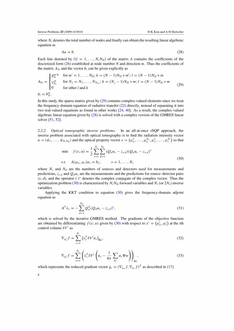
Figure 1. The schematic of the test problems 1 and 2: cylinder height H = 2 cm and radius r =1 cm. (a) Source–detector configuration: 8 sources ( ) and 64 detectors (◦), and (b) computationdomain with 6764 tetrahedrons.

3. Results

3.1. Numerical experiments

In this section, we show numerical results for reconstructions of the spatial distributions ofoptical properties inside the medium by using the rSQP method and the lm-BFGS method.Note that the lm-BFGS approach implemented in this study generates the quasi-Newtonmatrices using information from the last six iterations in a very efficient way by employing therecursive formula given in [32]. To illustrate the code performance, we compare the results ofboth schemes on three types of test problems, all with cylindrical geometries.

3.1.1. Setup of the test problems. The geometry for the first two cases in this study consistsof a cylinder with diameter of 2 cm and a height of 2 cm in which a smaller cylinder with adiameter of 0.5 cm is embedded (figure 1). This geometry mimics small animal experiments[12–15] or measurements on finger joints [9–11]. In the first example, the smaller cylinderdiffers in μa from the larger cylinder, while μs is the same (see table 1). The absorptioncoefficient of the smaller cylinder is set to be twice as high (μa = 0.2 cm−1) as that of thebackground medium (μa = 0.1 cm−1). Note that all sources and detectors are located ona circle defined by � = {(x, y, z)|x2 + y2 = 1, z = 1}. The second problem involves thereconstruction of μs . Therefore instead of varying μa inside the smaller cylinder, we nowincrease μs inside the smaller cylinder to 15 cm−1, while the background medium stays atμs = 10 cm−1.

In the third example, we consider the case of reconstructing μa and μs simultaneously.In this case, two spherical objects are embedded in a background medium that varies inboth the absorption coefficient μa and the scattering coefficient μs . The sources anddetectors are located on two circles, defined by � = {(x, y, z)|x2 + y2 = 1.52, z = 2.2}10

Inverse Problems 25 (2009) 015010 H K Kim and A H Hielscher

(a) (b)

r

H

Figure 2. The schematic of the test problem 3: cylinder height H = 5 cm, radius r = 1.5 cmand two embedded spherical objects with diameter of 0.5 cm. (a) Source–detector configurationat planes z = 2.2 cm and z = 3.2 cm: 24 sources ( ) and 24 detectors (◦), and (b) computationdomain with 14 114 tetrahedrons.

Table 1. Parameters used in three different examples.

Problem 1 Problem 2 Problem 3

Anisotropic factor g 0.0 0.5 0.9Background μa (cm−1) 0.1 0.1 0.5Inhomogeneity μa (cm−1) 0.2 0.1 1.0Background μs (cm−1) 10.0 10.0 10.0Inhomogeneity μs (cm−1) 10.0 15.0 15.0Number of sources 8 8 24Number of detectors 64 64 24Modulation frequency ω (MHz) 400 400 600Number of finite volumes 6764 6764 14 114Number of discrete ordinates 24 48 80

and � = {(x, y, z)|x2 + y2 = 1.52, z = 3.2}, respectively (see figure 2). The correspondingvalues of optical properties for all three cases are given in table 1.

For the numerical experiments, we use synthetic data that are obtained from the solutionof the frequency-domain forward problem given by (22) at specified detector locations forthe exact optical properties. All synthetic data are generated on a mesh that is two timesfiner than the mesh used for the reconstructions. The solution of the forward problem atdetector locations provides the exact ‘measurements’ zex. Measurements containing noise aresimulated by adding an error term to zex in the form zobs = zex + �σ , where σ is the standarddeviation of measurement errors and � is the random variable with normal distribution, zeromean and unitary standard deviation. With the use of such simulated measurements as theinput data for the inverse analysis, we examine the stability of the inverse solution with respectto various noise levels by generating data with different standard deviations obtained from thesignal-to-noise ratio, SNR = 10 log(z/σ ).

11

Inverse Problems 25 (2009) 015010 H K Kim and A H Hielscher

We stop the optimization process when the following stopping criteria are satisfied:

|f k+1(u; x) − f k(u; x)|/f k(u; x) � ε1, (34a)

f k(u; x) � ε2. (34b)

The tolerance ε1 is set to 10−5, and ε2 is chosen to have the same order of magnitude ofmeasurement errors, which leads to sufficiently stable results in the principle of discrepancy[53]. When noise-free data is considered, the tolerance ε2 is assigned a sufficiently smallnumber (typically 10−6). The stopping criteria given by (34a), (34b) are applied in the sameway to the reconstruction codes that make use of the rSQP method and the lm-BFGS method.

To quantify the quality of reconstruction, we use the correlation factor ρ(μe, μr) and thedeviation factor δ(μe, μr) as introduced in [21]:

ρ(μe, μr) =∑Nt

i=1

(μe

i − μei

)(μr

i − μri

)(Nt − 1)σ (μe)σ (μr)

, δ(μe, μr) =√∑Nt

i=1

(μe

i − μri

)2Nt

σ(μe). (35)

Here μ and σ(μ) are the mean value and the standard deviation for the spatial functionof the optical property than can be either μa and μs . Similarly, μe and μr are theexact and reconstructed distributions of optical properties, respectively. The correlationcoefficient indicates the degree of correlation between exact and estimated quantities while thedeviation factor describes the discrepancy in absolute values of exact and estimated quantities.Accordingly, the closer ρ(μe, μr) gets to unity, and the closer δ(μe, μr) gets to zero, the betteris the quality of the reconstruction.

In the following sections, the rSQP method and the lm-BFGS method are applied tofunctional estimations of unknown optical properties for the three test problems as given intable 1. All the simulations are carried out on a Pentium IV 3.0 GHz CPU processor.

3.1.2. CPU time and influence of noise. To compare the CPU time and the influence ofnoise in rSQP-based and lm-BFGS-based algorithms, we consider the reconstruction of μa

inside the target medium as shown in figure 1. We test the effects of noise on the algorithmby varying the SNR from infinity (no noise) to 20 dB and 15 dB, with the later two valuesrepresenting typical noise levels encountered in optical tomography [21].

As shown in table 2, the usage of the rSQP method results in a significant reduction ofcomputation time in all cases considered here. For the case of the noise-free data, the rSQPmethod converges in 0.44 h while the lm-BFGS method takes about 5 h to reach the sameconvergence criterion. Therefore, the rSQP method reduces the computation time by a factorof about 11. We observe a similar reduction in the two other cases of different noise levels.The 20 dB data requires 0.2 h using the rSQP method and 2.18 h using the lm-BFGS method,respectively. With the 15 dB data the rSQP method converges in 0.15 h while the lm-BFGSmethod requires 3.72 h. Therefore, in this case, using the rSQP method reduces computationtime by a factor of about 25.

The main reason for this significant reduction in CPU time can be explained by thefact that the rSQP method does not require the exact solution of the forward problem ateach iteration of optimization until it converges to the optimal solution, as mentioned earlier.Indeed we obtain the incomplete solution of the linearized forward equation by applying theloose tolerance of 10−2 that is empirically chosen from our extensive study. We found thateven a tolerance of 10−2 can generate a sequence of feasible solutions satisfying the first-order necessary conditions (KKT conditions), while advancing to the true solution throughthe optimization process. For example, we usually stop the GMRES iteration for the forward

12

Inverse Problems 25 (2009) 015010 H K Kim and A H Hielscher

(a) (b)

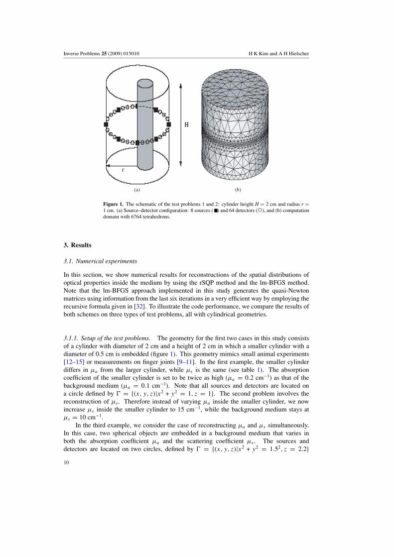
Figure 3. Variations of the value of the objective function (in log10 scale) obtained with the rSQPand lm-BFGS methods for the reconstruction μa with noise-free data. A convergence history foreach of the two methods is depicted with respect to (a) the number of function evaluations and(b) the CPU time.

Table 2. Comparison of the CPU time and the reconstruction quality for codes that make use ofrSQP and lm-BFGS methods. CPU time, rho and delta are given for varying noise levels in theinput data of problem 1 (see table 1).

Schemes CPU time (∗) Correlation ρ(μe, μr ) Deviation δ(μe, μr )

Noise free rSQP 0.44 h (11.5) 0.79 0.65

lm-BFGS 5.05 h 0.78 0.6520 dB rSQP 0.20 h (10.9) 0.63 0.93

lm-BFGS 2.18 h 0.64 0.8515 dB rSQP 0.15 h (24.8) 0.47 1.03

lm-BFGS 3.72 h 0.42 0.99

∗ denotes the acceleration factor by the rSQP method.

solution when its relative residual becomes smaller than 10−10. Thus the GMRES iterationprocess essentially has to perform a sufficient number of matrix-vector multiplications to reachthe desired accuracy, which is the case using the unconstrained lm-BFGS method. However,the rSQP scheme stops the GMRES iteration at a much earlier stage of the iterations basedon the loose tolerance. As a consequence, the rSQP scheme only requires a relatively smallernumber of matrix-vector multiplications, which leads to a significant time savings throughthe overall optimization process. Figures 3(a) and (b) show the convergence history of thetwo methods versus the number of function evaluations and the CPU times. As expected,it is observed that the rSQP scheme produces a similar convergence history with respect tothe iteration number (figure 3(a)) but it shows much faster convergence with respect to thecomputation time (figure 3(b)).

In addition to the CPU time, we measured the accuracy of reconstruction as a functionof the SNR. The correlation factor ρ(μe, μr) and the deviation factor δ(μe, μr) as defined in(35) are computed for the plane z = 1 where the sources and the detectors are located. Thecorresponding values of ρ(μe, μr) and δ(μe, μr) are given in table 2. Figure 4 shows thecross-section maps of the reconstructed μa for the xy-plane (first row in figure 4) at z = 1and the xz-plane (second row in figure 4) at y = 0. The upper and lower parts of the xz-planeimages contain the optical properties of the unchanged initial guess due to the lack of sources

13

Inverse Problems 25 (2009) 015010 H K Kim and A H Hielscher

(a) (c) (e)

(b) (d) (f)

Figure 4. Cross-section maps of the reconstructed μa-value obtained for problem 1 (see table 1).The maps are shown for the xy-plane at z = 1 and xz-plane at y = 0. (a) and (b) lm-BFGS resultswith noise-free data; (c) and (d) rSQP result with noise-free data; (e) and (f) rSQP reconstructionswith 15 dB noise-added data.

and detectors at these regions. As a result, one can observe the reconstructed object onlyaround the region where all sources and detectors are placed.

At noise levels of 15–20 dB, the difference between the rSQP and lm-BFGS methods arenot significant; both schemes show a decrease in the correlation factor and an increase in thedeviation factor as compared to the corresponding values of the noise-free data (∞ dB, seetable 2). Therefore, it can be stated that the rSQP and lm-BFGS methods are similar to eachother in terms of response to noise in the data.

3.1.3. Effect of initial guess. Typically the exact optical properties of the backgroundmedium are not known a priori, and the optimization scheme starts with certain reasonablechoice for these properties. It can be assumed that there is always some mismatch betweenthe true background medium and the guessed background medium, which can affect thereconstruction accuracy. For this reason, we evaluate the robustness of the rSQP code to thisinitial guess of optical properties.

For this study we consider the same geometry as the first example but this time we changeμs inside the smaller cylinder as shown in figure 1. The corresponding optical propertiesare given in table 1. We looked at two cases. First we assumed that the initial guess of thebackground optical properties is 10% higher than the true value; in the second example theinitial guess is 20% higher. The simulations are performed with noise-free data and CPU timesare measured. In addition, we calculated the correlation factor ρ(μe, μr) and the deviationfactor δ(μe, μr) to discuss the robustness of the rSQP and lm-BFGS codes to initial guess.The results are given in figure 5 and table 3.

It can be seen from table 3 that the rSQP method leads to much more accurate resultsthan the lm-BFGS method when the initial guesses of the optical properties of the background

14

Inverse Problems 25 (2009) 015010 H K Kim and A H Hielscher

(a) (c) (e)

(b) (d) (f)

Figure 5. Cross-section maps of the reconstructed μs value for problem 2 (see table 1) obtainedby using the rSQP method. Maps shown represent result for the xy-plane at z = 1.0 andxz-plane at y = 0, respectively. (a) and (b) Reconstruction results based on noise-free data;(c) and (d) reconstruction results obtained by starting with initial guess of optical properties that is10% higher than true optical properties; (e) and (f) reconstruction results obtained by starting withinitial guess of optical properties that is 20% higher than true optical properties.

Table 3. The reconstruction quality and the computation time obtained with the two methods fordifferent initial guesses for the second example of reconstructing μs .

Schemes CPU time (∗) Correlation ρ(μe, μr ) Deviation δ(μe, μr )

Background RSQP 4.3 h (12.2) 0.89 0.57

lm-BFGS 52.4 h 0.88 0.5310% higher RSQP 3.7 h (16) 0.78 0.73

lm-BFGS 59.2 h 0.62 0.8720% higher RSQP 3.6 h (16.9) 0.53 0.98

lm-BFGS 60.8 h 0.41 1.69

∗ denotes the acceleration factor by the rSQP method.

medium are 10% or 20% higher. The correlation factor ρ(μe, μr) using the rSQP methodis 0.78 and 0.53 for the 10% and 20% cases, respectively. This is almost 20% better thanwhen the lm-BFGS method is used (ρ(μe, μr) = 0.62 and 0.41, respectively). Also the rSQPmethod shows 20–50% smaller deviation factors (δ(μe, μr) = 0.73 and 0.98 for 10% and20% cases, respectively), as compared to the lm-BFGS method (δ(μe, μr) = 0.87 and 1.69).

Furthermore, the CPU times are 16 times shorter (3.7 h as compared to 59.2 h in 10% case,and 3.6 h versus 60.8 h in 20% case). We also observed that the rSQP method still converges toreasonable solutions even when initial guess is made 50% larger than the true value, whereasthe lm-BFGS method leads to a premature convergence for this same case. The reason forthis observation is not quite clear but may be understood by looking at how the variables aretreated in these two different schemes. The unconstrained scheme treats the intensity vector uas a dependent variable of the model parameter vector x, while the PDE-constrained scheme

15

Inverse Problems 25 (2009) 015010 H K Kim and A H Hielscher

(a)

(b) (c)

(d)

(e) (f)

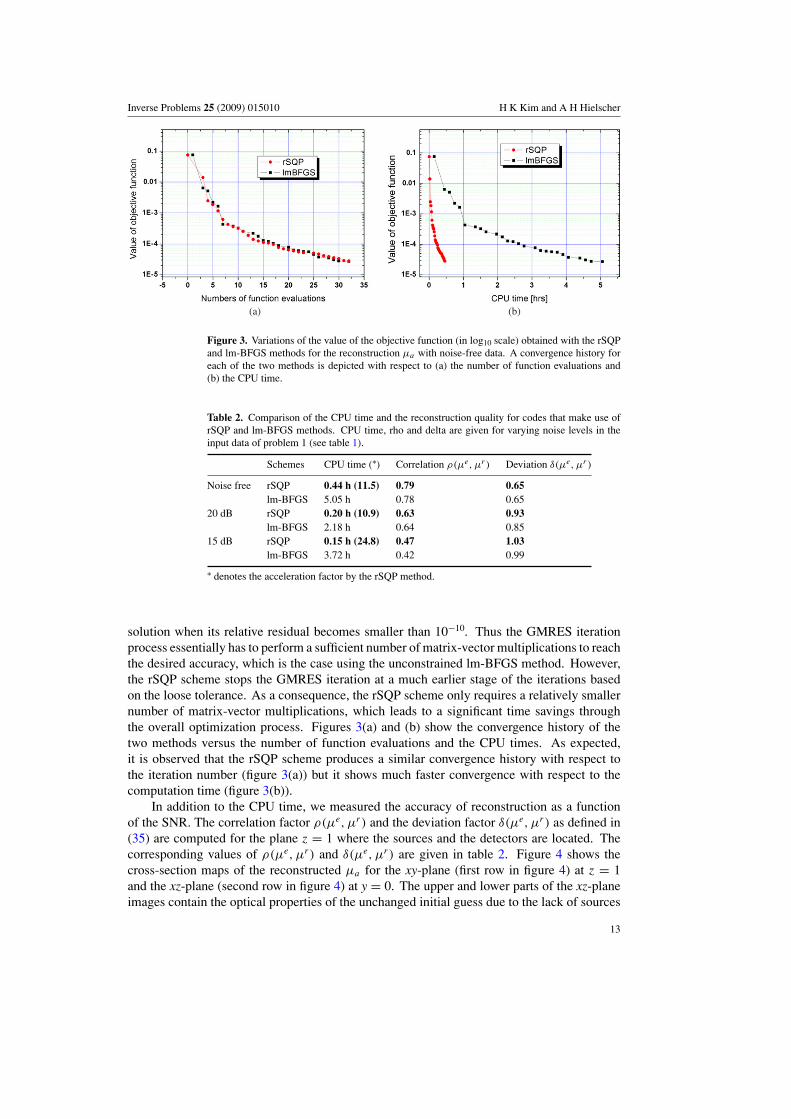
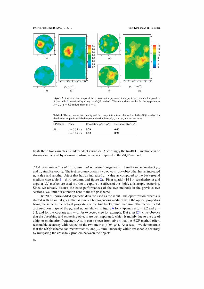
Figure 6. Cross-section maps of the reconstructed μa(a) –(c) and μs (d)–(f) values for problem3 (see table 1) obtained by using the rSQP method. The maps show results for the xy-planes atz = 2.2, z = 3.2 and xz-plane at y = 0.

Table 4. The reconstruction quality and the computation time obtained with the rSQP method forthe third example in which the spatial distributions of μa and μs are reconstructed.

CPU time Plane Correlation ρ(μe, μr ) Deviation δ(μe, μr )

51 h z = 2.25 cm 0.79 0.60

z = 3.25 cm 0.53 0.92

treats these two variables as independent variables. Accordingly the lm-BFGS method can bestronger influenced by a wrong starting value as compared to the rSQP method.

3.1.4. Reconstruction of absorption and scattering coefficients. Finally we reconstruct μa

and μs simultaneously. The test medium contains two objects: one object that has an increasedμa value and another object that has an increased μs value as compared to the backgroundmedium (see table 1—third column, and figure 2). Finer spatial (14 114 tetrahedrons) andangular (S8) meshes are used in order to capture the effects of the highly anisotropic scattering.Since we already discuss the code performances of the two methods in the previous twosections, we limit our attention here to the rSQP scheme.

The 20 dB noise-added synthetic data are used as the input. The optimization process isstarted with an initial guess that assumes a homogeneous medium with the optical propertiesbeing the same as the optical properties of the true background medium. The reconstructedcross-section maps of the μa and μs are shown in figure 6 for xy-planes at z = 2.2 and z =3.2, and for the xz-plane at y = 0. As expected (see for example, Kui et al [24]), we observethat the absorbing and scattering objects are well separated, which is mainly due to the use ofa higher modulation frequency. Also it can be seen from table 4 that the rSQP method offersreasonable accuracy with respect to the two metrics ρ(μe, μr). As a result, we demonstratethat the rSQP scheme can reconstruct μa and μs simultaneously within reasonable accuracyby mitigating the cross-talk problem between the objects.

16

Inverse Problems 25 (2009) 015010 H K Kim and A H Hielscher

(a) (b)

Figure 7. Schematic of the phantom used for experimental studies; (a) locations of 25 sources(•) and 25 detectors (•), (b) the computation domain with 28 852 tetrahedrons. The diameter of acylinder is 3.2 cm and the height 3.6 cm.

1.45

0.06

(a)

μa[cm-1]

(b)

μa[cm-1]

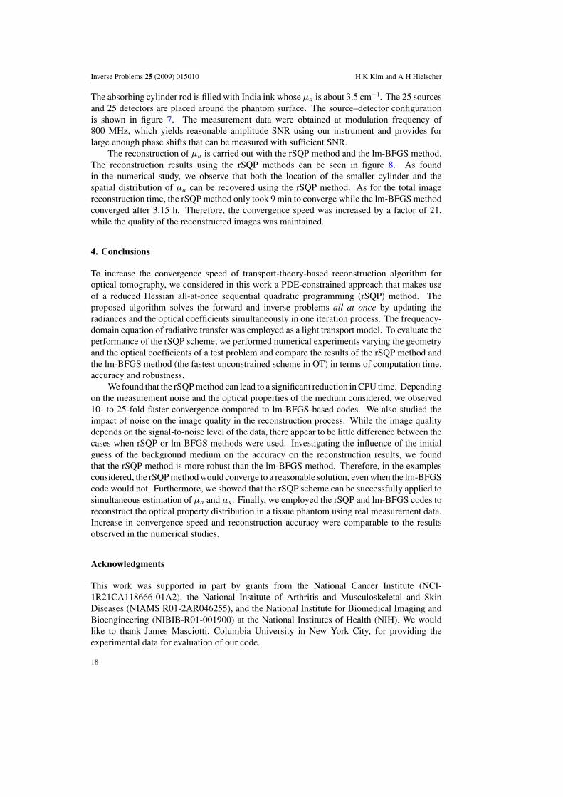
Figure 8. Cross-section maps of the reconstructed-μa value using experimental data obtained at800 MHz with the tissue phantom shown in figure 7. Reconstruction results were generated withthe rSQP code and results are shown for the xy-plane at z = 1.8 (a) and the yz-plane at x = 0 (b).

3.2. Application to experimental data

In addition to the numerical studies, we also apply our code to experimental data. For theexperimental studies we use a tissue phantom with optical properties similar to those usedin the numerical studies. A cylinder with a 3.2 cm diameter (figure 7) is filled with 0.55%intralipid. The anisotropy of intralipid g is 0.71. The reduced scattering coefficient ofintralipid is μ′

s = 3.5 cm−1. The absorption coefficient of the background is known as μa =0.027 cm−1. The perturbation consists of a simple absorption inclusion rod (with the samescattering properties as the background) placed vertically about 1 cm away from the surface.

17

Inverse Problems 25 (2009) 015010 H K Kim and A H Hielscher

The absorbing cylinder rod is filled with India ink whose μa is about 3.5 cm−1. The 25 sourcesand 25 detectors are placed around the phantom surface. The source–detector configurationis shown in figure 7. The measurement data were obtained at modulation frequency of800 MHz, which yields reasonable amplitude SNR using our instrument and provides forlarge enough phase shifts that can be measured with sufficient SNR.

The reconstruction of μa is carried out with the rSQP method and the lm-BFGS method.The reconstruction results using the rSQP methods can be seen in figure 8. As foundin the numerical study, we observe that both the location of the smaller cylinder and thespatial distribution of μa can be recovered using the rSQP method. As for the total imagereconstruction time, the rSQP method only took 9 min to converge while the lm-BFGS methodconverged after 3.15 h. Therefore, the convergence speed was increased by a factor of 21,while the quality of the reconstructed images was maintained.

4. Conclusions

To increase the convergence speed of transport-theory-based reconstruction algorithm foroptical tomography, we considered in this work a PDE-constrained approach that makes useof a reduced Hessian all-at-once sequential quadratic programming (rSQP) method. Theproposed algorithm solves the forward and inverse problems all at once by updating theradiances and the optical coefficients simultaneously in one iteration process. The frequency-domain equation of radiative transfer was employed as a light transport model. To evaluate theperformance of the rSQP scheme, we performed numerical experiments varying the geometryand the optical coefficients of a test problem and compare the results of the rSQP method andthe lm-BFGS method (the fastest unconstrained scheme in OT) in terms of computation time,accuracy and robustness.

We found that the rSQP method can lead to a significant reduction in CPU time. Dependingon the measurement noise and the optical properties of the medium considered, we observed10- to 25-fold faster convergence compared to lm-BFGS-based codes. We also studied theimpact of noise on the image quality in the reconstruction process. While the image qualitydepends on the signal-to-noise level of the data, there appear to be little difference between thecases when rSQP or lm-BFGS methods were used. Investigating the influence of the initialguess of the background medium on the accuracy on the reconstruction results, we foundthat the rSQP method is more robust than the lm-BFGS method. Therefore, in the examplesconsidered, the rSQP method would converge to a reasonable solution, even when the lm-BFGScode would not. Furthermore, we showed that the rSQP scheme can be successfully applied tosimultaneous estimation of μa and μs . Finally, we employed the rSQP and lm-BFGS codes toreconstruct the optical property distribution in a tissue phantom using real measurement data.Increase in convergence speed and reconstruction accuracy were comparable to the resultsobserved in the numerical studies.

Acknowledgments

This work was supported in part by grants from the National Cancer Institute (NCI-1R21CA118666-01A2), the National Institute of Arthritis and Musculoskeletal and SkinDiseases (NIAMS R01-2AR046255), and the National Institute for Biomedical Imaging andBioengineering (NIBIB-R01-001900) at the National Institutes of Health (NIH). We wouldlike to thank James Masciotti, Columbia University in New York City, for providing theexperimental data for evaluation of our code.

18

Inverse Problems 25 (2009) 015010 H K Kim and A H Hielscher

References

[1] Xu Y, Graber H L and Barbour R L 2007 Image correction algorithm for functional three-dimensional diffuseoptical tomography brain imaging Appl. Opt. 46 1693–704

[2] Joseph D K, Huppert T J, Franceschini M A and Boas D A 2006 Diffuse optical tomography system to imagebrain activation with improved spatial resolution and validation with functional magnetic resonance imagingAppl. Opt. 45 8142–51

[3] Boas D A, Chen K, Grebert D and Franceschini M A 2004 Improving the diffuse optical imaging spatialresolution of the cerebral hemodynamic response to brain activation in humans Opt. Lett. 29 1506

[4] Hebden J C, Gibson A P, Austin T, Yusof R M, Everdell N, Delpy D T, Arridge S R, Meek J H and Wyatt J S2004 Imaging changes in blood volume and oxygenation in the newborn infant brain using three-dimensionaloptical tomography Phys. Med. Biol. 49 1117–30

[5] Blueston A, Abdoulaev G S, Schmitz C, Barbour R and Hielscher A H 2001 Three-dimensional opticaltomography of hemodynamics in the human head Opt. Express 9 272

[6] Davis S C, Dehghani H, Wang J, Jiang S, Pogue B W and Paulsen K D 2007 Image-guided diffuse opticalfluorescence tomography implemented with Laplacian-type regularization Opt. Express 15 4066–82

[7] Corlu A, Choe R, Durduran T, Rosen M A, Schweiger M, Arridge S A, Schnall M D and Yodh A G 2007 Three-dimensional in vivo fluorescence diffuse optical tomography of breast cancer in humans Opt. Express 15 6696

[8] Choe R et al 2005 Diffuse optical tomography of breast cancer during neoadjuvant chemotherapy: a case studywith comparison to MRI Med. Phys. 32 1128–39

[9] Hielscher A H, Klose A D, Scheel A, Moa-Anderson B, Backhaus M, Netz U and Beuthan J 2004 Sagittal laseroptical tomography for imaging of rheumatoid finger joints Phys. Med. Biol. 49 1147

[10] Scheel A K, Backhaus M, Klose A D, Moa-Anderson B, Netz U J, Hermann K G, Beuthan J, Muller G A,Burmester G R and Hielscher A H 2004 First clinical evaluation of sagittal laser optical tomography fordetection of synovitis in arthritic finger joints Ann. Rheum. Dis. 64 239–45

[11] Zhang Q and Jiang H 2005 Three-dimensional diffuse optical tomography of simulated hand joints with a 64 ×64-channel photodiodes-based optical system J. Opt. A Pure Appl. Opt. 7 224–31

[12] Hielscher A H 2005 Optical tomographic imaging of small animals Curr. Opin. Biotechnol. 16 79–88[13] Xu H, Springett R, Dehghani H, Pogue B W, Paulsen K D and Dunn J F 2005 Magnetic-resonance-imaging-

coupled broadband near-infrared tomography system for small animal brain studies Appl. Opt. 44 2177–88[14] Bluestone A Y, Stewart M, Lei B, Kass I S, Lasker J, Abdoulaev G S and Hielscher A H 2004 Three-dimensional

optical tomographic brain imaging in small animals: Part I. Hypercapnia J. Biomed. Opt. 9 1046–62[15] Bluestone A Y, Stewart M, Lasker J, Abdoulaev G S and Hielscher A H 2004 Three-dimensional optical

tomographic brain imaging in small animals: Part II. Unilateral carotid occlusion J. Biomed. Opt. 9 1063–73[16] Arridge S R 1999 Optical tomography in medical imaging Inverse Problems 15 R41–93[17] Hielscher A H, Klose A D and Hanson K M 1999 Gradient-based iterative image reconstruction scheme for

time-resolved optical tomography IEEE Trans. Med. Imaging 18 262–71[18] Yao Y Q, Wang Y, Pei Y L, Zhu W W and Barbour R L 1997 Frequency-domain optical imaging of absorption

and scattering distributions by Born iterative method J. Opt. Soc. Am. A 14 325–42[19] Ye J C, Webb K J, Bouman C A and Millane R P 1999 Optical diffusion tomography by iterative-coordinate-

descent optimization in a Bayesian framework J. Opt. Soc. Am. A 16 2400–12[20] Ripoll J and Ntziachristos V 2003 Iterative boundary method for diffuse optical tomography J. Opt. Soc. Am.

A 20 1103–10[21] Klose A D and Hielscher A H 2003 Quasi-newton methods in optical tomographic image reconstruction Inverse

Problems 19 309–87[22] Roy R and Sevick-Muraca E M 2000 Active constrained truncated Newton method for simple-bound optical

tomography J. Opt. Soc. Am. A 17 1627–41[23] Intes X, Ntziachristos V, Culver J P, Yodh A and Chance B 2002 Projection access order in algebraic

reconstruction technique for diffuse optical tomography Phys. Med. Biol. 47 N1–10[24] Ren R, Bal G and Hielscher A H 2006 Frequency domain optical tomography with the equation of radiative

transfer SIAM J. Sci. Comput. 28 1463–89[25] Kim H K and Charette A 2007 A sensitivity function-based conjugate gradient method for optical

tomography with the frequency-domain equation of radiative transfer J. Quantum Spectrosc. RadIat. Transfer104 24–39

[26] Schweiger M, Arridge S and Nassila I 2005 Gauss–Newton method for image reconstruction in diffuse opticaltomography Phys. Med. Biol. 50 2365–86

[27] Hielscher A H, Alcouffe A E and Barbour R L 1998 Comparison of finite-difference transport and diffusioncalculations for photon migration in homogeneous and heterogeneous tissues Phys. Med. Biol. 43 1285–302

19

Inverse Problems 25 (2009) 015010 H K Kim and A H Hielscher

[28] Roy R, Godavarty A and Sevick-Muraca E M 2003 Fluorescence-enhanced optical tomography using referencedmeasurements of heterogeneous media IEEE Trans. Med. Imaing 22 824–36

[29] Roy R and Sevick-Muraca E M 2001 Three-dimensional unconstrained and constrained image-reconstructiontechniques applied to fluorescence, frequency-domain photon migration Appl. Opt. 40 2206

[30] Hielscher A and Bartel S 2001 Use of penalty terms in gradient-based iterative reconstruction schemes foroptical tomography J. Biomed. Opt. 6 183

[31] Yalavarthy P K, Pogue B W, Dehghani H, Carpenter C M, Jiang S and Paulsen K D 2007 Structural informationwithin regularization matrices improves near infrared diffuse optical tomography Opt. Express 15 8043–58

[32] Nocedal J and Wright S J 2006 Numerical Optimization (New York: Springer)[33] Heinkenschloss M 1996 Projected sequential quadratic programming methods SIAM J. Optim. 6 373–417[34] Byrd R, Curtis F and Nocedal J 2008 An inexact SQP method for equality constrained optimization SIAM J.

Optim. 19 351–69[35] Gill P, Murray W and Saunders M 2005 SNOPT: an SQP algorithm for large-scale constrained optimization

SIAM Rev. 47 99–131[36] Biros G and Ghattas O 2003 Parallel Lagrange–Newton–Krylov–Schur methods for PDE-constrained

optimization: Part I. The Krylov–Schur solver SIAM J. Sci. Comput. 27 687–713[37] Biegler L, Schmid C and Ternet D 1997 A Multiplier-Free, Reduced Hessian Method For Process Optimization,

Large-Scale Optimization with Applications: Part II. Optimal Design and Control (New York: Springer)p 101

[38] Haber E and Ascher U 2001 Preconditioned all-at-once methods for large, sparse parameter estimation problemsInverse Problems 17 1847

[39] Bonnas J, Gilbert J, Lemarechal C and Sagastizabal C 2003 Numerical optimization: theoretical and practicalaspects (New York: Springer)

[40] Abddoulaev G S, Ren K and Hielscher A H 2005 Optical tomography as a PDE-constrained optimizationproblem Inverse Problems 21 1507–30

[41] Burger M and Muhlhuber W 2002 Iterative regularization of parameter identification problems by sequentialquadratic programming methods Inverse Problems 18 943–69

Boggs P and Tolle J 2000 Sequential quadratic programming for large-scale nonlinear optimization J. Comput.Appl. Math. 124 123–37

[42] Hu JL, Wu Z, McCann H, Davis L E and Xie CG 2005 Sequential quadratic programming method for solutionof electromagnetic inverse problems IEEE Trans. Antennas Propag. 53 2680

[43] Feng D and Pulliam T 1995 All at-at-once reduced Hessian SQP scheme for aerodynamics design optimizationTechnical Report NASA Ames Research Center

[44] Coleman T, Liu J and Yuan W 2000 A quasi-newton quadratic penalty method for minimization subject tononlinear equality constraints Comput. Optim. Appl. 15 103–23

[45] Lalee M, Nocedal J and Plantenga T 2003 On the implementation of an algorithm for large-scale equalityconstrained optimization SIAM J. Optim. 8 682–706

[46] Biegler L, Nocedal J, Schmid C and Ternet D 2000 Numerical experience with a reduced Hessian method forlarge scale constrained optimization Comput. Optim. Appl. 15 45–67

[47] Henyey L G and Greenstein L J 1941 Diffuse radiation in the galaxy Astrophysics 90 70[48] Modest M 2003 Radiative Heat Transfer (New York: McGraw-Hill)[49] Minkowycz S, Sparrow E and Murthy J 2006 Handbook of Numerical Heat Transfer (Hoboken, NJ: Wiley)[50] Meese E A 1998 Finite volume methods for the incompressible Navier–Stokes equations on unstructured grids

Ph.D. Thesis Norwegian University of Science and Technology, Trondheim, Norway[51] Saad Y 2003 Iterative Methods for Sparse Linear Systems (Philadelphia: SIAM)[52] Saad Y and Schultz M H 1986 GMRES: a generalized minimal residual algorithm for solving nonsymmetric

linear systems SIAM J. Sci. Stat. Comput. 3 856–69[53] Alifanov O M 1994 Inverse Heat Transfer Problems (New York: Springer)

20