WP/07/202

A Party without a Hangover? On the Effects of U.S. Government Deficits

Michael Kumhof and Douglas Laxton

© 2007 International Monetary Fund WP/07/202 IMF Working Paper Research Department

A Party without a Hangover? On the Effects of U.S. Government Deficits

Prepared by Michael Kumhof and Douglas Laxton

Authorized for distribution by Gian Maria Milesi-Ferretti

August 2007

Abstract

This Working Paper should not be reported as representing the views of the IMF. The views expressed in this Working Paper are those of the author(s) and do not necessarily represent those of the IMF or IMF policy. Working Papers describe research in progress by the author(s) and are published to elicit comments and to further debate.

This paper develops a 2-country New Keynesian overlapping generations model suitable for the joint evaluation of monetary and fiscal policies. We show that a permanent increase in U.S. government deficits raises the world real interest rate and significantly increases U.S. current account deficits, especially in the medium- to long-run. A simultaneous increase in non-U.S. savings lowers the world real interest rate and further increases U.S. current account deficits. We show that conventional infinite horizon models are ill-equipped to deal with issues that involve permanent changes in public or private sector savings rates. JEL Classification Numbers: E62; F41; F42; H30; H63 Keywords: Finite Lives; Distortionary Taxes; Government Debt Authors’ E-Mail Addresses: mkumhof@imf.org; dlaxton@imf.org

- 2 -

Contents

I. Introduction . . . . . . . . . . . . . . . . . . . . . . . . . . . . . . . . . . . . . 3

II. The Model . . . . . . . . . . . . . . . . . . . . . . . . . . . . . . . . . . . . . . 6A. Households . . . . . . . . . . . . . . . . . . . . . . . . . . . . . . . . . . . 8

1. Overlapping Generations Households . . . . . . . . . . . . . . . . . 82. Liquidity Constrained Households . . . . . . . . . . . . . . . . . . . 123. Aggregate Household Sector . . . . . . . . . . . . . . . . . . . . . . 12

B. Firms and Unions . . . . . . . . . . . . . . . . . . . . . . . . . . . . . . . 121. Manufacturers . . . . . . . . . . . . . . . . . . . . . . . . . . . . . . 132. Unions . . . . . . . . . . . . . . . . . . . . . . . . . . . . . . . . . . 143. Import Agents . . . . . . . . . . . . . . . . . . . . . . . . . . . . . . 144. Distributors . . . . . . . . . . . . . . . . . . . . . . . . . . . . . . . 155. Retailers . . . . . . . . . . . . . . . . . . . . . . . . . . . . . . . . . 16

C. Government . . . . . . . . . . . . . . . . . . . . . . . . . . . . . . . . . . 161. Fiscal Policy . . . . . . . . . . . . . . . . . . . . . . . . . . . . . . . 162. Monetary Policy . . . . . . . . . . . . . . . . . . . . . . . . . . . . . 17

D. Equilibrium and Balance of Payments . . . . . . . . . . . . . . . . . . . . 17

III. Calibration . . . . . . . . . . . . . . . . . . . . . . . . . . . . . . . . . . . . . . 18

IV. Implications of U.S. Government Deficits . . . . . . . . . . . . . . . . . . . . . 21A. Useful Steady-State Relationships . . . . . . . . . . . . . . . . . . . . . . 21B. The Quantitative Predictions of the Two Models . . . . . . . . . . . . . . 22

V. Implications of Government Spending Cuts . . . . . . . . . . . . . . . . . . . . 25

VI. Implications of Private Sector Savings Behavior . . . . . . . . . . . . . . . . . 26

VII. Conclusion . . . . . . . . . . . . . . . . . . . . . . . . . . . . . . . . . . . . . . 27 References . . . . . . . . . . . . . . . . . . . . . . . . . . . . . . . . . . . . . . . . . . 35

Figures

1. Savings, Investment and Current Account Balances: U.S. and the Rest of theWorld . . . . . . . . . . . . . . . . . . . . . . . . . . . . . . . . . . . . . . . . . 28

2. Real Interest Rates and EMBI Spreads . . . . . . . . . . . . . . . . . . . . . . 293. Sources of National Savings in the United States . . . . . . . . . . . . . . . . . 294. Flow Chart of the Model . . . . . . . . . . . . . . . . . . . . . . . . . . . . . . 305. Permanent Increase in Government Debt in OLG and REP - Part I . . . . . . 316. Permanent Increase in Government Debt in OLG and REP - Part II . . . . . . 327. Cuts in Government Investment and Consumption . . . . . . . . . . . . . . . . 338. Lower U.S. Rate of Time Preference and Higher RW Rate of Time Preference 34

- 3 -

I. Introduction

The short-term expansionary effects of fiscal deficits and the medium- and long-termcrowding-out effects of the resulting increased government debt continue to be topics ofconsiderable interest in both policymaking and academic circles. In an age of increasingmacroeconomic interdependence across countries this interest is no longer exclusivelymotivated by the study of individual economies, but also by spillovers between multipleeconomies.1 Probably the most pressing example, and the subject of this paper, is theconcern with U.S. fiscal deficits in the context of global current account imbalances. Thequestion we ask, and attempt to answer with the help of a new non-Ricardian model, iswhether the post-2001 deterioration in U.S. fiscal balances should be seen as a majorcontributing factor to the simultaneous further deterioration in U.S. current accountbalances. Or conversely, would a U.S. fiscal consolidation make a sizeable contribution tothe resolution of global current account imbalances?

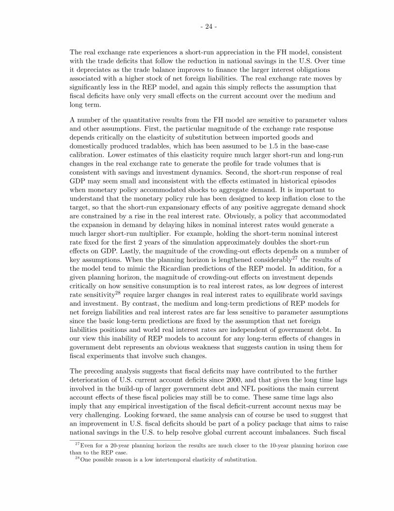
It is important to emphasize that U.S. fiscal policy has been only one of the driversaffecting the U.S. current account deficit, and that higher national savings rates in the restof the world have probably been even more important. Figure 1 summarizes recent trendsin savings and investment flows in the U.S. and the rest of the world. To understand theimpact of world savings on world real interest rates, Figure 2 plots the short-term realinterest rate for the U.S. and for a group of advanced economies excluding the U.S., aswell as a measure of spreads for emerging-market economies. The first importantobservation is that over the last few years national savings have increased significantly inthe rest of the world, accompanied by real interest rates that have trended down in allmajor regions of the world. This supports Bernanke’s (2005) hypothesis that the world isexperiencing a “savings glut”, and that this has been responsible for a large part of theincrease in the U.S. current account deficit. Due to many differences in individualcountries’ accounting conventions, it is difficult to consistently decompose national savingsin the rest of the world into public and private savings.2 However, detailed fiscal data areavailable for the U.S., and are shown in Figure 3. These data suggest that since 2001lower U.S. public savings have reduced national savings, which confirms that U.S. fiscalpolicy should be another candidate explanation for larger U.S. current account deficits.

Recent model-based estimates of the effects of U.S. fiscal deficits derived from the FederalReserve Board’s SIGMA model and the IMF’s Global Economy Model (GEM) haveattracted considerable attention in policymaking circles.3 The estimates from both ofthese institutions are based on a new generation of open economy monetary business cyclemodels with both nominal and real rigidities that are being deployed rapidly in centralbanks to replace the previous generation of models, which were not completely based on

1See, for example, Chinn (2005), Chinn and Ito (2005), Chinn and Lee (2005), Chinn and Steil (2006),Kopcke, Tootell and Triest (2004) and Truman (2006).

2 In a recent paper Ferrero (2006) studies the effects of fiscal deficits in the U.S. relative to fiscal deficitsoutside the U.S. However, his fiscal data are restricted to the G6 and do not account for the recent increasein public savings in emerging Asia and the oil-exporting economies.

3For documentation on SIGMA see Erceg, Guerrieri and Gust, (2005a, b) and for GEM see Faruqeeand others (2005). For applications to policymaking discussions see, for example, Bernanke (2005) andpublications of the IMF’s World Economic Outlook by Laxton and Milesi-Ferretti (2005) and Kumhof andLaxton (2006).

- 4 -

microfoundations.4 Such models are well suited to address many monetary business cycleissues, but as argued in several important papers they face difficulties in adequatelyreplicating the dynamic short-run effects of fiscal policy.5 More importantly for thispaper, they have serious shortcomings when applied to the analysis of medium- andlong-run fiscal issues such as the crowding-out effects of a permanent increase in publicdebt.6 Indeed, the prediction of both SIGMA and GEM is that U.S. fiscal deficits (andrest of the world fiscal surpluses) should have very small medium- and long-run effects onthe current account balance and on world savings. It is important to emphasize that theresults of the IMF analysis using GEM suggest larger and more sustained effects than theFederal Reserve Board’s SIGMA model because the IMF’s scenarios assume that thedesired net foreign liability position will shift in response to higher levels of governmentdebt–see Faruqee and others (2005).

In view of the importance of fiscal policy problems, the idea of bringing models withmicrofoundations as rigorous as those of open economy monetary business cycle models tothe analysis of fiscal policy is very appealing.7 But to do so in a way that does not ignorethe critical interactions between monetary and fiscal policies, the microfoundations ofnon-Ricardian household and firm behavior need to be built while maintaining thenominal and real rigidities of existing models.

The candidate non-Ricardian features known from the literature are overlappinggenerations models following Blanchard (1985) and Weil (1989) and infinite horizonmodels with a subset of liquidity constrained agents following Gali, López-Salido andVallés (2007). Both model classes are capable of producing powerful short-run effects offiscal policy. But only an overlapping generations structure produces medium- andlong-run crowding out effects of government debt, and thereby endogenously determinesnet foreign liability positions as a function of government debt. Both of these effects areclearly critical to understanding the connection between fiscal and current account deficitsthat is the object of our study. An overlapping generations structure is therefore a keyingredient of this paper.

Bringing an overlapping generations setting into an open economy monetary businesscycle model has been undertaken by Ghironi (2000a,b) and by Ganelli (2005). The formerdoes not consider the effects of government debt, but shows that an overlappinggenerations structure following Blanchard (1985) and Weil (1989) ensures the existence ofa well-defined steady state for net foreign liability positions (see also Buiter (1981)). Ourmodel bears the closest resemblance to Ganelli (2005), which is the first attempt toanalyze alternative fiscal policies in an open economy monetary business cycle model withfinite lives.8 Our model adds to this several additional non-Ricardian features, a verygeneral specification of preferences and technologies, and a number of nominal and realrigidities that are critical for the quantitative implications of our policy simulations. Weshow that the resulting model, which is built on complete optimizing foundations, neststhe extreme Ricardian predictions of models such as SIGMA and GEM when the planning

4The related literature is very large. For some examples see Obstfeld and Rogoff (1995, 1996), Betts andDevereux (2001), Caselli(2001), Corsetti and Pesenti (2001), Ganelli (2003) and Laxton and Pesenti (2003).

5See Fatas and Mihov (2001), Blanchard and Perotti (2002), Gali, López-Salido and Vallés (2007).6We think of the medium-run as encompassing the period between 5 and 25 years after a shock.7See Ganelli and Lane (2002) for a discussion of the need to give a greater role to fiscal policy.8Ganelli (2005) is in turn related to the work of Frenkel and Razin (1992).

- 5 -

horizon is assumed to be infinite. But with finite horizons any change in taxes and debthas very significant real effects.

Our model has four non-Ricardian features. First, it features overlapping generationsagents with finite economic lifetimes. This implies that today’s agents discount future taxliabilities at a higher rate than the market real interest rate, because they attach asignificant probability to not becoming responsible for them. Second, the model exhibits astylized form of lifecycle income patterns whereby the average agent exhibits declininglabor productivity throughout his lifetime. He therefore discounts future labor income taxliabilities at an even higher rate because he expects to be supplying less effective labor inthe future. Third, the model features liquidity constrained (but nonetheless optimizing)agents who do not have access to financial markets to smooth consumption, so that theyhave to vary their consumption one-for-one with their after-tax income. And fourth, laborand consumption taxes are distortionary because labor effort and consumption respond torelative price movements that result directly from tax wedges.

Because one possible option for future fiscal consolidation consists of spending cuts ratherthan tax increases, we are also interested in a meaningful analysis of the spendingcomponent of fiscal policy. In this context, another important simplifying assumption ofmodels such as SIGMA and GEM is that all government expenditures are wasted and donot add to productive capacity. This is clearly far too simple for a complete analysis ofthe potential costs that would be associated with future government spending cuts. Wetherefore also extend the standard model to allow for government investment inproductive infrastructure.

As for preferences and technologies, a CRRA utility function allows us to highlight thecritical role of the intertemporal elasticity of substitution in the propagation of fiscalshocks.9 Furthermore, the labor supply decision is endogenous. Another critical ingredientis endogenous capital formation, which provides an additional channel through whichgovernment debt crowds out economic activity. The specification of technology containsboth traded and nontraded goods. Furthermore, the model economy features a full set ofnominal and real rigidities typical of existing monetary business cycle models. Nominalrigidities go beyond the simple case of one-period price rigidities to allow for meaningfulbusiness cycle dynamics. They include multiple levels of sticky goods prices as well assticky nominal wages. Real rigidities include habit persistence in consumption, investmentadjustment costs, and import adjustment costs.

The combination of non-Ricardian features and rigidities allows us to introducespecifications of fiscal and monetary policy that interact with one another. A monetarypolicy reaction function familiar from state-of-the-art monetary theory stabilizes inflationand output, while fiscal policy stabilizes the government balance and therefore governmentdebt. The short-run dynamics of the model are determined by the interaction of both ofthese policies, while the medium- and long-run dynamics depend only on fiscal policy.

9Previous overlapping generations models have often used log preferences to avoid complications duringaggregation.

- 6 -

The remainder of the paper is organized as follows. Section 2 summarizes the theoreticalstructure of the model, leaving some of the details to a Technical Appendix. Section 3discusses a base-case calibration. Section 4 compares the model’s short-run and long-runpredictions for the consequences of higher government deficits and government debt withthe predictions of a standard infinite horizon model augmented with liquidity-constrainedconsumers. We show that the two models behave very similarly in the very short run. Butin the infinite horizon model the medium- and long-run effects of higher government debtare negligible, while in the finite horizon model, under plausible assumptions aboutagents’ planning horizons, there is an economically highly significant link between highergovernment deficits and larger current account deficits, accompanied also by crowding outeffects on physical capital stocks. Turning to scenarios of fiscal consolidation, Section 5compares the implications of permanent cuts in government investment and governmentconsumption, showing that the former permanently reduces output while the latter raisesit. Section 6 studies the role of private sector savings behavior. We conclude that anincrease in rest of the world savings is likely to be playing a key role, as it is consistentwith not only U.S. current account deficits but also with the observed low world realinterest rate. Section 7 concludes.

II. The Model

The world consists of 2 countries, the United States (U.S.) and the rest of the world(RW). The flow of goods and factors between the different domestic sectors, and betweenthe two economies, is illustrated in Figure 4. When discussing the behavior of agents inone country alone we will not identify the country by additional notation. When theinteraction between two countries is discussed we identify the U.S. by an asterisk.

Each country is populated by two types of households, both of which consume finalretailed output and supply labor to unions. First, there are overlapping generationshouseholds (OLG) with finite planning horizons as in Blanchard (1985), and exhibitingexternal habit persistence. In each period, n∗(1− ψ∗)(1− θ) and n(1− ψ)(1− θ) of suchindividuals are born in the U.S. and RW, respectively. Second, there are liquidityconstrained households (LIQ) who do not have access to financial markets, and whoconsequently are forced to consume their after tax income in every period. The number ofsuch agents born in each period in the U.S. and in RW is n∗ψ∗(1− θ) and nψ(1− θ). Eachagent faces a constant probability of death (1− θ) in each period, which implies anaverage planning horizon of 1/ (1− θ).10 This implies that the total number of agents inthe U.S. and in RW is n∗ and n. In addition to the probability of death households alsoexperience labor productivity that declines at a constant rate over their lifetimes.11

Lifecycle income adds another powerful channel through which fiscal policies havenon-Ricardian effects. Households of both types are subject to a uniform labor income taxand a uniform consumption tax.

10 In general we allow for the possibility that agents may be more myopic than what would be suggestedby a planning horizon based on a biological probability of death.11This stylized treatment of lifecycle income is made possible by the absence of explicit demographics in

our model, which means that we only need the assumption of declining labor productivity to be correct forthe average worker.

- 7 -

Firms are managed in accordance with the preferences of their owners, myopic OLGhouseholds, and they therefore also have finite planning horizons. Each country’s primaryproduction is carried out by manufacturers producing tradable and nontradable goods.Manufacturers buy investment goods from distributors and and labor from unions. Unionsare subject to nominal wage rigidities and buy labor services from households.12

Manufacturers are subject to nominal rigidities in price setting as well as real rigidities incapital accumulation. Manufacturers’ domestic sales go to domestic distributors. Theirforeign sales go to intermediate goods import agents that are domestically owned butlocated in each export destination country. Import agents in turn sell their output toforeign distributors subject to nominal rigidities in foreign currency (pricing-to-market).Distributors first assemble manufactured nontradable and home and foreign tradablegoods, where changes in the volume of imported inputs are subject to an adjustment cost.This private sector output is then combined with a publicly provided capital stock(infrastructure) as an essential further input. This capital stock is maintained throughgovernment investment expenditure that is financed by tax revenue. The combineddomestic private and public sector output is combined with foreign final output toproduce domestic final output. Foreign final output is purchased through final goodsimport agents. Domestic final output is sold to domestic consumption goods retailers,domestic manufacturing firms (in their role as investors), the domestic government, and tofinal goods import agents located in foreign economies. Distributors are subject toanother layer of nominal rigidities in price setting. Retailers face real instead of nominalrigidities. While their output prices are flexible they find it costly to rapidly adjust theirsales volume. This feature contributes to generating inertial consumption dynamics.

Asset markets are incomplete. There is complete home bias in government debt, whichtakes the form of nominally non-contingent one-period bonds denominated in domesticcurrency. The only assets traded internationally are nominally non-contingent one-periodbonds denominated in the currency of the U.S. There is also complete home bias inownership of domestic firms. In addition equity is not traded in domestic financialmarkets, instead households receive lump-sum dividend payments.

The world economy grows at the constant rate g = Tt/Tt−1, where Tt is the level of laboraugmenting world technology. The model’s real variables, say xt, therefore have to berescaled by Tt, where we will use the notation xt = xt/Tt. The steady state of xt isdenoted by x. In our derivations per capita variables are only considered at the level ofdisaggregated households. All aggregate variables represent absolute rather than percapita quantities. This paper presents results for the perfect foresight case, but extensionsto log-linear approximations are trivial, as explained in the Technical Appendix.

12Clearly “union” is only a convenient label. This sector was introduced because aggregation across gener-ations would become impossible if nominal wage rigidities were faced by households themselves rather thanunions. For similar reasons, capital accumulation takes place within manufacturers rather than households.

- 8 -

A. Households

1. Overlapping Generations Households

We first describe the optimization problem of OLG households. A representative memberof this group and of age a derives utility at time t from consumption cOLGa,t relative to theconsumption habit hOLGa,t , leisure (1− OLG

a,t ) (where 1 is the time endowment), and realbalances (Ma,t/P

Rt ) (where P

Rt is the retail price index). The lifetime expected utility of a

representative household of age a at time t has the form

Et

∞Xs=0

(βθ)s

⎡⎢⎣ 1

1− γ

⎛⎝Ã cOLGa+s,t+s

hOLGa+s,t+s

!ηOLG ¡1− OLG

a+s,t+s

¢1−ηOLG⎞⎠1−γ + um

1− γ

µMa+s,t+s

PRt+s

¶1−γ⎤⎥⎦ ,

(1)where β is the discount factor, θ < 1 determines the degree of myopia, γ > 0 is thecoefficient of relative risk aversion, and 0 < ηOLG < 1. As for money demand, in thefollowing analysis we will only consider the case of the cashless limit advocated byWoodford (2003), where um −→ 0. The Technical Appendix discusses this. Theconsumption habit is given by lagged per capita consumption of OLG households

hOLGa,t =

ÃcOLGt−1

n(1− ψ)

!v

, (2)

where v parameterizes the degree of habit persistence. This is the external, “catching upwith the Joneses” variety of habit persistence. Consumption cOLGa,t is given by a CESaggregate over retailed consumption goods varieties cOLGa,t (i), with elasticity of substitutionσR:

cOLGa,t =

µZ 1

0

¡cOLGa,t (i)

¢σR−1σR di

¶ σRσR−1

. (3)

This gives rise to a demand for individual varieties

cOLGa,t (i) =

µPRt (i)

PRt

¶−σRcOLGa,t , (4)

where PRt (i) is the retail price of variety i, and the aggregate retail price level P

Rt is given

by

PRt =

µZ 1

0

¡PRt (i)

¢1−σR di¶ 11−σR

. (5)

A household can hold domestic government bonds Ba,t denominated in domestic currency,and foreign bonds denominated in the currency of the U.S. The nominal exchange ratevis-a-vis the U.S. is denoted by Et, and EtFa,t are nominal net foreign asset holdings interms of domestic currency. In each case the time subscript t denotes financial claims heldfrom period t to period t+ 1. Gross nominal interest rates on U.S. and RW currencydenominated assets held from t to t+ 1 are i∗t and it. Participation by households infinancial markets requires that they enter into an insurance contract with companies thatpay a premium of (1−θ)θ on a household’s financial wealth for each period in which that

- 9 -

household is alive, and that encash the household’s entire financial wealth in the event ofhis death.13

Apart from returns on financial assets, households also receive labor income from unionsand dividend income from firms. The productivity of an individual household’s labordeclines throughout his lifetime, with productivity Φa,t of age group a given by

Φa,t = Φa = κχa , (6)

where χ < 1. The overall population’s average productivity is assumed without loss ofgenerality to be equal to one. Household pre-tax nominal labor income is thereforeWtΦa,t

OLGa,t . Dividends are received in a lump-sum fashion from all firms in the

nontradables (N) and tradables (T ) manufacturing sectors, the distribution (D), retail (R)and import agent (M) sectors, and from all unions (U) in the labor market, with after-taxnominal dividends received from firm/union i denoted by Dj

a,t(i), j = N,T,D,R,U,M .OLG households are liable to pay lump-sum transfers τOLGTa,t

to the government, which inturn redistributes them to the relatively less well off LIQ agents. Household labor incomeis taxed at the rate τL,t and consumption is taxed at the rate τ c,t. It is assumed thatretailers, due to adjustment costs, periodically offer incentives (or disincentives) that areincorporated into the effective retail purchase price PR

t . The consumption tax τ c,t ishowever assumed to be payable on the pre-incentive price Pt, which equals the price atwhich retailers purchase consumption goods from distributors. We choose the aggregatefinal goods price level Pt (determined by distributors) as our numeraire.

The real wage is denoted by wt =Wt/Pt, the nominal price, relative price and grossinflation rate of any good x by P x

t , pxt = P x

t /Pt and πxt = P xt /P

xt−1, gross final goods

inflation by πt = Pt/Pt−1, and gross nominal exchange rate depreciation by εt = Et/Et−1.14The real exchange rate vis-a-vis the U.S. is et = (EtP ∗t )/Pt. We adopt the convention thateach nominal asset is deflated by the final output price index of the currency of itsdenomination, so that real domestic bonds are bt = Bt/Pt and real internationally tradedbonds are ft = Ft/P

∗t . The real interest rate in terms of final output is rt = it/πt+1. The

household’s budget constraint in nominal terms is

PRt c

OLGa,t + Ptc

OLGa,t τ c,t +Ba,t + EtFa,t =

1

θ

£it−1Ba−1,t−1 + i∗t−1EtFa−1,t−1

¤(7)

+WtΦa,tOLGa,t (1− τL,t) +

Xj=N,T,D,R,U,M

1Z0

Dja,t(i)di− τOLGTa,t .

The OLG household maximizes (1) subject to (2), (3), (6) and (7). The derivation of thefirst-order conditions for each generation, and aggregation across generations, is discussedin the Technical Appendix. Aggregation takes account of the size of each age cohort at thetime of birth, and of the remaining size of each generation. Using the example of OLGhouseholds’ consumption, we have

cOLGt = n(1− ψ)(1− θ)Σ∞a=0θacOLGa,t . (8)

13The turnover in the population is assumed to be large enough that the income receipts of the insurancecompanies exactly equal their payouts.14We adopt the convention throughout the paper that all nominal price level variables are written in upper

case letters while all relative price variables are written in lower case letters.

- 10 -

The first-order conditions for goods varieties demands and for the consumption/leisurechoice are, after rescaling by technology, given by

cOLGt (i) =

µPRt (i)

PRt

¶−σRcOLGt , (9)

cOLGt

n(1− ψ)− OLGt

=ηOLG

1− ηOLGwt(1− τL,t)

(pRt + τ c,t). (10)

The arbitrage condition for foreign currency bonds (the uncovered interest parity relation)is

it = i∗t εt+1 . (11)

We now discuss a key set of optimality conditions of the model. They express currentaggregate consumption of OLG households as a function of their real aggregate financialwealth fwt and human wealth hwt, with the marginal propensity to consume of out ofwealth given by 1/Θt. Human wealth is in turn composed of hwL

t , the expected presentdiscounted value of households’ time endowments evaluated at the after-tax real wage, andhwK

t , the expected present discounted value of dividend income plus the expected presentdiscounted value of lump-sum transfers to or from the government τTt . After rescaling bytechnology we have

cOLGt Θt = fwt + hwt , (12)

whereΘt =

pRt + τ c,tηOLG

+θjtrtΘt+1 , (13)

fwt =1

πtg

£it−1bt−1 + i∗t−1εtft−1et−1

¤, (14)

hwt = hwLt + hwK

t , (15)

hwLt = (n(1− ψ)(wt(1− τL,t))) +

θχg

rthwL

t+1 , (16)

hwKt =

¡dNt + dTt + dDt + dRt + dUt + dMt − τT,t

¢+

θg

rthwK

t+1 , (17)

jt =

µβ

itπt+1

¶ 1γ

ÃpRt + τ c,t

pRt+1 + τ c,t+1

! 1γÃwt+1g(1− τL,t+1)(p

Rt + τ c,t)

wt(1− τL,t)(pRt+1 + τ c,t+1)

!(1−ηOLG)(1− 1γ)

(18)

ÃcOLGt g

cOLGt−1

!vηOLG(1− 1γ)

χ(1−ηOLG)(1− 1

γ) .

The intuition of (12) - (18) is as follows. Financial wealth (14) is equal to the domesticgovernment’s and foreign households’ current financial liabilities. For the government debtportion, the government services these liabilities through different forms of taxation, andthese future taxes are reflected in the different components of human wealth (15) as wellas in the marginal propensity to consume (13). But unlike the government, which isinfinitely lived, an individual household factors in that he might not be alive by the timehigher future tax payments fall due. Hence a household discounts future tax liabilities by arate of at least rt/θ, which is higher than the market rate rt, as reflected in the discountfactors in (16), (17) and (13). The discount rate for the labor income component of

- 11 -

human wealth is even higher at rt/θχ, due to the decline of labor incomes overindividuals’ lifetimes. The implication is that government debt is net wealth to the extentthat households do not expect to become responsible for the taxes necessary to servicethat debt. The more myopic households are, the greater the portion of outstandinggovernment debt that they consider to be net wealth.

A fiscal expansion through lower taxes represents a tilting of the tax payment profile fromthe near future to the more distant future, so as to effect an increase in the debt stock.The government has to respect its intertemporal budget constraint in effecting this tilting,and this means that the expected present discounted value of its future primary surpluseshas to remain equal to the current debt it−1bt−1/πt when future surpluses are discountedat the market interest rate rt. But when individual households discount future taxes at ahigher rate than the government, the same tilting of the tax profile represents an increasein human wealth because it decreases the value of future taxes for which the householdexpects to be responsible. For a given marginal propensity to consume, this increase inhuman wealth leads to an increase in consumption.

The marginal propensity to consume 1/Θt is, in the simplest case of logarithmic utility,exogenous labor supply and no consumption taxes, equal to (1− βθ). For the case ofendogenous labor supply, household wealth can be used to either enjoy leisure or togenerate purchasing power to buy goods. The main determinant of the split betweenconsumption and leisure is the consumption share parameter ηOLG, which explains itspresence in the marginal propensity to consume (13). While other forms of taxation affectthe different components of wealth, the time profile of consumption taxes affects themarginal propensity to consume, increasing it with a balanced-budget shift of such taxesfrom the present to the future. The intertemporal elasticity of substitution 1/γ is anotherkey parameter for the marginal propensity to consume. As can be seen in (18) itdetermines among other things the responsiveness of consumption to changes in the realinterest rate r. For the conventional assumption of γ > 1, the income effect of an increasein r is stronger than the substitution effect and increases the marginal propensity toconsume, thereby partly offsetting the contractionary effects of a higher r on humanwealth hwt. Expression (18) also reflects the effects of habit persistence.

In our policy simulations we will compare our model to an infinite horizon representativeagent alternative that is identical in all but three respects. First, the parameters θ and χare assumed to be equal to one. Second, in order to nevertheless generate similarnon-Ricardian behavior in the short run, the model will be calibrated with a higher shareof LIQ households than the baseline model. As is well known, that type of model is unableto determine the steady state level of net foreign liabilities in linearized or perfect foresightenvironments, and it therefore requires a third specification change whereby positivedeviations from a target net foreign liabilities to GDP ratio raise the external interest ratefaced by the country. That model gives rise to an identical system of equations except fora (numerically small) modification of the uncovered interest rate parity condition, andmore importantly to a replacement of the consumption system (12)-(18) with the equation

cOLGt+1 =jtgcOLGt , (19)

where in equation (18) for jt we set χ = 1.

- 12 -

2. Liquidity Constrained Households

The objective function of LIQ households is assumed to be identical to that of OLGhouseholds except for the absence of money. But their budget constraint is different inthat these agents can consume at most their current income, which consists of their aftertax wage income plus government transfers τLIQTa,t

. LIQ agents are not to be confused withthe “rule of thumb” agents found in the literature, because unlike the latter they do solvean intratemporal optimization problem for their consumption-leisure choice. Theaggregated first-order conditions for this problem, after rescaling by technology andletting τT,t be the aggregate lump-sum transfer from OLG to LIQ agents, are

cLIQt (i) =

µPRt (i)

PRt

¶−σRcLIQt , (20)

cLIQt (pRt + τ c,t) = wtLIQt (1− τL,t) + τT,t , (21)

cLIQt

nψ − LIQt

=ηLIQ

1− ηLIQwt(1− τL,t)

(pRt + τ c,t). (22)

3. Aggregate Household Sector

To obtain aggregate consumption demand and labor supply we simply add the respectivequantities for OLG and LIQ households:

Ct = cOLGt + cLIQt , (23)

Lt =OLGt + LIQ

t . (24)

B. Firms and Unions

In each sector there is a continuum of agents, indexed by i ∈ [0, 1], that are perfectlycompetitive in their input markets and monopolistically competitive in their outputmarkets. Their optimization problem is subject to nominal rigidities for manufacturers,unions, import agents and distributors, and subject to real rigidities for retailers.Manufacturers and distributors face a fixed cost of production that is calibrated to makethe steady state shares of labor and capital in GDP consistent with the data. Each sectorpays out each period’s net cash flow as dividends to OLG households. It maximizes thepresent discounted value of these dividends. The discount rate it applies in thismaximization includes the parameter θ so as to equate the discount factor of firms θ/rtwith the pricing kernel for nonfinancial income streams of their owners, myopichouseholds, which equals βθ (λa+1,t+1/λa,t). This equality follows directly from OLGhouseholds’ Euler equation λa,t = β (λa+1,t+1rt).

- 13 -

1. Manufacturers

There are two manufacturing sectors indexed by J ∈ [N,T ], and prices in these twosectors are indexed by J ∈ [N,TH]. Manufacturers’ customers demand a CES aggregateof manufactured varieties, with elasticity of substitution σJ . The aggregate demand forvariety i produced by sector J can be derived by aggregating over all sources of demand.We have

ZJt (i) =

ÃP Jt (i)

P Jt

!−σJZJt , (25)

where P Jt is defined analogously to (5), and where Z

Jt (i) and ZJ

t remain to be specified byway of market clearing conditions. The technology of each manufacturing firm is given bya CES production function in capital KJ

t (i) and union labor UJt (i), with elasticity of

substitution ξJ and labor augmenting technology Tt:

ZJt (i) = F (KJ

t (i), UJt (i)) =

µ¡1− αUJ

¢ 1ξJ¡KJ

t (i)¢ ξJ−1

ξJ +¡αUJ¢ 1ξJ¡TtU

Jt (i)

¢ ξJ−1ξJ

¶ ξJξJ−1

.

(26)Manufacturing firms are subject to inflation adjustment costs GJ

P,t(i). Following Ireland(2001) and Laxton and Pesenti (2003), these are quadratic in changes in the rate ofinflation rather than in price levels, which helps to generate realistic inflation dynamics:

GJP,t(i) =

φP J

2ZJt

⎛⎜⎜⎝P Jt (i)

P Jt−1(i)

P Jt−1

P Jt−2

− 1

⎞⎟⎟⎠2

. (27)

Capital accumulation is subject to quadratic adjustment costs GI,t(i) in gross investmentIJt (i):

GJI,t(i) =

φI2KJ

t (i)

ÃIJt (i)

KJt (i)

−IJt−1KJ

t−1

!2. (28)

The law of motion of capital is described by

KJt+1(i) = (1− δ)KJ

t (i) + IJt (i) , (29)

where δ represents the depreciation rate of capital. Dividends DJt (i) equal nominal

revenue P Jt (i)Z

Jt (i) minus nominal cash outflows. The latter include the wage bill

VtUJt (i), where Vt is the aggregate wage rate charged by unions, investment PtI

Jt (i),

investment adjustment costs PtGI,t(i), a fixed cost P Jt Ttω

J and price adjustment costsP Jt G

JP,t(i). The fixed resource cost arises as long as the firm chooses to produce positive

output. Net output in sector J is therefore equal to max(0, ZJt (i)− Ttω

J). Theoptimization problem of each manufacturing firm is given by

MaxP Jt+s(i),U

Jt+s(i),I

Jt+s(i),K

Jt+s+1(i)

∞

s=0

Σ∞s=0Rt,sDJt+s(i) , (30)

Rt,s = Πsl=1

θ

it+l−1for s > 0 ( = 1 for s = 0) , (31)

DJt (i) = P J

t (i)ZJt (i)− VtU

Jt (i)− PtI

Jt (i)− PtG

JI,t(i)− P J

t GJP,t(i)− P J

t TtωJ , (32)

- 14 -

and subject to (25)-(29). The first-order conditions for this problem are derived in theTechnical Appendix. Apart from standard conditions for optimal choices of labor,investment and capital they include a Phillips curve equation for sectorial inflation πJt . Wereport it here partly for reference purposes, as it is identical in form to all other Phillipscurves in the model. Letting λJt be the real marginal cost of sector J output, we have"

σJσJ − 1

λJt

pJt− 1#=

φPJ

σJ − 1

ÃπJt

πJt−1

!ÃπJt

πJt−1− 1!

(33)

−θgrt

φP J

σJ − 1pJt+1

pJt

ZJt+1

ZJt

ÃπJt+1

πJt

!ÃπJt+1

πJt− 1!

.

2. Unions

Manufacturers demand a CES aggregate of labor varieties from unions, with elasticity ofsubstitution σU . The aggregate demand for labor variety i is therefore

Ut(i) =

µVt(i)

Vt

¶−σUUt , (34)

where Vt is defined similarly to (5), and where Ut is aggregate labor demand by allmanufacturing firms. Nominal wage rigidities in this sector take the same functional formGUP,t(i) as in (27). The optimization problem of a union consists of maximizing the present

discounted value of nominal wages paid by firms Vt(i)Ut(i) minus nominal wages paid outto workers WtUt(i), minus nominal wage inflation adjustment costs PtGU

P,t(i). Thefirst-order condition is a Phillips curve for wage inflation πUt similar to (33).

3. Import Agents

The U.S. owns continua of intermediate and final goods import agents located in RW (andvice versa), and indexed by J ∈ [T,D]. Distributors demand a CES aggregate of varietiesY JMt (i) from import agents, with elasticity of substitution σJM . The aggregate demandfor variety i is

Y JMt (i) =

µP JMt (i)

P JMt

¶−σJMY JMt . (35)

where P JMt is defined similarly to (5), and where Y JM

t is aggregate import demand by allRW distributors in sector J . Nominal price rigidities for import agents take the samefunctional form GJM

P,t (i) as in (27). We denote the price of imported inputs at the border

by PM,cift , the cif (cost, insurance, freight) import price. By purchasing power parity this

satisfies

pJM,cift = pJH

∗t et , pJM,cif∗

t =pJHtet

. (36)

The optimization problem consists of maximizing the present discounted value of nominalrevenue P JM

t (i)Y JMt (i) minus nominal costs of inputs P JM,cif

t Y JMt (i), minus nominal

inflation adjustment costs PtGJMP,t (i). The first-order condition is a Phillips curve for

import price inflation πJMt similar to (33).

- 15 -

4. Distributors

This sector produces final output. Distributors’ customers demand a CES aggregate ofdistributed varieties, with elasticity of substitution σD. The aggregate demand for varietyi is

Dt(i) =

µPt(i)

Pt

¶−σDDt , (37)

where the numeraire price index Pt is defined similarly to (5), and where Dt(i) and Dt

remain to be specified by way of market clearing conditions. We divide our description ofthe technology of distributors into a number of stages. In the first stage a tradablescomposite Y T

t (i) is produced by combining foreign tradables YTFt (i) with domestic

tradables Y THt (i), subject to an adjustment cost that makes rapid changes in the share of

foreign tradables costly.15 In the second stage a tradables-nontradables composite Y At (i) is

produced. In the third stage this composite is in turn combined with a publicly providedstock of capital KG

t to produce Y DHt . And in the fourth stage, similar to the first stage,

the private-public composite is combined with foreign final output, again subject to animport adjustment cost, to produce domestic final output Yt. We have the following set ofnested production functions:

Y Tt (i) =

Ã(αTH)

1ξT

¡Y THt (i)

¢ ξT−1ξT

+ (1− αTH)1ξT

¡Y TFt (i)(1−GT

F,t(i))¢ ξT−1ξT

! ξTξT−1

,

(38)

Y At (i) =

Ã(1− αN)

1ξA

¡Y Tt (i)

¢ ξA−1ξA

+ (αN )1ξA

¡Y Nt (i)

¢ ξA−1ξA

! ξAξA−1

, (39)

Y DHt (i) = Y A

t (i)¡KGt

¢αG S , (40)

Yt(i) =

Ã(αDH)

1ξD

¡Y DHt (i)

¢ ξD−1ξD

+ (1− αDH)1ξD

¡Y DFt (i)(1−GD

F,t(i))¢ ξD−1ξD

! ξDξD−1

.

(41)The import adjustment cost term for intermediates is given by

GTF,t(i) =

φFT2

¡RTt − 1

¢21 +

¡RTt − 1

¢2 , RTt =

Y TFt (i)

Y Tt (i)

Y TFt−1Y Tt−1

, (42)

and similarly for imports of final goods. The stock of public infrastructure KGt is identical

for all firms and provided free of charge to the end user (but not of course to thetaxpayer). It enters in a similar fashion to the level of technology, but with decreasingreturns to public capital. The advantage of this formulation is that it retains constantreturns to scale at the level of each firm. The term S is a technology scale factor that isused to normalize the relative size of each economy to correspond to its relative weightn/(n+ n∗). Nominal price rigidities in this sector take the same functional form GD

P,t(i) as

15This assumption has become widely used. It addresses a key concern in open economy DSGE models,namely the potential for an excessive short-term responsiveness of international trade to real exchange ratemovements.

- 16 -

in (27). The profit maximization problem of distributors consists of maximizing thepresent discounted value of nominal revenue Pt(i)Yt(i) minus nominal costs of productionPTHt Y TH

t (i) + PTFt Y TF

t (i) + PNt Y N

t (i) + PDFt Y DF

t (i), a fixed cost PtTtωD, and inflationadjustment costs PtGD

P,t(i). First-order conditions for this problem consist of a Phillipscurve for final goods inflation πt similar to (33) and a number of input demands listed inthe Technical Appendix.

5. Retailers

Household demand for the output varieties Ct(i) supplied by retailers follows directly from(9) and (20) as

Ct(i) =

µPRt (i)

PRt

¶−σRCt . (43)

Retailers face quantity adjustment costs that take the form16

GRY,t(i) =

φC2Ct

µ(Ct(i)/g)−Ct−1(i)

Ct−1(i)

¶2. (44)

The optimization problem of retailers consists of maximizing the present discounted valueof nominal revenue PR

t (i)Ct(i) minus nominal costs of inputs PtCt(i), minus nominalquantity adjustment costs PtGR

Y,t(i). The first order condition for the retailer’s problemhas the form ∙

σR − 1σR

pRt − 1¸= φC

µCt − Ct−1

Ct−1

¶Ct

Ct−1(45)

−θgrtφC

µCt+1 − Ct

Ct

¶µCt+1

Ct

¶2.

C. Government

1. Fiscal Policy

Fiscal policy consists of a specification of taxes τL,t and τ c,t, transfers τT,t, andgovernment spending for consumption and investment purposes Gcons

t and Ginvt . The

government’s policy rule for transfers from OLG agents to LIQ agents specifies thatdividends of the retail and union sector are redistributed in proportion to LIQ agents’share in consumption and labor supply, while the redistributed share of dividends in thefour remaining sectors is ι ≤ ψ. We therefore have the following rule:

τT,t = ι¡dNt + dTt + dDt + dMt

¢+

cLIQt

CtdRt +

LIQt

LtdUt . (46)

16The presence of the growth term in (44) ensures that adjustment costs are zero along the balancedgrowth path.

- 17 -

Government consumption spending is exogenous and unproductive. Governmentinvestment spending on the other hand augments the stock of publicly providedinfrastructure capital KG

t , the evolution of which is given by

KGt+1gt+1 = (1− δG) K

Gt + Ginv

t . (47)

The government issues nominally non-contingent one-period debt Bt at the gross nominalinterest rate it. Letting bt = Bt/PtTt, the real government budget constraint thereforetakes the form

bt =it−1πtg

bt−1 − st , (48)

st = τL,twtLt + τ c,tCt − Gconst − Ginv

t , (49)

where st is the primary surplus. Fiscal policy targets a possibly time-varying governmentsurplus to GDP ratio rt, which automatically ensures a non-explosive government debt toGDP ratio:

st − (it−1−1)bt−1πtg

gdpt=−bt + bt−1

πtg

gdpt= rt . (50)

The rule can be implemented by adjusting one of the tax rates to generate sufficientrevenue, or by reducing one of the expenditure items.

2. Monetary Policy

Monetary policy uses an interest rate rule to stabilize inflation and output growth. Therule is similar to the class of rules suggested by Orphanides (2003), with one importantexception. This is that in our non-Ricardian model there is no unchanging steady statereal interest rate. The term proxying the steady state nominal interest rate rsmooth

t πt+1therefore includes a moving average of past and future real interest rates that tracks theevolution of the equilibrium real interest rate over time:

it = (it−1)μi³rsmootht πt+1

´1−μi ³πt+1π

´(1−μi)μπ µ gdpt

gdpt−1

¶(1−μi)μygr, (51)

rsmootht = (rt−1rtrt+1)

13 . (52)

We define a government policy to be a sequence of policy instruments©Ginvs , Gcons

s , τL,s,τ c,s, is}∞s=t such that (46), (48), (49), (50), (51) and (52) hold at all times.

D. Equilibrium and Balance of Payments

A perfect foresight equilibrium is an allocation, a price system and a government policysuch that OLG and LIQ households maximize lifetime utility, manufacturers, unions,import agents, distributors and retailers maximize the present discounted value of theircash flows, and the following market clearing conditions for labor, nontradables, tradablesand final output hold:17

17Only the market clearing conditions for RW are listed. U.S. conditions are symmetric.

- 18 -

Ut = UNt + UH

t = Lt =OLGt + LIQ

t , (53)

ZNt = Y N

t + ωN + GNP,t , (54)

ZTt = Y TH

t + Y TF∗t + ωT + GTH

P,t , (55)

Yt = Ct+ INt + IHt +G

invt +Gcons

t +Y DF∗t +ωD+GN

I,t+GTI,t+GD

P,t+GUP,t+G

MP,t+GR

Y,t . (56)

Furthermore, the net foreign asset evolution is given by18

etft =i∗t−1εtπtg

et−1ft−1 + pTHt Y TF∗t + dTMt − pTFt Y TF

t + Y DF∗t + dDM

t − pDFt Y DF

t . (57)

The market clearing condition for international bonds is

ft + f∗t = 0 . (58)

Finally, the level of GDP is given by the following expression:

gdpt = Ct+ INt + IHt +Ginvt +Gcons

t +pTHt Y TF∗t + dTMt + Y DF∗

t + dDMt −pTFt Y TF

t −pDFt Y DF

t .(59)

III. Calibration

We calibrate the model for a two-country world representing the U.S. and RW. Becausethe critical fiscal effects stressed in this model are of a medium- to long-term nature, wework with an annual version of the model.

We begin with the parameters and features that are assumed to be asymmetric betweenthe U.S. and RW. First, the denomination of international bonds is in U.S. currency. TheU.S. is calibrated to represent 25 percent of world GDP, and to have long-run or steadystate government debt to GDP and net foreign liabilities (NFL) to GDP ratios of 60percent and 55 percent. RW therefore has a net foreign assets to GDP ratio of 18.3percent, and is assumed to have a government debt to GDP ratio of 30 percent. Theassumed share ψ of liquidity constrained agents in the population is 33 percent for theU.S. and 50 percent in RW. The assumption for the U.S. is significantly lower than the 50percent assumed by Erceg, Guerrieri and Gust (2005b), but may still be on the high sidegiven the empirical evidence presented in Weber (2002). We calibrate the trade shareparameters αTH , αDH , α∗TH and α∗DH to produce U.S. ratios to GDP of intermediate andfinal goods imports and of intermediate goods exports of 6 percent, which is in line withhistorical averages, and to normalize the initial steady state final output based realexchange rate e to 1. Given the size difference between U.S. and RW this does of courseproduce correspondingly lower import and export shares for RW. Finally we assume anasymmetry in price setting behavior, in that exporters are subject to nominal rigidities inthe U.S. market while U.S. exporters do not price to the RW market. All other structuralparameters and macroeconomic ratios are assumed to be equal in both economies.

18Note that export earnings include the markup profits dTMt and dDMt earned by domestically ownedimport agents.

- 19 -

We fix the steady state world real growth rate at 1.5% per annum or g = 1.015, and thesteady state inflation rate in each country at 2% per annum or π = 1.02. Trend nominalexchange rate depreciation is therefore zero. Given that there are no long-run trends inrelative productivity and therefore in real exchange rates, the long-run real interest rate isequalized across countries, and we assume a value of 2% per annum or r = 1.02. We findthe values of β and β∗ that are consistent with these and the following assumptions.

The parameters θ and χ are critical for the non-Ricardian behavior of the model. Weassume an average remaining time at work of 20 years, which corresponds to χ = 0.95.The degree of myopia is given by the planning horizon 1/(1− θ), which we assume toequal 10 years, implying θ = 0.9.19 The main criterion used in choosing these parametersis the empirical evidence for the effect of government debt on real interest rates. Ourmodel is calibrated so that a one percentage point increase in the government debt toGDP ratio in the U.S. leads to an approximately four basis points increase in the U.S.(and world) real interest rate. This value is towards the lower end of the estimates ofEngen and Hubbard (2004) and Laubach (2003). Household preferences are furthercharacterized by an intertemporal elasticity of substitution of 0.25, or γ = 4, and by habitpersistence v = 0.4. The Frisch elasticity of labor supply depends on the steady statevalue of labor supply among both OLG and LIQ households, which is in turn determinedby the leisure share parameters ηOLG and ηLIQ. We adjust these parameters to obtain aFrisch elasticity of 0.5. Pencavel (1986) reports that most microeconomic estimates of theFrisch elasticity are between 0 and 0.45, and our calibration is at the upper end of thatrange, in line with much of the business cycle literature.20

We now turn to the calibration of technologies. The elasticities of substitution betweencapital and labor in both tradables and nontradables, ξZN and ξZT , are assumed to beequal to one. The elasticities of substitution between domestic and foreign tradedintermediates and final goods, ξT and ξD, which correspond to the long-run priceelasticities of demand for imports, are assumed to be equal to 1.5 as in Erceg, Guerrieriand Gust (2005b). We also explore the sensitivity of our results to lower values for theseelasticities, as their macroeconomic estimates are typically closer to one, see Hooper andMarquez (1995) and Hooper, Johnson and Marquez (2000). Finally, the elasticity ofsubstitution between tradables and nontradables, ξA, is assumed to equal 0.5, based onthe evidence cited in Mendoza (2005).

The real adjustment cost parameters are chosen to yield aggregate dynamics consistentwith the empirical evidence.21 We set investment adjustment costs to φI = 10. Trade andconsumption adjustment costs φFT , φFD and φC are equal to 5. The trade adjustmentcosts ensure that our impulse responses roughly match the short-run behavior of exportsand imports in Erceg, Guerrieri and Gust (2005b), who choose a different functional form

19Based on U.S. annual data starting in 1955 Bayoumi and Sgherri (2006) decisively reject the infinitehorizon model and estimate a planning horizon that is significantly shorter than 10 years. However, in theirstudy it was difficult to separately identify the share of liquidity-constrained consumers and the length ofthe planning horizon.20As discussed by Chang and Kim (2005), a very low Frisch elasticity makes it difficult to explain cyclical

fluctuations in hours worked, and they present a heterogenous agent model in which aggregate labor supplyis considerably more elastic than individual labor supply.21A fully satisfactory calibration of these parameters will ultimately require the model to be estimated.

Given its size this is a formidable challenge, but given its expected wide application to policy analysis insidethe IMF this is nevertheless an important part of our research agenda.

- 20 -

for adjustment costs.

As for price setting in different sectors, the degree of market power is reflected in themarkup of price over marginal cost. We assume that this markup is equal to 20 percent inthe two manufacturing sectors and in the labor market. This is a typical assumption inthe monetary business cycle literature. For the distribution and retail sectors we assumesmaller markups of 5 percent, and for import agents of 2.5 percent. The key parameter fornominal rigidities is the inflation adjustment cost. Here we choose values that yieldplausible dynamics over the first two to three years following a shock. Specifically, for allsectors except import agents in RW (where adjustment costs are zero) we set thisparameter equal to 10.

A number of share and other parameters is calibrated by reference to long-run values forthe shares of different expenditure and income categories in GDP. The manufacturinglabor share parameters αUN and αUT are set to ensure a labor income share of 64 percent inaggregate and in each sector. The nontradables share parameter αN is adjusted to ensurea nontradables share in GDP of 50 percent. The steady state shares of investmentspending and government spending in GDP are calibrated based on historical averages toequal 16 percent and 18 percent, respectively. Given the assumptions about real interestrates and net foreign liabilities, this implies consumption to GDP ratios of 65.7 percent inthe U.S. and 66.1 percent in RW.

Calibrating the depreciation rate of private capital would ordinarily present a problemgiven that we have already fixed the two capital income shares and the investment toGDP ratio. The only three free parameters available for to fix these four values wouldtypically be αUN , α

UT and δ. But in our model the income of capital consists not only of the

return to capital in manufacturing, but also of economic profits due to market power inmultiple sectors. We have introduced fixed costs in manufacturing and distribution thatpartly or wholly eliminate these profits. The percentage of steady state economic profitsthat is eliminated by fixed costs can therefore be specified as a fourth free parameter.This allows us to calibrate the annual depreciation rate of private capital at theconventional 10 percent while maintaining the investment to GDP ratio and capitalincome shares stated above.

The most challenging aspect of the model calibration is the specification of public capitalstock accumulation and of its productivity, because our specification is to our knowledgenew in macroeconomic studies.22 First, the U.S. national accounts data allow us todecompose public spending into spending on infrastructure investment and spending on allother items. As a share of GDP, the former represents 3 percent and the latter 15 percent.We use this to determine the ratio between the steady state values of productive andunproductive government spending, but it should be clear that other decompositionswould be very justifiable. Most troubling is that education and health spending arethereby classified as completely unproductive. Kamps (2004) presents evidence for thedepreciation rate of public capital of 4 percent per annum. We therefore set δG = 0.04.Together with a 3 percent productive spending to GDP ratio and a 1.5 percent per annumreal growth rate this implies a public capital stock to GDP ratio of 54.5 percent, which isconsistent with Kamps’ (2004) evidence of around 50 percent. The productivity of public

22An exception is the recent working paper by Straub and Tchakarov (2006).

- 21 -

capital is determined by the parameter αG. Ligthart and Suárez (2005) present a metaanalysis that evaluates a large number of studies on the elasticity of aggregate output withrespect to public capital. Their best estimate puts this elasticity at 0.14. This isconsiderably below the highly controversial estimates of Aschauer (1989, 1998), but it isnevertheless very significant. We adjust the value of αG to obtain a long-run elasticity ofGDP with respect to KG of 0.14.

For the monetary policy rules in each country we assume relatively little interest ratesmoothing, μi = 0.25, given that this is an annual model. The coefficient on inflation isassumed to be μπ = 0.6, and the coefficient on output growth is μygr = 0.25.

Finally, in the alternative representative agent model we raise the share of U.S. liquidityconstrained agents ψ∗ from 33 to 50 percent to compensate for the fact that the remainingagents now exhibit Ricardian behavior. Following standard practice in calibrating thistype of model to the U.S. economy, we set the parameter that governs the speed withwhich NFL returns to its long run value as small as possible so that we can generate asmuch current account persistence as possible without creating dynamic instabilities in themodel’s properties.

IV. Implications of U.S. Government Deficits

In this section we employ our finite horizon model, referred to as FH below, to analyze theimplications of permanent changes in U.S. government deficits due to tax policy. We do sowhile comparing its short- and especially medium- and long-run predictions to those of themain alternative framework that has recently been used to study fiscal issues, the infinitehorizon representative agent model augmented by liquidity-constrained consumers,referred to as REP. The latter approach has been very useful for studying a number ofinteresting questions, but we are concerned with its application to problems involvinghighly persistent changes in government debt.

A. Useful Steady-State Relationships

To better understand the current account implications of changes in public savings rates,it is useful to start by recalling the long-run relationship between the stock of net foreignliabilities and the current account deficit. Along the balanced growth path all nominalvariables must grow at their steady-state nominal growth rate, which under our calibrationis 3.53 percent (2 percent inflation plus 1.5 percent productivity growth), or gπ = 1.0353.23

The nominal current account deficit is equal to the change in the level of NFL:

CDEFt = NFLt −NFLt−1 . (60)

23We assume that population will eventually stabilize. With declining fertility rates most long-termpopulation projections usually assume that over the next several decades population growth will graduallydecline to zero. In this paper we ignore the transitional effects of population growth, but we are in theprocesss of generalizing the model to account for population growth in either the steady state or along atransition path to a steady state with zero population growth.

- 22 -

Along the balanced growth path we have NFLt−1 = NFLt/gπ. Dividing both sides of(60) by nominal GDP, we therefore obtain a very simple expression that links long-runcurrent account deficit ratios and NFL ratios:

CDEF

GDP=

gπ − 1gπ

NFL

GDP= 0.0341

NFL

GDP. (61)

A 10 percentage point increase in the NFL ratio is therefore associated in the very longrun with a 0.341 percentage point increase in the current account deficit ratio. Along thetransition path to the higher NFL position the current account deficit generally changesby larger amounts over some period of time until the NFL ratio reaches its new long-runvalue.

Since the nominal government deficit is equal to the change in nominal government debt,a relationship similar to (61) exists between the government deficit ratio GDEF/GDPand the stock of government debt GDEBT/GDP :

GDEF

GDP=

gπ − 1gπ

GDEBT

GDP= 0.0341

GDEBT

GDP. (62)

The key difference between FH models and REP models is that the latter assume thatthose consumers who are not liquidity constrained always save sufficiently to pay thefuture tax burden associated with higher levels of government debt, while in FH modelsall consumers are disconnected from future generations and do not save sufficiently to paythe additional tax burden. Instead their investment in government debt crowds out theirinvestment in physical capital and, crucially for this paper, in foreign assets. In practicalterms this means that in REP models the long-run NFL position can, and in fact must, bespecified independently of the level of government debt, while in FH models it depends onseveral fundamental factors that affect savings and investment, including the level ofgovernment debt.24 Specifically, in FH models there is a long-term positive causalrelationship between government debt and net foreign liabilities. Given the tworelationships above linking flows and stocks, it is clear that FH models also imply thatthere is a long-term causal relationship between government savings and the currentaccount deficit. On the other hand, given the strong long-run assumption of REP models,fiscal deficits can have short-run effects on the current account deficit, but by design theyare much smaller, and they must die out over time.

Another important difference between FH and REP models concerns the long-runequilibrium real interest rate. In the REP model this rate is tied down by the rate of timepreference and productivity growth, while in the FH model it is related to the samefundamental parameters that affect the savings-investment relationship.

B. The Quantitative Predictions of the Two Models

To study the predictions of the two models we consider a fiscal expansion thatpermanently reduces the government savings ratio by 0.5 percentage points. To accelerate24Other key drivers of savings and investment dynamics include the rate of time preference and the

length of planning horizons, but it is also affected by assumptions that affect the sensitivity of savings andinvestment to real interest rates, including the intertemporal elasticity of substitution, the share of liquidityconstrained consumers, and parameters of the production function.

- 23 -

the increase in government debt we assume that the fiscal expansion is much larger in theshort run (-2.5 for the first 2 years and then gradually falling to -0.5 by the 5th year of thesimulation). In both models we assume that the reduction in government savings is aresult of lower tax rates on labor income, which has important expansionary effects onconsumption and aggregate demand in the short run. Figures 5 and 6 illustrate.25 Thesolid/dashed lines report the responses of the FH/REP models.

Both models predict that a reduction in government savings will result in a gradualincrease in the government debt to GDP ratio of 14.7 percentage points(∆(GDEF/GDP ) / 0.0341). The labor tax rate declines by about 5 percentage points inthe first 2 years and then starts to rise gradually to pay the additional interest paymentson the rising stock of government debt. In the long run the labor tax rate is about 1.5percentage points higher in the FH model and about 0.5 percentage points higher in theREP model. This difference reflects a permanent increase in the real interest rate andstrong crowding-out effects in the FH model26 that require larger tax hikes over time topay the higher interest burden.

The non-Ricardian nature of the FH model implies a short-run consumption boom in thefirst few years following the shock, because consumers do not save sufficiently to servicethe higher tax burden that will be imposed on future generations. The private sectorsavings rate therefore rises by less than the decline in the government savings rate. TheREP model initially behaves similarly, because the share of liquidity-constrainedindividuals has been increased from 33% in the FH model to 50% in the REP model.Because the initial effects of the shock fall on consumption it is not surprising that theshort-run effects on real GDP as well as its major components (investment, exports andimports) are very similar across the two models–see the left hand column of panels inFigure 6. However, the similarities in the predictions of the models end here. Lookingbeyond the short run, there are very large differences.

The behavior of the portion of agents that is not liquidity constrained drives the medium-to long-run dynamics of the two models. In the REP model their savings rate rises tocompletely offset the lower government savings rate after about 5 years. As there is nofurther crowding out after that point, the NFL position never changes by very much. Butafter the same 5 years the FH model predicts a drop in the private savings rate below itsinitial value, because of the wealth effects associated with higher tax rates that arenecessary to finance higher debt obligations. Therefore, to equilibrate world savings andinvestment, real interest rates rise by about 40 basis points. This has a secondary effect onsavings, as the income effect of higher real interest rates (recall our assumption thatγ > 1) supports consumption, or lowers savings. But in the U.S. a large gap remainsbetween domestic savings and domestic investment at the higher real interest rate, leadingto a permanently higher current account deficit and NFL position. Furthermore, thehigher real interest rate results in long-term crowding-out effects on investment,consumption and GDP. As long-run real interest rates are equalized internationally, therewill also be large spillover effects to the rest of the world.

25The left column of panels in Figure 5 shows the sources and uses of savings (public savings, privatesavings, investment and the current account deficit) while the right column of panels shows how these flowscumulate into government debt, financial wealth (government debt minus NFL), physical capital and NFL.26The small but highly persistent accumulation of foreign liabilities in the REP model is entirely due to

our assumption of a very small NFL adjustment cost parameter.

- 24 -

The real exchange rate experiences a short-run appreciation in the FH model, consistentwith the trade deficits that follow the reduction in national savings in the U.S. Over timeit depreciates as the trade balance improves to finance the larger interest obligationsassociated with a higher stock of net foreign liabilities. The real exchange rate moves bysignificantly less in the REP model, and again this simply reflects the assumption thatfiscal deficits have only very small effects on the current account over the medium andlong term.

A number of the quantitative results from the FH model are sensitive to parameter valuesand other assumptions. First, the particular magnitude of the exchange rate responsedepends critically on the elasticity of substitution between imported goods anddomestically produced tradables, which has been assumed to be 1.5 in the base-casecalibration. Lower estimates of this elasticity require much larger short-run and long-runchanges in the real exchange rate to generate the profile for trade volumes that isconsistent with savings and investment dynamics. Second, the short-run response of realGDP may seem small and inconsistent with the effects estimated in historical episodeswhen monetary policy accommodated shocks to aggregate demand. It is important tounderstand that the monetary policy rule has been designed to keep inflation close to thetarget, so that the short-run expansionary effects of any positive aggregate demand shockare constrained by a rise in the real interest rate. Obviously, a policy that accommodatedthe expansion in demand by delaying hikes in nominal interest rates would generate amuch larger short-run multiplier. For example, holding the short-term nominal interestrate fixed for the first 2 years of the simulation approximately doubles the short-runeffects on GDP. Lastly, the magnitude of the crowding-out effects depends on a number ofkey assumptions. When the planning horizon is lengthened considerably27 the results ofthe model tend to mimic the Ricardian predictions of the REP model. In addition, for agiven planning horizon, the magnitude of crowding-out effects on investment dependscritically on how sensitive consumption is to real interest rates, as low degrees of interestrate sensitivity28 require larger changes in real interest rates to equilibrate world savingsand investment. By contrast, the medium and long-term predictions of REP models fornet foreign liabilities and real interest rates are far less sensitive to parameter assumptionssince the basic long-term predictions are fixed by the assumption that net foreignliabilities positions and world real interest rates are independent of government debt. Inour view this inability of REP models to account for any long-term effects of changes ingovernment debt represents an obvious weakness that suggests caution in using them forfiscal experiments that involve such changes.

The preceding analysis suggests that fiscal deficits may have contributed to the furtherdeterioration of U.S. current account deficits since 2000, and that given the long time lagsinvolved in the build-up of larger government debt and NFL positions the main currentaccount effects of these fiscal policies may still be to come. These same time lags alsoimply that any empirical investigation of the fiscal deficit-current account nexus may bevery challenging. Looking forward, the same analysis can of course be used to suggest thatan improvement in U.S. fiscal deficits should be part of a policy package that aims to raisenational savings in the U.S. to help resolve global current account imbalances. Such fiscal

27Even for a 20-year planning horizon the results are much closer to the 10-year planning horizon casethan to the REP case.28One possible reason is a low intertemporal elasticity of substitution.

- 25 -

deficit improvements could take the form of higher taxes, but also of lower governmentspending. The consequences of the latter are dealt with in the next section. However,many commentators argue that the relative sizes of U.S. fiscal and current account deficitsstrongly suggest that this can only be part of the solution. The remainder requires eitherpolicy measures in the rest of the world, or adjustments in U.S. or rest of the worldprivate sector behavior that may be difficult to accomplish through policy measures.Section 6 therefore explores the role of private sector savings behavior in bringing aboutglobal current account imbalances.

V. Implications of Government Spending Cuts

To the extent that government spending cuts are considered as part of a fiscalconsolidation package, there is a risk that pressure to cut expenditures in all categoriesmay result in a decline in productive government investment that could reduce thecapacity of the private sector to produce output. It is to analyze this possibility that wehave extended the basic FH model to allow for productive government investment. InFigure 7, the solid lines report the results of a permanent 10 percent reduction ingovernment investment and the dashed lines report the results of a 10 percent reduction ingovernment consumption. For both of these shocks we hold the government balance fixedby computing the implied profile of labor tax rates, so that we can see the pure effects ofexpenditure cuts without confusing them with effects due to changes in public sectorsavings rates.

When the cut in expenditures falls on government investment the model predicts along-run decline in real GDP in the U.S. of about 1.4 percent, which is consistent with theempirical evidence discussed earlier. In the short run, the reduction in governmentinvestment reduces aggregate demand, principally because the crowding in of privateconsumption is limited by the negative effects of lower public investment on lifetimehousehold wealth. Lower demand results in a decline in real interest rates, which workstowards stimulating consumption and investment. However, over time as the lower level ofgovernment investment reduces the public capital stock, the supply-side effects start todominate these short-run demand effects resulting in significant declines in private sectorinvestment and consumption. In this case a reduction in supply to RW eventually resultsin higher imports, lower exports and an appreciation in the real exchange rate. Theshort-term and medium-term spillover effects on GDP in RW are positive.

The effects of a cut in government consumption have the opposite effects on GDP over themedium- and long-run. In this case, less government spending in the U.S. simply frees upresources for private sector consumption and investment. Investment declines in the shortrun as the boom in consumption results in higher interest rates. Part of the increase inGDP represents an increase in supply to RW (higher exports) and causes a depreciation inthe real exchange rate.

- 26 -

VI. Implications of Private Sector Savings Behavior

FH models produce well-defined steady states where countries can be net debtors orcreditors depending on the savings rates not only of the public sector but also of theprivate sector. Figure 8 presents two simulation experiments where the U.S. NFL positionincreases due to private sector savings behavior. One experiment (solid lines) considers apermanent one percentage point reduction in the U.S. rate of time preference that reducesU.S. private sector savings. The other experiment (dashed lines) considers a permanentone percentage point increase in the RW rate of time preference that raises RW privatesector savings.

The negative shock to U.S. private sector savings results in a reduction in world savings,permanently higher real interest rates and a decline in output and consumption in boththe U.S. and RW. The medium- and long-run effects are broadly similar to the effects oflower public sector savings discussed above.

The positive shock to RW savings results in a lower level of consumption in RW thatcrowds in investment and expands production. Over time consumption in RW rises, but itlags the increases in production, and this persistent rise in savings results in a 100 basispoints reduction in real interest rates in both the U.S. and RW. This results in aconsumption boom in the U.S. and eventually higher levels of GDP as the lower realinterest rate stimulates investment. In the short run U.S. GDP declines as monetarypolicy is assumed to resist inflationary pressures, but just as was the case with the fiscalmultipliers discussed in Section 4.2, a policy that delayed hikes in nominal interest rateswould result in lower real interest rates in the short run and an expansion in GDP. Themiddle right panel of Figure 8 shows the path for the NFL position in the U.S., whichdeclines initially but then shows a steady rise that stabilizes at a new higher steady-statevalue that is almost 10 percentage points higher, more than in the previous case becauseRW represents a larger share of world output and savings. The current accountdeteriorates by around 0.35 percentage points in the long run, and by significantly more inthe short run. In this case there is a sharp U.S. real exchange rate appreciation, consistentwith the profile of trade deficits that is generated by savings and investment dynamics.

Higher RW savings is the more interesting of the two cases considered in Figure 8, becauseit is consistent not only with an elevated U.S. NFL position but also with the observationof low world real interest rates over the last few years. It suggests that the major drivingforces behind large U.S. current account deficits have not only been low U.S. private andpublic sector savings rates, but also factors that have increased the gap between savingsrates and investment in RW. In our example we model this simply as an increase inprivate sector savings and abstract from changes in public sector savings and in perceivedinvestment opportunities. We recognize that a complete analysis would consider all ofthese, but the implications for the U.S. are very similar in each case, as the transmissionchannel is always through the world supply of savings and the world real interest rate.29 ,30

29As discussed in the Introduction, a significant part of the increase in RW savings has been due to publicrather than private sector savings. The analysis of Section 4.2, with opposite signs, applies to this case.30Shifts in asset preferences or shifts in the perceived attractiveness of investment opportunities may have

been important factors for determining recent movements in current account balances, but they are unlikelyin our view to be the whole story given the degree of persistence in the U.S. NFL position.

- 27 -

Although we have not yet performed a detailed accounting for the shocks that have beendriving both real interest rates and the U.S. NFL position, these scenarios show that theFH model may well be able to account for the recent combination of low real worldinterest rates and a rising U.S. NFL position that would be difficult to account for in REPmodels that tie the NFL position down with arbitrary assumptions about its steady-statevalue, and that fix the long-run real interest rate by reference to the rate of timepreference and the growth rate.

VII. ConclusionThis paper has developed an open economy business cycle model suitable for the jointanalysis of fiscal and monetary policies. The model combines the rigorous foundations ofrecent analytical frameworks developed for short-run monetary policy analysis with afinite horizon model that can be used to study the medium- and longer term effects offiscal policy.

We use the model to analyze the potential effects of a permanent increase in U.S.government deficits and debt. We find that our framework gives rise to virtually identicalshort-run dynamics as a representative agent model with liquidity constrained consumers.But the medium- to long-run predictions are entirely different. While over that horizonhigher government deficits have virtually no effect in representative agent models, in thefinite horizon model they have a strong negative effect on the current account and onprivate capital accumulation. Conversely, fiscal consolidation can therefore make asubstantial contribution to improving current account imbalances.

An additional strength of the model is its ability to analyze the consequences of cuts inproductive government investment. Looking forward this feature will be very useful for adetailed study of alternative strategies for fiscal consolidation that require carefulconsideration of the trade-off between short-term demand management and longer-termsupply repercussions.

To obtain a more complete perspective on the potential causes of U.S. current accountdeficits, the paper also analyzes the role of changes in private sector savings behavior.Specifically, we study the effects of lower U.S. private sector savings rates and higherprivate sector savings rates in the rest of the world. We conclude that higher rest of theworld savings rates (not only private but also public) must have played an important rolein recent years, as they are consistent not only with the existing pattern of currentaccount imbalances but also with low world real interest rates. A reasonableinterpretation of recent events is that this effect has been strong enough to ensure thatnone of the negative effects of U.S. fiscal policies analyzed in Section 4 has as yetmaterialized, except of course for even larger current account imbalances.

There are a number of worthwhile extensions in progress. First, it will be useful to extendthe model to a multi-country setting to provide a more elaborate and detailed accountingfor the causes and consequences of the recent behavior of private and public sector savingsrates in both the U.S. and rest of the world. Second, we will develop a linearized versionof the model that can be taken to the data and estimated with Bayesian methods so thatwe can account for a much larger set of shocks that are relevant for a more completeanalysis of the role of both monetary and fiscal policies.

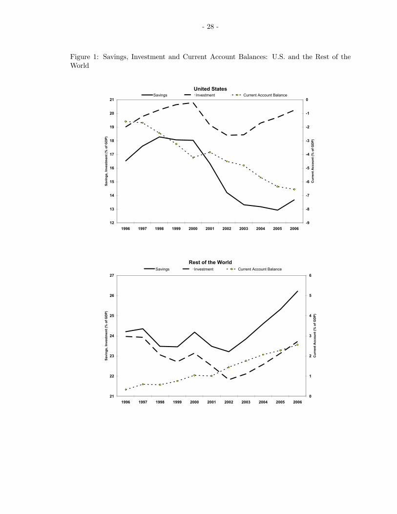
- 28 -

Figure 1: Savings, Investment and Current Account Balances: U.S. and the Rest of theWorld

United States

12

13

14

15

16

17

18

19

20

21

1996 1997 1998 1999 2000 2001 2002 2003 2004 2005 2006

Savi

ngs,

Inve

stm

ent (

% o

f GD

P)

-9

-8

-7

-6

-5

-4

-3

-2

-1

0

Cur

rent

Acc

ount

(% o

f GD

P)

Savings Investment Current Account Balance

Rest of the World

21

22

23

24

25

26

27

1996 1997 1998 1999 2000 2001 2002 2003 2004 2005 2006

Savi

ngs,

Inve

stm

ent (

% o

f GD

P)

0

1

2

3

4

5

6

Cur

rent

Acc

ount

(% o

f GD

P)

Savings Investment Current Account Balance

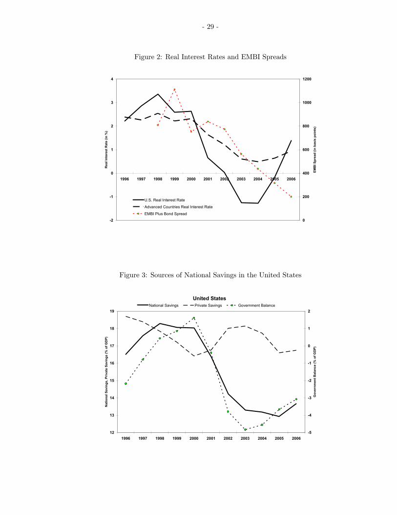
- 29 -

Figure 2: Real Interest Rates and EMBI Spreads

-2

-1

0

1

2

3

4

1996 1997 1998 1999 2000 2001 2002 2003 2004 2005 2006

Rea

l Int

eres

t Rat

e (in

%)

0

200

400

600

800

1000

1200

EMB

I Spr

ead

(in b

asis

poi

nts)

U.S. Real Interest Rate

Advanced Countries Real Interest Rate

EMBI Plus Bond Spread

Figure 3: Sources of National Savings in the United States

United States

12

13

14

15

16

17

18

19

1996 1997 1998 1999 2000 2001 2002 2003 2004 2005 2006

Nat

iona

l Sav

ings

, Priv

ate

Savi

ngs

(% o

f GD

P)

-5

-4

-3

-2

-1

0

1

2G

over

nmen

t Bal

ance

(% o

f GD

P)

National Savings Private Savings Government Balance

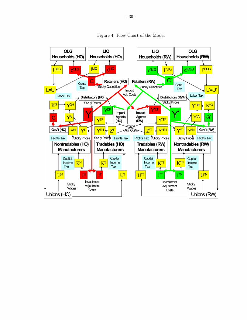
- 30 -

Figure 4: Flow Chart of the Model

OLGHouseholds (HO)

OLGHouseholds (RW)

LIQHouseholds (HO)

LIQHouseholds (RW)

lOLG lLIQ

L=U

Unions (HO)

cOLG cLIQ

Distributors (HO)

C

Y

Nontradables (HO)Manufacturers

Tradables (HO)Manufacturers

YN ZT

YTF

YT

IN IT

KTKN

UN UT

G

Gov’t (HO)

Labor Tax

Cons.Tax

Profits Tax Profits Tax

CapitalIncomeTax

CapitalIncomeTax

ImportAdj. Costs

InvestmentAdjustment

Costs

Sticky Prices Sticky Prices

Sticky Wages

Unions (RW)

L*=U*

l*OLGc*OLGl*LIQc*LIQ

C*

Y*

U*T U*N

Tradables (RW)Manufacturers

Nontradables (RW)Manufacturers

I*NI*T

K*T K*N

InvestmentAdjustment

Costs

CapitalIncomeTax

CapitalIncomeTax

Sticky Wages

Z*T Y*N

Y*TF

Y*T

Distributors (RW)

Sticky Prices Sticky PricesProfits Tax Profits Tax

Retailers (HO) Retailers (RW)Sticky Quantities

Labor Tax

Cons.Tax

KG

YTH Y*TH Gov’t (RW)

G*

K*G

Sticky Quantities

YA

YDH

YDF

Sticky Prices

ImportAgents(HO)

ImportAgents(RW)

Y*A

Y*DF

ImportAdj. Costs

Y*DHSticky Prices

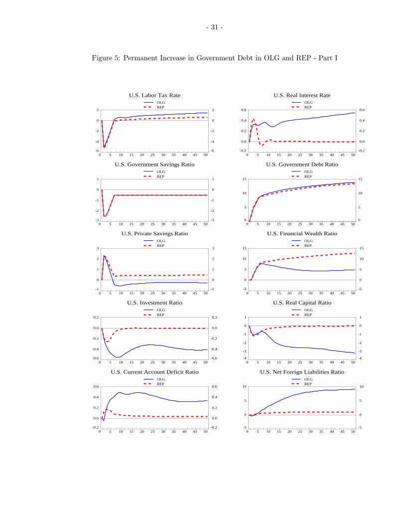
- 31 -

Figure 5: Permanent Increase in Government Debt in OLG and REP - Part I

-6

-4

-2

0

2

-6

-4

-2

0

2

0 5 10 15 20 25 30 35 40 45 50

OLGREP

U.S. Labor Tax Rate

-0.2

0.0

0.2

0.4

0.6

-0.2

0.0

0.2

0.4

0.6

0 5 10 15 20 25 30 35 40 45 50

OLGREP

U.S. Real Interest Rate

-3

-2

-1

0

1

-3

-2

-1

0

1

0 5 10 15 20 25 30 35 40 45 50

OLGREP

U.S. Government Savings Ratio

0

5

10

15

0

5

10

15

0 5 10 15 20 25 30 35 40 45 50

OLGREP

U.S. Government Debt Ratio

-1

0

1

2

3

-1

0

1

2

3

0 5 10 15 20 25 30 35 40 45 50

OLGREP

U.S. Private Savings Ratio

-5

0

5

10

15

-5

0

5

10

15

0 5 10 15 20 25 30 35 40 45 50

OLGREP

U.S. Financial Wealth Ratio

-0.6

-0.4

-0.2

0.0

0.2

-0.6

-0.4

-0.2

0.0

0.2

0 5 10 15 20 25 30 35 40 45 50

OLGREP

U.S. Investment Ratio

-4

-3

-2

-1

0

1

-4

-3

-2

-1

0

1

0 5 10 15 20 25 30 35 40 45 50

OLGREP

U.S. Real Capital Ratio

-0.2

0.0

0.2

0.4

0.6

-0.2

0.0

0.2

0.4

0.6

0 5 10 15 20 25 30 35 40 45 50

OLGREP

U.S. Current Account Deficit Ratio

-5

0

5

10

-5

0

5

10

0 5 10 15 20 25 30 35 40 45 50

OLGREP

U.S. Net Foreign Liabilities Ratio

- 32 -

Figure 6: Permanent Increase in Government Debt in OLG and REP - Part II

-3

-2

-1

0

1

-3

-2

-1

0

1

0 5 10 15 20 25 30 35 40 45 50

OLGREP

U.S. GDP

-3

-2

-1

0

1

-3

-2

-1

0

1

0 5 10 15 20 25 30 35 40 45 50

OLGREP

RW GDP

-4

-2

0

2

-4

-2

0

2

0 5 10 15 20 25 30 35 40 45 50

OLGREP

U.S. Consumption

-2.0

-1.5

-1.0

-0.5

0.0

0.5

-2.0

-1.5

-1.0

-0.5

0.0

0.5

0 5 10 15 20 25 30 35 40 45 50

OLGREP

RW Consumption

-6

-4

-2

0

2

-6

-4

-2

0

2

0 5 10 15 20 25 30 35 40 45 50

OLGREP

U.S. Investment

-0.2

0.0

0.2

0.4

0.6

-0.2

0.0

0.2

0.4

0.6

0 5 10 15 20 25 30 35 40 45 50

OLGREP

U.S. Nominal Interest Rate

-2.0

-1.5

-1.0

-0.5

0.0

0.5

-2.0

-1.5

-1.0

-0.5

0.0

0.5

0 5 10 15 20 25 30 35 40 45 50

OLGREP

U.S. Exports

-0.05

0.00

0.05

0.10

0.15

-0.05

0.00

0.05

0.10

0.15

0 5 10 15 20 25 30 35 40 45 50

OLGREP

U.S. Inflation

-6

-4

-2

0

2

-6

-4

-2

0

2

0 5 10 15 20 25 30 35 40 45 50

OLGREP

U.S. Imports

-3

-2

-1

0

1

2

-3

-2

-1

0

1

2

0 5 10 15 20 25 30 35 40 45 50

OLGREP

U.S. Real Exchange Rate (+ Depreciation)

- 33 -

Figure 7: Cuts in Government Investment and Consumption

-2

-1

0

1

2

-2

-1

0

1

2

0 5 10 15 20 25 30 35 40 45 50

Reduction in Government Investment in the U.S.Reduction in Government Consumption in the U.S.

U.S. GDP

-0.1

0.0

0.1

0.2

0.3

-0.1

0.0

0.1

0.2

0.3

0 5 10 15 20 25 30 35 40 45 50

Reduction in Government Investment in the U.S.Reduction in Government Consumption in the U.S.

RW GDP

-2

0

2

4

-2

0

2

4

0 5 10 15 20 25 30 35 40 45 50

Reduction in Government Investment in the U.S.Reduction in Government Consumption in the U.S.

U.S. Consumption

-0.1

0.0

0.1

0.2

0.3

-0.1

0.0

0.1

0.2

0.3

0 5 10 15 20 25 30 35 40 45 50

Reduction in Government Investment in the U.S.Reduction in Government Consumption in the U.S.

RW Consumption

-2

-1

0

1

2

-2

-1

0

1

2

0 5 10 15 20 25 30 35 40 45 50

Reduction in Government Investment in the U.S.Reduction in Government Consumption in the U.S.

U.S. Investment

-0.4

-0.2

0.0

0.2

0.4

-0.4

-0.2

0.0

0.2

0.4

0 5 10 15 20 25 30 35 40 45 50

Reduction in Government Investment in the U.S.Reduction in Government Consumption in the U.S.

U.S. Nominal Interest Rate

-1.0

-0.5

0.0

0.5

1.0

-1.0

-0.5

0.0

0.5

1.0

0 5 10 15 20 25 30 35 40 45 50

Reduction in Government Investment in the U.S.Reduction in Government Consumption in the U.S.

U.S. Exports

-0.10

-0.05

0.00

0.05

0.10

-0.10

-0.05

0.00

0.05

0.10

0 5 10 15 20 25 30 35 40 45 50

Reduction in Government Investment in the U.S.Reduction in Government Consumption in the U.S.

U.S. Inflation

-0.5

0.0

0.5

1.0

-0.5

0.0

0.5

1.0

0 5 10 15 20 25 30 35 40 45 50

Reduction in Government Investment in the U.S.Reduction in Government Consumption in the U.S.

U.S. Imports

-1.5

-1.0

-0.5

0.0

0.5

1.0

-1.5

-1.0

-0.5

0.0

0.5

1.0

0 5 10 15 20 25 30 35 40 45 50

Reduction in Government Investment in the U.S.Reduction in Government Consumption in the U.S.

U.S. Real Exchange Rate (+ Depreciation)

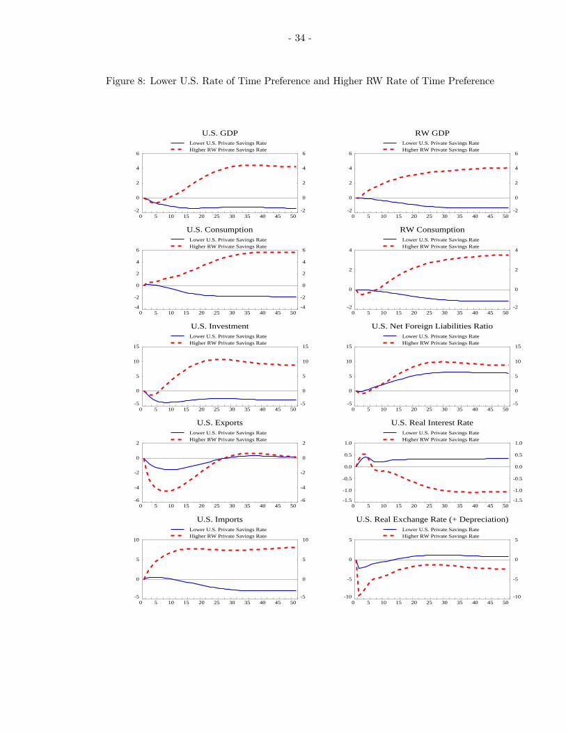
- 34 -

Figure 8: Lower U.S. Rate of Time Preference and Higher RW Rate of Time Preference

-2

0

2

4

6

-2

0

2

4

6

0 5 10 15 20 25 30 35 40 45 50

Lower U.S. Private Savings RateHigher RW Private Savings Rate

U.S. GDP

-2

0

2

4

6

-2

0

2

4

6

0 5 10 15 20 25 30 35 40 45 50

Lower U.S. Private Savings RateHigher RW Private Savings Rate

RW GDP

-4

-2

0

2

4

6

-4

-2

0

2

4

6

0 5 10 15 20 25 30 35 40 45 50

Lower U.S. Private Savings RateHigher RW Private Savings Rate

U.S. Consumption

-2

0

2

4

-2

0

2

4

0 5 10 15 20 25 30 35 40 45 50

Lower U.S. Private Savings RateHigher RW Private Savings Rate

RW Consumption

-5

0

5

10

15

-5

0

5

10

15

0 5 10 15 20 25 30 35 40 45 50

Lower U.S. Private Savings RateHigher RW Private Savings Rate

U.S. Investment

-5

0

5

10

15

-5

0

5

10

15

0 5 10 15 20 25 30 35 40 45 50

Lower U.S. Private Savings RateHigher RW Private Savings Rate

U.S. Net Foreign Liabilities Ratio

-6

-4

-2

0

2

-6

-4

-2

0

2

0 5 10 15 20 25 30 35 40 45 50

Lower U.S. Private Savings RateHigher RW Private Savings Rate

U.S. Exports

-1.5

-1.0

-0.5

0.0

0.5

1.0

-1.5

-1.0

-0.5

0.0

0.5

1.0

0 5 10 15 20 25 30 35 40 45 50

Lower U.S. Private Savings RateHigher RW Private Savings Rate

U.S. Real Interest Rate

-5

0

5

10

-5

0

5

10

0 5 10 15 20 25 30 35 40 45 50

Lower U.S. Private Savings RateHigher RW Private Savings Rate

U.S. Imports

-10

-5

0

5

-10

-5

0

5

0 5 10 15 20 25 30 35 40 45 50

Lower U.S. Private Savings RateHigher RW Private Savings Rate

U.S. Real Exchange Rate (+ Depreciation)

- 35 -

References

Aschauer, D.A. (1989), “Does Public Capital Crowd Out Private Capital?”, Journal ofMonetary Economics, 24, 171-188.

Aschauer, D.A. (1998), “How Big Should the Public Capital Stock Be?”, Jerome LevyInstitute, Policy Brief No. 43.

Bayoumi, T. and Sgherri, S. (2006), “Mr. Ricardo’s Great Adventure: Estimating FiscalMultipliers in a Truly Intertemporal Model”, IMF Working Paper Series,WP/06/168.

Bernanke, B. (2005), “The Global Saving Glut and the U.S. Current Account Deficit”,March 15 speech, available at http:// www.federalreserve.gov/ boarddocs/ speeches/2005/.

Betts, C. and Devereux, M. (2001), “The International Monetary Transmission ofMonetary and Fiscal Policies in a Two-Country Model”, in: M. Obstfeld and G.Calvo, eds., Essays in Honor of Robert A. Mundell. Cambridge: MIT Press.

Blanchard, O.J. (1985), “Debt, Deficits, and Finite Horizons”, Journal of PoliticalEconomy, 93, 223-247.

Blanchard, O.J. and Perotti, R. (2002), “An Empirical Characterization of the DynamicEffects of Changes in Government Spending and Taxes on Output”, QuarterlyJournal of Economics, 117 (4), 1329-1368.

Buiter, W.H. (1981), “Time Preference and International Lending and Borrowing in anOverlapping-Generations Model”, Journal of Political Economy, 89, 769-797.

Caselli, P. (2001), “Fiscal Consolidation Under Fixed Exchange Rates”, EuropeanEconomic Review, 45 (3), 425-450.

Chang, Y. and Kim, S.-B. (2005), “On the Aggregate Labor Supply”, Federal ReserveBank of Richmond Economic Quarterly, 91(1), 21-37.

Chinn, M., 2005, “Getting Serious about theTwin Deficits”,Council on Foreign Relations,Special Council Report No. 10.

Chinn, M. and Ito, H., 2005, “Current Account Balances, Financial Development andInstitutions: Assaying the World ‘Savings Glut’”,NBER Working Paper No. 11761.

Chinn, M. and Lee, J., 2005, “Three Current Acount Balances: A ‘Semi-Structuralist’Interpretation”, NBER Working Paper No. 11853.

Chinn, M. and Steil, B., 2006, “Why Deficits Matter”, The International EconomyMagazine, Summer, 18—23.

Corsetti, G. and Pesenti, P. (2001), “Welfare and Macroeconomic Interdependence”,Quarterly Journal of Economics, 116, 421-445.

- 36 -

Engen, E.M. and Hubbard, R.G. (2004), “Federal Government Debt and Interest Rates”,NBER Macroeconomics Annual, 19, 83-138.

Erceg, C., Guerrieri, L. and Gust, C. (2005a), “SIGMA: A New Open Economy Modelfor Policy Analysis”, Working Paper, Federal Reserve Board.

Erceg, C., Guerrieri, L. and Gust, C. (2005b), “Expansionary Fiscal Shocks And TheTrade Deficit”, International Finance Discussion Paper 825, Board of Governors ofthe Federal Reserve System.

Faruqee, H., Laxton, D., Muir, D. and Pesenti, P. (2005), “Smooth Landing or Crash?Model-Based Scenarios of Global Current Account Rebalancing”, NBER WorkingPaper No. 11583.

Fatas, A., and Mihov, I. (2001), “The Effects of Fiscal Policy on Consumption andEmployment: Theory and Evidence”, CEPR Discussion Paper 2060.

Ferrero, A. (2006), “Demographic Trends, Fiscal Policy and Trade Deficits”, WorkingPaper, New York University.

Frenkel, J.A., and Razin, A. (1992), Fiscal Policies and the World Economy, SecondEdition. Cambridge: MIT Press.

Gali, J., López-Salido, J.D. and Vallés, J. (2007), “Understanding the Effects ofGovernment Spending on Consumption”, Journal of the European EconomicAssociation, 5(1), 227-270.

Ganelli, G. (2005), “The New Open Economy Macroeconomics of Government Debt”,Journal of International Economics, 65(1), 167-184.

Ganelli, G. (2003), “Useful Government Spending, Direct Crowding-Out and FiscalPolicy Interdependence”, Journal of International Money and Finance, 22 (1),87-103.

Ganelli, G., and Lane, P.R. (2002), “Dynamic General Equilibrium Analysis: The OpenEconomy Dimension”, in: S. Altug, J. Chadha, C. Nolan, eds., DynamicMacroeconomic Analysis. Cambridge: Cambridge University Press.

Ghironi, F. (2000a), “Macroeconomic Interdependence Under Incomplete Markets”,Working Paper, Boston College.

Ghironi, F. (2000b), “Understanding Macroeconomic Interdependence: Do We ReallyNeed to Shut Off the Current Account?”, Mimeo, Boston College.

Hooper, P. and Marquez, J. (1995), “Exchange Rates, Prices, and External Adjustmentin the United States and Japan”, in: Kenen, P., ed., Understanding Interdependence,Princeton University Press, Princeton, NJ, 107-168.

Hooper, P., Johnson, K. and Marquez, J. (2000), “Trade Elasticities for the G-7Countries”, Princeton Studies in International Economics, 87.

- 37 -

Ireland, P. (2001), “Sticky-Price Models of the Business Cycle: Specification andStability”, Journal of Monetary Economics, 47, 3-18.

Kamps, C. (2004), “New Estimates of Government Net Capital Stocks for 22 OECDCountries 1960-2001”, IMF Working Paper Series, WP/04/67.

Kopcke, R., Tootell, G. and Triest, R., eds., 2006, The Macroeconomics of Fiscal Policy,Cambridge and London: MIT Press.

Kumhof, M. and Laxton, D. (2006), “How Will Global Imbalances Adjust?”, Box 1.3 ofChapter 1 of the September 2006 IMF World Economic Outlook.

Laubach, T. (2003), “New Evidence on the Interest Rate Effects of Budget Deficits andDebt”, Finance and Economics Discussion Series 2003-12, Board of Governors of theFederal Reserve System.

Laxton, D. and Milesi-Ferretti, G.-M. (2005), “How Will Global Imbalances Adjust?”,Appendix 1.2 of Chapter 1 of the September 2005 IMF World Economic Outlook.

Laxton, D. and Pesenti, P. (2003), “Monetary Rules for Small, Open, EmergingEconomies”, Journal of Monetary Economics, 50(5), 1109-1152.

Ligthart, J.E. and Suárez, R.M.M. (2005), “The Productivity of Public Capital: A MetaAnalysis”, Working Paper, Tilburg University.

Mendoza, E. (2005), “Real Exchange Rate Volatility and the Price of Nontradables inSudden-Stop-Prone Economies”, NBER Working Paper No. 11691.

Obstfeld, M., and Rogoff, K. (1995), “Exchange Rate Dynamics Redux”, Journal ofPolitical Economy, 103, 624-660.

Obstfeld, M., and Rogoff, K. (1996), Foundations of International Macroeconomics.Cambridge: MIT Press.

Orphanides, A. (2003), “Historical Monetary Policy Analysis and the Taylor Rule”,Journal of Monetary Economics, 50, 983-1022.

Pencavel, J. (1986), “Labor Supply of Men”, in: O. Ashenfelter and R. Layards, eds.,Handbook of Labor Economics, Vol. 1. Amsterdam: North Holland.

Straub, R. and Tchakarov, I. (2006), “Assessing the Impact of Change in Composition ofPublic Spending: A DSGE Approach”, Working Paper.

Truman, E., 2006, “Budget and External Deficits: Not Twins but the Same Family,” in:Kopcke, R., Tootell, G. and Triest, R., eds., The Macroeconomics of Fiscal Policy,Cambridge and London: MIT Press.

Weber, C.E. (2002), “Intertemporal Non-Separability and "Rule of Thumb"Consumption”, Journal of Monetary Economics, 49(2), 293-308.

Weil, P. (1989), “Overlapping Families of Infinitely-Lives Agents”, Journal of Public

- 38 -

Economics, 38, 183-198.

Woodford, M. (2003), Interest and Prices: Foundations of a Theory of Monetary Policy.Princeton: Princeton University Press.