A numerical study of Isogeometric Analysisfor cavity flow and flow around a cylindrical

obstacle

Babak S. Hosseini1, Matthias Moller2, and Stefan Turek1

1TU Dortmund, Institute of Applied Mathematics (LS III), Vogelpothsweg 87, 44227 Dortmund,Germany

2Delft University of Technology, Department of Applied Mathematics, Mekelweg 4, 2628 CD Delft,The Netherlands

Abstract

This paper presents our numerical results for the application of the Isogeomet-ric Analysis (IGA) to the velocity-pressure formulation of the steady state as wellas the unsteady incompressible Navier-Stokes equations. For the approximation ofthe velocity and pressure fields, LBB compatible spline spaces are used which canbe regarded as generalizations of Taylor-Hood pairs of finite element spaces. Thesingle-step θ-scheme is used for the discretization in time. The lid-driven cavityflow in addition to its regularized version and flow around cylinder are consideredin two dimensions as model problems in order to investigate the numerical prop-erties of the scheme with respect to accuracy.

Keywords:Isogeometric Analysis; Isogeometric finite elements; B-splines; NURBS; Fluid me-chanics, Navier-Stokes equations, lid-driven cavity flow, flow around cylinder.

1 Introduction

The Isogeometric analysis technique, developed by Hughes et al. [5], is a powerful numer-ical technique aiming to bridge the gap between the worlds of computer-aided engineering(CAE) and computer-aided design (CAD). It unites the benefits of Finite Element Analy-sis (FEA) with the ability of an exact representation of complex computational domainsvia an elegant mathematical description in form of uni-, bi- or trivariate non-uniformrational splines. Non-Uniform Rational B-splines (NURBS) are the de facto industrystandard when it comes to modeling complex geometries, while FEA is a numerical ap-proximation technique, that is widely used in computational mechanics.

1

NURBS and FEA utilize basis functions for the representation of geometry and ap-proximation of field variables, respectively. In order to close the gap between the twotechnologies, Isogeometric Analysis adopts the spline geometry as the computational do-main and utilizes its basis functions to construct both trial and test spaces in the discretevariational formulation of differential problems. The usage of these functions allows theconstruction of approximation spaces exhibiting higher regularity (C≥0) which - depend-ing on the problem to be solved - may be beneficial compared to standard finite elementspaces. In fact, primal variational formulations of high order partial differential equations(PDEs) such as Navier-Stokes-Korteweg (3-rd order spatial derivatives) or Cahn-Hilliard(4-th order spatial derivatives) require piecewise smooth and globally C1 continuous basisfunctions. The number of finite elements possessing C1 continuity and being applicableto complex geometries is already very limited in two dimensions [9, 10]. The Isogeomet-ric Analysis technology features a unique combination of attributes, namely, superioraccuracy on degree of freedom basis, robustness, two- and three-dimensional geometricflexibility, compact support, and the possibility for C≥0 continuity [5].

This article is all about the application and assessment of the Isogeometric Analysisapproach to fluid flows with respect to well known benchmark problems. We present ournumerical results for the lid-driven cavity flow problem (including its regularized version)using different spline approximation spaces and compare them to reference results fromliterature. Despite the fact that investigations of lid-driven cavity type model problemsdo not necessarily reflect the current spirit of time, they are nonetheless a natural firstchoice when its comes to assessing the properties of a numerical scheme.Subsequent to lid-driven cavity, we eventually proceed to present and compare approx-imated physical quantities such as the drag and lift coefficients obtained for the flowaround cylinder benchmark, whereby a multi-patch discretization approach is adopted.For the scenarios addressed, Isogeometric Analysis is applied on the steady-state as wellas transient incompressible Navier-Stokes equations. For the equations under considera-tion are of nonlinear nature, we decided to provide a rather detailed insight concerningtheir treatment. The efficient solution of the discretized system of equations using iter-ative solution techniques such as, e.g., multigrid is not addressed in this paper. Prelim-inary research results are underway and will be presented in a forthcoming publication.In this numerical study, all systems of equations have been solved by a direct solver.

The outline of this paper is as follows. Section 2 is devoted to the introduction ofthe univariate and the multivariate (tensor product) B-spline and NURBS (non-uniformrational B-spline) basis functions, their related spaces and the NURBS geometrical mapF. This presentation is quite brief and notationally oriented. A more complete intro-duction to NURBS and Isogeometric Analysis can be found in [1, 5, 14]. Section 3 isdedicated to the presentation of the governing equations and their variational forms. InSections 4 and 5, numerical results of Isogeometric Analysis of lid-driven cavity flow andflow around cylinder are presented and compared with reference results from literature.

2

2 Preliminaries

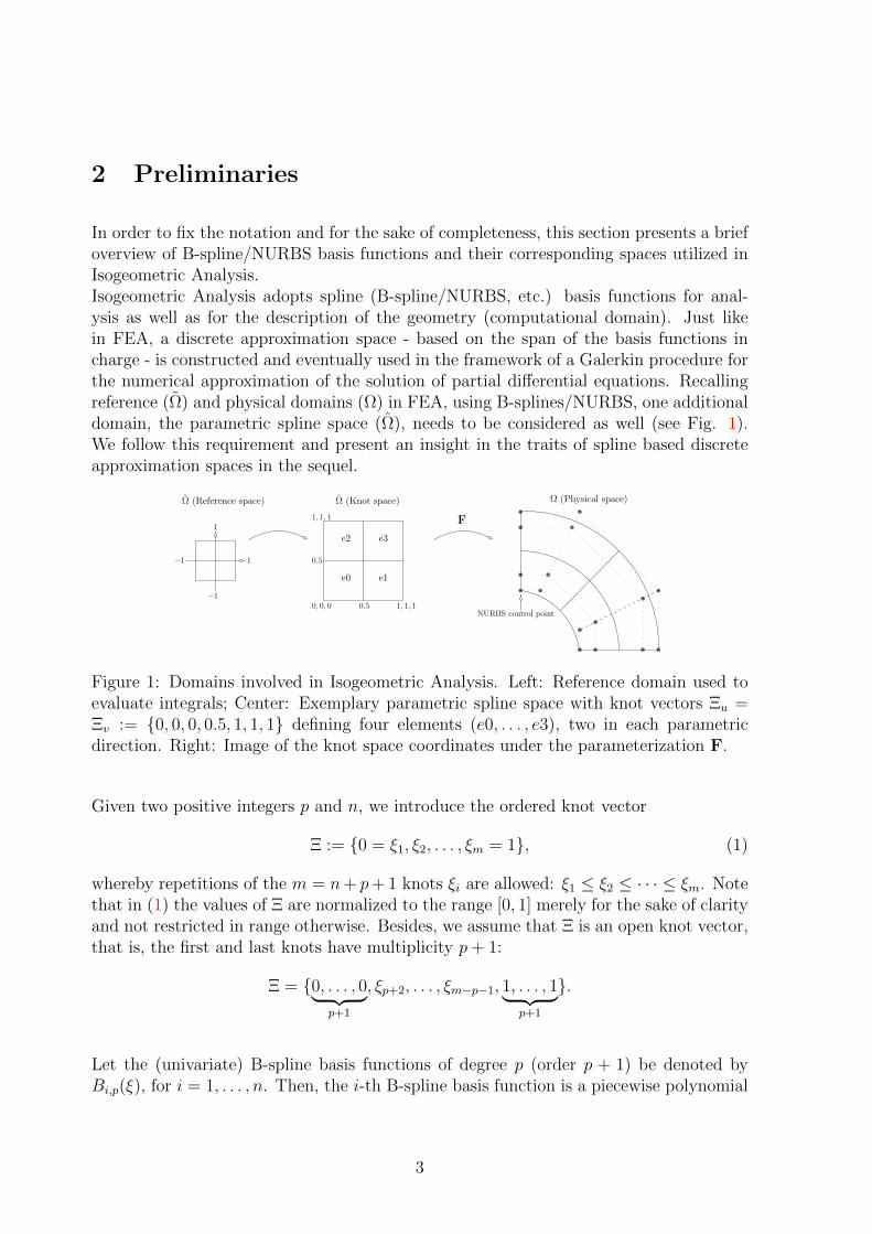
In order to fix the notation and for the sake of completeness, this section presents a briefoverview of B-spline/NURBS basis functions and their corresponding spaces utilized inIsogeometric Analysis.Isogeometric Analysis adopts spline (B-spline/NURBS, etc.) basis functions for anal-ysis as well as for the description of the geometry (computational domain). Just likein FEA, a discrete approximation space - based on the span of the basis functions incharge - is constructed and eventually used in the framework of a Galerkin procedure forthe numerical approximation of the solution of partial differential equations. Recallingreference (Ω) and physical domains (Ω) in FEA, using B-splines/NURBS, one additionaldomain, the parametric spline space (Ω), needs to be considered as well (see Fig. 1).We follow this requirement and present an insight in the traits of spline based discreteapproximation spaces in the sequel.

1

0.5

1, 1, 1

0, 0, 0 0.5

Ω (Knot space)Ω (Reference space)

−1

e0

e2

1

e1

e3

−1

Ω (Physical space)

NURBS control point

F

1, 1, 1

Figure 1: Domains involved in Isogeometric Analysis. Left: Reference domain used toevaluate integrals; Center: Exemplary parametric spline space with knot vectors Ξu =Ξv := 0, 0, 0, 0.5, 1, 1, 1 defining four elements (e0, . . . , e3), two in each parametricdirection. Right: Image of the knot space coordinates under the parameterization F.

Given two positive integers p and n, we introduce the ordered knot vector

Ξ := 0 = ξ1, ξ2, . . . , ξm = 1, (1)

whereby repetitions of the m = n+ p+ 1 knots ξi are allowed: ξ1 ≤ ξ2 ≤ · · · ≤ ξm. Notethat in (1) the values of Ξ are normalized to the range [0, 1] merely for the sake of clarityand not restricted in range otherwise. Besides, we assume that Ξ is an open knot vector,that is, the first and last knots have multiplicity p+ 1:

Ξ = 0, . . . , 0︸ ︷︷ ︸p+1

, ξp+2, . . . , ξm−p−1, 1, . . . , 1︸ ︷︷ ︸p+1

.

Let the (univariate) B-spline basis functions of degree p (order p + 1) be denoted byBi,p(ξ), for i = 1, . . . , n. Then, the i-th B-spline basis function is a piecewise polynomial

3

function and it is recursively defined by the Cox-de Boor recursion formula:

Bi,0(ξ) =

1, if ξi ≤ ξ < ξi+1

0, otherwise

Bi,p(ξ) =ξ − ξiξi+p − ξi

Bi,p−1(ξ) +ξi+p+1 − ξξi+p+1 − ξi+1

Bi+1,p−1(ξ), p > 0.

(2)

At knot ξi the basis functions have α := p− ri continuous derivatives, where ri denotesthe multiplicity of knot ξi. The quantity α is bounded from below and above by −1 ≤α ≤ p − 1. Thus, the maximum multiplicity allowed is ri = p + 1, rendering the basisfunctions at ξi discontinuous as it is the case at the boundaries of the interval.

Each basis function Bi,p is non-negative over its support (ξi, ξi+p+1). The interval (ξi, ξi+1)is referred to as a knot span or element in IGA speak. Moreover, the B-spline basis func-tions are linearly independent and constitute a partition of unity, that is,

∑ni=1 Bi,p(ξ) = 1

for all ξ ∈ [0, 1]. Figure 2 illustrates the basis functions of degree 2 of an exemplary knotvector exhibiting different levels of continuity. Due to the recursive definition (2), the

0

0.2

0.4

0.6

0.8

1

0 0.2 0.4 0.6 0.8 1

B(ξ

)

ξ

B-spline basis functions

B1,2

B2,2 B3,2

B4,2

B5,2B6,2 B7,2

B8,2

Figure 2: Plot of B-spline basis functions of degree 2 corresponding to the open knotvector Ξ := 0, 0, 0, 0.2, 0.4, 0.4, 0.6, 0.8, 1, 1, 1. Due to the open knot vector trait, thefirst and last basis functions are interpolatory, that is, they take the value 1 at thefirst and last knot. At an interior knot ξi the continuity is Cp−ri with ri denoting themultiplicity of knot ξi. Due to the multiplicity r5 = 2 of knot ξ5 = 0.4, the continuityof the basis functions at this parametric point is Cp−2 = C0, while at the other interiorknots the continuity is Cp−1 = C1.

derivative of the i-th B-spline basis function is given by

B′i,p(ξ) =p

ξi+p − ξiBi,p−1(ξ)− p

ξi+p+1 − ξi+1

Bi+1,p−1(ξ) (3)

which is a combination of lower order B-spline functions. The generalization to higherderivatives is straightforward by simply differentiating each side of the above relation.Univariate rational B-spline basis functions are obtained by augmenting the set of B-spline basis functions with weights wi and defining:

Ri,p(ξ) =Bi,p(ξ)wiW (ξ)

, W (ξ) =n∑j=1

Bj,p(ξ)wj. (4)

4

Its derivative is obtained by simply applying the quotient rule. By setting all weightingcoefficients equal to one it follows that B-splines are just a special case of NURBS.

The space of B-splines of degree p and regularity α determined by the knot vector Ξ isspanned by the basis functions Bi,p and will be denoted by

Spα ≡ Spα(Ξ, p) := spanBi,pni=1. (5)

Analogously, we define the space spanned by rational B-spline basis functions as

N pα ≡ N p

α(Ξ, p, w) := spanRi,pni=1. (6)

The definition of univariate B-spline spaces can readily be extended to higher dimen-sions. To this end, we consider d knot vectors Ξβ, 1 ≤ β ≤ d and an open parametricdomain (0, 1)d ∈ Rd. The knot vectors Ξβ partition the parametric domain (0, 1)d intod-dimensional open knot spans, or elements, and thus yield a mesh Q being defined as

Q ≡ Q(Ξ1, . . . ,Ξd) := Q = ⊗dβ=1(ξi,β, ξi+1,β) | Q 6= ∅, 1 ≤ i ≤ mβ (7)

For an element Q ∈ Q, we set hQ = diam(Q), and define the global mesh size h =maxhQ, Q ∈ Q. We define the tensor product B-spline and NURBS basis functions as

Bi1,...,id := Bi1,1 ⊗ · · · ⊗Bid,d, i1 = 1, . . . , n1, id = 1, . . . , nd (8)

andRi1,...,id := Ri1,1 ⊗ · · · ⊗Rid,d, i1 = 1, . . . , n1, id = 1, . . . , nd, (9)

respectively. Then, the tensor product B-spline and NURBS spaces, spanned by therespective basis functions, are defined as

Sp1,...,pdα1,...,αd

≡ Sp1,...,pdα1,...,αd

(Q) := Sp1α1⊗ · · · ⊗ Spdαd

= spanBi1...idn1,...,ndi1=1,...,id=1 (10)

andN p1,...,pdα1,...,αd

≡ N p1,...,pdα1,...,αd

(Q) := N p1α1⊗ · · · ⊗ N pd

αd= spanRi1...id

n1,...,ndi1=1,...,id=1, (11)

respectively. The space Sp1,...,pdα1,...,αd

is fully characterized by the triangulation Q, the degreesp1, . . . , pd of basis functions and their continuities α1, . . . , αd. The minimum regular-ity/continuity of the space is α := minαi, i ∈ (1, d).For a representation of the elements in the physical domain Ω, the triangulation Q ismapped to the physical space via a NURBS geometrical map F : Ω→ Ω

F =

n1∑i1=1

· · ·nd∑id=1

Ri1(ξi1) . . . Rid(ξid)Pi1,...,id (12)

yielding a triangulation K, with

K = F(Q) := F(ξ)|ξ ∈ Q. (13)

5

With the definition of F at hand, the space V of NURBS basis functions on Ω, being thepush-forward of the space N , is defined as

Vp1,...,pdα1,...,αd

≡ Vp1,...,pdα1,...,αd

(K) := Vp1α1⊗ · · · ⊗ Vpdαd

= spanRi1...id F−1n1,...,ndi1=1,...,id=1 (14)

In equation (12), P, denotes a homogeneous NURBS control point uniquely addressedin the NURBS tensor product mesh by its indices.We assume that the parameterization F is invertible, with smooth inverse, on eachelement Q ∈ Q. A mesh stack Qhh≤h0 , with affiliated spaces, can be constructed viaknot insertion as described, e.g., in [5] from an initial coarse mesh Q0, with the globalmesh size h pointing to a refinement level index.

3 Governing equations

For stationary flow scenarios, the governing equations to be solved are the steady-stateincompressible Navier-Stokes equations represented in strong form as

−ν∇2v + (v · ∇)v +∇p = b in Ω (15a)

∇ · v = 0 in Ω (15b)

v = vD on ΓD (15c)

−pv + ν(n · ∇)v = t on ΓN (15d)

where Ω ⊂ R2 is a bounded domain, ρ is the density, µ represents the dynamic viscosity,ν = µ/ρ is the kinematic viscosity, p = P/ρ denotes the normalized pressure, b is thebody force term, vD is the value of the velocity Dirichlet boundary conditions on theDirichlet boundary ΓD, t is the prescribed traction force on the Neumann boundary ΓNand n is the outward unit normal vector on the boundary. The kinematic viscosity andthe density of the fluid are assumed to be constant. The first and second equations in(15) are the momentum and continuity equations, respectively.

Their continuous mixed variational formulation reads:Find v ∈H1

ΓD(Ω) and p ∈ L2(Ω)/R such that,

a(w,v) + c(v;w,v) + b(w, p) = (w, b) + (w, t)ΓN∀w ∈H1

0(Ω)

b(v, q) = 0 ∀q ∈ L2(Ω)/R,(16)

where L2 and H1 are Sobolev spaces as defined in the finite element literature.

Replacement of the linear-, bilinear- and trilinear forms with their respective definitions

6

and application of integration by parts on (16), yields

ν

∫Ω

∇w : ∇v dΩ︸ ︷︷ ︸a(w,v)

+

∫Ω

w · v · ∇v dΩ︸ ︷︷ ︸c(v;w,v)

−∫

Ω

∇ ·wp dΩ︸ ︷︷ ︸b(w,p)

−∫

Ω

q∇ · v dΩ︸ ︷︷ ︸b(v,q)

=

∫Ω

w · b dΩ︸ ︷︷ ︸(w,b)

+

∫∂Ω

νw · (∇v · n) d∂Ω︸ ︷︷ ︸(w,t)ΓN

−∫∂Ω

pw · n, d∂Ω(17)

In addition to the stationary channel flow around a circular obstacle model problem, wealso consider its unsteady counterpart (see Chap. 5). In the latter case, the unsteadyincompressible Navier-Stokes equations, defined as

∂v

∂t− ν∇2v + (v · ∇)v +∇p = b in Ω×]0, T [ (18a)

∇ · v = 0 in Ω×]0, T [ (18b)

v = vD on ΓD×]0, T [ (18c)

−pv + ν(n · ∇)v = t on ΓN×]0, T [ (18d)

v(x, 0) = v0(x) (18e)

are solved in time, whereby the initial condition is required to satisfy ∇ · v0 = 0. Thecorresponding variational problem reads: Find v(x, t) ∈ H1

ΓD(Ω)×]0, T [ and p(x, t) ∈

L2(Ω)×]0, T [, such that for all (w, q) ∈H1Γ0

(Ω)× L2(Ω)/R it holds(w,vt) + a(w,v) + c(v;w,v) + b(w, p) = (w, b) + (w, t)ΓN

b(v, q) = 0(19)

Equations (15) and (18) both have a nonlinear advection term and require techniquesfor the treatment of nonlinear PDEs such as the Newton-Kantorovich method.

3.1 Treatment of Nonlinearity

We will apply Newton’s method being basically a Taylor expansion followed by a lin-earization step. Willing to solve f(x) = 0 (with, e.g., f : R → R ) and having a goodinitial guess for a root, x ≈ x[i], we apply a Taylor expansion of f(x) around x[i] to obtaina power series approximation, given as:

f(x) = f(x[i]) + fx(x[i])(x− x[i]) +O((x− x[i])2) + ... (20)

With a sufficiently good initial guess, one ignores the quadratic and other higher orderterms and obtains the following update formula for x:

x[i+1] = x[i] − f(x[i])/fx(x[i]) (21)

7

Application of Newton’s method on the incompressible steady-state Navier-Stokes equa-tions, requires f to be a functional of the functions to be approximated (velocity andpressure) and fx to be its Gateaux differential. Expressing (17) in operator form

L(v)v = b, (22)

we let f be its (nonlinear) residual w.r.t the current state of the field variables

R(vn−1) := (L(vn−1)vn−1 − b)︸ ︷︷ ︸nonlinear residual

. (23)

It remains to find a representation for fx.The Gateaux differential dF (u;ψ) of F at u ∈ U in the direction ψ ∈ X - being thegeneralization of the concept of the directional derivative - is defined as

dF (u;ψ) = limτ→0

F (u+ τψ)− F (u)

τ=

d

dτF (u+ τψ)

∣∣∣∣τ=0

, (24)

where X and Y are locally convex topological vector spaces, U ⊂ X is open, F : X → Yand the limit exists. Aliasing τψ with u, we express the above term as

F (u+ u) = F (u) + F ′(u)u+O(|u|2) (25)

To derive the Jacobian of L, let it be disassembled as L = LA ⊕ LV ⊕ LG ⊕ LD, withoperators LA = v·∇v, LV = −ν∇2v, LG = ∇p and LD = ∇·v. The Gateaux differentialof the nonlinear operator LA with respect to the direction v, is derived as

L′A(v)v = LA(v + v)− LA(v)

= [(v + v) · ∇(v + v)]− [v · ∇v]

= [[v · ∇(v + v)] + [v · ∇(v + v)]]− [v · ∇v]

= [v · ∇v + v · ∇v + v · ∇v + v · ∇v − v · ∇v]

= [v · ∇v + v · ∇v + v · ∇v]

(26)

The derivatives of the remaining operators LV , LG, and LD can be obtained analogously.Their combination eventually yields

L′(v)v :=

[−ν∇2(·) + (·) · ∇v + v · ∇(·) ∇(·)

∇ · (·) 0

] [vp

]+

[v · ∇v

0

]︸ ︷︷ ︸O(|v|2)→0

(27)

Note that in (27), the symbol (·) denotes the basis functions of the respective perturbationfunctions v =

∑i viϕi and p =

∑i piψi. Their coefficients vi and pi are irrelevant in this

context. With all required ingredients at hand, one nonlinear relaxation step is given by

vn = vn−1 − ωn−1[J(vn−1)]−1 (L(vn−1)vn−1 − b)︸ ︷︷ ︸nonlinear residual

, (28)

where, depending on the complexity to setup and evaluate the Jacobian matrix J , onemay decide to adopt L rather than L′. The scalar quantity ω serves as damping parameterused for tuning and can, e.g., be set to identity.

8

4 Lid-driven cavity flow

The classical driven cavity flow benchmark, considers a fluid in a square cavity. The left,bottom and right walls exhibit no-slip Dirichlet boundary conditions (u = 0), while thetop ”wall” is moved with a constant speed. A schematic representation of the problem

Figure 3: Sketch of lid-driven cavity model.

statement is given in Figure 3. At the upper left and right corners, there is a discontinuityin the velocity boundary conditions producing a singularity in the pressure field at thosecorners. They can either be considered as part of the upper boundary or as part of thevertical walls. The former case, is referred to as the ”leaky” cavity rendering the latter”non-leaky”. For equation (15) involves only the gradient of pressure, we fix the pressuresolution through a Dirichlet boundary condition of 0 at the lower left corner of the cavity.

Our results, obtained with various B-spline space based discretizations, are compared toreference results from the literature such as those of Ghia [8]. Furthermore, additionalcomparisons are done with highly accurate, spectral (Chebyshev Collocation) methodbased solutions of Botella [2] showing convergence up to seven digits.

For an Isogeometric Analysis based approximation of the unknowns in (15), suitableB-spline or NURBS spaces, as defined in Section 2, need to be specified. We usean LBB-stable Taylor-Hood like space pair in the parametric spline domain, whereQTHh ≡ QTH

h (p,α) = Sp1,p2α1,α2

F−1 and VTHh = Sp1+1,p2+1

α1,α2 F−1, are B-spline spaces

for the approximation of pressure and velocity function, respectively [4]. A downcast ofthe variational formulation (16) to the discrete level, gives rise to the problem statement:

Find v ∈H1,hΓD

(Ω) ∩ VTHh and p ∈ Lh2(Ω)/R ∩ QTH

h such that,

a(wh,vh) + c(vh;wh,vh) + b(wh, ph) = (wh, bh) + (wh, th)ΓN∀wh ∈H1,h

0 (Ω) ∩ VTHh

b(vh, qh) = 0 ∀qh ∈ Lh2(Ω)/R ∩ QTHh

(29)with superscript h dubbing the mesh family index.

Using the B-spline space pair S2,20,0 × S

1,10,0 for the approximation of the velocity and

pressure functions, in Figure 4 we present our results for stream function (ψ) and vor-ticity (ω) profiles for Reynolds numbers 100, 400 and 1000. Note that we have not taken

9

any stabilization measures for the advection term. The approach we follow for the com-

Figure 4: Stream function (left) and vorticity (right) profiles for Reynolds 100, 400 and1000 from top to bottom. Respective contour ranges for stream function and vorticity:ψiso ∈ [−10−10, 3× 10−3], ωiso ∈ [−5, 3]. Discretization: S2,2

0,0 ×S1,10,0 . Refinement level: 6.

Number of degrees of freedom: 37507.

putation of the stream function in 2D, is based on solving a Poisson equation for ψ with

10

the scalar 2D vorticity function on the right hand side:

−∇2ψ = ω

ω = ∇× v =∂v

∂x− ∂u

∂y

(30)

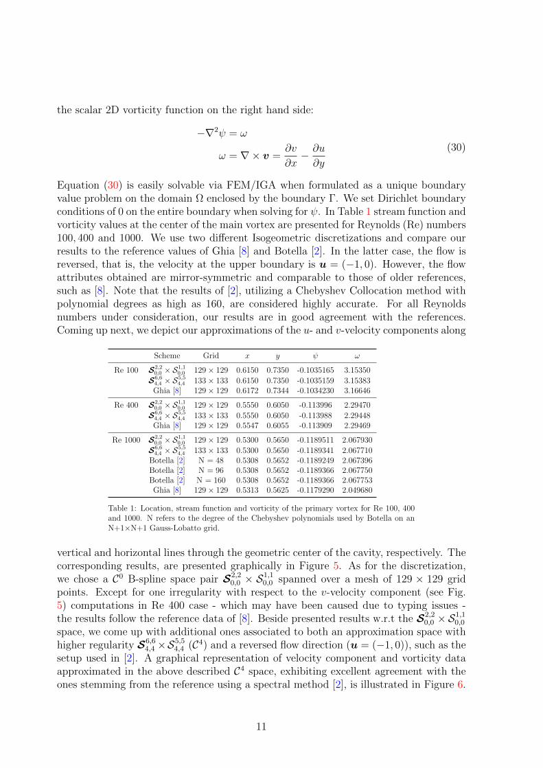
Equation (30) is easily solvable via FEM/IGA when formulated as a unique boundaryvalue problem on the domain Ω enclosed by the boundary Γ. We set Dirichlet boundaryconditions of 0 on the entire boundary when solving for ψ. In Table 1 stream function andvorticity values at the center of the main vortex are presented for Reynolds (Re) numbers100, 400 and 1000. We use two different Isogeometric discretizations and compare ourresults to the reference values of Ghia [8] and Botella [2]. In the latter case, the flow isreversed, that is, the velocity at the upper boundary is u = (−1, 0). However, the flowattributes obtained are mirror-symmetric and comparable to those of older references,such as [8]. Note that the results of [2], utilizing a Chebyshev Collocation method withpolynomial degrees as high as 160, are considered highly accurate. For all Reynoldsnumbers under consideration, our results are in good agreement with the references.Coming up next, we depict our approximations of the u- and v-velocity components along

Scheme Grid x y ψ ω

Re 100 S2,20,0 × S

1,10,0 129× 129 0.6150 0.7350 -0.1035165 3.15350

S6,64,4 × S

5,54,4 133× 133 0.6150 0.7350 -0.1035159 3.15383

Ghia [8] 129× 129 0.6172 0.7344 -0.1034230 3.16646

Re 400 S2,20,0 × S

1,10,0 129× 129 0.5550 0.6050 -0.113996 2.29470

S6,64,4 × S

5,54,4 133× 133 0.5550 0.6050 -0.113988 2.29448

Ghia [8] 129× 129 0.5547 0.6055 -0.113909 2.29469

Re 1000 S2,20,0 × S

1,10,0 129× 129 0.5300 0.5650 -0.1189511 2.067930

S6,64,4 × S

5,54,4 133× 133 0.5300 0.5650 -0.1189341 2.067710

Botella [2] N = 48 0.5308 0.5652 -0.1189249 2.067396Botella [2] N = 96 0.5308 0.5652 -0.1189366 2.067750Botella [2] N = 160 0.5308 0.5652 -0.1189366 2.067753Ghia [8] 129× 129 0.5313 0.5625 -0.1179290 2.049680

Table 1: Location, stream function and vorticity of the primary vortex for Re 100, 400and 1000. N refers to the degree of the Chebyshev polynomials used by Botella on anN+1×N+1 Gauss-Lobatto grid.

vertical and horizontal lines through the geometric center of the cavity, respectively. Thecorresponding results, are presented graphically in Figure 5. As for the discretization,we chose a C0 B-spline space pair S2,2

0,0 × S1,10,0 spanned over a mesh of 129 × 129 grid

points. Except for one irregularity with respect to the v-velocity component (see Fig.5) computations in Re 400 case - which may have been caused due to typing issues -the results follow the reference data of [8]. Beside presented results w.r.t the S2,2

0,0 ×S1,10,0

space, we come up with additional ones associated to both an approximation space withhigher regularity S6,6

4,4 ×S5,54,4 (C4) and a reversed flow direction (u = (−1, 0)), such as the

setup used in [2]. A graphical representation of velocity component and vorticity dataapproximated in the above described C4 space, exhibiting excellent agreement with theones stemming from the reference using a spectral method [2], is illustrated in Figure 6.

11

-0.6

-0.5

-0.4

-0.3

-0.2

-0.1

0

0.1

0.2

0.3

0.4

0 0.2 0.4 0.6 0.8 1

v

x

v-velocity over x

Present Re 100Ghia Re 100

Present Re 400Ghia Re 400

Present Re 1000Ghia Re 1000

0

0.2

0.4

0.6

0.8

1

-0.4 -0.2 0 0.2 0.4 0.6 0.8 1

y

u

u-velocity over y

Present Re 100Ghia Re 100

Present Re 400Ghia Re 400

Present Re 1000Ghia Re 1000

Figure 5: Profiles of v- and u-velocity components over horizontal and vertical linesthrough geometric center of the cavity for Re 100, 400 and 1000. Discretization: S2,2

0,0 ×S1,1

0,0 ; 129× 129 grid points.

4.1 Regularized driven cavity flow

In the regularized lid-driven cavity flow scenario [3], the flow domain is a unit squareexhibiting no-slip Dirichlet boundary conditions at the vertical and lower horizontalboundaries. In a standard lid-driven cavity flow setup, the velocity at the top boundaryis taken to be constant leading to pressure singularities in the upper left and right domaincorners. In order to avoid the singularities, the regularized lid-driven cavity flow problemdefines the following velocity profile on the top boundary

ulid = [−16x2(1− x)2, 0] (31)

Fixing the pressure at the lower left domain node with p = 0, we compute the globalquantities kinetic energy (E) and enstrophy (Z)

E =1

2

∫Ω

‖u‖2 dx, Z =1

2

∫Ω

‖ω‖2 dx, (32)

where ω = ∂v∂x− ∂u

∂ydenotes the vorticity.

In Table 2 we compare our results for Reynolds number 1000 to those published in [3]and [13]. All three isogeometric finite element pairs in charge produced very satisfactoryresults for kinetic energy and enstrophy obviously well integrating with references.

12

-0.6-0.5-0.4-0.3-0.2-0.1

00.10.20.30.4

0 0.2 0.4 0.6 0.8 1

v

x

v-velocity over x

PresentBotella N160

0

0.2

0.4

0.6

0.8

1

-1 -0.8 -0.6 -0.4 -0.2 0 0.2 0.4

y

u

u-velocity over y

PresentBotella N160

-10

-8

-6

-4

-2

0

2

4

0 0.2 0.4 0.6 0.8 1

ω

x

Vorticity over x

PresentBotella N160

0

0.2

0.4

0.6

0.8

1

-6 -4 -2 0 2 4 6 8 10 12 14 16

y

ω

Vorticity over y

PresentBotella N160

Figure 6: Profiles of v- and u-velocity components and vorticity over horizontal andvertical lines through geometric center of the cavity for Re 1000. Discretization: S6,6

4,4 ×S5,5

4,4 ; 133× 133 grid points.

5 Flow around cylinder

Flow around an obstacle in a channel, is a prominent configuration for the assessmentof flow affiliated attributes, produced by a numerical technique in charge with the anal-ysis. Placing our focus on the classical flow around a circular obstacle benchmark, thecomputational scenario follows the lines of [7, 12, 15] and defines the underlying ge-ometry as a pipe where a circular cylinder of radius r = 0.05 has been cut out, thatis, Ω = [0, 2.2] × [0, 0.41] \ Br(0.2, 0.2). The fluid density and kinematic viscosity aretaken as ρ = 1 and ν = 0.001. We require no-slip boundary conditions for the lowerand upper walls Γ1 = [0, 2.2] × 0 and Γ3 = [0, 2.2] × 0.41 as well as the bound-ary S = ∂Br(0.2, 0.2): u|Γ1 = u|Γ3 = u|S = 0. On the left edge Γ4 = 0 × [0, 0.41], a

parabolic inflow profile is prescribed, u(0, y) =(

4Uy(0.41−y)0.412 , 0

), with a maximum velocity

U = 0.3. On the right edge Γ4 = 2.2× [0, 0.41], do-nothing boundary conditions definethe outflow, ν∂ηu − pη = 0 with η denoting the outer normal vector. For a maximum

13

Scheme Grid(points) Kinetic Energy Enstrophy Elements Level

S2,20,0 × S

1,10,0 65× 65 0.022909 4.80747 32× 32 L5

129× 129 0.022778 4.82950 64× 64 L6257× 257 0.022767 4.83041 128× 128 L7513× 513 0.022767 4.83043 256× 256 L8

S3,30,0 × S

2,20,0 49× 49 0.022905 4.81717 16× 16 L4

97× 97 0.022773 4.83079 32× 32 L5193× 193 0.022767 4.83047 64× 64 L6385× 385 0.022767 4.83042 128× 128 L7

S3,31,1 × S

2,21,1 66× 66 0.022777 4.82954 32× 32 L5

130× 130 0.022767 4.83048 64× 64 L6258× 258 0.022767 4.83046 128× 128 L7

Ref. [3] (Bruneau ) 64× 64 0.021564 4.6458128× 128 0.022315 4.7711256× 256 0.022542 4.8123512× 512 0.022607 4.8243

Ref. [13] (Q2P1) 64× 64 0.022778 4.82954128× 128 0.022768 4.83040256× 256 0.022766 4.83050

Table 2: Kinetic energy and enstrophy of the regularized cavity flow for Reynolds 1000.

velocity of U = 0.3, the parabolic profile results in a mean velocity U = 23· 0.3 = 0.2.

The flow configurations characteristic length is D = 2 · 0.05 = 0.1 the diameter of theobject perpendicular to the flow direction. This particular problem configuration yieldsReynolds number Re = UD

ν= 0.2·0.1

0.001= 20 for which the flow is considered stationary.

Following the above setup for Re = 20, we present the results of the application ofIsogeometric Analysis with a special emphasis on approximated drag and lift valuesrelated to the entire obstacle boundary.With S dubbing the surface of the obstacle, nS its inward pointing unit normal vectorw.r.t. the computational domain Ω, tangent vector τ := (ny,−nx)T and uτ := u · τ , thedrag and lift forces are given by

Fdrag =

∫S

(ρν∂uτ∂nS

ny − pnx)ds, Flift = −

∫S

(ρν∂uτ∂nS

nx − pny)ds

Cdrag =2

ρU2DHFdrag, Clift =

2

ρU2DHFlift,

(33)

where u, p and H, represent velocity, pressure and channel height, respectively [11]. Wefollow, however, the alternative approach of [11, 16] and evaluate a volume integral forthe approximations of the drag and lift coefficients. Given filter functions

vd|S = (1, 0)T ,vd|Ω−S = 0 vl|S = (0, 1)T ,vl|Ω−S = 0, (34)

the corresponding volume integral expressions read

Cdrag = − 2

ρU2DH[(ν∇u,∇vd)− (p,∇ · vd)]

Clift = − 2

ρU2DH[(ν∇u,∇vl)− (p,∇ · vl)]

(35)

14

with (·, ·) denoting the L2(Ω) inner product.

We model the computational domain as a multi-patch NURBS mesh (see Fig. 7), sincethe parametric space of a multi-variate NURBS patch exhibits a tensor product struc-ture, and thus, is not mappable to any other topology than a cube in the respectiveN -dimensional space. However, the multi-patch setup yields a perfect mathematicalrepresentation of the circular boundary and in particular avoids its approximation withstraight line segments. Note that each quarter of the “obstacle circle” can be modeledexactly with a NURBS curve of degree 2 and just 3 control points. Since the abilityto exactly represent conical sections is restricted to rational B-splines only, a NURBSmesh came in handy for modeling of the computational domain. With the degrees of

Figure 7: Multi-patch NURBS domain for flow around cylinder. Each uniquely coloredinitial 1× 1 element patch has been refined three times, giving rise to 8× 8 elements ineach patch, eventually.

freedom being defined on the NURBS control points, and the latter failing to have astraightforward and obvious association to a distinct position on the physical mesh, thequestion arises how to set up the inflow boundary condition on the control points tofinally obtain a parabolic inflow profile. We performed a finite element L2-projection∫

Ω

(f − Phf) w dΩ = 0, ∀w ∈ Wh (36)

of the inflow profile f on the control points associated with the left boundary in Fig. 7,whereby Wh denotes a suitable discrete space of weighting/test functions.

Our results for drag, lift and pressure drop, evidently showing good agreement withthe reference, are depicted alongside reference values in Table 3.

Comparing the presented C0 and C1 IGA based discretizations, one observes in the lattercase a reduced amount of degrees of freedom on the same number of elements, whichis due to the extended support of the respective basis functions. This leads on meshrefinement levels ≥ 1 to numbers of degrees of freedom which are not well comparablebetween the two IGA based discretizations. However, a linear interpolation of the dragand lift coefficients, as depicted in Figure 8, delineates the accuracy wise superiorityof the high continuity C1 approach. The semantics of superiority is in terms of gainedaccuracy with respect to the number of degrees of freedom invested. However, for thesake of a fair evaluation, we point out that approximation in high degree and regularity

15

5.56

5.58

5.6

5.62

5.64

5.66

5.68

5.7

5.72

0 20000 40000 60000 80000 100000 120000 140000

dra

g

dofs

ref

S3,30,0 × S

2,20,0

S3,31,1 × S

2,21,1

0.006

0.007

0.008

0.009

0.01

0.011

0.012

0.013

0.014

0 20000 40000 60000 80000 100000120000140000

lift

dofs

ref

S3,30,0 × S

2,20,0

S3,31,1 × S

2,21,1

Figure 8: Drag and lift approximation results compared to reference [7]. Discretizations:S3,3

0,0 × S2,20,0 ; S3,3

1,1 × S2,21,1

spaces, comes at a cost of more expensive cubature rules reflecting the basis functiondegrees (#cub.pts. = p + 1), and the evaluation of high degree, thus more expensive,spline basis functions. Moreover, as the supports of the basis functions extend with risingregularities, so do the couplings among the degrees of freedom. This contributes to agreater matrix fill-in and may increase the burden on the shoulders of existing solutionmethods for sparse linear system of equations.

It should be noted that the solutions we obtained with the C>0 approaches still re-duce to C0 at patch boundaries. There exist means to overcome this deficiency [5], noneof them have been considered in this study, though.

Scheme Cdrag Clift ∆p Degrees of freedom Elements Level

S3,30,0 × S

2,20,0 6.87638 0.102597 0.206858 180 6 L0

S3,30,0 × S

2,20,0 5.66806 0.031363 0.118502 624 24 L1

S3,30,0 × S

2,20,0 5.71406 0.010623 0.116011 2304 96 L2

S3,30,0 × S

2,20,0 5.64576 0.006755 0.116750 8832 384 L3

S3,30,0 × S

2,20,0 5.59464 0.009499 0.117328 34560 1536 L4

S3,30,0 × S

2,20,0 5.58212 0.010407 0.117490 136704 6144 L5

S3,30,0 × S

2,20,0 5.57992 0.010586 0.117516 543744 24576 L6

S3,31,1 × S

2,21,1 6.87638 0.102597 0.206858 180 6 L0

S3,31,1 × S

2,21,1 5.76865 0.011653 0.112236 432 24 L1

S3,31,1 × S

2,21,1 5.68962 0.013130 0.115025 1260 96 L2

S3,31,1 × S

2,21,1 5.64735 0.006661 0.116317 4212 384 L3

S3,31,1 × S

2,21,1 5.59476 0.009502 0.117224 15300 1536 L4

S3,31,1 × S

2,21,1 5.58215 0.010408 0.117489 58212 6144 L5

Ref. [7, 12] 5.57953523384 0.010618948146 0.11752016697

Table 3: Approximation results for drag, lift and pressure drop (∆p).

In the following we turn our attention to the time periodic dfg flow around cylin-der benchmark for re 100, as described in [6, 15]. Here the maximum velocity of

the parabolic inflow profile amounts to U = 1.5, yielding Re = UDν

=23· 32·0.1

0.001= 100. In

order to obtain a time profile for the drag and lift quantities, Isogeometric Analysis was

16

applied on the unsteady incompressible Navier-Stokes equations (18) using the B-splinespaces QTH

h = S2,20,0 F−1 and VTH

h = S3,30,0 F−1 for pressure and velocity, respectively.

This corresponds to solving the system in a fully coupled manner since we solve for allunknown functions simultaneously.

The semi-discretized counterpart of the variational formulation (19) reads:Find v ∈H1,h

ΓD(Ω) ∩ VTH

h ×]0, T [ and p ∈ Lh2(Ω)/R ∩ QTHh ×]0, T [ such that,

∀wh ∈H1,h0 (Ω) ∩ VTH

h and ∀qh ∈ Lh2(Ω)/R ∩ QTHh

(wh,vht ) + a(wh,vh) + c(vh;wh,vh) + b(wh, ph) = (wh, bh) + (wh, th)ΓN

b(vh, qh) = 0

(37)

For the time discretization, the single step θ-scheme with θ = 0.5 is used, leading tothe 2-nd order accurate implicit Crank-Nicolson scheme [17]. Together with the spacediscretization the following nonlinear block system has to be solved in every time step.(

1∆t

M + θ(D + C(vn+1)) GGT 0

)(vn+1

pn+1

)=

(1

∆tM− (1− θ)(D + C(vn)) 0

0 0

)(vn

pn

)+ θfn+1 + (1− θ)fn

(38)In the above system, M,D,C,G and GT denote the mass, diffusion, advection, gradientand divergence matrices, respectively. The body forces are discretized into f .An exemplary sectional view of the approximated lift time profile is presented in Fig-ure 9. Our results are plotted alongside those obtained from [6] using Q2/P

disc1 finite

elements (without stabilization) for space discretization and Crank-Nicolson scheme fortime discretization. All computations performed, are based on the NURBS mesh de-picted in Figure 7. Note that it substantially differs from that used in [6] in terms ofstructure and number of degrees of freedom. In fact, our mesh has roughly 18% lessdegrees of freedom on each level as can be seen from Table 4. For all mesh levels we

Level #DOFs NURBS mesh (7) #DOFs reference mesh ([6]) Ratio

L3 8832 10608 ∼ 8/10L4 34560 42016 ∼ 8/10L5 136704 167232 ∼ 8/10

Table 4: Comparison of the number of degrees of freedom per level

performed an intermediate computation with a very coarse time step (∆t = 1/10) fora total time of 35 simulation seconds. This yielded a profile which we took as initialsolution for the final computation with a finer time step, scheduled for 30 simulationseconds. Note that the depicted time interval is chosen arbitrarily after the drag and liftprofiles were considered developed. In addition, the curves have been shifted in time inorder to facilitate comparison. As far as the treatment of nonlinearity is concerned, forevery time step, the nonlinear iteration loop was iterated until the nonlinear residual ofequation (38) was reduced to 10−3 of its initial value. Tables 5 and 6 supply minimum,maximum, mean and amplitude values for the drag and lift coefficients w.r.t differentmesh levels. In addition to min/max drag and lift coefficients, further quantities of

17

-1.00

-0.50

0.00

0.50

1.00

19.05 19.1 19.15 19.2 19.25 19.3 19.35 19.4

t (sec)

0.91

0.92

0.93

0.94

0.95

0.96

0.97

0.98

0.99

19.203 19.214 19.226 19.237 19.248

t (sec)

cpl, L3,∆t = 1/400

cpl, L4,∆t = 1/400

cpl, L5,∆t = 1/400

Ref., L5,∆t = 1/400

cpl, L3,∆t = 1/400

cpl, L4,∆t = 1/400

cpl, L5,∆t = 1/400

Ref., L5,∆t = 1/400

Figure 9: Sectional views of lift time profile.

Level ∆t min(Cdrag) max(Cdrag) mean(Cdrag) amp(Cdrag)

L3 1/400 3.2732 3.3329 3.3031 5.966E-2L4 1/400 3.2218 3.2857 3.2537 6.394E-2L5 1/400 3.1757 3.2392 3.2075 6.354E-2

Table 5: min/max drag coefficient values

Level ∆t min(Clift) max(Clift) mean(Clift) amp(Clift)

L3 1/400 -0.9466 0.92939 -0.00861 1.8760L4 1/400 -1.0302 0.99033 -0.01995 2.0206L5 1/400 -1.0249 0.98903 -0.01794 2.0139

Table 6: min/max lift coefficient values

interest are the lift profile frequency (f) and Strouhal number (St = DfU

) which we pro-vide values for in Table 7. Bearing in mind the significantly smaller number of degrees of

Level ∆t 1/f (present) St (present) 1/f [6] St [6]

L3 1/400 3.2804E-1 0.30484 3.3000E-01 0.30303L4 1/400 3.3154E-1 0.30162 3.3250E-01 0.30075L5 1/400 3.3143E-1 0.30172 3.3000E-01 0.30303

Table 7: Frequency and Strouhal numbers for different mesh levels.

freedom invested (∼ 18% less) for the approximation of the physical quantities of interestand observing a satisfying agreement with results obtained from the alternative numer-ical implementation of [6] using Q2/P

disc1 finite elements, the overall conclusions drawn,

depict Isogeometric Analysis as a robust and powerful tool at hand well applicable toproblems considered in this study.

18

6 Summary and conclusions

Isogeometric Analysis was applied to well known model flow problems in order to inves-tigate its approximation properties and numerical behavior. Starting off with the lid-driven cavity flow problem, including its regularized version, we have shown in Chapter4 that the approximated flow attributes are very well comparable with reference resultspartially obtained with a highly accurate, spectral (Chebyshev Collocation) method [2].Moreover, in Chapter 4.1 we have extended our view to global quantities such as kineticenergy and enstrophy and have provided results which are at least as good as referenceresults obtained with other approaches such as Q2P1 standard finite elements [13] and ahigh order finite difference scheme utilized in [3].

In addition to cavity flow, we chose the prominent flow around cylinder benchmark, pro-posed in [15], to explore the approximation traits of isogeometric finite elements. The us-age of a C1 B-spline element pair, turned out to be superior to its C0 counterpart in termsof the number of degrees of freedom required to gain a certain accuracy. This comes,however, at a cost of more expensive evaluations of higher degree B-spline/NURBS basisfunctions and increased degree of freedom coupling, leading to broader matrix stencils.Thus, care must be taken with claims regarding general superiority of higher continuity(C≥1) approximations.

We eventually turned our attention to the unsteady Re-100 flow around cylinder case in-volving the transient form of the Navier-Stokes equations. The governing equations werediscretized in time with a second order implicit time discretization scheme and finallysolved in a fully coupled mode. Given the fact that the multi-patch NURBS mesh weused (see Fig. 7) is shown to have about 1/5 less degrees of freedom than the referencemesh used in [6, 7, 15], the presented time profiles of the physical quantities drag andlift are satisfactorily.

Isogeometric Analysis proved for us to be a solid and reliable technology showcasingunique features. For Taylor-Hood like B-spline elements we carried our analysis upon,it turned out to be just a matter of changing settings in a configuration file to set up adesired B-spline element of a specific degree and continuity. This is without any doubta huge benefit when compared to usual finite elements where one needs to provide animplementation for each element type. Moreover, for B-spline/NURBS geometries, al-ready exactly representing a computational domain on the coarsest level, the process ofmeshing is entirely pointless. The mathematical definition of a B-spline/NURBS alreadydefines a tensor product mesh eligible to NURBS based refinement techniques such ash-, p- or k-refinement [5, 14].However, on a final note, the true virtue of the technology can be better exploited in ap-plications involving high order partial differential equations such as e.g. the third orderNavier-Stokes-Korteweg [10] or fourth order Cahn-Hilliard equations [9] in combinationwith complex geometries.

19

References

[1] Y. Bazilevs, L. Beirao da Veiga, J.A. Cottrell, T.J.R. Hughes, and G. Sangalli.Isogeometric analysis: Approximation, stability and error estimates for h-refinedmeshes. Math. Models Methods Appl. Sci. 16, 1031, 2006.

[2] O. Botella and R. Peyret. Benchmark spectral results on the lid-driven cavity flow.Computers & Fluids, Volume 27, Issue 4:421–433, 1 May 1998.

[3] Charles-Henri Bruneau and Mazen Saad. The 2d lid-driven cavity problem revisited.Computers & Fluids, 35, Issue 3:326–348, March 2006.

[4] A. Buffa, C. de Falco, and G. Sangalli. Isogeometric analysis: Stable elements for the2D Stokes equation. International Journal for Numerical Methods in Fluids. SpecialIssue: Numerical Methods for Multi-material Fluids and structures, MULTIMAT-2009, 65 Issue 11-12:1407–1422, 20 - 30 April 2011.

[5] J. Austin Cottrell, Thomas J. R. Hughes, and Yuri Bazilevs. Isogeometric Analysis:Toward Integration of CAD and FEA. Wiley; 1 edition (September 15, 2009), 2009.

[6] http://www.featflow.de/en/benchmarks/cfdbenchmarking/flow/dfg_

benchmark2_re100.html [Online; accessed 01-Oct-2014].

[7] http://www.featflow.de/en/benchmarks/cfdbenchmarking/flow/dfg_

benchmark_re20.html [Online; accessed 01-Oct-2014].

[8] U. Ghia, K. N. Ghia, and C.T. Shin. High-Re solutions for incompressible flow usingthe Navier-stokes Equations and a multigrid method. Journal of computationalphysics, 48, Issue 3:387–411, December 1982.

[9] Hector Gomez, Victor M. Calo, Yuri Bazilevs, and Thomas J.R. Hughes. Isogeomet-ric analysis of the Cahn-Hilliard phase-field model. Computer Methods in AppliedMechanics and Engineering., 197, Issues 49–50:4333–4352, 15 September 2008.

[10] Hector Gomez, Thomas J.R. Hughes, Xesus Nogueira, and Victor M. Calo. Iso-geometric analysis of the isothermal Navier-Stokes-Korteweg equations. ComputerMethods in Applied Mechanics and Engineering, 199, Issues 25–28:1828–1840, 15May 2010.

[11] Volker John. Higher order finite element methods and multigrid solvers in a bench-mark problem for the 3D Navier–Stokes equations. International Journal for Nu-merical Methods in Fluids, 40, Issue 6:775–798, 2002.

[12] G. Nabh. On High Order Methods for the Stationary Incompressible Navier-StokesEquations. PhD thesis, University of Heidelberg, 1998.

[13] Masoud Nickaeen, Abderrahim Ouazzi, and Stefan Turek. Newton multigrid least-squares FEM for the V-V-P formulation of the Navier-Stokes equations. Journal ofComputational Physics, 256:416–427, 1 January 2014.

20

[14] Les A. Piegl and Wayne Tiller. The NURBS book. Monographs in visual communi-cation. Springer, 1995.

[15] M. Schafer, S. Turek, F. Durst, E. Krause, and R. Rannacher. Benchmark compu-tations of laminar flow around a cylinder, January 1996.

[16] S. Turek, A. Ouazzi, and J. Hron. On pressure separation algorithms (pSepA) forimproving the accuracy of incompressible flow simulations. International Journalfor Numerical Methods in Fluids, 59, Issue 4:387–403, 2009.

[17] Stefan Turek. Efficient Solvers for Incompressible Flow Problems - An Algorithmicand Computational Approach, volume 6 of Lecture Notes in Computational Scienceand Engineering. Springer, 1999.

21