example: heat ow solving heat ow with an integral … heat ow let us rst solve the heat equation...

Example: Heat flow

Let us first solve the heat equation analytically before discussingthe numerical method to solve it.

Example: Heat equation in one spatial dimension.

∂T

∂t= κ

∂2T

∂x2,

where κ is the thermal diffusivity.

Open boundaries: T (x , t) defined on −∞ < x < +∞ and t ≥ 0.Also, require that T (x , t)→ 0 as x ±∞

Initial value problem: T (x , t = 0) = Φ(x)

We will use the Fourier transform in order to solve this problem.

Solving Heat flow with an integral transform

We have two independent variables x , t. Apply Fourier transformto spatial variables x at constant t:

F[T (x , t)] =1√2π

∫ +∞

−∞T (x , t)e−ikxdx

What is the Fourier transform of ∂T/∂x ?

F[Tx ] =1√2π

∫ +∞

−∞

∂T

∂xe−ikxdx

Integrating by parts, we obtain

F[Tx ] =

[e−ikx√

2πT (x , t)

]∞−∞

+ik√2π

∫ +∞

−∞T (x , t)e−ikxdx

Since T (x , t) vanishes as x → ±∞, the first term vanishes and wehave

F[Tx ] = ikF[T ]


The Fourier transform of ∂T/∂t is simply

F[Tt ] =1√2π

∫ +∞

−∞

∂T

∂te−ikxdx

=∂

∂tF[T (x , t)]

using Leibniz rule.

Similarly,

F[Ttt ] =∂2

∂t2F[T (x , t)]

F[Txx ] = (ik)2F[T (x , t)] = −k2F[T (x , t)]


Now apply Fourier transform to the heat equation (at constant t):

F[Tt ] = F[κTxx ] (1)

∂

∂tF[T ] = −k2κF[T ] (2)

Note: Fourier transform method for solving this problem isappropriate since T (x , t) vanishes at x → ±∞ according to theBC.

Let us denote τ(k, t) = F[T (x , t)]

Notes

Notes

Notes

Notes


∂τ(k, t)

∂t= −k2κτ(k , t) (3)

Equation (3) is now a simple ordinary differential equation. Heatequation is much easier to solve in the Fourier domain!

The solution isτ(k , t) = e−k

2κtτ(k , 0) (4)

Still need to transform the initial condition T (x , 0) = Φ(x):

F[Φ(x)] = F[T (x , t = 0)] = τ(k, 0) (5)


Combining eqs. (4) and (5)

τ(k , t) = e−k2κtF[Φ(x)] (6)

In order to obtain solution in real space, apply the inverse Fouriertransform:

T (x , t) = F−1[τ(k, t)] = F−1[e−k2κtF[Φ(x)]] (7)

However, can use the convolution theorem on the right hand side.Recall

F[f ⊗ g ] = F[f ]F[g ]

Therefore,f ⊗ g = F−1 [F[f ]F[g ]] (8)

Now apply this to our solution (eq. (7)):Let F[f ] = e−k

2κt and F[g ] = F[Φ(x)].It follows that g = F−1[F[Φ(x)]] = Φ(x) by definition.Also,

f = F−1[e−k2κt ] (9)

=1√2κt

e−x2/(4κt) (10)

In the last step we used the known inverse Fourier transform of aGaussian (see table of Fourier transforms - lecture 2):

F[e−αx2] =

1√2α

e−k2/(4α)


SinceT (x , t) = f ⊗ g (11)

according to eqs. (8) and (7) we have

T (x , t) =1√2κt

e−x2/(4κt) ⊗ Φ(x) (12)

=1√2π

∫ +∞

−∞

1√2κt

e−(x−ξ)2/(4κt)Φ(ξ)dξ (13)

=1√

4πκt

∫ +∞

−∞e−(x−ξ)2/(4κt)Φ(ξ)dξ (14)

This is the fundamental solution of the heat equation with openboundaries for an initial condition T (x , t = 0) = Φ(x).

Notes

Notes

Notes

Notes

Green’s function

The fundamental solution is the the convolution of the initialconditions with the Green’s function.Once the Green’s function of a linear PDE is known (for givenB.C.’s), it can be solved for arbitrary initial conditions via aconvolution integral (eq. (14)).The Green’s function is the solution of the PDE for a delta(impulse) function.Let the initial condition be Φ(x) = δ(x). Then

T (x , t) =1√

4πκt

∫ +∞

−∞e−(x−ξ)2/(4κt)δ(ξ)dξ

=1√

4πκte−x

2/(4κt)

Note: T (x , t)→ δ(x) as t → 0.

Heat diffusion from delta function impulse

The delta function at t = 0 becomes spread out as time goes on.

Finite difference methods

In the following, let’s see how to solve PDE’s using finite differencemethods.

For simplicity, assume u to be a function of two independentvariables x and t, only.

The continuous function u is then discretized on a grid in the x , tplane where the points are separated by ∆x and ∆t, respectively.

Notation: u(x , t)→ u(j∆x , n∆t), where j and n are integers.

Approximating the derivatives

In order to discretize the PDE we need to approximate thederivatives appearing in the PDE by finite differences.There are three possible approximations for the first order (partial)derivative: ∂u(j∆x , n∆t)/∂x

The forward (Euler) difference:

unj+1 − un

j

∆x

The backward difference:

unj − un

j−1

∆x

The centered difference:

unj+1 − un

j−1

2∆x

Notes

Notes

Notes

Notes


The same applies for the temporal partial derivative, except that jis kept constant. e.g. the forward difference is

∂u(j∆x , n∆t)

∂t≈

un+1j − un

j

∆t

The finite differences follow from the Taylor expansion of u(x) (atconstant t):

u(x + ∆x) = u(x) + u′(x)∆x +1

2u′′(x)(∆x)2 (15)

+1

6u′′′(x)(∆x)3 + O(∆x)4 (16)

u(x −∆x) = u(x)− u′(x)∆x +1

2u′′(x)(∆x)2 (17)

−1

6u′′′(x)(∆x)3 + O(∆x)4 (18)

where in the last line ∆x → −∆x


From the Taylor series expansion we can find the local errors:

The forward (Euler) difference (eq.(17)):

u(x + ∆x)− u(x)

∆x+ O(∆x)

The backward difference (eq.(18)):

u(x)− u(x −∆x)

∆x+ O(∆x)

The centered difference(subtract eq.(18) from eq. (17)):

u(x + ∆x)− u(x −∆x)

2∆x+ O(∆x)2

Note that the global (accumulated) error may be different from thelocal one.


What about the second derivative? By adding the two Taylorexpansions (17) and (18) and solving for u′′(x) we obtain

u′′(x) =u(x + ∆x)− 2u(x) + u(x −∆x)

(∆x)2+ O(∆x)2 (19)

In index notation, this reads for a partial second derivative atconstant t:

∂u(j∆x , n∆t)

∂x2≈

unj+1 − 2un

j + unj−1

(∆x)2(20)

This is the second centered difference.Similar expression for partial time derivative.

Discretizing the heat equation

Let us use a finite difference scheme to evaluate the heat equationnumerically in one spatial dimension.

Tt = κTxx (21)

Again, assume open boundaries with initial condition:

T (x , t = 0) = Φ(x)

Apply forward difference to Tt and second centered difference toTxx :

T n+1j − T n

j

∆t= κ

T nj+1 − 2T n

j + T nj−1

(∆x)2(22)

where T nj = T (j∆x , n∆t).

Notes

Notes

Notes

Notes

Discretizing the heat equation - errors

There are two types of errors in this finite difference scheme:

Truncation errors: The local truncation error for the secondcentered difference is ∆x2 and for the time derivative ∆t.These errors may accumulate and given an overall globaltruncation error that may be bigger than the local one.

Round off error: This occurs in real computations, since thecomputer only retains a certain number of digits for floatingpoint numbers. e.g. in C, float variables have 8 digit anddouble have 16 digit precision. These round off errors alsoaccumulate. Always use double variables for finite differenceschemes!

Discretizing the heat equation

Solving for T n+1j we obtain

T n+1j = (1− 2s)T n

j + s(T nj+1 + T n

j−1) (23)

where s = κ∆t(∆x)2 .

This is an explicit difference scheme, since the values of the(n + 1)th time step are explicitly given in terms of the value atearlier times.

Example 1

Let’s look at a simple example. For simplicity, set s = 1. Then thedifference scheme simplifies to

T n+1j = T n

j+1 − T nj + T n

j−1 (24)

Suppose Φ(xj) is a simple impulse: T n=0j = 1 for a particular point

j in space and zero everywhere else.Can integrate this by “marching in time”:

Example 1

Something has gone wrong ! Expect the impulse to diffuse away.

According to the maximum principle of diffusion PDE’s, themaximum of T (x , t) occurs either at the initial conditions t = 0 orat the boundaries. In our example, this means that T (x , t) < 1 fort > 0.

Instead the difference equations has given us an approximationwhere the central point is 19 and growing.

It turns out that for this particular difference scheme ∆t and ∆xcannot be chosen arbitrarily.

Notes

Notes

Notes

Notes

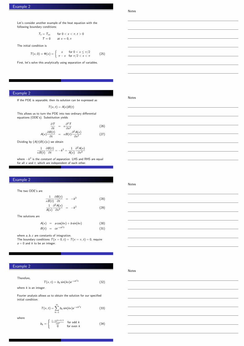
Example 2

Let’s consider another example of the heat equation with thefollowing boundary conditions:

Tt = Txx for 0 < x < π, t > 0

T = 0 at x = 0, π

The initial condition is

T (x , 0) = Φ(x) =

{x for 0 < x ≤ π/2

π − x for π/2 < x < π(25)

First, let’s solve this analytically using separation of variables.

Example 2

If the PDE is separable, then its solution can be expressed as

T (x , t) = A(x)B(t)

This allows us to turn the PDE into two ordinary differentialequations (ODE’s). Substitution yields

∂T

∂t= κ

∂2T

∂x2(26)

A(x)∂B(t)

∂t= κB(t)

∂2A(x)

∂x2(27)

Dividing by (A(t)B(x)κ) we obtain

1

κB(t)

∂B(t)

∂t= −k2 =

1

A(x)

∂2A(x)

∂x2

where −k2 is the constant of separation. LHS and RHS are equalfor all x and t, which are independent of each other.

Example 2

The two ODE’s are

1

κB(t)

∂B(t)

∂t= −k2 (28)

1

A(x)

∂2A(x)

∂x2= −k2 (29)

The solutions are

A(x) = a cos(kx) + b sin(kx) (30)

B(t) = ce−κk2t (31)

where a, b, c are constants of integration.The boundary conditions T (x = 0, t) = T (x = π, t) = 0, requirea = 0 and k to be an integer.

Example 2

Therefore,T (x , t) = bk sin(kx)e−κk

2t (32)

where k is an integer.

Fourier analysis allows us to obtain the solution for our specifiedinitial condition:

T (x , t) =∞∑k=1

bk sin(kx)e−κk2t (33)

where

bk =

{(−1)(k+1)/2

πk2 for odd k0 for even k

(34)

Notes

Notes

Notes

Notes

Example 2

This plot shows the initial temperature distribution Φ(x) andT (x , t) for t = 3π2/80.

As t →∞, T → 0 everywhere.

Numerically solving example 2

Now solve numerically using our difference scheme

T n+1j = (1− 2s)T n

j + s(T nj+1 + T n

j−1) (35)

with s = κ∆t(∆x)2 = 5/11 = 0.45 and ∆x = π/20, where we have

discretized space with J + 1 = 21 points.The discrete boundary and initial conditions are

un0 = un

J = 0 and u0j = Φ(j∆x)

where j = 0, 1, 2, . . . J.


Agrees very well with analytical solution.


However, if we choose s = 5/9 = 0.55, the finite difference schemeyields wild oscillations similar to what we obtained for the impulseIC earlier.

Notes

Notes

Notes

Notes

Stability of finite difference scheme

In the following we will derive the stability criterion for thisdifference scheme:Let’s solve the difference scheme by separation of variables:

T nj = AjBn (36)

Substitution in the difference scheme (eq. (35)) yields

AjBn+1 = (1− 2s)AjBn + s(Aj+1Bn + Aj−1Bn) (37)

Dividing by AjBn we get

Bn+1

Bn= ξ = 1− 2s + s

Aj+1 + Aj−1

Aj(38)

where ξ is the constant of separation.


Thus,Bn+1

Bn= ξ (39)

which has the solutionBn = ξnB0 (40)

where B0 is some constant.Now solve the spatial part:

1− 2s + sAj+1 + Aj−1

Aj= ξ (41)

We wish to investigate the eigenmodes of the solution. Therefore,assume a plane wave solution with wave number k (ignoreboundary conditions for this analysis):

Aj = e ikj∆x (42)


Substituting yields

1− 2s + se ik(j+1)∆x + e ik(j−1)∆x

e ikj∆x= ξ

1− 2s + s(e ik∆x + e−ik∆x) = ξ

1− 2s + 2s cos(k∆x) = ξ

1− 2s(1− cos(k∆x)) = ξ

1− 4s

(sin

(k∆x

2

))2

= ξ

For the difference scheme to be stable, require

|ξ(k)| ≤ 1 for all k (43)

since the amplitude grows as ∝ ξn (eq. (40))


Therefore, ∣∣∣∣∣1− 4s

(sin

(k∆x

2

))2∣∣∣∣∣ ≤ 1

for all k . This leads to the following stability criterion:

4s ≤ 22κ∆t

(∆x)2≤ 1

Physically, this means that the maximum allowed time step ∆t isthe diffusion time across a cell of size ∆x (up to a numerical

factor). The diffusion time across some length λ goes as tλ ∼ λ2

κ

Notes

Notes

Notes

Notes

von Neumann stability analysis

This is the von Neumann stability analysis:

The von Neumann analysis looks at the evolution of theeigenmodes of the solution by substituting

unj = ξne ikj∆x

into the difference equation, where ξ(k) is the amplificationfactor

For the difference scheme to be stable, require

|ξ(k)| ≤ 1 + O(∆t) for all k

Otherwise, eigenmodes grow exponentially in time.

Notes

Notes

Notes

Notes

example: heat ow solving heat ow with an integral … heat ow let us rst solve the heat equation...

Documents