a numerical study for the homogenization of one

Int. J. of Computing Science and Mathematics, Vol. x, No. x, xxxx 1

A Numerical Study for the Homogenization

of One-Dimensional Models describing the

Motion of Dislocations

A. Ghorbel1,∗, P. Hoch2 and R. Monneau1

1 CERMICS, Ecole Nationale des Ponts et Chaussees,6 & 8, avenue Blaise Pascal, cite Descartes,Champs-sur-Marne, 77455 Marne-la-Vallee Cedex 2, FranceE-mail: [email protected], [email protected] CEA/DAM Ile de France, Service DCSA/SSEL, BP 12, 91680Bruyeres Le Chatel.E-mail: [email protected]∗Corresponding author

Abstract: In this paper we are interested in the collective motionof dislocations defects in crystals. Mathematically we study the ho-mogenization of a non-local Hamilton-Jacobi equation. We prove somequalitative properties on the effective hamiltonian. We also provide anumerical scheme which is proved to be monotone under some suitableCFL conditions. Using this scheme, we compute numerically the effec-tive hamiltonian. Furthermore we also provide numerical computationsof the effective hamiltonian for several models corresponding to the dy-namics of dislocations where no theoretical analysis is available.

Keywords: continuous viscosity solution, Dislocations dynamics, eikonalequation, effective hamiltonian, finite difference scheme, Hamilton-Jacobiequation, non-local equation, numerical homogenization, Peach-Koehlerforce, transport equation.

Reference

Biographical Notes: Amin Ghorbel is a PhD student in the last

year in CERMICS at the Ecole Nationale des Ponts et Chaussees. Hisadvisor is Regis Monneau, Professor in CERMICS.

Philippe Hoch works as a researcher ingineer in the CEA(Commissariata l’Energie Atomique).

1 Introduction

In this paper we study the homogenization of non-local Hamilton-Jacobi equa-tions modelling dislocations dynamics, we propose a scheme and provide numericalsimulations for several models.

Copyright c© 200x Inderscience Enterprises Ltd.

2 A. Ghorbel, P. Hoch and R. Monneau

1.1 Physical modelling of dislocations dynamics

In this work, we are interested in the collective behaviour of several dislocationsmoving in a crystal. Dislocations are defects present in real crystals and are at theorigin of the plastic behaviour of metals. We refer to Hirth and Lothe (1992) for aphysical description of dislocations.In our work and in the simplest case, we consider a particular geometry of paralleldislocations lines moving in the same plane. This particular geometry can be mod-eled by a 1D problem where the position of the dislocations is given by the pointx ∈ R where a function u(x, t) takes integer values. In the simplest case, we assumethat u satisfies the following non-local Hamilton-Jacobi equation (see Ghorbel andMonneau (2006) and Imbert et al. (2006) for a study of a similar model)

∂u

∂t(x, t) = c[u](x, t)

∣

∣

∣

∣

∂u

∂x(x, t)

∣

∣

∣

∣

in R× (0, +∞)

c[u](x, t) = A + c1(x) + cint[u](x, t)

cint[u](x, t) =

∫

R

c0(x′) u(x− x′, t) dx′

(1)

with initial condition

u(x, 0) = u0(x) on R (2)

Here c[u] denotes the velocity of the dislocations. It is the sum of three terms: cint

is the contribution created by the interactions with all the dislocations, and is givenby a convolution, c1 is a microscopic field created by the other defects in the crystaland A ∈ R is the exterior applied stress.

We will study problem (1) and similar equations in the framework of viscositysolutions. Let us recall that the notion of viscosity solution was first introducedby Crandall and Lions (1981) for first order Hamilton-Jacobi equations. For anintroduction to this notion, see in particular the books of Barles (1994), and ofBardi and Capuzzo-Dolcetta (1997), and the User’s guide of Crandall, Ishii andLions (1992).

We assume that the kernel c0 satisfies

c0(x) = c0(−x) and

∫

R

c0(x) dx = 0 . (3)

We also assume the periodicity and the regularity of the micro-stress c1

c1(x + 1) = c1(x) on R , and c1 is Lipschitz-continuous (4)

1.2 Goal of the paper

We want to understand the properties of the solutions of (1) for A = 0 at alarge scale defining

uε(x, t) = ε u

(

x

ε,t

ε

)

A Numerical Homogenization of Models describing the Motion of Dislocations 3

where ε is the ratio between the mesoscopic scale and the microscopic scale associ-ated to dislocations (like distances between obstacles to the motion of dislocations).

Homogenization of Hamilton-Jacobi Equations was studied by Lions, Papanicolaouand Varadhan (1986) and this work was followed by a large literature on the subject,that would be difficult to cite here.

For this equation (see Imbert et al. (2006)) and for a certain class of kernels c0, itis known that uε converges to u0, solution of

∂u0

∂t= H

(

I1u0,

∂u0

∂x

)

where I1 is a non-local Levy operator, and H is the effective hamiltonian given bythe following definition.

Definition 1.1. (Effective hamiltonian)We assume (4). For (A, p) ∈ R×R, the effective hamiltonian H(A, p) is defined by

H(A, p) = limt→+∞

w(x, t)

t(independent on x) (5)

where w solves the ”cell problem”, i.e. w solves (1) with w(x, 0) = px .

Then the goal of the present paper is to compute numerically H(A, p) for equation(1) for specific kernels c0. In particular, we numerically check that the ergodicityproperty (5) holds for general kernels c0 (like for instance for the Peierls-Nabarromodel, see subsection 5.2), even in the case where the equation has no compari-son principle and it is even not clear if (5) holds theoretically. We also do somesimulations for some similar equations or systems of equations. To this end, weimplemented several numerical schemes.

1.3 Brief presentation of our results

We present here properties of the effective hamiltonian and the scheme used tocompute it numerically. We prove the following qualitative result on the effectivehamiltonian.

Theorem 1.2. (Monotonicity of the effective hamiltonian)For the choice c0 = −δ0 + J with δ0 is a Dirac mass and J ∈ C∞(R) is such that

J(−x) = J(x) ≥ 0 ;

∫

R

J(x) dx = 1 and

∫

R

|x| J(x) dx < +∞

c2 := infδ∈[0,1)

∫

R

min (J(z), J(z + δ)) dz > 0

(6)

Then the effective hamiltonian given in Definition 1.1 satisfies

1. H(A, p) is non-decreasing in A.


2. If

∫

R

c1(x) dx = 0 then H(0, p) = 0 and AH(A, p) is non-decreasing in |p|and satisfies

sgn(A)

(

|A|+ 1 +2

c2

)

≥ sgn(A)∂H

∂|p| (A, p) ≥ 0 .

We build a finite difference scheme of order one in space and time using an explicitEuler scheme in time and an upwind scheme in space. Given a mesh size ∆x, ∆tand a lattice Id = {(i∆x, n∆t); i ∈ Z, n ∈ N}, (xi, tn) denotes the node (i∆x, n∆t)and vn = (vn

i )i the values of the numerical approximation of the continuous solutionu(xi, tn). We then consider the following numerical scheme:

v0i = u0(xi), vn+1

i = vni + ∆t ci(v

n)×{

D+x vn

i if ci(vn) ≥ 0

D−

x vni if ci(v

n) < 0(7)

with D−

x vni =

vni − vn

i−1

∆xand D+

x vni =

vni+1 − vn

i

∆x. The discrete velocity is

ci(vn) = A + c1(xi) + cint

i (vn) (8)

We approximate the non-local term c0 ? u by

cinti (vn) = −vn

i +∑

l∈Z

Jl vni−l ∆x

Ji =1

∆x

∫

Ii

J(x) dx and Ii =

[

xi −∆x

2, xi +

∆x

2

]

.

(9)

Several works have been done for the discretization of more general first orderHamilton-Jacobi equations (even with boundary conditions). We refer in particularto the work of Abgrall (2003).Then we have the following result about monotonicity of the scheme (7) for thespecial kernel c0 = −δ0 + J .

Theorem 1.3. (Monotonicity of the scheme)We assume that

v0i+1 ≥ v0

i , ∀ i ∈ Z(10)

(respectively w0i+1 ≥ w0

i , ∀ i ∈ Z)(11)

If the time step ∆t satisfies

∆t ≤(

supj∈Z

|cj+1(vk)− cj(vk)|∆x

)−1

, for 0 ≤ k ≤ n(12)

(respectively ∆t ≤(

supj∈Z

|cj+1(wk)− cj(wk)|∆x

)−1

, for 0 ≤ k ≤ n)(13)

Then we have the monotonicity preservation:

vki+1 ≥ vk

i , ∀ i ∈ Z , ∀ 0 ≤ k ≤ n + 1(14)

(respectively wki+1 ≥ wk

i , ∀ i ∈ Z , ∀ 0 ≤ k ≤ n + 1(15)


Assume moreover that

v0i ≥ w0

i , ∀ i ∈ Z .(16)

If the time step ∆t satisfies moreover

∆t supj∈Z

{

max

(

vkj+1 − vk

j

∆x,wk

j+1 − wkj

∆x

)}

≤ 1

2for 0 ≤ k ≤ n(17)

and

∆t

∆x≤ 1

2

(

supj∈Z

{

max(∣

∣cj(vk)∣

∣ ,∣

∣cj(wk)∣

∣

)}

)−1

for 0 ≤ k ≤ n(18)

Then

vki ≥ wk

i , ∀ i ∈ Z for 0 ≤ k ≤ n + 1 .(19)

Remark 1.4. There would be no monotonicity of the scheme if J would be negative.

We use this scheme to compute numerically an approximation Hnum(A, p) of H(A, p).We numerically check that Hnum(A, p) satisfies the monotonicity properties givenin Theorem 1.2. We also compute the effective hamiltonian for other similar equa-tions (like for instance the case with Peierls-Nabarro kernel, see subsection 5.2),and for some systems of equations (see Section 6).

There are very few works on numerics for homogenization. Up to our knowledge,let us mention for convex first order hamiltonians the work of Gomes and Oberman(2004) computing the effective hamiltonian using a variational approach and thework of Rorro (2006) using semi-Lagrangian schemes.

1.4 Organization of the paper

In Section 2, we give the proof of Theorem 1.2. In Section 3, we study the nu-merical scheme and prove Theorem 1.3. In Section 4, we give numerical simulationscorresponding to the scheme of Theorem 1.3. In Section 5, we present numericalsimulations for similar equations with for instance the Peierls-Nabarro kernel. InSection 6, we present numerical simulations for systems of equations for two typesof dislocations. Finally in the Appendix we provide the proof of a technical Lemma(Lemma 2.1) and give a brief derivation of the kernel for walls of dislocations.

2 Qualitative properties of the effective hamiltonian

Before to prove Theorem 1.2, we need the following lemma with the proof givenin the Appendix.

Lemma 2.1. (Coercivity of the convolution)Assume J satisfies (6) and c0 = −δ0 + J . If u ∈ C0

b (R) is maximal at Y ∈ R andminimal at y ∈ R and |Y − y| < 1 then

(

c0 ? u)

(Y )−(

c0 ? u)

(y) ≤ −c2 (u(Y )− u(y))


To keep light notation, we denote in this section by M the operator such that

(Mv)(x) =(

c0 ? v)

(x) = −v(x) +

∫

R

J(z)v(x− z) dz.(20)

We will also need the following result.

Lemma 2.2. (Existence of sub and supercorrectors)For any p ∈ R and A ∈ R, there exist λ ∈ R, a subcorrector v(x) and a supercor-rector v(x) which are 1-periodic in x and satisfy

λ ≤ |p + ∂xv|(

c1 + A + Mv)

, with p(p + ∂xv) ≥ 0 on R

λ ≥ |p + ∂xv|(

c1 + A + Mv)

, with p(p + ∂xv) ≥ 0 on R

with

max v −min v ≤ 2

c2

∣

∣c1∣

∣

L∞(R)and max v −min v ≤ 2

c2

∣

∣c1∣

∣

L∞(R)

where c2 given in (6).

The proof of Lemma 2.2 is a slight adaptation of the work of Imbert et al. (2006).We give below a quick proof of this fact.

Skech of the proof of Lemma 2.2

Let us work in the case p > 0 (the case p < 0 is similar, and for the case p = 0, wehave λ = 0 with a corrector equal to zero).Step 1Using the theory developed in Imbert et al. (2006), let us start to consider (using

the fact that

∫

R

|x| J(x) dx < +∞), for p > 0, the solution u of

{

ut = |∂xu|(c1 + A + M(u− p ·))u(x, t = 0) = px

then ω(t) = infx

∂xu(t, x) formally satisfies

ωt ≥ |ω|(∂xc1 + Mω) ≥ |ω|(∂xc1) with ω(0) = p > 0

and therefore the bound from below on the possible exponential decay of ω impliesthat

∂xu ≥ 0

This result can be justified rigorously using some classical viscosity arguments (asin Imbert et al. (2006)). We also know that u(t, x) − px is 1-periodic in x. Wealready know by Imbert et al. (2006) that there exists a unique λ ∈ R such thatv(t, x) = u(t, x)− px−λt is bounded. Moreover λ = H(A, p). Let us now define Yt

and yt such that M(t) := maxx

v(t, x) = v(t, Yt) and m(t) := minx

v(t, x) = v(t, yt)

and |Yt − yt| < 1, we get formally

λ + M ′(t) ≤ |p|(

c1(Yt) + A + (Mv)(Yt))


λ + m′(t) ≥ |p|(

c1(yt) + A + (Mv)(yt))

which implies for p 6= 0 that ω(t) = M(t)−m(t) satisfies

ω′(t)/|p| − ((Mv)(Yt)− (Mv)(yt)) ≤ c1(Yt)− c1(yt)

And then by Lemma 2.1, we get that

ω′(t)/|p|+ c2ω(t) ≤ c1(Yt)− c1(yt) with ω(0) = 0 .

This inequality can be justified rigorously by routine viscosity arguments. Wededuce that for every t ≥ 0

ω(t) = maxx

v(t, x)−minx

v(t, x) ≤ 2

c2|c1|L∞(R)

Step 2Considering the semi-relaxed limits of u(t, x)− px− λt with the suppremum (resp.the infimum) in time, we build a subsolution v (resp. a supersolution v) of thefollowing equation

λ = |p + ∂xv|(

c1 + A + Mv)

which satisfies the expected properties.

This ends the proof of the Lemma.

2

Proof of Theorem 1.2

1) We first prove the monotonicity of H(A, p) in A. Let us consider A2 > A1,λi = H(Ai, p), i = 1, 2 and a subcorrector v1 for (A, p) then we have

λ1 ≤ |p + ∂xv1|(

c1 + A1 + Mv1

)

≤ |p + ∂xv1|(

c1 + A2 + Mv1

)

This shows v1(x)+px+λ1t is a subsolution to the cell problem which impliesthat λ2 ≥ λ1 i.e. H(A2, p) ≥ H(A1, p).

2) We now prove that H(0, p) = 0 in the case

∫

(0,1)

c1 = 0 . Let us define v0 as

the periodic solution of

Mv0 = −c1 on R (21)

such that

∫

(0,1)

v0 = 0. We see that v0 is a corrector for the cell problem with

λ = 0 = H(0, p).


3) Let us now show the monotonicity in |p| in the case

∫

(0,1)

c1 = 0. For p2 > p1 > 0

and A > 0 such that λ1 > 0 with λi = H(A, pi), i = 1, 2 (the other cases aresimilar), let us consider a subcorrector v1 satisfying

0 < λ1 ≤ (p1 + ∂xv1)(

c1 + A + Mv1

)

with p1 + ∂xv1 ≥ 0

and a supercorrector v1 satisfying

λ1 ≥ (p1 + ∂xv1)(

c1 + A + Mv1

)

with p1 + ∂xv1 ≥ 0

From Lemma 2.2, we also know that we can bound these sub/supercorrectors

by2

c2|c1|L∞(R). Therefore

0 ≤ c1 + A + Mv1 and

(

1 +2

c2

)

|c1|L∞(R) ≥ c1 + Mv1 .

And then

λ1 ≤ λ1 + (p2 − p1)(

c1 + A + Mv1

)

≤ (p2 + ∂xv1)(

c1 + A + Mv1

)

which implies λ2 ≥ λ1 > 0 .

Similarly, we have

λ1 +

((

1 +2

c2

)

|c1|L∞(R) + A

)

(p2 − p1)≥ λ1 + (p2 − p1)(

c1 + A + Mv1

)

≥ (p2 + ∂xv1)(

c1 + A + Mv1

)

which implies λ2 ≤ λ1 +

((

1 +2

c2

)

|c1|L∞(R) + A

)

(p2 − p1) and gives the

result.

2

3 Monotonicity of the scheme

In this section we prove Theorem 1.3 . We will use the following result (conse-quence of Lemma 2.5.2 in Ghorbel and Monneau (2006))

Lemma 3.1. (A monotonicity preserving scheme for prescribed velocity)We assume that

vn+1i = vn

i +∆t

∆xcni ×

{

vni+1 − vn

i if cni ≥ 0

vni − vn

i−1 if cni < 0

and

∆t ≤ 1

2

(

supj∈Z

∣

∣ckj+1 − ck

j

∣

∣

∆x

)−1

for 0 ≤ k ≤ n(22)


Ifv0

i+1 ≥ v0i , ∀ i ∈ Z

thenvk

i+1 ≥ vki , ∀ i ∈ Z , for 0 ≤ k ≤ n + 1 .

Proof of Theorem 1.3

Let (vni )i∈Z,n∈N and (wn

i )i∈Z,n∈N two discrete solutions, such that v0i and w0

i are non-

decreasing in i ∈ Z. We set Mn(v) := supi∈Z

vni+1 − vn

i

∆xand Mn(w) := sup

i∈Z

wni+1 − wn

i

∆x.

One write the numerical scheme for v (and the same for w)

vn+1i = vn

i +∆t

∆xci(v

n)×{

vni+1 − vn

i if ci(vn) ≥ 0

vni − vn

i−1 if ci(vn) < 0

(23)

with ci(vn) defined in (8)-(9). Let us assume that vk

i ≥ wki , ∀ i ∈ Z, ∀ 0 ≤ k ≤ n.

Let us prove that it is still true for k = n + 1.

Case 1: We assume that ci(vn) ≥ 0 and ci(w

n) ≥ 0 .We have

vn+1i − wn+1

i = vni − wn

i +∆t

∆x

(

ci(vn)(

vni+1 − vn

i

)

− ci(wn)(

wni+1 − wn

i

))

.

One can add and substract∆t

∆xci(w

n)(

vni+1 − vn

i

)

, and one obtains

vn+1i − wn+1

i = (vni − wn

i )

(

1− ∆t

∆xci(w

n)

)

+∆t

∆xci(w

n)(

vni+1 − wn

i+1

)

+∆t

∆x(ci(v

n)− ci(wn))(

vni+1 − vn

i

)

≥ (vni − wn

i )

(

1− ∆t

∆xci(w

n)

)

+∆t

∆x(ci(v

n)− ci(wn))(

vni+1 − vn

i

)

where we have used the fact that vni+1 ≥ wn

i+1. Since

ci(vn) = A + c1(xi)− vn

i +∑

j∈Z

Jjvni−j ∆x(24)

the difference between the discrete velocities can be written as

ci(vn)− ci(w

n) = − (vni − wn

i ) +∑

j∈Z

Jj

(

vni−j − wn

i−j

)

∆x(25)

and then we get (using Jj ≥ 0 and vni−j − wn

i−j ≥ 0)

vn+1i − wn+1

i ≥ (vni − wn

i )

(

1− ∆t

∆xci(w

n)

)

− ∆t

∆x(vn

i − wni ) (vn

i+1 − vni )

≥ (vni − wn

i )

(

1− ∆t

∆xci(w

n)−Mn(u)∆t

) (26)


Therefore we have

vn+1i − wn+1

i ≥ (vni − wn

i )

(

1− ∆t

∆xci(w

n)−Mn(u)∆t

)

. (27)

It is then sufficient to have the following two restrictions on the time step

∆t

∆x≤(

2 supj∈Z

|cj(vn)|)−1

and Mn(u)∆t ≤ 1

2

to deduce that the scheme is monotone in this case.

Case 2: We assume that ci(vn) ≤ 0 and ci(w

n) ≤ 0 .We compute

vn+1i − wn+1

i = vni − wn

i +∆t

∆xci(v

n)(vni − vn

i−1)− ∆t

∆xci(w

n)(wni − wn

i−1).

One can add and substract∆t

∆xci(v

n)(

wni − wn

i−1

)

, one obtains

vn+1i − wn+1

i = (vni − wn

i )

(

1 +∆t

∆xci(v

n)

)

+∆t

∆x(ci(v

n)− ci(wn)) (wn

i − wni−1)

−∆t

∆xci(v

n)(vni−1 − wn

i−1)

Since ci(vn) < 0 and vn

i−1 ≥ wni−1, we get

vn+1i − wn+1

i ≥ (vni − wn

i )

(

1 +∆t

∆xci(v

n)

)

+∆t

∆x(ci(v

n)− ci(wn)) (wn

i − wni−1)

≥ (vni − wn

i )

(

1 +∆t

∆xci(v

n)−Mn(w)∆t

)

≥ 0

if∆t

∆x≤(

2 supj∈Z

|cj(un)|)−1

and Mn(v)∆t ≤ 1

2.

Case 3: We assume that ci(vn) ≥ 0 and ci(w

n) < 0 .We compute

vn+1i − wn+1

i = vni − wn

i +∆t

∆xci(v

n)(vni+1 − vn

i )− ∆t

∆xci(w

n)(wni − wn

i−1)

≥ vni − wn

i

because vni+1− vn

i ≥ 0 and wni −wn

i−1 ≥ 0. It is then sufficient to assume that

∆t ≤(

supj∈Z

|cj+1(vk)− cj(vk)|∆x

)−1

for 0 ≤ k ≤ n(28)

and ∆t ≤(

supj∈Z

|cj+1(wk)− cj(wk)|∆x

)−1

for 0 ≤ k ≤ n(29)

to guarantee the monotonicity of v and the monotonicity of w using Lemma3.1.


Case 4: We assume that ci(vn) < 0 and ci(w

n) ≥ 0 .We compute

vn+1i − wn+1

i = vni − wn

i +∆t

∆xci(v

n)(vni − vn

i−1)− ∆t

∆xci(w

n)(wni − wn

i−1).

But0 > ci(v

n)− ci(wn)

= −(vni − wn

i ) +∑

l

Jl(vni−l − wn

i−l)

≥ −(vni − wn

i )

and for general c+ ≥ 0, c− ≤ 0 and a, b ≥ 0 we have

|c−a− c+b| ≤ max(a, b) |c+ − c−|

and then∣

∣ci(vn)(vn

i − vni−1)− ci(w

n)(wni+1 − wn

i+1)∣

∣≤ ∆x max(Mn(v),Mn(w)) |ci(vn)− ci(w

n)|≤ ∆x max(Mn(v),Mn(w))(vn

i − wni )

Therefore

vn+1i − wn

i ≥ (vni − wn

i )(1−∆t max(Mn(v),Mn(w)))

≥ 0

if we assume ∆t max(Mn(v),Mn(w)) ≤ 1 and (28)-(29).

2

4 Computation of the effective hamiltonian for equation (1)

We recall here that the effective hamiltonian is given in Definition 1.1. Numer-ically we compute H(A, p) for

p =P

Qfor a fixed Q ∈ N \ {0} and P ∈ Z (30)

Because p is given by (30), we know that the solution w to (1) with initial valuegiven by w(x, 0) = px satisfies

w(x + Q, t) = w(x, t) + P .

For this reason, numerically we restrict the computation on the interval

[

−Q

2,Q

2

]

with periodic boundary conditions for w(x, t) = w(x, t) − px and we write the

equation for w. In particular we also choose ∆x such thatQ

∆x∈ N \ {0}.

We then use the numerical scheme of Theorem 1.3 with ∆t satisfying the CFLconditions stated in Theorem 1.3, which guarantees the monotonicity of the scheme.


4.1 The method to compute the effective hamiltonian

Here we describe two possible strategies to compute numerically the effectivehamiltonian Hnum(A, p).

Method 1: Using the numerical solution wn of (7), we take its values at twodiscrete times t1 > 0 and t2 > 0 at a discrete point xref and we define

Hnum(A, p) =v(xref , t2)− v(xref , t1)

t2 − t1for t2−t1 large enough, which is difficult

to fix in practice.

Method 2: We follow the position of a dislocation (as a marker) starting froma point xref at time t1 and waiting until it passes a second time (in the”periodic” interval [−Q/2, Q/2]) at the same point at time t2, and we define

Hnum(A, p) =|P |

t2 − t1with p =

P

Q(see Figure 1). Here

Hnum(A, p)

pcan be

interpreted as an effective velocity.

In practice we prefer to use the Method 2 in general, because, given a timet1 large enough, it provides naturally a time t2. On the contrary, the resultgiven by the Method 1 can be more sensitive to the choice of t2 with respectto t1.

xref

t

t2

t1x

t′2

−Q

2

Q

2

Figure 1 Tracking the trajectory of a dislocation until it comes back to the initialposition

4.2 Results of the numerical simulations

Let us recall that the convolution is written as

c0 ?R

w = c0 ?R

(w − px)

= −w + J ?R

w

= −w + J∗ ?[−Q

2 ,Q

2 )w

(31)

with

J∗(x) =∑

k∈Z

J(x + kQ) . (32)


For the present simulations we choose

J∗(x) =1

Qfor x ∈

[

−Q

2,Q

2

)

. (33)

We choose

c1(x) = B sin(2πkx) with k ∈ N \ {0}. (34)

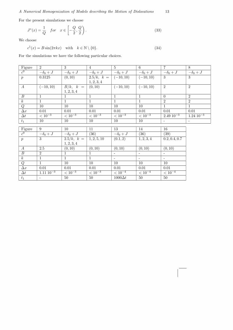
For the simulations we have the following particular choices.

Figure 2 3 4 5 6 7 8c0 −δ0 + J −δ0 + J −δ0 + J −δ0 + J −δ0 + J −δ0 + J −δ0 + J

p 0.3125 (0, 10) 2.5/k, k =1, 2, 3, 4

(−10, 10) (−10, 10) 3 3

A (−10, 10) B/k, k =1, 2, 3, 4

(0, 10) (−10, 10) (−10, 10) 2 2

B 1 1 1 1 1 0 2

k 1 1 1 1 1 2 2

Q 10 10 10 10 10 1 1∆x 0.01 0.01 0.01 0.01 0.01 0.01 0.01

∆t < 10−3 < 10−3 < 10−3 < 10−3 < 10−3 2.49 10−3 1.24 10−3

t1 10 10 10 10 10 - -

Figure 9 10 11 13 14 16

c0 −δ0 + J −δ0 + J (36) −δ0 + J (36) (39)

p 3 2.5/k, k =1, 2, 3, 4

1, 2, 5, 10 (0.1, 2) 1, 2, 3, 4 0.2, 0.4, 0.7

A 2.5 (0, 10) (0, 10) (0, 10) (0, 10) (0, 10)

B 2 1 1 - - -k 1 1 1 - - -

Q 1 10 10 10 10 10

∆x 0.01 0.01 0.01 0.01 0.01 0.01∆t 1.11 10−3 < 10−3 < 10−3 < 10−4 < 10−4 < 10−4

t1 - 50 50 1000∆t 50 50


-3

-2

-1

0

1

2

3

-10 -5 0 5 10

Effe

ctiv

e H

amilt

onia

n

A

Figure 2 Hnum(A, p) for p = 0.3125 and a monotone kernel c0 = −δ0 + J

In Figure 2, we present the numerical effective hamiltonian Hnum(A, p) which ismonotone in A as expected from the first property of Theorem 1.2. Moreover thisreveals the existence of a threshold effect, i.e. the effective hamiltonian is zero ona whole interval of the parameter A. In addition Hnum(A, p) is antisymmetric inA because of the symmetries of c1. For |A| � B = 1, the effective hamiltonian islinear and can be approximated here by Ap which is the classical Orowan law (seeKratochvil et al. (2003)). In addition, we note that Hnum(A, p) behaves like thesquare-root function of A in a neighborhood of the zero-plateau of Hnum.

-1

0

1

2

3

4

5

6

7

8

0 1 2 3 4 5 6 7 8 9 10

Effe

ctiv

e H

amilt

onia

n

p

A=B

A=B/2 A=B/4 A=B/8

Figure 3 Hnum(A, p) as a function of the density p for a monotone kernel c0 = −δ0+J

In Figure 3, the effective hamiltonian Hnum(A, p) is represented as a function of pfor some values of A. We note here the monotonicity of Hnum with respect to p.For a large density of dislocations, the effective hamiltonian Hnum is linear and canagain be approximated by Ap.


0

5

10

15

20

25

0 2 4 6 8 10

Effe

ctiv

e H

amilt

onia

n

A

p=2.5

p=1.25

p=0.625 p=0.3125

Figure 4 Hnum(A, p) as a function of A and a monotone kernel c0 = −δ0 + J

In Figure 4, we present the effective hamiltonian Hnum(A, p) as a function of Afor several densities of dislocations p. Again we check numerically the qualitativeproperties of the effective hamiltonian.


−50

−1

−0.05

−0.001

−5e−05

−1e−06

−5e−08

5e−08

1e−06

5e−05

0.001

0.05

1

50

XY

Z

Effec

tive H

amilt

onian

−77.88

0

77.88

A−10

0

10

p−10

0

10

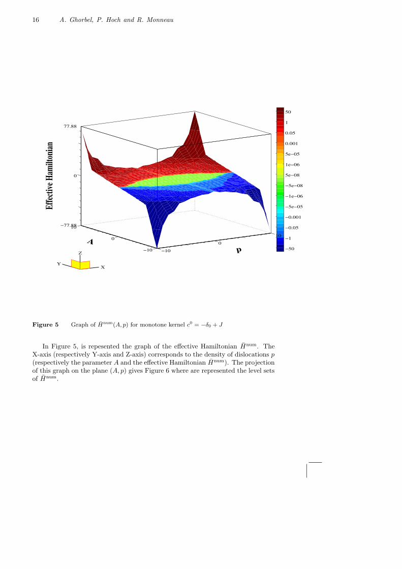
Figure 5 Graph of Hnum(A, p) for monotone kernel c0 = −δ0 + J

In Figure 5, is repesented the graph of the effective Hamiltonian Hnum. TheX-axis (respectively Y-axis and Z-axis) corresponds to the density of dislocations p(respectively the parameter A and the effective Hamiltonian Hnum). The projectionof this graph on the plane (A, p) gives Figure 6 where are represented the level setsof Hnum.


−10 0 10−10

0

10

Effective Hamiltonian

p

A

−50

−1

−0.05

−0.001

−5e−05

−1e−06

−5e−08

5e−08

1e−06

5e−05

0.001

0.05

1

50

−10 0 10−10

0

10

Figure 6 Level sets of the effective hamiltonian Hnum(A, p)

In Figure 6, the central region is the set where there is a pinning of the dislocationson the defects represented by the field c1, i.e. where the effective hamiltonianvanishes. Moreover the monotonicity of Hnum in p reveals that in this model, theability of the dislocations to pass the obstacles, is increased when we increase thedensity of dislocations. This is typically a collective behaviour.

5 Computation of the effective hamiltonian for other equations

In this section we study numerically the effective hamiltonian for models wherein equation (1) the non-local velocity cint[u] is replaced by

cint[u] = c0 ? buc (35)

where b·c is the floor function.Here the positions of dislocations are given by the jumps of buc (see Ghorbel andMonneau (2006)). Let us mention that even for monotone kernel c0, the theoreticalexistence of an effective hamiltonian is not known, we numerically check that this


effective hamiltonian exists in two cases: the monotone kernel (Subsection 5.1) andthe Peierls-Nabarro kernel (Subsection 5.2).

5.1 The monotone kernel with one type of dislocations

In this subsection we set c0 = −δ0 +J with J∗ =1

Qwith the notation of Section

4. This case is strongly related to the homogenization of a Slepcev formulation (seeForcadel et al.).

0

0.5

1

1.5

2

2.5

3

3.5

4

4.5

5

-0.4 -0.2 0 0.2 0.4

t

x

Figure 7 Linear trajectories

0

0.5

1

1.5

2

2.5

3

3.5

4

4.5

5

-0.4 -0.2 0 0.2 0.4

t

x

Figure 8 Pinning of dislocations

First, we represent in Figure 7 the trajectories of 3 dislocations (initially located atx = −1/3, x = 0, x = 1/3) in the case where there are no obstacles (i.e. c1 = 0).In this case the trajectories of dislocations are straight lines. A different situationhappens (see Figure 8), when we add sufficient obstacles in order to obtain thepinning of dislocations (with B ≥ A). This case corresponds to the situation whereHnum is equal to zero.


0

0.5

1

1.5

2

2.5

3

3.5

4

4.5

5

-0.4 -0.2 0 0.2 0.4

t

x

Figure 9 The motion of the dislocations becomes periodic in time

Now, if we increase the parameter A, without changing the obstacles, i.e. with thesame c1, we observe a persistent motion of dislocations (see Figure 9). Numerically,this motion becomes periodic in time. Moreover, we also present in Figure 10 theeffective hamiltonian whose behaviour is similar to the case of Section 4.

0

5

10

15

20

25

0 2 4 6 8 10

Effe

ctiv

e H

amilt

onia

n

A

p=2.5

p=1.25

p=0.625 p=0.3125

Figure 10 Effective hamiltonian Hnum(A, p) as a function of A for c0 ? buc, c0 =−δ0 + J

5.2 The Peierls-Nabarro kernel with one type of edge dislocations

In this subsection, we consider the Peierls-Nabarro kernel (see Hirth and Lothe(1992); Alvarez et al. (2006)) given by

c0(x) =−µ∣

∣

∣

~b∣

∣

∣

2

2π(1− ν)

x2 − ζ2

(x2 + ζ2)2. (36)


where ν =λ

2(λ + µ)is the Poisson ratio and λ and µ > 0 are the Lame coefficients

for isotropic elasticity and ~b is the Burgers vector. We chooseµ∣

∣

∣

~b∣

∣

∣

2

2π(1− ν)= 1 and

ζ = 0.01 for our simulations.Again we compute the effective hamiltonian in Figure 11 which turns out to providea behaviour similar to the one of Section 4.

0

20

40

60

80

100

0 2 4 6 8 10

Effe

ctiv

e H

amilt

onia

n

A

p=2 p=1

p=10

p=5

Figure 11 Graph of Hnum(A, p) for Peierls-Nabarro model with one type of edgedislocations

6 Computation of the effective hamiltonian for systems of equations

In this section, we consider systems of equations describing the motion of dis-locations of opposite Burgers vector (+~b ) and (−~b ). More precisely we studynumerically the following system

∂u+

∂t(x, t) = −c[u+, u−](x, t)

∣

∣

∣

∣

∂u+

∂x(x, t)

∣

∣

∣

∣

in R× (0, +∞)

∂u−

∂t(x, t) = c[u+, u−](x, t)

∣

∣

∣

∣

∂u−

∂x(x, t)

∣

∣

∣

∣

in R× (0, +∞)

u+(x, 0) = p+x on R

u−(x, 0) = p−x on R

(37)

where

c[u+, u−](x, t) = A + c0 ?(

bu+(·, t)c − bu−(·, t)c)

. (38)

Here the positions of dislocations of Burgers vector (+~b ) (respectively (−~b )) are rep-resented by the jumps of bu+(·, t)c (respectively bu+(·, t)c). The motion is schemat-ically represented on Figure 12.


x

+ + + + + + + + +

− − − − − − − − −

motion of dislocation +

motion of dislocation −

Figure 12 Opposite motion of dislocations + and −

In the following three subsections we will compute the numerical effective hamilto-nian for the two types of dislocations Hnum(A, p) with the same densities p = p+ =

p− (or the velocityHnum(A, p)

p) using a numerical method similar to the one used

in Sections 4 and 5. We present successively our result in the case of monotonekernel, Peierls-Nabarro kernel for edge dislocations, and the kernel describing themotion of walls of dislocations.

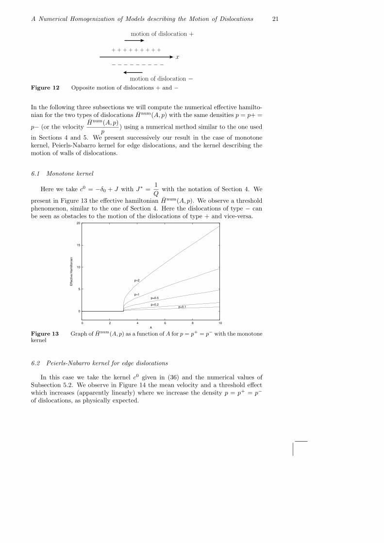
6.1 Monotone kernel

Here we take c0 = −δ0 + J with J∗ =1

Qwith the notation of Section 4. We

present in Figure 13 the effective hamiltonian Hnum(A, p). We observe a thresholdphenomenon, similar to the one of Section 4. Here the dislocations of type − canbe seen as obstacles to the motion of the dislocations of type + and vice-versa.

0

5

10

15

20

0 2 4 6 8 10

Effe

ctiv

e H

amilt

onia

n

A

p=2

p=1p=0.5

p=0.2p=0.1

Figure 13 Graph of Hnum(A, p) as a function of A for p = p+ = p− with the monotonekernel

6.2 Peierls-Nabarro kernel for edge dislocations

In this case we take the kernel c0 given in (36) and the numerical values ofSubsection 5.2. We observe in Figure 14 the mean velocity and a threshold effectwhich increases (apparently linearly) where we increase the density p = p+ = p−

of dislocations, as physically expected.


0

2

4

6

8

10

0 2 4 6 8 10

Effe

ctiv

e V

eloc

ity

A

p=1 p=2 p=3 p=4

Figure 14 Effective velocityHnum(A, p)

pas a function of A for p = p+ = p− in the

case of Peierls-Nabarro kernel

6.3 Kernel for walls of dislocations

Here we take

c0(x) =∂σ

∂x(x) with σ(x) =

µ∣

∣

∣

~b∣

∣

∣

2

π

1− ν

xε

(

cosh(2πx

ε)− 1

) (39)

with µ is a Lame coefficient, ν is the Poisson ratio, ~b is the Burgers vector and εis the distance between dislocations along the y direction (see Figure 15 and theAppendix 7.2).

y

x

ε

+ + +

− − −

− − −

− − −

+ + +

+ + +

+ + +

− − −

+ + +

− − −

motion of wall +

motion of wall −

Figure 15 Walls of dislocations + and walls of dislocations −


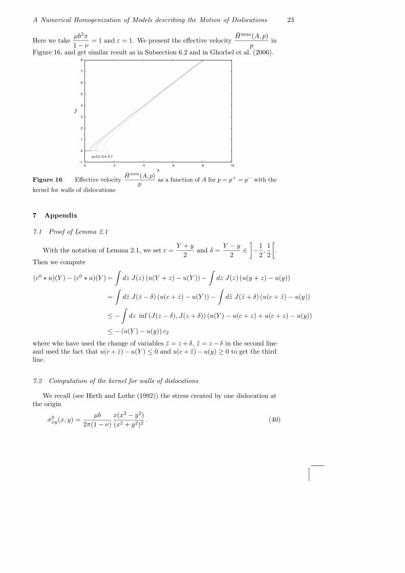
Here we takeµb2π

1− ν= 1 and ε = 1. We present the effective velocity

Hnum(A, p)

pin

Figure 16, and get similar result as in Subsection 6.2 and in Ghorbel et al. (2006).

-1

0

1

2

3

4

5

6

7

8

0 2 4 6 8 10

v eff

A

p=0.2, 0.4, 0.7

Figure 16 Effective velocityHnum(A, p)

pas a function of A for p = p+ = p− with the

kernel for walls of dislocations

7 Appendix

7.1 Proof of Lemma 2.1

With the notation of Lemma 2.1, we set c =Y + y

2and δ =

Y − y

2∈]

−1

2,

1

2

[

.

Then we compute

(c0 ? u)(Y )− (c0 ? u)(Y ) =

∫

dz J(z) (u(Y + z)− u(Y ))−∫

dz J(z) (u(y + z)− u(y))

=

∫

dz J(z − δ) (u(c + z)− u(Y ))−∫

dz J(z + δ) (u(c + z)− u(y))

≤ −∫

dz inf (J(z − δ), J(z + δ)) (u(Y )− u(c + z) + u(c + z)− u(y))

≤ − (u(Y )− u(y)) c2

where whe have used the change of variables z = z + δ, z = z− δ in the second lineand used the fact that u(c + z)− u(Y ) ≤ 0 and u(c + z)− u(y) ≥ 0 to get the thirdline.

7.2 Computation of the kernel for walls of dislocations

We recall (see Hirth and Lothe (1992)) the stress created by one dislocation atthe origin

σ0xy(x, y) =

µb

2π(1− ν)

x(x2 − y2)

(x2 + y2)2. (40)


Now the stress created by a wall of dislocations at the positions x = 0, y = kε fork ∈ Z is given by

σxy(x, y) =∑

k∈Z

σ0xy(x, y − kε)

=µbπ

1− ν

xε

(

cosh(2π xε) cos(2π y

ε)− 1

)

(

cosh(2πx

ε)− cos(2π

y

ε))2 .

(41)

(see Hirth and Lothe (1992) page 733, formula (19-73)). Then

c0(x) = b∂σxy

∂x(x, 0) =

∂σ

∂x(x) (42)

with σ(x) = b σxy(x, 0).

Acknowledgements

The authors would like to thank O. Alvarez, M. El Rhabi, A. Finel and Y.Le Bouar for fruitful discussions. This work was supported by the contract JC1025 called ”ACI jeunes chercheuses et jeunes chercheurs” of the French Ministryof Research (2003-2007).

References

Abgrall, R. (2003) ‘Numerical discretization of boundary conditions for first orderHamilton-Jacobi equations’, SIAM J. Numer. Anal., Vol. 41, No. 6, pp.2233–2261.

Alvarez, O., Hoch, P., Le Bouar, Y. and Monneau, R. (2006) ‘Dislocation dynamics:short time existence and uniqueness of the solution’, Arch. Ration. Mech. Anal.,Vol. 181, No. 3, pp.449–504.

Bardi, M. and Capuzzo-Dolcetta, I. (1997) ‘Optimal Control and Viscosity Solutionsof Hamilton-Jacobi-Bellman Equations’, Birkhauser Boston Inc., Boston.

Barles, G. (1994) ‘Solutions de Viscosite des Equations de Hamilton-Jacobi’,Springer-Verlag, Berlin.

Crandall, M.G. and Lions, P.-L. (1981) ‘Conditions d’unicite pour les solutionsgeneralisees des equations de Hamilton-Jacobi du premier ordre’, C. R. Acad.Sci. Paris Ser. I Math., Vol. 292, pp.183–186.

Crandall, M.G., Ishii, H. and Lions, P.-L. (1992) ‘User’s guide to viscosity solutionsof second order partial differential equations’, Bull. Amer. Math. Soc. (N.S.),Vol. 27, pp.1–67.

Forcadel, N., Imbert, C. and Monneau, R., work in progress.


Ghorbel, A., El Rhabi, M. and Monneau, R. (2006) ‘Comportement mecanique parhomogeneisation de la dynamique des disclocations’, Proceedings of Colloque Na-tional MECAMAT - Aussois 2006, Ecole de Mecanique des Materiaux - Aussois2006 (january 2006, Aussois, France).

Ghorbel, A. and Monneau, R. (2006) ‘Well-posedness of a non-local transport equa-tion modelling dislocations dynamics’, preprint Cermics-ENPC 304.

Gomes, D.A. and Oberman, A.M. (2004) ‘Computing the effective Hamiltonianusing a variational approach’, SIAM J. Control Optim., Vol. 43, No. 3, pp.792–812.

Hirth, J.R. and Lothe, L. (1992) ‘Theory of dislocations’, Second Edition. Malabar,Florida : Krieger.

Imbert, C., Monneau, R. and Rouy, E. (2006) ‘Homogenization of first order equa-tions with (u/ε)-periodic Hamiltonians. Part II’, preprint on HAL server of CNRS[ccsd-00080397 - version 1] (28/06/2006).

Kratochvil, J., Selacek, R. and Werner, E. (2003) ‘The importance of being curved:bowing dislocations in a continuum description’, Philos. Mag., Vol. 83, No. 31-34,pp.3735–3752.

Lions, P.-L., Papanicolaou, G. and Varadhan, S.R.S. (1986) ‘Homogenization ofHamilton-Jacobi equations’, unpublished preprint.

Rorro, M. (2006) ‘An approximation scheme of the effective Hamiltonian and ap-plications’, Appl. Numer. Math., Vol. 56, No. 9, pp.1238–1254.

a numerical study for the homogenization of one

Documents