a novel and cost-effective hydrogen sulfide removal
TRANSCRIPT

Graduate Theses and Dissertations Iowa State University Capstones, Theses andDissertations
2010
A novel and cost-effective hydrogen sulfide removaltechnology using tire derived rubber particlesAndrea Mary SiefersIowa State University
Follow this and additional works at: https://lib.dr.iastate.edu/etd
Part of the Civil and Environmental Engineering Commons
This Thesis is brought to you for free and open access by the Iowa State University Capstones, Theses and Dissertations at Iowa State University DigitalRepository. It has been accepted for inclusion in Graduate Theses and Dissertations by an authorized administrator of Iowa State University DigitalRepository. For more information, please contact [email protected].
Recommended CitationSiefers, Andrea Mary, "A novel and cost-effective hydrogen sulfide removal technology using tire derived rubber particles" (2010).Graduate Theses and Dissertations. 11281.https://lib.dr.iastate.edu/etd/11281

A novel and cost-effective hydrogen sulfide removal technology using
tire derived rubber particles
by
Andrea Mary Siefers
A thesis submitted to the graduate faculty
in partial fulfillment of the requirements for the degree of
MASTER OF SCIENCE
Major: Civil Engineering (Environmental Engineering)
Program of Study Committee:
Timothy G. Ellis, Major Professor
Hans van Leeuwen
Michael (Hogan) Martin
Iowa State University
Ames, Iowa
2010
Copyright © Andrea Mary Siefers, 2010. All rights reserved.

ii
TABLE OF CONTENTS
LIST OF FIGURES ___________________________________________________________ v
LIST OF TABLES ____________________________________________________________ vi
ABSTRACT ________________________________________________________________vii
CHAPTER 1. INTRODUCTION _________________________________________________ 1
Project Objectives ______________________________________________________________ 2
CHAPTER 2. LITERATURE REVIEW _____________________________________________ 3
Characteristics of Biogas _________________________________________________________ 3
Biogas for Energy Generation _____________________________________________________ 4
Methods of Controlling H2S Emissions ______________________________________________ 5
Claus process __________________________________________________________________________ 5
Chemical oxidants ______________________________________________________________________ 5
Caustic scrubbers ______________________________________________________________________ 6
Adsorption ____________________________________________________________________________ 6
H2S scavengers ________________________________________________________________________ 7
Amine absorption units _________________________________________________________________ 7
Liquid-phase oxidation systems ___________________________________________________________ 8
Physical solvents _______________________________________________________________________ 8
Membrane processes ___________________________________________________________________ 9
Biological methods _____________________________________________________________________ 9
Materials Used for H2S Adsorption ________________________________________________ 10
Activated carbon ______________________________________________________________________ 11
Zeolites (Molecular sieves) ______________________________________________________________ 14
Polymers ____________________________________________________________________________ 14
Metal oxides _________________________________________________________________________ 15
Sludge derived adsorbents ______________________________________________________________ 17
Methods of Controlling Siloxane Emissions _________________________________________ 18
Chemical abatement ___________________________________________________________________ 18
Adsorption ___________________________________________________________________________ 18
Absorption ___________________________________________________________________________ 19
Cryogenic condensation ________________________________________________________________ 19
Particles Derived from Waste Rubber Products ______________________________________ 19
Particles from used tires ________________________________________________________________ 19
Applications of rubber particles from used tires _____________________________________________ 20
Environmental risks of using scrap tire materials ____________________________________________ 21
Crumb rubber production_______________________________________________________________ 22
Tire characteristics ____________________________________________________________________ 23

iii
Characteristics of TDRP and ORM ________________________________________________________ 24
Experimental Methods _________________________________________________________ 26
ASTM: D 6646-03. Standard Test Method for Determination of the Accelerated Hydrogen Sulfide
Breakthrough Capacity of Granular and Pelletized Activated Carbon ____________________________ 26
Other experimental systems ____________________________________________________________ 29
CHAPTER 3. THEORY _______________________________________________________ 30
Adsorption ___________________________________________________________________ 30
Application of Theory to Experimental Data ________________________________________ 35
CHAPTER 4. MATERIALS AND METHODS _______________________________________ 38
Experimental Apparatus ________________________________________________________ 38
Gas flow through system _______________________________________________________________ 38
Scrubber dimensions __________________________________________________________________ 41
Temperature control system ____________________________________________________________ 41
Hydrogen sulfide detector ______________________________________________________________ 41
Data logging thermocouple _____________________________________________________________ 42
Rotameter ___________________________________________________________________________ 42
Solenoid controller ____________________________________________________________________ 43
Flame Arrestor _______________________________________________________________________ 43
Experimental Procedure ________________________________________________________ 44
Material collection and measurement _____________________________________________________ 44
Preparation of the experimental apparatus ________________________________________________ 44
Beginning and running the experiment ____________________________________________________ 45
Ending the experiment _________________________________________________________________ 45
Siloxane Testing ______________________________________________________________________ 45
Site Variables _________________________________________________________________ 46
Flow Rate of Biogas ____________________________________________________________________ 46
Amount of Media _____________________________________________________________________ 46
Type of Media ________________________________________________________________________ 46
Compaction of Media __________________________________________________________________ 47
Temperature _________________________________________________________________________ 47
Concentration of the Inlet Gas ___________________________________________________________ 47
Pressure _____________________________________________________________________________ 47
CHAPTER 5. RESULTS AND DISCUSSION _______________________________________ 48
Hydrogen Sulfide Testing ________________________________________________________ 48
Empty bed contact time ________________________________________________________________ 48
Temperature _________________________________________________________________________ 50
Compaction __________________________________________________________________________ 51
Mass of media bed ____________________________________________________________________ 52
Variation of inlet H2S concentration_______________________________________________________ 53

iv
Pressure Drop ________________________________________________________________________ 55
Comparison to other adsorbents _________________________________________________________ 56
Siloxane Testing _______________________________________________________________ 56
Isotherm Modeling ____________________________________________________________ 57
Freundlich Isotherm ___________________________________________________________________ 57
Langmuir Isotherm ____________________________________________________________________ 60
B.E.T. Isotherm _______________________________________________________________________ 62
CHAPTER 6. ENGINEERING SIGNIFICANCE ______________________________________ 63
System Sizing _________________________________________________________________ 63
CHAPTER 7. CONCLUSION __________________________________________________ 67
Recommendations for Future Studies _____________________________________________ 67
REFERENCES _____________________________________________________________ 69
APPENDIX I: HYDROGEN SULFIDE TESTING RESULTS _____________________________ 72
Empty Bed Contact Time ________________________________________________________ 72
Temperature _________________________________________________________________ 72
Compaction __________________________________________________________________ 75
Mass of Media Bed ____________________________________________________________ 77
Comparison to Other Adsorbents _________________________________________________ 78
Isotherm Modeling ____________________________________________________________ 79
APPENDIX II: SILOXANE SAMPLING PROTOCOL _________________________________ 83
ACKNOWLEDGEMENTS ____________________________________________________ 85

v
LIST OF FIGURES
Figure 1, Scrap tire utilization (Sunthonpagasit & Duffey, 2004) ......................................................................... 20
Figure 2, Crumb rubber markets (million pounds) in North America (Sunthonpagasit & Duffey, 2004) .............. 21
Figure 3, Generalized crumb rubber production (Sunthonpagasit & Duffey, 2004) ............................................. 22
Figure 4, Sieve analysis of ORM for 2 samples (Ellis, 2005) .................................................................................. 24
Figure 5, Sieve analysis of TDRP for 2 samples (Ellis, 2005) ................................................................................. 25
Figure 6, TDRP at a magnification of 1.5X ............................................................................................................ 25
Figure 7, Schematic of adsorption tube (ASTM, 2003) ......................................................................................... 27
Figure 8, Schematic of apparatus for determination of H2S breakthrough capacity (ASTM, 2003) ..................... 28
Figure 9, Adsorption wave (Wark, Warner, & Davis, 1998) .................................................................................. 33
Figure 10, Example of a breakthrough curve from the study ............................................................................... 36
Figure 11, Graphical representation of the trapezoid method for integrating a curve (Trapezoidal Rule, 2010) 36
Figure 12, Schematic of scrubber system ............................................................................................................. 38
Figure 13, Scrubber system ................................................................................................................................... 40
Figure 14, Scrubber system with the addition of the temperature control system .............................................. 40
Figure 15, Solenoid controller program for a 60 minute cycle.............................................................................. 43
Figure 16, Effect of empty bed contact time on H2S removed at breakthrough and over a fixed time period ..... 50
Figure 17, Effect of temperature on the amount of H2S removed over a fixed time period ................................. 51
Figure 18, Bed compaction effects on amount of H2S removed ........................................................................... 52
Figure 19, Effect of the mass of the media bed on the amount of H2S removed .................................................. 53
Figure 20, Inlet H2S concentration over the time period when experiments were run ......................................... 54
Figure 21, Relationship between H2S loading and specific H2S removal ............................................................... 55
Figure 22, Pressure drop over the depth of the media bed (psi/ft) vs. flow of biogas through the system .......... 55
Figure 23, Freundlich Isotherm modeling of ORM at 25°C ................................................................................... 57
Figure 24, Freundlich Isotherm modeling of TDRP at 25°C ................................................................................... 58
Figure 25, Freundlich Isotherm modeling for TDRP at 14-20°C (low temperatures) ............................................ 59
Figure 26, Freundlich Isotherm modeling for TDRP at 44-52°C (high temperatures) ........................................... 59
Figure 27, Langmuir Isotherm modeling of ORM at 25°C ..................................................................................... 60
Figure 28, Langmuir Isotherm modeling of TDRP at 25°C .................................................................................... 61
Figure 29, Langmuir Isotherm modeling of TDRP at 14-20°C (low temperature) ................................................. 62
Figure 30, Langmuir Isotherm modeling of TDRP at 44-52°C (high temperature)................................................ 62
Figure 31, Siloxane sampling system .................................................................................................................... 83

vi
LIST OF TABLES
Table 1, Physical and chemical properties of hydrogen sulfide (U.S. EPA, 2003) _________________________ 3
Table 2, Iron sponge design parameter guidelines (McKinsey Zicarai, 2003) ___________________________ 16
Table 3, Rubber compound composition (Amari et al., 1999) _______________________________________ 24
Table 4, Statistical test results for empty bed contact time _________________________________________ 49
Table 5, Statistical test results for temperature effect _____________________________________________ 51
Table 6, Statistical test results for compaction effect ______________________________________________ 52
Table 7, Statistical test results for effect of mass of media _________________________________________ 53
Table 8, Observed effect of FOG delivery on Ames WPCF Digester H2S concentration ____________________ 54
Table 9, Siloxane concentrations in biogas and outlet biogas from TDRP scrubber ______________________ 57
Table 10, Freundlich Isotherm constants at 25°C _________________________________________________ 58
Table 11, Freundlich Isotherm constants for TDRP at 14-20°C (low temperature) _______________________ 60
Table 12, Measured vs. predicted volume of TDRP needed using experimental data _____________________ 65
Table 13, Raw data for empty bed contact time effects ____________________________________________ 72
Table 14, Raw data for low temperature effect __________________________________________________ 73
Table 15, Raw data for medium temperature effect ______________________________________________ 74
Table 16, Raw data for high temperature effect _________________________________________________ 75
Table 17, Raw data for trials with no compaction ________________________________________________ 76
Table 18, Raw data for trials with compaction ___________________________________________________ 76
Table 19, Raw data for full bed TDRP mass _____________________________________________________ 77
Table 20, Raw data for half bed TDRP mass _____________________________________________________ 78
Table 21, Raw data for trials with steel wool and glass beads ______________________________________ 79
Table 22, Raw and converted data used to find Freundlich constants for ORM at 25°C ___________________ 80
Table 23, Raw and converted data used to find Freundlich constants for TDRP at 25°C __________________ 80
Table 24, Raw and converted data used to find Freundlich constants for TDRP at 14-20°C (low temperature) 80
Table 25, Raw and converted data used to find Freundlich constants for TDRP at 44-52°C (high temperature) 81
Table 26, Raw and converted data used to fit Langmuir Isotherm for ORM at 25°C _____________________ 81
Table 27, Raw and converted data used to fit Langmuir Isotherm for TDRP at 25°C _____________________ 81
Table 28, Raw and converted data used to fit Langmuir Isotherm for TDRP at 14-20°C (low temperature) ___ 82
Table 29, Raw and converted data used to fit Langmuir Isotherm for TDRP at 44-52°C (high temperature) __ 82
Table 30, Raw data to compare actual and predicted volumes of TDRP _______________________________ 82

vii
ABSTRACT
Hydrogen sulfide (H2S) is corrosive, toxic, and produced during the anaerobic digestion
process at wastewater treatment plants. Tire derived rubber particles (TDRP™) and other rubber
material (ORM™) are recycled waste rubber products distributed by Envirotech Systems, Inc
(Lawton, IA). They were found to be effective at removing H2S from biogas in a previous study. A
scrubber system utilizing TDRP™ and ORM™ was tested at the Ames Water Pollution Control Facility
(WPCF) to determine operational conditions that would optimize the amount of H2S removed from
biogas in order to allow for systematic sizing of biogas scrubbers.
Operational conditions tested were empty bed contact time, mass of the media bed,
compaction of the media bed, and temperature of the biogas and scrubber media. Additionally,
siloxane concentrations were tested before and after passing through the scrubber. The two
different types of products, TDRP™ and ORM™, differed in metal concentrations and particle size
distribution. A scrubber system was set up and maintained in the Gas Handling Building at the WPCF
from February to December 2009.
Results showed that longer contact times, compaction, and higher inlet H2S concentrations
improved the amount of H2S that was adsorbed by the TDRP™ and ORM™. The inlet H2S
concentration of the biogas was found to be variable over time and was affected by large additions
of fats, oils, and grease (FOG). The effect of temperature was not found to be significant. In excess
of 98% siloxane reduction was observed from the biogas.
The Freundlich Isotherm was successfully fit to experimental data at ambient temperatures
(near 25°C) and low temperatures (14-20°C). Using assumptions about the concentration of H2S,
flow of biogas, and temperature at the WPCF, it was found that the volume of ORM™ and TDRP™
needed for one year of H2S removal at the WPCF at 25°C would be approximately 12.48 m3 and 6.77
m3, respectively.

1
CHAPTER 1. INTRODUCTION
Biogas, produced by the decomposition of organic matter, is becoming an important source
of energy. Biogas is released due to anthropogenic activities from landfills, commercial composting,
anaerobic digestion of wastewater sludge, animal farm manure anaerobic fermentation, and
agrifood industry sludge anaerobic fermentation. Biogas contains methane (CH4), which has a high
energy value, and is increasingly being used as an energy source (Abatzoglou & Boivin, 2009). A
compound in biogas, hydrogen sulfide (H2S), is corrosive, toxic, and odorous. This study focuses on
biogas produced by the anaerobic digestion of wastewater sludge. Biogas from anaerobic processes
at wastewater treatment plants can contain up to 2,000 ppm H2S (Osorio & Torres, 2009). Exposure
to hydrogen sulfide can be acutely fatal at concentrations between 500 and 1,000 ppm or higher,
and the maximum allowable daily exposure without appreciable risk of deleterious effects during a
lifetime is 1.4 ppb (U.S. EPA, 2003), although OSHA regulations allow concentrations up to 10 ppm
for prolonged exposure (Nagl, 1997). Hydrogen sulfide can significantly damage mechanical and
electrical equipment used for process control, energy generation, and heat recovery. The
combustion of hydrogen sulfide results in the release of sulfur dioxide, which is a problematic
environmental gas emission. Adsorption onto various media and chemical scrubbing are common
methods of H2S removal from biogas and other gasses. However, the media and chemical solutions
used are often expensive and difficult to dispose.
Siloxanes are another problematic constituent of biogas. Siloxanes are a group of chemical
compounds that have silicon-oxygen bonds with hydrocarbon groups attached to the silicon atoms.
They are present in many consumer products and volatilize during the anaerobic digestion process.
When siloxanes are combusted, they produce microcrystalline silica, which causes problems with
the functioning of energy generating equipment. Current siloxane removal systems are costly and
are impractical for smaller scale operations. (Abatzoglou & Boivin, 2009)
In preliminary research (Ellis, Park, & Oh, 2008), it was found that recycled waste tire rubber
products, distributed by Envirotech Systems, Inc. and dubbed tire derived rubber particles (TDRPTM)
and other rubber material (ORMTM) , were effective at adsorbing hydrogen sulfide. Billions of used
tires and rubber products are discarded annually, and therefore waste rubber products are
affordable and plentiful.
Presently, there are no existing studies which examine the ability or effectiveness of using
polymeric materials such as rubber as media for scrubbing biogas. Current studies focus on other

2
materials, such as activated carbon, zeolites, metal oxides, or sludge-derived products as
adsorbents, or on other applications of waste tire rubber.
Project Objectives
The objective of this study was to find operational conditions that would maximize the
amount of hydrogen sulfide removed from biogas in order to allow for systematic sizing of biogas
scrubbers using TDRP and ORM. In addition to studying H2S removal, changes in siloxane
concentrations after biogas contact with TDRP were evaluated.
Using the biogas produced by the anaerobic digesters at the Ames Water Pollution Control
Facility (WPCF), various conditions were tested to determine the optimal design and operational
conditions for H2S removal from the biogas. The following conditions were tested:
• Empty bed contact time
• Mass of TDRP used in the media bed
• Compaction of the media bed
• Temperature of the biogas and scrubber media

3
CHAPTER 2. LITERATURE REVIEW
Characteristics of Biogas
Biogas produced from anaerobic processes is primarily composed of methane (CH4) and
carbon dioxide (CO2), with smaller amounts of hydrogen sulfide (H2S), ammonia (NH3), hydrogen
(H2), nitrogen (N2), carbon monoxide (CO), saturated or halogenated carbohydrates, and oxygen
(O2). Biogas is usually water saturated and also may contain dust particles and siloxanes (Wheeler,
Jaatinen, Lindberg, Holm-Nielsen, Wellinger, & Pettigrew, 2000). The composition of biogas
produced from anaerobic digestion at wastewater treatment plants is typically between 60 and 70
vol% CH4, between 30 and 40 vol% CO2, less than 1 vol% N2, and between 10 and 2000 ppm H2S
(Osorio & Torres, 2009). Biogas has a higher heating value (HHV) between 15 and 30 MJ/Nm3
(Abatzoglou & Boivin, 2009).
This review will focus on biogas produced from anaerobic digestion processes at wastewater
treatment plants. Sewage sludge, which serves as the feedstock for these anaerobic digesters,
contains sulfur-based compounds. Sulfates are the predominant form of sulfur in secondary sludge.
During sludge thickening processes the sulfates begin to be converted into sulfides, due to the
decreased amount of oxygen in the sludge caused by increased microbial activity. After anaerobic
digestion, the oxidation-reduction potential of the sludge has decreased so much that all inorganic
sulfur is transformed into sulfides. (Osorio & Torres, 2009)
Hydrogen sulfide is extremely toxic, corrosive, and odorous. It can be very problematic in
the conversion of biogas to energy, as discussed in the next section. Some physical and chemical
properties of hydrogen sulfide are listed in Table 1.
Table 1, Physical and chemical properties of hydrogen sulfide (U.S. EPA, 2003)
Molecular formula H2S
Molecular weight 34.08 g
Vapor pressure 15,600 mm Hg at 25°C
Density 1.5392 g/L at 0°C, 760 mm Hg
Boiling point -60.33°C
Water solubility 3980 mg/L at 20°C
Dissociation constants pKa1 = 7.04; pKa2 = 11.96
Conversion factor 1 ppm = 1.39 mg/m3

4
Siloxanes are also a problematic constituent in biogas. They are widely used in various
industries due to their low flammability, low surface tension, thermal stability, hydrophobicity, high
compressibility, low toxicity, ability to break down in the environment, and low allergenicity. They
are increasingly found in shampoos, pressurized cans, detergents, cosmetics, pharmaceuticals,
textiles, and paper coatings (Abatzoglou & Boivin, 2009). Siloxanes do not decompose during
anaerobic digestion and instead are volatilized and exit the anaerobic digestion process with the
biogas. Siloxanes form microcrystalline silica when oxidized, which is problematic in energy
generation from biogas. There are two types of siloxanes that compose over 90% of total siloxanes
in biogas: D4 (octamethylcyclotetrasiloxane, C8H24O4Si4) and D5 (decamethylcyclopentasiloxane,
C10H30O5Si5). One study found an average concentration of approximately 28 mg/m3 of D4 and D5
siloxanes in digester biogas with a maximum concentration of 122 mg/m3 (McBean, 2008).
Biogas for Energy Generation
Due to the high fraction of methane, biogas can be utilized for energy generation. However,
because of the contaminants present in biogas, it cannot always be substituted for natural gas in
energy generation equipment. Boilers, which generate heat from gas, do not have a high gas quality
requirement, although it is recommended that H2S concentrations be kept below 1,000 ppm. It is
recommended that the raw gas be condensed in order to remove water, which can potentially cause
problems in the gas nozzles. Additionally, stainless steel, plastic, or other corrosion-resistant parts
are recommended for the boilers, due to the high corrosivity and high temperatures that result from
the condensation and combustion of biogas containing H2S. (Wheeler et al., 2000)
Internal combustion engines, used for electricity generation, have comparable gas quality
requirements to boilers. However, some types of engines are more susceptible to H2S than others.
Because of this, diesel engines are recommended for large scale energy conversion operations (>60
kW) (Wheeler et al., 2000). An additional problem posed by biogas in combustion engines are the
formation of abrasive, silica based particles that are generated when siloxanes present in biogas
combust. These particles can cause abrasion of metal surfaces, which can in turn cause ill-
functioning spark plugs, overheating of sensitive parts of engines due to coating, and the general
deterioration of all mechanical engine parts (Abatzoglou & Boivin, 2009).

5
Biogas can also be utilized as a vehicle fuel. There are more than a million natural gas
vehicles in the world. However, to use biogas in these vehicles, it must be upgraded because
vehicles need a much higher gas quality. Carbon dioxide, hydrogen sulfide, ammonia, particulates,
and water must be removed from the biogas, so that the methane content of the gas is at least 95
vol%. (Wheeler et al., 2000)
Methods of Controlling H2S Emissions
Hydrogen sulfide produced industrially can be controlled using a variety of methods. Some
of the methods can be used in combination. Some of the methods discussed are more commonly
used in specific industrial processes. The process chosen is based on the end-use of the gas, the gas
composition and physical characteristics, and the amount of gas that needs to be treated. Hydrogen
sulfide removal processes can be either physical-chemical or biological.
Claus process
The Claus process is used in oil and natural gas refining facilities and removes H2S by
oxidizing it to elemental sulfur. The following reactions occur in various reactor vessels and the
removal efficiency depends on the number of catalytic reactors used:
H2S + 3/2O2�SO2 + H2O (Eq. 1)
2H2S + SO2�3S0 + 2H2O (Eq. 2)
H2S + 1/2O2�S0 + H2O (Eq. 3)
Removal efficiency is about 95% using two reactors, and 98% using four reactors.
The ratio of O2-to-H2S must be strictly controlled to avoid excess SO2 emissions or low H2S
removal efficiency. Therefore, the Claus process is most effective for large, consistent, acid gas
streams (greater than 15 vol% H2S concentration). When used for appropriate gas streams, Claus
units can be highly effective at H2S removal and also at producing high-purity sulfur. (Nagl, 1997)
Chemical oxidants
Chemical oxidants are most often used at wastewater treatment plants to control both odor
and the toxic potential of H2S. The systems are also often designed to remove other odor causing
compounds produced during anaerobic processes. The most widely used chemical oxidation system

6
is a combination of sodium hydroxide (NaOH) and sodium hypochlorite (NaOCl), which are chosen
for their low cost, availability, and oxidation capability. Oxidation occurs by the following reactions:
H2S + 2NaOH↔Na2S + 2H2O (Eq. 4)
Na2S + 4NaOCl�Na2SO4 + 4NaCl (Eq. 5)
The oxidants are continuously used in the process and therefore they provide an operating
cost directly related to the amount of H2S in the stream. This process is only economically feasible
for gas streams with relatively low concentrations of H2S. The gas phase must be converted to the
liquid phase, as the reactions occur in the aqueous phase in the scrubber. Countercurrent packed
columns are the most common type of scrubber, but other designs such as spray chambers, mist
scrubbers, and venturis are also sometimes used. The products of the above reactions stay dissolved
in the scrubber solution until the solution is saturated. To avoid salt precipitation, the scrubber
solution is either continuously or periodically removed and replenished. (Nagl, 1997)
Caustic scrubbers
Caustic scrubbers function similarly to chemical oxidation systems, except that caustic
scrubbers are equilibrium limited, meaning that if caustic is added, H2S is removed, and if the pH
decreases and becomes acidic, H2S is produced. The following equation describes the caustic
scrubber reaction:
H2S + 2NaOH↔Na2S + 2H2O (Eq. 6)
In a caustic scrubber, the pH is kept higher than 9 by continuously adding sodium hydroxide
(NaOH). A purge stream must be added to prevent salt precipitation. However, if the purge stream is
added back to other process streams, the reaction is pushed towards the left and H2S is released.
For this reason, the spent caustic must be carefully disposed. Additionally, the caustics are non-
regenerable. (Nagl, 1997)
Adsorption
An adsorbing material can attract molecules in an influent gas stream to its surface. This
removes them from the gas stream. Adsorption can continue until the surface of the material is
covered and then the materials must either be regenerated (undergo desorption) or replaced.
Regeneration processes can be both expensive and time consuming. Activated carbon is often used

7
for the removal of H2S by adsorption. Activated carbon can be impregnated with potassium
hydroxide (KOH) or sodium hydroxide (NaOH), which act as catalysts to remove H2S. Activated
carbon and other materials used for adsorption are discussed in detail in a later section. (Nagl, 1997)
H2S scavengers
Hydrogen sulfide scavengers are chemical products that react directly with H2S to create
innocuous products. Some examples of H2S scavenging systems are: caustic and sodium nitrate
solution, amines, and solid, iron-based adsorbents. These systems are sold under trademarks by
various companies. The chemical products are applied in columns or sprayed directly into gas
pipelines. Depending on the chemicals used, there will be various products of the reactions. Some
examples are elemental sulfur and iron sulfide (FeS2). (Nagl, 1997)
One commercially available H2S scavenging system using chelated iron H2S removal
technology is the LO-CAT®(US Filter/Merichem) process. It can remove more than 200 kg of S/day
and is ideal for landfill gas. (Abatzoglou & Boivin, 2009)
Amine absorption units
Alkanolamines (amines) are both water soluble and have the ability to absorb acid gases.
This is due to their chemical structure, which has one hydroxyl group and one amino group. Amines
are able to remove H2S by absorbing them, and then dissolving them in an aqueous amine stream.
The stream is then heated to desorb the acidic components, which creates a concentrated gas
stream of H2S, which can then be used in a Claus unit or other unit to be converted to elemental
sulfur. This process is best used for anaerobic gas streams because oxygen can oxidize the amines,
limiting the efficiency and causing more material to be used (Nagl, 1997). Amines that are
commonly used are monoethanolamine (MEA), diethanolamine (DEA), and methyldiethanolamine
(MDEA).
Amine solutions are most commonly used in natural-gas purification processes. They are
attractive because of the potential for high removal efficiencies, their ability to be selective for
either H2S or both CO2 and H2S removal, and are regenerable (McKinsey Zicarai, 2003). One problem
associated with this process is that a portion of the amine gas is either lost or degraded during H2S
removal and it is expensive and energy intensive to regenerate or replace the solution (Wang, Ma,
8
Xu, Sun, & Song, 2008). Other disadvantages include complicated flow schemes, foaming problems,
and how to dispose of foul regeneration air (McKinsey Zicarai, 2003).
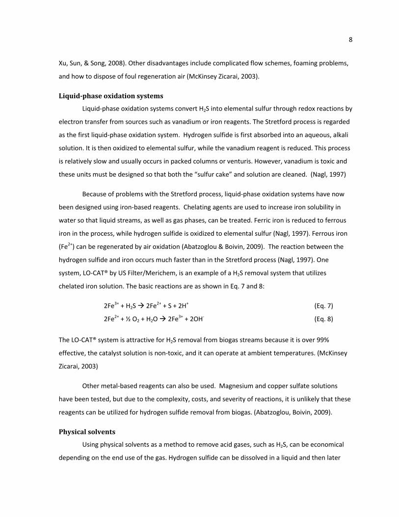
Liquid-phase oxidation systems
Liquid-phase oxidation systems convert H2S into elemental sulfur through redox reactions by
electron transfer from sources such as vanadium or iron reagents. The Stretford process is regarded
as the first liquid-phase oxidation system. Hydrogen sulfide is first absorbed into an aqueous, alkali
solution. It is then oxidized to elemental sulfur, while the vanadium reagent is reduced. This process
is relatively slow and usually occurs in packed columns or venturis. However, vanadium is toxic and
these units must be designed so that both the “sulfur cake” and solution are cleaned. (Nagl, 1997)
Because of problems with the Stretford process, liquid-phase oxidation systems have now
been designed using iron-based reagents. Chelating agents are used to increase iron solubility in
water so that liquid streams, as well as gas phases, can be treated. Ferric iron is reduced to ferrous
iron in the process, while hydrogen sulfide is oxidized to elemental sulfur (Nagl, 1997). Ferrous iron
(Fe2+) can be regenerated by air oxidation (Abatzoglou & Boivin, 2009). The reaction between the
hydrogen sulfide and iron occurs much faster than in the Stretford process (Nagl, 1997). One
system, LO-CAT® by US Filter/Merichem, is an example of a H2S removal system that utilizes
chelated iron solution. The basic reactions are as shown in Eq. 7 and 8:
2Fe3+ + H2S � 2Fe2+ + S + 2H+ (Eq. 7)
2Fe2+ + ½ O2 + H2O � 2Fe3+ + 2OH- (Eq. 8)
The LO-CAT® system is attractive for H2S removal from biogas streams because it is over 99%
effective, the catalyst solution is non-toxic, and it can operate at ambient temperatures. (McKinsey
Zicarai, 2003)
Other metal-based reagents can also be used. Magnesium and copper sulfate solutions
have been tested, but due to the complexity, costs, and severity of reactions, it is unlikely that these
reagents can be utilized for hydrogen sulfide removal from biogas. (Abatzoglou, Boivin, 2009).
Physical solvents
Using physical solvents as a method to remove acid gases, such as H2S, can be economical
depending on the end use of the gas. Hydrogen sulfide can be dissolved in a liquid and then later

9
removed from the liquid by reducing the pressure. For more effective removal, liquids with higher
solubility for H2S are used. However, water is widely available and low-cost. Water washing is one
example of a physical solvent-utilizing process. Water also has solubility potential for CO2, and
selective removal of just H2S has not proved economical using water. (McKinsey Zicarai, 2003)
Other physical solvents that have been used are methanol, propylene carbonate, and ethers
of polyethylene glycol. Criteria for selecting a physical solvent are high absorption capacity, low
reactivity with equipment and gas constituents, and low viscosity. One problem with using physical
solvents is that a loss of product usually occurs, due to the pressure changing processes necessary to
later remove the H2S from the solvent. Losses as high as 10% have been found. (McKinsey Zicarai,
2003).
Membrane processes
Membranes can be used to purify biogas. Partial pressures on either side of the membrane
control permeation through the membrane. Membranes are not usually used for selective removal
of H2S, and are rather used to upgrade biogas to natural gas standards. There are two types of
membrane systems: high pressure with gas phase on both sides of the membrane, and low pressure
with a liquid adsorbent on one side. In one case, cellulose acetate membranes were used to upgrade
biogas produced by anaerobic digesters. (McKinsey Zicarai, 2003)
Biological methods
Microorganisms have been used for the removal of H2S from biogas. Ideal microorganisms
would have the ability to transform H2S to elemental sulfur, could use CO2 as their carbon source
(eliminating a need for nutrient input), could produce elemental sulfur that is easy to separate from
the biomass, would avoid biomass accumulation to prevent clogging problems, and would be able to
withstand a variety of conditions (fluctuation in temperature, moisture, pH, O2/H2S ratio, for
example). Chemotrophic bacterial species, particularly from the Thiobacillus genus, are commonly
used. Chemotrophic thiobacteria can be used both aerobically and anaerobically. They can utilize
CO2 as a carbon source and use chemical energy from the oxidation of reduced inorganic
compounds, such as H2S. In both reactions, H2S first dissociates:
H2S ↔ H+ + HS- (Eq. 9)
Under limited oxygen conditions, elemental sulfur is produced:

10
HS- + 0.5O2 → S0 + OH- (Eq. 10)
Under excess oxygen conditions, SO42- is produced, which leads to acidification:
HS- + 2O2 → SO42- + H+ (Eq. 11)
One chemotrophic aerobe, Thiobacillus ferroxidans, removes H2S by oxidizing FeSO4 to
Fe2(SO42-)3, and then the resulting Fe3+ solution can dissolve H2S and chemically oxidize it to
elemental sulfur. These bacteria are also able to grow at low pH levels, which make them easy to
adapt to highly fluctuating systems. (Abatzoglou & Boivin, 2009)
Biological H2S removal can be utilized in biofilter and bioscrubber designs. One commercially
available biological H2S removal system is Thiopaq®. It uses chemotrophic thiobacteria in an alkaline
environment to oxidize sulfide to elemental sulfur. It is able to simultaneously regenerate hydroxide,
which is used to dissociate H2S. Flows can be from 200 Nm3/h to 2,500 Nm3/h and up to 100% H2S,
with outlet concentrations of below 4 ppmv. (Abatzoglou & Boivin, 2009)
Another system, H2SPLUS SYSTEM®, uses both chemical and biological methods to remove
H2S. A filter consisting of iron sponge inoculated with thiobacteria is used. There are about 30
systems currently in use in the U.S., mostly at agrifood industry wastewater treatment plants. Gas
flows of 17 to 4,200 m3/h can be used, and removal capacity is up to 225 kg H2S/day. (Abatzoglou &
Boivin, 2009)
Materials Used for H2S Adsorption
Various materials are used as adsorbents for hydrogen sulfide. These materials have specific
surface properties, chemistry, and other factors that make them useful as H2S adsorbents. A study
by Yan, Chin, Ng, Duan, Liang, and Tay (2004) about mechanisms of H2S adsorption revealed that H2S
is first removed by physical adsorption onto the liquid water film on the surface of the adsorbent,
then by the dissociation of H2S and the HS- reaction with metal oxides to form sulfides, then with
alkaline species to give neutralization products, and finally with surface oxygen species to give redox
reaction products (such as elemental sulfur). If water is not present, CO2 can deactivate the alkaline-
earth-metal-based reaction sites and lead to lower H2S removal. Additionally, the oxidation
reactions of H2S are faster when Ca, Mg, and Fe are present, as they are catalysts for these reactions
(Abatzoglou & Boivin, 2009). Physical adsorption also occurs in pores, and pores between the size of

11
0.5 and 1 nm were found by Yan et al. to have the best adsorption capacity. Significant adsorption
occurs when a material is able to sustain multiple mechanisms. The materials described in this
section have been shown to utilize one or more of these mechanisms and have shown potential as
H2S adsorbent materials.
Activated carbon
Activated carbons are frequently used for gas adsorption because of their high surface area,
porosity, and surface chemistry where H2S can be physically and chemically adsorbed (Yuan &
Bandosz, 2007). Much of the research has focused on how the physical and chemical properties of
various activated carbons affect the breakthrough capacity of H2S. Most activated carbon tested is
in granular form, called Granular Activated Carbon (GAC). Activated carbon can come in two forms:
unimpregnated and impregnated. Impregnation refers to the addition of cations to assist as
catalysts in the adsorption process (Bandosz, 2002). Unimpregnated activated carbon removes
hydrogen sulfide at a much slower rate because activated carbon is only a weak catalyst and is rate-
limited by the complex reactions that occur. However, using low H2S concentrations and given
sufficient time, removal capacities of impregnated and unimpreganted activated appear to be
comparable in laboratory tests. Removal capacities may vary greatly in on-site applications, as the
presence of other constituents (such as VOCs) may inhibit or enhance the removal capacity,
depending on other environmental conditions (Bandosz, 2002). The cations added to impregnated
activated carbon are usually caustic compounds such as sodium hydroxide (NaOH) or potassium
hydroxide (KOH), which act as strong bases that react with H2S and immobilize it. Other compounds
used to impregnate activated carbons are sodium bicarbonate (NaHCO3), sodium carbonate
(Na2CO3), potassium iodide (KI), and potassium permanganate (KMnO4)(Abatzoglou & Boivin, 2009).
When caustics are used, the activated carbon acts more as a passive support for the caustics rather
than actively participating in the H2S removal because of its low catalytic ability. The caustic addition
has a catalytic effect by oxidizing the sulfide ions to elemental sulfur until there is no caustic left to
react. The reactions that unimpregnated activated carbon undergoes to facilitate H2S removal is far
less understood (Bandosz, 2002). A typical H2S adsorption capacity for impregnated activated
carbons is 150 mg H2S/g of activated carbon. A typical H2S adsorption capacity for unimpregnated
activated carbons is 20 mg H2S/g of activated carbon. (Abatzoglou & Boivin, 2009)

12
Much research has focused on mechanisms of H2S removal using activated carbon. A
researcher from the Department of Chemistry in the City College of New York, Teresa Bandosz, has
performed numerous studies on the adsorption of H2S on activated carbons (Bandosz, 2002; Adib,
Bagreev, & Bandosz, 2000; Bagreev & Bandosz, 2002; Bagreev, Katikaneni, Parab, & Bandosz, 2005;
Yuan & Bandosz, 2007). Her studies have focused on hydrogen sulfide adsorption on activated
carbons as it relates to surface properties, surface chemistry, temperature, concentration of H2S gas,
addition of cations, moisture of gas stream, and pH. These experiments have used both biogas from
real processes and laboratory produced gases of controlled composition.
In a study by Bagreev and Bandosz (2002), NaOH impregnated activated carbon was tested
for its H2S removal capacity. Four different types of activated carbon were used and different
volume percentages of NaOH were added. The results showed that with increasing amounts of
NaOH added, the H2S removal capacity of the activated carbons increases. This effect occurred until
maximum capacity was reached at 10 vol% NaOH. This result was the same regardless of the origin
of the activated carbon, and was even the same when activated alumina was used. This result
implies that the amount of NaOH present on the surface of the material is a limiting factor for the
H2S removal capacity in NaOH impregnated activated carbons.
Although impregnated activated carbon can be an effective material for the adsorption of
H2S, there are a few drawbacks of using this material. First, the addition of caustics lowers the
ignition temperature and therefore the material can self-ignite and is considered hazardous.
Secondly, the addition of caustics to activated carbon increases the costs of production. Lastly,
because of the high cost of activated carbon, it is desirable to “wash” or “clean” the activated
carbon in order to regenerate it so that it will regain some of its ability to remove H2S (Calgon
Carbon Corp., a leading producer of activated carbon, priced an unimpregnated activated carbon
used in wastewater treatment applications to be $8.44/lb and impregnated activated carbon is even
more expensive). One of the simple ways to regenerate the activated carbon is to wash it with
water. The caustic additions to impregnated activated carbon cause H2S to be oxidized to elemental
sulfur, which cannot be removed from the activated carbon by washing with water and therefore
costs of H2S removal are increased due to the need to purchase more adsorbent. (Bandosz, 2002)
As of yet, the complete mechanisms by which H2S is removed using activated carbon are not
well understood. It is accepted that removal occurs by both physical and chemical mechanisms. One

13
chemical removal mechanism is caused by the presence of heteroatoms at the carbon surface.
Important heteroatoms are oxygen, nitrogen, hydrogen, and phosphorus. They are incorporated as
functional groups in the carbon matrix and originate in the activated carbon as residuals from
organic precursors and components in the agent used for chemical activation. They are important in
the chemical removal of H2S because they influence the pH of the carbon, which can control which
species (acidic, basic, or polar) are chemisorbed at the surface. Another important factor in H2S
removal has been the presence of moisture on the carbon surface. Bandosz has a theory that, in
unimpregnated activated carbon, H2S will dissociate in the film of water at the carbon surface and
the resulting sulfide ions (HS-) are oxidized to elemental sulfur (Bandosz, 2002). Bandosz found that
the activated carbon’s affinity for water should not be greater than 5%, otherwise the small pores of
the adsorbent become filled by condensed adsorbate and the direct contact of HS- with the carbon
surface becomes limited. It was found that some affinity for water adsorption was desirable in an
adsorbent. However, when biogas is used at the source of H2S, it is not practical to optimize the
amount of water on the media because biogas is usually already water saturated. Too much water
can interfere with the H2S removal reactions because the water in gaseous form reacts with CO2 to
form carbonates and contributes to the formation of sulfurous acid which can deactivate the
catalytic sites and reduce the capacity for hydrogen sulfide to react and be removed (Abatzoglou &
Boivin, 2009).
Bandosz and her research group have focused considerably on the mechanisms of H2S
removal on unimpregnated activated carbon. In Adib, Bagreev, & Bandosz (2000) it was found that
as oxidation occurs on the surface of the carbons, the capacity for adsorption decreases. The
adsorption and immobilization of H2S was found to be related to its ability to dissociate and this was
inhibited by the oxidized surface of the activated carbons. No relationship between pore structure
and adsorption ability was found, but it was noted that a higher volume of micropores with small
volumes enhances the adsorption capacity. The most important finding of this study was that the pH
of the surface has a large affect on the ability of H2S to dissociate. Acidic surfaces (<5) decrease the
H2S adsorption capacity of the activated carbons.
The concentration of H2S in the inlet gas may affect the adsorption capacity of activated
carbons. One study indicated that the H2S removal capacity of impregnated activated carbons
increases when the H2S concentration decreases (Bagreev et. al, 2005). In the same study, it was

14
also found that small differences in oxygen content (1-2%) and different temperatures (from 38°C-
60°C) did not have a significant effect on the hydrogen sulfide removal. In another study, it was
found that adsorption capacities of H2S on impregnated activated carbon slightly decrease with
increasing temperature (30 and 60°C were tested). (Xiao, Ma, Xu, Sun, & Song, 2008)
The effect of low H2S concentration on removal capacity can be explained by the fact that
the low concentration slows down oxidation kinetics, which in turn slows down the rate of surface
acidification. Surface acidification has been shown to be detrimental to H2S removal because H2S
does not dissociate readily in acidic conditions (Abatzoglou & Boivin, 2009).
Zeolites (Molecular sieves)
Zeolites, also commonly referred to as molecular sieves, are hydrated alumino-silicates
which are highly porous and are becoming more commonly used to capture molecules. The size of
the pores can be adjusted by ion exchange and can be used to catalyze selective reactions (McCrady,
1996). The pores are also extremely uniform. Zeolites are especially effective at removing polar
compounds, such as water and H2S, from non-polar gas streams, such as methane (McKinsey Zicarai,
2003). Current research is focusing on how to implement zeolites in “clean coal” technology, or
Integrated Gasification Combined Cycle (IGCC) power plants. Some studies about the use of zeolite-
NaX and zeolite-KX as a catalyst for removing H2S from IGCC gas streams have been performed at
Yeungnam University in Korea. One study found a yield of 86% of elemental sulfur on the zeolites
over a period of 40 hours (Lee, Jun, Park, Ryu, & Lee, 2005). Gas streams from IGCC power plants
are at a high temperature, between 200 and 300°C. Further, molecular sieves have recently been
used as a structural support for other types of adsorbents (Wang, Ma, Xu, Sun, & Song, 2005).
Polymers
There has not been significant research done using polymers as adsorbents for H2S, but a a
study was found where polymers were used in conjunction with other materials to enhance
adsorption. This study, by Wang et al. (2008), studied the effects on H2S adsorption of adding
various compositions of a polymer, polyethylenimine (PEI), to a molecular sieve base. The
mesoporous molecular sieves tested were amorphous silicates with uniform mesopores. PEI was
deposited on the samples in varying compositions of 15-80 wt% of the molecular sieve. The results
showed that the lower temperature tested (22°C) had higher sorption capacity, a loading of 50 wt%
PEI on the molecular sieves had the best breakthrough capacity, and that a loading of 65 wt% PEI

15
had the highest saturation capacity. Additionally, the sorbents can easily be regenerated for
continued H2S adsorption. The authors suggest that H2S adsorbs onto the amine groups of the PEI,
and at low compositions of PEI on the molecular sieves the amines present may be reacting with
acidic functional groups on the molecular sieve surface. At high compositions of PEI on the
molecular sieves, the surface area of the molecular sieve was significantly decreased and because
the adsorption and diffusion rates of H2S depend on surface area, the H2S was not able to be
effectively adsorbed.
Metal oxides
Metal oxides have been tested for hydrogen sulfide adsorption capacities. Iron oxide is
often used for H2S removal. It can remove H2S by forming insoluble iron sulfides. The chemical
reactions involved in this process are shown in the following equations:
Fe2O3 + 3H2S � Fe2S3 + 3H2O (Eq. 12)
Fe2S3 + 3/2O2 �Fe2O3 +3S (Eq. 13)
Iron oxide is often used in a form called “iron sponge” for adsorption processes. Iron sponge
is iron oxide-impregnated wood chips. Iron oxides of the forms Fe2O3 and Fe3O4 are present in iron
sponge. It can be regenerated after it is saturated, but it has been found that the activity is reduced
by about one-third after each regeneration cycle (Abatzoglou & Boivin, 2009). Iron sponge can be
used in either a batch system or a continuous system. In a continuous system, air is continuously
added to the gas stream so that the iron sponge is regenerated simultaneously. In a batch mode
operation, where the iron sponge is used until it is completely spent and then replaced, it has been
found that the theoretical efficiency is approximately 85% (McKinsey Zicarai, 2003). Iron sponge has
removal rates as high as 2,500 mg H2S/g Fe2O3. Some challenges associated with the use of iron
oxide for hydrogen sulfide removal from biogas are that the process is chemical-intensive, there are
high operating costs, and a continuous waste stream is produced that must either be expensively
regenerated or disposed of as a hazardous waste. There are some commercially produced iron oxide
based systems that are able to produce non-hazardous waste. One commercially available iron oxide
base system, Sulfatreat 410-HP® was found to have an adsorption capacity of 150 mg H2S/g
adsorbent through lab and field-scale experiments. (Abatzoglou & Boivin, 2009)

16
The iron sponge is a widely used and long-standing technology for hydrogen sulfide removal.
Because of this, there are accepted design parameters for establishing an H2S removal system.
Table 2 summarizes these design parameters.
Table 2, Iron sponge design parameter guidelines (McKinsey Zicarai, 2003)
Design Parameter Guidelines
Vessels Stainless-steel box or tower geometries are recommended for ease of
handling and to prevent corrosion. Two vessels, arranged in series are
suggested to ensure sufficient bed length and ease of handling.
Gas Flow Down-flow of gas is recommended for maintaining bed moisture. Gas
should flow through the most fouled bed first.
Gas Contact Time A contact time of greater than 60 seconds, calculated using the empty bed
volume and total gas flow, is recommended.
Temperature Temperature should be maintained between 18°C and 46°C in order to
enhance reaction kinetics without drying out the media.
Bed Height A minimum 3 m bed height is recommended for optimum H2S removal. A 6
m bed is suggested if mercaptans are present.
Superficial Gas Velocity The optimum range for linear velocity is reported as 0.6 to 3 m/min.
Mass Loading Surface contaminant loading should be maintained below 10 g S/min/m2.
Moisture Content In order to maintain activity, 40±15% moisture content is necessary.
pH Addition of sodium carbonate can maintain pH between 8 and 10. Some
sources suggest addition of 16 kg sodium carbonate/m3 of sponge initially
to ensure an alkaline environment.
Pressure While not always practiced, 140 kPa is the minimum pressure
recommended for consistent operation.
The iron sponge costs around $6/bushel (approx. 50 lbs) from a supplier, but other
technologies that utilize iron sponge, such as the Model-235 from Varec Vapor Controls, Inc., can
cost around $50,000 for the system and initial media (McKinsey Zicarai, 2003).
Other metal oxides besides iron oxide have been used to remove hydrogen sulfide. Carnes
and Klabunde (2002) found that the reactivities of metal oxides depend on the surface area,
crystallite size, and intrinsic crystallite reactivity. It was found that nanocrystalline structures have
better reactivity with H2S than microcrystalline structures, high surface areas promote higher
adsorption, and high temperatures are ideal (but not higher than the sintering temperature,
otherwise a loss of surface area occurs). Also, the presence of Fe2O3 on the surface furthers the
reaction. The reason proposed for this was that H2S reacts with the Fe2O3 to form iron sulfides that
are mobile and able to seek out the more reactive sites on the core oxide and exchange ions, and
ultimately acts as a catalyst in the reaction. However, at ambient temperatures this effect is not as

17
clearly seen. In the study, calcium oxide was the most reactive (and with additions of surface Fe2O3
it was even more reactive), followed by zinc oxide, aluminum oxide, and magnesium oxide. In one
study, Rodriguez and Maiti (2000) found that the ability of a metal oxide to adsorb H2S depends on
the electronic band gap energy: the lower the electronic band gap energy, the more H2S is adsorbed.
This is because the electronic band gap is negatively correlated to the chemical activity of an oxide
and the chemical activity depends on how well the oxide’s bands mix with the orbitals of H2S. If the
bands mix well, then the oxide has a larger reactivity towards the sulfur-containing molecules, and
metal sulfides are created, which cause H2S molecules to dissociate and the sulfur to be immobilized
in the metal sulfides. Use of metal oxides for hydrogen sulfide removal can have problems such as
low separation efficiency, low selectivity, high costs, and low sorption/desorption rate.
Zinc oxides are used to remove trace amounts of H2S from gases at high temperatures (from
200°C to 400°C), because zinc oxides have increased selectivity for sulfides over iron oxides
(McKinsey Zicarai, 2003). Davidson, Lawrie, and Sohail (1995) studied hydrogen sulfide removal on
zinc oxide and found that the surface of zinc oxide reacts with the H2S to form an insoluble layer of
zinc sulfide, thereby removing H2S from a gas stream. Approximately 40% of the H2S present was
converted over the ZnO adsorbent. The reaction described in Equation 14 leads to H2S removal:
ZnO + H2S �ZnS + H2O (Eq. 14)
Various commercial products use zinc oxide, and maximum sulfur loading on these products is
typically in the range of 300 to 400 mg S/g sorbent (McKinsey Zicarai, 2003).
Sludge derived adsorbents
Because many commercially available adsorbents of H2S are costly or have other associated
problems, attention has been given to using various sludge derived materials as adsorbents. When
sludge undergoes pyrolysis, a material is obtained with a mesoporous structure and an active
surface area with chemistry that may promote the oxidation of hydrogen sulfide to elemental sulfur
(Yuan & Bandosz, 2007). The mechanisms of H2S removal described by Yan et al. (2004) can be
applied to sludge derived adsorbents. Sludge has a complex chemistry, but it has enough of the
reactive species given by Yan et al. that it could provide an alternative to using non-impregnated
activated carbon. The efficiency of sludge at H2S removal has been found to be similar to that of iron
based adsorbents, but less efficient than impregnated activated carbon (Abatzoglou & Boivin, 2009).
18
A concern with using sludge is that it may contain compounds which adversely affect H2S removal.
Some compounds in question are derived from metal sludge produced by industry. A study by Yuan
and Bandosz (2007) mixed various weights of sewage sludge and metal sludge derived from a
galvanizing process used in industry, pyrolyzed them, and tested them for hydrogen sulfide
adsorption capacity. It was found that the capacity for H2S adsorption is comparable to the capacity
of impregnated activated carbons, and that the adsorption capacity depends on the overall sludge
composition and the pyrolysis temperature. Samples with higher content of sewage sludge
pyrolyzed at higher temperatures (800°C and 950°C) had the best adsorption capacity. The highest
adsorption capacity reported was less than 21 mg H2S/g adsorbent, which is less than the adsorption
capacity of unimpregnated activated carbon.
Methods of Controlling Siloxane Emissions
Siloxanes must be removed from biogas before it is combusted in order to avoid silica
particle formation. Some methods of siloxane removal are similar to hydrogen sulfide removal.
Chemical abatement
Chemical abatement is a reactive extraction process using contact between gas and liquids
to facilitate the reactions. In chemical abatement, the Si-O bond in the siloxane molecule is broken.
This reaction is catalyzed by strong acids such as HNO3 and H2SO4. Alkalis can be used but there is
the disadvantage that CO2 is also retained, which increases the quantity of chemicals used and thus
drives up the cost of treatment. (Abatzoglou & Boivin, 2009)
Adsorption
Activated carbon, molecular sieves, and silica gel have been investigated for use as an
adsorbent for siloxanes. Adsorptive capacity has been found to depend on the type of siloxane
present, where D5 has been found to adsorb better than other types of siloxanes. Silica gel can be
an effective adsorbent, but the gas must be dried in order for maximum removal capacities to be
achieved. The maximum removal capacity of silica gel has been found to be around 100 mg
siloxane/g of silica gel. Silica gel can be regenerated, but the removal capacity decreases. Activated
alumina and iron-based adsorbents have also been found effective at removing siloxanes.
(Abatzoglou & Boivin, 2009)

19
Absorption
Siloxanes are soluble in some organic solvents with high boiling points, such as tetradecane.
These solvents can absorb siloxanes in spray or packed columns. Tetradecane has been found to
have a 97% removal efficiency of D4 siloxane. However, this method is costly and is not
economically feasible in small- to medium-scale facilities. (Abatzoglou & Boivin, 2009)
Cryogenic condensation
It has been found that freezing to temperatures of -70°C is necessary to remove more than
99% of siloxanes. At these low temperatures, siloxanes will condense and can be separated from
the gas phase. It was found that at 5°C, 88% of siloxanes are still in the gas phase and at -25°C, 74%
of siloxanes are still in the gas phase. Because of the extremely low temperatures needed for
effective siloxane removal, this method is not feasible for small- to medium-scale facilities.
(Abatzoglou & Boivin, 2009)
Particles Derived from Waste Rubber Products
This research utilizes waste rubber products, called tire derived rubber particles (TDRP) and
other rubber materials (ORM). TDRP and ORM are produced and distributed by Envirotech Systems,
Inc. The process by which TDRP is produced is proprietary, but information is available about other
frequently used types of particles derived from used tires.
Particles from used tires
Approximately 281 million tires were discarded in the United States in 2001. This constitutes
that, on average, there is one tire discarded every year for every person in the United States. There
are applications that these tires, in various forms, can be used. Many of these applications require
the tires be in a form called “crumb rubber”. Crumb rubber can generally be defined to be particle
sizes of 3/8-inch or less. Crumb rubber can be classified into four groups:
1) Large or coarse (3/8”-1/4", or 9.525-6.350 mm),
2) Mid-range (10-30 mesh, 0.079”-0.039”, or 2.000-1.000 mm),
3) Fine (40-80 mesh, 0.016”-0.007”, or 0.406-0.178 mm), and
4) Superfine (100-200 mesh, 0.006”-0.003”, or 0.152-0.076 mm)
It is difficult to generalize particle size requirements in each market for crumb rubber, and therefore
it is a challenge for crumb producers. However, rough estimates indicated that demand for the

20
various sizes described are about 14% for coarse sizes, 52% for mid-range sizes, 22% for fine sizes,
and 12% for superfine sizes. (Sunthonpagasit & Duffey, 2004)
Applications of rubber particles from used tires
Crumb rubber is used in various applications, and its use and demand has been increasing.
Figure 1 shows the increase of crumb rubber utilization since 1994.
Figure 1, Scrap tire utilization (Sunthonpagasit & Duffey, 2004)
The largest application of used tires is tire derived fuel, where it is used as a supplemental fuel in
cement kilns. This application accounts for approximately 33% of total scrap tires generated.
Shredded rubber can be used in civil engineering applications, such as leachate collection in landfills
and for highway embankments. These applications account for approximately 15% of scrap tires
generated. Crumb rubber generation accounts for about 12% of scrap tires generated. Applications
of crumb rubber include asphalt modification, molded products, sport surfacing, plastic blends, tires
and automotive products, surface modification, animal bedding, and construction applications.
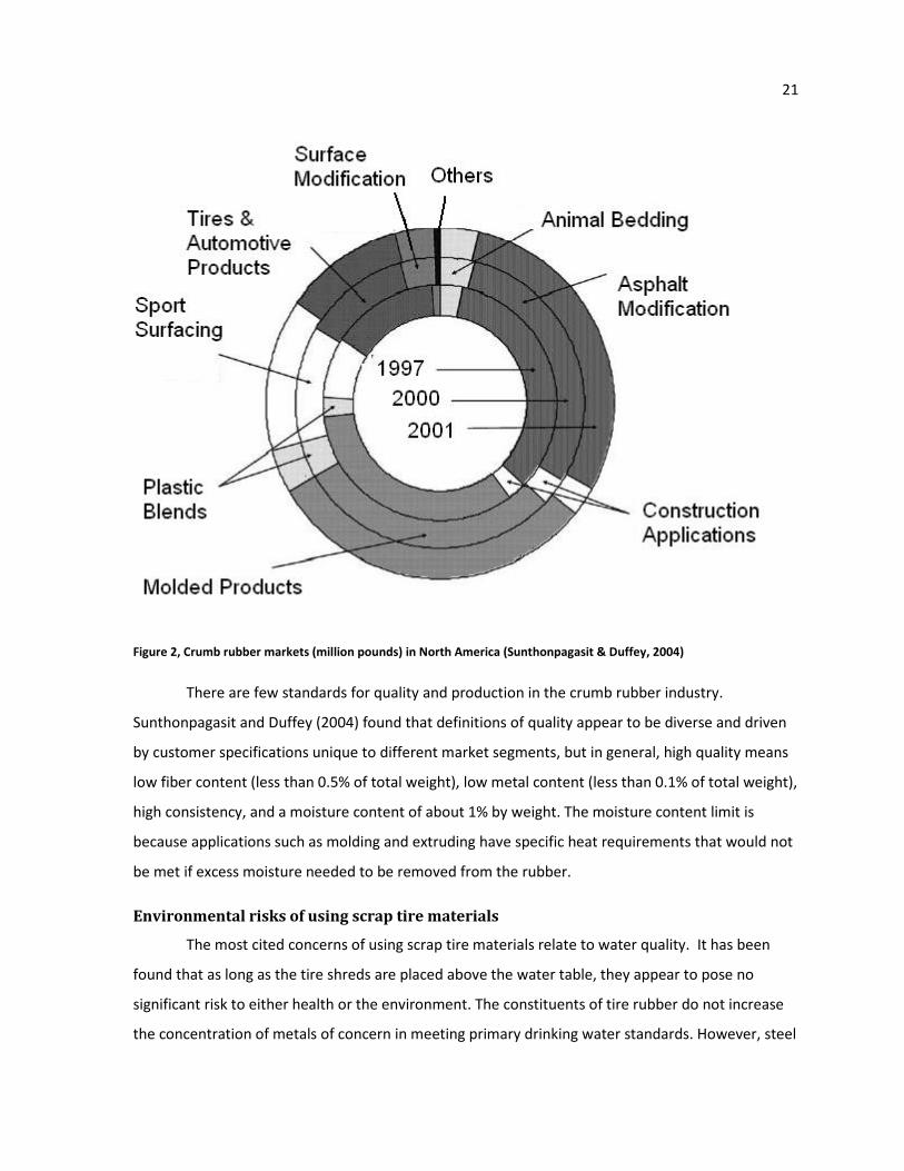
Figure 2 describes the growing demand for crumb rubber in various applications from 1997 to 2001.
(Sunthonpagasit & Duffey, 2004)
21
Figure 2, Crumb rubber markets (million pounds) in North America (Sunthonpagasit & Duffey, 2004)
There are few standards for quality and production in the crumb rubber industry.
Sunthonpagasit and Duffey (2004) found that definitions of quality appear to be diverse and driven
by customer specifications unique to different market segments, but in general, high quality means
low fiber content (less than 0.5% of total weight), low metal content (less than 0.1% of total weight),
high consistency, and a moisture content of about 1% by weight. The moisture content limit is
because applications such as molding and extruding have specific heat requirements that would not
be met if excess moisture needed to be removed from the rubber.
Environmental risks of using scrap tire materials
The most cited concerns of using scrap tire materials relate to water quality. It has been
found that as long as the tire shreds are placed above the water table, they appear to pose no
significant risk to either health or the environment. The constituents of tire rubber do not increase
the concentration of metals of concern in meeting primary drinking water standards. However, steel

22
belts are exposed at the cut edges of the tire shreds, which may increase the levels of iron and
manganese, affecting secondary drinking water standards. (Sunthonpagasit & Duffey, 2004.)
There may also be issues with worker exposure to fine respirable particles and particle-
bound polycyclic aromatic hydrocarbons (PAHs). One study of road paving workers using crumb
rubber modified asphalt found potential exposure to “elevated airborne concentrations of a group
of unknown compounds that likely consist of the carcinogenic PAHs benz(a)anthracene, chrysene
and methylated derivatives of both.” (Sunthonpagasit & Duffey, 2004)
Crumb rubber production
The process of crumb rubber production can vary with end-use applications. However,
Sunthonpagasit and Duffey (2004) generalize the process of producing 3/8” (9.525 mm) to 80 mesh
(0.178 mm) crumb rubber particles in Figure 3:
Figure 3, Generalized crumb rubber production (Sunthonpagasit & Duffey, 2004)
23
Crumb production processes occur at ambient temperatures in the majority of production
operations. Most operations separate passenger car and truck tire processing. In the production
process, after tires are first separated into truck and passenger car tires, the tires are de-rimmed
and shredded and/or granulated to a mesh size of approximately 3/8” (9.525 mm) or 5-30 mesh.
The 3/8” (9.525 mm) product has about 5% metal and the 5-30 mesh product has about 0.1% metal.
These products can either be sold as-is or reduced to smaller sizes, depending on the application.
After granulation, the process to produce smaller mesh sizes is referred to as the “powder process”.
The amount of rubber waste following each process is 8% for shredding, 6% for granulating, and 4%
for the powder process. (Sunthonpagasit & Duffey, 2004)
Other production considerations include the type of processing equipment that is needed
and the condition of the processing equipment. As truck tires usually have large amounts of
reinforcing wires in them, they are more difficult to process and therefore require different
processing equipment than that needed for passenger car tires. The condition of the processing
equipment also plays a significant role in the quality of the product and in the maintenance costs
associated with processing. (Sunthonpagasit & Duffey, 2004)
Tire characteristics
On average a passenger car tire is equivalent to about 20 lbs. Each passenger car tire
contains approximately 86.0% rubber compound, 4% fiber, and 10% metal. Truck tires are about
100 lbs and contain approximately 84.5% rubber compound, less than 0.5% fiber, and 15 % metal.
The composition of the processed tires will change somewhat, due to processing techniques such as
magnetic metal removal, which also removes rubber particles that are attached to the ferrous
metals. (Sunthonpagasit & Duffey, 2004)
Tires are made of vulcanized rubber and other reinforcing materials. Vulcanized rubber is a
polymer with cross-linked chains. The reinforcing materials include fillers and fibers. Fillers are
generally made of carbon black, which strengthens the rubber and provides abrasion resistance.
Fibers are made of textiles or steels, usually in the form of a cord, which provide strength and a
tensile component. The rubber compound in the tires is generally of the composition listed in Table
3.

24
Table 3, Rubber compound composition (Amari et al., 1999)
Component Mass %
Styrene-butadiene 62.1
Carbon black 31.0
Extender oil 1.9
Zinc oxide 1.9
Stearic acid 1.2
Sulfur 1.1
Accelerator 0.7
Total 99.9
Organo-sulfur compounds, zinc oxide, and stearic acid are used as vulcanizing agents.
Styrene-butadiene (SBR) is a co-polymer most commonly used as the rubber matrix. Sometimes it is
a blend of natural rubber and SBR. Extender oil is usually petroleum oil which is used to control
viscosity, reduce internal friction during processing, and improve low temperature flexibility in the
vulcanized product. The accelerator aids in vulcanization. (Amari, Themelis, & Wernick, 1999)
Characteristics of TDRP and ORM
The TDRP and ORM were previously characterized in a past study (Ellis, 2005) using sieve
analyses and a chemical analysis. Figure 4 and Figure 5 show sieve analyses of ORM and TDRP
performed as part of this study. These sieve analyses show that ORM has a well balanced spread of
particle sizes over a larger range of sizes. On the other hand, TDRP has more of the material over a
smaller range of sizes.
Figure 4, Sieve analysis of ORM for 2 samples (Ellis, 2005)
0%10%20%30%40%50%60%70%80%90%
100%
0.1 1 10
Wt.
% P
assi
ng
Sieve Size (mm)
A-2
A-1

25
Figure 5, Sieve analysis of TDRP for 2 samples (Ellis, 2005)
A chemical analysis performed in the same study found that TDRP and ORM contained zinc,
magnesium, chlorine, sulfur, silicon, calcium, and oxygen. Information was not available about
concentrations and specific differences between TDRP and ORM. Information provided by
Envirotech Systems, Inc. said that TDRP had “metal additions” and ORM did not, but no specific
information was available. TDRP is shown in Figure 6.
Figure 6, TDRP at a magnification of 1.5X
0%
10%
20%
30%
40%
50%
60%
70%
80%
90%
100%
0.1 1 10
Wt.
% p
assi
ng
Sieve Size (mm)
B-2
B-1
26
Experimental Methods
Because tire particles have not been used in H2S removal applications, there is no existing
literature about experimental methods. Experimental methods for H2S removal from literature were
referred to as a basis for creating an experimental method and apparatus for testing the tire
particles.
ASTM: D 6646-03. Standard Test Method for Determination of the Accelerated Hydrogen
Sulfide Breakthrough Capacity of Granular and Pelletized Activated Carbon
The American Society for Testing and Materials, ASTM International, provides a standard
regarding the testing of the breakthrough capacity of GAC. This method is for virgin, newly
impregnated or in-service, granular or pelletized activated carbon with a mean particle diameter less
than 2.5 mm meant to remove hydrogen sulfide from an air stream. Although this standard provides
accepted methodology for activated carbon, it is not necessarily applicable to non-carbon
adsorptive materials.
This method defines breakthrough of the activated carbon to be when the outlet gas stream
of an activated carbon bed has a concentration of 50 ppmv H2S when the inlet concentration is
10,000 ppmv H2S. It is emphasized that this test does not simulate actual conditions encountered in
real-life situations and is only meant to compare the breakthrough of different carbons. One of the
reasons is that the column size, 23 cm, has a mass transfer zone that is proportionally much larger
than the typical bed used in practical application and causes carbons with rapid kinetics for H2S
removal to be favored over carbons with slower kinetics.
The recommended gas used in this method is nitrogen with controlled H2S concentrations.
The H2S sensor should be able to reliably detect 50 ppm, and either “solid state” or electrochemical
type sensors are suggested. The media bed is located in an adsorption tube, which has specific
dimensions as shown in Figure 7.

27
Figure 7, Schematic of adsorption tube (ASTM, 2003)
A way of controlling the flow of gas is needed. It is recommended that a flow meter, mass
flow controller, or rotameter with corrosion resistant parts be used with the potential of measuring
flow rates of 0-2,000 mL/min nitrogen. A source of dry, contaminant-free air capable of delivering
up to 2 L/min is needed to mix with the H2S to the desired concentration, 10,000 ppm (1 vol%) H2S.
Also needed are: an air line pressure regulator to maintain up to 10 psig pressure for up to 2 L of
air/min, two metering valves, a gas bubbler to ensure the generation of a 80% relative humidity air
stream, H2S calibration gas, and a timer. The entire schematic should be similar to Figure 8.

28
Figure 8, Schematic of apparatus for determination of H2S breakthrough capacity (ASTM, 2003)
To run the system, the H2S/N2 system should first be adjusted to produce a 10,000 ppm H2S
stream at a total flow rate of 1,450 cm3/min. For the media bed, 116 mL of carbon should be used.
It should be placed in the bed using a vibratory feeder. The system should be run until an outlet
concentration of 50 ppmv H2S is reached. (ASTM, 2003)
The main calculation derived from this test is the H2S breakthrough capacity of the GAC in g
H2S/cm3 GAC. The calculation is as follows, assuming standard conditions:
� ������� � �100� � � � � � 1 �1000 ���� � 1 ����22.4 � � � �34.1 � ������� ��
(Eq. 15)
where: C = concentration of H2S in air stream, volume %
F = total H2S/air flow rate, cm3/min
T = time to 50 ppmv breakthrough, min and
V= actual volume of the carbon bed in the absorption tube, cm3
The apparent density of the GAC can then be used to convert this into units of g H2S/g GAC.
According to the standard the sample average and standard deviation are calculated, and if the

29
standard deviation is within 10% of the average, it can be reported as the H2S breakthrough
capacity. (ASTM, 2003)
This system is the closest standard that exists for H2S removal in an adsorptive bed. This
experimental method is very strictly controlled and is meant to be used in a laboratory environment.
Other experimental systems
The literature available about H2S removal onto an adsorbent describes various laboratory-
controlled experiments with various experimental parameters. A few of these experiments are
reviewed here.
The relative humidity is usually 70% or 80%. The temperature of the gas is held around 25°C
or slightly higher. Inlet concentrations of H2S are usually varied throughout the course of the
experiment to establish isotherms, and are usually incremented between 1,000 ppmv and 5,000
ppmv. The dimensions of the reaction column differ slightly between studies, but are generally
about 200-400 mm in length, either 8-9 mm or much larger, such as 2.5 cm-6.5 cm in diameter, and
15 to 23 cm in bed height. These dimensions are often structured around the ASTM standard,
depending on the adsorbent being used. Flow rates are from 0.12 L/min to 0.5 L/min. The
temperature inside the column is controlled, and a temperature of about 25°C is often used, but
sometimes elevated temperatures, such as 60°C are used. The contact time in the scrubber depends
on both the volume of the media bed and the flow rate, but was found to be either very small, on
the order of 0.5 s, or much higher, such as 30 or 60 seconds. The experiments are generally stopped
when a certain concentration of H2S is detected in the outlet gas. These concentrations are from 10
ppm to 500 ppm. (Bandosz, 2002; Bagreev et al., 2005; Xiao, Wang, Wu, & Yuan, 2008; Truong &
Abatzoglou, 2005; and Yuan & Bandosz, 2007)
Of course, these parameters are varied depending on the scope of the experiment, and it is
difficult to generalize a H2S adsorption experiment.

30
CHAPTER 3. THEORY
Adsorption
Adsorption is a process used to remove undesirable compounds in gas or liquid streams by
passing the stream through a media bed composed of a solid material. The solid material used is
called the adsorbent and the gas or liquid compound being adsorbed is called the adsorbate. In
adsorption, the adsorbate penetrates into the pores of the adsorbent, but not into the lattice itself
(Davis & Cornwell, 2008). Only gas streams were used in this research project and therefore this
review will henceforth only apply to gas streams. The adsorption process can be used to dehumidify
gas, remove odors or pollutants from the stream, or recover valuable solvent vapors from the
stream. Adsorption has been found to be particularly applicable to gas that is noncombustible or
difficult to burn, pollutants that are valuable when recovered, and pollutants that are in very dilute
concentrations (Wark, Warner, & Davis, 1998).
The mechanisms of adsorption are either physical or chemical. In physical adsorption,
intermolecular forces cause the gas molecules to be attracted to and adhere to the surface of the
adsorbent. The adsorption process is always exothermic, and the amount of heat released depends
on the magnitude of the attractive force but is usually between 2 and 20 kJ/g·mol. Physical
adsorption is usually reversible by either lowering the pressure of the adsorbate in the gas stream or
raising the temperature, which makes regenerating and reusing the spent adsorbent possible.
Because physical adsorption involves the adherence of gas molecules to the surface of the
adsorbent, the adsorption capacity is directly proportional to the surface area of the adsorbent.
However, the adsorbent is not limited to a single layer of molecules on the surface; multiple layers
of adsorbate molecules may accumulate. In chemical adsorption, or chemisorption, a chemical
reaction occurs between the adsorbate and the adsorbent. The chemical reactions that occur in
chemisorption have much stronger bonds than the physical attractive forces in physical adsorption,
on the range of 20 to 400 kJ/g·mol. Chemisorption is usually not reversible and only a single layer of
adsorbate molecules may be present on the surface because the valence force adhering the
adsorbate to the adsorbent are only effective over extremely short distances. (Wark et al., 1998)
A material used as an adsorbent must have certain properties in order to be an effective
adsorbent. Particle diameters can range from about 1.3 cm to less than 200 μm and the material

31
should have a high surface area per unit weight ratio. Some materials that are effective adsorbents
have extremely high surface area per unit weight ratios due to the surface area of internal pores on
the solid. If the pore diameter is a few times larger than the molecular diameter of the adsorbate,
the pores will be readily available for adsorption. Another advantageous property of the adsorbent
is if it has a chemical affinity for the adsorbate. Materials commonly used for adsorption were
discussed in depth in the Literature Review. (Wark et al., 1998)
An adsorption system should be designed with respect to the properties of both the
adsorbent and the adsorbate. Some requirements for an adsorption system identified by Wark et al.
are the provision for sufficient dwell time, the pretreatment of the gas stream to remove non-
adsorbable matter and remove high concentrations of competing gases, good distribution of flow
through the bed, and a provision of regenerating the adsorbent bed after saturation. Sufficient dwell
time (contact time) is necessary so that the physical and/or chemical reactions have time to occur. It
is necessary to remove non-adsorbable matter because it may impair the operation of the
adsorbent bed. Similarly, it is important to remove high concentrations of competing gases so that
the system does not get overburdened and become ineffective at removing the pollutant of
concern. Operation of a system can be in either a batch or continuous mode and may involve a
regenerative process. Generally, if the pollutant is on the order of 1 to 2 ppm or less, the adsorbent
is discarded rather than regenerated. However, this is also dependent on the nature of the pollutant
and whether it is highly volatile once adsorbed. If continuous operation is used, it is common to
have two beds in parallel so that one can be regenerating (or being replaced) while the other is
being used for adsorption. (Wark et al., 1998)
Adsorption isotherms are useful tools for modeling adsorption behavior. An adsorption
isotherm relates the volume or mass adsorbed to the partial pressure or concentration of the
adsorbate in the gas stream at a constant temperature. Experimental adsorption data has shown
that increasing the pressure of the adsorbate in the gas stream causes a higher amount to be
adsorbed. Increases in temperature of adsorption systems have been found to decrease the amount
adsorbed, and therefore it is usually desirable to operate an adsorption system at as low a
temperature as possible. Additionally, it has been found that adsorption improves with an increase
in the molar mass of the adsorbate. (Wark et al., 1998)

32
Various theories have been developed to describe experimental adsorption behavior. The
most common theoretical models are the Langmuir Isotherm, the Brunauer-Emmett-Teller (B.E.T.)
Model, and the Freundlich Isotherm. The Langmuir Isotherm assumes that adsorption occurs on a
fixed number of sites that are all energetically equivalent, each site can adsorb only one molecule,
and interactions between adsorbed molecules are neglected because they are assumed to be small
compared to the interaction between the adsorbate and the adsorbent (Keller & Staudt, 2005). The
Langmuir isotherm is described in Eq. 16,
�� ! � 1" # $" �� (Eq. 16)
where W is the amount of gas per unit mass of adsorbent (kg/kg), Cg* is the equilibrium
concentration of gaseous pollutant (g/m3), and a and b are constants which are experimentally
determined (Davis & Cornwell, 2008). The Langmuir model was chosen as one of the isotherms to
model the experimental data.
The B.E.T. Model is an extension of the Langmuir Isotherm and it describes multiple layers of
molecules that are adsorbed on the surface of an adsorbent. The B.E.T. equation (Eq. 17), which is
associated with this model, is based on the rates of condensation and evaporation from the layers of
molecules on the surface of the adsorbent:
��% � �&�&' ( &�)1 # �� ( 1� &&'�* (Eq. 17)
where V is the volume of adsorbed gas would fill at a given temperature and pressure, Vm is the
volume adsorbed if a layer one molecule thick fills the surface, P0 is the vapor pressure of the
adsorbate at the system temperature, P is the actual partial pressure of the adsorbate in the gas
stream, and c is a parameter associated with the adsorption process. Vm and c are determined
experimentally. Research has found that the B.E.T. equation may be difficult to evaluate if values of
P/P0 are less than 0.05 or greater than 0.35. (Wark et al., 1998)
The Freundlich Isotherm is another type of isotherm used to describe the adsorption of a
single layer of molecules onto an adsorbent. It is commonly used to fit experimental data. It is
described in Eq. 18:

33
�+ � ,-./01 (Eq. 18)
where Ce is the equilibrium concentration of the pollutant with the adsorbent, Xsat is the saturated
adsorbent concentration, and α and β are experimentally determined constants. The Freundlich
isotherm was also used to model data in this research because of its simplicity and ability to
successfully model experimental data. (Wark et al., 1998)
As the pollutant moves through the media bed, some is adsorbed onto the adsorbent
located closest to the inlet gas. When that part of the adsorbent bed becomes saturated with the
adsorbate, it cannot adsorb any more of the adsorbate and the adsorption process continues with
the adsorbent located next to it. This continues down the length of the media bed. In this manner,
the adsorption of the adsorbate onto the adsorbent can be said to occur in a “wave”, as shown in
Figure 9.
Figure 9, Adsorption wave (Wark, Warner, & Davis, 1998)
Figure 9 shows the velocity of the adsorption wave, Vad, through the bed of depth Db. At point x1
along the length of the bed, the bed up until x1 is completely saturated with adsorbate
(concentration of adsorbate on the adsorbent is Xsat and concentration of adsorbate in the main gas
stream is the inlet concentration, C0). At point x2, which is farther from the inlet gas than x1, the bed
does not have any adsorbate adsorbed on it (concentration, C, is zero). The difference in length
from points x1 to x2 is δ, which is known as the width of the adsorption zone, and is where the active
adsorption processes are occurring. When point x2 reaches point Db, the concentration of the
pollutant in the outlet gas will begin to increase and “breakthrough” will occur in the bed. When

34
point x1 reaches Db the adsorbent bed will be completely saturated with the adsorbate and the
outlet pollutant concentration will be the same as the inlet pollution concentration.
Assuming behavior consistent with the Freundlich Isotherm and using a mass balance on the
pollutant in the adsorption zone, an equation can be derived describing the velocity of the
adsorption wave as
�/2 � �3 /4/4/2 ,5/1�7�185�/1 (Eq. 19)
where �3 / is the mass flow rate of the carrier gas, ρa is the density of the carrier gas, ρad is the
apparent bulk density of the adsorbent, A is the area of the bed cross-section, C0 is the inlet
concentration of H2S, and α and β are constants, as described in Eq. 18 (Wark et al., 1998). Because
this equation is based on an isotherm, the α and β constants are temperature dependent. For the
current adsorption system, the carrier gas is the biogas, the adsorbent is the TDRP, and the inlet
concentration C0 can be assumed to be equivalent to the equilibrium concentration, Ce, described in
Eq. 18.
To find the width of the adsorption zone, δ, further relationships between concentration
and distance in the media bed (x) can be derived. Wark et al. (1998) describes in detail the process
of deriving these relationships. Equation 20 shows the relationship of δ to concentration as a result
of some of these derivations. In Eq. 20, η represents the ratio of concentration to inlet
concentration of the adsorbate in the main gas stream (C/C0):
9:4/�3 / � ; <==�1 ( =185�5'
(Eq. 20)
where K is a film coefficient for the transfer process that takes into account the film resistance as
well as the effective interfacial area of the adsorbent. The integral in Eq. 5 is undefined at the
boundaries of η=0 and η=1, but using values close to these boundaries will allow the integral to be
evaluated. Wark et al. uses boundaries of η=0.01 to η=0.99, which is the same as defining an
adsorption zone width such that C approaches within 1% of its limiting values of 0 and C0. Evaluating
the integral at these boundaries, substituting equivalent terms, and defining the adsorption zone
width to be x2-x1 gives Eq. 21, which describes the shape of the concentration versus distance curve:

35
> � >5 # �3 /:4/ ?�@ 0.99�'� # 1B ( 1 �@ 1 ( � ��'�1851 ( �0.99�185C
(Eq. 21)
Different values of η can be chosen, depending on the acceptable limit of pollutant in the outlet gas
(there are different definitions of when breakthrough occurs).
The time of breakthrough can be predicted using Eq. 22 if δ is known and if it is assumed
that the time required to establish the full width of the adsorption zone at the inlet is zero:
DE � FG ( 9�/2 (Eq. 22)
Combining Eq. 19 and 22 gives an expression for the volume of media needed:
�FG ( 9� � �3 /DE4/4/2 ,5/1�7�185�/1 (Eq. 23)
Application of Theory to Experimental Data
As previously mentioned, the Freundlich isotherm (Eq. 18) was used to model the
experimental data in this study. The use of Eq. 18 requires values for Ce, the equilibrium
concentration of the adsorbate with the adsorbent, and Xsat, the saturated adsorbent concentration.
The equilibrium concentration, Ce, was assumed to be the inlet adsorbate concentration because
this study used a continuous adsorption system instead of a batch system. The inlet adsorbate
concentration was found experimentally by averaging the inlet pollutant concentration before
breakthrough occurred. The saturated adsorbent concentration was assumed to be the amount of
adsorbate removed from the inlet gas up until the time of breakthrough. Figure 10 shows an
example of a breakthrough curve from this study. Every hour, a sample of both the inlet and outlet
gases from the system was taken. The amount of adsorbate (H2S in this study) removed from the
inlet gas up until the time of breakthrough was determined with this experimental data by
converting the H2S concentration to mg of H2S per gram of TDRP (the adsorbent), then integrating
the area between the inlet and outlet curves.

36
Figure 10, Example of a breakthrough curve from the study
Integration of the curves was performed using the trapezoid method. The trapezoid method
approximates the area under a curve by averaging the height of 2 consecutive points on the curve
and multiplying it by the horizontal distance between the 2 points. This is shown graphically in
Figure 11.
Figure 11, Graphical representation of the trapezoid method for integrating a curve (Trapezoidal Rule, 2010)
0
50
100
150
200
250
300
350
0 500 1000 1500 2000 2500 3000 3500 4000
H2S
Co
nce
ntr
ati
on
, p
pm
Time, min
Inlet
Outlet

37
In the case of Figure 10, both the inlet curve and the outlet curve were integrated up until the point
of breakthrough using the trapezoid method, then the value obtained for the outlet curve was
subtracted from the value obtained for the inlet curve. This area between the inlet and outlet curves
represents the amount of H2S removed from the inlet stream by the TDRP, and is therefore a close
approximation of the value of Xsat.
Equation 18 can be manipulated to yield Eq. 24:
log ��+� � log�,� # Blog �-./0� (Eq. 24)
Experimental data was used for Ce and Xsat. A linear trendline was fit to the resulting plot. From this
trendline, α and β were determined (α was found by equating log(α) to the y-intercept of the linear
line and β was the slope of the line). Once α and β were determined, they were applied to Eq. 23.
As noted, Eq. 23 gives an expression for the volume of media needed using the media bed length Db,
the width of the adsorption zone δ, and the area A. Because δ is difficult to determine from
experimental data due to its relatively small value, δ was assumed to be zero for the purpose of
practical calculations. By assuming δ to be zero, the calculated length of the media bed, Db, is the
length of the bed needed for complete saturation to occur. By applying a safety factor (SF) to the
volume of calculated media needed, sudden (and possibly catastrophic) breakthrough is avoided.
Applying this to Eq. 23 gives Eq. 25.
���K�� � �� · FG � �� · �3 /DE4/4/2 ,5/1�7�185�/1 (Eq. 25)
This theory lays the groundwork for the calculations that follow in the Results section.

38
CHAPTER 4. MATERIALS AND METHODS
Experimental Apparatus
Gas flow through system
The experimental apparatus was set-up and maintained at the WPCF in the Gas Handling
Building. A schematic of the scrubber system is shown in Figure 12.
Figure 12, Schematic of scrubber system

39
As shown in Figure 12, the biogas from the anaerobic digesters at the WPCF entered the
system and first passed through a check valve to prevent any backflow from entering the gas
handling system. The gas was then either sampled by the H2S detector if the solenoid controller
opened the solenoid valve, or continued to pass through an isolation valve and rotameter and into
the scrubber. The isolation valve was used to shut off gas flow to the system if necessary and the
rotameter was used to control the flow through the system. The scrubber was temperature
controlled by the temperature control system. The temperature control system pumped water
through copper tubes that were wound around the outside of the scrubber and then insulated.
Once the gas entered the scrubber, it passed through the media bed. The pressure difference in the
scrubber could be read from manometers located both at the inlet and outlet sides of the scrubber.
Two different thermometers were located in the scrubber. One was a data logging thermocouple,
which recorded a temperature reading every 30 seconds. The other was a dial thermometer, which
was used to corroborate the readings from the thermocouple and also when the data logging
thermometer was not properly functioning. There was also a gas sample port located on the
scrubber and a drainage valve underneath it to remove condensation.
After the gas passed through the media bed, it flowed out of the scrubber and then could be
sampled by the H2S detector through the solenoid valve. It then passed through another isolation
valve and a flame arrestor as safety precautions. The outlet gas was exhausted outside the Gas
Handling Building.
An air source was also attached to the H2S detector. This was controlled by the solenoid
controller, and it was run in between inlet and outlet gas sampling times in order to stabilize the
detector. The gas being sampled or run through the H2S detector also was exhausted outside the
Gas Handling Building.
The actual set-up of the scrubber system is shown in Figure 13. Figure 13 depicts the acrylic
scrubber housing and all related appurtenances and controls. The system was designed to split the
flow of the biogas into two scrubbers so that simultaneous experiments could be run. However, the
flow of biogas through the system was not enough to divide between two scrubbers and only one of
the scrubbers was utilized in this study (the scrubber seen on the left).

40
Figure 13, Scrubber system
Figure 14 shows the system with the addition of the temperature control system. The scrubber that
was utilized for experiments was insulated after copper tubing carrying temperature controlled
water was wrapped around it. Parts of the system are labeled in Figure 14, as shown in the
schematic in Figure 12. For scale, the rotameter on the left side of the table is 10.2 cm tall.
Figure 14, Scrubber system with the addition of the temperature control system

41
Scrubber dimensions
The height of the screen supporting the media bed to the top lip of the scrubber was 53.5
cm. The media bed was generally 4,000 mL in volume and was approximately 42 cm in height. The
diameter of the scrubber was 11.4 cm.
Temperature control system
As previously mentioned, the temperature control system consisted of a temperature
controlled water supply, which was pumped into copper tubes that wrapped around the scrubber.
The entire scrubber was also insulated. The temperature control system was used to test
temperatures as low as 30°F (-1°C) and as high as 170°F (77°C). It should be noted that these
temperatures are the temperature of the water supply. The actual temperature in the scrubber did
not reach these temperatures. The data logging thermocouple measured the actual temperature in
the scrubber during different trials.
The temperature control system was not added until Trial 16 of the experiments. It was at
this time that the effect of temperature was to be studied and some method of changing the
temperature inside the scrubber was necessary. Despite the lack of a temperature control system
prior to Trial 16, the temperature in the scrubber remained fairly constant. This is primarily due to
the location of the system in the Gas Handling Building. The Gas Handling Building contained
engines which ran at peak hours to generate electricity from the biogas. The running of the engines
created a fairly stable ambient temperature in the building. However, the system was also located
next to a window in the Gas Handling Building. When outside temperatures reached extremes, it
affected the temperature in the scrubber despite the use of a temperature control system.
Hydrogen sulfide detector
A Jerome® 860 hydrogen sulfide detector produced by Arizona Instrument LLC (Tempe, AZ)
was used. The Jerome® 860 was a portable gas monitor that could continuously collect data and
then transfer it to a computer or pocket PC via an infrared USB port. It was battery powered, water
resistant, and safe. The detector used an electro-chemical sensor to measure H2S concentrations. It
was recommended that the measurement range be between 0 and 200 ppm, however the detector
was able to handle occasional spikes in the H2S concentration up to 1,000 ppm. The resolution of the
detector was 0.2 ppm. It was recommended that the temperature of the measured gas be between
0°C and 50°C and the humidity of the gas be 20 to 80% for normal operation, but could reach 100%

42
for short intervals. Oxygen was required for the sensor to operate properly, so between samples air
was pumped through the sensor. (Arizona, 2005)
In high humidity and high temperature environments, it was recommended that the sensor
be removed from operation every 2 days to allow the sensor to stabilize (Arizona, 2005). In the case
of this experiment, the sensor was used for the entire 2.5 day time period for each trial. After the
trial was complete, the sensor was removed from the system and air was run through the sensor
until the next trial commenced.
Two-minute samples of gas from the inlet and outlet were taken every hour. An H2S
concentration was recorded every 2 seconds. The H2S detector had the capacity to record 108,810
readings. In each trial, the system was run until the capacity of the H2S detector was reached, which
was about 2.5 days (60.5 hours).
Data logging thermocouple
The data logging thermocouple used was a ThermoWorks® (Lindon, UT) brand USB data
logger (TW-USB-TC). It took a temperature reading from inside the scrubber every 30 seconds. The
data logging thermocouple appeared to function correctly until Trial 19. It was then determined that
the temperatures being recorded were inconsistent with the actual temperatures in the scrubber by
comparing temperature readings from a dial thermometer in the scrubber. The data logging
thermocouple was then sent back to the manufacturer and was replaced. The new data logging
thermocouple was reinstalled and functioning correctly by Trial 26. During the time period where
the data logging thermocouple was not available, temperature was recorded daily from the dial
thermometer and averaged over the length of the experiment.
Rotameter
The rotameter used was manufactured by Omega Engineering, Inc. (Stamford, CT) and had
the capability of measuring flows between 1 to 10 L/min of air at 0.5 L/min intervals. A correction
for using biogas instead of air was used when calculating the actual flow rate of biogas through the
system. Because of the specific gravity of the biogas, the correction of the biogas flow rate was
calculated to be 1.0426 times the reading of the rotameter.

43
Solenoid controller
The solenoid controller used was a model XT manufactured by ChronTrol Corporation (San
Diego, CA). This controller could be programmed to control four solenoid valves. In the program for
the controller used, 3 solenoid valves for taking samples of gas at various stages in the system and
one air pump for stabilizing the detector were controlled. Because the scrubber system was initially
designed for using 2 separate scrubbers, there are 3 solenoid valves built into the system for
sampling gas: one to sample the inlet gas, and two to sample outlet gas from each of the two
scrubbers. However, because only one scrubber was utilized in the actual study due to low biogas
flow rates, only samples from two of the solenoid valves were used. A visual describing the program
for the solenoid controller is shown in Figure 15.
Figure 15, Solenoid controller program for a 60 minute cycle
In Figure 15, Solenoid 1 refers to the valve controlling sample gas from the inlet, Solenoid 2 controls
the flow of sample gas from the first scrubber, and Solenoid 3 controls the flow of sample gas from
the second scrubber. The air pump is energized during the times indicated and is only on when gas is
not being sampled. The cycle was repeated every 60 minutes.
Flame Arrestor
The flame arrestor used was a Varec 5200 Flame Check, manufactured by Varec Biogas
(Cypress, CA). A flame arrestor is designed to stop flashbacks in small pipe lines carrying flammable
gases. It is recommended to be installed as close as possible to the open end of the pipe, where it is
more likely a source of flame will originate. A flame arrestor extinguishes any flashbacks that are
generated by passing it through a compressed woven wire element which absorbs heat from the

44
flame faster than it is developed. The temperature is thus lowered below its ignition point and the
flame is quenched.
Experimental Procedure
Material collection and measurement
TDRP and ORM were collected and weighed in Town Engineering Building on the Iowa State
University campus. For almost all trials, 4,000 mL of TDRP was used. It was collected using a 4,000
mL beaker. The TDRP was manually mixed and large clumps were dispersed. The TDRP mass was
then measured on a Model CW-11 floor scale manufactured by Ohaus Corporation (Pine Brook, NJ)
and calibrated linearly with a zero point and a span point of 20 kg (subtracting the mass of the
beaker, 0.32 kg); the scale was setup for a capacity of 100 kg with graduated increments of 0.02 kg.
It should be noted that until Trial 10, the floor scale was not functional and there was no means of
massing the TDRP. The masses of the TDRP prior to Trial 10 were estimated, depending on the
method of collecting the media (mixing and sifting versus no additional mixing or sifting) and the
bulk density of the TDRP.
Preparation of the experimental apparatus
The TDRP or ORM was poured into the top of the scrubber. A line was marked on the
scrubber (see Figure 13) to show how high 4,000 mL of TDRP generally filled the scrubber. The bed
height of the media was measured by measuring the distance from the top lip of the scrubber to the
top of the bed and then subtracting it from the distance of the bottom of the media bed to the top
lip (21-1/6”, or 53.5 cm). Any spilled TDRP was wiped off the top of the scrubber and vacuum grease
was applied around the seal at the top. The lid of the scrubber was put in place, and the bolts were
secured.
The data logging thermocouple was activated by connecting it to a computer via a USB port
and using the software, EasyLog USB, to begin recording. The H2S detector first needed to be
calibrated in the labs at Town Engineering Building. Calibration gas of 200 ppm was most often used,
but concentrations of 25 ppm and 10 ppm were also used. After calibration, the data already stored
in the detector was cleared. The detector was then ready for data collection.
A system check was then performed to ensure that the appropriate valves were opened or
closed and that the H2S sensor and data logging thermocouple were recording.
45
Beginning and running the experiment
After the system was checked, it was ready to begin an experiment. The gas was turned on.
The flow rate through the system was controlled by the rotameter. To maintain a constant flow rate,
it was found that a flow rate of 3 L/min or less resulted in a relatively flat system curve over the
pressure range encountered. For most trials, a flow rate of 3 L/min was applied. Some trials focused
on changing the empty bed contact time and these trials required different flow rates. The pressure
in the line from the digester was recorded, as well as the inlet and outlet pressures from the
manometers, the temperature from the dial thermometer, and the flow through the system.
After initial set-up and beginning of the experiment, the experiment was monitored on a
daily basis. Pressure in the line from the digester was recorded, as well as the pressures from the
manometers on the inlet and outlet end of the scrubber, temperature from the dial thermometer,
and flow rate.
Occasionally, condensation in some of the plastic tubing was present. This was usually due
to a temperature difference in the gas and the temperature control system. The tubes containing
condensation were drained during the experiment to ensure that the water was not causing
blockages.
Ending the experiment
After collecting approximately 2.5 days of data, the H2S detector memory was exhausted
and would automatically turn off. The data was then downloaded from both the H2S detector and
the data logging thermocouple. The scrubber was unsealed after the gas was shut off and the media
was removed and disposed.
Siloxane Testing
Siloxane testing was conducted on inlet and outlet gas from the scrubber in order to
evaluate the siloxane removal capability of TDRP (ORM was not evaluated for siloxane removal).
Siloxane concentrations were measured concurrent with hydrogen sulfide testing. A small sample of
inlet and outlet gases was drawn from the lines; no effect on flow was observed.
The methods described by Air Toxics (Saeed, Kao , & Graening, 2002) were used for siloxane
sampling and analysis of type D4 (Octamethyl-Cyclotetrasiloxane) and type D5 (Decamethyl-

46
Cyclopentasiloxane) siloxanes. Results are reported as the sum of D4 and D5 siloxanes. The specific
methods and equipment for this test are described in Appendix II.
Site Variables
There are a number of variables that control the site conditions for this study. A brief
explanation of each variable can be found below.
Flow Rate of Biogas
The flow rate of the biogas through the system was controlled by the pressure at the gas tap
of the anaerobic digesters. The pressure varied between 14”-16” at the gas tap which, after losing
some pressure head along the line to the experimental apparatus, gave a maximum flow of between
3-6 L/min. The flow of the gas through the system was controlled by a rotameter (up to the
maximum flow) which was connected to the scrubber. The original research plan indicated that a
flow of 2.7 cubic feet/min (76.5 L/min) would be used, but this flow was scaled back to meet site
specific conditions.
The flow rate of the biogas and the height of the media bed determine the residence time,
or empty bed contact time. Using a full bed of media (defined as 4,000 mL and explained further
below), the empty bed contact time varied from around 60 seconds to around 500 seconds.
Amount of Media
The amount of media used was measured volumetrically. For a “full bed” in the scrubber,
4,000 mL of media was used. This volume of media gives a mass of between 1,340 to 1,580 grams. A
few of the trials used a “half-bed” of media, which was 2,000 mL of TDRP.
Type of Media
There were two types of waste rubber materials available for use in this study. From
knowledge passed on from Envirotech, Inc., ORM contained slightly coarser particles and no metal
additions. TDRP was finer and had metal additions, supposedly from the steel belts of the discarded
tires. A previous study showed that iron, calcium, zinc, and magnesium were present in TDRP, but
the exact quantities were unknown. Additional characterization of TDRP and ORM from a previous
study can be found in the Literature Review section. Most of the experiments in this study focused
on using TDRP. However, there were 5 trials performed at the end of the study using ORM.
47
Traditionally, activated carbon or steel wool is used as an adsorbent for hydrogen sulfide in
similar applications. As a comparison, two experiments were done using steel wool as the media and
one experiment was run as a blank, using marbles as an inert surface for the gas to pass through.
Compaction of Media
TDRP is capable of being significantly compacted. Most of the experiments used TDRP in its
loose, natural form, with no additional compaction other than from the weight of itself. However, a
few trials focused on the effects of compacting the media. The method of compaction was to apply
pressure at the top of the bed using manual force and then placing glass marbles on top of the
media to prevent it from expanding. In the compaction trials, the bed was compacted to up to 66%
of its original volume.
Temperature
The temperature of the gas in the system was primarily a function of the temperature of the
gas leaving the anaerobic digesters or the temperature inside the Gas Handling Building. When the
temperature control system was not in operation, the temperature inside the scrubber appeared to
be a function of time and ran in a daily, cyclical cycle that did not necessarily correlate with the
weather (day vs. night).
Concentration of the Inlet Gas
The concentration of the biogas from the anaerobic digesters varied. It was usually between
250-300 ppm, but got as high as 1,600 ppm and as low as 60 ppm. There were sometimes drastic
drops in the concentration that appeared to correlate with fat, oil, and grease (FOG) deliveries from
a large local restaurant, Hickory Park. It was not possible to control inlet concentration. A value that
has been developed to characterize the amount of hydrogen sulfide loading to the scrubber is the
mg of H2S present in the gas per gram of TDRP present in the media bed per hour. The Results
section contains a plot of H2S concentrations from all experiments over the course of approximately
10 months (Figure 20).
Pressure
The atmospheric pressure is used to calculate the amount of hydrogen sulfide removed. The
atmospheric pressure is slightly variable, but is usually very close to 1 atm. The values used for
atmospheric pressure are taken from the Weather Underground (www.wunderground.com).

48
CHAPTER 5. RESULTS AND DISCUSSION
Hydrogen Sulfide Testing
Various operational conditions were tested to determine their effect on the hydrogen
sulfide (H2S) concentration of the outlet gas. The following conditions were tested:
• Empty bed contact time
• Temperature of the biogas and scrubber media
• Compaction of the media bed
• Mass of TDRP used in the media bed
Two different types of waste rubber materials were used from Envirotech Systems, Inc.: tire derived
rubber particles (TDRP) and other rubber materials (ORM). Most of the experimental testing on
different operational conditions was done using TDRP. ORM was only tested at a single empty bed
contact time, temperature, compaction (density), and mass.
A typical breakthrough curve from this study is shown in Figure 10. Breakthrough occurred
when the H2S concentration in the outlet gas began to increase. In this section, two different time
periods are referred to: the time from the start of the experiment until the point of breakthrough,
and a fixed period of time for all experiments that was from when the experiment began until it was
ended, and always exceed the time until breakthrough.
Empty bed contact time
Empty bed contact time was varied by adjusting flow to the scrubber using a rotameter
equipped with a needle valve. A longer contact time was found to slightly increase the amount of
H2S removed up until the time of observed breakthrough, although the total amount of H2S
removed throughout the duration of the experiment was not found to be dependent on the contact
time. This suggests that there was a maximum amount of H2S that could be removed by the TDRP
particles as a result of thermodynamic limitations. To overcome kinetic limitations, a longer contact
time resulted in greater H2S removal prior to reaching maximum removal capacity. These findings
can be seen in Figure 16.

49
As a statistical analysis, F-tests which tested the research hypothesis that the slope of the
trendline, β, was 0 were performed. These F-tests tested the null and research hypotheses as listed
in Eq. 26.
�7: B � 0 NO. �/: B P 0 (Eq. 26)
Two F-tests were performed. The first F-test tested whether there was a trend in the data
for the amount of H2S adsorbed from the starting time of the experiment up until the point of
breakthrough. The second F-test tested whether there was a trend in the data for the amount of
H2S adsorbed from the starting time of the experiment until the end of the experiment, which was a
fixed amount of time for all experiments.
For the first F-test, the trend of H2S removed at breakthrough was found to be statistically
significant (see Table 4 for results of statistical tests), meaning that the research hypothesis that the
slope was 0 was rejected at α=0.25. On the other hand, the second F-test found that the H2S
removed over a fixed period of time did not vary as a function of empty bed contact time; i.e. fail to
reject the hypothesis that the slope is zero (Table 4). Therefore, there was not a trend over this data
and there was evidence that the empty bed contact time did not change the total amount, which
included H2S adsorbed after breakthrough, of H2S adsorbed over an extended period of time. The p-
values of the statistical tests can be used to test significance under different values for α. If the p-
value is less than the chosen α-value, it is a good indication that the null hypothesis can be rejected
at that α-value.
Table 4, Statistical test results for empty bed contact time
Data F-test R2 Fc F0.25,1,4 p-value
Adsorbed until breakthrough #1 0.72 10.2 1.81 0.03
Adsorbed over fixed time #2 0.12 0.56 1.81 0.49

50
Figure 16, Effect of empty bed contact time on H2S removed at breakthrough and over a fixed time period
Appendix I contains the complete data set for the trials that are associated with Figure 16.
Temperature
The effect of temperature on adsorption was tested. Figure 17 shows the relationship
between temperature in the scrubber and the total amount of H2S removed over a fixed period of
time. Low temperatures were tested by setting the temperature control system to 30°F (-1°C).
Medium temperatures were tested either at ambient temperatures (which was around 75°F (24°C)
in the Gas Handling Building) before the temperature control system was installed, or after it was
installed the temperature control system was set to 75°F (24°C). High temperatures were tested by
setting the temperature control system to 170°F (77°C).
In the tests performed, low temperatures appeared to have the highest H2S removal
capacity; however, the data did not identify a significant effect of temperature. The low correlation
(R2=0.0046) of this trendline signified the lack of a trend between temperature and H2S removal
capacity. A statistical F test for determining whether the slope of the trendline was zero concluded
that there was no evidence that there was a linear trend among the data (Table 5). Kohl and Nielsen
(1997) indicate that the adsorption process is always exothermic, and therefore adsorption capacity
decreases with increasing temperature. This may be the correct trend for TDRP and the relatively
small amount of H2S removed at medium temperatures could be due to the lower concentrations of
H2S in the inlet gas. The average inlet H2S concentration for the medium temperature trials was 355
y = 0.0014x + 0.4055
R² = 0.7201
0.00
0.20
0.40
0.60
0.80
1.00
1.20
1.40
0 100 200 300 400 500 600
mg
H2S
/g T
DR
P
Empty bed contact time, s
Adsorbed at
breakthrough
Adsorbed over
fixed time
period

51
ppm, whereas the average inlet H2S concentration for the low temperature, which exhibit higher
removal capacities, was 637 ppm. Figure 21 shows the trend between inlet H2S concentration
(described as H2S loading) and H2S removal capacity. Because the H2S removal capacity appeared to
be lower at higher temperatures, this indicated that kinetics was not a limiting factor for the
reaction between the H2S and TDRP and therefore an increase in temperature, which would
increase the kinetic rate of reaction, was not beneficial in achieving maximum H2S removal. This
indicated that the equilibrium between H2S and TDRP, instead of the kinetics, governed H2S removal
from biogas using TDRP as the adsorbent. However, there was not a large difference in the
temperatures that were tested, and the effect of temperature may not be clearly seen in the range
of temperatures that were used. Future tests on much higher or lower temperatures, if possible,
could yield a significant trend.
Table 5, Statistical test results for temperature effect
Data R2 Fc F0.25,1,10 p-value
Temperature 0.0046 0.06 1.49 0.82
Figure 17, Effect of temperature on the amount of H2S removed over a fixed time period
Appendix I contains the complete data set for the trials that are associated with Figure 17.
Compaction
The effect of compaction on the media bed was tested. The same initial mass of TDRP was
used (approximately 1.4 kg) in each test. After being placed in the scrubber, the bed was compacted
y = -0.0075x + 2.3303
R² = 0.00440.00
1.00
2.00
3.00
4.00
5.00
6.00
0 10 20 30 40 50 60H2S
re
mo
ve
d o
ve
r a
fix
ed
tim
e p
eri
od
,
mg
H2S
/g T
DR
P
Temperature, °C
Low Temp
Mid Temp
High Temp

52
to approximately 65% of the volume of the original bed in both trials (from 4,000 mL to 2,600 mL).
The results show that, in general, compaction improved adsorption capacity (Figure 18). The
trendline gave an R2 value of 0.432. A statistical F test for determining whether the slope of the
trendline is zero concluded that there was evidence that there was a linear trend among the data
(Table 6). It was hypothesized that the improved capacity resulted from reduced biogas short-
circuiting. The average H2S removed with compaction was 1.89±0.45 mg/g TDRP, whereas the
average removed without compaction was 1.13±0.05 mg/g TDRP.
Table 6, Statistical test results for compaction effect
Data R2 Fc F0.25,1,10 p-value
Compaction 0.432 3.80 1.69 0.109
Figure 18, Bed compaction effects on amount of H2S removed
Appendix I contains the complete data set for the trials that are associated with Figure 18.
Mass of media bed
Reducing the mass of the media bed decreased the amount of H2S that was removed on a
mass of sulfur per mass of TDRP basis. This is shown in Figure 19, where the flow rate was the same
for both the full bed (4,000 mL) and half bed (2,000 mL) trials and the density was maintained at its
uncompacted density.
y = -0.0254x + 3.3207
R² = 0.4301
0.00
0.50
1.00
1.50
2.00
2.50
3.00
0 20 40 60 80 100
H2S
re
mo
ve
d o
ve
r a
fix
ed
tim
e p
eri
od
,
mg
H2S
/g T
DR
P
Empty bed contact time, s
Bed compaction
(~35% reduction)
No compaction
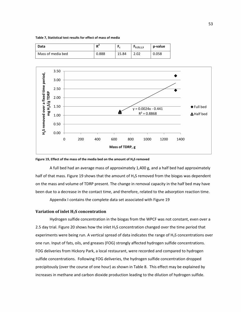
53
Table 7, Statistical test results for effect of mass of media
Data R2 Fc F0.25,1,3 p-value
Mass of media bed 0.888 15.84 2.02 0.058
Figure 19, Effect of the mass of the media bed on the amount of H2S removed
A full bed had an average mass of approximately 1,400 g, and a half bed had approximately
half of that mass. Figure 19 shows that the amount of H2S removed from the biogas was dependent
on the mass and volume of TDRP present. The change in removal capacity in the half bed may have
been due to a decrease in the contact time, and therefore, related to the adsorption reaction time.
Appendix I contains the complete data set associated with Figure 19
Variation of inlet H2S concentration
Hydrogen sulfide concentration in the biogas from the WPCF was not constant, even over a
2.5 day trial. Figure 20 shows how the inlet H2S concentration changed over the time period that
experiments were being run. A vertical spread of data indicates the range of H2S concentrations over
one run. Input of fats, oils, and greases (FOG) strongly affected hydrogen sulfide concentrations.
FOG deliveries from Hickory Park, a local restaurant, were recorded and compared to hydrogen
sulfide concentrations. Following FOG deliveries, the hydrogen sulfide concentration dropped
precipitously (over the course of one hour) as shown in Table 8. This effect may be explained by
increases in methane and carbon dioxide production leading to the dilution of hydrogen sulfide.
y = 0.0024x - 0.441
R² = 0.8868
0.00
0.50
1.00
1.50
2.00
2.50
3.00
3.50
0 200 400 600 800 1000 1200 1400
H2S
re
mo
ve
d o
ve
r a
fix
ed
tim
e p
eri
od
,
mg
H2S
/g T
DR
P
Mass of TDRP, g
Full bed
Half bed
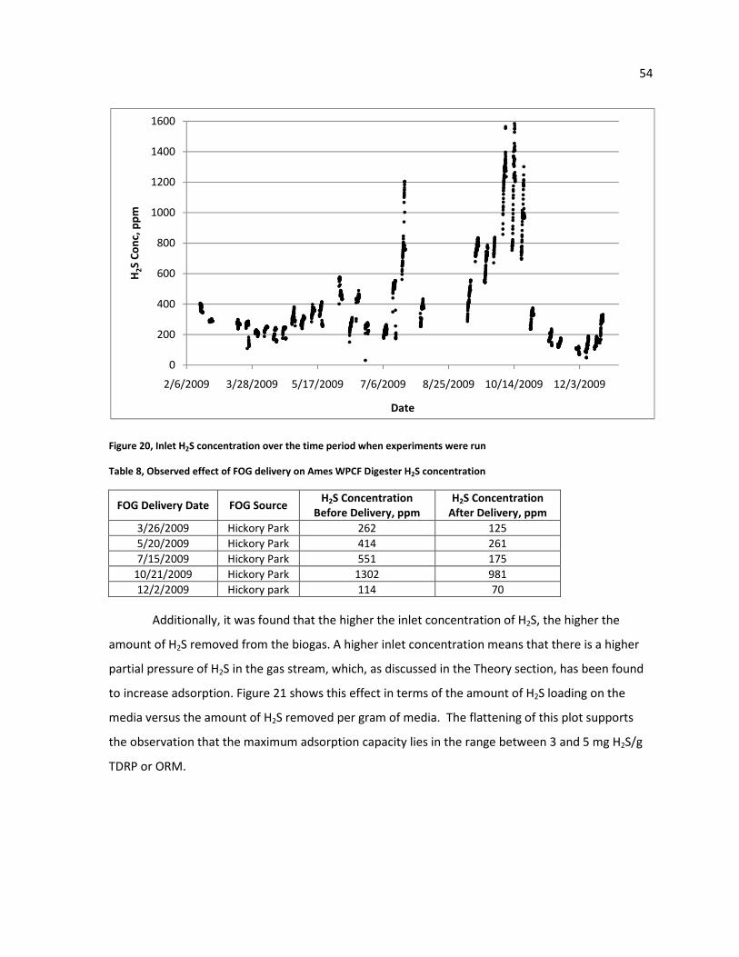
54
Figure 20, Inlet H2S concentration over the time period when experiments were run
Table 8, Observed effect of FOG delivery on Ames WPCF Digester H2S concentration
FOG Delivery Date FOG Source H2S Concentration
Before Delivery, ppm
H2S Concentration
After Delivery, ppm
3/26/2009 Hickory Park 262 125
5/20/2009 Hickory Park 414 261
7/15/2009 Hickory Park 551 175
10/21/2009 Hickory Park 1302 981
12/2/2009 Hickory park 114 70
Additionally, it was found that the higher the inlet concentration of H2S, the higher the
amount of H2S removed from the biogas. A higher inlet concentration means that there is a higher
partial pressure of H2S in the gas stream, which, as discussed in the Theory section, has been found
to increase adsorption. Figure 21 shows this effect in terms of the amount of H2S loading on the
media versus the amount of H2S removed per gram of media. The flattening of this plot supports
the observation that the maximum adsorption capacity lies in the range between 3 and 5 mg H2S/g
TDRP or ORM.
0
200
400
600
800
1000
1200
1400
1600
2/6/2009 3/28/2009 5/17/2009 7/6/2009 8/25/2009 10/14/2009 12/3/2009
H2S
Co
nc,
pp
m
Date

55
Figure 21, Relationship between H2S loading and specific H2S removal
Pressure Drop
The flow of biogas through the media bed caused a pressure drop across the bed. Figure 22
shows the pressure drop over the depth of the media bed versus the flow of biogas through the
system. As can be seen in Figure 22, it appears as if increasing the flow of biogas through the system
caused an increase in pressure drop over the depth of the media bed.
Figure 22, Pressure drop over the depth of the media bed (psi/ft) vs. flow of biogas through the system
0.00
1.00
2.00
3.00
4.00
5.00
6.00
0.0000 0.0500 0.1000 0.1500 0.2000 0.2500 0.3000 0.3500
H2S
re
mo
ve
d o
ve
r a
fix
ed
tim
e p
eri
od
, m
g
H2S
/g T
DR
P o
r O
RM
mg H2S/g TDRP or ORM/hr from inlet
Uncontrolled Half-Bed Constant Flow
Bed Compaction (~30%) Low Temp (20-30 F) High Temp (170 F)
Mid-Temp (75 F) ORM
y = -0.0018x2 + 0.0106x - 0.0063
R² = 0.2283
-0.005
0
0.005
0.01
0.015
0.02
0.025
0 0.5 1 1.5 2 2.5 3 3.5
Pre
ssu
re d
rop
ov
er
me
dia
de
pth
,
ΔP
/h,
psi
/ft
Flow, L/min

56
Comparison to other adsorbents
Hydrogen sulfide adsorption on other materials was tested in the scrubber system to serve
as a comparison to TDRP and ORM. Steel wool, a known H2S adsorbent, was tested in two trials. In
the trials using steel wool, breakthrough was immediate. After the first trial, the mass of steel wool
used was increased and the flow rate was decreased (so as to increase the empty bed contact time),
but breakthrough still occurred immediately. Therefore, under the environmental conditions
present in this study, TDRP and ORM were much better adsorbents of H2S.
Glass beads, which served as an inert surface, were also tested for one trial. Breakthrough
occurred immediately, although approximately one third of the way through the experiment the
beads began to show some capacity for H2S removal. This was thought to be due to water
condensation on the surface of the glass beads. Hydrogen sulfide can dissociate in water and is
therefore removed from the gas stream. This effect was also seen in other experiments where the
saturated media still appeared to be removing H2S from the biogas (as can be seen in the gap
between inlet and outlet H2S concentrations at the end of the experiment shown in Figure 10). To
remove the amount of H2S thought to be due solely to condensation in Figure 10, about 81 mL of
water condensation would be needed.
Data for these trials can be found in Appendix I.
Siloxane Testing
The effect of TDRP on siloxane (D4 and D5) removal was evaluated by sampling the biogas
before and after the scrubber (Table 9). For the first four tests, only inlet gas was sampled to
establish the background concentration, because only one sampling system was available. Based on
the results, the TDRP apparently removed in excess of 98% of the siloxanes from the biogas. ORM
was not tested for siloxane removal.

57
Table 9, Siloxane concentrations in biogas and outlet biogas from TDRP scrubber
Date Biogas Siloxane Concentration,
mg/m3
Scrubber Outlet Biogas Siloxane
Concentration mg/m3
4/25/2009 10.2 NTA
5/13/2009 1.12 NT
5/14/2009 0.72 NT
5/18/2009 3.59 NT
7/20/2009 75.6 1.32
8/4/2009 91.9 0.310
Average ± Standard Deviation 30.52 ± 41.69 0.815 ± 0.714 ANT = not tested
Isotherm Modeling
Freundlich Isotherm
Using Eq. 24, the Freundlich Isotherm can be fit to experimental data for ORM and TDRP.
Values for Ce and Xsat were taken from the raw data, converted to appropriate units, and plotted
using Eq. 24. The results can be seen in Figure 23 and Figure 24. The data used for Figure 23 and
Figure 24 were chosen because of the similar operating conditions in each trial. These operating
conditions included a biogas flow rate near 3 L/min, no compaction, a TDRP or ORM bed volume of
4,000 mL (therefore similar masses of TDRP or ORM), and temperature. “Isotherm” means the
temperature is held constant. In each of the trials used for the determination of Figure 23 and Figure
24, the temperature was relatively constant, around 25°C ± 3°C.
Figure 23, Freundlich Isotherm modeling of ORM at 25°C
y = 1.0982x + 0.1234
R² = 0.8451
-4.5
-4
-3.5
-3
-2.5
-2
-1.5
-1
-0.5
0
-4 -3.5 -3 -2.5 -2 -1.5 -1 -0.5 0
log
(Ce
, k
g H
2S
/m3)
log(Xsat, kg H2S/kg ORM)

58
Figure 24, Freundlich Isotherm modeling of TDRP at 25°C
The raw and converted data used in Figure 23 and Figure 24 can be found in Appendix I.
Using the slopes and y-intercepts of Figure 23 and Figure 24, α and β values for ORM and
TDRP were calculated. These results are shown in Table 10.
Table 10, Freundlich Isotherm constants at 25°C
α β
ORM 1.328 1.098
TDRP 0.020 0.542
The same method as described above was used to analyze the isotherms at other
temperatures. As described in the Materials and Methods section, the temperature control system
was set at 30°F/-1°C and 170°F/77°C for three experiments each on TDRP. These settings translated
to temperatures in the scrubber of 14-20°C and 44-52°C. Using data at these approximate
temperatures, isotherms for “low” and “high” temperatures were created and the Freundlich
Isotherm models for TDRP can be seen in Figure 25 and Figure 26. Data used for both of these
figures can be found in Appendix I.
y = 0.5418x - 1.7009
R² = 0.8141
-4.00
-3.50
-3.00
-2.50
-2.00
-1.50
-1.00
-0.50
0.00
-4 -3.5 -3 -2.5 -2 -1.5 -1 -0.5 0
log
(Ce
, k
g H
2S
/m3)
log(Xsat, kg H2S/kg TDRP)

59
Figure 25, Freundlich Isotherm modeling for TDRP at 14-20°C (low temperatures)
Figure 26, Freundlich Isotherm modeling for TDRP at 44-52°C (high temperatures)
Figure 25 for low temperature shows a satisfactory correlation of the Freundlich model to
the data. However, Figure 26 for high temperature shows a very poor correlation of the model to
the data. Unfortunately, due to time constraints, additional data for high temperature was not able
y = -0.1901x - 3.6742
R² = 0.8309
-3.50
-3.00
-2.50
-2.00
-1.50
-1.00
-0.50
0.00
-4.50 -4.00 -3.50 -3.00 -2.50 -2.00 -1.50 -1.00 -0.50 0.00lo
g (
Ce
, k
g H
2S
/m3)
log (Xsat, kg H2S/kg TDRP)
y = -0.0265x - 3.4037
R² = 0.0009
-4.00
-3.50
-3.00
-2.50
-2.00
-1.50
-1.00
-0.50
0.00
-3.50 -3.00 -2.50 -2.00 -1.50 -1.00 -0.50 0.00
log
(C
e,
kg
H2S
/m3)
log (Xsat, kg H2S/kg TDRP)

60
to be collected. The α and β Freundlich constants were calculated for low temperature, but not at
high temperature, due to the lack of correlation of the model to the data. The constants for low
temperature are shown in Table 11.
Table 11, Freundlich Isotherm constants for TDRP at 14-20°C (low temperature)
Langmuir Isotherm
The Langmuir Isotherm was also used to model the data. While the Freundlich Isotherm is
common for modeling experimental data due to its log-log determination of constants, the Langmuir
Isotherm does not model the data as easily. However, if the Langmuir Isotherm is a good fit to the
experimental data, then there is further evidence that the H2S adsorption occurs in a monolayer
over the media. The data was modeled according to the Langmuir Isotherm described by Eq. 16. The
isotherms for ORM and TDRP at 25°C can be seen in Figure 27 and Figure 28.
Figure 27, Langmuir Isotherm modeling of ORM at 25°C
y = 239.21x + 549.47
R² = 0.1757
0.00
200.00
400.00
600.00
800.00
1000.00
1200.00
0.00 0.20 0.40 0.60 0.80 1.00 1.20
Cg/W
Cg, g H2S/m3
α β
TDRP 2.117E-4 -0.190
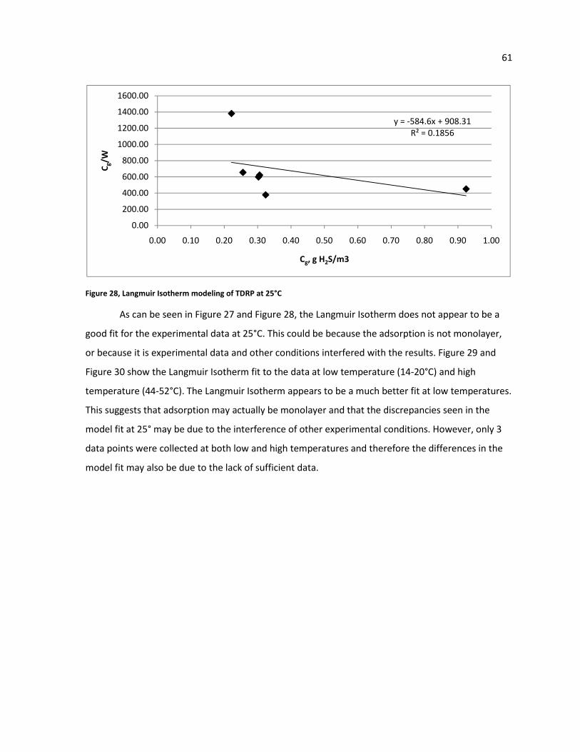
61
Figure 28, Langmuir Isotherm modeling of TDRP at 25°C
As can be seen in Figure 27 and Figure 28, the Langmuir Isotherm does not appear to be a
good fit for the experimental data at 25°C. This could be because the adsorption is not monolayer,
or because it is experimental data and other conditions interfered with the results. Figure 29 and
Figure 30 show the Langmuir Isotherm fit to the data at low temperature (14-20°C) and high
temperature (44-52°C). The Langmuir Isotherm appears to be a much better fit at low temperatures.
This suggests that adsorption may actually be monolayer and that the discrepancies seen in the
model fit at 25° may be due to the interference of other experimental conditions. However, only 3
data points were collected at both low and high temperatures and therefore the differences in the
model fit may also be due to the lack of sufficient data.
y = -584.6x + 908.31
R² = 0.1856
0.00
200.00
400.00
600.00
800.00
1000.00
1200.00
1400.00
1600.00
0.00 0.10 0.20 0.30 0.40 0.50 0.60 0.70 0.80 0.90 1.00
Cg/W
Cg, g H2S/m3

62
Figure 29, Langmuir Isotherm modeling of TDRP at 14-20°C (low temperature)
Figure 30, Langmuir Isotherm modeling of TDRP at 44-52°C (high temperature)
B.E.T. Isotherm
As described in the Theory section, the B.E.T. Model is used to model adsorption when there
are multiple layers of adsorbate molecules on the adsorbent surface. The B.E.T. Model is described
in Eq. 17. However, as also described in that section, the B.E.T. Model is difficult to evaluate when
the ratio of the partial pressure of the adsorbate in the gas stream to the vapor pressure of the
adsorbate at the system temperature is less than 0.05. This ratio was calculated to be approximately
8.5 x 10⁻³ for the highest concentration measured over the course of this study, 1600 ppm.
Therefore, it was not attempted to fit this model to the experimental data.
y = 17790x - 12372
R² = 0.9989
0.00
2000.00
4000.00
6000.00
8000.00
10000.00
12000.00
0.00 0.20 0.40 0.60 0.80 1.00 1.20 1.40
Cg/W
Cg, g/m3
y = 1171x - 181.02
R² = 0.6106
0.00
100.00
200.00
300.00
400.00
500.00
600.00
700.00
800.00
900.00
0.00 0.10 0.20 0.30 0.40 0.50 0.60 0.70 0.80
Cg/W
Cg, g/m3
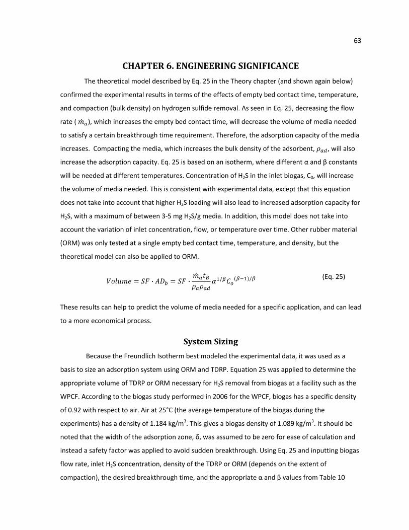
63
CHAPTER 6. ENGINEERING SIGNIFICANCE
The theoretical model described by Eq. 25 in the Theory chapter (and shown again below)
confirmed the experimental results in terms of the effects of empty bed contact time, temperature,
and compaction (bulk density) on hydrogen sulfide removal. As seen in Eq. 25, decreasing the flow
rate ( �3 /), which increases the empty bed contact time, will decrease the volume of media needed
to satisfy a certain breakthrough time requirement. Therefore, the adsorption capacity of the media
increases. Compacting the media, which increases the bulk density of the adsorbent, 4/2, will also
increase the adsorption capacity. Eq. 25 is based on an isotherm, where different α and β constants
will be needed at different temperatures. Concentration of H2S in the inlet biogas, C0, will increase
the volume of media needed. This is consistent with experimental data, except that this equation
does not take into account that higher H2S loading will also lead to increased adsorption capacity for
H2S, with a maximum of between 3-5 mg H2S/g media. In addition, this model does not take into
account the variation of inlet concentration, flow, or temperature over time. Other rubber material
(ORM) was only tested at a single empty bed contact time, temperature, and density, but the
theoretical model can also be applied to ORM.
���K�� � �� · FG � �� · �3 /DE4/4/2 ,5/1�7�185�/1 (Eq. 25)
These results can help to predict the volume of media needed for a specific application, and can lead
to a more economical process.
System Sizing
Because the Freundlich Isotherm best modeled the experimental data, it was used as a
basis to size an adsorption system using ORM and TDRP. Equation 25 was applied to determine the
appropriate volume of TDRP or ORM necessary for H2S removal from biogas at a facility such as the
WPCF. According to the biogas study performed in 2006 for the WPCF, biogas has a specific density
of 0.92 with respect to air. Air at 25°C (the average temperature of the biogas during the
experiments) has a density of 1.184 kg/m3. This gives a biogas density of 1.089 kg/m3. It should be
noted that the width of the adsorption zone, δ, was assumed to be zero for ease of calculation and
instead a safety factor was applied to avoid sudden breakthrough. Using Eq. 25 and inputting biogas
flow rate, inlet H2S concentration, density of the TDRP or ORM (depends on the extent of
compaction), the desired breakthrough time, and the appropriate α and β values from Table 10

64
produced Eq. 27, which gives the necessary volume of TDRP that will be required when the gas is
25°C.
���K�� �FQ& �R SQT � �� · �GDE10004/2 , 51�1.39�10U ��185�/1 (Eq. 27)
In Eq. 27, Vb is the biogas flow rate in L/min, C is inlet concentration of H2S in ppm, tB is the desired
breakthrough time of the system in minutes, and ρad is the density of the TDRP in kg/m3. The volume
of TDRP required is in m3.
From the Ames WPCF Digester Gas Improvements Study, it was estimated that the
anaerobic digesters produce about 56,800 ft3 of biogas per year. To estimate the size of an H2S
removal system needed at the WPCF using TDRP or ORM, a few assumptions were made when using
Eq. 7. If the biogas production is averaged evenly over a course of a year, a flow of 3.06 L/min of
biogas comes from the digesters. From looking at Figure 20 it seems as if the inlet concentration of
H2S was most often around 300 ppm. The density of ORM was taken to be 250 kg/m3 and TDRP was
375 kg/m3, which are approximately in the middle of the ranges of TDRP/ORM densities. If the
desired breakthrough time was one year, then the approximate volume of ORM and TDRP needed
would be 4.16 m3 and 2.26 m3, respectively. Inlet H2S concentration, biogas flow, and temperature
may be variable in actual system conditions, and therefore a safety factor should be used in order to
prevent premature breakthrough. If a safety factor of 3 is used, then approximately 12.48 m3 of
ORM or 6.77 m3 of TDRP would be needed on a yearly basis. Dimensions of the scrubber system
could be chosen to fit the necessary volume.
The volume of TDRP required would be different if a different temperature in the scrubber is
maintained. The concentration conversion from ppm to kg/m3 would change to 1.43E-6 at low
temperature (average temperature is 17°C) from 1.39E-6 at 25°C. Using the Freundlich constants
from Table 11, an assumed flow rate of 3.06 L/min of biogas, an inlet H2S concentration of 300ppm,
and a TDRP density of 375 kg/m3, the volume of TDRP necessary for one year of H2S adsorption at
the WPCF is 0.08 m3. When a safety factor of 3 is used, then approximately 0.23 m3 of TDRP would
be needed. Economically, the smaller amount of media needed at a lower temperature must be
balanced against the cost of cooling the gas to a lower temperature.

65
The validity of this model can be checked by using Eq. 25 to predict the volume of media
needed under certain conditions and then comparing the predicted volume with the actual volume
used. For TDRP using the Freundlich Isotherm, Table 12 is the volume of TDRP used in the
experiment compared to the predicted volume of TDRP needed for breakthrough to occur under the
operational conditions in each trial, which is found by imputing mass flow rate, bulk density of TDRP,
average inlet concentration, and time until breakthrough occurred. No safety factor was added to
the calculation of predicted volume. Additionally, the width of the adsorption zone was assumed to
be zero, which could introduce some error into the calculation. The trials shown are the same trials
used to determine the Freundlich constants for TDRP at 25°C.
Table 12, Measured vs. predicted volume of TDRP needed using experimental data
Trial
Measured volume of
TDRP, mL Volume of bed, mL Predicted volume, mL % difference
7 4000 4291 4765 16
8 4000 4291 7233 45
9 4000 4291 5434 26
10 4000 4291 5177 23
23 4000 4355 2506 -60
34 4000 4436 3170 -26
Average 4000 4326 4714 4
The “Measured volume of TDRP” is the volume of TDRP that was measured using a beaker. The
“Volume of bed” is the calculated volume of the space the TDRP occupied in the scrubber, found
using the bed height and area of the scrubber cross-section. The “Predicted volume” describes the
volume calculated using Eq. 25 (without the safety factor) and other experimental parameters that
are listed in Appendix I.
Table 12 raises some interesting points. First, the measured volume of TDRP was always
4,000 mL because it was always measured in the same beaker, which had a capacity of 4,000 mL.
This volume of TDRP almost always filled the same bed volume, which was approximately 300 mL
more than was measured. The reason for the discrepancy is probably because the TDRP became
more separated as it was poured into the scrubber, causing it to take up more volume. Second, the
volume of TDRP predicted by the rest of the experimental parameters and results differed by up to
60%. This is most likely due to the assumptions made about the system to use Eq. 25 (width of
adsorption zone is zero and constant temperature, inlet concentration, and flow rate). This large

66
difference makes it difficult to accurately predict the volume of TDRP that will be actually needed,
and that is why adding a safety factor of at least 3 is necessary. However, when percent differences
in the last column are averaged over the six experiments, there is only a 4% average difference
between the predicted volume and the volume used.
The results found in this study were compared with results from another study about
different adsorbents. A study by Tsai, Jeng, & Chiang (2001) modeled the Freundlich Isotherm to
experimental H2S adsorption data of unimpregnated and impregnated activated carbons. Using the
Freundlich constants found by Tsai et al., an estimated activated carbon density of 560 kg/m3, and
the same conditions used in estimating TDRP and ORM volume (flow rate and H2S concentration),
Eq. 27 can be applied to estimate the volume of unimpregnated and impregnated activated carbon
needed. It was found that 1.92E-03 m3 of unimpregnated activated carbon and 1.66E-04 m3 of
activated carbon impregnated with NaOH would be needed to remove H2S at the WPCF for one
year. If a safety factor of 3 is applied, then 5.77E-3 m3 (5770 cm3) of unimpregnated and 4.97E-4 m3
(497 cm3) of impregnated activated carbon would be needed. This is a significantly less volume of
media than required for a TDRP or ORM scrubber.
A rough cost analysis can be performed to determine the minimum cost that TDRP or ORM
must have to compete with unimpregnated activated carbon. A quote from Calgon Corporation
(Pittsburgh, PA) for unimpregnated activated carbon was $8.44/lb. An information sheet for this
type of activated carbon lists the density as 560 kg/m3. Using the volume of unimpregnated
activated carbon calculated above, the cost per year of using unimpregnated activated carbon at the
WPCF would be about $60. This would mean that TDRP would have to cost $8.89/m3 ($0.024/kg)
and ORM would have to cost $4.82/m3 ($0.019/kg) to cost the same as activated carbon. This
assumes that the activated carbon is not regenerated. Impregnated activated carbon would cost
more than unimpregnated activated carbon, but a cost estimate was not available.
67
CHAPTER 7. CONCLUSION
Tire-derived rubber particles (TDRP) were tested at various conditions to determine optimal
operating conditions for the removal of hydrogen sulfide from biogas at the Ames WPCF.
A longer empty bed contact time increased the amount of H2S that was adsorbed up until
the time of breakthrough. However, over a standard period of time that always exceeded the
breakthrough time, it was seen that there was a maximum amount of H2S was adsorbed by the
media bed.
Compaction of the media bed resulted in improved H2S adsorption capacity per unit mass of
TDRP. It was hypothesized that this was due to reduced biogas short-circuiting in the scrubber.
Compaction of the media bed to approximately 65% of its original volume was tested and was found
to improve adsorption capacity by an average of 0.76 mg H2S/g TDRP.
Temperature was not found to have a significant effect on the amount of H2S that was
adsorbed. Ambient temperature, around 25°C, was the most common temperature tested, but
there were also tests at lower (14-20°C) and higher temperatures (44-52°C) that did not reveal a
significant difference in H2S adsorbed.
The concentration of H2S in the biogas varied greatly over the course of the year during
which the experiments were run and also during the course of individual trials. Large additions of
fat, oil, and grease (FOG) caused drastic drops in H2S concentration. It was found that the higher the
H2S loading from the inlet biogas on the media, the more H2S was adsorbed.
Preliminary testing of siloxane concentrations in the inlet and outlet biogas from the
scrubber showed that in excess of 98% of siloxanes could be removed using TDRP as the media.
Recommendations for Future Studies
The results of this study have shown that TDRP and ORM are viable materials that can be
used for H2S adsorption. However, there are still some pertinent issues that need to be addressed
before this product can be commercially used.
It is important that materials currently on the market for H2S adsorption (such as activated
carbon) have the ability to be regenerated, so as to make the process more economical. No

68
desorption experiments were performed during this study, so it is unknown if desorption is a
possibility using TDRP or ORM. If desorption and regeneration are possible, the economics of
performing this process should be compared to disposing of spent material and purchasing virgin
material. As the virgin material is derived from a waste product, it may be more economic to use
virgin material as opposed to regenerating the spent material.
Cost limitations during this study prevented any analysis of spent TDRP or ORM. Before this
product can be commercially implemented, it is important to determine the nature of the waste
being produced from the adsorption process. A Toxicity Characteristic Leaching Procedure (TCLP)
should be performed to determine if the spent material is a characteristic hazardous waste.
Additionally, it should be determined if the spent TDRP or ORM can be used in other applications,
such as an asphalt modifier or in molded products, as virgin crumb rubber is used.
Another interesting future study could determine the effects of other components in the
biogas on H2S adsorption. Biogas contains large portions of carbon dioxide and methane, and it is
possible that these compounds could interfere with adsorption onto the surface sites of the TDRP or
ORM. This study would also relate to determining the adsorption mechanism of H2S.
Perhaps the most promising results of this study relate to the ability of TDRP and ORM to
remove siloxanes from biogas. The results presented in this study about siloxanes pertain mostly to
some preliminary testing of siloxane concentrations in biogas. These results were extended by
another researcher over the course of this study. The results of the other study confirmed that both
TDRP and ORM can remove siloxanes from biogas by testing siloxane concentrations before and
after the scrubber. There did not appear to be a relationship between H2S and siloxane removal,
however only two trials were tested. Additional research could focus on conditions for maximizing
siloxane removal, as this study primarily focused on conditions for maximizing H2S removal.

69
REFERENCES
Abatzoglou, N. & Boivin, S. (2009). A review of biogas purification processes. Biofuels, Bioproducts
and Biorefining, 3, 42-71.
Adib, F., Bagreev, A., & Bandosz, T. J. (2000). Analysis of the relationship between H2S removal
capacity and surface properties of unimpregnated activated carbons. Environmental Science
and Technology, 24, 686-692.
Amari, T., Themelis, N.J., Wernick, I.K. (1999). Resource recovery from used rubber tires. Resources
Policy, 25, 179-188.
Arizona Instrument LLC. (2005). Jerome® 860 hydrogen sulfide monitor operation manual. Retrieved
December 15, 2009 from < http://www.azic.com/pdf/manual_700-0051.pdf>
American Society for Testing and Materials. (2003). Standard test method for determination of the
accelerated hydrogen sulfide breakthrough capacity of granular and pelletized activated
carbon.”Designation: D 6646-03.
Bandosz, T. J. (2002). On the adsorption/oxidation of hydrogen sulfide on activated carbons at
ambient temperatures. Journal of Colloid and Interface Science, 246, 1-20.
Bagreev, A. & Bandosz, T.J. (2002). A role of sodium hydroxide in the process of hydrogen sulfide
adsorption/oxidation on caustic-impregnated activated carbons. Industrial & Engineering
Chemical Research, 41, 672-679.
Bagreev, A., Katikaneni, S., Parab, S., & Bandosz, T.J. (2005). Desulfurization of digester gas:
prediction of activated carbon bed performance at low concentrations of hydrogen sulfide.
Catalysis Today, 99, 329-337.
Carnes, C. L. & Klabunde, K. J. (2002). Unique chemical reactivities of nanocrystalline metal oxides
toward hydrogen sulfide. Chemistry of Materials, 14, 1806-1811.
Davidson, J. M., Lawrie, C. H., & Sohail, K. (1995). Kinetics of the absorption of hydrogen sulfide by
high purity and doped surface area zinc oxide. Industrial and Engineering Chemistry
Research, 34, 2981-2989.
Davis, M. & Cornwell, D. (2008). Introduction to environmental engineering. Boston, MA: McGraw-
Hill.
Ellis, T. (2005). Evaluation of tire rubber particles (TDRP) for biofiltration media. Draft final report for
Envirotech Systems, Inc.
Ellis, T., Park, J., & Oh, J. (2008). A novel and cost-effective H2S absorption technology using tire
derived rubber particles. Submitted to IPRT Company Assistance: Grow Iowa Values Fund
Seed Grant.

70
Hedden, K., Humber, L. & Rao, B.R. (1976).VDI-Bericht 253 S. 37/42. VDI-Verlag, Duesseldorf.
Keller, J. & Staudt, R. (2005). Gas adsorption equilibria: Experimental methods and adsorption
isotherms. New York, NY: Springer Science and Business Media, Inc.
Kohl, A. & Nielsen, R. (1997). Gas Purification. Houston, TX: Gulf Publishing Company.
Lee, J.D., Jun, J.H., Park, N.; Ryu, S., & Lee, T. J. (2005). A study on selective oxidation of hydrogen
sulfide over zeolite-NaX and-KX catalysts. Korean Journal of Chemical Engineering, 22, 36-41.
McBean, E. (2008). Silxanes in biogases from landfills and wastewater digesters. Canadian Journal of
Civil Engineering, 35, 4, 431-436.
McCrady, E. (1996). Zeolites. Conservation OnLine: Abbey Newsletter. 20 (7), Dec. 1996.
<http://palimpsest.stanford.edu/byorg/abbey/an/an20/an20-7/an20-702.html>
McKinsey Zicarai, S. (2003). Removal of hydrogen sulfide from biogas using cow-manure compost.
Thesis Presented to the Faculty of the Graduate School of Cornell University, 1-104.
Nagl, G. (1997). Controlling H2S emissions. Chemical Engineering, 104(3), 125-131.
Osorio, F. & Torres, J.C. (2009). Biogas purification from anaerobic digestion in a wastewater
treatment plant for biofuel production. Renewable Energy, 34, 2164-2171.
Rodriguez, J.A. & Maiti, A. (2000). Adsorption and decomposition of H2S on MgO(100), NiMgO(100),
and ZnO(0001) surfaces: A first-principles density functional study. Journal of Physical
Chemistry B, 104, 3630-3638.
Saeed, S., Kao, S., & Graening, G. (2002). Comparison of impinge and canister methods for the
determination of siloxanes in air. Presented at the AWMA Symposium on Air Quality
Measurement methods and Technology in San Francisco, CA. Retrieved January 15, 2010
from < http://www.airtoxics.com/literature/papers/Siloxanes_Paper_AWMA.pdf>
Sunthonpagasit, N. & Duffey, M.R. (2004). Scrap tires to crumb rubber: Feasibility Analysis for
Processing Facilities. Resources Conservation & Recycling,40, 281-299.
Trapezoidal Rule. (2010). In Wikipedia, the free encyclopedia. Retrieved February 1, 2010 from
<http://en.wikipedia.org/wiki/Trapezoidal_rule>
Truong, L.V.-A. & Abatzoglou, N. (2005). A H2S reactive adsorption process for the purification of
biogas prior to its use as a bioenergy vector. Biomass and Bioenergy, 29, 142-151.
Tsai, J., Jeng, F., Chiang, H. (2001). Removal of H2S from exhaust gas by use of alkaline activated
carbon. Adsorption, 7, 357-366.

71
U.S. Environmental Protection Agency. (2009). Ground Rubber Applications. Retrieved November
23, 2009 from <http://www.epa.gov/osw/conserve/materials/tires/ground.htm>
U.S. Environmental Protection Agency. (2003). Toxicological Review of Hydrogen Sulfide (CAS No.
7783-06-4). Retrieved September 23, 2009 from
<http://www.epa.gov/ncea/iris/toxreviews/0061-tr.pdf>
Wang, X., Ma, X., Xu, X., Sun, L., & Song, C. (2008). Mesoporous-molecular-sieve-supported polymer
sorbents for removing H2S from hydrogen gas streams. Topics in Catalysis, 49, 108-117.
Wark, K., Warner, C., & Davis, W. (1998). Air pollution: Its origin and control. Menlo Park, CA:
Addison Wesley Longman.
Wheeler, P., Jaatinen, T., Lindberg, A., Holm-Nielsen, J.B., Wellinger, A., & Pettigrew, A. (2000).
Biogas Upgrading and Utilisation. IEA Bioenergy Task 24. International Energy Association,
Paris, France.
Yan, R., Chin, T., Ng, Y.L., Duan, H., Liang, D.T., & Tay, J.H. (2004). Influence of surface properties on
the mechanism of H2S removal by alkaline activated carbons. Environmental Science &
Technology, 38, 316-323.
Yuan, W. & Bandosz, T.J. (2007). Removal of hydrogen sulfide from biogas on sludge-derived
adsorbents. Fuel, 86, 2736-2746.
Xiao, Y., Wang, S., Wu, D., & Yuan, Q. (2008). Experimental and simulation study of hydrogen sulfide
adsorption on impregnated activated carbon under anaerobic conditions. Journal of
Hazardous Materials, 153, 1193-1200.

72
APPENDIX I: HYDROGEN SULFIDE TESTING RESULTS
Empty Bed Contact Time
Table 13 lists the complete data for each trial used to evaluate the effect of empty bed
contact time on H2S adsorption by TDRP.
Table 13, Raw data for empty bed contact time effects
Trial 7 Trial 8 Trial 9 Trial 10 Trial 26
Trial
27
Mass of TDRP, g 1420 1500 1420 1500 1580 1580
Vol of TDRP, mL 4000 4000 4000 4000 4000 4000
Avg Flow Rate, L/min 3.13 2.09 3.13 3.13 1.04 0.52
Total Adsorbed, mg H2S/g TDRP 1.19 1.29 1.09 1.13 1.09 1.10
Adsorbed at breakthrough, mg
H2S/g TDRP 0.49 0.86 0.39 0.51 0.67 1.09
Time until breakthrough, min 794 2002 779 903 2046 3524
Empty bed contact time, s 81.48 134.57 83.23 83.23 256.42 483.30
H2S Sensor inlet temp, C 28.4 24 24.7 28.3 22.7 23.1
H2S Sensor outlet temp, C 28.4 24 24.7 28.1 22.8 23.1
Temp avg, C (temp probe in
scrubber) 28.8 25.5 25.4 28.7 23.1 24.0
Temp stdev, C (temp probe in
scrubber) 1.4 3.7 2.8 2.3 6.5 1.8
Temp Dial Avg, C 27.1 24
mg H2S/g TDRP/hr from inlet 0.0390 0.0281 0.0377 0.0389 0.0246 0.0216
Average outlet H2S conc before
breakthrough 9.0 12.1 6.9 7.8 28.9 100.9
Stdev outlet H2S conc before
breakthrough 5.6 4.8 2.2 3.7 11.3 29.7
Average inlet H2S conc before
breakthrough 220.0 233.1 184.1 217.6 390.9 772.3
Stdev inlet H2S conc before
breakthrough 6.0 11.6 11.2 21.0 43.1 38.8
Temperature
Table 14 lists the complete data for each trial used to evaluate the effect of low
temperature on H2S adsorption by TDRP. It should be noted that for Trials 22 and 30, the data
logging thermocouple was malfunctioning so a dial thermometer was installed in the scrubber and
manual readings were taken four times over the course of the trial and averaged.

73
Table 14, Raw data for low temperature effect
Trial 16 Trial 22 Trial 30
Mass of TDRP, g 1161 1420 1640
Vol of TDRP, mL 4000 4000 4000
Avg Flow Rate, L/min 2.6 3.13 3.13
Total Adsorbed, mg H2S/g TDRP 3.01 3.51 3.66
Adsorbed at breakthrough, mg H2S/g TDRP 0.56 2.31 0.13
Time until breakthrough, min 401 1621 124
Empty bed contact time, s 96.70 81.12 83.37
H2S Sensor inlet temp, C 33.2 25.2 16.0
H2S Sensor outlet temp, C 33.2 25.2 16.0
Temp avg, C (temp probe in scrubber) 16.9
Temp stdev, C (temp probe in scrubber) 5.6 13.7 8.9
Temp Dial Avg, C 20.7 14.2
mg H2S/g TDRP/hr from inlet 0.0905 0.0850 0.2021
Average outlet H2S conc before breakthrough 33.8 24.77 58.04
Stdev outlet H2S conc before breakthrough 8.5 5.69 17.10
Average inlet H2S conc before breakthrough 533.2 505.16 874.87
Stdev inlet H2S conc before breakthrough 60.8 39.36 24.47
Table 15 lists the complete data for each trial used to evaluate the effect of medium
temperature on H2S adsorption by TDRP. It should be noted that for Trial 23 the data logging
thermocouple was malfunctioning and the temperature used was taken from the dial thermometer
in the scrubber.

74
Table 15, Raw data for medium temperature effect
Trial 7 Trial 8 Trial 9 Trial 10 Trial 23 Trial 26 Trial 27 Trial 34
Mass of TDRP, g 1420 1500 1420 1500 1380 1580 1580 1620
Vol of TDRP, mL 4000 4000 4000 4000 4000 4000 4000 4000
Avg Flow Rate, L/min 3.1 2.1 3.1 3.1 3.13 1.04 0.52 3.13
Total Adsorbed, mg H2S/g TDRP 1.19 1.29 1.09 1.13 5.19 1.09 1.10 0.49
Adsorbed at breakthrough, mg H2S/g TDRP 0.49 0.86 0.39 0.51 2.05 0.67 1.09 0.16
Time until breakthrough, min 794 2002 779 903 1034 2046 3524 459
Empty bed contact time, s 81.48 134.57 83.23 83.23 81.85 256.42 483.3 83.37
H2S Sensor inlet temp, C 28.4 24 24.7 28.3 22.82 22.70 23.09 24.18
H2S Sensor outlet temp, C 28.4 24 24.7 28.1 22.82 22.76 23.11 24.20
Temp avg, C (temp probe in scrubber) 28.8 25.5 25.4 28.7 23.05 23.98 25.19
Temp stdev, C (temp probe in scrubber) 1.4 3.7 2.8 2.3 9.4 6.50 1.81 1.09
Temp Dial Avg, C 26.4 27.1 24 27.5
mg H2S/g TDRP/hr from inlet 0.0390 0.0281 0.0377 0.0389 0.2180 0.0246 0.0216 0.0296
Average outlet H2S conc before breakthrough 9.0 12.1 6.9 7.8 34.00 28.93 100.86 19.05
Stdev outlet H2S conc before breakthrough 5.6 4.8 2.2 3.7 6.70 11.26 29.66 2.13
Average inlet H2S conc before breakthrough 220.0 233.1 184.1 217.6 664.97 390.95 772.27 159.46
Stdev inlet H2S conc before breakthrough 6.0 11.6 11.2 21.0 46.13 43.12 38.77 2.77
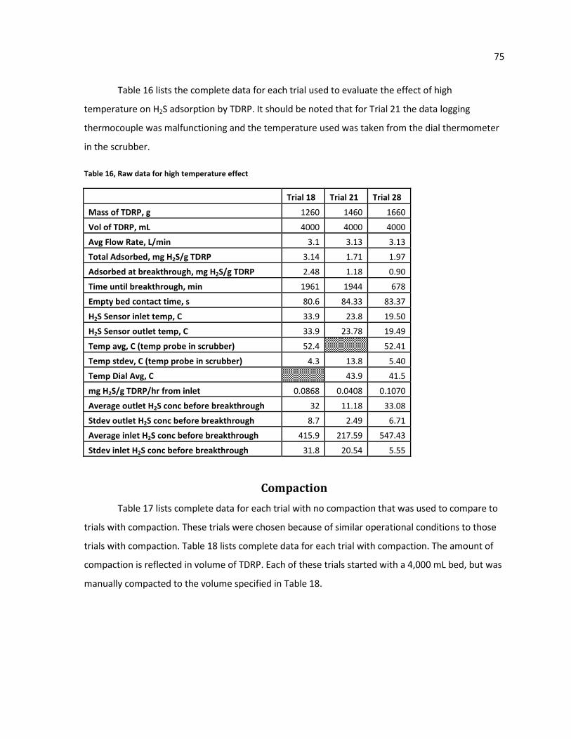
75
Table 16 lists the complete data for each trial used to evaluate the effect of high
temperature on H2S adsorption by TDRP. It should be noted that for Trial 21 the data logging
thermocouple was malfunctioning and the temperature used was taken from the dial thermometer
in the scrubber.
Table 16, Raw data for high temperature effect
Trial 18 Trial 21 Trial 28
Mass of TDRP, g 1260 1460 1660
Vol of TDRP, mL 4000 4000 4000
Avg Flow Rate, L/min 3.1 3.13 3.13
Total Adsorbed, mg H2S/g TDRP 3.14 1.71 1.97
Adsorbed at breakthrough, mg H2S/g TDRP 2.48 1.18 0.90
Time until breakthrough, min 1961 1944 678
Empty bed contact time, s 80.6 84.33 83.37
H2S Sensor inlet temp, C 33.9 23.8 19.50
H2S Sensor outlet temp, C 33.9 23.78 19.49
Temp avg, C (temp probe in scrubber) 52.4 52.41
Temp stdev, C (temp probe in scrubber) 4.3 13.8 5.40
Temp Dial Avg, C 43.9 41.5
mg H2S/g TDRP/hr from inlet 0.0868 0.0408 0.1070
Average outlet H2S conc before breakthrough 32 11.18 33.08
Stdev outlet H2S conc before breakthrough 8.7 2.49 6.71
Average inlet H2S conc before breakthrough 415.9 217.59 547.43
Stdev inlet H2S conc before breakthrough 31.8 20.54 5.55
Compaction
Table 17 lists complete data for each trial with no compaction that was used to compare to
trials with compaction. These trials were chosen because of similar operational conditions to those
trials with compaction. Table 18 lists complete data for each trial with compaction. The amount of
compaction is reflected in volume of TDRP. Each of these trials started with a 4,000 mL bed, but was
manually compacted to the volume specified in Table 18.

76
Table 17, Raw data for trials with no compaction
Trial 7 Trial 9 Trial 10
Mass of TDRP, g 1420 1420 1500
Vol of TDRP, mL 4000 4000 4000
Avg Flow Rate, L/min 3.1 3.1 3.1
Total Adsorbed, mg H2S/g TDRP 1.19 1.09 1.13
Adsorbed at breakthrough, mg H2S/g TDRP 0.49 0.39 0.51
Time until breakthrough, min 794 779 903
Empty bed contact time, s 81.48 83.23 83.23
H2S Sensor inlet temp, C 28.4 24.7 28.3
H2S Sensor outlet temp, C 28.4 24.7 28.1
Temp avg, C (temp probe in scrubber) 28.8 25.4 28.7
Temp stdev, C (temp probe in scrubber) 1.4 2.8 2.3
Temp Dial Avg, C
mg H2S/g TDRP/hr from inlet 0.0390 0.0377 0.0389
Average outlet H2S conc before breakthrough 9.0 6.9 7.8
Stdev outlet H2S conc before breakthrough 5.6 2.2 3.7
Average inlet H2S conc before breakthrough 220.0 184.1 217.6
Stdev inlet H2S conc before breakthrough 6.0 11.2 21.0
Table 18, Raw data for trials with compaction
Trial 11 Trial 12 Trial 13 Trial 14
Mass of TDRP, g 1580 1440 1462 1378
Vol of TDRP, mL 2600 2680 2880 2640
Avg Flow Rate, L/min 3.1 3.1 3.5 2.6
Total Adsorbed, mg H2S/g TDRP 1.49 1.61 1.98 2.49
Adsorbed at breakthrough, mg H2S/g TDRP 0.77 0.62 0.87 1.74
Time until breakthrough, min 1001 807 909 2099
Empty bed contact time, s 60 56.13 53.14 65.77
H2S Sensor inlet temp, C 24.9 27 27.6 28.1
H2S Sensor outlet temp, C 24.9 27.1 27.6 28.1
Temp avg, C (temp probe in scrubber) 25.3 26.0 26.3
Temp stdev, C (temp probe in scrubber) 1.6 3.5 4.7
Temp Dial Avg, C
mg H2S/g TDRP/hr from inlet 0.0527 0.0520 0.0697 0.0533
Average outlet H2S conc before breakthrough 14.6 15.8 14.6 23.1
Stdev outlet H2S conc before breakthrough 6.8 2.1 6.1 5.8
Average inlet H2S conc before breakthrough 300.0 273.6 327.6 352.3
Stdev inlet H2S conc before breakthrough 13.6 8.5 16.9 21.4

77
Mass of Media Bed
The effect of the mass of the media bed on H2S adsorption by TDRP was determined by
comparing a full bed, defined as 4,000 mL, to a half bed, defined as 2,000 mL. Table 19 lists
complete data for the full bed trials that were compared to the half bed trials listed in Table 20. The
trials in Table 19 were selected out of all the trials that used a full bed because they had the most
similar operational conditions to the half bed trials in Table 20.
Table 19, Raw data for full bed TDRP mass
Trial 1 Trial 2
Mass of TDRP, g 1340 1340
Vol of TDRP, mL 4000 4000
Avg Flow Rate, L/min 5 4.9
Total Adsorbed, mg H2S/g TDRP 3.24 2.42
Adsorbed at breakthrough, mg H2S/g TDRP 2.72 1.69
Time until breakthrough, min 1465 1269
Empty bed contact time, s 50.52 51.55
H2S Sensor inlet temp, C 27.6 27.5
H2S Sensor outlet temp, C 27.4 27.4
Temp avg, C (temp probe in scrubber) 26.9 27.3
Temp stdev, C (temp probe in scrubber) 1.8 1.9
Temp Dial Avg, C
mg H2S/g TDRP/hr from inlet 0.1090 0.0860
Average outlet H2S conc before breakthrough 136.0 4.6
Stdev outlet H2S conc before breakthrough 14.8 10.7
Average inlet H2S conc before breakthrough 370.9 289.1
Stdev inlet H2S conc before breakthrough 18.7 3.7

78
Table 20, Raw data for half bed TDRP mass
Trial 5 Trial 6
Mass of TDRP, g 670 670
Vol of TDRP, mL 2000 2000
Avg Flow Rate, L/min 5.1 5.2
Total Adsorbed, mg H2S/g TDRP 1.17 1.22
Adsorbed at breakthrough, mg H2S/g TDRP 0.14 0.28
Time until breakthrough, min 100 136
Empty bed contact time, s 24.71 24.23
H2S Sensor inlet temp, C 26.9 26.1
H2S Sensor outlet temp, C 27 26.1
Temp avg, C (temp probe in scrubber) 26.4 26.6
Temp stdev, C (temp probe in scrubber) 3.7 7.2
Temp Dial Avg, C
mg H2S/g TDRP/hr from inlet 0.1714 0.1550
Average outlet H2S conc before breakthrough 46.7 33.3
Stdev outlet H2S conc before breakthrough 49.7 34.5
Average inlet H2S conc before breakthrough 274.3 248.9
Stdev inlet H2S conc before breakthrough 6.5 7.2
Comparison to Other Adsorbents
Steel wool and glass beads were used in the scrubber system to serve as a comparison to
TDRP and ORM. The results can be seen in Table 21.

79
Table 21, Raw data for trials with steel wool and glass beads
Trial 37 Trial 38 Trial 39
Mass of TDRP, g 120 280 6640
Vol of TDRP, mL 4000 4000 4000
Avg Flow Rate, L/min 2.6 1.0 1.0
Total Adsorbed, mg H2S/g TDRP 0.71 0.17 0.07
Adsorbed at breakthrough, mg H2S/g TDRP
Time until breakthrough, min
Empty bed contact time, s 96.53 244.5 253.16
H2S Sensor inlet temp, C 14.0 11.7 15.4
H2S Sensor outlet temp, C 14.0 11.7 15.3
Temp avg, C (temp probe in scrubber) 14.3 21.3 15.3
Temp stdev, C (temp probe in scrubber) 7.3 1.8 3.6
Temp Dial Avg, C 20.8 21.5 22.2
mg H2S/g TDRP/hr from inlet 0.2351 0.0485 0.0035
Average outlet H2S conc before breakthrough
Stdev outlet H2S conc before breakthrough
Average inlet H2S conc before breakthrough
Stdev inlet H2S conc before breakthrough
Material Steel wool Steel wool Glass beads
Isotherm Modeling
Experimental data was fit to the Freundlich Isotherm model. Measured and converted
values are shown in Table 22 and Table 23 for use in the Freundlich Isotherm for ORM and TDRP at
25°C. Data used for finding the “low temperature” isotherm for TDRP at 14-20°C and the “high
temperature” isotherm for TDRP at 44-52°C can be found in Table 24 and Table 25, respectively.
Table 26 through Table 29 show values used to model the Langmuir Isotherm.

80
Table 22, Raw and converted data used to find Freundlich constants for ORM at 25°C
Trial
Avg Inlet H2S Conc,
ppm
Adsorbed at breakthrough,
mg H2S/g TDRP Temp, C Ce, kg H2S/m3 Xsat, kg H2S/kg TDRP log(Ce) log(Xsat)
31 785.25 1.95 24.66 1.09E-03 1.95E-03 -2.96 -2.71
32 722.97 1.00 28.86 1.00E-03 9.98E-04 -3.00 -3.00
33 240.99 0.36 25.64 3.35E-04 3.64E-04 -3.47 -3.44
35 122.37 0.38 24.77 1.70E-04 3.79E-04 -3.77 -3.42
36 108.73 0.32 24.20 1.51E-04 3.22E-04 -3.82 -3.49
Table 23, Raw and converted data used to find Freundlich constants for TDRP at 25°C
Trial
Avg Inlet H2S Conc,
ppm
Adsorbed at breakthrough,
mg H2S/g TDRP Temp, C Ce, kg H2S/m3 Xsat, kg H2S/kg TDRP log(Ce) log(Xsat)
7 219.99 0.49 28.77 3.06E-04 4.92E-04 -3.51 -3.31
8 233.07 0.86 25.50 3.24E-04 8.57E-04 -3.49 -3.07
9 184.13 0.39 25.36 2.56E-04 3.91E-04 -3.59 -3.41
10 217.61 0.51 28.68 3.02E-04 5.05E-04 -3.52 -3.30
23 664.97 2.05 26.40 9.24E-04 2.05E-03 -3.03 -2.69
34 159.46 0.16 25.19 2.22E-04 1.60E-04 -3.65 -3.79
Table 24, Raw and converted data used to find Freundlich constants for TDRP at 14-20°C (low temperature)
Trial
Avg Inlet H2S Conc,
ppm
Adsorbed at breakthrough,
mg H2S/g TDRP Temp, C Ce, kg H2S/m3 Xsat, kg H2S/kg TDRP log(Ce) log(Xsat)
16 533.20 0.56 16.90 7.62E-04 5.56E-04 -3.12 -3.26
22 505.16 2.31 20.70 7.22E-04 2.31E-03 -3.14 -2.64
30 874.87 0.13 14.20 1.25E-03 1.27E-04 -2.90 -3.90

81
Table 25, Raw and converted data used to find Freundlich constants for TDRP at 44-52°C (high temperature)
Trial
Avg Inlet H2S Conc,
ppm
Adsorbed at breakthrough,
mg H2S/g TDRP Temp, C Ce, kg H2S/m3 Xsat, kg H2S/kg TDRP log(Ce) log(Xsat)
18 415.90 2.48 52.40 5.32E-04 2.48E-03 -3.27 -2.61
21 217.59 1.18 43.90 2.79E-04 1.18E-03 -3.56 -2.93
28 547.43 0.90 52.41 7.01E-04 9.02E-04 -3.15 -3.04
Table 26, Raw and converted data used to fit Langmuir Isotherm for ORM at 25°C
Trial
Avg Inlet
H2S Conc,
ppm Adsorbed at breakthrough, mg H2S/g TDRP Temp, C Cg, g/m3 W, kg H2S/kg TDRP Cg/W
31 785.25 1.95 24.66 1.09 1.95E-03 559.30
32 722.97 1.00 28.86 1.00 9.98E-04 1007.15
33 240.99 0.36 25.64 0.33 3.64E-04 920.30
35 122.37 0.38 24.77 0.17 3.79E-04 449.28
36 108.73 0.32 24.20 0.15 3.22E-04 469.79
Table 27, Raw and converted data used to fit Langmuir Isotherm for TDRP at 25°C
Trial
Avg Inlet
H2S Conc,
ppm Adsorbed at breakthrough, mg H2S/g TDRP Temp, C Cg, g/m3 W, kg H2S/kg TDRP Cg/W
7 219.99 0.49 28.77 0.31 4.92E-04 621.72
8 233.07 0.86 25.50 0.32 8.57E-04 378.12
9 184.13 0.39 25.36 0.26 3.91E-04 654.79
10 217.61 0.51 28.68 0.30 5.05E-04 598.44
23 664.97 2.05 26.40 0.92 2.05E-03 450.88
34 159.46 0.16 25.19 0.22 1.60E-04 1381.38

82
Table 28, Raw and converted data used to fit Langmuir Isotherm for TDRP at 14-20°C (low temperature)
Trial
Avg Inlet
H2S Conc,
ppm Adsorbed at breakthrough, mg H2S/g TDRP Temp, C Cg, g/m3 W, kg H2S/kg TDRP Cg/W
16 533.20 0.56 16.90 0.76 5.56E-04 1372.43
22 505.16 2.31 20.70 0.72 2.31E-03 312.72
30 874.87 0.13 14.20 1.25 1.27E-04 9870.72
Table 29, Raw and converted data used to fit Langmuir Isotherm for TDRP at 44-52°C (high temperature)
Trial
Avg Inlet
H2S Conc,
ppm Adsorbed at breakthrough, mg H2S/g TDRP Temp, C Cg, g/m3 W, kg H2S/kg TDRP Cg/W
18 415.90 2.48 52.40 0.53 2.48E-03 214.42
21 217.59 1.18 43.90 0.28 1.18E-03 236.03
28 547.43 0.90 52.41 0.70 9.02E-04 776.58
Table 30, Raw data to compare actual and predicted volumes of TDRP
Trial Ce, kg/m3
Volume,
mL ρad, kg/m^3
Mass flow rate,
kg/s Vad, m/s Db, m tB, min Predicted Volume, mL
7 3.06E-04 4000 8.36E-05 5.68E-05 1.07E-05 0.4207 794 4765
8 3.24E-04 4000 8.86E-05 3.79E-05 6.42E-06 0.4207 2002 7233
9 2.56E-04 4000 7.00E-05 5.68E-05 1.24E-05 0.4207 779 5434
10 3.02E-04 4000 8.27E-05 5.68E-05 1.02E-05 0.4207 903 5177
23 9.24E-04 4000 2.53E-04 5.68E-05 4.3E-06 0.427 1034 2506
34 2.22E-04 4000 6.05953E-05 5.68E-05 1.23E-05 0.4349 459 3170

83
APPENDIX II: SILOXANE SAMPLING PROTOCOL
The following instruments and chemicals were used in sample collection:
• SKC 222 Series pump × 2
• Impinger ×4
• 20ml midget impingers
• Cooler
• Tubing
• Methanol (Analytical grade)
• Ice
Figure 31 shows the sampling system flow diagram with equipment and methanol in place.
Figure 31, Siloxane sampling system
First, the gas sample pump flow rate was adjusted close to 110-120mL/min before sampling.
Next, the instruments were connected as shown in Figure 31. Ten milliliters of methanol was added
to each impinger. Before connecting the pumps to the impingers they were run for several minutes
to pump out residue air. After air was purged through the system, the pump was stopped and the
counter total recorded.
After checking the entire connection, the pumps were started and siloxane samples were
collected. Sampling start time was recorded. A sample was collected for three hours. The system
was checked at least once per hour. After the three hour sample time was complete, the pumps
were stopped, and the time and counter position was recorded. The total biogas amount
Gas Sample
Pump
Biogas
Impingers in Series
filled with 10 mL
methanol
Ice filled Cooler
Exhaust

84
transferred by each pump was calculated by the difference between start and stop numbers (one
count equals the calibration volume). The flow rate was determined by dividing the biogas volume
by the time difference.
After the sampling system was dismantled, methanol was added to each impinger to
maintain a volume of 10 mL. Then, the methanol was transferred to marked vials with gas tight
covers and a seal to minimize volatilization. Vials were kept near 4°C prior to GC/MS analysis.
The GC/MS sampling system consisted of the following setup:
• Gas Chromatography System : Varian 3900
• Carrier gas: helium
• Head pressure 1ml/min constant flow
• Capillary columns Varian VF-5MS, 30M x 0.25mm, DF=0.25
• Temperature program 40 C (6min), 3C/min to 100 C (0min), 20C/min to 250C (15min)
• Oven temp: 210 °C
• Mass Spectrometer: Varian 2000
• Activation EI
• Transfer line temperature: 280 °C
• Mass window: 60m/z-400m/z
• Modus: scan
• Scans: 1.37/s
• Varian 8410 Autosampler
An external calibration curve was used to establish the baseline concentrations of siloxane
samples. Five different concentrations of siloxane standard samples were used to develop the curve.
Before each test, the external calibration curve was performed to ensure accuracy. The collected
samples were transferred to the GC/MS autosampler vials. Five standard samples and collected
samples were all placed on the autosampler of GC/MS. After analysis by the GC/MS, the siloxane
concentration in methanol was established, and the final gas concentration was back-calculated
with biogas and methanol volume.
Siloxane methanol concentration × 10 mL / biogas volume = final result

85
ACKNOWLEDGEMENTS
I would like to extend my gratitude and appreciation to those who made this research
possible and who helped me along the way. Thank you to Dr. Eric Evans, who was both an
invaluable resource to me on this project and an integral part of teaching me about research and
environmental engineering. Thank you to Dr. Tim Ellis for serving as my major professor and
offering guidance on this project. Thank you to Dr. Hans van Leeuwen and Dr. Hogan Martin for
serving on my POS committee, offering suggestions, and taking interest in my project. Thank you to
Jim McElvogue and all the operators and staff at the Ames Water Pollution Control Facility for their
cooperation and assistance throughout the course of this study. Thank you to Ross Tuttle for
running the experiments and collecting data during summer 2009 so that I could pursue an
internship opportunity. Finally, thank you to my family and friends for being supportive of me every
step of the way!