A Nonparametric Test of Granger Causality inContinuous Time�

Simon Sai Man Kwoky

Cornell University

First Draft: September 21, 2011This version: April 2, 2012

Abstract

This paper develops a nonparametric Granger causality test for continuoustime point process data. Unlike popular Granger causality tests with strongparametric assumptions on discrete time series, the test applies directly to strictlyincreasing raw event time sequences sampled from a bivariate temporal pointprocess satisfying mild stationarity and moment conditions. This eliminatesthe sensitivity of the test to model assumptions and data sampling frequency.Taking the form of an L2-norm, the test statistic delivers a consistent test againstall alternatives with pairwise causal feedback from one component process toanother, and can simultaneously detect multiple causal relationships over variabletime spans up to the sample length. The test enjoys asymptotic normality underthe null of no Granger causality and exhibits reasonable empirical size and powerperformance. Its usefulness is illustrated in three applications: tests of trade-to-quote causal dynamics in market microstructure study, credit contagion of U.S.corporate bankruptcies over di¤erent industrial sectors, and �nancial contagionacross international stock exchanges.

1 Introduction

The concept of Granger causality was �rst introduced to econometrics in the ground-breaking work of Granger (1969) and Sims (1972). Since then it has generated an

�I am indebted to my adviser, Yongmiao Hong, for his constant guidance and encouragement.My sincere thanks go to Jiti Gao, Robert Jarrow, Nicholas Kiefer, Wai Keung Li, David Ng, AdrianPagan, Je¤rey Russell and Robert Strawderman who have provided me with valuable comments. Iwould also like to thank the conference participants at the Econometric Society Australasian Meeting2011, and seminar participants at Cornell University, the University of Hong Kong, the University ofSydney and Xiamen University.

yE-mail: sk528@cornell.edu Address: Department of Economics, 404 Uris Hall, Cornell University,Ithaca, NY 14853.

1

extensive line of research and quickly became a standard topic in econometrics andtime series analysis textbooks. The idea is straightforward: a process Xt does notstrongly (weakly) Granger cause another process Yt if, at all time t, the conditionaldistribution (expectation) of Yt given its own history is the same as that given thehistories of both Xt and Yt almost surely. Intuitively, it means that the history ofprocess Xt does not a¤ect the prediction of process Yt.Granger causality tests are abundant in economics and �nance. Instead of giving a

general overview on Granger causality tests, I will focus on some of the shortfalls of pop-ular causality tests. Currently, most Granger causality tests in empirical applicationsrely on parametric assumptions, most notably the discrete time vector autoregressive(VAR) models. Although it is convenient to base the tests on discrete time parametricmodels, there are a couple of issues that can potentially invalidate this approach:(1) Model uncertainty. If the data generating process (DGP) is far from the para-

metric model, the econometrician will run the risk of model misspeci�cation. Theconclusion of a Granger causality test drawn from a wrong model can be misleading.A series of studies attempts to reduce the e¤ect of model uncertainty by relaxing oreliminating the reliance on strong parametric assumptions.1

(2) Sampling frequency uncertainty. Existing tests of Granger causality in discretetime often assume that the time di¤erence between consecutive observations is constantand prespeci�ed. However, it is important to realize that the conclusion of a Grangercausality test can be sensitive to the sampling frequency of the time series. As impliedby the results of Sims (1971) and argued by Engle and Liu (1972), the test wouldpotentially be biased if we estimated a discretized time series model with temporallyaggregated data which are from a continuous time DGP (see section 1.1).To address the above shortcomings, I consider a nonparametric Granger causality

test in continuous time. The test is independent of any parametric model and thusthe �rst problem is eliminated. Unlike discrete time Granger causality tests, the testapplies to data sampled in continuous time - the highest sampling frequency possible -and can simultaneously and consistently detect causal relationships of various durationsspanning up to the sample length. The DGP is taken to be a pure-jump process knownas bivariate temporal point process.A temporal point process is one of the simplest kinds of stochastic process and is the

central object of this paper. It is a pure-jump process consisting of a sequence of eventsrepresented by jumps that occur over a continuum, and the observations are eventoccurrence times (called event times).2 Apart from their simplicity, point processesare indispensable building blocks of other more complicated stochastic processes (e.g.Lévy processes, subordinated di¤usion processes). In this paper, I study the testing

1One line of research extends the test to nonlinear Granger causality test. To relax the stronglinear assumption in VAR models, Hiemstra and Jones (1994) developed a nonparametric Grangercausality tests on discrete time series without imposing any parametric structures on the DGP exceptsome mild ones such as stationarity and Markovian dynamics. In the application of their test, theyfound that volume Granger causes stock return.

2The trajectory of a counting process, an equivalent representation constructed from point processobservations, is a stepwise increasing and right-continuous function with a jump at each event time.An important example is the Poisson process in which events occur independently of each other.

2

of Granger causality in the context of a simple3 bivariate point process, which consistsof a strictly monotonic sequence of event times originated from two event types withpossible interactions among them. The problem of testing Granger causality consis-tently and nonparametrically in a continuous time set-up for a simple bivariate pointprocess is non-trivial: all interactive relationship of event times over the continuumof the sample period needs to be summarized in a test statistic, and continuous timemartingale theory is necessary to analyze its asymptotic properties. It is hoped thatthe results reported in this paper will shed light on a similar test for more general typesof stochastic processes.To examine the causal relation between two point processes, I �rst construct event

counts (as a function of time) of the two types of events from the observed eventtimes. The functions of event counts, also known as counting processes, are monotoneincreasing functions by construction. To remove the increasing trends, I consider thedi¤erentials of the two counting processes. After subtracting their respective condi-tional means (estimated nonparametrically), I obtain the innovation processes thatcontain the surprise components of the point processes. It is possible to check, fromthe cross-covariance between the innovation processes, if there is a signi�cant feed-back from one counting process to another. As detailed in section 2, such a feedbackrelationship is linked to the Granger causality concept that was de�ned for generalcontinuous time processes (including counting processes as a particular case) in theextant literature. More surprisingly, if the raw event times are strictly monotonic,then all pairwise cross-dependence can be su¢ ciently captured by the cross-covariancebetween the innovation processes. This insight comes from the Bernoulli nature of thejump increments of the associated counting processes, and will greatly facilitate thedevelopment and implementation of the test.The paper is organized as follows. Empirical applications of point processes are

described in sections 1.3 and 1.4. The relevant concepts and properties of a simple bi-variate point process is introduced in section 2, while the concept of Granger causalityis discussed and adapted to the context of point processes in section 3. The test sta-tistic is constructed in section 4 as a weighted integral of the squared cross-covariancebetween the innovation processes. and the key results on its asymptotic behaviors arepresented in section 5. Variants of the test statistic under di¤erent bandwidth choicesare discussed in section 6. In the simulation experiments in section 7, I show that thenonparametric test has reasonable size performance under the null hypothesis of noGranger causality and nontrivial power against di¤erent alternatives. In section 8, Idemonstrate the usefulness of the nonparametric Granger causality test in a series ofthree empirical applications. In the �rst application on the study of market microstruc-ture hypotheses (section 8.1), we see that the test con�rms the existence of a signi�cantcausal relationship from trades to quote revisions in high frequency �nancial datasets.Next, I turn to the application in credit contagion (section 8.2) and provide the �rstempirical evidence that bankruptcies in �nancial-related sectors tend to Granger-causethose in manufacturing-related sectors during crises and recessions. In the last appli-cation on international �nancial contagion (section 8.3), I examine the extent to which

3The simple property will be formally de�ned in assumption (A1) in section 2.

3

an extreme negative shock of a major stock index is transmitted across international�nancial markets. The test reveals the presence of �nancial contagion, with U.S. andEuropean stock indices being the sources of contagion. Finally, the paper concludes insection 9. Proofs and derivations are collected in the Appendix.

1.1 The Need for Continuous Time Causality Test

The original de�nition of Granger causality is not only con�ned to discrete time seriesbut also applicable to continuous time stochastic processes. However, an overwhelmingmajority of research work on Granger causality tests, be it theoretical or empirical,has focused on a discrete time framework. One key reason for this is the limitedavailability of (near) continuous time data. However, with much improved computingpower and storage capacity, economic and �nancial data sampled at increasingly highfrequencies have become more accessible.4 This calls for more sophisticated techniquesfor analyzing these datasets. To this end, continuous time models provide a betterapproximation to frequently observed data than discrete time series models with veryshort time lags and many time steps. Indeed, even though the data are observed andrecorded in discrete time, it is sometimes more natural to think of the DGP as evolvingin continuous time, because economic agents do not necessarily make decisions at thesame time when the data are sampled. The advantages of continuous time analysesare more pronounced when the observations are sampled (or available) at random timepoints. Imposing a �xed discrete time grid on highly irregularly spaced time datamay lead to too many observations in frequently sampled periods and/or excessive nullintervals with no observations in sparsely sampled periods.5

Furthermore, discretization in time dimension can result in the loss of time pointdata and spurious (non)causality. The latter problem often arises when �the �nitetime delay between cause and e¤ect is small compared to the time interval over whichdata is collected�, as pointed out by Granger (1988, p.205). A Granger causality testapplied to coarsely sampled data can deliver very misleading results: while the DGPimplies a unidirectional causality from process Xt to process Yt, the test may indicate(i) a signi�cant bidirectional causality between Xt and Yt, or (ii) insigni�cant causalitybetween Xt and Yt in either one or both directions.6 The intuitive reason is that thecausality of the discretized series is the aggregate result of the causal e¤ects in eachsampling intervals, ampli�ed or diminished by the autocorrelations of the marginalprocesses. The severity of these problems depends on prespeci�ed sampling intervals:the wider they are relative to the causal durations (the actual time durations in which

4For example, trade and quote data now include records of trade and quote timestamps in unit ofmilliseconds.

5Continuous time models are more parsimonious for modeling high frequency observations andare more capable of endogenizing irregular and possibly random observation times. See, for instance,Du¢ e and Glynn (2004), Aït-Sahalia and Mykland (2003), Li, Mykland, Renault, Zhang, Zheng(2010).

6Sims (1971) provided the �rst theoretical explanation in the context of distributed lag model (acontinuous time analog of autoregressive model). See also Geweke (1978), Christiano and Eichenbaum(1987), Marcet (1991) and, for a more recent survey, McCrorie and Chambers (2006).

4

causality e¤ect transmits), the more serious the problems.7 With increasingly acces-sible high frequency and irregularly spaced data, it is necessary to develop theoriesand techniques tailored to the continuous time framework to uncover any interactivepatterns between stochastic processes. Analyzing (near) continuous time data withinappropriate discrete time techniques is often the culprit of misleading conclusions.To remedy the above problems, there have been theoretical attempts to extend

discrete time causality analyses to fully continuous time settings. For example, Florensand Fougere (1996) examined the relationship between di¤erent de�nitions of Grangernon-causality for general continuous time models. Comte and Renault (1996) studied acontinuous time version of ARMA model and provided conditions on parameters thatcharacterize when there is no Granger causality, while Renault, Sekkat and Szafarz(1998) gave corresponding characterizations for parametric Markov processes. All ofthe above work, however, did not elaborate further on the implementation of the tests,let alone any formal test statistic and empirical applications.Due to a lack of continuous time testing tools for high-frequency data, practitioners

generally rely on parametric discrete time series methodology or multivariate paramet-ric point process models. Traditionally, time series econometricians have little choicebut to adhere to a �xed sampling frequency of the available dataset, even though theyhave been making an e¤ort to obtain more accurate inference by using the highest sam-pling frequency that the data allow (Engle, 2000). The need to relax the rigid samplingfrequency is addressed by the literature on mixed frequency time series analyses.8 Onthe other hand, inferring causal relationships from parametric point process modelsmay address some of these problems as this approach respects the irregular nature ofevent times.It is important to reiterate that correct inference about the directions of Granger

causality stems from an appropriate choice of sampling grid. The actual causal du-rations, however, are often unknown or even random over time (as is the case forhigh-frequency �nancial data). In light of this reality, it is more appealing to carryout Granger causality tests on continuous time processes in a way that is indepen-dent of the choice of sampling intervals and allows for simultaneous testing of causalrelationships with variable ranges.

1.2 The Need for Nonparametric Causality Test

Often times, the modelers adopt a pragmatic approach when choosing a parametricmodel in order to match the model features to the observed stylized facts of the data.In the study of empirical market microstructure, there exist parametric bivariate point

7For instance, suppose the DGP implies a causal relationship between two economic variableswhich typically lasts for less than a month. A Granger causality test applied to the two variablessampled weekly can potentially reveal a signi�cant causal relationship, but the test result may turninsigni�cant if applied to the same variables sampled monthly.

8Ghysels (2012) extends the previous mixed frequency regression to VAR models with a mixtureof two sampling frequencies. Chiu, Eraker, Foerster, Kim and Seoane (2011) proposed a Bayesianmixed frequency VAR models which are suitable for irregularly sampled data. This kind of modelshas power for DGPs in which Granger causality acts over varying horizons.

5

process models that explain trade and quote sequences. For example, Russell (1999)proposed the �exible multivariate autoregressive conditional intensity (MACI) model,in which the intensity takes a log-ARMA structure that explains the clustered natureof tick events (trades and quotes). More recently, Bowsher (2007) generalized theHawkes model (gHawkes), formerly applied to clustered processes such as earthquakesand neural spikes, to accommodate intraday seasonality and interday dependence fea-tures of high frequency TAQ data. Even though structural models exist that predictthe existence of Granger causality between trade and quote sequences, the functionalforms of the intensity functions are hardly justi�ed by economic theories. Apart fromtheir lack of theoretical foundation, MACI and gHawkes models were often inadequatefor explaining all the observed clustering in high frequency data, as evidenced by un-satisfatory goodness-of-�t test results. Model misspeci�cation may potentially bias theresult of causal inference. Hence, it would be ideal to have a nonparametric test thatprovides robust and model-free results on the causal dynamics of the data.In this paper, I pursue an alternative approach by considering a nonparametric

test of Granger causality that does not rely on any parametric assumption and thus isfree from the risk of model misspeci�cation. Since I assume no parametric assumptionsand only impose standard requirements on kernel functions and smoothing parameters,the conclusion of the test is expected to be more robust than existing techniques. Inaddition, the nonparametric test in this paper can be regarded as a measure of thestrength of Granger causality over di¤erent spans as the bandwidth of the weightfunction varies. Such �impulse response�pro�le is an indispensible tool in the questfor suitable parametric models.More importantly, the conclusions from any statistical inference exercise are model

speci�c and have to be interpreted with care. In other words, all interpretations froman estimated model are valid only under the assumption that the parametric modelrepresents the true DGP. For example, in the credit risk literature, there has beenongoing discussion on whether the conditional independence model or the self-excitingclustering model provides a better description of the stylized facts of default data. Thisis certainly a valid goodness-of-�t problem from the statistical point of view, but it isdangerous to infer that the preferred model represents the true DGP. There may bemore than one point process model that can generate the same dataset.9 The conclu-sion can entail substantial economic consequences: under a doubly stochastic model,credit contagion is believed to spread through information channels (Bayesian learningon common factors); while under a clustering model, credit contagion is transmittedthrough direct business links (i.e. counterparty risk exposure). The two families ofDGPs are very di¤erent in both model forms and economic contents, but they can gen-erate virtually indistinguishable data (Barlett, 1964). Without further assumptions,we are unable to di¤erentiate the two schools of belief solely based on empirical analy-ses of Granger causality. It is precisely the untestability and non-uniqueness of modelassumptions that necessitate a model-free way of uncovering the causal dynamics of a

9An example is provided by Barlett (1964), which showed that it is mathematically impossible todistinguish a linear doubly stochastic model and a clustering model with a Poisson parent process andone generation of o¤springs (each of which is independently and identically distributed around eachparent), as their characteristic functions are identical.

6

point process.

1.3 Point Processes in High Frequency Finance

Point process models are prevalent in modeling trade and quote tick sequences inhigh frequency �nance. The theoretical motivation comes from the seminal work byEasley and O�hara (1992), who suggested that transaction time is endogenous to stockreturn dynamics and plays a crucial role in the formation of a dealer�s belief in thefundamental stock price. Extending Glosten and Milgrom�s (1985) static sequentialtrade model, their dynamic Bayesian model yields testable implications regarding therelation between trade frequency and the amount of information disseminated to themarket, as re�ected in the spread and bid/ask quotes set by dealers.In one of the �rst empirical analyses, Hasbrouck (1991) applied a discrete vec-

tor autoregressive (VAR) model to examine the interaction between trades and quoterevisions. Dufour and Engle (2000) extended Hasbrouck�s work by considering timeduration between consecutive trades as an additional regressor of quote change. Theyfound a negative correlation between a trade-to-trade duration and the next trade-to-quote duration, thus con�rming that trade intensity has an impact on the updating ofbeliefs on fundamental prices.10

Given the conjecture of Easley and O�hara (1992) and the empirical evidence of Du-four and Engle (2000), it is important to have a way to extract and model transactiontime, which may contain valuable information about the dynamics of quote prices. Tothis end, Engle and Russell (1998) proposed the Autoregressive Conditional Duration(ACD) model, which became popular for modeling tick data in high frequency �nance.It is well known that stock transactions on the tick level tend to cluster over time,and time durations between consecutive trades exhibit strong and persistent autocor-relations. The ACD model is capable of capturing these stylized facts by imposing anautoregressive structure on the time series of trade durations.11

A problem with duration models is the lack of a natural multivariate extensiondue to the unsynchronized nature of trade and quote durations by construction (i.e. atrade duration always starts and ends in the middle of some other quote durations).At the time a trade occurs, the econometrician�s information set would be updated tore�ect the new trade arrival, but it is di¢ cult to transmit the updated informationto the dynamic equation for quote durations, because the current quote duration hasnot ended yet. The same di¢ culty arises when information from a new quote arrivalneeds to be transmitted in the opposite direction to the trade dynamics. Indeed, asargued by Granger (1988, p.206), the problem stems from the fact that durations are�ow variables. As a result, it is impossible to identify clearly the causal directionbetween two �ow variable sequences when the �ow variables overlap one another in

10See Hasbrouck (2007, p.53) for more details.11Existing applications of ACD model to trade and quote data are widespread, including (but not

limited to) estimation of price volatility from tick data, testing of market microstructure hypothesesregarding spread and volume and intraday value-at-risk estimation. See Pacurar (2008) for a surveyon ACD models.

7

time dimension.12 Nevertheless, there exist a number of methods that attempt toget around this problem, such as transforming the tick data to event counts over aprespeci�ed time grid (Heinen and Rengifo, 2007) and rede�ning trade/quote durationsin an asymmetric manner to avoid overlapping of durations (Engle and Lunde, 2003).They are not perfect solutions either.13

It is possible to mitigate the information transmission problem in a systematicmanner, but this requires a change of viewpoint: we may characterize a multivariatepoint process from the point of view of intensities rather than duration sequences.The intensity function of a point process, which is better known as hazard functionor hazard rate for more speci�c types of point processes in biostatistics, quanti�esthe event arrival rate at every time instant. Technically, it is the probability that atleast one event occurs. While duration is a �ow concept, event arrival rate is a stockconcept and thus not susceptible to the information transmission problem. To specifya complete dynamic model for event times, it is necessary to introduce the concept ofconditional intensity function: the conditional probability of having at least one eventat the next instant given the history of the entire multivariate point process up tothe present. The dynamics of di¤erent type events can be fully characterized by thecorresponding conditional intensity functions. Russell (1999), Hautsch and Bauwens(2006), and Bowsher (2007) proposed some prominent examples of intensity models.14

The objective is to infer the direction and strength of the lead-lag dependence amongthe marginal point processes from the proposed parametric model.

1.4 Point Processes in Counterparty Risk Modeling

The Granger causality test can be useful to test for the existence of counterparty riskin credit risk analysis. Counterparty risk was �rst analyzed in a bivariate reduced formmodel in Jarrow and Yu (2001) and was then extended to multivariate setting by Yu(2007). Under this model, the default likelihood of a �rm is directly a¤ected by thedefault status of other �rms. See Appendix A.13 for a summary of the counterpartyrisk model.In a related empirical study, Chava and Jarrow (2004) examined if industry e¤ect

plays a role in predicting the probability of a �rm�s bankruptcy. They divided the

12As another example, Renault and Werker (2011) tested for a causal relationship between quotedurations and price volatility. They assume that tick-by-tick stock returns are sampled from a con-tinuous time Lévy process. Based on the moment conditions implied from the assumptions, theyuncovered instantaneous causality from quote update dynamics to price volatility calculated fromtick-by-tick returns. Similar criticism on Engle and Lunde (2003) applies to this work as well becausetrade durations over which volatility is computed overlap with quote durations.13Information about durations is lost under the event count model of Heinen and Rengifo. Data loss

problem occurs in the Engle and Lunde model when there are multiple consecutive quote revisions,as only the quote revision immediately after a trade is used. Moreover, the asymmetry of the Engleand Lunde model only allows the detection of trade-to-quote causality but not vice versa.14Russell (1999) estimated a bivariate ACI model to uncover the causal relationship between trans-

action and limit order arrivals of FedEx from November 1990 to January 1991. With the gHawkesmodel, Bowsher (2007) provided empirical evidence of signi�cant two-way Granger causality betweentrade arrivals and mid-quote updates of GM traded on the NYSE over a 40 day span from July 5 toAugust 29, 2000.

8

�rms into four industrial groups according to SIC codes, and ran a logistic regressionon each group of �rms. Apart from a better in-sample �t, introducing the industrialfactor signi�cantly improves their out-of-sample forecast of bankruptcy events.A robust line of research uses panel data techniques to study the default risk of

�rms. The default probabilities of �rms are modeled by individual conditional inten-sity functions. A common way to model dependence of defaults among �rms is toinclude exogenous factors that enter the default intensities of all �rms. This type ofconditional independence models, also known as Cox models or doubly stochastic mod-els, is straightforward to estimate because the defaults of �rms are independent of eachother after controlling for exogenous factors. In a log-linear regression, Das, Du¢ e, Ka-padia and Saita (2006, DDKS hereafter) estimate the default probabilities of U.S. �rmsover a 25 year time span (January 1979 to October 2004) with exogenous factors15.However, a series of diagnostic checks unanimously rejects the estimated DDKS model.A potential reason is an incorrect conditional independence assumption, but it couldalso be due to missing covariates. Their work stimulated future research e¤ort in thepursuit of a more adequate default risk model. As a follow-up, Du¢ e, Eckners, Horeland Saita (2009) attempt to extend the DDKS model by including additional latentvariables. Lando and Nielsen (2010) validate the conditional independence assumptionby identifying another exogenous variable (industrial productivity index) and showingthat the DDKS model with this additional covariate cannot be rejected.In view of the inadequacy of conditional independence models, Azizpour, Giesecke

and Schwenkler (2008) advocate a top-down approach to modeling corporate bankrupt-cies: rather than focusing on �rm-speci�c default intensities, they directly model theaggregate default intensity for all �rms over time. This approach o¤ers a macroscopicview of default pattern of a portfolio of 6,048 issuers of corporate debts in the U.S..A key advantage of this approach is that it provides a parsimonious way to modelself-exciting dynamics which is hard to incorporate in the DDKS model. The authorsshowed that the self-exciting mechanism e¤ectively explains a larger portion of defaultclustering. Idiosyncratic components such as �rm-speci�c variables may indirectlydrive the dynamics of the default process through the self-exciting mechanism.

1.5 Test of Dependence between two stochastic processes

Various techniques that test for the dependence between two stochastic processes areavailable. They are particularly well studied when the processes are time series in dis-crete time. Inspired by the seminal work of Box and Pierce (1970), Haugh (1976) de-rives the asymptotic distribution of the residual cross-correlations between two indepen-dent covariance-stationary ARMA models. A chi-squared test of no cross-correlationup to a �xed lag is constructed in the form of a sum of squared cross-correlations over a�nite number of lags. Hong (1996b) generalizes Haugh�s test by considering a weightedsum of squared cross-correlations over all possible lags, thereby ensuring consistencyagainst all linear alternatives with signi�cant cross-correlation at any lag. A similar

15They include macroeconomic variables such as three-year Treasury yields and trailing one yearreturn of S&P500 index, and �rm-speci�c variables such as distance to default and trailing one yearstock return.

9

test of serial dependence was developed for dynamic regression models with unknownforms of serial correlations (Hong, 1996a).In the point process literature, there exist similar tests of no cross-correlation. Cox

(1965) proposes an estimator of the second-order intensity function of a univariatestationary point process and derived the �rst two moments of the estimator when theprocess is a Poisson process. Cox and Lewis (1972) extend the estimator to a bivariatestationary point process framework. Brillinger (1976) derives the pointwise asymptoticdistribution of the second-order intensity function estimator when the bivariate processexhibits no cross-correlation and satis�es certain mixing conditions. Based on thesetheoretical results, one can construct a test statistic in the form of a (weighted) sum-mation of the second-order intensity estimator over a countable number of lags. Underthe null of no cross-correlations, the test statistic has an asymptotic standard normaldistribution. Doss (1991) considers the same testing problem but proposes using thedistribution function analog to the second-order intensity function as a test statistic.Under a di¤erent set of moment and mixing conditions, he shows that this test ismore e¢ cient than Brillinger�s test while retaining asymptotic normality. Similar tothe work of Brillinger, Doss�asymptotic normality result holds in a pointwise senseonly. The users of these tests are left with the task of determining the grid of lags toevaluate the intensity function estimator. The grid of lags must be sparse enough toensure independence so that central limit theorem is applicable, but not too sparse asto leave out too many alternatives. For the test considered in this paper, such concernis removed because the test statistic is in the form of a weighted integration over acontinuum of lags up to the sample length.

2 Bivariate Point Process

The bivariate point process � consists of two sequences of event time 0 < � k1 � � k2 �: : : <1 (k = a; b) on the positive real line R+, where � ki represents the time at whichthe ith event of type k occurs. Another representation of the event time sequences isthe bivariate counting process N = (Na; N b)0, with the marginal counting process fortype k events de�ned by Nk(B) =

P1i=1 1f� ki 2 Bg, k = a; b, for any set B on R+. Let

Nkt = N

k((0; t]) for all t > 0 and Nk0 = 0, k = a; b. It is clear that both representations

are equivalent - from a trajectory of N one can recover that of � and vice versa; hence,for notational simplicity, the probability space for both � and N is denoted by (; P ).First, I suppose that the bivariate counting process N satis�es the following as-

sumption:

Assumption (A1) The pooled counting process N � Na + N b is simple, that isP (N(ftg) = 0 or 1 for all t) = 1.

Essentially, assumption (A1) means that, almost surely, there is at most one eventhappening at any time point, and if an event happens, it can either be a type a or typeb event, but not both. In other words, the pooled counting process N , which countsthe number of events over time regardless of event types, is a monotonic increasingpiecewise constant random function which jumps by exactly one at countable number

10

of time points or otherwise stays constant at integer values. As it turns out, this simpleproperty imposed on the pooled counting process plays a crucial role in simplifying thecomputation of moments of the test statistic. More importantly, the Bernoulli natureof the increments dNt (which is either zero or one almost surely) of N at time timplies that if two increments dNs and dNt (s 6= t) are uncorrelated, then they mustbe independent.16 Therefore, a statistical test that checks for zero cross correlationbetween any pair of increments of Na and N b is su¢ cient for testing for pairwiseindependence between the increments.In theory, assumption (A1) is mild enough to include a wide range of bivariate point

process models. It is certainly satis�ed if events happen randomly and independently ofeach other over a continuum (i.e. when the pooled point process is a Poisson process).Also, the assumption is often imposed on the pooled process of many other bivariatepoint process models that are capable of generating dependent events (e.g. doubly sto-chastic models, bivariate Hawkes models, bivariate autoregressive conditional intensitymodels). In practice, however, it is not uncommon to have events happening at exactlythe same time point. In many cases, this is the artifact of recording or collecting pointprocess data over a discrete time grid that is too coarse.17 In some other cases, multipleevents really happen at the same time. Given a �xed time resolution, it is impossibleto tell the di¤erence between the two cases.18 There are two ways to get around thisconundrum: I may either drop assumption (A1) and include a bigger family of models(e.g. compound Poisson processes), or keep the assumption but lump multiple eventsat the same time point into a single event. In this paper, I would adopt the latterapproach by keeping assumption (A1) and treating multiple events at the same timepoint as a single event, so that an occurrence of a type k event is interpreted as anoccurrence of at least one type k event at that time point. In the datasets of empiricalapplications, the proportions that events of di¤erent types occur simultaneously turnout to be small or even zero by construction.19

I can as well replace assumption (A1) by the assumption:

Assumption (A1b) the pooled counting process N � Na + N b is orderly, that isP (N((0; s]) � 2) = o(s) as s # 0.

16If two random variables X and Y are uncorrelated, it does not follow in general that they arestatistically independent. However, there are two exceptions: one is when (X;Y ) follows a bivariatenormal distribution, another is when X and Y are Bernoulli distributed.17For instance, in a typical TAQ dataset, timestamps for trades and quote revisions are accurate

up to a second. There is a considerable chance that more than two transactions or quote revisionshappen within a second. This is at odds with assumption (A1).18TAQ datasets recorded with millisecond timestamps are available more recently. The improve-

ment in resolution of timestamps mitigates the con�ict with assumption (A1) by a large extent. Acomparison with the TAQ datasets with timestamps in seconds can reveal whether a lump of eventsin the latter datasets is indeed the case or due to discrete time recording.19Among all trades and quote revisions of PG (GM) from 1997/8/4 to 1997/9/30 in the TAQ data,

3.6% (2.6%) of them occur within the same second. In the bankruptcy data ranging from January1980 to June 2010, the proportion of cases in which bankruptcies of a manufacturing related �rm and a�nancial related �rm occur on the same date is 4.9% (out of a total of 892 cases). In the international�nancial contagion data, the proportions are all 0% because I intentionally pair up the leading indicesof di¤erent stock markets which are in di¤erent time zones.

11

It can be shown that with the second-order stationarity of N (see assumption (A2)to be stated later), assumptions (A1) and (A1b) are equivalent (Daley and Vere-Jones,2003).It is worth noting that assumptions (A1) and (A1b) are imposed on the pooled

counting process N , and thus stronger than if they were imposed on the marginalprocessesNa andN b instead, because simple (or orderly) property of marginal countingprocesses does not carry over to the pooled counting process. For instance, if Na issimple (or orderly) and N b � Na for each trajectory, then N = Na+N b = 2Na is not.To make statistical inference possible, some sort of time homogeneity (i.e. stationar-

ity) condition is necessary. Before discussing stationarity, let us de�ne the second-orderfactorial moment measure as

Gij(B1 �B2) = E�Z

B2

ZB1

1ft1 6=t2gdNit1dN j

t2

�;

for i; j = a; b (see Daley and Vere-Jones, 2003, section 8.1). Note that the indicator1ft1 6=t2g is redundant if the pooled process of N is simple (assumption (A1)). Theconcept of second-order stationarity can then be expressed in terms of the second-order factorial moment measure Gij (�; �).

De�nition 1 A bivariate counting process N = (Na; N b)0 is second-order stationaryif(i) Gij((0; 1]2) = E [N i((0; 1])N j((0; 1])] <1 for all i; j = a; b; and(ii) Gij((B1 + t) � (B2 + t)) = Gij(B1 � B2) for all bounded Borel sets B1, B2 in

R+ and t 2 R+.

The analogy to the stationarity concept in time series is clear from the above de�n-ition, which requires that the second-order (auto- and cross-) moments exist and thatthe second-order factorial moment measure is shift-invariant. By the shift-invarianceproperty, the measure Gij (�; �) can be reduced to a function of one argument, say �Gij(�),as it depends only on the time di¤erence of the component point process increments.If ` (�) denotes the Lebesgue measure, then second-order stationarity of N implies that,for any bounded measurable functions f with bounded support, the following decom-position is valid:Z

R2f(s; t)Gij (ds; dt) =

ZR

ZRf(x; x+ u)` (dx) �Gij(du):

From the moment condition in De�nition 1 (i), second-order stationarity impliesthat the �rst-order moments exist by Cauchy-Schwarz inequality, so that

�k � E�Nk((0; 1])

�<1 (1)

for k = a; b. This is an integrability condition on Nk which ensures that events are nottoo closely packed together. Often known as hazard rate or unconditional intensity, thequantity �k gives the mean number of events from the component process Nk over a

12

unit interval. Given stationarity, the unconditional intensity de�ned in (1) also satis�es�k = lim�t#0 (�t)

�1 P (Nk((t; t+�t]) > 0). If I further assume that Nk is simple, then� = lim�t#0 (�t)

�1 P (Nk((t; t+�t]) = 1) = E(dNkt =dt), which is the mean occurrence

rate of events at any time instant t, thus justifying the name intensity.Furthermore, if the reduced measure �Gij(�) is absolutely continuous, then the re-

duced form factorial product densities 'ij (�) (i; j = a; b) exist, so that, in di¤erentialform, �Gij(d`) = 'ij (`) d`. It is important to note that the factorial product densityfunction 'ij (`) is not symmetric about zero unless i = j. Also, the reduced formauto-covariance (when i = j) and cross-covariance (when i 6= j) density functions ofN are well-de�ned:

cij (`) � 'ij (`)� �i�j (2)

for i; j = a; b.The assumptions are summarized as follows:

Assumption (A2) The bivariate counting process N =(Na; N b) is second-order sta-tionary and that the second-order reduced product densities 'ij (�) (i; j = a; b)exist.

Analogous to time series modeling, there is a strict stationarity concept: a bivari-ate process N =(Na; N b) is strictly stationary if the joint distribution of fN(B1 +u); : : : ;N(Br + u)g does not depend on u, for all bounded Borel sets Bi on R2, u 2 R2and integers r � 1. Provided that the second-order moments exist, strict stationarityis stronger than second-order stationarity.While the simple property is imposed on the pooled point process in assumption

(A1), second-order stationarity is required for the bivariate process in assumption (A2).Suppose instead that only the pooled counting process is assumed second-order station-ary. It does not follow that the marginal counting processes are second-order stationarytoo.20

The assumption of second-order stationarity on N ensures that the mean and vari-ance of the test statistic (to be introduced in (13)) are �nite under the null hypothesisof no causality (in (11)), but in order to show asymptotic normality I need to assumethe existence of fourth-order moments for each component process, as follows:

Assumption (A6) E�fNk(B1)N

k(B2)Nk(B3)N

k(B4)g�<1 for k = a; b and for all

bounded Borel sets Bi on R+, i = 1; 2; 3; 4.

Fourth-order moment condition is typical for invoking central limit theorems. Ina related work, David (2008) imposes a much stronger assumption of Brillinger-mixing,which essentially requires the existence of all moments of the point process over boundedintervals.Before proceeding, let me introduce another important concept: the conditional

intensity of a counting process:

20For instance, if N = Na + N b is second-order stationary, and if we de�ne Nat =

N ([i�0(2i; 2i+ 1] \ (0; t]) and N bt = Nt � Na

t , then Na and N b are clearly not second-order sta-

tionary. The statement is still valid if second-order stationarity is replaced by strict stationarity.

13

De�nition 2 Given a �ltration21 G = (Gt)t�0, the G�conditional intensity �(tjGt�) ofa univariate counting process �N =

��Nt

�t�0is any G-measurable stochastic process such

that for any Borel set B and any Gt-measurable function Ct, the following condition issatis�ed:

E

�ZB

Ctd �Nt

�= E

�ZB

Ct�(tjGt�)dt�: (3)

It can be shown (Brémaud, 1981) that the G-conditional intensity �(tjGt�) is uniquealmost surely if those �(tjGt�) that satisfy (3) are required to be G-predictable. In therest of the paper, I will assume predictability for all conditional intensity functions (seeassumption (A3) at the end of this section).Similar to unconditional intensity, we can interpret the conditional intensity at

time t of a simple counting process �N as the mean occurrence rate of events given thehistory G just before time t, as �(tjGt�) = lim�t#0 (�t)

�1 P ( �N((t; t + �t]) > 0jGt�) =lim�t#0 (�t)

�1 P ( �N((t; t + �t]) = 1jGt�) = E(d �Nt=dtjGt�), P -almost surely22, wherethe second equality follows from (A1).Let F = (F t)t�0 be the natural �ltration of the bivariate counting process N, i.e. ,

and Fk = (Fkt )t�0 (k = a; b) be the natural �ltration of N

k, so that Ft and Fkt are the

sigma �elds generated by the processes N and Nk on [0; t], i.e. Ft = �f(Nas ; N

bs ); 0 �

s � tg and Fkt = �fNk

s : s 2 [0; t]g. Clearly, F = Fa _ F b. Let �k(tjFt�) be theF-conditional intensity of Nk

t , and de�ne the error process by

ekt := Nkt �

Z t

0

�k(sjFs�)ds (4)

for k = a; b.By Doob-Meyer decomposition, the error process ekt is an F-martingale process, in

the sense that E�ekt jFs

�= eks for all t > s � 0. The integral �t =

R t0�k(sjFs�)ds

as a process is called the F-compensator of Nkt which always exists by Doob-Meyer

decomposition, but the existence of F-conditional intensity �k(tjFt�) is not guaranteedunless the compensator is absolutely continuous. For later analyses, I will assume theexistence of �k(tjFt�) (see assumption (A3) at the end of this section).I can express (4) in di¤erential form:

dekt = dNkt � �k(tjFt�)dt = dNk

t � E(dNkt jFt�)

for k = a; b. From the martingale property of ekt , it is then clear that the di¤erential dekt

is a mean-zero martingale process. In particular, E�dekt jFt�

�= 0 for all t > 0. In other

words, based on the bivariate process history Ft� just before time t, an econometriciancan obtain the F-conditional intensities �a(tjFt�) and �b(tjFt�) which are computablejust before time t (recall that �k(tjFt�) is F-predictable) and give the best predictionof the bivariate counting process N at time t. Since by (A1) the term �k(tjFt�)dt21All �ltrations in this paper satisfy the usual conditions in Protter (2004).22In the rest of the paper, all equalities involving conditional expectations hold in an almost surely

sense.

14

becomes the conditional mean of dNkt , the prediction is the best in the mean square

sense.One may wonder whether it is possible to achieve equally accurate prediction of �

with a reduced information set. For instance, can we predict dN bt equally well with

its F b-conditional intensity �b(tjF bt�), where �

b(tjF bt�)dt = E(dN

bt jF b

t�), instead of itsF-conditional intensity �b(tjFt�)? Through computing the F b-conditional intensity,we attempt to predict the value of N b solely based on the history of N b. Without usingthe history of Na, the prediction �b(tjF b

t�)dt ignores the feedback or causal e¤ect thatshocks to Na in the past may have on the future dynamics of N b. One would thusexpect the answer to the previous question is no in general. Indeed, given that � is inthe �ltered probability space (; P;F), the error process

�bt := Nbt �

Z t

0

�b(sjF bs�)ds (5)

is no longer an F-martingale. However, �bt is an F-martingale under one special cir-cumstance: when the F b- and F-conditional intensities

�b(tjF bt�) = �

b(tjFt�)

are the same for all t > 0. I am going to discuss this circumstance in depth in the nextsection.Let me summarize the assumptions in this section:

Assumption (A3) The F-conditional intensity �k(tjFt�) and Fk-conditional inten-sity �kt � �k(tjFk

t�) of the counting process Nkt exist and are predictable.

3 Granger Causality

In this section, I am going to discuss the concept of Granger causality in the bivariatecounting process set-up described in the previous section. Assuming (A1), (A2) and(A3), and with the notations in the previous section, we say that Na does not Granger-cause N b if the F-conditional intensity of N b is identical to the F b-conditional intensityof N b. That is, for all t > s � 0, P -almost surely,

E[dN bt jFs] = E[dN b

t jF bs ] (6)

A remarkable result, as proven by Florens and Fougere (1996, section 4, example I), isthe following equivalence statement in the context of simple counting processes.

Theorem 3 If Na and N b are simple counting processes, then the following four def-initions of Granger noncausality are equivalent:

1. Na does not weakly globally cause N b, i.e. E[dN bt jFs] = E[dN b

t jF bs ], P -a.s. for

all s; t.

15

2. Na does not strongly globally cause N b, i.e. F bt ? FsjF b

s for all s; t.

3. Na does not weakly instantaneously cause N b, i.e. N b, which is an F b-semi-martingale with decomposition dN b

t = d�bt + E[dNbt jF b

t� ], remains an F-semi-martingale with the same decomposition.

4. Na does not strongly instantaneously cause N b, i.e. any F b-semi-martingale withdecomposition remains an F-semi-martingale with the same decomposition.

According to the theorem, weakly global noncausality is equivalent to weakly in-stantaneous noncausality, and hence testing for (6) is equivalent to checking �bt de�nedin (5) is an F-martingale process, or, checking d�bt is an F-martingale di¤erence process:

E[d�bt jFs] = 0 (7)

for all 0 � s < t.If one is interested in testing for pairwise dependence only, then (7) implies

E�f (d�as) d�

bt

�= 0 (8)

andE�f�d�bs�d�bt�= 0 (9)

for all 0 � s < t and any Fa-measurable function f (�). However, since �bt is an F b-martingale by construction, condition (9) is automatically satis�ed and thus is notinteresting from testing�s point of view as long as the conditional intensity �b(tjF b

t�) iscomputed correctly.There is a loss of generality to base a statistical test on (8) instead of (7), as it would

miss the alternatives in which a type b event is not Granger-caused by the occurrence(or non-occurrence) of any single type a event at a past instant, but is Granger-causedby the occurrence (or non-occurrence) of multiple type a events jointly at multiple pastinstants or over some past intervals.23

I can simplify the test condition (8) further. Due to the dichotomous nature of d�at ,it su¢ ces to test

E�d�asd�

bt

�= 0 (10)

for all 0 � s < t, as justi�ed by the following lemma.

Lemma 4 If Na and N b are simple counting processes, then (8) and (10) are equiva-lent.23One hypothetical example in default risk application is given as follows. Suppose I want to detect

whether corporate bankruptcies in industry a Granger-cause bankruptcies in industry b. Suppose alsothat there were three consecutive bankruptcies in industry a at times s1, s2 and s3, followed by abankruptcy in industry b at time t (s1 < s2 < s3 < t). Each bankruptcy in industry a alone would notbe signi�cant enough to in�uence the well-being of the companies in industry b, but three industry abankruptcies may jointly trigger an industry b bankruptcy. It is possible that a test based on (8) canstill pick up such a scenario, depending on the way the statistic summarizes the information of (8) forall 0 � si < t.

16

Proof. The implication from (8) to (10) is trivial by taking f(�) to be the identityfunction. Now assuming that (10) holds, i.e. Cov(d�as ; d�

bt) = 0. Given that Na and

N b are simple, dNas jFa

s� and dN bt jF b

t� are Bernoulli random variables (with means�a(sjFa

s�)ds and �b(tjF b

t�)dt, respectively), and hence zero correlation implies indepen-dence, i.e. for all measurable functions f(�) and g(�), we have Cov

�f(d�as); g(d�

bt)�= 0.

We thus obtain (8) by taking g(�) to be the identity function.Thanks to the simple property of point process assumed in (A1), two innovations

d�as and d�bt are pairwise cross-independent if they are not pairwise cross-correlated by

Lemma 4. In other words, a suitable linear measure of cross-correlation between theresiduals from two component processes would su¢ ce to test for their pairwise cross-independence (both linear and nonlinear), as each in�nitesimal increment takes one outof two values almost surely. From testing�s point of view, a continuous time frameworkjusti�es the simple property of point processes (assumption (A1)) and hence allowsfor a simpler treatment on the nonlinearity issue, as assumption (A1) gets rid of thepossibility of nonlinear dependence on the in�nitesimal level. Indeed, if a point process�N is simple, then d �Nt can only take values zero (no jump at time t) or one (a jump at

time t), and so�d �Nt

�p= d �Nt for any positive integers p. Without assumption (A1),

the test procedure would still be valid (to be introduced in section 4, with appropriateadjustments to the mean and variance of the test statistic), but it would just checkfor an implication of pairwise Granger noncausality, as the equivalence of (8) and (10)would be lost.Making sense of condition (10) requires a thorough understanding of the conditional

intensity concept and its relation to Granger causality. From De�nition 2, it is crucialto specify the �ltration with respect to which the conditional intensity is adapted.The G-conditional intensity can be di¤erent depending on the choice of the �ltrationG. If G = F = Fa _ F b, then the G-conditional intensity is evaluated with respect tothe history of the whole bivariate counting process N. If instead G = Fk, then it isevaluated with respect to the history of the marginal point process Nk only.From the de�nition of weakly instantaneous noncausality in Theorem 3, Granger-

noncausality for point processes is the property that the conditional intensity is invari-ant to an enlargement of the conditioning set from the natural �ltration of the marginalprocess to that of the bivariate process. More speci�cally, if the counting process Na

does not Granger-cause N b, then we have

E[dN bt jFt� ] = E[dN b

t jF bt� ]

for all t > 0, which conforms to the intuition of Granger causality that the predictedvalue of N b

t given its history remains unchanged with or without the additional infor-mation of the history of Na by time t. Condition (10), on the other hand, means thatany past innovation d�as = dNa

s � E[dNas jFa

s� ] of Na is independent of (not merely

uncorrelated with, due to the Bernoulli nature of jump sizes for simple point processesaccording to Lemma 4) the future innovation d�bt = dN

bt � E[dN b

t jF bt� ] of N

b (t > s).This is exactly the implication of Granger noncausality from Na to N b, and except forthose loss-of-generality cases discussed underneath (9), the two statements are equiv-

17

alent.Assuming (A2) and (A3), the reduced form cross covariance density function of the

innovations d�at and d�bt is then well-de�ned, and is denoted by (`) dtd` = E

�d�at d�

bt+`

�.

The null hypothesis of interest can thus be written down formally as follows:

H0 : (`) = 0 for all ` > 0 vs (11)

H1 : (`) 6= 0 for some ` > 0:

It is important to distinguish the reduced form cross-covariance density function (`) of the innovations d�at and d�

bt from the cross-covariance density function cab (`)

of the counting process N = (Na; N b), de�ned earlier in (2). The key di¤erence restson the way the jumps are demeaned: the increment dNk

t at time t is compared againstthe conditional mean �k(tjFk

t�)dt in (`), but it is compared against the unconditionalmean �kdt in cab (`). In this sense, the former (`) captures the dynamic feedback e¤ectas re�ected in the shocks of the component processes, but the latter cab (`) merely sum-marizes the static correlation relationship between the jumps of component processes.Indeed, valuable information of Granger causality between component processes is onlycontained in (`) (as argued earlier in this section) but not in cab (`). Previous researchfocused mostly on the large sample properties of estimators of the static auto-covariancedensity function ckk (`) or cross-covariance density function cab (`). This paper, how-ever, is devoted to the analysis of the dynamic cross-covariance density function (`).As we will see, the approach in getting asymptotic properties of (`) is quite di¤erent.I will apply the martingale central limit theorem - a dynamic version of the ordinarycentral limit theorem - to derive the sampling distribution of a test statistic involvingestimators of (`).

4 The statistic

The econometrician observes two event time sequences of a simple bivariate stationarypoint process � over the time horizon [0; T ], namely, 0 < � k1 < �

k2 < � � � < � kNk(T )

fork = a; b. This is the dataset required to calculate the test statistic to be constructedin this section.

4.1 Nonparametric cross-covariance estimator

In this section, I am going to construct a statistic for testing condition (10) from thedata. One candidate for the lag ` sample cross-covariance (`) of the innovations d�atand d�bt is given by

C(`)d` =1

T

Z T

0

d�at d�bt+`

where d�kt = dNkt � �

k

t dt (k = a; b) is the residual and �k

t is some local estimator of theFk-conditional intensity �kt in (A3) (to be discussed in section 4.4). The integration isdone with respect to t. However, if the jumps of Nk are �nite or countable (which is the

18

case for point processes satisfying (A2)), the product of increments dNat dN

bt+` is zero

almost everywhere except over a set of P -measure zero, so that C(`) is inconsistent for (`). This suggests that some form of local smoothing is necessary. The problem isanalogous to the probability density function estimation in which the empirical densityestimator would be zero almost everywhere over the support if there were no smoothing.This motivates the use of a kernel function K(�), with a bandwidth H which controlsthe degree of smoothing applied to the sample cross-covariance estimator C(`) above.To simplify notation, let KH(x) = K(x=H)=H. The corresponding kernel estimator isgiven by

H(`) =1

T

Z T

0

Z T

0

KH (t� s� `) d�asd�bt (12)

=1

T

Z T

0

Z T

0

KH (t� s� `)�dNa

s � �a

sds��dN b

t � �b

tdt�:

The kernel estimator is the result of averaging the weighted products of innovationsd�as and d�

bt over all possible pairs of time points (s; t). The kernel KH(�) gives the

heaviest weight to the product of innovations at the time di¤erence t� s = `, and theweight becomes lighter as the time di¤erence is further away from `. The followingintegrability conditions are imposed on the kernel:

Assumption (A4a) The kernel function K(�) is symmetric around zero and satis�es�1 �

R1�1K(u)du = 1, �2 �

R1�1K

2(u)du <1, �4 �RRR

(�1;1)K(u)K(v)K(u+

w)K(v + w)dudvdw <1 andR1�1 u

2K(u)du <1.

4.2 The statistic as L2 normAn ideal test statistic for testing (11) would summarize appropriately all the cross-covariances of residuals d�as and d�

bt over all 0 � s < t. This problem is similar to

that of Haugh (1976) when he checked the independence of two time series, but thereare two important departures: here I am working with two continuous time pointprocesses instead of discrete time series, and I do not assume any parametric modelson the conditional means. To this end, I propose a weighted integral of the squaredsample cross-covariance function, de�ned as follows:

Q � k Hk2 �ZI

w(`) 2H(`)d`: (13)

where I � [�T; T ]. To test the null hypothesis in (11), the integration range is set tobe I = [0; T ].Applying an L2 norm rather than an L1 norm on the sample cross-covariance func-

tion H(`) is standard in the literature of discrete time serial correlation test. If Idecided to test (11) based on

k Hk1 �ZI

w(`) H(`)d`

19

instead, it would lead to excessive type II error - the test would fail to reject thoseDGP�s in which the true cross-covariance function (`) is signi�cantly away from zerofor certain ` 2 I but the weighted integral k Hk1 is close to zero due to cancellation.A test based on the test statistic Q in (13) is on the conservative side as Q is an L2

norm. More speci�cally, the total causality e¤ect from Na to N b is the aggregate of theweighted squared contribution from each individual type a-type b event pair (see FigureA.2). If E(d�asid�

bt) = ci then the aggregate causality e¤ect is

P3i=1 c

2i without kernel

smoothing. However, less conservative test can be constructed with other choicesof norms (e.g. Hellinger and Kullback-Leibler distance) as in Hong (1996a), and themethodology in this paper is still valid with appropriate adjustment.

4.3 Weighting function

I assume that

Assumption (A5) The weighting function w(`) is integrable over (�1;1):Z 1

�1w(`)d` <1:

The motivations behind the introduction of the weighting function w(`) on lagsare in a similar spirit as the test of serial correlation proposed by Hong (1996a) in thediscrete time series context. The economic motivation is that the contagious e¤ect fromone process to another diminishes over time, as manifested by the property that theweighting function discounts more heavily the sample cross covariance as the time lagincreases. From the econometric point of view, by choosing a weighting function whosesupport covers all possible lags in I � [�T; T ] , the statistic Q can deliver a consistenttest to (11) against all pairwise cross dependence of the two processes as it summarizestheir cross covariances over all lags in an L2 norm, whereas the statistic with a truncatedweighting function over a �xed lag window I = [c1; c2] cannot. From the statisticalpoint of view, a weighting function that satis�es (A5) is a crucial device for controllingthe variation of the integrated squared cross-covariance function over an expanding laginterval I = [0; T ], so that Q enjoys asymptotic normality. It can be shown that theasymptotic normality property would break down without an appropriate weightingfunction w(`) that satis�es (A5).

4.4 Conditional intensity estimator

In this section, I will discuss how to estimate the time-varying Fk-conditional intensitynonparametrically. I employ the following Nadaraya-Watson estimator for the Fk-conditional intensity �kt � �k(tjFk

t�),

�k

t =

Z T

0

�KM (t� u) dNku : (14)

20

While the cross-covariance estimator H(`) is smoothed by the kernel K(�) with band-width H, the conditional intensity estimator is smoothed by the kernel �K(�) withbandwidth M . The kernel �K(�) is assumed to satisfy the following:

Assumption (A4b) The kernel function �K(�) is symmetric around zero and satis�es��1 �

R1�1

�K(u)du = 1,��2 �R1�1

�K2(u)du <1,��4 �RRR

(�1;1)�K(u)�K(v)�K(u+

w)�K(v + w)dudvdw <1 andR1�1 u

2�K(u)du <1.

The motivation of (14) comes from estimating the conditional mean of dNkt by a

nonparametric local regression. Indeed, the Nadaraya-Watson estimator is the localconstant least square estimator of E(dNk

t jFkt�) around time t weighted by �KM(�). (As

usual, I denote �KM(`) = �K(`=M)=M .) By (A4b) it follows thatR T0�KM (t� u) du =

1 + o(1) as M=T ! 0 and thus the Nadaraya-Watson estimator becomes (14). Theestimator (14) implies that the conditional intensity takes a constant value over a localwindow, but one may readily extend it to a local linear or local polynomial estimator.Some candidates for regressors include the backward recurrence time t � tk

Nktof the

marginal process Nk, and the backward recurrence time t� tNt of the pooled processN .Another way to estimate the Fk-conditional intensity is by �tting a parametric

conditional intensity model on each component point process. For k = a; b, let �k 2 Rdk

be the vector of parameters of the Fk-conditional intensity �kt , which is modeled by

�kt � �k�t;�k

�for t 2 [0;1). Each component model is estimated by some parametric model estima-tion techniques (e.g. MLE, GMM). The estimator �k converges to �k at the typicalparametric convergence rate of T�1=2 (or equivalently

�nk��1=2

=�NkT

��1=2), which is

faster than the nonparametric rate of M�1=2.

4.5 Computation of H(`)

To implement the test, it is important to compute the test statistic Q e¢ ciently. Fromthe de�nition, there are three layers of integrations to be computed: the �rst layeris the weighted integration with respect to di¤erent lags `, a second layer involvestwo integrations with respect to the component point processes in the cross-covariancefunction estimator H(`), and a third layer is a single integration with respect to each

component process inside the Fk-conditional intensity estimator �k

t . The �rst layerof integration will be evaluated numerically, but it is possible to reduce the secondand third layers of integrations to summations over marked event times in the caseof Gaussian kernels, thus simplifying a lot the computation of H(`) and hence Q.Therefore, I make the following assumption:

Assumption (A4d) The kernels K(x), �K(x) and �K(x) are all standard Gaussiankernels. That is: K(x) = �K(x) = �K(x) = (2�)�1=2 exp (�x2=2).

21

Theorem 5 Under assumptions (A1-3, 4a, 4b, 4d), the cross-covariance function es-timator H(`) de�ned in (12) and (14) is given by

H(`) =1T

NaTP

i=1

NbTP

j=1

h1HK�tbj�tai�`H

�� 2p

H2+M2K�

tbj�tai�`pH2+M2

�+ 1p

H2+2M2K�

tbj�tai�`pH2+2M2

�i:

4.6 Consistency of conditional intensity estimator

Unlike traditional time series asymptotic theories in which data points are separatedby a �xed (but possibly irregular) time lag in an expanding observation window [0; T ](scheme 1), consistent estimation of moments of point processes requires a �xed ob-servation window [0; T0] in which events grow in number and are increasingly packed(scheme 2). The details of the two schemes are laid out in Table 1.As we will see shortly, the asymptotic mechanism of scheme 2 is crucial for consis-

tent estimation of the �rst and second order moments, including the Fk-conditionalintensity functions �kt for k = a; b, the auto- and cross-covariance density functionscij (�) of N (for i; j = a; b), as well as the cross-covariance density function (�) ofthe innovation processes d�kt for k = a; b. However, the limiting processes of scheme 2would inadvertently distort various moments of N. For instance, the Fk-conditionalintensity �kt will diverge to in�nity as the number of observed events n

k = Nk(T0) ina �nite observation window [0; T0] goes to in�nity. In contrast, under traditional timeseries asymptotics (scheme 1) as T ! 1, the moment features of N are maintainedas the event times are �xed with respect to T , but all moment estimators are doomedto be pointwise inconsistent since new information is only added to the right of theprocess (rather than everywhere over the observation window) as T !1.Let us take the estimation of Fk-conditional intensity function �kt as an example.

At �rst sight, scheme 1 is preferable because the spacing between events is �xed relativeto the sample size and we want the conditional intensity �kt at time t to be invariantto the sample size in the limit. However, the estimated Fk-conditional intensity isnot pointwise consistent under scheme 1�s asymptotics since there are only a �xed and�nite number of observations around time t. On the other hand, under scheme 2�sasymptotics, the number of observations around any time t increases as the samplegrows, thus ensuring consistent estimation of �kt , but as events get more and morecrowded in a local window around time t, the Fk-conditional intensity �kt diverges toin�nity. 24

How can we solve the above dilemma? Knowing that there is no hope to estimate�kt consistently at each time t, let us stick to scheme 2, and estimate the momentproperties of a rescaled counting process ~Nv = ( ~N

av ;~N bv),where

~Nkv :=

NkTv

T(15)

for k = a; b and v 2 [0; 1] (a �xed interval, with T0 = 1). The stationarity property

24Note the similarity of the problem to probability density function estimation on a bounded sup-port.

22

of ~N and the Bernoulli nature of the increments of the pooled process ~N = ~Na + ~N b

are preserved.25 The time change acts as a bridge between the two schemes - theasymptotics of original process N is governed by scheme 1, while that of the rescaledprocess ~N is governed by scheme 2; and the two schemes are equivalent to one anotherafter rescaling by 1=T . Indeed, it is easily seen, by a change of variable t = Tv, thatthe conditional intensities of ~Nk

v and NkTv are identical:

�kTv = lim�t#0

1

�tE�NkTv+�t �Nk

TvjFkTv��

= lim�v#0

1

T�vE�NkT (v+�v) �Nk

TvjFkTv��

= lim�v#0

1

�vE�~Nkv+�v � ~Nk

v j ~Fkv�

�=: ~�

k

v ; (16)

where I denoted the natural �ltration of ~Nk by ~Fk and the ~Fk-conditional intensityfunction of ~Nk

v by ~�k

v on the last line.

If the conditional intensity ~�k

v of the rescaled point process ~Nkv is continuous and

is an unknown but deterministic function, then it can be consistently estimated foreach v 2 [0; 1]. In the same vein, other second-order moments of ~N are well-de�nedand can be consistently estimated, including the (auto- and cross-) covariance densityfunctions ~cij (�) of ~N (for i; j = a; b) and the cross-covariance density function ~ (�) ofthe innovation processes d~�kv := d ~N

kv � ~�

k

vdv for k = a; b. Speci�cally, it can be shownthat

~ (�) = (T�) (17)

and ~cij (�) = cij (T�) for i; j = a; b, and consistent estimation is possible for �xed� 2 [0; 1].To show the consistency and asymptotic normality of the conditional intensity

kernel estimator �k

Tv, the following assumption is imposed:

Assumption (A7) The rescaled counting process ~Nku � Nk

Tu=T (with natural �ltra-

tion ~Fk) has an ~Fk-conditional intensity function ~�k

u, which is twice continuouslydi¤erentiable with respect to u, and is unobservable but deterministic.

Theorem 6 Given that a bivariate counting process N satis�es assumptions (A1-

3,4a,4b,7) and is observed over [0; T ]. Let �k

t (k = a; b) be the Fk-conditional intensitykernel estimator of the component process Nk de�ned in (14). Assume thatM5=T 4 ! 0as T !1, M !1 andM=T ! 0. Then, for any �xed v 2 [0; 1], the kernel estimator�k

Tv converges in mean squares to the conditional intensity �kTv, i.e.

E[��k

Tv � �kTv�2]! 0;

25Strictly speaking, the pooled process ~N of ~N is no longer simple because the increment d ~Nt takesvalues of either zero or 1=T (instead of 1) almost surely, but the asymptotic theory of the test statisticon ~N only requires that the increments d ~Nk

t are Bernoulli distributed with mean �kt dt.

23

and the normalized di¤erence

�kv :=pM

0@ �kTv � �kTvq�kTv

1A (18)

converges to a normal distribution with mean 0 and variance ��2 =R1�1

�K(x)dx, asT !1, M !1 and M=T ! 0.

By Theorem 6, it follows that �k

Tv is mean-squared consistent and that in the limit

�k

Tv � �kTv = OP (M�1=2) for k = a; b.

There is a corresponding kernel estimator of the cross-covariance function ~ h (�)of the innovations of the rescaled point process de�ned in (15). With an appropriateadjustment to the bandwidth, by setting the new bandwidth after rescaling H toh = H=T , I can reduce it to H(`). For a �xed � 2 [0; 1],

H(T�) =1

T

Z T

0

Z T

0

KH (t� s� T�)�dNa

s � �a

sds��dN b

t � �b

tdt�

=1

T

Z 1

0

Z 1

0

KH (T (v � u� �))�dNa

Tu � �a

TuTdu��dN b

Tv � �b

TvTdv�

=T 2

T

Z 1

0

Z 1

0

1

HK

�v � u� �H=T

��d ~Na

u �b~�audu��d ~N b

v �b~�bvdv�

=

Z 1

0

Z 1

0

Kh (v � u� �) db~�audb~�bv =: b~ h (�) :For a �xed lag � 2 [0; 1], the kernel cross-covariance estimator b~ h (�) consistentlyestimates ~ (�) as nk = ~Nk(1)!1, h! 0 and nkh!1 for k = a; b.The statisticQ can thus be expressed in terms of the squared sample cross-covariance

function of the rescaled point process de�ned in (15) with rescaled bandwidths. Assum-ing that the weighting function is another kernel with bandwidth B, i.e. w(`) = wB (`),I can rewrite Q into

Q =

ZI

wB(`) 2H(`)d`

= T

ZI=T

wB(T�) 2H(T�)d�

=

ZI=T

wb(�)b~ 2h(�)d�;where b = B=T and h = H=T .

24

4.7 Simpli�ed Statistic

Another statistic that deserves our study is

Qs =1

T 2

ZI

ZJ

wB (`) dNas dN

bs+`:

where I � [�T; T ] and J = [�`; T � `] \ [0; T ] are the ranges of integration withrespect to ` and s, respectively. In fact, this statistic is the continuous version ofthe statistic of Cox and Lewis (1972), whose asymptotic distribution was derived byBrillinger (1976). Both statistics �nd their root in the serial correlation statistic forunivariate stationary point process (Cox, 1965). Instead of the continuous weightingfunction w (`), they essentially considered a discrete set of weights on the productincrements of the counting processes at a prespeci�ed grid of lags, which are separatedwide enough to guarantee the independence of the product increments when summedtogether.To quantify how much we lose with the simpli�ed statistic, let us do a comparison

between Qs and Q. If the pooled point process is simple (assumption (A1)), then thestatistic Qs is equal to, almost surely,

Qs =1

T 2

ZI

ZJ

wB (`) (d�as)2 �d�bs+`�2 ;

which is the weighted integral of the squared product of residuals.26 On the other hand,observe that there are two levels of smoothing in Q: the sample cross covariance H(`)with kernel function KH(�) which smooths the cross product increments d�asd�bt aroundthe time di¤erence t�s = `, as well as the weighting function wB(`) which smooths thesquared sample cross-covariance function around lag ` = 0. Suppose that B is largerelative to H in the limit, such that H = o(B) as B !1. Then, the smoothing e¤ectis dominated by wB(`). Indeed, as B !1, the following approximation holds

wB(`)KH (t1 � s1 � `)KH (t2 � s2 � `) = wB(`)�`(t1 � s1)�`(t2 � s2) + o(1)

where �`(�) is the Dirac delta function at `. Hence, the di¤erence Q�Qs becomes

Q�Qs =

ZI

wB(`) 2H(`)d`�Qs

= 1T 2H2

ZI

ZZZZ(0;T ]4

wB(`)K�t1�s1�`

H

�K�t2�s2�`

H

�d�as1d�

as2d�bt1d�

bt2d`�Qs

= 1T 2

ZI

ZZ(0;T ]4

wB(`)d�as1d�as2d�

bs1+`

d�bs2+`d`�Qs + oP (1)

= 1T 2

ZI

ZZ(0;T ]2;s1 6=s2

wB(`)d�as1d�as2d�

bs1+`

d�bs2+`d`+ oP (1) : (19)

where in getting the second-to-last line, the quadruple integrations over f(s1; s2; t1; t2) 226This follows from (28) in the Appendix.

25

(0; T ]4g collapse to the double integrations over f(s1; s2; s1+ `; s2+ `) : s1; s2 2 (0; T ]g.Indeed, computing Qs is a lot simpler than Q because there is no need to estimate

conditional intensities. However, if I test the hypothesis (11) based on the statisticQs instead of Q, I will have to pay the price of potentially missing some alternatives- for example, those cases in which the cross correlations alternate in signs as thelag increases, in such a way that the integrated cross-correlation

RI (`) d` is close to

zero, but the individual (`) are not. Nevertheless, such kind of alternatives is notvery common at least in our applications in default risk and high frequency �nance,where the feedback from one marginal process to another is usually observed to bepositively persistent, and the positive cross correlation gradually dies down as the timelag increases. In terms of computation, the statistic Qs is much less complicated thanQ since it is not necessary to estimate the sample cross covariance function H (`) and

the conditional intensities of the marginal processes �k

t ; thus two bandwidths (M andH) are saved. The bene�t of this simpli�cation is highlighted in the simulation studywhere the size performance of Qs stands out from its counterpart Q.27

The mean and variance of Qs are given in the following theorem. The techniquesinvolved in the derivation are similar to those for Q.Let us recall that in section 2, the second-order reduced form factorial product

density of Nk (assumed to exist in assumption (A2)) was de�ned by 'kk(u)dtdu :=E�dNk

t dNkt+u

�for u 6= 0 and 'kk(0)dt = E

�dNk

t

�2= E

�dNk

t

�= �kdt. Note that

there is a discontinuity point at u = 0 as limu!0 'kk(u) =

��k�2 6= 'kk(0). The

reduced unconditional auto-covariance density function can then be expressed intockk(u)dtdu := E

�dNk

t � �kdt)(dNkt+u � �kdu

�= ['kk(u)�

��k�2]dtdu.

Theorem 7 Let I � [�T; T ] and Ji = [�`i; T � `i] \ [0; T ] for i = 1; 2. Underassumptions (A1-3, 4a,b and 4d) and the null hypothesis,

E(Qs) =�a�b

T

ZI

wB (`)

�1� j`j

T

�d`:

With no autocorrelations:

V ar(Qs) =�a�b

T 3

ZI

w2B (`)

�1� j`j

T

�d`:

27There are two bandwidths for the simpli�ed statistic: one for the weighting function and the otherfor the nonparametric estimator of the autocovariance function. We will show in simulations that forsimple bivariate Poisson process and for bivariate point process showing mild autocorrelations, theempirical rejection rate (size) of the nonparametric test is stable over a wide range of bandwidths thatsatisfy the assumptions stipulated in the asymptotic theory of the statistic. When autocorrelationis high, the size is still close to the nominal level for some combinations of the bandwidths of theweighting function and the autocovariance estimators.

26

With autocorrelations:

V ar(Qs) = 1T 4

ZZI2

ZJ2

ZJ1

wB (`1)wB (`2) caa(s2 � s1)cbb(s2 � s1 + `2 � `1)ds1ds2d`1d`2

+(�b)

2

T 4

ZZI2

ZJ2

ZJ1

wB (`1)wB (`2) caa(s2 � s1)ds1ds2d`1d`2

+ (�a)2

T 4

ZZI2

ZJ2

ZJ1

wB (`1)wB (`2) cbb(s2 � s1 + `2 � `1)ds1ds2d`1d`2:

If I = [0; T ] and B = o(T ) as T !1, then (with autocorrelations)

V ar(Qs) � 2T 3

�Z T

0

W2(u)du

Z T

�Tcaa (v) cbb (v + u) dv +

��b�2!1

Z T

0

caa(v)dv

+(�a)2 !1

Z T

0

cbb(v)dv

�; (20)

where !1 =R T0w (`)

�1� `

T

�d` and W2(u) =

R Tuw (`� u)w (`)

�1� `

T

�d`.

In practice, the mean and variance can be consistently estimated with the followingreplacements. For k = a; b:

(i) replace the unconditional intensity �k by the estimator �k= Nk=T , and

(ii) replace the unconditional auto-covariance density ckk(`) by the kernel estimator:

ckkRk(`) =1

T

Z T

0

Z T

0

�KRk (t� s� `)�dNk

s � �kds��dNk

t � �kdt�

= 1T

NkTP

i=1

NkTP

j=1

�KRk�tkj � tki � `

���1� j`j

T

���k�2+ o(1); (21)

where the last equality holds if Rk=T ! 0 as T !1. The proof of (21) will be givenin Appendix A.7, which requires that �K(�) satisfy the following assumption:

Assumption (A4c) The kernel function �K(�) is symmetric around zero and satis�es��1 �

R1�1

�K(u)du = 1, ��2 �R1�1

�K2(u)du <1, ��4 �RRR

(�1;1)�K(u) �K(v) �K(u+

w) �K(v + w)dudvdw <1 andR1�1 u

2 �K(u)du <1.

5 Asymptotic Theory

5.1 Asymptotic Normality under the Null

Recall from the de�nition that the test statistic Q is the weighted integral of squaredsample cross-covariance function between the residuals of the component processes.However, the residuals d�kt do not form a martingale di¤erence process as the counting

process increment dNkt is demeaned by its estimated conditional mean �

k

t dt insteadof the true conditional mean �kt dt. According to the de�nition of �

kt , the innovations

27

d�kt = dNkt � �kt dt form a martingale di¤erence process, but not the residuals d�kt =

dNkt � �

k

t dt.To facilitate the proof, it is more convenient to separate the analysis of the estima-

tion error of conditional intensity estimators �k

t from that of asymptotic distributionof the test statistic. To this end, I de�ne the hypothetical version of Q as follows

~Q =

ZI

wB(`) 2H(`)d`;

where H(`) is the hypothetical cross-covariance kernel estimator between the innova-tions d�as and d�

bt :

H(`) =1

T

Z T

0

Z T

0

KH (t� s� `) d�asd�bt

=1

T

Z T

0

Z T

0

KH (t� s� `) (dNas � �asds)

�dN b

t � �btdt�:

In the �rst stage of the proof, I will prove the asymptotic normality of the hypotheticaltest statistic ~Q. In the second stage (to be covered in section 5.2), I will examinethe conditions under which the approximation of ~Q by Q yields an asymptoticallynegligible error, so that Q is also asymptotically normally distributed.

Theorem 8 Under assumptions (A1-3,4a,5,6) and the null hypothesis (11), the nor-malized test statistic

J =~Q� E( ~Q)qV ar( ~Q)

(22)

converges in distribution to a standard normal random variable as T ! 1, H ! 1and H=T ! 0, where the mean and variance of ~Q are given as follows:

E( ~Q) = 1TH�a�b�2

ZI

wB(`)�1� j`j

T

�d`+ o

�1TH

�;

V ar( ~Q)

= 2T 2H

�4

ZIw2B(`)

Z T�j`j

�(T�j`j)

�1� jrj

T �j`jT

� h(�a)2 + caa (r)

i ���b�2+ caa (r)

�drd`+ o

�1

T 2H

�=

2(�a�b)2

T 2H�4

ZIw2B(`)

�1� j`j

T

�2d`

+ 2T 2H

�4

ZIw2B(`)

Z T�j`j

�(T�j`j)

�1� jrj

T �j`jT

�f (r) drd`+ o

�1

T 2H

�;

where f (x) = (�a)2 cbb (r) +��b�2caa (r) dr + caa (r) cbb (r).

If Na and N b do not exhibit auto-correlations, then ckk(u) � 0 for k = a; b andhence the variance reduces to the �rst term in the last equality.

28

5.2 E¤ect of Estimation

In this section, I discuss the e¤ect of estimating the unconditional and theFk-conditionalintensities on the asymptotic distribution of the statistic J . I want to argue that, withthe right convergence rates of the bandwidths, the asymptotic distribution of J isuna¤ected by both estimations.In practice, the statistic J is infeasible because (i) ~Q is a function of the conditional

intensities �at and �bt ; and (ii) both E(Q) = E( ~Q) and V ar(Q) = V ar( ~Q) contain the

unconditional intensities �a and �b. As discussed in section 4.4, one way to estimatethe unknown conditional intensities �kt (for k = a; b) is by means of the nonparametrickernel estimator

�k

t =

Z T

0

1M�K�t�uM

�dNk

u ;

On the other hand, by stationarity ofN (assumption (A2)) the unconditional intensities�k (for k = a; b) are consistently estimated by

�k=

NkT

T:

Recall that Q is the same as ~Q after replacing �kt by �k

t . Let [E(Q) and \V ar(Q) be thesame as E(Q) and V ar(Q) after replacing �k by �

kand ckk(`) by ckk

Rk(`).

Theorem 9 Suppose thatH = o(M) asM !1, and thatM5=T 4 ! 0 and�Rk�5=T 4 !

0 as T !1. Then, under assumptions (A4b,4c) and the assumptions in Theorems 6and 8, the statistic J de�ned by

J =Q� [E(Q)q\V ar(Q)

converges in distribution to a standard normal random variable as T ! 1, H ! 1and H=T ! 0.

As discussed in section 4.4, the conditional intensity �kt of each component processNk can also be modeled by a parametric model. Since the estimator of the parametervector has the typical parametric convergence rate of T�1=2 or

�NkT

��1=2(which is

faster than the nonparametric rate of M�1=2), the asymptotic bandwidth condition inTheorem 9, i.e. H = o(M) as M ! 1 becomes redundant, and thus the result ofTheorem 9 is still valid even without such condition. Similar remark applies to theauto-covariance density function ckk(`).

5.3 Asymptotic Local Power

To evaluate the local power of theQ test, I consider the following sequence of alternativehypotheses

HaT : (`) = aT

p�a�b�(`);

29

where aT�(`) is the cross-correlation function between d�as and d�bs+`, and aT is a se-

quence of numbers so that aT ! 1 and aT = o(T ) as T ! 1. The function �(`),the cross-correlation function before in�ated by the factor aT , is required to be square-integrable over R. The goal is to determine the correct rate a�T with which the testbased on Q has asymptotic local power. For notational simplicity, I only discuss thecase where Na and N b do not exhibit auto-correlations. The result corresponding toautocorrelated point processes can be stated similarly.The following assumption is needed:

Assumption (A8) The joint cumulant c22(`1; `2; `3) of fd�as ; d�as+`1 ; d�bs+`2

; d�bs+`3g isof order o(a2T ).

Theorem 10 Suppose that assumption (A8) and the assumptions in Theorem 8 hold.Suppose further that H = o(B) as B ! 1. Then, under Ha�T

with a�T = H1=4, thestatistic J � �(K;wB) (J as de�ned in (22)) converges in distribution to N(0; 1) asH !1 and H = o(T ) as T !1, where

�(K;wB) =�2RIwB(`)

�1� j`j

T

���2(`)d`r

2�4RIw2B(`)

�1� j`j

T

�2d`

and

��2(`) := �2(`) +

Z T

�T

�1� juj

T

���`+ u

T

���`� u

T

�du:

According to Theorem 10, a test based on Q picks up equivalent asymptotic ef-�ciency against the sequence of Pitman�s alternatives in which the cross-correlationof innovations (for each lag `) grows at the rate of a�T = H1=4 as the sample size Ttends to in�nity. It is important to note, after mapping the sampling period from[0; T ] to [0; 1] as in (15), that the cross-covariance under HaT becomes ~ (�) = (T�) =aTp�a�b�(T�) = ~aT

p�a�b~�(�) by (17), where ~aT and ~�(�) are the rate and cross-

correlation of innovations after rescaling. As a result, the corresponding rate thatmaintains the asymptotic e¢ ciency of the test under the new scale is ~a�T = H

1=4=T � ,where � is the rate of decay of the unin�ated cross-correlation function �: �(`) = O(`�v)as ` ! 1. The rate ~a�T generally goes to zero for bivariate point processes exhibitingshort and long memory cross-correlation dynamics, as long as � � 1=4.

6 Bandwidth Choices

According to assumption (A5), the weighting function w(`) in the test statistic Q isrequired to be integrable. In practice, it is natural to choose a function that decreaseswith the absolute time lag j`j to re�ect the decaying economic signi�cance of thefeedback relationship over time (as discussed in section 4.3). Having this economicmotivation in mind, I suppose in this section, without loss of generality, that the

30

weighting function is a kernel function with bandwidth B, i.e. w (`) � wB (`) =w (`=B) =B. The bandwidth B is responsible for discounting the importance of thefeedback strength as represented by the squared cross-covariance of innovations: thefurther away the time lag ` is from zero, the smaller is the weight wB (`).

6.1 Case 1: B � H � T

Suppose B = o(H) as H !1. This happens when B is kept �xed, or when B !1but B=H ! 0. Since w(`) has been assumed to be a �xed function before this section,the asymptotic result in Theorem 8 remains valid. Nevertheless, I can simplify theresult which is summarized in the following corollary.

Corollary 11 Let QG � TH�a�b

Q. Suppose that B = o(H) as H !1. Suppose furtherthat I = [0; T ]. Then, with the assumptions in Theorem 8 and under the null hypothesis(11), the statistic

MG � QG � CGp2DG

converges in distribution to a standard normal random variable as T !1, and H=T !0 as H !1, where

CG = �2

andDG = 3�4:

6.2 Case 2: H � B � T

Suppose instead that B !1 and H = o(B) as H !1. In this case, the smoothingbehavior of the covariance estimator is dominated by that of the weighting functionw (`). As it turns out, the normalized statistic (denoted by MH in the followingcorollary) is equivalent to the continuous analog of Hong�s (1996a) test applied totesting for cross-correlation between two time series.

Corollary 12 Let QH � TB�a�b

Q. Suppose that B !1 and that H = o(B) as H !1.Suppose further that I = [0; T ]. Then, with the assumptions in Theorem 8 and underthe null hypothesis (11), the statistic

MH � QH � CHp2DH

converges in distribution to a standard normal random variable as T !1, and B=T !0 as B !1, where

CH =

Z T

0

w�`B

� �1� `

T

�d`

and

DH =

Z T

0

w2�`B

� �1� `

T

�2d`:

31

6.3 Optimal Bandwidths

Choosing optimal bandwidths is an important and challenging task in nonparamet-ric analyses. For nonparametric estimation problems, optimal bandwidths are chosento minimize the mean squared error (MSE), and automated procedures that yielddata-driven bandwidths are available and well-studied for numerous statistical models.However, optimal bandwidth selection remains a relatively unknown territory for non-parametric hypothesis testing problems. In the �rst in-depth analysis of how to choosethe optimal bandwidth of the heteroskedasticity-autocorrelation consistent estimatorfor testing purpose, Sun, Phillips and Jin (2008) proposed to minimize a loss functionwhich is a weighted average of the probabilities of type I and II error. Their theoreticalcomparison revealed that the bandwidth optimal for testing has a smaller asymptoticorder (O(T 1=3)) than the MSE-optimal bandwidth, which is typically O(T 1=5). Al-though the focus is on statistical inference of the simple location model, their resultcould serve as a guide to the present problem of nonparametric testing for Grangercausality.

7 Simulations

7.1 Size and Power of Q

In the �rst set of size experiments, the data generating process (DGP) is set tobe a bivariate Poisson process which consists of two independent marginal Poissonprocesses with rate 0.1. The number of simulation runs is 5000. The weighting func-tion of Q is chosen to be a Gaussian kernel with bandwidth B = 10. I consider fourdi¤erent sample lengths (T = 500; 1000; 1500; 2000) with corresponding bandwidths(M = 60; 75; 100; 120) for the nonparametric conditional intensity estimators in such away that the ratioM=T gradually diminishes. Figure 2 shows the plots of the empiricalrejection rates against di¤erent bandwidths H of the sample cross-covariance estimatorfor the four di¤erent sample lengths we considered. The simulation result reveals thatin �nite sample the test is generally undersized at the 0.1 nominal level and oversizedat the 0.05 nominal level, but the performance improves with sample length.In the second set of experiments, the DGP is set to a more realistic one: a bivariate

exponential Hawkes model (see section 1.4) with parameters

�=�

0:02770:0512

�; �=

�0:0086 0:0017

0 or 0:0182 0:0896

�; �=

�0:0254 0:05070:0254 0:1473

�; (23)

which were estimated by �tting the model to a high frequency TAQ dataset of PGtraded in NYSE on a randomly chosen day (1997/8/8) and period (9:45am to 10:15am).For the size experiments, the parameter �21 was intentionally set to zero so that thereis no causal relation from the �rst process to the second under the DGP, and we areinterested in testing the existence of causality from the �rst process to the second only(i.e. by setting the integration range of the statistic Q to I = [0; T ]). The number ofsimulation runs is 10000 with a �xed sample length 1800 (in seconds). The bandwidthof the sample cross covariance estimator is �xed at H = 3. A Gaussian kernel with

32

bandwidths B = 2 and 20 respectively is chosen for the weighting function. For thepower experiments, I set �21 back to the original estimate 0.0182. There is an increase,albeit mild, in the rejection rate compared to the size experiments. Figure 3 showsthe plots of the rejection rates against di¤erent bandwidths M of the nonparametricconditional intensity estimators. A �rst observation, after comparing Figures 3(a) and3(c), is that the empirical sizes of the test are more stable over various M when Bis small. A second observation, after comparing Figures 3(b) and 3(d), is that thetest seems to be more powerful when B is small. This indicates that, while a moreslowly decaying weighting function gives a more consistent test against alternativeswith longer causal lags, this is done at the expense of a lower power and more sensitivesize to bandwidth choices.

7.2 Size and Power of Qs

To investigate the �nite sample performance of the simpli�ed statistic Qs, I conductfour size experiments with di¤erent parameter combinations of a bivariate exponentialHawkes model. Recall that there are only three bandwidths to choose for Qs, namelythe bandwidth B of the weighting function wB(`) and the bandwidths Rk of the auto-correlation function estimator ckk

Rk(`) for k = a; b. In each of the following experiments,

I generate four sets of 5000 samples of various sizes (T = 300; 600; 900; 1200) from aDGP and carry out a Qs test for Granger causality from Na to N b on each of thesamples. The DGP�s of the four size experiments and one power experiment are allbivariate exponential Hawkes models with the following features:

� Size experiment 1: Na and N b are independent and have the same uncondi-tional intensities with comparable and moderate self-excitatory (autoregressive)strength (Figure 4).

� Size experiment 2: Na and N b are independent and have the same unconditionalintensities, but N b exhibits stronger self-excitation than Na (Figure 5).

� Size experiment 3: N b Granger causes Na, and both have the same unconditionalintensities and self-excitatory strength (Figure 6).

� Size experiment 4: Na and N b are independent and have the same self-excitatorystrength, but unconditional intensity of N b doubles that of Na (Figure 7).

� Size experiment 5: Na and N b are independent and have the same unconditionalintensities with comparable and highly persistent self-excitatory (autoregressive)strength (Figure 8).

� Power experiment: Na Granger causes N b, and both have the same unconditionalintensities and self-excitatory strength (Figure 9).

The nominal rejection rates are plotted against di¤erent weighting function band-widths B (small relative to T ). The bandwidths Rk of the autocovariance function

33

estimators are set proportional to B (Rk = cB where c = 0:5 for size experiment 5 andc = 1 for all other experiments).Under those DGP�s that satis�es the null hypothesis of no Granger causality (all

size experiments), the empirical rejection rates of the test based on Qs are reasonablyclose to the nominal rates over a certain range of B that grows with T , as shown inFigures 4-8. According to Theorem 7, I need B = o(T ) so that the variance can becomputed by (20) in the theorem. In general, the empirical size becomes more accurateas the sample length T increases. On the other hand, the Qs test is powerful againstthe alternative of a bivariate exponential Hawkes model exhibiting Granger causalityfrom Na to N b, and the power increases with sample length T , as shown in Figure 9.

8 Applications

8.1 Trades and Quotes

In the market microstructure literature, there are various theories that attempt to ex-plain the trades and quotes dynamics of stocks traded in stock exchanges. In the sem-inal study, Diamond and Verrecchia (1987) propose that the speed of price adjustmentcan be asymmetric due to short sale constraints. As a result, a lack of trades signalsbad news because informed traders cannot leverage on their insights and short-sell thestock. Alternatively, Easley and O�hara (1992) argue that trade arrival is related tothe existence of new information. Trade arrival a¤ects the belief on the fundamentalstock price held by dealers, who learn about the direction of new information from theobserved trade sequence and adjust their bid and/or ask quotes in a Bayesian manner.It is believed that a high trade intensity is followed by more quote revisions, while a lowtrade intensity means a lack of new information transmitted to the market and henceleads to fewer quote revisions. As discussed in 1.3, much existing research is devoted tothe testing of these market microstructure hypotheses, but the tests are generally con-ducted through statistical inference under strong parametric assumptions (e.g. VARmodel in Hasbrouck, 1991 and Dufour and Engle, 2000; the bivariate duration model inEngle and Lunde, 2003). This problem o¤ers an interesting opportunity to apply thenonparametric test in this paper. With minimal assumptions on the trade and quoterevision dynamics, the following empirical results indicate the direction and strengthof causal e¤ect in support of the conjecture of Easley and O�hara (1992): more tradearrivals predict more quote revisions.I obtain the data from TAQ database available in the Wharton Research Data

Services. The dataset consists of all the transaction and quote revision timestamps ofthe stocks of Proctor and Gamble (NYSE:PG) in the 41 trading days from 1997/8/4to 1997/9/30, the same time span as the dataset of Engle and Lunde (2003). Then,following the standard data cleaning procedures (e.g. Engle and Russell, 1998) toprepare the dataset for further analyses,

1. I employ the �ve-second rule when combining the transaction and quote time se-quences into a bivariate point process by adding �ve seconds to all the recorded

34

quote timestamps. This is to reduce unwanted e¤ects from the fact that trans-actions were usually recorded with a time delay.

2. I eliminate all transaction and quote records before 9:45am on every trading day.Stock trades in the opening period of a trading day are generated from openauctions and are thus believed to follow di¤erent dynamics.

3. Since the TAQ timestamps are accurate up to a second, this introduces a limi-tation to the causal inference in that there is no way to tell the causal directionamong those events happening within the same second. The sampled data alsoconstitutes a violation of assumption (A1). I treat multiple trades and quotesoccurring at the same second as one event, so that an event actually indicatesthe occurrence of at least one event within the same second. 28

After carrying out the data cleaning procedures, I split the data into di¤erenttrading periods and conduct the nonparametric causality test for each trading day.Then, I count the number of trading days with signi�cant causality from trade toquote (or quote to trade) dynamics. For each sampling period, let N t and N q bethe counting processes of trade and quote revisions, respectively. The hypotheses ofinterest are

H0 : there is no Granger causality from Na to N b; vs

H1 : there is Granger causality from Na to N b.

where a; b 2 ft; qg and a 6= b.The results are summarized in Tables 2 to 4. In each case, I present the signif-

icant day count for di¤erent combinations of bandwidths (all in seconds). For each(H;B) pair, the bandwidth M of the conditional intensity estimator is determinedfrom simulations so that the rejection rate matches the nominal size.Some key observations are in order. First, there are more days with signi�cant

causation from trade to quote update dynamics than from quote update to trade dy-namics for most bandwidth combinations. This suppports the �ndings of Engle andLunde (2003). Second, for most bandwidth combinations, there are more days withsigni�cant causations (in either direction) during the middle of a trading day (11:45am�12:45pm) than in the opening and closing trading periods (9:45am �10:15am and3:30pm �4:00pm). One possible explanation is that there are more confounding fac-tors (e.g. news arrival, trading strategies) that trigger a quote revision around thetime when the market opens and closes. When the market is relatively quiet, investors

28For PG, 5.6% of trades, 28.1% of quote revisions and 3.6% of trades and quotes were recordedwith identical timestamps (in seconds). The corresponding proportions for GM are 5.7%, 19.9% and2.6%, respectively. Admittedly, the exceedingly number of quote revisions recorded at the same timeinvalidates assumption (A1), but given the low proportions for trades and trade-quote pairs with sametimestamps, the distortion to the empirical results is on the conservative side. That is, if there existsa more sophisticated Granger causality test that takes into account the possibility of simultaneousquote events, the support for trade-to-quote causality would be even stronger than the support Q andQs tests provide, as we shall see later in Tables 2-6.

35

have less sources to rely on but update their belief on the fundamental stock priceby observing the recent transactions. Third, the contrast between the two causationdirections becomes sharper in general when the weighting function, a Gaussian kernel,decays more slowly (larger B), and it becomes the sharpest in most cases when B is10 seconds (when the day counts with signi�cant causation from trade to quote is themaximum). This may suggest that most causal dynamics from trades to quotes occurand �nish over a time span of about 3B = 30 seconds.Next, I employ the simpli�ed statistic Qs to test the data. I am interested to see

whether it implies the same causal relation from trades to quotes as found earlier,given that a test based on Qs is only consistent against a smaller set of alternatives (asdiscussed in section 4.7). The result of theQs test on trade and quote revision sequencesof PG is presented in Table 5. The result shows stronger support for the causal directionfrom trades to quote revisions across various trading periods of a day (compare Table 5to Tables 2-4: the Qs test uncovers more signi�cant days with trade-to-quote causalitythan the Q test does). I also conduct the Qs test on trades and quotes of GM, andobtain similar result that trades Granger-cause quote revisions. (See Table 6 for the testresults on General Motors. Test results of other stocks considered by Engle and Lunde(2003) are similar and available upon request.) The stronger support by the Qs testfor the trade-to-quote causality suggests indirectly that the actual feedback resultingfrom a shock in trade dynamics to quote revision dynamics is persistent rather thanalternating in signs over the time range covered by the weighting function w(`). Giventhat I am testing against the alternatives with persistent feedback e¤ect from tradesto quote revisions, it is natural that the Q test is less powerful than the Qs test. Thisis the price for being consistent against a wider set of alternatives29.

8.2 Credit Contagion

Credit contagion occurs when a credit event (e.g. default, bankruptcy) of a �rm leadsto a cascade of credit events of other �rms (see, for example, Jorion and Zhang, 2009).This phenomenon is manifested as a cluster of �rm failures in a short time period.As discussed in section 1.4, a number of reduced-form models, including conditionalindependence and self-exciting models, are available to explain the dependence of thesecredit events over time, with varying level of success. Conditional independence modelassumes that the probabilities of a credit events of a cross section of �rms depend onsome observed common factors (Das, Du¢ e, Kapadia and Saita, 2008; DDKS here-after). This modeling approach easily induces cross-sectional dependence among �rms,but is often inadequate to explain all the observed clustering of credit events unless agood set of common factors is discovered. One way to mitigate the model inadequacyis to introduce latent factors into the model (Du¢ e, Eckners, Horel and Saita, 2010;DEHS hereafter). Counterparty risk model, on the other hand, o¤ers an appealingalternative: the occurrence of credit events of �rms are directly dependent on eachother (Jarrow and Yu, 2001). This approach captures directly the mutual-excitatory

29This includes those alternatives in which excitatory and inhibitory feedback e¤ect from trades toquotes alternate as time lag increases.

36

(or serial correlation) nature of credit events that is neglected by the cross-sectionalapproach of conditional independence models. In a series of empirical studies, Jorionand Zhang (2007, 2009) provided the �rst evidence that a signi�cant channel of creditcontagion is through counterparty risk exposure. The rationale behind their argumentsis that the failure of a �rm can a¤ect the �nancial health of other �rms which havebusiness ties to the failing �rm. This empirical evidence highlights the importance ofcounterparty risk model as an indispensable tool for credit contagion analysis.All the aforementioned credit risk models cannot avoid the imposition of ad-hoc

parametric assumptions which are not justi�ed by any structural models. For instance,the conditional independence models of DDKS and DEHS rely on strong log-linear as-sumption30 on default probabilities, while the counterparty risk model of Jarrow and Yuadopt a convenient linear con�guration. Also, the empirical work of Jorion and Zhangis based on the linear regression model. The conclusions drawn from these parametricmodels have to be interpreted with care as they may be sensitive to the model assump-tions. Indeed, as warned by DDKS, a rejection of their model in goodness-of-�t testscan indicate either a wrong log-linear model speci�cation or an incorrect conditionalindependence assumption of the default intensities, and it is impossible to distinguishbetween them from their test results. Hence, it is intriguing to investigate the extentof credit contagion with as few interference from model assumptions as possible. Thenonparametric Granger causality tests make this model-free investigation a reality.I use the �Bankruptcies of U.S. �rms, 1980�2010�dataset to study credit contagion.

The dataset is maintained by Professor Lynn LoPucki of UCLA School of Law. Thedataset records, among other entries, the �ling dates of Chapter 11 and the StandardIndustrial Classi�cation (SIC) codes of big bankrupting �rms31. In this analysis, acredit event is de�ned as the occurrence of bankruptcy event(s). To be consistent withassumption (A1), I treat multiple bankruptcies on the same date as one bankruptcyevent. Figure 10 shows the histogram of bankruptcy occurrences in 1980�2010.I classify the bankrupting �rms according to the industrial sector. More speci�-

cally, I assume that a bankruptcy belongs to manufacturing related sectors if the SICcode of the bankrupting �rm is from A to E, and �nancial related sectors if the SICcode is from F to I. The rationale behind the classi�cation is that the two industrialgroups represent �rms at the top and bottom of a typical supply chain, respectively.The manufacturing related sectors consist of agricultural, mining, construction, man-ufacturing, transportation, communications and utility companies, while the �nancialrelated sectors consist of wholeselling, retailing, �nancial, insurance, real estate andservice provision companies.32 Let Nm and N f be the counting processes of bankrupt-cies from manufacturing and �nancial related sectors, respectively. Figure 11 plots the

30In the appendix of their paper, DEHS evaluates the robustness of their conclusion by consideringthe marginal nonlinear dependence of default probabilities on the distance-to-default. Nevertheless,the default probability is still assumed to link to other common factors in a log-linear fashion.31The database includes those debtor �rms with assets worth $100 million or more at the time of

Chapter 11 �ling (measured in 1980 dollars) and which are required to �le 10-ks with the SEC.32The industrial composition of bankruptcies in manufacturing related sectors are A: 0.2%; B: 6.3%;

C: 4.5%; D: 58.6%; E: 30.5%. The composition in �nancial related sectors are F: 8.4%; G: 29.4%; H:32.8%; I: 29.4%.

37

counting processes of the two types of bankruptcies. The hypotheses of interest are

H0 : there is no Granger causality from Na to N b; vs

H1 : there is Granger causality from Na to N b.

where a; b 2 fm; fg and a 6= b.Similar to the TAQ application, I carry out the Q test for di¤erent combinations of

bandwidths (in days). The bandwidths M (for conditional intensity estimators) andB (for weighting function) are set equal to 365, 548 and 730 days (corresponding to1, 1.5 and 2 years), while the bandwidth H (for cross-covariance estimator) rangesfrom 2 to 14 days.33 The test results are displayed in Tables 7-9. For most bandwidthcombinations, the Q test detects a signi�cant credit contagion (at 5% signi�cancelevel) from �nancial to manufacturing related sectors in periods that contain crises andrecession (Asian �nancial crisis and 9/11 in September 1996 �July 2003; subprimemortgage crisis in September 2007 �June 2010) but not in periods of economic growth(August 2003 �August 2007). The reverse contagion becomes statistically signi�canttoo during the subprime mortgage crisis.I also conduct the Qs test over the period September 1996 �June 2010 that spans

the �nancial crises and the boom in the middle. During this period, there are 350 and247 bankruptcies in the manufacturing and �nancial related sectors. The normalizedtest statistic values (together with p-values) are presented in Table 10. The bandwidthB of the weighting function ranges from 30 to 300 days, while the bandwidths Rk

of the unconditional autocorrelation kernel estimators ckkRk(`) (for k = m and f) are

both �xed at 300 days. All kernels involved are chosen to be Gaussian. Over theperiod of interest, there is signi�cant (at 5% signi�cance level) credit contagion in bothdirections up to B = 90 days, but the �nancial-to-manufacturing contagion dominatesmanufacturing-to-�nancial contagion in the long run.

8.3 International Financial Contagion

The Granger causality test developed in this paper can be used to uncover �nancialcontagion that spreads across international stock markets. An adverse shock felt by one�nancial market (as re�ected by very negative stock returns) often propagates quicklyto other markets in a contagious manner. There is no agreement in the concept of�nancial contagion in the literature34. For instance, Forbes and Rigobon (2002; here-after FR) de�ned �nancial contagion as a signi�cant increase in cross-market linkagesafter a shock. To measure and compare the extent of contagion over di¤erent stockmarket pairs, FR used a bias-corrected cross-correlation statistic for index returns.However, whether the increased cross-correlation represents a causal relationship (inGranger sense) is unclear. More recently, Aït-Sahalia, Cacho-Diaz and Laeven (2010;hereafter ACL) provided evidence of �nancial contagion by estimating a parametric

33The Q test is more sensitive to the choice of M than B, according to test results not shown inthe paper (they are provided upon request). The choice of bandwidth H is guided by the restrictionH = o(M) from Theorem 9.34See Forbes and Rigobon (2002) and the references therein for a literature review.

38

Hawkes jump-di¤usion model to a cross-section of index returns. The contagion con-cept ACL adopted is in a wider sense than that of FR in that contagion can take placein both �good�and �bad�times (see footnote 2 of ACL). Based on the dynamic modelof ACL, it is possible to infer the causal direction of contagion from one market toanother. Nevertheless, their reduced-form Hawkes jump-di¤usion model imposes a fairamount of structure on both the auto- and cross-correlation dynamics of the jumpsof index returns without any guidance from structural models. The conclusion drawnfrom ACL regarding causal direction of contagion is model-speci�c and, even if themodel is correct, sensitive to model estimation error. To robustify the conclusion, itis preferred to test for Granger causality of shock propagations in a nonparametricmanner.To this end, I collect daily values of the major market indices from �nance.yahoo.com

and compute daily log-returns from adjusted closing values. The indices in my dataare picked from representative stock markets worldwide covering various time zones,including the American (Dow Jones), European (FTSE, DAX, CAC 40), Asian Paci�c(Hang Seng, Straits Times, Taiwan, Nikkei), and Australian (All Ordinary) regions.The data frame, trading hours and number of observations are summarized in Table11.To de�ne the days with negative shocks, I use the empirical 90%, 95% and 99%

value-at-risk (VaR) for the corresponding stock indices. An event is de�ned as a neg-ative shock when the daily return exceeds the VaR return. In each test, I pair uptwo point processes of events from two indices of di¤erent time zone, with a samplingperiod equal to the shorter of the two sample lengths of the two indices. The eventtimestamps are adjusted by the time di¤erence between the two time zones of the twomarkets. De�ne the counting processes of shock events for indices a and b by Na andN b, respectively. The hypotheses of interest are

H0 : there is no Granger causality from Na to N b; vs

H1 : there is Granger causality from Na to N b.

The results of the Qs test applied to the pairs HSI-DJI, NIK-DJI, FTSE-DJI andAOI-DJI are shown in Tables 12-1535. There are a few observations. First, dayswith extreme negative returns exceeding 99% VaR have a much stronger contagiouse¤ect than those days with less negative returns (exceeding 95% or 90% VaR). Thisphenomenon is commonly found for all pairs of markets. Second, except for Europeanstock indices, the U.S. stock market, as represented by DJI, plays a dominant role ininfecting other major international stock markets. It is not hard to understand whythe daily returns of European stock indices (FTSE, DAX, CAC 40) Granger-causeDJI�s daily returns given the overlap of the trading hours of European stock marketsand the U.S. stock market. Nonetheless, the causality from the American to Europeanmarkets remains signi�cant (for B � 3 with 95% VaR as the cuto¤). Third, the test

35The Qs test results for pairs involving DAX and CAC are qualitatively the same as that involvingFTSE (all of them are in the European time zones), while the test results for pairs involving STI andTWI are qualitatively the same as that involving HSI (all of them are in the same Asian-Paci�c timezone). I do not present these results here to reserve space, but they are available upon request.

39

statistic values are pretty stable over di¤erent choices of B and Rk (k = a; b). I useddi¤erent functions of Rk = M(B), such as a constant Rk = 10 and Rk = 24B0:25, andfound that, qualitatively, the dominating indices / markets remain the same as before(when Rk = 10:5B0:3). Fourth, the shorter is the testing window (bandwidth B of theweighting function w(`)), the stronger is the contagious e¤ect. For instance, with 95%value-at-risk as cuto¤, DJI has signi�cant Granger causality to HSI and NIK whenB � 3 (in days) and to AOI when B � 5. This implies that contagious e¤ect, once itstarts, is most signi�cant on the �rst few days, but usually dampens quickly within aweek.

9 Conclusion

With growing availability of multivariate high frequency and/or irregularly spacedpoint process data in economics and �nance, it becomes more and more of a chal-lenge to examine the predictive relationship among the component processes of thesystem. One important example of such relationship is Granger causality. Most of theexisting tests for Granger causality in the traditional discrete time series setting areinadequate for the irregularity of these data. Tests based on parametric continuoustime models can better preserve the salient features of the data, but they often imposestrong and questionable parametric assumptions (e.g. conditional independence as indoubly stochastic models, constant feedback e¤ect as in Hawkes models) that are sel-dom supported by economic theories and, more seriously, distort the test results. Thiscalls for a need to test for Granger causality (i) in a continuous time framework and(ii) without strong parametric assumptions. In this paper, I study a nonparametricapproach to Granger causality testing on a continuous time bivariate point processthat satis�es mild assumptions. The test enjoys asymptotic normality under the nullhypothesis of no Granger causality, is consistent, and exhibits nontrivial power againstdeparture from the null. It performs reasonably well in simulation experiments andshows its usefulness in three empirical applications: market microstructure hypothesistesting, checking the existence of credit contagion between di¤erent industrial sectors,and testing for �nancial contagion across international stock exchanges.In the �rst application on the study of market microstructure hypotheses, the test

con�rms the existence of a signi�cant causal relationship from the dynamics of tradesto quote revisions in high frequency �nancial datasets. The next application on creditcontagion reveals that U.S. corporate bankruptcies in �nancial related sectors Granger-cause those in manufacturing related sectors during crises and recessions. Lastly, thetest is applied to study the extent to which an extreme negative shock of a majorstock index transmits across international �nancial markets. The test con�rms thepresence of contagion, with U.S. and European stock indices being the major sourcesof contagion.

40

References

[1] Aït-Sahalia, Yacine, Julio Cacho-Diaz and Roger J.A. Laeven (2010), Modeling�nancial contagion using mutually exciting jump processes, Working paper.

[2] Aït-Sahalia, Yacine and Per A. Mykland (2003), The e¤ects of random and discretesampling when estimating continuous-time di¤usions, Econometrica 71, 2, 483�549.

[3] Azizpour, Shahriar, Kay Giesecke and Gustavo Schwenkler (2008), Exploring thesources of default clustering, Working paper.

[4] Barlett, Maurice Stevenson (1964), The spectral analysis of two-dimensional pointprocesses, Biometrika, 51, 3 and 4, 299�311.

[5] Hautsch, Nikolaus and Luc Bauwens (2006), Stochastic Conditional IntensityModel, Journal of Financial Econometrics, 4, 3, 450�493.

[6] Bowsher, Clive G. (2007), Modelling security market events in continuous time:Intensity based, multivariate point process models, Journal of Econometrics 141,2, 876�912.

[7] Box, G.E.P. and David A. Pierce (1970), Distribution of residual autocorrelationsin autoregressive-integrated moving average time series models, Journal of theAmerican Statistical Association 65, 332, 1509�1526.

[8] Brémaud, Pierre (1981), Point processes and queues: martingale dynamics,Springer Verlag.

[9] Brillinger, David R. (1976), Estimation of the second-order intensities of a bivari-ate stationary point process. Journal of the Royal Statistical Society Series B 38,1, 60�66.

[10] Chava, Sudheer and Robert Jarrow (2004), Bankruptcy prediction with industrye¤ect, Review of Finance 8, 537�569.

[11] Chiu, Ching Wai, Bj /orn Eraker, Andrew T. Foerster, Tae Bong Kim, Hernán D.Seoane (2011), Estimating VAR�s sampled at mixed or irregular spaced frequencies: A bayesian approach, Working paper, Economic Research Department, FederalReserve Bank of Kansas City.

[12] Christiano, Lawrence J. and Martin Eichenbaum (1987), Temporal aggregationand structural inference in macroeconomics, Carnegie-Rochester Conference Serieson Public Policy 26, 63�130.

[13] Comte, Fabienne and Eric Renault (1996), Noncausality in continuous time,Econometric Theory 12, 215�256.

[14] Cox, David R. (1965), On the estimation of the intensity function of a stationarypoint process. Journal of the Royal Statistical Society Series B 27, 2, 332�337.

41

[15] Cox, David R. and Peter AdrianWalter Lewis (1972), Multivariate point processes.Proc. 6th Berkeley Symp. Math. Statist. Prob., 2, 401�448.

[16] Das, Sanjiv, Darrell Du¢ e, Nikunj Kapadia and Leandro Saita (2007), Commonfailings: How corporate defaults are correlated, Journal of Finance 62, 93�117.

[17] Daley, Daryl J. and David Vere-Jones (2003), An introduction to the theory ofpoint processes: elementary theory and methods, Springer.

[18] David, Stella Veronica (2008), Central limit theorems for empirical product den-sities of stationary point processes, Dissertation, Universität Augsburg.

[19] Diamond, Douglas W. and Robert E. Verrecchia (1987), Constraints on short-selling and asset pricing adjustment to private information, Journal of FinancialEconomics 18, 2, 277�311.

[20] Diks, Cees and Valentyn Panchenko (2006), A new statistic and practical guide-lines for nonparametric Granger causality testing, Journal of Economic Dynamicsand Control 30, 9-10, 1647�1669.

[21] Doss, Hani (1989), On estimating the dependence of two point processes, Annalsof Statistics 17, 2, 749�763.

[22] Dufour, Alfonso and Robert Engle (2000), Time and the price impact of a trade,Journal of Finance 55, 6, 2467�2498.

[23] Du¢ e, Darrel, Andreas Eckners, Guillaume Horel, and Leandro Saita (2009),Frailty correlated default, Journal of Finance 64, 5, 2089�2123.

[24] Du¢ e, Darrel and Peter Glynn (2004), Estimation of continuous-time markovprocesses sampled at random time intervals, Econometrica 72, 6, 1773�1808.

[25] Du¢ e, Darrell, Leandro Saita and KeWang (2007), Multi-period corporate defaultprediction with stochastic covariates, Journal of Financial Economics 83, 635�665.

[26] Easley, David and Maureen O�Hara (1987), Price, trade size, and information insecurities markets, Journal of Financial Economics 19, 1, 69�90.

[27] Easley, David and Maureen O�Hara (1992), Time and the process of security priceadjustment, Journal of Finance 47, 2, 576�605.

[28] Engle, Robert F. (2000), The econometrics of ultra-high frequency data, Econo-metrica 68, 1, 1�22.

[29] Engle, Robert F. and Ta-Chung Liu (1972), E¤ects of aggregation over time ondynamic characteristics of an economic model, in Burt G. Hickman, ed., Econo-metric Models of Cyclical Behavior, Studies in Income and Wealth, v. 2, no. 36,National Bureau of Economic Research, New York.

42

[30] Engle, Robert F. and Asger Lunde (2003), Trades and quotes: a bivariate process,Journal of Financial Econometrics 1, 2, 159�188.

[31] Engle, Robert F. and Je¤rey R. Russell (1998), Autoregressive conditional du-ration: A new model for irregularly spaced transaction data, Econometrica 66,1127�1162.

[32] Florens, Jean-Pierre and Denis Fougere (1996), Noncausality in continuous time,Econometrica 64, 5, 1195�1212.

[33] Forbes, Kristin J. and Roberto Rigobon (2002), No contagion, only interdepen-dence: measuring stock market co-movements, Journal of Finance 57, 5, 2223�2261.

[34] Geweke, John (1978), Temporal aggregation in the multiple regression model,Econometrica 46, 3, 643�661.

[35] Ghysels, Eric (2012), Mixed frequency vector autoregression models, Working pa-per, Department of Economics, University of North Carolina at Chapel Hill.

[36] Glosten, Lawrence R. and Paul R. Milgrom (1985), Bid, ask and transaction pricesin a specialist market with heterogeneously informed traders, Journal of FinancialEconomics 14, 71�100.

[37] Granger, Clive W.J. (1969), Investigating causal relations by econometric modelsand cross-spectral methods, Econometrica 37, 3, 424�438.

[38] Granger, Clive W.J. (1988), Some recent developments in a concept of causality,Journal of Econometrics 39, 199�211.

[39] Hasbrouck, Joel (1991), Measuring the information content of stock trades, Jour-nal of Finance 46, 1, 179�207.

[40] Hasbrouck, Joel (1999), Trading fast and slow: security market events in real time.Working Paper, Stern School of Business, New York University.

[41] Hasbrouck, Joel (2007), Empirical market microstructure: the institutions, eco-nomics and economics of securities trading, Oxford University Press.

[42] Haugh, Larry D. (1976), Checking the independence of two covariance-stationarytime series: a univariate residual cross correlation approach, Journal of AmericanStatistical Association, 71, 378�385.

[43] Heinen, Andréas and Erick Rengifo (2007), Multivariate autoregressive modelingof time series count data using copulas, Journal of Empirical Finance, 14, 4, 564�583.

[44] Hiemstra, Craig and Jonathan D. Jones (1994), Testing for linear and nonlinearGranger causality in the stock price�volume relation, Journal of Finance 49, 5,1639�1664.

43

[45] Hong, Yongmiao (1996a), Consistent testing for serial correlation of unknownform, Econometrica 64, 4, 837�864.

[46] Hong, Yongmiao (1996b), Testing for independence between two covariance sta-tionary time series, Biometrika 83, 3, 615�625.

[47] Jarrow, Robert and Fan Yu (2001), Counterparty risk and the pricing of default-able securities, Journal of Finance 56, 5, 1765�1799.

[48] Jorion, Philippe and Gaiyan Zhang (2007), Good and bad credit contagion: Evi-dence from credit default swaps, Journal of Financial Economics 84, 3, 860�883.

[49] Jorion, Philippe and Gaiyan Zhang (2009), Credit contagion from counterpartyrisk, Journal of Finance 64, 5, 2053�2087.

[50] Lando, David and Mads Stenbo Nielsen (2010), Correlation in corporate defaults:Contagion or conditional independence? Journal of Financial Intermediation 19,3, 355�372.

[51] Li, Yingying, Per A. Mykland, Eric Renault, Lan Zhang and Xinghua Zheng(2010), Realized volatility when sampling times can be endogenous, Working pa-per.

[52] Marcet, Albert (1991), Temporal aggregation of economic time series. In: Hansen,L.P., Sargent, T.J. (Eds.), Rational Expectations Econometrics. Westview Press,Bolder, pp. 237�282.

[53] McCrorie, J. Roderick and Marcus J. Chambers (2006), Granger causality and thesampling of economic processes, Journal of Econometrics 132, 2, 311�336.

[54] Pacurar, Maria (2008), Autoregressive conditional duration models in �nance: asurvey of the theoretical and empirical literature, Journal of economic surveys 22,4, 711�751.

[55] Protter, Philip E. (2004), Stochastic integration and di¤erential equations,Springer.

[56] Ramlau-Hansen, Henrik (1983), Smoothing counting process intensities by meansof kernel functions, Annals of Statistics 11, 2, 453�466.

[57] Renault, Eric, Khalid Sekkat and Ariane Szafarz (1998), Testing for spuriouscausality in exchange rates, Journal of Empirical Finance 5, 1, 47�66.

[58] Renault, Eric and Bas J.M. Werker (2010), Causality e¤ects in return volatilitymeasures with random times, Journal of Econometrics 160, 1, 272�279.

[59] Russell, Je¤rey R. (1999), Econometric modeling of multivariate irregularly-spacedhigh-frequency data, Working paper, Graduate School of Business, University ofChicago.

44

[60] Sims, Christopher A. (1971), Discrete approximations to continuous time distrib-uted lags in econometrics, Econometrica 39, 3, 545�563.

[61] Sims, Christopher A. (1972), Money, income, and causality, American EconomicReview 62, 4, 540�552.

[62] Sun, Yixiao, Peter C.B. Phillips and Sainan Jin (2008), Optimal bandwidth se-lection in heteroskedasticity-autocorrelation robust testing, Econometrica 76, 1,175�194.

[63] Yu, Fan (2007), Correlated defaults in intensity-based models, Mathematical Fi-nance 17, 2, 155�173.

45

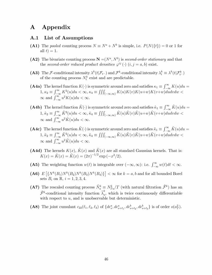
A Appendix

A.1 List of Assumptions

(A1) The pooled counting process N � Na +N b is simple, i.e. P (N(ftg) = 0 or 1 forall t) = 1.

(A2) The bivariate counting processN =(Na; N b) is second-order stationary and thatthe second-order reduced product densities 'ij (�) (i; j = a; b) exist.

(A3) TheF-conditional intensity �k(tjFt�) andFk-conditional intensity �kt � �k(tjFkt�)

of the counting process Nkt exist and are predictable.

(A4a) The kernel functionK(�) is symmetric around zero and satis�es �1 �R1�1K(u)du =

1, �2 �R1�1K

2(u)du <1, �4 �RRR

(�1;1)K(u)K(v)K(u+w)K(v+w)dudvdw <

1 andR1�1 u

2K(u)du <1.

(A4b) The kernel function �K(�) is symmetric around zero and satis�es��1 �R1�1

�K(u)du =

1,��2 �R1�1

�K2(u)du <1,��4 �RRR

(�1;1)�K(u)�K(v)�K(u+w)�K(v+w)dudvdw <

1 andR1�1 u

2�K(u)du <1.

(A4c) The kernel function �K(�) is symmetric around zero and satis�es ��1 �R1�1

�K(u)du =

1, ��2 �R1�1

�K2(u)du <1, ��4 �RRR

(�1;1)�K(u) �K(v) �K(u+w) �K(v+w)dudvdw <

1 andR1�1 u

2 �K(u)du <1.

(A4d) The kernels K(x), �K(x) and �K(x) are all standard Gaussian kernels. That is:K(x) = �K(x) = �K(x) = (2�)�1=2 exp (�x2=2).

(A5) The weighting function w(`) is integrable over (�1;1): i.e.R1�1w(`)d` <1.

(A6) E�fNk(B1)N

k(B2)Nk(B3)N

k(B4)g�<1 for k = a; b and for all bounded Borel

sets Bi on R, i = 1; 2; 3; 4.

(A7) The rescaled counting process ~Nku � Nk

Tu=T (with natural �ltration ~Fk) has an~Fk-conditional intensity function ~�

k

u, which is twice continuously di¤erentiablewith respect to u, and is unobservable but deterministic.

(A8) The joint cumulant c22(`1; `2; `3) of fd�as ; d�as+`1 ; d�bs+`2

; d�bs+`3g is of order o(a2T ).

46

A.2 Figures

Figure 1: The statistic Q aggregates the squared contributions of residual productsd�asd�

bt for all s < t. The lines join all pairs of type a and type b events (shocks) at

their event times (�ai ; �aj ) for all �

ai < �

aj .

(a) T = 500; B = 10;M = 60 (b) T = 1000; B = 10;M = 75

(c) T = 1500; B = 10;M = 100 (d) T = 2000; B = 10;M = 120

Figure 2: Size experiment of Q test, bivariate Poisson process.Runs=5000, DGP= bivariate Poisson process (two independent Poisson processes with rate 0.1). Nominal size: blue=0.1;

red=0.05; green=0.025; black=0.01.

47

(a) size: H = 3; B = 2 (b) power: H = 3; B = 2

(c) size: H = 3; B = 20 (d) power: H = 3; B = 20

Figure 3: Size and power experiment of Q test, bivariate exponential Hawkes process.Runs=10000, T=1800, DGP= bivariate exponential Hawkes model in (23). Nominal size: blue=0.1; red=0.05;

green=0.025; black=0.01.

48

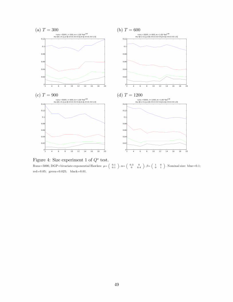
(a) T = 300 (b) T = 600

2 4 6 8 10 12 14 16 18 200

0.02

0.04

0.06

0.08

0.1

0.12

 runs  = 5000,  t = 300, m = 1.00 *bw1.00

 mu=[0.1 0.1], a=[0.3 0.0; 0.0 0.4], b=[1.0 0.0; 0.0 1.0]

2 4 6 8 10 12 14 16 18 200

0.02

0.04

0.06

0.08

0.1

0.12

 runs  = 5000,  t = 600, m = 1.00 *bw1.00

 mu=[0.1 0.1], a=[0.3 0.0; 0.0 0.4], b=[1.0 0.0; 0.0 1.0]

(c) T = 900 (d) T = 1200

2 4 6 8 10 12 14 16 18 200

0.02

0.04

0.06

0.08

0.1

0.12

0.14

 runs  = 5000,  t = 900, m = 1.00 *bw1.00

 mu=[0.1 0.1], a=[0.3 0.0; 0.0 0.4], b=[1.0 0.0; 0.0 1.0]

2 4 6 8 10 12 14 16 18 200

0.02

0.04

0.06

0.08

0.1

0.12

0.14

 runs  = 5000,  t = 1200, m = 1.00 *bw1.00

 mu=[0.1 0.1], a=[0.3 0.0; 0.0 0.4], b=[1.0 0.0; 0.0 1.0]

Figure 4: Size experiment 1 of Qs test.Runs=5000, DGP=bivariate exponential Hawkes: �=

�0:10:1

�, �=

�0:3 00 0:4

�, �=

�1 00 1

�: Nominal size: blue=0.1;

red=0.05; green=0.025; black=0.01.

49

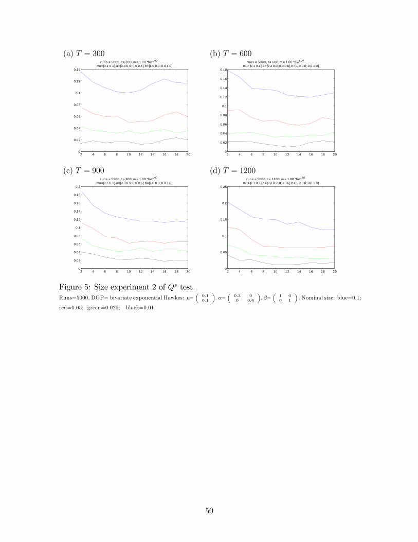
(a) T = 300 (b) T = 600

2 4 6 8 10 12 14 16 18 200

0.02

0.04

0.06

0.08

0.1

0.12

0.14

 runs  = 5000,  t = 300, m = 1.00 *bw1.00

 mu=[0.1 0.1], a=[0.3 0.0; 0.0 0.6], b=[1.0 0.0; 0.0 1.0]

2 4 6 8 10 12 14 16 18 200

0.02

0.04

0.06

0.08

0.1

0.12

0.14

0.16

0.18

 runs  = 5000,  t = 600, m = 1.00 *bw1.00

 mu=[0.1 0.1], a=[0.3 0.0; 0.0 0.6], b=[1.0 0.0; 0.0 1.0]

(c) T = 900 (d) T = 1200

2 4 6 8 10 12 14 16 18 200

0.02

0.04

0.06

0.08

0.1

0.12

0.14

0.16

0.18

0.2

 runs  = 5000,  t = 900, m = 1.00 *bw1.00

 mu=[0.1 0.1], a=[0.3 0.0; 0.0 0.6], b=[1.0 0.0; 0.0 1.0]

2 4 6 8 10 12 14 16 18 200

0.05

0.1

0.15

0.2

0.25

 runs  = 5000,  t = 1200, m = 1.00 *bw1.00

 mu=[0.1 0.1], a=[0.3 0.0; 0.0 0.6], b=[1.0 0.0; 0.0 1.0]

Figure 5: Size experiment 2 of Qs test.Runs=5000, DGP= bivariate exponential Hawkes: �=

�0:10:1

�, �=

�0:3 00 0:6

�, �=

�1 00 1

�: Nominal size: blue=0.1;

red=0.05; green=0.025; black=0.01.

50

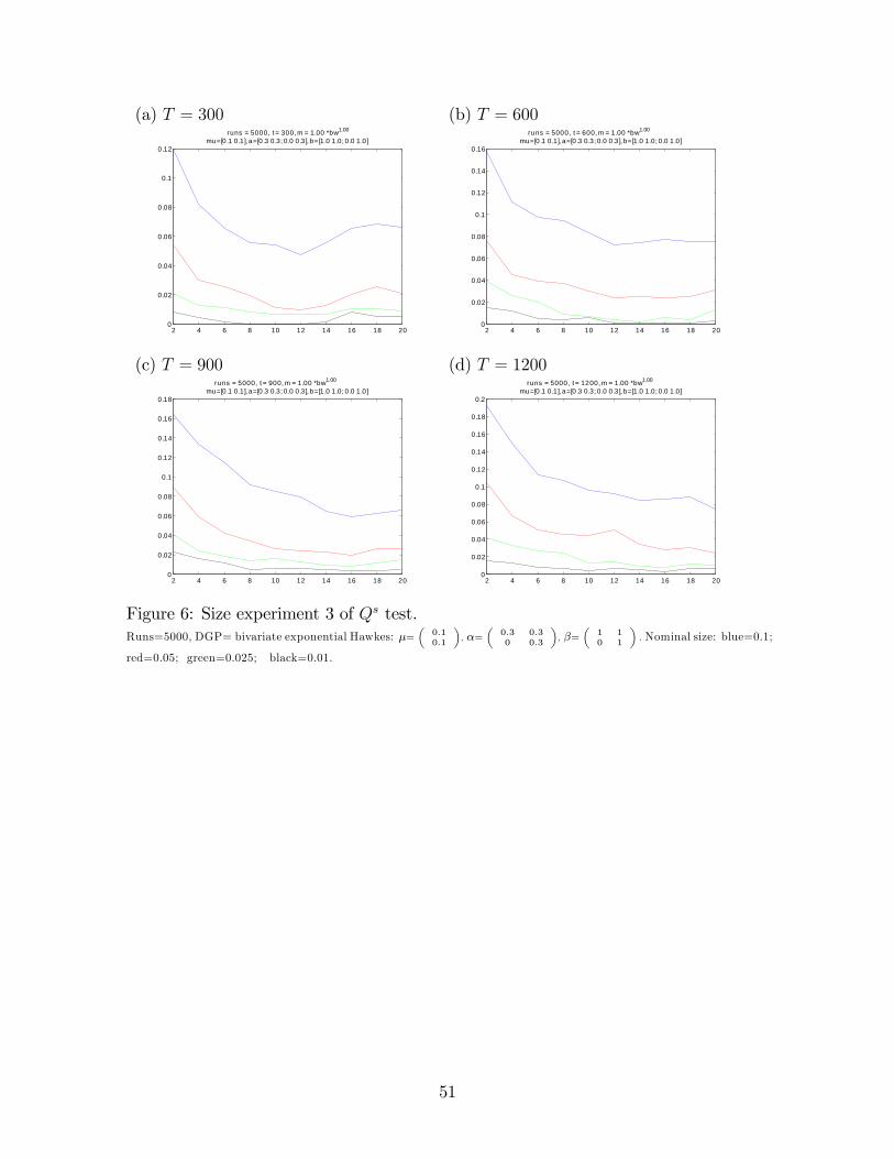
(a) T = 300 (b) T = 600

2 4 6 8 10 12 14 16 18 200

0.02

0.04

0.06

0.08

0.1

0.12

 runs  = 5000,  t = 300, m = 1.00 *bw1.00

 mu=[0.1 0.1], a=[0.3 0.3; 0.0 0.3], b=[1.0 1.0; 0.0 1.0]

2 4 6 8 10 12 14 16 18 200

0.02

0.04

0.06

0.08

0.1

0.12

0.14

0.16

 runs  = 5000,  t = 600, m = 1.00 *bw1.00

 mu=[0.1 0.1], a=[0.3 0.3; 0.0 0.3], b=[1.0 1.0; 0.0 1.0]

(c) T = 900 (d) T = 1200

2 4 6 8 10 12 14 16 18 200

0.02

0.04

0.06

0.08

0.1

0.12

0.14

0.16

0.18

 runs  = 5000,  t = 900, m = 1.00 *bw1.00

 mu=[0.1 0.1], a=[0.3 0.3; 0.0 0.3], b=[1.0 1.0; 0.0 1.0]

2 4 6 8 10 12 14 16 18 200

0.02

0.04

0.06

0.08

0.1

0.12

0.14

0.16

0.18

0.2

 runs  = 5000,  t = 1200, m = 1.00 *bw1.00

 mu=[0.1 0.1], a=[0.3 0.3; 0.0 0.3], b=[1.0 1.0; 0.0 1.0]

Figure 6: Size experiment 3 of Qs test.Runs=5000, DGP= bivariate exponential Hawkes: �=

�0:10:1

�, �=

�0:3 0:30 0:3

�, �=

�1 10 1

�: Nominal size: blue=0.1;

red=0.05; green=0.025; black=0.01.

51

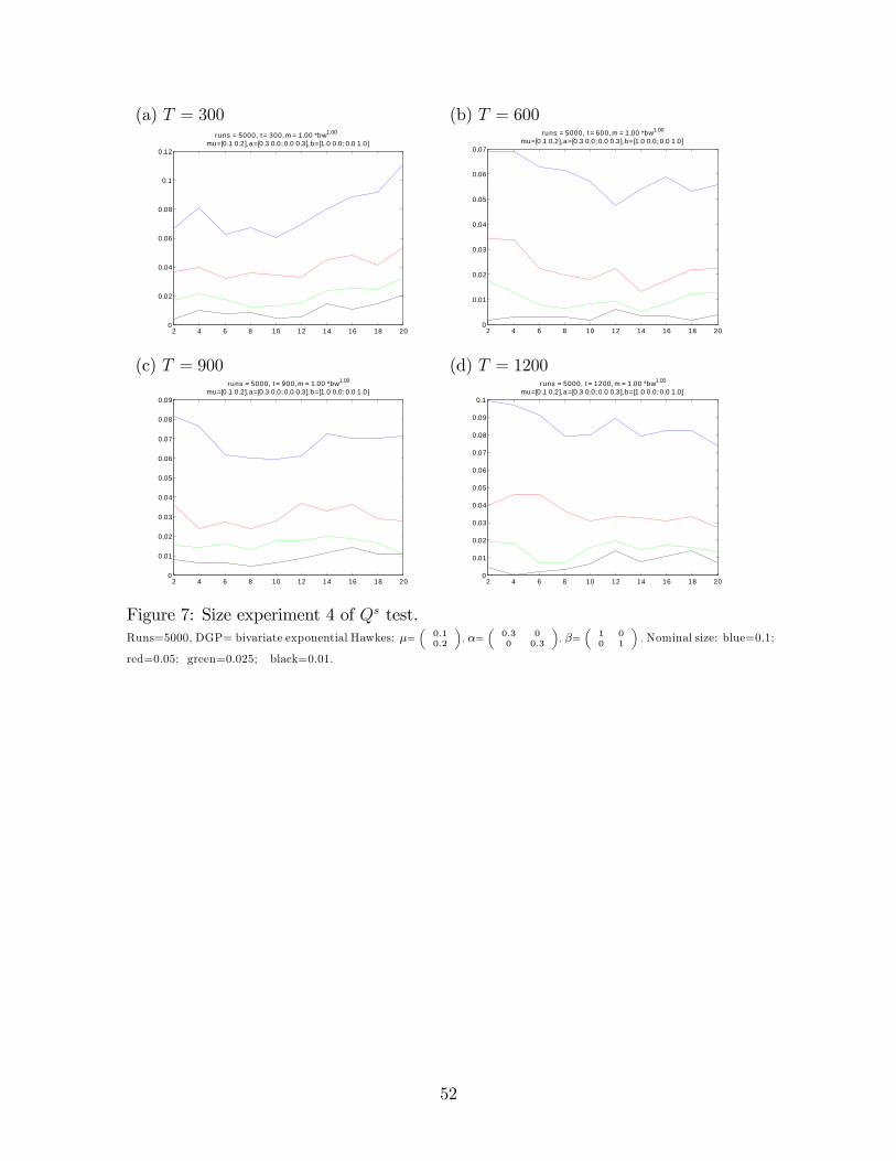
(a) T = 300 (b) T = 600

2 4 6 8 10 12 14 16 18 200

0.02

0.04

0.06

0.08

0.1

0.12

 runs  = 5000,  t = 300, m = 1.00 *bw1.00

 mu=[0.1 0.2], a=[0.3 0.0; 0.0 0.3], b=[1.0 0.0; 0.0 1.0]

2 4 6 8 10 12 14 16 18 200

0.01

0.02

0.03

0.04

0.05

0.06

0.07

 runs  = 5000,  t = 600, m = 1.00 *bw1.00

 mu=[0.1 0.2], a=[0.3 0.0; 0.0 0.3], b=[1.0 0.0; 0.0 1.0]

(c) T = 900 (d) T = 1200

2 4 6 8 10 12 14 16 18 200

0.01

0.02

0.03

0.04

0.05

0.06

0.07

0.08

0.09

 runs  = 5000,  t = 900, m = 1.00 *bw1.00

 mu=[0.1 0.2], a=[0.3 0.0; 0.0 0.3], b=[1.0 0.0; 0.0 1.0]

2 4 6 8 10 12 14 16 18 200

0.01

0.02

0.03

0.04

0.05

0.06

0.07

0.08

0.09

0.1

 runs  = 5000,  t = 1200, m = 1.00 *bw1.00

 mu=[0.1 0.2], a=[0.3 0.0; 0.0 0.3], b=[1.0 0.0; 0.0 1.0]

Figure 7: Size experiment 4 of Qs test.Runs=5000, DGP= bivariate exponential Hawkes: �=

�0:10:2

�, �=

�0:3 00 0:3

�, �=

�1 00 1

�: Nominal size: blue=0.1;

red=0.05; green=0.025; black=0.01.

52

(a) T = 300 (b) T = 600

5 10 15 20 25 30 35 40 45 500

0.02

0.04

0.06

0.08

0.1

0.12

0.14

0.16

0.18

 runs  = 5000,  t = 300, m = 0.50 *bw1.00

 mu=[0.1 0.1], a=[0.9 0.0; 0.0 0.9], b=[1.0 0.0; 0.0 1.0]

10 20 30 40 50 60 70 80 90 1000

0.02

0.04

0.06

0.08

0.1

0.12

0.14

0.16

0.18

0.2

 runs  = 5000,  t = 600, m = 0.50 *bw1.00

 mu=[0.1 0.1], a=[0.9 0.0; 0.0 0.9], b=[1.0 0.0; 0.0 1.0]

(c) T = 900 (d) T = 1200

0 50 100 1500

0.02

0.04

0.06

0.08

0.1

0.12

0.14

0.16

0.18

 runs  = 5000,  t = 900, m = 0.50 *bw1.00

 mu=[0.1 0.1], a=[0.9 0.0; 0.0 0.9], b=[1.0 0.0; 0.0 1.0]

20 40 60 80 100 120 140 160 180 2000

0.02

0.04

0.06

0.08

0.1

0.12

0.14

0.16

0.18

 runs  = 5000,  t = 1200, m = 0.50 *bw1.00

 mu=[0.1 0.1], a=[0.9 0.0; 0.0 0.9], b=[1.0 0.0; 0.0 1.0]

Figure 8: Size experiment 5 of Qs test.Runs=5000, DGP= bivariate exponential Hawkes: �=

�0:10:1

�, �=

�0:9 00 0:9

�, �=

�1 00 1

�: Nominal size: blue=0.1;

red=0.05; green=0.025; black=0.01.

53

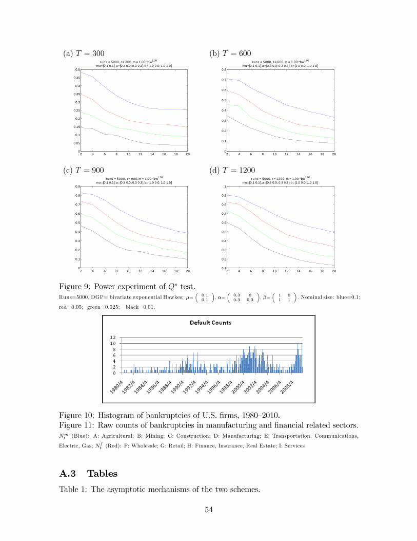
(a) T = 300 (b) T = 600

2 4 6 8 10 12 14 16 18 200

0.05

0.1

0.15

0.2

0.25

0.3

0.35

0.4

0.45

0.5

 runs  = 5000,  t = 300, m = 1.00 *bw1.00

 mu=[0.1 0.1], a=[0.3 0.0; 0.3 0.3], b=[1.0 0.0; 1.0 1.0]

2 4 6 8 10 12 14 16 18 200

0.1

0.2

0.3

0.4

0.5

0.6

0.7

0.8

 runs  = 5000,  t = 600, m = 1.00 *bw1.00

 mu=[0.1 0.1], a=[0.3 0.0; 0.3 0.3], b=[1.0 0.0; 1.0 1.0]

(c) T = 900 (d) T = 1200

2 4 6 8 10 12 14 16 18 200

0.1

0.2

0.3

0.4

0.5

0.6

0.7

0.8

0.9

 runs  = 5000,  t = 900, m = 1.00 *bw1.00

 mu=[0.1 0.1], a=[0.3 0.0; 0.3 0.3], b=[1.0 0.0; 1.0 1.0]

2 4 6 8 10 12 14 16 18 200.1

0.2

0.3

0.4

0.5

0.6

0.7

0.8

0.9

1

 runs  = 5000,  t = 1200, m = 1.00 *bw1.00

 mu=[0.1 0.1], a=[0.3 0.0; 0.3 0.3], b=[1.0 0.0; 1.0 1.0]

Figure 9: Power experiment of Qs test.Runs=5000, DGP= bivariate exponential Hawkes: �=

�0:10:1

�, �=

�0:3 00:3 0:3

�, �=

�1 01 1

�: Nominal size: blue=0.1;

red=0.05; green=0.025; black=0.01.

Figure 10: Histogram of bankruptcies of U.S. �rms, 1980�2010.Figure 11: Raw counts of bankruptcies in manufacturing and �nancial related sectors.Nmt (Blue): A: Agricultural; B: Mining; C: Construction; D: Manufacturing; E: Transportation, Communications,

Electric, Gas; Nft (Red): F: Wholesale; G: Retail; H: Finance, Insurance, Real Estate; I: Services

A.3 Tables

Table 1: The asymptotic mechanisms of the two schemes.

54

Scheme Observation window Sample size Limit Duration1 [0; T ] n = N(T ) T !1) n!1 � i � � i�1 �xed2 [0; T0] n = N(T0) n!1, T0 �xed � i � � i�1 # 0

Table 2: Signi�cant day counts (out of 41 days) of PG, 9:45am �10:15am.H B M Trade ! Quote Quote ! Tradesig. levels: 0.1 0.05 0.01 0.1 0.05 0.01

0.6 2 20 3 1 1 4 2 10.6 4 17 4 3 2 4 2 10.6 10 15 7 5 3 1 1 00.6 20 10 4 2 1 1 1 11 2 38 8 7 3 6 6 31 4 35 9 6 3 4 3 31 10 30 15 15 15 4 3 21 20 27 16 15 11 3 2 23 2 40 8 6 5 7 6 33 4 35 13 11 6 8 7 23 10 33 19 16 11 7 5 43 20 30 15 12 11 4 2 2Mean number of trades=88.8, quotes=325.1. The bandwidth combinations give right sizes in simulations (with an

estimated bivariate Hawkes model to PG data as DGP). Bandwidths (in days) of (i) cross-covariance function: H; (ii)

weighting function: B; (iii) conditional intensity: M . All kernels are Gaussian.

Table 3: Signi�cant day counts (out of 41 days) of PG, 11:45am �12:45pm.

55

H B M Trade ! Quote Quote ! Tradesig. levels: 0.1 0.05 0.01 0.1 0.05 0.01

0.6 2 20 11 8 6 8 6 40.6 4 17 16 15 11 9 7 40.6 10 15 17 16 15 8 6 50.6 20 10 9 6 6 7 5 31 2 38 6 5 4 8 8 61 4 35 20 18 13 10 8 71 10 30 17 16 13 11 10 81 20 27 17 16 14 13 11 93 2 40 14 9 4 17 12 63 4 35 24 20 18 19 14 113 10 33 26 25 22 24 20 183 20 30 25 23 18 26 25 16Mean number of trades=103.8, quotes=403.73. The bandwidth combinations give right sizes in simulations (with an

estimated bivariate Hawkes model to PG data as DGP). Bandwidths (in days) of (i) cross-covariance function: H; (ii)

weighting function: B; (iii) conditional intensity: M . All kernels are Gaussian.

Table 4: Signi�cant day counts (out of 41 days) of PG, 3:30pm �4:00pm.H B M Trade ! Quote Quote ! Tradesig. levels: 0.1 0.05 0.01 0.1 0.05 0.01

0.6 2 20 1 0 0 2 1 10.6 4 17 7 5 3 1 1 00.6 10 15 8 7 7 0 0 00.6 20 10 6 5 3 1 1 01 2 38 4 3 2 4 3 11 4 35 5 5 4 2 2 11 10 30 18 18 16 6 5 21 20 27 13 13 13 2 2 03 2 40 5 5 3 6 4 33 4 35 10 9 7 6 6 43 10 33 14 13 12 7 7 53 20 30 10 10 9 8 6 2Mean number of trades=93.7, quotes=361.56. The bandwidth combinations give right sizes in simulations (with an

estimated bivariate Hawkes model to PG data as DGP). Bandwidths (in days) of (i) cross-covariance function: H; (ii)

weighting function: B; (iii) conditional intensity: M . All kernels are Gaussian.

56

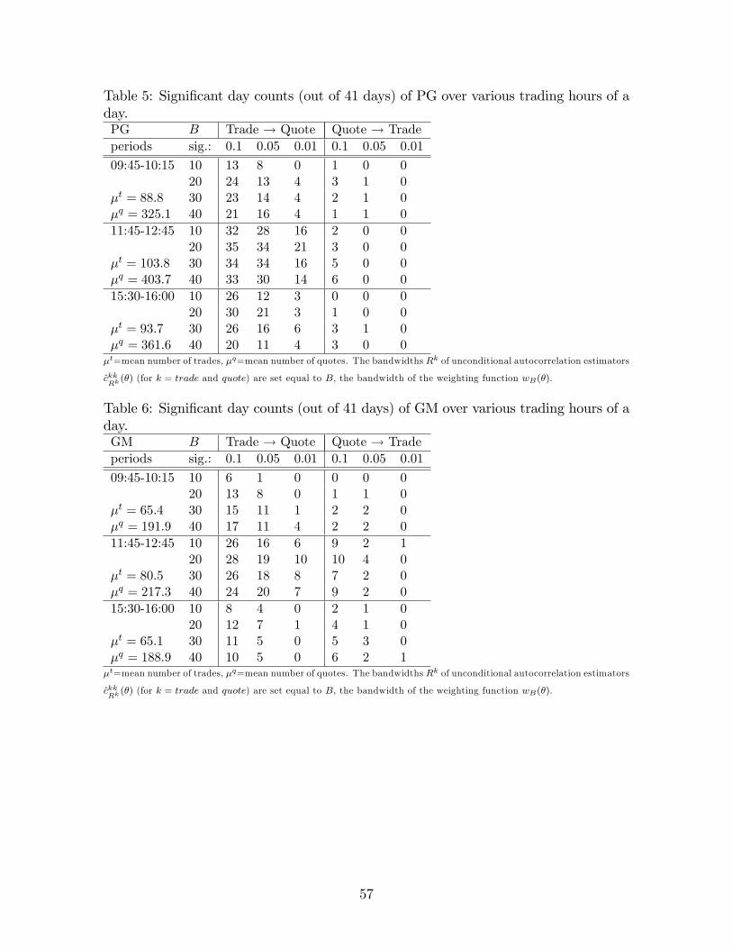
Table 5: Signi�cant day counts (out of 41 days) of PG over various trading hours of aday.PG B Trade ! Quote Quote ! Tradeperiods sig.: 0.1 0.05 0.01 0.1 0.05 0.01

09:45-10:15 10 13 8 0 1 0 020 24 13 4 3 1 0

�t = 88:8 30 23 14 4 2 1 0�q = 325:1 40 21 16 4 1 1 011:45-12:45 10 32 28 16 2 0 0

20 35 34 21 3 0 0�t = 103:8 30 34 34 16 5 0 0�q = 403:7 40 33 30 14 6 0 015:30-16:00 10 26 12 3 0 0 0

20 30 21 3 1 0 0�t = 93:7 30 26 16 6 3 1 0�q = 361:6 40 20 11 4 3 0 0�t=mean number of trades, �q=mean number of quotes. The bandwidths Rk of unconditional autocorrelation estimators

ckkRk(�) (for k = trade and quote) are set equal to B, the bandwidth of the weighting function wB(�).

Table 6: Signi�cant day counts (out of 41 days) of GM over various trading hours of aday.GM B Trade ! Quote Quote ! Tradeperiods sig.: 0.1 0.05 0.01 0.1 0.05 0.01

09:45-10:15 10 6 1 0 0 0 020 13 8 0 1 1 0

�t = 65:4 30 15 11 1 2 2 0�q = 191:9 40 17 11 4 2 2 011:45-12:45 10 26 16 6 9 2 1

20 28 19 10 10 4 0�t = 80:5 30 26 18 8 7 2 0�q = 217:3 40 24 20 7 9 2 015:30-16:00 10 8 4 0 2 1 0

20 12 7 1 4 1 0�t = 65:1 30 11 5 0 5 3 0�q = 188:9 40 10 5 0 6 2 1�t=mean number of trades, �q=mean number of quotes. The bandwidths Rk of unconditional autocorrelation estimators

ckkRk(�) (for k = trade and quote) are set equal to B, the bandwidth of the weighting function wB(�).

57

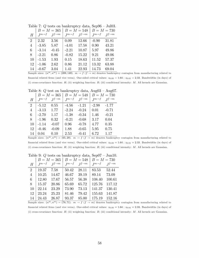
Table 7: Q tests on bankruptcy data, Sep96 �Jul03.B =M = 365 B =M = 548 B =M = 730

H Jm!f Jf!m Jm!f Jf!m Jm!f Jf!m

2 2.32 3.56 0.09 12.66 -0.90 31.814 -3.85 5.87 -4.01 17.58 0.90 43.216 -3.14 -0.45 -2.21 10.87 5.97 49.868 -2.21 0.86 -0.82 15.22 9.21 49.0610 -1.53 1.93 0.15 18.63 11.52 57.3712 -1.06 2.62 0.86 21.12 13.32 63.8814 -0.67 3.04 1.41 22.93 14.73 69.04Sample sizes: (nm; nm) = (209; 149). m ! f (f ! m) denotes bankruptcy contagion from manufacturing related to

�nancial related �rms (and vice versa). One-sided critical values: z0:05 = 1:64 ; z0:01 = 2:33. Bandwidths (in days) of

(i) cross-covariance function: H; (ii) weighting function: B; (iii) conditional intensity: M . All kernels are Gaussian.

Table 8: Q test on bankruptcy data, Aug03 �Aug07.B =M = 365 B =M = 548 B =M = 730

H Jm!f Jf!m Jm!f Jf!m Jm!f Jf!m

2 -5.12 0.55 -4.56 -1.21 -2.98 -1.774 -3.13 1.77 -2.24 -0.24 0.01 -0.716 -2.70 1.17 -1.38 -0.34 1.46 -0.218 -1.96 0.32 -0.21 -0.68 3.17 0.0410 -1.14 -0.07 0.96 -0.78 4.77 0.3512 -0.46 -0.09 1.88 -0.65 5.95 0.7514 0.04 0.10 2.53 -0.41 6.72 1.17Sample sizes: (nm; nm) = (65; 29). m ! f (f ! m) denotes bankruptcy contagion from manufacturing related to

�nancial related �rms (and vice versa). One-sided critical values: z0:05 = 1:64 ; z0:01 = 2:33. Bandwidths (in days) of

(i) cross-covariance function: H; (ii) weighting function: B; (iii) conditional intensity: M . All kernels are Gaussian.

Table 9: Q tests on bankruptcy data, Sep07 �Jun10.B =M = 365 B =M = 548 B =M = 730

H Jm!f Jf!m Jm!f Jf!m Jm!f Jf!m

2 19.37 7.58 50.42 28.11 83.53 52.444 10.25 14.67 46.67 39.19 89.14 73.096 12.80 17.67 56.57 56.38 108.40 100.618 15.37 20.86 65.69 65.72 125.76 117.1210 22.14 23.29 73.90 73.13 141.37 130.4112 23.24 25.23 81.46 79.42 155.63 141.8714 24.43 26.87 93.37 85.00 175.19 152.16Sample sizes: (nm; nm) = (78; 71). m ! f (f ! m) denotes bankruptcy contagion from manufacturing related to

�nancial related �rms (and vice versa). One-sided critical values: z0:05 = 1:64 ; z0:01 = 2:33. Bandwidths (in days) of

(i) cross-covariance function: H; (ii) weighting function: B; (iii) conditional intensity: M . All kernels are Gaussian.

58

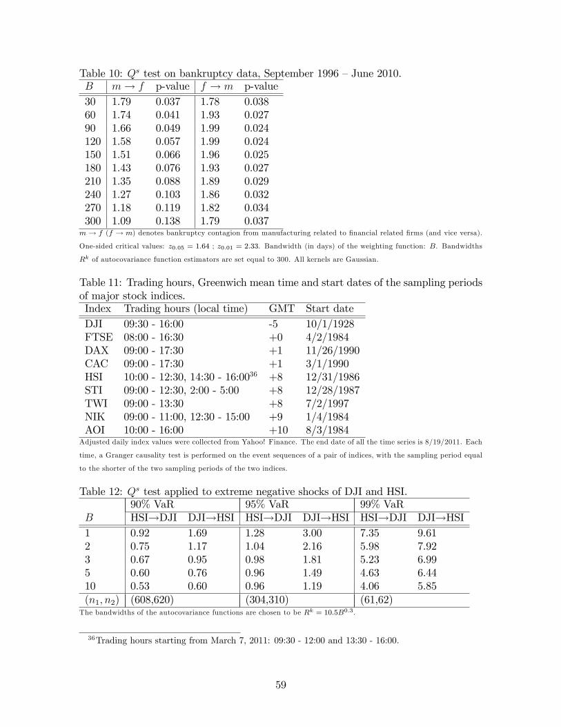
Table 10: Qs test on bankruptcy data, September 1996 �June 2010.B m! f p-value f ! m p-value30 1.79 0.037 1.78 0.03860 1.74 0.041 1.93 0.02790 1.66 0.049 1.99 0.024120 1.58 0.057 1.99 0.024150 1.51 0.066 1.96 0.025180 1.43 0.076 1.93 0.027210 1.35 0.088 1.89 0.029240 1.27 0.103 1.86 0.032270 1.18 0.119 1.82 0.034300 1.09 0.138 1.79 0.037m! f (f ! m) denotes bankruptcy contagion from manufacturing related to �nancial related �rms (and vice versa).

One-sided critical values: z0:05 = 1:64 ; z0:01 = 2:33. Bandwidth (in days) of the weighting function: B. Bandwidths

Rk of autocovariance function estimators are set equal to 300. All kernels are Gaussian.

Table 11: Trading hours, Greenwich mean time and start dates of the sampling periodsof major stock indices.Index Trading hours (local time) GMT Start dateDJI 09:30 - 16:00 -5 10/1/1928FTSE 08:00 - 16:30 +0 4/2/1984DAX 09:00 - 17:30 +1 11/26/1990CAC 09:00 - 17:30 +1 3/1/1990HSI 10:00 - 12:30, 14:30 - 16:0036 +8 12/31/1986STI 09:00 - 12:30, 2:00 - 5:00 +8 12/28/1987TWI 09:00 - 13:30 +8 7/2/1997NIK 09:00 - 11:00, 12:30 - 15:00 +9 1/4/1984AOI 10:00 - 16:00 +10 8/3/1984Adjusted daily index values were collected from Yahoo! Finance. The end date of all the time series is 8/19/2011. Each

time, a Granger causality test is performed on the event sequences of a pair of indices, with the sampling period equal

to the shorter of the two sampling periods of the two indices.

Table 12: Qs test applied to extreme negative shocks of DJI and HSI.90% VaR 95% VaR 99% VaR

B HSI!DJI DJI!HSI HSI!DJI DJI!HSI HSI!DJI DJI!HSI1 0.92 1.69 1.28 3.00 7.35 9.612 0.75 1.17 1.04 2.16 5.98 7.923 0.67 0.95 0.98 1.81 5.23 6.995 0.60 0.76 0.96 1.49 4.63 6.4410 0.53 0.60 0.96 1.19 4.06 5.85(n1; n2) (608,620) (304,310) (61,62)The bandwidths of the autocovariance functions are chosen to be Rk = 10:5B0:3.

36Trading hours starting from March 7, 2011: 09:30 - 12:00 and 13:30 - 16:00.

59

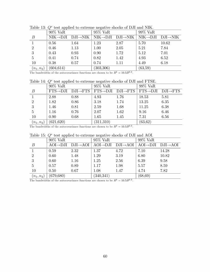
Table 13: Qs test applied to extreme negative shocks of DJI and NIK.90% VaR 95% VaR 99% VaR

B NIK!DJI DJI!NIK NIK!DJI DJI!NIK NIK!DJI DJI!NIK1 0.56 1.64 1.23 2.87 5.70 10.622 0.46 1.13 1.00 2.05 5.21 7.843 0.43 0.93 0.90 1.72 5.12 7.015 0.41 0.74 0.82 1.42 4.93 6.5210 0.38 0.57 0.74 1.11 4.49 6.18(n1; n2) (604,614) (303,306) (63,59)The bandwidths of the autocovariance functions are chosen to be Rk = 10:5B0:3.

Table 14: Qs test applied to extreme negative shocks of DJI and FTSE.90% VaR 95% VaR 99% VaR

B FTS!DJI DJI!FTS FTS!DJI DJI!FTS FTS!DJI DJI!FTS1 2.88 0.88 4.93 1.76 18.53 5.812 1.82 0.86 3.18 1.74 13.25 6.353 1.46 0.81 2.59 1.68 11.25 6.385 1.16 0.76 2.07 1.62 9.16 6.4610 0.90 0.68 1.65 1.45 7.31 6.56(n1; n2) (621,620) (311,310) (63,62)The bandwidths of the autocovariance functions are chosen to be Rk = 10:5B0:3.

Table 15: Qs test applied to extreme negative shocks of DJI and AOI.90% VaR 95% VaR 99% VaR

B AOI!DJI DJI!AOI AOI!DJI DJI!AOI AOI!DJI DJI!AOI1 0.59 2.32 1.37 4.72 7.10 14.282 0.60 1.48 1.29 3.19 6.80 10.823 0.60 1.16 1.25 2.56 6.39 9.585 0.57 0.89 1.17 1.98 5.57 8.5910 0.50 0.67 1.08 1.47 4.74 7.82(n1; n2) (679,680) (340,341) (68,69)The bandwidths of the autocovariance functions are chosen to be Rk = 10:5B0:3.

60

A.4 Proof of Theorem 5

I �rst expand (12) into

H(`) = 1TH

Z T

0

Z T

0

K�t�s�`H

� �dNa

s � �a

sds��dN b

t � �b

tdt�

= 1TH

Z T

0

Z T

0

K�t�s�`H

� hdNa

s dNbt � �

a

sdsdNbt � dNa

s �b

tdt+ �a

s �b

tdsdti

= A1 + A2 + A3 + A4: (24)

The �rst term is

A1 =1TH

NaTP

i=1

NbTP

j=1

K�tbj�tai�`H

�:

The second term, after substituting �b

t by (14), becomes

A2 = � 1THM

NaTP

i=1

NbTP

j=1

Z T

0

K�tbj�s�`H

��K�s�taiM

�ds:

Similarly, the third term is

A3 = � 1THM

NaTP

i=1

NbTP

j=1

Z T

0

K�t�tai�`H

��K�tbj�tM

�dt;

and the fourth one is

A4 =1

THM2

NaTP

i=1

NbTP

j=1

Z T

0

Z T

0

K�t�s�`H

��K�s�taiM

��K�tbj�tM

�dsdt:

Note that the last three terms involve the convolution of the kernels K(�) and �K(�)(twice for A4).Under assumption (A4d), I can simplify the expressions further, as it is well known

that Gaussian kernels are invariant under convolution: for anyH1; H2 > 0, the Gaussiankernel K(�) enjoys the property that

1H1H2

Z 1

�1K�x�zH1

�K�zH2

�dz = 1p

H21+H

22

K

�xp

H21+H

22

�:

Using this invariance property and a change of variables, I can simplify the integrationsand rewrite (24) as

H(`) =1T

NaTP

i=1

NbTP

j=1

h1HK�tbj�tai�`H

�� 2p

H2+M2K�

tbj�tai�`pH2+M2

�+ 1p

H2+2M2K�

tbj�tai�`pH2+2M2

�i:

61

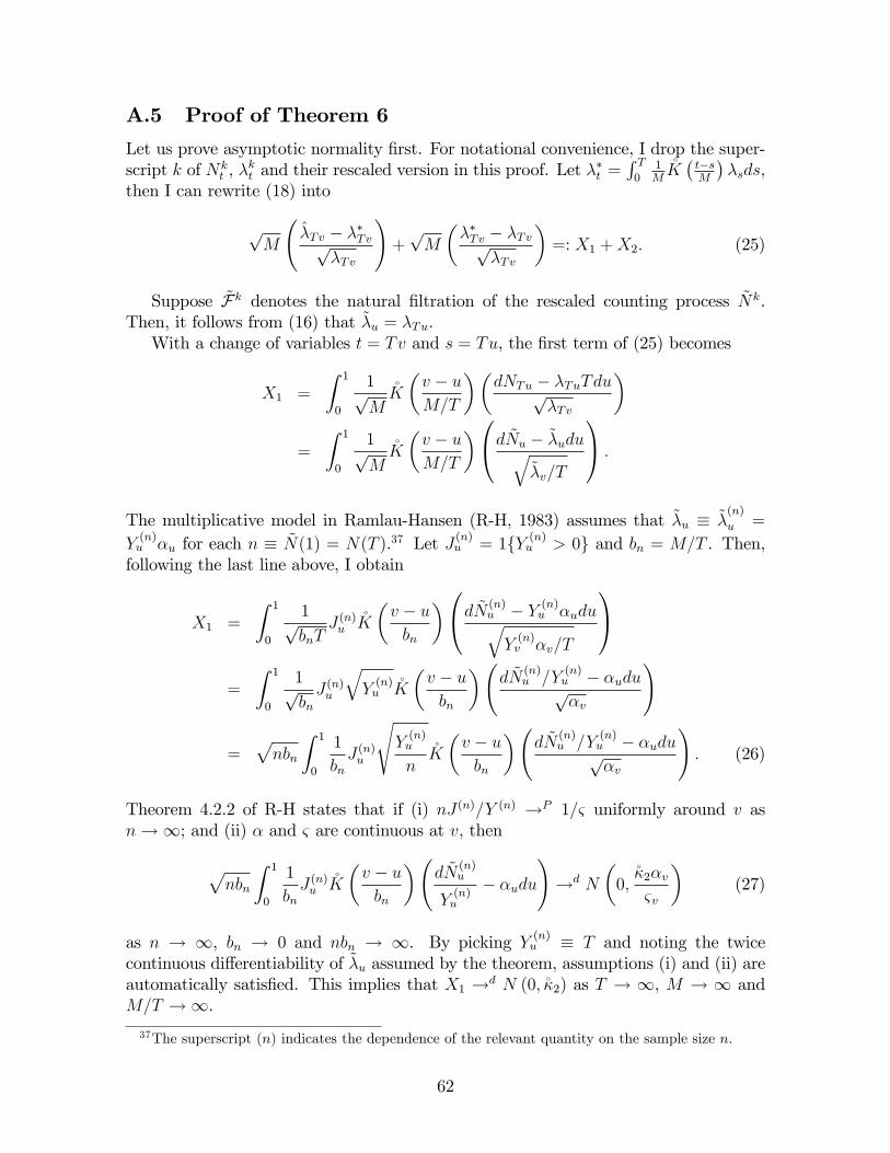
A.5 Proof of Theorem 6

Let us prove asymptotic normality �rst. For notational convenience, I drop the super-script k of Nk

t , �kt and their rescaled version in this proof. Let �

�t =

R T0

1M�K�t�sM

��sds,

then I can rewrite (18) into

pM

�Tv � ��Tvp

�Tv

!+pM

���Tv � �Tvp

�Tv

�=: X1 +X2: (25)

Suppose ~Fk denotes the natural �ltration of the rescaled counting process ~Nk.Then, it follows from (16) that ~�u = �Tu.With a change of variables t = Tv and s = Tu, the �rst term of (25) becomes

X1 =

Z 1

0

1pM�K

�v � uM=T

��dNTu � �TuTdup

�Tv

�

=

Z 1

0

1pM�K

�v � uM=T

�0@d ~Nu � ~�uduq~�v=T

1A :The multiplicative model in Ramlau-Hansen (R-H, 1983) assumes that ~�u � ~�

(n)

u =

Y(n)u �u for each n � ~N(1) = N(T ).37 Let J (n)u = 1fY (n)u > 0g and bn = M=T . Then,following the last line above, I obtain

X1 =

Z 1

0

1pbnT

J (n)u�K

�v � ubn

�0@d ~N (n)u � Y (n)u �uduqY(n)v �v=T

1A=

Z 1

0

1pbnJ (n)u

qY(n)u�K

�v � ubn

� d ~N

(n)u =Y

(n)u � �udup�v

!

=pnbn

Z 1

0

1

bnJ (n)u

sY(n)u

n�K

�v � ubn

� d ~N

(n)u =Y

(n)u � �udup�v

!: (26)

Theorem 4.2.2 of R-H states that if (i) nJ (n)=Y (n) !P 1=& uniformly around v asn!1; and (ii) � and & are continuous at v, then

pnbn

Z 1

0

1

bnJ (n)u

�K

�v � ubn

� d ~N

(n)u

Y(n)u

� �udu!!d N

�0;��2�v&v

�(27)

as n ! 1, bn ! 0 and nbn ! 1. By picking Y (n)u � T and noting the twicecontinuous di¤erentiability of ~�u assumed by the theorem, assumptions (i) and (ii) areautomatically satis�ed. This implies that X1 !d N (0;��2) as T ! 1, M ! 1 andM=T !1.37The superscript (n) indicates the dependence of the relevant quantity on the sample size n.

62

To complete the proof, it su¢ ces to show that the second term X2 of (25) is as-ymptotically negligible relative to the �rst term, which was just shown to be OP (1).Indeed, by symmetry of the kernel �K() and the twice continuous di¤erentiability of ~�u,I obtain

��Tv � �Tv =1

T

Z 1

0

T

M�K

�v � uM=T

��TuTdu� �Tv

=

Z 1

0

1

m�K

�v � um

�~�udu� �Tv

=

Z 1

0

�K (x) ~�v�mxdx� �Tv

= ~�v � �Tv +m~�0v

Z 1

0

x�K (x) dx+OP (m2)

= OP

�M

T

�2!:

If M5=T 4 ! 0 (which corresponds to nb5n ! 0), then X2 =pM (��Tv � �Tv) =

p�Tv =

OP (M2:5=T 2) = oP (1), and thus is asymptotically negligible relative to X1.

For mean-squared consistency of �Tv, simply apply Proposition 3.2.2 of R-H.

A.6 Proof of Theorem 7

For notational simplicity, I only treat the case where I = [0; T ]. Under the nullhypothesis, the innovations from the two processes are uncorrelated, which impliesthat E

�dNa

s dNbs+`

�= E (dNa

s )E�dN b

s+`

�= �a�bdsd`, so that

E (Qs) =1

T 2

ZI

ZJ

wB (`)E�dNa

s dNbs+`

�=

�a�b

T 2

ZI

ZJ

wB (`) dsd`

=�a�b

T

ZI

wB (`)�1� j`j

T

�d`:

Before computing the variance, let us recall that the second-order reduced prod-uct density of Nk (which exists by assumption (A2)) was de�ned by 'kk(u)dtdu =E�dNk

t dNkt+u

�for u 6= 0, and the unconditional autocovariance density function can

thus be expressed as ckk(u)dtdu = E�dNk

t � �kdt)(dNkt+u � �kdu

�=h'kk(u)�

��k�2idtdu

for u 6= 0. Then, under the null hypothesis, I obtain

E((Qs)2) =1

T 4

ZZI2

ZZJ2wB (`1)wB (`2)E

�dNa

s1dNa

s2dN b

s1+`1dN b

s2+`2

�=

1

T 4

ZZI2

ZZJ2wB (`1)wB (`2)E

�dNa

s1dNa

s2

�E�dN b

s1+`1dN b

s2+`2

�:

63

I can decompose the di¤erential as follows:

E�dNa

s1dNa

s2dN b

s1+`1dN b

s2+`2

�= E

�dNa

s1dNa

s2

�E�dN b

s1+`1dN b

s2+`2

�=

�E�dNa

s1dNa

s2

�� (�a)2 ds1ds2

� hE�dN b

s1+`1dN b

s2+`2

����b�2d`1d`2

i+��b�2 �E�dNa

s1dNa

s2

�� (�a)2 ds1ds2

�d`1d`2

+(�a)2hE�dN b

s1+`1dN b

s2+`2

����b�2d`1d`2

ids1ds2

+(�a)2��b�2ds1ds2d`1d`2

= caa(s2 � s1)cbb(s2 � s1 + `2 � `1)ds1ds2d`1d`2+��b�2caa(s2 � s1)ds1ds2d`1d`2

+(�a)2 cbb(s2 � s1 + `2 � `1)ds1ds2d`1d`2+(�a)2

��b�2ds1ds2d`1d`2:

Note that the integral term associated with the last di¤erential is [E(Qs)]2, so that

V ar(Qs) =1

T 4

ZZI2

ZZJ2wB (`1)wB (`2) c

aa(s2 � s1)cbb(s2 � s1 + `2 � `1)ds1ds2d`1d`2

+1

T 4

ZZI2

ZZJ2wB (`1)wB (`2)

��b�2caa(s2 � s1)ds1ds2d`1d`2

+1

T 4

ZZI2

ZZJ2wB (`1)wB (`2) (�

a)2 cbb(s2 � s1 + `2 � `1)ds1ds2d`1d`2

= A1 + A2 + A3:

Suppose I = [0; T ]. I evaluate the three terms individually as follows.

(i) the �rst term becomes

A1 =2

T 4

Z T

0

Z `2

0

ZJ2

ZJ1

wB (`1)wB (`2) caa (s2 � s1) cbb (s2 � s1 + `2 � `1) ds1ds2d`1d`2:

where Ji = [0; T � `i] for i = 1; 2. With a change of variables

(s1; s2; `1; `2) 7! (v = s2 � s1; s2; u = `2 � `1; `2) ;

I can rewrite A1 into

A1 = 2T 4

Z T

0

Z T

u

Z T�`2

�T

Z T�`2

0

wB (`2 � u)wB (`2) caa (v) cbb (v + u) ds2dvd`2du

= 2T 3

Z T

0

Z T

u

wB (`2 � u)wB (`2)�1� `2

T

� Z T�`2

�Tcaa (v) cbb (v + u) dvd`2du:

To simplify further, I rely on the assumption that the bandwidth of w (`) � wB (`)

64

is small relative to T , i.e. B = o(T ). Then, the integralR T�`2�T caa (v) cbb (v + u) dv can

be well approximated by �(u) :=R T�T c

aa (v) cbb (v + u) dv, and hence

A1 � 2T 3

Z T

0

W2(u)� (u) du:

where we de�ned a new weighting function byW2(u) :=R TuwB (`� u)wB (`)

�1� `

T

�d`.

Figure 12 gives a plot of W2(u) when w (�) is a standard normal density function andT is large (T � 3).

(ii) With a change of variables (s1; s2) 7�! (v = s2 � s1; s2), the second term be-comes

A2 =(�b)

2

T 4

ZZI2

ZZJ2wB (`1)wB (`2)

a(s2 � s1)ds1ds2d`1d`2

=(�b)

2

T 4

Z T

0

Z T

0

wB (`1)wB (`2)

Z T�`2

�(T�`1)

Z v+T�`1

v

caa(v)ds2dvd`1d`2

=(�b)

2

T 3

Z T

0

Z T

0

wB (`1)wB (`2)�1� `1

T

� Z T�`2

�(T�`1)caa(v)dvd`1d`2:

To simplify further, I rely on the assumption that the bandwidth B of the weightingfunction wB (�) is small relative to T , i.e. B = o(T ). Then, the following holdsapproximately: Z T�`2

�(T�`1)caa(v)dv �

Z T

�Tcaa(v)dv:

As a result, we obtain

A2 �2(�b)

2

T 3!1

Z T

0

caa(v)dv

where I de�ned the constant !1 :=R T0wB (`)

�1� `

T

�d` =

R T=B0

w (u)�1� Bu

T

�du.

(iii) With a change of variables (s1; s2) 7�! (x = s2 � s1 + `2 � `1; s2), the thirdterm becomes

A3 = (�a)2

T 4

ZZI2

ZZJ2wB (`1)wB (`2) c

bb(s2 � s1 + `2 � `1)ds1ds2d`1d`2

= (�a)2

T 4

Z T

0

Z T

0

wB (`1)wB (`2)

Z T�`1

�(T�`2)

Z x+T�`1+`2�`1

x+`2�`1cbb(x)ds2dxd`1d`2

= (�a)2

T 3

Z T

0

Z T

0

wB (`1)wB (`2)�1� `1

T

� Z T�`1

�(T�`2)cbb(x)dxd`1d`2:

To simplify further, I rely on the assumption that the bandwidth B of the weightingfunction wB (�) is small relative to T , i.e. B = o(T ). Then, the following holds

65

approximately: Z T�`1

�(T�`2)cbb(v)dv �

Z T

�Tcbb(v)dv:

As a result, I obtain

A3 � 2(�a)2

T 3!1

Z T

0

cbb(v)dv:

Combining the above three terms Ai for i = 1; 2; 3, I obtain an approximation tothe variance of Qs:

V ar(Qs) � 2T 3

�Z T

0

W2(u)� (u) du+��b�2!1

Z T

0

caa(v)dv + (�a)2 !1

Z T

0

cbb(v)dv

�:

A.7 Proof of (21)

For notational convenience, I drop the superscript k from all relevant symbols through-out this proof. Let R=T ! 0 as T ! 1. I start by decomposing cR(`) � ckk

Rk(`) as

follows:

cR(`) = 1TR

Z T

0

Z T

0

�K�t�s�`R

� �dNs � NT

Tds� �dNt � NT

Tdt�

= 1TR

Z T

0

Z T

0

�K�t�s�`R

�dNsdNt � 1

TRNTT

Z T

0

Z T

0

�K�t�s�`R

�dsdNt

� 1TR

NTT

Z T

0

Z T

0

�K�t�s�`R

�dNa

s dt+1TR

NTTNTT

Z T

0

Z T

0

�K�t�s�`R

�dsdt

= : C1 + C2 + C3 + C4:

Now, the second term is

C2 = � 1TR

NTT

Z T

0

Z T

0

�K�t�s�`R

�dsdN b

t

= �NTT 2

NTPj=1

Z T

0

1R�K�tj�s�`R

�ds = �NT

T 2

NTPj=1

Z (tbj�`)=R

(tbj�T�`)=R�K (x) dx

= �NTT 2

NTPj=1

�1f`<tj<T+`g\[0;T ] + o(1)

�= �NT

T 2

�NT^(T+`) �N`_0

�+ o(1);

where the third equality made use of assumption (A4c). By stationarity of Nk, Iobserve that NT^(T+`) �N`_0 = T�j`j

TNT . Therefore, up to the leading term,

C2 = �N2T

T 2

�1� j`j

T

�:

66

Similarly, by stationarity of N b, the third term is, up to the leading term,

C3 = �N2T

T 2

�1� j`j

T

�= C2:

The last term is

C4 = 1TNTTNTT

Z T

0

Z T

0

1R�K�t�s�`R

�dsdt

=N2T

T 21T

Z T

0

Z (t�`)=R

(t�T�`)=R�K (x) dxdt

=N2T

T 21T

Z T

0

�1f0<t�`<Tg\[0;T ] + o(1)

�dt

=N2T

T 2

�1� j`j

T

�+ o(1);

which is �C2 (neglecting the o(1) terms). As a result, except for the o(1) terms, Iobtain

cR(`) =1TR

NTPi=1

NTPj=1

�K�tj�ti�`R

�� N2

T

T 2

�1� j`j

T

�;

which is (21).

A.8 Proof of Theorem 8

Let d�kt = dNkt � �

k

t dt for k = a; b. Then,

Q =

ZI

wB(`) 2H(`)d`

=

ZI

wB(`)1

(TH)2

ZZZZ(0;T ]4

K�t1�s1�`

H

�K�t2�s2�`

H

�d�as1d�

as2d�bt1d�

bt2d`

= 1T 2

ZZZZ(0;T ]4

ZI

w(`) 1H2K

�t1�s1�`

H

�K�t2�s2�`

H

�d`d�as1d�

as2d�bt1d�

bt2

A.8.1 Asymptotic Mean of Q

By Fubini�s theorem, the expectation ofQ becomes an multiple integration with respectto E[d�as1d�

as2d�bs1+ud�

bs2+u

], which, under the null hypothesis (11), can be split intoE[d�as1d�

as2]E�d�bs1+ud�

bs2+u

�. By the law of iterated expectations and the martingale

property of the innovations d�ku, it follows that E[d�ku1d�ku2 ] = 0 unless u1 = u2 = u

67

when it is equal to E[�d�ku�2]. Then, I can simplify the di¤erential

�d�ku�2as follows:

�d�ku�2

=�dNk

u � �k

udu�2

=�dNk

u � �kudu+ �kudu� �k

udu�2

=�dNk

u � �kudu�2+��kudu� �

k

udu�2+ 2

�dNk

u � �kudu� ��kudu� �

k

udu�

=�dNk

u � �kudu�2+ oP (du)

= dNku � 2dNk

u�kudu+

��kudu

�2+ oP (du)

= dNku + oP (du): (28)

The second-to-last equality holds because of assumption (A1), which implies that�dNk

u

�2= dNk

u almost surely; hence the second order di¤erential�d�ku�2has a domi-

nating �rst-order increment dNku . It is therefore true, up to OP (du), that E[

�d�ku�2] =

E[dNku ] = �

kdu.Now, letting b = B=T and h = H=T , the expected value of Q is evaluated as follows:

E (Q) = 1T 2H2

ZZ(0;T ]2

ZI

wB(`)K2�t�s�`H

�d`�a�bdsdt

= T 3

T 2H2

ZZ(0;1]2

ZI=T

wB(T�)K2�v�u��H=T

�d��a�bdudv

= 1T 2h2

ZZ(0;1]2

ZI=T

wb(�)K2�v�u��h

�d��a�bdudv

Then, as h! 0, ZZ(0;1]2

1h2K2�v�u��h

�dudv

= 1h

Z 1

0

Z (v��)=h

(v�1��)=hK2 (x) dxdv

= 1h

Z 1

0

1f0<v��<1g\[0;1]dv

Z 1

�1K2(x)dx+ o

�1h

�= 1

h(1� j�j)�2 + o

�1h

�:

where �2 =R1�1K

2(x)dx (from assumption (A4a)). As a result, as T ! 1, Th =H ! 1 and h = H=T ! 0, the asymptotic mean of Q under the null hypothesis is

68

given by

E (Q) = 1T 2h�a�b�2

ZI=T

wb(�) (1� j�j) d� + o�

1T 2h

�= 1

T 2h�a�b�2

ZI

1bw( `

bT)�1� j`j

T

�1Td`+ o

�1T 2h

�= 1

TH�a�b�2

ZI

wB(`)�1� j`j

T

�d`+ o

�1TH

�: (29)

From (28), I also observe that�d�ku�2=�d�ku�2+oP (du), which entails that E(Q) =

E( ~Q).

A.8.2 Asymptotic Variance of Q Under the Null

The Case Without Autocorrelations Now, I derive the asymptotic variance ofQ as T ! 1, and H=T ! 0 as H ! 1. Let I � [c1; c2] � [�T; T ], where c1 < c2.Consider

E�Q2�= 1

(TH)4

ZZI2w(`1)w(`2)

Z� � �Z(0;T ]8

K�t11�s11�`1

H

�K�t21�s21�`1

H

�K�t12�s12�`2

H

�K�t22�s22�`2

H

�E�d�as11d�

as12d�bt11d�

bt12d�as21d�

as22d�bt21d�

bt22

�d`1d`2:

Assume that (i) there is no cross-correlation between the two innovation processes,i.e. (u) = 0; and (ii) there is no auto-correlation for each component process, i.e.caa(u) = cbb(u) = 0. I will relax the second assumption in the next subsection.A key observation is that E (Q2) 6= 0 only in the following cases (in all cases

s1 6= s2 6= t1 6= t2 and s 6= t):

1. R1 = fs11 = s12 = s1, s21 = s22 = s2 , t11 = t12 = t1, t21 = t22 = t2g;

2. R2 = fs11 = s12 = s1, s21 = s22 = s2 , t11 = t21 = t1, t12 = t22 = t2g;

3. R3 = fs11 = s12 = s1, s21 = s22 = s2 , t11 = t22 = t1, t12 = t21 = t2g;

4. R4 = fs11 = s21 = s1, s12 = s22 = s2 , t11 = t12 = t1, t21 = t22 = t2g;

5. R5 = fs11 = s21 = s1, s12 = s22 = s2 , t11 = t21 = t1, t12 = t22 = t2g;

6. R6 = fs11 = s21 = s1, s12 = s22 = s2 , t11 = t22 = t1, t12 = t21 = t2g;

7. R7 = fs11 = s22 = s1, s12 = s21 = s2 , t11 = t12 = t1, t21 = t22 = t2g;

8. R8 = fs11 = s22 = s1, s12 = s21 = s2 , t11 = t21 = t1, t12 = t22 = t2g;

9. R9 = fs11 = s22 = s1, s12 = s21 = s2 , t11 = t22 = t1, t12 = t21 = t2g;

10. R10 = fs11 = s12 = s21 = s22 = s and t11 = t12 = t21 = t22 = tg:

69

Under the null of no cross-correlation, for cases 1 to 9, we have, up toO(ds1ds2dt1dt2),

E�d�as11d�

as12d�bt11d�

bt12d�as21d�

as22d�bt21d�

bt22

�= E

h�d�as1

�2 �d�as2

�2 �d�bt1�2 �d�bt2�2i

= Eh�d�as1

�2 �d�as2

�2iEh�d�bt1�2 �d�bt2�2i

= E�dNa

s1dNa

s2

�E�dN b

t1dN b

t2

�=

�(�a)2 ds1ds2 + E

��dNa

s1� �ads1

� �dNa

s2� �ads2

��n��b�2dt1dt2 + E

��dN b

t1� �bdt1

� �dN b

t2� �bdt2

��o=

�(�a)2 + caa(s2 � s1)

� h��b�2+ cbb(t2 � t1)

ids1ds2dt1dt2;

while for case 10, I have, up to O(dsdt),

E�d�as11d�

as12d�bt11d�

bt12d�as21d�

as22d�bt21d�

bt22

�= E

h(d�as)

4 �d�bt�4i= E [dNa

s ]E�dN b

t

�= �a�bdsdt:

70

Cases 1 and 9: the innermost eight inner integrals reduce to four integrals, so that

E�Q2�

=(�a�b)

2

(TH)4

ZZI2wB(`1)wB(`2)

ZZZ Z(0;T ]4

K�t1�s1�`1

H

�K�t2�s2�`1

H

�K�t1�s1�`2

H

�K�t2�s2�`2

H

�ds1ds2dt1dt2d`1d`2

=(�a�b)

2T 4

(TH)4

ZZ(I=T )2

T 2

B2w( �1

B=T)w( �2

B=T)

ZZ(0;1]2

Z v2

v2�1

Z v1

v1�1K�u��1H=T

�K�v��1H=T

�K�u��2H=T

�K�v��2H=T

�dudvdv1dv2d�1d�2

=(�a�b)

2

T 4h

Z c2=T

c1=T

wb(�1)wb(�1 � zh)ZZ(0;1]2

Z �1�c1=Th

�1�c2=Th

Z v2��1h

v2�1��1h

Z v1��1h

v1�1��1h

K (x)K (y)K (x+ z)K (y + z) dxdydzdv1dv2d�1

=(�a�b)

2

T 4h

Z c2=T

c1=T

wb(�1) [wb(�1)� zhw0b(��1)]ZZ(0;1]2

1f(v1;v2):0_�1<vi<(1+�1)^1gdv1dv2d�1

ZZZR3K (x)K (y)K (x+ z)K (y + z) dxdydz + o

�1T 3h

�=

(�a�b)2

T 2H�4

ZI

w2B(`1)�1� j`1j

T

�2d`1 + o

�1

T 2H

�I applied the change of variables: (s1; s2; t1; t2) 7�! (u = t1�s1

T; v = t2�s2

T; v1 =

t1T; v2 =

t2T) in the second equality, and (u; v; `2) 7�!

�x = u��1

h; y = v��1

h; z = �1��2

h

�in the

third equality. To get the fourth equality, I did a �rst-order Taylor expansion ofwb(�1 � zh) around �1, with ��1 2 [�1 � zh; �1].

71

Cases 2, 4, 6 and 8:

E�Q2�

=(�a�b)

2

(TH)4

ZZI2wB(`1)wB(`2)

Z� � �

Z(0;T ]4

K�t1�s1�`1

H

�K�t1�s2�`1

H

�K�t2�s1�`2

H

�K�t2�s2�`2

H

�ds1ds2dt1dt2d`1d`2

=(�a�b)

2

T 4h

ZZZ(0;1]3

Z u1h

u1�1h

Z v2�u1�c1=Th

v2�u1�c2=Th

Z v1�u1�c1=Th

v1�u1�c2=Th

wb(v1 � u1 � xh)wb(v2 � u1 � yh)

K (x)K (x+ z)K (y)K (y + z) dxdydzdu1dv1dv2

=(�a�b)

2

T 4h�4

ZZZ(0;1]3

wb(v1 � u1)wb(v2 � u1)1fv1�u12I=Tg1fv2�u12I=Tgdu1dv1dv2 + o�

1T 4h

�=

(�a�b)2

T 4h�4

Z 1

0

Z 1�s

�s

Z 1�s

�swb(u)wb(v)1fu2I=Tg1fv2I=Tgdudvds+ o

�1T 4h

�= O

�1

T 3H

�:

I applied the change of variables: (`1; `2; s2) 7�!�x = v1�u1��1

H=T; y = v2�u1��2

H=T; z = u1�u2

H=T

�in the second equality, and (u1; v1; v2) 7�! (s; u = v1 � u1; v = v2 � u1) in the fourthequality, and the fact that

R 10

R 1�s�s

R 1�s�s wb(u)wb(v)dudvds = O(1) in the last equality.

Cases 3 and 7:

E�Q2�

=(�a�b)

2

(TH)4

ZZI2wB(`1)wB(`2)

Z� � �

Z(0;T ]4

K�t1�s1�`1

H

�K�t2�s1�`1

H

�K�t1�s2�`2

H

�K�t2�s2�`2

H

�ds1ds2dt1dt2d`1d`2

=(�a�b)

2

T 4h

ZZZ(0;1]3

Z v1�u2�c1=Th

v1�u2�c2=Th

Z v2��1h

v2�1��1h

Z v1�u1�c1=Th

v1�u1�c2=Th

wb(v1 � u1 � xh)wb(v1 � u2 � yh)

K (x)K (x+ z)K (y)K (y + z) dxdydzdu1du2dv1

=(�a�b)

2

T 4h�4

ZZZ(0;1]3

wb(v1 � u1)wb(v1 � u2)1fv1�u12I=Tg1fv1�u22I=Tgdu1du2dv1 + o�

1T 4h

�=

(�a�b)2

T 4h�4

Z 1

0

Z t

t�1

Z t

t�1wb(u)wb(v)1fu2I=Tg1fv2I=Tgdudvdt+ o

�1T 4h

�= O

�1

T 3H

�:

I applied the change of variables: (`1; `2; s2) 7�!�x = v1�u1��1

H=T; y = v1�u2��2

H=T; z = v2�v1

H=T

�in the second equality, and (v1; u1; u2) 7�! (t; u = v1 � u1; v = v1 � u2) in the fourth

72

equality, and the fact thatR 10

R tt�1R tt�1wb(u)wb(v)dudvdt = O(1) in the last equality.

Case 5:

E�Q2�

=(�a�b)

2

(TH)4

ZZI2wB(`1)wB(`2)

Z� � �

Z(0;T ]4

K2�t1�s1�`1

H

�K2�t2�s2�`2

H

�ds1ds2dt1dt2d`1d`2

=(�a�b)

2

T 4h2

ZZZ(0;1]3

Z v2�u1�c1=Th

v2�u1�c2=Th

Z v1�u1�c1=Th

v1�u1�c2=Th

wb(v1 � u1 � xh)w(v2 � u2 � yh)

K2 (x)K2 (y) dxdydu1du2dv1dv2

=(�a�b)

2

T 4h2�22

ZZZ(0;1]3

wb(v1 � u1)wb(v2 � u2)1fv1�u12I=Tg1fv2�u22I=Tgdu1du2dv1dv2 + o�

1T 2h2

�=

(�a�b)2

T 4h2�22

Z 1

0

Z 1

0

Z 1�u2

�u2

Z 1�u1

�u1wb(u)wb(v)1fu2I=Tg1fv2I=Tgdudvdu1du2 + o

�1

T 2h2

�=

(�a�b)2

T 4h2�22

�Z 1

0

Z 1�s

�swb(u)1fu2I=Tgduds

�2+ o

�1

T 4h2

�= [E (Q)]2 + o

�1

T 2H2

�:

I applied the change of variables: (`1; `2) 7�!�x = v1�u1��1

H=T; y = v2�u2��2

H=T

�in the

second equality, and (u1; u2; v1; v2) 7�! (u1; u2; u = v1 � u1; v = v2 � u2) in the fourthequality. The last equality follows from Fubini�s theorem, which givesZ 1

0

Z 1�s

�swb(u)1fu2I=Tgduds =

�Z 0

�1

Z 1

�u+

Z 1

0

Z 1�u

0

��wb(u)1fu2I=Tg

�dsdu

=

Z c2=T

c1=T

(1� juj)wb(u)du:

=

Z c2

c1

�1� j`j

T

�wB(`)d` = E(Q)

73

Case 10:

E�Q2�

= �a�b

(TH)4

ZZI2wB(`1)wB(`2)

Z Z(0;T ]2

K2�t�s�`1H

�K2�t�s�`2H

�dsdtd`1d`2

= �a�b

T 4h2

Z Z(0;1]2

Z v�u�c1=Th

v�u�c2=Th

Z v�u�c1=Th

v�u�c2=Th

wb(v � u� xh)wb(v � u� yh)K2 (x)K2 (y) dxdydudv

= �a�b

T 4h2�22

Z 1

0

Z 1�u

�uw2b (r)1fr2I=Tgdrdu+ o

�1

T 5h2

�= �a�b

T 4h2�22

ZI=T

(1� jrj)w2b (r)dr + o�

1T 5h2

�= �a�b

T 5h2�22

ZI

�1� j`j

T

�w2B(`)d`+ o

�1

T 5h2

�= O

�1

T 3H2

�:

I applied the change of variables: (`1; `2) 7�!�x = v�u��1

H=T; y = v�u��2

H=T

�in the second

equality, and (u; v) 7�! (u; r = v�u) in the third equality. The second-to-last equalityfollows from Fubini�s theorem.We observe that the leading terms of the asymptotic variance come from cases 1

and 9 only, thus we conclude that, as T !1 and H=T ! 0 as H !1,

V ar(Q) = E(Q2)� [E(Q)]2

= 2(�a�b)

2

T 2H�4

ZI

w2B(`2)�1� j`2j

T

�2d`2 + o

�1

T 2H

�: (30)

The Case With Autocorrelations Suppose the two point processes Na and N b

exhibit autocorrelations, i.e. caa(u) and cbb(u) are not identically zero. Then, it isnecessary to modify the asymptotic variance of Q. I start by noting that, up toO(ds1ds2dt1dt2),

Eh�d�as1

�2 �d�as2

�2iEh�d�bt1�2 �d�bt2�2i

= E�dNa

s1dNa

s2

�E�dN b

t1dN b

t2

�=

�(�a)2 ds1ds2 + E

��dNa

s1� �ads1

� �dNa

s2� �ads2

��n��b�2dt1dt2 + E

��dN b

t1� �bdt1

� �dN b

t2� �bdt2

��o=

�(�a)2 + caa(s2 � s1)

� h��b�2+ cbb(t2 � t1)

ids1ds2dt1dt2:

As before, I split the computation into 10 separate cases. Since the computationtechniques are analogous to the case without autocorrelations, let�s focus on cases 1and 9 which yield the dominating terms for V ar(Q). Under cases 1 and 9:

74

E�Q2�

= 1(TH)4

ZZI2wB(`1)wB(`2)

ZZZ Z(0;T ]4

K�t1�s1�`1

H

�K�t2�s2�`1

H

�K�t1�s1�`2

H

�K�t2�s2�`2

H

��(�a)2 + caa(s2 � s1)

� h��b�2+ cbb(t2 � t1)

ids1ds2dt1dt2d`1d`2

= T 4

(TH)4

ZZ(I=T )2

T 2

B2w( �1

B=T)w( �2

B=T)

ZZ(0;1]2

Z v2

v2�1

Z v1

v1�1K�u��1H=T

�K�v��1H=T

�K�u��2H=T

�K�v��2H=T

��(�a)2 + caa(T (u� v + v2 � v1))

� h��b�2+ cbb(T (v2 � v1))

idudvdv1dv2d�1d�2

= 1T 4h

Z c2=T

c1=T

wb(�1)wb(�1 � zh)ZZ(0;1]2

Z �1�c1=Th

�1�c2=Th

Z v2��1h

v2�1��1h

Z v1��1h

v1�1��1h

K (x)K (y)K (x+ z)K (y + z)

�(�a)2 + caa(Th (x� y) + T (v2 � v1))

� h��b�2+ cbb(T (v2 � v1))

idxdydzdv1dv2d�1

= 1T 4h

Z c2=T

c1=T

w2b (�1)

ZZZR3K (x)K (y)K (x+ z)K (y + z) dxdydz

ZZ(0;1]2

1f(v1;v2):0_�1<vi<(1+�1)^1g

�(�a)2 + caa(T (v2 � v1))

� h��b�2+ cbb(T (v2 � v1))

idv1dv2d�1 + o

�1T 3h

�= 1

T 2H�4

ZI

w2B(`1)

Z T�j`1j

�(T�j`1j)

�1� jrj

T� j`1j

T

� �(�a)2 + caa (r)

� h��b�2+ caa (r)

idrd`1 + o

�1

T 2H

�:

I applied the change of variables: (s1; s2; t1; t2) 7�! (u = t1�s1T; v = t2�s2

T; v1 =

t1T; v2 =

t2T), b = B=T and h = H=T in the second equality, and (u; v; `2) 7�!�

x = u��1h; y = v��1

h; z = �1��2

h

�in the third equality. To get the fourth equality, I

did a �rst-order Taylor expansion of wb(�1 � zh) around �1, with ��1 2 [�1 � zh; �1].To get the last equality, I let g(x) =

�(�a)2 + caa(Tx)

� h��b�2+ cbb(Tx)

i, and let

r = v2 � v1. Suppose �1 > 0. Then, by Fubini�s theorem, the innermost doubleintegration (with respect to v1 and v2) becomes

Z 1

�1

Z 1�v1

�v1g(r)drdv1

=

�Z ��1

�(1��1)

Z 1

�r+

Z 0

��1

Z 1

�1

+

Z 1��1

0

Z 1�r

�1

�g(r)dv1dr

=

Z ��1

�1(1 + r) g(r)dr �

Z �(1��1)

�1(1 + r) g(r)dr +

Z 0

��1(1� �1) g(r)dr

+

Z 1��1

0

(1� r � �1) g(r)dr:

75

The �rst integral can be simpli�ed toZ ��1

�1(1 + r) g(r)dr =

Z 0

�(1��1)(1 + r � �1) g(r � �1)dr

=

Z 0

�(1��1)(1 + r � �1) [g(r)� _�1g

0(r)] dr

for some _�1 2 [0; �1]. The second and third integrals are negligible for small �1 (asthey are both O(�1) by Taylor�s expansion). Combining the �rst and fourth integrals,I obtain Z 1

�1

Z 1�v1

�v1g(r)drdv1 =

Z 1�j�1j

�(1�j�1j)(1� j�1j � jrj) g(r)dr +O(�1)

and hence (by switching back to `1 = T�1)Z T�j`1j

�(T�j`1j)

�1� jrj

T� j`1jT

�g� rT

�dr +O

�1

T

�:

The conclusion of the theorem follows as a result.Similar to the mean calculation, the result in (28) implies that

�d�ku�2=�d�ku�2+

oP (du), so it follows that V ar(Q) = V ar( ~Q).

A.8.3 Asymptotic normality of ~Q

The main tool for deriving asymptotic normality of ~Q is Brown�s martingale centrallimit theorem (see, for instance, Hall and Heyde, 1980). The proof thus boils down tothree parts: (i) expressing ~Q�E( ~Q) as a sum of mean zero martingales, i.e. ~Q�E( ~Q) =Pn

i=1 Yi where E(YijF� i�1) = 0, n = NT , and � 1; : : : ; �n are the event times of the pooledprocess Nt = Na

t +Nbt ; (ii) showing asymptotic negligibility, i.e. s

�4Pni=1E(Y

4i ) ! 0

where s2 = V ar( ~Q); and (iii) showing asymptotic determinism, i.e. s�4E(V 2n � s2)2 !0, where V 2n =

Pni=1E(Y

2i jF� i�1).

Martingale Decomposition Recall that the statistic ~Q is de�ned as

~Q =

ZI

w(`) 2H(`)d`

=

ZI

w(`) 1(TH)2

ZZZZ(0;T ]4

K�t1�s1�`

H

�K�t2�s2�`

H

�d�as1d�

as2d�bt1d�

bt2d`

= 1T 2

ZZZZ(0;T ]4

ZI

w(`) 1H2K

�t1�s1�`

H

�K�t2�s2�`

H

�d`d�as1d�

as2d�bt1d�

bt2

I start by decomposing ~Q into four terms, corresponding to four di¤erent regions ofintegrations: (i) s1 = s2 = s, t1 = t2 = t; (ii) s1 6= s2, t1 6= t2; (iii) s1 6= s2, t1 = t2 = t;

76

and (iv) s1 = s2 = s, t1 6= t2. In all cases, integrations over regions where si = tj fori; j = 1; 2 are of measure zero because of assumption (A1): the pooled point process issimple, which implies that type a and b events cannot occur at the same time almostsurely. Therefore,

~Q = Q1 +Q2 +Q3 +Q4 a.s.,

where

Q1 = 1(TH)2

ZZ(0;T ]2

ZI

1fs 6=tgw(`)K2�t�s�`H

�d` (d�as)

2 �d�bt�2 ;Q2 = 1

(TH)2

ZZZZ(0;T ]4

ZI

1fs1 6=s2 6=t1 6=t2gw(`)K�t1�s1�`

H

�K�t2�s2�`

H

�d`d�as1d�

as2d�bt1d�

bt2;

Q3 = 1(TH)2

ZZZ(0;T ]3

ZI

1fs1 6=s2 6=tgw(`)K�t�s1�`H

�K�t�s2�`H

�d`d�as1d�

as2

�d�bt�2;

Q4 = 1(TH)2

ZZZ(0;T ]3

ZI

1fs 6=t1 6=t2gw(`)K�t1�s�`H

�K�t2�s�`H

�d` (d�as)

2 d�bt1d�bt2:

I will show that (i) Q1 contributes to the mean of ~Q; (ii) Q2 contributes to the varianceof ~Q; and (iii) Q3 and Q4 are of smaller order than Q2 and hence asymptoticallynegligible.

(i) As we saw in (29), Q1 is of order OP�1TH

�which is the largest among the four

terms. I decompose Q1 to retrieve the mean:

Q1 = 1(TH)2

ZZ(0;T ]2

ZI

w(`)K2�t�s�`H

�d` (d�as)

2 �d�bt�2= 1

(TH)2

ZZ(0;T ]2

ZI

w(`)K2�t�s�`H

�d` (d�as)

2h�d�bt�2 � �btdti

+ 1(TH)2

ZZ(0;T ]2

ZI

w(`)K2�t�s�`H

�d`�(d�as)

2 � �asds��btdt

+ 1(TH)2

ZZ(0;T ]2

ZI

w(`)K2�t�s�`H

�d`�as�

btdsdt (31)

� Q11 +Q12 + E( ~Q):

The last line is obtained by (29).

Lemma 13 Q11 = OP�

1T 3=2H1=2

�and Q12 = OP

�1

T 3=2H1=2

�as T ! 1 and H=T ! 0

as H !1.

Proof. Note that Q211 contains 5 integrals. By applying a change of variables (on twovariables inside the kernels), I deduce that E(Q211) = O

�1

T 3H

�and hence the result.

The proof for Q12 is similar.

77

(ii) I decompose Q2 into Q2 = Q21 +Q22 +Q23 +Q24, where

Q21 = 1(TH)2

Z T

0+

Z t�2

0+

Z t�2

0+

Z t�2

0+

ZI

1fs1 6=s2 6=t1gw(`)K�t1�s1�`

H

�K�t2�s2�`

H

�d`d�as1d�

as2d�bt1d�

bt2

Q22 = 1(TH)2

Z T

0+

Z t�1

0+

Z t�1

0+

Z t�1

0+

ZI

1fs1 6=s2 6=t2gw(`)K�t1�s1�`

H

�K�t2�s2�`

H

�d`d�as1d�

as2d�bt2d�

bt1

Q23 = 1(TH)2

Z T

0+

Z s�2

0+

Z s�2

0+

Z s�2

0+

ZI

1ft1 6=t2 6=s1gw(`)K�t1�s1�`

H

�K�t2�s2�`

H

�d`d�bt1d�

bt2d�as1d�

as2

Q24 = 1(TH)2

Z T

0+

Z s�1

0+

Z s�1

0+

Z s�1

0+

ZI

1ft1 6=t2 6=s2gw(`)K�t1�s1�`

H

�K�t2�s2�`

H

�d`d�bt1d�

bt2d�as2d�

as1

Lemma 14 Q2 = OP�1TH

�+OP

�1

TH1=2

�as T !1 and H=T ! 0 as H !1.

Proof. Indeed, the asymptotic variance of ~Q in (30) comes from Q2.

(iii) It turns out that Q3 and Q4 are asymptotically negligible compared to Q2.

Lemma 15 Q3 = OP�

1T 3=2H1=2

�and Q4 = OP

�1

T 3=2H1=2

�as T !1 and H=T ! 0 as

H !1.

Proof. Note that Q23 contains 5 integrals. By applying a change of variables (on threevariables inside the kernels) and combining w(`1) and w(`2) into w2(`) in the process,we deduce that E(Q23) = O

�1

T 3H

�and hence the result. The proof for Q4 is similar.

As a result,

~Q� E( ~Q) = Q2 +OP�

1

T 3=2H1=2

�:

Now, I want to show that Q2, the leading term of the demeaned statistic, can beexpressed into the sum of a martingale di¤erence sequence (m.d.s.).

Lemma 16 Let n = N(T ) be the total event counts of the pooled process N = Na+N b.Then, as T !1 and H=T ! 0 as H !1.

~Q� E( ~Q) =nXi=1

Yi +OP

�1

T 3=2H1=2

�

where Yi =P4

j=1 Yji and E(YjijFab� i�1) = 0 for all i = 1; : : : ; n and for j = 1; 2; 3; 4 (i.e.

fYjigni=1 are m.d.s. for j = 1; 2; 3; 4).

78

Proof. The result follows by de�ning

Y1i = 1(TH)2

Z � i

�+i�1

Z t�2

0

Z t�2

0

Z t�2

0

ZI

1fs1 6=s2 6=t1gw(`)K�t1�s1�`

H

�K�t2�s2�`

H

�d`d�as1d�

as2d�bt1d�

bt2;

Y2i = 1(TH)2

Z � i

�+i�1

Z t�1

0

Z t�1

0

Z t�1

0

ZI

1fs1 6=s2 6=t2gw(`)K�t1�s1�`

H

�K�t2�s2�`

H

�d`d�as1d�

as2d�bt2d�

bt1;

Y3i = 1(TH)2

Z � i

�+i�1

Z s�2

0

Z s�2

0

Z s�2

0

ZI

1fs1 6=t1 6=t2gw(`)K�t1�s1�`

H

�K�t2�s2�`

H

�d`d�as1d�

bt2d�bt1d�

as2;

Y4i = 1(TH)2

Z � i

�+i�1

Z s�1

0

Z s�1

0

Z s�1

0

ZI

1fs2 6=t1 6=t2gw(`)K�t1�s1�`

H

�K�t2�s2�`

H

�d`d�as2d�

bt2d�bt1d�

as1:

and noting that E(YjijFab� i�1) = 0 for all i = 1; : : : ; n.

Asymptotic Negligibility Next, I want to show that the summationPn

i=1 Y4i is

asymptotically negligible compared tohV ar( ~Q)

i2.

Lemma 17 s�4Pn

i=1E(Y4i ) ! 0 as T ! 1 and H=T ! 0 as H ! 1, where

s2 = V ar( ~Q).

Proof. Consider

Y 41i = 1T 8H8

ZZZ Z(� i�1;� i]4

Z� � �

Z(0;t2)12

ZZZZI4

w (`1) : : : w (`4)K�t111�s111�`1

H

�: : :

K�t222�s222�`4

H

�d`1 : : : d`4d�

as111: : : d�as222d�

bt111: : : d�bt222 :

A key observation is that t211 = t212 = t221 = t222 � t2 because there is at mostone event of type b in the interval (� i�1; � i] (one event if � i is a type b event time, zeroevents if � i is a type a event time). This reduces the four outermost integrations tojust one over t2 2 (� i�1; � i]. Let us focus on extracting the dominating terms. Then,to maximize the order of magnitude of E (Y 41i), the next 12 integrations can be reducedto six integrations after grouping d�aijl and d�

b1jl into six pairs (if they were not paired,

then the corresponding contribution to E (Y 41i) would be zero by iterated expectations).Together with the four innermost integrations, there are 11 integrations for Y 411i, withthe outermost integration running over (� i�1; � i]. Therefore, there are 11 integrationsinPn

i=1E (Y41i) and its outermost integration with respect to t2 runs over (0; T ]. As six

new variables are su¢ cient to represent all 12 arguments in the 12 kernels, a changeof variables yields a factor of TH6�24.

38 As a result,Pn

i=1E (Y41i) = O

�1

T 7H2

�, and

since s2 = O�

1T 2H

�from (30), we have s�4

Pni=1E(Y

41i) = O

�1T 3

�. The same argument

applies to Yji for j = 2; 3; 4. By Minkowski�s inequality s�4Pn

i=1E(Y4i ) = O

�1T 3

�.

3811 integrations - 6 d.f. - 4 w() = 1 free integration with respect to t.

79

Asymptotic Determinism Lastly, I want to show that the variance of V 2n =Pni=1E(Y

2i jF� i�1) is of a smaller order than s4.

Lemma 18 s�4E(V 2n � s2)2 ! 0 as T !1 and H=T ! 0 as H !1.

Proof. To prove that s�4E(V 2n � s2)2 ! 0, it su¢ ces to show that

E(V 2n � s2)2 = o�

1T 4H2

�: (32)

(i) Recall from lemma 16 that the ith term of the martingale di¤erence sequence inthe demeaned statistic ~Q�E( ~Q) represents the innovation in the time interval (� i�1; � i]and is given by Yi = Y1i + Y2i + Y3i + Y4i, for i = 1; 2; : : : ; n = N(T ).Now, note that

Y 2i = Y21i + Y

22i + Y

23i + Y

24i + 2Y1iY2i + 2Y3iY4i (33)

almost surely. The terms Y1iY3i, Y1iY4i, Y2iY3i and Y2iY4i are almost surely zero becauseof assumption (A1): the pooled process N = Na + N b is simple, which implies thattype a and b events will not occur at the same time � i almost surely.(ii) De�ne

S1 = S2 � 1T 4H4

Z T

0+

ZZ Z(0;t2)3

ZZI2

w (`1)w (`2)K�t1�s11�`1

H

�K�t1�s12�`2

H

�K�t2�s21�`1

H

�K�t2�s22�`2

H

�1R1[R4[R7d`1d`2�

as1�as2�

bt1�bt2ds1ds2dt1dt2;

S3 = S4 � 1T 4H4

Z T

0+

ZZ Z(0;s2)3

ZZI2

w (`1)w (`2)K�t11�s1�`1

H

�K�t12�s1�`2

H

�K�t21�s2�`1

H

�K�t22�s2�`2

H

�1R1[R2[R3d`1d`2�

as1�as2�

bt1�bt2ds1dt1dt2ds2;

S12 � 1T 4H4

Z T

0+

ZZ Z(0;t2)3

ZZI2

w (`1)w (`2)K�t1�s11�`1

H

�K�t1�s22�`2

H

�K�t2�s21�`1

H

�K�t2�s12�`2

H

�1R3[R6[R9d`1d`2�

as1�as2�

bt1�bt2ds1ds2dt1dt2;

and

S34 � 1T 4H4

Z T

0+

ZZ Z(0;s2)3

ZZI2

w (`1)w (`2)K�t11�s1�`1

H

�K�t22�s1�`2

H

�K�t21�s2�`1

H

�K�t12�s2�`2

H

�1R7[R8[R9d`1d`2�

as1�as2�

bt1�bt2dt1dt2ds1ds2;

80

where Ri were de�ned in section A.8.2. It is easy to verify from the de�nitions that

s2 = S1 + S2 + S3 + S4 + 2S12 + 2S34 + op�

1T 2H

�: (34)

(iii) De�ne for k = 1; 2; 3; 4

V 2nk �nXi=1

E(Y 2kijF� i�1);

and for (k; j) = (1; 2) and (3; 4)

Vnkj �nXi=1

E(YkiYjijF� i�1):

It follows from (33) that

V 2n = V21n + V

22n + V

23n + V

24n + 2V12n + 2V34n: (35)

(iv) I claim (see the proof below) that, for k = 1; 2; 3; 4,

V 2nk � Sk = op�

1T 2H

�(36)

and, for (k; j) = (1; 2) and (3; 4),

V 2nkj � Skj = op�

1T 2H

�: (37)

(v) It follows from (33)-(37) that (32) holds.It remains to show the claims in (iv). Since the asymptotic orders of the six dif-

ferences in (36) and (37) can be derived by similar techniques, let us focus on provingthe �rst one.To this end, I �rst compute E(Y 21ijF� i�1). Now,

Y 21i = 1T 4H4

Z Z(� i�1;� i]2

Z� � �

Z(0;t2)6

ZZI2

w (`1)w (`2)K�t11�s11�`1

H

�K�t12�s12�`2

H

�K�t2�s21�`1

H

�K�t2�s22�`2

H

�d`1d`2d�

as11d�as12d�

as21d�as22d�

bt11d�bt12d�

bt21d�bt22 :

Observe that there is at most one event of type b in the interval (� i�1; � i] (one eventif � i is a type b event time, zero events if � i is a type a event time). This entails that

81

t21 = t22 � t2 and thus saves one integration. I can then rewrite

Y 21i = 1T 4H4

Z(� i�1;� i]

Z� � �

Z(0;t2)6

ZZI2

w (`1)w (`2)K�t11�s11�`1

H

�K�t12�s12�`2

H

�K�t2�s21�`1

H

�K�t2�s22�`2

H

�d`1d`2d�

as11d�as12d�

as21d�as22d�

bt11d�bt12

�d�bt2�2

�Z

(� i�1;� i]

H11(t�2 )�d�bt2�2;

where I de�ne H11(u) by

H11(u�) �

Z� � �

Z(0;u)6

ZZI2

w (`1)w (`2)K�t11�s11�`1

H

�K�t12�s12�`2

H

�K�u�s21�`1

H

�K�u�s22�`2

H

�d`1d`2d�

as11d�as12d�

as21d�as22d�

bt11d�bt12 :

Note that H11(u�) is F-predictable. Now, by iterated expectations, lemma 1, and thefact that fu 2 (� i�1; � i]g 2 Fu�, I have

E(Y 21ijF� i�1) = E

(Z � i

�+i�1

H11(u�)�d�bu�2�����F� i�1

)

= E

(Z � i

�+i�1

H11(u�)�budu

�����F� i�1)

= E

(Z � i

�+i�1

H11(u�)

�bu�au + �

bu

dNu

�����F� i�1)

= H11(� i�1)E

(�b� i

�a� i + �b� i

�����F� i�1):

Note that I used the property H11(��i ) = H11(� i�1) in the last line. Summing over igives

V 2n1 �nXi=1

E(Y 21ijF� i�1)

=nXi=1

H11(� i�1)E

(�b� i

�a� i + �b� i

�����F� i�1)

=

Z T

0

H11(u�)E

��bu

�au + �bu

����Fu�� dNu=

Z T

0

H11(u�)

�bu�au + �

bu

dNu:

82

The third equality made use of the property that for u 2 (� i�1; � i], Nu� = N� i�1and hence Fu� = �f(� i; yi) : 0 � i � tNu�g = F� i�1, and the last line follows fromFt-predictability of conditional intensities �at and �bt .Let �bu =

�bu�au+�

bu. Apart from the terms with t11 6= t12 and/or sij 6= skl for

(i; j) 6= (k; l) which can be shown to be Op�

1T 6H2

�= op

�1

T 4H2

�. the integral V 2n1 =R T

0H11(t

�2 )�

bt2dNt2 can be decomposed by the same demeaning technique as we used

for decomposing Q1 in (31). The decomposition is represented by di¤erentials forsimplicity:

d`1d`2�d�as1

�2 �d�as2

�2 �d�bt1�2�bt2dNt2

= d`1d`2�d�as1

�2 �d�as2

�2 �d�bt1�2�bt2�dNt2 �

��at2 + �

bt2

�dt2�

+d`1d`2�d�as1

�2 �d�as2

�2 h�d�bt1�2 � �bt1dt1i�bt2dt2

+d`1d`2�d�as1

�2 h�d�as2

�2 � �as2ds2i�bt1�bt2dt1dt2+d`1d`2

h�d�as1

�2 � �as1ds1i�as2�bt1�bt2ds2dt1dt2+d`1d`2�

as1�as2�

bt1�bt2ds1ds2dt1dt2:

The �rst four integrals above are dominated by the �rst term, which can be shown tobe of size Op

�1

(T 5H2)1=2

�= op

�1

(T 4H2)1=2

�. The last integral is S1 which contributes to

s2 = V ar( ~Q) and was proven to be Op�

1

(T 4H2)1=2

�in Theorem 8. Hence, V 2n1 � S1 =

op�

1T 2H

�.

A.9 Proof of Theorem 10

First, recall that

~Q = 1T 2

ZZZZ(0;T ]4

ZI

w(`) 1H2K

�t1�s1�`

H

�K�t2�s2�`

H

�d`d�as1d�

as2d�bt1d�

bt2:

From the property of the joint cumulant of the innovations, all of which have meanzero, I can express

E[d�as1d�as2d�bt1d�

bt2] = E[d�as1d�

as2]E[d�bt1d�

bt2] + E[d�as1d�

bt1]E[d�as2d�

bt2]

+E[d�as1d�bt2]E[d�as2d�

bt1] + c22(s2 � s1; t1 � s1; t2 � s1)

= 0 + (t1 � s1) (t2 � s2) + (t2 � s1) (t1 � s2)+c22(s2 � s1; t1 � s1; t2 � s1)

= a2T�a�b [�(t1 � s1)�(t2 � s2) + �(t2 � s1)�(t1 � s2)]

+o(a2T );

where the last line utilizes assumption (A8).

83

Since H = o(B), the asymptotic bias of ~Q becomes

bias( ~Q) =a2T�

a�b

TH�2

ZI

wB(`)�1� j`j

T

���2(`)d`+ o

�a2TTH

�:

The asymptotic variance of ~Q underHaT is the same as that underH0 and was given inTheorem 8. If I set a�T = H

1=4, then the normalized statistic J converges in distributionto N(�(K;wB); 1).

A.10 Proof of Theorem 9

I will only prove the case with no autocorrelations, i.e. ckk(`) � 0 for k = a; b, asthe error of estimating auto-covariances by their estimators can be made negligible bysimilar techniques as in the case for conditional intensities.First, assuming the setup in section 4.4, the conditional intensity �kt can be approx-

imated by �k

t � �kt = OP (M�1=2) by Theorem 6.

Next, by Theorem 6, it follows that �k

t ��kt = OP (M�1=2) for k = a; b. By lemma ??(see below), it is true that T

�Q� ~Q

�= OP (M

�1=2). By the assumption H = o(M),

I thus obtain T�Q� ~Q

�= oP (H

�1=2), and hence, with V ar(TQ) = O(H�1=2),

T�Q� ~Q

�=pV ar(TQ) = oP (1): (38)

Besides, note that the approximation error of the unconditional intensity �k��k is

diminishing at the parametric rate of OP (T�1=2) = oP (1) as T ! 1. Also, note that\E(TQ) is a function of unconditional intensities, so (29) implies that \E(TQ)�E(TQ) =o(H�1), or h

\E(TQ)� E(TQ)i=pV ar(TQ) = o(H�1=2) = o(1): (39)

Furthermore, the estimated variance \V ar(TQ) is a function of unconditional intensitiestoo, so (30) implies that \V ar(TQ)� V ar(TQ) = o(H�1), or

V ar(TQ)= \V ar(TQ) = 1 + o(1): (40)

Lastly, the result follows from the decomposition below with an application of

84

Slutsky�s theorem, meanwhile making use of (38), (39) and (40):

J =TQ� \E(TQ)q

\V ar(TQ)

=

sV ar(TQ)

\V ar(TQ)

24T ~Q� E(TQ)pV ar(TQ)

+T�Q� ~Q

�pV ar(TQ)

+\E(TQ)� E(TQ)p

V ar(TQ)

35= J + oP (1):

Lemma 19 T�Q� ~Q

�= OP (M

�1=2).

Proof. Recall the statistic Q =RI=Twb (�) b~ 2h(�)d� and its hypothetical counterpart

~Q =RI=Twb (�) ~

2h (�) d�.

To evaluate the asymptotic order of Q � ~Q, I apply a change of variable s = Tu

and t = Tv as described in section 4.6. From Theorem 6, we know that ~�kv � ~�k

v =

�k

Tv � �kTv = OP�M�1=2� for k = a; b (u and v �xed). It follows that ~�au ~�bv � ~�au~�bv =�

~�au � ~�a

u

�~�bv +

�~�bv � ~�

b

v

�~�a

u = OP�M�1=2�, and hence

d~"aud~"bv � d~"aud~"bv =

�d ~Na

u � ~�audu��d ~N b

v � ~�bvdv���d ~Na

u � ~�a

udu��d ~N b

v � ~�b

vdv�

= �d ~Nau

�~�bv � ~�

b

v

�dv � d ~N b

v

�~�au � ~�

a

u

�du+

�~�au~�bv � ~�

a

u~�b

v

�dudv

= OP�M�1=2� :

As a result, b~ h(�) � ~ h (�) = R 10 R 10 Kh (v � u� �)hdb~"audb~"bv � d~"aud~"bvi = OP

�M�1=2�.

Since b~ h(�) + ~ h (�) = OP (1), I deduce thatb~ 2h(�)� ~ 2h (�) =

�b~ h(�) + ~ h (�)��b~ h(�)� ~ h (�)�= OP

�M�1=2� ;

and thus conclude that Q � ~Q =RI=Twb (�)

hb~ 2h(�)� ~ 2h (�)i d� = OP�T�1M�1=2�,

which implies that T�Q� ~Q

�= OP (M

�1=2).

A.11 Proof of Corollary 11

It su¢ ces to show that the mean and variance are as given in the corollary. Denotethe delta function by � (�). Since B = o(H) as H ! 1, the following approximationis valid:

1Bw�`B

�1H2K

�u�`H

�K�v�`H

�= �` (0)

1H2K

�u�`H

�K�v�`H

�+ o(1):

85

Therefore,

Q =

ZI

wB(`) 2H(`)d`

= 1T 2

ZZZZ(0;T ]4

Z T

0

1Bw�`B

�1H2K

�t1�s1�`

H

�K�t2�s2�`

H

�d`d�as1d�

as2d�bt1d�

bt2

= 1T 2

ZZ(0;T ]2

Z t2

t2�T

Z t1

t1�T

Z T

0

1Bw�`B

�1H2K

�u�`H

�K�v�`H

�d`d�at1�ud�

at2�vd�

bt1d�bt2

= 1T 2

ZZ(0;T ]2

Z t2

t2�T

Z t1

t1�T

�1H2K

�uH

�K�vH

�+ o(1)

�d�at1�ud�

at2�vd�

bt1d�bt2 :

Under the null hypothesis (11), I compute the mean (up to the leading term) as follows:

E(Q) = 1T 2

ZZ(0;T ]2

Z t2

t2�T

Z t1

t1�T

1H2K

�uH

�K�vH

�E�d�at1�ud�

at2�v�E�d�bt1d�

bt2

�= �a�b

T 2

Z T

0

Z t

t�T

1H2K

2�uH

�dudt:

By Fubini�s theorem, the last line becomes

E(Q) = �a�b

T

Z T

�T

1H2K

2�uH

� �1� juj

T

�du

= �a�b

TH

Z T=h

�T=hK2 (v)

�1� jvjH

T

�dv

= �a�b

TH[�2 + o(1)] :

so that E(QG) = CG + o(1). By similar techniques as I obtained (30), I compute thesecond moment (up to the leading term) as follows.

E(Q2) = 1(TH)4

E

" Yi;j=1;2

Z T

0

Z tij

tij�TK�uijH

�d�atij�uijd�

btij

#

The leading order terms of E(Q2) are obtained when:(1) t11 = t12, t21 = t22, t11 � u11 = t21 � u21, t12 � u12 = t22 � u22;(2) t11 = t12, t21 = t22, t11 � u11 = t22 � u22, t12 � u12 = t21 � u21;(3) t11 = t21, t12 = t22, t11 � u11 = t12 � u12, t21 � u21 = t22 � u22;(4) t11 = t21, t12 = t22, t11 � u11 = t22 � u22, t12 � u12 = t21 � u21;(5) t11 = t22, t12 = t21, t11 � u11 = t12 � u12, t21 � u21 = t22 � u22;(6) t11 = t22, t12 = t21, t11 � u11 = t21 � u21, t12 � u12 = t22 � u22:Their contributions add up to

6(�a�b)2

(TH)4

ZZ(0;T ]2

Z t2

t2�T

Z t1

t1�T

ZA

K�u1H

�K�u2H

�K�u1+vH

�K�u2+vH

�dvdu1du2dt1dt2

86

where A = \2i=1[ti�T �ui; ti�ui]. After a change of variables, the last line reduces to

6(�a�b)2

T 2H[�4 + o(1)] ,

which dominates [E(Q)]2. As a result, V ar(QG) = 2DG + o(1).

A.12 Proof of Corollary 12

It su¢ ces to show that the mean and variance are as given in the corollary. Denotethe Dirac delta function at ` by �` (�). Since H = o(B) as B ! 1, the followingapproximation is valid:

1Bw�`B

�1H2K

�u�`H

�K�v�`H

�= �` (u) �` (v)

1Bw�`B

�+ o(1):

Therefore,

Q =

ZI

wB(`) 2H(`)d`

= 1T 2

ZZZZ(0;T ]4

Z T

0

1Bw�`B

�1H2K

�t1�s1�`

H

�K�t2�s2�`

H

�d`d�as1d�

as2d�bt1d�

bt2

= 1T 2

ZZ(0;T ]2

Z t2

t2�T

Z t1

t1�T

Z T

0

1Bw�`B

�1H2K

�u�`H

�K�v�`H

�d`d�at1�ud�

at2�vd�

bt1d�bt2

= 1T 2

ZZ(0;T ]2

Z T

0

1f`2\2i=1[ti�T;ti]g�1Bw�`B

�+ o(1)

�d�at1�`d�

at2�`d`d�

bt1d�bt2 :

Under the null hypothesis (11), I compute the mean (up to the leading term) as follows:

E(Q) = 1T 2

ZZ(0;T ]2

Z T

0

1f`2\2i=1[ti�T;ti]g�1Bw�`B

�+ o(1)

�E�d�at1�`d�

at2�`�d`E

�d�bt1d�

bt2

�= �a�b

T 2

Z T

0

Z t

t�T

1Bw�`B

�d`dt:

By Fubini�s theorem, the last line becomes

E(Q) = �a�b

T

Z T

0

1Bw�`B

� �1� `

T

�d`;

so that E(QH) = CH + o(1). By similar techniques as I obtained (30), I compute thevariance (up to the leading term) as follows:

V ar(Q) = 2(�a�b)

2

T 2

Z T

0

1B2w2�`B

� �1� `

T

�2d`;

so that V ar(QH) = 2DH + o(1).

87

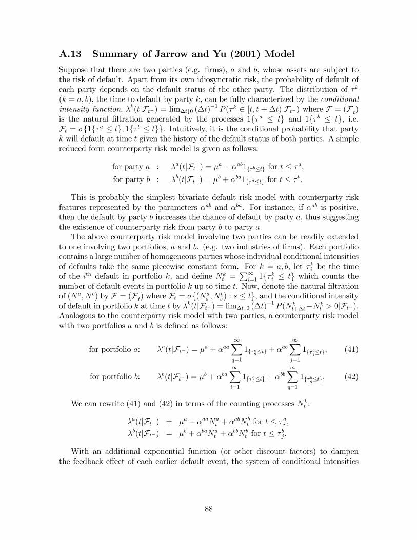
A.13 Summary of Jarrow and Yu (2001) Model

Suppose that there are two parties (e.g. �rms), a and b, whose assets are subject tothe risk of default. Apart from its own idiosyncratic risk, the probability of default ofeach party depends on the default status of the other party. The distribution of � k

(k = a; b), the time to default by party k, can be fully characterized by the conditionalintensity function, �k(tjFt�) = lim�t#0 (�t)

�1 P (� k 2 [t; t + �t)jFt�) where F = (F t)is the natural �ltration generated by the processes 1f�a � tg and 1f� b � tg, i.e.Ft = �f1f�a � tg; 1f� b � tgg. Intuitively, it is the conditional probability that partyk will default at time t given the history of the default status of both parties. A simplereduced form counterparty risk model is given as follows:

for party a : �a(tjFt�) = �a + �ab1f�b�tg for t � �a;for party b : �b(tjFt�) = �b + �ba1f�a�tg for t � � b:

This is probably the simplest bivariate default risk model with counterparty riskfeatures represented by the parameters �ab and �ba. For instance, if �ab is positive,then the default by party b increases the chance of default by party a, thus suggestingthe existence of counterparty risk from party b to party a.The above counterparty risk model involving two parties can be readily extended

to one involving two portfolios, a and b. (e.g. two industries of �rms). Each portfoliocontains a large number of homogeneous parties whose individual conditional intensitiesof defaults take the same piecewise constant form. For k = a; b, let � ki be the timeof the ith default in portfolio k, and de�ne Nk

t =P1

i=1 1f� ki � tg which counts thenumber of default events in portfolio k up to time t. Now, denote the natural �ltrationof (Na; N b) by F = (F t) where Ft = �f(Na

s ; Nbs ) : s � tg, and the conditional intensity

of default in portfolio k at time t by �k(tjFt�) = lim�t#0 (�t)�1 P (Nk

t+�t�Nkt > 0jFt�).

Analogous to the counterparty risk model with two parties, a counterparty risk modelwith two portfolios a and b is de�ned as follows:

for portfolio a: �a(tjFt�) = �a + �aa1Xq=1

1f�aq�tg + �ab

1Xj=1

1f�bj�tg; (41)

for portfolio b: �b(tjFt�) = �b + �ba1Xi=1

1f�ai�tg + �bb

1Xq=1

1f�bq�tg: (42)

We can rewrite (41) and (42) in terms of the counting processes Nkt :

�a(tjFt�) = �a + �aaNat + �

abN bt for t � �ai ;

�b(tjFt�) = �b + �baNat + �

bbN bt for t � � bj:

With an additional exponential function (or other discount factors) to dampenthe feedback e¤ect of each earlier default event, the system of conditional intensities

88

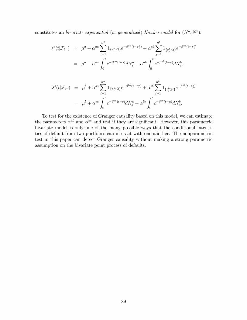
constitutes an bivariate exponential (or generalized) Hawkes model for (Na; N b):

�a(tjFt�) = �a + �aanaXi=1

1f�ai�tge��aa(t��ai ) + �ab

nbXj=1

1f�bj�tge��ab(t��bj)

= �a + �aaZ t

0

e��aa(t�s)dNa

s + �ab

Z t

0

e��ab(t�u)dN b

u;

�b(tjFt�) = �b + �banaXi=1

1f�ai�tge��ba(t��ai ) + �bb

nbXj=1

1f�bj�tge��bb(t��bj)

= �b + �baZ t

0

e��ba(t�s)dNa

s + �bb

Z t

0

e��bb(t�u)dN b

u:

To test for the existence of Granger causality based on this model, we can estimatethe parameters �ab and �ba and test if they are signi�cant. However, this parametricbivariate model is only one of the many possible ways that the conditional intensi-ties of default from two portfolios can interact with one another. The nonparametrictest in this paper can detect Granger causality without making a strong parametricassumption on the bivariate point process of defaults.

89