Granger Causality and Dynamic StructuralSystems

Halbert White and Xun LuDepartment of Economics, UCSD

October 15, 2008

Objective

Relate Granger causality to a notion of structural causality

� Granger (G) causality

(Granger, 1969 and Granger and Newbold, 1986)

� Structural causality

(White and Chalak, 2007 and White and Kennedy, 2008)

Outline

1. De�ne G non-causality and structural non-causality

2. Relation between (retrospective, weak) G non-causality andstructural non-causality

3. Testing (retrospective) weak G non-causality

4. Testing (retrospective) conditional exogeneity andstructural non-causality

5. Applications

6. Conclusions

1. De�nitions of G non-causality and structuralnon-causality

Granger Causality

� Let N0 := f0, 1, 2, 3...g and N := f1, 2, 3...g.� subscriptt denotes a variable at time t.� superscriptt denotes a variable�s "t-history",(e.g., X t = fX0,X1, ...,Xtg)

De�nition: Granger non-causalityLet fDt ,St ,Ytg be a sequence of random vectors. Suppose that

Yt+1 ? Dt j Y t ,S t for all t 2 N0

then we say D does not G -cause Y with respect to S .Otherwise, we say D G -causes Y with respect to S .

Data Generating Process (DGP)

Assumption A.1(a) (White and Kennedy, 2008) LetV0,W0,D0,Y0 be random vectors and let fZtg be a stochasticprocess. fVt ,Wt ,Dt ,Ytg is generated by the structural equations

Vt+1 = b0,t+1(V t ,Z t )Wt+1 = b1,t+1(W t ,V t ,Z t )Dt+1 = b2,t+1(Dt ,W t ,V t ,Z t )Yt+1 = qt+1(Y t ,Dt ,V t ,Z t ) t = 0, 1, 2...

� Cause of interest: Dt . Response of interest: Yt+1.� fDt ,Yt ,Wtg observable; some components of fZt ,Vtgunobservable

� Covariates: Xt := fWt , observable components of Zt and Vtg� Unobservables: Ut� b0,t+1, b1,t+1, b2,t+1, qt+1 unknown functions.

Alternative Data Generating Process (DGP)

Assumption A.1(a) (White and Kennedy, 2008) LetV0,W0,D0,Y0 be random vectors and let fZtg be a stochasticprocess. fVt ,Wt ,Dt ,Ytg is generated by the structural equations

Vt+1 = b0,t+1(V t ,Z t+1)Wt+1 = b1,t+1(W t ,V t+1,Z t+1)Dt+1 = b2,t+1(Dt ,W t+1,V t+1,Z t+1)Yt+1 = qt+1(Y t ,Dt+1,V t+1,Z t+1) t = 0, 1, 2...

Structural Causality

� Implicit dynamic representation of the DGP:

Yt+1 = rt+1(Y0,Dt ,V t ,Z t ) t = 0, 1, 2, ...

� De�nition: Structural non-causality

Suppose for given t and all y0, v t , and z t , the function

d t ! rt+1(y0, d t , v t , z t )

is constant in d t . Then we say Dt does not structurally causeYt+1 and write Dt 6)S Yt+1. Otherwise, we say Dt structurallycauses Yt+1 and write Dt )S Yt+1.

� Example: Yt+1 = β0 + Y0β1 +Dt 0β2 + V

t 0β3 + Zt 0β4

β2 = 0: structural non-causalityβ2 6= 0: structural causality

2. Relation between G non-causality and structuralnon-causality

Weak Granger Causality

� De�nition: Weak G non-causality

Let fDt ,St ,Ytg be a sequence of random vectors. Suppose that

Yt+1 ? Dt j Y0,S t for all t 2 N0

then we say D does not weakly G -cause Y with respect to S .Otherwise, we say D weakly G -causes Y with respect to S .

Note: G non-causality says Yt+1 ? Dt j Y t ,S t for all t 2 N0

Conditional Exogeneity

� Assumption A.2 (a)

Dt ? U t j Y0,X t , t = 0, 1, 2, ... .

We say Dt is conditionally exogenous with respect to U t given(Y0,X t ), t = 0, 1, 2, ... . For brevity, we just say Dt isconditionally exogenous.

Structural Non-causality and (Weak) G Non-causality

� Proposition 1

Suppose Assumption A.1(a) holds and that Dt 6)S Yt+1 for allt 2 N0. If Assumption A.2(a) also holds, then D does not(weakly) G�cause Y with respect to X .

� Structural non-causality and conditional exogeneity imply(weak) G non-causality

Retrospective Weak Granger Causality

� Time line

� De�nition: Retrospective weak G non-causality

Let fDt ,St ,Ytg be a sequence of random variables. For a givenT 2 N, suppose that

Yt+1 ? Dt jY0,ST for all 0 � t � T � 1

Then we say D does not retrospectively weakly G -cause Y withrespect to S . Otherwise, we say D retrospectively weaklyG -causes Y with respect to S .

Retrospective Conditional Exogeneity

� Assumption A.2 (b)

Dt ? U t j Y0,XT , t = 0, 1, 2, ... .

We say Dt is retrospectively conditionally exogenous with respectto U t given (Y0,XT ), t = 0, 1, 2, ... . For brevity, we just say Dt isretrospectively conditionally exogenous.

Structural Non-causality and Retrospective (Weak) GNon-causality

� Proposition 2

Suppose Assumption A.1(a) holds and that Dt 6)S Yt+1 for allt 2 N0. If Assumption A.2(b) also holds, then for the given T , Ddoes not retrospectively (weakly) G cause Y with respect to X .

� Structural non-causality and retrospective conditionalexogeneity imply retrospective (weak) G non-causality

Some Converse Results

� Assumption A.3(a) there exist measurable sets BY ,B0,BD ,and BX such that:

(i)P [Yt+1 2 BY ,Y0 2 B0,Dt 2 BD ,X t 2 BX ] > 0

(ii)P [Dt 2 BD jY0 2 B0,X t 2 BX ] < 1; and

(iii) with

BU (dt , y0, x t ) � supp(U t j Dt = d t ,Y0 = y0,X t = x t ),

for all d t /2 BD , y0 2 B0, and x t 2 BX , and all ut 2 BU (d t , y0, x t )

rt+1(y0, d t , v t , z t ) 62 BY .

Some Converse Results (Cont�d)

� Intuition of A.3(a)

� Example of A.3(a):

Yt+1 = Dt + Ut , Dt � N (0, 1) , Ut �Uniform(0, 1) ;BD = (�∞, 0) [ (1,∞) and BY = (�∞, 0) [ (2,∞).dt /2 BD means dt 2 [0, 1]. For all dt 2 [0, 1] and ut 2 (0, 1) ,yt+1 = dt + ut 2 (0, 2), which is not contained in BY .

Some Converse Results (Cont�d)

� De�nition: Strong Causality

Suppose A.1(a) and A.3(a) hold. Then we say that Dt stronglycauses Yt+1. Otherwise, we say that Dt does not strongly causeYt+1.

� Proposition 3

If Dt strongly causes Yt+1 for all t, then D weakly G -causes Ywith respect to X .

Some Converse Results (Cont�d)

� Similarly, we can de�ne Retrospective Strong Causality byreplacing X t with XT in A.3(a).

� Proposition 4

If Dt retrospectively strongly causes Yt+1, then D retrospectivelyweakly G -causes Y with respect to X .

Summary of the relation between (retrospective) weak Gcausality and structural causality

� Under (retrospective) conditional exogeneity, structuralnon-causality implies (retrospective) weak G non-causality.

Conversely,

� (Retrospective) strong causality implies (retrospective) weakG causality.

3. Testing (retrospective) weak G non-causality

Testing (Retrospective) Weak G Non-causality

� Weak G non-causality:

Yt+1 ? Dt jY0,X t

� (Retrospective) weak G non-causality:

Yt+1 ? Dt jY0,XT

Testing (Retrospective) Weak G Non-causality (Cont�d)

� Proposition 5

(a) Under some conditional stationarity and memory assumptions,then

Yt+1 ? Dt j Y0,X t , Yt+1 ? Dt j Yt ,X tt�τ

Notation: X tt�τ := (Xt�τ,Xt�τ+1, ...,Xt )

(b) Under some conditional stationarity and memory assumptions,then

Yt+1 ? Dt j Y0,XT , Yt+1 ? Dt j Yt ,X t+τt�τ

Notation: X t+τt�τ := (Xt�τ,Xt�τ+1, ...,Xt ,Xt+1,Xt+2,...,Xt+τ)

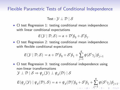
Flexible Parametric Tests of Conditional Independence

Test : Y ? D j S� CI test Regression 1: testing conditional mean independencewith linear conditional expectations

E (Y j D,S) = α+D0β0 + S 0β1.� CI test Regression 2: testing conditional mean independencewith �exible conditional expectations

E (Y j D,S) = α+D0β0 + S 0β1 +q

∑j=1

ψ(S 0γj )βj+1

� CI test Regression 3: testing conditional independence usingnon-linear transformationsY ? D j S ) ψy (Y) ? ψd (D) j S

E (ψy (Y) j ψd (D),S) = α+ ψd (D)0β0 + S 0β1 +q

∑j=1

ψ(S 0γj )βj+1.

4. Testing (retrospective) conditional exogeneity

(Retrospective) Conditional Exogeneity

� Conditional exogeneity:

U t ? Dt jY0,X t

� Retrospective conditional exogeneity:

U t ? Dt jY0,XT

Challenge: Ut is unobservable.

Resolution: Observe additional proxies for Ut , say Wt �can useWt to test (retrospective) conditional exogeneity.

Testing Conditional Exogeneity

� Assumption A.6 (a) W0 is an observable random variableand fUtg is an unobservable stochastic process such that (i)fWtg is generated by the structural equations

Wt+1 = b3,t+1(W t ,X t ,U t , U t ), t = 0, 1, ...,

where b3,t+1 is an unknown measurable function; and (ii)

Dt ? (U t , W0) j Y0,U t ,X t , t = 1, 2, ... .

� Assumption A.7 (a) (Wt+1, Wt ) ? (W0,Y0) j X t for allt = 1, 2, ... .

Testing Conditional Exogeneity (Cont�d)

� Proposition 6

Suppose Assumptions A.1(a), A.6(a), and A.7(a) hold. ThenDt ? U t j Y0,X t for all t 2 N implies Wt+1 ? Dt j W0,X t for allt 2 N0.

� Proposition 7

Under some conditional stationarity and memory assumptions,

Wt+1 ? Dt jW0,X t for all t 2 N0

, Wt+1 ? Dt j Wt ,X tt�τ for all t 2 N0

� Similarly, test Retrospective Conditional Exogeneity byreplacing X t ,X tt�τ with X

T ,X t+τt�τ .

A Pure Test of Structural Non-causality

Reject structural non-causality if

� the (retrospective) (weak) G non-causality test rejects; and� the (retrospective) conditional exogeneity test fails to reject.

Signi�cance Level and Power of the StructuralNon-causality Test

� Test levelsα1 : conditional exogeneity testα2 : G non-causality testα : structural non-causality test

� Test powersπ1 : conditional exogeneity testπ2 : G non-causality testπ : structural non-causality test

Proposition 8

max f0,min f(α2 � α1) , (π2 � π1) , (α2 � π1)gg �α � maxfminf1� α1, α2g,minf1� π1,π2g,minf1� π1, α2gg

π2 � α1 � π � min f1� α1,π2g .

Signi�cance Level and Power of the StructuralNon-causality Test (Cont�d)

� Test levelsα1T ! α1 : conditional exogeneity testα2T ! α2 : G non-causality testαT : structural non-causality test

� Test powersπ1T ! 1 : conditional exogeneity testπ2T ! 1 : G non-causality testπT : structural non-causality test

Proposition 9

0 � lim inf αT � lim sup αT � minf1� α1, α2g and

πT ! 1� α1.

5. Applications

Applications

� Crude oil prices and gasoline prices (White and Kennedy,2008)

� Monetary policy and industrial production (Angrist andKuersteiner, 2004)

� Economic announcements and stock returns (Flannery andProtopapadakis, 2002)

Crude Oil Prices and Gasoline Prices

� Yt : the natural logarithm of the spot price for US Gulf Coastconventional gasoline

� Dt : the natural logarithm of the Cushing OK WTI spot crudeoil price

� Ut : all unobservable drivers of gasoline prices� Structure:

Yt = rt (Y0,Dt ,U t ), t = 0, 1, ...,T .

� Note: "Contemporaneous" e¤ects allowed.� Sample period: January 1987-December 1997

Crude Oil Prices and Gasoline Prices (Cont�d)

� Xt = Wt :

(1) natural logarithm of Texas Initial and ContinuingUnemployment Claims

(2) Houston temperature(3) winter dummy for January, February, and March(4) summer dummy for June, July, and August(5) natural logarithm of U.S. Bureau of Labor Statistics

Electricity price index(6) 10-Year Treasury Note Constant Maturity Rate(7) 3-Month T-Bill Secondary Market Rate(8) Index of the Foreign Exchange Value of the Dollar

� Wt : natural logarithm of the U.S. Bureau of Labor StatisticsNatural Gas Price Index.

Crude Oil Prices and Gasoline Prices (Cont�d)

� Test retrospective conditional exogeneity by testing

Dt ? Wt j Wt�1,X t+τt�τ (1)

� Test retrospective weak G non-causality by testing

Yt ? Dt j Yt�1,X t+τt�τ (2)

� Results:

1. Fail to reject (1) using CI test Regressions 1, 2, 3 foralmost all the choices of τ (τ = 0, 1, ..., 5) and q (q = 1, 2, ..., 5) .

2. Reject (2) using CI test Regressions 1, 2, 3 for almost allthe choices of τ (τ = 0, 1, ..., 5) and q (q = 1, 2, ..., 5) .

Crude Oil Prices and Gasoline Prices (Cont�d)

� Conclusions: reject the hypothesis of structural non-causalityfrom crude oil prices to gasoline prices.

� Similar conclusions using non-retrospective conditionalexogeneity and weak G non-causality tests.

� Conclusions not surprising �But they critically supportsubsequent inferences about e¤ect magnitudes.

Conclusions

This paper

� Links G non-causality and a notion of structural non-causality� Provides explicit guidance as to how to choose S so Gnon-causality gives structural insight

� Extends G non-causality to new weak and retrospective weakversions

� Provides new tests of (retrospective) weak G non-causality,(retrospective) conditional exogeneity, and structuralnon-causality