a nonlinear quantile regression test of the pecking order model
TRANSCRIPT
1
A Nonlinear Quantile Regression Test of the Pecking Order Model
Jiaping Qiu*,
DeGroote School of Business, McMaster University, 1280 Main Street West, Hamilton, Ontario, Canada L5S 4M4
Brian F. Smith
Clarica Financial Services Research Centre, School of Business and Economics, Wilfrid Laurier University, Ontario, Canada, N2L 3C5
Abstract
Past empirical tests on the pecking order model by Shyam-Sunder and Myers (1999) and Frank and Goyal (2003a) draw sharply different findings on the financial deficit-net debt issue relationship. This paper presents a nonlinear quantile regression test which accounts for nonlinearities in the internal financial deficit-net debt relationship and captures the distribution of the net debt issue conditional on financial deficits. We find that when the internal financial deficit is below 10% of total assets, almost all companies use debt to cover the deficit. When financial deficits exceed 30% of total assets, most companies choose equity financing. However, when financial surpluses are generated, most companies use those surpluses to repay debt independent of the size of the surplus. Our finding shows that the different findings in Shyam-Sunder and Myers (1999) and Frank and Goyal (2003a) are in fact consistent after accounting for the nonlinearity.
* Qiu is the contacting author and can be contacted at the DeGroote School of Business, McMaster University, 1280 Main Street West, Hamilton, Ontario, Canada L5S 4M4. Phone: 905-515-9140 ext. 23963. Fax: 905-521-8995. E-mail: [email protected]. We would like to thank seminar participants at the McMaster University and Northern Finance Association 2005 meeting. We are grateful to the financial support from the SSHRC and the CMA center at Wilfrid Laurier University.

2
A Nonlinear Quantile Regression Test of the Pecking Order Model
Abstract
Past empirical tests on the pecking order model by Shyam-Sunder and Myers (1999) and Frank and Goyal (2003a) draw sharply different findings on the financial deficit-net debt issue relationship. This paper presents a nonlinear quantile regression test which accounts for nonlinearities in the internal financial deficit-net debt relationship and captures the distribution of the net debt issue conditional on financial deficits. We find that when the internal financial deficit is below 10% of total assets, almost all companies use debt to cover the deficit. When financial deficits exceed 30% of total assets, most companies choose equity financing. However, when financial surpluses are generated, most companies use those surpluses to repay debt independent of the size of the surplus. Our finding shows that the different findings in Shyam-Sunder and Myers (1999) and Frank and Goyal (2003a) are in fact consistent after accounting for the nonlinearity.

3
1. Introduction
The finance literature offers two main competing models to explain the financing decisions of
companies. The tradeoff model asserts that companies find an optimal capital structure by
weighing the marginal costs against the benefits of additional debt. In particular, the potential
bankruptcy and agency costs of increased debt are compared with the income tax savings from
interest deductibility and the reduction of free-cash flow agency problems. The pecking order
model developed by Myers (1984) and Myers and Majluf (1984) asserts that companies are
reluctant to issue risky securities because of transactions costs as well as the costs associated with
information asymmetry between management and potential investors about the securities’ value.
When they need financing, companies prefer to use internal sources, then debt and finally equity.
The modified pecking order model incorporates financial distress costs. That is, when the marginal
costs of debt are very high as would occur when companies are highly levered, equity is most
likely issued.
Shyam-Sunder and Myers (1999, hereinafter, SSM) propose an empirical test of the
pecking order model that relates changes in the amount of debt issued to the internal cash flow
deficit. In a regression of net debt issues on the financing deficit using a sample of 157 firms that
had traded continuously over the period 1971 to 1989, SSM find the slope coefficient is close to
one. They argue that the results support the prediction of pecking order theory that firms tend to
fund financial deficits by issuing debt. A study by Frank and Goyal (2003a, hereinafter, FG) finds
that the SSM test lacks robustness when applied to a much larger sample of companies over a
longer period of time and when conventional leverage factors are included. FG find that contrary
to the pecking order model, net equity issues track the financial deficit better than net debt issues.
Chirinko and Singha (2000), however, raise two concerns about the empirical models used by

4
SSM and FG: first, unless it equals one, the estimated coefficient on net debt issue from an OLS
regression of net debt issue on financial deficit can not be used to differentiate the modified
pecking order model from the static trade-off model. For example, a coefficient of 0.8 may arise
because four fifths of companies issue only debt to meet a deficit while the other fifth, who have
exhausted their ability to issue debt, issue only equity. Alternatively, a coefficient of 0.8 may arise
because all firms regularly issue a four to one mix of debt and equity to maintain an optimal
leverage ratio of 0.8. Second, the relationship between debt issue and financial deficit is expected
to be conditional on the size of the deficit. In particular, highly indebted companies face greater
than normal expected bankruptcy costs and thus are more likely to choose equity. As a result, the
relationship between net debt issue and financial deficit is likely to be nonlinear.
The purpose of this paper is to provide a new empirical test which accounts for FG’s
criticism and offer an explanation for the seemingly conflicting results by SSM and FG.
Specifically, we adopt a piece-wise linear model to capture nonlinearities in the relationship
between the internal financial deficit and the net debt issues of companies. Moreover we estimate
the piece-wise linear model using quantile regression. Quantile regression offers two important
advantages over mean regression (e.g., OLS). First, median regression (a special case of quantile
regression) is robust to outliers. Moreover, we show later that the distribution of net debt issue is
highly skewed and, as a result, compared to the mean, the median is a better representative of
sample central tendency. Second, by estimating the effect of financial deficit on different quantiles
of net debt issue, quantile regression allows us to capture the whole distribution of net debt issues
conditional on the financial deficit. This is especially important since it allows us to identify the
proportion of firms that do not use net debt issues to cover financial deficits conditional on a given
level of financial deficits.
5
We estimate the net debt issue – financial deficit relationship on two samples selected by
the criteria of FG and SSM respectively, using the piece-wise linear quantile regression approach.
Consistent with Chirinko and Singha (2000), we find that the net debt issue – financial deficit
relationship is highly nonlinear. Specifically, when the financial deficit is less than 20% of assets,
most firms use debt to fund the deficit. When the financial deficit is larger than 20% of assets,
most firms issue some equity. In contrast to the response to internal financial deficits, we find that
financial surpluses are generally used to repay debt regardless of the size of the surplus. We also
find that conventional leverage factors such as firm size, profitability, market to book values and
tangibility affect a company’s response to financial deficits and surpluses.
We provide an explanation for the different findings by SSM and FG. The key difference
between SSM and FG’s samples is that the former includes firms with relatively low financial
deficit (with a maximum financial deficit-to-total asset ratio of 0.37) while the latter includes firms
with large financial deficit (with a maximum financial deficit-to total asset ratio of 0.999). We
apply piece-wise linear quantile regression to the FG sample and find that when the financial
deficit is below 0.30, the relationship is consistent with SSM. When the financial deficit is above
0.3, the relationship is flatter and when the deficit is above 0.5, the relationship is completely flat.
Thus, FG’s finding of a flatter relationship between financial deficit and net debt is due to 1) a
subset of firms with high financial deficit that are in FFG’s sample but not SSM’s and 2) a
misspecification of the linear model.
The paper is organized as follows. Section 2 describes the methodology used in this paper
Section 3 discusses the data. Section 4 presents the empirical results on the sample of Shyam-
Sunder and Myers (1999) using nonlinear quantile regression. Section 5 explains the reasons for
the different findings of SSM and FG. Section 6 summarizes and concludes the paper.
6
2. Methodology
SSM and FG test the relationship between firm’s debt issue and financial deficits with the
following regression model:
tititi bDeficitaDebt ,,, ε++=∆ (1)
where ∆Debti,t is the net debt issue of firm i at time t. Deficiti,t is the financial deficit of firm i at
time t. Financial deficit is defined as the sum of dividends, investments and the change of working
capital minus internal cash flow. Equation (1) provides a parsimonious way to test the relationship
between net debt issue and financial deficit. As Chirinko and Singha (1999) discuss, however,
under the null hypothesis of a modified pecking order model, the relationship between net debt
issues and financial deficits should be nonlinear. That is, when the deficit is so high that it could
trigger financial distress, firms will issue equity instead of issuing debt.
To address the potential nonlinearity in the net debt issue-financial deficit relationship, we
employ a piece-wise linear regression which allows for the effect of financial deficits on debt issue
to depend on the size of financial deficits. For our purpose, piece-wise linear specification is
preferable to nonlinear specifications such as quadratic and logarithm functions. Piece-wise linear
specification provides a more flexible function form which allows us to test whether and to what
extent there is a one to one relationship between net debt issue and financial deficit. In contrast,
quadratic and logarithm functions can only test whether or not the net debt issue – financial deficit
relationship is concave or convex. Testing a one to one relationship between net debt issue and
financial deficit is especially important since it is the key predication of pecking order theory.
In addition to nonlinearity, the highly skewed distributions of net debt issues suggest the
coefficients estimated from the mean regression (OLS) in past studies may not be a sufficient
description of distribution of net debt issue conditional on financial deficit. We estimate the piece-

7
wise linear model using quantile regression as it offers two potential benefits over least squares.
First, it is more robust to both outliers and deviations from normality. In other words, even if one
is solely interested in a measure of central tendency, estimates of the conditional median, which
minimize the sum of absolute errors, are less sensitive to outliers than estimates of the conditional
mean, which minimize the sum of squared errors. This robustness property is important to the
current study, since net debt issue is highly skewed. Most importantly for our study, quantile
regression offers a richer description of the manner in which the regressors influence the
dependent variable. Rather than restricting the influence of financial deficits to shifts in the
conditional mean of net debt issue, it allows for differential effects of financial deficit at different
points in the distribution of net debt issue. This is especially useful for our purpose because it
allows us to identify the proportion of firms that do not use net debt issues to cover financial
deficits conditional on a given level of financial deficits.
Just as regression estimates the expectation of the dependent variable Y , conditional on the
regressors X, the quantile regression, introduced by Koenker and Bassett (1978), estimates the
quantile, )|( xQY τ , of Y , conditional on xX = , where )1,0(∈τ indexes the quantile level and
where capital letters denote random variables and lower case letters denote their realizations. In a
linear quantile regression model this is specified as
).()|( τγτ xxQY ′=
In the regression case, the conditional expectation minimizes the expected quadratic loss in
predicting Y conditional on X . This leads naturally to the ordinary least squares estimator, in
which the regression coefficient β)
is chosen to minimizes the sample analogue
∑ ′−=
n
iii XY
n 1
2)(1 β
8
with respect to β . Likewise, Koenker and Bassett (1978) show that if the quadratic loss function
is replaced by the asymmetric absolute deviation loss function,
))0(1()( <−= uuu τρτ
then the expected loss is instead minimized by the conditional quantile )|( xQY τ . As in OLS, the
quantile regression coefficients are then chosen to minimize the finite sample analogue. In other
words, the τ quantile regression coefficient )(τγ) minimizes
∑ ′−=
n
iii XY
n 1)(1 γρτ
with respect to γ . For example, ||2/1)( uu =τρ is used for Laplace’s median regression function.
3. Sample Constructions
The data is from the Compustat annual file (including P/S/T, Full Coverage and Research files).
Since American firms started reporting funds flow statements from 1971, our sample period begins
in 1971. It ends in 2001. Following the tradition in capital structure literature, we delete financial
firms (SIC codes 6000-6999) and regulated utilities firms (SIC 4900-4999), firms involved in
major mergers (COMPUSTAT footnote code AB) and firms that reported format code 4, 5 or 6.
The sample in SSM includes only firms with data on cash flow reported annually for all
years from 1971 to 1989. FG re-investigate SSM’s test using a larger sample which includes firms
from the year 1971 to 1998 without the restriction of continuous observations. In order to
understand whether data selection plays a role in the different conclusions drawn in the SSM and
FG tests, we construct two samples. One attempts to match the sample selection criteria by SSM
which requires that firms report their deficit and net debt issues without break over the period 1971
to 1989. These criteria result in a sample with 808 firms each with 19 years of data. The other
sample attempts to match the sample selection criteria by FG which includes all firms in the

9
Compustat dataset from 1971 to 2001. To avoid the effect of outliers in the data, we remove the
top and bottom 1% observations of the variables used in both samples and observations with
deficits to assets ratio greater than one. The details of how the variables are constructed from the
Compustat database are provided in the Appendix.
Table 1 compares the summary statistics in the sample with continuous observations from
1971 to 1989 and those in the unrestricted full sample. Inspection of Panel A in Table 1 reveals
that sample firms with continuous observations between years 1971 to 1989 are older and larger
than those in the full sample. In addition, the sample firms with continuous observations have
more tangible assets and are more profitable than those in the full sample. Most critically for tests
of capital structure, firms in the sample with continuous observations have much smaller financial
deficits than firms in the unrestricted sample. The average deficit to assets ratio is 0.017 in the
sample with continuous observations, which is nearly one quarter of the corresponding number in
the unrestricted sample (0.061). Yet the average net debt issues to assets ratios across the two
samples are both 0.013. The unrestricted sample uses much larger net equity issues (on average,
0.048 vs. 0.004) to offset the larger internal deficit. Given the large differences in the size of the
financing deficit, in the use of equity and in other fundamental characteristics of the companies
selected by SSM and FG, it is not surprising their conclusions differ.
Panel B summarizes the distributions of financial deficits, net debt issues and net equity
issues. Consistent with its higher mean, the maximum financial deficit of firms in the full sample
is 0.999 versus 0.368 for the sample with continuous observations while the minimum financial
deficits do not greatly differ between the two samples (-0.344 versus -0.238). This finding
suggests an asymmetry in the size of financial surpluses versus deficits. The distribution of net
debt issues has a skewness greater than 1 and a kurtosis greater than 6, both in the sample with
10
continuous observations and in the full sample. Similar patterns are observed for the distribution of
financial deficits and net equity issues.
Figure 1 shows the distribution of financial deficits of the two samples. For both samples,
80% of observations have a deficit to asset ratio less than 0.2. Yet, the sample of all firms has
more observations with large financial deficits. This is consistent with the fact that firms with
continuous observation from year 1971 to 1989 are larger and more mature than firms in the full
sample. They are less likely to have large financial deficits. Even though the proportion of firms
having large financial deficits is quite small, as we will show later, it is important in the empirical
test to capture the debt issuing behavior of this group of firms because they may behave quite
differently from firms with relatively low financial deficit, according to the prediction of the
modified pecking order theory.
4. Results
We first apply our methods to examine the sample matching the selection criteria by SSM, that is,
the sample with continuous observations from 1971 to 1989. Since the maximum financial deficit
in this sample is 0.37, we subdivide the range of positive financial deficits into three bands and
create three explanatory variables to capture the nonlinear effect of financial deficits on debt
issues:1
)1.0 to0.0(,tiDeficit 1.0
,
=
= tideficit
;10 100
.deficitif ,.deficit if
i,t
i,t
≥
≤≤
)2.0 to1.0(,tiDeficit
..-deficit i,t
1010
0
=
==
;. deficitif
,.deficit.if.deficitif
i,t
i,t
i,t
20 2010
10
≥
≤≤
≤
1 The results are robust to a wide variety of different range specifications.

11
)0.37 to0.2(,tiDeficit 0.2-
0
,tideficit==
200.37
20 .deficitif
.deficitif
i,t
i,t
≥≥
≤
For example, when the financial deficit is equal to 0.25, we would have Deficiti,t (0.0 to 0.1) equal
to 0.1, Deficiti,t (0.1 to 0.2) equal to 0.1 and Deficiti,t (0.2 to 0.37) equal to 0.05. Thus the basic
piecewise linear regression we estimate is as following,
i,ti,t
i,ti,tti
ε). to .( Deficitb) . to .(Deficitb). to .(DeficitbaDebt
+×+
×++=∆
3702020101000
3
21, (2)
The estimated coefficients of b1 to b3 will indicate the marginal effect of financial deficit changes
on net debt issues in different deficit ranges.
The static trade-off model asserts that a firm makes financing decisions based on the
optimal capital structure which is determined by a firm’s characteristics. Hovakimian, Oper and
Titman (1999) incorporate adjustment cost into the state-off model. Using a dynamic target
adjustment model, they show that net debt issue is determined by a firm’s characteristics that
explain the target leverage ratio. To incorporate the trade-off model in our tests, we follow
Hovakimian, Oper and Titman (1999) and expand equations (1) and (2) by including four more
explanatory variables that have been consistently shown in the literature to significantly affect
firms’ leverage ratio. These variables are firm size, profitability, market to book ratio and
tangibility. Thus, the expanded regressions of Equations (1) and (2) are as follows:
i,ti,ti,t
1i,ti,ti,ti,t
εyTangibilitcMTBcityProfitabilcLog(Sale)cDeficitba∆Debt
+++
+++=
−−
−−
1413
2111 (3)
i,ti,ti,t1i,ti,t
i,ti,ti,ti,t
εyTangibilitcMTBcityProfitabilcLog(Sale)c)to.(Deficitb). to .(Deficitb). to .(Deficitba∆Debt
+++++
+×++=
−−−− 1413211
321 37.0 2020101000 (4)
where Log(sale)i,t-1 equals the natural logarithm of firm i’s net sales at time t-1 and proxies for
size. Profitabilityi,t-1 equals the firm i’s net income normalized by total assets at time t-1. Market to

12
book ratio, MTBi,t-1, equals the firm i’s ratio of market value of assets (book value of assets - book
value of equity + market value of equity) divided by the book value of assets at time t-1.
Tangibilityi,t, equals firm i’s ratio of fixed to total assets at time t-1.
To provide a comparison of the results, we estimate equations (1) to (4) using both OLS
and median regressions. Table 2 presents the results on the relationship between net debt issue and
financial deficit for firms with positive financial deficits in the sample with continuous
observations from year 1971 to 1989. Column (1) in Table 2 reports the results on the simple
linear specification of Equation (1) using OLS regression as in the past studies. The coefficient on
financial deficit is 0.7153 and the adjusted R-squared is 0.58. Column (2) in Table 2 reports the
results on the expanded simple linear specification of Equation (3) using OLS regression. It
appears that the firm’s characteristics have a significant effect on its debt issue decision. However,
the inclusion of the firm’s characteristics in the regression has little effects on the net-debt issue
and financial deficit relationships. The coefficient on financial deficit is 0.7414 and the adjusted R-
squared has a small increase to 0.62. The results are similar to the findings in Shyam-Sunder and
Myers (1999) and Frank and Goyal (2003a) who report the coefficients on financial deficit to be
approximately 0.8 if the sample is restricted to firms with continuous observations from year 1971
to 1989.
However, when we move from the simple linear model to the piece-wise linear model, a
different pattern emerges. Columns (3) and (4) provide the results of the piece-wise linear OLS
regression. The coefficients of Deficiti,t(0.0 to 0.1), Deficiti,t(0.1 to 0.2) and Deficiti,t(OVER 0.2)
decrease monotonically. In the expanded piece-wise linear regressions in Column (4), the
coefficients of Deficiti,t(0.0 to 0.1), Deficiti,t(0.1 to 0.2) and Deficiti,t(OVER 0.2) are 0.8603,
0.6993 and 0.3948, respectively. The results suggest that firms tend to use debt to finance deficits
when deficits are lower. Compared to the coefficient of 0.7414 for the financial deficit variable in
13
the simple linear model in Column (2), the piece-wise results show that, without accounting for the
nonlinearity in the debt issue-financial deficit relationship, one will under-estimate the effect of
financing deficits on debt issue when financial deficits are low, but over-estimate this relationship
when financial deficits are high.
Columns (5) to (8) present the results from the median regression. In the simple linear
median regression in Column (5), the coefficient of Deficiti,t is 0.9795, which is close to a value of
one. Compared with the corresponding coefficient from the OLS regression, the coefficient from
the median regression is much larger. The difference between the results from the OLS regression
and the median regression suggests that the conditional distribution of net debt issue is non-
normal. Thus, the quantile regression is more appropriate as it is more robust to outliers and is a
better measure of central tendency.
The results from the piece-wise median regressions also indicate a nonlinear relationship
between net-debt issue and financial deficit. Column (8) shows the results from the expanded
piece-wise median regression. The coefficients on Deficiti,t(0.0 to 0.1), Deficiti,t(0.1 to 0.2) and
Deficiti,t(OVER 0.2) are 0.9975, 0.9833 and 0.2669, respectively. The non-linearity is also shown
by Figure 2. The results suggest that, when the financial deficit to assets ratio is lower than 0.2, the
median firm uses debt to cover almost all financial deficits. However, when the financial deficit is
higher than 0.2, the median firm switches to equity financing. Such a switch could be attributed to
the potential financial distress that could be engendered by a large debt issue. Thus the financing
policy of the median firm is consistent with the prediction of the modified pecking ordering model.
Another salient implication of the modified pecking ordering model is that the financial
pattern of firms with negative financial deficits (financial surplus) could be different from those of
firms with positive financial deficits. The reason is that a large financial deficit funded by a net
14
debt issue could induce financial distress, while a large financial surplus used to pay down debt
does not have such an adverse effect.
To test the impact of financial surplus on net debt issue, we estimate equations (1) to (4)
for firms with financial surplus separately. We use the following variables to estimate the
piecewise linear regressions for firms with negative financial deficits (financial surplus).
)010( to .Deficiti,t −
deficiti,t
1.0−==
;.deficitif
,deficit.-if
i,t
i,t
10 010
−≤
≤≤
). to -.-Deficit ti 24010(,
0.10
, +==
tideficit
..deficitif deficit.-if
i,t
i,t
100.24- 010 −≤≤
≤≤
For example, when the financial deficit is equal to -0.15, we would have Deficiti,t (-0.1 to
0) = -0.1, Deficiti,t (-0.24 to -0.1) = -0.05. For this test, we use fewer steps in the analysis of
financial surpluses than deficits because there are few companies with large surpluses. Table 3
reports the results on the relationship between net debt issue and financial surplus. In the expanded
piece-wise median regression, the coefficients on Deficiti,t (-0.1 to 0) and Deficiti,t (BELOW-0.1)
are 0.9999 and 0.9073, respectively. It suggests that the median firm uses almost all its financial
surplus to retire debt when the financial surplus to asset ratio is between 0 and 0.1. When the
financial surplus is higher than 0.1, the median firm starts to repurchase a small proportion of
equity.
The results from median regression only inform us about the behavior of median firms. To
provide a complete picture of the distribution of net debt issue conditional on financial deficits and
see how the asymmetry of conditional distribution of net debt issue drives the differences in results
between the median regression and OLS regression, we estimate the effect of financial deficits on
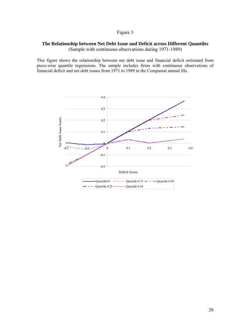
0.1, 0.25, 0.75 and 0.9 quantile net debt issues. Figure 3 concisely illustrates the relationship
between net debt issue and financial deficit from different quantile regression results. The plot

15
reveals the tendency of the dispersion of debt issues to increase along with the increase of the
firm’s financial deficit. The spacing of the quantile regression lines also reveals that the
conditional distribution of net debt issues is skewed to the right: the narrower spacing of the upper
quantiles indicates high density and a short upper tail, and the wider spacing of the lower quantiles
indicates a lower density and longer lower tail. For example, when the financial deficit to asset
ratio is below 0.1, almost all companies just use debt to offset the deficit. It is only the bottom 0.1
quantile firms that use net equity issues. When the financial deficit to asset ratio is between 0.1
and 0.2, the bottom 0.25 quantile firms use a mix of debt and equity to offset their financial
deficits. When the financial deficit to asset ratio is over 0.2, even median firms’ net debt issues are
significantly lower than the financial deficits. Furthermore, the sharpness of the kinks in the lines
in Figure 3 suggests that when companies begin to raise equity, they do so in large amounts.
Thus, the results indicate that the majority of firms use net debt issue to cover financial
deficits when the financial deficit to asset ratio is lower than 0.2. However, when financial deficits
are larger than 0.2, most of the firms start to use equity financing to cover financial deficits and
this financing comes in large blocks.
5. A Reconciliation of SSM and FG’s Results
We have shown that, once we take into account the nonlinearity in the net debt issue-financial
deficit relationship, the results on the sample of firms with continuous observations from 1971 to
1989 are largely consistent with the modified pecking order model. FG estimate a simple linear
regression on all firms in the Compustat annual file during the period of 1971 to 1998 and find that
the coefficient on financial deficit is quite low, which leads them to reject the pecking order
model. In this section, we apply piecewise linear quantile regression to the sample matching FG’s

16
sample which includes firms in the Compusat annual file from year 1971 to 2001. We compare the
results with those from the SSM sample and see if both samples provide consistent information.
As shown in the Table 1, compared with firms in the SSM sample, firms in the FG
sample have a much larger range of financial deficit. Thus we subdivide the range into ten bands
and create 10 explanatory variables, Deficiti,t (j to j+0.1), where j=0.0, 0.1, …, 0.9. The definition
of Deficiti,t (j to j+0.1) is similar to those in Equation (2). Thus, Equation (2) and (4) are modified
as follows:
∑=
++×+=∆9.0
0.0,,, )1.0j to(j
jtitijti DeficitbaDebt ε (5)
tititi
i,ttij
tijti
TangbilitycMTBc
ityProfitabilcSaleLogcDeficitbaDebt
,,4,3
2,1
9.0
0.0,, )()1.0j to(j
ε+∆×+∆×+
∆×+∆×++×+=∆ ∑= (6)
Equations (5) and (6) are identical to Equations (2) and (4) except that the latter do not include
indicator variables for financial deficit greater than 0.37, because of the lack of information in the
SSM sample. This allows us to compare the results from the SSM’s and FG’s samples for firms
with financial deficits lower than 0.37.
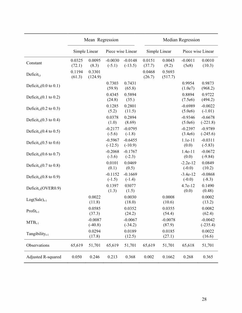
Tables 4 reports the results of estimation on Equation (1), (2), (5) and (6) using OLS and
median regression for firms with a positive financial deficit. Column (1) in Table 4 shows the
results from a simple linear regression. The coefficient on Deficit is only 0.1193 and the R2 is
0.05. In a simple linear regression including other control variables reported in Column (2) in
Table 4, the coefficient of Deficit is still quite low with a value of 0.3301, though the R2 increases
to 0.23. The results show that, in a simple linear regression, the coefficients on financial deficits
are much smaller for all firms than those with continuous observations, which is consistent with
the findings in Frank and Goyal (2003a).

17
Column (3) and (4) in Table 4 report the results from piece-wise linear regression using
OLS estimation. Columns (7) and (8) report the results using piece-wise median regression. In
each of these columns, an inspection of the coefficients on Deficiti,t(0.0 to 0.1) to Deficiti,t(0.9 to
1.0) reveals that the net-debt issue – financial deficit relationships are significantly different across
different deficit sizes. Table 5 shows the results for the firms with financial surpluses. Unlike the
results for companies with financial deficits, the nonlinearity between net-debt repurchase and
financial surplus is limited for companies with a financial surplus. The results from the expanded
piece-wise linear regression using median regression in Column (8) show that, for median firms,
there is a nearly one-to-one mapping between net-debt repurchase and financial surplus
independent of the size of the financial surplus.
Figure 4 illustrates the results in Tables 4 and 5. The piece-wise median regressions
indicate a nonlinear relationship between net-debt issue and financial deficits. It shows that, when
the deficit is below 0.2, the median firm finances nearly all its deficit by net debt issue. When
deficit to asset ratio is higher than 0.2, the median firm starts to use equity financing. The greater
is the deficit, the more equity is used by the median firm to cover the financial deficit. When the
deficit to asset ratio is higher than 0.5, the median firm uses equity to finance almost all its deficit.
In contrast, similar to the findings of Frank and Goyal (2003a), the linear OLS regression shows a
weak relationship between deficits and net debt financing.
A comparison of the results from piece-wise linear regression in Figures 2 and 4 reveals
that SSM and FG samples yield a similar net debt issue-financial deficit relationship when the
financial deficit is relatively low. That is, the median firm finances nearly all its deficit by net debt
issue when the deficit is below 0.2 and starts to use equity financing when financial deficit is
greater than 0.2. The key difference is that the SSM sample does not have observations of firms
18
with large financial deficits and is not able to capture the nonlinear relationship between net debt
issue and financial deficit when the financial deficit is relatively large.
Inspection of Figures 2 and 4 also reveals why the linear regressions obtain a larger
coefficient in SSM than in FG sample. The stronger relationship in the linear regression in the
SSM sample is due to the lack of firms with high deficit to asset ratios in their sample. In other
worlds, the flat relationship between net debt issue and financial deficit for firms with high deficits
in the FG sample reduces the slope coefficient in the linear regression. However, after accounting
for the nonlinearity and sample differences, the results of analysis of the FG and SSM samples are
consistent with each other.
6. Conclusions
This paper revisits the net debt issue – financial deficit relationship with a method that
incorporates the nonlinearities in the relationship between the internal financial deficit and the net
debt issues of companies. We employ quantile regression to accommodate non-normality and
skewness in the dependent variable, net debt issue. We find that for most companies, small internal
financial deficits (less than 10% of assets) are funded by debt whereas large internal financial
deficits (larger than 20% of assets) are funded by equity. Equity issues in the presence of large
internal deficits are consistent with the relevance of bankruptcy costs. When companies generate
financial surpluses, this nonlinearity is not present as these surpluses are used by most companies
to repay debt regardless of the size of the surplus. In summary, we reject a narrow interpretation of
the pecking order model. Rather, we find some support for a modified pecking order model that
acknowledges the primary role of bankruptcy costs in capital structure decisions when financial
deficits are large and the secondary roles of firm size, profitability, market to book values and
tangibility. The paper reconciles the conflicting findings of Shyam-Sunder and Myers (1999) and

19
Frank and Goyal (2003a). It shows that, once sample difference and nonlinearity are taken into
account, the same relationship between net debt issue and financial deficit is observed.
20
References
Chirinko, R.S., Singha, A.R., 2000. Testing static tradeoff against pecking order models of capital structure. Journal of Financial Economics 58, 417-425.
Frank, M.Z., Goyal, V.K., 2003a. Testing the pecking order theory of capital structure. Journal of
Financial Economics 67, 217-248. Frank, M.Z., Goyal, V.K., 2003b. Capital structure decisions. University of British Columbia
Working Paper. Koenker, R., Hallock, K., 2001, Quantile Regression. Journal of Economic Perspective 15, 143-
156. Myers, S.C., 1984. The capital structure puzzle. Journal of Finance 39, 575-592. Myers, S.C., Majluf, N.S., 1984. Corporate financing and investment decisions when firms have
information that investors do not have. Journal of Financial Economics 13, 187-221. Shyam-Sunder, L., Myers, S.C., 1999. Testing static tradeoff against pecking order models of
capital structure. Journal of Financial Economics 51, 219-244.

21
Table 1
Firm’s Characteristics in Different Samples
This table provides summary statistics of the samples used in this study. The full sample is from Compustat annual files 1971 to 2001, including P/S/T, Full Coverage and Research Files. The sample with continuous observations from 1971 to 1989 includes only firms that have continuous observations of net debt issues and financial deficits from 1971 to 1989. Panel A summarizes the firms’ characteristics. Firm age is the number of the years that a firm has been included in Compustat. Log(sales) is the natural logarithm of a firm’s net sales. Log(assets) is the natural logarithm of a firm’s total assets. Market to book ratio is the market value of assets (book value of assets - book value of equity + market value of equity) divided by book value of assets. Tangibility is the percentage of fixed assets in total assets. Profitability is the net income before depreciation divided by total assets. Panel B summarizes the financial deficit, net debt issue and net equity issue. Financial deficit equals (dividends + change of net working capital + investment - internal cash flow)/total assets. Net debt issue equals the new debt issue minus debt repayment. Net equity issue equals new equity issues minus equity repurchases.
Sample with continuous observations 1971-1989 Full Sample
Panel A: Firm’s Characteristics
Mean Median Std. Mean Median Std
Firm Age 29.8 30 6.54 23.83 23 10.52
Log(sales) 5.53 5.46 1.79 4.33 4.31 2.15
Log(assets) 5.21 5.07 1.81 4.27 4.13 1.98
Market to Book ratio 1.31 1.11 0.64 1.75 1.25 1.59
Tangibility 0.34 0.31 0.17 0.30 0.25 0.21
Profitability 0.16 0.15 0.08 0.10 0.13 0.23
Financial Deficit 0.017 0.0005 0.070 0.061 0.004 0.170
Net Debt Issue 0.013 0 0.062 0.013 0 0.090
Net Equity Issue 0.004 0 0.039 0.048 0 0.154
Panel B: Financial Deficit, Net Debt Issue and Net Equity Issue
Financial Deficit
Net Debt Issue
Net Equity Issue
Financial Deficit
Net Debt Issue
Net Equity Issue
Maximum 0.368 0.309 0.414 0.999 0.528 1.319
Minimum -0.238 -0.217 -0.375 -0.344 -0.378 -0.795
Skewness 1.106 1.045 1.735 2.347 1.192 3.425
Kurtosis 6.253 6.460 25.778 10.340 8.679 14.158
Observations 13,544 114,090

22
Figure 1
The Distributions of Financial Deficits
This figure shows the distributions of financial deficits in the Compustat sample of firms with continuous observations from year 1971 to 1989 and the Compustat full sample from year 1971 to 2001
a: Firms with Continuous observations from year 1971 to 1989
05
1015
20P
erce
nt
-.4 -.3 -.2 -.1 0 .1 .2 .3 .4 .5 .6 .7 .8 .9 1
Financial Deficit/Total Assets
b: All Firms from year 1971 to 2001
010
2030
Per
cent
-.4 -.3 -.2 -.1 0 .1 .2 .3 .4 .5 .6 .7 .8 .9 1
Financial Deficit/Total Assets

23
Table 2
The Relationship between Net Debt Issue and Financial Deficit for Firms with Positive Deficit
(Sample with continuous observations from 1971 to 1989) This table presents results on the net debt issue – financial deficit relationship for firms with continuous observations of financial deficit and net debt issues from 1971 to 1989 in the Compustat annual file. The analysis is restricted to observations with a non-negative financial deficit. Four regression models are used in estimations: Simple linear mean and median regressions and piece-wise linear mean and median regressions. For each type of regression, the results from two specifications are reported: The first specification includes financial deficit as the only explanatory variable. The other includes financial deficit, Log(sale), profitability, market to book ratio and tangibility as the explanatory variables. The dependent variable in the regression is firm i’s net debt issue at time t. Deficiti,t is firm i’s financial deficit at time t. Deficiti,t(0.0 to 0.1) = deficit if 0≤deficiti,t<0.1, = 0.1 if deficiti,t≥0.1; Deficiti,t (0.1 to 0.2) = 0 if 0≤deficiti,t<0.1, =deficiti,t - 0.1 if 0.1<deficiti,t<0.2, = 0.1 if deficiti,t≥0.2. Deficiti,t (OVER0.2) = 0 if 0≤deficit<0.2, =deficit-0.2 if deficit>0.2. Log(sale)i,t-1 is natural logarithm of firm i’s net sale at time t-1. Profitabilityi,t-1 is firm i’s net income normalized by total assets at time t-1. MTBi,t-1 is firm i’s market to book ratio at time t-1 as measured by (book value of assets - book value of equity + market value of equity)/book value of assets. Tangibilityi,t-1 is the firm i’s ratio of fixed assets to total assets at time t-1. t-statistics are reported in the parentheses.
Mean Regression Median Regression
Simple linear Piece wise linear Simple linear Piece wise linear
Constant 0.0033 (5.3)
0.0079 (3.8)
-0.0013 (-1.8)
0.0029 (1.4)
-0.0001 (-1.5)
0.0019 (11.9)
-0.0005 (-3.8)
0.0016 (11.7)
Deficiti,t(0.0 to 1.0) 0.7153 (100.9)
0.7414 (96.0) 0.9795
(1040.5)0.9883
(1671.5)
Deficiti,t(0.0 to 0.1) 0.8529 (55.1)
0.8603 (55.6) 0.9947
(401.1) 0.9975 (914.8)
Deficit(0.1 to 0.2) 0.6392 (25.1)
0.6993 (27.1) 0.9726
(238.7) 0.9833 (500.3)
Deficit(OVER0.2) 0.4263 (10.9)
0.3948 (9.6) 0.2771
(44.4) 0.2669 (90.9)
Log(Sale)t-1 0.0003 (1.1) 0.0004
(1.4) -0.00009 (-4.3) -0.00007
(-4.1)
Profitabilityt-1 0.0268 (4.0) 0.0296
(4.5) 0.0002 (0.4) 0.0001
(0.2)
MTBt-1 -
0.0086 (-11.2)
-0.0080 (-10.5) -0.0019
(-31.5) -0.0018 (-33.3)
Tangibilityt-1 0.0014 (0.5) -0.0008
(-0.3) 0.0007 (3.2) 0.0005
(2.6)
Observations 7,138 6,457 7,138 6,457 7,138 6,457 7,138 6,457
Adjusted R-squared 0.58 0.62 0.60 0.63 0.59 0.61 0.60 0.62

24
Table 3
The Relationship between Net Debt Issue and Financial Deficit for Firms with Negative Deficit
(Sample with continuous observations during 1971-1989)
This table presents results on the net debt issue – financial deficit relationship for firms with continuous observations of financial deficit and net debt issues from 1971 to 1989 in the Compustat annual file. The analysis is restricted to observations with a non-negative financial deficit. Four regression models are used in estimations: Simple linear mean and median regressions and piece-wise linear mean and median regressions. For each type of regression, the results from two specifications are reported: The first specification includes financial deficit as the only explanatory variable. The other specification includes financial deficit, Log(sales), profitability, market to book ratio and tangibility as the explanatory variables. The dependent variable in the regression is firm i’s net debt issue at time t. Deficiti,t is firm i’s financial deficit at time t. Deficiti,t(-0.0 to -0.1) = deficit if 0.1<deficiti,t<0, = -0.1 if deficiti,t≤-0.1; Deficiti,t (BELOW -0.1) = 0 if -0.1<deficiti,t≤0, =deficiti,t + 0.1 if deficit< -0.1. Log(sale)i,t-1 is the natural logarithm of firm i’s net sales at time t-1. Profitabilityi,t-1 is firm i’s net income normalized by total assets at time t-1. MTBi,t-1 is firm i’s market to book ratio at time t-1 as measured by (book value of assets - book value of equity + market value of equity)/book value of assets. Tangibilityi,t-1 is the firm i’s ratio of fixed assets to total assets at time t-1. t-statistics are reported in the parentheses.
Mean Regression Median Regression
Simple Linear Piece wise Linear Simple Linear Piece wise Linear
Constant -0.0021 (-1.4)
-0.0156 (-10.6)
-0.0009 (-1.8)
-0.0146 (-9.8)
-2.3e-9 (-4.1)
-0.0001 (-6.3)
-9.2e-10 (-1.7)
-3.2e-8 (-5.6)
Deficiti,t 0.6817 (71.6)
0.6524 (65.9) 0.9999
(9.0e7) 0.9951 (9.6e4)
Deficiti,t(-0.0 to -0.1) 0.7427 (53.3)
0.6958 (47.9) 0.9999
(1.5e7) 0.9999 (2.0e7)
Deficiti,t(BELOW-0.1) 0.5023 (15.9)
0.5257 (16.1) 0.9485
(3.0e7) 0.9073 (8.0e8)
Log(Sale)t-1 0.0012 (5.7) 0.0011
(5.6) 5.6e-6 (2.6) 1.9e-9
(2.4)
Profitt-1 0.0524 (10.6) 0.0517
(10.4) 0.0005 (10.0) 1.8e-7
(9.4)
MTBt-1 0.0026 (3.7) 0.0026
(3.7) -1.1e-6 (-0.15) 1.1e-9
(0.4)
Tangibilityt-1 -0.0147 (-6.4) -0.0142
(-6.2) -0.0002 (-6.7) -4.8e-8
(-5.5)
Observations 6,406 5,874 6,406 5,874 6,406 5,874 6,406 5,874
Adjusted R-squared 0.44 0.46 0.45 0.46 0.47 0.45 0.47 0.45

25
Figure 2
Summary of the Relationship between Net Debt Issue and Financial Deficit (Sample with continuous observations during 1971-1989)
This figure summarizes the relationship between net debt issue and financial deficit estimated from simple linear mean piece-wise linear median regressions in Tables 2 and 3. The sample includes firms with continuous observations of financial deficit and net debt issues from 1971 to 1989 in the Compustat annual file.
-0.2
-0.1
0
0.1
0.2
0.3
0.4
-0.2 -0.1 0 0.1 0.2 0.3 0.4
Deficit/Assets
Net
Deb
t Iss
ue/A
sset
s
Mean Regression Piece-wise Median Regression
26
Figure 3
The Relationship between Net Debt Issue and Deficit across Different Quantiles (Sample with continuous observations during 1971-1989)
This figure shows the relationship between net debt issue and financial deficit estimated from piece-wise quantile regressions. The sample includes firms with continuous observations of financial deficit and net debt issues from 1971 to 1989 in the Compustat annual file.
-0.2
-0.1
0
0.1
0.2
0.3
0.4
-0.2 -0.1 0 0.1 0.2 0.3 0.4
Deficit/Assets
Net
Deb
t Iss
ue/A
sset
s
Quantile0.9 Quantile 0.75 Quantile 0.50Quantile 0.25 Quantile 0.10
27
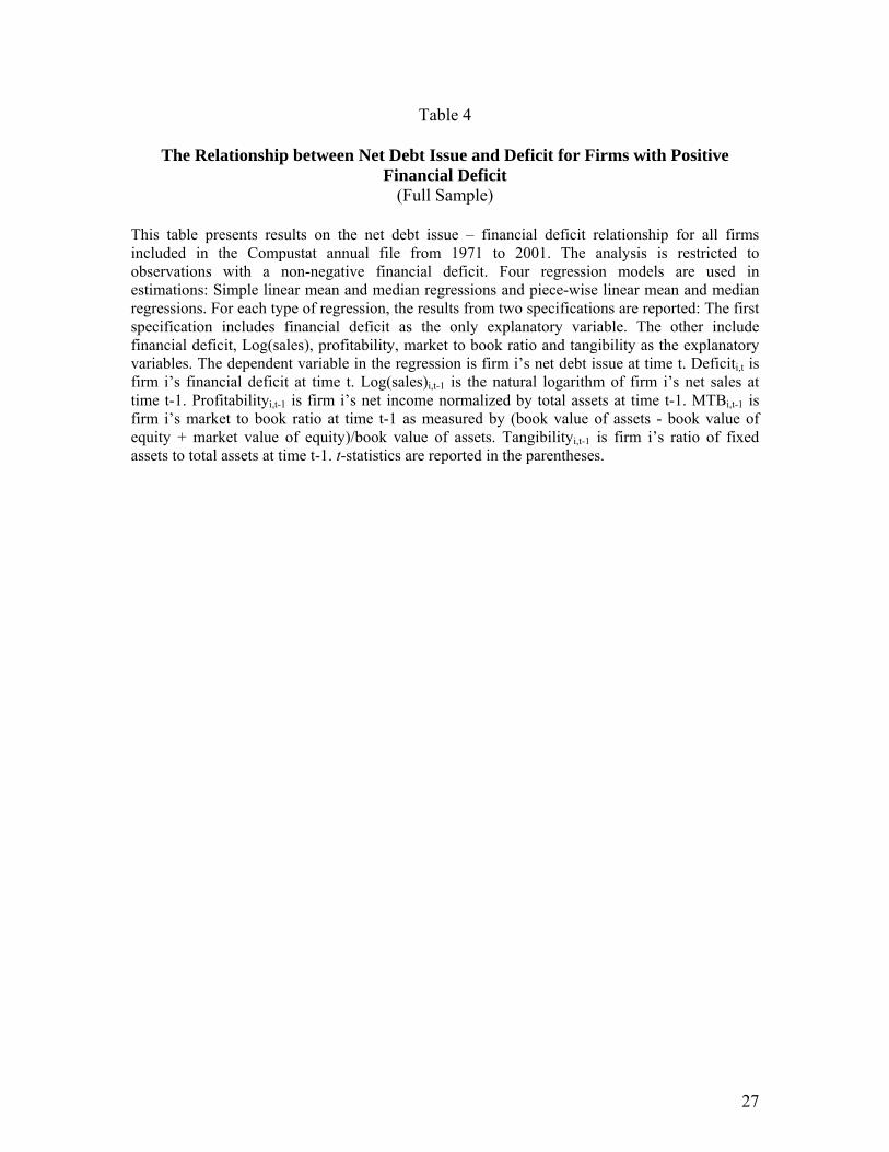
Table 4
The Relationship between Net Debt Issue and Deficit for Firms with Positive Financial Deficit
(Full Sample)
This table presents results on the net debt issue – financial deficit relationship for all firms included in the Compustat annual file from 1971 to 2001. The analysis is restricted to observations with a non-negative financial deficit. Four regression models are used in estimations: Simple linear mean and median regressions and piece-wise linear mean and median regressions. For each type of regression, the results from two specifications are reported: The first specification includes financial deficit as the only explanatory variable. The other include financial deficit, Log(sales), profitability, market to book ratio and tangibility as the explanatory variables. The dependent variable in the regression is firm i’s net debt issue at time t. Deficiti,t is firm i’s financial deficit at time t. Log(sales)i,t-1 is the natural logarithm of firm i’s net sales at time t-1. Profitabilityi,t-1 is firm i’s net income normalized by total assets at time t-1. MTBi,t-1 is firm i’s market to book ratio at time t-1 as measured by (book value of assets - book value of equity + market value of equity)/book value of assets. Tangibilityi,t-1 is firm i’s ratio of fixed assets to total assets at time t-1. t-statistics are reported in the parentheses.
28
Mean Regression Median Regression
Simple Linear Piece wise Linear Simple Linear Piece wise Linear
Constant 0.0325 (72.1)
0.0095 (8.3)
-0.0030 (-5.1)
-0.0148 (-13.5)
0.0151 (37.7)
0.0043 (9.2)
-0.0011 (5e8)
0.0010 (10.3)
Deficiti,t 0.1194 (61.3)
0.3301 (124.9) 0.0468
(26.7) 0.5693 (517.7)
Deficiti,t(0.0 to 0.1) 0.7303 (59.9)
0.7431 (65.8) 0.9954
(1.0e7) 0.9873 (968.2)
Deficiti,t(0.1 to 0.2) 0.4345 (24.8)
0.5894 (35.) 0.8894
(7.5e6) 0.9722 (494.2)
Deficiti,t(0.2 to 0.3) 0.1285 (5.2)
0.2801 (11.5) -0.6989
(5.0e6) -0.0022 (-1.01)
Deficiti,t(0.3 to 0.4) 0.0378 (1.0)
0.2894 (8.69) -0.9346
(5.0e6) -0.6678 (-221.8)
Deficiti,t(0.4 to 0.5) -0.2177 (-5.6)
-0.0795 (-1.8) -0.2397
(3.4e6) -0.9789 (-245.6)
Deficiti,t(0.5 to 0.6) -0.5967 (-12.5)
-0.6455 (-10.9) 1.1e-11
(0.0) -0.0311 (-5.83)
Deficiti,t(0.6 to 0.7) -0.2068 (-3.6)
-0.1767 (-2.3) 1.4e-11
(0.0) -0.0672 (-9.84)
Deficiti,t(0.7 to 0.8) 0.0101 (0.1)
0.0469 (0.5) -2.2e-12
(-0.0) 0.0849 (10.2)
Deficiti,t(0.8 to 0.9) -0.1152 (-1.5)
-0.1669 (-1.4) -3.4e-12
(-0.0) -0.0868 (-8.3)
Deficiti,t(OVER0.9) 0.1397 (1.3)
03077 (1.5) 4.7e-12
(0.0) 0.1490 (0.48)
Log(Sale)t-1 0.0022 (11.8) 0.0030
(18.0) 0.0008 (10.6) 0.0002
(13.2)
Profitt-1 0.0585 (37.3) 0.0352
(24.2) 0.0355 (54.4) 0.0082
(62.4)
MTBt-1 -0.0087 (-40.8) -0.0067
(-34.2) -0.0078 (87.9) -0.0042
(-235.4)
Tangibilityt-1 0.0294 (17.8) 0.0189
(12.5) 0.0185 (27.1) 0.0022
(16.6)
Observations 65,619 51,701 65,619 51,701 65,619 51,701 65,618 51,701
Adjusted R-squared 0.050 0.246 0.213 0.368 0.002 0.1662 0.268 0.365

29
Table 5
The Relationship between Net Debt Issue and Deficit for Firms with Negative Financial Deficit
(Full Sample) This table presents results on the net debt issue – financial deficit relationship for all firms included in the Compustat annual file from 1971 to 2001. The analysis is restricted to observations with a non-negative financial deficit. Four regression models are used in estimations: Simple linear mean and median regressions and piece-wise linear mean and median regressions. For each type of regression, the results from two specifications are reported: The first specification includes financial deficit as the only explanatory variable. The other include financial deficit, Log(sales), profitability, market to book ratio and tangibility as the explanatory variables. The dependent variable in the regression is firm i’s net debt issue at time t. Deficiti,t is firm i’s financial deficit at time t. Log(sales)i,t-1 is the natural logarithm of firm i’s net sales at time t-1. Profitabilityi,t-1 is firm i’s net income normalized by total assets at time t-1. MTBi,t-1 is firm i’s market to book ratio at time t-1 as measured by (book value of assets - book value of equity + market value of equity)/book value of assets. Tangibilityi,t-1 is firm i’s ratio of fixed assets to total assets at time t-1. t-statistics are reported in the parentheses.

30
Mean Regression Median Regression
Simple Linear Piece wise Linear Simple Linear Piece wise Linear
Constant -0.0018 (-8.6)
-0.0108 (-19.2)
-0.0022 (-8.7)
-0.0111 (-19.4)
1.9e-10 (1.5)
-4.1e-9 (-8.6)
-3.5e-11 (0.1)
-5.1e-10 (-9.7)
Deficiti,t 0.7619 (236.3)
0.7474 (227.0) 1.0000
(5.0e8) 1.0000 (5.0e8)
Deficiti,t(-0.0 - -0.1) 0.7485 (116.9)
0.7316 (113.1) 0.9999
(2.5e8) 0.9999 (2.4e8)
Deficiti,t(-0.1 - -0.2) 0.7656 (58.2)
0.7696 (57.5) 0.9999
(1.1e8) 0.9999 (1.1e8)
Deficiti,t(-0.2 - -0.3) 0.8084 (29.6)
0.7313 (26.2) 0.9999
(5.9e7) 0.9999 (5.0e7)
Deficiti,t(BELOW-0.3) 0.8455 (6.9)
1.0716 (8.5) 0.9999
(1.2e7) 0.9999 (1.0e7)
Log(Sale)t-1 0.0014 (16.5) 0.0015
(16.3) 4.1e-10 (5.5) 5.6e-10
(6.8)
Profitt-1 0.0258 (23.2) 0.0258
(23.2) 2.1e-8 (23.4) 2.0e-8
(20.1)
MTBt-1 0.0030 (18.5) 0.0030
(18.5) 2.7e-9 (19.6) 2.3e-9
(15.9)
Tangibilityt-1 -0.0172 (-19.6) -0.0173
(19.7) -1.0e-8 (13.6) -1.0e-8
(-12.9)
Observations 48,471 42,377 48,471 42,377 48,471 42,377 58,471 42,377
Adjusted R-squared 0.535 0.562 0.535 0.562 0.533 0.529 0.533 0.529

31
Figure 4
The Relationship between Net Debt Issue and Financial Deficit
(Full Sample)
This figure summarizes the relationship between net debt issue and financial deficit estimated from simple linear mean regressions and piece-wise linear mean and median regressions in Tables 4 and 5. The sample includes all firms in the Compustat annual file from 1971 to 2001.
-0.4
-0.3
-0.2
-0.1
0
0.1
0.2
0.3
-0.4 -0.3 -0.2 -0.1 0 0.1 0.2 0.3 0.4 0.5 0.6 0.7 0.8 0.9 1
Deficit/Assets
Net
Deb
t Iss
ue/A
sset
s
Simple Linear Mean Regression Piece-wise Linear Median Regression

32
Appendix: Measurement of Variables Variable Compustat Code Cash dividends #127
Investments For firms reporting format codes 1to 3, investments equal to #128 + #113 + #129 + #219 - #107 - #109. For firms reporting format code7, investments equal to #128 + #113 + #129 - #107 - #109 - #309 - #310.
∆ Working Capital For firms reporting format codes 1, change in net working
capital equals #236 + #274 + #301. For firms reporting format codes 2 and 3, change in net working capital equals - #236 + #274 - #301. For firms reporting format code 7, change in net working capital equals - #302 - # 303 - # 304 - #305 - #307 + #274 - #312 - # 301.
Internal cash flow For firms reporting format code 1 to 3, internal cash flow equals
#123 + #124 + #125 + #126 + #106 + #213 + #217 + #218. For firms reporting format code 7, internal cash flow equals #123 + #124 + #125 + #126 + #106 + #213 + #217 + #314.
Financial deficit Cash dividends + Investments + ∆ Working Capital - Internal
cash flow Net debt issues #111 - #114
Net equity issues #108 - #115
Log(sale) Natural Logarithm of # 12
Profitability #13/ #data6
Market to book ratio (#6-#60+#199*#54)/data6
Tangibility #7/#6