a nonlinear isogeometric finite element analysis of … nonlinear isogeometric finite element ......
TRANSCRIPT

A Nonlinear Isogeometric Finite Element Analysis of a Wind Turbine Foil
Håkon Bull Hove
Master of Science in Physics and Mathematics
Supervisor: Trond Kvamsdal, MATHCo-supervisor: Kjetil Andrè Johannessen, MATH
Department of Mathematical Sciences
Submission date: April 2014
Norwegian University of Science and Technology


......

Abstract
In the recent years, much attention has been given to the design of offshore wind turbines. To-day, the largest wind turbine has a rotor diameter of 164m. The harsh environments expose theturbines to large forces from wind and waves. During the service years of a turbine, extremewind loads must be expected. And the need for tools to accurately analyse the mechanicalproperties of the turbine blade arise.
Isogeometric analysis was introduced in [5] in 2005. One of the advantages of isogemetric anal-ysis is that we may use the same mathematical model for geometry and analysis, hence nodiscretization error occur.
With an increased size, the blades of wind turbines become relatively more flexible, and thewind load grows with the size of the blade. Peak wind loads will give large deformations. Anonlinear analysis is required for optimum results [21].
In this thesis, we have developed a static non-linear isogeometric finite element solver in Mat-lab, using bsplines as basisfuction. We started by a study of the basic properties of bsplines.We then derived the linear elasticity equation, and implemented a linear finite element code tosolve this. From this, we took the step to nonlinear analysis. We derived the weak form for theUpdated Lagrangian Formulation. This resulted in a nonlinear finite element algorithm, whichwe have implemented in Matlab.
For verification, the nonlinear isogeometric solver was compared to the isogeometric NFE pro-gram IFEM with a high level of correlation. We applied the nonlinear solver to a twisted barcase, and the wind turbine blade of the NREL offshore 5-MW baseline wind turbine.
i


Sammendrag
I de senere år har mye arbeid blitt investert i design av ofshore vinturbiner. I dag har den størsteav dem en diameter på 164 m. Belastningene fra vind og bølger vil i løpet av installasjonenslevetid kunne nå ekstremverdier. Derfor er en grundig analyse av de mekansike egenskaper idesignet påkrevd.
Isogeometrisk analyse ble introdusert i 2005 [5]. En av fordelene med denne er at den harsamme geometriske representasjon av objectet som skal analyseres som CAD programvaren.Følgelig blir det ikke diskretiseringsfeil.
Med økende bladstørrelse blir vingene mer bøyelige. Ekstrembelastninger vil gi kraftige defor-masjoner. Problemstillingen krever en ikke-lineær analyse for optimale resultater [21]
I denne avhandlingen har vi utviklet en statisk, ikke-lineær isogeometrisk finite element løseri Matlab. Denne brukes bsplines som basisfunksjoner. Vi begynte arbeidet med studier avbspline egenskapene, vi avledet så den lineære elastisitetslikningen, og implementerte an lineær"finite element" metode i Matlabkode. Ut fra denne tok vi så steget til ikke-lineær analyse. Viavledet "the weak for for the updated langangian formulation". Og ut fra denne avledet vi denikke-lineære løseren som ble implementert i Matlab.
For verifiseringsformål ble den ikke-lineære løseren sammenlignet med analyseresultatene fraNFE programmet IFEM. De to løsningene hadde høy grad av korrelasjon. Vi anvendte så denikke lineære løseren på en vindturbinbladet av "NREL offshore 5 NW basline".
iii


Contents
1 Introduction 21.1 Wind turbine foil . . . . . . . . . . . . . . . . . . . . . . . . . . . . . . . . . . . 21.2 Isogeometric Analysis . . . . . . . . . . . . . . . . . . . . . . . . . . . . . . . . . 31.3 The aim of the project . . . . . . . . . . . . . . . . . . . . . . . . . . . . . . . . 41.4 Principle . . . . . . . . . . . . . . . . . . . . . . . . . . . . . . . . . . . . . . . . 4
2 Isogeometric Basis 62.1 Bsplines . . . . . . . . . . . . . . . . . . . . . . . . . . . . . . . . . . . . . . . . 6
2.1.1 Local support of Bsplines . . . . . . . . . . . . . . . . . . . . . . . . . . 82.1.2 Some Bsplines . . . . . . . . . . . . . . . . . . . . . . . . . . . . . . . . . 82.1.3 Continuity Properties . . . . . . . . . . . . . . . . . . . . . . . . . . . . . 82.1.4 Partition of unity . . . . . . . . . . . . . . . . . . . . . . . . . . . . . . . 102.1.5 Derivatives of Bsplines . . . . . . . . . . . . . . . . . . . . . . . . . . . . 102.1.6 Linear Independence of Bsplines . . . . . . . . . . . . . . . . . . . . . . . 10
2.2 Tensor Product of Bsplines . . . . . . . . . . . . . . . . . . . . . . . . . . . . . . 102.2.1 Spline curves . . . . . . . . . . . . . . . . . . . . . . . . . . . . . . . . . 102.2.2 Spline surface . . . . . . . . . . . . . . . . . . . . . . . . . . . . . . . . . 122.2.3 Spline volumes . . . . . . . . . . . . . . . . . . . . . . . . . . . . . . . . 122.2.4 Control polygon . . . . . . . . . . . . . . . . . . . . . . . . . . . . . . . . 122.2.5 Mapping in FEA . . . . . . . . . . . . . . . . . . . . . . . . . . . . . . . 12
2.3 Refinements . . . . . . . . . . . . . . . . . . . . . . . . . . . . . . . . . . . . . . 142.3.1 h-refinement . . . . . . . . . . . . . . . . . . . . . . . . . . . . . . . . . . 142.3.2 p-refinement . . . . . . . . . . . . . . . . . . . . . . . . . . . . . . . . . . 17
2.4 Bsplines as basisfunctiosn in FEA . . . . . . . . . . . . . . . . . . . . . . . . . . 19
3 Continuum Mechanics 203.1 Important Definitions . . . . . . . . . . . . . . . . . . . . . . . . . . . . . . . . . 20
3.1.1 Displacement . . . . . . . . . . . . . . . . . . . . . . . . . . . . . . . . . 203.1.2 Deformation Gradient . . . . . . . . . . . . . . . . . . . . . . . . . . . . 20
v
3.1.3 Strain measures . . . . . . . . . . . . . . . . . . . . . . . . . . . . . . . . 223.1.4 Stress (measures) . . . . . . . . . . . . . . . . . . . . . . . . . . . . . . . 233.1.5 Traction . . . . . . . . . . . . . . . . . . . . . . . . . . . . . . . . . . . . 23
4 Linear Elasticity 244.1 Deriving the linear elasticity equation . . . . . . . . . . . . . . . . . . . . . . . . 244.2 Deriving the weak form . . . . . . . . . . . . . . . . . . . . . . . . . . . . . . . . 27
4.2.1 Galerkin method . . . . . . . . . . . . . . . . . . . . . . . . . . . . . . . 294.3 Assembling the linear system . . . . . . . . . . . . . . . . . . . . . . . . . . . . 304.4 Boundary conditions . . . . . . . . . . . . . . . . . . . . . . . . . . . . . . . . . 30
4.4.1 Dirichlet Boundary Conditions . . . . . . . . . . . . . . . . . . . . . . . . 314.5 Neumann boundary Conditions . . . . . . . . . . . . . . . . . . . . . . . . . . . 31
5 Nonlinear Finite Element Analysis 325.0.1 Variational Formulations . . . . . . . . . . . . . . . . . . . . . . . . . . . 32
5.1 Updated Lagrange . . . . . . . . . . . . . . . . . . . . . . . . . . . . . . . . . . 325.1.1 Weak form . . . . . . . . . . . . . . . . . . . . . . . . . . . . . . . . . . . 34
5.2 Linearisation and discretisation . . . . . . . . . . . . . . . . . . . . . . . . . . . 365.2.1 The integral
∫
tΩ δ tEij tSijtdΩ . . . . . . . . . . . . . . . . . . . . . . . 36
5.2.2 The integral∫
tΩ δ tβijtσij
tdΩ . . . . . . . . . . . . . . . . . . . . . . . . 37
5.2.3 Assembly of∫
tΩ δ tǫijtσij
tdΩ . . . . . . . . . . . . . . . . . . . . . . . . 395.2.4 The external virtual work . . . . . . . . . . . . . . . . . . . . . . . . . . 40
5.3 Assembling the linear system . . . . . . . . . . . . . . . . . . . . . . . . . . . . 405.4 Comments to the linear system . . . . . . . . . . . . . . . . . . . . . . . . . . . 415.5 The Nonlinear Algorithm . . . . . . . . . . . . . . . . . . . . . . . . . . . . . . . 41
6 Verification of the linear isogeometric solver 436.0.1 Problem setup . . . . . . . . . . . . . . . . . . . . . . . . . . . . . . . . . 436.0.2 Error plots . . . . . . . . . . . . . . . . . . . . . . . . . . . . . . . . . . . 456.0.3 Aspect Ratio . . . . . . . . . . . . . . . . . . . . . . . . . . . . . . . . . 46
7 Verification of the non-linear solver 507.1 Description of test case . . . . . . . . . . . . . . . . . . . . . . . . . . . . . . . . 507.2 Test case results . . . . . . . . . . . . . . . . . . . . . . . . . . . . . . . . . . . . 507.3 Comparison to IFEM . . . . . . . . . . . . . . . . . . . . . . . . . . . . . . . . . 52
7.3.1 Nodal comparison . . . . . . . . . . . . . . . . . . . . . . . . . . . . . . . 527.3.2 Global comparison . . . . . . . . . . . . . . . . . . . . . . . . . . . . . . 54
7.4 Convergence Rate . . . . . . . . . . . . . . . . . . . . . . . . . . . . . . . . . . . 547.5 Discussion . . . . . . . . . . . . . . . . . . . . . . . . . . . . . . . . . . . . . . . 55
vi

1
7.6 Modifications . . . . . . . . . . . . . . . . . . . . . . . . . . . . . . . . . . . . . 55
8 Results 568.1 The twisted bar . . . . . . . . . . . . . . . . . . . . . . . . . . . . . . . . . . . . 568.2 The NREL offshore baseline wind turbine blade . . . . . . . . . . . . . . . . . . 58
8.2.1 Physical Interpretation . . . . . . . . . . . . . . . . . . . . . . . . . . . . 61
9 Concluding remarks 62
Appendices 63
A Notation 64A.1 Basis functions . . . . . . . . . . . . . . . . . . . . . . . . . . . . . . . . . . . . 64A.2 Nonlinear sections . . . . . . . . . . . . . . . . . . . . . . . . . . . . . . . . . . . 64
B Notation 66B.0.1 Voigt notation . . . . . . . . . . . . . . . . . . . . . . . . . . . . . . . . . 66
C Linear Isogeometric Finite Element Sover 67C.1 Algorithms for assemling the stiffness matrix . . . . . . . . . . . . . . . . . . . . 67
C.1.1 Subfunction ak(NI , NJ) 3D . . . . . . . . . . . . . . . . . . . . . . . . . . 68C.1.2 Subfunction ǫ(NI) . . . . . . . . . . . . . . . . . . . . . . . . . . . . . . . 68
C.2 Assembling the load vector . . . . . . . . . . . . . . . . . . . . . . . . . . . . . . 69C.2.1 Calculating Neumann boundary conditions,
∫
ΓNNT
J σn dΓ . . . . . . . . 69
C.2.2 Calculating∫
Ω NTJ f dΩ . . . . . . . . . . . . . . . . . . . . . . . . . . . . 72
D Impementation details for the nonlinear solver 73D.1 How to calculate t
tGIJ . . . . . . . . . . . . . . . . . . . . . . . . . . . . . . . . 73D.1.1 Practical Implementation . . . . . . . . . . . . . . . . . . . . . . . . . . . 73
D.2 Calculation of t+∆tt+∆tF . . . . . . . . . . . . . . . . . . . . . . . . . . . . . . . . . 74
D.3 Finding nonlinear GL strain, t0E . . . . . . . . . . . . . . . . . . . . . . . . . . . 75
D.4 Update Control Polygon . . . . . . . . . . . . . . . . . . . . . . . . . . . . . . . 75
E Program Structure 77
10 Bibliography 79

Chapter 1
Introduction
1.1 Wind turbine foil
In recent years much research has been invested in the development of offshore wind tur-bines. Bigger wind turbines generate electrisity at a lower price pr kilowatt-hour and thedesigned wind turbine foils have grown steadily during the last decade. [16] The world’sbiggest wind turbine per april 2014 is Vestas’s V164, which has a rotor diameter of 164m.
Figure 1.1.1: Evolution of the wind turbine size over time.
For comparison, this is 11 meterstaller than the height of UN’s head-quarter in New York, of more thentwice the wingspan of Airbus A380,the world’s largest passenger air-liner. Figure (1.1.1) shows a visualrepresentation of the growth of windturbine dimensions during the last25 years.
As the dimensions of the turbineblades increase, so does complexityin design. Turbine foils are sub-jected to extreme peak wind loadsduring their lifetime, and a detailedstudy of the inherent strength of the design is required to verify design parameters, and topredict lifetime. Turbines grow more flexible with increasing size. And the wind load growwith the size of the blade. Thus, under peak wind loads, there may be a potential for large
2

CHAPTER 1. INTRODUCTION 3
Figure 1.1.2: The relative size of a v164 rotor blade compared to nine english buses
deformations with high level of stress in the structure. Hence nonlinear analysis are requiredfor optimum results. [21].
1.2 Isogeometric Analysis
Computer Aided Engineering (CAE) plays an important role in the engineering world. Stressanalysis, thermal flow simulations and fluid-body interaction are all examples of problemswhere the use of computer aided methods are essential. [13, 19, 14]. The Finite ElementMethod (FEM) has been the focus of much research and refinement since it’s introduction inthe 1950’s. It is today a well established tool.
Another well established computer based tool is Computer Aided Design (CAD). CAD softwareis used for design and visualization of two- and three dimensional objects, curves and surfaces.CAD is used for both engineering and architectural design, as well as in computer animatedmovies.[17, 9]
CHAPTER 1. INTRODUCTION 4
CAD and CAE have been developed for different purposes. CAD-software is typically used todesign an object. The design may be followed by Finite Element Analysis (FEA) to analysethe object properties. FEA requires a data representation of the CAD geometrical object. Forthe standard Finite Element Method, a transformation of the geometry into a suitable mesh isrequired. The transformation is time consuming. It has been estimated that as much as 80%of the total computation time of an FEA is related to this process [5]. To visualize the scopeof this challenge: a modern nuclear submarine consist of more that 1 million parts [6]. Shouldeach part be subjected to a rigorous analysis, deadlines would be broken.
The aim of isogeometrical analysis is to fill the gap between CAD and FEA [7]. For manygeometrical objects the isogeometrical analysis reduce or remove the problem with model im-perfection. Isogeometric Analysis is an approach to the Finite Element Method where one usesthe same basisfunction in both CAD and FEA. The most used basisfunctions in CAD packagesare build upon bsplines, and in this project we will explore the use of these.
The smooth geometry of a wind turbine blade is well suited to be modelled by splines. Thus,isogeometrical analysis is a natural choice for the analysis of turbine blades. E.g. a fluid-structure interaticion analysis could be solved using splines and isogeometrical analysis. It isbelieved that the abilities of splines to represent smooth geometries accarately will renter thecomputation more physically accurate. [20]
1.3 The aim of the project
The aim of this project is to construct a general static isogeometric nonlinear finite elementsolver in Matlab with bsplines as basis functions. We will verify the code, and then apply thesolver on the wind turbine blade of the NREL offshore 5-MW baseline wind turbine for a chosenload case.
1.4 Principle
We will begin the project by investigating the basic theory of bsplines and linear elasticity. Wewill then focus on nonlinear elasticity and derive the weak form for the updated lagrangianformulation. From this formulation we will derive a algorithm to be implemented in Matlab.We will build a linear and a non-linear isogeometric solver. For verification of the code, thesolver will be compared to the isogeometric NFE program IFEM. We will then apply the solverfor analysis of the static displacement and stress in the NREL offshore 5-MW baseline windturbine foil resulting from a chosen load case.

CHAPTER 1. INTRODUCTION 5
Figure 1.4.1: The wind foil under condiseration

Chapter 2
Isogeometric Basis
We will here explore some of the basic properties of Bsplines.
2.1 Bsplines
A Bspline, Li,p(ξ), is a piecewise polynomial of a degree p defined by it’s assosiated knot vector.A knot vector, denoted Ξ = [ξ1, ξ2, ..., ξn+p+1], is a non-decresing set of numbers, Ξ ∈ R
l+p+1. nis the number of basisfunctions of degree p we may extrude from that knot vector. The entriesof the vector, ξi, i = 1, ..., n + p + 1 are called knots. In this project we will exclusively operatewith open knot vectors. A knot vector Ξ = [ξ1, ξ2, ..., ξn+p+1] is said to be open if the first p + 1and the last p + 1 indices are identical ,and no other knot in the non-decresing sequence mayappear more than p times. Or more formally, if it meets the following citeria:
n ≥ p + 1
ξi ∈ R for i = 1, ..., n + p + 1
ξi = ξ1 for i = 1, ..., p + 1
ξi = ξn+p+1 for i = n + 1, ..., n + p + 1
ξi ≤ ξi+1 for i = p + 1, ..., n
ξi < ξi+p+1 for i = 2, ..., n
6
CHAPTER 2. ISOGEOMETRIC BASIS 7
Li−p,p(ξ) Li−p+1,p(ξ) · · · Li,p(ξ)տ ↑ տ↑ տ↑ տ↑ տ ↑· · · · · · · · · · · · · · ·տ ↑ տ ↑ տ ↑ տ ↑
Li−3,3(ξ) Li−2,3(ξ) Li−1,3(ξ) Li,3(ξ)տ ↑ տ ↑ տ ↑
Li−2,2(ξ) Li−1,2(ξ) Li,2(ξ)տ ↑ տ ↑
Li−1,1(ξ) Li,1(ξ)տ ↑
Li,0(ξ)
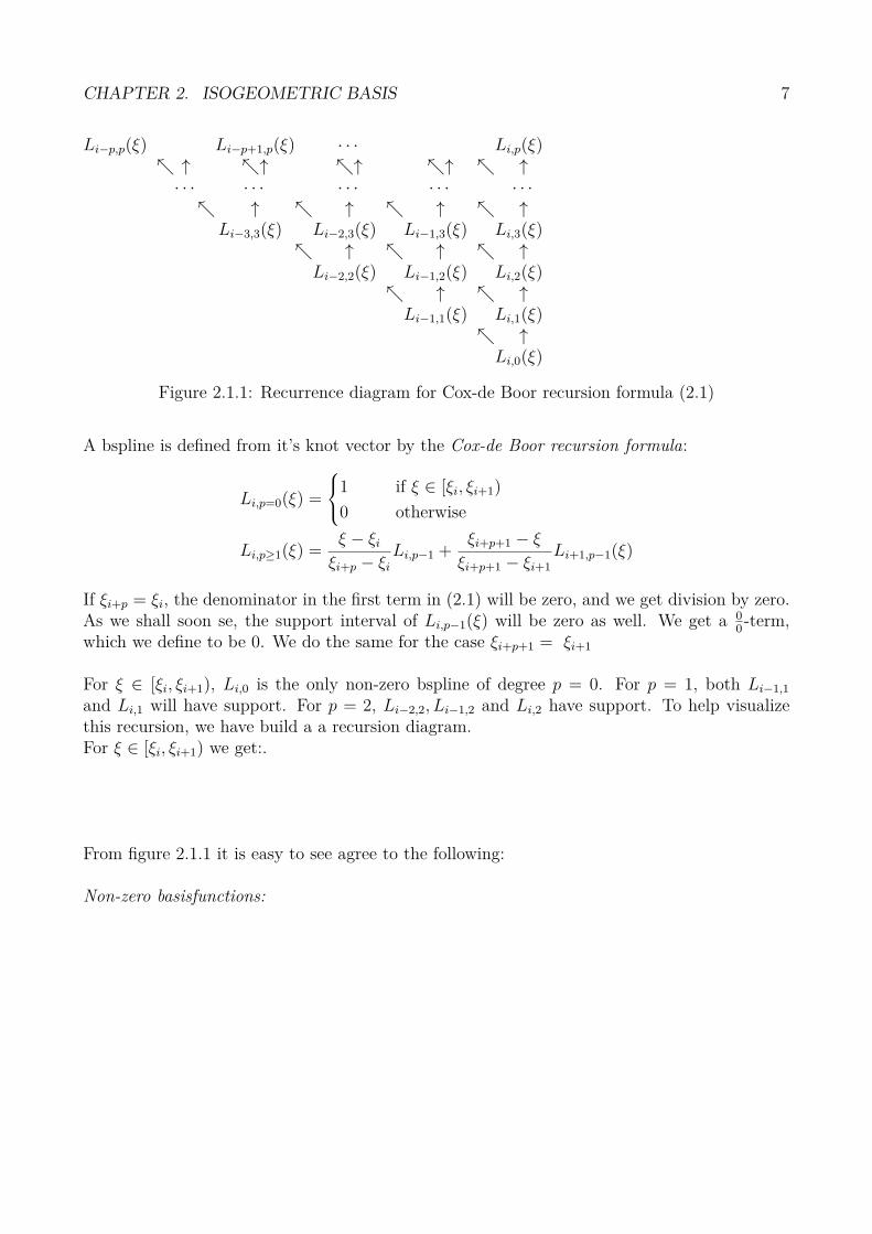
Figure 2.1.1: Recurrence diagram for Cox-de Boor recursion formula (2.1)
A bspline is defined from it’s knot vector by the Cox-de Boor recursion formula:
Li,p=0(ξ) =
1 if ξ ∈ [ξi, ξi+1)
0 otherwise
Li,p≥1(ξ) =ξ − ξi
ξi+p − ξi
Li,p−1 +ξi+p+1 − ξ
ξi+p+1 − ξi+1
Li+1,p−1(ξ)
If ξi+p = ξi, the denominator in the first term in (2.1) will be zero, and we get division by zero.As we shall soon se, the support interval of Li,p−1(ξ) will be zero as well. We get a 0
0-term,
which we define to be 0. We do the same for the case ξi+p+1 = ξi+1
For ξ ∈ [ξi, ξi+1), Li,0 is the only non-zero bspline of degree p = 0. For p = 1, both Li−1,1
and Li,1 will have support. For p = 2, Li−2,2, Li−1,2 and Li,2 have support. To help visualizethis recursion, we have build a a recursion diagram.For ξ ∈ [ξi, ξi+1) we get:.
From figure 2.1.1 it is easy to see agree to the following:
Non-zero basisfunctions:
CHAPTER 2. ISOGEOMETRIC BASIS 8
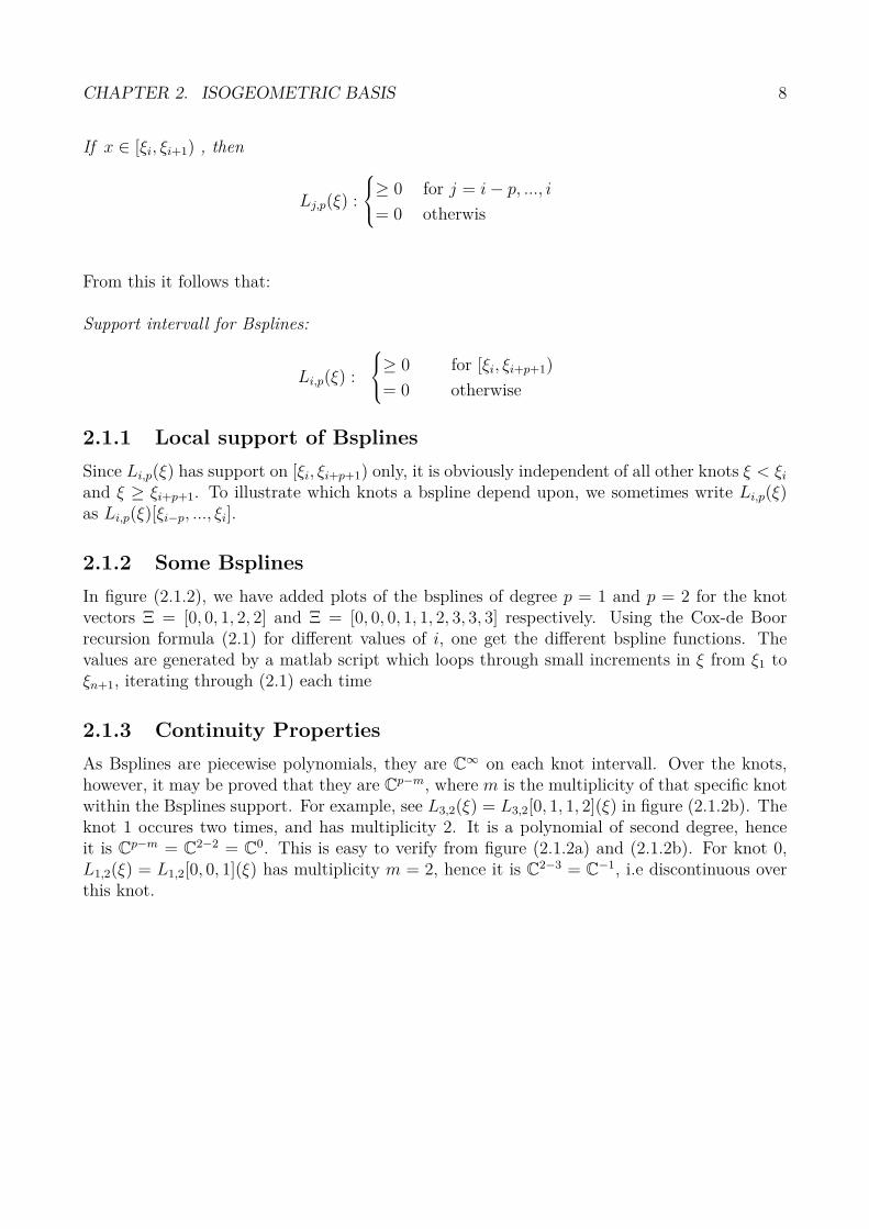
If x ∈ [ξi, ξi+1) , then
Lj,p(ξ) :
≥ 0 for j = i− p, ..., i
= 0 otherwis
From this it follows that:
Support intervall for Bsplines:
Li,p(ξ) :
≥ 0 for [ξi, ξi+p+1)
= 0 otherwise
2.1.1 Local support of Bsplines
Since Li,p(ξ) has support on [ξi, ξi+p+1) only, it is obviously independent of all other knots ξ < ξi
and ξ ≥ ξi+p+1. To illustrate which knots a bspline depend upon, we sometimes write Li,p(ξ)as Li,p(ξ)[ξi−p, ..., ξi].
2.1.2 Some Bsplines
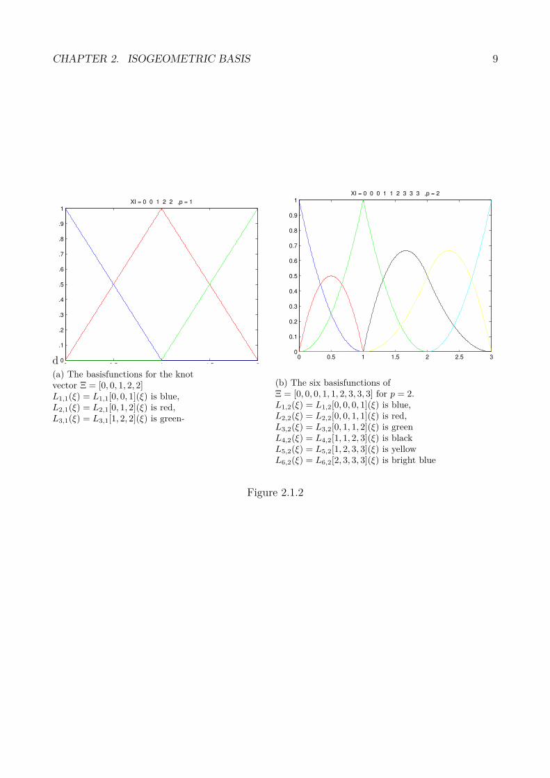
In figure (2.1.2), we have added plots of the bsplines of degree p = 1 and p = 2 for the knotvectors Ξ = [0, 0, 1, 2, 2] and Ξ = [0, 0, 0, 1, 1, 2, 3, 3, 3] respectively. Using the Cox-de Boorrecursion formula (2.1) for different values of i, one get the different bspline functions. Thevalues are generated by a matlab script which loops through small increments in ξ from ξ1 toξn+1, iterating through (2.1) each time
2.1.3 Continuity Properties
As Bsplines are piecewise polynomials, they are C∞ on each knot intervall. Over the knots,
however, it may be proved that they are Cp−m, where m is the multiplicity of that specific knot
within the Bsplines support. For example, see L3,2(ξ) = L3,2[0, 1, 1, 2](ξ) in figure (2.1.2b). Theknot 1 occures two times, and has multiplicity 2. It is a polynomial of second degree, henceit is C
p−m = C2−2 = C
0. This is easy to verify from figure (2.1.2a) and (2.1.2b). For knot 0,L1,2(ξ) = L1,2[0, 0, 1](ξ) has multiplicity m = 2, hence it is C
2−3 = C−1, i.e discontinuous over
this knot.
CHAPTER 2. ISOGEOMETRIC BASIS 9
d0 0.5 1 1.5 2
0
0.1
0.2
0.3
0.4
0.5
0.6
0.7
0.8
0.9
1XI = 0 0 1 2 2 ,p = 1
(a) The basisfunctions for the knotvector Ξ = [0, 0, 1, 2, 2]L1,1(ξ) = L1,1[0, 0, 1](ξ) is blue,L2,1(ξ) = L2,1[0, 1, 2](ξ) is red,L3,1(ξ) = L3,1[1, 2, 2](ξ) is green-
0 0.5 1 1.5 2 2.5 30
0.1
0.2
0.3
0.4
0.5
0.6
0.7
0.8
0.9
1XI = 0 0 0 1 1 2 3 3 3 ,p = 2
(b) The six basisfunctions ofΞ = [0, 0, 0, 1, 1, 2, 3, 3, 3] for p = 2.L1,2(ξ) = L1,2[0, 0, 0, 1](ξ) is blue,L2,2(ξ) = L2,2[0, 0, 1, 1](ξ) is red,L3,2(ξ) = L3,2[0, 1, 1, 2](ξ) is greenL4,2(ξ) = L4,2[1, 1, 2, 3](ξ) is blackL5,2(ξ) = L5,2[1, 2, 3, 3](ξ) is yellowL6,2(ξ) = L6,2[2, 3, 3, 3](ξ) is bright blue
Figure 2.1.2
CHAPTER 2. ISOGEOMETRIC BASIS 10
2.1.4 Partition of unity
The Bsplines Li,p(ξ), i = 1, ..., n defined from the knot vector Ξ = (ξi)l+p+1i=1 form a partition of
unity,i.e
l∑
i=1
Li,p(ξ) = 1
for all ξ ∈ [ξ1, ξn+p+1)
2.1.5 Derivatives of Bsplines
The derivative of a Bspline may easily be found by applying the formula below:
dLi,p
dξ=
p
ξi+p − ξi
Li,p−1(ξ)−p
ξi+p+1 − ξi+1
Li+1,p−1(ξ)
2.1.6 Linear Independence of Bsplines
Bsplines generated from an open knot vectors are linearly independent. From the indexing ofthe nonzero basisfunctions (2.1), we saw that on each intervall [ξi, ξi+1], the p+1 basisfunctionsLi−p,p(ξ), ..., Li,p(ξ) have support. In other words, on each interval there are p + 1 linearlyindependent polynomials of degree p. This means we can span Pp on each subintervall. Hencewe can represent any polynomial of degree p on the intervall [ξ1, ξn+p+1] as a linar combinationof Bsplines
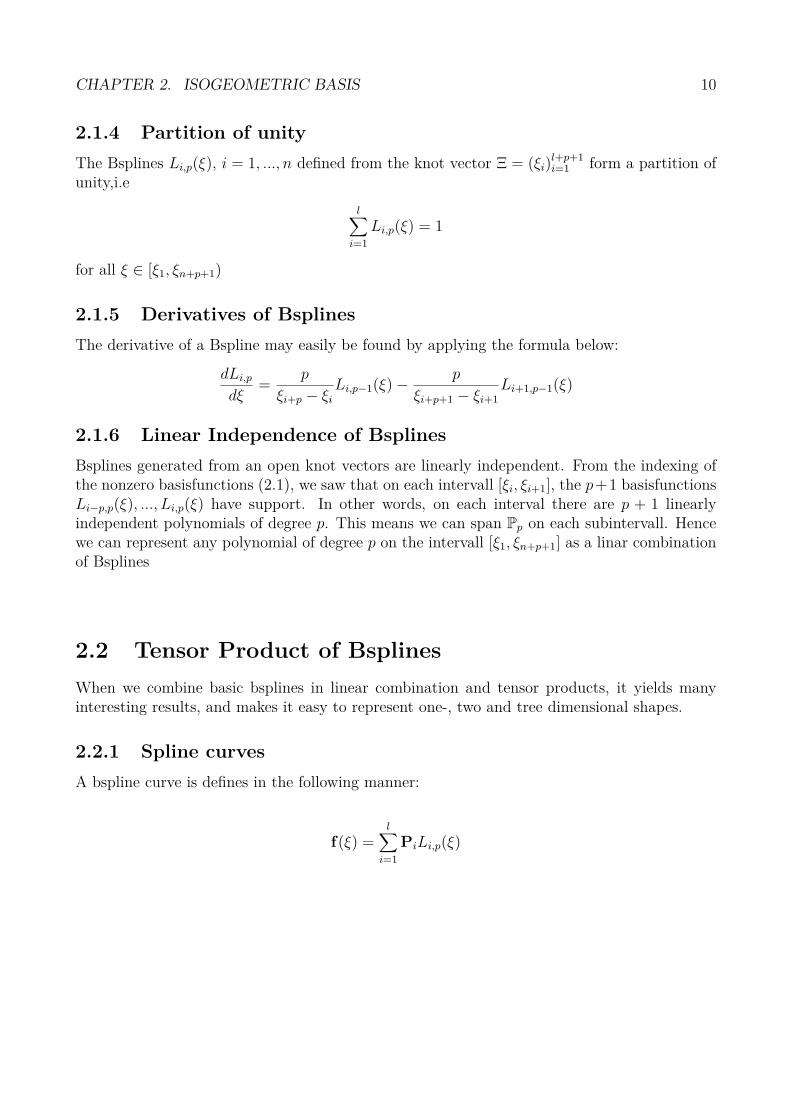
2.2 Tensor Product of Bsplines
When we combine basic bsplines in linear combination and tensor products, it yields manyinteresting results, and makes it easy to represent one-, two and tree dimensional shapes.
2.2.1 Spline curves
A bspline curve is defines in the following manner:
f(ξ) =l∑
i=1
PiLi,p(ξ)

CHAPTER 2. ISOGEOMETRIC BASIS 11
where ci ∈ Rd, d = 1, 2, 3. If d = 1, we get a one dimensional curve. If d = 2 we get a curve in
the plane, and if d = 3 we get a volume curve in space.In two- and three dimensions, Pi are called control points. As
∑li Li,p(ξ) = 1, f(ξ) may be
thought of as a weighted mean of the these control points. Figure 3.1.1 shows an example ofa 2D spline curve. The space of spline curves generated from the knot vector Ξ of degree p isdenoted as
SsΞ,p =
l∑
i=1
PiLi,p(ξ) | Pj ∈ Rs ∀i
−2 −1.5 −1 −0.5 0 0.5 1 1.5 2 2.5 30
0.5
1
1.5
2
2.5
3
3.5
4
Figure 2.2.1: A 2D spline curve from the knot vector [0, 0, 0, 0.25, 0.5, 0.75, 1, 1, 1] The controlpolygon is plotted in red, with the red dots as its control points.

CHAPTER 2. ISOGEOMETRIC BASIS 12
2.2.2 Spline surface
If we let Pi in (2.2.1) be a spline itself, we are left with a spline surface. We insert Pi =∑m
j=1 Pi,jMj,q(η), Pi,j ∈ Rd into equation (2.2.1):
f(ξ, η) =l∑
i=1
m∑
j=1
Pi,jMj,q(η)
Li,p(ξ)
=l∑
i=1
m∑
j=1
Li,p(ξ)Mj,q(η) Pi,j
=l∑
i=1
m∑
j=1
M i,j,p,q(ξ, η) Pi,j
where P ∈ Rs. Hence f : R
2 → Rs. If s = 3 for instance, f is a parametrized surface,
f : (ξ, η)→ (x, y, z)
2.2.3 Spline volumes
A similar argument as for spline surfaces gives us a spline volume.
f(ξ, η, ζ) =l∑
i=1
m∑
j=1
o∑
k=1
Li,p(ξ)Mj,q(η)Ok,r(ζ), Pi,j,k Pi,j,k ∈ Rs
This is a mapping f : R3 → iRs. For s = 3, f is a parametrized volume. This is in fact how wewill represent our configuration Ω over where we wish to solve the elasticity equation.
2.2.4 Control polygon
We have mentioned that the P’s are called control points. The control points form what is calledthe control polygon or the control net. The control polygon can be thought of as a scaffold,or a rough sketch for how the final surface/volume will look like. A 2D control polygon isillustraded in figure 2.2.2
2.2.5 Mapping in FEA
As mentioned in (2.2.3), we will represent our domain is as:
x(ξ, η, ζ) =l∑
i=1
m∑
j=1
o∑
k=1
Li,p(ξ)Mj,q(η)Ok,r(ζ), Pi,j,k Pi,j,k ∈ R3

CHAPTER 2. ISOGEOMETRIC BASIS 13
Figure 2.2.2: A 2D spline area. The red dots are the control points, and are marked with itsassosiated number. They form the control polygon. The blue area is the domain Ω.
CHAPTER 2. ISOGEOMETRIC BASIS 14
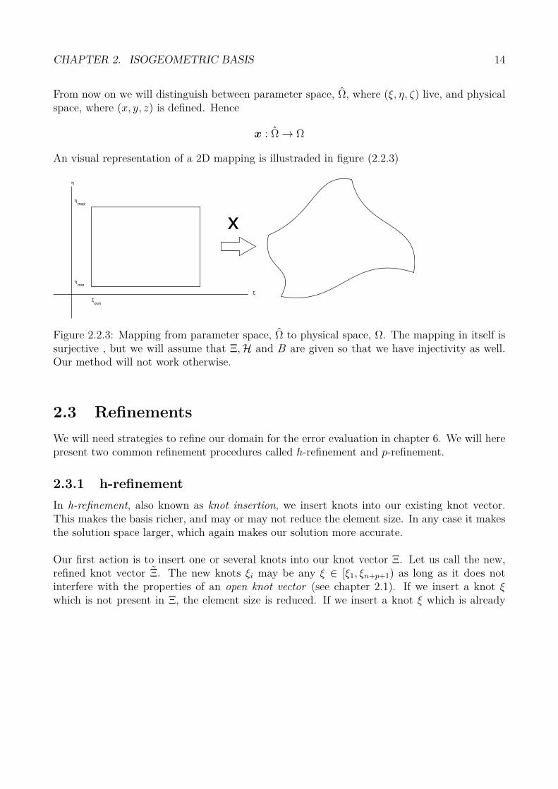
From now on we will distinguish between parameter space, Ω, where (ξ, η, ζ) live, and physicalspace, where (x, y, z) is defined. Hence
x : Ω→ Ω
An visual representation of a 2D mapping is illustraded in figure (2.2.3)
η
ηmax
ηmin
ξmin
ξ
x
Figure 2.2.3: Mapping from parameter space, Ω to physical space, Ω. The mapping in itself issurjective , but we will assume that Ξ,H and B are given so that we have injectivity as well.Our method will not work otherwise.
2.3 Refinements
We will need strategies to refine our domain for the error evaluation in chapter 6. We will herepresent two common refinement procedures called h-refinement and p-refinement.
2.3.1 h-refinement
In h-refinement, also known as knot insertion, we insert knots into our existing knot vector.This makes the basis richer, and may or may not reduce the element size. In any case it makesthe solution space larger, which again makes our solution more accurate.
Our first action is to insert one or several knots into our knot vector Ξ. Let us call the new,refined knot vector Ξ. The new knots ξi may be any ξ ∈ [ξ1, ξn+p+1) as long as it does notinterfere with the properties of an open knot vector (see chapter 2.1). If we insert a knot ξwhich is not present in Ξ, the element size is reduced. If we insert a knot ξ which is already

CHAPTER 2. ISOGEOMETRIC BASIS 15
present, i.e we increase the multiplicity of that knot, we reduce the continuity of the basis.However, the way we choose our new control points will prevent any change to the spline itself.
Assume we are given a spline S ∈ Sp,Ξ. Sp,Ξ ⊆ Sp,Ξ [10], hence any spline S ∈ Sp,Ξ may also berepresented by the basis in Sp,Ξ.
S =l∑
i=1
Li(ξ)ci
=l∑
i=1
M i(ξ)di
where M i, i = 1, ..., l is the basis of Sp,Ξ. In fact, any basisfunctions Li(ξ) ∈ S ∈ Sp,Ξ may berepresented by the basis in S ∈ Sp,Ξ,
Lj(ξ) =l∑
i=1
M iai,j (2.3.1)
We define the vector L =[
L1(ξ), L2(ξ), . . . , Ln(ξ)]
and M =[
M1(ξ), M2(ξ), . . . , M l(ξ)]
This
allows us to write (2.3.1) in vector form:
L = LA
By definning cT = (ci)li=1 and dT = (di)
li=1 we may also write: S = Lc and S = Md Hence
Md = Lc = Ac
which yields d = Ac Matrix A is called the knot insertion matrix of degree p from Ξ to Ξ.
Generation the knot insertion matrix
We will not dig deeper into the theory behind the knot insertion matrix, but simply present analgorithm for how to generating it. The algorithm is build upon theorem 4.6 in [10]. Note thatΞ = (ξi), while Ξ = (ξi).
For i = 1...l......Find µ : ξµ ≤ ξi < ξµ+1
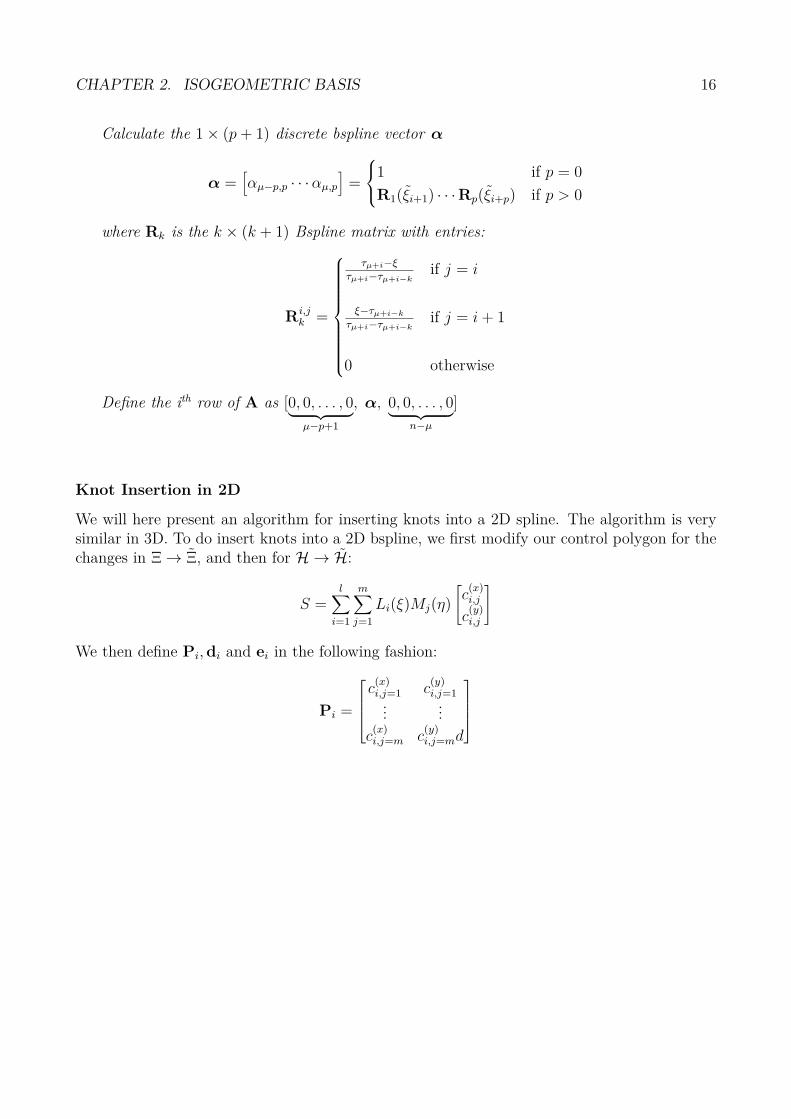
CHAPTER 2. ISOGEOMETRIC BASIS 16
......Calculate the 1× (p + 1) discrete bspline vector α
α =[
αµ−p,p · · ·αµ,p
]
=
1 if p = 0
R1(ξi+1) · · ·Rp(ξi+p) if p > 0
......where Rk is the k × (k + 1) Bspline matrix with entries:
Ri,jk =
τµ+i−ξ
τµ+i−τµ+i−kif j = i
......ξ−τµ+i−k
τµ+i−τµ+i−kif j = i + 1
......
0 otherwise
......Define the ith row of A as [0, 0, . . . , 0︸ ︷︷ ︸
µ−p+1
, α, 0, 0, . . . , 0︸ ︷︷ ︸
n−µ
]
Knot Insertion in 2D
We will here present an algorithm for inserting knots into a 2D spline. The algorithm is verysimilar in 3D. To do insert knots into a 2D bspline, we first modify our control polygon for thechanges in Ξ→ Ξ, and then for H → H:
S =l∑
i=1
m∑
j=1
Li(ξ)Mj(η)
[
c(x)i,j
c(y)i,j
]
We then define Pi, di and ei in the following fashion:
Pi =
c(x)i,j=1 c
(y)i,j=1
......
c(x)i,j=m c
(y)i,j=md

CHAPTER 2. ISOGEOMETRIC BASIS 17
Now, we modify the control points for refinment in η-direction :
S =l∑
i=1
Li(ξ)(
Mci
)T
=l∑
i=1
Li(ξ)(
M(A1ci))T
=l∑
i=1
Li(ξ)(
Mdi
)T
=m∑
j=1
Mj(η)l∑
i=1
Li(ξ)
[
d(x)i,j
d(y)i,j
]
We define dj =
c(x)i=1,j c
(y)i=1,j
......
c(x)i=n,j c
(y)i=n,j
and modify
[
d(x)i,j
d(y)i,j
]
for change in ξ-direction:
S =m∑
j=1
Mj(η)(
Ldj
)T
=m∑
j=1
Mj(η)(
LA2dj
)T
=m∑
j=1
Mj(η)(
Lej
)T
=l∑
i=1
m∑
j=1
Li(ξ)Mj(η)
[
e(x)i,j
e(y)i,j
]
which yields the new lm controlpoints
[
e(x)i,j
e(y)i,j
]
2.3.2 p-refinement
As for h-refinement, a p-refinement of a spline SΞ,H,Z,p,q,r → SΞ,H,Z,p+1,q+1,r+1
must not change
the image of the spline, i.e:
S(ξ, η, ζ) = S(ξ, η, ζ) ∀(ξ, η, ζ) ∈ Ω
To keep the continuity properties of the new splien S, we create the new knot vector Ξ, Hand Z by increasing the multiplicity of each knot in Ξ,H and Z by one. This does not change

CHAPTER 2. ISOGEOMETRIC BASIS 18
the elements in parameter space. From section 2.1.6 we know that on each intervall we canspan any polynomials of order ≤ p. The elements are the same, hence Sp,q,r ⊂ Sp+1,q+1,r+1.The question of creating S is really just a question of choosing the right combination of thebasisfunctions Li(ξ)Mj(η)Ok(ζ) spanning S.
S is a lmo dimensional space, where l, m and o are the number of basisfunctions from theknot vectors Ξ,H and Z respectively. To find the lmo control points needed, we simply do ageneral spline interpolation. We create a system MP = S, where M is a lmo× lmo matrix de-fined as below (2.3.2), P is our matrix of new control points and S the old spline S evaluated inthe interpolation points. To ensure that the system has a unique solution,i.e M is nonsingular,we choose the interpolation points to be
(ξ∗i , η∗
j , ζ∗k) : ξ∗
i =ξi+1 + . . . ξi+(p+1)
(p + 1), η∗
j =ηj+1 + . . . ηj+(q+1)
(q + 1)and ζ∗
j =ζk+1 + . . . ζk+(r+1)
(r + 1)[10]
Here ξi ∈ Ξ, ηj ∈ H and ζk ∈ Z. The system becomes (slett denne setningen: Itilde =(i-1)*(m*o) + (j-1)*o + k;)
L1(ξ∗1)M1(η
∗1)O1(ζ
∗1 ) L1(ξ
∗1)M1(η
∗1)O2(ζ
∗1 ) · · · Ln(ξ∗
1)Mm(η∗1)Or(ζ
∗1 )
L1(ξ∗1)M1(η
∗1)O1(ζ
∗2 ) L1(ξ
∗1)M1(η
∗1)O2(ζ
∗2 ) · · · Ln(ξ∗
1)Mm(η∗1)Or(ζ
∗2 )
L1(ξ∗1)M1(η
∗1)O1(ζ
∗3 ) L1(ξ
∗1)M1(η
∗1)O2(ζ
∗3 ) · · · Ln(ξ∗
1)Mm(η∗1)Or(ζ
∗3 )
......
...L1(ξ
∗n)M1(η
∗m)O1(ζ
∗r ) L1(ξ
∗n)M1(η
∗m)O2(ζ
∗r ) · · · Ln(ξ∗
n)Mm(η∗m)Or(ζ
∗r )
P111...
Plmo
=
S(ξ∗1 , η∗
1, ζ∗1 )
S(ξ∗1 , η∗
1, ζ∗2 )
...S(ξ∗
n, η∗m, η∗
r)
MP = S
(2.3.2)
Both S and P are 3 × lmo matrice, having the control point’s x-coodrinate in column 1, y-coordinate in column 2 and z-coordinate in column 3. We solve (2.3.2) for P, which togetherwith Ξ,H,Z defines our new p-refined spline S.

CHAPTER 2. ISOGEOMETRIC BASIS 19
Figure 2.4.1: The 2D basisfunction N1,2,3,3 and N2,2,3,3 from the knot vectors Ξ = H =[0, 0, 0, 0, 0.5, 1, 1, 1, 1]
2.4 Bsplines as basisfunctiosn in FEA
We will use Bsplines as basisfunctions in our Finite Element Analysis. We defined the scalarbasis function NI as
NI : Ω→ R
NI(ξ, η, ζ) = Li(ξ)Mj(η)Ok(ζ)
The relatoin I (i, j, k) is:
I = (i− 1)mo + (j − 1)o + k
We define the vector basis function, NI , the following way:
NI =
NI
[
1 0 0]T
if I = 1, 4, 7, . . .
NI
[
0 1 0]T
if I = 2, 5, 8, . . .
NI
[
0 0 1]T
if I = 3, 6, 9, . . .
Figure(2.4.1) it is shows a ploit of two 2D scalar basisfunctions.

Chapter 3
Continuum Mechanics
We have assumed an isotrophic and homogenic material.
3.1 Important Definitions
3.1.1 Displacement
The displacement u = u( 0x), is the quantity we directly solve fore in our Isogeometical analysis.
u( 0x) =
u1
u2
u3
is a vector function for how much a particle with positoin 0x before the load
was added will move.
3.1.2 Deformation Gradient
Before we can look deeper into the steps in the lagrangian description, we need to define someterms we will soon need. The first we need to define is the deformation gradient F . Simplysaid, the deformation gradient contains information of deformation and rotation on infinitesimallevel. F is defined in the following manner:
t0F =
∂ tx1
∂ 0x1
∂ tx1
∂ 0x2
∂ tx1
∂ 0x3∂ tx2
∂ 0x1
∂ tx2
∂ 0x2
∂ tx2
∂ 0x3∂ tx3
∂ 0x1
∂ tx3
∂ 0x2
∂ tx3
∂ 0x3
=
∂x∂X
∂x∂Y
∂x∂Z
∂y∂X
∂y∂Y
∂y∂Z
∂z∂X
∂z∂Y
∂z∂Z
t0F iI is the element in row i and column I of F . Note the identity in notation between0x1 = X, 0x2 = Y and 0x3 = Z.
20

CHAPTER 3. CONTINUUM MECHANICS 21
For an infinitesimal vector, d tx = [dx, dy, dz]T it follows from the chain rule that d tx = t0F
0x.
x2
x3
d0x
dtx
x1
Figure 3.1.1: Two infinitesimal arrows, d 0x and d tx. They are related via the linear transfor-mation d tx = t
0Fd tx
Volume
Let us look at an infinitessimally small volume in the original configuration 0Ω, d 0Ω spanned
by the three vectors orthogonal vectors dx1 =
ds100
, dx2 =
0ds20
and dx3 =
00
ds3
. Its volume
is dΩ = (dx1× dx2) · dx3 Since the deformation gradient t0F carries information relation d tx
CHAPTER 3. CONTINUUM MECHANICS 22
to d 0x, it comes a now suprise that is also is used to calculate d tΩ from 0Ω.
d tΩ = det( t0F ) 0dΩ
The deformation tensor
The (right) Cauchy-Green deformation tensor is defined as:
t0C = t
0FT t
0F
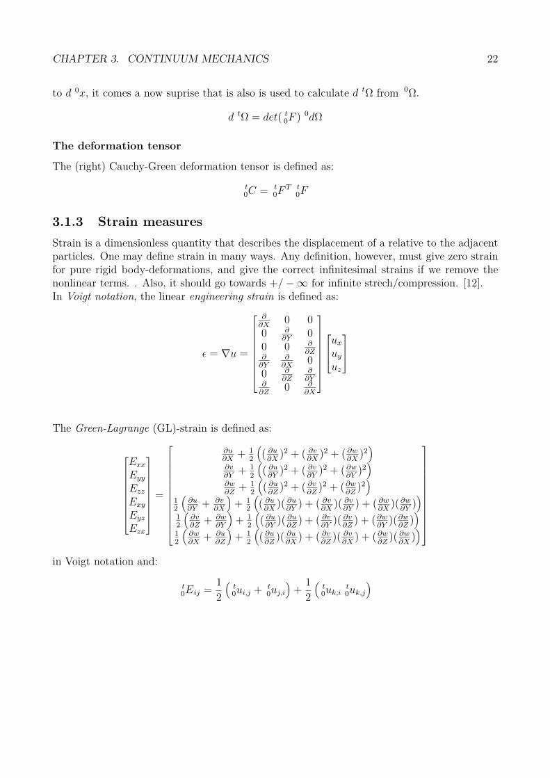
3.1.3 Strain measures
Strain is a dimensionless quantity that describes the displacement of a relative to the adjacentparticles. One may define strain in many ways. Any definition, however, must give zero strainfor pure rigid body-deformations, and give the correct infinitesimal strains if we remove thenonlinear terms. . Also, it should go towards +/−∞ for infinite strech/compression. [12].In Voigt notation, the linear engineering strain is defined as:
ǫ = ∇u =
∂∂X
0 00 ∂
∂Y0
0 0 ∂∂Z
∂∂Y
∂∂X
00 ∂
∂Z∂
∂Y∂
∂Z0 ∂
∂X
ux
uy
uz
The Green-Lagrange (GL)-strain is defined as:
Exx
Eyy
Ezz
Exy
Eyz
Ezx
=
∂u∂X
+ 12
(
( ∂u∂X
)2 + ( ∂v∂X
)2 + ( ∂w∂X
)2)
∂v∂Y
+ 12
(
( ∂u∂Y
)2 + ( ∂v∂Y
)2 + ( ∂w∂Y
)2)
∂w∂Z
+ 12
(
( ∂u∂Z
)2 + ( ∂v∂Z
)2 + (∂w∂Z
)2)
12
(∂u∂Y
+ ∂v∂X
)
+ 12
(
( ∂u∂X
)( ∂u∂Y
) + ( ∂v∂X
)( ∂v∂Y
) + ( ∂w∂X
)( ∂w∂Y
))
12
(∂v∂Z
+ ∂w∂Y
)
+ 12
(
( ∂u∂Y
)( ∂u∂Z
) + ( ∂v∂Y
)( ∂v∂Z
) + ( ∂w∂Y
)(∂w∂Z
))
12
(∂w∂X
+ ∂u∂Z
)
+ 12
(
( ∂u∂Z
)( ∂u∂X
) + ( ∂v∂Z
)( ∂v∂X
) + (∂w∂Z
)( ∂w∂X
))
in Voigt notation and:
t0Eij =
1
2
(t0ui,j + t
0uj,i
)
+1
2
(t0uk,i
t0uk,j
)
CHAPTER 3. CONTINUUM MECHANICS 23
on tensor form. Other, equivalent definitions are:
t0E =
1
2( t
0C − I)
Eij =1
2(F iJF iJ − δIJ)
3.1.4 Stress (measures)
We will use two stress measures in this project, Cauchy stress and second Piola-Kirchhoff stress(PK2).
Cauchy stress, denoted σ, is defined as current force divided by current area. [12]. It isthe true, physical stress that arises in a physical configuration when it is subjected to stress.The PK2-stress is a useful theoretical quantity which is defined as current force mapped intothe reference configuration divided by a reference area. [18]. The relation between Cauchystress and PK2 stress is:
σij =1
JF iIF jJSIJ (3.1.1)
where J = det(F ). [11].
3.1.5 Traction
Traction is cauchy stress that is assosiated with a surface. This surface could be a given surfacewithin the configuration, or the outer surface of the configuration. [4]

Chapter 4
Linear Elasticity
We will start our approach towards nonlinear finite element analysis by looking at the linearfinite element method. The Updated Lagrangian Description we will use later builds upon thismethod. Linear Finite Element analysis leans upon the assumptions of a the linear materiallaw and a liner strain displacement relation. The first assumption requires small strains, whilethe latter requires small displacements.
We will now derive the linear elasticity equation,∇u = −f , as this gives a fundamental under-standing of the physical problem. From the linear elasticity equation we will derive the weakfrom, from wich we will eventually assebmle the linear system.
4.1 Deriving the linear elasticity equation
In our static analysis we will consider two kinds of forces action on our body; body forces andtraction forces. Body forces are forces that acts on the body itself, like magnetic forces, gravi-tation forces or forces arising from thermal expansion. The traction forces act on the boundaryof our body, like weight upon a bridge.
Figure (4.1.1) shows a principal 2D sketch of an infinitesimally small element within a configura-tion (domain), subjected to body forces f and traction forces σ along its borders. For a similar
3D infinitesimal element, we define We define σx =[
σxx σxy σxz
]T, σy =
[
σyx σyy σyz
]T
24

CHAPTER 4. LINEAR ELASTICITY 25
∆y
∆x
-σy(x, y - )
(x,y)
∆y
2
σy(x, y + )∆y
2
-σx(x - , y)∆x
2
σx(x + , y)∆x
2
σyy
σyx
σxy
σxx
Figure 4.1.1: Forces acting on an infinitesimal element. The figure is insipred by figure 9.3 in[4]
and[
σzx σzy σzz
]T. The basic static equalibrium equations yield;
−∆y∆z σx(x−∆x
2, y, z) + ∆y∆z σx(x +
∆x
2, y, z)
−∆x∆z σy(x, y −∆y
2, z) + ∆x∆z σy(x, y +
∆y
2, z)
−∆x∆y σz(x, y, z −∆z
2) + ∆x∆y σz(x, y, z +
∆z
2)
= −f(x, y, z)∆x∆y∆z
where f(x, y, z) is the body force pr. unit area. We divide by ∆x∆y∆z. As ∆x and ∆y go

CHAPTER 4. LINEAR ELASTICITY 26
towards zero, we get:
1
∆x
(
−σx(x−∆x
2, y, z) + σx(x +
∆x
2, y, z)
)
1
∆y
(
−σy(x, y −∆y
2, z) + σy(x, y +
∆y
2, z)
)
1
∆z
(
−σz(x, y, z −∆z
2) + σz(x, y, z +
∆z
2)
)
= −f(x, y, z)
∆x→ 0 , ∆y → 0 and ∆z → 0⇒
∂σx
∂x+
∂σy
∂y+
∂σz
∂z= −f
[∂
∂x∂
∂y∂∂z
]
σx
σy
σz
= −f
[∂
∂x∂
∂y∂
∂x
]
σxx σxy σxz
σyx σyy σyz
σzx σzy σzz
= −
fx
fy
fz
[∂
∂x∂
∂y∂
∂x
]
σxx σyx σzx
σxy σyy σzy
σxz σyz σzz
= −
fx
fy
fz
∇σ = −f
Note that σij is a symmetric stress tensor, i.e σij = σji.We have now arrived with the problem we wish to solve in linear elasticity:
Find u such that:
∇σ(u) = −f (4.1.1)
u = uD on ΓD
σ n = h on ΓN
where σ = Cǫ(u) = C∇uf

CHAPTER 4. LINEAR ELASTICITY 27
4.2 Deriving the weak form
We will now derive its the weak form of problem (4.1.1). The theory in this section is in cor-relation with [4].
We will here utilize the geometrical relationship between ǫ and u, and the physical relationshipbetween σ and u. We search for a u ∈ R
3 such that σ(u) forfills (4.1.1). The derivatives ofu will later be integrated, so we define the solution space to consist of those u where that aresuited for this;
u ∈ U = u|u ∈ H1, u = uD on ΓD
∇σ(u) is a vector, hence (4.1.1) is a system of the three equations:
∂σ11
∂x1
+∂σ21
∂x2
+∂σ31
∂x3
= −f1
∂σ12
∂x1
+∂σ22
∂x2
+∂σ32
∂x3
= −f2
∂σ13
∂x1
+∂σ23
∂x2
+∂σ33
∂x3
= −f3
(slett: (Jacob fish s. 67, s. 224). ) We multiply each of these two equations by a testfunctionvi ∈ V . We define V = Hk(Ω) = f ∈ L2(Ω) : Dαf ∈ L2(Ω)∀α : |α| ≤ k to ensure that allthe integrals that contain vi are well defined.
∂σ11
∂x1
v1 +∂σ21
∂x2
v1 +∂σ31
∂x3
v1 = −f1v3
∂σ12
∂x1
v2 +∂σ22
∂x2
v2 +∂σ32
∂x3
v2 = −f2v3
∂σ13
∂x1
v3 +∂σ23
∂x2
v3 +∂σ33
∂x3
v3 = −f3v3
We integrate over Ω and add the terms together: :
3∑
i=1
3∑
j=1
∫
Ω
∂σij
∂xi
vj dΩ = −3∑
j=1
∫
Ωfjvj dΩ (4.2.1)
The formula for integration by parts for higher dimensions states,∫
Ω
∂σij
∂xi
vj dΩ =∫
Γσijvjni dΓ−
∫
Ωσij
∂vj
∂xi
dΩ

CHAPTER 4. LINEAR ELASTICITY 28
where ni is the i-th component of the outward normal vector n at that point on Γ. We applythis identity into (4.2.1):
3∑
i=1
3∑
j=1
∫
Ω
∂σij
∂xi
vj dΩ = −3∑
j=1
∫
Ωfjvj dΩ
3∑
i=1
3∑
j=1
∫
Γσijvjni dΓ−
3∑
i=1
3∑
j=1
∫
Ωσij
∂vj
∂xi
dΩ = −3∑
j=1
∫
Ωfjvj dΩ
3∑
i=1
3∑
j=1
∫
Ωσij
∂vj
∂xi
dΩ =3∑
j=1
∫
Ωfjvj dΩ +
3∑
i=1
3∑
j=1
∫
Γσijvjni dΓ (4.2.2)
Note that, according to the linear relation between engineering strain ǫij and u,
ǫij(v) =
∂vi
∂xjif i = j
∂vi
∂xj+ ∂vj
∂xiif i 6= j
We apply this relation to equation (4.2.2):
3∑
i=1
3∑
j=1
∫
Ωσij
∂vj
∂xi
dΩ =3∑
j=1
∫
Ωfjvj dΩ +
3∑
i=1
3∑
j=1
∫
Γσijvjni dΓ
3∑
i=1
3∑
j=i
∫
Ωσijǫij dΩ =
3∑
j=1
∫
Ωfjvj dΩ +
3∑
i=1
3∑
j=1
∫
Γσijvjni dΓ
Using Voigt notation,
ǫ =
ǫ11
ǫ22
ǫ33
ǫ12
ǫ23
ǫ31
, σ =
σ11
σ22
σ33
σ12
σ23
σ31
f =
f1
f2
f3
we get:
∫
ΩǫT (v)σ(u) dΩ =
∫
ΩvTf dΩ +
∫
ΓvT σn dΓ
We then insert σ = Cǫ(u)

CHAPTER 4. LINEAR ELASTICITY 29
∫
ΩǫT (v)Cǫ(u) dΩ =
∫
ΩvTf dΩ +
∫
ΓD
vT σn dΓ +∫
ΓN
vT σn dΓ
The weak form becomes:
Weak form:
Find u ∈ V such that
a(u, v) = F (v) ∀v ∈ V (4.2.3)
where
a(u, v) =∫
ΩǫT (v)Cǫ(u) dΩ
F (v) =∫
ΩvTf dΩ +
∫
ΓvT σn dΓ
V = v|v ∈ H1, v = 0 on ΓD
4.2.1 Galerkin method
Lax-Milgram’s lemma states that there exist one unique solution to (4.2.3). However, the spaceV may be infinite dimensional, and the task (4.2.3) of finding a function u that works for allv ∈ V may be far beyond reach. We therefor approximate V to finite dimensional subspace:
V h = vh | vh ∈ H1(Ω), vh|Γ = 0 ⊆ V
Hence, we reformulate equation (4.2.3) to:
Weak form (discrete). Find uh ∈ V h such that
a(uh, vh) = F (vh) ∀vh ∈ V h (4.2.4)

CHAPTER 4. LINEAR ELASTICITY 30
Since we use an approximating to the possibly infite space V , the answer of problem (4.2.4)will in general no longer give us the exact answer. It can however be shown that the solutionof problem (4.2.4) will always be the best possible solution within that space [15]. By bestpossible we mean the solution that minimizes the energy norm ||uexact − uh||a.
4.3 Assembling the linear system
Given (4.2.4), we want to assemble a linear system we can solve using matix manipulation.According to our choise of basisfunctions, we may write the possible displacement fields u as
u = NU = NIUI (4.3.1)
where N = [N1N2, ..., N3lmo] and the repeated index imply summation. Also, we may write thetest function v as
v = NV = NJVJ
since they come from the same function space. U and V are here two coefficient vectors. Weinsert (4.3.1) into (4.2.4):
a(NIUI , v) = F (v) ∀v ∈ V h
a(NI , v)UI = F (v) ∀v ∈ V h
This must hold for all v ∈ V h, which is equivalent of saying that it must hold for all thebasisfunctions spanning V h. Since a and F are bilinear and linear respectivly, and V h =spanN1, N2, ...NNndof
, we get:
a(N1, N1) a(N2, N1) ... a(Nndof , N1)a(N1, N2) a(N2, N2) ... a(Nndof , N2)
. . .a(N1, Nndof ) a(N2, Nndof ) ... a(Nndof , Nndof )
U1
U2...
Undof
=
F (N1)F (N2)
...F (Nndof )
(4.3.2)
Av = F
where A is the stiffness matrix. Implementation detilas for A and F can be found in AppendixC.
4.4 Boundary conditions
In this thesis we have consider homogeneous dirichlet boundary conditions and neumann bound-ary conditions. Homogeneous dirichlet boundary conditions represent areas there the configura-tion is fixed. Neumann boundary condtions represent areas where the configuration is subjected
CHAPTER 4. LINEAR ELASTICITY 31
to pressure.
4.4.1 Dirichlet Boundary Conditions
The solution u(x, y, z) must be zero on the areas where we have homogeneous dirichlet bound-ary conditions. We do this by simply removing those basisfunctions NI which has support overthis area from the linear system (4.3.2). Or more accurately, we never even calculate them,and remove their corresponding rows and columns.
Note that without dirichet boundary conditions, six of the eigenvalues of the stiffness matrixA will be zero (the six degrees of freedom). A will be singular, and we will not get a solution.
4.5 Neumann boundary Conditions
The neumann conditions along the boundary, σ · n = h on ΓN , ends up as a part on the loadvector F via the integral
∫
ΓNNT
J σn dΓ. Evaluation of this integral is described in AppendixC.
Chapter 5
Nonlinear Finite Element Analysis
We will now take the leap to nonlinear finite element analysis. When the deformation of theconfiguration becomes large, the linear strain-displacement relationship we have used so farbecomes inaccurate. Also, changes in volume and shape may be inadmissible to neglect.
In a nonlinear finite element method, the load is typically divided into load increments. Foreach load step we use some form of numerical method to iterate until we get the satisfiedaccuracy. A graphical representation of this technique is shown in figure (5.0.1).
5.0.1 Variational Formulations
There are two common variational descriptions for the nonlinear problem. The first is calledthe total lagrangian (TL) formulation. The total lagrangian formulation uses the original con-figuration as reference configuration, and the energetically conjugate Green-Lagrange strainand the PK2 stress tensor are normally used.
The other formulation is called the Updated Lagrangian (UL) formulation. The UL formulationuses the current configuration as reference configuration. We have programmed a nonlinearisogeometric solver in Matlab using the UL formulation. We will therefore go through themathematical theory behind the UL formulation in some detail. This will eventually result inthe nonlinear algorithm underlying our Matlab code.
5.1 Updated Lagrange
The updated lagrangian description is a variational description where we may use a nonlinearstrain-displacement law and a nonliner stress-strain relation. In this project, we have looked at
32

CHAPTER 5. NONLINEAR FINITE ELEMENT ANALYSIS 33
3F
2F
1F
1U
2U
3U
U
F
Figure 5.0.1: A principle sketch of the load path, were we add the load vector R in increments.This figure is is a modified version of figure (2.5) in [8]

CHAPTER 5. NONLINEAR FINITE ELEMENT ANALYSIS 34
nonlinearity in strain only, and we will use a linear stress-strain law.
The following theory and notation is compiled from [1]. Note that this notation may differ atsome points from more commonly used nomenclature. For a introduction to the notation, seeAppendix A.
5.1.1 Weak form
We will derive the weak for the updated lagrangian description by using the principle of virtualdisplacement. This principle relies on the fact that, for a given perturbation of the configuration,the sum internal work must equal the sum external work.
δWint = δWext
For small perturbation, the work induced by the stress variation has neglectable influence.Hence
∫
t+∆tΩδ t+∆teij
t+∆tσijt+∆tdΩ =
∫
t+∆tΩ(δu)T t+∆tf t+∆tdΩ +
∫
t+∆tΓ(δu)T t+∆th t+∆tdΓ
= t+∆tR (5.1.1)
This left hand side of (5.1.1) is energy conjugate to∫
tΩ δ t+∆ttEij
t+∆ttSij
tdΩ. This yields:∫
tΩδ t+∆t
tEijt+∆t
tSijtdΩ = t+∆tR (5.1.2)
Note the following relations of the PK2 stress and nonlinear strain:
t+∆ttSij = t
tSij + tSij = tσij + tSij (5.1.3)t+∆t
tEij = ttEij + tEij = tEij (5.1.4)
tEij is the strain increment from configuration tΩ to t+∆tΩ. tu is the corresponding incrementin displacement. This gives ut the expression for tEij:
tEij =1
2( tui,j + tuj,i) +
1
2( tuk,i tuk,j) (5.1.5)
Repeated indices imply summation, and tui,j means ∂ui
∂ txj. The first term in (5.1.5) is linear in
ui, while the second term is nonlinear in ui. We now split the strain into two parts, one linearand one nonlinear.
tEij =1
2( tui,j + tuj,i) +
1
2( tuk,i tuk,j)
= tǫij + tβij (5.1.6)
CHAPTER 5. NONLINEAR FINITE ELEMENT ANALYSIS 35
The strain increments induced from a small perturbation δu becomes:
δ tEij = δ tǫij + δ tβij
δ tǫij =1
2(( tu + δ tu)i,j + ( tu + δ tu)j,i)−
1
2( tui,j + tuj,i)
=1
2(δ tui,j + δ tuj,i) (5.1.7)
Note that ǫij is a constant for a given virtual displacement δu. A similar argument reveals thatδ tβij is linear in ui:
δ tβij =1
2(( tu + δ tu)k,i( tu + δ tu)k,j)−
1
2( tuk,i tuk,j)
=1
2( tuk,i tuk,j + tuk,iδ tuk,j + δ tuk,i tuk,j + δ tuk,iδ tuk,j)−
1
2( tuk,i tuk,j)
=1
2( tuk,iδ tuk,j + δ tuk,i tuk,j) (5.1.8)
We then insert expressions from (5.1.3) (5.1.4) and (5.1.6) into (5.1.2):∫
tΩδ t+∆t
tEijt+∆t
tSijtdΩ = t+∆tR
∫
tΩ(δ tǫij + δ tβij)(
tσij + tSij)tdΩ = t+∆tR
∫
tΩδ tǫij
tσij + δ tβijtσij + (δ tǫij + δ tβij) tSij
tdΩ = t+∆tR∫
tΩδ tǫij
tσijtdΩ +
∫
tΩδ tβij
tσijtdΩ +
∫
tΩδ tEij tSij
tdΩ = t+∆tR
Until now, all we have done is continuum mechanics. As we mentioned in the beginning of thischapter, we will add the external loads incrementally. The load vector R is a function of time.We first solve the load vector t1R, then add the load increment ∆R = t2R− t1R and solve thesystem again. Figure (5.0.1) illustrates the procedure. This means that for a given time t, tU ,tΩ and tσ are all known. We move the known quantities to the right hands side and keep theunknown integrals on the left hand side:
∫
tΩδ tβij︸ ︷︷ ︸
unknown
tσijtdΩ
︸ ︷︷ ︸
known
+∫
tΩδ tEij︸ ︷︷ ︸
unknown
tSijtdΩ
︸ ︷︷ ︸
unknown
= t+∆tR︸ ︷︷ ︸
known
−∫
tΩδ tǫij︸ ︷︷ ︸
known
tσij︸︷︷︸
known
tdΩ
This is actually our weak formulation:
CHAPTER 5. NONLINEAR FINITE ELEMENT ANALYSIS 36
Weak form:
Find tu such that
∫
tΩδ tEij tSij
tdΩ +∫
tΩδ tβij
tσijtdΩ = t+∆tR−
∫
tΩδ tǫij
tσijtdΩ
(5.1.9)
for any small virtual displacement δu.
5.2 Linearisation and discretisation
Since we will do this with the finite element method, we somehow need to transform (5.1.9)into a linear system. The weak form (5.1.9) contains nonlinear terms. We will now show welinearise them and obtain a system on the form
ttK∆U = t+∆t
t+∆tR−ttF
where ttK is the tangent stiffness matrix, t+∆t
t+∆tR is the external force vector at time t + ∆t, andttF is the internal force vector at time t.
5.2.1 The integral∫
tΩ δ tEij tSijtdΩ
In this thesis, we use a linear stress-strain relation. The stress increment is tSij = tCijrs tErs,where tCijkl is the material moduli in the current configuration. We linearise the integral inthe following manner:
∫
tΩδ tEij tSij
tdΩ =∫
tΩδ tEij tCijrs tErs
tdΩ
=∫
tΩ(δ tǫij + δ tβij) tCijrs( tǫrs + tβrs)
tdΩ
≈∫
tΩδ tǫij tCijrs tǫrs
tdΩ (5.2.1)
Here we approximated tEij ≈ tǫij and δ tEij ≈ δ tǫij. This approximation holds whenever thetime between two load increments small, i.e whenever ∆t is small.

CHAPTER 5. NONLINEAR FINITE ELEMENT ANALYSIS 37
Assembly of∫
tΩ δ tǫijCijrs tǫrstdΩ
The vectors tu, tǫ and there virtual pairs are defined as follows:
tu = tN∆U
δ tu = tNδU
tǫ = ∇ tu = ∇ tN∆U = B∆U
δ tǫ = BδU
We arrange the tensor tCijrs into matrix form in the following manner.
tC =
tC1111 tC1122 tC1133 0 0 0
tC2211 tC2222 tC2233 0 0 0
tC3311 tC3322 tC3333 0 0 00 0 0 tC1212 0 0 00 0 0 0 tC2323 0 00 0 0 0 0 tC3131
The integral under consideration (5.2.1) becomes:∫
tΩδ tǫij tC tǫrs
tΩ =∫
tΩ(δ tǫ
T ) tC( tǫ)tdΩ
=∫
tΩδUT BT
tCB∆U tdΩ
= δUT
(∫
tΩBT
tCijrsBtdΩ
)
∆U
= δUTtKM∆U
where the material stiffness matrix KM is defined as tKM =∫
tΩ BTtCijrsB
tdΩ
5.2.2 The integral∫
tΩ δ tβijtσij
tdΩ
As we saw in (5.1.8), δ tβij is a linear term. Since tσij is known, this integral is linear withrespect to ui.
Assembly
We want to discretise this integral into a linear system. tβ, the nonlinear part of the strainincrement we defined in (5.1.6):
tβ =1
2( tuk,i tuk,j)

CHAPTER 5. NONLINEAR FINITE ELEMENT ANALYSIS 38
In voight notation, when it is discretized, we write:
∂ tu
∂ txi
= tu.,i =
∂ tu1
∂ txi∂ tu2
∂ txi∂ tu3
∂ txi
=∂ tN∆U
∂ txi
=∂ tN
∂ txi
∆U
=
∂N1
∂ txi0 0 ∂N2
∂ txi0 0 ...
0 ∂N1
∂ txi0 0 ∂N2
∂ txi0 ...
0 0 ∂N1
∂ txi0 0 ∂N2
∂ txi...
∆U1
∆U2
...
∆UNbf
Note that I refer to a scalar basis function NI(x, y, z) ∈ R, while I refer to the vector basisfunction NI(x, y, z) ∈ R
3. I = 1, ..., lmo, while I = 1, ..., 3lmo. See Appendix A for the relationI ∼ I.
tuk,i =∂NI
∂ txi
∆UI(I) (sum over I) (5.2.2)
δ tuk,i =∂NI
∂ txi
δUI(I) (sum over I) (5.2.3)
The definition of δβ is from (5.1.8)
δ tβij =1
2(δ tuk,i tuk,j) +
1
2( tuk,iδ tuk,j) (5.2.4)
We insert expression (5.2.2) and (5.2.3) to (5.2.4)
δ tβijtσij =
1
2(δ tuk,i tuk,j + tuk,iδ tuk,j)
tσij
=1
2
(
tN I,iδUI(I) tN J ,j∆UJ(J) + tN I,i∆UI(I) tN J ,jδUJ(J)
)tσij
= tN I,iδUI(I) tN J ,j∆UJ(J)tσij
= δUI(I)
(
tN I,itσij tN J ,j
)
∆UJ(J)

CHAPTER 5. NONLINEAR FINITE ELEMENT ANALYSIS 39
Hence:∫
tΩ
tσijδ tβijtdΩ =
∫
tΩδUI(I)
(
tN I,itσij tN J ,j
)
∆UJ(J)tdΩ
= (δU)T
ttG11
ttG12
ttG13 ... t
tG1NbfttG21
ttG22
ttG23 ... t
tG2Nbf
...ttGNbf 1
ttGNbf 2
ttGNbf 3 ... t
tGNbf Nbf
∆U
(5.2.5)
where ttGIJ is a 3× 3 block matrix:
ttGIJ = I(3×3)
∫
tΩtN I,i
tσij tN J ,jtdΩ
We define
ttKG =
ttG11
ttG12
ttG13 ... t
tG1NbfttG21
ttG22
ttG23 ... t
tG2Nbf
...ttGNbf 1
ttGNbf 2
ttGNbf 3 ... t
tGNbf Nbf
(5.2.6)
Hence equation (5.2.5) becomes
∫
tΩ
tσijδ tβijtdΩ = δUT t
tKG∆U
Details for how to calculate KG may be found in Appendix D).
5.2.3 Assembly of∫
tΩ δ tǫijtσij
tdΩ
For a given δu, all the therm in the integral∫
tΩ δ tǫijtσij
tdΩ are known. δ tǫij is given byequation (5.1.7). We discretize it the following way:
δ tǫ = ∇( tu + δ tu)−∇ tu = ∇δ tu = ∇ tNδ tU = Bδ tU
∫
tΩδ tǫij
tσijtdΩ =
∫
tΩδ tǫ
T tσ tdΩ
= δ tUT∫
tΩBT tσ tdΩ
= δ tUT t
tF

CHAPTER 5. NONLINEAR FINITE ELEMENT ANALYSIS 40
5.2.4 The external virtual work
t+∆ttR =
∫
tΩδui
t+∆tf itdΩ +
∫
tΩδui
t+∆th tdΩ
=∫
tΩδuT t+∆tf tdΩ +
∫
tΩδuT t+∆th tdΩ
=∫
tΩδUT
tNT t+∆tf tdΩ +
∫
tΩδUT
tNT t+∆th tdΩ
= δUT
(∫
tΩtN
T t+∆tf tdΩ +∫
tΩtN
T t+∆th tdΩ
)
= δUT t+∆ttR
where f is the body force, and h is the traction force.We will now summarize what we have done on the previous pages to form the linear systemttKT ∆U = R− F .
5.3 Assembling the linear system
From equation (5.1.9) we had the following equation:
Find tu such that
∫
tΩδ tβij
tσijtdΩ +
∫
tΩδ tǫij tSij
tdΩ = t+∆tR−∫
tΩδ tǫij
tσijtdΩ
for any small virtual displacement δu.
We now insert the discretized versions of each on the integrals in (5.3). This gives us:
∫
tΩδ tβij
tσijtdΩ +
∫
tΩδ tǫij tSij
tdΩ = t+∆tR−∫
tΩδ teij
tσijtdΩ
δUT ttKG∆U + δUT
tKM∆U = δUT t+∆ttR− δ tUT t
tF
δUT(
ttKG + tKM
)
∆U = δUT(
t+∆ttR−
ttF)
This must hold for any virtual displacement δu = tNδU , hence it must hold for any δU . Thisis equivalent to say that the following equality must hold:

CHAPTER 5. NONLINEAR FINITE ELEMENT ANALYSIS 41
ttKT ∆U = t+∆t
tR−ttF (5.3.1)
where
t+∆ttR =
∫
tΩtN
T t+∆tf tdΩ +∫
tΩtN
T t+∆th tdΩ
ttF =
∫
tΩBT C t
0ǫtdΩ
ttKT = tKM + t
tKG,
tKM =∫
tΩBT CijrsB
tdΩ
and ttKG is defined as in (5.2.6). Impementation details for F and
5.4 Comments to the linear system
The linear system (5.3.1) does not represent (5.1.9) perfectly, in that the second intergral in(5.1.9),
∫
tΩ δ tǫij tSijtdΩ, has been linearized. As mentioned in (5.2.1), this approximation is
good when tu is small. To assure this, we will divide the external load, the body force f andthe traction force h into many load steps
5.5 The Nonlinear Algorithm
The algorithm we present here is the core of our matlab code. For each load case, the algorithmcalculates the terms in (5.3.1), solve for ∆U , and update the configuration. It iterates untilequalibrium, and start over again on the next load increment.Start with configuration t0Ω.
for time t = t1, t2, ..., tn.......(We have tU, tΩ)......(We wish to find t+∆tU : t+∆tF ( t+∆tU) = t+∆t
t+∆tF = t+∆tt+∆tR.)
......(We know (from last time step) that ttF = t
tR)
......Update the external forece vector according to the new load;
............ t+∆ttR =
∫
tΩ tNT t+∆tf i
tdV +∫
tΓ tNT t+∆thi
tdΓ

CHAPTER 5. NONLINEAR FINITE ELEMENT ANALYSIS 42
......Calculate ttKT = tKM + t
tKG,............ tKM =
∫
tΩ BT CB tdV .
............ ttK
abG = I3×3
∫
tΩ tNa,itσij tN b,j
tdV
......Set t+∆tt+∆tF
(0) = ttF , t+∆t
t+∆tR(0) = t+∆t
tR, t+∆tU (0) = tU and k = 1.
...... t+∆tt+∆tK
(0)T = t
tK.
......r(0) = t+∆tt+∆tR
(0) − t+∆tt+∆tF
(0) (out of balance term)......While ||r(k−1)|| > tol
............Find ∆U (k) : t+∆tt+∆tK
(k−1)T ∆U (k) = r(k−1)
............ t+∆tU (k) = t+∆tU (k−1) + ∆U (k)
............Update t+∆tΩ
............Calcualte t+∆tt+∆tK
(k)T
............Calculate t+∆tt+∆tR
(k)
............Calculate t+∆tt+∆tF
(k) (see D.2).
............r(k) = t+∆tt+∆tR
(k) − t+∆tt+∆tF
(k)
............k = k + 1
......endend

Chapter 6
Verification of the linear isogeometricsolver
6.0.1 Problem setup
We have tested our linear solver by comparison against several different analytic solutions to the
differential equation ∇σ = −f . The error, ||e||a = ||u − uh||a =√
a(u− uh, u− uh) convergedto zero for all test solutions. For the analytic solution
u =
(x4 − 1)(y4 − 1)(z4 − 1)(x4 − 1)(y4 − 1)(z4 − 1)(x4 − 1)(y4 − 1)(z4 − 1)
(6.0.1)
we will examine the error, and use it as a mean to verify our Matlab code. u is a solution to∇σ = −f on the cube [−1, 1]3, where f is found by solving f = −∇Cǫ(u). An advantage of theanalytic solution 6.0.1 is that we obtain accurate results in the evaluation of the energynormwhen we use ≥ 5 gauss points in each direction.
43

CHAPTER 6. VERIFICATION OF THE LINEAR ISOGEOMETRIC SOLVER 44
For our finite element analysis, uh is the best possible approximation within V h to the analyticsolution u, measured in the energy norm. [22] For a situation where the solution space V h
contains u, the approximation uh would equal u exactly, and no interesting error analysis couldoccur. To avoid this, we perturb the inner control point of the one-element, p = 2 controlpolygon associated with identity mapping from the unit cube Ω to Ω. We then use h- andp-refinement as described in section (2.3.1) and (2.3.2) to transform this coarse discretization
to the current order and number of elements. We therefor get the same mapping x : Ω → Ωfor all the error evaluations in the error plots (6.0.5). See figure (6.0.2) for a visual descriptionof the control polygons.
−1
−0.5
0
0.5
1 −1
−0.5
0
0.5
1
−1
−0.5
0
0.5
1
yx
z
(a)
−1
−0.5
0
0.5
1 −1
−0.5
0
0.5
−0.8
−0.6
−0.4
−0.2
0
yx
z
(b)
Figure 6.0.1: The analytic solution (6.0.1): (a) is a vector plot of the vector field u(x, y, z) overthe domain Ω = [−1, 1]3. (b) shows the scalar value, uscalar = (x4− 1)(y4− 1)(z4− 1), over thehorizontal surface z = 0. uscalar represent the x−, y− and z-coordinate to the arrows in (a)

CHAPTER 6. VERIFICATION OF THE LINEAR ISOGEOMETRIC SOLVER 45
(a)(b)
Figure 6.0.2: The perturbed control polygons: (a) is the control polygon for a one-elementsecond order discretization of [−1, 1]3. The inner control point is perturbed to avoid identitymapping. (b) is the control polygon for a one-element third order discretization of [−1, 1]3.This polygon is a refined version of (a)
6.0.2 Error plots
The upper bound for the error is given as
||u− uh||a ≤ c hp||u||a [3]
where c is a constant. The number of degrees of freedom, ndof ∼ O(h−3) where h is themaximum element size in any direction. For sufficiently large values of ndof :
ndof ≤ Ch−3 ⇒ log(h) ≤ −1
3log(ndof)
||u− uh||a||u||a
≤ chp ⇒ log
(
||u− uh||a||u||a
)
≤ p log(h)
Hence
log
(
||u− uh||a||u||a
)
≤ −p
3log(ndof)
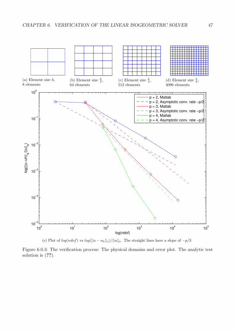
The value of log(||u− uh||a/||u||a should decrease with a factor of −p/3 relative to log(ndof).For p = q = r = 2 and p = q = r = 3 we have plotted these values against each other forh = 1, 1/2, 1/4, 1/8 and 1/16. For p = 4 we have plotted the values for h = 1, 1/2, 1/4, 1/8. For
CHAPTER 6. VERIFICATION OF THE LINEAR ISOGEOMETRIC SOLVER 46
each value of p, we have also drawn a dashed line, showing a slope of −p/3 for easy comparison.Figure (6.0.3a) - (6.0.3d) shows 2D projections of the 3D domains on which we evaluated theerror.
6.0.3 Aspect Ratio
−5
0
5−1
−0.50
0.51
−1
−0.5
0
0.5
1
yx
(a)
−6
−4
−2
0
2
4
6 −1
−0.5
0
0.5
−1500
−1000
−500
0
yx
(b)
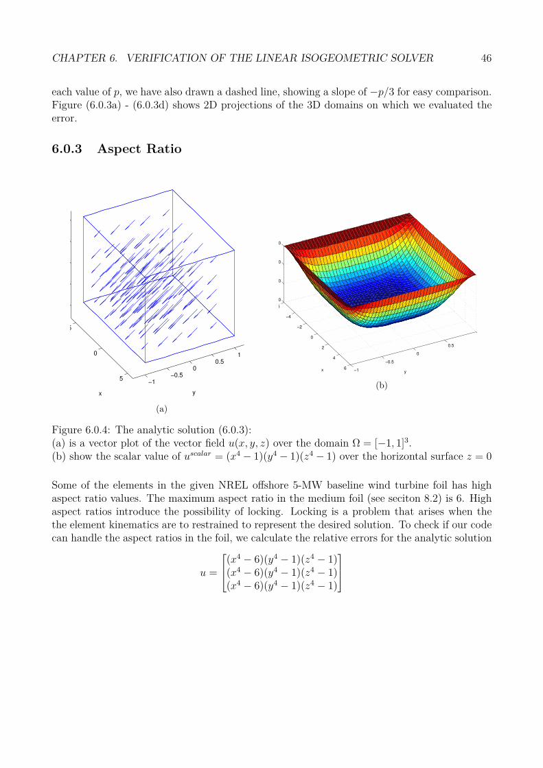
Figure 6.0.4: The analytic solution (6.0.3):(a) is a vector plot of the vector field u(x, y, z) over the domain Ω = [−1, 1]3.(b) show the scalar value of uscalar = (x4 − 1)(y4 − 1)(z4 − 1) over the horizontal surface z = 0
Some of the elements in the given NREL offshore 5-MW baseline wind turbine foil has highaspect ratio values. The maximum aspect ratio in the medium foil (see seciton 8.2) is 6. Highaspect ratios introduce the possibility of locking. Locking is a problem that arises when thethe element kinematics are to restrained to represent the desired solution. To check if our codecan handle the aspect ratios in the foil, we calculate the relative errors for the analytic solution
u =
(x4 − 6)(y4 − 1)(z4 − 1)(x4 − 6)(y4 − 1)(z4 − 1)(x4 − 6)(y4 − 1)(z4 − 1)
CHAPTER 6. VERIFICATION OF THE LINEAR ISOGEOMETRIC SOLVER 47
(a) Element size h,8 elements
(b) Element size h2,
64 elements(c) Element size h
4,
512 elements(d) Element size h
8,
4096 elements
100
101
102
103
104
105
10−5
10−4
10−3
10−2
10−1
100
log(ndof)
log(|
|u−
uh||
a/||u
||a)
p = 2, Matlab
p = 2, Asymptotic conv. rate −p/2
p = 3, Matlab
p = 3, Asymptotic conv. rate −p/2
p = 4, Matlab
p = 4, Asymptotic conv. rate −p/2
(e) Plot of log(ndof) vs log(||u− uh||a)/||u||a. The straight lines have a slope of −p/3
Figure 6.0.3: The verification process: The physical domains and error plot. The analytic testsolution is (??).

CHAPTER 6. VERIFICATION OF THE LINEAR ISOGEOMETRIC SOLVER 48
on the cuboid [−6, 6]× [−1, 1]× [−1, 1]. This result appear to be good, and are shown in figure(6.0.5)

CHAPTER 6. VERIFICATION OF THE LINEAR ISOGEOMETRIC SOLVER 49
(a) Element size h,8 elements
(b) Element size h2,
64 elements
(c) Element size h4,
512 elements(d) Element size h
8,
4096 elements
100
101
102
103
104
105
10−5
10−4
10−3
10−2
10−1
100
log(ndof)
log(|
|u−
uh||
a/||u
||a)
p = 2, Matlab
p = 2, Asymptotic conv. rate −p/2
p = 3, Matlab
p = 3, Asymptotic conv. rate −p/2
p = 4, Matlab
p = 4, Asymptotic conv. rate −p/2
(e) Plot of log(ndof) vs log(||u− uh||a)/||u||a. The straight lines have a slope of −p/3
Figure 6.0.5: The locking problem: The physical domains and error plot for the analytic testsolution (6.0.3).
Chapter 7
Verification of the non-linear solver
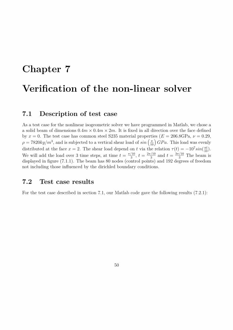
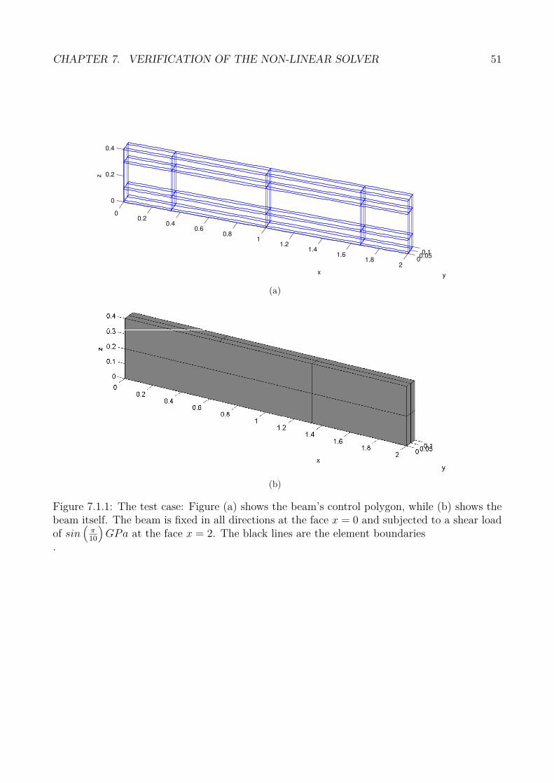
7.1 Description of test case
As a test case for the nonlinear isogeometric solver we have programmed in Matlab, we chose aa solid beam of dimensions 0.4m× 0.4m× 2m. It is fixed in all direction over the face definedby x = 0. The test case has common steel S235 material properties (E = 206.8GPa, ν = 0.29,
ρ = 7820kg/m3, and is subjected to a vertical shear load of sin(
π10
)
GPa. This load was evenly
distributed at the face x = 2. The shear load depend on t via the relation τ(t) = −107sin(πt10
).
We will add the load over 3 time steps, at time t = π/103
, t = 2π/103
and t = 3π/103
The beam isdisplayed in figure (7.1.1). The beam has 80 nodes (control points) and 192 degrees of freedomnot including those influenced by the dirichled boundary conditions.
7.2 Test case results
For the test case described in section 7.1, our Matlab code gave the following results (7.2.1):
50
CHAPTER 7. VERIFICATION OF THE NON-LINEAR SOLVER 51
00.2
0.40.6
0.81
1.21.4
1.61.8
200.050.1
0
0.2
0.4
yx
z
(a)
(b)
Figure 7.1.1: The test case: Figure (a) shows the beam’s control polygon, while (b) shows thebeam itself. The beam is fixed in all directions at the face x = 0 and subjected to a shear loadof sin
(π10
)
GPa at the face x = 2. The black lines are the element boundaries.
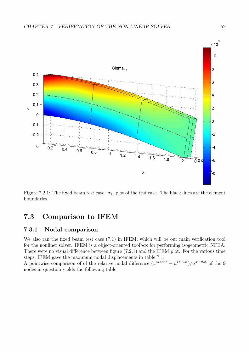
CHAPTER 7. VERIFICATION OF THE NON-LINEAR SOLVER 52
Figure 7.2.1: The fixed beam test case: σ11 plot of the test case. The black lines are the elementboundaries.
7.3 Comparison to IFEM
7.3.1 Nodal comparison
We also ran the fixed beam test case (7.1) in IFEM, which will be our main verification toolfor the nonliner solver. IFEM is a object-oriented toolbox for performing isogeometric NFEA.There were no visual difference between figure (7.2.1) and the IFEM plot. For the various timesteps, IFEM gave the maximum nodal displacements in table 7.1.A pointwise comparison of of the relative nodal difference (uMatlab − uIF EM)/uMatlab of the 9nodes in question yields the following table:

CHAPTER 7. VERIFICATION OF THE NON-LINEAR SOLVER 53
Table 7.1: The fixed beam test case: Maximum nodal displacements, IFEM
Time Step time Max Nodal Displacement
x-direction y-direction z-direction
1 π/103
0.0177454 (node 10) 0.00101751 (node 2) 0.099796 (node 70)
2 2π/103
0.0407524 (node 10) 0.00201773 (node 2) 0.198071 (node 70)
3 3π/103
0.0678808 (node 15) 0.00297953 (node 2) 0.292417 (node 75)
Table 7.2: The fixed beam test case: Relative nodal difference between Matlab and IFEM ofmaximum displacement nodes
Time Step time Relative difference in nodal Dispalcement
x-direction y-direction z-direction
1 π/103
0.0015 (node 10) 2.7597 (node 2) -0.0008 (node 70)
2 2π/103
0.0023 (node 10) 2.7761 (node 2) 0.0002 (node 70)
3 3π/103
0.0034 (node 15) 2.7918 (node 2) 0.0012 (node 75)

CHAPTER 7. VERIFICATION OF THE NON-LINEAR SOLVER 54
7.3.2 Global comparison
For a global comparison of our solver vs IFEM, we have calculated the relative energy norm ofthe difference,
||uMatlab − uIF EM ||a||uMatlab||a
where ||u||a =√
a(u, u). The explicit expression for a(., .) is described in (4.2.3).
Table 7.3: The fixed beam test case: Comparison of the norms ||uMatlab||a and ||uIF EM ||a
Matlab IFEM Difference in norms Relative difference in norms
||uMatlab||a ||uIF EM ||a ||uMatlab − uIF EM ||a||uMatlab−uIF EM ||a
||uMatlab||a
162.38 162.23 1.37 0.0085
7.4 Convergence Rate
Our solver needed 7, 9 and 11 iterations to converge to a tolerance tol = 10−10 for each of thethree time steps. The convergence rate is close quadratic.
Table 7.4: The fixed beam test case: Max nodal displacements, IFEM
Time Step time Max Nodal Displacement
x-direction y-direction z-direction
1 π/103
0.0177454 (node 10) 0.00101751 (node 2) 0.099796 (node 70)
2 2π/103
0.0407524 (node 10) 0.00201773 (node 2) 0.198071 (node 70)
3 3π/103
0.0678808 (node 15) 0.00297953 (node 2) 0.292417 (node 75)
CHAPTER 7. VERIFICATION OF THE NON-LINEAR SOLVER 55
7.5 Discussion
The comparison to IFEM gave a high level of correlation. The low value of the relative differencein a-norm is an indicator that our code is correct. The IFEM result vector we used in thecomparison only had a six digit accuracy for each coefficient in the U solution vector. Theenergy norm is sensitive to changes in the coefficients, and this may have influenced the result.
7.6 Modifications
We implemented some modifications to our code to make it more computational efficient. Weheld the stiffness matrix constand whenever the relative norm was small, and we added aadaptive time step algorithm, that cut ∆t in half whenever the relative norm of the out-of-
balance term ||r(i)||l2||r(0) became to large.

Chapter 8
Results
We will here present the results from the two main problem on which we have used our non-linearisogeometric finite element solver. We will not verify these, but rather present them, in a similar
Figure 8.0.1: Thetwisted bar example inits original configura-tion
way that a mechanical engineer may need in a design phase.
The first result is a case that is sometimes used as a benchmark testin isogeometric analysis settings [2], and is the case of a bar which wetwist in its longitudinal direction. The other result we will presentis the result which has been the aim of nonlinear solver, the NRELoffshore 5-MW baselind wind turbine blade.
8.1 The twisted bar
We have have a bar of dimensions 0.4m·0.4m·5m which is standing invertical z-direction. The bar is illustrated in its original configurationin figure (8.0.1). It is fixed in all directions at the bottom (z = 0) andin z−direction only at the top (z = 5). At the top it is also subjectedto a horisontal shear force that gives a positive torque around thez− axis. We add the shear force subsequently, and see how largerotations we get before the solver diverge. Figure (8.1.1) shows thedevelopment of Von Mieses stress for 8 time steps the our nonlinearsolver managed. The nonlinear solver diverged for time t = t9. Thefinal rotation angle was approximately 140 degrees.
56
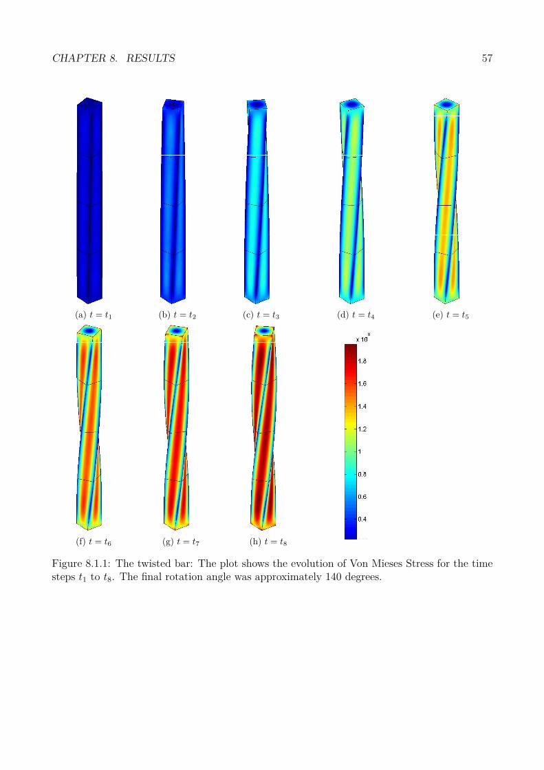
CHAPTER 8. RESULTS 57
(a) t = t1 (b) t = t2 (c) t = t3 (d) t = t4 (e) t = t5
(f) t = t6 (g) t = t7 (h) t = t8
Figure 8.1.1: The twisted bar: The plot shows the evolution of Von Mieses Stress for the timesteps t1 to t8. The final rotation angle was approximately 140 degrees.

CHAPTER 8. RESULTS 58
8.2 The NREL offshore baseline wind
turbine blade
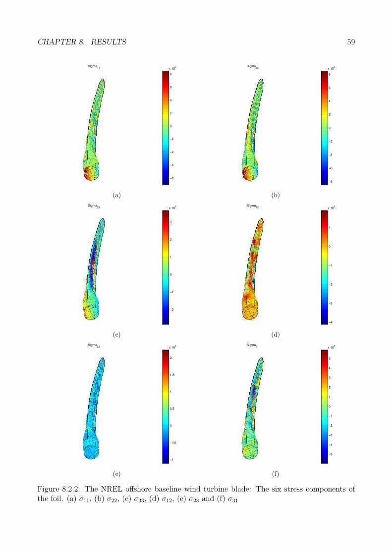
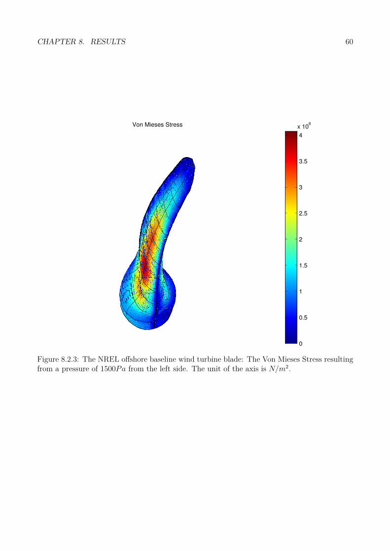
We have applied our nonlinear isogeometric finite element solver on the NREL offshore baselinewind turbine foil to calculate displacement and stress. We chose a load of 1500Pa subjectedto the foil as pressure on the flat side of the wing. If we assume that all the wind moleculestransfer their entire linear momentum to the foil, a square meter of the foil will stop a volumeof V = [windspeed] · 1m2 · 1s air every second. From this, simple hand calculations yield thatfor a wind speed of 35m/s, the pressure of the foil would be 1500Pa. We have tested threedifferent discretizations of various size, but we will only display the results from most refinedmodel here. This discretization has 280 nodes (control points), and 780 degrees of freedom.Figure (8.2.1) shows some of the rotor’s geometrical properties. Figure 8.2.2 shows plots of thesix unique components of the stress tensor, and figure (8.2.3) the shows the Von Mieses Stress.
(a)
(b)
(c)
Figure 8.2.1: The NREL offshore baseline wind turbine blade’s origial configuration. (a): Thecontrol polygon of the foil, (b): The wind foil with true proposions, (c): The wind foil seenfrom top down, viewing the foil profiles
CHAPTER 8. RESULTS 59
Sigma11
−8
−6
−4
−2
0
2
4
6
8
x 105
(a)
Sigma22
−8
−6
−4
−2
0
2
4
6
8
x 105
(b)
Sigma33
−2
−1
0
1
2
3
x 106
(c)
Sigma12
−4
−3
−2
−1
0
1
x 105
(d)
Sigma23
−1
−0.5
0
0.5
1
1.5
2
x 106
(e)
Sigma31
−5
−4
−3
−2
−1
0
1
2
3
4
5
x 105
(f)
Figure 8.2.2: The NREL offshore baseline wind turbine blade: The six stress components ofthe foil. (a) σ11, (b) σ22, (c) σ33, (d) σ12, (e) σ23 and (f) σ31
CHAPTER 8. RESULTS 60
Von Mieses Stress
0
0.5
1
1.5
2
2.5
3
3.5
4
x 106
Figure 8.2.3: The NREL offshore baseline wind turbine blade: The Von Mieses Stress resultingfrom a pressure of 1500Pa from the left side. The unit of the axis is N/m2.

CHAPTER 8. RESULTS 61
8.2.1 Physical Interpretation
The highest value of Von Mieses Stress for the design load is below the yield strength of thegiven material. Thus, the foil distortion is within the elastic range of the design.

Chapter 9
Concluding remarks
We have programmed a linear and a nonlinear isogeometric finite element solver in Matlab codefor the elasticity problem. For code verification, the linear Matlab solver code was compared totest problems where we had analytic solutions.The nonlinear solver was compared to the IFEMsoftware, where it correlated well. The nonlinear solver was applied to a twisted bar case andthe wind turbine foil of the NREL offshore 5-MW baseline wind turbine. The analytical resultswere visualised in distortion plots and Von Mieses stress plots.
62

Appendices
63
Appendix A
Notation
A.1 Basis functions
NI : A scalar basis function.I: The index of a scalar basis function, I = (i− 1)mo + (j − 1)o + kNI : A vector basis function.
NI =
NI
[
1 0 0]T
if I = 1, 4, 7, . . .
NI
[
0 1 0]T
if I = 2, 5, 8, . . .
NI
[
0 0 1]T
if I = 3, 6, 9, . . .
The matrix N is defined as
N = [N1, N2, ..., N3lmo]
A.2 Nonlinear sections
Left super and sub indices: timeconfigurationR(iteration numer)
t: Pseudo time. Influence the system via the external load vector, which increase with time.tΩ: Domain (configuration) at (pseudo-)time t.tx is the x-coordiate refered to configuration tΩ.Xi = 0xi.U : The coefficient vector. The coefficients is the displacement in the controlpoints in the ap-propriate direction.t+∆t
tE: Almansi strain
64

APPENDIX A. NOTATION 65
t0E: Green strain.
0E : = t+∆t0E −
t0E.
t+∆tσij: Cauchy stress at time t + ∆t.t+∆t
tSij: 2 PK stress tensor induced from the displacement relative to tΩ, (i.e induced fromt+∆t
tu) .t+∆tR: Externally applied force.t+∆tR: Virtual work due from the external forces.t+∆t
tEij = t+∆ttǫij + t+∆t
tβijt+∆t
tǫij: linear part of the GL strain.t+∆t
tβij: nonlinear part of the GL strain

Appendix B
Notation
B.0.1 Voigt notation
ǫ =
ǫ11
ǫ22
ǫ33
ǫ12
ǫ23
ǫ31
, σ =
σ11
σ22
σ33
σ12
σ23
σ31
, v =
v1
v2
v3
∈ V 3, f =
f1
f2
f3
σ = Cǫ =E
1− ν2
1 ν 0ν 1 00 0 1−ν
2
ǫ11
ǫ22
ǫ12
When we write something in matrix form, we will consistently use Voight notationSections refereres til slik: sec 1.3ligninger refereres slik: (4.1)Every time I introduce a new variable I will write it here:d: The dimension of our physical domain, Ω ⊂ R
d
Γ: Grensen av Ω,dvs jeg bruker dette istedenfor ∂Ω. Jeg gidder ikke skrive den i bold.Hk(Ω): Sobolev space. Hk(Ω) = f ∈ L2(Ω) : Dαf ∈ L2(Ω)∀α : |α| ≤ k
Dαf = ∂|α|
∂xα11 ∂x
α22 ∂x
α33
, |α| =∑
i αi (in three dimensions).
u =Nbf∑
I=1
uINI
= u1
[
S1
0
]
+ u2
[
0S1
]
+ u3
[
S2
0
]
+ u4
[
0S2
]
+ ... + uNbf −1
[
Snm
0
]
+ uNbf
[
0Snm
]
66

Appendix C
Linear Isogeometric Finite ElementSover
C.1 Algorithms for assemling the stiffness matrix
Mathematically, we wish to calculate
AJ,I =∫
Ωǫ(NJ)T Cǫ(NI) dΩ
=nk∑
e=1
∫
Ωeǫ(NJ)T Cǫ(NI) dΩ
=nk∑
e=1
ak(NI , NJ)
We do this via the loop:
....................................for Ωe = Ω1 . . . Ωnk
..........................................for all I ∈ IΩe
................................................for all J ∈ IΩe
......................................................AJ,I = AJ,I + ak(NI , NJ)
................................................end
..........................................end
....................................end
where IΩe is the set of those basisfunctions that will not be influenced by the homogeneousdirichlet conditions.
67
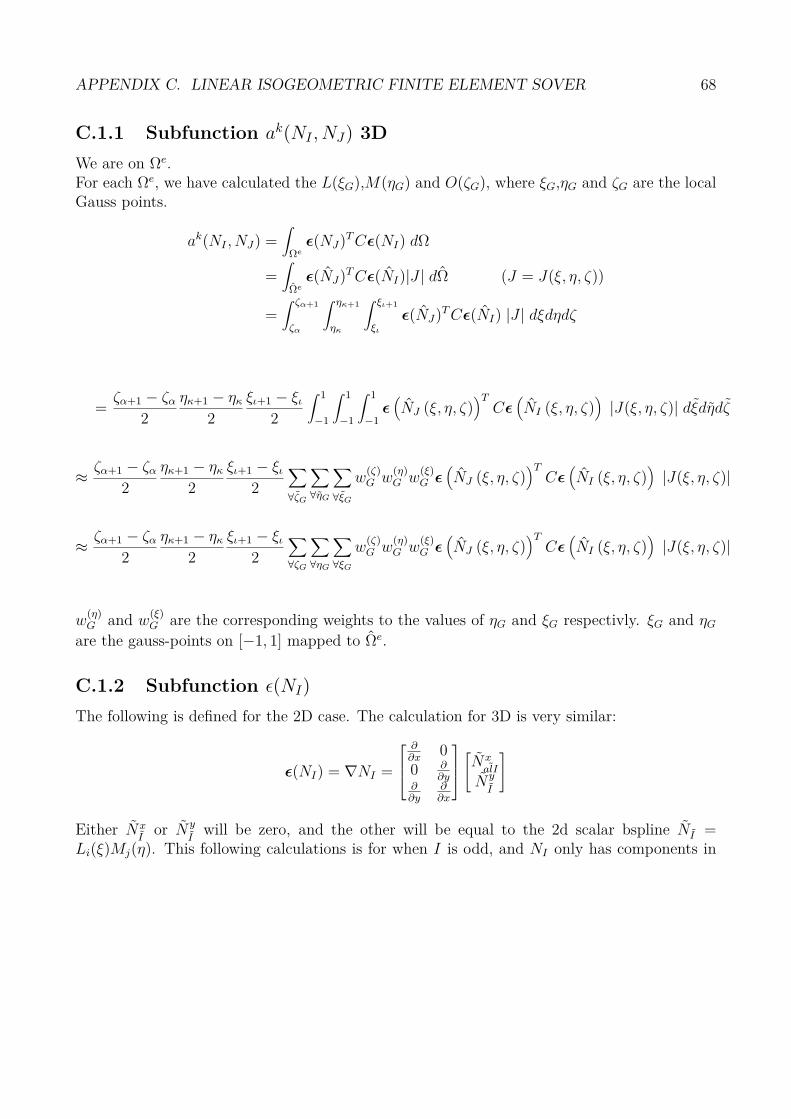
APPENDIX C. LINEAR ISOGEOMETRIC FINITE ELEMENT SOVER 68
C.1.1 Subfunction ak(NI , NJ) 3D
We are on Ωe.For each Ωe, we have calculated the L(ξG),M(ηG) and O(ζG), where ξG,ηG and ζG are the localGauss points.
ak(NI , NJ) =∫
Ωeǫ(NJ)T Cǫ(NI) dΩ
=∫
Ωeǫ(NJ)T Cǫ(NI)|J | dΩ (J = J(ξ, η, ζ))
=∫ ζα+1
ζα
∫ ηκ+1
ηκ
∫ ξι+1
ξι
ǫ(NJ)T Cǫ(NI) |J | dξdηdζ
=ζα+1 − ζα
2
ηκ+1 − ηκ
2
ξι+1 − ξι
2
∫ 1
−1
∫ 1
−1
∫ 1
−1ǫ(
NJ (ξ, η, ζ))T
Cǫ(
NI (ξ, η, ζ))
|J(ξ, η, ζ)| dξdηdζ
≈ζα+1 − ζα
2
ηκ+1 − ηκ
2
ξι+1 − ξι
2
∑
∀ζG
∑
∀ηG
∑
∀ξG
w(ζ)G w
(η)G w
(ξ)G ǫ
(
NJ (ξ, η, ζ))T
Cǫ(
NI (ξ, η, ζ))
|J(ξ, η, ζ)|
≈ζα+1 − ζα
2
ηκ+1 − ηκ
2
ξι+1 − ξι
2
∑
∀ζG
∑
∀ηG
∑
∀ξG
w(ζ)G w
(η)G w
(ξ)G ǫ
(
NJ (ξ, η, ζ))T
Cǫ(
NI (ξ, η, ζ))
|J(ξ, η, ζ)|
w(η)G and w
(ξ)G are the corresponding weights to the values of ηG and ξG respectivly. ξG and ηG
are the gauss-points on [−1, 1] mapped to Ωe.
C.1.2 Subfunction ǫ(NI)
The following is defined for the 2D case. The calculation for 3D is very similar:
ǫ(NI) = ∇NI =
∂∂x
00 ∂
∂y∂
∂y∂
∂x
[
NxalI
Ny
I
]
Either NxI
or Ny
Iwill be zero, and the other will be equal to the 2d scalar bspline NI =
Li(ξ)Mj(η). This following calculations is for when I is odd, and NI only has components in
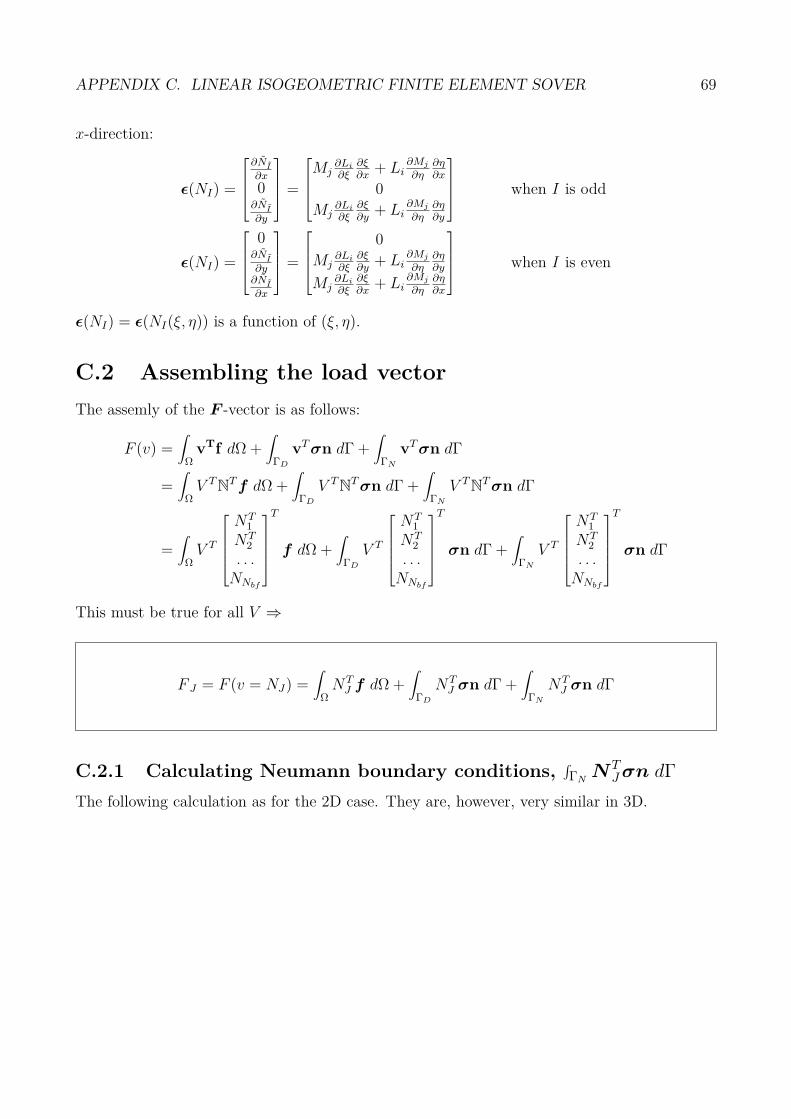
APPENDIX C. LINEAR ISOGEOMETRIC FINITE ELEMENT SOVER 69
x-direction:
ǫ(NI) =
∂NI
∂x
0∂NI
∂y
=
Mj∂Li
∂ξ∂ξ∂x
+ Li∂Mj
∂η∂η∂x
0
Mj∂Li
∂ξ∂ξ∂y
+ Li∂Mj
∂η∂η∂y
when I is odd
ǫ(NI) =
0∂NI
∂y∂NI
∂x
=
0
Mj∂Li
∂ξ∂ξ∂y
+ Li∂Mj
∂η∂η∂y
Mj∂Li
∂ξ∂ξ∂x
+ Li∂Mj
∂η∂η∂x
when I is even
ǫ(NI) = ǫ(NI(ξ, η)) is a function of (ξ, η).
C.2 Assembling the load vector
The assemly of the F -vector is as follows:
F (v) =∫
ΩvTf dΩ +
∫
ΓD
vT σn dΓ +∫
ΓN
vT σn dΓ
=∫
ΩV T
NT f dΩ +
∫
ΓD
V TN
T σn dΓ +∫
ΓN
V TN
T σn dΓ
=∫
ΩV T
NT1
NT2
. . .NNbf
T
f dΩ +∫
ΓD
V T
NT1
NT2
. . .NNbf
T
σn dΓ +∫
ΓN
V T
NT1
NT2
. . .NNbf
T
σn dΓ
This must be true for all V ⇒
F J = F (v = NJ) =∫
ΩNT
J f dΩ +∫
ΓD
NTJ σn dΓ +
∫
ΓN
NTJ σn dΓ
C.2.1 Calculating Neumann boundary conditions,∫
ΓNNT
J σn dΓ
The following calculation as for the 2D case. They are, however, very similar in 3D.
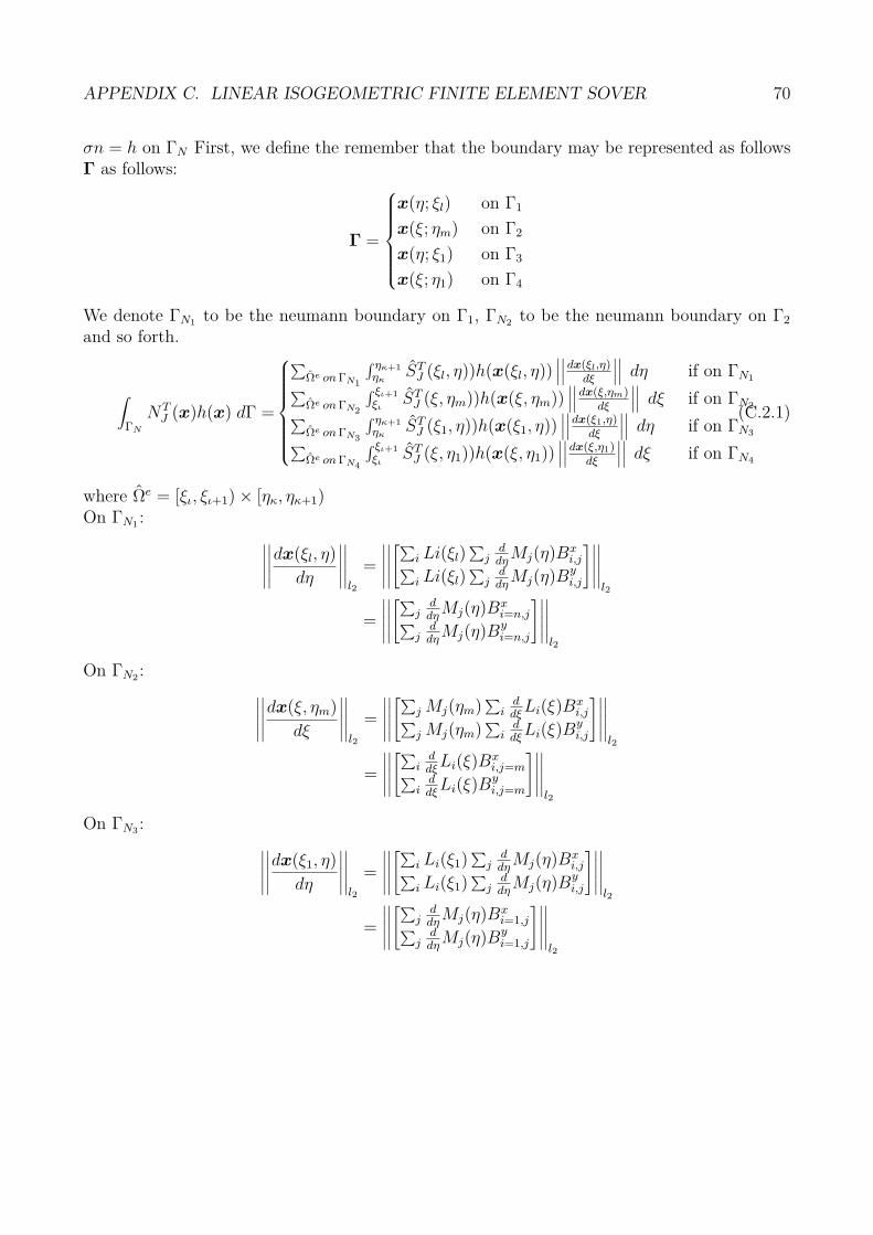
APPENDIX C. LINEAR ISOGEOMETRIC FINITE ELEMENT SOVER 70
σn = h on ΓN First, we define the remember that the boundary may be represented as followsΓ as follows:
Γ =
x(η; ξl) on Γ1
x(ξ; ηm) on Γ2
x(η; ξ1) on Γ3
x(ξ; η1) on Γ4
We denote ΓN1 to be the neumann boundary on Γ1, ΓN2 to be the neumann boundary on Γ2
and so forth.
∫
ΓN
NTJ (x)h(x) dΓ =
∑
Ωe on ΓN1
∫ ηκ+1ηκ
STJ (ξl, η))h(x(ξl, η))
∣∣∣
∣∣∣
dx(ξl,η)dξ
∣∣∣
∣∣∣ dη if on ΓN1
∑
Ωe on ΓN2
∫ ξι+1
ξιST
J (ξ, ηm))h(x(ξ, ηm))∣∣∣
∣∣∣
dx(ξ,ηm)dξ
∣∣∣
∣∣∣ dξ if on ΓN2
∑
Ωe on ΓN3
∫ ηκ+1ηκ
STJ (ξ1, η))h(x(ξ1, η))
∣∣∣
∣∣∣
dx(ξ1,η)dξ
∣∣∣
∣∣∣ dη if on ΓN3
∑
Ωe on ΓN4
∫ ξι+1
ξιST
J (ξ, η1))h(x(ξ, η1))∣∣∣
∣∣∣
dx(ξ,η1)dξ
∣∣∣
∣∣∣ dξ if on ΓN4
(C.2.1)
where Ωe = [ξι, ξι+1)× [ηκ, ηκ+1)On ΓN1 :
∣∣∣∣∣
∣∣∣∣∣
dx(ξl, η)
dη
∣∣∣∣∣
∣∣∣∣∣l2
=
∣∣∣∣∣
∣∣∣∣∣
[∑
i Li(ξl)∑
jd
dηMj(η)Bx
i,j∑
i Li(ξl)∑
jd
dηMj(η)By
i,j
]∣∣∣∣∣
∣∣∣∣∣l2
=
∣∣∣∣∣
∣∣∣∣∣
[∑
jd
dηMj(η)Bx
i=n,j∑
jd
dηMj(η)By
i=n,j
]∣∣∣∣∣
∣∣∣∣∣l2
On ΓN2 :
∣∣∣∣∣
∣∣∣∣∣
dx(ξ, ηm)
dξ
∣∣∣∣∣
∣∣∣∣∣l2
=
∣∣∣∣∣
∣∣∣∣∣
[∑
j Mj(ηm)∑
iddξ
Li(ξ)Bxi,j
∑
j Mj(ηm)∑
iddξ
Li(ξ)Byi,j
]∣∣∣∣∣
∣∣∣∣∣l2
=
∣∣∣∣∣
∣∣∣∣∣
[∑
iddξ
Li(ξ)Bxi,j=m
∑
iddξ
Li(ξ)Byi,j=m
]∣∣∣∣∣
∣∣∣∣∣l2
On ΓN3 :
∣∣∣∣∣
∣∣∣∣∣
dx(ξ1, η)
dη
∣∣∣∣∣
∣∣∣∣∣l2
=
∣∣∣∣∣
∣∣∣∣∣
[∑
i Li(ξ1)∑
jd
dηMj(η)Bx
i,j∑
i Li(ξ1)∑
jd
dηMj(η)By
i,j
]∣∣∣∣∣
∣∣∣∣∣l2
=
∣∣∣∣∣
∣∣∣∣∣
[∑
jd
dηMj(η)Bx
i=1,j∑
jd
dηMj(η)By
i=1,j
]∣∣∣∣∣
∣∣∣∣∣l2

APPENDIX C. LINEAR ISOGEOMETRIC FINITE ELEMENT SOVER 71
On ΓN4
∣∣∣∣∣
∣∣∣∣∣
dx(ξ, η1)
dξ
∣∣∣∣∣
∣∣∣∣∣l2
=
∣∣∣∣∣
∣∣∣∣∣
[∑
j Mj(η1)∑
iddξ
Li(ξ)Bxi,j
∑
j Mj(η1)∑
iddξ
Li(ξ)Byi,j
]∣∣∣∣∣
∣∣∣∣∣l2
=
∣∣∣∣∣
∣∣∣∣∣
[∑
iddξ
Li(ξ)Bxi,j=1
∑
iddξ
Li(ξ)Byi,j=1
]∣∣∣∣∣
∣∣∣∣∣l2
We use gauss integration to calculate (C.2.1):We can skip the first summation sign since Mj(ηm) is different from zero only in j = m.
For ΓN1
∫
ΓN1
NTJ (x)h(x) dΓ =
∑
Ωe on ΓN1
∫ ηκ+1
ηκ
STJ (ξl, η))h(x(ξl, η))
∣∣∣∣∣
∣∣∣∣∣
dx(ξl, η)
dξ
∣∣∣∣∣
∣∣∣∣∣
dη
=∑
Ωe on ΓN1
∫ ηκ+1
ηκ
f(η) dη
=∑
Ωe on ΓN1
ηκ+1 − ηκ
2
∑
ηG
w(η)f(ηG)
f(η) = STJ (ξl, η))h(x(ξl, η))
∣∣∣∣∣
∣∣∣∣∣
dx(ξl, η)
dξ
∣∣∣∣∣
∣∣∣∣∣
= ˆSJ(ξl, η))
[
J == oddJ == even
]T
h(x(ξl, η))
∣∣∣∣∣
∣∣∣∣∣
dx(ξl, η)
dξ
∣∣∣∣∣
∣∣∣∣∣
f(ηG) = Li(ξl)︸ ︷︷ ︸
=δin
Mj(ηG)
[
J == oddJ == even
]T
h(x(ξl, ηG︸ ︷︷ ︸
evaluert
))
∣∣∣∣∣
∣∣∣∣∣
dx(ξl, ηG)
dξ
∣∣∣∣∣
∣∣∣∣∣
︸ ︷︷ ︸
evaluertiηG
where (i, j) corresponds to JEvaluation x(ξl, ηG):
x(ξ1, ηG) =
[∑
i Li(ξ1)∑
j Mj(ηG)Bxi,j
∑
i Li(ξ1)∑
j Mj(ηG)Byi,j
]
=
[∑
j Mj(ηG)Bxi=1,j
∑
j Mj(ηG)Byi=1,j
]
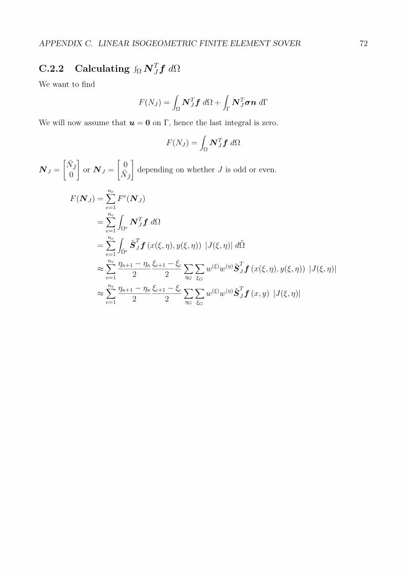
APPENDIX C. LINEAR ISOGEOMETRIC FINITE ELEMENT SOVER 72
C.2.2 Calculating∫
Ω NTJ f dΩ
We want to find
F (NJ) =∫
ΩNT
J f dΩ +∫
ΓNT
J σn dΓ
We will now assume that u = 0 on Γ, hence the last integral is zero.
F (NJ) =∫
ΩNT
J f dΩ
NJ =
[
NJ
0
]
or NJ =
[
0NJ
]
depending on whether J is odd or even.
F (NJ) =ne∑
e=1
F e(NJ)
=ne∑
e=1
∫
ΩeNT
J f dΩ
=ne∑
e=1
∫
ΩeS
T
J f (x(ξ, η), y(ξ, η)) |J(ξ, η)| dΩ
≈ne∑
e=1
ηκ+1 − ηκ
2
ξι+1 − ξι
2
∑
ηG
∑
ξG
w(ξ)w(η)ST
J f (x(ξ, η), y(ξ, η)) |J(ξ, η)|
≈ne∑
e=1
ηκ+1 − ηκ
2
ξι+1 − ξι
2
∑
ηG
∑
ξG
w(ξ)w(η)ST
J f (x, y) |J(ξ, η)|

Appendix D
Impementation details for thenonlinear solver
D.1 How to calculate ttGI J
ttGIJ = I(3×3)
∫
tΩtN I,i
tσij tN J ,jtdΩ
= I(3×3)nel∑
e=1
∫
tΩetN I,i
tσij tN J ,jtdΩe
= I(3×3)nel∑
e=1
∫
tΩe
tN I,itσij tN J ,j|J |
tdΩe
= I(3×3)nel∑
e=1
ζα+1 − ζα
2
βκ+1 − βκ
2
ξι+1 − ξι
2
∑
ξG
∑
βG
∑
ζG
w(ξ)w(β)w(ζ)(
tN I,itσij tN J ,j
)
|J |
(D.1.1)
D.1.1 Practical Implementation
A matlab script, calcKG has been made for the purpose of calculation KG. It follows an algo-rithm that is mathematical equivalent to equation (5.2.6) and (D.1.1), and is given below:
for all elements Ωe, e = 1..., nel.......for I = 1, 2, ..., lmo.............for J = 1, 2, ..., I...................Calculate the gauss-sum GS (D.1.2).
73

APPENDIX D. IMPEMENTATION DETAILS FOR THE NONLINEAR SOLVER 74
........................Insert GS into KG at:
........................KG(Ix(I),Jx(J)) ← GS
........................KG(Iy(I),Jy(J)) ← GS
........................KG(Iz(I),Jz(J)) ← GS
........................KG(Jx(I),Ix(J)) ← GS
........................KG(Jy(I),Iy(J)) ← GS
........................KG(Jz(I),Iz(J)) ← GS
..................end
............end
......endend
where Ix(I), Iy(I) and Iz(I) relate through : Ix = 3(I − 1) + 1, Iy = 3(I − 1) + 2 and Iz = 3I.
We have here used the symmetric property of G, GIJ = GJ I .
GS =
ζα+1 − ζα
2
βκ+1 − βκ
2
ξι+1 − ξι
2
∑
ξG
∑
βG
∑
ζG
w(ξ)w(β)w(ζ)(
tN I,itσij tN J ,j
)
|J |
(D.1.2)
D.2 Calculation of t+∆tt+∆tF
ttF =
∫
tΩBT tσ tdΩ
=∫
tΩ(∇ tN)T tσ tdΩ

APPENDIX D. IMPEMENTATION DETAILS FOR THE NONLINEAR SOLVER 75
t0ǫ = 1
2( t
0ui,j + t0uj,i) + 1
2( t
0uk,it0uk,j) (from MIT 5-5, transpacency 5-3).
ttF =
∫
tΩ(∇ tN)T tσ tdΩ
=nel∑
e=1
∫
tΩe(∇ tN)T tσ tdΩ
=nel∑
e=1
∫
tΩe
(∇ tN)T tσ|J | tdΩ
=nel∑
e=1
ζα+1 − ζα
2
βκ+1 − βκ
2
ξι+1 − ξι
2
∑
ξG
∑
βG
∑
ζG
wξwβwζ(∇ tN)T tσ|J |
where tσ is given by (3.1.1)
D.3 Finding nonlinear GL strain, t0E
Define tN.,i = ∂ tN
∂ txi(according to standard matrix derivative rules (ref wikipedia(?)).
t0ǫij =
1
2
(t0ui,j + t
0uj,i
)
+1
2
(t0uk,i
t0uk,j
)
=1
2
(
( tN.,j)(i,:) + ( tN.,i)(j,:))
)
U +1
2
(
( tN.,i)(k,:) U) (
( tN.,j)(k,:) U)
=1
2
(
( tN.,j)(i,:) + ( tN.,i)(j,:))
)
U +1
2(( tN.,i) U)T (( tN.,j) U)
D.4 Update Control Polygon
Update tΩ to contain the deformation from t+∆tU (k).Do this by updating the control polygon,
tP =
tP xI=1
tP xI=2
tP xI=3
tP y
I=1tP y
I=2tP y
I=3. . .
tP zI=1
tP zI=2
tP zI=3
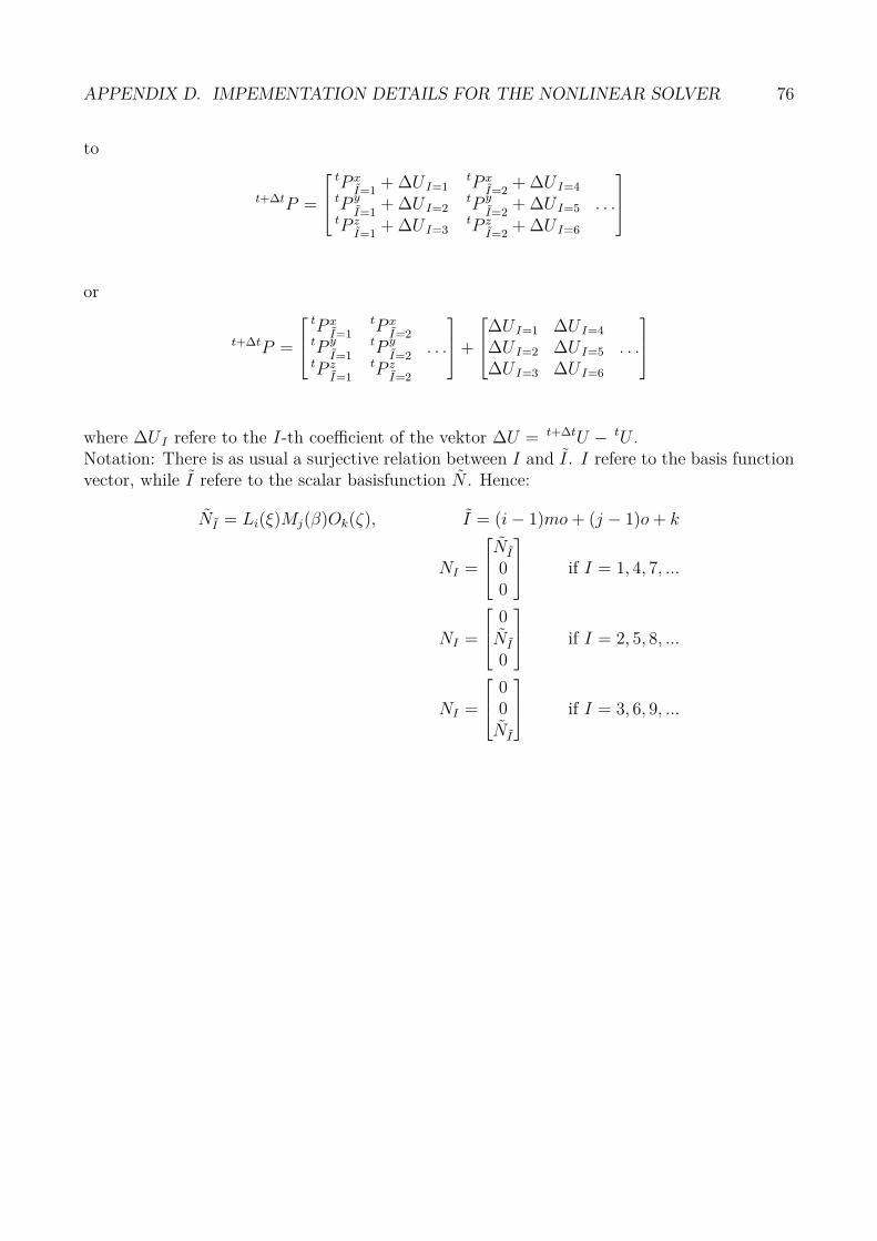
APPENDIX D. IMPEMENTATION DETAILS FOR THE NONLINEAR SOLVER 76
to
t+∆tP =
tP xI=1
+ ∆U I=1tP x
I=2+ ∆U I=4
tP y
I=1+ ∆U I=2
tP y
I=2+ ∆U I=5 . . .
tP zI=1
+ ∆U I=3tP z
I=2+ ∆U I=6
or
t+∆tP =
tP xI=1
tP xI=2
tP y
I=1tP y
I=2. . .
tP zI=1
tP zI=2
+
∆U I=1 ∆U I=4
∆U I=2 ∆U I=5 . . .∆U I=3 ∆U I=6
where ∆U I refere to the I-th coefficient of the vektor ∆U = t+∆tU − tU .Notation: There is as usual a surjective relation between I and I. I refere to the basis functionvector, while I refere to the scalar basisfunction N . Hence:
NI = Li(ξ)Mj(β)Ok(ζ), I = (i− 1)mo + (j − 1)o + k
NI =
NI
00
if I = 1, 4, 7, ...
NI =
0NI
0
if I = 2, 5, 8, ...
NI =
00
NI
if I = 3, 6, 9, ...

Appendix E
Program Structure
We will here give a brief overview of the program structure of our code. We have programmedthe programs from scratch in Matlab, and we will here briefly display how the most importantprograms relate.
77

APPENDIX E. PROGRAM STRUCTURE 78
main.m
input file(Generates
or loadsthe geome-try model)
NonlinearAlgorithmneste linjeog neste
calc KM calc KG calc R calc F UpdateControlPolygon
Output (post-processing)
calc stress inx-,y-
and z-direciton
Plotresults

Chapter 10
Bibliography
79

Bibliography
[1] Klaus-Jürgen Bathe. Finite Element Procedures in Engineering Analysis. 1982.
[2] Nils Zander Yuri Bazilevs Alexander Düster Ernst Rank Dominik Schillinger, Mar-tin Ruess. Small and large deformation analysis with the p- and b-spline versions ofthe finite cell method. Springer-Verlag, 2012.
[3] Amos Eaton. The finite element method. http://www.cs.rpi.edu/ flaherje/pdf/fea7.pdf.
[4] Jacob Fish. A First Course In Finite Elements. Wiley, 2007.
[5] T. J. R. Hughes, J. A. Cottrell, and Y. Bazilevs. Isogeometric analysis cad, finite elements,nurbs, exact geometry and mesh refinement. Computer Methods in Applied Mechanics andEngineering, 194:4135–4195, 2005.
[6] T. J. R. Hughes, J. A. Cottrell, and Y. Bazilevs. Isogeometric analysis: Toward unificationof cad and fea. Wiley, 2009.
[7] T.J.R. Hughes, A. Reali, and G. Sangalli. Effmethod quadrature for nurbs-based isogeo-metric analysis. Computer Methods in Applied Mechanics and Engineering, 199:249–333,2010.
[8] Vladimir Ivanco. Nonlinear finite element analysis, 2011.
[9] I. V. Kerlow. The art of 3d computer animation and effects. Wiley, 2004.
[10] Tom Lyche and Knut Morken. Spline Methods. Universitetet i Oslo, 2011.
[11] Kjell Magne Mathisen. Fe formulation of quasi-static geometrically non-linear solid me-chanics.
[12] Kjell Magne Mathisen. Formulation of Geometrically Nonlinear FE.
[13] L.A.M Mendes and L.M.S.S. Castro. Hybrid-mixed stress finite element models in elasto-plastic analysis. Finite Element in Analysis and Designe, 45(12):863–875, 2009.
80

BIBLIOGRAPHY 81
[14] Takashi Nomura. Prediction of large-scale wind field over a complex terrain by finiteelement method. Journal of Wind Engineering and Industrial Aerodynamics, 67&68, 1997.
[15] Alfio Quarteroni, Tom Hou, Claude Le Bris, Anthony T. Patera, and Enrique Zuazua.Numerical Models for Differential Problems. Springer, 2009.
[16] Jackson Cothren Snow L. Winters Robert G. Sullivan, Leslie B. Kirchler. Preliminaryassessment of offshore wind turbine visibility and visual impact threshold distances. 2012.
[17] D. F. Rogers. An introduction to nurbs with historical perspective. Academic Press, 2001.
[18] Brian Moran Ted Belytschko, Wing Kam Lie. Nonlinear Finite Elements for Continuaand Structures. Wiley, 2000.
[19] B. Xiao and P. Weng. Inanalysis analysis of the electromagnetical, thermal, fluid flowfields in a tokamak. Fusion Engineering and Design, 81(8-14):1549–1554, 2006.
[20] Y. Zhang T. J. R. Hughes Y. Bazilevs, V. M. Calo. Isogeometric fluid-structure interactionanalysis with applications to arterial blood flow.
[21] Cui Junzhi Mang Yuan, Yong. Computational structural engineering: Proceedings of theinternational symposium on computational structural engineering. 2009.
[22] Tao Tang Zhilin Li, Zhonghua Qiao. Numerical Solutions of Partial Differential Equa-tionsŰ An Introduction to Finite Difference and Finite Element Methods. 2012.