isogeometric finite element analysis of nonlinear … › ... › file ›...
TRANSCRIPT

Isogeometric Finite Element Analysisof Nonlinear Structural Vibrations
Oliver Weeger
Vom Fachbereich Mathematik der Technischen Universitat Kaiserslauternzur Verleihung des akademischen Grades
Doktor der Naturwissenschaften(Doctor rerum naturalium, Dr. rer. nat.)
genehmigte Dissertation.
1. Gutachter: Prof. Dr. Bernd Simeon (Technische Universitat Kaiserslautern)2. Gutachter: Prof. Dr. Carlo Lovadina (Universita degli studi di Pavia)Datum der Disputation: 17. April 2015
D 386

ii

Zusammenfassung
In dieser Arbeit stellen wir eine neuartige Methode fur die nichtlineare Frequenzanalysevon angeregten mechanischen Schwingungen vor. Zur effizienten Ortsdiskretisierung derpartiellen Differentialgleichungen der nichtlinearen Kontinuumsmechanik wenden wir dasPrinzip der isogeometrischen Analyse an. Die isogeometrische Finite Elemente Methodebietet im Vergleich zu klassischen Finiten Elemente-Diskretisierungen zahlreiche Vorteile,insbesondere eine exakte Geometriedarstellung und hohere Genauigkeit der numerischenApproximationen mittels Spline-Funktionen. Anschließend verwenden wir die HarmonicBalance Methode zur Berechnung der nichtlinearen Schwingungsantwort bei periodischenexternen Anregungen. Dabei wird die Losung des aus der Ortsdiskretisierung resultie-renden, nichtlinearen gewohnlichen Differentialgleichungssystems im Frequenzraum alsabgeschnittene Fourierreihe entwickelt. Um eine effektive Anwendung der Methode aufgroße Systeme im Rahmen von industriellen Problemen zu ermoglichen, ist eine Modell-reduktion der Ortsdiskretisierung der Bewegungsgleichung notwendig. Dazu schlagen wireine modale Projektionsmethode vor, die mit modalen Ableitungen und damit Informati-onen zweiter Ordnung erweitert wird. Wir untersuchen das Prinzip der modalen Ablei-tungen theoretisch und demonstrieren anhand numerischer Beispiele die Anwendbarkeitund Genauigkeit der Reduktionsmethode bei der nichtlinearen Frequenzanalyse. Außer-dem erweitern wir die nichtlineare Vibrationsanalyse mittels gemischter isogeometrischerMethoden auf inkompressible Elastizitat.
iii

iv

Abstract
In this thesis we present a new method for nonlinear frequency response analysis of me-chanical vibrations. For an efficient spatial discretization of nonlinear partial differentialequations of continuum mechanics we employ the concept of isogeometric analysis. Isogeo-metric finite element methods have already been shown to possess advantages over clas-sical finite element discretizations in terms of exact geometry representation and higheraccuracy of numerical approximations using spline functions. For computing nonlinearfrequency response to periodic external excitations, we rely on the well-established har-monic balance method. It expands the solution of the nonlinear ordinary differentialequation system resulting from spatial discretization as a truncated Fourier series in thefrequency domain. A fundamental aspect for enabling large-scale and industrial applica-tion of the method is model order reduction of the spatial discretization of the equationof motion. Therefore we propose the utilization of a modal projection method enhancedwith modal derivatives, providing second-order information. We investigate the conceptof modal derivatives theoretically and using computational examples we demonstrate theapplicability and accuracy of the reduction method for nonlinear static computations andvibration analysis. Furthermore, we extend nonlinear vibration analysis to incompressibleelasticity using isogeometric mixed finite element methods.
v

vi

Acknowledgements
Over the last years many people have been supporting me in the course of preparing thisthesis and I would like to acknowledge their kind efforts and assistance.
First of all, I would like to express my gratitude towards my supervisor Prof Dr BerndSimeon for guiding my research over the last five years, first a as diploma student atTU Munchen and then as a PhD candidate at TU Kaiserslautern. I appreciate that heleft a lot of freedom for me to pursue my own ideas, set the right direction when it wasnecessary and contributed valuable advice.
I am also very grateful to Dr Utz Wever, who has been my advisor at Siemens formany years. He supported my work in various ways and was always available for fruitfuldiscussions. Furthermore I want to thank Dr Stefan Boschert for leading our TERRIFICproject activities at Siemens and his profound advice.
I also want to thank the research group heads at Siemens Corporate Technology, DrEfrossini Tsouchnika and Roland Rosen, who gave me the chance to pursue my PhDproject in an industrial environment and contributed the funding for my research ac-tivities. For the pleasant and inspiring working environment, I would like to thank allmy colleagues at Siemens, in particular Dr Meinhard Paffrath, Dr Dominic Kohler andDr Yayun Zhou for their company and support. My thanks also goes to all other PhDstudents at Siemens CT and StuNet for discussions, lunches and leisure activities.
I am indebted to Prof Dr Carlo Lovadina for giving me the chance to spend a two-monthresearch visit at the University of Pavia and the excellent cooperation we had there. DrNicola Cavallini deserves my special thanks for the great collaboration, his dedication toour work and his manifold support. I also want to thank all the colleagues and friends Imet in Pavia for the joyful time we had together.
For the close collaboration, fruitful discussions and her support, I deeply want to expressmy gratitude towards my colleague Daniela Fußeder. At TU Kaiserslautern I furthermorewant to thank Dr Anh-Vu Vuong and Anmol Goyal for their cooperation.
It was a great pleasure to work with many colleagues from all over Europe, who wereinvolved in the “TERRIFIC” EU project. I want to thank them for the collaboration andenjoyable project meetings. Special thanks goes to the group of Prof Dr Bert Juttler atJKU Linz and Dr Vibeke Skytt from SINTEF in Oslo, who supported my work with theirmulti-patch parameterizations.
For the balancing distraction, relaxation and fun we had together in the last years, Iam very thankful to all my friends.
vii

In the end I would also like to thank the most important person in my life, my girlfriendSerene, who has been giving me so much encouragement and joy over all the years. Deepestthank also goes to my family, who has always unconditionally supported my path throughlife.
Financial funding of my work by Siemens AG, TU Kaiserslautern, and the EuropeanUnion within the 7th framework project “TERRIFIC” is gratefully acknowledged.
Kaiserslautern, April 2015 Oliver Weeger
viii

Contents
1 Introduction 11.1 Scope and context . . . . . . . . . . . . . . . . . . . . . . . . . . . . . . . 11.2 Publications and software . . . . . . . . . . . . . . . . . . . . . . . . . . . 41.3 Outline . . . . . . . . . . . . . . . . . . . . . . . . . . . . . . . . . . . . . . 4
2 Isogeometric analysis and finite elements 72.1 B-Splines and NURBS . . . . . . . . . . . . . . . . . . . . . . . . . . . . . 7
2.1.1 B-Spline and NURBS basis functions . . . . . . . . . . . . . . . . . 72.1.2 Spline geometries . . . . . . . . . . . . . . . . . . . . . . . . . . . . 92.1.3 Refinement . . . . . . . . . . . . . . . . . . . . . . . . . . . . . . . 12
2.2 Isogeometric finite element method . . . . . . . . . . . . . . . . . . . . . . 142.2.1 Isogeometric Galerkin discretization . . . . . . . . . . . . . . . . . . 152.2.2 Properties of isogeometric finite elements . . . . . . . . . . . . . . . 16
2.3 Multi-patch parameterizations . . . . . . . . . . . . . . . . . . . . . . . . . 192.3.1 Formulation of multi-patch problems . . . . . . . . . . . . . . . . . 192.3.2 Enforcement of continuity constraints . . . . . . . . . . . . . . . . . 202.3.3 Saddle point problems . . . . . . . . . . . . . . . . . . . . . . . . . 232.3.4 Numerical study of multi-patch implementations . . . . . . . . . . . 25
2.4 Summary . . . . . . . . . . . . . . . . . . . . . . . . . . . . . . . . . . . . 26
3 Isogeometric finite elements in nonlinear elasticity 293.1 Continuum mechanics introduction . . . . . . . . . . . . . . . . . . . . . . 29
3.1.1 Kinematics . . . . . . . . . . . . . . . . . . . . . . . . . . . . . . . 293.1.2 Balance equations . . . . . . . . . . . . . . . . . . . . . . . . . . . . 313.1.3 Hyperelastic constitutive laws . . . . . . . . . . . . . . . . . . . . . 323.1.4 Visco-hyperelasticity . . . . . . . . . . . . . . . . . . . . . . . . . . 34
3.2 Nonlinear isogeometric finite element analysis . . . . . . . . . . . . . . . . 353.2.1 Weak form of the equation of motion . . . . . . . . . . . . . . . . . 353.2.2 Isogeometric finite element discretization . . . . . . . . . . . . . . . 363.2.3 Solution of the static problem . . . . . . . . . . . . . . . . . . . . . 38
3.3 Brief note on linear elasticity . . . . . . . . . . . . . . . . . . . . . . . . . . 403.4 Nonlinear Euler-Bernoulli beam . . . . . . . . . . . . . . . . . . . . . . . . 41
3.4.1 Nonlinear Euler-Bernoulli beam model . . . . . . . . . . . . . . . . 423.4.2 Isogeometric finite element discretization . . . . . . . . . . . . . . . 43

Contents
3.5 Computational applications . . . . . . . . . . . . . . . . . . . . . . . . . . 453.5.1 Large deformation of thick cylinder . . . . . . . . . . . . . . . . . . 453.5.2 TERRIFIC Demonstrator as multi-patch example . . . . . . . . . . 46
3.6 Summary . . . . . . . . . . . . . . . . . . . . . . . . . . . . . . . . . . . . 49
4 Nonlinear frequency analysis 514.1 Overview of linear frequency analysis methods . . . . . . . . . . . . . . . . 51
4.1.1 Modal analysis and eigenfrequencies . . . . . . . . . . . . . . . . . . 524.1.2 Direct frequency response . . . . . . . . . . . . . . . . . . . . . . . 55
4.2 Survey of nonlinear frequency analysis methods . . . . . . . . . . . . . . . 564.2.1 Nonlinear counterparts of eigenmodes . . . . . . . . . . . . . . . . . 574.2.2 Steady-state response by time integration . . . . . . . . . . . . . . . 58
4.3 The harmonic balance method . . . . . . . . . . . . . . . . . . . . . . . . . 584.3.1 Introduction of the method . . . . . . . . . . . . . . . . . . . . . . 594.3.2 Implementation aspects . . . . . . . . . . . . . . . . . . . . . . . . 604.3.3 Theoretical properties . . . . . . . . . . . . . . . . . . . . . . . . . 62
4.4 Computational applications . . . . . . . . . . . . . . . . . . . . . . . . . . 634.4.1 Convergence studies for the nonlinear Euler-Bernoulli beam . . . . 634.4.2 Large amplitude vibration of a thick cylinder . . . . . . . . . . . . . 66
4.5 Summary . . . . . . . . . . . . . . . . . . . . . . . . . . . . . . . . . . . . 68
5 A reduction method for nonlinear vibration analysis 695.1 Overview of model order reduction methods . . . . . . . . . . . . . . . . . 705.2 The modal derivative reduction method . . . . . . . . . . . . . . . . . . . . 71
5.2.1 Introduction to modal derivatives . . . . . . . . . . . . . . . . . . . 715.2.2 Modal derivatives as reduction basis . . . . . . . . . . . . . . . . . 745.2.3 Application of reduction to harmonic balance . . . . . . . . . . . . 76
5.3 Theoretical analysis of modal derivatives . . . . . . . . . . . . . . . . . . . 785.3.1 Modal derivatives of a continuous problem . . . . . . . . . . . . . . 795.3.2 Nonlinear model problem . . . . . . . . . . . . . . . . . . . . . . . . 825.3.3 Nonlinear Euler-Bernoulli beam . . . . . . . . . . . . . . . . . . . . 84
5.4 Computational applications . . . . . . . . . . . . . . . . . . . . . . . . . . 865.4.1 Convergence study of reduction in 3D nonlinear elastostatics . . . . 865.4.2 Large amplitude vibration of a thick cylinder . . . . . . . . . . . . . 905.4.3 TERRIFIC Demonstrator as large-scale application . . . . . . . . . 91
5.5 Summary . . . . . . . . . . . . . . . . . . . . . . . . . . . . . . . . . . . . 96
6 Isogeometric mixed methods for near incompressible vibrations 976.1 Near incompressibility and locking . . . . . . . . . . . . . . . . . . . . . . . 976.2 Isogeometric mixed finite element discretizations . . . . . . . . . . . . . . . 98
6.2.1 Formulation for linear (near) incompressibility . . . . . . . . . . . . 986.2.2 Formulation for nonlinear (near) incompressibility . . . . . . . . . . 996.2.3 Mixed isogeometric elements . . . . . . . . . . . . . . . . . . . . . . 100
6.3 Application to nonlinear vibration analysis . . . . . . . . . . . . . . . . . . 1036.4 Computational applications . . . . . . . . . . . . . . . . . . . . . . . . . . 104
6.4.1 Cook’s membrane as benchmark problem . . . . . . . . . . . . . . . 1046.4.2 Nonlinear vibration of a thick rubber cylinder . . . . . . . . . . . . 106
6.5 Summary . . . . . . . . . . . . . . . . . . . . . . . . . . . . . . . . . . . . 112
x

Contents
7 Conclusion 1137.1 Summary . . . . . . . . . . . . . . . . . . . . . . . . . . . . . . . . . . . . 1137.2 Outlook . . . . . . . . . . . . . . . . . . . . . . . . . . . . . . . . . . . . . 114
A Appendix 117A.1 Frequency-dependent eigenvalue problem . . . . . . . . . . . . . . . . . . . 117A.2 Modal derivatives of nonlinear Euler-Bernoulli beam . . . . . . . . . . . . . 120
List of Algorithms 127
List of Figures 129
List of Tables 131
Bibliography 133
xi

xii

1 Introduction
Within the industrial engineering and product development process, numerical simulationplays a very important role as it allows the investigation of the behavior of a product orsystem while it is still in the development stage. These simulations very often rely onthe mathematical modeling of physical phenomena in electromagnetics, fluid and solidmechanics, or thermal conduction as partial differential equations, a numerical solutionscheme for these equations and its algorithmic computer implementation.
Even though computing powers have manifolded over the past decades [37], there isstill need for the development of more efficient methods and algorithms, since demandson accuracy and complexity of numerical simulations have evolved to the same degree.Furthermore, the integration of the computer-aided product development stages, i.e. de-sign (CAD), analysis, redesign or optimization, and manufacturing (CAM), into a seam-less computer-aided engineering (CAE) process is rather difficult. As these fields all haveevolved separately, different types of geometry representations and descriptions are em-ployed in each of them.
1.1 Scope and context
This thesis addresses the simulation of mechanical vibrations with large amplitudes andnonlinear material behavior, which is particularly important when rubber componentsare involved. The aim is to develop a numerical method for the computation of nonlinearsteady-state response of forced vibrations, which is accurate, efficient and easy to beintegrated into the CAE process.
Mechanical motion of a body can be modeled mathematically using a nonlinear partialdifferential equation (PDE). This equation of motion of elastodynamics has to be dis-cretized in space and time in order to be solved numerically, since analytical solutions cannot be found in general.
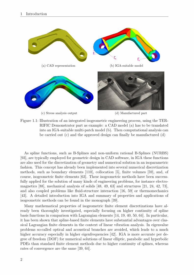
For the spatial semi-discretization of the structural vibration problem we rely on theisogeometric finite element method. In order to overcome the gap between computer-aided design, numerical simulation and manufacturing, isogeometric analysis (IGA) wasintroduced by Hughes et al. in 2005 [63]. The substantial idea behind isogeometric meth-ods is the use of the same geometry representation throughout the whole engineeringprocess. This is showcased in Figure 1.1, using the so-called “TERRIFIC Demonstrator”,a mechanical part which we use as application for the methods we develop.
1
1 Introduction
(a) CAD representation (b) IGA-suitable model
(c) Stress analysis output (d) Manufactured part
Figure 1.1: Illustration of an integrated isogeometric engineering process, using the TER-RIFIC Demonstrator part as example: a CAD model (a) has to be translatedinto an IGA-suitable multi-patch model (b). Then computational analysis canbe carried out (c) and the approved design can finally be manufactured (d)
As spline functions, such as B-Splines and non-uniform rational B-Splines (NURBS)[93], are typically employed for geometric design in CAD software, in IGA these functionsare also used for the discretization of geometry and numerical solution in an isoparametricfashion. This concept has already been implemented into several numerical discretizationmethods, such as boundary elements [110], collocation [5], finite volumes [59], and, ofcourse, isogeometric finite elements [63]. These isogeometric methods have been success-fully applied for the solution of many kinds of engineering problems, for instance electro-magnetics [88], mechanical analysis of solids [48, 49, 63] and structures [21, 24, 42, 73],and also coupled problems like fluid-structure interaction [16, 59] or thermomechanics[43]. A detailed introduction into IGA and summary of properties and applications ofisogeometric methods can be found in the monograph [39].
Many mathematical properties of isogeometric finite element discretizations have al-ready been thoroughly investigated, especially focusing on higher continuity of splinebasis functions in comparison with Lagrangian elements [14, 19, 40, 50, 64]. In particular,it has been shown that spline-based finite elements have substantial advantages over clas-sical Lagrangian finite elements in the context of linear vibration analysis. In eigenvalueproblems so-called optical and acoustical branches are avoided, which leads to a muchhigher accuracy especially in higher eigenfrequencies [42]. IGA is more accurate per de-gree of freedom (DOF) for numerical solutions of linear elliptic, parabolic and hyperbolicPDEs than standard finite element methods due to higher continuity of splines, whereasrates of convergence are the same [39, 64].
2

1.1 Scope and context
Isogeometric analysis has also been applied in nonlinear continuum mechanics and in-compressible elasticity, where the above-mentioned advantages of the approach could alsobe verified [6, 48, 84, 118]. The special treatment of incompressible and near incompress-ible problems using mixed elements [84, 118], reduced integration [24], or strain projectionmethods [48] is especially important for the simulation of rubber and elastomer materi-als. Here, we employ a mixed formulation based on [6, 7, 23, 109] for the isogeometricfinite element discretization of (near) incompressible materials and then also include itin nonlinear frequency analysis. A special focus lies on comparison of different kinds ofisogeometric mixed elements, namely Taylor-Hood and subgrid elements, which were sofar used and investigated only for the linear Stokes problem [28].
As outlined above, isogeometric finite element methods (IGA-FEM) offer many advan-tages over classical finite element discretizations, in particular a better integration intothe CAE process, higher accuracy per DOF, especially in frequency analysis, and a simpleand flexible implementation of mixed formulations. Consequently, they are our methodof choice and we use IGA-FEM in this thesis for the spatial semi-discretization of theequation of motion.
After the spatial semi-discretization of nonlinear elastodynamics equation, which yieldsa system of nonlinear ordinary differential equations (ODEs), we employ the harmonicbalance method (HBM) for time domain discretization [86, 87, 117]. In general, HBMcan be applied for frequency and steady-state vibration analysis of periodic systems ofnonlinear ODEs, and is based on Fourier transformation and solution of the ODE in thefrequency domain.
Though harmonic balance is a well-established method for nonlinear frequency analysis,for example in the context of integrated circuit simulations [31, 106], it is so far hardlyused in mechanics, only for lower dimensional structural models such as beams and plates[80, 81, 98, 99, 100]. Within commercial finite element analysis (FEA) software, non-linear frequency response analysis has to be carried out as transient analysis using timeintegration methods, either integrating until steady state is reached or using shootingmethods.
Having studied the use of isogeometric finite elements in combination with harmonicbalance for the nonlinear Euler-Bernoulli beam model already in [126, 127], we extendthe method to 3-dimensional continuum mechanics and elastodynamics [128]. As HBMuses a truncated Fourier expansion of length m for frequency domain approximation ofeach DOF of the spatial discretization, it produces a blow-up of total DOFs: the sparselinear system to be solved in the end is not only m-times larger, but also with m-timesas many nonzero entries per row than the matrix arising from spatial discretization.
Therefore model order reduction (MOR) of the spatial discretization is needed to reducethe size of the linear system significantly and make an efficient numerical solution of thesystem arising from HBM possible. In linear FEA and vibration analysis, modal reductionis a well-established technique [62]. There, the equation of motion is projected onto asubspace spanned by a subset of eigenmodes. However, for nonlinear problems moreadvanced methods are needed [94, 130]. For example, nonlinear normal modes (NNMs)[77, 119] or Proper Orthogonal Decomposition (POD) [17, 60, 112] can be used.
We propose to use a projection with eigenmodes and additionally modal derivatives[68, 111], which are a second-order enhancement of linear eigenmodes, for the use in non-linear frequency analysis [128]. In contrast to most other common reduction methods so
3

1 Introduction
far used in nonlinear dynamics, it does not require a current state of deformation of thesystem and continuous basis updates, thus the projection basis can be fully precomputedbased on the linearized system. Furthermore, there are also similar well-established tech-niques of second-order enhancements in other fields of computational engineering such asuncertainty quantification [101].
The reduction method using eigenmodes and modal derivatives has been successfullyapplied in nonlinear dynamic analysis by time integration before [11, 12, 96, 112], and weshow that it is especially suitable in our nonlinear vibration framework with harmonicbalance and makes a large-scale application of nonlinear frequency analysis possible.
1.2 Publications and software
Within the course of preparing this thesis, the author has already published intermediateresults and achievements in scientific journals and conference proceedings. Isogeometricfinite elements and harmonic balance with application to the nonlinear Euler-Bernoullibeam structural model were investigated in the diploma thesis [126] and published in[127]. The application to 3-dimensional nonlinear elasticity with large deformations andhyperelastic constitutive laws, as well as the use of reduction with modal derivatives werepublished in [128]. Implementation of isogeometric mixed Taylor-Hood elements and theirperformance in static nonlinear incompressible elasticity were investigated as part of [33].Linear elasticity computations for evaluation of an isogeometric segmentation pipeline forthe generation of analysis-suitable multi-patch models from CAD models were contributedto [89].
We have implemented the methods and tested the computational examples presented inthis thesis in different software packages. The results related to the linear and nonlinearbeam were obtained using a MATLAB implementation. All methods for 3-dimensional elas-ticity are related to the development of IGAsolvers C++-library within the TERRIFICEU-project [53]. They are partially available for download and use under GNU LesserGeneral Public License (LGPL) at [121]. Mixed methods for static nonlinear incompress-ible elasticity were also implemented in C++ using igatools library [91].
1.3 Outline
This thesis is structured in 7 chapters. After this introductory chapter we give a summaryof the main ideas behind isogeometric analysis and isogeometric finite element discretiza-tions in Chapter 2. As it is an important aspect of the simulation of complex real-lifegeometries, we set a focus on the treatment and implementation of multi-patch problems.
In Chapter 3 we review the theory of nonlinear continuum mechanics, including largedeformation kinematics and visco-hyperelastic constitutive relations, and apply the iso-geometric finite element method for the spatial discretization. We also present theoryand discretization of linear elasticity and the nonlinear Euler-Bernoulli beam, and showcomputational applications for validation of our implementations.
Then we treat nonlinear vibration analysis in Chapter 4, introduce the harmonic bal-ance method and apply it to nonlinear continuum mechanics and dynamics. We usecomputational applications to validate the approach and to examine convergence of theisogeometric discretization and truncated Fourier series.
4

1.3 Outline
Chapter 5 is dedicated to model order reduction and its application to nonlinear vibra-tion analysis. We motivate the use of a novel projection method with modal derivatives,explain it in detail, and study it analytically and numerically.
We introduce isogeometric mixed methods for near incompressible elasticity problemsin Chapter 6. We outline their integration into harmonic balance method and studytheir performance in numerical examples for static nonlinear deformation and nonlinearfrequency analysis problems.
Finally, Chapter 7 concludes this thesis with a summary and an outlook on futureresearch directions.
5

6
2 Isogeometric analysisand finite elements
This chapter provides a basic introduction into the concepts of isogeometric analysis andisogeometric finite elements, which we use for the spatial discretization of the vibrationproblem.
Spline functions have been an essential foundation of CAD over the past decades andthus we briefly review their definition and properties in Section 2.1. The idea behindisogeometric analysis is to employ splines also for the numerical solution of PDEs, forexample in a finite element method. Since much research has been done on the field ofisogeometric methods in the past years, we present only the basic ideas and propertiesrelevant in this work in Section 2.2. We lay a special focus on the treatment of multi-patchproblems, where the computational domain is decomposed into several spline geometries.In Section 2.3 we present and compare two strategies for the implementation of constraintsfor multi-patch problems.
2.1 B-Splines and NURBS
B-Splines and Non-Uniform Rational B-Splines (NURBS) are the tools that are typi-cally used for describing geometries in computer-aided design and also for representingthe numerical solution in isogeometric analysis [39, 51, 63, 93]. Detailed definitions andintroductions, including proofs and computer implementations can be found in [93], while[102] also includes an historical perspective on the topic. Here a brief review of the maindefinitions and properties is given.
2.1.1 B-Spline and NURBS basis functions
Starting point is the definition of a knot vector Ξ = (ξ1, . . . , ξm) as a non-decreasingsequence of knots ξi ∈ R (i = 1, . . . ,m) , ξi ≤ ξi+1 (i = 1, . . . ,m − 1) on the parameterspace Ω0 = [ξ1, ξm] ⊂ R.
In the following, some terminology associated with the knot vectors will be useful. IfΞ is a knot vector we use Ξ0 to refer to the corresponding distinct knot vector where allknots of Ξ0 have multiplicity one. The half-open interval [ξi, ξi+1) is called the i-th knotspan or element. The total number of nonzero knot spans or elements in Ξ is `. The
7

2 Isogeometric analysis and finite elements
length of a knot span is hi = ξi+1 − ξi (i = 1, . . . , `) and h = mini=1,...,` hi is the meshparameter. If the knots ξi are uniformly distributed over Ξ, then we call the knot vectoruniform, and if the first and last knot have multiplicity p + 1, i.e. ξ1 = . . . = ξp+1 andξm−p = . . . = ξm, the knot vector is called open.
Definition 2.1 (B-Spline basis functions). The B-Spline basis functions Bpi (ξ) : Ω0 →
[0, 1] of degree p (order p+ 1) are defined for i = 1, . . . , n (n = m− p− 1) by the Cox-deBoor recursion:
B0i (ξ) =
1 ξi ≤ ξ < ξi+1
0 else,
Bpi (ξ) = ξ − ξi
ξi+p − ξiBp−1i (ξ) + ξi+p+1 − ξ
ξi+p+1 − ξi+1Bp−1i+1 (ξ).
(2.1)
Here it is assumed that the quotient 0/0 is 0.
There are many useful properties of B-Spline basis functions Bpi , i = 1, . . . , n, and
among them we point out that they• are piecewise polynomials of degree p,• have compact support, i.e. supp(Bp
i ) = [ξi, ξi+p+1),• are non-negative, i.e. Bp
i (ξ) ≥ 0 ∀ξ ∈ [ξ1, ξm],• form a partition of unity for an open knot vector, i.e. ∑n
i=1Bpi (ξ) ≡ 1 ∀ξ ∈ [ξ1, ξm],
• are smooth, i.e. they are p-times continuously differentiable (Cp-continuous) insidea knot span and at inner knots of multiplicity k (k ≤ p) only Cp−k.
Here we only use B-Spline basis functions on open knot vectors with inner knots ofmultiplicity 1 ≤ k ≤ p.
Example 2.1 (Different types of B-Spline basis functions on the same distinct knotvector). An example of B-Spline basis functions with different degrees and continuitiesbased on the same distinct knot vector Ξ0 = (0, 0.2, 0.4, 0.6, 0.8, 1) can be found in Figure2.1:
(a) Ξ = (0, 0, 0.2, 0.4, 0.6, 0.8, 1, 1), p = 1, m = 8, n = 6:linear with C0-continuity at all inner knots
(b) Ξ = (0, 0, 0.2, 0.4, 0.6, 0.8, 1, 1), p = 2, m = 10, n = 7:quadratic with C1-continuity at all inner knots
(c) Ξ = (0, 0, 0, 0.2, 0.4, 0.6, 0.8, 1, 1, 1), p = 3, m = 12, n = 8:cubic with C2-continuity at all inner knots
(d) Ξ = (0, 0, 0, 0.2, 0.4, 0.4, 0.6, 0.8, 0.8, 1, 1, 1), p = 3, m = 15, n = 11:cubic with C1-continuity at ξ = 0.4, C0-continuity at ξ = 0.8 and C2-continuity atall other knots
Definition 2.2 (Non-Uniform Rational B-Spline basis functions). The definition of Non-Uniform Rational B-Spline (NURBS) basis functions Np
i is based on B-Spline basis func-tions Bp
i on a knot vector Ξ and additional weights wi > 0 (i = 1, . . . , n):
Npi (ξ) = Bp
i (ξ) wi∑nj=1B
pj (ξ) wj
. (2.2)
8

2.1 B-Splines and NURBS
0 0.2 0.4 0.6 0.8 10
0.2
0.4
0.6
0.8
1
ξ
Ni1 (ξ
)
(a) Linear C0 B-Spline basis functions
0 0.2 0.4 0.6 0.8 10
0.2
0.4
0.6
0.8
1
ξ
Ni2 (ξ
)
(b) Quadratic C1 B-Spline basis functions
0 0.2 0.4 0.6 0.8 10
0.2
0.4
0.6
0.8
1
ξ
Ni3 (ξ
)
(c) Cubic C2 B-Spline basis functions
0 0.2 0.4 0.6 0.8 10
0.2
0.4
0.6
0.8
1
ξ
Ni3 (ξ
)
(d) Cubic B-Splines with mixed continuities
Figure 2.1: Different types of B-Spline basis functions on the same distinct knot vector
Efficient algorithms for the evaluation of B-Spline and NURBS basis functions and theirderivatives are described in detail in [93].
NURBS are piecewise rational functions and the essential properties of B-Splines givenabove hold for NURBS as well. For equal weights, i.e. wi = const. ∀i = 1, . . . , n, NURBSreduce to B-Spline basis functions and thus in the following we are only using the termNURBS.
Definition 2.3 (Spline spaces). The vector space of NURBS basis functions of degree pand minimum continuity k ≤ p− 1 on the open knot vector Ξ is denoted by
Skp (Ξ) = spanNpi i=1,...,n. (2.3)
Note that dim(Skp (Ξ)) = m− p− 1 = n and Npi actually are a basis of Skp (Ξ), since they
are linearly independent.
2.1.2 Spline geometries
In CAD programs geometry is typically represented by spline curves and surfaces. Theadditional benefit of NURBS over B-Splines is the possibility to represent conic inter-sections exactly, which is very important for designing engineering shapes. Here we in-troduce spline curves and volumes, since we need to have a solid representation for our3-dimensional applications.
9

2 Isogeometric analysis and finite elements
0 0.25 0.5 0.75 10
0.25
0.5
0.75
1
ξ
Ri2 (ξ
)
(a) Quadratic NURBS basis functions of the circle−1 −0.5 0 0.5 1
−1
−0.5
0
0.5
1
(b) Circle (blue) with control points (red) and con-trol polygon (dashed red)
Figure 2.2: A circle as a NURBS curve
Definition 2.4 (Spline curve). A spline curve c : Ω0 → Rd is defined by a spline spaceSkp (Ξ) and control points ci ∈ Rd (i = 1, . . . , n):
c(ξ) =∑i=1
Npi (ξ) ci. (2.4)
Spline curves as defined above have the following properties:• The polygon formed by the control points cii=1,...,n is called control polygon.• Convex hull property, i.e. the curve is completely contained in its control polygon.• Interpolation of start and end points, i.e. c(ξ1) = c1 , c(ξm) = cn.• Affine invariance, i.e. affine transformations of the curve can be performed on its
control points.• Displacing a control point ci only influences the curve locally in the knot interval
[ξi, ξi+p+1).• The continuity properties of the curve correspond to the ones of B-Spline/NURBS
functions.
Example 2.2 (A circle as a NURBS curve). A typical example used to illustrate thecapabilities of NURBS is the exact representation of a circle. In Figure 2.2 a circleof radius 1 around the origin is shown. The knot vector of the quadratic NURBS basisfunctions is Ξ = (0, 0, 0, 1
4 ,14 ,
12 ,
12 ,
34 ,
34 , 1, 1, 1), i.e. p = 2, m = 12, n = 9, weights are w =
(1, 12
√2, 1, 1
2
√2, 1, 1
2
√2, 1, 1
2
√2, 1) and control points of the curve are ( 1
0 ), ( 11 ), ( 0
1 ), ( −11 ),
( −10 ),
(−1−1
), ( 0−1 ), ( 1
−1 ), ( 10 ).
10

2.1 B-Splines and NURBS
Figure 2.3: A train wheel as a NURBS volume. Showing the control points (blue), thecontrol point mesh (red) and the volume itself (gray)
It is possible to define multivariate NURBS functions, for example in 3D, as productof univariate NURBS:
Np1p2p3i1i2i3 (ξ1, ξ2, ξ3) = wi1wi2wi3B
p1i1 (ξ1)Bp2
i2 (ξ2)Bp3i3 (ξ3)∑n1
j1=1∑n2j2=1
∑n3j3=1wj1wj2wj3B
p1j1 (ξ1)Bp2
j2 (ξ2)Bp3j3 (ξ3) , (2.5)
where Np1p2p3i1i2i3 : Ω1
0 × Ω20 × Ω3
0 → R.Since this notation is very laborious and we are going to deal with trivariate NURBS
many more times in this work, in the following n, p, i should be understood as 3-dimension-al multi-indices n = (n1, n2, n3), p = (p1, p2, p3) and i = (i1, i2, i3), giving the number,degree and index of trivariate NURBS functions Np
i (ξ) with parameters ξ = (ξ1, ξ2, ξ3).The reference domain Ω0 = Ω1
0 × Ω20 × Ω3
0 and mesh or triangulation Ξ = Ξ1 × Ξ2 × Ξ3
are defined using the Cartesian product of domains resp. knot vectors of each parameterdirection.
Definition 2.5 (Spline volume). A spline volume v : Ω0 → R3 is defined by a trivariatespline space Skp (Ξ) and a mesh of control points vi ∈ R3:
v(ξ) =n∑i=1
Npi (ξ) vi. (2.6)
Example 2.3 (A train wheel as a NURBS volume). Figure 2.3 shows a simplified modelof a train wheel as a NURBS volume. The volume itself is displayed in gray, the controlpoints in blue and the control mesh in red. The NURBS basis functions are quadratic inall three directions and the volume has 504 basis functions and control points in total.
11

2 Isogeometric analysis and finite elements
0 0.5 10
1
ξ
Ni1 (ξ
)
Initial B-spline basis functions, Ξ = (0, 0, 1, 1)
0 0.5 10
1
ξ
Ni1 (ξ
)
↓
0 0.5 10
1
ξ
Ni2 (ξ
)
↓
0 0.5 10
1
ξ
Ni3 (ξ
)
(a) p-method: knot insertion, then twice order ele-vation, Ξ∗
a = (0, 0, 0, 0, 0.5, 0.5, 0.5, 1, 1, 1, 1)
0 0.5 10
1
ξ
Ni2 (ξ
)↓
0 0.5 10
1
ξ
Ni3 (ξ
)
↓
0 0.5 10
1
ξ
Ni3 (ξ
)
(b) k-method: two order elevations, then knot in-sertion, Ξ∗
b = (0, 0, 0, 0, 0.5, 1, 1, 1, 1)
Figure 2.4: Comparison of refinement strategies: p-method and k-method
2.1.3 Refinement
An important feature of B-Spline and NURBS geometries is the possibility to refine aspline geometry without changing its shape. There exist three basic types of refinement,which are described in the following when applied to a univariate spline space (Def. 2.3)resp. a spline curve (Def. 2.4). For more details see [39].
h-refinement
h-refinement or knot insertion means that a given knot vector Ξ is extended to Ξ∗ byintroducing an additional knot ξ∗ ∈ Ω0 such that Ξ ⊂ Ξ∗. This provides a new set ofn+1 basis functions and a new set of n+1 control points c∗i has to be computed as linear
12

2.1 B-Splines and NURBS
combinations of the original control points ci.A knot insertion step can be used to split an element into two by adding a new distinct
knot, similar to the h-refinement process in classical finite element analysis. But here thecontinuity at the new knot is Cp−1, while it is C0 in FEA. It is also possible to decreasecontinuity of basis functions at an existing knot by increasing its multiplicity.
In this work usually h-refinement refers to a uniform refinement of the knot vector.This means that in every nonempty knot interval [ξi, ξi+1) a new knot ξ∗i = (ξi+1 + ξi)/2is inserted. Thus the number of knots increases to m∗ = m + `, the number of elementsto `∗ = 2` and n∗ = n+ `. The mesh parameter of the refined knot vector Ξ∗ is h∗ = h/2.
p-refinement
p-refinement or order/degree elevation is used to increase the polynomial degree of thespline space to p∗ = p + 1. The multiplicity of all distinct knots has to be increased byone for the new knot vector Ξ∗, in order to maintain Cp−1 continuity at inner knots, i.e.Skp (Ξ0) is refined to Skp+1(Ξ0).
This strategy is similar to p-refinement in FEA resp. p-FEM, where higher degreepolynomials are used on element level. However, in IGA continuity at inner knots ismaintained and not reduced to C0.
After p-refinement it is m∗ = m+ `+ 1, `∗ = `, n∗ = n+ ` and h∗ = h.
k-refinement
When a series of h- and p-refinements is performed, its order influences the result, i.e. therefinement strategies do not commute. k-refinement means that p-refinements are carriedout before any h-refinement steps, since this leads to a minimal multiplicity resp. maximalcontinuity of inner knots. The differences between refinement strategies are illustratedwith the following example.Example 2.4 (Comparison of refinement strategies). As simple example for the compar-ison of different refinement strategies is presented in Figure 2.4. We start from the knotvector Ξ = (0, 0, 1, 1), Ξ0 = (0, 1), defining the linear B-Spline space S0
1 (Ξ0). We want toadd the knot ξ∗ = 0.5 and degree-elevate twice to p∗ = 3:
(a) p-method: first h-refinement and then two p-refinements lead to Ξ∗a = (0, 0, 0, 0, 0.5,0.5, 0.5, 1, 1, 1, 1). The final spline space has p∗a = 3, m∗a = 11, n∗a = 7 with C0-continuity at ξ = 0.5.
(b) k-method: first two p-refinements and then h-refinement, i.e. k-refinement, lead toΞ∗b = (0, 0, 0, 0, 0.5, 1, 1, 1, 1). The final spline space has p∗b = 3, m∗b = 9, n∗b = 5with C2-continuity at ξ = 0.5.
Remark 2.1. In numerical studies for the comparison of performance of isogeometric vs.classical finite elements, the k-method is typically, and also in this thesis, associated withIGA and the p-method with FEM [42].
Local refinement
Due to the tensor product structure of spline meshes, the above presented p/h/k-refine-ment strategies have a global impact on the meshes. Degree elevation can of course only
13

2 Isogeometric analysis and finite elements
(a) Original mesh (b) after one h-ref. (c) after two h-ref.
Figure 2.5: Tensor product refinement with knot insertion
(a) Original mesh (b) after one local ref. (c) after two local ref.
Figure 2.6: True local refinement
be applied to a complete knot vector and also knot insertion in the knot vector of oneparameter dimension has a global effect on the tensor product mesh, see Example 2.5.
For a true local refinement of spline meshes the tensor product structure must becircumvented or avoided. Several attempts have been developed, such as hierarchicalB-Splines (HB-Splines) [52], splines on T-meshes (T-Splines) [107] and locally refined B-Splines (LR B-Splines) [44]. They have all been successfully applied also in the contextof isogeometric analysis and isogeometric finite element methods [15, 69, 125], but arebeyond the scope of this thesis.
Example 2.5 (Visualization of global vs. local refinement strategies). The effect of globalrefinement is visualized in Figure 2.5, where one would like to refine around the bottomleft corner of the initial 2-dimensional mesh (a). In both knot insertion steps (b) and (c)one knot in inserted in each knot vector, but this carries on in the tensor product mesh tothe top left and bottom right corners.
Instead, one would like to do a true local refinement of only the bottom left area, as itis shown in Figure 2.6 and as it is possible for classical finite element meshes or advancedrefinement methods such as hierarchical splines or T-splines.
2.2 Isogeometric finite element method
As discussed in the introductory chapter, the main idea behind isogeometric analysis(IGA) is to bridge the gap between CAD and FEM. Based on [39, 63] we summarize nowthe major properties and discuss the relation to classical finite elements.
14

2.2 Isogeometric finite element method
The key ingredients of IGA are spline basis functions and geometries, as introduced inthe previous Section 2.1, which are used for both representing the geometry and spanningthe solution spaces in the Galerkin method. The isoparametric concept of classical FEMemploys also the same function spaces for representation of geometry and solution, butthere a conversion step is applied, where the CAD geometry is approximated by thesepiecewise polynomials. On the other hand, IGA with NURBS makes it possible to bypassthis conversion and mesh generation step, and moreover offers higher continuity of thenumerical approximation.
2.2.1 Isogeometric Galerkin discretization
We introduce the concept of an isogeometric finite element discretization of a linear partialdifferential equation in a general setting:
Definition 2.6 (Variational formulation of PDE problem). We seek a solution u ∈ S ofthe variational or weak formulation of a partial differential equation on a domain Ω ⊂ Rd
using test functions v ∈ V, where S = u : u ∈ (H1(Ω))r,u|δΩ = h, V = v : v ∈(H1(Ω))r, v|δΩ = 0, a(·, ·) is a bilinear form, l(v) = 〈v, f〉 a linear form, f the right handside function, 〈·, ·〉 the standard L2-scalar product, and r the range of the solution space:
u ∈ S : a(v,u) = l(v) ∀ v ∈ V . (2.7)
Existence and uniqueness of the solution are guaranteed by the theorem of Lax-Milgramif a(·, ·) is continuous and coercive and l(·) is coercive.
The idea behind isogeometric analysis is that the domain Ω of problem (2.7) is givenin terms of a geometry function g, which maps a reference domain Ω0 ⊂ Rd0 , 1 ≤ d0 ≤ d,onto the physical domain of the problem:
g : Ω0 → Ω, x = g(ξ). (2.8)
This geometry function or parameterization can be expressed in terms of a spline geometry,here a NURBS volume, see (2.6):
x = g(ξ) =n∑i=1
Npi (ξ)vi. (2.9)
Then Galerkin’s method is applied, i.e., the infinite-dimensional function spaces S andV are approximated by finite-dimensional subspaces Sh ⊂ S and Vh ⊂ V . Following theisoparametric paradigm, these spaces are spanned by the push-forward of the NURBSbasis functions of the geometry function g onto the physical domain Ω (or a refinementthereof):
Sh ⊂ spanNpi g−1
r, uh(x) =
n∑i=1
Npi
(g−1(x)
)di
Vh ⊂ spanNpi g−1
r, vh(x) =
n∑i=1
Npi
(g−1(x)
)δdi,
(2.10)
where di, δdi ∈ Rr are the control points of displacements and virtual displacements.
15

2 Isogeometric analysis and finite elements
Substituting uh and vh from (2.10) into the weak form (2.7) and making use of thebilinearity of a(·, ·) and linearity of l(·) yields
δdT K d = δdT b ∀δd ∈ RN , (2.11)
with N = rn, stiffness matrix K ∈ RN×N and load vector b ∈ RN ,
Kklij = a(Np
i 1k, Npj 1l) , i = 1, . . . , n, j = 1, . . . , n, k = 1, . . . , r, l = 1, . . . , r
bki = l(Npi 1k) , i = 1, . . . , n, k = 1, . . . , r,
(2.12)
where 1k is the r-dimensional unit vector with a 1 in direction k.The displacement vector d = (dT1 , . . . ,dTn )T is then computed by solving a linear system
K d = b, (2.13)
which results in the approximate displacement uh in the form of a spline geometry.For the evaluation of (2.12) integrals over the physical domain Ω in a(·, ·) and l(·)
are transformed and computed on the parameter domain Ω0 using ξ = g−1(x). In thesame fashion, derivatives of uh(x) with respect to x can be transformed to derivativeswith respect to ξ using the chain rule. Thus it is necessary to compute the Jacobianof the geometry function Dg(ξ) = (∂gi/∂ξj)ij and its inverse, which requires that theparameterization is invertible and the inverse is also continuous.
The entries of K and b are computed by quadrature rules at the element level and thenassembled into the global stiffness matrix and load vector. A Gaussian quadrature rule isused with p+ 1 quadrature points on each knot span, very similar to classical FEM, withknot spans playing the role of elements, see [62, 66] for more details.
2.2.2 Properties of isogeometric finite elements
As the isogeometric finite element discretization is a Galerkin method, just as the classicalfinite element method, many mathematical properties of FE discretizations can be car-ried over to isogeometric finite elements [14, 64, 114]. A summary of numerical analysisproperties of isogeometric finite element methods can be found in [19].
In the following we use some abbreviations for standard norms
‖ · ‖ := ‖ · ‖L2(Ω)r , ‖ · ‖p := ‖ · ‖Hp(Ω)r , ‖ · ‖E :=√a(·, ·) (2.14)
and σ = min p + 1, 2(p + 1 − m), where 2m is the order of the differential operatorfrom which a(·, ·) is derived.
A-priori error estimates
For linear elliptic boundary value problems such as (2.7) with sufficiently regular exactsolution and data, standard error estimates from FEM are also valid for isogeometric FE[64, 114]:
‖u− uh‖E ≤ Chp+1−m ‖u‖p+1,
‖u− uh‖ ≤ Chσ ‖u‖p+1.(2.15)
16

2.2 Isogeometric finite element method
The major difference between classical finite elements and IGA is the continuity of basisfunctions: while a FE discretizations consists of many small elements with polynomialsas element-wise basis functions and C0-continuity over element boundaries, isogeometricspline discretizations have a higher continuity of maximum Cp−1 over knots, i.e. elementboundaries. But this advantage of IGA, which usually becomes obvious in numericalresults, is not reflected in the standard error estimates (2.15).
However, in [50] it was shown that higher degree spline spaces with maximal continuityare optimal for the approximation of many function spaces such as L2- and H1-spaces.In numerical studies the k-method provided much better results than the p-method, thussuggesting that IGA can be more accurate than FEM per DOF.
Eigenvalue problems
In [41, 42, 65] the properties of IGA in wave propagation and eigenvalue problems, i.e.modal or linear vibration analysis, were investigated and compared to standard FEM. Inthe same fashion of (2.7), we can write the eigenvalue problem as follows:
ui ∈ S, ωi ∈ R : ω2i 〈v,ui〉+ a(v,ui) = 0 ∀ v ∈ V . (2.16)
The discrete spectra of numerical approximations vs. analytical eigenfrequencies ωhi /ωiwere analyzed for one-, two- and three-dimensional cases. As shown with the example inFigure 2.7, higher continuity of splines is very beneficial for the accuracy of eigenfrequencyapproximations. While the p-method leads to optical and acoustical branches in thespectra for higher degrees of p ≥ 3 and a very low accuracy with divergent behavior fori→ n, the spectra for the isogeometric k-method are smooth with a much higher accuracyover the whole domain. Only at the end of the spectrum a few outliers occur, which arediscussed in detail in [42]. In the 1D cases of linear string and beam vibrations, wherea(u, v) =
∫Ω v′ u′dx resp. a(u, v) = −
∫Ω v′′ u′′dx, it is even possible to compute the spectra
analytically and verify the numerical results [42].In [64, 114] the following relations and error bounds for FEM and IGA approximation for
eigenfunctions ui and eigenvalues λi = ω2i were established, when the smallness condition
hλ1/(2m)i ≤ ε is fulfilled:
‖uhi − ui‖2 + λhi − λiλi
= ‖uhi − ui‖2
E
λi,
λhi − λiλi
≤ C(hλ
1/(2m)i
)2(p+1−m),
‖uhi − ui‖Eλ
1/2i
≤ C(hλ
1/(2m)i
)p+1−m,
‖uhi − ui‖ ≤ C(hλ
1/(2m)i
)σ.
(2.17)
Due to the smallness condition, these approximation estimates only hold for the lowerpart of the spectrum up to some wave number i n. Nevertheless, in [64] it could beshown numerically that the whole spectrum of eigenfunctions can be approximated muchmore accurately with smooth splines than with C0 finite elements.
17

2 Isogeometric analysis and finite elements
0 0.1 0.2 0.3 0.4 0.5 0.6 0.7 0.8 0.9 11
1.1
1.2
1.3
1.4
1.5
1.6
1.7
1.8
1.9
2
i / n
ωh i /
ωi
p=2
p=3 (IGA)
p=4 (IGA)
p=5 (IGA)
p=6 (IGA)
p=7 (IGA)
p=3 (FEM)
p=4 (FEM)
p=5 (FEM)
p=6 (FEM)
p=7 (FEM)
p
p
FEM
IGA
Figure 2.7: Comparison of discrete spectra of eigenfrequencies ωhi /ωi for a linear beam forC1-continuous p-method (FEM) and Cp−1-continuous k-method (IGA)
Time-dependent problems
The impact of approximation accuracy of eigenvalues and eigenfunctions on time-depen-dent problems, such as parabolic and hyperbolic linear PDEs, was also investigated in[64]. In the error estimates of parabolic problems, the influence of poorly approximatedhigher modes is damped out by an exponentially decaying factor eλit . In contrast to that,for hyperblic problems, as they are treated in this thesis, the errors in higher modes andin the modal projection of the initial data persist for all time. Thus significant errors ineigenfunctions, as they occur for standard FEM already in the mid and higher spectrum,can also significantly contribute to the error of the time-dependent solution, especially innonlinear applications. In these situations much more accurate results can be expectedfrom IGA, since approximation quality of higher modes is much better.
Computational costs
An important argument for the use of IGA or FEM in practical applications are thecomputational costs, which mainly consist of the assembly of the stiffness matrix (2.12)and solution of the linear system (2.13). [19, 105] feature comparisons of the influence ofcontinuity of basis functions, C0 (FEM) or Cp−1 (IGA), on computational costs:
Assuming periodicity boundary conditions of maximal continuity and r = d, the numberof DOFs is N = pd` for C0 and N = ` for Cp−1 basis functions. In both cases the local,element-wise contributions to the stiffness matrix have to be computed using numericalquadrature with a cost of O(p2d) operations per quadrature point, independent of thecontinuity. Using Gaussian quadrature with (p + 1)d points per element, we have `(p +1)d points in total. In terms of N , this means O(Np3d) operations in the C0 case andO(Np3(d+1)) in the Cp−1 case. Thus assembly is more costly for the same number of DOFsin IGA than in FEM. To alleviate this disadvantage of IGA and reduce the quadrature
18

2.3 Multi-patch parameterizations
effort, advanced quadrature [8, 66] and assembly strategies have been developed [71, 82].Higher continuity also influences the number of nonzeros of the stiffness matrix and its
sparsity pattern. In the C0 case the total number of nonzeros is nnz = (p + 2)dpd` =(p + 2)dN , while it is nnz = (2p + 1)d` = (2p + 1)dN for Cp−1 basis functions [19]. Sofor same N there are more nonzeros in the IGA stiffness matrix, i.e. it is more densely-populated than a FEM matrix. This has a severe impact on the performance of linearalgebra solvers used to solve the system (2.13). Direct solvers consume more memory forIGA then for FEM and solution times are longer. The performance of iterative solversmainly depends on the number of iterations, the cost of one iteration, and preconditioningand was investigated in [36]. Preconditioning techniques have been adapted to IGA tomake iterative solution of large systems more efficient, where a summary of methods,including Overlapping Schwarz, BPX, BDDC, multigrid, and FETI, is presented in [19].
In a competitive isogeometric finite element analysis software library, which could keepup with established and commercial finite element analysis codes and software regardingcomputational times, the above-mentioned quadrature strategies and solution techniquesshould be implemented. However, due to limited time and resources, they could not beconsidered in the IGAsolvers software developed within the course of this thesis [121].
2.3 Multi-patch parameterizations
So far we have assumed that the physical domain Ω can be represented by a geometryfunction in terms of a single spline geometry, see (2.8) and (2.9). However, complexengineering designs available as CAD models can usually not be represented as a single,tensor product spline geometry, since the topology of the object differs from a rectangle in2D or a cube in 3D [40]. Then an isogeometric analysis suitable parameterization has tobe generated by splitting the object into several parts (patches), with geometry functionsmapping reference domains onto the physical domains for each patch. In the following wedescribe the treatment of multi-patch domains in isogeometric finite element analysis.
2.3.1 Formulation of multi-patch problems
In a multi-patch problem we have a partition of the initial domain Ω into b subdomains(patches):
Ω =b⋃i=1
Ωi, Ωi ∩ Ωj = ∅. (2.18)
If two patches Ωi and Ωj are adjacent, i.e.
Ωi ∩ Ωj = Γij 6= ∅, (2.19)
we call Γij the interface between Ωi and Ωj.To find the solution u ∈ S of the general PDE problem, see (2.7), we have to solve
it on each patch for ui = u|Ωi and need to add constraints for the displacements to becontinuous on the interfaces of the patches:
i = 1, . . . , b : ui ∈ S i = S|Ωi :a(vi,ui) = l(vi) ∀ vi ∈ V i = V|Ωi ,
ui = uj on Γij. (2.20)
19

2 Isogeometric analysis and finite elements
Parameterization of the geometry of the object is now given by a set of geometry functionsgi : Ωi
0 → Ωi as spline geometries for each patch, compare (2.8) and (2.9).Even though IGA claims to bridge the gap between design and analysis, multi-patch
parameterizations of real-life objects as spline volumes are not trivially found. Typi-cally in CAD only the boundary surfaces of an object are represented and multi-patchspline volume parameterizations have to be generated based on these surface descriptions.These parameterizations may only approximate the original CAD geometries and do notnecessarily represent them exactly. Automated methods for segmentation into patchesand parameterization of patches are still under development [70, 74, 89]. In fact, for asmooth and lossless isogeometric design through analysis process, the incorporation ofspline functions into numerical methods is not enough, it also requires a change in theproduct design approach [45].
An example can be found in Figure 3.8 in Section 3.5.2, which shows the geometryof the “TERRIFIC Demonstrator” as CAD model and an analysis-suitable multi-patchparameterization consisting of 15 volume patches.
2.3.2 Enforcement of continuity constraints
For the solution of the multi-patch PDE problem (2.20), discrete isogeometric finite el-ement solution spaces Shi ⊂ S i and test function space Vhi ⊂ V i have to be generatedbased on the patch-wise geometry functions gi, as in (2.10). Then stiffness matrices Ki
and force vectors bi can be assembled for each patch as in (2.12).Furthermore, the continuity constraints ui = uj on Γij have to be discretized and
enforced. Thereby in general two cases can be distinguished: conforming and non-conforming parameterizations.
Conforming parameterizations
A multi-patch model has conforming parameterizations, when
gi|Γij ≡ gj|Γij ∀ Γij. (2.21)
In a 3D model this means that the two spline surfaces gi|Γij and gj|Γij of the neighboringpatches i and j of the interface Γij must be identical, i.e. degrees, knot vectors, weightsand control points of the geometry functions coincide. Then the continuity constraint forthe discretized solutions uhi and uhj is simply that corresponding displacement controlpoints dik and djl have to be equal whenever the associated geometry control points vikand vjl are equal, i.e.
dik = djl ∀ dik, djl with vik = vjl . (2.22)
For the enforcement of these constraints basically two implementation strategies exist:
(a) Elimination: If dik and djl are two corresponding displacement control points inpatches i and j, the l-th row and column from Kj are removed and added to the k-throw and column of Ki, same for the right hand side vectors bi and bj. Assembly of
20
2.3 Multi-patch parameterizations
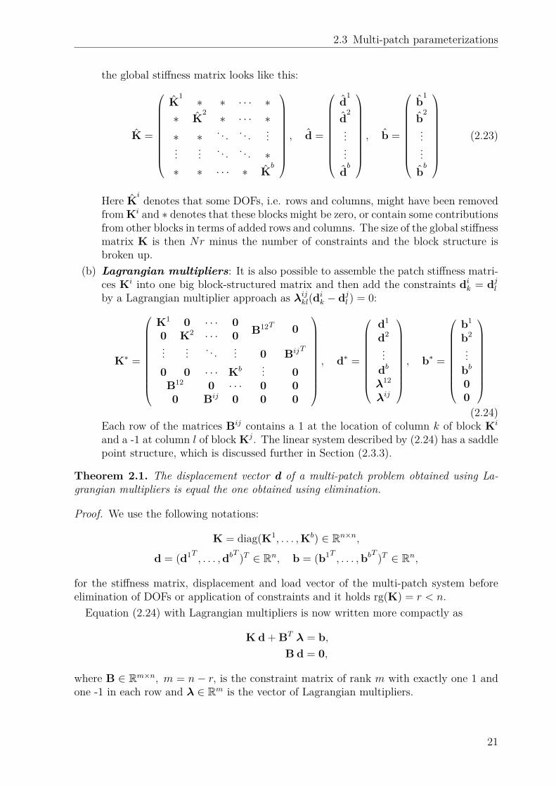
the global stiffness matrix looks like this:
K =
K1 ∗ ∗ · · · ∗∗ K
2 ∗ · · · ∗∗ ∗ . . . . . . ...... ... . . . . . . ∗∗ ∗ · · · ∗ K
b
, d =
d1
d2
...
...db
, b =
b1
b2
...
...bb
(2.23)
Here Ki denotes that some DOFs, i.e. rows and columns, might have been removed
from Ki and ∗ denotes that these blocks might be zero, or contain some contributionsfrom other blocks in terms of added rows and columns. The size of the global stiffnessmatrix K is then Nr minus the number of constraints and the block structure isbroken up.
(b) Lagrangian multipliers: It is also possible to assemble the patch stiffness matri-ces Ki into one big block-structured matrix and then add the constraints dik = djlby a Lagrangian multiplier approach as λijkl(dik − djl ) = 0:
K∗ =
K1 0 · · · 0B12T 00 K2 · · · 0
... ... . . . ... 0 BijT
0 0 · · · Kb ... 0B12 0 · · · 0 00 Bij 0 0 0
, d∗ =
d1
d2
...dbλ12
λij
, b∗ =
b1
b2
...bb00
(2.24)
Each row of the matrices Bij contains a 1 at the location of column k of block Ki
and a -1 at column l of block Kj. The linear system described by (2.24) has a saddlepoint structure, which is discussed further in Section (2.3.3).
Theorem 2.1. The displacement vector d of a multi-patch problem obtained using La-grangian multipliers is equal the one obtained using elimination.
Proof. We use the following notations:
K = diag(K1, . . . ,Kb) ∈ Rn×n,
d = (d1T , . . . ,dbT )T ∈ Rn, b = (b1T , . . . ,bbT )T ∈ Rn,
for the stiffness matrix, displacement and load vector of the multi-patch system beforeelimination of DOFs or application of constraints and it holds rg(K) = r < n.
Equation (2.24) with Lagrangian multipliers is now written more compactly as
K d + BT λ = b,B d = 0,
where B ∈ Rm×n, m = n− r, is the constraint matrix of rank m with exactly one 1 andone -1 in each row and λ ∈ Rm is the vector of Lagrangian multipliers.
21

2 Isogeometric analysis and finite elements
Assuming that there exists a projection matrix C ∈ Rn×r of rank r and a vector ofreduced DOFs d ∈ Rr such that
d = C d,
it follows:KC d + BT λ = b,
BC d = 0.
Left-multiplication of the first equation with CT , which is a rank-conserving transforma-tion on Rr, yields
CTKC d + CTBT λ = CTb,BC d = 0.
If we showed that BC = O, where O ∈ Rm×r is the m × r null matrix, it would onlyremain the equation
CTKC d = CTb,
and using K = CTKC and b = CTb, it would be the same system as in (2.23), i.e.
K d = b.
A matrix C which yields BC = O can easily be found: it is a boolean matrix withexactly one 1 in each row and at least one 1 in each column, where the total number of 1sis n. This matrix is exactly the one which assigns each of the displacement control pointsin d to one of the DOFs in d after elimination and adds the stiffness matrix contributionsof an eliminated DOF from K to the row and column of the matrix after eliminationK.
Remark 2.2. Implementation strategies for conforming parameterizations can also beextended to situations where one geometry function is an h-refinement of the other, asdescribed in [40]. This allows a simple kind of “local” refinement using multiple patches.
Remark 2.3. The Lagrangian multiplier strategy can also be used to implement generalDirichlet-type boundary conditions such as• prescription of displacements: u|ΓD = h,• symmetry of displacements w.r.t. normal direction: (u · n)|ΓD = 0,• periodicity of displacements at faces of one parameter direction: u|Γξi=0
= u|Γξi=1,
where the boundary ΓD ⊂ Γ can be a face of the topological cube (or a iso-subface), anisoline on a face (or a subline) or a point on a face. Γξi=0 and Γξi=1 refer to the faces ofthe topological cube, where the parameter direction i is fixed at the minimal resp. maximalvalue.
Non-conforming parameterizations
This is the most general case, as parameterizations of the patches can be chosen arbitrarily,i.e. degrees, knot vectors and number of control points may be different. Continuity con-straints have to be enforced weakly by methods such as Nitsche’s method [3, 104], penaltymethods, mortar or Lagrangian multiplier methods [29, 61] and augmented Lagrangianmultiplier methods. These methods mostly have its origins in domain decomposition
22

2.3 Multi-patch parameterizations
x0
x1x2
1
ξ10
ξ11
ξ12
2
ξ20
ξ21
ξ22
3
ξ30
ξ31
ξ32
4
ξ40
ξ41
ξ42
(a) Geometry with the common edge in green. Constraints on twocontrol points of each patch have to be enforced
1 2
34
(b) Constraints in red are not en-forced to avoid redundancies
Figure 2.8: Four cubes joining in one edge
of classical FEM and a summary of application in isogeometric multi-patch analysis isprovided in [3].
Due to the design of libraries used for the implementation of software developed inthe course of this thesis, the methods and applications presented here are restricted toconforming parameterizations. Both presented approaches for treatment of continuityconstraints, Lagrangian multipliers and elimination, have been implemented [121].
2.3.3 Saddle point problems
As described above by (2.24), the Lagrangian multiplier approach for implementationof multi-patch coupling constraints and Dirichlet-type boundary conditions leads to thesolution of a saddle point problem, i.e. a linear equation system of the form
K∗ d∗ = b∗ ⇔(
K BT
B 0
)(dλ
)=(
bc
), (2.25)
where K ∈ Rn×n, B ∈ Rm×n, n > m. The entries of c are zero and may contain nonzerosonly when inhomogeneous Dirichlet conditions are included, see Remark 2.3.
Saddle point problems arise in many engineering and scientific applications, especiallyalso in mixed formulations [20, 23], which we address in the isogeometric context lateron in Chapter 6. Thus we want to take a closer look at their properties and numericalsolution methods, where [22] serves as a main reference.
Solvability conditions
In our case the matrix K arising from (2.24) is symmetric and positive semi-definite. IfDirichlet boundary conditions had been incorporated into the patch-wise matrices, whichis usually not the case for all patches, it would be symmetric positive definite. For K tobe non-singular and (2.25) to have a unique solution a necessary and sufficient conditionis that B has full rank and ker(K) ∩ ker(B) = 0 [22].
The full rank condition rg(B) = m is not trivially fulfilled for the multi-patch couplingmatrix arising from (2.24). This can be demonstrated by a simple example of four cubesjoining in one edge, see Figure 2.8(a), or even simpler in 2D by four squares joining inone vertex. The constraint matrix for the common edge highlighted in green resp. one of
23

2 Isogeometric analysis and finite elements
the common control points would look like this:
B =
· · · 1 · · · −1 · · · 0 · · · 0 · · ·· · · 0 · · · 1 · · · −1 · · · 0 · · ·· · · 0 · · · 0 · · · 1 · · · −1 · · ·· · · −1 · · · 0 · · · 0 · · · 1 · · ·
. (2.26)
By summing up all rows it can be easily seen that this matrix is singular and that rg(B) =3. This means that one of the constraints is redundant and not to be enforced, as shownin Figure 2.8(b).
To avoid such redundancies and set up the global constraint matrix, an approach fromgraph theory can be used: every control point located on an interface is a vertex and everyconstraint is an edge of a directed graph. Then the constraint matrix B can be interpretedas incidence matrix of that directed graph with vertices in columns and edges in rows.Finding a full rank sub-matrix of B is then equivalent to finding a forest or spanningtree of the (undirected) graph, which can be done by a breadth-first or depth-first searchalgorithm [129]. In other words, we only include the constraints resp. rows in B whichcorrespond to the edges contained in the forest of the graph.
We do not explicitly check if the condition ker(K) ∩ ker(B) = 0 is fulfilled, but weexpect it due to the following considerations. In a 3-dimensional elasticity problem, oneneeds to restrict 6 degrees of freedom (3 translations and 3 rotations) of the structurefor the stiffness matrix to be non-singular. When no Dirichlet boundary conditions areapplied to each of the patch-wise stiffness matrices, we can expect that rg(K) = n − 6b.However, since the patch-wise matrices defining K are not coupled, a basis of ker(K) mustbe partitioned by patches, i.e. there are 6 basis vectors which are nonzero for the DOFscorresponding to a certain patch and are zero for all other DOFs. In contrast to that, abasis of ker(B) must involve nonzero DOFs for at least two patches due to the structureof B.
Remark 2.4. For the numerical examples presented in this thesis a breadth-first searchalgorithm was implemented to determine a full rank constraint matrix of interface andDirichlet-type constraints.
Solution methods
Having guaranteed that a unique solution of the saddle point problem (2.25) exist, a nu-merical algorithm must be selected to actually solve it. However, saddle point problemsmay be ill-conditioned, especially when K is only positive semi-definite and the underlying(isogeometric) finite element spaces are h-refined, which is deteriorating the rate of con-vergence of iterative solvers and increasing the need of preconditioning [22]. A summaryof different coupled and segregated solution methods for saddle point problems in generalis also given in [22], including direct and iterative solvers with suitable preconditioners.For isogeometric multi-patch problems the so-called IETI method (Isogeometric Tearingand Interconnecting) as an adaption of FETI method was proposed in [75].
Remark 2.5. In our computational applications for the solution of the saddle point prob-lem (2.25) usually a sparse direct linear solver is used. Preconditioning for iterative solversas described above was not implemented due to a different focus set in this work.
24

2.3 Multi-patch parameterizations
0 1 2 3 4101
102
103
104
105
106
107
h-refinement steps
κ(K
)p = 1, Elim.p = 1, LM, scal.p = 1, LM, unscal.p = 2, Elim.p = 2, LM, scal.p = 2, LM, unscal.
Figure 2.9: Comparison of condition numbers κ of stiffness matrix K from multi-patchimplementations using elimination (Elim.) and Lagrangian multipliers (LM)with and without scaling (scal., unscal.). h- and k-refinement are performedfor degree p = 1, 2.
2.3.4 Numerical study of multi-patch implementations
In the following we compare the two implementation strategies elimination and Lagrangianmultipliers for conforming multi-patch parameterizations presented in Section 2.3.2 re-garding condition number of the stiffness matrix of the linear system.
The problem discretized with isogeometric finite elements is a simplification of 3-dimensional linear elasticity, see later Section 3.3, with bilinear form
a(v,u) = µ
2
∫Ω
(∇v +∇vT
):(∇u +∇uT
)dx. (2.27)
The domain Ω ⊂ R3 consists of four patches as unit cubes sharing one common edge,see Figure 2.8. The patch domains Ωi are parameterized with linear B-Splines with knotvectors (0, 0, 1, 1)3. Of course, it is also possible to represent this domain with a singlepatch of width and depth 2 and height 1, even with an equivalent parameterization usingknot vectors (0, 0, 1, 2, 2)× (0, 0, 1, 2, 2)× (0, 0, 1, 1).
For this problem the stiffness matrix K is assembled for different uniform refinementsof degree p and mesh parameter h. Then the condition number
κ(K) =∣∣∣∣∣λmax(K)λmin(K)
∣∣∣∣∣ , (2.28)
i.e. the ratio of maximal to minimal eigenvalue of the matrix, is computed as a measureof the accuracy of the numerical solution of the linear system to be solved.
Figure 2.9 shows the development of the condition number κ(K) over several h-refine-ment steps for p = 1, 2 with K either coming from a multi-patch implementation with
25

2 Isogeometric analysis and finite elements
p h-steps 0 1 2 3 41 NElim. 54 225 1,215 7,803 55,5391 NLM 150 435 1,797 9,705 62,3851 N -ratio 36% 52% 68% 80% 89%2 NElim. 225 588 2,178 10,830 66,1502 NLM 423 948 3,006 13,170 73,8182 N -ratio 53% 62% 72% 82% 90%
Table 2.1: Comparison of number of degrees of freedom N and DOF-ratios for multi-patch constraint implementations using elimination (Elim.) and Lagrangianmultipliers (LM)
elimination (Elim.), i.e. K from (2.23), or Lagrangian multipliers (LM ), i.e. K∗ from(2.24). Elimination is (except for sorting of degrees of freedom) equivalent to the single-patch parameterization and thus gives the same condition number of the matrix. WhenLagrangian multipliers are used, scaling of the constraints is an important factor: in thecase unscal. the constraints are implemented using 1 and -1, see (2.26), while in the casescal. a scaling factor fij for each constraint on Γij was introduced as
fij = 12(µi + µj
)· 1
2 ·vol(Ωi) + vol(Ωj)√
`i · `j, (2.29)
which averages the material parameters µ, volume of patches vol(Ω) and mesh refinementas number of elements ` of both patches involved. This scaling factor is then of similarmagnitude as the entries of the stiffness matrix.
As expected, the condition number of the unscaled Lagrangian multiplier approach isthe worst, almost an order of magnitude above the elimination approach. However, withan appropriate scaling of constraints the condition number of the scaled LM approachstays on the same level as elimination.
We can conclude that scaling of constraints is important factor in improving the con-dition number of the stiffness matrix of a multi-patch implementation with Lagrangianmultipliers. However, elimination still provides two major advantages: K is not onlysymmetric, but also positive definite, which allows the use of iterative solvers for largeproblems, and the total number of DOFs is smaller, see Table 2.1, which reduces solutiontime for any linear solution method used, but especially for direct solvers.
2.4 Summary
Isogeometric analysis and isogeometric finite element discretizations are essential founda-tions of the methods we develop and present in this thesis.
Since CAD and IGA both heavily rely on spline functions and spline geometries, wehave recapitulated the fundamental definitions and properties of B-Splines and NURBSbasis functions and geometries.
26

2.4 Summary
Then we have introduced the isogeometric finite element discretization of a generalPDE problem and reviewed its main properties. Especially relevant in this work are theadvantages over classical FE in modal analysis and higher accuracy per DOF, which are aresult of the higher inter-element continuity of the spline-based k-method (IGA) comparedto piecewise polynomial formulations with C0-continuity, i.e. the p-method or FEM.
Isogeometric analysis of complex 3D geometries very often requires a multi-patch de-composition of the domain into several spline volumes. Thus we have outlined two meth-ods for enforcement of coupling constraints of conforming multi-patch parameterizations,namely elimination and Lagrangian multipliers (LM). We have shown analytically andnumerically that both methods lead to the same result. As the Lagrangian multiplier ap-proach requires the solution of a saddle point problem, we have also discussed propertiesand solution methods of those. Furthermore, we have shown that scaling of coupling con-straints is important when LM are used and has a great impact on the condition numberof the linear system to be solved.
The theory on saddle point problems is going to become relevant again in Chapter 6,when incompressible problems are going to be treated with mixed methods.
27

28

3 Isogeometric finite elementsin nonlinear elasticity
As a first step towards nonlinear frequency analysis, we now apply the isogeometric finiteelement method, which we have already introduced in preceding Chapter 2, for the spatialsemi-discretization of nonlinear continuum mechanics and dynamics.
First, we give a basic introduction to the 3-dimensional continuum mechanics back-ground, i.e. kinematics, constitutive laws for hyperelasticity and visco-hyperelasticity,and governing partial differential equations in Section 3.1. Then we apply the isogeomet-ric finite element discretization to nonlinear elasticity, present solution methods for thearising nonlinear equation system of elastostatics and review its properties in Section 3.2.Furthermore, we include brief descriptions of linear elasticity (Section 3.3) and of the non-linear Euler-Bernoulli beam model (Section 3.4), since these problems are also relevant forfeasibility, validation and benchmarking of nonlinear methods. Finally, in Section 3.5, weuse computational examples to demonstrate the properties of the isogeometric approachand validate the implementations.
3.1 Continuum mechanics introduction
An introduction into continuum mechanics is given based on the monographs [20, 35,83, 130]. The focus lies on ingredients necessary for the (isogeometric) finite elementformulation of nonlinear elasticity, which is then introduced in Section 3.2.
3.1.1 Kinematics
Motion and deformation of a solid body over time can be described with respect to itsinitial or reference configuration given by the domain Ω, the closure of an open, boundedand connected set Ω ∈ R3. At every time t ∈ R+, the current position y ∈ Ωt ⊂ R3 of eachmaterial point x ∈ Ω can be expressed in terms of its initial position and a displacementvector field u : Ω× R+ → R3 (see also Figure 3.1):
y(x, t) = x + u(x, t). (3.1)
29

3 Isogeometric finite elements in nonlinear elasticity
O
ΩΩt
x y(x, t)
u(x, t)
Figure 3.1: Motion of a solid body with domain Ω. At time t the current position y of amaterial point is given in terms of its initial position x and displacement u
The term Lagrangian configuration is used when deformation is described with respectto the initial, reference or material coordinates x. It is also possible to use the Euleriandescription, where deformation is expressed with respect to the current or spatial coor-dinates y. In the following all kinematic and other quantities are only referring to theLagrangian configuration.
Deformation gradient
For the description of the deformation process we need a tensor, which maps material lineelements dx onto spatial line elements dy:
dy = F dx. (3.2)
This deformation gradient F : Ω×R+ → R3×3 can be expressed as the gradient of currentposition with respect to initial position of each material point:
F(x, t) = dydx
(x, t) = I + dudx
(x, t) = I +∇u(x, t). (3.3)
Since the mapping in (3.2) must be bijective and self-penetration of the body is excluded,the Jacobian determinant J = det F must not be singular and J > 0. J is a measureof the volume change of the body and for incompressible materials, which are addressedseparately in Chapter 6, it must hold J ≡ 1.
Strain measures
Furthermore we need strain measures defined in the initial configuration, such as theGreen-Lagrange strain tensor :
E(x, t) = 12(C(x, t)− I
). (3.4)
It is defined using the right Cauchy-Green tensor
C(x, t) = FTF = I +∇uT +∇u +∇uT∇u, (3.5)
30

3.1 Continuum mechanics introduction
which is a quadratic expression in terms of the deformation gradient F resp. the displace-ment gradient ∇u.
Time derivatives
For time-dependent problems and in the case of history resp. time-dependent constitutivelaws the time-derivatives of kinematic quantities also need to be considered. The velocityand acceleration of a material point in the reference configuration read as:
v(x, t) = dydt
= y(x, t) = u(x, t),
a(x, t) = d2ydt2
= y(x, t) = u(x, t).(3.6)
The time-derivative of the deformation gradient is
F(x, t) = ∇u = ∇v, (3.7)
and of the Green-Lagrange and Cauchy-Green strain tensor it is
E(x, t) = 12C(x, t) = 1
2(FT F + FTF
). (3.8)
3.1.2 Balance equations
With the kinematic quantities introduced in the preceding Section 3.1.1, we can follow[20, 130] in formulating the strong form of local balance differential equations in theLagrangian configuration. These must hold for all material points x ∈ Ω at times t ∈ R+.ρ0 being the initial and ρ the current mass density of the object, the conservation of
mass reads as ∫Ωt
ρ(y, t)dy =∫Ω
ρ0(x)dx, (3.9)
which can be simplified to:ρJ = ρ0. (3.10)
From the conservation of linear momentum the main partial differential equation de-scribing motion of a body subject to volume forces ρ0b is derived, Cauchy’s equation ofmotion:
div F S + ρ0b = ρ0u. (3.11)
Local balance of angular momentum yields the symmetry of the second Piola-Kirchhoff(PK2) stress tensor
S = ST , (3.12)
and the first law of thermodynamics, i.e. conservation of energy, reads:
ρ0u = S · E− div Q + ρ0R, (3.13)
where u is the specific internal energy, R the heat source and Q heat flux.
31

3 Isogeometric finite elements in nonlinear elasticity
In addition to these equilibrium equations we need boundary conditions for displace-ments and tractions for the elastostatic problem:
u = h on Γu,F S n = t on Γn,
(3.14)
where Γu,Γn ⊂ ∂Ω are the parts of the boundary of the domain Ω where prescribeddisplacements h and t tractions act, and n is the outer surface normal of a boundarypoint.
Furthermore, for time-dependent elastodynamic problems also initial conditions fordisplacements u and velocities v are needed:
u(x, 0) = u, v(x, 0) = v ∀x ∈ Ω. (3.15)
3.1.3 Hyperelastic constitutive laws
The local balance equations as introduced in Section 3.1.2 feature a stress measure, namelythe second Piola-Kirchhoff stress tensor S, which is also defined in the material configura-tion. It is related to the true Cauchy stress σ in the current configuration by the followingequation:
S = JF−1σF−T . (3.16)
For many materials, such as steel, aluminum or rubber, the assumption of Green elas-ticity or hyperelasticity is valid, which means that the constitutive relation of strain andstress is defined by a potential ψ, the so-called strain energy function. We only deal withisotropic materials, which means that the response of the material is indifferent from thedirections. The 2nd Piola-Kirchhoff stress can then be expressed as derivative of the strainenergy function w.r.t. the Green-Lagrange or right Cauchy-Green strain tensors:
S = dψ
dE= 2 dψ
dC. (3.17)
General hyperelastic materials
For isotropic materials it is possible to express the strain energy function in a very generalway in terms of the invariants of the Cauchy-Green tensor:
ψ(C) = ψ(IC , IIC , IIIC), (3.18)
where the invariants can be expressed of the principal stretches, i.e. the roots λ1, λ2 andλ3 of the eigenvalues of C (C is symmetric positive-definite):
IC = λ21 + λ2
2 + λ23 = tr(C),
IIC = λ21λ
22 + λ2
2λ23 + λ2
3λ21 = 1
2(tr(C)2 + tr(C2)
),
IIIC = λ21λ
22λ
23 = det C.
(3.19)
32

3.1 Continuum mechanics introduction
Then it follows for the 2nd Piola-Kirchhoff stress:
S = 2[(
∂ψ
∂IC+ IC
∂ψ
∂IIC
)I− ∂ψ
∂IICC + IIIC
∂ψ
∂IIICC−1
]. (3.20)
Since the choice of ψ is still arbitrary and material parameters have to be fitted byexperiments, in practice a few choices of strain-energy functions are commonly used,including Mooney-Rivlin, Ogden and Neo-Hookean laws [130].
Material laws used in this thesis
In this work we utilize to two commonly used choices of isotropic strain energy functions.The first is the linear St. Venant-Kirchhoff material law, which is also used in linearelasticity and restricted to large displacements and finite rotations but small strains:
ψ(E) = λ
2 tr(E)2 + µ tr(E2),
S = λ tr(E)I + 2µ E,(3.21)
The second is a particular choice of a nonlinear Neo-Hookean material law:
ψ(C) = λ
2 (ln J)2 − µ ln J + µ
2 (tr(C)− 3) ,
S = λ ln J C−1 + µ (I−C−1).(3.22)
Both material laws include two constitutive parameters, the so-called Lame constants λand µ, which can be computed from the modulus of elasticity E (Young’s modulus) andPoisson’s ratio ν:
λ = νE
(1 + ν)(1− 2ν) , µ = E
2(1 + ν) . (3.23)
The case of ν → 0.5 and λ → ∞, i.e. (almost) incompressible material behavior, isaddressed in Chapter 6.
Linearization
For linearization within the later described solution process the incremental constitutive4th order tensor, or elasticity tensor is needed:
C = dSdE
= d2ψ
dE2 = 2 dSdC
= 4 d2ψ
dC2 (3.24)
For the St. Venant-Kirchhoff material it is
Cijkl = λ δijδkl + µ (δikδjl + δilδkj) , i, j, k, l = 1, 2, 3, (3.25)
and for the Neo-Hookean material
Cijkl = λC−1ij C−1
kl + (µ− λ ln J)(C−1ik C−1
jl + C−1il C−1
kj
), i, j, k, l = 1, 2, 3. (3.26)
33

3 Isogeometric finite elements in nonlinear elasticity
(a) Kelvin-Voigt (b) Maxwell (c) Standard linear solid
Figure 3.2: Spring-dashpot models for linear viscoelastic material behavior (source:wikipedia.org). E resp. E1 and E2 are the stiffnesses of linear springs andτ is the relxation time of a damper element
3.1.4 Visco-hyperelasticity
While the static or quasi-static behavior of materials such as rubber or elastomers can bedescribed by (almost incompressible) hyperelastic materials laws, they show viscoelastic,time- resp. frequency- (and temperature-) dependent material properties when subject toharmonic loading [25, 46, 78, 130].
In one dimension several rheological models, i.e. spring-dashpot constitutive models,exist for describing viscoelastic behavior and among them are (see also Figure 3.2):• Kelvin-Voigt:
σ = Eε+ τ ε (3.27)
• Maxwell:Eσ + τ σ = Eτε (3.28)
• Standard linear solid / generalized Maxwell:
E2σ + τ σ = E1E2ε+ (E1 + E2)τ ε (3.29)
Here τ is called relaxation time and η = τ/E = tan(δ) is the loss factor.We extend 3-dimensional hyperelasticity to time-dependent visco-hyperelasticity by the
following enhancement of the PK2 stress tensor based on the Kelvin-Voigt model [46, 130]:
S = Se + Sv. (3.30)
Here, Se represents the hyperelastic stress contribution and Sv the viscous stress contri-bution, which depends on the rate of the Green-Lagrange strain E. Se is selected fromone of the hyperelastic constitutive laws and possible examples for Sv are
Sv = 2ηµE. (3.31)
in analogy to linear viscoelasticity, or from [130]:
Sv = JτC−1EC−1. (3.32)
In harmonic motion the material parameters such as Young’s modulus E, loss factor ηand eventually Poisson’s ratio ν are typically not constant, but depend on the frequencyf resp. angular frequency ω = 2πf . An example for a material with strongly frequency-
34

3.2 Nonlinear isogeometric finite element analysis
10−3 10−1 101 103 105 107 109 1011101
102
103
104
105
0
0.5
1
1.5
2
f [Hz]
E [MPa]
νη
Figure 3.3: Example of frequency-dependent material properties: Young’s modulus E,Poisson’s ratio ν and loss factor η over excitation frequency f for polymermaterial Viton R© 50ShA
dependent material properties is Viton R© 50ShA, a polymer which is frequently used forsealing rings and gaskets. Measurements of material properties have been obtained atSiemens and are shown in Figure 3.3.
However, realistic modeling of materials with viscoelastic properties in general is a widefield of scientific research by itself and thus beyond the scope of this work. As materialproperties are very characteristic for a specific material used, we take the frequency-dependent properties of Viton R© 50ShA, as given in Figure 3.3, as an example to testthe methods developed in this thesis.
3.2 Nonlinear isogeometric finite element analysis
Since an analytical solution of problems in nonlinear mechanics is usually not possiblefor complicated domains and material laws, we seek a numerical approximation usingan isogeometric finite element discretization of continuum mechanics equations. It isbased on the weak form of the equation of motion (Section 3.2.1) and isogeometric splinediscretizations of geometry and displacement field (Section 3.2.2). The resulting nonlinearsystem of equations, which needs to be solved in order to determine the unknown controlpoint displacements of a static deformation, is solved by a Newton’s method (Section3.2.3).
3.2.1 Weak form of the equation of motion
To find an approximate solution uh of the exact displacement u of the nonlinear continuummechanics problem governed by balance equations introduced in Section 3.1.2, we onlydemand that the equation of motion (3.11) is fulfilled in a weak sense [130]. Thus theresidual remaining from (3.11) is multiplied with a test function δu, the so-called virtualdisplacement fulfilling the boundary condition δu = 0 on Γu, and then integrated over
35

3 Isogeometric finite elements in nonlinear elasticity
the domain Ω:∫Ω
ρ0 δuT uh − δuTdiv
(F(uh) S(uh)
)− ρ0 δuTb
dx = 0 ∀δu. (3.33)
Integration by parts of this principle of virtual work and application of divergence theoremyield:∫
Ω
ρ0 δuT uh dx +∫Ω
∇(δu) ·(F(uh) S(uh)
)dx =
∫Ω
ρ0 δuTb dx +∫
Γn
δuT t dΓ. (3.34)
This can be rewritten using the variation of the Green-Lagrange strain tensor
δE = 12(∇(δu)TF + FT∇(δu)
)(3.35)
as the weak form of the equation of motion:∫Ω
ρ0 δuT uh dx +∫Ω
δE · S(uh) dx =∫Ω
ρ0 δuTb dx +∫
Γn
δuT t dΓ ∀δu. (3.36)
The first term on the left of the equality sign refers to the virtual change in kinetic energy,the second to the internal virtual work and the terms on the right to the external virtualwork from applied body forces and surface tractions.
In the case of compressible hyperelastic materials, a displacement-based strain energyfunction ψ exists, describing the elastic energy stored in the solid. Then the virtual workequation (3.36) of the static problem, where u = 0, can also be derived by minimizing anelastic energy functional [7, 130]:
Πd(u) =∫Ω
ψ(C) dx−∫Ω
ρ0 b dx +∫
Γn
t dΓ → min. (3.37)
An approximation of the minimizer uh can then be found by setting the first variationof (3.37) to zero, i.e. dΠd(uh)[δu] = 0, which leads to the virtual work equation (3.36)(without the kinetic energy term).
3.2.2 Isogeometric finite element discretization
For the spatial discretization and solution of the virtual work equation (3.36) we use theisogeometric finite element method as introduced in Section 2.2.1.
Starting point is a trivariate spline volume parameterization of material coordinates,i.e. the geometry function mapping a parameter domain Ω0 ⊂ R3 onto the materialcoordinates x ∈ Ω ⊂ R3:
x = g(ξ) =n∑i=1
Npi (ξ) vi , ξ ∈ Ω0. (3.38)
As already mentioned in Section 2.1.2, degree p, number of basis functions n and index ishould be understood as 3-dimensional vectors resp. multi-indices.
36

3.2 Nonlinear isogeometric finite element analysis
The discretized spaces for displacements uh ∈ Sh ⊂ S and virtual displacements δuh ∈Vh ⊂ V are selected as push-forward of the spline spaces defining the geometry onto thematerial coordinates, see (2.10):
uh(x, t) =n∑i=1
Npi
(g−1(x)
)di(t),
δuh(x) =n∑i=1
Npi
(g−1(x)
)δdi.
(3.39)
The kinematic quantities described in Section 3.1.1 have to be evaluated depending onthe discretized displacements. For the deformation gradient this means:
F(x, t) = I +∇uh(x, t) = I +n∑i=1
di(t)∇Npi (x)
= I +n∑i=1
di(t)dNp
i
dξ
(g−1(x)
)·(dgdξ
)−1
.
(3.40)
Cauchy-Green and Green-Lagrange strain tensors can then be computed from F and the2nd Piola-Kirchhoff stress can be evaluated. Switching to the Voigt vector notation formatrices E and S (see [130])
~E = (E11, E22, E33, 2E12, 2E23, 2E13)T ,~S = (S11, S22, S33, S12, S23, S13)T ,
(3.41)
the virtual Green-Lagrange strain tensor can be written as
δ~Ei(x) = Bi(x) δdi, (3.42)
with virtual displacement control points δdi and the matrix Bi ∈ R6×3 as:
Bi(x) =
F11Npi,1 F21N
pi,1 F31N
pi,1
F12Npi,2 F22N
pi,2 F32N
pi,2
F13Npi,3 F23N
pi,3 F33N
pi,3
F11Npi,2 + F12N
pi,1 F21N
pi,2 + F22N
pi,1 F31N
pi,2 + F32N
pi,1
F12Npi,3 + F13N
pi,2 F22N
pi,3 + F23N
pi,2 F32N
pi,3 + F33N
pi,2
F11Npi,3 + F13N
pi,1 F21N
pi,3 + F23N
pi,1 F31N
pi,3 + F33N
pi,1
= 1
2(∇Np
i (x)T F(x) + F(x)T ∇Npi (x)
).
(3.43)
Inserting all the discretized kinematic quantities into the weak form of the equation ofmotion (3.36) then yields:
δdTi∫Ω
ρ0 Npi INp
j dx dj + δdTi∫Ω
BTi~S(d) dx
= δdTi∫Ω
ρ0 Npi b dx + δdTi
∫Γn
Npi t dΓ i, j = 1, . . . , n.
(3.44)
Since this equation has to be fulfilled for all admissible δdi, we finally arrive at the
37

3 Isogeometric finite elements in nonlinear elasticity
discretized equation of motion, just as in standard finite element methods [62, 130]:
M d(t) + f (d(t)) = b(t), (3.45)
which needs to be solved for the unknown vector of control point displacements d. There-for the entries of the internal force vector f ∈ RN ,
fi =∫Ω
BTi~S(d) dx i = 1, . . . , n, (3.46)
the external force vector b ∈ RN ,
bi =∫Ω
ρ0 Npi b dx +
∫Γn
Npi t dΓ i = 1, . . . , n, (3.47)
and the consistent mass matrix M ∈ RN×N ,
Mij = I∫Ω
ρ0 Npi N
pj dx i, j = 1, . . . , n, (3.48)
have to be assembled.
3.2.3 Solution of the static problem
In the elastostatic problem the time-dependence of external force and internal variablesis neglected and the equation of motion (3.11) is
−div F S(u) = ρ0b, (3.49)
and its discretized form, compare (3.45), reads:
f(d) = b. (3.50)
Existence of a solution
As in detail discussed in [35, 83], a number of constitutive assumptions has to be madein order to show the existence of a solution of the continuous problem of elasticity (3.49).These include:• Isotropy and the existence of a stored energy function ψ, see Section 3.1.3• For small strains the stored energy function must take the form
ψ(E) = λ
2 tr(E)2 + µ tr(E2) +O(‖E‖2) (3.51)
• Large strains must result in large stresses, i.e.
limdet F→+0
ψ(F) = +∞ ∧ limdet F→+∞
ψ(F) = +∞ (3.52)
• Poly- or quasi-convexity of the strain energy function
38

3.2 Nonlinear isogeometric finite element analysis
Algorithm 1 Newton’s method for nonlinear elasticity1: Initial guess: d0
2: Tolerances: εd, εr > 03: Initialization: s← 04: repeat5: Assembly: f s ← f(ds), Ks
T ← KT (ds)6: Evaluate residual: rs ← f s − b7: Compute update: ∆ds ← Solve Ks
T ∆ds = −rs
8: Evaluate error: ed ← ‖∆ds‖‖ds‖ , er ← ‖rs‖
‖b‖
9: Update: ds+1 ← ds + ∆ds
10: s← s+ 111: until ed < εd ∧ er < εr
12: Return value: d← ds
• The Legendre-Hadamard condition, i.e. ellipticity or positive definiteness of theelasticity tensor C(F) (3.24)
Under these constitutive and further assumptions, such as smoothness of the boundaryof Ω, it is shown in [35, 83] that a nonlinear elasticity problem has a solution in theneighborhood of the solution of the linearized problem (Section 3.3). However, in practicalapplications some of these conditions might be violated and in general several (or eveninfinite) solutions may exist and bifurcation of solution paths can occur.
Numerical solution using Newton’s method
To solve the nonlinear system of equations (3.50) for the unknown control point displace-ments d, it is rewritten in residual form:
r(d) = f(d)− b = 0. (3.53)
Typically, iterative procedures are used to find an approximate solution of the residualequation, such as fixed-point methods, Newton-Raphson methods, modified or quasi-Newton methods, and arc-length continuation methods [130].
In Algorithm 1 we describe the use of a classical Newton-Raphson method for thesolution of the static nonlinear elasticity problem (3.53).
As initial guess typically d0 = 0 is used, which yields the solution of the linear problemas d1 in the first iteration. In case Algorithm 1 is part of a loop with increasing loadfactor λ = 1, 2, . . . for the right-hand side b(λ) = λb, the result of the previous load stepis used. Since the solution of (3.50) is not necessarily unique and Newton’s method canonly find a solution in the neighborhood of the initial guess, d0 is a crucial input quantity.
The matrix KT (d) is the so-called tangential stiffness matrix. It is the derivative of theresidual r, resp. the internal force vector f, w.r.t. the displacement vector d:
KT (d) = drdd
(d) = dfdd
(d). (3.54)
39

3 Isogeometric finite elements in nonlinear elasticity
It can be computed and assembled as a sum of two matrices:
K(d) = Kgeo(d) + Kmat(d), (3.55)
with the geometric tangent matrix
Kgeoij (d) =
∑e=1
I∫Ωe
∇Np Ti S(d)∇Np
j dx
(3.56)
and the material tangent matrix
Kmatij (d) =
∑e=1
∫Ωe
BTi C(d) Bj dx
. (3.57)
Here C = d~Sd~E ∈ R6×6 is the matrix form of the constitutive 4th order tensor (3.24).
The internal force vector f s and tangential stiffness matrix KsT have to be reassembled in
every step s of the iteration, since they depend on the current displacement ds, while theright-hand side vector b stays constant, as we do not consider right-hand sides dependenton d.
The structure and solution procedure of the system KsT ∆ds = −rs for the displacement
update ∆ds is also completely analogous to the general linear case, see Sections 2.2.2.Two convergence criteria are checked: ed is measuring the relative size of the increment
in the s-th step and er is the norm of the residual, normalized by the norm of the right-hand side. Once the convergence criteria are met, the displacement from the last iterationstep ds is returned and can be used to to compute the current configuration y = x+u(x)as displaced NURBS volume and other postprocessing results such as evaluation of stressesand strains.
Remark 3.1. As discussed for general linear problems in Section 2.3, an extension ofthe isogeometric finite element discretization of nonlinear elasticity to multi-patch param-eterizations is possible in a straight-forward manner. It was also implemented for thenumerical examples discussed in this thesis.
3.3 Brief note on linear elasticity
Linear elasticity theory can be interpreted as a linearization of nonlinear theory around theundeformed and stress-free initial state [83]. It is only valid for small displacements andstrains, i.e. when ‖∇u‖ 1. Here we briefly review the equations and IGA discretizationof linear elasticity, since we are going to compare results of linear and nonlinear analysisfor validation of methods and implementations, for instance in Section 3.5.
The equation of motion of linear elasticity, compare (3.11), reads
ρu− div σ(u) = ρb, (3.58)
where the Cauchy stress σ is expressed by the linear St. Venant-Kirchhoff constitutive
40
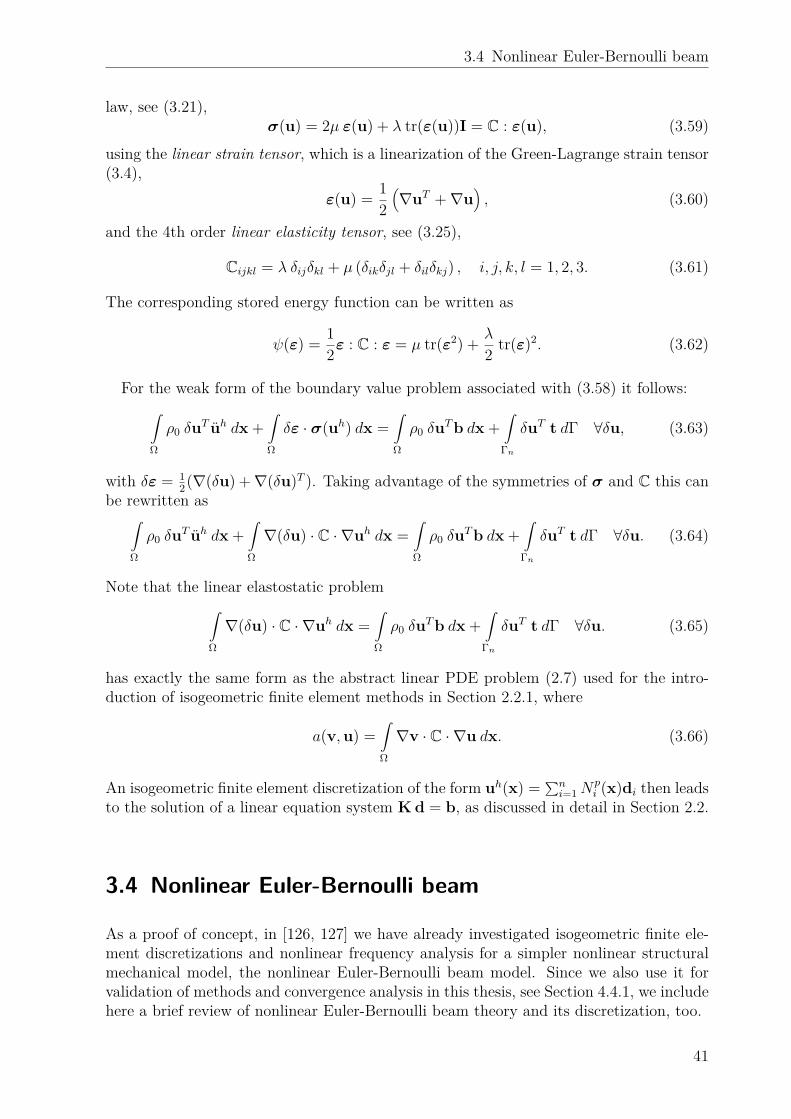
3.4 Nonlinear Euler-Bernoulli beam
law, see (3.21),σ(u) = 2µ ε(u) + λ tr(ε(u))I = C : ε(u), (3.59)
using the linear strain tensor, which is a linearization of the Green-Lagrange strain tensor(3.4),
ε(u) = 12(∇uT +∇u
), (3.60)
and the 4th order linear elasticity tensor, see (3.25),
Cijkl = λ δijδkl + µ (δikδjl + δilδkj) , i, j, k, l = 1, 2, 3. (3.61)
The corresponding stored energy function can be written as
ψ(ε) = 12ε : C : ε = µ tr(ε2) + λ
2 tr(ε)2. (3.62)
For the weak form of the boundary value problem associated with (3.58) it follows:∫Ω
ρ0 δuT uh dx +∫Ω
δε · σ(uh) dx =∫Ω
ρ0 δuTb dx +∫
Γn
δuT t dΓ ∀δu, (3.63)
with δε = 12(∇(δu) +∇(δu)T ). Taking advantage of the symmetries of σ and C this can
be rewritten as∫Ω
ρ0 δuT uh dx +∫Ω
∇(δu) · C · ∇uh dx =∫Ω
ρ0 δuTb dx +∫
Γn
δuT t dΓ ∀δu. (3.64)
Note that the linear elastostatic problem∫Ω
∇(δu) · C · ∇uh dx =∫Ω
ρ0 δuTb dx +∫
Γn
δuT t dΓ ∀δu. (3.65)
has exactly the same form as the abstract linear PDE problem (2.7) used for the intro-duction of isogeometric finite element methods in Section 2.2.1, where
a(v,u) =∫Ω
∇v · C · ∇u dx. (3.66)
An isogeometric finite element discretization of the form uh(x) = ∑ni=1N
pi (x)di then leads
to the solution of a linear equation system K d = b, as discussed in detail in Section 2.2.
3.4 Nonlinear Euler-Bernoulli beam
As a proof of concept, in [126, 127] we have already investigated isogeometric finite ele-ment discretizations and nonlinear frequency analysis for a simpler nonlinear structuralmechanical model, the nonlinear Euler-Bernoulli beam model. Since we also use it forvalidation of methods and convergence analysis in this thesis, see Section 4.4.1, we includehere a brief review of nonlinear Euler-Bernoulli beam theory and its discretization, too.
41

3 Isogeometric finite elements in nonlinear elasticity
q(x)
f(x)x, u1
z, u3
x, u1z, u3
u0(x) w0(x)
Figure 3.4: Unsupported beam under external forces line load q and line-edge load f withtransverse deformation w0 and longitudinal deformation u0 of neutral axis
x
z∆x
q(x)
dwdx
Nxx
Nxx + ∆NxxMxx
Mxx + ∆Mxx
VV + ∆V
Figure 3.5: Internal forces and moments on an infinitesimal beam segment
3.4.1 Nonlinear Euler-Bernoulli beam model
A nonlinear beam model based on Euler-Bernoulli hypothesis and von Karman strains ispresented in detail in [20, 87, 95]. This theory, which is suitable for transverse deforma-tions with small strains and moderate rotations, will be briefly summarized using [95] asmain reference.
The displacement field (u1, u2, u3) along coordinate axis (x, y, z) is expressed by theaxial and transversal displacements of the neutral axis u0(x) and w0(x), see Figure 3.4:
u1 = u0(x)− z w′0(x), u2 = 0, u3 = w0(x). (3.67)
From the general definition of strains
εij = 12
(∂ui∂xj
+ ∂uj∂xi
)+ 1
2
3∑k=1
∂uk∂xi
∂uk∂xj
, (3.68)
only the 00- resp. xx-component of the moderately nonlinear von Karman strain is con-sidered
εxx = u′0 + 12w′0
2 − z w′′0 = ε0xx + z ε1
xx, (3.69)
with the axial strain ε0xx and curvature ε1
xx:
ε0xx = u′0 + 1
2w′0
2, ε1
xx = −w′′0 . (3.70)
From the linear constitutive law, i.e. Hooke’s law, for the stress σxx = Eεxx of anisotropic beam with Young’s modulus E, cross section area A and second moment of
42

3.4 Nonlinear Euler-Bernoulli beam
area I, we obtain the internal force in x-direction Nxx and the internal bending momentaround y-axis Mxx,
Nxx = EA ε0xx, Mxx = EI ε1
xx. (3.71)
The equilibrium of internal forces and moments with axial and transversal externalforces f(x) and q(x) applied on an infinitesimal beam segment ∆x (see Figure 3.5) andtaking the limit ∆x→ 0 leads to the governing equations
−N ′xx = f(x),− (Nxx w
′0)′ −M ′′
xx = q(x).(3.72)
Inserting equations (3.70) and (3.71) into (3.72) then results in the differential equationsfor the bending of a nonlinear Euler-Bernoulli beam, depending on axial and transversaldeformations u0 and w0:
−[EA
(u′0 + 1
2w′0
2)]′
= f(x),
−[EA
(u′0 + 1
2w′0
2)w′0
]′−[−EI w′′0
]′′= q(x).
(3.73)
3.4.2 Isogeometric finite element discretization
For a finite element discretization of the nonlinear beam formulation we need the weakform of governing equations (3.72) resp. (3.73). According to [95] these will be deriveddirectly from the strong form (3.72) using the method of weighted residuals, i.e. multi-plying the equations with test functions v1 resp. v2, taking the integral over the length Lof the beam and applying integration by parts once resp. twice:
L∫0
Nxx · v′1 dx =L∫
0
f · v1 dx+ [Nxx · v1]L0 ,
L∫0
−Mxx · v′′2 + w′0 ·Nxx · v′2 dx =
L∫0
q · v2 dx+ [(M ′xx + w′0 ·Nxx) · v2]L0 + [Mxx · v′2]L0 .
(3.74)
The deformations u0 and w0, as well as test functions v1 and v2 must be included inappropriate function spaces Su,Sw,Vu,Vw and satisfy prescribed deformation boundaryconditions [62].
To solve the weak equations (3.74), Galerkin discretization is applied, i.e., the problemis solved on a mesh Ωh with finite-dimensional function spaces Shu ⊂ Su, Shw ⊂ Sw, Vhu ⊂Vu, Vhw ⊂ Vw defined on Ωh. Then u0 and w0 can be expressed as
u0(x) =n∑i=1
uiNpi (x), w0(x) =
n∑i=1
wiNpi (x) (3.75)
with Npi i=1,...,n being a spline basis of Shu and Shw.
43

3 Isogeometric finite elements in nonlinear elasticity
Inserting these representations into (3.74) leads to the nonlinear systemn∑j=1
K11ij uj +
n∑J=1
K12iJ (w0) wJ = b1
i , i = 1, . . . , n,
n∑j=1
K21Ij (w0) uj +
n∑J=1
K22IJ(w0) wJ = b2
I , I = 1, . . . , n,(3.76)
with stiffness matrices and force vectors
K11ij =
L∫0
EA Npi′ Np
j′ dx,
K12iJ (w0) = 1
2
L∫0
EA w′0 Npi′ Np
J′ dx,
K21Ij (w0) =
L∫0
EA w′0 NpI′ Np
j′ dx = 2 K12
jI ,
K22IJ(w0) =
L∫0
EI NpI′′ Np
J′′ dx+ 1
2
L∫0
EA w′′0 NpI′ Np
J′ dx,
b1i =
L∫0
f(x) Npi dx + Qi,
b2I =
L∫0
q(x) NpI dx + QI .
(3.77)
and Qi, QI being boundary terms derived from (3.74). More details can be found in [95].Now (3.77) can be condensed to the following nonlinear equation system for control pointdeformations d, with deformation-dependent stiffness matrix K = K(d) and force vectorb:
d =(
uw
), K(d) =
(K11 K12
K21 K22
), b =
(b1
b2
), (3.78)
f(d) = K(d) d = b. (3.79)
This nonlinear system of equations has the same structure as (3.53) and can be solvedusing Newton’s method as in Algorithm 1 to compute the static displacement of the beam.
Computational applications and convergence studies for static displacements of thenonlinear Euler-Bernoulli beam with isogeometric finite element discretization, i.e. ex-amples for the solution of (3.79) were computed and discussed in [126, 127]. Results andnumerical convergence analysis for nonlinear frequency analysis were also obtained in thescope of [126, 127] and are presented here in Section 4.4.1.
44

3.5 Computational applications
-t
t
sy
sx
sx
uz
t lr
xyz
(a) Geometry and dimensions of cylinder (b) Deformed cylinder colored by Cauchy stress σyz
Figure 3.6: Geometry and deformation of thick cylinder
3.5 Computational applications
With the computational examples presented in this section we want to validate the im-plementation of our isogeometric finite element discretization of 3-dimensional static non-linear elasticity with large deformations and nonlinear constitutive laws.
3.5.1 Large deformation of thick cylinder
As a first benchmark for the validation of the solution of the nonlinear elastostatic problemusing isogeometric finite elements we take the large deformation of a thick cylinder. Thisproblem was already investigated in [84] to show the advantages of isogeometric comparedto Lagrangian finite elements.
Due to symmetry, the cylinder can be modeled as a quarter cylinder, which is displayedin Figure 3.6(a). The geometrical parameters of the quarter cylinder are inner radius r =0.08 m, thickness t = 0.02 m and length l = 0.15 m. This geometry can be parameterizedexactly as a NURBS volume, using quadratic NURBS in circumferential direction (u) andlinear B-Splines in thickness (v) and length direction (w).
For the analysis, parameters of Neo-Hookean material are chosen the same as in [84]:E = 16.8 kPa, ν = 0.4 and ρ = 470.0 kg/m3. Opposing surface loads are applied witht = (0, 0, 235.0)T Pa (Figure 3.6(a)) and cause a very large compression of the quartercylinder, as can be seen in Figure 3.6(b).
For the validation of our implementation we refine the spline parameterization of ge-ometry for the analysis and obtain a mesh with p = (4, 4, 3), ` = (16, 8, 1), n = 3168.Then we compute the deformation field and evaluate stresses. In Figure 3.6(b) the de-formed cylinder is visualized and colored by the values of Cauchy stress σyz. These resultscorrespond optically very well with the ones obtained in [84].
Furthermore, we carry out a small convergence study for k-refinement of the isogeomet-ric analysis mesh. The load is decreased on 100 instead of 235 Pa in order to ensure conver-gence of Newton iterations and guarantee a realistic deformation without self-penetrationof the cylinder. k-refinement is performed to obtain degree p = 2, 3 in all three parameter
45

3 Isogeometric finite elements in nonlinear elasticity
10−2 10−110−4
10−3
10−2
10−1
100
mesh size parameter h
rela
tive
erro
rsC2 h
2
C3 h3
C4 h4
linearp = 2, rel. L2
p = 2, rel. H1
p = 3, rel. L2
p = 3, rel. H1
nonlinearp = 2, rel. L2
p = 2, rel. H1
p = 3, rel. L2
p = 3, rel. H1
Figure 3.7: Convergence of relative errors in L2- and H1-norm for linear and nonlinearlarge deformation analysis of thick cylinder. k-refinement was performed toobtain degree p = 2, 3 and mesh size h of the parameterization
directions of the mesh. For h-refinement the mesh size parameter depends on the numberof elements and the geometry. It is computed as:
h = maxπ
2r + t
`u,l
`v,t
`w
. (3.80)
For the comparison we evaluate the relative errors of numerical solutions uh in L2- andH1-norm:
rel. L2 :‖u∗ − uh‖L2(Ω)
‖u∗‖L2(Ω), rel. H1 :
‖u∗ − uh‖H1(Ω)
‖u∗‖H1(Ω), (3.81)
where we take numerical solution for the maximally refined mesh with p = (3, 3, 3), ` =(16, 16, 2), n = 10830 as reference solution u∗.
Results of the convergence study are shown in Figure 3.7. We can observe roughly theexpected convergence rates of order p + 1 for the L2- and order p for the H1-norm forboth linear and nonlinear analysis. Until convergence criteria of the Newton’s methodare met in the nonlinear case, i.e. a relative error of residual of 10−5 and relative error ofdisplacement update of 10−6, 7-9 iterations are needed.
With this cylinder example we have validated the implementation of our isogeometricfinite element discretization of nonlinear elasticity by a comparison with the results of[84] and a convergence study.
3.5.2 TERRIFIC Demonstrator as multi-patch example
The so-called “TERRIFIC Demonstrator” is a mechanical part which was introducedwithin the European project “TERRIFIC” [53] to show an isogeometric CAE workflow
46

3.5 Computational applications
(a) geometry in CAD system (b) IGA-suitable multi-patch parameterization
Figure 3.8: Geometry of the TERRIFIC Demonstrator as design in a CAD system (a) andas an analysis-suitable multi-patch volume model (b). Patches are highlightedin different colors; boundaries Γu and Γn, as well as evaluation point E, arealso shown in (b)
from design, over analysis to manufacturing. It was designed in a CAD system (Fig-ure 3.8(a)), an IGA-suitable NURBS volume parameterization was generated for me-chanical simulation (Figure 3.8(b)), and also other models for dip-paint simulation andcomputer-aided manufacturing were derived. Acknowledgement for the design goes toStefan Boschert from Siemens Corporate Technology in Munich and for the multi-patchparameterization to Vibeke Skytt from SINTEF in Oslo.
The TERRIFIC Demonstrator serves also as a realistic, industrial-scale application ofthe methods developed within this thesis. The isogeometric volume parameterizationconsists of 15 patches of quadratic B-Spline volumes, with a total of 6,474 control pointsand 19,422 DOFs. When multi-patch coupling with Lagrangian multipliers is used, theisogeometric finite element discretization of the model has 22,914 DOFs, otherwise whenelimination is used, it is only 15,930 DOFs.
Now we want to compare the results of both types of multi-patch constraint implemen-tations for static linear and nonlinear analysis. We choose St. Venant-Kirchhoff materiallaw with the following material parameters:
E = 74.0 GPa, ν = 0.33, ρ = 2800 kg/m3. (3.82)
As boundary conditions we take a clamping of the right bore hole in Figure 3.8(a) by azero Dirichlet condition at Γu and a surface traction on the left bore hole as a Neumannboundary condition on Γn:
u = 0 on Γu,t = (60.0, −42.0, 0.0)T MPa on Γn.
(3.83)
Running the isogeometric finite element simulations, we find that the results of bothmulti-patch implementations are equal up to at least 12 significant digits for linear andnonlinear analysis for all quantities observed, which are displacement at evaluation pointE in Figure 3.8(b), L2- and H1-norms of displacement field, and potential energy. Thedifferent constraint implementation strategies do not have an influence on assembly times,but of course on the solution time of the linear system. Here it is around 3-times faster
47

3 Isogeometric finite elements in nonlinear elasticity
(a) Colored by displacement magnitude in m
(b) Colored by von Mises stress in Pa
Figure 3.9: Linear (left) and nonlinear (right) deformation of TERRIFIC Demonstrator.Linear analysis over-estimates displacements (a) and stresses (b) more than20% compared to nonlinear results
for elimination than for Lagrangian multipliers, since the linear system is smaller and hasbetter properties, i.e. it is not a saddle-point problem.
Simulation results for the static linear and nonlinear elasticity computations are visu-alized in Figure 3.9, where the deformed structure is plotted and colored by values ofdeformation magnitude 3.9a and von Mises stress 3.9b. Even though the difference be-tween linear and nonlinear analysis might not look significant, the comparison in Table3.1 shows that quantities such as deformation at evaluation point E, L2- and H1-normsof displacement, and potential energy deviate more than 20% and thus justify the use ofnonlinear analysis methods.
In Figure 3.10 it can be noticed that unphysical high stress peaks occur at indentationsin the bending area of the part. These peaks appear for linear and nonlinear analysis, andare caused by a bad parameterization, which is near-singular at the highlighted positionson the boundaries, i.e. det(dx/dξ) ≈ 0. This is not so much a problem for the analysisitself, since quadrature points are located off the boundaries, but for the postprocessingwith strain and stress evaluation. However, it shows both the difficulty of obtainingparameterizations for realistic geometries and the need for development of sophisticatedmethods (see Section 2.3.1).
Altogether, with this computational example we have validated the two alternativeimplementations of multi-patch constraints also for nonlinear elasticity. Furthermore wehave seen that near-singular parameterizations may cause problems for stress evaluation
48

3.6 Summary
ux [m] uy [m] uz [m] Epot [J] ‖u‖L2 ‖u‖H1
linear 0.0183 0.0086 0.0018 1.23·103 2.03·10−4 1.89·10−3
nonlinear 0.0142 0.0066 0.0011 9.80·102 1.53·10−4 1.47·10−3
nonl./lin. 77.4% 76.0% 57.3% 79.4% 75.3% 77.8%
Table 3.1: Comparison of simulation results for linear and nonlinear deformation anal-ysis of TERRIFIC Demonstrator. Deviations of more than 20% show thatlinearization is not accurate and justify the use of nonlinear analysis
Figure 3.10: Unphysical high stress peaks, which occur at indentations in the bendingarea of the part, are highlighted in purple circles. They are caused by a bad,near-singular geometry parameterization
and should be avoided. However, this is an issue of the generation of analysis-suitableparameterizations and beyond the scope of this work.
3.6 Summary
We have dedicated this chapter to the spatial discretization of nonlinear elasticity prob-lems using the isogeometric finite element method, which was already introduced in Chap-ter 2.
We have started with an introduction to fundamentals of 3-dimensional continuummechanics. As we aim at the simulation of vibrations of rubber components, also visco-hyperelastic constitutive laws with frequency-dependent material parameters need to beconsidered.
Then we have explained the application of the isogeometric finite element method tothe discretization of the nonlinear continuum mechanics problem. The displacements ofstatic deformations can then be computed using a Newton’s method.
49

3 Isogeometric finite elements in nonlinear elasticity
For the evaluation of nonlinear analysis, we need to compare the results with linearelasticity, which is only valid for small displacements. Furthermore, we have introducedthe simpler structural model of the nonlinear Euler-Bernoulli beam, which also serves forvalidation and benchmarking of our methods.
Finally, we have used computational applications to validate the implementation of iso-geometric finite elements for nonlinear elasticity and confirmed the convergence proper-ties. With the TERRIFIC Demonstrator example, we have proven the ability to simulaterealistic geometries as isogeometric multi-patch models.
50

4 Nonlinear frequency analysis
Having introduced the problem formulation of nonlinear structural dynamics and thespatial discretization using isogeometric finite elements in preceding Chapter 3, we nowtarget the topic of frequency analysis.
We start with a brief review of methods for linear frequency analysis, i.e. modal analysisof eigenfrequencies and eigenmodes, and direct frequency response to harmonic excitationsin Section 4.1. Thereafter we give a general survey of methods for nonlinear frequencyanalysis in Section 4.2. Then we introduce in detail the method of harmonic balance fornonlinear steady-state frequency response analysis for periodic excitations, its applicationin nonlinear mechanics and its properties in Section 4.3. Finally, in Section 4.4 we discusscomputational examples for nonlinear frequency analysis using harmonic balance andisogeometric finite element discretizations.
4.1 Overview of linear frequency analysis methods
In Section 3.3 we have introduced the linear elasticity problem, which reads, see (3.58),
ρu− div σ(u) = ρb ∀x ∈ Ω, t ∈ [0, T ], (4.1)
in the strong form. After (isogeometric) finite element discretization we have a system ofN coupled linear ordinary differential equations for control point displacements d:
M d(t) + K d(t) = b(t) ∀t ∈ [0, T ]. (4.2)
Furthermore, in vibration problems we have periodicity conditions for the displacementvectors in time:
d(0) = d(T ) ∧ d(0) = d(T ). (4.3)
In structural dynamics very often velocity-dependent damping is introduced in thediscretized equation of motion:
M d(t) + C d(t) + K d(t) = b(t) ∀t ∈ [0, T ]. (4.4)
The damping term C d can relate to viscose effects in the material, internal or externalfriction and leads to dissipation of energy [130]. Using d = v, (4.4) can also be rewritten
51

4 Nonlinear frequency analysis
as a first order linear symmetric ODE system:(M 00 −K
)(vd
)+(
C KK 0
)(vd
)=(
b0
). (4.5)
A typical choice of the damping matrix is so-called Rayleigh or modal damping, whereC = αM + βK. The Rayleigh coefficients α, β > 0 have to be chosen carefully and fit tothe material used and also to a frequency range where they are valid [62].
When linear viscoelastic materials are employed, and can be described using the Kelvin-Voigt model, see Section 3.1.4, the damping matrix takes the form C = ηK, where η isthe loss factor.
4.1.1 Modal analysis and eigenfrequencies
Modal analysis plays an important role in structural and mechanical engineering, sinceeigenfrequencies and eigenforms are important characteristics of the dynamical behavior ofstructures. Solutions of the generalized eigenvalue problem indicate resonance frequenciesthat should be avoided for forced vibrations [62].
Linear eigenvalue problem
From the equation of motion (4.2) with b(t) ≡ 0 and periodicity conditions (4.3) bymaking the ansatz d(t) = φk e
iωkt one can derive the well-known eigenvalue problem
ω2k M φk = K φk, k = 1, . . . , N, (4.6)
for the N linear natural frequencies ωk > 0, resp. eigenfrequencies λk = ω2k, and corre-
sponding eigenvectors or eigenmodes φk 6= 0 [39, 62]. Using Λ = diag(ω21, . . . , ω
2N) and
Φ = (φ1, . . . ,φN), the eigenvalue problem can be written as:
Λ M Φ = K Φ. (4.7)
Typically the eigenmodes are normalized such that
ΦT M Φ = I and ΦT K Φ = Λ. (4.8)
As we have already outlined in Section 2.2.2, higher smoothness of isogeometric splinediscretizations is particularly advantageous compared to standard C0 finite elements forthe solution of eigenvalue problems [42, 76].
Complex eigenvalue problem
When damping is included, the ansatz d(t) = φk eλkt is made with complex λk and it
follows that v(t) = λk φk eλkt =: ψk e
λkt and thus
λk
(−M 0
0 K
)(ψk
φk
)=(
C KK 0
)(ψk
φk
), k = 1, . . . , 2N. (4.9)
52

4.1 Overview of linear frequency analysis methods
Algorithm 2 Iterative eigenvalue problem for frequency-dependent materials1: for k = 1, 2, . . . do2: Solve: ω0
k2 M φ0
k = K(0) φ0k
3: Initialization: s← 04: repeat5: s← s+ 16: Assembly: Ks ← K(ωs−1
k )7: Solve: ωsk
2 M φsk = Ks φsk
8: until |(ωsk − ωs−1k )/ωsk| < ε
9: Return values: ωk = ωsk, φk = φsk
10: end for
This gives N pairs of complex-conjugate eigenvalues of the form
k = 1, . . . , N :
λ2k−1 = −ζkωk − iωk√
1− ζ2k ,
λ2k = −ζkωk + iωk√
1− ζ2k .
(4.10)
where ωk are again the natural frequencies and ζk the modal damping ratios, which canbe computed from λ2k−1 = αk − iβk and λ2k = αk + iβk:
ωk =√α2k + β2
k , ζk = −αk/ωk, k = 1, . . . , N. (4.11)
The damped and undamped natural frequencies are equal when the matrix KM−1C issymmetric [79], which is the case for Rayleigh and viscoelastic Kelvin-Voigt damping:
C = αM + βK ⇒ KM−1C = αK + βKM−1K,
C = ηK ⇒ KM−1C = ηKM−1K.(4.12)
Here symmetry is obvious since K and M are symmetric.
Frequency-dependent eigenvalue problem
Viscoelastic materials, as introduced in Section 3.1.4, may have strongly frequency-depen-dent properties constants that should be taken into account also for the solution of eigen-value problems:
ω2k M φk = K(ωk) φk, k = 1, . . . , N. (4.13)
In [123] an iterative approach for the solution of the linear eigenvalue problem with K =K(ω) was suggested to determine the frequency-dependent natural frequencies ωk andeigenmodes φk, which is presented here in Algorithm 2.
In general the stiffness matrix K(ω) depends on two frequency-dependent parameters,Young’s modulus E(ω) and Poisson’s ratio ν(ω). If ν is assumed as constant, only E(ω)remains as a linear parameter:
K(ω) = E(ω)E(0) K(0). (4.14)
53

4 Nonlinear frequency analysis
In this case it is not necessary to reassemble K(ω) in every iteration step, it can just beobtained by scaling of K(0). Furthermore, as it is shown in Appendix A.1, the frequency-dependent eigenvalue problem even reduces to φk = φk and the solution of the followingscalar nonlinear equation for ωk:
ωk = ωk
√E(ωk)E0
. (4.15)
However, in situations where K is obtained from an isogeometric multi-patch finiteelement discretization, see Section 2.3.1, K(ω) = E(ω)
E(0) K(0) is not necessarily true for theglobal stiffness matrix, but maybe only for a patch submatrix with frequency-dependentmaterial it is Ki(ω) = Ei(ω)
Ei(0) Ki(0). Then the above-mentioned simplification as scalar non-
linear equation for ωk cannot be used anymore, but at least in Algorithm 2 the submatrixcan be scaled and need not be reassembled.
Also the complex eigenvalue problem with damping from (4.9) can be formulated forfrequency-dependent materials and an iteration similar to Algorithm 2 can be carried outto compute natural frequencies and damping ratios.
Modal participation factors
For systems with several hundreds of thousands or even millions of degrees of freedom itis very costly to compute numerical solutions of the generalized eigenvalue problem, seesubsequent Section 4.1.1. Thus typically only a fraction of the smallest eigenfrequenciesand corresponding modes is computed [62].
Effective modal masses or modal participation factors are a measure of the significanceof modes for the vibration of a system and may provide a guideline for how many andwhich modes should be computed to accurately capture the vibrational behavior of asystem, or which modes should be included in a reduction basis when a system is reducedonto its modes, see Chapter 5.
Modal participation factors are computed with respect to an influence vector r ∈ RN .Typically, it is r ≡ 1, or to differentiate among spatial directions it can be chosen rx =(1, 0, 0, 1, 0, 0, . . . , 1, 0, 0)T and ry, rz analogous.
Then for a mass-normalized eigenmode φk with φTkMφk = 1, the modal participationfactor Γk and effective modal mass meff,k are defined as
Γk = φTk M r, meff,k = Γ2k. (4.16)
When r ≡ 1 it holds for the effective modal masses and the total mass of the system mtot:
N∑k=1
meff,k = 3mtot. (4.17)
Numerical solution of generalized eigenvalue problems
Typically generalized eigenvalue problems like (4.6) are rewritten as standard eigenvalueproblems [13, 124]:
λkφk = M−1K φk, k = 1, . . . , N, (4.18)
54
4.1 Overview of linear frequency analysis methods
which requires M to be positive definite, i.e. invertible. Then, an iterative numericalalgorithm for the approximate solution of the symmetric standard eigenvalue problem forsome k has to be chosen from a wide range of methods, including Householder-QR-inverse,generalized Jacobi, Krylov subspace or determinant search methods [13, 113].
In multi-patch problems with Lagrangian multipliers, see Section 2.3.2, the generalizedeigenvalue problem (4.6) takes the form
λk M∗ φ∗k = K∗ φ∗k, k = 1, . . . , N,
⇔ λk
(M 00 0
)(φkψk
)=(
K BT
B 0
)(φkψk
), k = 1, . . . , N,
(4.19)
where the matrix M∗ is only positive semi-definite. A static condensation, as for exampleused for lumped mass matrices with zero diagonal entries, is not possible here, since the(2,2)-block of K∗ is also zero. Instead, it must be reformulated as a standard eigenvalueproblem by inverting K∗:
1λkφ∗k = K∗−1M∗ φk, k = 1, . . . , N. (4.20)
4.1.2 Direct frequency response
Another means of linear frequency analysis, which is also available in most FEA software,is the so-called direct frequency response (DFR) method for computing the steady-stateresponse of a structure subject to harmonic loading. The method is sometimes also referedto as harmonic response analysis or simply harmonic analysis, as the external force vectoris of the form
b(t) = bc cosωt+ bs sinωt, ∀t ∈ [0, T ], (4.21)
where ω is the fundamental frequency of the excitation and T = 2π/ω the period ofvibration. Then, the deformation vector is also expressed as a sum of cosine and sinefunctions
d(t) = dc cosωt+ ds sinωt, ∀t ∈ [0, T ], (4.22)
which leads to the following form of the discretized equation of motion (4.4):(−ω2 M dc + ω C ds + K dc − bc
)cosωt +(
−ω2 M ds − ω C dc + K ds − bs)
sinωt = 0 ∀t ∈ [0, T ].(4.23)
Both time-independent terms in brackets have to be zero for (4.23) to fulfilled for allt ∈ [0, T ], which leads to the following 2N -sized system of equations:(
−ω2 M + K ω C−ω C −ω2 M + K
)(dcds
)=(
bcbs
). (4.24)
Typically (4.24) is solved over a range of frequency values ω in order to obtain thefrequency response curves, which show vibration amplitudes and phase at a certain eval-uation point on the structure, or the values of kinetic or potential energy. For every time
55

4 Nonlinear frequency analysis
t ∈ [0, T ], the kinetic and potential energy are:
Ekin(t) = 12 d(t)TM d(t), Epot = 1
2 d(t)TK d(t) = 12 d(t)Tb(t). (4.25)
Integrating these expressions over the time interval [0, T ] leads to the total energies of oneperiod of vibration:
Ekin = 1T
T∫0
12 d(t)TM d(t) dt
= ω
2πω2
2
T∫0
sin2 ωt dTc M dc + cos2 ωt dTs M ds − 2 sinωt cosωt dTc M ds
dt
= ω2
4(dTc M dc + dTs M ds
),
Epot = 1T
T∫0
12 d(t)TK d(t) dt
= ω
2π12
T∫0
cos2 ωt dTc K dc + sin2 ωt dTs K ds + 2 cosωt sinωt dTc K ds
dt
= 14(dTc K dc + dTs K ds
).
(4.26)
4.2 Survey of nonlinear frequency analysis methods
The solution of eigenvalue problems and direct frequency response are two standard meth-ods in engineering practice for linear frequency and vibration analysis of structures andimplemented in almost every commercial and open-source finite element software for struc-tural analysis. However, nonlinear vibration analysis is a much more difficult and un-conventional task, which is lacking efficient numerical methods and implementations forlarge-scale applications in structural dynamics. For a general summary of methods fornonlinear oscillation resp. frequency analysis we refer to [86, 87, 117].
To give an overview of methods for nonlinear frequency analysis methods in structuraldynamics, we recall the semi-discretized equation of motion with periodicity boundaryconditions
M d(t) + C d(t) + f(d(t), d(t)) = b(t) ∀t ∈ [0, T ],d(0) = d(T ), d(0) = d(T ).
(4.27)
This is a nonlinear ordinary differential equation system, in contrast to the linear orlinearized equation of motion in (4.4), which we have treated so far in Section 4.1. Thesystem arises from the isogeometric finite element discretization of nonlinear continuummechanics with large deformations and visco-hyperelastic material models, as we havederived it in Section 3.2, (3.45).
56

4.2 Survey of nonlinear frequency analysis methods
4.2.1 Nonlinear counterparts of eigenmodes
We review two kinds of extensions or counterparts of the concept of linear eigenmodes,which can be used to describe vibrational behavior of nonlinear systems: tangent modesand nonlinear normal modes. Both can also be employed in reduced-order modeling ofnonlinear systems, see later Section 5.1.
Tangent modes
Tangent modes are the eigenmodes one obtains from the solution of an updated eigenvalueproblem with the tangent stiffness for the current deformation state [96, 112]:
ω2k M φk = KT (φk) φk. (4.28)
While linear eigenmodes in (4.6) are independent of their scaling, the tangent stiffnessmatrix KT (φk) depends on the size and scaling of the tangent mode φk, and thus alsoon the mode itself. Tangent modes φαk can be computed depending on a parameter α,which could be for example the norm of the mode α = ‖φαk‖, or the value of a specificcomponent α = φαki. Defining φ0
k for α = 0 as the linear eigenmode, one can set up ahysteresis for computing φαk and observe the nonlinear dependency of the tangent modeon the parameter α.
We compute tangent modes for example in the numerical application of a thick cylinderin Section 4.4.2 and Figure 4.6.
Nonlinear normal modes
Another nonlinear counterpart of linear eigenmodes, which are sometimes also calledlinear normal modes, are nonlinear normal modes (NNMs). They were first introducedfor single-DOF and multiple-DOF systems in [103, 108, 122]. In this context a soundtheoretical foundation was established, including existence, stability and bifurcation ofNNMs.
However, the concept of NNMs was restricted to weakly nonlinear systems, where thenonlinearity depends on a perturbation parameter ε. Only since 1990’s NNMs have beenalso investigated in nonlinear structural dynamics with stronger nonlinearities [72, 92].
NNMs can be defined either as “a vibration in unison of the system (i.e., a synchronousperiodic oscillation)” [92] or as “two-dimensional invariant manifold in phase space” [92],which depend on the energy of the system [103, 108] – very similar to tangent modesdepending on the scaling parameter α. For systems with only few DOFs they are com-puted by an energy-based formulation, an invariant manifold approach using two mastercoordinates, the multiple scales method or a truncated Fourier series ansatz for the timedomain [72, 92]. For larger systems numerical techniques must be used, such as numericalintegration, also using shooting methods, the so-called asymptotic-numerical method, orthe autonomous version of the harmonic balance method, see the following Section 4.3.
Tangent modes are relatively simple to compute as iterative solutions of the eigenvalueproblem or using a continuation of the parameter α, but they do not account for internalresonances and can only be determined in the neighborhood of a linear eigenfrequency
57

4 Nonlinear frequency analysis
resp. eigenmode. The concept of NNMs is therefore more general, but numerical algo-rithms for their computation are more complex. For instance, an autonomous version ofharmonic balance method (see Section 4.3) can be used.
4.2.2 Steady-state response by time integration
The problem of steady-state response to harmonic loading is the nonlinear counterpartof linear DFR, see Section 4.1.2. In engineering practice it is typically solved by timeintegration of the initial value problem (4.27) [20, 54, 130], also in the IGA context [39].
A suitable time integration method, such as explicit or implicit Euler methods, New-mark, Runge-Kutta, or BDF, has to be selected [20, 113, 130]. Since all of these methodsrely on the approximation of time derivatives of displacements, i.e. velocities, the time-step size ∆t is a critical quantity. It has to be chosen carefully with ∆t T = 2π/ωin order to guarantee the accuracy of the method and be able to capture the oscillatorybehavior of loads and displacements in wave propagation problems [130].
Then, time integration must be carried out over many periods T until a steady-stateof motion is reached. For strongly damped systems this is the case much faster thanfor undamped or only lightly damped systems. This indicates that numerical dampingmight be needed for stability of the integration method for a conservative system, whereno physical dissipation is included. But then it introduces a phase shift and inaccuracyof the solution, since angular momentum and energy might not be conserved [130].
Shooting methods can also be employed to solve (4.27) with time integration as aboundary value problem instead of an initial value problem [54, 113].
Due to the above-mentioned disadvantages of time integration methods, high compu-tational effort due to small step size and integration over many cycles, we prefer a differ-ent method for the computation of steady-state response, namely the harmonic balancemethod.
4.3 The harmonic balance method
The Harmonic Balance Method (HBM) is a means for the approximation of solutions ofperiodic nonlinear ODE systems, which is based on a truncated Fourier series expansionof the solution. It was originally developed by W. Szemplinska-Stupnicka in 1960’s asa semi-analytical method and applied to systems with only few DOFs [115, 116, 117].Sometimes it is also called multi-harmonic balance or describing function method.
Nowadays it is widespread in application to electrical circuits with nonlinear compo-nents [31, 54, 55, 106], or also for electromagnetic problems [9]. In structural dynamics, ithas been mainly applied to FE discretizations of lower-dimensional beam and shell models[80, 81, 87, 100, 98, 99].
HBM can be used to compute either the solution of a nonlinear, self-excited system,i.e. a nonlinear normal mode, see Section 4.2.1, or to determine steady-state response toa periodic external force, as an alternative to time integration presented in Section 4.2.2[87].
58

4.3 The harmonic balance method
4.3.1 Introduction of the method
Here, we apply the harmonic balance method to compute steady-state response of non-linear mechanical systems, which are governed by large deformation visco-hyperelasticity.Starting point is the equation of motion after semi-discretization using isogeometric finiteelements, which was already given in (4.27). It is a nonlinear second-order ODE for thevector of control point displacements d(t) ∈ RN with periodicity conditions:
M d(t) + C d(t) + f(d(t), d(t)) = b(t) ∀t ∈ [0, T ],d(0) = d(T ), d(0) = d(T ).
(4.29)
As mentioned before, periodic external excitations of the structure are considered witha fundamental frequency ω, resp. frequency f = ω/(2π) or period T = 2π/ω, which canbe described as an harmonic series with finite number m∗ of cosine and sine terms:
b(ω, t) = 12b0 +
m∗∑k=1
cos(kωt) bk + sin(kωt) b2m∗−k+1. (4.30)
The response to periodic excitation is expected to be ω-periodic as well and thus thedisplacement vector d(t) of the spatial discretization uh(x, t) = ∑n
i=1Npi (x) di(t) (3.39),
and consequently also the velocities d and accelerations d, are expressed as an harmonicseries, or in other words as a truncated Fourier expansion, with m ≥ m∗ harmonic termsof fundamental frequency ω and amplitudes q =
(qT0 , . . . ,qT2m
)T∈ R(2m+1)N :
d(q, ω, t) = 12q0 +
m∑k=1
cos(kωt) qk + sin(kωt) qk,
d(q, ω, t) =m∑k=1−kω sin(kωt) qk + kω cos(kωt) qk,
d(q, ω, t) =m∑k=1−k2ω2 cos(kωt) qk − k2ω2 sin(kωt) qk,
(4.31)
using the abbreviation k := 2m− k + 1.Substitution of the ansatz for displacements from (4.31) into (4.29) results in a residual
vector:
r(q, ω, t) = M d(q, ω, t) + C d(q, ω, t) + f(d(q, ω, t), d(q, ω, t)
)− b(ω, t). (4.32)
In order to compute the amplitudes qk, Ritz procedure is applied by projecting the residualr onto the basis functions of the frequency domain, which results in a Fourier expansionof the residual r with 2m+ 1 coefficient vectors rj that have to be evaluated to 0 (balanceof the harmonics):
rj(q, ω) = 2T
T∫0
r(q, ω, t) cos(jωt) dt != 0, j = 0, . . . ,m ,
rj(q, ω) = 2T
T∫0
r(q, ω, t) sin(jωt) dt != 0, j = 1, . . . ,m.
(4.33)
59

4 Nonlinear frequency analysis
The nonlinear system of (2m+ 1)N equations given by (4.33), which we abbreviate as
r(q, ω) = 0, (4.34)
has to be solved to determine the amplitudes q and thus obtain the steady-state frequencyresponse of the system.
4.3.2 Implementation aspects
Fourier transform of residual
As mentioned above, the projection of the residual vector r onto harmonic basis functionsin (4.33) equals a Fourier transform, or more precisely a Hartley transform, since ittransforms the real-valued residual onto real-valued coefficients [58].
Thus the numerical evaluation of integrals in (4.33) can be performed as a discreteHartley transform (DHT, [27]) of the residual. First the integrals are transformed onto anon-dimensional time τ = ωt, such that the domain of integration becomes [0, 2π]. Thenthe residual r(q, ω, τ) has to be sampled at equidistant times τj = 2πj
2m+1 , j = 0, . . . , 2mand it becomes:
r0 = r∗02m+ 1 , rj =
r∗j + r∗j2m+ 1 , rj =
r∗j − r∗j2m+ 1 , j = 1, . . . ,m, (4.35)
where
r∗j = r(q, ω, τ0) +2m∑k=1
r(q, ω, τk)√
2 cos(
2πjk2m+ 1 −
π
4
), j = 0, . . . , 2m. (4.36)
Aliasing effects due to undersampling do not occur here, since the highest frequencyof the signal, here the highest harmonic of (4.31), is m, which is smaller than half ofthe sampling rate, which is 2m + 1. Thus Nyquist-Shannon/WKS sampling theorem isfulfilled [26, 90].
Solution using Newton’s method
For given ω, (4.34) is a nonlinear system of (2m+1)N equations in r for the same numberof unknowns q. Thus it can be solved using a Newton’s method, just like Algorithm 1(page 39) for the solution of the static nonlinear elasticity problem.
For that matter also the Jacobian J ∈ R(2m+1)N×(2m+1)N of residual coefficients rj withrespect to amplitudes qk needs to be computed:
J(q, ω) =(drjdqk
(q, ω))j,k=0,...,2m
:
drjdqk
(q, ω) = 2T
T∫0
drdqk
(q, ω, t) cos(jωt) dt, j = 0, . . . ,m ,
drjdqk
(q, ω) = 2T
T∫0
drdqk
(q, ω, t) sin(jωt) dt, j = 1, . . . ,m.
(4.37)
60

4.3 The harmonic balance method
As described above, the integrals in (4.37) are also evaluated using DHT and are thustransformed onto τ = ωt and sampled at times τj. Furthermore, also the Jacobiansdrjdqk
= Jk ∈ RN×N of the residual vector r with respect to amplitude vectors qk need tobe computed:
Jk(q, ω, t) = drdqk
(q, ω, t) =− k2ω2 cos(kωt) M− kω sin(kωt) C + cos(kωt) dfdd
(q, ω, t)
− kω sin(kωt) dfdd
(q, ω, t), k = 0, . . . ,m,
Jk(q, ω, t) = drdqk
(q, ω, t) =− k2ω2 sin(kωt) M + kω cos(kωt) C + sin(kωt) dfdd
(q, ω, t)
+ kω cos(kωt) dfdd
(q, ω, t), k = 1, . . . ,m.(4.38)
Here the terms dfdd(q, ω, t) and df
dd(q, ω, t) refer to the tangent stiffness matrix KT (d, d), see(3.54), and a viscous tangent matrix CT (d, d), which have to be computed and evaluatedfor the current displacement and velocity vectors d(t) and d(t), which depend on theamplitudes q, frequency ω, and time t using (4.31).
Altogether, Newton’s method for the solution of harmonic balance is summarized inAlgorithm 3.
The effort of computing q for a fixed ω using Algorithm 3 is mainly the assembly offorce vectors and tangent matrices for each of the 2m + 1 times τj of the sampling loop(line 8), which has to be repeated for each iteration step s of the Newton-Raphson loop.Furthermore, a bottle neck is the solution of the linear system of size (2m + 1)N in line14, which is addressed with the reduction method proposed in Chapter 5.
Frequency response curves
Response curves (RC) are a wide-spread means of visualizing the frequency response ofsteady-state vibrating systems, also for linear DFR (Section 4.1.2). Typically, the totalamplitude ak and phase φk of one or more harmonics k are evaluated at a specific pointon the structure for fixed ω and plotted over a certain range of frequency. They can becomputed as follows:
ak =√q2k + q2
k, φk = arctan qk
qk, (4.39)
qk cos(kωt) + qk sin(kωt) = ak cos(kωt+ φk). (4.40)
The simplest method for generating response curves and functions is simply to startfrom a fixed ω, compute the response via HBM using Algorithm 3 or DFR, computeamplitude and phase at the evaluation point, and then increment the frequency step bystep [86, 87].
However, nonlinear vibrational behavior usually also includes bifurcations with severalsolution branches and turning points, which makes it necessary to use homotopy resp.continuation methods [1, 57, 86, 97]. Usually an arc-length parameter λ = λ(q, ω) isintroduced, which is incremented instead of frequency increments only, and allows a si-multaneous update of amplitude vector q and frequency ω. Hence Algorithm 3 has to be
61

4 Nonlinear frequency analysis
Algorithm 3 Newton’s method for harmonic balance1: Preassembly: M, C2: Tolerances: εq, εr > 03: Initial guess: q0
4: Initialization: s← 05: repeat6: for j = 0, . . . , 2m do7: Sampling time: τj = 2πj/(2m+ 1)8: Current displacement: d(τj) = qs0/2 +∑m
k=1 cos(kτj) qsk + sin(kτj) qsk
9: Assembly: f(τj)← f(d(τj), d(τj)), b(τj)KT (τj)← KT (d(τj), d(τj)),CT (τj)← CT (d(τj), d(τj))
10: Evaluate residual: r(τj)←M d(τj) + C d(τj) + f(τj)− b(τj)11: Evaluate Jacobians: Jk(τj)← see (4.38), k = 0, . . . , 2m12: end for13: DHT of residual: rs ← DHT(r(τ0), . . . , r(τ2m))14: DHT of Jacobians: J
s
k ← DHT(Jk(τ0), . . . ,Jk(τ2m)), k = 0, . . . , 2m15: Compute update: ∆qs ← Solve J
s ∆qs = −rs
16: Evaluate error: eq ← ‖∆qs‖‖qs‖ , er ← ‖rs‖
‖qs‖
17: Update: qs+1 = qs + ∆qs
18: s← s+ 119: until eq < εq ∧ er < εr
20: Return value: q← qs
modified such that an additional equation for the arc-length parameter and derivativesw.r.t. ω are introduced [106].
4.3.3 Theoretical properties
We apply the harmonic balance method for a time-discretization of the equation of motionof elasticity, which is a hyperbolic, nonlinear PDE boundary value problem and reads inthe continuous form, compare (3.11):
ρ0u(x, t)− div [F S](x, t) = ρ0b(x, t) ∀x ∈ Ω, ∀t ∈ [0, T ],u(x, t) = h(x, t) ∀x ∈ Γu, ∀t ∈ [0, T ],
[F S n](x, t) = t(x, t) ∀x ∈ Γn, ∀t ∈ [0, T ],u(x, 0) = u(x, T ) ∀x ∈ Ω,u(x, 0) = u(x, T ) ∀x ∈ Ω.
(4.41)
Using isogeometric finite elements for the spatial discretization (Section 3.2) and theharmonic balance method for the temporal or frequency domain discretization (Section
62

4.4 Computational applications
4.3.1), it follows that a weak solution of this problem can be expressed by separation ofvariables as
uh(x, t) =n∑i=1
Npi (x)
(12q0,i +
m∑k=1
cos(kωt) qk,i + sin(kωt) qk,i
). (4.42)
Properties of the IGA-FEM discretization have already been outlined in Section 2.2.2.The harmonic balance method is a Fourier spectral method [26], i.e. a Galerkin methodwhere the span of the basis functions is global and ranges over the whole domain. Here,Fourier basis functions cosine and sine are employed on time domain [0, T ], which auto-matically fulfill the periodicity boundary conditions.
It can be shown that the Fourier coefficients of a C∞-continuous function decreaseexponentially [26]. For spectral methods with sufficiently smooth exact solution anddata, this means that the error in approximating the exact solution of a differential orintegral equation is of order O(m−m), where m is the number of spectral basis functions.This so-called exponential convergence of spectral methods such as harmonic balance canbe achieved since m is at the same time the order of the basis functions and the meshparameter is h = O(1/m) [26].
However, we use a Fourier series for the approximation of the solution of a forced vi-bration problem in nonlinear elasticity, where an exact solution and its Fourier seriesexpansion is in general not known. Thus the accuracy of an harmonic balance approxi-mation may highly depend on the number of harmonics m. Nonlinear effects, such as thecubic nonlinearity of large deformation kinematics, nonlinear constitutive laws, internalresonance and coupling of modes, typically cause response in higher harmonics m > m∗
than the highest excited harmonic.In the numerical examples presented in this thesis, we typically use m ≥ 2m∗.
4.4 Computational applications
Having introduced harmonic balance as our prefered method for steady-state nonlinearfrequency response analysis, we want to use some computational examples to verify themethod and examine its properties numerically. In the first application in Section 4.4.1we investigate a sub-harmonic resonance of a nonlinear Euler-Bernoulli beam. We studyconvergence of HBM regarding the isogeometric spatial discretization and also the influ-ence of Fourier series length for the time domain discretization. Then we use the forcedvibration of a thick cylinder as example for 3-dimensional nonlinear elasticity in Section4.4.2. The results of HBM are verified in the comparison to linear DFR and nonlineartangent modes.
4.4.1 Convergence studies for the nonlinear Euler-Bernoulli beam
As a first feasibility study for the use of isogeometric finite element discretizations in com-bination with harmonic balance method for the nonlinear analysis of forced vibrations,we have investigated the nonlinear Euler-Bernoulli beam. Since the beam is a simplifiedstructural model with a one-dimensional parameterization and two displacement com-ponents, see Section 3.4, computational effort of a nonlinear frequency analysis is much
63

4 Nonlinear frequency analysis
L = 1.0 m, A = 0.1 m2, E = 0.2 MPa,I = 0.00081 m−4, r = 0.09 m, ρ = 2000 kg/m3,
p(x, t) = 20 EI r/L3 sin(πx/L) cos(ωt),
p(x)
Figure 4.1: Properties of simply supported beam subject to periodic sinusoidal load
less for the beam than for a 3-dimensional continuum mechanics formulation. Hence itis especially suitable for the investigation of convergence properties of the methods, i.e.of the spatial discretization using IGA and of the time/frequency-domain discretizationwith harmonic balance. The results presented in this section have been obtained withinthe diploma thesis [126] and were published in [127].
The parameters of a simply supported beam subject to a time-periodic, sinusoidal dis-tributed load are given in Figure 4.1. For the error calculation and convergence study wefocus on the mid span of the beam, where sub-harmonic resonance in the third harmonica3 occurs around ω/ω1 ≈ 0.34.
In Figure 4.2 the response curves for degree p = 3 and n = 8, 12 control points aroundω/ω1 ≈ 0.34 are plotted. Fourier series length is fixed at m = 3 and we compare theresponse curves for k-refinement method (IGA) and p-method (FEM). As the curves arehardly distinguishable, in all cases the sub-harmonic resonance in with rapidly growingamplitude a3 is captured. Only for the p-method with ` = 8 a difference to the othercurves is visible, for the other cases the curves match optically very well.
For a more detailed convergence analysis of the spatial discretization with respect top, h = 1/` and continuity, Fourier series length is fixed at m = 3, since the contributionof higher-frequency amplitudes above a3 is very small. The convergence plot in Figure4.3 shows the error in the amplitude of the third harmonic |ah3 − a3| at ω/ω1 = 0.338 forp = 3, 4, 5. As reference solution a3 we take the numerical one obtained from p = 5 anda sufficient number of DOFs with an accuracy of 8 digits (an error of magnitude 10−9
is assumed to be equal to exact solution a3 = 0.20568197 m). The order of convergenceis again O(h2(p−1)), at least for p = 3, but in general the error for the Cp−1 k-method(IGA) is much smaller than for C1-continuous p-method (FEM). This matches the errorestimates obtained for linear modal analysis and the static deformation computation, seeSection 2.2.2.
Now we take a deeper look at the m-convergence, i.e. convergence with respect to thenumber of harmonics or Fourier series length of the harmonic balance discretization. InTable 4.1 the amplitudes a3 at ω/ω1 = 0.336 are given for increasing Fourier series lengthm with IGA and p = 5, ` = 18. Here, ε = |a11
3 − am3 |/|a113 | is the relative error in a3
compared to the value for m = 11, which is also plotted over m in Figure 4.4. It canbe observed that the error decreases very fast with increasing m, which is a sign of theexponential convergence order m−m of harmonic balance. However, not all increments inm contribute to a decrease of ε. The reason is probably that the 5th or 8th harmonicsimply do not contribute to the solution due to the type of nonlinearity.
Altogether, with the nonlinear Euler-Bernoulli beam feasibility study we could showthat the convergence properties of isogeometric finite elements carry over to nonlinearfrequency analysis, i.e. a higher accuracy compared to Lagrangian FE, and also thatthere is a rapid convergence with respect to the Fourier series length m.
64

4.4 Computational applications
0.33 0.332 0.334 0.336 0.338 0.34 0.342 0.344 0.346 0.348 0.350
0.1
0.2
0.3
0.4
0.5
0.6
normalized frequency ω / ω1
rela
tive
ampl
itude
s a
i / r
a1
a3
p=3, l=5, n=8 (IGA)p=3, l=9, n=12 (IGA)p=3, l=3, n=8 (FEM)p=3, l=5, n=12 (FEM)
Figure 4.2: Response curves of beam for C2- (IGA) and C1-continuous (FEM) cubic B-Splines (p = 3) and n = 8, 12 control points. Amplitudes a1 and a3 arenormalized by beam thickness r and shown at sub-harmonic resonance aroundω/ω1 ≈ 0.34
0.01 0.05 0.1 0.5
10−8
10−6
10−4
10−2
100
mesh size h
erro
r |
ah 3 − a
3 |
p=3 (IGA)p=3 (FEM)
h4
p=4 (IGA)p=4 (FEM)
h6
p=5 (IGA)p=5 (FEM)
h8
Figure 4.3: Convergence plot of the error in third harmonic amplitude a3 at ω/ω1 = 0.338using k- (IGA) and p-refinement (FEM) for degrees p = 3, 4, 5 and differentmesh sizes h
65

4 Nonlinear frequency analysis
m 3 4 5 6a3 0.08762534 0.11654205 0.11658537 0.12138500ε 2.774 · 10−1 3.892 · 10−2 3.856 · 10−2 1.018 · 10−3
m 7 8 9 10a3 0.12126404 0.12126439 0.12126145 0.12126152ε 2.078 · 10−5 2.367 · 10−5 5.773 · 10−7 1.000 · 10−9
Table 4.1: Convergence of amplitude a3 at ω/ω1 = 0.336 using IGA with p = 5, ` = 18 forincreasing Fourier series length m. ε = |a11
3 − am3 |/|a113 | is the normalized error
compared to the solution with m = 11
1 2 3 4 5 6 7 8 9 10 11
10−9
10−7
10−5
10−3
10−1
number of harmonics m
real
tive
erro
rε
rel. err. εm−m
Figure 4.4: Relative error ε = |a113 − am3 |/|a11
3 | of amplitude a3 for increasing m at ω/ω1 =0.336 using p = 5, ` = 18, compared to exponential convergence rate m−m
4.4.2 Large amplitude vibration of a thick cylinder
As an example for the verification of the simulation of a nonlinear, large amplitude vi-bration of a 3-dimensional object, we pick up the thick cylinder application from Section3.5.1. As before, the cylinder is described by Neo-Hookean material law and subject tosymmetry boundary conditions, but now we only consider one eighth of it. The dimen-sions of the cylinder, material parameters and loads can be found again in Figure 4.5.The surface Neumann loads are periodic. For the isogeometric discretization we choosep = 3, 3, 3, ` = 4, 4, 1, n = 588.
We compute the first linear eigenfrequency as f1 = 1581.9 Hz as an initial step beforethe nonlinear frequency analysis. Furthermore, we also compute first tangent modes andcorresponding eigenfrequencies, see Section 4.2.1, which are plotted as “NLEVP” in Figure4.6.
Now we perform a harmonic balance frequency response analysis with m = 3 (HBM)near the first eigenfrequency within the frequency range of 0.85 < f/f1 < 1.15 andcompare the results to linear direct frequency response (DFR). Figure 4.6 shows the z-
66

4.4 Computational applications
l = 0.15 m,r = 0.08 m,t = 0.02 m,E = 74.0 GPa,ν = 0.33,ρ = 2800 kg/m3
p1 = −2.0 · 107 cosωt N/m2,
p2 = 2.0 · 107 cos 2ωt N/m2.
Figure 4.5: Geometry, material parameters and loads of the vibrating thick cylinder
0.85 0.90 0.95 1.00 1.05 1.10 1.150.0
0.2
0.4
0.6
0.8
1.0
1.2
normalized frequency f/f1
rela
tive
ampl
itude
ai/t
φz (NLEVP)a1,z (DFR)a0,z (HBM)a1,z (HBM)a2,z (HBM)a3,z (HBM)
Figure 4.6: Frequency response curves of z-amplitudes of vibrating cylinder ai,z at eval-uation point E1. Comparison of linear DFR and nonlinear tangent mode φzwith HBM validates nonlinear frequency response analysis
(a) τ = 0 (b) τ = π
Figure 4.7: Snapshots of maxima of large deformation of the vibrating cylinder at τ = 0(a) and τ = π (b) for f/fh1 = 0.95, colored by von Mises stress
67

4 Nonlinear frequency analysis
amplitudes evaluated at the center point of the front surface of the cylinder (E1 in Figure4.5), normalized by the thickness t.
We can find a typical nonlinear resonance behavior with two branches. For the leftone we have no more convergence at f/f 1 = 0.97, probably due to a turning point thatwe can not detected with simple frequency increments. Around f/f 1 ≈ 1.0, where a1from linear DFR tends to ∞, we can also detect strong contributions of a0, a2 and a3,which show the nonlinearity of the deformation. Coming from the right, we see that thenonlinear amplitude a1 also approaches the nonlinear tangent mode φ. Further awayfrom the resonance amplitudes of DFR and HBM correspond quite well, which meansthat there is only little nonlinear influence.
Snapshots of the deformed vibrating cylinder for f/f1 = 0.95 can be seen in Figure 4.7.At non-dimensional times τ = 0 and τ = π the maxima of amplitudes occur and show avery large deformation. Nevertheless, the isogeometric harmonic balance still exhibits agood convergence behavior, with 4-5 Newton iterations per frequency step.
The correspondence of amplitudes of DFR and HBM further away from resonance,together with the HBM amplitudes approaching the tangent mode near resonance, andalso the good convergence properties of the Newton’s method, all testify to the validationof the implementation of the HB method.
4.5 Summary
In this chapter we have addressed nonlinear frequency analysis for mechanical applica-tions, based on the isogeometric finite element discretizations of 3-dimensional nonlinearelasticity and the nonlinear Euler-Bernoulli beam, which we have introduced in previousChapter 3,
First, we have surveyed different methods for free and forced vibration analysis. In thelinear context, modal analysis of eigenfrequencies and eigenmodes is a standard practice,and its counterparts in the nonlinear regime are tangent modes and nonlinear normalmodes (NNMs). Direct frequency response (DFR) can be used to analyze forced vibrationsof linear systems and time integration is usually employed for nonlinear frequency responseproblems.
We set our focus onto the harmonic balance method (HBM), which can be used tocompute both NNMs and forced nonlinear frequency response, where it can be muchmore efficient than time integrations methods. With the numerical applications that wehave presented, we could validate our implementations of HBM in comparison to DFRand tangent modes. Furthermore, the benefits of nonlinear analysis became obvious,as we could compute complex sub-harmonic resonances and accuracy is higher for largeamplitude vibrations than when DFR is used.
A convergence study with respect to the isogeometric finite element discretizationshowed that the advantages of a spatial discretization with higher continuity are alsobeneficial in the context of nonlinear vibrations.
68

5 A reduction method fornonlinear vibration analysis
As we have outlined in Section 4.3.2, the harmonic balance method for nonlinear vibrationanalysis requires the solution of a nonlinear system of equations (4.34):
r(q, ω) = 0. (5.1)
This system is of size (2m+1)N , where N is the number of DOFs of the spatial discretiza-tion and m the number of harmonics in the Fourier expansion of each of the spatial DOFs.Thus in each step of a Newton iteration, see Algorithm 3 (page 62), a linear system ofequations of size (2m+ 1)N × (2m+ 1)N has to be solved.
Furthermore, the linear system is not only (2m+ 1)-times larger than the system to besolved in a static problem, see Section 3.2.3 and Algorithm 1 (page 39), but also moredensely populated, as each row of the matrix J has (2m+ 1)-times the number of nonzeroentries of the corresponding row of the tangent stiffness matrix KT . Moreover, J is notsymmetric anymore.
This is a severe draw-back regarding the solution process of the system using sparselinear solvers, which are mostly designed for the solution of large, symmetric systems withonly few nonzero entries per row, as they arise for instance in finite element discretizations.While sampling time for Fourier transform, i.e. (2m + 1)-times the assembly of forcevector and tangent stiffness, increases linearly with m, and time for Fourier transformitself by m logm, solution time and memory consumption of the system increase at leastquadratically [56]. For complex engineering structures with several hundreds of thousandsor even millions of DOFs in the finite element model, a harmonic balance analysis becomeseven almost impossible.
A possible cure is to use solution methods for the linear system which are more so-phisticated and tailored to the harmonic balance problem. For example in [10] a specialadaptation of a multigrid preconditioner for iterative solvers of harmonic balance in eddycurrent problems was proposed. In [106] a direct solver is presented, which treats the ma-trix as a sparse N×N matrix with dense (2m+1)×(2m+1) blocks of Fourier coefficientsof a spatial DOF instead of scalar entries.
Another approach, which is pursued in this thesis, is model order reduction (MOR). Itaims at decreasing the complexity and computational effort for solving the linear systemby a reduction of degrees of freedom of the spatial discretization on r N .
69

5 A reduction method for nonlinear vibration analysis
In the following we first give an overview of projection methods typically used for modelorder reduction in Section 5.1. Subsequently, we motivate the usage of our method ofchoice, i.e. projection with modal derivatives, introduce it in detail and apply it to HBMin Section 5.2. In Section 5.3 we establish an analytical investigation of the properties ofmodal derivatives for continuous problems for a better general understanding. Finally, inSection 5.1 we show numerical results confirming the quality of the approach.
5.1 Overview of model order reduction methods
Having identified the need for model order reduction to increase the feasibility of harmonicbalance frequency response analysis, we are giving a brief overview of different kinds ofmodel reduction methods and a classification with regard to application in nonlinearstructural mechanics, dynamics, and especially vibrations [62, 94, 130].
There is a wide range of projection based reduction methods, where the physical co-ordinate vector d ∈ RN is expressed by a linear transformation of reduced coordinatesp ∈ Rr:
d = Qp. (5.2)
Q ∈ RN×r is the transformation or projection matrix, with rank(Q) = r ≤ N . In case ofr = N (5.2) is a basis transformation, but the intention is to chose r N and projectonto a smaller subspace of the original solution space.
The most common projection method is modal reduction or truncation [62, 94], wherethe transformation matrix is composed from a subset of linear eigenvectors Q = Φr, seeSection 4.1.1. It is widely used in linear structural dynamics, since it leads to a decouplingof the equation of motion, compare (4.8). However, there is only a limited applicabilityto nonlinear problems, as the computational examples presented in Section 5.4 reveal.
Tangent modes, which were introduced in Section 4.2.1, are the eigenmodes one obtainsfrom the solution of an updated eigenvalue problem with the tangent stiffness KT (d) forthe current state of deformation d. In nonlinear time integration, an updated modalbasis can be determined from these tangent modes in every time step, or after a suitablenumber of time steps. In [112] also a reduction method with direct update of tangentmodes in each time step is described. But as we need to approximate the amplitudes forone whole period of vibration in harmonic balance, there is no specific current state ofdeformation in our setting and these methods seem not very applicable.
Nonlinear normal modes (NNMs), which have been introduced in Section 4.2.1, are aanother nonlinear counterpart of linear eigenmodes. They have shown good results alreadyas reduction basis in nonlinear frequency analysis in terms of self-excited vibrations [2,77, 119, 120]. However, the computational effort of numerically determining the NNMsseems very high, as each NNM requires the solution of an autonomous harmonic balanceproblem for the full system.
Another possibility for generating a projection basis are Ritz vectors [96, 112]. They arederived from the load and displacement vectors of a current state; and in nonlinear analysisbasis updates and derivatives may also be included, providing a good approximationof exact solutions [112]. However, again this method relies on a fixed current state ofdeformation and load, and thus seems not suitable for application in harmonic balance.
70

5.2 The modal derivative reduction method
For Proper Orthogonal Decomposition (POD) a set of sample displacement vectorshas to be generated in a preprocessing step, from which an optimal basis is created[17, 60, 112]. The method leads to good results in structural time integration, but sam-pling requires a priori knowledge of loads. Since unexpected resonances and states ofdeformation are to be found in nonlinear vibration analysis with HBM, the POD methodmight not be suitable here.
All of the above-mentioned methods require either continuous basis updates or pre-computation using known sample states of deformation, which are both not possible inHBM, or a high cost of precomputing the basis. Thus our choice of reduction method ismodal reduction resp. truncation (MR) with modal derivatives [68, 96, 111, 112], whichhas already been employed successfully for time integration of nonlinear solid dynamics[11, 12]. Modal derivatives (MD) are a second order enhancement of the modal basisand account for quadratic terms as they appear in large deformation theory and Green-Lagrange strains. They can be computed from the linear and nonlinear stiffness matrixand eigenvectors in a preprocessing step and do not require basis updates during thecomputation.
5.2 The modal derivative reduction method
The first part of this Section is dedicated to an introduction to and definition of modalderivatives. Then we derive and show their properties, which motivate their use as a partof a reduction basis. Finally the application of reduction to nonlinear frequency analysisand HBM is sketched.
5.2.1 Introduction to modal derivatives
In the following we are presenting an introduction to the concept of modal derivatives,including two different approaches for the definition resp. computation of modal derivativevectors.
Introduction of the concept
Modal derivatives were initially introduced and proposed as a reduction basis for nonlinearstructural dynamics by Idelsohn and Cardona [67, 68]. Here we review their derivationand definition, using references [67, 68, 111]:
In a linear modal truncation, the displacements are expressed in terms of eigenmodesof the linear problem φi and modal coordinates pi. In our nonlinear setting, the tangentstiffness matrix Kt depends on displacements d, and thus also the (tangent) modes φi(d)depend on displacements:
d(p) =N∑i=1φi(d) pi. (5.3)
Now d(p) is developed as second-order Taylor series around the initial configuration of
71

5 A reduction method for nonlinear vibration analysis
zero displacements p = 0 (d = 0):
d = 0 +N∑i=1
∂d∂pi
(p = 0) pi +N∑j=1
∂2d∂pi∂pj
(p = 0) pipj2
=
N∑i=1
φi(0) pi +N∑j=1
(∂φj∂pi
(0) + ∂φi∂pj
(0))pipj
2
.(5.4)
For computing the modal derivatives ∂φj∂pi
one can differentiate the eigenvalue problem(4.28) with K = KT (0) w.r.t. the modal coordinates:
0 = ∂
∂pi
[(KT − ω2
jM)φj]
=(K− ω2
jM) ∂φj∂pi
+(∂KT
∂pi−∂ω2
j
∂piM)φj. (5.5)
In [111] three different approaches for the solution of (5.5) and the computing of modalderivatives ∂φj
∂piare presented: analytical, analytical excluding inertia effects and purely
numerical using finite differences of the recomputed tangent eigenvalue problem.Here we use the “analytical approach excluding mass consideration” [111] for computing
the modal derivatives, which leads to the solution of the following linear system for ∂φj∂pi
:
∂φj∂pi
= −K−1∂KT
∂piφj, (5.6)
with a finite difference approximation of the directional derivatives of the tangent stiffnessmatrix
∂KT
∂pi' KT (∆pi φi)−K
∆pi. (5.7)
This approximation leads to symmetric modal derivatives ∂φj∂pi
= ∂φi∂pj
.
An alternative approach
An alternative approach for the derivation and definition of modal derivatives was intro-duced by Barbic [12]. The idea is picked up and explained in the following:
In linear analysis, we want to find the solution d ∈ RN of a static deformation problemwhere the external force is a superposition of mass-scaled eigenmodes:
Kd = MΦΛp, (5.8)
with stiffness matrix K, mass matrix M, eigenmode matrix Φ = (φ1, . . . ,φN), eigenvaluematrix Λ = diag(ω2
1, . . . , ω2N) and parameter vector p ∈ RN (modal participation factors).
From the eigenvalue problem KΦ = MΦΛ it follows directly that
d = d(p) = Φp. (5.9)
This means also that a projection basis composed from a selection of eigenmodes canexactly represent the full (non-reduced) solution of a linear problem, where the external
72

5.2 The modal derivative reduction method
force is a superposition of these modes:
b = MΦΛp ⇒ p = Λ−1ΦTb. (5.10)
This justifies and motivates the use of modal reduction in linear (static and especiallydynamic) analysis.
Now we want to find the solution d = d(p) of a corresponding nonlinear problem
f(d) = MΦΛp, (5.11)
with f(0) = 0 and dfdd = KT (d), KT (0) = K. In general it is, of course, not possible
anymore to find a closed-form solution d(p), but assuming that d is C2-differentiablew.r.t. p and also f is C2-differentiable w.r.t. d, we can expand it into a Taylor seriesaround p = 0:
d(p) = 0 + dddp
(0) p + 12
(d2ddp2 (0) : p
)p + . . . . (5.12)
Here d2ddp2 (0) is a third-order N ×N ×N -tensor and “:” denotes the product of the tensor
with a N -vector (first order tensor), which results in a N×N -matrix (second order tensor).In order to find the derivatives in (5.12), we differentiate (5.11) w.r.t. p:
dfdd
dddp
= MΦΛ. (5.13)
Evaluation at p = 0 leads toKdddp
(0) = MΦΛ, (5.14)
and from the linear eigenvalue problem it follows
dddp
(0) = Φ, (5.15)
i.e. the first derivatives are the linear eigenmodes, as expected.Differentiating (5.13) once again we obtain(
d2fdd2 : dd
dp
)dddp
+ dfdd
d2ddp2 = 0 (5.16)
and evaluate at p = 0: (d2fdd2 (0) : Φ
)Φ + K
d2ddp2 (0) = 0. (5.17)
Thus the modal derivatives d2ddp2 (0) = dΦ
dp =: Ψ can be defined by the equation system
K Ψ = − (H : Φ) Φ, (5.18)
73

5 A reduction method for nonlinear vibration analysis
where H is a third-order tensor:
H = dKT
dd(0) = d2f
dd2 (0). (5.19)
Using the notation Ψ = (ψij)i,j=1,...,N and exploiting that (H : φi) is the directionalderivative of KT w.r.t. φi, i.e.
(H : φi) = lim∆pi→0
1∆pi
(KT (∆piφi)−K) =: ∂KT
∂pi, (5.20)
we can write (5.18) in index notation as
Kψij = −∂KT
∂piφj, i, j = 1, . . . , N, (5.21)
and arrive at the same expression for the modal derivatives as we had already in (5.6).Altogeher, the truncated 2nd order Taylor expansion of d(p) around p = 0 can be
written as:
d(p) = Φ p + 12 (Ψ : p) p =
N∑i=1φi pi + 1
2
N∑i=1
N∑j=iψijpipj. (5.22)
The definition of modal derivatives ψij in (5.21) is not the same as in Idelsohn et al.[68] and (5.5), which is obtained by differentiating the eigenvalue problem. However, it isequivalent to the simplified approach without mass consideration, see (5.6), and leads tosymmetric modal derivatives.
5.2.2 Modal derivatives as reduction basis
Based on the approach to modal derivatives used by Barbic [12], which was outlined above,we have further investigated the properties of the Taylor series expansion of the displace-ment vector using modal derivatives. These findings motivate the use of a reduction basiscomposed from eigenmodes and modal derivatives, which is also shown here.
Theorem 5.1. The representation of displacements d(p) as quadratic Taylor series ex-pansion
d(p) = Φ p + 12 (Ψ : p) p
is a 2nd order appoximation of the solution d of the problem
f(d) = MΦΛp
in the neighborhood of p = 0, i.e.
f(d)− f(d(p)) = O(‖p‖3).
Proof. We develop f(d) as Taylor series around d = 0 up to second order:
f(d) = 0 + Kd + 12(H : d)d +O(‖d‖3).
74

5.2 The modal derivative reduction method
Now we substitute d(p):
f(d(p)) = K d(p) + 12 (H : d(p)) d(p) +O(‖d(p)‖3)
= KΦp + 12K (Ψ : p) p + 1
2
(H :
(Φp +O(‖p‖2)
)) (Φp +O(‖p‖2)
)+O(‖p‖3)
= KΦp + 12K (Ψ : p) p + 1
2 (H : (Φp)) Φp +O(‖p‖3).
Taking advantage of the definition of modal derivatives in (5.18) we continue:
= KΦp + 12K (Ψ : p) p− 1
2K (Ψ : p) p +O(‖p‖3)= MΦΛp +O(‖p‖3)= f(d) +O(‖p‖3).
Thus it followsf(d)− f(d(p)) = O(‖p‖3).
Above we have shown that with the quadratic expression of displacements in terms ofthe parameter vector p as in (5.22), using the full sets of linear eigenmodes Φ and modalderivatives Ψ, it is possible to approximate the solution of the nonlinear problem (5.11)with an error of third order in p.
Given a general right hand side b, the parameter vector can be computed as p =Λ−1ΦTb to obtain an expression b = MΦΛp. As the eigenvalues in Λ are arranged in agrowing order, it is assumed that there is an index r such that |pi| < ε ∀i = r + 1, . . . , Nfor a certain 0 < ε < 1. Furthermore, it is required that ‖p‖∞ < 1 for the Taylor seriesto converge.
Accordingly by selecting a basis consisting of only the first r eigenmodes using Φr =(φ1, . . . ,φr), pr = (p1, . . . , pr)T and Λr = diag(ω2
1, . . . , ω2r), we can compute pr =
Λ−1r ΦT
r b.In a linear problem (5.8) it is then:
d− d(pr) = d(p)− d(pr) = Φp−Φrpr =N∑
i=r+1φipi, (5.23)
and
‖d− d(pr)‖ =
∥∥∥∥∥∥N∑
i=r+1φipi
∥∥∥∥∥∥ ≤N∑
i=r+1‖φi‖ |pi| < (N − r)εδ, (5.24)
where δ = maxi=r+1,...,N ‖φi‖.For the nonlinear problem (5.11) with the same right hand side and reduced modal
derivative tensor Ψr = (ψij)i,j=1,...,r it follows:
d− d(pr) = d(p) +O(‖p‖3)− d(pr)
= Φp + 12(Ψ : p)p−Φrpr −
12(Ψr : pr)pr +O(‖p‖3)
=N∑
i=r+1φipi + 1
2
N∑i=r+1
N∑j=r+1
ψijpipj +N∑i=1
N∑j=r+1
ψijpipj +O(‖p‖3),
(5.25)
75

5 A reduction method for nonlinear vibration analysis
and‖d− d(pr)‖ ≤
N∑i=r+1
‖φi‖ |pi|+12
N∑i=r+1
N∑j=r+1
‖ψij‖ |pi| |pj|
+N∑i=1
N∑j=r+1
‖ψij‖ |pi| |pj|+O(‖p‖3)
< (N − r)εδ + 12(N − r)2ε2δ∗
+ (N − r)Nεδ∗ +O(‖p‖3),
(5.26)
with δ∗ = maxi=1,...,N, j=r+1,...,N ‖ψij‖.Thus we have an error of order ε for a reduced basis in the linear case and in the
nonlinear case also order ε plus the terms of order 3 in terms of all components of p.This shows that a combination of linear eigenmodes and modal derivatives has very
good capabilities of representing the character and solution of a nonlinear system. Itmotivates the use of a reduced basis composed of a selection of linear eigenmodes Φr andmodal derivatives Ψr in nonlinear analysis, since the quadratic approximation is able toprovide a smiliar accuracy as modal truncation in the linear case.
The linear projection for reduction onto this basis of length r = rd + rd(rd + 1)/2 isthus given by the projection matrix:
Q =(φ1, . . . ,φrd ,ψ11,ψ12, . . . ,ψ1rd , . . . ,ψrdrd
), (5.27)
and the projection reads:
d = Qp =rd∑i=1φi pi +
rd∑i=1
rd∑j=iψij pij. (5.28)
Note that from the quadratic Taylor expansion with dependent quadratic coefficientspipj as in (5.4) and (5.12), we have generated a reduced linear expansion in (5.28) withindependent coefficients pij. Using these additional degrees of freedom, our reductionshould be at least as accurate as the quadratic expression, since we have more degrees offreedom available and pij = pipj/2 is a possible choice for these additional DOFs.
The computational effort for computing all rd(rd + 1)/2 symmetric modal derivativesby Algorithm 4 mainly consists of computing the rd linear eigenvectors φj, assemblingrd-times a tangent stiffness matrix in (5.7) and then solving the linear system (5.6)rd(rd + 1)/2-times. If the problem size is not too large and one can solve (5.6) by LU-decomposition of K, the computation becomes very efficient.
5.2.3 Application of reduction to harmonic balance
Here we describe the application of the modal projection method with eigenmodes andmodal derivatives, as introduced in the preceding Section 5.2.1, to the harmonic balancemethod, see Section 4.3. This idea was already published by the author in [128] and ispresented here with slight modifications.
The displacement vector d in the equation of motion of harmonic balance (4.29) is
76

5.2 The modal derivative reduction method
Algorithm 4 Computation of a reduction basis with modal derivatives1: Assemble: M, K2: Solve linear EVP: ω2
j M φj = K φj, j = 1, . . . , rd3: for i = 1, . . . , rd do4: Assemble: KT ← KT (∆pi φi)5: Compute: ∂KT
∂pi← (KT −K)/∆pi
6: for j = i, . . . , rd do7: Compute MD: ∂φj
∂pi← Solve K ∂φj
∂pi= −∂KT
∂piφj
8: end for9: end for
10: Return basis: Q = (φ1, . . . ,φrd ,∂φ1∂p1
, . . . , ∂φ1∂prd
, . . . ,∂φrd∂prd
)
projected using modal coordinates p:
d(t) = Qp(t), (5.29)
where Q is the projection matrix with a selection of r N linear eigenmodes φi andcorresponding modal derivatives ∂φj
∂dias columns, see (5.28).
Now the equation of motion (4.29) is projected onto modal coordinates by left-multi-plication with QT :
QTMQ p(t) + QTCQ p(t) + QT f(d(t), d(t)) = QTb(t). (5.30)
This equation may be rewritten using the notations
M = QTMQ, C = QTCQ, f = QT f, b = QTb, (5.31)
asM p(t) + C p(t) + f(d(t), d(t)) = b(t). (5.32)
The spatial discretization of the nonlinear equation system has been reduced from asparse N × N to a dense r × r one, but note that the nonlinear term f(d(t), d(t)) (andalso the corresponding tangent KT (d(t), d(t)) = QTKT (d(t), d(t))Q) still depend on thephysical displacement vector d (and velocities d) and have to be assembled in the usualway without any speed-up. Complexity reduction methods such as Discrete EmpiricalInterpolation [34] might be applied to further decrease the computational effort.
The further procedure of applying the harmonic balance method is equivalent to thesteps described in Section 4.3: Fourier expansion of reduced coordinates p using ampli-tudes q, substitution into (5.32) for a residual vector r, Fourier transform of the residualand its Jacobian, and solution of the equation system for q, which has now size r ·(2m+1).Physical displacements can then be recovered within each sampling or Newton step usingd(t) = Qp(t).
A schematic overview of the algorithm for nonlinear frequency analysis with modalderivative reduction is presented in Algorithm 5, where the reduction basis with modalderivatives is computed using Algorithm 4.
77

5 A reduction method for nonlinear vibration analysis
Algorithm 5 Nonlinear frequency analysis with modal derivative reduction1: Input basis: Q = (φ1, . . . ,φrd ,ψ11, . . . ,ψ1rd , . . . ,ψrdrd
)2: Initial guess: q0 ← Qq0
3: Initialization: s← 04: repeat5: for j = 0, . . . , 2m do6: Sampling time: τj = 2πj/(2m+ 1)7: Current displacement: d(τj) = Q
(qs0/2 +∑m
k=1 cos(kτj) qsk + sin(kτj) qsk
)8: Assembly: f(τj)← f(d(τj), d(τj)), b(τj)
KT (τj)← KT (d(τj), d(τj)),CT (τj)← CT (d(τj), d(τj))
9: Evaluate residual: r(τj)←M d(τj) + C d(τj) + f(τj)− b(τj)10: Evaluate Jacobians: Jk(τj)← see (4.38), k = 0, . . . , 2m11: Reduction: r(τj)← QT r(τj)
Jk(τj)← QTJk(τj)Q, k = 0, . . . , 2m12: end for13: DHT of reduced residual: ˆrs ← DHT(r(τ0), . . . , r(τ2m))14: DHT of reduced Jacobians: ˆJsk ← DHT(Jk(τ0), . . . , Jk(τ2m)), k = 0, . . . , 2m15: Compute reduced update: ∆qs ← Solve ˆJs ∆qs = −rs
16: Evaluate error: eq ← ‖∆qs‖‖qs‖ , er ← ‖rs‖
‖qs‖
17: Reduced update: qs+1 = qs + ∆qs
18: s← s+ 119: until eq < εq ∧ er < εr
20: Return value: q← Φqs
5.3 Theoretical analysis of modal derivatives
In previous Section 5.2.1 we have seen that modal derivatives can be used to obtain asecond-order approximation of the solution of a discretized nonlinear problem in matrix-vector formulation, where the right hand side is a superposition of linear eigenmodes.
In the following we want to transfer the concept of modal derivatives to continuousproblems of nonlinear elliptic partial differential equations and establish a more theoret-ical analysis and understanding. In Section 5.3.1 we derive modal derivatives also forcontinuous PDE operators and show that we can also obtain a second-order approxima-tion of the solution. To illustrate these analytical results, we compute modal derivativesof a one-dimensional model problem in Section 5.3.2. We also apply the calculus of modalderivatives to the nonlinear Euler-Bernoulli beam problem in Section 5.3.2, which helpsus to understand numerical observations made earlier.
78

5.3 Theoretical analysis of modal derivatives
5.3.1 Modal derivatives of a continuous problem
In this Section we derive the definition and calculus of modal derivatives also for bound-ary value problems of nonlinear PDE operators. Then we can show that a quadraticTaylor series expansion of the analytical solution of the problem can be obtained usingeigenfunctions and modal derivatives.
Assumption 5.1.N [·] : H1(Ω)→ L2(Ω)
is a nonlinear, compact, Frechet-differentiable, 2nd order elliptic partial differential oper-ator on the open domain Ω ⊂ Rd such that its Frechet derivatives
L(u)[·] := N ′(u) : H1(Ω)→ L2(Ω)
are linear, compact, Frechet-differentiable, 2nd order elliptic partial differential operatorsfor any u ∈ H1(Ω), L := L(0), and
H(u)[·, ·] := L′(u) = N ′′(u, u) : H1(Ω)×H1(Ω)→ L2(Ω),
such that H := H(0) exists.
Under Assumption 5.1 it follows that the linear eigenvalue problem
L[u] = λu in Ω,u = 0 on ∂Ω,‖u‖ = 1
(5.33)
has nontrivial solutions (λk, uk)k∈N such that λk ∈ R, 0 < λ1 ≤ λ2 ≤ . . .→∞ and ukk∈Nform an orthonormal basis of L2(Ω) and an orthogonal basis of H1
0 (Ω) [85]. Furthermore,it follows that for pk ∈ R and k ∈ N, the solution of the elliptic boundary value problem
L[u] =∑k∈N
λkukpk in Ω,
u = 0 on ∂Ω,(5.34)
is u = u(p) = ∑k∈N ukpk, where p = (p1, p2, . . .) serves as a parameter resp. load factor
vector.Now we are interested in the solution of the following nonlinear problem:
Definition 5.1 (Nonlinear boundary value problem on H1(Ω)). Find u ∈ H1(Ω) suchthat
N [u] = f in Ω,u = 0 on ∂Ω,
(5.35)
where f = ∑k∈N λkukpk and |pk| < 1 ∀k ∈ N.
We start by developing the exact solution u = u(p) as a Taylor series around p = 0 upto second order:
u(p) = 0 +∑k∈N
∂u
∂pk
∣∣∣∣0pk + 1
2∑j,k∈N
∂2u
∂pk∂pj
∣∣∣∣0pkpj +O(‖p‖3). (5.36)
79

5 A reduction method for nonlinear vibration analysis
Theorem 5.2. The partial derivatives of u w.r.t. the components of the parameter vectorp in the Taylor series expansion (5.36) are:
∂u
∂pk
∣∣∣∣0
= uk,∂2u
∂pk∂pj
∣∣∣∣0
= −L−1 [H [uk, uj]] , (5.37)
where ukj := ∂2u∂pk∂pj
∣∣∣0
are called modal derivatives of u.
Proof. For computing the partial derivatives of u w.r.t. the parameters we differentiate(5.35) w.r.t. the components of p:
∂N∂pk
= ∂N∂u
[∂u
∂pk
]= L(u)
[∂u
∂pk
]!= λkuk. (5.38)
Setting p = 0, i.e u = 0, we obtain the linear problem
L[∂u
∂pk
∣∣∣∣0
]= λkuk in Ω,
u = 0 on ∂Ω,(5.39)
and using (5.34) it follows that∂u
∂pk
∣∣∣∣0
= uk. (5.40)
We continue by differentiating (5.38) once again:
∂2N∂pk∂pj
= ∂2N∂u2
[∂u
∂pk,∂u
∂pj
]+ ∂N
∂u
[∂2u
∂pk∂pj
]= H(u)
[∂u
∂pk,∂u
∂pj
]+ L(u)
[∂2u
∂pk∂pj
]!= 0.
(5.41)Evaluation at p = 0 yields
H(0)[∂u
∂pk
∣∣∣∣0,∂u
∂pj
∣∣∣∣0
]+ L(0)
[∂2u
∂pk∂pj
∣∣∣∣0
]= 0, (5.42)
and it follows that the modal derivatives ukj := ∂2u∂pk∂pj
∣∣∣0
can be obtained from the followinglinear problem:
L [ukj] = −H [uk, uj] in Ω,u = 0 on ∂Ω.
(5.43)
Theorem 5.3. The quadratic Taylor series expansion
u(p) =∑k∈N
ukpk + 12∑j,k∈N
ukjpkpj, (5.44)
with partial derivatives from Theorem 5.2, is a second-order approximation of the solutionof the nonlinear boundary value problem of Definition 5.1 around u = 0 in terms of theparameter vector p, i.e.
N [u(p)]−N [u] = O(‖p‖3). (5.45)
80

5.3 Theoretical analysis of modal derivatives
Proof. Using Taylor’s theorem for Banach spaces [85], we can write the Taylor seriesexpansion of N [u] around u = 0 as
N [u] = 0 + L(0)[u] + 12H(0)[u, u] +O(‖u‖3). (5.46)
Substituting the second-order Taylor expansion from (5.44) using Theorem 5.2 we obtain:
N [u(p)] = L(0) [u(p)] + 12H(0) [u(p), u(p)] +O(‖u(p)‖3)
= L∑k∈N
ukpk + 12∑j,k∈N
ukjpkpj
+ 1
2H∑k∈N
ukpk + 12∑j,k∈N
ukjpkpj,∑k∈N
ukpk + 12∑j,k∈N
ukjpkpj
+O(‖p‖3).
(5.47)Making use of the linearity of L and bilinearity of H in the arguments [85], we continue:
N [u(p)] =∑k∈NL[uk]pk + 1
2∑j,k∈NL[ukj]pkpj
+ 12
∑j,k∈NH[uk, uj]pkpj +O(‖p‖3)
+O(‖p‖3)
=∑k∈N
λkukpk + 12
∑j,k∈N
(L[ukj] +H[uk, uj]
)pkpj
+O(‖p‖3).
(5.48)
Using the definition of modal derivatives (5.43), we arrive at:
N [u(p)] =∑k∈N
λkukpk +O(‖p‖3). (5.49)
Remark 5.1. In the infinite-dimensional case any right-hand side f of Problem (5.35)can be written as f = ∑
k∈N λkukpk, since uk are an orthonormal basis of L2(Ω) and thusit is pk = (f, uk)/λk ∀k ∈ N, where (·, ·) is the L2-scalar product. If f = λkukpk for acertain k ∈ N, then it follows simply that u(p) = uk pk + 1
2ukk p2k.
Remark 5.2. These findings motivate the use of subsets of the eigenfunctions ukk∈Nand modal derivatives ukjk,j∈N as basis functions of “reduced” resp. finite-dimensionalsubspaces of H1(Ω) for the approximation of the exact solution of a nonlinear BVP suchas (5.35).
Only when the L2-projection of the right-hand side f onto a certain linear eigenfunctionuk, i.e. pk = (f, uk)/λk, is significant, i.e. 0 < ε < |pk| < 1, the mode k needs to beconsidered for the approximation space. Thus we obtain a set I ⊂ N of modes ukk∈I tobe included in the approximation space and also their modal derivatives ukjj,k∈I .
81

5 A reduction method for nonlinear vibration analysis
5.3.2 Nonlinear model problem
Now we want to demonstrate the above presented concepts for a small model problem.The 1D problem is chosen as a nonlinear extension of Poisson’s equation with a quadraticnonlinearity, which resembles the large deformation elasticity problem in 2D or 3D.
Definition 5.2 (1D nonlinear model problem). The model problem is defined by
Ω = (0, π)
andN [u] = −(1 + u′)u′′ = −
(u′ + 1
2u′2)′,
where (·)′ = ddx
(·).
From the definition of N we can compute the Frechet derivatives:
d
duN (u)[h1] = lim
t→0
1t
(N [u+ th1]−N [u]
)= −h′1u′′ − h′′1(1 + u′),
d2
du2N (u)[h1, h2] = limt→0
1t
(L(u+ th2)[h1]− L(u)[h1]
)= −h′1h′′2 − h′′1h′2,
d3
du3N (u)[h1, h2, h3] = limt→0
1t
(H(u+ th3)[h1, h2]−H(u)[h1, h2]
)= 0,
(5.50)
and evaluate them at u = 0:
L[u] = d
duN (0)[u] = −u′′,
H[u, v] = d2
du2N (0)[u, v] = −(u′v′′ + u′′v′),
d3
du3N (0)[u, v, w] = 0.
(5.51)
Thus the second-order Taylor expansion of N around u = 0 gives the exact operator N :
N [u] = −(1 + u′)u′′ = −u′′ − u′u′′ = L[u] + 12H[u, u]. (5.52)
The eigenfunctions and modal derivatives can be computed from:
k ∈ N : L[uk] = λkuk ⇔ −u′′k = λkuk,
k, j ∈ N : L[ukj] = −H[uk, uj] ⇔ −u′′kj = u′ku′′j + u′′ku
′j.
(5.53)
In order to continue with the computation of uk and ukj we need to specify the boundaryconditions.
Homogeneous boundary condition
As in Section 5.3.1, we now assume homogeneous boundary conditions for u, i.e.
u(0) = u(π) = 0. (5.54)
82

5.3 Theoretical analysis of modal derivatives
Obviously then the eigenvalues and eigenfunctions are for k ∈ N:
λk = k2, uk(x) =√
2/π sin(kx). (5.55)
The modal derivatives can also be computed for k, j ∈ N:
ukj = −π∫
0
π∫0
u′ku′′j + u′′ku
′j dx dx = −
π∫0
u′ku′j + C dx =
= − 2π
π∫0
kj cos(kx) cos(jx) + C dx = −kjπ
(sin((k − j)x)
k − j+ sin((k + j)x)
k + j
),
(5.56)
where we have made use of the boundary conditions and for k = j we define 0/0 := 0.Here the modal derivatives ukj are linear combinations of the eigenfunctions uk! This isa result of the very special structure of the eigenfunctions in this case.
Now let us assume f = p√
2π
sin x = pλ1u1. We choose V 1h = u1 and thus have
u1h = pu1. Then it is
N [u1h] =
1 +√
2πp cosx
√ 2πp sin x =
√2πp sin x+ 2
πp2 sin x cosx
=√
2πp sin x+ p2
πsin 2x.
(5.57)
Thus the error of the approximation is
e1 = N [u1h]− f = p2
πsin 2x = O(p2). (5.58)
Now we add the modal derivative to the approximation space, i.e. V 2h = u1, u11, where
u11 = − 12π sin 2x, and obtain u2
h = pu1 + p2
2 u11:
N [u2h] =
1 +√
2πp cosx− p2
2π cos 2x√ 2
πp sin x− p2
πsin 2x
=√
2πp sin x+ 2p2
πsin x cosx− p2
πsin 2x+O(p3) =
√2πp sin x+O(p3).
(5.59)
Then the approximation error of the residual is, as expected, of order 3 in p:
e2 = N [u2h]− f = O(p3). (5.60)
Inhomogeneous boundary condition
Now let us assume inhomogeneous boundary conditions for u,
u(0) = 0, u(π) = p > 0. (5.61)
83

5 A reduction method for nonlinear vibration analysis
Then the eigenvalues and eigenfunctions are for k ∈ N:
λk = (k − 0.5)2, uk(x) =√
2/π sin((k − 0.5)x). (5.62)
Again we compute the modal derivatives from (5.53) for k, j ∈ N:
ukj = −π∫
0
π∫0
u′ku′′j + u′′ku
′j dx dx = −
π∫0
u′ku′j + C dx
= − 2π
π∫0
(k − 0.5)(j − 0.5) cos((k − 0.5)x) cos((j − 0.5)x) + C dx
= − 1π
(k − 0.5)(j − 0.5)(
sin((k − j)x)k − j
+ sin((k + j − 1)x)k + j − 1
)+ C0 + C1x,
(5.63)
For the modal derivatives it should hold ukj(0) = ukj(π) = 0 and thus C0 and C1 are 0.Here the modal derivatives are no more a linear combination of the eigenfunctions! Toget an impression of the modal derivatives, Figure 5.1 shows the first 4 eigenfunctionsu1, . . . , u4 and corresponding first 10 modal derivatives u11, . . . , u44.
Again we can show that the error of an approximate solution u2h = pu1 + p2
2 u11 is oforder 3 in p for f = p
4
√2π
sin x2 = pλ1u1:
N [u2h] =
1 + p
2
√2π
cos x2 −p2
8π cosxp
4
√2π
sin x2 −p2
8π sin x
= p
4
√2π
sin x2 −p2
8π sin x+ 2p2
8π sin x2 cos x2 +O(p3) = p
4
√2π
sin x2 +O(p3).
(5.64)
Thus it ise2 = N [u2
h]− f = O(p3). (5.65)
5.3.3 Nonlinear Euler-Bernoulli beam
In the diploma thesis [126] we have already briefly numerically investigated the use ofmodal truncation (without modal derivatives) for nonlinear vibration analysis of Euler-Bernoulli beams, see Section 3.4.1. It turned out that a basis consisting of linear eigen-modes was good enough to approximate the nonlinear frequency response with a highaccuracy.
As in the model problem above, this behavior can now be explained analytically usingthe concept of modal derivatives. For the nonlinear Euler-Bernoulli beam with pinned(simple) support, modal derivatives are also a linear combination of higher linear eigen-modes, which will be shown in the following. Thus it is sufficient to use a modal reductionwith enough linear eigenmodes.
84

5.3 Theoretical analysis of modal derivatives
0 0.3927 0.7854 1.1781 1.5708 1.9635 2.3562 2.7489 3.1416−0.8
−0.6
−0.4
−0.2
0
0.2
0.4
0.6
0.8
u
1
u2
u3
u4
(a) First 4 eigenfunctions u1, . . . , u4
0 0.3927 0.7854 1.1781 1.5708 1.9635 2.3562 2.7489 3.1416−3.5
−3
−2.5
−2
−1.5
−1
−0.5
0
0.5
1
1.5
u
11
u12
u13
u14
u22
u23
u24
u33
u34
u44
(b) First 10 modal derivatives u11, . . . , u44
Figure 5.1: Eigenfunctions and modal derivatives of the nonlinear model problem Def. 5.2with inhomogeneous boundary conditions
Definition 5.3. Nonlinear Euler-Bernoulli beam model (with constants E,A, I = 1 andL = π):
−(u′ + 1
2w′2)′
= f for x ∈ (0, π),
−[(u′ + 1
2w′2)w′]′
+ wIV = g for x ∈ (0, π),
u = w = w′′ = 0 for x ∈ 0, π.
(5.66)
Then the corresponding linearized version of (5.66) is:
−u′′ = f for x ∈ (0, π),wIV = q for x ∈ (0, π),
u = w = w′′ = 0 for x ∈ 0, π.(5.67)
85

5 A reduction method for nonlinear vibration analysis
These are the linear string and beam equations, which are decoupled, i.e. there is no moreinteraction of the equations involving u and w. Then the solutions of the correspondingeigenproblems are:
ωuj = j, φuj =√
2/π sin(jx), j = 1, 2, . . . ,
ωwk = k2, φwk =√
2/π sin(kx), k = 1, 2, . . . .(5.68)
Theorem 5.4. The modal derivatives of the nonlinear Euler-Bernoulli beam problem fromDef. 5.3 are linear combinations of sine-functions, i.e. of the eigenfunctions from (5.68).
Proof. The modal derivatives are computed explicitly, see Section A.2 in the Appendix.
In Theorem 5.4 we have shown that the modal derivatives of the Euler-Bernoulli beamare linear combinations of higher linear eigenfunctions. This means that a second-orderapproximation of the problem is already possible using a sufficient number of eigenfunc-tions and explains why a reduction method with eigenmodes delivers very good resultsfor this special problem.
5.4 Computational applications
With the computational applications presented in this Section, we want to show that theprojection method with eigenmodes and modal derivatives is a powerful means of modelorder reduction in nonlinear static and vibration analysis. First, we carry out a detailedconvergence study for the accuracy of reduction with eigenmodes and modal derivativesin static nonlinear elasticity (Section 5.4.1). Then we examine the accuracy of reductionin nonlinear frequency response analysis, using the application of the cylinder (Section5.4.2). With the TERRIFIC Demonstrator in Section 5.4.3, we show that also larger-scale applications of nonlinear vibration analysis are now possible using the proposed MDreduction method. These results were already published in [128] and presented here withminor adaptions.
5.4.1 Convergence study of reduction in 3D nonlinear elastostatics
Before applying the modal reduction technique from Section 5.2 to nonlinear vibrationanalysis, we want to study the accuracy of reduction with eigenmodes and modal deriva-tives for nonlinear large deformation hyperelasticity in a static 3-dimensional case, i.e.projecting (3.53)
QT f(d) = QTb, d = Qp, Q ∈ Rn×r, (5.69)
and solving it using a Newton’s method as in Algorithm 1.We use a 3D geometry with no symmetries, which is parametrized as a linear B-Spline
volume with 8 control points vijk, i, j, k = 0, 1 in lexicographical order:0.00.00.0
,0.2
0.00.0
,0.0
0.20.0
,0.2
0.20.0
,0.4
0.20.3
,0.4
0.20.2
,0.4
0.30.3
,0.4
0.30.2
[m]. (5.70)
86

5.4 Computational applications
v000
v100
v010
v110
v001
v101
v011
v111
x
y
z
(a) Geometry as B-Spline volumewith control points vijki,j,k=0,1
(b) Static displacement: undeformed geometry (gray), linear dis-placement (blue), nonlinear displacement (red) and nonlineardisplacement with modal reduction r = 50 (green). Modalderivative reduction with rd = 10, r = 65 would be almostindistinguishable from the red plot
Figure 5.2: Geometry of 3D object in (a) and static displacement without and with re-duction methods in (b)
The geometry of the object together with results of subsequent computations is visualizedin Figure 5.2. Large deformations kinematics and linear St. Venant-Kirchhoff materiallaw with material parameters
E = 71.72 GPa, ν = 0.3, ρ = 2800 kg/m3 (5.71)
are employed. The bottom or ξ3 = 0 boundary face of the object is fixed by Dirich-let boundary conditions and then eigenvalues and eigenvectors are computed for settingup the modal matrix Q with first r eigenmodes as columns. For reduction with modalderivatives we compute the modal derivative basis Q with rd eigenmodes and correspond-ing modal derivatives using Algorithm 4. For static computations a Neumann boundarycondition is applied to the top or ξ3 = 1 face with force contributions in all 3 dimen-sions, t = (1.0, 3.0, 2.0)T GPa. It causes a large deformation up to 100% of the object’sdimensions.
For a quite coarse isogeometric discretization with p = (2, 2, 2), ` = (2, 2, 4), n =(4, 4, 6), N = 288, we compare the accuracy of modal reduction (MR) and modal reduc-tion with derivatives (MD) with the full, unreduced nonlinear computation. In Figure5.3 we compare the relative errors in L2- and H1-norms of the full and reduced solutions,e.g. ‖ufull− uMD‖L2/‖ufull‖L2 , for the linear case with MR and the nonlinear case withMR and MD. While no significant improvement of accuracy with increasing basis length(number of modes) is noticeable for MR in the nonlinear case, MD provides a similarconvergence behavior as MR in the linear case. Note that for r = 240 we are already con-sidering the full set of displacement modes and for r = N the transformation is bijectiveand thus must reproduce the results of the full system.
87

5 A reduction method for nonlinear vibration analysis
100 101 102 10310−6
10−5
10−4
10−3
10−2
10−1
100
basis length r
rela
tive
erro
rlinear, MRL2-errorH1-errornonlin., MRL2-errorH1-errornonlin., MDL2-errorH1-error
Figure 5.3: Convergence of reduction methods w.r.t. basis length r in relative L2- andH1-norms. Modal derivatives (MD) in nonlinear analysis (red) are as good asmodal reduction (MR) in linear analysis (blue), while MR fails in nonlinearanalysis (green)
Furthermore, we have also investigated the behavior of modal reduction and modalderivatives for different load factors. Figure 5.4 shows the displacement at the evaluationpoint for load factor 1 to 1000 (100 corresponds to the load level of previous results).In Figure 5.5 the relative errors of displacements in L2- and H1-norm are shown overincreasing load factor. While errors for MD are small and roughly stay constant up tovery large load factors and thus displacements, relative errors for MR grow fast and to avery high, completely unacceptable level.
The increasing error for MD for high load factors can be explained with the validity ofthe Taylor series expansions of d(p) and f(d) used in the definition of modal derivatives,since they only converge when the parameter vector p is small, i.e. ‖p‖∞ < 1. Computingthe parameter vector from the projection of the right hand side vector as p = Λ−1ΦTb,compare (5.10), we notice that ‖p‖∞ > 1 for a load factor over 300.
With this numerical study we have examined the approximation properties of our pro-jection method for large deformations in a static setting. We can conclude that modalreduction is unsuitable for reduction of large deformation problems, while a reductionbasis with eigenmodes and modal derivatives provides a high accuracy in the nonlinearstatic problem setting and opens a perspective for the use in nonlinear vibration analysis.In [128] we have furthermore shown that the picture stays the same when a constitutivenonlinearity is included using Neo-Hookean material.
88

5.4 Computational applications
100 101 102 103−0.10
−0.05
0.00
0.05
0.10
0.15
0.20
0.25
load factor
disp
lace
men
tfulluxuyuzMR r = 50uxuyuzMD rd = 10uxuyuz
Figure 5.4: Displacement at evaluation point for full computation (full, blue), modal re-duction with 50 modes (MR r = 50, green) and modal derivatives for 10 modes(MD rd = 10, r = 65, red) for increasing load factor. Curves for full systemand MD-reduction are optically indistinguishable
100 101 102 10310−4
10−3
10−2
10−1
100
load factor
rela
tive
erro
r
MR r = 50L2
H1
MD rd = 10L2
H1
Figure 5.5: Relative error of displacements in L2- and H1-norm of MR (r = 50, green)and MD (rd = 10, r = 65, red) w.r.t. full computation for increasing loadfactor. Accuracy of MD is much better than MR and up to a certain levelindependent from load factor
89

5 A reduction method for nonlinear vibration analysis
0.90 0.92 0.94 0.96 0.98 1.00 1.02 1.04 1.06 1.08 1.100.0
1.0
2.0
3.0
4.0
normalized excitation frequency f/f1
norm
aliz
edam
plitu
dea
1/t
fulla1,zMR r = 50a1,zMD rd = 10a1,z
Figure 5.6: Frequency response curves of vibrating cylinder: normalized z-amplitudes offirst harmonic a1/t are plotted around f/f1 ≈ 1.0. While full harmonic bal-ance (full, blue) and modal derivatives (MD, red) are almost identical, modalreduction (MR, green) completely fails to capture the resonance
5.4.2 Large amplitude vibration of a thick cylinder
In Section 4.4.2 we have already investigated a large amplitude forced vibration of a thickcylinder using the harmonic balance method. Now we want to use this application tovalidate the reduction approach with modal derivatives in nonlinear frequency analysis.
Geometry and parameters are the same as shown in 4.5, but for the comparison ofreduction methods with the “exact” or “full” HBM solutions, we have changed the refine-ment of isogeometric parameterization to p = (2, 2, 2), ` = (4, 4, 1), n = (6, 6, 3), N = 324and the evaluation point to the top right corner of the front surface E2. The number ofharmonics is m = 3 and thus the total number of DOFs of HBM is N · (2m+ 1) = 2, 268.
We investigate the frequency response of the cylinder at resonance in the neighborhoodof the first eigenfrequency, i.e. f/f1 ≈ 1.0. We compare full harmonic balance (full) withconventional modal reduction (MR) with r = 50 eigenmodes and with modal derivativereduction (MD) with rd = 10 eigenmodes and corresponding modal derivatives, i.e. totalbasis length r = 65.
In Figure 5.6 we have plotted the z-amplitudes of the first harmonic a1 at the evaluationpoint, normalized by the cylinder thickness t. For modal reduction we have a completefailure with no meaningful reproduction of the results of full HBM, as the resonance isnot captured. In contrast to that, the extended basis with modal derivatives reproducesthe amplitudes of the full harmonic balance with high accuracy up to a level where strongresonance with very large amplitudes occurs. Then for a1/t > 2 deviations become visibleand the reduced MD solution over-estimates the exact amplitudes.
Figure 5.7 shows the other z-amplitudes a0, a2, a3, which have smaller magnitudes thana1. Here the picture is very similar to Figure 5.6, as MD reduction can approximate thefull computation very well, whereas amplitudes of MR are almost zero.
90
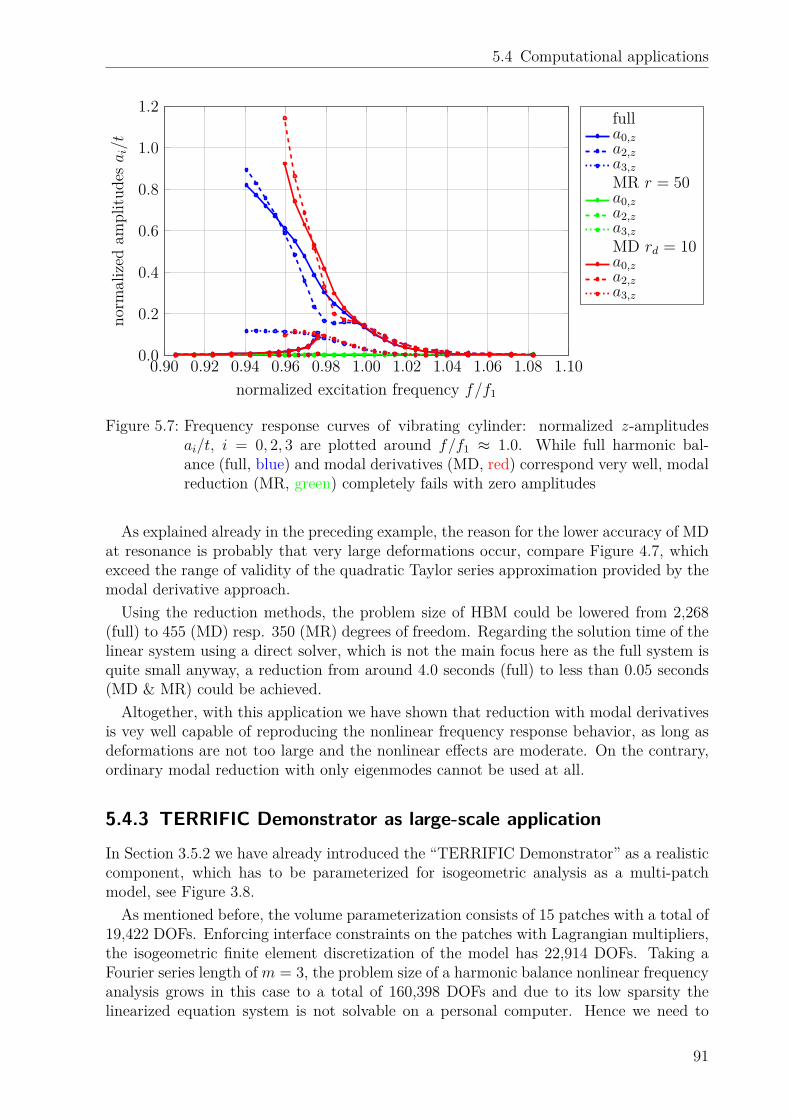
5.4 Computational applications
0.90 0.92 0.94 0.96 0.98 1.00 1.02 1.04 1.06 1.08 1.100.0
0.2
0.4
0.6
0.8
1.0
1.2
normalized excitation frequency f/f1
norm
aliz
edam
plitu
desai/t
fulla0,za2,za3,zMR r = 50a0,za2,za3,zMD rd = 10a0,za2,za3,z
Figure 5.7: Frequency response curves of vibrating cylinder: normalized z-amplitudesai/t, i = 0, 2, 3 are plotted around f/f1 ≈ 1.0. While full harmonic bal-ance (full, blue) and modal derivatives (MD, red) correspond very well, modalreduction (MR, green) completely fails with zero amplitudes
As explained already in the preceding example, the reason for the lower accuracy of MDat resonance is probably that very large deformations occur, compare Figure 4.7, whichexceed the range of validity of the quadratic Taylor series approximation provided by themodal derivative approach.
Using the reduction methods, the problem size of HBM could be lowered from 2,268(full) to 455 (MD) resp. 350 (MR) degrees of freedom. Regarding the solution time of thelinear system using a direct solver, which is not the main focus here as the full system isquite small anyway, a reduction from around 4.0 seconds (full) to less than 0.05 seconds(MD & MR) could be achieved.
Altogether, with this application we have shown that reduction with modal derivativesis vey well capable of reproducing the nonlinear frequency response behavior, as long asdeformations are not too large and the nonlinear effects are moderate. On the contrary,ordinary modal reduction with only eigenmodes cannot be used at all.
5.4.3 TERRIFIC Demonstrator as large-scale application
In Section 3.5.2 we have already introduced the “TERRIFIC Demonstrator” as a realisticcomponent, which has to be parameterized for isogeometric analysis as a multi-patchmodel, see Figure 3.8.
As mentioned before, the volume parameterization consists of 15 patches with a total of19,422 DOFs. Enforcing interface constraints on the patches with Lagrangian multipliers,the isogeometric finite element discretization of the model has 22,914 DOFs. Taking aFourier series length of m = 3, the problem size of a harmonic balance nonlinear frequencyanalysis grows in this case to a total of 160,398 DOFs and due to its low sparsity thelinearized equation system is not solvable on a personal computer. Hence we need to
91
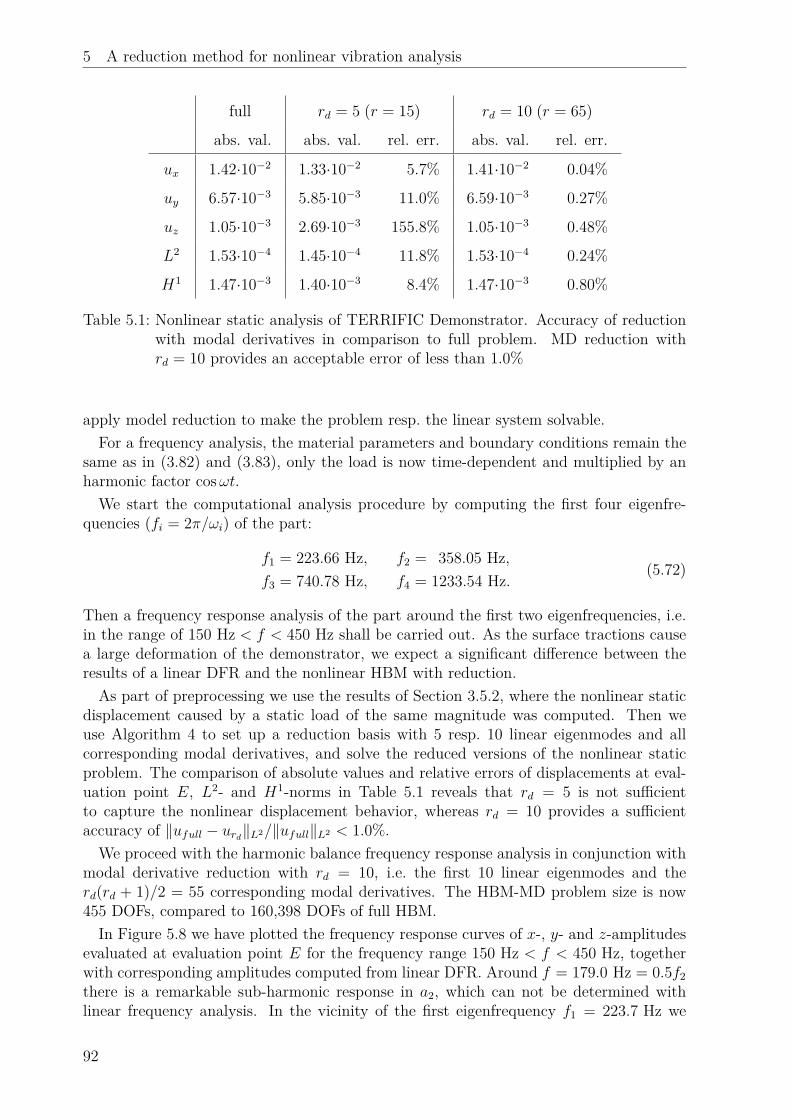
5 A reduction method for nonlinear vibration analysis
full rd = 5 (r = 15) rd = 10 (r = 65)
abs. val. abs. val. rel. err. abs. val. rel. err.
ux 1.42·10−2 1.33·10−2 5.7% 1.41·10−2 0.04%
uy 6.57·10−3 5.85·10−3 11.0% 6.59·10−3 0.27%
uz 1.05·10−3 2.69·10−3 155.8% 1.05·10−3 0.48%
L2 1.53·10−4 1.45·10−4 11.8% 1.53·10−4 0.24%
H1 1.47·10−3 1.40·10−3 8.4% 1.47·10−3 0.80%
Table 5.1: Nonlinear static analysis of TERRIFIC Demonstrator. Accuracy of reductionwith modal derivatives in comparison to full problem. MD reduction withrd = 10 provides an acceptable error of less than 1.0%
apply model reduction to make the problem resp. the linear system solvable.For a frequency analysis, the material parameters and boundary conditions remain the
same as in (3.82) and (3.83), only the load is now time-dependent and multiplied by anharmonic factor cosωt.
We start the computational analysis procedure by computing the first four eigenfre-quencies (fi = 2π/ωi) of the part:
f1 = 223.66 Hz, f2 = 358.05 Hz,f3 = 740.78 Hz, f4 = 1233.54 Hz.
(5.72)
Then a frequency response analysis of the part around the first two eigenfrequencies, i.e.in the range of 150 Hz < f < 450 Hz shall be carried out. As the surface tractions causea large deformation of the demonstrator, we expect a significant difference between theresults of a linear DFR and the nonlinear HBM with reduction.
As part of preprocessing we use the results of Section 3.5.2, where the nonlinear staticdisplacement caused by a static load of the same magnitude was computed. Then weuse Algorithm 4 to set up a reduction basis with 5 resp. 10 linear eigenmodes and allcorresponding modal derivatives, and solve the reduced versions of the nonlinear staticproblem. The comparison of absolute values and relative errors of displacements at eval-uation point E, L2- and H1-norms in Table 5.1 reveals that rd = 5 is not sufficientto capture the nonlinear displacement behavior, whereas rd = 10 provides a sufficientaccuracy of ‖ufull − urd‖L2/‖ufull‖L2 < 1.0%.
We proceed with the harmonic balance frequency response analysis in conjunction withmodal derivative reduction with rd = 10, i.e. the first 10 linear eigenmodes and therd(rd + 1)/2 = 55 corresponding modal derivatives. The HBM-MD problem size is now455 DOFs, compared to 160,398 DOFs of full HBM.
In Figure 5.8 we have plotted the frequency response curves of x-, y- and z-amplitudesevaluated at evaluation point E for the frequency range 150 Hz < f < 450 Hz, togetherwith corresponding amplitudes computed from linear DFR. Around f = 179.0 Hz = 0.5f2there is a remarkable sub-harmonic response in a2, which can not be determined withlinear frequency analysis. In the vicinity of the first eigenfrequency f1 = 223.7 Hz we
92

5.4 Computational applications
150 200 250 300 350 400 450−0.10
−0.05
0.00
0.05
0.10
excitation frequency f [Hz]
ampl
itude
sai,x
[m]
DFRa1,xHBM-MDa0,xa1,xa2,xa3,x
(a) x-amplitudes
150 200 250 300 350 400 450−0.10
−0.05
0.00
0.05
excitation frequency f [Hz]
ampl
itude
sai,y
[m]
DFRa1,yHBM-MDa0,ya1,ya2,ya3,y
(b) y-amplitudes
150 200 250 300 350 400 450−4.00
−2.00
0.00
2.00
·10−2
excitation frequency f [Hz]
ampl
itude
sai,z
[m]
DFRa1,zHBM-MDa0,za1,za2,za3,z
(c) z-amplitudes
Figure 5.8: Frequency response curves of amplitudes of vibrating TERRIFIC Demonstra-tor for DFR (dashed lines) and HBM with MD reduction (solid lines). HBM-MD shows strong nonlinear contributions of higher harmonics at f ≈ 358 Hzand can also detect a sub-harmonic resonance at f ≈ 179 Hz
93

5 A reduction method for nonlinear vibration analysis
Figure 5.9: Snapshots of vibrating TERRIFIC Demonstrator for f = 331.3 Hz at non-dimensional times τ = 0, π/2, π, 3π/2. Significant deviations between non-linear deformation from HBM-MD (colored by von Mises stress in Pa), andlinear DFR deformation (in gray) are visible. Undeformed configuration isalso shown in gray
94

5.4 Computational applications
0 12π
π 32π
2π
−0.10
−0.05
0.00
0.05
0.10
non-dimensional time τ = 2πf t
disp
lace
men
tui
[m]
DFRuxuyuzHBM-MDuxuyuz
Figure 5.10: Displacement of evaluation point on TERRIFIC Demonstrator over one pe-riod of vibration for f = 331.3 Hz for HBM-MD (solid lines) and DFR(dashed lines). Significant deviations due to nonlinear effects are visible
notice that the nonlinear response behavior in z-amplitudes is different from the linearone obtained from DFR, but with our simple frequency stepping method we cannot followcomplex solution paths here. The resonance behavior around f2 = 358.0 Hz is verystrong and we have convergence problems with our method for 335 Hz < f < 355 Hz.There are strong contributions from higher harmonics here, which lead to much morerealistic deformations as we discuss in more detail below. Rapidly growing z-amplitudesat resonance indicate that there might by turning points in the frequency response curveshere, which we could only follow using continuation methods.
Figure 5.9 shows the vibrating structure at a frequency of f = 331.3 Hz, i.e. nearthe first eigenfrequency of f1 = 358.1 Hz, where resonance with very large deformationoccurs. The four snapshots are taken at times τ = 0, π/2, π, 3π/2 display the deformedstructure from the HBM-MD computation colored by von Mises stress in Pa. As referencesthe deformed structure from DFR linear frequency analysis and undeformed structureboth also shown in gray. It is obvious that the nonlinear results lead to a much betterprediction of the small volume change of the structure and thus much more realistic statesof deformation than linear DFR. Furthermore, it is interesting that the bending of thestructure is stronger in the nonlinear case than in the linear case for τ = π.
These findings can also be observed in Figure 5.10, where we have plotted the x-, y-and z-displacement at the evaluation point over one vibration period of τ ∈ [0, 2π] forf = 331.3 Hz for both HBM-MD and DFR. Significant differences are visible between thenonlinear deformation from HBM-MD (solid lines) and the linear deformation from DFR(dashed lines).
Altogether, the results presented here for the “TERRIFIC Demonstrator” show that areduction with modal derivatives makes harmonic balance nonlinear frequency responseanalysis feasible for larger scale applications. Although we do not have the solutionsof a full, unreduced nonlinear frequency analysis here as reference, the results could bevalidated in comparison to linear DFR. It could be shown that HBM-MD is able to capturenonlinear effects such as sub-harmonic resonance and provide much more realistic resultsthan DFR for large amplitude vibrations.
95

5 A reduction method for nonlinear vibration analysis
5.5 Summary
The harmonic balance method, as we have introduced it in Chapter 4, is a powerful meansfor nonlinear steady-state frequency analysis. However, its major drawback is the size ofthe resulting linear system to be solved, which makes HBM unfeasible for large problems.In this chapter we have addressed this issue and proposed a model order reduction methodfor the spatial discretization, which reduces the problem size significantly and enableslarge-scale applications.
After a review of commonly used projection methods for model order reduction, we havedecided to use a modal projection basis, which is enhanced with modal derivatives (MD).We have introduced the concept of modal derivatives and shown that modal derivativescan be used to obtain a second-order approximation of displacements. This motivatedthe use of MD for model reduction in nonlinear frequency analysis and HBM.
In order to gain a better understanding of the concept, we have established a moretheoretical framework by transferring the idea of modal derivatives to the continuousformulation of PDE problems. Using a model problem and the nonlinear Euler-Bernoullibeam as examples, we could show that MDs can be analytically computed and used toapproximate the exact solutions.
With computational examples we could demonstrate that reduction with modal deriva-tives is very accurate for moderate nonlinearities. Also the application in nonlinear fre-quency response analysis was successful and HBM-MD could approximate the results offull HBM very well. It provides a substantial reduction of the total number of DOFs,but is at the same time still able to reproduce the main characteristics of nonlinear vi-brations, such as sub-harmonic resonances. With the TERRIFIC Demonstrator we haveshown that a larger scale nonlinear frequency analysis is now feasible with HBM-MD.
96
6 Isogeometric mixed methods fornear incompressible vibrations
An important practical application of the method for nonlinear vibration analysis usingisogeometric finite elements, harmonic balance, and modal derivative reduction, which wehave developed over the preceding chapters, is the simulation of rubber and elastomercomponents. These are described using incompressible and near incompressible visco-hyperelastic materials laws, which have a Poisson’s ratio ν equal or very close to 0.5. Inthis situation, finite element methods used without particular care can lead to lockingphenomena, and consequently unreliable numerical simulations [23].
In the following we discuss the phenomenon of volumetric locking and review possi-ble cures in Section 6.1. To avoid locking in near incompressible elasticity, we presentisogeometric mixed finite element methods in Section 6.2. We integrate these mixed meth-ods also into our framework for nonlinear frequency analysis, i.e. the harmonic balancemethod, in Section 6.3 and study their performance for application in nonlinear staticand frequency response analysis numerically in Section 6.4.
6.1 Near incompressibility and locking
Locking phenomena can be observed for all kinds of physical problems subject to con-straints, such as fluid mechanics with incompressible Stokes and Navier-Stokes equations,continuum mechanics with near incompressible elasticity and plasticity (volumetric lock-ing), and structural elements such as thin plates, shells and beams (shear and membranelocking) [23, 130]. The term locking means that a finite element formulation underes-timates the true or analytical solution of a problem, i.e. it shows an unphysically stiffbehavior and only converges very slowly, as can be seen in later presented numericalexamples in Section 6.4.
In elasticity, the constitutive equation dependends on the two parameters µ and λ, theso-called Lame constants, compare Section 3.1.3. When Poisson’s ratio ν → 0.5, it followsthat
µ→ E
3 , λ→∞, (6.1)
which leads for near incompressible problems to an ill-conditioning of the stiffness matrixand thus volumetric locking, and for full incompressiblity conventional methods cannotbe used at all.
97

6 Isogeometric mixed methods for near incompressible vibrations
The incompressibility condition, which is div u = 0 in linear and J = 1 in nonlinearelasticity, acts as an additional constraint for the deformation control points or nodes.For example, a linear triangular finite element can completely lock in incompressible 2Dplain strain problems and allows no deformation at all for a whole mesh [39].
For higher-order finite elements, such as p-FEM and isogeometric methods, volumetriclocking effects are alleviated or even totally disappearing for very high degree p. However,it is not always desireable to use very high orders due to limited regularity of the exactsolution and lower sparsity of resulting stiffness matrices [130], which applies for bothp-FEM and IGA.
A number of alternative methods have been developed for locking-free finite element dis-cretizations and many of them have been adapted to the context of isogeometric analysisalready: Mixed formulations for the incompressible Stokes problem in 2D where inves-tigated in [30] and mixed three-field formulations based on the Hu-Washizu functionalfor (near) incompressible linear and nonlinear elasticity and plasticity in [84, 118]. Astream function formulation, where the divergence-free constraint is directly imposed onthe discretization space, was studied for plain elasticity problems in [4]. The same class ofproblems was treated by B- and F -projection methods in [48]. Furthermore, the assumednatural strain (ANS) method for shells [32] and descrete shear gap (DSG) and reducedintegration methods for Timoshenko beams [24, 47] were investigated.
6.2 Isogeometric mixed finite element discretizations
In order to cure volumetric locking and be able to accurately solve near and fully incom-pressible elasticity problems, we employ a mixed method. In a mixed method applied toa certain formulation, such as the elasticity equations, different variables are discretizedindependently from each other. In [33] we have already described the isogeometric finiteelement discretization of mixed formulations and their implementation using igatoolssoftware library [91]. Here we review the derivation of mixed formulations for near andfully incompressible, linear and nonlinear elasticity based on references [6, 7, 23, 109, 130],and outline the discretization using different kinds of mixed isogeometric elements.
6.2.1 Formulation for linear (near) incompressibility
To describe the mixed methods, we begin with the static linear elasticity equation and thecorresponding energy functional, which was already introduced in Section 3.3 as (3.62),and is only displacement-based:
ψd(u) = µ tr(ε2(u)) + λ
2 tr(ε(u))2. (6.2)
Now we introduce the pressure-like scalar variable p = λ tr(ε(u)) and rewrite the strainenergy functional in a mixed form depending on both u and p [6]:
ψm(u, p) = µ tr(ε2(u)) + p tr(ε(u))− 12λ p
2. (6.3)
98
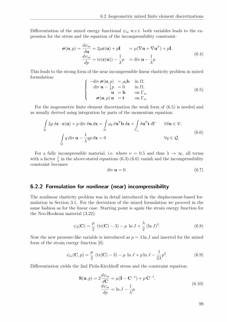
6.2 Isogeometric mixed finite element discretizations
Differentiation of the mixed energy functional ψm w.r.t. both variables leads to the ex-pression for the stress and the equation of the incompressibility constraint:
σ(u, p) = dψmdu
= 2µε(u) + pI = µ(∇u +∇uT ) + pI,
dψmdp
= tr(ε(u))− 1λp = div u− 1
λp
(6.4)
This leads to the strong form of the near incompressible linear elasticity problem in mixedformulation:
−div σ(u, p) = ρ0b in Ω,div u− 1
λp = 0 in Ω,u = h on Γu,
σ(u, p) n = t on Γn.
(6.5)
For the isogeometric finite element discretization the weak form of (6.5) is needed andas usually derived using integration by parts of the momentum equation:∫
Ω
2µ δε · ε(u) + p div δu dx =∫Ω
ρ0 δuTb dx +∫
Γn
δuT t dΓ ∀δu ∈ V ,
∫Ω
q div u− 1λqp dx = 0 ∀q ∈ Q.
(6.6)
For a fully incompressible material, i.e. where ν = 0.5 and thus λ → ∞, all termswith a factor 1
λin the above-stated equations (6.3)-(6.6) vanish and the incompressibility
constraint becomesdiv u = 0. (6.7)
6.2.2 Formulation for nonlinear (near) incompressibility
The nonlinear elasticity problem was in detail introduced in the displacement-based for-mulation in Section 3.1. For the derivation of the mixed formulation we proceed in thesame fashion as for the linear case. Starting point is again the strain energy function forthe Neo-Hookean material (3.22):
ψd(C) = µ
2 (tr(C)− 3)− µ ln J + λ
2 (ln J)2. (6.8)
Now the new pressure-like variable is introduced as p = λ ln J and inserted for the mixedform of the strain energy function [6]:
ψm(C, p) = µ
2 (tr(C)− 3)− µ ln J + p ln J − 12λp
2. (6.9)
Differentiation yields the 2nd Piola-Kirchhoff stress and the constraint equation:
S(u, p) = 2dψmdC
= µ(I−C−1) + pC−1,
dψmdp
= ln J − 1λp.
(6.10)
99

6 Isogeometric mixed methods for near incompressible vibrations
It follows the strong form of the near incompressible nonlinear hyperelasticity problem inmixed formulation:
−div (F S(u, p)) = ρ0b in Ω,ln J − 1
λp = 0 in Ω,u = h on Γu,
F S(u, p) n = t on Γn.
(6.11)
As in Section 3.2.1, the weak form of (6.11) is be derived before a mixed finite elementdiscretization can be applied:∫
Ω
δE · S(u, p) dx =∫Ω
ρ0δuTb dx +∫
Γn
δuTg dΓ ∀δu ∈ V ,
∫Ω
q ln J − 1λqp dx = 0 ∀q ∈ Q.
(6.12)
In the case of a fully incompressible material with λ→∞, again all terms with a factor1λ
vanish and the incompressibility constraint becomes
ln J = 0, (6.13)
which is equal to the earlier mentioned constrained J = det F = 1. Depending on the non-linear material law, different incompressibility constraints may be chosen as alternativesto (6.13). Commonly used are also J2 − 1, J − 1 and 1− 1/J [7, 130].
6.2.3 Mixed isogeometric elements
Having derived the weak forms of the (near) incompressible elasticity problem in the linearand nonlinear setting as mixed formulations with (6.6) and (6.12), the next step in thesolution of these equations is the discretization of spaces V ⊂ H1(Ω)3 and Q ⊂ L2(Ω). Inour setting we certainly choose the discrete spaces Vh ⊂ V and Qh ⊂ Q as (refinementsof) the push-forward of spline function spaces on the domain Ω.
For the linear problem, this results in a symmetric, block-structured system of equationsof size Nu +Np: (
K BT
B Q
)(dλ
)=(
b0
), (6.14)
with d ∈ RNu and λ ∈ RNp .In the incompressible case the matrix Q is zero and in the near-incompressible it is
almost zero due to the factor 1λ. The pressure like variable p, which is discretized using
the coefficient vector λ, acts as a Lagrangian multiplier for the incompressibility constraintand this means that (6.14) is a (perturbed) saddle point problem. In Section 2.3.3 wehave already encountered saddle point problems arising from multi-patch discretizationsand seen that the rank of the sub-matrix B is crucial for the solvability of the system.
In the context of a mixed discretization, B arises from the assembly of the term b(v, q) =∫Ω q div v dx, where both discretization spaces are mixed since vh ∈ Vh and qh ∈ Qh. The
full-rank condition for B then leads to the well-known Babuska-Brezzi or inf-sup condition
100

6.2 Isogeometric mixed finite element discretizations
for Vh and Qh [7, 23, 35]:
infq∈Qh,q 6=0
supv∈Vh,v 6=0
b(v, q)‖q‖L2‖v‖H1
≥ ε > 0. (6.15)
Furthermore, as for the displacement-based case, the following coercivity condition musthold for the bilinear form a(v,u) =
∫Ω 2µ ε(v) · ε(u) dx [7, 23, 35]:
infv∈Vh,v6=0,div v=0
a(v,v)‖v‖2
H1≥ ε > 0. (6.16)
Thus the choice of a combination of spaces for the discretization of displacement andpressure, i.e. the choice of a mixed element Vh/Qh, is crucial for the stability of the method[7]. For the linear Stokes problem a mathematical analysis of mixed isogeometric finiteelement types based on NURBS discretizations has been carried out in [28], and the twoproposed inf-sup-stable element types are presented in the following.
In the nonlinear case, the discretization of (6.12) leads to a nonlinear system of theform (
f(d,λ)c(d,λ)
)=(
b0
). (6.17)
For an iterative solution of this nonlinear system of equations, compare the Newton’smethod for the displacement-based formulation presented in Algorithm 1, the linearizationof (6.17) is needed and leads to a linear system with the very same block structure as(6.14).
Taylor-Hood elements
Taylor-Hood elements (TH) are well-established in classical finite element analysis andtheir isogeometric counterparts have already been employed in [14] for incompressibleelasticity. Isogeometric TH elements are denoted by Srp+1/Srp and based on the samemesh Th(Ω) for the discretization of displacements and pressure, but the degree of Vh isone higher than of Qh:
Qh = Srp(Th(Ω)
), Vh =
(Srp+1
(Th(Ω)
))d. (6.18)
This means that Vh is obtained from Qh by one step of p-refinement, i.e. an order elevationthat maintains the regularity r < p of the pressure space also for the displacement space.In [28] it is proven that the isogeometric Taylor-Hood elements Srp+1/Srp are inf-sup stablefor p ≥ 1.
As introduced before in Section 2.1, the notation Srp(Th(Ω)
)refers to a tensor product
spline space, which is defined as push-forward of spline functions on the physical domainΩ, based on the mesh Th(Ω).
Example 6.1 (Isogeometric Taylor-Hood element S13/S1
2 ). Figure 6.1 shows the B-Splinebasis functions of a one-dimensional isogeometric Taylor-Hood element S1
3/S12 with the
101
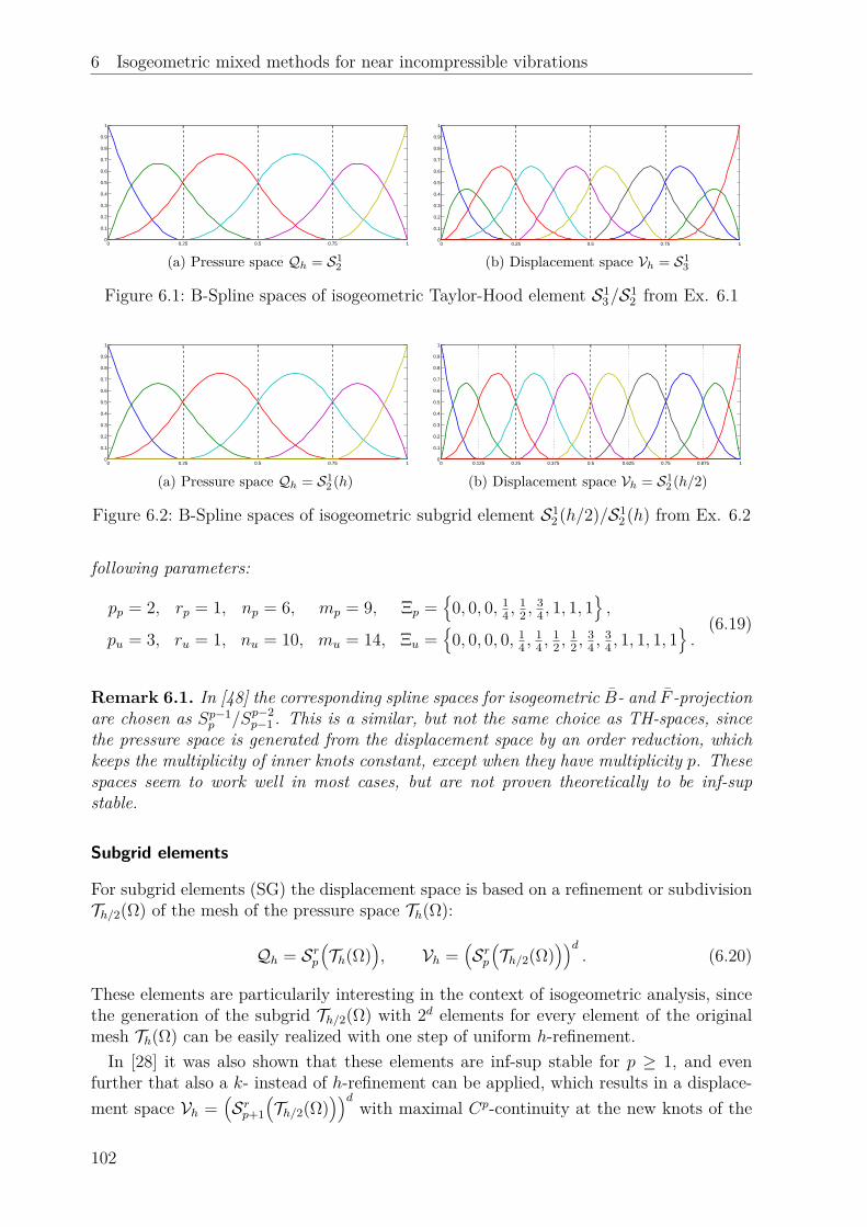
6 Isogeometric mixed methods for near incompressible vibrations
0 0.25 0.5 0.75 10
0.1
0.2
0.3
0.4
0.5
0.6
0.7
0.8
0.9
1
(a) Pressure space Qh = S12
0 0.25 0.5 0.75 10
0.1
0.2
0.3
0.4
0.5
0.6
0.7
0.8
0.9
1
(b) Displacement space Vh = S13
Figure 6.1: B-Spline spaces of isogeometric Taylor-Hood element S13/S1
2 from Ex. 6.1
0 0.25 0.5 0.75 10
0.1
0.2
0.3
0.4
0.5
0.6
0.7
0.8
0.9
1
(a) Pressure space Qh = S12 (h)
0 0.125 0.25 0.375 0.5 0.625 0.75 0.875 10
0.1
0.2
0.3
0.4
0.5
0.6
0.7
0.8
0.9
1
(b) Displacement space Vh = S12 (h/2)
Figure 6.2: B-Spline spaces of isogeometric subgrid element S12 (h/2)/S1
2 (h) from Ex. 6.2
following parameters:
pp = 2, rp = 1, np = 6, mp = 9, Ξp =
0, 0, 0, 14 ,
12 ,
34 , 1, 1, 1
,
pu = 3, ru = 1, nu = 10, mu = 14, Ξu =
0, 0, 0, 0, 14 ,
14 ,
12 ,
12 ,
34 ,
34 , 1, 1, 1, 1
.
(6.19)
Remark 6.1. In [48] the corresponding spline spaces for isogeometric B- and F -projectionare chosen as Sp−1
p /Sp−2p−1 . This is a similar, but not the same choice as TH-spaces, since
the pressure space is generated from the displacement space by an order reduction, whichkeeps the multiplicity of inner knots constant, except when they have multiplicity p. Thesespaces seem to work well in most cases, but are not proven theoretically to be inf-supstable.
Subgrid elements
For subgrid elements (SG) the displacement space is based on a refinement or subdivisionTh/2(Ω) of the mesh of the pressure space Th(Ω):
Qh = Srp(Th(Ω)
), Vh =
(Srp(Th/2(Ω)
))d. (6.20)
These elements are particularily interesting in the context of isogeometric analysis, sincethe generation of the subgrid Th/2(Ω) with 2d elements for every element of the originalmesh Th(Ω) can be easily realized with one step of uniform h-refinement.
In [28] it was also shown that these elements are inf-sup stable for p ≥ 1, and evenfurther that also a k- instead of h-refinement can be applied, which results in a displace-ment space Vh =
(Srp+1
(Th/2(Ω)
))dwith maximal Cp-continuity at the new knots of the
102
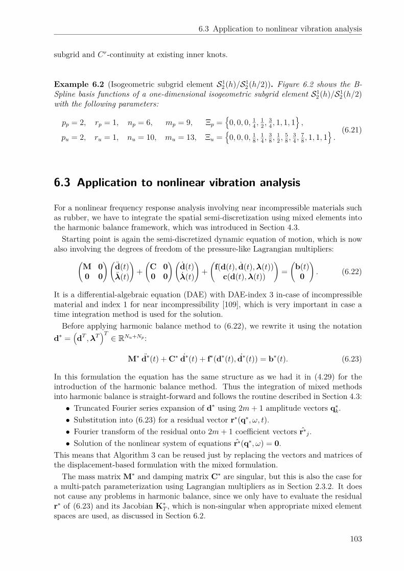
6.3 Application to nonlinear vibration analysis
subgrid and Cr-continuity at existing inner knots.
Example 6.2 (Isogeometric subgrid element S12 (h)/S1
2 (h/2)). Figure 6.2 shows the B-Spline basis functions of a one-dimensional isogeometric subgrid element S1
2 (h)/S12 (h/2)
with the following parameters:
pp = 2, rp = 1, np = 6, mp = 9, Ξp =
0, 0, 0, 14 ,
12 ,
34 , 1, 1, 1
,
pu = 2, ru = 1, nu = 10, mu = 13, Ξu =
0, 0, 0, 18 ,
14 ,
38 ,
12 ,
58 ,
34 ,
78 , 1, 1, 1
.
(6.21)
6.3 Application to nonlinear vibration analysis
For a nonlinear frequency response analysis involving near incompressible materials suchas rubber, we have to integrate the spatial semi-discretization using mixed elements intothe harmonic balance framework, which was introduced in Section 4.3.
Starting point is again the semi-discretized dynamic equation of motion, which is nowalso involving the degrees of freedom of the pressure-like Lagrangian multipliers:(
M 00 0
)(d(t)λ(t)
)+(
C 00 0
)(d(t)λ(t)
)+(
f(d(t), d(t),λ(t))c(d(t),λ(t))
)=(
b(t)0
). (6.22)
It is a differential-algebraic equation (DAE) with DAE-index 3 in-case of incompressiblematerial and index 1 for near incompressibility [109], which is very important in case atime integration method is used for the solution.
Before applying harmonic balance method to (6.22), we rewrite it using the notationd∗ =
(dT ,λT
)T∈ RNu+Np :
M∗ d∗(t) + C∗ d∗(t) + f∗(d∗(t), d∗(t)) = b∗(t). (6.23)
In this formulation the equation has the same structure as we had it in (4.29) for theintroduction of the harmonic balance method. Thus the integration of mixed methodsinto harmonic balance is straight-forward and follows the routine described in Section 4.3:• Truncated Fourier series expansion of d∗ using 2m+ 1 amplitude vectors q∗k.• Substitution into (6.23) for a residual vector r∗(q∗, ω, t).• Fourier transform of the residual onto 2m+ 1 coefficient vectors r∗j.• Solution of the nonlinear system of equations r∗(q∗, ω) = 0.
This means that Algorithm 3 can be reused just by replacing the vectors and matrices ofthe displacement-based formulation with the mixed formulation.
The mass matrix M∗ and damping matrix C∗ are singular, but this is also the case fora multi-patch parameterization using Lagrangian multipliers as in Section 2.3.2. It doesnot cause any problems in harmonic balance, since we only have to evaluate the residualr∗ of (6.23) and its Jacobian K∗T , which is non-singular when appropriate mixed elementspaces are used, as discussed in Section 6.2.
103

6 Isogeometric mixed methods for near incompressible vibrations
Near incompressible, visco-hyperelastic materials
In (6.22) we have stated that the internal force vector f(d(t), d(t),λ(t)) may also dependon the velocities, as it is the case for visco-hyperelastic materials (Section 3.1.4), but sofar in the derivation of nonlinear near incompressible elasticity in Section 6.2.2 this wasn’tconsidered yet.
Hence we now introduce a near incompressible, visco-hyperelastic constitutive rela-tion by augmenting the 2nd Piola-Kirchhoff stress term of the near incompressible Neo-Hookean material model from (6.10) with the viscous stress term from (3.31):
S(u, u, p) = Se(u, p) + Sv(u, u) = µ(I−C−1) + pC−1 + 2ηµE. (6.24)
6.4 Computational applications
In the following computational examples we want to study the performance of differentisogeometric mixed finite element formulations, i.e. Taylor-Hood and subgrid elements,in application to nonlinear near incompressible elasticity and compare the to purely dis-placement based formulations. Furthermore, the use of mixed formulations within thenonlinear frequency response analysis framework is investigated.
6.4.1 Cook’s membrane as benchmark problem
A popular test problem for validation and benchmarking of locking-free finite elementdiscretizations is Cook’s membrane problem [38]. It has also been used in the context ofisogeometric methods [48, 84], and we have employed it in [33] to validate our implemen-tation using igatools library [91].
Cook’s membrane is a 2D panel, clamped on the left side and subject to a shear load onthe right side, causing combined bending and shear deformation. Geometry, dimensionsand values of parameters can be found in Figure 6.3(a). Large deformation kinematicsand the nonlinear, near incompressible Neo-Hookean constitutive law are employed. Thequantity of interest is the horizontal deformation of the top right corner of the paneluy, which is used to study p/k- and h-convergence and locking-free behavior of mixedelements. An example for a large deformation of the panel is visualized in Figure 6.3(b).
First, the convergence behavior of isogeometric finite element formulations is studiedfor near incompressibility with ν → 0.5 and summarized in Table 6.1 and Figure 6.4. Themixed Taylor-Hood element S1
3(h)/S12(h) and mixed subgrid element S1
2(h/2)/S12(h) are
compared to the displacement-based element S23(h) for ν being increased from 0.4 to 0.5.
For increasing incompressibility, i.e. ν → 0.5 and λ/µ = 2ν1−2ν →∞, it can be seen that
the accuracy of the displacement-based element S23 decreases due to volumetric locking,
while the mixed methods converge. Furthermore, for the mixed elements the numberof iterations for convergence of the Newton’s method is independent of ν, while it in-creases also for the non-mixed element and even load-stepping has to be applied to ensureconvergence in the very near incompressible regime, which is another indicator of locking.
In Figure 6.5 convergence behavior of uy with respect to the number of elements perside (` ∼ 1/h) of the discretization of the panel is shown. We compare the isogeomet-ric Taylor-Hood and subgrid elements with pure displacement formulations for a fixed
104

6.4 Computational applications
x
y
48 mm
44 mm
16 mm F
uy
E = 240.565 MPaνd = 0.499νm = 0.5F = 100 kN
(a) Geometry and parameters of Cook’s membraneproblem
(b) Deformed Cook’s membrane colored bypressure in Pa
Figure 6.3: Problem setting of Cook’s membrane and deformation plot
TH S13/S
12 SG S1
2/S12 displ. S2
3
ν λ/µ uy it. uy it. uy it.0.4 4 7.4045 5 7.3955 5 7.3324 50.45 9 7.1660 5 7.1551 5 7.0572 60.49 49 6.9393 5 6.9262 5 6.7398 90.495 99 6.9085 5 6.8951 5 6.6627 80.499 499 6.8834 5 6.8698 5 6.5089 80.4999 4999 6.8778 5 6.8640 5 6.3179 2 · 80.49999 49999 6.8772 5 6.8635 5 6.0424 4 · 90.499999 499999 6.8771 5 6.8634 5 5.7274 10 · 8
Table 6.1: Convergence study of Cook’s membrane for near incompressibility with Pois-son’s ratio ν → 0.5, comparison of uy in mm and number of Newton iterations
Poisson’s ratio ν = 0.499. The classical displacement-based Sp−1p elements show a rather
slow convergence behavior due to locking, while both mixed elements, Taylor-Hood andsubgrid, converge quickly for p/k- and h-refinement. These results also match very wellwith the ones obtained by [48], where an isogeometric F -method was used instead of amixed formulation. The accuracy of Taylor-Hood elements Sp−1
p+1(h)/Sp−1p (h) is a bit higher
than of subgrid elements Sp−1p (h/2)/Sp−1
p (h). For same degree p both elements have thesame number of degrees of freedom, since the increase in DOFs is the same for p- andh-refinement, but the benefit of a higher degree is larger than the one of a finer mesh.
Even though the purely displacement formulation also converges toward the correctvalue of uy for higher polynomial degree and number of degrees of freedom, the approxi-mation of stresses exhibits spurious oscillations, which are typical for locking phenomena.In Figure 6.6 we plot the stress component σxx. The non-mixed elements show a highlyoscillatory behavior of volumetric stress components – a typical sign of volumetric locking
105

6 Isogeometric mixed methods for near incompressible vibrations
100 101 102 103 104 105 1065.5
6.0
6.5
7.0
7.5
incompressibility ratio λ/µ
y-di
spla
cem
entuy
[mm
] displ. S23
TH S13/S
12
SG S12/S
12
Figure 6.4: Convergence of displacement uy of Cook’s membrane over incompressibilityratio λ/µ for near incompressibility as Poisson’s ratio ν → 0.5
1 2 4 8 16 320.0
2.0
4.0
6.0
8.0
elements per side `
y-di
spla
cem
entuy
[mm
] displ. S01
displ. S12
displ. S23
TH S02/S
01
TH S13/S
12
SG S01/S
01
SG S12/S
12
Figure 6.5: p/h/k-convergence of y-displacement uy of Cook’s membrane over number ofelements per side ` for displacement-based and mixed formulations
– while the stress distributions for mixed Taylor-Hood elements are smooth.Altogether, we have demonstrated the signs of locking of purely-displacement based
elements in the near incompressible regime, which are a deterioration of convergence andstress oscillations, and we have seen numerically that mixed methods can resolve thisproblem.
6.4.2 Nonlinear vibration of a thick rubber cylinder
Having studied the convergence of mixed elements, we now want to move to nonlinearvibration analysis. As an application we choose a thick rubber cylinder with the samegeometry, dimensions and symmetry boundary conditions as the one used in Section 3.5.1,Figure 3.6(a).
106

6.4 Computational applications
(a) S23 with 4 elements per side (b) S1
3/S12 with 4 elements per side
(c) S23 with 16 elements per side (d) S1
3/S12 with 16 elements per side
Figure 6.6: Comparison of stress component σxx for displacement-based S23 and mixed
S13/S
12 Taylor-Hood element for 4 (top) resp. 16 (bottom) elements per side at
ν = 0.499. Displacement-based elements exhibit strong oscillations of stresses
Convergence for static displacement and eigenfrequencies
First we want to check the accuracy and convergence of the mixed and displacement-based formulations and elements for static nonlinear deformation and eigenfrequencies.The results are summarized in Figure 6.7. S1
2 and S23 refer to displacement-based elements,
with p = 2, 3 in all three parameter directions, h-refined such that at maximal mesh sizeparameter h was obtained, and C1- resp. C2-continuous at inner knots, since the originalgeometry did not contain any inner knots. S0
2/S01 and S1
3/S12 refer to mixed Taylor-
Hood elements, where the displacement space is obtained from the pressure space byp-refinement, with preceding h-refinement to obtain maximal mesh size parameter h. Asummary of number of degrees of freedom for these discretizations is given in Table 6.2.
For static nonlinear deformation we assume a vertically directed surface load (Neumannboundary condition) on the outer shell of the cylinder with magnitude −3.0 kN, a constant
107

6 Isogeometric mixed methods for near incompressible vibrations
hS1
2 S23 S0
2/S01 S1
3/S12
nu N nu N nu np N nu np N
0.08 48 144 100 300 48 18 162 144 48 4800.04 108 324 196 588 108 50 374 400 108 13080.02 300 900 484 1452 300 162 1062 1296 300 41880.01 1296 3888 1805 5415 1296 867 4755 6936 1296 22104
Table 6.2: Number of control points and degrees of freedom of spline spaces for mixed anddisplacement-based elements for thick rubber cylinder
Young’s modulus E = 2.432 MPa and constant, nearly incompressible Poisson’s ratioν = 0.495. The mass density of the rubber material is ρ = 1905.7 kg/m3.
Figure 6.7(a) shows the z-displacement at evaluation point E2 and Figure 6.7(b) theL2-norm of displacements for h/k-refinement. With uz = −1.78 cm, the magnitude of thedisplacement is about the thickness of the cylinder, which is t = 2.0 cm. We can observea very slow convergence of S1
2 and a faster convergence of other elements, which is inaccordance with previous results. Especially the mixed element S1
3/S12 is very accurate
already for the coarsest mesh.The performance of mixed and displacement-based elements exhibits also a huge differ-
ence regarding the convergence behavior of the Newton’s method, see Algorithm 1. Fordisplacement-based elements we have to apply load stepping, otherwise the tangent stiff-ness matrix might become singular within the initial few steps of the Newton algorithm.This behavior seems to become worse with increasing degree p and smaller h, and makesthe Sp-elements unreliable. For mixed elements we do not observe any convergence issues.
Furthermore, we also examine the first eigenfrequency f1 and its frequency-dependentcounterpart f1(f), which is obtained using frequency-dependent Young’s modulus E(f)and constant ν = 0.495. The results in Figure 6.8 reveal a very similar convergencebehavior as for the static nonlinear displacement. The values converge to f1 = 10.79 Hzand f1(f) = 20.85 Hz.
Nonlinear frequency response
Now we can compare the mixed and displacement-based elements in a nonlinear fre-quency response analysis with harmonic balance method. We use a visco-hyperelasticNeo-Hookean material and consider the full frequency-dependency of E(f), ν(f) and alsothe loss factor η(f), see Figure 3.3.
We compute the response amplitudes within the range 10.0 Hz ≤ f ≤ 30.0 Hz, i.e.around the first frequency-dependent eigenfrequency f1(f). The magnitude of the surfaceload is increased on −10.0 kN, since E(f) ≈ 3E(0) in the frequency range of interest, andthe load is now harmonic in time with a factor cosωt.
For the isogeometric discretization we use the elements S23 and S1
3/S12 for h = 0.08,
which was the coarsest mesh of our preceding convergence analysis, but already lead tosufficiently accurate results, especially for the mixed method. In the Fourier series ansatzof harmonic balance we include the first two harmonics, i.e. m = 2.
108

6.4 Computational applications
0.01 0.02 0.04 0.08−2.0
−1.5
−1.0
−0.5
0.0·10−2
mesh size parameter h [m]
disp
lace
men
tuz
[m]
S12S2
3S0
2/S01
S13/S
12
(a) z-displacement at evaluation point
0.01 0.02 0.04 0.080.0
0.5
1.0
1.5
2.0
2.5
3.0·10−4
mesh size parameter h [m]
disp
lace
men
tno
rm‖u‖ L
2
S12S2
3S0
2/S01
S13/S
12
(b) L2-norm of displacement
Figure 6.7: Convergence of nonlinear displacement for mixed Sp−1p+1/S
p−1p - and displace-
ment-based Sp−1p -elements for thick rubber cylinder
0.01 0.02 0.04 0.080
10
20
30
40
mesh size parameter h [m]
eige
nfre
quen
ciesf 1
andf 1
(f)
[Hz] f1
S12S2
3S0
2/S01
S13/S
12
f1(f)S1
2S2
3S0
2/S01
S13/S
12
Figure 6.8: Convergence of first eigenfrequency f1 and freq.-dept. eigenfrequency f1(f)for mixed and displacement-based elements for thick rubber cylinder
109
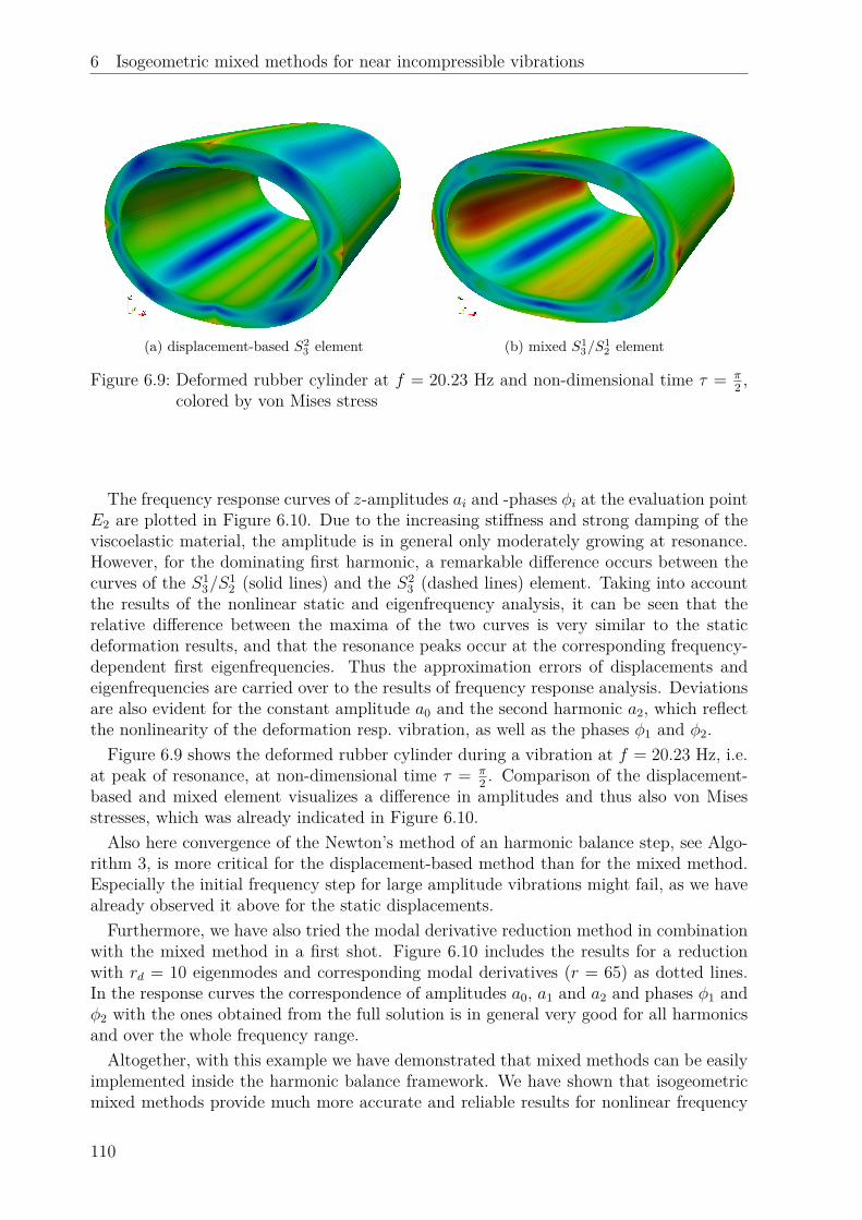
6 Isogeometric mixed methods for near incompressible vibrations
(a) displacement-based S23 element (b) mixed S1
3/S12 element
Figure 6.9: Deformed rubber cylinder at f = 20.23 Hz and non-dimensional time τ = π2 ,
colored by von Mises stress
The frequency response curves of z-amplitudes ai and -phases φi at the evaluation pointE2 are plotted in Figure 6.10. Due to the increasing stiffness and strong damping of theviscoelastic material, the amplitude is in general only moderately growing at resonance.However, for the dominating first harmonic, a remarkable difference occurs between thecurves of the S1
3/S12 (solid lines) and the S2
3 (dashed lines) element. Taking into accountthe results of the nonlinear static and eigenfrequency analysis, it can be seen that therelative difference between the maxima of the two curves is very similar to the staticdeformation results, and that the resonance peaks occur at the corresponding frequency-dependent first eigenfrequencies. Thus the approximation errors of displacements andeigenfrequencies are carried over to the results of frequency response analysis. Deviationsare also evident for the constant amplitude a0 and the second harmonic a2, which reflectthe nonlinearity of the deformation resp. vibration, as well as the phases φ1 and φ2.
Figure 6.9 shows the deformed rubber cylinder during a vibration at f = 20.23 Hz, i.e.at peak of resonance, at non-dimensional time τ = π
2 . Comparison of the displacement-based and mixed element visualizes a difference in amplitudes and thus also von Misesstresses, which was already indicated in Figure 6.10.
Also here convergence of the Newton’s method of an harmonic balance step, see Algo-rithm 3, is more critical for the displacement-based method than for the mixed method.Especially the initial frequency step for large amplitude vibrations might fail, as we havealready observed it above for the static displacements.
Furthermore, we have also tried the modal derivative reduction method in combinationwith the mixed method in a first shot. Figure 6.10 includes the results for a reductionwith rd = 10 eigenmodes and corresponding modal derivatives (r = 65) as dotted lines.In the response curves the correspondence of amplitudes a0, a1 and a2 and phases φ1 andφ2 with the ones obtained from the full solution is in general very good for all harmonicsand over the whole frequency range.
Altogether, with this example we have demonstrated that mixed methods can be easilyimplemented inside the harmonic balance framework. We have shown that isogeometricmixed methods provide much more accurate and reliable results for nonlinear frequency
110

6.4 Computational applications
10 12 14 16 18 20 22 24 26 28 300.0
0.5
1.0
1.5
2.0
2.5·10−2
excitation frequency f [Hz]
ampl
itude
sai
[m]
S23a0a1a2S1
3/S12
a0a1a2S1
3/S12 (MD)
a0a1a2
(a) Amplitudes ai over excitation frequency f
10 12 14 16 18 20 22 24 26 28 30−1.0
−0.8
−0.6
−0.4
−0.20.0
0.2
0.4
0.6
0.8
1.0
excitation frequency f [Hz]
phas
esφi/π
S23φ1φ2S1
3/S12
φ1φ2S1
3/S12 (MD)
φ1φ2
(b) Phases φi over excitation frequency f
Figure 6.10: Nonlinear frequency response curves for thick rubber cylinder. Amplitudesand phases of harmonics at evaluation point for displacement-based S2
3 -element (dashed), mixed S1
3/S12 -formulation (solid line), and mixed formula-
tion with reduction with rd = 10, r = 65 (MD, dotted line)
response analysis with nearly incompressible materials than displacement-based methods.Reduction with modal derivatives seems to work well in the setting of mixed elements andvisco-hyperelasticity, too, but as amplitudes are still moderate here due to damping effects,this has to be investigated in more detail in the future.
111

6 Isogeometric mixed methods for near incompressible vibrations
6.5 Summary
Rubber components are an important application of the nonlinear frequency analysismethod developed over preceding chapters, as they can undergo large amplitude vibra-tions.
However, rubber is a nearly incompressible material and to avoid inaccuracy of numer-ical simulations the phenomenon of volumetric locking has to be considered. Thus wehave first described and explained volumetric locking and reviewed possible cures.
In the context of isogeometric analysis, mixed finite element methods are an auspi-cious method for preventing locking in both linear and nonlinear near incompressibleelasticity. We have outlined the use of two particular isogeometric mixed element types,namely Taylor-Hood and subgrid elements. Both are based on a two-field approach withindependent discretizations of displacement field and a pressure-like variable.
Then we have presented the successful integration of these mixed formulations for nearincompressible, visco-hyperelastic materials into HBM.
Using computational examples, we could demonstrate that Taylor-Hood and subgridelements both perform well also in the nonlinear near incompressible regime. In contrastto purely displacement-based formulations, they prevent locking and exhibit a fast con-vergence behavior without stress oscillations. We could also confirm that the advantagesof mixed methods carry over to nonlinear vibration analysis, where frequency responsecurves are captured much more accurately using the mixed methods. Finally, we havealso tested the modal derivative reduction method and it indicated to be very accuratealso for near incompressible applications.
112

7 Conclusion
7.1 Summary
In this thesis we have developed a novel method for the computational analysis of nonlin-ear steady-state frequency response, which is capable of simulating vibrational behaviorof large-scale applications in solid mechanics. It is mainly based on three pillars: a spa-tial semi-discretization of the nonlinear elastodynamic partial differential equation usingisogeometric finite elements; model order reduction of the resulting ordinary differen-tial equation system using a projection method with so-called modal derivatives; and afrequency-domain solution of the reduced nonlinear ODE system using the method ofharmonic balance.
Isogeometric finite elements based on splines have proven to be advantageous comparedto classical finite elements with Lagrange polynomials due to their higher inter-elementcontinuity, especially in linear vibration analysis and computation of eigenfrequencies.Using the nonlinear-Euler Bernoulli beam structural model, we could show that theseproperties also carry over to nonlinear frequency analysis. Although IGA claims to closethe gap between computer-aided design and computational simulation, it is necessary togenerate analysis-suitable volume models from CAD surface models. For complex, real-life engineering geometries this leads to multi-patch volume parameterizations. Manytechniques for implementation and coupling of multi-patch parameterizations have beenestablished already, but here we deal with them for the first time in the setting of 3-dimensional nonlinear continuum mechanics, with large deformations, visco-hyperelasticmaterials, and larger scale applications.
The harmonic balance method can be used for nonlinear modal and frequency responseanalysis of nonlinear ODE and DAE systems. It is based on a transformation from thetime to the frequency domain and approximates the solution as a truncated Fourier series.Here we apply it successfully for nonlinear steady-state frequency response analysis of thediscretized equation of motion coming from an isogeometric finite element discretizationof nonlinear visco-hyperelasticity. With our numerical examples we could highlight thebenefits of nonlinear frequency analysis and the differences to linear results. Furthermore,we could observe exponential convergence of this spectral method with respect to thenumber of Fourier harmonic terms.
However, the Fourier series expansion of each spatial DOF within the harmonic balancemethod leads to a blow-up of degrees of freedom of the final nonlinear equation systemto be solved iteratively. As the resulting linear systems are not only large, but also of low
113

7 Conclusion
sparsity, this is a very limiting factor for the applicability of the method for large-scaleproblems. Thus we have introduced a model order reduction method into the nonlin-ear frequency analysis framework, which is based on a linear projection onto a subspacespanned by linear eigenmodes and modal derivatives, providing a second-order enhance-ment of the projection basis. We have extended the motivation and theoretical foundationof the concept of modal derivatives and could show that it can also be applied to contin-uous problems. Numerical results revealed that the vibrational behavior, i.e. resonancefrequencies and response amplitudes, can be very well reproduced for moderately largeamplitudes and nonlinearities. Nonlinear frequency analysis becomes even feasible forrealistic applications with large spatial discretizations, as the effort for numerical solutionof the harmonic balance equation system is significantly reduced.
As mixed finite element methods are a means for solving incompressible elasticity prob-lems and a cure of volumetric locking in the near incompressible setting, which is partic-ularly important for the simulation of rubber components, we have also included theminto our nonlinear frequency analysis framework. We have investigated the usage andconvergence properties of two isogeometric element types, Taylor-Hood and subgrid, innonlinear incompressible elasticity. We could show that these mixed elements can be eas-ily implemented also into the harmonic balance method for nonlinear frequency analysisand provide much higher accuracy for near incompressible vibrations.
7.2 Outlook
We have applied the isogeometric discretization and harmonic balance frequency analysismethod to two mechanical models, namely the nonlinear Euler-Bernoulli beam and 3-dimensional nonlinear continuum mechanics. As isogeometric methods have shown tobe advantageous also for application to other structural models, the framework couldbe extended to Timoshenko beams, Cosserat rods, Kirchhoff-Love shells and Reissner-Mindlin plates [18, 73]. This might open the scope to many more interesting engineeringapplications of our nonlinear frequency analysis framework.
In realistic applications with large amplitude vibrations of rubber components self-contact might occur, which is a field where the benefits of isogeometric methods havebeen explored already and could be implemented to extend the usability of the method.
An interesting feature of isogeometric methods is also the combination with shapeoptimization, where the consistent geometry representation allows a direct optimizationof the spline control points. Shape optimization methods could be developed, whichtake the characteristics of nonlinear frequency analysis, such as resonance frequencies,amplitudes, stress maxima or vibration energy, as objective functions or constraints.
From the algorithmic point of view, a continuation method could be added to harmonicbalance in order to be able to find more complex solution paths with turning points andbifurcations. Then the solution of homogeneous problems without external excitation fornonlinear normal modes and self-excitation resonance frequencies would be possible aswell.
The proposed reduction method makes nonlinear frequency response analysis feasible for3-dimensional structural problems, but it still remains a time-consuming task. Especiallyfor very large spatial discretizations, a speed-up of the sampling process is necessary,since currently the full residual vector and tangent matrix have to be assembled for every
114
7.2 Outlook
sample. A complexity reduction might be achieved by methods such as Discrete EmpiricalInterpolation [34]. It might also be possible to develop a complexity reduction methodbased on the modal derivative concept.
We also see a great potential for the application of the reduction method using modalderivatives for other applications, such as DAE systems in multi-body dynamics or sim-ulation of networks and electric circuits.
115

116

A Appendix
A.1 Frequency-dependent eigenvalue problem
In Section 4.1.1 we have introduced an iterative eigenvalue problem for computing eigen-frequencies of structures with frequency-dependent material properties.
Now we want to explore the properties of this eigenvalue problem for the special caseof a quasi-linear frequency-depedency of the stiffness matrix:
K(ω) = E(ω)E0
K0 ,
where E0 = E(0) and K0 = K(0).
Assumption A.1. The frequency-dependent Young’s modulus E(ω) is a nonlinear func-tion of ω with the following properties:
E : [0,∞)→ (0,∞) ,dE
dω(ω) ≥ 0 ,
infωE(ω) = E(0) = E0 ,
supωE(ω) = lim
ω→∞E(ω) = E∞ .
Theorem A.1. When Assumption A.1 holds, the solutions ωk, φk, k = 1, . . . , N of thefrequency-dependent eigenvalue problem (4.13) are
φk = φk ∧ ω2k = ω2
k
E(ωk)E0
. (A.1)
Proof. From the linear eigenvalue problem for eigenfrequencies ωk and eigenmodes φk:
ω2k M φk = K0 φk ,
we get by scalar multiplication with E(ω)E0
for arbitrary ω:
ω2k
E(ω)E0
M φk = K(ω) φk . (A.2)
117

A Appendix
In (4.13) we want to find ωk and φk such that:
ω2k M φk = K(ωk) φk ,
i.e. ωk shall be an eigenfrequency for the eigenvalue problem with M and K(ωk) witheigenmode φk, and comparison with (A.2) shows that it must hold:
φk = φk ∧ ω2k = ω2
k
E(ωk)E0
.
Thus with (A.1) we have found a scalar nonlinear equation for the frequency-dependenteigenfrequency ωk, which is already a fixed-point equation, and can solve this (much moresimpler) problem compared to the iterative eigenvalue problem (4.13).
Theorem A.2. There exists a unique solution ωk, k = 1, . . . , N of
ωk = ωk
√E(ωk)E0
(A.3)
for ωk < 2 E0λE
with λE = supω dEdω
.
Proof. The existence and uniqueness of ωk is given by the Banach fixed-point theoremonce we can show that the map Tk(ω) = ωk
√E(ω)E0
defined by (A.3) is a contraction:
|Tk(ω1)− Tk(ω2)| =
∣∣∣∣∣∣ωk√E(ω1)E0
− ωk
√E(ω2)E0
∣∣∣∣∣∣= ωk√
E0
∣∣∣∣√E(ω1)−√E(ω2)
∣∣∣∣= ωk√
E0
1√E(ω1) +
√E(ω2)
|E(ω1)− E(ω2)|
≤ ωk2 E0
|E(ω1)− E(ω2)|
≤ ωk2 E0
λE |ω1 − ω2| .
For Tk(ω) to be a contraction it must hold:
ωk2 E0
λE < 1 ⇔ ωk <2 E0
λE.
Thus the solution is guaranteed by Banach fixed-point theorem for sufficiently small kresp. ωk.
Theorem A.3. Properties of ωk, k = 1, . . . , N :
ωk > ωk ,
ωk+1 ≥ ωk for ωk+1 ≥ ωk .(A.4)
118

A.1 Frequency-dependent eigenvalue problem
Proof. From the Banach fixed-point theorem it follows that for arbitrary ω0k the sequence
ωsk = Tk(ωs−1k ) converges ωsk → ωk, when the contraction criterium ωk <
2 E0λE
is fulfilled.When we use ω0
k = ωk, it follows
ω1k = ωk
√E(ω0
k)E0
= ωk
√E(ωk)E0
> ωk = ω0k ,
since ωk > 0 and inductively that
ωs+1k > ωsk > ωk .
For the first inequality we then have
ωk = lims→∞
ωsk = lims→∞
ωk
√√√√E(ωs−1k )E0
> ωk ,
since E(ωs−1k ) > E0 = E(0).
For the second inequality we use induction starting with
ω0k+1 = ωk+1 ≥ ωk = ω0
k .
It follows for s→ s+ 1:ωs+1k+1ωs+1k
=
√√√√E(ωsk+1)E(ωsk)
≥ 1 ,
since the induction assumption is ωsk+1 ≥ ωsk and E(ω) is montonously increasing. Thuswe have
ωk+1
ωk= lim
s→∞
ωsk+1ωsk≥ 1 .
Remark A.1 (Computing ωk). ωk can be compute from (A.1) using the fixed-point iter-ation as in the proof above with linear convergence, or also use a Newton’s method withquadratic convergence:
r(ω) = ω − ωk
√E(ω)E0
,
dr
dω(ω) = 1− ωk
12 E0
√E0
E(ω)dE
dω(ω) .
(A.5)
119

A Appendix
A.2 Modal derivatives of nonlinear Euler-Bernoulli beam
Here we present the proof of Theorem 5.4 of Section 5.3.3.
Proof. We derive the modal derivatives of Problem 5.3 by the procedure presented in(5.2.1):
The external forces f and g are expressed in terms of the solution of the eigenvalueproblem (5.68):
f = f(p) =∑j
ωuj2 φuj pj =
∑j
j2√
2/π sin(jx) pj,
g = g(q) =∑k
ωwk2 φwk qk =
∑k
k4√
2/π sin(kx) qk.(A.6)
Thus it is u = u(p,q), w = w(p,q) for the exact solutions of (5.66).From the first equation in (5.66) it follows by ∂
∂pj:
−(∂u′′
∂pj+ ∂w′
∂pjw′′ + ∂w′′
∂pjw′)
= j2√
2/π sin(jx) (A.7)
and evaluation at p = q = 0 yields:
−∂u′′
∂pj
∣∣∣∣∣0
= j2√
2/π sin(jx) (A.8)
and it follows by integration w.r.t. x:
∂u
∂pj
∣∣∣∣∣0
=√
2/π sin(jx) = φuj . (A.9)
Note that here and in the following integration constants vanish due to the boundaryconditions for u and w (third equation in (5.66)).
From the first equation in (5.66) it follows by ∂∂qk
:
−(∂u′′
∂qk+ ∂w′
∂qkw′′ + ∂w′′
∂qkw′)
= 0 (A.10)
and evaluation at p = q = 0 yields:
−∂u′′
∂qk
∣∣∣∣∣0
= 0 (A.11)
and it follows by integration w.r.t. x:
∂u
∂qk
∣∣∣∣∣0
= 0. (A.12)
120

A.2 Modal derivatives of nonlinear Euler-Bernoulli beam
From the second equation in (5.66) it follows by ∂∂pj
:
−(∂u′
∂pj+ ∂w′
∂pjw′)w′′ −
(u′ + 1
2w′2)∂w′′
∂pj
−(∂u′′
∂pj+ ∂w′
∂pjw′′ + ∂w′′
∂pjw′)w′ − (u′′ + w′w′′) ∂w
′
∂pj
+∂wIV
∂pj= 0
(A.13)
and evaluation at p = q = 0 yields:
∂wIV
∂pj
∣∣∣∣∣0
= 0 (A.14)
and it follows by integration w.r.t. x:
∂w
∂pj
∣∣∣∣∣0
= 0. (A.15)
From the second equation in (5.66) it follows by ∂∂qk
:
−(∂u′
∂qk+ ∂w′
∂qkw′)w′′ −
(u′ + 1
2w′2)∂w′′
∂qk
−(∂u′′
∂qk+ ∂w′
∂qkw′′ + ∂w′′
∂qkw′)w′ − (u′′ + w′w′′) ∂w
′
∂qk
+∂wIV
∂qk= k4
√2/π sin(kx)
(A.16)
and evaluation at p = q = 0 yields:
∂wIV
∂qk
∣∣∣∣∣0
= k4√
2/π sin(kx) (A.17)
and it follows by integration w.r.t. x:
∂w
∂qk
∣∣∣∣∣0
=√
2/π sin(kx) = φwk . (A.18)
As expected, we have so far the results that the derivatives of the solutions w.r.t. themodal participation factors correspond to the linear eigenfunctions:
∂u
∂pj
∣∣∣∣∣0
= φuj ,∂u
∂qk
∣∣∣∣∣0
= 0, ∂w
∂pj
∣∣∣∣∣0
= 0, ∂w
∂qk
∣∣∣∣∣0
= φwk . (A.19)
Now we continue with the second derivatives of (5.66) in order to determine the modalderivatives:
121

A Appendix
We apply ∂∂pr
to (A.7):
∂2u′′
∂pj∂pr+ ∂2w′
∂pj∂prw′′ + ∂w′
∂pj
∂w′′
∂pr+ ∂2w′′
∂pj∂prw′ + ∂w′′
∂pj
∂w′
∂pr= 0 (A.20)
Evaluation at p = q = 0 yields:
∂2u′′
∂pj∂pr
∣∣∣∣∣0
= 0 (A.21)
and it follows by integration w.r.t. x:
∂2u
∂pj∂pr
∣∣∣∣∣0
= 0. (A.22)
We apply ∂∂qs
to (A.7):
∂2u′′
∂pj∂qs+ ∂2w′
∂pj∂qsw′′ + ∂w′
∂pj
∂w′′
∂qs+ ∂2w′′
∂pj∂qsw′ + ∂w′′
∂pj
∂w′
∂qs= 0 (A.23)
Evaluation at p = q = 0 yields:
∂2u′′
∂pj∂qs
∣∣∣∣∣0
= 0 (A.24)
and it follows by integration w.r.t. x:
∂2u
∂pj∂qs
∣∣∣∣∣0
= 0. (A.25)
We apply ∂∂qs
to (A.10):
∂2u′′
∂qk∂qs+ ∂2w′
∂qk∂qsw′′ + ∂w′
∂qk
∂w′′
∂qs+ ∂2w′′
∂qk∂qsw′ + ∂w′′
∂qk
∂w′
∂qs= 0 (A.26)
Evaluation at p = q = 0 yields:
∂2u′′
∂qk∂qs
∣∣∣∣∣0
+ ∂w′
∂qk
∂w′′
∂qs
∣∣∣∣∣0
+ ∂w′′
∂qk
∂w′
∂qs
∣∣∣∣∣0
= 0
⇔ ∂2u′′
∂qk∂qs
∣∣∣∣∣0
= 2π
(ks2 cos(kx) sin(sx) + k2s sin(kx) cos(sx)
)(A.27)
and it follows by integration w.r.t. x:
∂2u
∂qk∂qs
∣∣∣∣∣0
= −ksπ
(sin((k − s)x)
k − s+ sin((k + s)x)
k + s
). (A.28)
122

A.2 Modal derivatives of nonlinear Euler-Bernoulli beam
We apply ∂∂pr
to (A.13):
−(∂2u′′
∂pj∂pr+ ∂w′
∂pj
∂w′
∂pr+ ∂2w′
∂pj∂prw′)w′′ −
(∂u′
∂pj+ ∂w′
∂pjw′)∂w′′
∂pr
−(∂u′
∂pr+ ∂w′
∂prw′)∂w′′
∂pj−(u′ + 1
2w′2)∂2w′′
∂pj∂pr
−(∂2u′′
∂pj∂pr+ ∂2w′
∂pj∂prw′′ + ∂w′
∂pj
∂w′′
∂pr+ ∂2w′′
∂pj∂prw′ + ∂w′′
∂pj
∂w′
∂pr
)w′
−(∂u′′
∂pj+ ∂w′
∂pjw′′ + ∂w′′
∂pjw′)∂w′
∂pr
−(∂u′′
∂pr+ ∂w′
∂prw′′ + ∂w′′
∂prw′)∂w′
∂pj− (u′′ + w′w′′) ∂2w′
∂pj∂pr
+ ∂2wIV
∂pj∂pr= 0.
(A.29)
Evaluation at p = q = 0 yields:
∂2wIV
∂pj∂pr
∣∣∣∣∣0
= 0 (A.30)
and it follows by integration w.r.t. x:
∂2w
∂pj∂pr
∣∣∣∣∣0
= 0. (A.31)
We apply ∂∂qs
to (A.13):
−(∂2u′′
∂pj∂qs+ ∂w′
∂pj
∂w′
∂qs+ ∂2w′
∂pj∂qsw′)w′′ −
(∂u′
∂pj+ ∂w′
∂pjw′)∂w′′
∂qs
−(∂u′
∂qs+ ∂w′
∂qsw′)∂w′′
∂pj−(u′ + 1
2w′2)∂2w′′
∂pj∂qs
−(∂2u′′
∂pj∂qs+ ∂2w′
∂pj∂qsw′′ + ∂w′
∂pj
∂w′′
∂qs+ ∂2w′′
∂pj∂qsw′ + ∂w′′
∂pj
∂w′
∂qs
)w′
−(∂u′′
∂pj+ ∂w′
∂pjw′′ + ∂w′′
∂pjw′)∂w′
∂qs
−(∂u′′
∂qs+ ∂w′
∂qsw′′ + ∂w′′
∂qsw′)∂w′
∂pj− (u′′ + w′w′′) ∂2w′
∂pj∂qs
+ ∂2wIV
∂pj∂qs= 0.
(A.32)
123

A Appendix
Evaluation at p = q = 0 yields:
− ∂u′
∂pj
∂w′′
∂qs
∣∣∣∣∣0− ∂u′′
∂pj
∂w′
∂qs
∣∣∣∣∣0
+ ∂2wIV
∂pj∂qs
∣∣∣∣∣0
= 0 (A.33)
⇔ ∂2wIV
∂pj∂qs
∣∣∣∣∣0
= − 2π
(js2 cos(jx) sin(sx) + j2s sin(jx) cos(x)
)(A.34)
and it follows by integration w.r.t. x:
∂2w
∂pj∂qs
∣∣∣∣∣0
= js
π
(sin((j − s)x)
j − s+ sin((j + s)x)
j + s
). (A.35)
We apply ∂∂qs
to (A.16):
−(∂2u′′
∂qk∂qs+ ∂w′
∂qk
∂w′
∂qs+ ∂2w′
∂qk∂qsw′)w′′ −
(∂u′
∂qk+ ∂w′
∂qkw′)∂w′′
∂qs
−(∂u′
∂qs+ ∂w′
∂qsw′)∂w′′
∂qk−(u′ + 1
2w′2)∂2w′′
∂qk∂qs
−(∂2u′′
∂qk∂qs+ ∂2w′
∂qk∂qsw′′ + ∂w′
∂qk
∂w′′
∂qs+ ∂2w′′
∂qk∂qsw′ + ∂w′′
∂qk
∂w′
∂qs
)w′
−(∂u′′
∂qk+ ∂w′
∂qkw′′ + ∂w′′
∂qkw′)∂w′
∂qs
−(∂u′′
∂qs+ ∂w′
∂qsw′′ + ∂w′′
∂qsw′)∂w′
∂qk− (u′′ + w′w′′) ∂2w′
∂qk∂qs
+ ∂2wIV
∂qk∂qs= 0.
(A.36)
Evaluation at p = q = 0 yields:
∂2wIV
∂qk∂qs
∣∣∣∣∣0
= 0 (A.37)
and it follows by integration w.r.t. x:
∂2w
∂qk∂qs
∣∣∣∣∣0
= 0. (A.38)
124

A.2 Modal derivatives of nonlinear Euler-Bernoulli beam
All in all we have:
∂φuj∂pr
= ∂2u
∂pj∂pr
∣∣∣∣∣0
= 0,
∂φuj∂qs
= ∂2u
∂pj∂qs
∣∣∣∣∣0
= 0,
∂2u
∂qk∂pr
∣∣∣∣∣0
= 0,
∂2u
∂qk∂qs
∣∣∣∣∣0
= − ks√2π
( 1k − s
φwk−s + 1k + s
φwk+s
),
∂2w
∂pj∂pr
∣∣∣∣∣0
= 0,
∂2w
∂pj∂qs
∣∣∣∣∣0
= js√2π
(1
j − sφwj−s + 1
j + sφwj+s
)∂φwk∂pr
= ∂2w
∂qk∂pr
∣∣∣∣∣0
= kr√2π
( 1k − r
φwk−r + 1k + r
φwk+r
),
∂φwk∂qs
= ∂2w
∂qk∂qs
∣∣∣∣∣0
= 0.
(A.39)
125


List of Algorithms
1 Newton’s method for nonlinear elasticity . . . . . . . . . . . . . . . . . . . 39
2 Iterative eigenvalue problem for frequency-dependent materials . . . . . . . 533 Newton’s method for harmonic balance . . . . . . . . . . . . . . . . . . . . 62
4 Computation of a reduction basis with modal derivatives . . . . . . . . . . 775 Nonlinear frequency analysis with modal derivative reduction . . . . . . . . 78
127

128

List of Figures
1.1 Illustration of the isogeometric engineering process . . . . . . . . . . . . . . 2
2.1 B-Spline basis functions . . . . . . . . . . . . . . . . . . . . . . . . . . . . 92.2 A circle as a NURBS curve . . . . . . . . . . . . . . . . . . . . . . . . . . . 102.3 A train wheel as a NURBS volume . . . . . . . . . . . . . . . . . . . . . . 112.4 Comparison of refinement strategies: p-method and k-method . . . . . . . 122.5 Tensor product refinement with knot insertion . . . . . . . . . . . . . . . . 142.6 True local refinement . . . . . . . . . . . . . . . . . . . . . . . . . . . . . . 142.7 Discrete spectra of eigenfrequencies for a linear beam . . . . . . . . . . . . 182.8 Four cubes joining in one edge . . . . . . . . . . . . . . . . . . . . . . . . . 232.9 Condition numbers of stiffness matrix for multi-patch implementations . . 25
3.1 Motion of a deformable solid body . . . . . . . . . . . . . . . . . . . . . . . 303.2 Spring-dashpot models for viscoelastic materials . . . . . . . . . . . . . . . 343.3 Example of frequency-dependent material properties . . . . . . . . . . . . . 353.4 Nonlinear beam model: external forces and deformations . . . . . . . . . . 423.5 Nonlinear beam model: internal forces . . . . . . . . . . . . . . . . . . . . 423.6 Thick cylinder: geometry and deformation . . . . . . . . . . . . . . . . . . 453.7 Thick cylinder: convergence study . . . . . . . . . . . . . . . . . . . . . . . 463.8 TERRIFIC Demonstrator: geometry in CAD and as multi-patch model . . 473.9 TERRIFIC Demonstrator: linear and nonlinear deformation . . . . . . . . 483.10 TERRIFIC Demonstrator: unphysical high stress values . . . . . . . . . . 49
4.1 Nonlinear beam: properties of the simply supported beam problem . . . . 644.2 Nonlinear beam: response curves for IGA and FEM . . . . . . . . . . . . . 654.3 Nonlinear beam: isogeometric p/h/k-convergence . . . . . . . . . . . . . . 654.4 Nonlinear beam: convergence of a3 w.r.t. Fourier series length m . . . . . . 664.5 Vibrating cylinder: geometry, material parameters and loads . . . . . . . . 674.6 Vibrating cylinder: frequency response curves . . . . . . . . . . . . . . . . 674.7 Vibrating cylinder: deformation snapshots . . . . . . . . . . . . . . . . . . 67
5.1 Nonlinear model problem: eigenfunctions and modal derivatives . . . . . . 855.2 3D static example: geometry and displaced object . . . . . . . . . . . . . . 875.3 3D static example: convergence of reduction w.r.t. basis length r . . . . . 885.4 3D static example: displacement of reduction over load factor . . . . . . . 895.5 3D static example: convergence of reduction over load factor . . . . . . . . 89
129

List of Figures
5.6 Vibrating cylinder: frequency response curves of z-amplitudes a1 . . . . . . 905.7 Vibrating cylinder: frequency response curves of z-amplitudes ai, i = 0, 2, 3 915.8 TERRIFIC Demonstrator: frequency response curves of amplitudes . . . . 935.9 TERRIFIC Demonstrator: snapshots of displacement during vibration . . 945.10 TERRIFIC Demonstrator: displacement over one period of vibration . . . 95
6.1 Isogeometric Taylor-Hood element S13/S1
2 . . . . . . . . . . . . . . . . . . . 1026.2 Isogeometric subgrid element S1
2 (h/2)/S12 (h) . . . . . . . . . . . . . . . . . 102
6.3 Cook’s membrane: problem setting . . . . . . . . . . . . . . . . . . . . . . 1056.4 Cook’s membrane: convergence w.r.t. Poisson’s ratio ν . . . . . . . . . . . 1066.5 Cook’s membrane: p/h/k-convergence . . . . . . . . . . . . . . . . . . . . . 1066.6 Cook’s membrane: stress comparison . . . . . . . . . . . . . . . . . . . . . 1076.7 Rubber cylinder: convergence of nonlinear displacement . . . . . . . . . . . 1096.8 Rubber cylinder: convergence of eigenfrequencies . . . . . . . . . . . . . . 1096.9 Rubber cylinder: deformed cylinder during vibration . . . . . . . . . . . . 1106.10 Rubber cylinder: nonlinear frequency response curves . . . . . . . . . . . . 111
130

List of Tables
2.1 DOF ratios for multi-patch constraint implementations . . . . . . . . . . . 26
3.1 TERRIFIC Demonstrator: linear and nonlinear deformation . . . . . . . . 49
4.1 Nonlinear beam: convergence of a3 w.r.t. Fourier series length m . . . . . . 66
5.1 TERRIFIC Demonstrator: accuracy of reduction for static problem . . . . 92
6.1 Cook’s membrane: convergence w.r.t. Poisson’s ratio ν . . . . . . . . . . . 1056.2 Rubber cylinder: number of DOFs of mixed and displ.-based elements . . . 108
131

132

Bibliography
[1] E. L. Allgower and K. Georg. Introduction to Numerical Continuation Methods.Colorado State University, 1990.
[2] P. Apiwattanalunggarn, S. W. Shaw, C. Pierre, and D. Jiang. Finite-element-basednonlinear modal reduction of a rotating beam with large-amplitude motion. Journalof Vibration and Control, 9:235–263, 2003.
[3] A. Apostolatos, R. Schmidt, R. Wuchner, and K.-U. Bletzinger. A Nitsche-typeformulation and comparison of the most common domain decomposition methods inisogeometric analysis. International Journal for Numerical Methods in Engineering,97:473–504, 2014.
[4] F. Auricchio, L. Beirao da Veiga, A. Buffa, C. Lovadina, A. Reali, and G. Sangalli.A fully “locking-free” isogeometric approach for plane linear elasticity problems: Astream function formulation. Computer Methods in Applied Mechanics and Engi-neering, 197:160–172, 2007.
[5] F. Auricchio, L. Beirao da Veiga, T. J. R. Hughes, A. Reali, and G. Sangalli. Isogeo-metric collocation methods. Mathematical Models and Methods in Applied Sciences,20(11):2075–2107, 2010.
[6] F. Auricchio, L. Beirao da Veiga, C. Lovadina, and A. Reali. The importanceof the exact satisfaction of the incompressibility constraint in nonlinear elasticity:mixed FEMs versus NURBS-based approximations. Computer Methods in AppliedMechanics and Engineering, 199:314–323, 2010.
[7] F. Auricchio, L. Beirao da Veiga, C. Lovadina, A. Reali, R. Taylor, and P. Wrig-gers. Approximation of incompressible large deformation elastic problems: someunresolved issues. Computational Mechanics, 52(5):1153–1167, 2013.
[8] F. Auricchio, F. Calabro, T. J. R. Hughes, A. Reali, and G. Sangalli. A simple algo-rithm for obtaining nearly optimal quadrature rules for NURBS-based isogeometricanalysis. Computer Methods in Applied Mechanics and Engineering, 249-252:15–27,2012.
[9] F. Bachinger, U. Langer, and J. Schoberl. Numerical analysis of nonlinear multi-harmonic eddy current problems. Numerische Mathematik, 100(4):593–616, 2005.
[10] F. Bachinger, U. Langer, and J. Schoberl. Efficient solvers for nonlinear time-periodic eddy current problems. Computing and Visualization in Science, 9(4):197–207, 2006.
[11] J. Barbic. Real-time Reduced Large-Deformation Models and Distributed Contact
133

Bibliography
for Computer Graphics and Haptics. PhD thesis, Carnegie Mellon University, 2007.[12] J. Barbic. FEM Simulation of 3D Deformable Solids: A practitioners guide to theory,
discretization and model reduction. Part 2: Model Reduction. In SIGGRAPH 2012Course Notes, 2012.
[13] K.-J. Bathe and E. L. Wilson. Solution methods for eigenvalue problems in struc-tural mechanics. International Journal for Numerical Methods in Engineering,6:213–226, 1973.
[14] Y. Bazilevs, L. Beirao da Veiga, J. Cottrell, T. J. R. Hughes, and G. Sangalli.Isogeometric analysis: Approximation, stability and error estimates for h-refinedmeshes. Mathematical Methods and Models in Applied Sciences, 16:1031–1090, 2006.
[15] Y. Bazilevs, V. M. Calo, J. A. Cottrell, J. A. Evans, T. J. R. Hughes, S. Lipton,M. A. Scott, and T. W. Sederberg. Isogeometric analysis using t-splines. ComputerMethods in Applied Mechanics and Engineering, 199:229–263, 2010.
[16] Y. Bazilevs, V. M. Calo, T. J. R. Hughes, and Y. Zhang. Isogeometric fluid-structure interaction: theory, algorithms, and computations. Computational Me-chanics, 43(1):3–37, 2008.
[17] U. Becker. Efficient time integration and nonlinear model reduction for incompress-ible hyperelastic materials. PhD thesis, TU Kaiserslautern, 2012.
[18] L. Beirao da Veiga, A. Buffa, C. Lovadina, M. Martinelli, and G. Sangalli. Anisogeometric method for the Reissner-Mindlin plate bending problem. ComputerMethods in Applied Mechanics and Engineering, 209:45–53, Feb. 2012.
[19] L. Beirao da Veiga, A. Buffa, G. Sangalli, and R. Vazquez. Mathematical analysisof variational isogeometric methods. Acta Numerica, 23:157–287, 2014.
[20] T. Belytschko, W. K. Liu, and B. Moran. Nonlinear Finite Elements for Continuaand Structures. John Wiley & Sons, 2000.
[21] D. J. Benson, Y. Bazilevs, M. C. Hsu, and T. J. R. Hughes. Isogeometric shellanalysis: The reissner-mindlin shell. Computer Methods in Applied Mechanics andEngineering, 199:276–289, 2010.
[22] M. Benzi, G. H. Golub, and J. Liesen. Numerical solution of saddle point problems.Acta Numerica, 14:1–137, 2005.
[23] D. Boffi, F. Brezzi, and M. Fortin. Mixed Finite Element Methods and Applications.Springer Series in Computational Mathematics 44. Springer, 2013.
[24] R. Bouclier, T. Elguedj, and A. Combescure. Locking free isogeometric formulationsof curved thick beams. Computer Methods in Applied Mechanics and Engineering,245–246:144–162, 2012.
[25] A. F. Bower. Applied Mechanics of Solids. CRC Press, 2009.[26] J. Boyd. Chebyshev and Fourier Spectral Methods: Second Revised Edition. Dover
books on mathematics. Dover Publications, 2 edition, 2001.[27] R. N. Bracewell. Discrete Hartley transform. Journal of the Optical Society of
America, 73(12):1832–1835, 1983.[28] A. Bressan and G. Sangalli. Isogeometric discretizations of the stokes problem: sta-
bility analysis by the macroelement technique. IMA Journal of Numerical Analysis,33:629–651, 2013.
[29] E. Brivadis, A. Buffa, B. Wohlmuth, and L. Wunderlich. Isogeometric mortar meth-
134

ods. submitted to Computer Methods in Applied Mechanics and Engineering, 2014.[30] A. Buffa, C. de Falco, and G. Sangalli. IsoGeometric Analysis: Stable elements for
the 2D Stokes equation. International Journal for Numerical Methods in Fluids,65(11-12):1407–1422, 2011.
[31] Cadence Design Systems Inc. RF Analysis in Virtuoso Spectre Circuit SimulatorXL Datasheet. Technical report, 2007.
[32] J. F. Caseiro, R. A. F. Valente, A. Reali, J. Kiendl, F. Auricchio, and R. J. Alves deSousa. On the Assumed Natural Strain method to alleviate locking in solid-shellNURBS-based finite elements. Computational Mechanics, 53(6):1341–1353, 2014.
[33] N. Cavallini, O. Weeger, M. S. Pauletti, M. Martinelli, and P. Antolın. Effectiveintegration of sophisticated operators in isogeometric analysis with igatools. InB. Juttler and B. Simeon, editors, submitted to Isogeometric Analysis and Appli-cations - IGAA 2014, Lecture Notes in Computational Science and Engineering.Springer International Publishing, 2015.
[34] S. Chaturantabut and D. C. Sorensen. Nonlinear model reduction via discreteempirical interpolation. SIAM Journal on Scientific Computing, 32(5):2737–2764,2010.
[35] P. G. Ciarlet. Mathematical elasticity, volume Volume 1: 3-dimensional elasticity.North-Holland, 1988.
[36] N. Collier, L. Dalcin, D. Pardo, and V. M. Calo. The cost of continuity: Performanceof iterative solvers on isogeometric finite elements. SIAM Journal on ScientificComputing, 35(2):A767–A784, 2013.
[37] Computer History Museum. 1965 – ”Moore’s Law” Predicts the Future of In-tegrated Circuits, http://www.computerhistory.org/semiconductor/timeline/1965-Moore.html, 2007.
[38] R. D. Cook. Improved two-dimensional finite element. Journal of the StructuralDivision, 100:1851–1863, 1974.
[39] J. A. Cottrell, T. J. R. Hughes, and Y. Bazilevs. Isogeometric Analysis: TowardIntegration of CAD and FEA. John Wiley & Sons, Ltd, 2009.
[40] J. A. Cottrell, T. J. R. Hughes, and A. Reali. Studies of refinement and continuityin isogeometric structural analysis. Computer Methods in Applied Mechanics andEngineering, 196:4160–4183, 2007.
[41] J. A. Cottrell, T. J. R. Hughes, A. Reali, and G. Sangalli. Isogeometric discretiza-tions in structural dynamics and wave propagation. In ECCOMAS Thematic Con-ference on Computational Methods in Structural Dynamics and Earthquake Engi-neering, Rethymno, Crete, Greece, 13-16 June 2007, June 2007.
[42] J. A. Cottrell, A. Reali, Y. Bazilevs, and T. J. R. Hughes. Isogeometric analysisof structural vibrations. Computer Methods in Applied Mechanics and Engineering,195(41–43):5257–5296, 2006.
[43] M. Dittmann, M. Franke, I. Temizer, and C. Hesch. Isogeometric analysis and ther-momechanical mortar contact problems. Computer Methods in Applied Mechanicsand Engineering, 274:192–212, 2014.
[44] T. Dokken, T. Lyche, and K. F. Pettersen. Polynomial splines over locally refinedbox-partitions. Computer Aided Geometric Design, 30:331–356, 2013.
[45] T. Dokken, E. Quak, and V. Skytt. Requirements from isogeometric analysis for
135

Bibliography
changes in product design ontologies. In Focus K3D Conference on Semantic 3Dmedia and content, 2010.
[46] A. D. Drozdov. Viscoelastic Structures: Mechanics of Growth and Aging. AcademicPress, 1998.
[47] R. Echter and M. Bischoff. Numerical efficiency, locking and unlocking of NURBSfinite elements. Computer Methods in Applied Mechanics and Engineering, 199:374–382, Jan. 2010.
[48] T. Elguedj, Y. Bazilevs, V. M. Calo, and T. J. R. Hughes. B-bar and F-bar projec-tion methods for nearly incompressible linear and non-linear elasticity and plasticitybased on higher-order NURBS elements. Computer Methods in Applied Mechanicsand Engineering, 197:2732–2762, 2008.
[49] T. Elguedj and T. J. R. Hughes. Isogeometric analysis of nearly incompressiblelarge strain plasticity. Technical report, ICES Report 11-35, 2011.
[50] J. A. Evans, Y. Bazilevs, I. Babuska, and T. J. R. Hughes. n-widths, sup-infs,and optimality ratios for the k-version of the isogeometric finite element method.Computer Methods in Applied Mechanics and Engineering, 198(21–26):1726 – 1741,2009.
[51] G. E. Farin. Curves and Surfaces for CAGD: A Practical Guide. The Morgan Kauf-mann Series in Computer Graphics and Geometric Modeling. Morgan Kaufmann,2002.
[52] D. Forsey and R. Bartels. Hierarchical b-spline refinement. Computer Graphics,22:205–212, 1988.
[53] E. U. FP7-project. Towards Enhanced Integration of Design and Production in theFactory of the Future through Isogeometric Technologies (TERRIFIC), 2011-2014.
[54] R. J. Gilmore and M. B. Steer. Nonlinear circuit analysis using the method ofharmonic balance–a review of the art. part i. introductory concepts. InternationalJournal of Microwave and Millimeter-Wave Computer-Aided Engineering, 1(1):22–37, 1991.
[55] R. J. Gilmore and M. B. Steer. Nonlinear circuit analysis using the method ofharmonic balance–a review of the art. part ii. advanced concepts. InternationalJournal of Microwave and Millimeter-Wave Computer-Aided Engineering, 1(2):159–180, 1991.
[56] G. Golub and C. V. Loan. Matrix Computations. Johns Hopkins University Press,3rd edition edition, 1996.
[57] W. E. Haisler, J. A. Stricklin, and J. E. Key. Displacement incrementation in non-linear structural analysis by the self-correcting method. International Journal forNumerical Methods in Engineering, 11(1):3–10, 1977.
[58] R. V. L. Hartley. A more symmetrical Fourier analysis applied to transmissionproblems. Proceedings of the IRE, 30(3):144–150, 1942.
[59] C. Heinrich, B. Simeon, and S. Boschert. A finite volume method on NURBS ge-ometries and its application in isogeometric fluid–structure interaction. Mathematicsand Computers in Simulation, 82(9):1645–1666, 2012.
[60] S. Herkt. Model Reduction of Nonlinear Problems in Structural Mechanics: To-wards a Finite Element Tyre Model for Multibody Simulation. PhD thesis, TUKaiserslautern, 2008.
136

[61] C. Hesch and P. Betsch. Isogeometric analysis and domain decomposition methods.Computer Methods in Applied Mechanics and Engineering, 213-216:104–112, 2012.
[62] T. J. R. Hughes. The Finite Element Method: Linear Static and Dynamic FiniteElement Analysis. Dover Publications, Mineola, New York, 2000.
[63] T. J. R. Hughes, J. A. Cottrell, and Y. Bazilevs. Isogeometric analysis: CAD,finite elements, NURBS, exact geometry and mesh refinement. Computer Methodsin Applied Mechanics and Engineering, 194(39–41):4135–4195, 2005.
[64] T. J. R. Hughes, J. A. Evans, and A. Reali. Finite element and NURBS approxima-tions of eigenvalue, boundary-value, and initial-value problems. Computer Methodsin Applied Mechanics and Engineering, 272:290–320, 2014.
[65] T. J. R. Hughes, A. Reali, and G. Sangalli. Duality and unified analysis of dis-crete approximations in structural dynamics and wave propagation: Comparison ofp-method finite elements with k-method NURBS. Computer Methods in AppliedMechanics and Engineering, 197(49–50):4104 – 4124, 2008.
[66] T. J. R. Hughes, A. Reali, and G. Sangalli. Efficient quadrature for NURBS-basedisogeometric analysis. Computer Methods in Applied Mechanics and Engineering,199(5-8):301 – 313, 2010.
[67] S. R. Idelsohn and A. Cardona. A load-dependent basis for reduced nonlinearstructural dynamics. Computers & Structures, 20:203–210, 1985.
[68] S. R. Idelsohn and A. Cardona. A reduction method for nonlinear structural dynam-ics analysis. Computer Methods in Applied Mechanics and Engineering, 49:253–279,1985.
[69] K. A. Johannessen, T. Kvamsdal, and T. Dokken. Isogeometric analysis using LRB-splines. Computer Methods in Applied Mechanics and Engineering, 269:471–514,2013.
[70] B. Juttler, M. Kapl, D.-M. Nguyen, Q. Pan, and M. Pauley. Isogeometric segmen-tation: The case of contractible solids without non-convex edges. Computer-AidedDesign, 57:74–90, 2014.
[71] A. Karatarakis, P. Karakitsios, and M. Papadrakakis. GPU accelerated compu-tation of the isogeometric analysis stiffness matrix. Computer Methods in AppliedMechanics and Engineering, 269:334–355, 2014.
[72] G. Kerschen, M. Peeters, J. C. Golinval, and A. F. Vakakis. Nonlinear normalmodes, part i: A useful framework for the structural dynamicist. Mechanical Sys-tems and Signal Processing, 23:170–194, 2009.
[73] J. Kiendl, K.-U. Bletzinger, J. Linhard, and R. Wuchner. Isogeometric shell anal-ysis with Kirchhoff-Love elements. Computer Methods in Applied Mechanics andEngineering, 198(49–52):3902–3914, 2009.
[74] G. Kiss, C. Giannelli, U. Zore, B. Juttler, D. Großmann, and J. Barner. AdaptiveCAD model (re-)construction with THB-splines. Graphical Models, 76:273–288,2014.
[75] S. Kleiss, C. Pechstein, B. Juttler, and S. Tomar. IETI - isogeometric tearing andinterconnecting. Computer Methods in Applied Mechanics and Engineering, 247-248:201–215, 2012.
[76] R. Kolman. Isogeometric free vibration of an elastic block. Engineering Mechanics,19(4):279–291, 2012.
137

Bibliography
[77] M. Krack, L. P. von Scheidt, and J. Wallaschek. A method for nonlinear modal anal-ysis and synthesis: Application to harmonically forced and self-excited mechanicalsystems. Journal of Sound and Vibration, 332(25):6798–6814, 2013.
[78] R. Lakes. Viscoelastic Materials. Cambridge University Press, 2009.[79] G. Lallement and D. J. Inman. A tutorial on complex eigenvalues. In SPIE - the
international society for optical engineering, pages 490–495, 1995.[80] R. Lewandowski. Non-linear, steady-state vibration of structures by harmonic bal-
ance/finite element method. Computers & Structures, 44(1-2):287–296, 1992.[81] R. Lewandowski. Computational formulation for periodic vibration of geometrically
nonlinear structures, part 1: Theoretical background; part 2: Numerical strategyand examples. International Journal of Solids and Structures, 34(15):1925–1964,1997.
[82] A. Mantzaflaris and B. Juttler. Exploring matrix generation strategies in isogeo-metric analysis. In M.-L. Mazure et al. (Eds.), editor, Mathematical Methods forCurves and Surfaces, pages 1–19, 2013.
[83] J. Marsden and T. J. R. Hughes. Mathematical foundations of elasticity. DoverPublications, Inc. , New York, 1983.
[84] K. M. Mathisen, K. M. Okstad, T. Kvamsdal, and S. B. Raknes. Isogeometricanalysis of finite deformation nearly incompressible solids. Rakenteiden Mekaniikka(Journal of Structural Mechanics), 44(3):260–278, 2011.
[85] R. E. Moore and M. J. Cloud. Computational Functional Analysis. Horwood Pub-lishing, 2007.
[86] A. H. Nayfeh and B. Balachandran. Applied Nonlinear Dynamics: Analytical Com-putational, and Experimental Methods. Wiley Series in Nonlinear Science. JohnWiley & Sons, 1995.
[87] A. H. Nayfeh and D. T. Mook. Nonlinear Oscillations. Wiley Classics Library. JohnWiley & Sons, 1995.
[88] D.-M. Nguyen, A. Evgrafov, and J. Gravesen. Isogeometric shape optimizationfor electromagnetic scattering problems. Progress in Electromagnetic Research B,45:117–146, 2012.
[89] D.-M. Nguyen, M. Pauley, D. Mayer, J. Speh, O. Weeger, and B. Juttler. Theisogeometric segmentation pipeline. In B. Juttler and B. Simeon, editors, submittedto Isogeometric Analysis and Applications - IGAA 2014, Lecture Notes in Compu-tational Science and Engineering. Springer International Publishing, 2015.
[90] N. Nyquist. Certain topics in telegraph transmission theory. Proceedings of theIEEE, 90(2):280–305, 2002.
[91] M. S. Pauletti, M. Martinelli, N. Cavallini, and P. Antolın. Igatools: An isogeometricanalysis library. I.M.A.T.I.-C.N.R. Technical Report, 3PV14/1/0:1–27, 2014.
[92] M. Peeters, R. Viguie, G. S’erandour, G. Kerschen, and J.-C.Golinval. Nonlinearnormal modes, part ii: Toward a practical computation using numerical continuationtechniques. Mechanical Systems and Signal Processing, 23:195–216, 2009.
[93] L. A. Piegl and W. Tiller. The NURBS Book. Monographs in Visual Communica-tion. Springer, 1997.
[94] Z.-Q. Qu. Model Order Reduction Techniques with Applications in Finite ElementAnalysis. Springer, 2004.
138

[95] J. N. Reddy. An Introduction to Nonlinear Finite Elements. Oxford UniversityPress, New York, 2004.
[96] J. Remke and H. Rothert. Eine modale Reduktionsmethode zur geometrisch nicht-linearen statischen und dynamischen Finite-Element-Berechnung. Archive of Ap-plied Mechanics, 63(2):101 – 115, 1993.
[97] W. Rheinboldt. Methods for Solving Systems of Nonlinear Equations. CBMS-NSF Regional Conference Series in Applied Mathematics. Society for Industrialand Applied Mathematics, 1998.
[98] P. Ribeiro. Hierarchical finite element analyses of geometrically non-linear vibrationof beams and plane frames. Journal of Sound and Vibration, 246(2):225–244, 2001.
[99] P. Ribeiro. Non-linear forced vibrations of thin/thick beams and plates by the finiteelement and shooting methods. Computers and Structures, 82(17-19):1413–1423,2004.
[100] P. Ribeiro and M. Petyt. Non-linear vibration of beams with internal reso-nance by the hierarchical finite element method. Journal of Sound and Vibration,224(15):591–624, 1999.
[101] O. Roderick, M. Anitescu, and P. Fischer. Polynomial regression approaches usingderivative information for uncertainty quantification. Nuclear Science and Engi-neering, 164(2):122–139, 2010.
[102] D. F. Rogers. An Introduction to NURBS With Historical Perspective. AcademicPress, San Diego, CA, USA, 2001.
[103] R. M. Rosenberg. On nonlinear vibrations of systems with many degrees of freedom.Advances in Applied Mechanics, 9:155–242, 1966.
[104] M. Ruess, D. Schillinger, A. I. Ozcan, and E. Rank. Weak coupling for isogeometricanalysis of non-matching and trimmed multi-patch geometries. Computer Methodsin Applied Mechanics and Engineering, 269:46–71, 2014.
[105] D. Schillinger, J. A. Evans, A. Reali, M. A. Scott, and T. J. R. Hughes. Isogeometriccollocation: Cost comparison with Galerkin methods and extension to adaptivehierarchical NURBS discretizations. Computer Methods in Applied Mechanics andEngineering, 267:170–232, 2013.
[106] M. Schneider, U. Wever, and Q. Zheng. Parallel harmonic balance. VLSI 93,Proceedings of the IFIP TC10/WG 10.5 International Conference on Very LargeScale Integration, Grenoble, France, 7-10 September, 1993, pages 251–260, 1993.
[107] T. Sederberg, J. Zheng, A. Bakenov, and A. Nasri. T-Splines and T-NURCCs. ACMTransactions on Graphics (SIGGRAPH 2003), 22:477–484, 2003.
[108] S. W. Shaw and C. Pierre. Normal modes for non-linear vibratory systems. Journalof Sound and Vibration, 164:85–124, 1993.
[109] B. Simeon, R. Serban, and L. Petzold. A model of macroscale deformation andmicrovibration in skeletal muscle tissue. ESAIM: Mathematical Modelling and Nu-merical Analysis, 43(4):805–823, 2009.
[110] R. N. Simpson, S. P. A. Bordas, J. Trevelyan, and T. Rabczuk. A two-dimensionalisogeometric boundary element method for elastostatic analysis. Computer Methodsin Applied Mechanics and Engineering, 209-212:87–100, 2012.
[111] P. M. A. Slaats, J. de Jongh, and A. A. H. J. Sauren. Model reduction tools fornonlinear structural dynamics. Computers & Structures, 54(6):1155–1171, 1995.
139

Bibliography
[112] H. Spiess. Reduction Methods in Finite Element Analysis of Nonlinear StructuralDynamics. PhD thesis, Universitat Hannover, 2005.
[113] J. Stoer, R. Bulirsch, R. Bartels, W. Gautschi, and C. Witzgall. Introduction toNumerical Analysis. Texts in Applied Mathematics. Springer, 2002.
[114] G. Strang and G. Fix. An analysis of the finite element method. Wellesley-CambridgePress, 1997.
[115] W. Szemplinska-Stupnicka. Higher harmonic oscillations in heteronomous non-linear systems with one degree of freedom. International Journal of Non-LinearMechanics, 3(1):17 – 30, 1968.
[116] W. Szemplinska-Stupnicka. The generalized harmonic balance method for deter-mining the combination resonance in the parametric dynamic systems. Journal ofSound and Vibration, 58(3):347 – 361, 1978.
[117] W. Szemplinska-Stupnicka. The Behaviour of Nonlinear Vibrating Systems. KluwerAcademic Publishers, Dordrecht Boston London, 1990.
[118] R. L. Taylor. Isogeometric analysis of nearly incompressible solids. InternationalJournal for Numerical Methods in Engineering, 87(1-5):273–288, 2010.
[119] C. Touze and M. Amabili. Nonlinear normal modes for damped geometrically non-linear systems: Application to reduced-order modelling of harmonically forced struc-tures. Journal of Sound and Vibration, 298:958–981, 2006.
[120] C. Touze, M. Amabili, and O. Thomas. Reduced-order models for large-amplitudevibrations of shells including in-plane inertia. Computer Methods in Applied Me-chanics and Engineering, 197:2030–2045, 2008.
[121] TU Kaiserslautern, Group Differential-Algebraic Systems. IGASolvers 2.0, http://www.mathematik.uni-kl.de/en/das/research/aktuelle-projekte/terrific/,Sept. 2014.
[122] A. F. Vakakis, L. I. Manevitch, Y. V. Mikhlin, V. N. Pilipchuk, and A. A. Zevin.Normal modes and localization in nonlinear systems. Wiley Series in NonlinearScience. John Wiley & Sons, New York, 1996.
[123] C. M. A. Vasques, R. A. S. Moreira, and J. Dias Rodrigues. Viscoelastic damp-ing technologies–part i: Modeling and finite element implementation. Journal ofAdvanced Research in Mechanical Engineering, 1:76–95, 2010.
[124] C. Vomel, R. G. Veprek, U. Weber, and P. Arbenz. Iterative solution of gen-eralized eigenvalue problems from optoelectronics with trilinos. Technical report,Eidgenossische Technische Hochschule Zurich, Institute of Computational Science,2012.
[125] A.-V. Vuong, C. Giannelli, B. Juttler, and B. Simeon. A hierarchical approach toadaptive local refinement in isogeometric analysis. Computer Methods in AppliedMechanics and Engineering, 200:3554–3567, 2011.
[126] O. Weeger. Berechnung nichtlinearer Strukturvibrationen mit isogeometrischenFiniten Elementen. Master’s thesis, TU Munchen, 2011.
[127] O. Weeger, U. Wever, and B. Simeon. Isogeometric analysis of nonlinear Euler-Bernoulli beam vibrations. Nonlinear Dynamics, 72(4):813–835, 2013.
[128] O. Weeger, U. Wever, and B. Simeon. Nonlinear frequency response analysis ofstructural vibrations. Computational Mechanics, 54(6):1477–1495, 2014.
[129] D. B. West. Introduction to Graph Theory (2nd Edition). Prentice Hall, 2001.
140

[130] P. Wriggers. Nonlinear Finite Element Methods. Springer, 2008.
141

142

Wissenschaftlicher Werdegang
Oliver Manuel Weeger
06/2005 Abitur am Simon-Marius-Gymnasium, Gunzenhausen10/2006–11/2011 Studium Diplom-Technomathematik, TU Munchen01/2012–12/2014 Doktorand bei Siemens AG, Corporate Technology, Munchen01/2012–04/2015 Promotion in Mathematik, TU Kaiserslautern01/2015–04/2015 Wiss. Mitarbeiter am FB Mathematik, TU Kaiserslautern
Scientific career
Oliver Manuel Weeger
06/2005 Abitur at Simon-Marius-Gymnasium, Gunzenhausen10/2006–11/2011 Studying Diploma Techno-Mathematics, TU Munich01/2012–12/2014 PhD student at Siemens AG, Corporate Technology, Munich01/2012–04/2015 Doctorate in mathematics, TU Kaiserslautern01/2015–04/2015 Research assistant at dept. of Mathematics, TU Kaiserslautern
143