A New Model Selection Method for SVM

G. Lebrun1, O. Lezoray1, C. Charrier1, and H. Cardot2

1 LUSAC EA 2607, groupe Vision et Analyse d’Image, IUT Dept. SRC,120 Rue de l’exode, Saint-Lo, F-50000, France

{gilles.lebrun, c.charrier, o.lezoray}@chbg.unicaen.fr2 Laboratoire Informatique (EA 2101), Universite Francois-Rabelais de Tours,

64 Avenue Jean Portalis, Tours, F-37200, Francehubert.cardot@univ-tours.fr

Abstract. In this paper, a new learning method is proposed to buildSupport Vector Machines (SVMs) Binary Decision Functions (BDF) ofreduced complexity and efficient generalization. The aim is to build afast and efficient SVM classifier. A criterion is defined to evaluate theDecision Function Quality (DFQ) which blendes recognition rate andcomplexity of a BDF. Vector Quantization (VQ) is used to simplify thetraining set. A model selection based on the selection of the simplificationlevel, of a feature subset and of SVM hyperparameters is performed tooptimize the DFQ. Search space for selecting the best model being huge,Tabu Search (TS) is used to find a good sub-optimal model on tractabletimes. Experimental results show the efficiency of the method.

1 Introduction

Data mining is considered as one of the challenging research fields of the 21th

century. Extracting knowledge from raw data is a difficult problem which cov-ers several disciplines: Artificial Intelligence, Machine Learning, Statistics, DataBases. Machine learning methods aim at providing classification methods whichinduce efficient decision functions. Among all possible inducers, SVMs have par-ticular high generalization abilities and became very popular these last years.However decision functions provided by SVMs have a complexity which increaseswith the training set size [1,2,3]. Therefore, time processing with SVMs on hugedatasets is not directly tractable. In recent years, there has been a lot of interestto improve learning methods using SVMs. One way is to optimize the SVM al-gorithm [1,4] to solve the associated quadratic problem. Other approaches use asimplification step to reduce the training set size [2,3,5,6,7]. For learning meth-ods using SVM, model selection is critical. Many studies have shown that SVMgeneralization efficiency depends on the choices of SVMs parameters [8,9,10].Other studies [11] have shown that multiclass SVMs are efficient if an efficientmodel selection is performed for each involved binary SVM. Therefore, as re-gards these considerations, new approaches aim at merging simplification stepand model selection [5,3]. Although the SVM algorithms are lesser sensitive tocurse of dimensionality [12], dimension reduction techniques can improve the

E. Corchado et al. (Eds.): IDEAL 2006, LNCS 4224, pp. 99–107, 2006.c© Springer-Verlag Berlin Heidelberg 2006

100 G. Lebrun et al.

efficiency of SVMs [8,10,12]. Our approach aims at unifying feature selection,simplification of training set and hyperparameters tuning as a complete modelselection in order to produce efficient and low complexities BDFs with SVMs.For this new model selection method, a criterion named DFQ has been definedwhich takes into account the recognition rate of the BDF but also the number ofsupport vectors (SV) and the number of features selected. For the simplificationof the training set, the LBG algorithm used in vector quantization field [13] hasbeen retained because it can produce good prototypes representing the initialdataset. Moreover the simplification level is controled by a single integer pa-rameter whose values are few and can range from extreme simplification withonly one prototype by class to no simplification. However, the proposed learningmethod is sufficiently general to be extended to other simplification methods. Tohave a proper tuning of hyperparameters and an accurate selection of relevantfeatures, an adapted TS method is proposed for SVM model selection since usualSVM model selection have local minima [14]. Moreover TS has proved its suit-ability for such model selection problems [15,16]. The section 2 gives overviewsand definitions used by our model selection method. The section 3 describe thisnew method and section 4 gives experimental results with it.

2 Overviews and Definitions

Support Vector Machines (SVM): SVMs were developed by Vapnik accord-ing to structural risk minimization principle from statistical learning theory [17].Given training data (xi, yi), i = {1, . . . , m}, xi ∈ R

n , yi ∈ {−1, +1}, SVM mapsan input vector x into a high-dimensional feature space H through some map-ping function φ : R

n → H, and constructs an optimal separating hyperplanein this space. The mapping φ(·) is performed by a kernel function K(·, ·) whichdefines an inner product in H. The optimal solution α∗ of corresponding convexquadratic programming problem [17] specifies the coefficients for the optimalhyperplane w∗ =

∑mi=1 α∗

i yiφ (xi). The SV subset (i.e., α∗i > 0) gives the BDF

h(x) = sign(f(x)) with f (x) =∑

i∈SV α∗i yiK (xi, x) + b∗ where the threshold

b∗ is computed via the SVs [17]. SVMs being binary classifiers, several binarySVMs classifiers are combined to define a multi-class SVM scheme [11].

Vector Quantization (VQ): VQ is a classification technique used in the com-pression field [13]. VQ maps a vector x to another vector x′ that belongs tom′ prototypes vectors which is named codebook. The codebook S′ is built from atraining set St of size m (m >> m′). The algorithm must produce a set S′ of pro-totypes which minimizes the distorsion d′ = 1

m

∑mi=1 min1≤j≤m′ d(xi, xj) (d(., .)

is a L2 norm). LBG is an iterative algorithm [13] which produces 2k prototypesafter k iterates.

Decision Function Quality (DFQ): We consider that the DFQ of a givenmodel θ depends on the recognition rate RR but also on the complexity CP ofthe DF hθ when processing time is critical. Let q(hθ) = RR(hθ)−CP (hθ) be theDFQ. For SVMs the complexity of the DF depends on the number of both SVs

A New Model Selection Method for SVM 101

and selected features. The empirical model we propose to model the complexityof a SVM BDF is: CP (hθ) = cp1 log2(nSV ) + cp2 log2(cost(β)). β is a booleanvector of size n representing selected features. Constants cp1 and cp2 fix thetrade-off between classification rate improvement and complexity reduction. Letκi denote the cost for the extraction of the ith feature, the value of cost(β) linkedto the subset of selected features is defined by: cost(β) =

∑βiκi. When these

costs are unknown, κi = 1 is used for all features. Strictly speaking, a doubly ofthe number of SVs (extraction cost) is accepted in our learning method if it isrelated to a recognition rate increase of at least cp1 (repectively cp2).

Tabu Search (TS): TS is a metaheuristic for difficult optimization prob-lems [15]. TS belongs to iterative neighbourhood search methods. The gen-eral step, at the it iteration, consists in searching from a current solution θit

a next best solution θit+1 in a neighborhood. This new solution may be lessefficient than the previous one, however it avoids local minimum trapping prob-lems. That is why, TS uses short memory to avoid moves which might led torecently visited solutions (tabu solutions). TS methods generally use intensi-fication and diversification strategies (alternately). In a promising region ofspace, the intensification allows extensive search to optimize a solution. Thediversification strategy enables large changes of the solution to find quickly an-other promising region. Although the basic idea of TS is straightforward, thechoice of solution coding, objective function, neighborhood, tabu solutions defin-ition, intensification and diversification strategies, all depend on the applicationproblem.

3 New Model Selection Method

The idea of our method is to produce fast and efficient SVM BDF using fewfeatures and SVs. A SVM is therefore trained from a small dataset S′

t repre-sentative of the initial training set St in order to reduce the complexity of theBDF and consequently training time. The LBG algorithm has been used to per-form the simplification (reduction) of the initial dataset. Algorithm in Table 1gives the details of this simplification1. As the level of simplification k cannotbe easily fixed in an arbitrary way, a significant concept in our method is toregard k as variable. The optimization of SVM DFQ thus requires for a givenkernel function K the choice of: the simplification level k, the feature subsetβ, the regularization constant C and kernel parameter σ. The search of thevalues of those variables is called model selection. Let θ be a model and kθ,βθ, Cθ, σθ be respectively the values of all the variables to tune. The searchfor the exact θ∗ which optimizes the DFQ not being tractable, we decided touse tabu search as metaheuristic. Let the model θ be a vector of n′ integervalues2 with (θ1, . . . , θn′) = (β1, . . . , βn, k, C′, σ′). A move for TS method is1 To speed up model selection, at each new value of k, the simplification result is

stored for future steps which might use the same simplification level.2 Cθ = 2C′/2 with C′ ∈ [−10, . . . , 20] (inspired by the grid search method [4]).

102 G. Lebrun et al.

Table 1. Algorithm synopsis

Simplification(S,k) SVM-DFQ(θ,Sl)S′ ⇐ ∅ (St, Sv) ⇐ Split(Sl)FOR c ∈ {−1, +1} S′

t ⇐ Simplification(St,kθ)| T = {x | (x, c) ∈ S} hθ ⇐ TrainingSVM(S′

t,Kβθ,Cθ,σθ)

| IF 2k < |T | THEN T ′ ⇐ LBG(T, k) RR ⇐ mcorrect−1

2m−1+

mcorrect+1

2m+1

| ELSE T ′ ⇐ T CP ⇐ Complexity(hθ)| S′ ⇐ S′ ∪ {(x, c) | x ∈ T ′} q(θ) ⇐ RR − CP

RETURN S′

Intensification(θit) Diversification(θit)IF q(θit) > ηpromising · q(θbest−known) δ ⇐ nfailure+1

THEN Θnext ⇐ ExtensiveSearch(θit) i ⇐ SelectEligibleVariableELSE Θnext ⇐ FastExtensiveSearch(θit) Θnext ⇐ TwoMove(θit, i, δ)

θit+1 ⇐ BestNotTabu(Θnext) θit+1 ⇐ BestNotTabu(Θnext)IF q(θit+1) > q(θintensification ) IF q(θit+1) > q(θdiversification )THEN THEN

θintensification ⇐ θit+1 θdiversification ⇐ θit+1

nWithoutImprove ⇐ 0 ndiversification ⇐ ndiversification + 1ELSE IF ndiversification > nmax · nfailure

nWithoutImprove ⇐ nWithoutImprove + 1 THENIF nWithoutImprove > nmax θit+1 ⇐ θdiversificationTHEN stategy ⇐ Intensification

nfailure ⇐ nfailure + 1stategy ⇐ Diversification

IF nfailure > nmaxfailureTHEN STOP

to add or substract δ (δ = 1 for a basic move in intensification strategy) toone of those integer variables (i.e., θit+1

i = θiti ± δ). The synopsis in Table 1

gives the details of the estimation of DFQ q(θ) from a model θ and a learn-ing set Sl with q(θ) ≡ SVM-DFQ(θ, Sl) the objective function to optimize. St,Sv sets produced by Split function (|St| = 2

3 |Sl|, |Sv| = 13 |Sl|) respectively

indicate the bases used for SVM simplification step (training dataset) and forrecognition rate estimation (validation dataset). This dissociation is essential toavoid the risk of overfitting when empirical estimation is used. For a given classy ∈ {+1, −1}, my represents the number of examples and mcorrect

y the correctlyidentified ones. This evaluation is more adapted when unbalanced class data are

used. The kernel functions used is : Kβ(xi, xj) = exp(

−n∑

l=1βl(xi,l − xj,l)2/σ2

)

with xi,l the l th feature of example i. Feature selection is embedded in kernelfunctions by using β binary vectors (σ = 2σ′/2 and σ′ have the same rangethat C′ in θ representation). The model selection TS algorithm has to deal withtwo kinds of problems. Firstly, testing all moves between two iterations with agreat number of features can be time expensive. In particular, it is a waste oftime to explore moves which are linked to features when the actual solution isnot sufficiently promising. Therefore, intensification strategy focusing on moves

A New Model Selection Method for SVM 103

which are only linked to SVM hyperparameters or simplification level is moreefficient to discover fastly new promising regions. Secondly, it is difficult for TSmethod to quickly escape from deep valleys of poor solutions when only usingthe short memory and resulting not taboo solutions. Using more diversified so-lutions can overcome this problem. This is dealt by increasing step size (δ > 1)of moves and by forcing to use all types of moves (except feature selection movesfor previous reason) in diversification strategy. Table 1 gives details of thesetwo strategies. In intensification sysnopsis, ExtensiveSearch explores all eli-gible basic moves, whereas FastExtensiveSearch explores only eligible basicmoves which are not related to feature selection (i.e. changing the value of β).ηpromising controls when the actual solution is considered as sufficiently promis-ing. The set of all solutions θ which are tabu at the it iteration step of TS is:Θit

tabu = {θ ∈ Ω | ∃ i, t′ : t′ ∈ [1, . . . , t], θi �= θit−1i ∧ θi = θit−t′

i } with Ω theset of all solutions and t an adjustable parameter for the short memory used byTS (for experimental results t =

∑n′

i=1 max(θi) − min(θi)). BestNotTabu corre-sponds to the best solution on all possible moves from θit which are not tabuat this iteration. nmax is the maximum number of intensification iterations forwhich no improve of the last best intensification solution (θintensification) areconsidered as failure of the intensification strategy. In diversification sysnopsis,an eligible variable (those which do not have a relationship with features) is se-lected (SelectEligibleVariable) and a jump of ±δ is performed by modifyingthe random selected variable in the actual solution. There are the two only ex-plored moves (TwoMove) and this forces diversification. The jump size increaseswith the number of successive failures (nfailure) of the intensification strategyin order to explore more and more far regions. During the diversification iter-ations, the best visited solution is stored (θdiversification) and selected as thestart solution for the next intensification step. At any time of TS exploration,if aspiration is involved, strategy automatically switch to intensification and thenumber of failures is reseted (nfailure = 0). The TS is stopped when the numberof failures is higher than a fixed value and the best known solution is returned.

4 Experimental Results

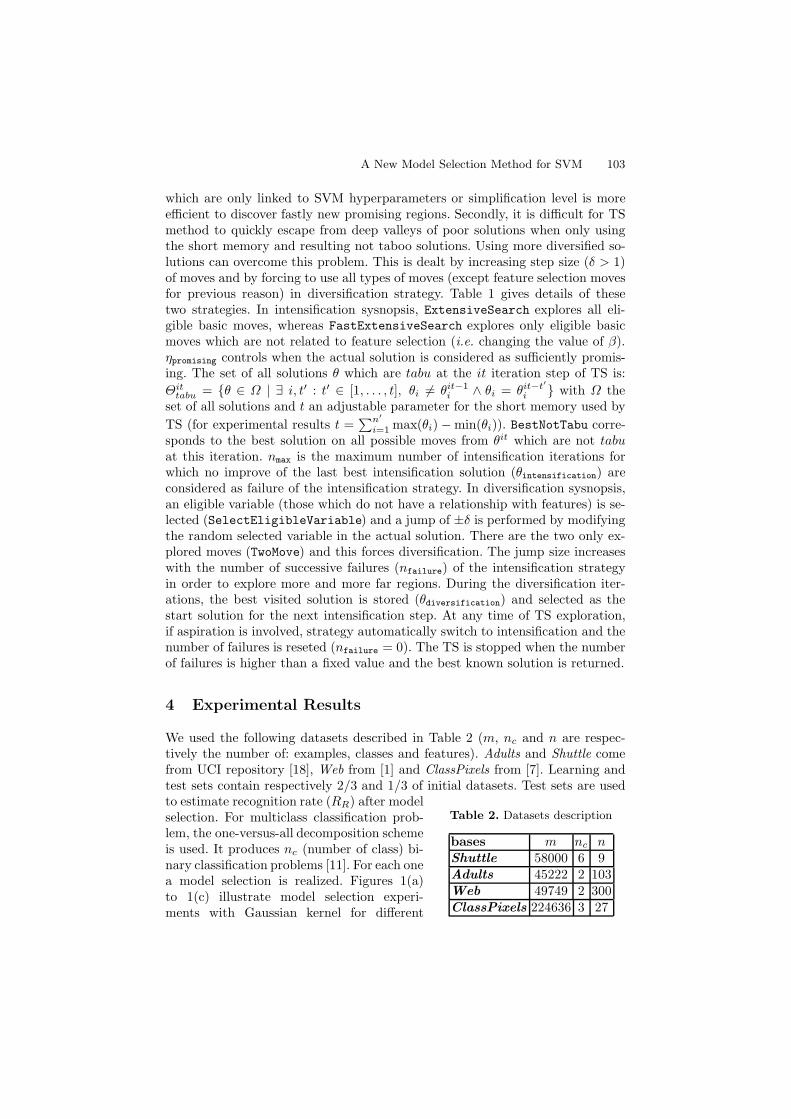
We used the following datasets described in Table 2 (m, nc and n are respec-tively the number of: examples, classes and features). Adults and Shuttle comefrom UCI repository [18], Web from [1] and ClassPixels from [7]. Learning andtest sets contain respectively 2/3 and 1/3 of initial datasets. Test sets are used

Table 2. Datasets description

bases m nc nShuttle 58000 6 9Adults 45222 2 103Web 49749 2 300ClassPixels 224636 3 27

to estimate recognition rate (RR) after modelselection. For multiclass classification prob-lem, the one-versus-all decomposition schemeis used. It produces nc (number of class) bi-nary classification problems [11]. For each onea model selection is realized. Figures 1(a)to 1(c) illustrate model selection experi-ments with Gaussian kernel for different

104 G. Lebrun et al.

0.76

0.78

0.8

0.82

0.84

0.86

0.88

0.9

0.92

0 2 4 6 8 10 12 14

AdultsWeb

(a)

1

10

100

1000

10000

100000

0 2 4 6 8 10 12 14

AdultsWeb

(b)

10

100

1000

10000

100000

1e+006

0 2 4 6 8 10 12 14

AdultsWeb

(c)

Fig. 1. Best recognition rate (a) and number of SVs (b) of BDF for a given simplifi-cation level k. Grid search method are used to select best model (C,σ). (c) gives totaltraining time in seconds for grid search at each simplification level k.

simplification levels. Figure 1(a) shows that the level for which increasing train-ing set size does not significantly improves recognition rate depends on dataset(i.e. importance of redundancy in dataset). Figure 1(c) shows that direct trainingwith the whole dataset is time expensive for model selection. Moreover, complex-ity of decision function (fig. 1(b)) is directly linked to training set size of thisone.

The objective of our learning method is to automatically select different pa-rameters for producing SVM BDF which optimize the DFQ. However new pa-rameters have been introduced and this can be problematic. Next experimentsshow how to deal with them. Our learning method is applied3 on Adults datasetand table 3 (top) shows that an increase of ηpromising reduces the learning timewithout reducing quality of solution. Experiments with other datasets gave thesame results and ηpromising can be fixed at 99%. Similar experiments have shownthat a good compromise between learning time and quality of produced solutionis nmax = 5 and maximum of accepted failure nmax

failure = 5.Tables 3 (middle and bottom) illustrates the complexity evolution obtained

with our learning method by using different penalties (cp1 and cp2). Resultsshow that higher penalties significantly reduce the number of SVs, the numberof selected features and learning time while the recognition rate decrease is lowif penalty is not too high. Of course good compromise depends on the consideredapplication. Another interesting observation for a multiclass SVM scheme is thatselected simplification levels could be different for each binary SVMs (Shuttleset in tab. 3). If training time are compared to the classical grid search methodswithout simplification of training set (fig. 1(c)), training time is greatly reduced(except for very low penality and feature selection) whereas our method preformsin addition feature and simplification level selection. Let nk be the number ofsolutions θ examined by TS for which simplification level is equal to k. GlobalSVM training time of our method is O(

∑nk(2k)γ) with γ ≈ 2. The examination

of our method shows that nk decreases while k increases. This effect increaseswhen cp values increases and explains the efficient training time of our method. In

3 Starting solution is: k = �log2(m/nc)/3�, C′ = 0, σ′ = 0 and nfeature = n.

A New Model Selection Method for SVM 105

Table 3. Top: Influence of ηpromising for model selection (Adults dataset, cp1 = cp2 =10−3). Middle: Trade off between recognition rate and complexity (Adult(A) or Web(W)dataset, ηpromising = 99%). Bottom: Models selection for one-versus-all scheme (Shuttledataset, ηpromising = 99%). For all tables Tlearning is the learning time for model selec-tion in seconds, nfeature is the number of selected features, DFQ is computed on thevalidation dataset (value of RR in DFQ criterion) and selected model RR is evaluatedon a test dataset.

ηpromising Tlearning k log√2(C) log√

2(σ) nVS nfeature RR DFQ99.5 % 6654 6 0 0 50 9 79.3% 0.78999.0 % 9508 1 -3 6 4 22 81.7% 0.80398.0 % 160179 4 0 8 18 20 81.1% 0.80495.0 % 195043 0 10 5 2 41 81.9% 0.8030.0 % 310047 12 1 5 3286 44 81.8% 0.805

with feature selection withoutS cp1 = cp2 Tlearning k nVS nfeature RR DFQ Tlearning k nVS RR DFQA 0.0100 5634 0 2 44 81.5% 0.762 1400 0 2 79.4% 0.789A 0.0020 16095 4 12 44 81.9% 0.793 2685 3 6 79.9% 0.800A 0.0001 127096 10 764 55 81.8% 0.817 7079 13 5274 81.7% 0.811W 0.1000 4762 1 3 44 82.2% 0.598 1736 1 3 84.1% 0.695W 0.0100 25693 2 5 149 87.3% 0.846 4378 5 39 87.5% 0.835W 0.0010 197229 9 506 227 89.7% 0.881 18127 11 730 90.4% 0.898

cp1=cp2= 0.01 cp1=cp2= 0BDF Tlearning k nVS nfeature RR Tlearning k nVS nfeature RR

1-vs-all 207 4 7 2 99.85% 38106 15 127 3 99.83%2-vs-all 67 0 2 1 99.93% 14062 10 20 3 99.95%3-vs-all 45 0 2 1 99.94% 7948 11 38 3 99.95%4-vs-all 152 5 9 2 99.91% 31027 14 63 4 99.94%5-vs-all 44 3 2 1 99.98% 36637 7 13 2 99.96%6-vs-all 113 2 5 1 99.97% 394 6 24 6 99.97%

(a) Microscopic image. (b) Expert segmentation. (c) Pixel classification.

Fig. 2. Pixel classification (RR = 90.1%) using feature extraction cost

our last experiments, pixel classification is performed for microscopical images.On such masses of data, the processing time is critical and we can assign a weightto each color feature of pixel: let κi = n · Ti/T be the weight with Ti the time

106 G. Lebrun et al.

to extract the ith color feature (T =∑

i∈[1,...,n] Ti). With our model selectionmethod, pixel classification (fig. 2) can be performed with only 7 SVs and 4 colorfeatures (see [7] for further details).

5 Conclusions and Discussions

A new learning method is proposed to perform efficient model selection for SVMs.This learning method produces BDFs whose advantages are threefold: high gen-eralization abilities, low complexities and selection of efficient features subsets.Moreover, feature selection can take into account feature extraction cost andmany kinds of kernel functions with less or more hyperparameters can easilybe used. Future works will deal with the influence of other simplification meth-ods [2,6,5]. In particular, because QV methods can be time expensive with hugedatasets.

References

1. Platt, J.: Fast training of SVMs using sequential minimal optimization, advancesin kernel methods-support vector learning. MIT Press (1999) 185–208

2. Yu, H., Yang, J., Han, J.: Classifying large data sets using SVM with hierarchicalclusters. In: SIGKDD. (2003) 306–315

3. Lebrun, G., Charrier, C., Cardot, H.: SVM training time reduction using vectorquantization. In: ICPR. Volume 1. (2004) 160–163

4. Chang, C.C., Lin, C.J.: Libsvm: a library for support vector machines. SofwareAvailable at http://www.csie.ntu.edu.tw/˜cjlin/libsvm (2001)

5. Ou, Y.Y., Chen, C.Y., Hwang, S.C., Oyang, Y.J.: Expediting model selection forSVMs based on data reduction. In: IEEE Proc. SMC. (2003) 786–791

6. Tsang, I.W., Kwok, J.T., Cheung, P.M.: Core vector machines: Fast SVM trainingon very large data sets. JMLR 6 (2005) 363–392

7. Lebrun, G., Charrier, C., Lezoray, O., Meurie, C., Cardot, H.: Fast pixel classifi-cation by SVM using vector quantization, tabu search and hybrid color space. In:CAIP. (2005) 685–692

8. Chapelle, O., Vapnik, V., Bousquet, O., Mukherjee, S.: Choosing multiple para-meters for support vector machines. Machine Learning 46 (2002) 131–159

9. Chapelle, O., Vapnik, V.: Model selection for support vector machines. In: Ad-vances in Neural Information Processing Systems. Volume 12. (1999) 230–236

10. Frohlich, H., Chapelle, O., Scholkopf, B.: Feature selection for support vectormachines using genetic algorithms. IJAIT 13 (2004) 791–800

11. Rifkin, R., Klautau, A.: In defense of one-vs-all classification. JMLR 5 (2004)101–141

12. Christianini, N.: Dimension reduction in text classification with support vectormachines. JMLR 6 (2005) 37–53

13. Gersho, A., Gray, R.M.: Vector Quantization and Signal Compression. KluwerAcademic (1991)

14. Staelin, C.: Parameter selection for support vector machines. http://www.hpl.hp.com/techreports/2002/HPL-2002-354R1.html (2002)

15. Glover, F., Laguna, M.: Tabu search. Kluwer Academic Publishers (1997)

A New Model Selection Method for SVM 107

16. Korycinski, D., Crawford, M.M., Barnes, J.W.: Adaptive feature selection forhyperspectral data analysis. SPIE 5238 (2004) 213–225

17. Vapnik, V.N.: Statistical Learning Theory. Wiley edn. New York (1998)18. Blake, C., Merz, C.: Uci repository of machine learning databases. advances in

kernel methods, support vector learning. (1998)