explicit max margin input feature selection for nonlinear svm …tfcolema/articles/fspaper.pdf ·...

EXPLICIT MAX-MARGIN FEATURE SELECTION

Explicit Max Margin Input Feature Selectionfor Nonlinear SVM using Second Order Methods

Aditya Tayal ∗† [email protected] School of Computer ScienceUniversity of WaterlooWaterloo, ON, Canada N2L 3G1

Thomas F. Coleman †‡ [email protected] and OptimizationUniversity of WaterlooWaterloo, ON, Canada N2L 3G1

Yuying Li † [email protected]

Cheriton School of Computer ScienceUniversity of WaterlooWaterloo, ON, Canada N2L 3G1

Editor: TBA

Abstract

Incorporating feature selection in nonlinear SVMs leads to a large and challenging nonconvex mini-mization problem, which can be prone to suboptimal solutions. We use a second order optimizationmethod that utilizes eigenvalue information and is less likely to get stuck at suboptimal solutions.We devise an alternating optimization approach to tackle the problem efficiently, breaking it downinto a convex subproblem, corresponding to SVM optimization, and a nonconvex subproblem forfeature selection. Importantly, we show that a naive approach, which implicitly maximizes the mar-gin, can be susceptible to saddle point solutions. We propose a new explicit margin maximizationmethod, which overcomes the drawbacks of the implicit approach. To avoid being trapped at saddlepoints, we first introduce an auxiliary variable and perform alternating optimization in the extendedspace, and then subsequently, to improve solution quality, we relax the use of geometric marginand maximize the functional margin in the feature selection subproblem. We demonstrate howthis technique can also be applied to 1-norm linear programming SVMs. Experiment results showthe explicit margin approach works effectively in the presence of class noise and many irrelevantfeatures, consistently outperforming leading filter, wrapper, and other embedded nonlinear featureselection methods.

Keywords: nonlinear feature selection, support vector machine, max margin, saddle point, secondorder method

∗. Corresponding author†. All three authors acknowledge funding from the National Sciences and Engineering Research Council of Canada‡. This author acknowledges funding from the Ophelia Lazaridis University Research Chair. The views expressed

herein are solely from the authors.

1

TAYAL, COLEMAN AND LI

1. Introduction

Feature selection has become a significant research focus in statistical machine learning and datamining communities. As increasingly more data is available, problems with hundreds and eventhousands of input feature variables have become common. Some examples include text processingof internet documents, gene micro-array analysis, combinatorial chemistry, economic forecastingand context based collaborative filtering. However, too many irrelevant features reduce the effec-tiveness of data mining and may detract from the quality and accuracy of the resulting model. Thegoal of input feature selection is to identify the most relevant subset of input features for the learningtask, improving generalization error and model interpretability.

In this paper, we focus on feature selection1 for nonlinear Support Vector Machine (SVM)classification. SVM is based on the principle of maximum-margin separation, which achieves thegoal of Structural Risk Minimization by minimizing a generalization bound on model complexity(VC-dimension) and training error concurrently (Cortes and Vapnik, 1995; Vapnik, 1998). Themodel is obtained by solving a convex quadratic programming problem. Linear SVM models canbe extended to nonlinear ones by transforming the input feature space using a set of nonlinear basisfunctions. An important advantage of the SVM is that the transformation can be done implicitlyusing the “kernel trick”, thereby allowing even infinite-dimensional feature expansions (Boser et al.,1992). Empirically, SVMs have performed extremely well in diverse domains (e.g. see Byun andLee, 2002; Scholkopf et al., 2004).

Many feature selection methods have been proposed for linear SVMs based on sparse regular-ization of the primal weight vector. For instance Bradley and Mangasarian (1998); Zhu et al. (2003);Fung and Mangasarian (2004) propose an `1-norm as the regularizer, while Weston et al. (2003);Chan et al. (2007); Tan et al. (2010) directly approximate or convexify the zero norm of the weightvector. However, similar techniques cannot be readily applied to nonlinear SVM classifiers, sincethe weight vector no longer corresponds to input features directly. In this case, sparse regularizationwould lead to a reduction in the dimensionality of the higher dimensional transformed space or inthe number of kernel functions needed to generate the nonlinear surface (Fung and Mangasarian,2004), but does not result in a reduction of input space features.

In the literature there has been comparatively little emphasis on feature selection for nonlin-ear SVMs, despite their efficacy as universal predictors. Furthermore, when covariates are relatednon-linearly, noisy features that contain little or no information can critically impair generalizationperformance. As an illustration, Figure 1c shows test error degradation as number of noise fea-tures are added to a simple linear (Figure 1a) and nonlinear dataset (Figure 1b). The linear datasetis comparatively robust to small number of irrelevant features, while almost all modeling ability isquickly lost in the nonlinear dataset. Consequently, feature selection can be imperative for nonlinearmodels—where it also becomes a significantly more difficult task.

Theoretically, determining the optimal set of features is NP-hard, requiring an exhaustive searchof all possible subsets of features. Practical alternatives can be grouped into filter, wrapper, and em-bedded categories (Guyon and Elisseeff, 2003). Filter methods operate independently of the SVMclassifier to score features according to how useful they are in predicting the output. Relief (Kira

1. Subsequently, the term feature selection refers to the input feature selection, rather than selection of features in thederived feature space using kernel mapping.

2


(a) (b)

0 1 2 5 10 200

10

20

30

40

50

Number of noise features

Te

st

err

or

(%)

Linear

Nonlinear

(c)

Figure 1: Simple two-dimensional separable (a) linear and (b) nonlinear datasets are used to com-pare the effect of noisy features on classification accuracy. (c) Generalization error de-grades more drastically for the nonlinear dataset compared to the linear one as additionalnoise features are added. In both cases an SVM model is learned using the Gaussiankernel, where the kernel width parameter is tuned using cross-validation.

and Rendell, 1992; Sikonja and Kononenko, 2003) is a popular nonlinear filter that has successfullybeen used as a preprocessing step for SVMs (e.g. see Marchiori, 2005). Wrapper methods use theSVM classifier to guide the search in the space of all possible subsets. For instance the most com-mon wrapper, recursive feature elimination, greedily removes the worst (or adds the best) featureaccording to the loss (or gain) of the SVM classifier at each iteration (Guyon et al., 2002). Em-bedded approaches incorporate the feature selection criterion in the SVM objective itself, and canoffer significant advantages compared to filter and wrapper methods, since they are tailored to theSVM classifier and can take into account complex nonlinear dependencies to ensure no informationis lost. Weston et al. (2000) propose an embedded feature selection method that minimizes the ex-pected error bound using gradient descent based on the dual SVM objective. Mangasarian and Kou(2007) use a mixed-integer algorithm to reduce the number of input features in a nonlinear SVMclassifier.

Incorporating feature selection in nonlinear SVMs results in a nonconvex optimization problem.Indeed, nonconvexity is one of the main challenges of nonlinear feature selection, particularly forhighly nonlinear kernels, such as the Gaussian kernel. We illustrate that heuristic methods, such asRelief and Recursive Feature Elimination, and first-order optimization techniques, such as gradi-ent descent, can be prone to suboptimal solutions. Consequently, in order to obtain robust resultsin a variety of circumstances, we use a second order minimization approach which explicitly com-putes eigenvectors associated with the minimum eigenvalues to solve an embedded feature selectionproblem for nonlinear SVMs.

We embed the feature selection process into the primal nonlinear SVM by replacing kernel in-puts with a weighted input vector, while imposing an `1 penalty on the weights to encourage featuresparsity. This results in a large continuous but nonconvex minimization problem in the space ofSVM model parameters and feature weights. We propose an alternating optimization approach to

3


tackle the problem efficiently, breaking it down into a convex subproblem, corresponding to SVMoptimization, and a reduced non-convex subproblem, for feature selection. To solve the featureselection subproblem, we use a trust region algorithm for the bound constrained minimization prob-lem; this trust region method computes eigenvectors of the Hessian corresponding to the most neg-ative curvature in order to avoid being trapped at saddle points of the objective function (Colemanand Li, 1996). We use a smoothed hinge-loss cost function to make the objective function contin-uously differentiable. However, we show that a naive approach, which solves the feature selectionsubproblem by implicitly maximizing the margin, can be ineffective and susceptible to saddle pointsolutions within an alternating optimization setup. One of our key contributions, which overcomesthe drawbacks of the implicit approach, is proposing a new method for feature selection based onexplicit margin maximization. We develop the formulation in two stages: first, we introduce anauxiliary variable using perspective mapping and perform alternating optimization in the extendedspace, and then subsequently, we relax the use of geometric margin and maximize the functionalmargin in the feature selection subproblem. We demonstrate how this technique can also be appliedto 1-norm linear programming SVMs. Finally, we computationally confirm that the explicit max-margin approach is effective for nonlinear kernels in the presence of class noise and many irrelevantfeatures, consistently outperforming leading filter, wrapper, and other embedded feature selectionmethods on simulated and real datasets.

The rest of the paper is organized as follows. Section 2 formulates the embedded feature selec-tion problem. Section 3 describes a second order minimization approach for feature selection. Sec-tion 4 discusses alternating optimization using a smoothed hinge loss function and an implicit mar-gin for feature selection. Section 5 develops the explicit max-margin formulation which remediesthe shortcomings of the implicit approach. Section 6 develops the explicit max-margin approach for1-norm linear programming SVMs. Section 7 compares our methods with other nonlinear featureselection approaches computationally and we conclude with a discussion in Section 8.

2. Max-Margin Feature Selection

We start by formulating an embedded feature selection problem for standard support vector ma-chines. We motivate and explain the formulation with respect to generalization bounds.

Consider a set of n training points, xi ∈ Rd , and corresponding class labels, yi ∈ +1,−1,i = 1, ...,n. Here each component of xi is an input feature. We solve for an optimal classifier withinthe max-margin framework. In the classical SVM, proposed by Cortes and Vapnik (1995), we learna linear classifier (w,b) by maximizing the geometric margin, defined as γ ≡mini yi(wT xi+b)/‖w‖,where ‖ · ‖ denotes 2-norm. Since the decision hyperplane associated with (w,b) does not changeupon rescaling to (λw,λb), for λ ∈ R+, we can fix the function output at the margin (functionalmargin) to 1, so geometric margin is given by γ = 1/‖w‖, and we minimize the norm of the weightvector. Thus in the standard setting, with all features used, SVM results in the following convex

4


quadratic programming problem:

minw,b,ξ

12‖w‖2 +C

n

∑i=1

ξi,

s.t. yi(wT xi +b

)≥ 1−ξi, i = 1, ...,n, (1)

ξi ≥ 0, i = 1, ...,n ,

where ξi’s are slack variables when training instances are not linearly separable and C is a penalty,associated with margin violations, which determines the trade-off between accuracy and modelcomplexity.

To obtain a non-linear decision function we use the kernel trick (Boser et al., 1992) by defininga kernel function, K(x,x′) ≡ φ(x)T

φ(x′), where K : Rd ×Rd → R and φ : Rd → F is a non-linearmap from the input space to a (potentially infinite dimensional) feature space derived from featureinputs. A kernel function, satisfying Mercer’s condition (Mercer, 1909; Courant and Hilbert, 1953),directly computes the inner product of two vectors in the (derived) feature space, without the need toexplicitly determine the feature mapping. Conventionally, the kernel is used in the dual of problem(1), where all occurrences of data appear inside an inner product. However, we can also formu-late the primal problem in feature space by expressing the weight vector as a linear combination ofmapped data points, w = ∑

ni=1 yiuiφ(xi), due to Representer theorem (Scholkopf and Smola, 2002).

Here we denote the coefficients as ui, not αi used in the standard SVM literature, in order to distin-guish them from the typical Lagrange multiplier interpretation. Substituting this form in (1) leadsto the following non-linear SVM problem,

minu,b,ξ

12

n

∑i, j=1

yiy juiu jK(xi,x j)+Cn

∑i=1

ξi,

s.t. yi

(n

∑j=1

y ju jK(xi,x j)+b

)≥ 1−ξi, i = 1, ...,n, (2)

ξi ≥ 0, i = 1, ...,n ,

with a geometric margin in feature space given by

γ =1√

∑ni, j=1 yiy juiu jK(xi,x j)

.

The dual of problem (2) reveals that the primal variable ui is equivalent to the standard SVM dualLagrange multiplier αi, i.e. ui = αi, when the kernel matrix is non-singular. If the kernel matrix issingular, then the coefficient expansion ui is not unique (even though the decision function is) andsolving (2) will produce one of the possible expansions, of which αi is also a minimizer.

The maximum margin classifier is motivated by theoretical bounds on the generalization error.Specifically, Vapnik (1998) shows that generalization error for n points is bounded by,

err ≤ cn

[(R2

γ2 +‖ξ‖2)

log2 n+ log1δ

], (3)

5


for some constant c with probability 1− δ , where γ is the geometric margin of the classifier. Thekey expression, on which generalization depends, is R2/γ2 + ‖ξ‖2, where ξ is the margin slackvector (normalized by γ), and R is the radius of the ball that encloses the set of points in the derivedfeature space, φ(xi)n

i=1. For a fixed dataset and kernel choice, R is constant, and thus maximizingthe margin while reducing margin violations minimizes the upper bound in (3). Although the gener-alization bound suggests using a 2-norm penalty on margin violations, a 1-norm penalty is preferredfor classification tasks, since it is a better approximation to a step penalty. Thus the parameter C in(2) controls the tradeoff between margin maximization versus margin violations; this parameter isgenerally determined by cross-validation.

Consider learning such a classifier where input features are weighted according to their rele-vance. We introduce a feature weight vector, z ∈ Rd , where zl ≥ 0 is a weight applied to inputfeature l. For convenience we define a diagonal matrix, Z ∈ Rd×d with Zll = zl . Hence, weightedpoints are mapped to φ(Zx) and we can replace K(x,x′) by K(Zx,Zx′) in problem (2) to obtainan embedded feature selection problem, in which we simultaneously search for optimal featureweights, z, while solving for model parameters, (u,b):

minu,b,ξ ,z

12

n

∑i, j=1

yiy juiu jK(Zxi,Zx j)+Cn

∑i=1

ξi +µ‖z‖1,

s.t. yi

(n

∑j=1

y ju jK(Zxi,Zx j)+b

)≥ 1−ξi, i = 1, ...,n, (4)

ξi ≥ 0, i = 1, ...,n,

zl ≥ 0, l = 1, ...,d .

Here, we have also included a 1-norm feature regularization term in the objective with a penaltyparameter µ > 0. This serves two purposes. Firstly, the 1-norm regularizer has the beneficial effectof suppressing features to produce a sparse set of non-zero feature weights (Tibshirani, 1996). Thisproperty is desirable for feature selection where we are interested in identifying the most usefulsubset of input features. Secondly, it acts to minimize the radius of the enclosing ball, R, for thegeneralization bound in (3). Given two feature weight vectors, z and z′, if z′l ≤ zl , for l = 1, ...,d, then∑l z′2l (xil−x jl)

2≤∑l z2l (xik−x jl)

2, implying ‖Z′xi−Z′x j‖≤ ‖Zxi−Zx j‖. Thus suppressing featureweights tend to reduce distances between points in input space, which in turn results in a smallerenclosing ball in feature space. Consequently, once we allow feature weights to vary, R is no longerconstant. Figure 2 illustrates this effect using the Gaussian kernel for a randomly generated two-dimensional dataset. The inscribing ball radius R is computed as described in Weston et al. (2000).From subplot (b) we observe that a smaller ‖z‖1 is associated with a smaller R. To minimize thegeneralization bound, we can solve (4) and calibrate margin, errors, and radius using parameters Cand µ , which can be determined by cross-validation.

3. Second-order Nonconvex Minimization for Feature Selection

In the feature selection problem (4), the objective function and constraints are convex with respectto u,b,ξ , for fixed feature z, but non-convex with respect to feature weight z for a nonlinear SVM.Consider a Gaussian kernel for a single feature, for example, the classifier involves a function of the

6


−2 −1 0 1 2−3

−2

−1

0

1

2

x1

x2

(a) (b)

Figure 2: (a) Random sample points generated using a mixture of normals on a two-dimensionalplane. (b) The minimum enclosing radius, R, of the points in feature space, using a Gaus-sian kernel, as a function of feature weights, z1 and z2 (blue surface). Suppressing featureweights using ||z||1 (gray transparent surface) has the effect of minimizing R2 in featurespace.

form −e−ρz2with ρ > 0, which is nonconvex in z. A first order optimization method, or a second

order method which does not utilize the minimum eigenvalue and eigenvector, can terminate at asaddle point of the objective function. Indeed, to effectively obtain optimal features, we believethat using a second order minimization method, which incorporates information on the minimumeigenvalue of the Hessian, is crucial for robust feature selection.

A trust region minimization method for unconstrained minimization solves a subproblem belowat each iteration (indexed by k):

mins∈Rm

sT gk +12

sT Hks (5)

s.t. ‖s‖2 ≤ ∆k

where gk and Hk are gradient and Hessian of the objective function with m variables. For a noncon-vex minimization problem, the Hessian Hk can be indefinite and the trust region subproblem (5) is anonconvex quadratic minimization problem with a ball constraint. However, a global minimizer ofthis subproblem can be computed since there is no duality gap for a trust region subproblem, evenwhen it is nonconvex. For example, assuming ∆k = 1 for simplicity, the dual of the trust regionsubproblem (5) can be solved by first computing a solution to

maxυ∈R

−d

∑i=1

(qTi gk)2

υi +υ−υ (6)

s.t. υ ≥−υmin(Hk)

7


where υi and qi are the eigenvalues and corresponding orthonormal eigenvectors of Hk respectively,and υ(Hk) denotes the minimum eigenvalue of Hk (Boyd and Vandenberghe, 2004).

Although solving a trust region subproblem is computationally expensive, the optimization it-erates are guaranteed to converge to a solution ensuring the Hessian becomes positive semidefinite.Trust region methods have strong convergence properties and are robust, even when problems areill-conditioned (Yuan, 2000). In addition, by incorporating directions associated with minimumeigenvalues, the iterates have better chance of reaching a global minimum for a nonconvex mini-mization problem.

We believe that it is important to use a second order method which exploits the curvature in-formation of the objective function Hessian for robust feature selection. For our subsequent com-putational results, we solve the feature selection problem using the trust-region method for boundconstraints proposed in Coleman and Li (1996).

Computational results in this paper are obtained using an implementation which solves a trustsubproblem using an eigen-decomposition of the Hessian matrix, effectively costing O(m3) opera-tions for a specified accuracy tolerance. The trust region subproblem can also be computed usingCholesky factorizations of the Hessian, costing O(m3) operations for each factorization. Thus theapproach is more suitable for small to medium number of features. For larger problems, an approxi-mate subspace trust-region approach can be used (Branch et al., 1999). In this case, the trust-regionsubproblem is restricted to a two-dimensional subspace, consisting of the gradient and either anapproximate Newton direction or a direction of negative curvature obtained by a conjugate gradientprocess. Alternatively the trust region subproblem can also be computed by reformulating it as aparameterized eigenvalue problem, which can be solved using a matrix-free method with matrix-vector product computations (Rojas et al., 2008).

4. Alternating Optimization Approach

For a data set with a large number of the data points, n, it is computationally challenging to solvethe feature selection problem (4) with O(n+d) number of variables, even when the number of theinput features d is relatively small. For computational efficiency, we first exploit the structure ofthe feature selection problem (4) by developing an alternating optimization method using a naiveimplicit max-margin approach. We then discuss its limitations and improve the approach further bydeveloping an explicit max-margin formulation in Section 5.

We would like to take advantage of the fact that for fixed feature weights, problem (4) reducesto a convex problem that corresponds to regular SVM optimization, which can be solved very effi-ciently (e.g. see Platt, 1999; Fan et al., 2005). Thus we propose a two-block alternating optimiza-tion (AO) approach (also known as nonlinear block coordinate descent or Gauss-Seidel method), inwhich we iterate between (a) fixing feature weights and solving an SVM problem for model param-eters (u,b), and (b) fixing model parameters and solving a smaller non-convex problem for featureweights, z. Formally, we write problem (4) as

minu,b,z

Ψ(u,b,z),12

n

∑i, j=1


∑i=1

Vi(u,b,z)+µ‖z‖1, (7)

s.t. zl ≥ 0, l = 1, ...,d .

8


where V is the hinge loss function,

Vi(u,b,z) = max

(0,1− yi

(n

∑j=1

y ju jK(Zxi,Zx j)+b

)), (8)

Then AO entails solving the following two subproblems iteratively as follows: starting from aninitial feature vector, z0 ≥ 0, we solve

(a) SVM subproblem: (uk,bk) = argminu,b

Ψ(u,b,zk) (9)

(b) Feature selection subproblem: zk+1 = argminz≥0

Ψ(uk,bk,z) , (10)

This generates a sequence (uk,bk,zk)∞k=1 yielding a sequence of objective values Ψ(uk,bk,zk)∞

k=1,which converges following from the fact that the sequence is nonincreasing and bounded below byzero. Moreover, every limit point of (uk,bk,zk) is a critical point of problem (7), since for atwo-block decomposition it can be shown that limit points of the partial updates generated by AOare critical points with respect to both sets of variables. The proof is based on the fact that theminimum value in a component subspace is lower than the function value obtainable through a con-vergent Armijo-type line search (Grippo and Sciandrone, 2000).2 Computationally, the algorithmcan be terminated when successive changes in the variables are less than a prespecified tolerance:‖(∆uk+1,∆bk+1,∆zk+1)‖∞ < tol, where (∆uk+1,∆bk+1,∆zk+1) = (uk+1−uk,bk+1−bk,zk+1− zk).

The AO approach decomposes problem (7) into two subproblems (9) and (10), which can besolved more efficiently. Problem (9) is a standard SVM problem and can be solved by convexquadratic optimization techniques. Problem (10) optimizes features for fixed model parameters,by implicitly maximizing the margin, via minimizing ∑

ni, j=1 yiy juiu jK(Zxi,Zx j), while penalizing

for error and radius. We refer to solving (9) and (10) iteratively as the implicit max-margin AOapproach since the geometric margin is implicit in subproblems.

4.1 Smoothed hinge loss

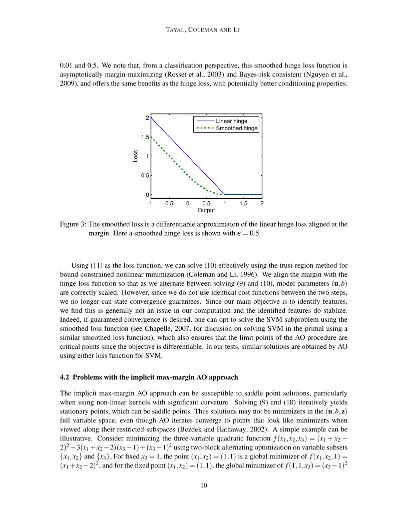
The linear hinge loss function max(0,1− r) for an output r, used in (8), is not differentiable. Alter-native differentiable loss functions can be used instead. In this paper we consider a smoothed hingeloss function ρε(1− r) so that problem (10) becomes a smooth minimization problem with simplebound constraints. The continuous differentiable smoothed hinge loss function is (see Figure 3):

ρε(t)≡

t− ε if t > 2ε

14ε

t2 if 0 < t ≤ 2ε

0 otherwise .

(11)

The function transitions from a linear cost to zero cost using a quadratic segment and bears similarityto the Huber loss. Here, ε controls the amount of smoothing and is generally chosen to be between

2. Strictly speaking, to apply this result we require Ψ(·) to be differentiable. We address this in the Section 4.1, wherewe propose a smooth differentiable hinge loss approximation.

9


0.01 and 0.5. We note that, from a classification perspective, this smoothed hinge loss function isasymptotically margin-maximizing (Rosset et al., 2003) and Bayes-risk consistent (Nguyen et al.,2009), and offers the same benefits as the hinge loss, with potentially better conditioning properties.

−1 −0.5 0 0.5 1 1.5 2

0

0.5

1

1.5

2

Output

Loss

Linear hinge

Smoothed hinge

Figure 3: The smoothed loss is a differentiable approximation of the linear hinge loss aligned at themargin. Here a smoothed hinge loss is shown with ε = 0.5.

Using (11) as the loss function, we can solve (10) effectively using the trust-region method forbound-constrained nonlinear minimization (Coleman and Li, 1996). We align the margin with thehinge loss function so that as we alternate between solving (9) and (10), model parameters (u,b)are correctly scaled. However, since we do not use identical cost functions between the two steps,we no longer can state convergence guarantees. Since our main objective is to identify features,we find this is generally not an issue in our computation and the identified features do stablize.Indeed, if guaranteed convergence is desired, one can opt to solve the SVM subproblem using thesmoothed loss function (see Chapelle, 2007, for discusion on solving SVM in the primal using asimilar smoothed loss function), which also ensures that the limit points of the AO procedure arecritical points since the objective is differentiable. In our tests, similar solutions are obtained by AOusing either loss function for SVM.

4.2 Problems with the implicit max-margin AO approach

The implicit max-margin AO approach can be susceptible to saddle point solutions, particularlywhen using non-linear kernels with significant curvature. Solving (9) and (10) iteratively yieldsstationary points, which can be saddle points. Thus solutions may not be minimizers in the (u,b,z)full variable space, even though AO iterates converge to points that look like minimizers whenviewed along their restricted subspaces (Bezdek and Hathaway, 2002). A simple example can beillustrative. Consider minimizing the three-variable quadratic function f (x1,x2,x3) = (x1 + x2−2)2−3(x1+x2−2)(x3−1)+(x3−1)2 using two-block alternating optimization on variable subsetsx1,x2 and x3, For fixed x3 = 1, the point (x1,x2) = (1,1) is a global minimizer of f (x1,x2,1) =(x1+x2−2)2, and for the fixed point (x1,x2) = (1,1), the global minimizer of f (1,1,x3) = (x3−1)2

10


is x3 = 1. Consequently, alternating optimization between the two variable subsets can converge tothe point (x1,x2,x3) = (1,1,1), which is a saddle point of the full-variable space.3

We experimentally illustrate that saddle point convergence in the implicit max-margin methodcan be problematic. Table 1 shows the test error obtained on the NDCC (Normally DistributedClusters on Cubes) dataset as the number of irrelevant features (probes) are increased. NDCC is achallenging highly non-linear dataset consisting of 20 true features. Parameters C and µ are tunedusing a validation set. Models are learned using a Gaussian kernel with σ = 1. The AO processterminates when ‖∆zk+1‖∞ < 5×10−3. Section 7 describes the data and experiment setup in furtherdetails. We see the implicit approach is unable to identify the correct set of features: generaliza-tion error deteriorates quickly as the number of probes increases. In addition, adjacent to each testscore we indicate whether the projected Hessian at termination is positive definite (i.e. υmin > 0),indicated by (M), or indefinite (υmin <−0.1 for this experiment), indicated by (S). We find that theprojected Hessian is indefinite at most computed solutions, suggesting the saddle point possibility.

No. of Probes 0 2 5 10 20 50 100

Test Error 8.3 (M) 8.9 (S) 19.1 (S) 44.9 (S) 52.0 (S) 50.0 (S) 47.5 (S)

Table 1: Test error in percent using the implicit max-margin approach as additional probe featuresare included in the 20-dimension NDCC dataset. Label (M) indicates that, at termination,the projected Hessian is positive semi-definite while label (S) indicates that the projectedHessian is indefinite. Bolded values indicate the correct set of features are identified by themethod.

5. Explicit Max-Margin

In this section we develop an explicit max-margin feature selection method in order to further im-prove the naive implicit max-margin approach and increase the possibility of convergence to a globalminimum. We develop the formulation in two stages. First, in Section 5.1, we extend the featureselection subproblem with an explicit margin variable and then in Section 5.2 we relax the marginterm so it is not tied to the geometric margin.

5.1 Extended subspace

We return to the simple 3-variable example in Section 4.2. We introduce a perspective transforma-tion x1 = x1/y and x2 = x2/y and define f (x1, x2,x3,y) = (yx1 + yx2− 2)2− 3(yx1 + yx2− 2)(x3−1) + (x3 − 1)2. Clearly f (x1, x2,x3,1) = f (x1,x2,x3), i.e., f (x1,x2,x3) is the result of applyinga perspective mapping to normalize the y-component. We now apply AO process to minimizef (x1, x2,x3,y) but with the y variable shared between alternating optimization as follows. We mini-mize f (x1, x2,x3,y) using AO over the variable subsets x1, x2,y and x3,y. For fixed x3 = 1, we

3. The Hessian at (x1,x2,x3) = (1,1,1) contains both positive and negative eigenvalues. Also, see Section 5.1 whichexpands on this example.

11


set y = 1 (since y can be arbitrarily scaled) and minimize f (x1, x2,1,1) = (x1 + x2−2)2 , to obtainthe global minimizer (x1, x2) = (1,1) as before. However, for fixed (x1, x2) = (1,1), we now mini-mize f (1,1,x3,y) = 4(y−2)2−6(y−2)(x3−1)+(x3−1)2 to find that the Hessian of the quadraticfunction with respect to (x3,y) is indefinite. Thus, by extending the subspace with an auxiliaryvariable in this fashion and sharing the variable between AO iterates, a minimization method whichutilizes negative curvature information will lead iterates away from the saddle point.

Motivated by this idea, we introduce an explicit margin variable, λ ≥ 0, in the embedded featureselection problem. We substitute u = u/λ and b = b/λ in problem (4) to obtain,

minu,b,ξ ,λ ,z

12λ 2

n

∑i, j=1


∑i=1

ξi +µ‖z‖1,

s.t. yi

(n

∑j=1

y ju jK(Zxi,Zx j)+ b

)≥ λ −λξi, i = 1, ...,n, (12)

ξi ≥ 0, i = 1, ...,n,

zl ≥ 0, l = 1, ...,d,

λ ≥ 0 .

and optimize over u and λ instead of u. Note, λ represents the functional margin, while ξi’s are theproportional violations from the margin boundary. The geometric margin is scaled by the functionalmargin, γ = λ/

√∑

ni, j=1 yiy juiu jK(xi,x j), and is maximized in the first term of the objective. For the

feature selection subproblem, when model parameters (u, b) are fixed, λ provides an additional viewof the margin component. This allows a larger subspace search to maximize margin and reduces thepossibility of being trapped at a saddle point.

Expressing (12) in the exact-penalty form we obtain

minu,b,λ ,z

Φ(u, b,λ ,z),1

2λ 2

n

∑i, j=1


∑i=1

Vi

(uλ,

bλ,z)+µ‖z‖1, (13)

s.t. zl ≥ 0, l = 1, ...,d,

λ ≥ 0 .

where V is the hinge loss given by (8). In this case, when using AO we share the λ margin variable,solving the following two subproblems iteratively,

(a) Extended SVM subproblem: (uk, bk, λ ) = argminu,b

Φ(u, b,λ ,zk) (14)

(b) Extended FS subproblem: (λ k+1,zk+1) = argminλ ,z≥0

Φ(uk, bk,λ ,z) starting from λ . (15)

We refer to this as the extended subspace feature selection approach. To solve (15), we replacethe hinge loss with the the smoothed cost function given by (11), and use the trust-region interiorreflective algorithm for bound constraints. The AO process has similar convergence properties asthe implicit max-margin approach discussed in Section 4, when a smoothed loss function is usedfor both the SVM and extended feature selection subproblems.

12


For fixed z, problem (14) reduces to solving a regular SVM optimization. By substituting backu = uλ and b = bλ we obtain the standard SVM formulation, which we solve to obtain (u,b). Sinceλ can be arbitrarily scaled by a positive value without changing the subproblem, we set λ = 1 andobtain a unique solution (u, b) = (u,b).

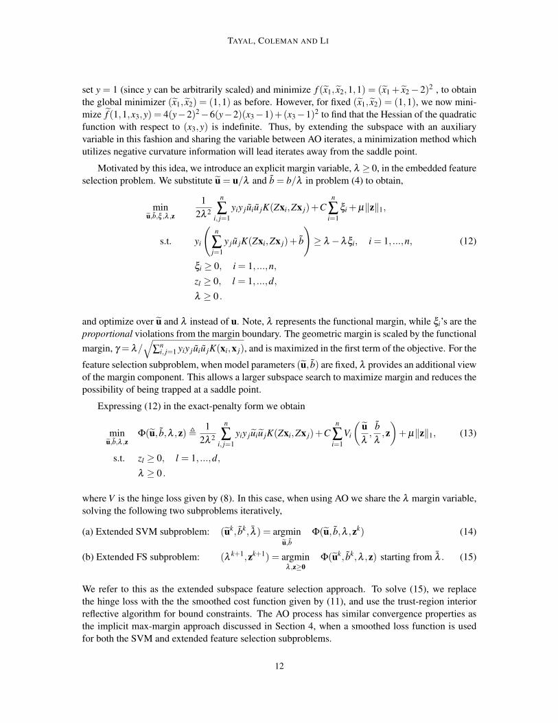
Experiment results confirm that the extended subspace method is indeed able to circumventsaddle point solutions and obtain better generalization error than the implicit max-margin approach.Table 2 shows test error for the NDCC datasets, where (M) or (S) are used to indicate whether theprojected Hessian is positive definite or indefinite. The same AO termination criterion used in Table1 is used for Table 2.

No. of Probes 0 2 5 10 20 50 100

Test Error 9.4 (M) 10.7 (M) 17.5 (M) 11.2 (M) 10.4 (M) 48.0 (M) 45.9 (M)

Table 2: Test error in percent using the extended max-margin approach as additional probe featuresare included in the 20-dimension NDCC dataset. Label (M) indicates that, at termina-tion, the projected Hessian is positive definite while label (S) indicates that it is indefinite.Bolded values indicate the correct set of features are identified by the model.

There are two main observations that we can draw from the results. Firstly, the computedsolutions are no longer at saddle points. We see this improves the ability to identify the correctsubset of features and recover generalization error to some extent. Secondly, despite nonnegativeminimum eigenvalues for the Hessian at termination, the method becomes ineffective when thereare a large number of probes, as indicated by test error and the inability to identify the correctfeatures when there are 50 or 100 probes. In the next section we discuss a further improvement tothe method.

5.2 Function margin maximization in the feature selection subproblem

The feature selection subproblem (15) determines (λ k+1,zk+1) by solving

minλ∈R+,z

12λ 2

n

∑i, j=1

yiy juki uk

jK(Zxi,Zx j)+Cn

∑i=1

V(

uk

λ,bk

λ,z)+µ‖z‖1, (16)

s.t. zl ≥ 0, l = 1, ...,d,

The first term in the objective function equals 12γ2 where γ is the geometric margin; specifically,

1γ2 =

1λ 2

n

∑i, j=1

yiy juki uk

jK(Zxi,Zx j) or equivalently γ = λ/

√n

∑i, j=1

yiy juki uk

jK(xi,x j).

The reason that geometric margin, rather than functional margin, is minimized in the standard SVMis due to the fact that support vector weights are not unique but the decision surface does not changeupon scaling. A 2-norm normalization leads to geometric margin maximization. This normalization

13


yields an alternative formulation for the feature selection subproblem below:

minλ∈R+,z

12λ 2 +C

n

∑i=1

V(

uk

λ,bk

λ,z)+µ‖z‖1, (17)

s.t. zl ≥ 0, l = 1, ...,d,n

∑i, j=1

yiy juki uk

jK(Zxi,Zx j) = 1

where the equality constraint enforces γ = λ .

In the feature selection subproblem, the SVM weights are fixed and the equality constraint isnot necessary, since we do not need to fix the scale of support vectors to maximize margin. Indeed,fixing uk in the feature selection subproblem assumes implicitly that features are selected withidentified support vectors fixed. Thus, geometric margin continues to be measured with respect tothe set of support vectors identified in the prior SVM subproblem. This unnecessary restriction inthe feature selection subproblem can make it difficult to reduce or eliminate unwanted features.

Consequently, we relax feature selection problem (17) by removing the normalization equalityconstraint and obtain the following explicit max-margin feature selection subproblem,

minλ ,z

12λ 2 +C

n

∑i=1

V(

uλ,

bλ,z)+µ‖z‖1, (18)

s.t. zl ≥ 0, l = 1, ...,d,

λ ≥ 0 ,

Thus, problem (18) maximizes the functional margin, λ , instead of geometric margin while modelparameters u are fixed. Since we no longer use the norm to maximize margin, support vectorsthat fall on the margin are free to move outside (or inside) the geometric margin as feature weightschange. Maximizing the functional margin explicitly permits greater flexibility in the feature weightsubproblem, and as a result, we can make better improvement in reducing margin error in the featureweight space and avoid being trapped at suboptimal local minima.

We alternate between solving the SVM subproblem (14) and the explicit margin feature selec-tion subproblem (18). As before, to solve (18) we replace the hinge loss V with the smoothed lossfunction given by (11) and use the trust-region interior reflective algorithm for bound constraints.Since the AO iterates no longer share a common objective, we cannot state any convergence guar-antees, even when the SVM subproblem uses a smoothed loss function. Therefore, we use a weakerstopping criterion for AO iterates that works in practice: ‖∆zk+1)‖0 = 0, where ∆zk+1 = zk+1− zk

and a component is zero if its absolute value is less than 10−2. This criterion is also reasonable sincewe are mainly interested in feature selection in this paper. Usually, only a few (4 ∼ 5) AO iteratesare required, making the approach efficient for large n when training SVMs can be expensive.

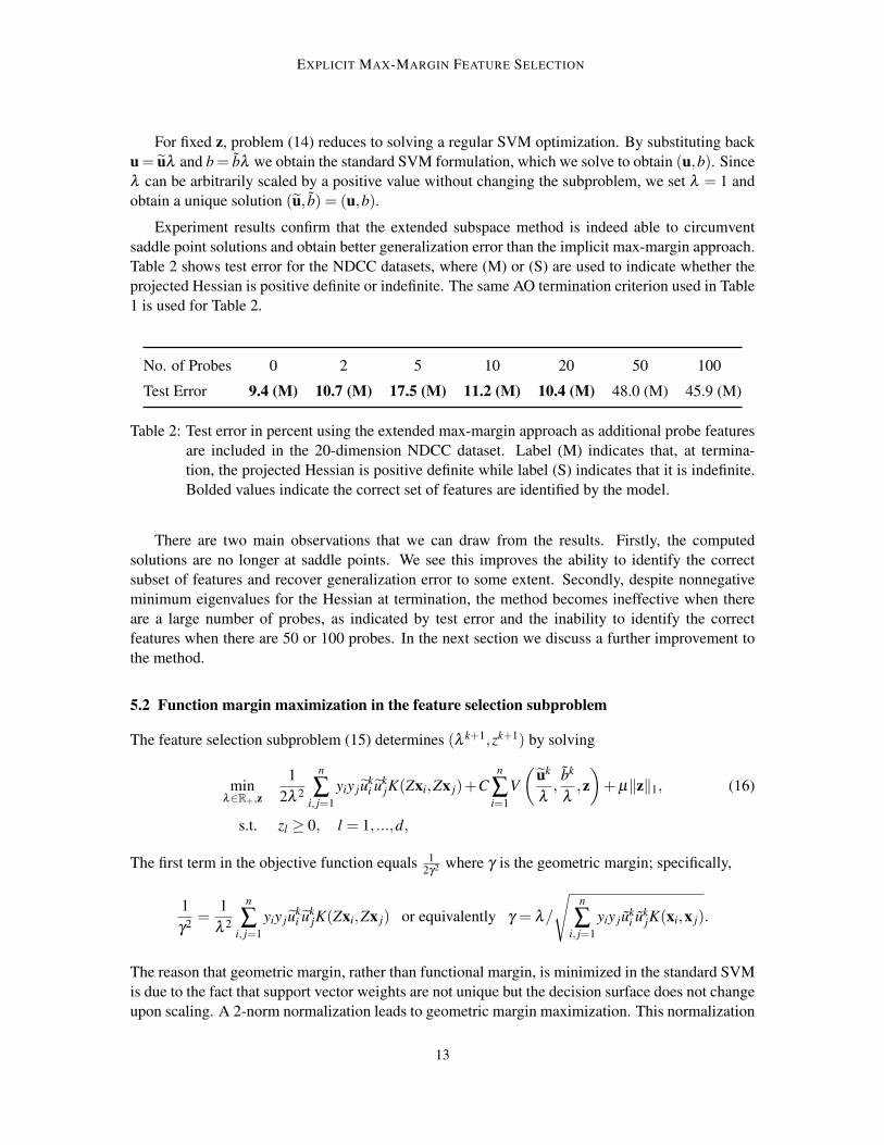
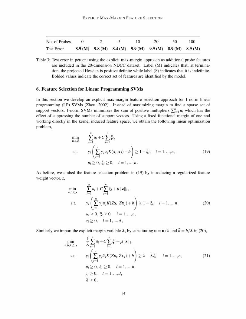
Table 3 shows test error for the NDCC datasets using the explicit margin approach. The methodcontinues to avoid saddle points. In addition, compared to the extended approach (Table 2), themethod can effectively identify the correct set of features and recover a competitive generalizationerror even as the number of probe features become substantial.

14


No. of Probes 0 2 5 10 20 50 100

Test Error 8.9 (M) 9.8 (M) 8.4 (M) 9.9 (M) 9.9 (M) 8.9 (M) 8.9 (M)

Table 3: Test error in percent using the explicit max-margin approach as additional probe featuresare included in the 20-dimension NDCC dataset. Label (M) indicates that, at termina-tion, the projected Hessian is positive definite while label (S) indicates that it is indefinite.Bolded values indicate the correct set of features are identified by the model.

6. Feature Selection for Linear Programming SVMs

In this section we develop an explicit max-margin feature selection approach for 1-norm linearprogramming (LP) SVMs (Zhou, 2002). Instead of maximizing margin to find a sparse set ofsupport vectors, 1-norm SVMs minimizes the sum of positive multipliers ∑

ni=1 ui which has the

effect of suppressing the number of support vectors. Using a fixed functional margin of one andworking directly in the kernel induced feature space, we obtain the following linear optimizationproblem,

minu,b,ξ

n

∑i=1

ui +Cn

∑i=1

ξi,

s.t. yi

(n

∑j=1

y ju jK(xi,x j)+b

)≥ 1−ξi, i = 1, ...,n, (19)

ui ≥ 0, ξi ≥ 0, i = 1, ...,n .

As before, we embed the feature selection problem in (19) by introducing a regularized featureweight vector, z,

minu,b,ξ ,z

n

∑i=1

ui +Cn

∑i=1

ξi +µ‖z‖1,

s.t. yi

(n

∑j=1

y ju jK(Zxi,Zx j)+b

)≥ 1−ξi, i = 1, ...,n, (20)

ui ≥ 0, ξi ≥ 0, i = 1, ...,n,

zl ≥ 0, l = 1, ...,d ,

Similarly we import the explicit margin variable λ , by substituting u = u/λ and b = b/λ in (20),

minu,b,λ ,ξ ,z

1λ

n

∑i=1

ui +Cn

∑i=1

ξi +µ‖z‖1,

s.t. yi

(n

∑j=1

y ju jK(Zxi,Zx j)+b

)≥ λ −λξi, i = 1, ...,n, (21)

ui ≥ 0, ξi ≥ 0, i = 1, ...,n,

zl ≥ 0, l = 1, ...,d,

λ ≥ 0 .

15


Note that, without introducing auxiliary variable λ , solving the subproblem for feature section de-rived from (20) will minimize empirical error only, disregarding the regularization component. Thisagain illustrates importance of extending the subspace in AO optimization for feature selection.

Again, we use AO to iteratively solve for model parameters and feature weights, while sharing thethe margin parameter:

(a) LP SVM subproblem: (uk, bk, λ ) = argminu,b

Ω(u, b,λ ,zk) (22)

(b) Explicit FS subproblem: (λ k+1,zk+1) = argminλ ,z≥0

Ω(uk, bk,λ ,z) , starting with λ (23)

where

Ω(u, b,λ ,z),1λ

n

∑i=1

ui +Cn

∑i=1

Vi

(uλ,

bλ,z)+µ‖z‖1 , (24)

and we use the hinge loss V for the SVM iteration and the smoothed loss for feature selection. Forthe SVM iteration we fix λ = 1 and recover the linear programming problem given by (19), whichyields a solution u. Unlike the standard SVM, there is no implicit margin term. For fixed modelparameters, ∑

ni=1 ui is a constant, and therefore there is no difference between the extended and

explicit margin cases for a linear programming SVM.

7. Comparison to Other Feature Selection Methods

We compare our methods against other leading nonlinear feature selection methods on simulated andreal datasets. For the proposed explicit max-margin feature selection method, the cost of computingthe Hessian matrix depends on the choice of kernel. For a Gaussian kernel the Hessian computationrequires O(nnsvd2) operations, where nsv is the number of support vectors. For further speed-up, aquasi-Newton approach can be used to update the Hessian. In particular, for trust-region algorithmsa symmetric-rank-1 (SR1) is recommended (Nocedal and Wright, 2000). With the exception of thegene microarray dataset, the full space trust region method (Coleman and Li, 1996) is used. Forthe gene microarray data set, we use SR1 Hessian updates with the subspace trust-region reflectivealgorithm since the problem consists of 2000 features.

We first briefly describe the methods that are compared. For external methods, we use theimplementations publicly available in the Spider machine learning toolbox.4

NLFSQP (NONLINEAR FEATURE SELECTION QUADRATIC PROGRAMMING SVM)This is our explicit max-margin feature selection method for standard quadratic programming SVMsdescribed in Section 5.2.

NLFSLP (NONLINEAR FEATURE SELECTION LINEAR PROGRAMMING SVM)This is our explicit max-margin feature selection method for linear programming SVMs describedin Section 6.

4. http://people.kyb.tuebingen.mpg.de/spider/

16

http://people.kyb.tuebingen.mpg.de/spider/


MIMutual information between candidate features and the output category provides a simple score thatcan be used to rank features (Zaffalon and Hutter, 2002). For discrete random variables, mutualinformation is given by

I(π) = ∑i

∑j

πi j logπi j

πiπ j,

where πi j is the probability (frequency) of jointly observing events i and j, and πi = ∑ j πi j andπ j = ∑i πi j are the marginal probability of events. Continuous features are binned to a discreteset corresponding to index i, while j indexes the binary class output. Higher values of I(π) implygreater stochastic dependence between the feature and target.

RELIEF

Relief estimates feature relevance by determining how well they distinguish classes between nearbypoints (Kira and Rendell, 1992). At each iteration a point is chosen and the weight for each featureis updated according to the distance of the point to its nearest neighbor from the same class (hit) andnearest neighbor from the other class (miss). The final score of a feature is the ratio between theaverage distance (in projection on that feature) to the nearest miss and nearest hit over all examples.

RFERecursive feature elimination uses a greedy approach to rank features by eliminating input dimen-sions, one at a time, that decrease the margin the least (Guyon et al., 2002). An SVM is trained ateach iteration, and the (inverse) margin is computed: W 2(u) = ∑uiu jyiy jK(xi,x j). For each featurel, W 2

(−l)(u) = ∑uiu jyiy jK(x−li ,x−l

j ) is computed, where x−li means training point i with feature l

removed. The feature with the smallest value of |W 2(u)−W 2(−l)(u)| is removed.

L0 (NONLINEAR MULTIPLICATIVE UPDATES)Weston et al. (2003) propose a zero-norm feature selection algorithm for SVMs, which is approx-imated by scaling down the least promising input features at each iteration of an SVM training bymultiplying by the (absolute) weights of a linear discriminant classifier. Guyon et al. (2003) gener-alize this to the non-linear case by using scaling factors sl =

√∑i j αiα jyiy jK(xil,x jl) for feature l.

The method can be used to rank features by identifying those that reduce to zero first and restartingthe process on the remainder of the features.

R2W2Weston et al. (2000) propose an embedded feature selection method for SVMs. Input variablesare scaled using a feature weight vector, z. For a corresponding diagonal matrix, Z, the problembecomes one of choosing the best kernel of the form K(Zx,Zx) that minimizes the expected errorprobability bound, R2(z)W 2(z). Here, R(z) is the radius of the enclosing ball given by,

R2(z) = maxβ

∑i

βiK(Zxi,xi)−∑i, j

βiβ jK(Zxi,Zx j), s.t. ∑i

βi = 1, βi ≥ 0, i = 1, ...,n,

17


and W 2(z) is the inverse margin, which is determined using the dual SVM objective,

W 2(z) = maxα

∑i

αi−12 ∑

i, jαiα jyiy jK(Zxi,Zx j), s.t. ∑

iαiyi = 0, αi ≥ 0, i = 1, ...,n.

To find optimal features R2(z)W 2(z) is minimized using gradient descent. At each step, a new SVMoptimization problem needs to be solved to determine the gradient.

7.1 Experiment Setup

Identifying the correct set of features can be imperative when using non-linear kernels to learn amodel that generalizes well (e.g. Figure 1). To this end, our experiment setup compares the abilityto find the best subset of features which result in the lowest test error. For NLFSQP and NLFSLPwe use cross-validation to tune parameters C and µ . As discussed in Section 2, this correspondsto calibrating margin, violations and radius. In addition, tuning µ can be seen as controlling theamount of feature suppression and allows to find the optimal number of features. For filter andwrapper methods (MI, Relief, RFE and L0) we use brute force to determine the optimal the numberof features by training and validating a new SVM model for every l ∈ 1, ...,d top ranked featureset, where d is the total number of features. Since the optimal number of features can depend onC, we repeat this process for different values of C. In particular, for wrapper methods (RFE andL0) different choices of C can also lead to different feature rankings. Thus for filter and wrappermethods we are effectively tuning parameters C and l to find the optimal subset of features andmodel. Finally, for R2W2 we use cross-validation to tune the single parameter C.

All features are normalized to mean zero and standard deviation one using training data—withthe exception of indicator features, which take on values 0 or 1 and represent binary or categoricalattributes.

We use a Gaussian kernel with width σ = 1 in our experiments:

K(xi,x j) = e−‖xi−x j‖2. (25)

We note this may not be the most appropriate kernel for all datasets. But we are mainly interestedin comparing the ability to select features, and by fixing the kernel width, we control for possiblevariations due to kernel choice. Particularly, smoother kernels with less curvature, for instance lowdegree polynomial kernels or Guassian kernels with large σ , can eschew the issue of suboptimalconvergence. In Section 7.4 we investigate the sensitivity of the algorithms to different kernelwidths.

7.2 Summary of results

We compare the methods on two simulated and nine real datasets. The datasets and generalizationerrors obtained using different methods are summarized in Table 4. For simulated data (Wings andNDCC) we use distinct training, validation and testing sets (test error is reported). Several versionsof Wings and NDCC datasets are generated to study the effect of varying number of probe featuresand noise levels. Detailed description of the datasets and results are discussed in Section 7.3. InTable 4 we list only one example of each type of simulated dataset. Real datasets are obtained

18

EX

PL

ICIT

MA

X-M

AR

GIN

FE

AT

UR

ES

EL

EC

TIO

N

n d NONE MI RELIEF RFE L0 R2W2 NLFSQP NLFSLP

Simulated Datasets

Wings (15%, +10) 200 12 48.2 ± 1.6 36.7 ± 1.5 36.7 ± 1.5 36.7 ± 1.5 36.7 ± 1.5 31.4 ± 1.5 20.8 ± 1.3 42.3 ± 1.6

NDCC (+20) 200 40 48.0 ± 1.6 27.1 ± 1.4 27.5 ± 1.4 45.3 ± 1.6 15.2 ± 1.1 48.0 ± 1.6 9.9 ± 0.9 25.7 ± 1.4

Real Datasets

Sonar 208 60 46.6 ± 0.5 19.7 ± 1.9 17.8 ± 1.5 16.9 ± 1.6 16.3 ± 1.8 12.0 ± 2.4 6.7 ± 2.3 18.3 ± 0.9

S.A. Heart 462 9 34.6 ± 0.1 28.2 ± 2.0 28.4 ± 1.8 30.9 ± 1.9 28.6 ± 1.9 30.5 ± 1.1 27.1 ± 1.8 26.8 ± 2.2Colon Cancer 62 2000 35.2 ± 1.3 12.9 ± 3.0 11.4 ± 3.5 25.0 ± 5.8 27.1 ± 5.0 35.2 ± 1.3 6.2 ± 2.5 35.2 ± 1.3

Hepatitis 155 19 20.6 ± 1.1 15.5 ± 3.1 18.0 ± 2.6 14.2 ± 2.9 14.2 ± 1.9 16.0 ± 4.0 11.0 ± 2.0 11.6 ± 2.2Wisconsin Breast 569 30 36.6 ± 0.5 4.0 ± 1.1 3.5 ± 1.1 3.7 ± 1.0 3.9 ± 1.1 3.5 ± 0.4 3.3 ± 1.0 3.2 ± 1.5German Credit 1000 24 28.7 ± 0.5 25.5 ± 1.2 27.2 ± 0.5 25.4 ± 1.7 25.4 ± 0.8 25.7 ± 1.1 24.1 ± 0.9 25.7 ± 0.8

Spambase 4601 57 24.6 ± 1.1 13.0 ± 0.9 13.4 ± 0.9 14.2 ± 0.9 14.5 ± 0.9 17.5 ± 1.0 8.3 ± 0.7 8.9 ± 0.7Adult Income 48842 123 21.5 ± 0.7 23.2 ± 0.7 25.7 ± 0.7 24.7 ± 0.7 26.0 ± 0.7 18.5 ± 0.7 17.2 ± 0.7 22.4 ± 0.7

Madelon 2000 500 49.0 ± 1.2 38.5 ± 1.1 12.3 ± 0.8 48.5 ± 1.2 46.5 ± 1.2 49.0 ± 1.2 7.3 ± 0.6 50.0 ± 1.2

Avg. `2 from best score 4.49 1.57 0.89 2.28 2.00 2.55 0.02 2.38

Table 4: Classification error in percent obtained using different feature selection algorithms on simulated and real datasets. n is the numberof training points and d is the number of features in each dataset. For Wings, NDCC, and Madelon data, separate validation and testsets are used. Standard error is computed using test error and number of test points. For all the other datasets, 5-fold (n > 200) or10-fold (n≤ 200) average cross-validation error is reported with its standard error estimate. For each dataset, the top two performingmethods are highlighted in bold. Performance summary of each algorithm is given in the last row as the average `2 distance ofpercentage increases from the best scoring feature selector for each dataset.

19


from UCI machine learning repository.5 Depending on the number of examples in the dataset,n, we report 5-fold (n > 200) or 10-fold (n ≤ 200) cross validation error, with the exception ofMadelon. Madelon is a simulated dataset designed for the NIPS feature selection challenge 20036.We consider it ‘real’ data since we do not control the generation process ourselves. It consists ofseparate training, validation and testing data (test error is reported). In Section 7.3 we also discussthe results of the first three real datasets (Sonar, S.A. Heart and Colon Cancer) in more detail.

We observe that NLFSQP consistently outperforms other methods across all datasets. In somecases, the improvement is quite dramatic—particularly when there is known non-linearity in thedata, for example in Wings, NDCC and Madelon. In addition, NLFSQP notably improves errorin Sonar and Colon Cancer datsets, with about a 100% decrease over the second best performingmethods. Colon cancer data is especially challenging because of the very large number of fea-tures compared to the number of available examples, making it susceptible to overfitting. We seethat NLFSQP can obtain robust performance in a variety of situations; while among other featureselections methods there is no clear second best approach.

NLFSLP does not perform as well as NLFSQP, though on two datasets (S.A. Heart and Wis-consin Breast) it obtains the lowest generalization error. We note that a linear programming SVM isdifferent classifier than standard quadratic SVM; thus a comparison of test/validation error betweenNLFSQP and NLFSLP to determine capability of feature selection may not be entirely appropriate.

The last row in Table 4 provides a concise summary of the performance of feature selectionalgorithms. For each dataset we use the best performing feature selector as baseline and computethe percentage increase of each algorithm relative to the best possible result. We measure the overallperformance of a method by taking the `2 distance of the percentage increases, thereby penalizinglarger differences more heavily. This measure gives preference to methods which are at least closeto the best performing one. In general, the smaller the `2 distance the better the method. In thisrespect, NLFSQP clearly exceeds all methods by a substantial margin. Filter methods generallyperform better than wrapper methods—suggesting that wrapper methods can be prone to overfitting.Relief scores well, mainly since it is the only other method that successfully works on the Madelondataset. On the other hand, R2W2 performs poorly, illustrating the potential challenges in embeddedoptimization with non-linear kernels. Next, we compare feature selectors by examining results ofspecific datasets in more detail.

7.3 Datasets

7.3.1 WINGS

Wings is a simple simulated nonlinear dataset, in which a class occupies the four corners of a two-dimensional unit square. We generate five datasets with 0, 5, 10, 15 and 20 percent uniform classnoise. Figure 1b shows the dataset with 0% noise level. The width of the corner regions are setso that the two classes are roughly balanced and points are generated uniformly on the unit square.For each noise level, we also add 1, 2, 5, 10 and 20 random probe features, to obtain a total of 30datasets. Each probe feature is sampled uniformly from the interval [0,1] and contains no predictive

5. http://archive.ics.uci.edu/ml/6. http://www.nipsfsc.ecs.soton.ac.uk/

20

http://archive.ics.uci.edu/ml/

http://www.nipsfsc.ecs.soton.ac.uk/


0 1 2 5 10 20

0

0.05

0.1

0.15

0.2

0.25

0.3

0.35

0.4

0.45

0.5

Te

st

Err

or

Extra Probes

(a) 0% Class Noise

0 1 2 5 10 20

0

0.05

0.1

0.15

0.2

0.25

0.3

0.35

0.4

0.45

0.5

Te

st

Err

or

Extra Probes

(b) 5% Class Noise

0 1 2 5 10 20

0.1

0.15

0.2

0.25

0.3

0.35

0.4

0.45

0.5

Te

st

Err

or

Extra Probes

(c) 10% Class Noise

0 1 2 5 10 20

0.2

0.25

0.3

0.35

0.4

0.45

0.5

Te

st

Err

or

Extra Probes

(d) 15% Class Noise

0 1 2 5 10 20

0.25

0.3

0.35

0.4

0.45

0.5

Te

st

Err

or

Extra Probes

(e) 20% Class Noise

MI

RELIEF

RFE

L0

R2W2

NLFSLP

NLFSQP

NONE

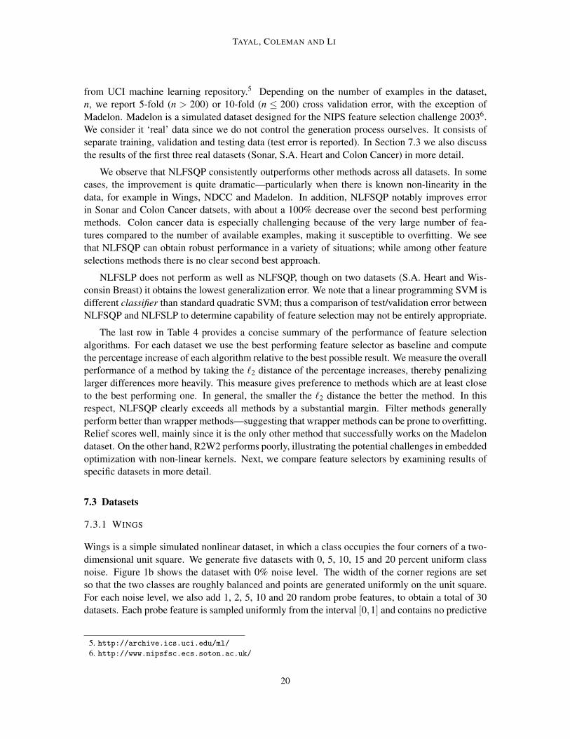
Figure 4: Subplots (a-e): Test error obtained on the 2-dimensional nonlinear Wings dataset withvarying degrees of uniform class noise. For each dataset we include additional probe fea-tures and compare the performance of different feature selection algorithms. With no classnoise most methods recover the base error rate, see subplot (a), but are not robust in thepresence of class noise, see subplot (b-e). The exception is NLFSQP, which consistentlyrecovers baseline error.

21


value. These datasets allow us to evaluate feature selection performance over different noise levelsand with varying density of useful features.

We use 200 training points, 200 tuning points and 1000 testing points for each dataset. Figures4a-e compare the test error obtained using different feature selection algorithms. We also includetest errors using no feature selection (labeled as NONE). The test error obtained when there are nonoise features (0 extra probes) and without any feature selection indicates the baseline error scoreachievable using SVM for each class noise level. We hope to recover the baseline error using featureselection as we increase the number of probe features.

For 0% class noise, Figure 4a, most feature selection methods are able to achieve the baselinetest error as number of probes are increased. The exceptions are R2W2 at 20 extra probes and L0with 2 or 5 extra probes. However, in the presence of class noise, Figure 4b-e, we see that filter andwrapper methods (MI, Relief, RFE and L0) fail when extra probe features are added. On occasion,Relief achieves baseline error: when there are 5 extra probes for 5% class noise, and 5 or 10 extraprobes for 10% class noise. Similarly, MI and RFE spuriously recover the correct features in the20% noisy dataset. Overall, we find results using filter and wrapper methods to be unreliable whenclass noise is present. In comparison, R2W2 performs fairly consistently across varying levels ofnoise; however, it fails when there are too many irrelevant features. This illustrates susceptibility tosuboptimal local minima in the embedded optimization problem. NLFSLP works effectively withmany irrelevant feature when class noise is low (0% or 5%), but for higher noise levels (10%, 15%and 20%), it fails when there are many probes (≥ 10). On the other hand, NLFSQP consistentlyrecovers baseline error, both as class noise and number of probe features are increased.

7.3.2 NDCC

Normally distributed clusters on cubes (NDCC) generates nonlinearly separable data by samplingfrom multivariate normal distributions with centers at the vertices of three concentric 1-norm cubes(Thompson, 2006). Each distribution uses a different (randomly generated) covariance matrix.Some centers generate a relatively small number of points, while others generate a relatively largenumber of points. Points at opposing vertices of each cube are assigned to opposite classes pre-venting linear separation. We create datasets to test feature selection by adding 2, 5, 10, 20, 50 and100 random probe features to a 20-dimensional NDCC dataset. Probe features are generated bysampling from a normal distribution.

Each dataset has 200 training points, 200 validation points, and 1000 testing points. Figure 5shows the test error obtained using different feature selection algorithms over increasing numberof probes. The baseline test error obtained using SVM when no probe features are used is 9.7%.We find that, without feature selec almost all modeling ability is lost with the addition of 5 extraprobes. Table 5 shows the number of correct features vis-a-vis total number of features identifiedby different feature selectors across the datasets.

Most feature selection algorithms successfully obtain the baseline error when there are only2 extra probes. Though MI and Relief do not identify all the correct features, the degradationin test error is minor. As we increase the number of probes, the performance of MI and Reliefprogressively deteriorates. RFE identifies the correct feature subset with up to 5 extra probes, butfails as additional probes are added. Similarly R2W2 fails when there are more than 10 extra probes.

22


0 2 5 10 20 50 1000.05

0.15

0.25

0.35

0.45

0.55T

est E

rror

Extra Probes

MI

RELIEF

RFE

L0

R2W2

NLFSLP

NLFSQP

NONE

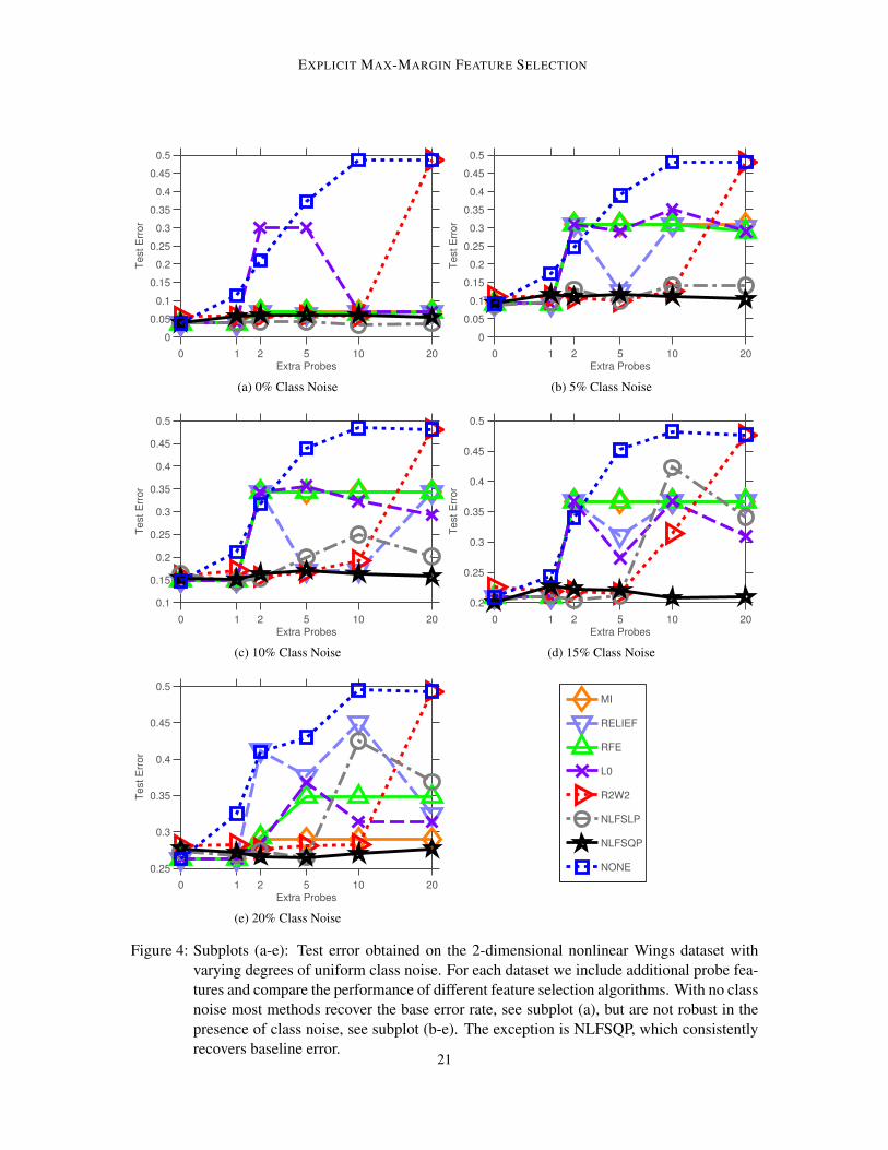
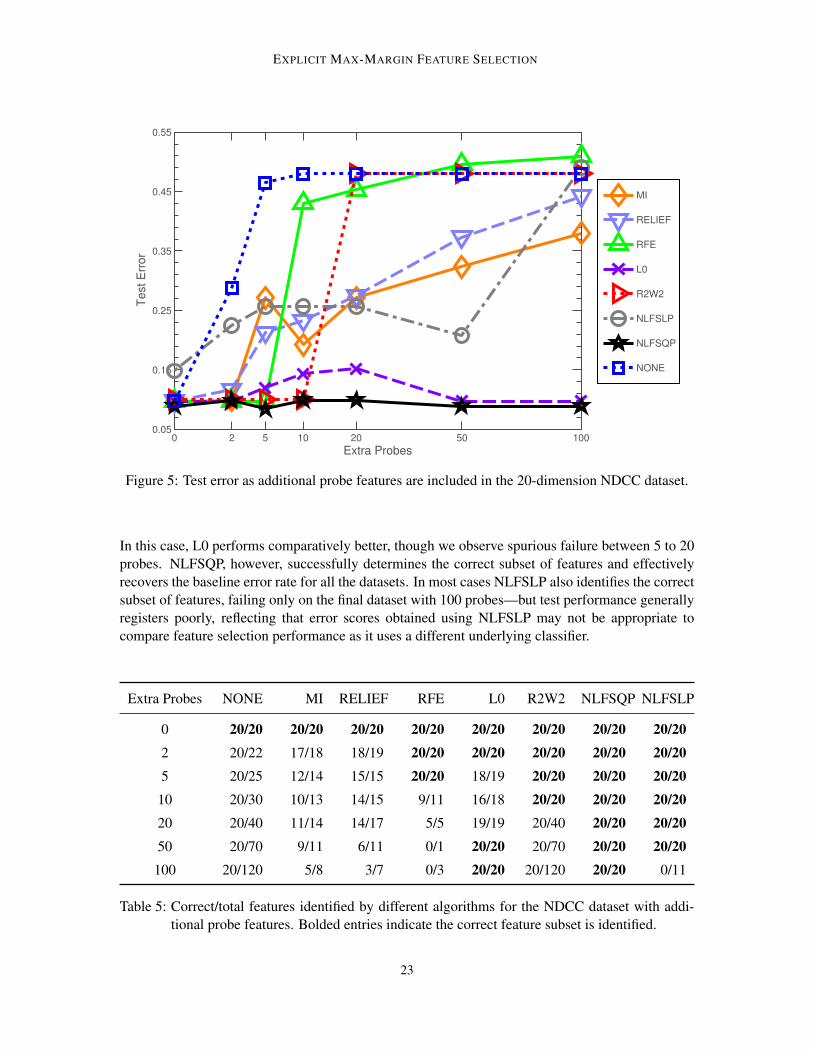
Figure 5: Test error as additional probe features are included in the 20-dimension NDCC dataset.

In this case, L0 performs comparatively better, though we observe spurious failure between 5 to 20probes. NLFSQP, however, successfully determines the correct subset of features and effectivelyrecovers the baseline error rate for all the datasets. In most cases NLFSLP also identifies the correctsubset of features, failing only on the final dataset with 100 probes—but test performance generallyregisters poorly, reflecting that error scores obtained using NLFSLP may not be appropriate tocompare feature selection performance as it uses a different underlying classifier.

Extra Probes NONE MI RELIEF RFE L0 R2W2 NLFSQP NLFSLP

0 20/20 20/20 20/20 20/20 20/20 20/20 20/20 20/202 20/22 17/18 18/19 20/20 20/20 20/20 20/20 20/205 20/25 12/14 15/15 20/20 18/19 20/20 20/20 20/2010 20/30 10/13 14/15 9/11 16/18 20/20 20/20 20/2020 20/40 11/14 14/17 5/5 19/19 20/40 20/20 20/2050 20/70 9/11 6/11 0/1 20/20 20/70 20/20 20/20100 20/120 5/8 3/7 0/3 20/20 20/120 20/20 0/11

Table 5: Correct/total features identified by different algorithms for the NDCC dataset with addi-tional probe features. Bolded entries indicate the correct feature subset is identified.

23


7.3.3 SONAR

Sonar is a popular dataset used to benchmark machine learning problems available from UCI repos-itory. The objective is to classify whether a sample is a rock or mine based on the energy responseof sonar signals. The dataset consists of 208 examples with 60 features. Figure 6 shows 5-fold crossvalidation results for different feature selection algorithms as a function of the number of featuresselected. Filter and wrapper methods provide a ranking of features, which is used to select features.For embedded methods we order features by the relative weight assigned to each feature. Resultsshown correspond to the optimal choice of C (and µ for NLFQP and NLFSLP) that yield minimumcross-validation error. We see that most methods use about 7-10 features and achieve a minimumerror between 15% and 20%. R2W2 obtains a slightly better score of 12% using 9 features, whileNLFSQP achieves the lowest error of 6.7% using 16 features. Note, feature weights obtained usingembedded methods may not necessarily reflect a ranking of feature importance, which possibly ex-plains why the error curve of NLFSQP falls above other methods when fewer features are selected.Moreover, this illustrates the importance of evaluating feature selection algorithms based on theirability to find the complete subset of relevant features. In this case, compared to NLFSQP all othermethods lead to suboptimal feature selection.

1 7 8 9 10 16 600

0.05

0.1

0.15

0.2

0.25

0.3

0.35

0.4

0.45

0.5

Cro

ss V

alidation E

rror

Number of Features Used

MI

RELIEF

RFE

L0

R2W2

NLFSLP

NLFSQP

NONE

Figure 6: Cross-validation error as a function of number of features used in the Sonar dataset. Forembedded methods a fixed set of non-zero feature weights are determined (used to orderfeatures), while the remainder of the features are not considered.

7.3.4 SOUTH AFRICAN HEART DISEASE

The South African heart disease data is a subset of the Coronary Risk-Factor Study survey carriedout in a heart-disease high-risk region of Western Cape, South Africa (Rossouw et al., 1983). The

24


data represents males between 15 and 64, and the response variable is the presence or absence ofmyocardial infraction. There are 160 cases and a sample of 302 controls. Each example consists ofnine risk factors which are potentially related to heart disease. The data is described in more detailin Hastie and Tibshirani (1987).

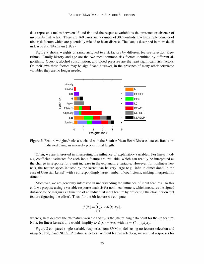
Figure 7 shows weights or ranks assigned to risk factors by different feature selection algo-rithms. Family history and age are the two most common risk factors identified by different al-gorithms. Obesity, alcohol consumption, and blood pressure are the least significant risk factors.On their own these factors may be significant, however, in the presence of many other correlatedvariables they are no longer needed.

0 1 2 3 4 5

famhist

age

adiposity

tobacco

typea

ldl

sbp

alcohol

obesity

Weight/Rank

Featu

re

MI

RELIEF

RFE

L0

R2W2

NLFSLP

NLFSQP

Figure 7: Feature weights/ranks associated with the South African Heart Disease dataset. Ranks areindicated using an inversely proportional length.

Often, we are interested in interpreting the influence of explanatory variables. For linear mod-els, coefficient estimates for each input feature are available, which can readily be interpreted asthe change in response for a unit increase in the explanatory variable. However, for nonlinear ker-nels, the feature space induced by the kernel can be very large (e.g. infinite dimensional in thecase of Gaussian kernel) with a correspondingly large number of coefficients, making interpretationdifficult.

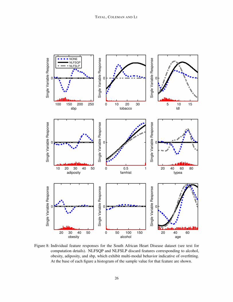
Moreover, we are generally interested in understanding the influence of input features. To thisend, we propose a single variable response analysis for nonlinear kernels, which measures the signeddistance to the margin as a function of an individual input feature by projecting the classifier on thatfeature (ignoring the offset). Thus, for the lth feature we compute

fl(xl) =n

∑j=1

y ju jK(xl,x jl),

where xl here denotes the lth feature variable and x jl is the jth training data point for the lth feature.Note, for linear kernels this would simplify to fl(xl) = wlxl with wl = ∑

nj=1 y ju jx jl .

Figure 8 compares single variable responses from SVM models using no feature selection andusing NLFSQP and NLFSLP feature selectors. Without feature selection, we see that responses for

25


100 150 200 250

0

sbp

Sin

gle

Va

ria

ble

Re

sp

on

se

NONE

NLFSQP

NLFSLP

0 10 20 30

0

tobacco

Sin

gle

Va

ria

ble

Re

sp

on

se

5 10 15

0

ldl

Sin

gle

Va

ria

ble

Re

sp

on

se

10 20 30 40 50

0

adiposity

Sin

gle

Va

ria

ble

Re

sp

on

se

0 0.5 1

0

famhist

Sin

gle

Va

ria

ble

Re

sp

on

se

20 40 60 80

0

typea

Sin

gle

Va

ria

ble

Re

sp

on

se

20 30 40 50

0

obesity

Sin

gle

Va

ria

ble

Re

sp

on

se

0 50 100 150

0

alcohol

Sin

gle

Va

ria

ble

Re

sp

on

se

20 40 60

0

age

Sin

gle

Va

ria

ble

Re

sp

on

se

Figure 8: Individual feature responses for the South African Heart Disease dataset (see text forcomputation details). NLFSQP and NLFSLP discard features corresponding to alcohol,obesity, adiposity, and sbp, which exhibit multi-modal behavior indicative of overfitting.At the base of each figure a histogram of the sample value for that feature are shown.

26


alcohol, obesity, adiposity, and sbp, are on average flat, but multi-modal, which suggest that themodel may be overfitting the data. Using NLFSQP or NLFSLP eliminates these features. In theprocess it also obtains more reasonable uni-modal responses for factors such as age, ldl, tobaccoand typea (note: NLFSQP and NLFSLP disagree on the relevance of tobacco and typea).

7.3.5 GENE MICROARRAY

Gene microarray data contains the expression of 2000 genes with highest minimal intensity across62 tissue samples, of which 40 are colon cancer cases and 22 are controls (Alon et al., 1999).Due to the large number of features in this dataset, here we use the subspace trust-region reflectivealgorithm and SR1 Hessian updates to speed up computation for NLFSQP and NLFSLP.

NLFSQP, Relief and MI are the best performing feature selectors for this dataset (refer to Table4). Table 6 lists the genes that each of these methods identify as being relevant for colon cancerdetection. Most of genes identified by MI are a subset of those identified by Relief, except Tag No.6814. NLFSQP selects a few of the same genes, but includes several others that are not chosen byRelief or MI.

Tag No. MI RELIEF NLFSQP Description

8147 X X X Human desmin gene, complete cds

692 X X Human cysteine-rich protein (CRP) gene, exons 5 and 6

37937 X X Myosin heavy chain, Nonmuscle (Gallus gallus)

9994 X X Hepatocyte growith factor–like protein precursor

43252 X Interferon-alpha receptor precursor (Homo sapiens)

36696 X Human mRNA for NCBP interacting protein 1

36689 X X H.sapiens mRNA for GCAP-II/uroguanylin precursor

12241 X Acetylcholine receptor protein, delta chain precursor

1207 X CALGIZZARIN

1812 X Homo sapiens macrophage capping protein mRNA

692 X X Human cysteine-rich protein (CRP) gene, exons 5 and 6

2344 X H.sapiens mRNA for hevin like protein

1832 X X Mysosin regulartory light chain 2, Smooth muscle isoform

12754 X Asialoglycoprotein receptor R2/3 (Rattus norvegicus)

44244 X Interleukin-1 receptor, Type II precursor (Homo sapiens)

6814 X Collagen alpha 2(XI) chain (Homo sapiens)

404 X Human MXI1 mRNA, complete cds

692 X Human cysteine-rich protein (CRP) gene, exons 5 and 6

1131 X Tropomysin, fibroblast and epithelial muscle-type (Human)

Table 6: Relevant genes identified by the top three performing feature selection methods for coloncancer detection.

27


Table 7 shows the number of genes used and their median absolute pair-wise correlations foreach method. Researchers are usually interested in identifying genes that are members of differentbiological pathways and consequently are less correlated. We see that NLFSQP identifies 11 genesthat have substantially lower correlation, whereas MI and Relief identify a set of genes that aremuch more correlated. Achieving a significantly lower cross-validation error with little correlationbetween genes indicates that NLFSQF is an effective non-linear multivariate feature selector evenin large dimensional spaces when only a small number of examples are available.

ALL MI RELIEF NLFSQP

No. of Genes 2000 6 10 11

Median absolute correlation 0.43 0.76 0.74 0.26

Table 7: Median absolute pair-wise correlations of gene expressions selected for colon-cancer de-tection. NLFSQP identifies genes which have less correlation indicating that they are mem-bers of different biological pathways.

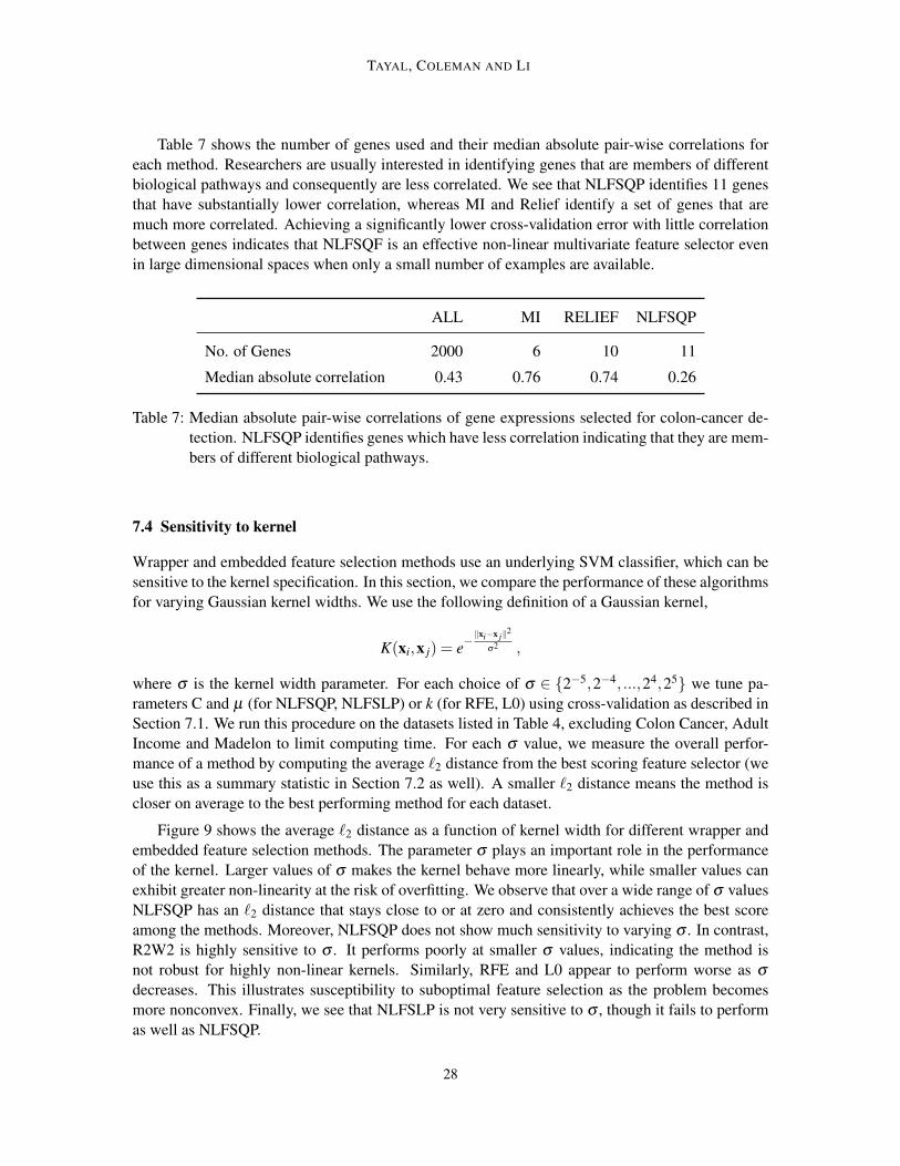
7.4 Sensitivity to kernel

Wrapper and embedded feature selection methods use an underlying SVM classifier, which can besensitive to the kernel specification. In this section, we compare the performance of these algorithmsfor varying Gaussian kernel widths. We use the following definition of a Gaussian kernel,

K(xi,x j) = e−‖xi−x j‖2

σ2 ,

where σ is the kernel width parameter. For each choice of σ ∈ 2−5,2−4, ...,24,25 we tune pa-rameters C and µ (for NLFSQP, NLFSLP) or k (for RFE, L0) using cross-validation as described inSection 7.1. We run this procedure on the datasets listed in Table 4, excluding Colon Cancer, AdultIncome and Madelon to limit computing time. For each σ value, we measure the overall perfor-mance of a method by computing the average `2 distance from the best scoring feature selector (weuse this as a summary statistic in Section 7.2 as well). A smaller `2 distance means the method iscloser on average to the best performing method for each dataset.

Figure 9 shows the average `2 distance as a function of kernel width for different wrapper andembedded feature selection methods. The parameter σ plays an important role in the performanceof the kernel. Larger values of σ makes the kernel behave more linearly, while smaller values canexhibit greater non-linearity at the risk of overfitting. We observe that over a wide range of σ valuesNLFSQP has an `2 distance that stays close to or at zero and consistently achieves the best scoreamong the methods. Moreover, NLFSQP does not show much sensitivity to varying σ . In contrast,R2W2 is highly sensitive to σ . It performs poorly at smaller σ values, indicating the method isnot robust for highly non-linear kernels. Similarly, RFE and L0 appear to perform worse as σ

decreases. This illustrates susceptibility to suboptimal feature selection as the problem becomesmore nonconvex. Finally, we see that NLFSLP is not very sensitive to σ , though it fails to performas well as NLFSQP.

28


−5 −4 −3 −2 −1 0 1 2 3 4 5

0

0.5

1

1.5

2

2.5

3

3.5

4

4.5

5

Gaussian kernel width (log2 σ)

Ave

rage

L2 f

rom

be

st sco

re

RFE

L0

R2W2

NLFSQP

NLFSLP

Figure 9: Sensitivity of wrapper and embedded feature selection performance to choice of Gaussiankernel width, σ . The y-axis measures the average `2 distance of percentage increases fromthe best scoring feature selector across eight datasets. NLFSQP consistently achieves thebest result for different σ values. NLFSLP is not sensitive to σ , although it does notperform as well as NLFSQP. Performance of R2W2, L0 and RFE degrades at small valuesof σ corresponding to highly curved decision surfaces.

7.5 Computational Efficiency

Generally, filter methods are computationally efficient and can scale to large datasets. However,in our cross validation scheme we learn and evaluate d SVMs to determine the optimal number offeatures, thus requiring O(d) SVM trainings. Similarly for wrapper methods, we require O(d) SVMtrainings as we eliminate features one by one. In the process we also determine the optimal numberof features via cross-validation. Thus we see that both filter and wrapper methods can be expensivein terms of the number of SVM trainings required for large d. This brute force approach can beimproved, for example, by eliminating or considering half-interval searches through the feature set,or using statistical methods to determine cutoff scores. However, this can result in reduced accuracy.In comparison, embedded methods can potentially use significantly fewer SVM training to identifythe relevant feature subset. Table 8 shows the number of trainings used by R2W2, NLFSQP andNLFSLP for different datasets. We observe that generally NLFSQP and NLFSLP use just a fewSVM trainings, and therefore can be efficient when number of data points, n, is large.

29


R2W2 NLFSQP NLFSLP

Wings (15%, +10) 84 5 4

NDCC (+20) 64 3 5

Sonar 78 3 3

S.A. Heart 94 4 5

Colon Cancer 91 7 16

Hepatitis 71 4 6

Wisconsin Breast 64 5 6

German Credit 71 6 4

Spambase 13 3 13

Adult Income 47 3 6

Madelon 57 5 4

Average no. of SVM runs 66.7 4.4 6.6

Table 8: Number of SVM trainings used by embedded feature selection methods on differentdatasets.

8. Conclusion

We have illustrated that feature selection for nonlinear SVMs can be challenging because of thenonconvexity inherent in the problem. As a result many local optima exist and it becomes NP hardto find the globally optimal subset of features. Heuristic filter and wrapper approaches have beenpopular because of their relative simplicity, however, they are prone to finding suboptimal featuresets, particularly when there are many irrelevant features or when class noise is present. Embed-ded SVM approaches offer greater potential since they can take into account complex nonlineardependencies tuned for the classifier. However, methods such as R2W2, for which only a first ordergradient descent method is readily applicable, can be susceptible to suboptimal solutions as well.

In this paper, we presented an embedded feature selection method based on the primal nonlinearSVM. We solve this nonconvex minimization problem using a second-order trust region method,which explicitly exploits the negative curvature of the objective function to increase the possibilityof reaching global minimum. For computational efficiency, we apply an alternating optimizationframework (NLFSQP). In addition, we illustrate that a naive application of AO can lead to iteratesbeing trapped at saddle points. Using a perspective mapping, we extend the space in which AO isperformed. In order to achieve better feature selection, we further relax the normalization constraintin the feature selection subproblem and propose an explicit margin maximization feature selectionframework.

Our results (see Table 4) indicate that NLFSQP consistently outperforms other methods on avariety of datasets. Moreover, we illustrate that for highly nonlinear kernels, NLFSQP continues tobe effective, whereas most methods perform poorly (see Figure 9). We believe that there are three

30


main contributing factors for the success of NLFSQP: (a) the use of an explicit margin when workingwithin an alternating optimization framework, to reduce saddle point and suboptimal convergence,(b) exploiting second-order curvature information, and (c) the use of bound constrained trust regionalgorithm, which provides robust global convergence.

In addition, we have also applied the explicit max-margin technique to 1-norm linear program-ming SVMs (NLFSLP). In general, NLFSLP did not perform as well as NLFSQP in terms ofgeneralization error. This is partly because it uses a structurally different classifier and thereforegeneralization error is not directly comparable to standard quadratic programming SVMs (e.g. seeTable 5 which shows NLFSLP identifies correct features but is unable to produce a competitive gen-eralization error). However, NLFSLP performs well compared to other methods, particularly whenusing highly nonlinear kernels (Figure 9).

Often, choosing an appropriate nonlinear feature selection method is a trial and error process,due to the inherent nonconvexity in the problem. We believe that our new NLFSQP approach is animportant step towards a robust approach, using second order trust region optimization to effectivelytackle nonconvexity. Subsequently, we hope to explore a very large scale implementation, whichdoes not require storing the Hessian matrix and can take advantage of feature sparsity, to solveproblems with hundreds of thousands to millions of features.

References

U. Alon, N. Barkai, D. A. Notterman, K. Gish, S. Ybarra, D. Mack, and A. J. Levine. Broad patternsof gene expression revealed by clustering analysis of tumor and normal colon tissues probed byoligonucleotide arrays. Proceedings of the National Academy of Sciences of the United States ofAmerica, 96(12):6745–6750, 1999.

J. C. Bezdek and R. J. Hathaway. Some notes on alternating optimization. In Proceedings of the2002 AFSS International Conference on Fuzzy Systems (AFSS ’02), pages 288–300, 2002.

B. E. Boser, I. M. Guyon, and V. N. Vapnik. A training algorithm for optimal margin classifiers.In Proceedings of the fifth annual workshop on Computational learning theory, COLT ’92, pages144–152. ACM, 1992.

S. Boyd and L. Vandenberghe. Convex Optimization. Cambridge University Press, 2004.

P. S. Bradley and O. L. Mangasarian. Feature selection via concave minimization and support vectormachines. In Machine Learning Proceedings of the Fifteenth International Conference(ICML98), pages 82–90, 1998.

M. A. Branch, T. F. Coleman, and Y. Li. A subspace, interior, and conjugate gradient methodfor large-scale bound-constrained minimization problems. SIAM J. Scientific Computing, 21(1):1–23, 1999.

H. Byun and S.-W. Lee. Applications of support vector machines for pattern recognition: A survey.In Pattern Recognition with Support Vector Machines, pages 213–236. 2002.

31


A. B. Chan, N. Vasconcelos, and G. R. G. Lanckriet. Direct convex relaxations of sparse svm. InProceedings of the 24th international conference on Machine learning, ICML ’07, pages 145–153. ACM, 2007.

O. Chapelle. Training a support vector machine in the primal. Neural Comput., 19(5):1155–1178,2007.

T. F. Coleman and Y. Li. An interior trust region approach for nonlinear minimization subject tobounds. SIAM Journal on Optimization, 6(2):415–425, 1996.

C. Cortes and V. Vapnik. Support-vector networks. Machine Learning, 20(3):273–297, 1995.

R. Courant and D. Hilbert. Methods of Mathematical Physics. Interscience, 1953.

R.-E. Fan, P.-H. Chen, and C.-J. Lin. Working set selection using second order information fortraining support vector machines. Journal of Machine Learning Research, 6:1889–1918, 2005.

G. M. Fung and O. L. Mangasarian. A feature selection newton method for support vector machineclassification. Computational Optimization and Applications, 28(2):185–202, 2004.

L. Grippo and M. Sciandrone. On the convergence of the block nonlinear Gauss-Seidel methodunder convex constraints. Operations Research Letters, 26:127–136, 2000.

I. Guyon and A. Elisseeff. An introduction to variable and feature selection. Journal of MachineLearning Research, 3:1157–1182, 2003.

I. Guyon, J. Weston, S. Barnhill, and V. Vapnik. Gene selection for cancer classification usingsupport vector machines. Machine Learning, 46(1-3):389–422, 2002.

I. Guyon, H. M. Bitter, Z. Ahmed, M. Brown, and J. Heller. Multivariate nonlinear feature selectionwith kernel multiplicative updates and gram-schmidt relief. 2003 BISC FLINT-CIBI workshop,2003.

T. Hastie and R. Tibshirani. Nonparameteric logistic and proportional odds regression. AppliedStatistics, 36:270–276, 1987.

K. Kira and L. Rendell. A practical approach to feature selection. In ML92: Proceedings of theninth international workshop on Machine learning, pages 249–256, 1992.

O. L. Mangasarian and G. Kou. Feature selection for nonlinear kernel support vector machines.Seventh IEEE International Conference on Data Mining Workshops ICDMW 2007, pages 231–236, 2007.

E. Marchiori. Feature selection for classification with proteomic data of mixed quality. In InProceedings of the 2005 IEEE Symposium on Computational Intelligence in Bioinformatics andComputational Biology, pages 385–391, 2005.

J. Mercer. Functions of positive and negative type and their connection with the theory of integralequations. Philos. Trans. Royal Soc. (A), 83(559):69–70, 1909.

32


X. Nguyen, M. J. Wainwright, and M. I. Jordan. On surrogate loss functions and f-divergences.Annals of Statistics, 37(2):876–904, 2009.

J. Nocedal and S. J. Wright. Numerical Optimization. Springer, 2000.

J. C. Platt. Advances in kernel methods. chapter Fast training of support vector machines usingsequential minimal optimization, pages 185–208. MIT Press, 1999.

M. Rojas, S. Santos, and D. Sorensen. Algorithm873:LSTRS: Matlab software for large-scale trustregion subproblems and regularization. ACM Transaction on Mathematical Software, 34(2):11,2008.

S. Rosset, J. Zhu, and T. Hastie. Margin maximizing loss functions. In Advances in Neural Infor-mation Processing Systems (NIPS 15). MIT Press, 2003.

J. E. Rossouw, J. P. Du Plessis, A. J. Benade, P. C. Jordaan, J. P. Kotze, P. L. Jooste, and J. J.Ferreira. Coronary risk factor screening in three rural communities. the CORIS baseline study.South African Medical Journal, 64(12):430–6, 1983.

B. Scholkopf and A. J. Smola. Learning with Kernels. MIT Press, 2002.

B. Scholkopf, K. Tsuda, and J. P. Vert, editors. Kernel Methods in Computational Biology. MITPress, 2004.

M. Tan, L. Wang, and I. W. Tsang. Learning sparse svm for feature selection on very high di-mensional datasets. In Proceedings of the 27th International Conference on Machine Learning(ICML-10), pages 1047–1054, 2010.

M. E. Thompson. NDCC: normally distributed clustered datasets on cubes, 2006.www.cs.wisc.edu/dmi/svm/ndcc/.

R. Tibshirani. Regression shrinkage and selection via the lasso. J. Roy. Statist. Soc. Ser. B, 58(1):267–288, 1996.

V. N. Vapnik. Statistical Learning Theory. Wiley, 1st edition, 1998.

M. R. Sikonja and I. Kononenko. Theoretical and empirical analysis of ReliefF and RReliefF.Machine Learning, 53(1-2):23–69, 2003.

J. Weston, S. Mukherjee, O. Chapelle, M. Pontil, and V. Vapnik. Feature selection for SVMs. InAdvances in Neural Information Processing Systems 13, volume 13, pages 668–674, 2000.

J. Weston, A. Elisseeff, B. Scholkopf, and M. Tipping. Use of the zero norm with linear models andkernel methods. Journal of Machine Learning Research, 3:1439–1461, 2003.

Y. X. Yuan. A review of trust region algorithms for optimization. In ICM99: Proc. 4th Int. Congresson Industrial and Applied Mathematics, pages 271–282. Oxford University Press, 2000.

M. Zaffalon and M. Hutter. Robust feature selection by mutual information distributions. In Pro-ceedings of the Eighteenth conference on Uncertainty in artificial intelligence, UAI’02, pages577–584, 2002.

33


W. Zhou. Linear programming support vector machines. Pattern Recognition, 35(12):2927–2936,2002.

J. Zhu, S. Rosset, T. Hastie, and R. Tibshirani. 1-norm support vector machines. In Neural Infor-mation Processing Systems, volume 16, 2003.

34

explicit max margin input feature selection for nonlinear svm …tfcolema/articles/fspaper.pdf ·...

Documents