a new hysteretic reactor model for transformer energization applications title: by : afshin...
TRANSCRIPT

A New Hysteretic Reactor Model for A New Hysteretic Reactor Model for
Transformer Energization Transformer Energization ApplicationsApplications
Title:
By:
Afshin Rezaei-Zare & Reza Iravani
University of Toronto
June 2011

OutlineOutline
1. Existing hysteresis models in EMT programs
2. Drawbacks of the existing models
3. New hysteretic reactor model
4. Impact on Remnant Flux (Lab. Measurement)
5. De-energization / Re-energization
6. 33kV-VT Ferroresonance Lab. test results
7. Conclusions
8. Applications

• EMTP Type-96
• EMTP Type-92 (Current Hysteresis model of the EMTP-RV)
• PSCAD/EMTDC Jiles-Atherton model (Not a reactor but incorporated in the CT model)
• Proposed New Hysteretic Reactor
Existing Hysteresis Models Existing Hysteresis Models in EMT Programsin EMT Programs

Type 96 modelType 96 model
Piecewise linear modelPiecewise linear model
Originally developed by Talukdar and Bailey in Originally developed by Talukdar and Bailey in 1976 and modified in 1982 by Frame and 1976 and modified in 1982 by Frame and MohanMohan
Simple and computationally efficientSimple and computationally efficient
Minor loops are obtained by linearly Minor loops are obtained by linearly decreasing the distance between the reversal decreasing the distance between the reversal point and the penultimate reversal pointpoint and the penultimate reversal point

Drawbacks of Type 96 ModelDrawbacks of Type 96 Model
No stack is used to store the extrema of excitation which leads to open cycles
Similarity of minor loops to the major loop due to scaling approach used by the model (such a similarity is not valid in reality)
The existence of a saturation point is not verified experimentally
The model implemented in EMTP-V3 is pseudo nonlinear
Drawbacks of Type 96 Model – Drawbacks of Type 96 Model – Cont’dCont’d
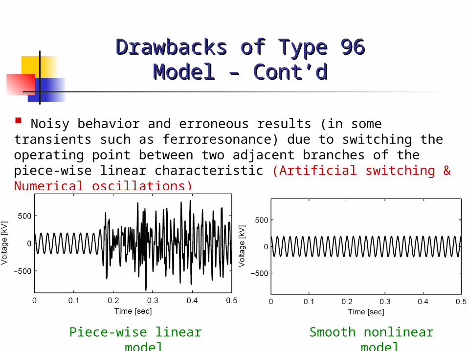
Noisy behavior and erroneous results (in some transients such as ferroresonance) due to switching the operating point between two adjacent branches of the piece-wise linear characteristic (Artificial switching & Numerical oscillations)
Piece-wise linear model
Smooth nonlinear model

Type 92 modelType 92 model
Developed in 1996 by Ontario HydroDeveloped in 1996 by Ontario Hydro
Based on hyperbolic functionsBased on hyperbolic functions
Instantaneous flux is separated in two Instantaneous flux is separated in two components: components: i) hysteresis (irreversible) i) hysteresis (irreversible) ii) saturation (reversible) ii) saturation (reversible)
Current EMTP-RV model is based on this Current EMTP-RV model is based on this approachapproach

Hyperbolic functions in Type 92: Hyperbolic functions in Type 92: instantaneous flux is used to find unsaturated flux instantaneous flux is used to find unsaturated flux which is then used to find instantaneous currentwhich is then used to find instantaneous current
Model Type 92Model Type 92
slope
slope
Saturated flux vs. Unsaturated flux (to describe saturation)
Unsaturated flux vs. Current (to describe hysteresis)

Drawbacks of Type 92 ModelDrawbacks of Type 92 Model
Raw dataFitted data
Inaccuracy (1)Inaccuracy (1)
Limited flexibility to fit to the hysteresis major loop (only based on one hyperbolic term)

Drawbacks of Type 92 ModelDrawbacks of Type 92 Model
Inaccuracy (2)Inaccuracy (2)
Only upper part of the trajectory is used and the lower part is assumed to be symmetric to the upper part (while in reality the shapes of the two parts are independent)
-30 -20 -10 0 10 20 30-600
-400
-200
0
200
400
600
Courant(A)
Flu
x(W
b)
IC
Current (A)

Jiles-Atherton ModelJiles-Atherton Model
Physically correct model
decomposes the magnetization into “reversible anhysteretic” and “irreversible” components based on a weighted average:
Reversible part is based on Langevin function:
Irreversible part is based on the differential equation:

Drawbacks of the Jiles-Atherton Drawbacks of the Jiles-Atherton ModelModel
Limited flexibility to fit to the measurements due to the utilized Langevin function, and the model very few parameters (5 parameters)
In some cases, non-physical results as the input current changes the direction
Formations of minor loops and the major loop are dependent (changing the parameters changes both minor and major loop shapes)
In the PSCAD/EMTDC, it is not available as a reactor to build a desired general system for transient studies.(Only incorporated in a CT model)

New Hysteretic Reactor ModelNew Hysteretic Reactor Model
• A modified Preisach Model - a time-domain implementation with true-nonlinear solution within the EMTP-RV - Independent formation of minor loops from the major loop (consistent with the observed hysteresis loops of the magnetic materials)
• Physically correct hysteresis model
• Memory dependent model: past excitation extrema are stored in memory to form the magnetization trajectories.
• Representing wiping-out property, (a well-known physical property of the ferromagnetic materials)

New Hysteretic Reactor ModelNew Hysteretic Reactor Model
-1.5 -1 -0.5 0 0.5 1 1.5
-1.5
-1
-0.5
0
0.5
1
1.5
Magnetizing Current [A]
Flu
x L
inka
ge
[V.s
]
Major loopMagnetizationTrajectory
-1.5 -1 -0.5 0 0.5 1 1.5
-1.5
-1
-0.5
0
0.5
1
1.5
Magnetizing Current [A]
Flu
x L
inka
ge
[V.s
]
))_(tanh()(
)(sech)tanh()(
)(*,
1
2
shiftxxpDCxMinor
xcxBxMajor
xMinorxMajorxFn
iiiii
Same major loops – Different minor Same major loops – Different minor loopsloops
Forms major Forms major looploop
Forms minor Forms minor looploop

New Hysteretic Reactor ModelNew Hysteretic Reactor Model
+ Am1
?i
VM+m2
?v
+R1
60
+
AC1
20kVRMS /_0
scope Voltage
scope Fulx
scope Current
scope L
Pic
60Hz
p1
scopeHys_Power
Current
Flux
L
Voltage+
P
DEV1

New Hysteretic Reactor New Hysteretic Reactor ModelModel

Hysteresis Shapes
-5 -4 -3 -2 -1 0 1 2 3 4 5
-80
-60
-40
-20
0
20
40
60
80
Current@control@1
y
PLOT
-5 -4 -3 -2 -1 0 1 2 3 4 5-100
-80
-60
-40
-20
0
20
40
60
80
100
Current@control@1
y
PLOT
-0.6 -0.4 -0.2 0 0.2 0.4 0.6
-80
-60
-40
-20
0
20
40
60
80
100
Current@control@1
yPLOT
-5 -4 -3 -2 -1 0 1 2 3 4 5-100
-80
-60
-40
-20
0
20
40
60
80
100
Current@control@1y
PLOT
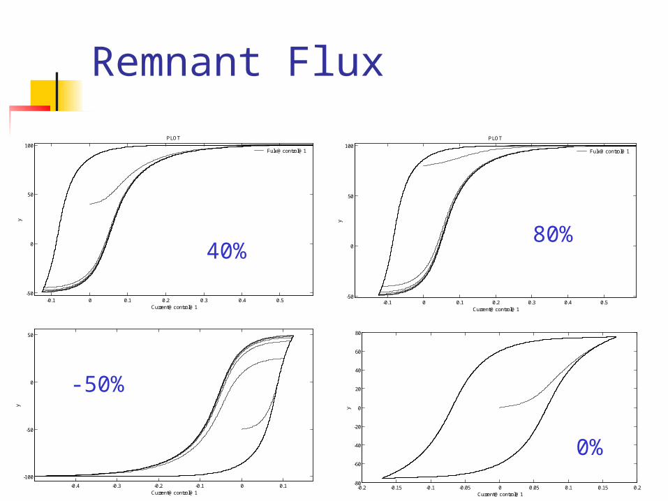
Remnant Flux
-0.4 -0.3 -0.2 -0.1 0 0.1
-100
-50
0
50
Current@control@1
y
PLOT
-0.1 0 0.1 0.2 0.3 0.4 0.5-50
0
50
100
Current@control@1
y
PLOT
Fulx@control@1
-0.2 -0.15 -0.1 -0.05 0 0.05 0.1 0.15 0.2-80
-60
-40
-20
0
20
40
60
80
Current@control@1
y
PLOT
-0.1 0 0.1 0.2 0.3 0.4 0.5-50
0
50
100
Current@control@1
y
PLOT
Fulx@control@1
40%80%
-50%
0%

Harmonic Initialization
60 Hz
180 Hz
300 Hz
420 Hz
0 Hz
+ Am1
?i
VM+m2
?v
+R1
30
+
AC1
25kVRMS /_0
+R2
30
+R3
30
+
AC3
40kVRMS /_135
+R4
30
+
AC4
40kVRMS /_30
+L1
80mH
+
C2
300nF
+
AC2
60kVRMS /_30
+R5
2k
1
DC1
scope Voltage
scope Fluxscope Current
scope L
+
P
DEV1
CurrentFluxLVoltage
-0.005 0 0.005 0.01 0.015 0.02 0.025 0.03 0.035-40
-20
0
20
40
60
80
100
120
Current@control@1
yPLOT

Impact on Remnant Flux (Lab. Measurement)
40 50 60 70 80 90 100
-1
0
1
2
3
4
5
6
Ma
gn
tizin
g C
urr
en
t*1
0 [A
]
seco
nd
ary
vo
ltag
e [V
]
Time [ms]
im
VS
0 10 20 30 40 50 60 70 80 90 100
0
0.5
1
1.5
2
Co
re M
ag
ne
tizin
g C
urr
en
t [A
]
Time [ms]
Close-up Window
im
VS
imIron Core

Impact on Remnant Flux (Lab. Measurement) – Cont’d
0 0.5 1.0 1.5 2.0
-0.01
0
0.01
0.02
0.03
0.04
0.05
0.06
0.07
0.08
0.09
Magnetizing Current [A]
Flu
x [V
.s]
Major loopMeasured trajectory
-150 -100 -50 0 50-0.01
-0.005
0
0.005
0.01
0.015
0.02
Magnetizing Current [mA]
Flu
x [V
.s]
Major loopMeasurementEMTP Type-96New Reactor

De-energization / Re-De-energization / Re-energizationenergization
0 0.2 0.4 0.6 0.8 1 1.2 1.4 1.6 1.8 2-30
-20
-10
0
10
20
30
40
Time [sec]
Fa
ult
Cu
rre
nt [
kA]
0.6 sec 1.0 sec
Auto-reclosure operations on a 12kA Fault Auto-reclosure operations on a 12kA Fault Current Current

-1.5 -1 -0.5 0 0.5 1 1.5
-1.5
-1
-0.5
0
0.5
1
1.5
Magnetizing Current [A]
Flu
x L
inka
ge
[V.s
]
Remnant Flux subsequent to the
second current interruption
-1.5 -1 -0.5 0 0.5 1 1.5
-1.5
-1
-0.5
0
0.5
1
1.5
Magnetizing Current [A]
Flu
x L
inka
ge
[V.s
]
-1.5 -1 -0.5 0 0.5 1 1.5
-1.5
-1
-0.5
0
0.5
1
1.5
Magnetizing Current [A]
Flu
x L
inka
ge
[V.s
]
Major loopMagnetizationTrajectory
Different Minor loop shapes
Different Remnant Flux
(for the same switching scenario)
Remnant flux

1.79 1.8 1.81 1.82 1.83 1.84 1.85 1.86
-50
0
50
100
Time [sec]
Se
con
da
ry C
urr
en
t [A
]
1.79 1.8 1.81 1.82 1.83 1.84 1.85 1.86
-50
0
50
100
Time [sec]
Se
con
da
ry C
urr
en
t [A
]
1.79 1.8 1.81 1.82 1.83 1.84 1.85 1.86
-50
0
50
100
Time [sec]
Se
con
da
ry C
urr
en
t [A
]
Impacts on CT Saturation and Impacts on CT Saturation and protectionprotection
(Following the final reclosure on the permanent fault)(Following the final reclosure on the permanent fault)

0 10 20 30 40 50 60 70 80
-60
-40
-20
0
20
40
60
Time [sec]
Vo
ltag
e [k
V]
30.7 kV (1.14pu)
63.5 kV (2.36pu)
52.4 kV (1.94pu)
38.4 kV (1.43pu)
11.8 kV (0.44pu)
33kV-VT Ferroresonance Laboratory test results
Source peak voltage
Measured VT voltage

10 30 50 70 90 110 130 150 170 190 210 230
-60
-40
-20
0
20
40
60
Time [ms]
Vo
ltag
e [k
V]
33kV-VT Ferroresonance Lab Test
52.4 kV (1.94pu)
63.5 kV (2.36pu)
0
50
100
150
200
250
Pm
[W]
103 W
29 W
Power Loss
Voltage
218 W

33kV-VT Ferroresonance Lab Test
Model Type-92
Hysteresis Loop
-10 0 10 20 30 40 50 60-20
0
20
40
60
80
100
120
140
160
180
Magnetizing Current [mA]
Co
re F
lux
[V.s
]
EMTP-RVFitted Hysteresis LoopTest data
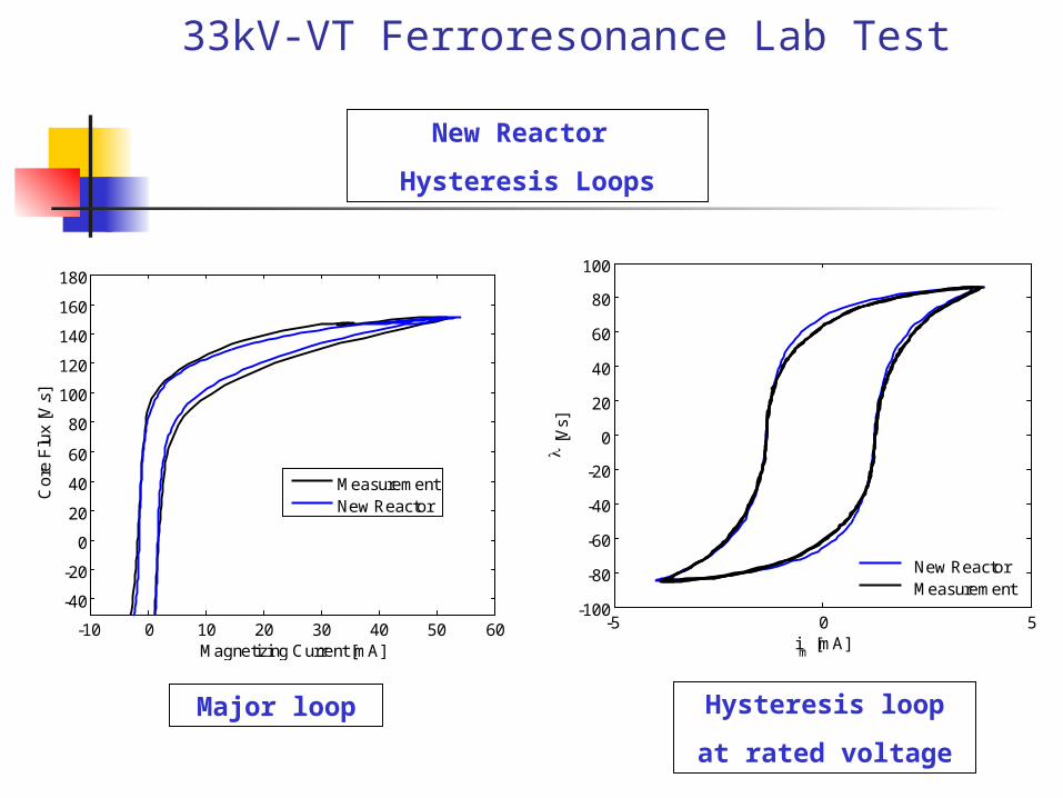
33kV-VT Ferroresonance Lab Test
Major loop
-5 0 5-100
-80
-60
-40
-20
0
20
40
60
80
100
im
[mA]
[V
s]
New Reactor Measurement
Hysteresis loop
at rated voltage
New Reactor
Hysteresis Loops
-10 0 10 20 30 40 50 60
-40
-20
0
20
40
60
80
100
120
140
160
180
Magnetizing Current [mA]
Co
re F
lux
[V.s
]
MeasurementNew Reactor

33kV-VT Ferroresonance Lab Test
Bifurcation Points
24 25 26 27 28 29 30 31 3220
25
30
35
40
45
50
55
60
65
70
VT
Pe
ak
Vo
ltag
e [k
V]
Source Peak Voltage [kV]
EMTPType-96
HystereticModel
Single-valuedSaturation
Model
New ReactorModel MeasurementEMTP-RV
HystereticModel

33kV-VT Ferroresonance Lab TestCore Power Loss
20
40
60
80
100
120
140
160
180
200
220
Po
we
r L
oss
[W]
MeasurementEMTP Type-96
20
40
60
80
100
120
140
160
180
200
220
Po
we
r L
oss
[W]
MeasurementEMTP-RV
0 50 100 150 20020
40
60
80
100
120
140
160
180
200
220
Time [ms]
Po
we
r L
oss
[W]
MeasurementNew Reactor
Power Loss
Comparison

33kV-VT Ferroresonance Lab Test – Cont’dHysteresis Loops Comparison
-8 -6 -4 -2 0 2 4 6 8
-100
-80
-60
-40
-20
0
20
40
60
80
100
Magnetizing Current [mA]
Co
re F
lux
[V.s
]
-8 -6 -4 -2 0 2 4 6 8
-100
-80
-60
-40
-20
0
20
40
60
80
100
Magnetizing Current [mA]
Co
re F
lux
[V.s
]
-8 -6 -4 -2 0 2 4 6 8
-100
-80
-60
-40
-20
0
20
40
60
80
100
Magnetizing Current [mA]
Co
re F
lux
[V.s
]
-8 -6 -4 -2 0 2 4 6 8 10
-100
-80
-60
-40
-20
0
20
40
60
80
100
Magnetizing Current [mA]
Co
re F
lux
[V.s
]
Measurement
EMTP-RV
(Type 92)
EMTP
Type-96
New
Reactor

33kV-VT Ferroresonance Lab Test
Dynamic Inductance
( Slope of magnetization trajectories )
Before Ferroresonance
(Normal conditions)
Under Ferroresonance
conditions
-100 -50 0 50 1000
50
100
150
200
250
Core Flux [V.s]
LD
yn [k
H]
-150 -100 -50 0 50 100 1500
20
40
60
80
100
120
140
160
180
Core Flux [V.s]
LD
yn [k
H]
New ReactorMeasurementSingle-Valuedsaturation modelEMTP Type-96EMTP-RV model

Capability of the models to represent the core dynamic behaviors
Core Inductance change
As the core is driven into ferroresonance with respect to normal operation
Change directionModel
Measurement
New Reactor
EMTP Type-96
EMTP-RV (Type-92)
Single-valued saturation curve
No change
No change
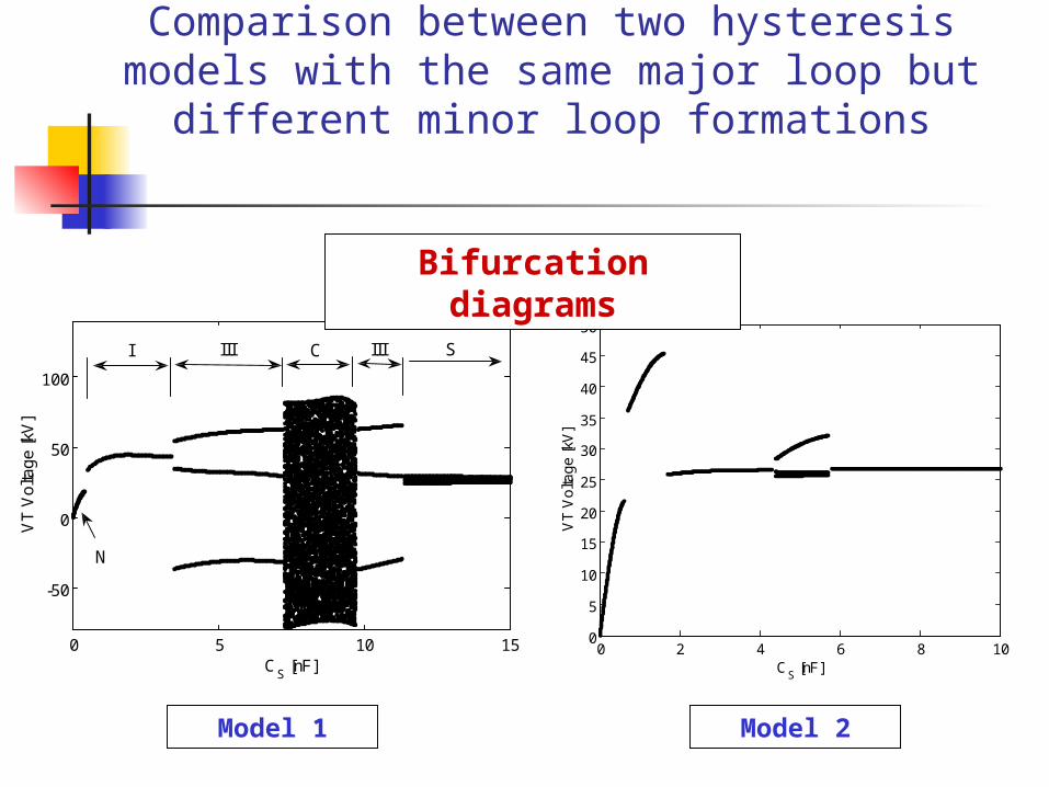
Another Example – Comparison between two hysteresis models with the same major loop but different minor
loop formations
Model 1
0 5 10 15
-50
0
50
100
CS [nF]
VT
Vo
ltag
e [k
V]
I III C III S
N
0 2 4 6 8 100
5
10
15
20
25
30
35
40
45
50
CS [nF]
VT
Vo
ltag
e [k
V]
Model 2
Bifurcation diagrams

Ferroresonance demo
Disconnect Silver Charge at T=50 ms
Disconnect Silver Charge at t=50 ms Trip line at T=80 ms and Rf at T=100ms
Data Case given to us by David Jacobson. See also:Jacobson D. A. N., Marti, L., Menzies, R.W., "Modeling Ferroresonance in a 230 kVTransformer-Terminated Double-Circuit Transmission Line"Proceedings of the 1999 International Conf. on Power systems Transientspp. 451-456, June 20-24, Budapest
Trip line AR3 at t=80 ms
+
VERMILLION
184.629622kV /_79.0299
+
+R_ASROS
+ DORSEY
193.198699kV /_84.5124
+
RIDGEWAY
203.690636kV /_73.5250
+
ROSSER
204.937080kV /_76.3223
+
+
+
+
R_ROSAS
+
C_DORAS
+S_ROSAS
+
129.71
A6V
+ D13R_D16R
19.46
+
C_ASROS
+
C_ASDOR
+
C_SILCT
+R_SILCT
+
C_SIL2H
+R_SIL2H
+
1214/285.6Ohm
CHARGE_SILVER
+
C_SILVS
+
C_SILVH
+
C_SIL2H
+
C_SIL2S
+
A3R_1_SILVB
Current
Transformer
CT
+
RL1
8/6.937Ohm
+
CHARGE_GRAPD
+
CHARGE_ASHERN
+R_SILVL
1E12+
R_ROSDU
+Z
nO ZnO1
?vip
>e
516kV
+
0.01
VM+
ASDOR
VM+
ASROS
1 2
DYg_1
13.8/230
+
S_ASG1A
+
S_ASG2A
+
S_ASVER
+
S_ASROS_ASRMA
+S_ASDOR_ASRMA
+S_SILVL
+S_SIL2H
+S_SILCT
+S_ROSDU
+
S_A3R_1
+
S_SCITS
+
S_GRVER
+
S_DORRI
+
DOR13
+
DOR16
+DOR5R
+S_DORAS
+
S_ASROS
+
S_ASDOR
VM+
ASHERN
VM+
ROSSR
VM+
ROSAS
VM+
A4D07
VM+
DORB2A
VM+
SILVHVM+
SILVS
VM+ SILVB
+
part
+ D5R
19.46
+
D36R_R23R
16.41
+C_ROSAS
+
C_ROSIL
+
S_ROSIL
+
S_SILRO+
ROSSER_SILVER
95
+
234.35
G1A_G2A
+
S_GRG1?i
+
G31V
+
S_GRG2?i
VM+
GRAPD
VM+
A3R02
AR3
A4D transmission_lines
3-Phases
BCTRANTransformer
&Hysteresis
TRANSFO2
SILVER_230_66
HAHBHCSC
SASB
3-Phases
BCTRANTransformer
&HysteresisTRANSFO1
SILVER_230_66
DampingReactor
ASRMAASM
GRAND_RAPIDS
?m
13.8kV460MVA
scopeZno_energy_a
scopeZno_energy_b
scopeZno_energy_c
cba
VERM
cba
DORASA
c
ba
A3R_1
cba
bac
SIL2S
abc
SILVH
cba
SILVS
abc
ASROS
abc
ASDOR
cba
ASG1A
cba
ASG2A
SILVL
bc
a
SIL2H
SILCT
cba
SILVB
abc
ROSAS
abc
BUS2
c b a
cba
DORRI
cba
DORB2
ASHERN
a
a
b
b
c
c
A4D07
A3R02
D36c
D36c
D36b
D36b
D36a
D36a
c
c
b
b
aa
BUS4
c
cc
c
a
a
a
a
b
b
b
b
ROSSR
GRG1
abc
GRAPD
GRG2
cba
e_ZnO1a
e_ZnO1b
e_ZnO1c

Ferroresonance demo
Conclusions
• The model is based on widely-verified and accepted Preisach model of hysteresis
• Independent formation of major and minor loops
• True nonlinear solution within the EMTP-RV
• Can accurately represent the physical properties of the magnetic core materials
• Can accurately represent the dynamic core behavior under electromagnetic transients
New Model Features

Applications
For accurate EMTP studies on :
De-energizing/re-energizing of transformers
Ferroresonance phenomena in power and instrument transformers
Determination of the core remnant flux
Precise modeling of VTs, CTs, and CVTs for protection studies
Accurate modeling of electrical machines
Efficient design of control systems for power-electronic based drives by taking into account the machine nonlinearity and actual power loss
Important points
• It is evident that a more detailed model needs more parameters. although, a model with simple implementation and with less required parameters is generally preferable, the accuracy of such models are limited.
• For a sophisticated hysteresis model, “not needing minor loop data”, is a drawback not an advantage. Due to different behavior of minor loops (extensively verified by experiments), neglecting the minor loop parameters can result in completely different and unexpected results.
• For the new reactor, if the minor loop data are not available, a set of pre-specified default values can be considered.