a new forecasting model for usd/cny exchange rate

Studies in Nonlinear Dynamics &Econometrics

Volume 16, Issue 3 2012 Article 4

A New Forecasting Model for USD/CNYExchange Rate

Zongwu Cai∗ Linna Chen†

Ying Fang‡

∗University of North Carolina at Charlotte, [email protected]†Xiamen University, [email protected]‡Xiamen University, [email protected]

DOI: 10.1515/1558-3708.1878

Copyright c©2012 De Gruyter. All rights reserved.

A New Forecasting Model for USD/CNYExchange Rate∗

Zongwu Cai, Linna Chen, and Ying Fang

Abstract

This paper models the return series of USD/CNY exchange rate by considering the conditionalmean and conditional volatility simultaneously. An index type functional-coefficient model isadopted to model the conditional mean part and a GARCH type model with a policy dummyvariable is applied to the conditional volatility model. We show that the government policy indeedhas an impact on the exchange rate dynamic. To evaluate the out-of-sample forecasting ability, aprediction interval is computed by employing nonparametric conditional quantile regression. Ourmethod outperforms other popular models in terms of various criteria.

∗The authors thank the editor, Bruce Mizrach, and the referee for their valuable comments andsuggestions. Cai’s research is partially supported by the National Natural Science Foundation ofChina #70871003 and #70971113. Fang’s research is supported by the National Natural ScienceFoundation of China #70971113 and by the Fundamental Research Funds for the Central Univer-sities (#1231-ZK1001).

1 Introduction

It is commonly assumed that the exchange rate follows a martingale differencesequence (MDS) process, which implies that the future returns are unpre-dictable using public available information. As a result, many empirical studiesin 1990s modeled exchange rates by focusing only on volatility forecasts. Themost popular specification to model volatility is the generalized autoregressiveconditional heteroskedasticity (GARCH) type model due to Bollerslev (1986,1987). By incorporating the MDS hypothesis and using GARCH type modelsor their variants, most studies found evidence of nonlinearity in volatilities ofexchange rates; see, for example, Bollerslev (1990), Brock, Hsieh and Lebaron(1991), Engle, Ito and Lin (1990), West and Cho (1995), among others.

However, by applying a generalized spectral test, Hong and Lee (2003)examined some major exchange rates in the world and found that for someexchange rates, there exist strong non-linearities in the conditional mean ofexchange rates in additional to the nonlinearity in conditional volatility. Thisfinding was advocated by Fan, Yao and Cai (2003) by using a nonparametricregression technique. Therefore, during the recent years there have been in-creasing interests in predicting the changes of exchange rates using nonlineartime series models. For example, Michael, Nobay and Peel (1997) employed asmooth transition autoregressive (STAR) model to analyze nonlinearities forthree exchange rates. For every exchange rate examined, they rejected linearityhypothesis and found strong support for exponential STAR (ESTAR) model.Sarantis (1999) adopted a STAR model to test the nonlinearities of the realeffective exchange rates for the 10 major industrial countries (the G-10). Theirtests rejected the linearity hypothesis for eight out of ten industrial countriesduring the 1980s and 1990s. Moreover, they demonstrated some evidence thatindeed, the STAR model can improve the forecasts compared to the simplerandom walk model, although the degree of improvement is not always un-ambiguous. However, the empirical evidence supporting parametric nonlineartime series models seems to be mixed. For example, Meese and Rose (1991)found that incorporation of nonlinearities into the conditional mean modelsdoes not help to improve the forecasts of the changes of exchange rates.

The advantage of modeling nonlinearities flexibly makes the nonparamet-ric method popular in the literature. Kuan and Liu (1995) used a feed-forwardand recurrent neural network model to forecast exchange rates and found alower mean squared forecasting error (MSFE) than that in the martingalemodel, whereas Diebold and Nason (1990) applied nonparametric kernel re-gressions to analyze the nonlinearities of 10 major dollar spot rates in the post-1973 float period. Mizrach (1992) proposed a multivariate nearest-neighbor

1Cai et al.: Forecasting USD/CNY Exchange Rate

Published by De Gruyter, 2012

model to forecast three EMS (European Monetary System) currencies. Hefound that the nonparametric model was superior to the random walk only forthe Lira and the improvement was not significant. Gencay (1999) investigatedthe predictability of spot foreign exchange rate returns from the past buy-sellsignals of the simple technical trading rules by using the nearest neighborsand the feed-forward network regressions. The results indicated that the sim-ple technical trading rules provided significant forecast improvements for thecurrent returns over the random walk model.

Chinese foreign trade and investment, which have been started from 1978,are of capital importance in the world economy. It is well known that the USdollar versus Chinese Yuan (USD/CNY) exchange rate has been one of themost important economy indexes in the world during the last decade. Due tothe specialities of Chinese economy, the whole mechanism of the USD/CNYexchange rate is different from that for the major exchange rates in the world.The study of Chinese exchange rate has been of independent research inter-est in the recent years due to economic and political reasons. Moreover, theUSD/CNY exchange rate is changed wildly different from one period to an-other according to the economic reforms and policies.

In this paper, we model the dynamic of the daily USD/CNY exchangerate by considering conditional mean and conditional volatility simultaneously.Concretely, we apply the index functional-coefficient regression method pro-posed in Fan, Yao and Cai (2003) to model the conditional mean model of thechanges of the exchange rate and a GARCH model is adopted to describe theconditional volatility, and furthermore, a nonparametric prediction interval isalso provided. The functional-coefficient regression method allows more flex-ibility of the dynamic and can avoid the curse of dimensionality. Moreover,the nonparametric natural modeling can avoid a possible misspecification andimprove the forecasting performance. One of our contributions is to find thenonlinearity both in conditional mean and conditional volatility.

This paper also contributes to the literature by successfully includingpolicy change information into a nonparametric reduced form regression model.For example, taking advantage of the fact that the value of renminbi (RMB,the Chinese currency) is pegged to a basket of main currencies, we set a linearcombination of the return series of main currencies as a smoothing variablein our functional coefficient regression model and the weight of each currencyis estimated by a hybrid backfitting procedure proposed in Fan, Yao and Cai(2003). The data-driven method also confirms the choice of the smoothingvariables. We also include policy dummies into the conditional mean modeland the conditional volatility model as well. Various statistical tests supportthe inclusion of the policy dummy.

2 Studies in Nonlinear Dynamics & Econometrics Vol. 16 [2012], No. 3, Article 4

The rest of the paper is organized as follows. Section 2 introduces thebackground about China’s foreign exchange reforms. Section 3 presents themodel and the estimation approach as well as inference methods in details.Data description and some characteristics of the daily USD/CNY exchangerate series are briefly discussed at the beginning of Section 3. Section 4 reportsempirical analysis results. Section 5 compares our methods to other popularmodels in the literature. Section 6 concludes.

2 China’s Foreign Exchange Reforms and Its

Characteristics

Since the whole mechanism of the USD/CNY exchange rate is different fromthat for the major exchange rates in the world such as EUR/USD, JPY/USDand KRW/USD, this section is devoted to introducing briefly the Chinese for-eign exchange’s characteristics and its reforms in the recent years. Prior tothe economic reform launched in 1978, Chinese trade took place within thecontext of the so called import substitution policy. The regime maintained anovervalued exchange rate to subsidize the import of capital goods in heavy andchemical industries. In order to maintain the overvaluation, a rigid exchangecontrol was implemented. As described by Branstetter and Lardy (2008), keyelements of the control system included a 100 percent foreign exchange sur-render requirement, tight limitations on individuals to hold foreign currency,and strict controls on the outflow of foreign capital. Beginning from the earlyof 1980s, the Chinese government relaxed almost all of the above restrictionsprogressively. The USD/CNY exchange rate was 1.5 yuans (Chinese currencyunit) to one dollar in 1981, and was devalued to 8.7 yuans in 1994. After amodest appreciation, the authorities fixed the exchange rate around 8.3 yuansin 1995 and kept this exchange rate until the summer of 2005. After that, themarket oriented reform of foreign exchange was accelerated.

On July 21, 2005, the Chinese authority announced that the exchangerate regime would move immediately into a managed floating exchange rateregime based on market supply and demand, and furthermore the authorityscrapped RMB’s peg to the US dollar, shifting to referring to a basket ofmain currencies to determine the value of its currency. At the same time, theUSD/CNY exchange rate was raised to 8.11 from around 8.28 on that day, thatis, the value of Chinese yuan was increased about 2 percent. Moreover, thedaily trading price of the USD/CNY exchange rate in the inter-bank foreignexchange trading market would be allowed to float within a band of 0.3 percentaround the central parity published by the central bank. The float range of



RMB exchange against the dollar was raised again from 0.3 percent to 0.5percent on May 21, 2007.

In order to further promote the flexibility of the foreign exchange, thePeople’s Bank of China (Chinese Central bank) decided to introduce the over-the-counter (OTC) transactions in the inter-bank spot foreign exchange marketon January 4, 2006. Before the introduction of OTC transactions, the cen-tral parity of exchange rate was determined based on the closing quotation inthe inter-bank foreign exchange market. Under the system of OTC transac-tions, the formation mechanism of the central parity was changed. The ChinaForeign Exchange Trade System makes offers to all market makers before theopening of the inter-bank foreign exchange market, and the quotations of allmarket makers are taken except the highest and the lowest quotations. Thecentral parity of exchange rate of RMB against US dollar for the current dayis confirmed by the weighted average of all remaining quotations. The weightis determined by the China Foreign Exchange Trade System in the light oftransaction volumes and the quotation conditions and other indexes.

3 The Econometric Modeling

3.1 The Data

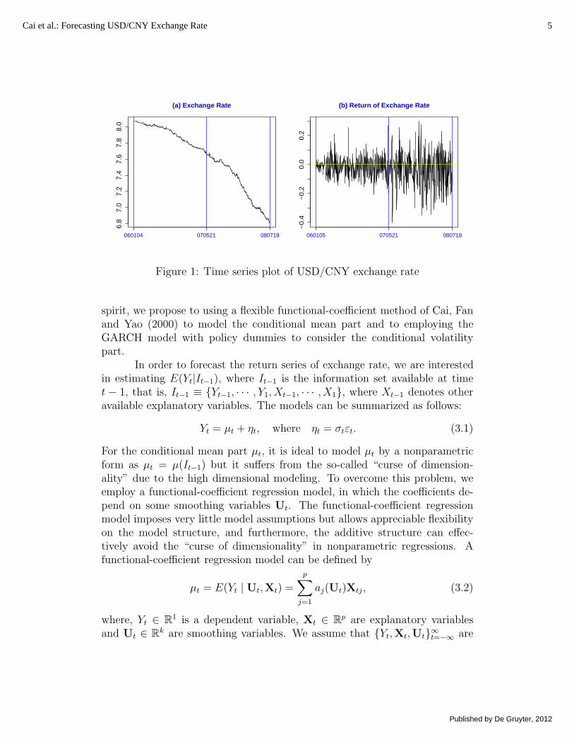
We concern the daily USD/CNY exchange rate series from January 4, 2006 toJuly 18, 2008, which forms a series of 619 observations. The data are avail-able from the website of Chinese State Administration of Foreign Exchange(http://www.safe.gov.cn/). Let Zt be the exchange rate on the tth day. Figure1(a) shows that the price series has an obvious decreasing time trend, whichreflects the fact of a gradual appreciation of RMB since 2006. Denote thereturn series by Yt = 100 log(Zt/Zt−1), the so-called scaled logarithmic differ-ence. Figure 1(b) presents the time series graph of the return of exchange rateand it clearly shows a structural change on May 21, 2007. On that day, theauthorities raised the float range of USD/CNY exchange rate from 0.3 percentto 0.5 percent.

3.2 The Model

Figure 1(b) shows that the return series is nonlinear but hard to be modeled byan existing parametric nonlinear model. However, any nonlinear model canbe approximated by a nonparametric time-varying parameter or functionalcoefficient linear model; see Granger (2008) and Cai (2010). Following this


6.8

7.0

7.2

7.4

7.6

7.8

8.0

060104 070521 080718

(a) Exchange Rate

−0.

4−

0.2

0.0

0.2

060105 070521 080718

(b) Return of Exchange Rate

Figure 1: Time series plot of USD/CNY exchange rate

spirit, we propose to using a flexible functional-coefficient method of Cai, Fanand Yao (2000) to model the conditional mean part and to employing theGARCH model with policy dummies to consider the conditional volatilitypart.

In order to forecast the return series of exchange rate, we are interestedin estimating E(Yt|It−1), where It−1 is the information set available at timet − 1, that is, It−1 ≡ {Yt−1, · · · , Y1, Xt−1, · · · , X1}, where Xt−1 denotes otheravailable explanatory variables. The models can be summarized as follows:

Yt = µt + ηt, where ηt = σtεt. (3.1)

For the conditional mean part µt, it is ideal to model µt by a nonparametricform as µt = µ(It−1) but it suffers from the so-called “curse of dimension-ality” due to the high dimensional modeling. To overcome this problem, weemploy a functional-coefficient regression model, in which the coefficients de-pend on some smoothing variables Ut. The functional-coefficient regressionmodel imposes very little model assumptions but allows appreciable flexibilityon the model structure, and furthermore, the additive structure can effec-tively avoid the “curse of dimensionality” in nonparametric regressions. Afunctional-coefficient regression model can be defined by

µt = E(Yt | Ut,Xt) =

p∑j=1

aj(Ut)Xtj, (3.2)

where, Yt ∈ R1 is a dependent variable, Xt ∈ Rp are explanatory variablesand Ut ∈ Rk are smoothing variables. We assume that {Yt,Xt,Ut}∞t=−∞ are



strictly stationary and {aj(·)pj=1} are measurable functions mapping from Rk

to R1; see Cai, Fan and Yao (2000) for details.For the conditional volatility part σt, a GARCH type model is used with

policy dummy variable. To address the structural change occurred on May 21,2007, a policy dummy variable Ct is considered, which takes a value of zerofor observations before that day and one for the remaining observations. Thatis,

Ct =

{0, when t < 20070521;1, when t ≥ 20070521.

We also add the same policy dummy variable in the conditional mean part.By combining (3.1) and (3.2), the forecasting model takes the following form:

Yt = aC(Ut)Ct +

p∑j=1

aj(Ut)Yt−j + ηt ≡p+1∑j=1

aj(Ut)Xtj + σtεt, (3.3)

σ2t = γ0 + γ1η

2t−1 + δ1σ

2t−1 + ασCt (3.4)

with γ0 > 0, γ1 ≥ 0, δ1 ≥ 0, and γ1+δ1 < 1, where Xtj = Yt−j, Xt,p+1 = Ct, Ut

is a univariate smoothing variable determined later and {aj(·)}, 1 ≤ j ≤ p+1,are continuous functions.

3.3 The Nonparametric Estimation

There are several nonparametric estimation techniques available for estimatingthe functional coefficient {aj(·)}. Here we employ the local linear regressionmethod due to its attractive properties such as the boundary correction andminimax efficiency; see Fan (1993) and Fan and Gijbels (1996). We assumethroughout that aj(·) has a continuous second derivative. Then, for any givengrid point u0 ∈ Rk, when Ut is in a neighborhood of u0, aj(Ut) is approximatedlocally at u0 by the Taylor expansion. That is, aj(Ut) ≈ aj(u0)+ aj(u0)

⊤(Ut−u0), where aj(u0) = ∂aj(u0)/∂u0. The local linear estimate is defined as

aj(u0) = aj, ˆaj(u0) = bj, where (aj, bj) minimizes the sum of locally weightedsquares:

n∑t=1

[Yt −

p+1∑j=1

(aj + b⊤j (Ut − u0)Xtj)

]2Kh(Ut − u0),

where Kh(·) = h−kK(·/h), K(·) is a kernel function on Rk, h > 0 is a band-width, and h → 0 as n → ∞. By moving u0 along the whole domain of Ut,the entire estimated surface of aj(u0) is obtained.


The data-driven fashion and optimal bandwidth is chosen by the nonpara-metric Akaike information criterion (AIC) developed by Hurvich, Simonoff andTsai (1998) and Cai and Tiwari (2000), which is specifically designed as anapproximately unbiased estimator of the expected Kullback-Leiber informa-tion criterion in nonparametric regression settings. Also, the nonparametricAIC can be used for choosing the “optimal” order p in model (3.3); see Caiand Tiwari (2000) for details.

Besides the above local linear estimation method, Huang and Shen (2004)proposed a global smoothing method based on a polynomial spline to estimatethe functional-coefficient model. One appealing feature of their method is thatthe functional coefficients can depend on different smoothing variables. How-ever, the local linear estimation has the advantage of utilizing local informationsufficiently and can obtain the minimax efficiency (Fan, 1993).

3.4 The Selection of Smoothing Variable

It is important to choose an appropriate smoothing variable Ut when applyingthe functional-coefficient regression model. Knowledge on physical backgroundof the data or economic theory and events may be very helpful. Some data-driven methods to choose the smoothing variables are also available, such asthe Akaike information criterion, cross-validation, and other criteria; see Cai,Fan and Yao (2000) and Fan, Yao and Cai (2003). We benefit from the factthat the value of RMB pegs to a basket of main currencies. The Governorof the People’s Bank of China, Mr. Xiaochuan Zhou, stated on August 9,2005 that the major currencies in the basket include US dollar (USD), Euro(EUR), Japanese Yen (JPY), and Korean Won (KRW). Therefore, we choosethe smoothing variable as a linear combination of the return series of threemajor exchange rates: EUR/USD, KRW/USD and JPY/USD as

Ut = βEUR · rEUR,t + βKRW · rKRW,t + βJPY · rJPY,t, (3.5)

where β = (βEUR, βKRW , βJPY ) are weights satisfying the identification condi-tion βEUR + βKRW + βJPY = 1, and rEUR,t, rKRW,t and rJPY,t are the returnseries of EUR/USD, KRW/USD and JPY/USD, respectively. The weights canbe automatically determined by the data because they are unknown. Noticethat model (3.3) becomes to the index functional coefficient model proposedin Fan, Yao and Cai (2003).

The weights β are estimated by a hybrid backfitting algorithm methodproposed by Fan, Yao and Cai (2003). Basically, the estimation method is analternating iteration between estimating the linear index through a one-step



scheme proposed by Bickel (1975) and estimating the functional coefficientsthrough an one-dimensional local linear smoothing method. To minimize theE(Y − Y )2, one should search for β to minimize

R(β) =1

n

n∑t=1

{Yt −

p+1∑j=1

aj(Ut)Xtj

}2

w(Ut),

where w(·) is a known weighting function. Suppose that β is the minimizerof the above equation, then R(β) = 0, where R(·) denotes the derivative ofR(·). For any β(0) close to β, we have the Taylor approximation 0 = R(β) ≈R(β(0))+R(β(0))(β−β(0)), where R(·) is the Hessian matrix of R(·). This leadsto the one-step iterative estimate similar to the Newton-Raphson procedure:

β(1) = β(0) − R(β(0))−1R(β(0)),

where β(0) is the initial value. At each iteration, we re-scale β(1) such that ithas unit sum. We refer the reader to the paper by Fan, Yao and Cai (2003)for details.

Alternatively, one might consider other smoothing variables used in theliterature, such as the moving average technique trading rule (MATTR)

Ut,MATTR =Yt−1∑L

j=1 Yt−j/L− 1

for certain L (say, L = 21), as in Brock, Lakonishock and Lebaron (1992) andHong and Lee (2003). Indeed, Ut,MATTR has a nice economic interpretation;see the aforementioned papers for details. Based on our empirical study, wefind that the linear combination of several main currencies versus US dollaroutperforms MATTR in terms of the nonparametric AIC criterion.

3.5 A Goodness-of-Fit Test

It is important to consider the goodness-of-fit of the nonparametric modelproposed above. For example, it is interesting to test whether the policydummy variable is significant.

Firstly, we test for the linear regression model against the nonparametricfunctional-coefficient regression model by employing the method proposed byCai, Fan and Yao (2000). The null hypothesis is defined as:

H0 : aj(Ut) = αj for 1 ≤ j ≤ p+ 1, (3.6)


so that model (3.3) becomes a pth order autoregressive model with an exoge-nous variable Ct, where {αj} are constant parameters in the AR(p). In otherwords, Ut does not have an impact on the USD/CNY exchange rate. In par-ticular, it is interesting to see if the policy dummy variable is significant. Thatis equivalent to testing the null hypothesis defined as

H0 : aC(Ut) = 0, (3.7)

which is to test a full nonparametric functional-coefficient regression modelagainst to a reduced nonparametric functional-coefficient regression model.To consider the test in (3.6) and (3.7), one can apply a generalized likelihoodratio (or generalized F-type) test proposed by Cai, Fan and Yao (2000) andstudied by Fan, Zhang and Zhang (2001), which can be constructed as

F =RSS0 −RSS1

RSS1

=RSS0

RSS1

− 1,

where RSS0 and RSS1 are the residual sum of squares under the null andalternative hypotheses respectively. The null hypothesis is rejected for largevalue of the test statistic. To calculate the p-value, a nonparametric wildbootstrap approach can be employed; see Cai, Fan and Yao (2000) for details.

3.6 Prediction Intervals

It is easy to see from (3.3) and (3.4) that the τth conditional quantile of Yt

given Ut and Xt is

qτ (Ut,Xt) =

p+1∑j=1

aj(Ut)Xtj + σt F−1ε (τ), (3.8)

where Fε(·) is the distribution of ε. Therefore, a naive (1−α)100% predictioninterval can be constructed as(

p+1∑j=1

aj(Ut)Xtj + σt F−1ε (α/2),

p+1∑j=1

aj(Ut)Xtj + σt F−1ε (1− α/2)

).

To make prediction interval in a nonparametric nature, the above quantileregression function in (3.8) is generalized to be more a general form as

qτ (Ut,Xt) = aC,τ (Ut)Ct +

p∑j=1

aj,τ (Ut)Xtj,



which was proposed by Cai and Xu (2008), where {aj,τ (·)} might depend on τ .To estimate {aj,τ (·)} nonparametrically, one can use a nonparametric quantileregression estimation procedure as in Cai and Xu (2008). Use the Taylorexpansion,

qτ (Ut,Xt) ≈ β⊤0,τXt + β⊤

1,τXt(Ut − u0),

and then find (β0,τ , β1,τ ) to minimize the following

Σnt=1ρτ

(Yt − β⊤

0,τXt − β⊤1,τXt(Ut − u0)

)Kh(Ut − u0),

where ρτ (z) = z(τ − I{z<0}) is the loss function and IA denotes the indicatorfunction of any set A. Then, the nonparametric estimation of aj,τ (u0) is the jth

element of β0,τ , so that the nonparametric estimation of qτ (u0,Xt) is β⊤0,τXt.

By changing the value of τ from 0 to 1, a set of quantile regressions areobtained. Particularly, when letting τ1 = 0.025 and τ2 = 0.975, then a 95%prediction interval is obtained and it is (qτ1(Ut,Xt), qτ2(Ut,Xt)).

4 Empirical Results

4.1 Policy Change and Structural Breaks

Although the functional coefficient model defined in (3.2) is sufficiently tomodel continuously time varying features of the exchange rate by assumingthat the time varying coefficients depend on a smooth function of other ran-dom variables, it would be still helpful to include policy changes or discretestructural breaks into the functional coefficient regressions. We notice thatthere exists an important policy change during the sample period. On May21, 2007, the float range of RMB exchange rate against the US dollar wasraised from 0.3 percent to 0.5 percent. Figure 1(b) demonstrates that largerdaily volatility of returns of exchange rate can be observed after that datethan that before May 21, 2007. We include a policy dummy Ct, which takes avalue of zero before that date and one on or after that date, into the functionalcoefficient regression.

The sup Wald test (Andrews, 1993) detects a break at the date of October16, 2007, which is about 5 months later than the policy change date. A breakdummy is also defined by taking a value of zero before October 16, 2007 andone on or after that date. Now we consider two competing models: one isthe model in (3.3) with a policy dummy and the other is the model includingboth policy dummy and break dummy. The encompassing (ENC-NEW) test(Clark and McCracken, 2001) is employed to test whether the model including


the break dummy can improve the post sample forecast accuracy. The nullhypothesis is that the nested model is better than the model in the alternativewhich includes both dummies. The p-value of the test is about 0.86 then wecan not reject the null. We also compute the mean square forecasting errors(MSFEs) and mean average forecasting errors (MAFEs) for four alternativemodels: (1) a functional coefficient model with a policy dummy; (2) a func-tional coefficient model without dummies; (3) a functional coefficient modelwith a break dummy; and (4) a functional coefficient model with both dum-mies. The results conclude that the functional coefficient model with a policydummy dominates all others in terms of post sample forecasting errors.1

4.2 Estimation Results

For the conditional mean part, we use an index functional-coefficient regressionmodel with the coefficients depending on the smoothing variable Ut given in(3.5). By using the nonparametric AIC method and the hybrid backfittingalgorithm, the selected optimal bandwidth is h = 1.2, the selected optimal lagterm is p = 2 and the selected optimal weights are β = (0.2967, 0.3843, 0.3190).The smoothing variable is constructed by a linear combination of the returnseries of EUR/USD, KRW/USD and JPY/USD with the estimated weightsβ and its time series plot is presented in Figure 2. The estimated functionalcoefficient curves are displayed in Figure 3. Finally, both goodness-of-fit

0 100 200 300 400 500 600

−2

−1

01

2

Smoothing Variable

Figure 2: Time series plot of smoothing variable series.

1The MSFEs for all models are 0.0141, 0.0150, 0.0148 and 0.0151, respectively. TheMAFEs are 0.1016, 0.1023, 0.1046 and 0.1055, respectively.



−1 0 1 2

−0.

6−

0.4

−0.

20.

0USD/CNY: 1st order Lag term

−1 0 1 2

−0.

20.

00.

20.

40.

6

USD/CNY: 2nd order Lag term

−1 0 1 2

−2.

0−

1.5

−1.

0−

0.5

0.0

CONTROL BNAD

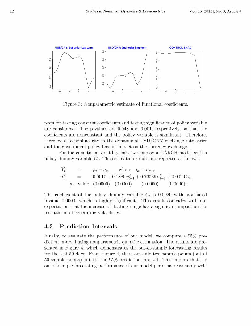
Figure 3: Nonparametric estimate of functional coefficients.

tests for testing constant coefficients and testing significance of policy variableare considered. The p-values are 0.048 and 0.001, respectively, so that thecoefficients are nonconstant and the policy variable is significant. Therefore,there exists a nonlinearity in the dynamic of USD/CNY exchange rate seriesand the government policy has an impact on the currency exchange.

For the conditional volatility part, we employ a GARCH model with apolicy dummy variable Ct. The estimation results are reported as follows:

Yt = µt + ηt, where ηt = σtεt,

σ2t = 0.0010 + 0.1880 η2t−1 + 0.73589σ2

t−1 + 0.0020Ct

p− value (0.0000) (0.0000) (0.0000) (0.0000).

The coefficient of the policy dummy variable Ct is 0.0020 with associatedp-value 0.0000, which is highly significant. This result coincides with ourexpectation that the increase of floating range has a significant impact on themechanism of generating volatilities.

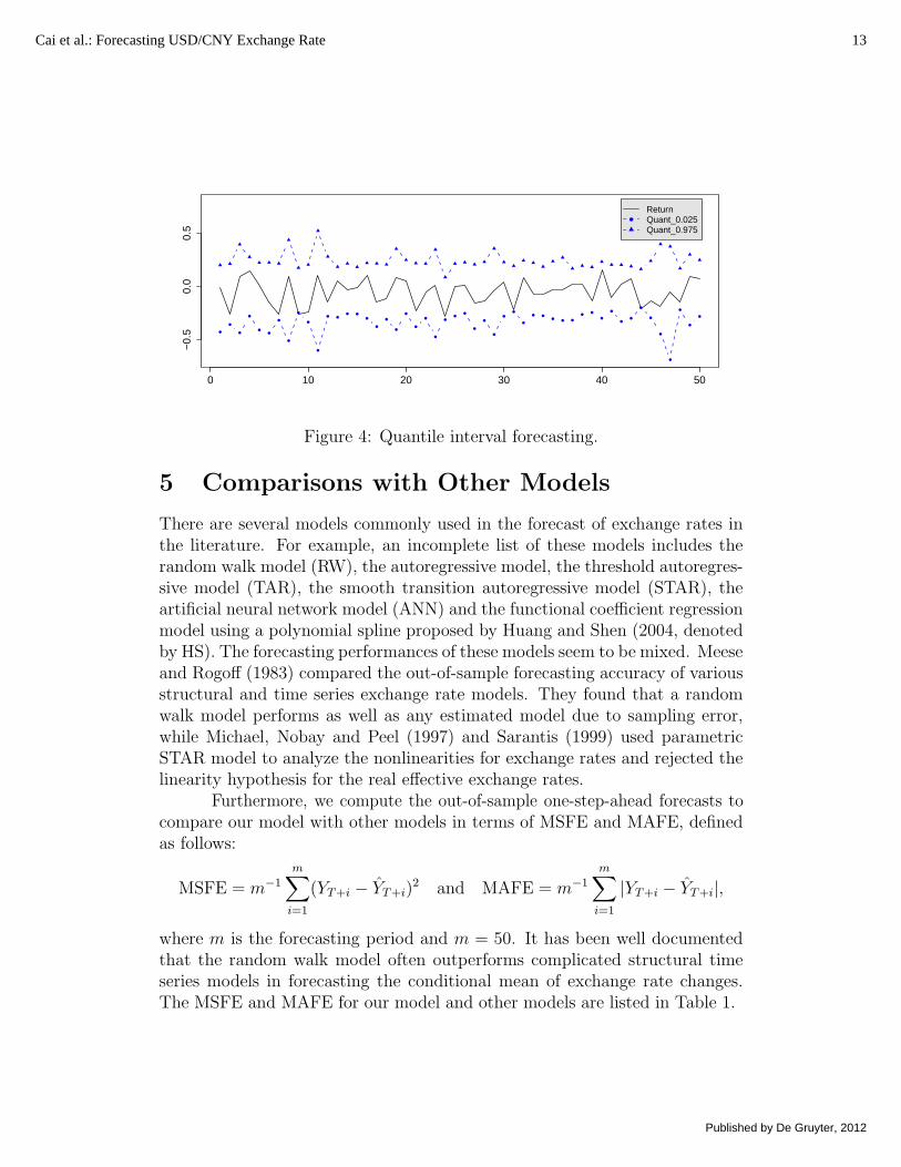
4.3 Prediction Intervals

Finally, to evaluate the performance of our model, we compute a 95% pre-diction interval using nonparametric quantile estimation. The results are pre-sented in Figure 4, which demonstrates the out-of-sample forecasting resultsfor the last 50 days. From Figure 4, there are only two sample points (out of50 sample points) outside the 95% prediction interval. This implies that theout-of-sample forecasting performance of our model performs reasonably well.


0 10 20 30 40 50

−0.

50.

00.

5

ReturnQuant_0.025Quant_0.975

Figure 4: Quantile interval forecasting.

5 Comparisons with Other Models

There are several models commonly used in the forecast of exchange rates inthe literature. For example, an incomplete list of these models includes therandom walk model (RW), the autoregressive model, the threshold autoregres-sive model (TAR), the smooth transition autoregressive model (STAR), theartificial neural network model (ANN) and the functional coefficient regressionmodel using a polynomial spline proposed by Huang and Shen (2004, denotedby HS). The forecasting performances of these models seem to be mixed. Meeseand Rogoff (1983) compared the out-of-sample forecasting accuracy of variousstructural and time series exchange rate models. They found that a randomwalk model performs as well as any estimated model due to sampling error,while Michael, Nobay and Peel (1997) and Sarantis (1999) used parametricSTAR model to analyze the nonlinearities for exchange rates and rejected thelinearity hypothesis for the real effective exchange rates.

Furthermore, we compute the out-of-sample one-step-ahead forecasts tocompare our model with other models in terms of MSFE and MAFE, definedas follows:

MSFE = m−1

m∑i=1

(YT+i − YT+i)2 and MAFE = m−1

m∑i=1

|YT+i − YT+i|,

where m is the forecasting period and m = 50. It has been well documentedthat the random walk model often outperforms complicated structural timeseries models in forecasting the conditional mean of exchange rate changes.The MSFE and MAFE for our model and other models are listed in Table 1.



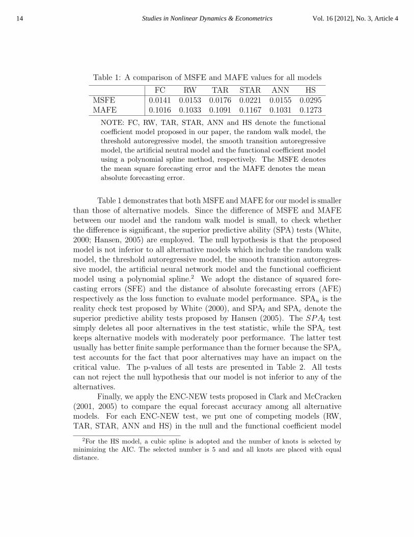
Table 1: A comparison of MSFE and MAFE values for all models

FC RW TAR STAR ANN HSMSFE 0.0141 0.0153 0.0176 0.0221 0.0155 0.0295MAFE 0.1016 0.1033 0.1091 0.1167 0.1031 0.1273

NOTE: FC, RW, TAR, STAR, ANN and HS denote the functionalcoefficient model proposed in our paper, the random walk model, thethreshold autoregressive model, the smooth transition autoregressivemodel, the artificial neutral model and the functional coefficient modelusing a polynomial spline method, respectively. The MSFE denotesthe mean square forecasting error and the MAFE denotes the meanabsolute forecasting error.

Table 1 demonstrates that both MSFE and MAFE for our model is smallerthan those of alternative models. Since the difference of MSFE and MAFEbetween our model and the random walk model is small, to check whetherthe difference is significant, the superior predictive ability (SPA) tests (White,2000; Hansen, 2005) are employed. The null hypothesis is that the proposedmodel is not inferior to all alternative models which include the random walkmodel, the threshold autoregressive model, the smooth transition autoregres-sive model, the artificial neural network model and the functional coefficientmodel using a polynomial spline.2 We adopt the distance of squared fore-casting errors (SFE) and the distance of absolute forecasting errors (AFE)respectively as the loss function to evaluate model performance. SPAu is thereality check test proposed by White (2000), and SPAl and SPAc denote thesuperior predictive ability tests proposed by Hansen (2005). The SPAl testsimply deletes all poor alternatives in the test statistic, while the SPAc testkeeps alternative models with moderately poor performance. The latter testusually has better finite sample performance than the former because the SPAc

test accounts for the fact that poor alternatives may have an impact on thecritical value. The p-values of all tests are presented in Table 2. All testscan not reject the null hypothesis that our model is not inferior to any of thealternatives.

Finally, we apply the ENC-NEW tests proposed in Clark and McCracken(2001, 2005) to compare the equal forecast accuracy among all alternativemodels. For each ENC-NEW test, we put one of competing models (RW,TAR, STAR, ANN and HS) in the null and the functional coefficient model

2For the HS model, a cubic spline is adopted and the number of knots is selected byminimizing the AIC. The selected number is 5 and and all knots are placed with equaldistance.


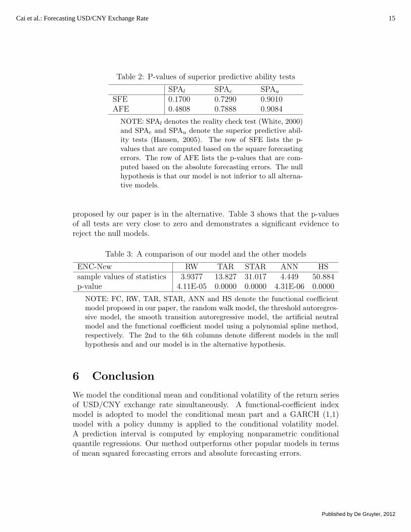
Table 2: P-values of superior predictive ability tests

SPAl SPAc SPAu

SFE 0.1700 0.7290 0.9010AFE 0.4808 0.7888 0.9084

NOTE: SPAl denotes the reality check test (White, 2000)and SPAc and SPAu denote the superior predictive abil-ity tests (Hansen, 2005). The row of SFE lists the p-values that are computed based on the square forecastingerrors. The row of AFE lists the p-values that are com-puted based on the absolute forecasting errors. The nullhypothesis is that our model is not inferior to all alterna-tive models.

proposed by our paper is in the alternative. Table 3 shows that the p-valuesof all tests are very close to zero and demonstrates a significant evidence toreject the null models.

Table 3: A comparison of our model and the other models

ENC-New RW TAR STAR ANN HSsample values of statistics 3.9377 13.827 31.017 4.449 50.884p-value 4.11E-05 0.0000 0.0000 4.31E-06 0.0000

NOTE: FC, RW, TAR, STAR, ANN and HS denote the functional coefficientmodel proposed in our paper, the random walk model, the threshold autoregres-sive model, the smooth transition autoregressive model, the artificial neutralmodel and the functional coefficient model using a polynomial spline method,respectively. The 2nd to the 6th columns denote different models in the nullhypothesis and and our model is in the alternative hypothesis.

6 Conclusion

We model the conditional mean and conditional volatility of the return seriesof USD/CNY exchange rate simultaneously. A functional-coefficient indexmodel is adopted to model the conditional mean part and a GARCH (1,1)model with a policy dummy is applied to the conditional volatility model.A prediction interval is computed by employing nonparametric conditionalquantile regressions. Our method outperforms other popular models in termsof mean squared forecasting errors and absolute forecasting errors.



Since the Chinese government made several reforms on the daily USD/CNYexchange rate, so that the policy changes should have an impact on the dy-namic of the exchange rate. We include policy dummy variables into theconditional mean model and the conditional volatility as well. The daily floatlimit of RMB exchange against USD was relaxed from 0.3 percent to 0.5 per-cent on May 21, 2007. A dummy corresponding to the policy change wasincluded and the tests show that the dummy is highly significantly both in theconditional mean and the conditional volatility models, which provides evi-dence that gradual liberalization can improve the flexibility of Chinese foreignexchange rate.

Moreover, the goodness-of-fit test demonstrates that the functional coeffi-cients is significantly nonconstant, varying with a linear combination of othercurrencies which includes the Euro, Japanese yen and Korean won. Using thechanges of the values of other currencies is helpful to predict the dynamicsof the USD/CNY exchange rate. Our empirical results partially support therecent findings of Frankel and Wei (2007). They found a modest but stead in-crease in weights of non-dollar currencies in the basket to determine the valueof RMB, which would increase the flexibility of China’s exchange rate.

References

Andrews, D.W. (1993): “Tests for Parameter instability and structural changewith unknown change point,” Econometrica 61, 821-856.

Bickel, P. (1975): “One-step Huber estimates in the linear model,” Journalof the American Statistical Association, 70, 428-434.

Bollerslev, T. (1986): “Generalized autoregressive conditional heteroscedas-ticity,” Journal of Econometrics, 31, 307-327.

Bollerslev, T. (1987): “A conditionally heteroscedastic time series model forspeculative prices and rates of return,” Review of Economics and Statis-tics, 69, 542-547.

Bollerslev, T. (1990): “Modelling the coherence in short-run nominal ex-change rates: multivariate generalized ARCH approach,” Review of Eco-nomics and Statistics, 72, 498-505.

Branstetter, L. and N. Lardy (2008): “China’s embrace of globalization,”in Loren Brandt and Thomas G. Rawski, ed., China’s Great EconomicTransformation, Cambridge: Cambridge University Press, 633-682.

Brock, W., D. Hsieh and B. Lebaron (1991): Nonlinear Dynamics, Chaos,and Instability: Statistical Theory and Economic Inference, Cambridge:MIT Press.


Brock, W., J. Lakonishock, and B. Lebaron (1992): “Simple technical tradingrules and the stochastic properties of stock returns,” Journal of Finance,47, 1731-1764.

Cai, Z. (2010): “Functional coefficient models for economic and financialdata,” in Frederic Ferraty and Yves Romain, ed., Oxford Handbook ofFunctional Data Analysis, Oxford: Oxford University Press, 166-186.

Cai, Z., J. Fan and Q. Yao (2000): “Functional-coefficient regression modelsfor nonlinear time series,” Journal of the American Statistical Associa-tion, 95, 941-956.

Cai, Z. and R. Tiwari (2000): “Application of a local linear autoregressivemodel to BOD time series,” Environmetrics, 11, 341-350.

Cai, Z. and Q. Xu (2008): “Nonparametric quantile estimations for dynamicsmooth coefficient models,” Journal of the American Statistical Associ-ation, 103, 1595-1608.

Clark, T.E. and M.W. McCracken (2001): “Tests of equal forecast accuracyand encompassing for nested models,” Journal of Econometrics, 105,85-110.

Clark, T.E. and M.W. McCracken (2005): “The power of tests of predictiveability in the presence of structural breaks,” Journal of Econometrics,124, 1-31.

Dielbond, F.X. and J.A. Nason (1990): “Nonparametric exchange rate pre-diction?,” Journal of International Economics, 28, 315-332.

Engle, R., T. Ito and W. Lin (1990): “Meteor showers or heat waves?Heteroskedastic intra-daily volatility in the foreign exchange market,”Econometrica 58, 525-542.

Fan, J. (1993): “Local linear regression smoothers and their minimax,” TheAnnals of Statistics, 21, 196-216.

Fan, J. and I. Gijbels (1996): Local Polynomial Modelling and Its Applica-tions, London: Chapman and Hall.

Fan, J., Q. Yao and Z. Cai (2003): “Adaptive varying-coefficient linear mod-els,” Journal of the Royal Statistical Society, Series B, 65, 57-80.

Fan, J., C. Zhang and J. Zhang (2001): “Generalized likelihood ratio statisticsand Wilks phenomenon,” The Annals of Statistics, 29, 153-193.

Frankel, J. and S. Wei (2007): “Assessing China’s exchange rate regime,”Economic Policy, 22, 575-627.

Gencay, R. (1999): “Linear, non-linear and essential foreign exchange rateprediction with simple technical trading rules,” Journal of InternationalEconomics, 47, 91-107.



Granger, C. (2008): “Non-linear models: Where do we go next time varyingparameter models?,” Studies in Nonlinear Dynamics & Econometrics,12(3), 1-9.

Hansen, P. R. (2005): “A test for superior predictive ability,” Journal ofBusiness & Statistics, 23, 365-380.

Hong, Y. and T. Lee (2003): “Inference on via generalized spectrum andnonlinear time series models,” The Review of Economics and Statistics,85, 1048-1062.

Huang, J.Z. and H. Shen (2004): “Functional coefficient regression modelsfor non-linear time series: a polynomial spline approach ,” ScandinavianJournal of Statistics, 31, 515-534.

Hurvich, C., J. Simonoff and C. Tsai (1998): “Smoothing parameter selec-tion in nonparametric regression using an improved Akaike informationcriterion,” Journal of the Royal Statistical Society, Series B, 60, 271-293.

Kuan, C. and T. Liu (1995): “Forecasting exchange rates using feedforwardand recurrent neural networks,” Journal of Applied Econometrics, 10,347-364.

Meese, R. and K. Rogoff (1983): “Empirical exchange rate models of the sev-enties: Do they fit out of sample?,” Journal of International Economics,14, 3-24.

Meese, R. and A. Rose (1991): “An empirical assessment of non-linearitiesin models of exchange rate determination,” Review of Economic Studies,58, 603-619.

Michael, P., A. Nobay and D. Peel (1997): “Transactions costs and nonlin-ear adjustment in real exchange rates: An empirical investigation,” TheJournal of Political Economy, 105, 862-879.

Mizrach, B. (1992): “Multivariate nearest-neighbor forecasts of EMS ex-change rates,” Journal of Applied Econometrics, 7, 151-163.

Sarantis, N. (1999): “Modeling non-linearities in real effective exchange rates,”Journal of International Money and Finance, 18, 27-45.

West, K. and D. Cho (1995): “The predictive ability of several models ofexchange rate volatility,” Journal of Econometrics, 69, 367-391.

White, H. (2000): “A reality check for data snooping,” Econometrica, 68,1097-1126.


Copyright of Studies in Nonlinear Dynamics & Econometrics is the property of De Gruyterand its content may not be copied or emailed to multiple sites or posted to a listserv withoutthe copyright holder's express written permission. However, users may print, download, oremail articles for individual use.

a new forecasting model for usd/cny exchange rate

Documents