A New Approach for Constructing Home Price Indices:

The Pseudo Repeat Sales Model and Its Application in China

Xiaoyang GUO1,2, Siqi ZHENG1,*, David GELTNER2 and Hongyu LIU1 (1: Department of Construction Management and Hang Lung Center for Real Estate, Tsinghua

University; 2: Center for Real Estate, Massachusetts Institute of Technology;

* Contact author, zhengsiqi@tsinghua.edu.cn) This version: December 25, 2013 Abstract: This paper develops a “pseudo repeat sale” estimation sample construction procedure (ps-RS) to construct more reliable and less biased quality-controlled price indices for newly-constructed homes. The method may be useful wherever new housing development is of sufficiently large scale and homogeneous. Such circumstances characterize many emerging market countries, and here we apply the technique in China. We match two very similar new sales within a defined matching space. Here we test three versions of matching spaces – complex, phase, and building. We then regress the within-pair price differentials onto time dummies and the differentials in unit-specific physical attributes. Locational and community variations, as well as many unobservable or difficult to measure physical attribute variations, are cancelled out in the model, and thereby controlled for. The building-version ps-RS index does the best job in this regard because its within-pair differential is the smallest. We further introduce a “hedonic value” distance metric criterion so that one can deal flexibly with the trade-off between the within-pair “similarity” and the sample size. We explicate and demonstrate formal signal-to-noise oriented metrics of index quality, which can be superior to traditional standard errors based metrics, and we use the new metrics to compare index construction methodologies. The ps-RS approach addresses the problem of lack of repeat-sales data in emerging markets and newly constructed properties and the omitted variables problem in the hedonic method. It also addresses the traditional problems with the classical same-property repeat-sales model in terms of small sample sizes and sample selection bias. The present paper tests the ps-RS method using a large-scale micro transaction data set of new home sales from January 2006 to June 2011 (444,596 observations) in Chengdu, Sichuan Province, China. The resulting complex-based ps-RS index essentially parallels the hedonic index, suggesting that the hedonic index is not superior to that version of the ps-RS index in terms of systematic results. The phase-based ps-RS index has a lower growth trend and the building-based version lower still, indicating omitted variables relating to the physical quality of the units are

1

not well controlled for in the hedonic, and suggesting that the building-based version of the ps-RS index provides the greatest control for such quality differences. Building-based ps-RS indices with different distance metric thresholds are almost the same. Compared to the hedonic, the ps-RS provides a smoother index indicating less random estimation error (or “noise”). Keywords: Residential Price index; repeat sale; hedonic; pseudo repeat sale index, matched-sample estimation, rapid urbanization

2

1. Introduction

In the world of transaction price indices used to track the dynamics in housing

markets, the problem of controlling for heterogeneity in the homes transacting in

different periods of time is perhaps the most crucial challenge. The simple mean or

median values of all the sale prices per square meter each period will not produce

good price indices because the location, size, quality, and components of the homes

being sold keep changing over time. The two major methods in the academic

literature for addressing this challenge are the hedonic and repeat sales regressions. Of

these two, in the U.S., only the repeat-sales approach has seen widespread regular

production and publication in official or industry statistics (for example, the FHFA

and S&P/Case-Shiller home price indices).

In Chinese cities, as a representative case in this paper, we face two unique features in

that country’s urban residential market, features which also characterize development

in many emerging market countries. First, new home sales account for an

exceptionally large share of total sales in China (87% in 2010) due to a growth rate in

the economy and urbanization that in the case of China has been truly unprecedented

in world history. Thus, the classical repeat sales (RS) approach is of very limited

usefulness because the typical housing unit in China has only appeared once on the

market. Yet the hedonic method may face more than its usual challenges because the

omitted variables problem may be more severe in Chinese cities due to very rapid

evolution of urban spatial structure, infrastructure construction, and (most difficult to

observe) the quality and features and amenities within the housing units themselves

(such as apartment design, appliances, finishes, and HVAC) as household income

rises at an extremely rapid rate. Secondly, housing development in many high-density

cities, such as those in Mainland China, Taiwan, Singapore and many other Asian

cities, occurs at a uniquely large scale and with a high degree of homogeneity in the

units built within the typical residential “complex”. In each complex, a number of

buildings are constructed containing altogether hundreds or even thousands of units

3

all having essentially the same location, architecture design, structure, appliances and

finishes.

The proposal in this paper is to develop a new type of “repeat sales” model, which we

dub “pseudo repeat sales” (ps-RS). Fundamentally similar to the matched-sample

procedure recently proposed by McMillen (2012) in that the price observation pairs

used in the regression are not actually repeat-sales of the same property, our proposal

is a new matching criterion that we think is particularly appropriate for Chinese cities

and other high-density cities where large-scale residential complexes dominate the

urban housing development. We deal with the omitted variables issue by employing a

within-building matching criterion instead of the more stringent, same-unit criterion

of the classical RS approach1. This approach not only addresses the problem of lack

of repeat-sales data and problematical hedonic variables observation, but also

addresses the traditional problems with the classical repeat-sales model of small

sample sizes and sample selection bias in properties with repeated sales, as the ps-RS

procedure, like a hedonic price index, uses all of the transactions data. More

specifically, the proposed model is (in fact must be) a hybrid repeat sales/hedonic

model of the type that has been demonstrated to have desirable features in the

econometric literature, because the paired units in the ps-RS are not identical. The

hybrid (hedonic) component of our model is small and relies only on variables for

which good data can be easily obtained, because it only has to control for differences

between units within the same building. We believe the ps-RS still retains essentially

the characteristics of a “repeat sales” model. In this paper we present an argument and

evidence that the ps-RS can produce a more reliable and accurate picture of home

price appreciation in these very important markets.

1 The matching criterion can also be applied to sales across different buildings but within the same phase (several buildings constructed at the same time), or within the same complex. However, as we will discuss below, larger matching spaces (across buildings) appear to be less effective in mitigating the problem of omitted variables and controlling for quality differences. Our empirical results indicate that the within-building criterion is the best choice in our study market, the metropolitan area of Chengdu, Sichuan.

4

The rest of this paper is organized as follows: Section Two will present some relevant

background and literature review. Section three describes the features of the

new-home market in Chinese cities and how those features affect the choice of

housing price index construction methodology. We describe in detail our approach for

developing the ps-RS index in Section Four. After data description in Section Five,

the index calculation results for our demonstration city of Chengdu are presented in

Section Six, including a quantitative comparison of the ps-RS with the standard

hedonic method (which is the only realistic alternative since classical same-property

repeat sales is not possible for new housing). Section Seven concludes.

2. Background & Literature Review

The hedonic approach goes back to Kain and Quigley (1970), who decomposed the

components of housing price dynamics using the hedonic model, from which a

quality-controlled housing price index is generated by controlling for home

transactions’ physical and location attributes. Other pioneers of hedonic price

modeling were Court (1939), Griliches (1961), and Rosen (1974). Two alternative

methods have been proposed to construct a hedonic housing price index. The first

method assumes constant relative preferences for housing attributes over time, and

estimates a single hedonic regression for the whole historical sample (pooled

database), using time-dummies to capture the price evolution over time, and

constructing the price index from the coefficients of those time dummies. The second

method (referred to as “chained hedonic”) is to run separate cross-sectional hedonic

regressions for each period, and construct the price index as the predicted value from

each period’s regression model of a standard (or “representative”) housing unit that is

held constant across time.

The repeat sales model was introduced first by Bailey et al (1963) to calculate a

housing price change indicator using only properties that sold twice or more in the

historical sample. The basic idea is to regress the percentage price changes (or log

5

differences) between consecutive sales of the same properties onto a right-hand-side

data matrix that consists purely of time-dummy variables corresponding to the

historical periods in the price index. The time-dummies assume a value of zero before

the first sale and after the second sale.2 The RS model was largely ignored for two

decades before being independently rediscovered (and enhanced) by Case and Shiller

(1987, 1989).

The repeat sales model has some advantages and disadvantages from an econometric

perspective. It has less ability than the hedonic to elucidate the causes of the price

change dynamics. Especially in the case of the chained separate-regressions procedure,

hedonic indexes allow an analysis of the detailed causal factors or correlates (e.g.,

whether price growth is due to the opening of a new subway station or a new school).

But whatever the cause of price changes, the result is the same in terms of asset price

and value impact for the property investor/owner. The repeat sales model trades off an

ability to more deeply analyze the causal structure or correlates of price changes from

an urban economics or national income and product accounting perspective, for a

more parsimonious specification that has less challenging data requirements, and

leaves less room for debate about exactly what is the “correct” or “best” model

specification, and which may be more directly relevant to home-owner or investor

experiences. These features can give the RS a practical advantage for the purpose of

constructing an official or commercially produced index that must be updated and

published regularly primarily simply to track price change over time.

From an econometric perspective, the repeat sales model is theoretically equivalent to

the pooled-database hedonic model, as it is the differential transformation of that

hedonic model, assuming that the coefficients of the housing attributes are constant,

as demonstrated by Clapp and Giacotto (1992). Potentially different results from the

2 There are two equivalent specifications. Estimating the periodic changes (returns) directly, the periods between the first and second sale have dummy variable values of one, zero otherwise. Estimating the cumulative price levels directly (relative to the base period) the time dummies are all zero except negative one for the time of the first sale and positive one for the time period of the second sale within each same-property consecutive sale transactions.

6

two procedures then come only from the difference in the sample selection of the

estimation database, with only properties having sold more than once able to be

included in the repeat-sales model’s sample. Therefore, the repeat sales model can be

treated as a special estimation sample case of the pooled-database hedonic.3

In spite of the popularity of both approaches, the discussion about their shortcomings

has never stopped in the urban economics and econometrics literature. The hedonic

model is perhaps superior in theory (especially the chained hedonic). But hedonic

models suffer from data and specification challenges. The chained separate-regression

procedure requires very large datasets. Both hedonic procedures require lots of good

hedonic data, and are vulnerable to specification problems, most notably omitted

variables. This can make hedonic models weaker in practice, especially for practical

purposes of producing an official, frequently updated and regularly published index

covering all the major markets in a large country, such as an agency like the China

National Bureau of Statistics might contemplate. Indeed, as a result of data problems

and omitted variables, it has been claimed that all hedonic based housing price indices

are more or less biased (Quigley, 1995). The parsimony of the repeat sales model, on

the other hand, tends to make it more robust to omitted variables. However, the

weakness of the classical same-property RS procedure is the limited sample size and

sample selection bias caused by the model’s need for repeat-sales of same properties.

Sample selection bias or small sample sizes can be addressed in various ways, but

3 It should be noted that while the RS model can be derived as the differential of the pooled-database hedonic model, it need not be so derived. The RS model can stand on its own as a primal specification. As such, the only assumption is that the time-dummy coefficients represent all of the longitudinal change in pricing, from whatever source or cause, between the first and second sales of the same properties. Viewed from this perspective, the same-property RS model directly measures the round-trip price-change experiences of home-owners or investors in the property market, a subject that is subtly distinct from average property price change but that is of interest and importance in its own right. Viewed from the hedonic perspective, such price changes may reflect any combination of three sources: (i) changes in the values of the hedonic attributes of the property (such as, size, age, number of bedrooms, bathrooms, etc.); (ii) changes in the hedonic coefficients (changes in the implicit prices of the hedonic attributes); or (iii) movement in an “intercept” in the cross-sectional hedonic specification (which would presumably largely reflect changes in location value and general market conditions, the relative balance between supply and demand). The pooled-database hedonic approach attempts to control for (i) by specifying and estimating all of the hedonic attributes. The classical same-property RS model controls for (i) by presuming that changes in the values of the hedonic attributes are minimal within the same unit over time. Only the chained separate-regressions hedonic procedure can control for both (i) and (ii), thereby allowing full causal analysis of the price changes and limiting the index price movement to purely reflect source (iii), changes in location value and the housing market supply/demand balance (by constructing an index based purely on changes in the intercepts).

7

these remain concerns in the classical RS index (Meese and Wallace, 1997; Gatzlaff

and Haurin, 1998).4

A number of methods have been proposed to address the problems in both the hedonic

and repeat-sales approaches. Case and Quigley (1991) developed a hybrid model to

combine the advantages, and avoid the weaknesses, of the hedonic and repeat sales

models. Case, Pollakowski and Wachter (1991) empirically tested and compared three

groups of housing price indices models, finding that the hybrid model appeared to be

empirically more efficient than either the hedonic or repeat sales model, and that the

difference between the results of the hedonic and hybrid comes from the systematic

differences between single transactions and repeat transactions. Similar results have

been verified by a large literature (Englund, Quigley and Redfearn, 1999; Hansen,

2009; among others).

An interesting perspective to take on the repeat sales model, which is relevant to the

current paper, is to view the repeat sales specification as one (extreme) solution to a

matching problem. The objective is to match, or pair together, individual property sale

observations across time, according to some criterion so as to cancel out as much as

possible the unobservable attributes, making the model more parsimonious and robust

so that it does not need as much good hedonic data. As has been pointed out by

McMillen (2012), in the extreme, if the matching criterion picks pairs of properties

that have no difference in any of the hedonic attributes that matter in price change

dynamics, then a matched-sample index will be just as good as an ideal same-property

repeat-sales index.5 In the classical repeat sales model, the matching criterion is

4 It should also be noted that in practice, repeat-sales estimation sample sizes may not necessarily be much if any smaller than hedonic estimation sample sizes once one considers the need for all of the transaction observations to include good values for a range of hedonic variables for the hedonic model, whereas the repeat-sales model needs only the sale price and date. 5 Indeed, McMillen points out that in some respects a matched-sample index can be superior to a traditional same-property repeat-sales index. For example, it may allow more transaction observation pairs, a larger sample size, as it is not limited to properties that have actually transacted twice. Furthermore, McMillen proposes a sample construction procedure which anchors each matched pair onto the index historical base period for its first sale. This allows a more equal weighting of property attributes across history (effectively a Laspeyres price index), and reduces the infamous “backward adjustments” (historical revisions) problem in classical same-property repeat-sales indices, which can cause practical problems for some index uses. These problems can in principle also

8

extreme in that a sale is matched only to its previous or subsequent sale of the exact

same property, so that as much as possible of the variation in location and physical

attributes are cancelled out (except for property age and possibly some renovations in

the neighborhood or improvements in the house).

McMillen’s matching criterion is based on each sold property’s sale propensity score

in a logit sales probability model of all the properties sold in the base period and all

the properties sold in subsequent period “t” (separate logit models for each period “t”

in the price index). Each property sold in the base period is matched with one property

sold in each subsequent period in the index, thus creating n0T matched pairs in the

index estimation sample, where n0 is the number of sales in the base period and T is

the number of historical periods in the index. The McMillen procedure is essentially a

data preprocessing procedure for building an estimation sample for the price change

regression model to use, and it can create a larger estimation sample than the number

of actual empirical same-property sales pairs.6 But mainland Chinese cities typically

do not have the problem of small transaction sample sizes for housing price data, as

the housing markets are huge and rapidly growing. And the McMillen matching

procedure does require good hedonic data, which we have noted is a problem in

Chinese data. Deng, McMillen and Sing (2011) have applied the McMillen method to

Singapore’s residential market with some success. But the Singapore market has much

better hedonic data than mainland China and lacks some of the hedonic modeling

challenges found in Chinese cities due to the extremely rapid urbanization and income

growth in China. In fact, in Shiller’s book (2003) and his seminal papers (Case and

Shiller, 1987, 1989), he talks about generalizing their repeat-sale method to a “class or

kind of subjects”, and mentions condominiums as being particularly relevant.

be mitigated by our pseudo-RS matching procedure. 6 As such, it provides a potential complement to other procedures proposed in the literature to be applied to other stages of the index production process to address the widespread problem of small transaction sample sizes. For example, Goetzmann (1992), McMillen (2001), and Francke (2010), have proposed estimation methods or specifications for the regression model itself. And Bokhari and Geltner (2012) have proposed a frequency conversion method in the production of the final index from the price change regression results. Procedures applied to the three sequential stages of the index production process (estimation sample preparation, regression model estimation, and index production from the regression results) can in principle be applied together, to magnify their effectiveness.

9

Therefore, both McMillen’s matching model and our ps-RS matching model can be

essentially regarded as applications of Shiller’s proposal.

3. Features in China’s Urban Housing Market and Their Implications for Price Index Construction

Before the 1980s, urban housing in China was allocated to urban residents as a

welfare good by their employer (the work unit) through the central planning system.

Workers enjoyed different levels of housing welfare according to their office ranking,

occupational status, working experience and other merits. Governments and work

units were responsible for housing construction and residential land was allocated

through central planning (Zheng et. al., 2006). Since the 1980s, most of the work-unit

housing units have been privatized. By the end of the 1990s, housing procurement by

work units for their employees had officially ended and new homes would be built

and sold in the market (Fu et al, 2000). Developable land was supplied and regulated

by the government through long-term leases. The real estate market took off, and

massive land development took place in many Chinese cities. Sales of newly built

residential properties reached 933 million square meters in 2010, with an average

annual growth rate of about 20% in the last 10 years.7

With the fastest urbanization in world history (almost 500 million people urbanized

from 1980 to 2010), massive investment in urban transport infrastructure, and the

rapid growth of the service sector in Chinese cities since the beginning of the 1990s, a

more specialized land-use pattern has emerged. We see that the central business

district (CBD) has greatly expanded while residential land use has extended into

7 To put this in some perspective, in the U.S., with one-fourth the population of China, the peak year of housing construction, 2005, saw less than 300 million square meters built (in houses that were on average more than twice the size of housing units in China). According to Real Capital Analytics, land sales transactions (ground leases) of over USD 10 million totaled over USD 250 billion in China in 2011. The comparable figure in the U.S. in the same year was less than $10 billion (down from over $30 billion in 2007),even though the U.S. GDP is still larger than China’s.

10

suburbs. Industrial land use has been pushed further out from the center towards

outlying urban locations. Urban built-up areas have quickly expanded and new mass

housing complexes have been largely built around the fast expanding urban fringes.

This dynamic evolution of urban form brings a big challenge in constructing home

price indices using the hedonic method (Chen, et. al. 2011) 8. Given the data

availability constraints it is difficult to fully quantify or control for location attributes,

even if the exact address is known. For instance, failing to fully control for the

suburbanization trend will lead to a downward biased index as more distant locations

sell at a discount because of their less favorable location (all else equal). On the other

hand, as physical quality of housing units and of the complexes in which they are

developed has greatly improved with the rapid rise in per capita incomes, it becomes

more important and more difficult than in more mature economies for hedonic

variables to fully reflect the quality improvements. The omitted (positive) quality

variables will lead to an upward biased index.

The secondary (resale) market for existing homes has been slow to develop. The poor

marketability of the old housing stock has been reflected by a low turnover of existing

homes relative to new home sales in Chinese cities. One reason has been deficient

private property rights in privatized work-unit-provided dwelling units — the

owner-occupants’ legal title to their homes may be ambiguous and not fully

marketable. In addition, resale market institutions, including real estate listing

services, title transfer and brokerage are still under development (Zheng et al, 2006).

According to the National Statistics Bureau, 87% of the total housing sales came from

the newly-built housing market in 2010. The standard same-property repeat sales

method is of course not able to construct home price indices for this dominant

component of the Chinese housing market, because each unit only transacts once.

8 In Chen et. al. (2011), they use building dummies to control for location attributes. They also find that residential complexes show big heterogeneity across different locations. For instance, the average unit size is 91 square meters in the suburban area and 67 in the central city.

11

An important feature in the new housing market is that new housing is supplied by

real estate developers in the form of large-size residential complexes. A typical

residential complex developed by a single developer usually consists of a number of

multi-storied or high-rise condominium buildings that share nearly the same location

attributes, common architectural design, structure type and community/property

services. A large complex may be divided into several phases, and those phases are

developed and sold sequentially. Each phase contains a couple of buildings. A small

complex usually has one phase and all buildings are built at once. There are small

within-complex differences across phases or buildings such as the sale start time,

whether facing the main street (noise), distance to the complex’s main entrance, etc.

The within-phase differences are even smaller. The housing units within a single

building are the most homogenous, with only small differences that can be relatively

accurately and completely observed, such as floor number (height above the ground

within the building), unit size, and number of bedrooms. Relatively reliable data

exists for these attributes that differ across units within buildings. These

circumstances therefore provide a unique opportunity to develop a “pseudo repeat

sales” (ps-RS) model.

In the ps-RS method we match two very similar new sales occurring at different times

within a single building (or within a single phase but possibly across different

buildings, or within a single complex but possibly across different phases and

buildings, depending on which of our three alternative different definitions of the

matching space is being tested). We thereby create a paired sale observation that spans

time. We call these pairs “pseudo repeat sales” (or “pseudo pairs”) because the two

units in a pair are not exactly the same unit. Rather, they are quite similar, much more

so than different individual houses typically are in most U.S. developments.9 But the

approach is essentially like the classical repeat sales model in that we regress the

within-pair price differential between the first and second sales onto time-dummy

9 At least since the days of Levittown shortly after World War II. However, some U.S. housing developments even today are characterized by fairly homogeneous houses, and in fact the ps-RS technique might be a way worth exploring to build an interesting index of U.S. new home price evolution.

12

variables representing the historical periods of the price index using the same

specification as classical repeat sales models. In addition, however, because the units

are not exactly the same, we must incorporate some elements of the “hybrid” form of

price index model that includes elements of both the hedonic and repeat sales models.

Thus, in addition to the standard time-dummies, the regression’s independent

variables include indicators of the relatively small and easy to measure within-pair

differentials in physical attributes between the two units (such as number of bedrooms

and floor number). But the major and most problematical hedonic variables, the

locational and community attributes variables and the difficult to observe or measure

unit quality variables such as architectural design, fixtures, finishes and equipment

quality, are cancelled out of the model just as they are in the classical repeat sales

specification.10 In this way we are able to mitigate the omitted variables and data

problems that plague the hedonic approach in China.

4. Index Construction Methodology

In this section we describe the ps-RS methodology in detail. After describing the

matching process to construct the pseudo-pairs we present the regression

specification.

4.1 Matching Process and Rules

4.1.1 Choosing matching space – complex, phase or building

Pseudo pairs in typical Chinese cities can be generated using any one of three

alternative “matching spaces” within which we allow two non-simultaneous

transactions to form a pair. An eligible matching space should meet the criterion that

all transactions within it share enough similarities in location, community and

physical attributes. The standard same-property repeat sale model can be regarded as a

10 Maybe even better, because the units are all new, with little time lapse between the first and second sales in the pseudo-pair, hence, no real issue about renovation or improvements to the units between the two sales, as can be a concern with traditional same-property RS price indexing.

13

specific matching approach with the matching space being limited to just the same

house. From the above discussion of the prevailing residential development patterns

in Chinese cities, it is easy to understand that we can expand the matching space from

the same house to three possible alternative larger spaces– complex, phase and

building, from the largest to the smallest spaces respectively. The smaller the

matching space, the greater the homogeneity of the housing units within the space,

and therefore the less the concern for omitted variables. But we may lack enough

transaction observations within a very small matching space to generate enough pairs,

and this could bring more noise into the index. Therefore the choice of matching

space is a trade-off between the mitigation of an omitted variables problem that can

cause systematic bias in the index, versus the increase in random estimation error

caused by smaller sample sizes (which leads to “noise” in the index).

All housing units in a complex share the same location and neighborhood attributes,

and a subset of physical attributes. If a complex contains several phases, each phase

will have a specific “market entrance” date on which day all units in that phase

become available on the market.11 Any two units in a within-phase pair share the

same “market entrance” date, and a larger subset of physical attributes than those in a

complex. And of course the two units in a within-building pseudo pair share the

greatest extent of similarity.

A priori we prefer the building-version of the ps-RS index because it can to the

highest degree mitigate the omitted variables problem. If we have enough transactions,

it can still generate quite a large sample of pseudo pairs. However, in reality, if the

index compiling authority does not have the phase identifier (or the building identifier)

11 A possibility is that units in the first phase of a complex may be sold at a price discount because the buyers face higher uncertainty and have to bear noise and dust pollution when other later phases are under construction, and the developer may be particularly eager at that point to establish the viability of the project. In fact, a hedonic regression with a dummy-variable flagging first-phase sales shows that the first phase does have a price discount of about 4.8%, but there is no significant discount for later phases. To mitigate this first-phase effect, we drop all the transactions in the first phase in all complexes when we construct the complex-version of the ps-RS index. We also try the specification without dropping the 1st-phase observations and instead including a 1st-phase dummy in the regressors, and the estimated index shows no significant difference compared to the one with first-phase transactions dropped.

14

in its database, the best it can do is to construct the complex-version (or phase-version)

of the ps-RS index. Since we have both phase and building identifiers for the

Chengdu database we use in this paper, we will construct all three versions of the

ps-RS indices, and do some comparisons among them.

4.1.2 Matching rule for generating “pseudo pairs”

The second step is to generate pseudo repeat sales pairs within the given matching

space. The time-dummy frequency along the time horizon in the price (or price

change) estimation regression – month, quarter or year – should be decided first

before generating the pairs. Higher frequency (more index periods and therefore more

time-dummy variables) is possible with larger datasets, because random estimation

error in regression time-dummy coefficients is largely a function of the inverse of the

square root of the number of observations per index period. Given the large

transaction data set in Chengdu, we estimate a monthly price index.12

Next one needs to decide on the time span to allow between the two sales within each

pair. The rule we use to generate pseudo pairs is to match each transaction with its

most temporally adjacent subsequent transaction in the matching space.13 Suppose

we have four periods in total in a given matching space, and there are 3 transactions in

the 1st period, 2 transactions in the 2nd period, zero transaction in the 3rd period, and 3

transactions in the 4th period (Figure 1). When we consider the 3 transactions in the 1st

period, their most adjacent transactions are the 2 observations in the 2nd period. Thus

6 pairs will be generated (2x3=6). Since there is no transaction in the 3rd period, when

we stand at the 2nd period and look forward, the 4th period is the most adjacent period.

Another 6 pairs will be generated by these two periods. So our matching rule yields

12 As noted, the time-dummy frequency in the index-generating regression may be lower than that in the ultimate price index, as it is possible to employ post-regression frequency conversion such as Bokhari & Geltner (2012). Such frequency conversion is not necessary in the Chengdu case where data is plentiful and we can employ monthly time-dummies in the regressions. 13 We also explored longer spans, such as three months and six months between the matched sales, but found no significant difference in the index results.

15

12 pseudo pairs altogether from the 8 sales that have occurred. Though the subject

building in our example has no transaction in the 3rd period, another building may

have some transactions in that period. Since the whole index sample consists of

hundreds of complexes, every period will be amply included in the index estimation

sample.

*** Insert Figure 1 about here ***

Note that we do not match the transactions in the 1st period directly with those in the

4th period because they are not “adjacent” transactions. The rationale is that

“non-adjacent” transaction pairs would be “redundant” from an information

perspective and generate an excessive quantity of data. (This is consistent with

traditional practice in repeat sales regression estimation whenever a single property

has more than two transactions in the sample.) The price change between the 1st and

4th periods is simply the linear combination of the price change between the 1st and

the 2nd periods plus that between the 2nd and the 4th periods.

Because of its above-described multiplicative nature in generating matches, this

matching process may generate many more pairwise observations than the number of

individual transactions in the sample. All the pseudo-pairs are generated from the

given underlying set of actual transactions. So we are not expanding the fundamental

amount of empirical transaction price information in the data, even as we are

expanding the number of observations in the estimation sample for the regression.

This does not mean we are creating any harmful or unnecessary redundancy in the

pseudo dataset, because no pseudo-pair is an exact duplicate of any other pseudo-pair.

Each pair is unique. The procedure is simply a way to make more statistically efficient

use of the information embodied in the underlying transaction data set, as the large

size of the created pseudo-sample raises the accuracy of the index by reducing

16

random estimation error by increasing the degrees of freedom in the regression14. In

this respect our data preprocessing procedure is similar to McMillen’s matched

sample construction. There too the constructed sale pairs used to estimate the index

are not actual empirical longitudinal sale pairs of the same property. Indeed, one of

the noted advantages of the McMillen matching procedure is that it can generate

larger data samples for estimation than a classical same-property repeat sales

regression can use, given the same underlying set of transactions data. In the

McMillen procedure the matched-pair sample size, although often larger than the true

same-property pair sample size, is nevertheless necessarily smaller than the number of

individual transaction observations in the dataset. In our procedure, the opposite is the

case: the number of pseudo-pairs will actually be larger than the number of individual

transaction observations in the underlying dataset.15

4.1.3 Introducing a flexible “distance metric” criterion into the matching rule

Because of the above-noted sample size expansion effect of the ps-RS procedure, it is

reasonable to explore another enhancement. One can view the every-adjacent-pair

combination procedure described in the previous section as one extreme on a

continuum of matched sample construction procedures, at the other end of which are

approaches along the lines of McMillen’s that create only a minimum number of

14 It can be proved that the above described ps-RS methodology is unbiased. However, the use of the same sale redundantly in more than one ps-RS observation does cause the regression coefficient standard errors to be biased low (t-stats biased high), because it introduces covariance in the error matrix. For example, if a sale happens to have positive error, then all of the pseudo-pairs created by combining that sale with subsequent sales will tend to have negative error across all such pairs. (We thank Marc Francke for the proof of both the unbiasedness in the coefficient estimates and of the low bias in the standard errors. Professor Francke’s proof is available from the authors on request.) However, we do not recommend using (and in this paper we do not use) the t-stats or coefficient standard errors to judge the accuracy or quality of the estimated index. As will be discussed in section 5.3 below, we employ signal/noise metrics based directly on the estimated indices to judge their accuracy and quality. Thus, bias in the standard errors is a benign issue in the current context. 15 In principle this could make the ps-RS procedure useful for dealing with small transaction samples. However, this is not the focus of the current paper, where our demonstration market, Chengdu, has a very large transaction sample, as is typical of most major Chinese cities. In practice, the effectiveness of the ps-RS procedure for addressing small sample problems may be limited, because small samples probably do not often coincide with situations where there are large numbers of very homogeneous units. It is the extreme homogeneity of units and lack of complete and reliable hedonic data that is the prime motivation for the ps-RS procedure as distinct, for example, from the McMillen procedure.

17

pseudo-pairs by optimizing a “distance” metric between the two sales that are selected

to form the pseudo-pairs. We explore this issue by introducing a “distance metric”,

which is used to identify the most “similar” transactions within a building across

adjacent periods, to form a smaller number of pseudo-pairs, rather than making all

possible combinations. The distance metric McMillen used was a logit sale propensity

score. However, as we are trying to model price evolution rather than sale propensity

per se, it seems more straightforward to employ a measure of valuation similarity.16

For each building, we estimate a hedonic price model with physical attributes and

time (quarter) dummies (since this is a within-building hedonic regression, we do not

need to include location attributes). Our distance metric is based on this model’s

predicted value for each unit excluding the time-dummies (just the non-temporal

component of the price model). The distance metric between any two sales (across the

intervening time period) is the absolute value of the difference between the two

predicted hedonic log values (exclusive of the time-dummy coefficients). The smaller

this distance metric, the more similar or homogeneous the two units are from a

hedonic value perspective.17

Given the distribution of the values of this distance metric across all the possible

adjacent-period pairs, we set up a flexible matching criterion. The index producer can

customize the threshold for this distance metric. At one extreme, one can choose to

select only one pair (within each building and between each adjacent time period)

with the smallest value of the distance metric (if two or more pairs have the same

lowest value of the distance metric, we select all of them). This will produce the

smallest sample size, but it will be the “purest” sample in terms of homogeneity of the

16 McMillen (2012) also tests this type of matching criterion and finds that it produces index results similar to his sale propensity score criterion. McMillen’s algorithm also anchors each pair only to the historical base period of the index for its first sale, thereby effectively producing a Laspeyres-weighted index. But in the Chinese context of rapidly evolving markets the base period will often not have the most relevant weights or the best transaction data. As we seek to produce an index more like a traditional hedonic or repeat sales index with weights that evolve over time reflective of the current market, we stick with our approach of matching between all (and only) adjacent periods. 17 Keep in mind that our time period is months, and we are matching adjacent time periods (generally consecutive months or at most two or three months span). Thus, there is little reason to fear major evolution of the hedonic attribute prices (non-constant coefficients on the hedonic variables).

18

units within each pair. Alternatively, to create a larger estimation sample, one can

flexibly set a specified threshold – with all the pairs ranking from the smallest to the

largest distance metric values, select the lowest x% of the pairs with their distance

metric smaller than a certain value y. It is easier and convenient to use x%, instead of

y, to define this selection rule because for different adjacent-periods the exact

distribution of the distance metric is different. For instance, we can select 20%, 40%,

60% or 80% of the pairs with their distance metric values lower than corresponding

thresholds (we are not very interested in the exact values of the distance metric

thresholds). If we set x% to be equal to 100%, all within-building pairs will be kept

and this returns us to the every-adjacent-pair combination within-building matching

rule without any specific similarity threshold, as described in the previous section.

The smaller the x% is, the fewer pseudo-pairs will be generated. Again this is a

trade-off between the within-pair “similarity” (higher similarity is good for mitigating

bias) and the sample size (larger size is good for reducing random errors).

4.2 Model Specification of ps-RS Model

The standard hedonic model to construct a housing price index is shown as Equation

(1) (Quigley, 1991), where Pi is house sale i’s total transaction value, Xk,i is its kth

physical or location attributes at least some of which may be invariant over time, Dt,i

is the time dummy which equals 1 if the sale occurs in period t, otherwise equals 0,

and iε is the error term.18

, ,1 1

lnK T

i k k i t t i ik t

P X Dα β ε= =

= + +∑ ∑ (1)

Now we turn to our pseudo repeat sale model. We again use the within-building

version as the demonstration. Here buildings are indexed by j, periods (months) are

indexed by t. Within building j, house a in month r and house b in month s are

adjacent transactions (s>r), and the two make a matched pair. Based on equation (1), a

18 Traditional notation would also include the time subscript in the house price, Pi,t . But in our data each house only sells once, so we can suppress the time subscript for convenience.

19

differential hedonic regression (ps-RS model) is expressed as Equation (2). Dt is the

time dummy representing the time the sale occurs. Dt=1 if the later sale in the pair

happened in the month t=s, Dt=-1 if the former sale in the pair happened in month t=r,

and Dt=0 otherwise. In (2) the jabrs ,,,,ε term is the difference between the two error

terms in the log prices of the two sales (the difference in equations (1)’s errors).

(2)

Applying within-pair first differencing will cancel out any variables for which the

attributes are the same between the two units, including both observable and

unobservable attributes. Only attributes that differ between the two units within a pair

will be left on the right-hand side as independent variables, differenced between the

second minus the first sale, reflecting the “hybrid” specification of repeat sales and

hedonic modeling. It is clear that our ps-RS model also follows the assumption in the

classical repeat sales model, which assumes that any change over time in pricing that

is of interest to the modeler is captured in the time-dummy coefficients.19

The dependent variable in Equation (2) (log difference of home value) may not bear a

linear relationship with continuous measures of physical attributes on the right hand

side, such as the number of bedrooms, the floor number, etc. Therefore, in our

specification we employ dummy variables representing discrete ranges of the values

of the attributes, rather than continuous variables. For instance, we have dummies

indicating 1-bedroom, 2-bedroom, 3-bedroom, etc., rather than a single variable

measuring the number of bedrooms.

19 We noted earlier that the two quality controlled price indexing procedures that are most widely used in practice, the pooled-database hedonic index and the same-property repeat sales index, implicitly assume constant hedonic coefficients (constant attribute prices). This assumption applies in our model as well. However, when employing the above-described similarity threshold, the hedonic price models used to construct the distance metric are estimated separately for each building. As individual buildings usually sell out pretty quickly, this allows the hedonic coefficients to vary over time within the distance metric. It should also be noted that in the classical same-property RS specification, where the hedonic attribute variables are dropped out, the index reflects the aging of the house (depreciation). This is not the case for the ps-RS, as all the houses are new.

, , , , , , , , , , , , , ,1 1

ln ln ( )m T

b s j a r j k b s j k a r j k t t s r b a jk t

P P X X Dα β ε= =

− = − + +∑ ∑

20

5. Index Estimation and Discussion

We test the ps-RS index method on a dataset of new residential unit transactions in

Chengdu, the capital city of Sichuan Province. The Chengdu local authority provided

us a high quality micro data set of all transactions in its new housing market, making

it possible to estimate a relatively good hedonic index. It thus presents a good

laboratory to explore the ps-RS method because we can compare it to a relatively

good hedonic index. In this section we describe the data as well as our estimation

results including a comparison with the classical pooled-database hedonic index.

5.1 Data

The Chengdu dataset is very large (and in this respect is not untypical of what

Chinese cities can provide). The database contains the full records of Chengdu’s new

residential sales from January 2006 through December 2011, consisting of 901

complexes and altogether 444,596 housing units after data cleaning. 20 The

information in the database includes each transaction’s total purchase value, physical

attributes (unit size, unit floor number, building height in floors, the number of rooms,

etc.), and location attributes (the distance to the city center, and zone ID among the 33

zones21 defined by the Chengdu Local Housing Authority). Table 1 shows the

descriptive statistics of these variables.

*** Insert Table 1 about here ***

5.2 Index Estimation Using ps-RS Model

20 We drop those "outlier" observations with extreme price per square meter (the 0.1% highest and the 0.1% lowest). We also drop those transactions whose time on market (TOM) exceeds the 95 percentile in its distribution at the phase level. In effect, we’re assuming a "natural vacancy rate" of 5%. 24,474 observations are dropped, which is about 5.21% of the original sample size (469,070 observations). 21 We divide the urban space of Chengdu into 33 zones by two rules: the ring-road and the compass direction from the center. Chengdu is a monocentric city, with four main ring-roads including the inner ring-road in the central city and another three ring-roads successively from inside to outside named as the 1st, the 2nd and the 3rd ring road. The four ring roads divide the urban space into five concentric ring areas with different distances to the city center. On the other hand, in terms of compass direction, the urban space can be grouped into North, Northeast, East, Southeast, South, Southwest, West, Northwest and the Center. Spatially, the Center area is completely overlapped with the area inside the inner ring-road, and all the other 4 concentric areas divided by the ring-roads are further separated into 8 zones for each by the directions. As the result, we have 1 center zone and other 32 surrounding zones, with about 18.6 square kilometers for each zone on average.

21

5.2.1 ps-RS indices with respect to different matching spaces

As noted, we consider three alternative versions of matching space for our ps-RS

model: complex, phase and building. The larger the matching space, the more

pseudo-pairs can be generated, as there are more possible combinations of sales in

adjacent periods. For the complex-version, 31.6 million pairs are generated from the

444.6 thousand transactions in 901 complexes.22 For the phase-version, 22.3 million

pairs are generated in the 2,174 phases. For the building-version, 14.4 million pairs

are generated in 3,913 buildings.

Equation (2) is regressed over all the pseudo-pairs, which yields three ps-RS indices –

building-version, phase-version and complex-version. Table 2 reports the estimated

results of the three versions of ps-RS regressions, respectively. Figure 2 shows the

coefficients of two sets of dummies – the number of bedrooms and the floor number.

In the model, one-bedroom and the 1st floor are set as the defaults in each group of

dummies, respectively. We can see that the marginal contribution of the number of

bedrooms to a home’s total value has a clear inverse U shape. All else equal, a

housing unit with five bedrooms has the highest value, while those units that have less

or more bedrooms are cheaper. The coefficients of floor number dummies also show a

nonlinear pattern. The dummies of lower than 15 stories have negative coefficients,

suggesting that a first-floor apartment is slightly preferred to a higher-floor one up

until the mid-rise level. The premium on units above the 40th floor suggests that

home-buyers will pay a premium for views in the newer buildings.23

*** Insert Table 2 about here ***

22 Recall that to control for the first-phase effect, we drop the transactions in the first phase when we estimate the complex-based ps-RS regression. There is no first-phase effect for the phase-based or building-based ps-RS regressions. 23 Remember that these coefficients are of differences in values, and entirely within the same buildings. So there is no cross-building contamination of these findings. However it should be noted that the taller 40+ story buildings tend to be newer and therefore to have good elevators.

22

*** Insert Figure 2 about here ***

As explained above, on an a priori basis we prefer the building-version regression

because it can mitigate the omitted variables problem to the highest extent. All the

coefficients of the physical attributes in the three regressions are statistically

significant and have the expected signs. The ps-RS model can explain 90.07%, 84.91%

and 79.56% of cross-pair differences in price growth in the building-version,

phase-version and complex-version ps-RS regressions respectively. Based on the

coefficients of the time dummies, the three versions of ps-RS Indices are calculated

and shown in Figure 3.

*** Insert Figure 3 about here ***

We also estimate the standard type of pooled-database hedonic price index based on

the same sales transactions dataset (with zone dummies to control for location

attributes, see Table 3 for regression results), and it is also shown in Figure 3 for

comparison. In order to make an apples-to-apples comparison between the ps-RS

index and the standard hedonic index, we employ weighted least squares (WLS) to

estimate a new complex-based ps-RS index whose hedonic attribute weights over

time will be the same as those in the hedonic index.24 In Figure 3 we show the

24 In the generation of the pseudo-pair estimation sample, the original sample size distributions over time and

across buildings (or complexes/phases) will be changed, relatively speaking compared to a corresponding hedonic

index. Consider two adjacent periods r and s, and suppose there are Nr and Ns observations in these two periods in

a representative building, respectively. In the standard hedonic model the number of observations will be (Nr + Ns),

while this number will increase to (Nr*Ns) in our ps-RS model. If Nr and Ns are big numbers, this amplification

effect will be significant. It will cause the psRS index to effectively reflect different weightings of hedonic

attributes across time compared to the hedonic index, which could cause a type of bias in an OLS based ps-RS

index relative to the hedonic. For the purpose of apples-to-apples comparison, we therefore apply WLS to estimate

the ps-RS index. The choice of the weight is to revert the distribution of observations across periods to that in the

hedonic model. For the pairs of month r and s in building j, the weight is:

Where Ns,j is the number of transactions in period s in building j. Period rj is the most adjacent previous period to period s (in different buildings, this “most adjacent previous period” may be different).

, , , , , ,( ) / ( )r s j r j s j r j s jw N N N N= + ⋅

23

complex-version ps-RS index based on WLS regression (black triangles) as well as

the unweighted OLS version (solid red line). We can see that the OLS and WLS

complex-based indices are almost the same, suggesting that hedonic attribute drift

effects are not importantly different between the hedonic and the ps-RS indices.

*** Insert Table 3 about here ***

The black line with small dots is the hedonic price index calculated based on the

hedonic regression shown in Table 3. It is immediately apparent that the

complex-version of the ps-RS index and the hedonic index have very similar overall

trends and turning points. Before mid-2007, both indices move along the same path.

After a short shoot up in later 2007, the market dropped down in 2008 during the

worldwide financial crisis. From the beginning of 2009, thanks to stimulus policies

against the crisis such as expanded credit availability and huge government direct

investment, the market turned up rapidly and kept rising until early 2011 when tight

regulations were implemented. After that, the market kept stagnant with a flat price

trend to the end of the sample history. Thus, both the hedonic index and the

complex-version ps-RS indices tell a similar story that conforms well with general

qualitative knowledge of the market.

However, Figure 3 suggests that both the hedonic and the complex-based ps-RS price

indices may display a bias in their long-term trend growth rates. As discussed in

previous sections, there are two broad categories of omitted variables – location

attributes and physical attributes. By construction, location attributes are very well

controlled for in the ps-RS index, as all the price-change observations in the LHS of

the regression share virtually the same locations. Omitted location variables are more

a concern for the hedonic index. Omitted location variables probably tend to result in

a downward bias in the price trend of the index, while omitted physical attributes

probably tends to have the opposite effect. The rapid urbanization in Chinese cities

24

has meant that location attributes may be inevitably tending to be less favorable over

time, in particular, as newer units are located farther away from the CBD (although

mitigated perhaps by transport infrastructure improvements and rising automobile

ownership). It is possible that not all of the locational effects can be completely

captured or accurately measured in the hedonic attributes database, although the

location zone dummies that we use in the Chengdu hedonic index may be quite

effective in controlling for the most important location effects.25

On the other hand, with such rapidly rising per capita income in Chinese cities, it

would seem likely that the new housing units have been incorporating more and more

favorable characteristics in terms of the physical attributes within the units. Suppose

newer housing units built more recently have higher quality finishes on the flooring,

walls and ceilings, or maybe higher quality heating and air conditioning systems, air

and water filtration systems, or better kitchen/bathroom appliances, in buildings with

better elevators. Yet the hedonic database does not have any information about

physical attribute quality improvement except for the size and number of rooms. In

this case the hedonic index will tend to overestimate the rate of price growth. It will in

effect attribute the value of higher physical quality of housing units to the housing

market, when in fact it just represents the market for better physical quality in the

apartments.

In other words, omitted hedonic variables can cause the hedonic price index to track

either above, or below, the true quality-controlled long-term price appreciation rate,

although with good location variables (such as our zone dummies) the hedonic index

will probably tend to track above the true rate. Omitted variables can also cause such

bias in the ps-RS index, but less so the smaller the pseudo-sample matching space, as

more and more omitted variables are controlled for the narrower the matching space.

Assuming that unobserved physical attributes tend to be improved over time in the

25 We explored a version of the hedonic index controlling explicitly for distance from the CBD as a cardinally measured continuous location variable, and this confirms that omitting a variable to control for distance from the CBD (such as our location zone dummies) will indeed impart a downward bias to the hedonic price index trend.

25

newer developments, controlling for such attributes will result in a price index that

displays lower price growth over time. In such a case we would see the ps-RS index

tending to track below the hedonic index, and the more so the narrower the ps-RS

matching space. More physical quality variables (observed and unobserved) can be

cancelled out and effectively controlled for when we estimate the ps-RS index within

a smaller matching space.

In Chengdu’s case, the complex-based version of the ps-RS index displays practically

the same long-term price growth trend as the hedonic index, essentially paralleling it.

This implies that for the Chengdu dataset the potential problem of omitted location

variables appears not to be a serious problem in practice with the hedonic index. Since

the within-complex ps-RS index does control quite well for omitted location variables,

and the ps-RS index essentially tracks the hedonic index, apparently the 33 zones in

the hedonic index are controlling quite well for location effects in the pricing.26

However, the ps-RS index is much smoother (exhibiting less volatility) than the

hedonic index. This suggests that the complex-based ps-RS is a better index than the

hedonic, with no more bias than the hedonic and less noise (as will be discussed

further below).

Figure 3 also shows the two other versions of the ps-RS index, based on the smaller

matching spaces, within phase, and within building. These are indicated by the two

other red lines in the Figure. The red short-dashed line is the phase-based ps-RS

index.27 The red long-dashed line that tracks lowest of all is the building-based ps-RS

index. Unlike the complex-based ps-RS, the phase- and building-based versions of the

ps-RS indices do reveal a systematic difference from the hedonic index. They suggest

that the type of physical quality attributes that the hedonic index and the

complex-based ps-RS index cannot control for as well as the phase- and

building-based indices apparently do cause an upward bias in the index price trend, as

26 Of course, this might not be the case in all cities. 27 A “phase” is also the same thing as a “license,” referring to the license from the local government to the developer to begin selling the units.

26

we speculated previously. As the phase- and building-based indices both tend to track

below the complex-based and hedonic indices, this suggests that physical quality

improvements across phases within complexes are responsible for some of the price

growth trend exhibited the complex-version ps-RS. As between the phase- and

building-based indices, before 2009 the two track together. But after 2009 the

phase-based index increases faster than the building-based. Since the phase-based

index cannot do as good a job of controlling for omitted physical quality variables as

the building-based index, it appears that improvement over time in omitted physical

quality variables impart a positive bias into the phase-based index, at least in the case

of our Chengdu dataset.

Apart from dealing with omitted location and physical quality attributes, the other

major source of difference between the ps-RS and hedonic indices is the larger

effective estimation sample size which the ps-RS regression can use. While the ps-RS

model is based on all and only the same transactions as the hedonic model, the

matching process generates a much larger (pseudo) sample size for the ps-RS model

than what the hedonic model has to work with. For example, the building-based

ps-RS index is estimated on 14.4 million observations, while the hedonic is estimated

on less than a half million. As noted previously, this larger sample size should help the

ps-RS model to be estimated more precisely, with less random coefficient estimation

error, resulting in less noise in the index, giving the index a smoother appearance.

This will be discussed further in section 5.3.

To provide more background information, here we also compare our building-based

ps-RS index with the official housing price index released by the National Bureau of

Statistics of China (the NBSC’s so called “70-index” for 70 Chinese cities). Figure 4

shows the two indices for Chengdu from 2009M3 to 2010M12 (we are only able to

find the systematic NBSC index series for this period). The NBSC index was

calculated by simply averaging developers’ self-reported price changes compared to

the previous month. It is believed that developers always cheated on this by reporting

27

much lower price changes than what was really happening, so the credibility of this

NBSC index has long been criticized. We can see that in Figure 4 the NSBC index

tracks significantly lower than our ps-RS index (of course also much lower than the

hedonic index).

*** Insert Figure 4 about here ***

5.2.2 Building version ps-RS indices with flexible distance metric thresholds

In Figure 5 we show the distribution of the “hedonic value” distance metric (in

logarithm) of all the pairs generated in the building version ps-RS model. We can see

the sharp decreasing number of pairs as the distance metric increases. This reflects the

fact that most units tend to be very similar within a building. Given this distribution,

we pick up several subsamples under different distance metric thresholds (from the

largest to the smallest sample sizes): the 100% full sample, the 60% and 20%

lowest-distance-metric (most homogeneous) subsamples, and the subsample that uses

only the single pair with the smallest distance metric (the smallest absolute value of

within-pair hedonic value difference). The sample size shrinks significantly from 14.4

million pairs, to 8.7 million, 2.9 million and 0.11 million (0.79% of the whole sample)

pairs respectively. In Figure 6 we show these five index lines, and they are almost the

same. This indicates that in Chengdu setting different distance metric thresholds (the

“purity” of the homogeneity of the housing quality across time) does not influence the

trend and cyclical patterns of the index. This is not surprising given the high degree of

homogeneity in units within buildings. However, the larger sample size based on the

looser similarity threshold does appear to noticeably reduce the excess volatility that

can be caused by random estimation error in the time-dummy coefficients, which is

improved with larger estimation sample sizes. We turn now to further discussion of

this in Section 5.3.

*** Insert Figure 5 about here ***

28

*** Insert Figure 6 about here ***

5.3 Judging Index Quality

There are two broad categories of errors of most potential concern in housing price

indices – systematic bias and random error. The former tends to cause systematic

effects in the index, such as a difference in the long-term trend growth rate, as we saw

in the previous section between the hedonic or complex-based ps-RS indices on the

one hand and the building-based ps-RS index on the other. As we discussed above in

Section 5.2, the building-version ps-RS index does a better job in mitigating the

omitted variables problem which is the major likely cause for systematic bias in a

transaction price based index such as in the present context.28 But what about random

estimation error? This section reports two formal tests of the quality of the ps-RS

indices in terms of their precision and reliability, a smoothness test against random

noise and an out-of-sample prediction test.

5.3.1 Comparing indices regarding random error

The “signature” of random error in time-dummy coefficient estimation for price

indices is that it imparts “noise” into the index.29 Geltner and Pollakowski (2008, as

28 Of course, bias can be caused by sample selectivity or unbalanced data sourcing. However, in the present context the dataset consists of virtually all new residential sales in Chengdu. This is not to say, however, that an aggregate index such as we are here examining would necessarily be a good representation for all submarket segments. But the estimation sample size is large enough to allow considerable construction of sub-indices to examine sub-markets. Another potential source of bias in transaction indices in lower frequency transaction-based indices is smoothing and lagging bias caused by temporal aggregation in the time-dummy variables, unless such bias is explicitly corrected as by the use of time-weighting the dummy variables (Geltner, 1997). However at the monthly frequency that we’re employing here, this type of bias would not seem to be a significant concern, as there is relatively little real estate price movement within each month, and the lagging bias would be only two-weeks (one half period). 29 With large transaction samples such as available in typical Chinese cities, purely random error may not be a major problem, as it is due to statistical estimation error which is typically a problem of small sample sizes. Of greater concern may be sources of index bias, as we have discussed in the preceding sections. However, even with large datasets it is still desirable to minimize random error, as noise can obfuscate the “signal” or information

29

reported in Bokhari and Geltner, 2012) describe a model of index noise which

suggests two indicators that will often be useful to quantify a comparison of the

relative amount of noise between two or more indices: the volatility and the first-order

autocorrelation (AC(1)) in the index returns. The index volatility and AC(1) directly

reflect the accuracy of the index returns. Other things being equal, the lower the

volatility and the higher the AC(1), the more accurate (less noisy) is the index.

The volatility and AC(1) comparison metrics, like the filter comparison to be

discussed below, are “signal to noise” metrics based directly on the index produced by

the methodology in question. We argue that such metrics are more appropriate for

judging the quality of price indices than the more traditional approach based on

diagnostic metrics of the underlying price regression, such as the standard errors

(even if such standard errors were unbiased). Regression diagnostic metrics are based

on the residuals from the price regression. But the price regression residuals do not

represent “error” in the price index, and thus do not directly reflect lack of accuracy in

the index returns. In theory an index could be perfectly accurate, exactly measuring

the central tendency in the market price change each period, yet the regression model

would still have residuals and the time-dummy coefficients might still have large

standard errors, resulting simply from the dispersion of individual property prices

around the market’s central tendency. Furthermore, from a practical perspective, when

datasets are extremely large (which is more and more often the case in many

econometric problems), the classical regression diagnostics are often impressively

good simply because of the massive size of the estimation sample, rendering tests of

classical “statistical significance” less interesting than tests of “economic

significance”. The metrics focused on index signal-to-noise that we employ in this

paper to judge index quality directly reflect the economic significance of (random)

error in the index products that are being judged or compared. They therefore are

more relevant indicators of index quality.30

contained in the index returns, and make the index less useful. 30 In some previous literature, so-called “signal/noise ratios” have been used to judge real estate price index

30

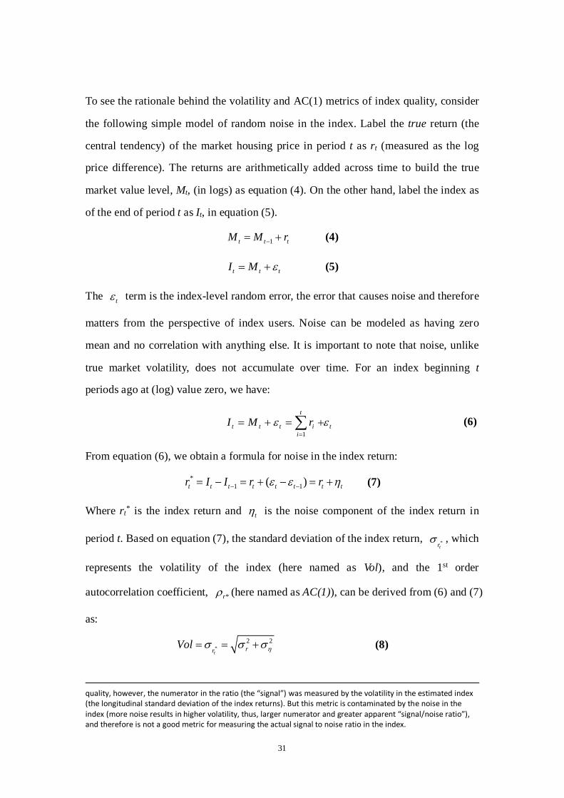
To see the rationale behind the volatility and AC(1) metrics of index quality, consider

the following simple model of random noise in the index. Label the true return (the

central tendency) of the market housing price in period t as rt (measured as the log

price difference). The returns are arithmetically added across time to build the true

market value level, Mt, (in logs) as equation (4). On the other hand, label the index as

of the end of period t as It, in equation (5).

(4)

(5)

The term is the index-level random error, the error that causes noise and therefore

matters from the perspective of index users. Noise can be modeled as having zero

mean and no correlation with anything else. It is important to note that noise, unlike

true market volatility, does not accumulate over time. For an index beginning t

periods ago at (log) value zero, we have:

t

t

iittt rMI εε ∑

=

+=+=1

(6)

From equation (6), we obtain a formula for noise in the index return:

(7)

Where rt* is the index return and is the noise component of the index return in

period t. Based on equation (7), the standard deviation of the index return, , which

represents the volatility of the index (here named as Vol), and the 1st order

autocorrelation coefficient, (here named as AC(1)), can be derived from (6) and (7)

as:

(8)

quality, however, the numerator in the ratio (the “signal”) was measured by the volatility in the estimated index (the longitudinal standard deviation of the index returns). But this metric is contaminated by the noise in the index (more noise results in higher volatility, thus, larger numerator and greater apparent “signal/noise ratio”), and therefore is not a good metric for measuring the actual signal to noise ratio in the index.

1t t tM M r−= +

t t tI M ε= +

tε

*1 1( )t t t t t t t tr I I r rε ε η− −= − = + − = +

tη

*tr

σ

*rρ

*2 2

trr

Vol ησ σ σ= = +

31

(9)

Where and are the variance of the true return and the noise respectively,

and is the 1st order autocorrelation coefficient of the true return (which is

normally positive in real asset markets).31

Volatility is dispersion in returns over time. There is always true volatility in that the

actual true market prices evolve and change over time. The ideal price index filters

out the noise-induced volatility to leave only the true market volatility. The noise

(random error) in the index adds to volatility in the index, beyond and in addition to

the true volatility. So, noise causes excess or erroneous volatility in the index. This

excess volatility brings down the 1st order autocorrelation, as pure noise has an AC(1)

value of negative 50%.32 In Equation (8), smaller means less noise, lower index

volatility and a better estimation of market return each period. Thus, smaller Vol or

higher AC(1) will indicate a better quality housing price index in the sense of a less

noisy index.33

We calculate these two statistics for each of the indices we have estimated in Figure 3.

The results are shown in the first two rows in Table 4. We can see that the volatility

measures of the three ps-RS indices are much lower than that of the hedonic index.

The ps-RS indices also have much higher first order autocorrelation coefficients than

the hedonic index.34 Among the three ps-RS indices, the building-based version has

31 Note that is a longitudinal moment (dispersion in market returns across time), while is a cross-sectional moment (dispersion across index return estimation error as of each point in time). 32 With = 0, equation (9) gives: ρr* = -1/2. 33 Note that this indication of the volatility and AC(1) metrics is within the context of the concern about random error in the index, in which lower volatility and higher AC(1) indicates less error. It is possible, however, that sources of systematic bias error could also cause low volatility and/or high AC(1). Such an effect has been noted, for example, in studies of appraisal-based indices of commercial property prices. Broader considerations and analyses are required to distinguish such bias effects from a lack of noise. In the present context, the discussion in the preceding section 5.2 addressed the issue of systematic bias. 34 The specific values of the AC(1) metric can also tell us something about the quality of a real estate price index. As noted, ample evidence suggests that in private search markets that trade unique, whole assets, prices do not follow a Random Walk as is typical of prices of stocks traded in public stock exchanges. Rather, asset prices in private search markets tend to have inertia over short to medium time intervals, leading to positive AC(1) in the

2 2 2 2*(1) ( / 2) / ( )r r r rAC η ηρ ρ σ σ σ σ= = − +

2rσ

2ησ

rρ

2ησ

2rσ

2ησ

2rσ

32

the lowest volatility and the highest first order autocorrelation. These results suggest

that the ps-RS has less noise than the hedonic, and the smaller the matching space is,

the better performance in terms of noise reduction. Presumably this is due to the

building-based ps-RS index controlling better for the variation in housing

characteristics, given a sample size that is, even in the building-based index, more

than sufficient to mitigate purely random estimation error. This conclusion is also

suggested perhaps more compellingly by a simple visual comparison of the indices in

Figure 3. The ps-RS indices are noticeably smoother than the hedonic.

*** Insert Table 4 about here ***

The third test we use for index quality in terms of minimizing random error is based

on the Hodrick & Prescott filter (HP filter). 35 In some sense this is a formal

quantification of the “eyeball test” of the visual smoothness of the index in a graph.

The HP filter has been promoted by Hodrick and Prescott (1997) in order to analyze

time series data. It is a spline fitting method that divides a time series into two smooth

components, a secular trend and a cyclical component. The HP filter has been

popularly used to analyze macroeconomic variables as well as price series in real

estate markets (Cocconcelli and Medda, 2013). In STATA 12.0, we separate the trend

and cyclic series for all of our target indices in Figure 7: building-version,

phase-version, and complex-version ps-RS indices, and the hedonic index. The

smoothed trend-and-cyclical versions of the four indices are shown in Figure 7 (solid

lines). The HP-based comparison of the indices is essentially a quantification of

smoothness. We want to see which index has the least deviation from its smoothed HP

representation. We compute the index returns and the smoothed returns of the

corresponding HP representation. For each type of index we compute the sum of

squared differences between the index returns and its smoothed returns across the

history, and then we compare these sums. The results are shown in the bottom row in

returns, whereas a Random Walk has AC(1) = 0. A finding of negative AC(1), such as indicated in Table 4 for the hedonic index, would generally from an a prori perspective be indicative of random estimation error in the price index. 35 We thank Albert Saiz for suggesting this test.

33

Table 4. Once again, the building-based version of the ps-RS index comes out looking

best, with the smallest deviation from its smoothed representation. This is also

consistent with our findings from the AC(1) and volatility tests which are also

reported in Table 4.

*** Insert Figure 7 about here ***

We also calculate these three noise indicators for the building-version ps-RS indices

with different similarity thresholds for the pseudo-pair matching construction

procedure (Table 5). As noted in section 5.2.2, the choice of the threshold is a

trade-off between the within-pair “similarity” (higher similarity is good for mitigating

bias) and the sample size (larger size is good for reducing random errors). Therefore

our expectation is that the ps-RS index with stricter similarity threshold will have

more noise embodied in the index, and thus have larger volatility, smaller AC(1) and

larger sum of the square of deviations of return. The indicators in Table 5 do show

these patterns, though the differences are not very big, reflecting the fact that the

Chengdu transaction sample is quite large at the metro-wide aggregate level.

*** Insert Table 5 about here ***

5.3.2 Out-of-sample robustness check

Though related to the noise tests, out-of-sample prediction tests offer another

perspective on the reliability and robustness of the index estimation. To conduct this

test, we randomly divide the whole sample into two sub-samples, independently

estimate the index based on each of the sub-samples separately, and compare the

resulting indices. We do this four different ways according to the sizes of the two

sub-samples. We examine 20% vs. 80% (of the whole sample), 30% vs. 70%, 40% vs.

60% and 50% vs. 50%, respectively.36 For each subsample pair, we estimate two

36 We assign a uniform-distributed random number between 0 and 1 to each observation using the command “runiform” in STATA. We then assign the observations with this random number less than a threshold (such as 0.2,

34

separate ps-RS indices for the two subsamples, in all cases building-based with no

distance metric threshold. The two indices in any pair are almost the same (no

visually apparent difference at all, as shown in Figure 8) with high cross-correlation

coefficients in the returns: above 0.999.

Furthermore, we conduct mean-comparison tests between the two indices in each

subsample pair with the null hypothesis as H0: , where t

indicates the period number. The t-value of the test for the 50% vs. 50% subsample

pair is only 0.015 and the p-value is as high as 0.988, which indicates that statistically

we are not even close to being able to reject the H0, implying that the two indices

based on randomly constructed two 50% sub-samples are statistically

indistinguishable from each other. The t-values and p-values of the other subsample

pairs are shown at the bottom of Figure 8, which also cannot reject the H0.

*** Insert Figure 8 about here ***

6. Conclusion

The traditional same-property repeat sales model can be regarded as an extreme case

of a matching rule, pairing only sales of the exact same house. We develop a pseudo

repeat sales (ps-RS) model that is appropriate in those residential markets in many

rapidly-growing high-density cities where each residential complex typically contains

several phases, a number of buildings, and hundreds or even thousands of nearly

homogeneous housing units sharing the same location and neighborhood attributes.

We generate within-complex, within-phase, and within-building pairs, respectively.

By regressing the within-pair price differentials onto the classical RS time-dummies

and the relatively small and easily observed within-pair differentials in the housing

units’ physical attributes (the more problematical observed and unobserved hedonic

variables are cancelled out), we are able to construct three versions of ps-RS price

0.3, 0.4 and 0.5), to the first sub-sample and the others to the second sub-sample.

1, 2,( ) 0t tmean Index Index− =

35

indices for new homes, with complex, phase and building as matching spaces,

respectively. These new ps-RS indices show good results in mitigating the problem of

omitted variables which can bias hedonic index estimation. In particular, the

building-version ps-RS index does the best job in this regard because its within-pair

differential is the smallest, and we see empirically that this index displays noticeably

less long-term price appreciation than indices that do not control as well for

unobservable hedonic differences (including omitted variables in the hedonic index).

For the building-version ps-RS model, we further introduce a flexible distance metric

criterion based on the absolute value of the within-pair difference of the predicted

hedonic values. By setting this criterion one can deal explicitly and flexibly with the

trade-off between the “purity” of the within-pair hedonic attribute homogeneity

(which can cause bias in the index) and the estimation sample size that can mitigate

random error or noise in the index. Our ps-RS index also addresses the problems of

the classical repeat sales index regarding sample size and sample selection bias, as it

uses all available sales transactions. Furthermore, by actually increasing the effective

estimation sample size through the sale-pairing process, the ps-RS model results in

very smooth, precise, and reliable indices. And it provides a parsimonious, simpler,

more transparent and easily understood specification that is more robust to data issues

and more tailored to application in the real world of the Chinese context or other such

rapidly urbanizing countries, possibly lending itself particularly well to regularly

published “official” price tracking index production.

We estimate both the ps-RS indices and a comparable hedonic index using a

large-scale new home transaction dataset in Chengdu. The two types of indices show

very similar trend and turning points. The complex-based version of the ps-RS index

parallels the hedonic index, suggesting that the hedonic index is not superior to the

ps-RS index in terms of systematic results, while the ps-RS is simpler and more

robust and provides a smoother index more free of noise. The phase-based version of

the ps-RS index has a lower growth trend, and the building-based version shows the

lowest price growth of all. From these results we infer that omitted or poorly

36

measured location attributes do not have much net effect on a hedonic index in

Chengdu, but omitted or poorly measured physical quality attributes tend to cause an

upward bias in the price growth trend of the hedonic index (and of the complex-based

ps-RS index). Building-based ps-RS indices with different distance metric thresholds

are almost the same with very tiny eye-balling differences. Furthermore, the ps-RS

indices have better performance than the hedonic index in tests for random error or

estimation reliability, as indicated by out-of-sample prediction and tests of

smoothness or signal-to-noise ratio. We explicate and demonstrate formal

signal-to-noise oriented metrics of index quality in terms of minimizing random

estimation error.In summary, the ps-RS would seem to be an important new real estate

price index methodology contribution particularly appropriate for rapidly urbanizing

economies with high-density cities, such as in mainland China, Taiwan, Singapore

and many other Asian cities (and in the future probably in South Asia and Africa).

Recently the National Bureau of Statistics of China has been collecting micro housing

transaction data (instead of relying on developers’ self-reported numbers) and trying

to develop a more reliable and also practical price index construction methodology.

The ps-RS method may warrant serious consideration.

Acknowledgements: Siqi Zheng is supported in part by the National Natural Science Foundation

of China under Grant 71322307, 70973065 and 71273154, by the Program for New Century

Excellent Talents in University (NCET-12-0313) and by the Tsinghua University Initiative

Scientific Research Program. Hongyu Chen and Yaoguo Wu provided excellent research

assistance. The authors appreciate the suggestions of Albert Saiz, Marc Francke, and an

anonymous referee, as well as participants in the National University of Singapore Department of

Real Estate Seminar in August, 2012.

Reference

[1] Bailey M J, Muth R F, Nourse H O. A regression method for real estate price index

construction[J]. Journal of the American Statistical Association, 1963, 58(304): 933-942.

37

[2] Bokhari S, Geltner D. Estimating real estate price movements for high frequency tradable

indexes in a scarce data environment[J]. The Journal of Real Estate Finance and Economics,

2012, 45:522-543.

[3] Case B, Pollakowski H O, Wachter S M. On choosing among house price index

methodologies[J]. Real estate economics, 1991, 19(3): 286-307.

[4] Case B, Quigley J M. The dynamics of real estate prices[J]. The Review of Economics and

Statistics, 1991: 50-58.

[5] Case K E, Shiller R J. The efficiency of the market for single-family homes[J]. 1989.

[6] Case K E, Shiller R J. Prices of single family homes since 1970: New indexes for four

cities[J]. 1987.

[7] Chen Y, John M C, Dogan T. Hedonic estimation of housing demand elasticity with a markup

over marginal costs [J]. Journal of Housing Economics, 2011, 20(4): 233-248.

[8] Clapp J, Giacotto C. Estimating price indices for residential property: A comparison of repeat

sales and assessed value methods [J]. Journal of the American Statistical Association, 1992,

87: 300-306.

[9] Cocconcelli L, Medda F. Boom and bust in the Estonian real estate market and the role of

land tax as a buffer [J]. Land Use Policy, 2013: 30, 392-400.

[10] Court A. Hedonic price indices with automotive examples [J]. The Dynamics of Automobile

Demand, 1939, General Motors Corporation.

[1] Deng Y, Mcmillen D P, Sing T F. Private residential price indices in Singapore: A matching

approach[J]. Regional Science and Urban Economics, 2011.

[12] Englund P, Quigley J M, Redfearn C L. The choice of methodology for computing housing

price indexes: comparisons of temporal aggregation and sample definition[J]. The journal of

real estate finance and economics, 1999, 19(2): 91-112.

[13] M.Francke. Repeat Sales Index for Thin Markets: A Structural Time Series Approach [J].

Journal of Real Estate Finance & Economics, 2010, 41: 24-52.

[14] Fu Y, Tse D K, Zhou N. Housing choice behavior of urban workers in China's transition to a

housing market[J]. Journal of Urban Economics, 2000, 47(1): 61-87.

[15] Gatzlaff D H, Haurin D R. Sample selection and biases in local house value indices[J].

Journal of Urban Economics, 1998, 43(2): 199-222.

38

[16] Geltner, D. "Bias & Precision of Estimates of Housing Investment Risk Based on

Repeat-Sales Indexes: A Simulation Analysis", Journal of Real Estate Finance & Economics,

14(1/2): 155-172, January/March 1997

[17] Geltner D, Pollakowski H. On the Magnitude of Noise in the Moody's/REAL Index Return

Reports, MIT Center for Real Estate-CREDL, 2008.

[18] Glendinning M, Muthesius S, Paul M C F S. Tower Block: Modern Public Housing in

England, Scotland, Wales, and Northern Ireland[M]. Paul Mellon Centre for Studies in

British Art, 1994.

[19] Griliches Z, Adelman I. On an index of quality change [J]. Journal of the American Statistical

Association, 1961, 56:295, 535-548.

[20] Hansen J. Australian House Prices: A Comparison of Hedonic and Repeat ‐Sales

Measures*[J]. Economic Record, 2009, 85(269): 132-145.

[21] Hodrick R, Prescott E. Postwar U.S. Business Cycles: An Empirical Investigation[J]. Journal

of Money, Credit and Banking, 1997, 29:1, 1-16.

[22] Kain J F, Quigley J M. Measuring the value of housing quality[J]. Journal of the American

Statistical Association, 1970: 532-548.

[23] Mcmillen D P. Price indices across the distribution of sales prices: A matching approach[J].

Urbana, 2010, 51: 61801.

[24] McMillen D P. Repeat Sales as a Matching Estimator [J]. Real Estate Economics, 2012:

745-772.

[25] McMillen D P, Dombrow J. A Flexible Fourier Approach to Repeat Sales Price Indexes [J].

Real Estate Economics, 2001: 207-225.

[26] Peláez R. The housing bubble in real-time: the end of innocence [J]. Journal of Economics

Finance, 2012: 36, 211-225.

[27] Quigley J M. A simple hybrid model for estimating real estate price indexes[J]. Journal of

Housing Economics, 1995, 4(1): 1-12.

[28] Rosen S. Hedonic rrices and implicit markets: product differentiation in pure competition [J].

Journal of Political Economy, 1974, 82:1, 34-55.

[29] Shiller R. Macro Markets: Creating Institutions for Managing Society’s Greatest Risks [M].

Oxford: Clarendon Press, 1993.

39

[30] Wallace N E, Meese R A. The construction of residential housing price indices: a comparison

of repeat-sales, hedonic-regression, and hybrid approaches[J]. The Journal of Real Estate

Finance and Economics, 1997, 14(1): 51-73.

[31] Zheng S, Fu Y, Liu H. Housing-choice hindrances and urban spatial structure: Evidence from

matched location and location-preference data in Chinese cities[J]. Journal of Urban

Economics, 2006, 60(3): 535-557.

40

Figure 1 Matching Process across Periods within a Matching Space (Building,

Phase, or Complex)

Period 1 Period 2 Period 3 Period 4

3 X 2=6 2 X 3=6

41

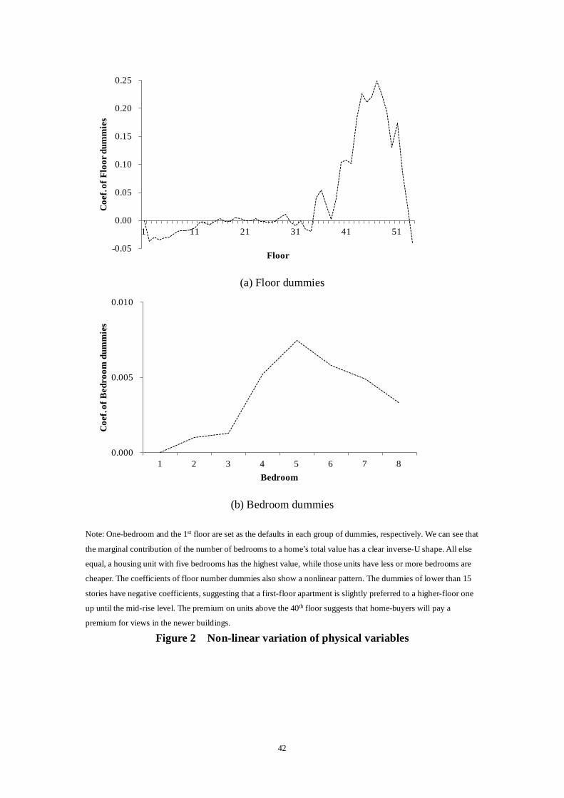
(a) Floor dummies

(b) Bedroom dummies

Note: One-bedroom and the 1st floor are set as the defaults in each group of dummies, respectively. We can see that

the marginal contribution of the number of bedrooms to a home’s total value has a clear inverse-U shape. All else

equal, a housing unit with five bedrooms has the highest value, while those units have less or more bedrooms are

cheaper. The coefficients of floor number dummies also show a nonlinear pattern. The dummies of lower than 15

stories have negative coefficients, suggesting that a first-floor apartment is slightly preferred to a higher-floor one

up until the mid-rise level. The premium on units above the 40th floor suggests that home-buyers will pay a

premium for views in the newer buildings.

Figure 2 Non-linear variation of physical variables

-0.05

0.00

0.05

0.10

0.15

0.20

0.25

1 11 21 31 41 51

Coe

f. of

Flo

or d

umm

ies

Floor

0.000

0.005

0.010

1 2 3 4 5 6 7 8

Coe

f. of

Bed

room

dum

mie

s

Bedroom

42

Note: Three sorts of ps-RS indices with different matching spaces are shown with the standard Hedonic index.

Besides, in order to make an apples-to-apples comparison between the ps-RS index and the standard hedonic index,

we employ weighted least squares (WLS) to estimate a new complex-based ps-RS index whose hedonic attribute

weights over time will be the same as those in the hedonic index. The OLS and WLS complex-based indices are

almost the same, suggesting that hedonic attribute drift effects are not importantly different between the hedonic

and the ps-RS indices.

Figure 3 Three ps-RS Indices and the Hedonic Index for Chengdu

1

1.5

2

2.5

Jan-06 Jan-07 Jan-08 Jan-09 Jan-10 Jan-11

by_Cmplx

by_Lcns

by_Bldg

Hedonic_zone

by_Cmlx_weighted

43

Figure 4 Comparison of ps-RS index and NBSC index

100

125

150

Mar-09 Sep-09 Mar-10 Sep-10 Mar-11 Sep-11

ps-RS Index

NBSC Index

44

Note: the distribution of the “hedonic value” distance metric (in logarithm) of all the pairs generated in the

building version ps-RS model. We can see the sharp decreasing number of pairs as the distance metric increases.

This reflects the fact that most units tend to be very similar within a building.

Figure 5 Distribution of the distance metric threshold

02

46

8D

ensi

ty

0 .5 1 1.5 2 2.5D ista nce M etric

45

Note: Given the hedonic-value-distance distribution, we pick up several subsamples under different distance metric

thresholds: the 100% (full sample), the 60% and the 20% (most homogeneous) subsamples, and the subsample that

uses only the single pair with the smallest distance metric (similar to McMillen, 2012). The sample size shrinks

significantly from 14.4 million pairs, to 8.7 million, 2.9 million and 0.11 million pairs respectively. The result

indicates that setting different distance metric thresholds does not influence the trend and cyclical patterns of the

index. However, the larger sample size based on the looser similarity threshold does appear to noticeably reduce

the excess volatility.

Figure 6 Comparison of building version ps-RS indices with different distance

metric thresholds

1

1.5

2

Jan-06 Jul-06 Jan-07 Jul-07 Jan-08 Jul-08 Jan-09 Jul-09 Jan-10 Jul-10 Jan-11 Jul-11

All sample (14,388,523 obs.)

60% sample (8,656,337 obs.)

20% sample (2,904,147 obs.)

Smallest distance metric (114,291 obs., 0.79%)

46

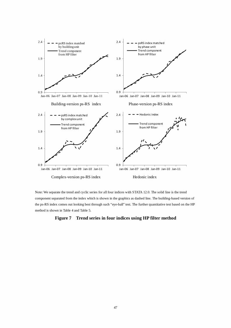
Building-version ps-RS index Phase-version ps-RS index

Complex-version ps-RS index Hedonic index

Note: We separate the trend and cyclic series for all four indices with STATA 12.0. The solid line is the trend

component separated from the index which is shown in the graphics as dashed line. The building-based version of

the ps-RS index comes out looking best through such “eye-ball” test. The further quantitative test based on the HP

method is shown in Table 4 and Table 5.

Figure 7 Trend series in four indices using HP filter method

0.9

1.4

1.9

2.4

Jan-06 Jan-07 Jan-08 Jan-09 Jan-10 Jan-11

psRS index matched by building unitTrend component from HP filter

0.9

1.4

1.9

2.4

Jan-06 Jan-07 Jan-08 Jan-09 Jan-10 Jan-11

psRS index matched by phase unitTrend component from HP filter

0.9

1.4

1.9

2.4

Jan-06 Jan-07 Jan-08 Jan-09 Jan-10 Jan-11

psRS index matched by complex unit

Trend component from HP filter

0.9

1.4

1.9

2.4

Jan-06 Jan-07 Jan-08 Jan-09 Jan-10 Jan-11

Hedonic index

Trend component from HP filter

47

(a) 50%-50% pair

(b) 20%-80% pair

Figure 8 Out-of-Sample Robustness Check

1

1.5

2

Jan-06 Jan-07 Jan-08 Jan-09 Jan-10 Jan-11 Jan-12

50% random sample

other 50% sample

Correlation: 0.999993Root MSE (50%): 0.08969t-value: 0.015, p-value: 0.988

1

1.5

2

Jan-06 Jan-07 Jan-08 Jan-09 Jan-10 Jan-11 Jan-12

20% random sample

other 80% sample

Correlation: 0.999898Root MSE (20%): 0.08975Root MSE (80%): 0.08966t-value:0.028, p-value: 0.937

48

Table 1 Variable Definition and Descriptive Statistics

Variables Unit Description Mean Median Max Min Sd.Dev

Physical Attributes

PRICE million RMB

Yuan Total purchase price 0.57 0.51 3.49 0.06 0.29

SIZE square meter Housing unit size 97.64 89.25 282.68 14.79 30.63

FLOOR / Floor number 12.43 11.00 54.00 1.00 7.96

BEDROOM / Number of bed rooms 2.22 2.00 8.00 1.00 0.77

TFLOOR / Building height (stories) 23.73 22.00 66.00 3.00 8.19

Location Attributes

D_CBD km Distance to city center 6.95 6.50 36.01 0.26 3.09

ZONE dummy 33 zones

49

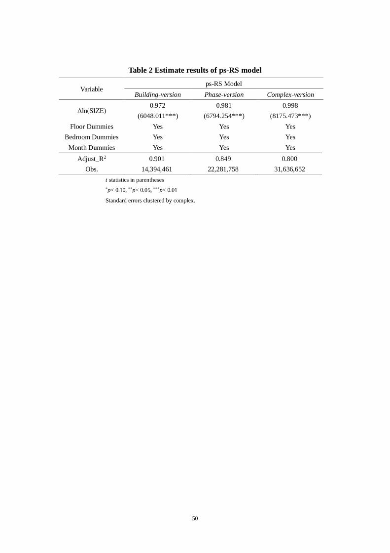
Table 2 Estimate results of ps-RS model

Variable ps-RS Model

Building-version Phase-version Complex-version

Δln(SIZE) 0.972

(6048.011***) 0.981

(6794.254***) 0.998

(8175.473***) Floor Dummies Yes Yes Yes

Bedroom Dummies Yes Yes Yes Month Dummies Yes Yes Yes

Adjust_R2 0.901 0.849 0.800 Obs. 14,394,461 22,281,758 31,636,652

t statistics in parentheses *p< 0.10, **p< 0.05, ***p< 0.01

Standard errors clustered by complex.

50

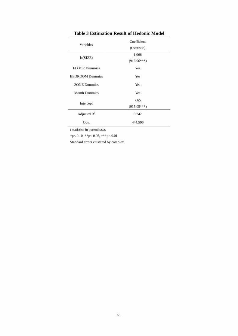
Table 3 Estimation Result of Hedonic Model

Variables Coefficient

(t-statistic)

ln(SIZE) 1.066

(916.96***)

FLOOR Dummies Yes

BEDROOM Dummies Yes

ZONE Dummies Yes

Month Dummies Yes

Intercept 7.65

(915.05***)

Adjusted R2 0.742

Obs. 444,596

t statistics in parentheses

*p< 0.10, **p< 0.05, ***p< 0.01

Standard errors clustered by complex.

51

Table 4: Comparing Index Smoothness: Three Metrics: Volatility, First-Order Autocorrelation, and Sum of Squared

Differences Between Index and its Hodrick-Prescott Representation

Building-version

Ps-RS License-version

Ps-RS Complex-version

Ps-RS Hedonic

Volatility 0.016 0.023 0.034 0.080

AC(1) 0.599 0.405 0.256 -0.094

sum of the square of deviations of return

0.006 0.011 0.022 0.122

52

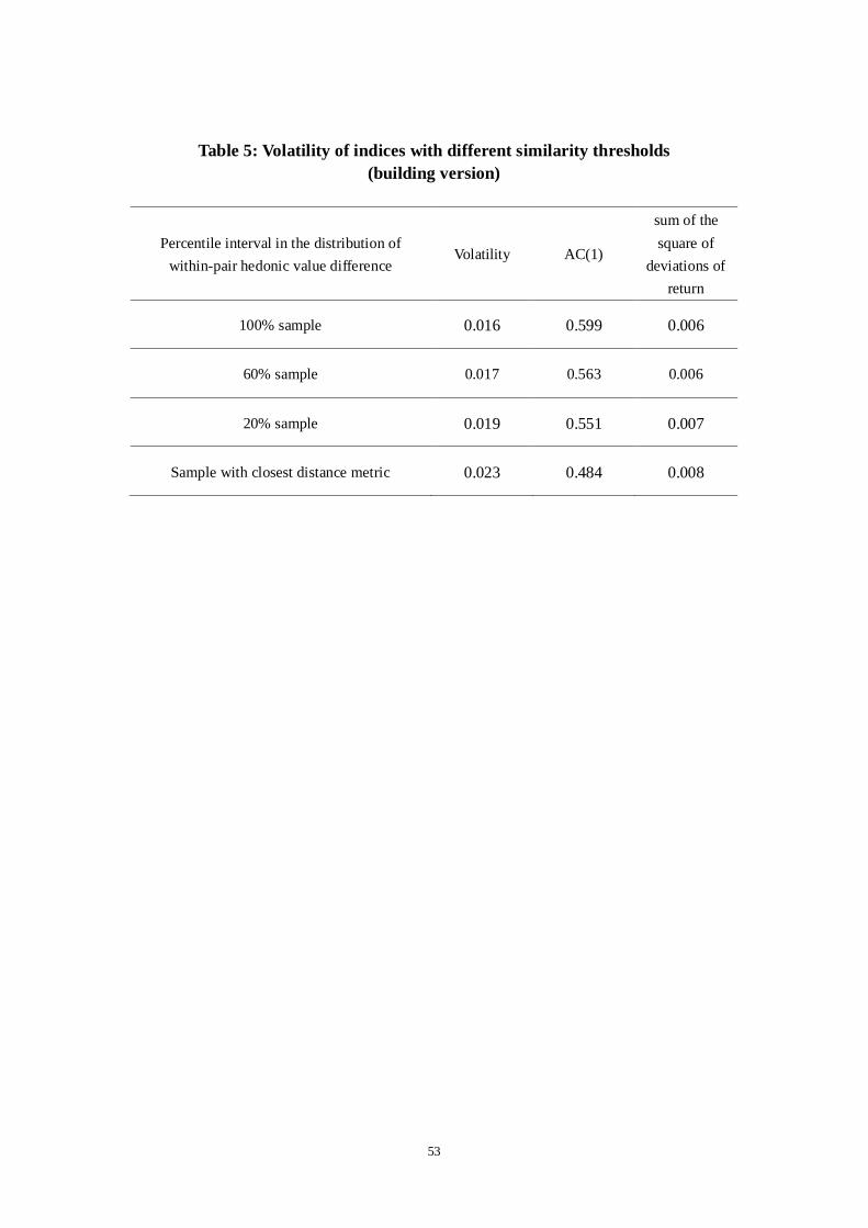
Table 5: Volatility of indices with different similarity thresholds (building version)

Percentile interval in the distribution of within-pair hedonic value difference

Volatility AC(1)

sum of the square of

deviations of return

100% sample 0.016 0.599 0.006

60% sample 0.017 0.563 0.006

20% sample 0.019 0.551 0.007

Sample with closest distance metric 0.023 0.484 0.008

53