a modeling approach for hvac systems based on...

A Modeling Approach for HVAC Systemsbased on the LoLiMoT Algorithm

Jakob Rehrl ∗ Daniel Schwingshackl † Martin Horn ∗

∗ Institute of Automation and Control, Graz University of Technologye-mail: [email protected]

† Control and Mechatronic Systems Group, Institute of SmartSystem-Technologies, Alpen-Adria-Universitat Klagenfurt

Abstract: In heating ventilating and air conditioning (HVAC) systems, typically two variables(air temperature and air humidity) have to be controlled via several (at least two) actuators.Some of the components show nonlinear behaviour. Therefore, HVAC systems belong to theclass of nonlinear multi-input-multi-output systems. A well suited approach to control this classof systems is model predictive control, since the time constants of HVAC systems are high(typically in the range of tens or hundreds of seconds) offering enough time to perform therequired online optimization. In order to apply linear predictive control methods, while takinginto account the nonlinearities of the plant, a modeling concept based on a physical plant modeland a neuro-fuzzy model is proposed. The neuro-fuzzy model is obtained via the so called locallinear model tree (LoLiMoT) algorithm. The generation of a linear state space representationfrom the neuro-fuzzy model is demonstrated. This linear state space model can then be used ina predicitive control scheme, where the linear model is updated each sampling instant from theneuro-fuzzy model. This technique allows the application of standard linear predictive controlwhile taking into account the nonlinearities of the plant. Simulation and measurement resultsobtained from an industrial test plant are presented.

1. INTRODUCTION

The operation of heating, ventilating and air conditioning(HVAC) systems requires the compliance with demandingspecifications concerning control accuracy of air temper-ature and air humidity. The applied control technique isa crucial factor influencing the performance of the overallsystem. Therefore, appropriate control techniques have tobe developed. Typical system properties as well as state-of-the-art approaches to control HVAC systems are presentedin the following.

A common problem setup is the simultaneous control ofair temperature and humidity via the following actuators:Heating and cooling coils are used to control the air tem-perature. These components are realized as finned tubecrossflow heat exchangers. For humidity control, steamhumidifiers and cooling coils are used. All these actuatorsinfluence both humidity and temperature, i.e. the givensetup describes a multi-input-multi-output (MIMO) con-trol problem. Furthermore, the relative humidity is a non-linear function of the temperature and some componentswithin HVAC systems show nonlinear behaviour. E.g., themixing ratio of hot water and return water of the heatingcoil is a nonlinear function of the valve position.

In the field of HVAC control systems, there exist ap-proaches that take into account the MIMO property ofthe plant. In Anderson et al. [2008, 2007], an experimentalsmall scale HVAC system is presented. The authors designan H∞ controller for the simultaneous control of dischargeair temperature and air flow rate. A linearized plant modelincluding dead times is proposed, nonlinearities are re-

garded as model uncertainties. Humidity is not consideredat all. In Semsar-Kazerooni et al. [2008] nonlinear meth-ods are applied to control thermal space and supply airtemperatures. The system model is a bilinear system. Theproposed concept demonstrates the potential of nonlinearcontrol techniques for HVAC systems in simulation stud-ies. Again, humidity is neglected. Many recent works pro-pose model predictive control (MPC) strategies to controlHVAC systems, see Aswani et al. [2012b], Kelman andBorrelli [2011], Aswani et al. [2012a], Naidu and Rieger[2011], Huang and Wang [2008]. In Rehrl and Horn [2011],MPC in combination with exact linearization is appliedto the outlet air temperature control of a cooling coil.Actuator saturation cannot be taken into account directlydue to the application of the exact linearization method,see e.g. Isidori [1995].

Due to the following reasons, MPC is well suited for theapplication in HVAC systems:

• The method is directly applicable to MIMO systems.• Dead times can be handled easily.• The sampling time of the considered class of systems

is in the range of 10 seconds. Therefore, it is possibleto solve the online optimization problem in time withstandard computer hardware 1 .

The use of a nonlinear plant model within the MPCincreases the complexity to solve the online optimizationproblem considerably (e.g. local minima). The non-convex

1 The presented test plant is equipped with a X20-System witha 650 MHz Celeron PLC from B&R automation (http://www.br-automation.com).

Preprints of the 19th World CongressThe International Federation of Automatic ControlCape Town, South Africa. August 24-29, 2014

Copyright © 2014 IFAC 10862

optimization problem is solved via evolutionary program-ming (EP) in Jalili-Kharaajoo [2005]. However, in EP it isnot guaranteed that the found minimum is a global one.In Kelman and Borrelli [2011], Ma et al. [2012] MPC issuggested in order to minimize the energy consumptionof HVAC systems. Sequential quadratic programming isapplied to solve the optimization problem. It is statedthat the computational complexity to solve the low-level,non-convex, MPC problem causes problems with standardHVAC controller hardware.

Consequently, in this paper, a modeling approach fornonlinear MIMO systems is presented and demonstratedin HVAC systems. The proposed model can easily beapplied in linear MPC, while still taking into accountthe nonlinear plant characteristics. The suggested strategyrelies on a linear plant model which is generated from anonlinear system representation at each sampling instant,see Section 4. This linear model is used for the onlineMPC problem to compute the predicted trajectory ofthe system state. At the next time step, a new linearmodel is generated (from the actual system state) whichis then again used for prediction. Of course, the linearsystem is an approximation, however, the accuracy of theapproximation is increased by updating the model eachtime step. A detailed explanation of the two models isgiven in Section 3.

This paper focuses on the modeling of the plant and thegeneration of the linear plant model. It is structured asfollows: Section 2 gives a description of the test plant whichis used to verify the proposed modeling approach. Section 3deals with the modeling of the plant and the motivationfor the application of the proposed approach can befound there. A mathematical model of the consideredHVAC system based on physical relations is presented.Furthermore, a neuro-fuzzy model is given to representthe plant dynamics. In Section 4 the computation of astate space model from the neuro-fuzzy model is presented.Section 5 shows the application of the method for modelinga system with two inputs (heating coil power and steamhumidifier power) and two outputs (air temperature andair humidity). Section 6 concludes the paper and outlinesfuture work.

2. PLANT

The considered plant is an industrial HVAC system shownin Fig. 1. The white arrows indicate possible air paths:outer air enters the plant from the right, room air entersfrom the top right hand corner. The conditioned aircan be transported into the room or via an air duct tothe neighboring factory building. In the problem setupdescribed in the present paper, one heating coil will beused to increase the air temperature, whereas the steamhumidifier is used to increase the air humidity.

3. MODELING

In the following, two types of plant models will be pre-sented: a detailed physically motivated model that formsthe basis for simulation studies as well as a local linearneuro-fuzzy model created via the so-called local linearmodel tree (LoLiMoT) algorithm, see e.g. Nelles [2010,

1997]. These models will be referred to as “physical model”and “LoLiMoT model” respectively in the following. Theuse of these two types of models is motivated by thefollowing reasons:

• The LoLiMoT model offers the opportunity to extracta linear time invariant (LTI) system model in astraightforward way (see Section 4). For the givenphysical model, the direct computation of linearizedmodels is difficult for the following reason: Due tothe segmentation of the heating and cooling coils(see Section 3.1.1), there are numerous state variablesthat are not measurable. The design of an observerfor the nonlinear physical plant model with typically(depending on the number of segments) hundredsof state variables would be a non-trivial task. Inorder to use the linearized model in a control scheme,the system order should not be that high, i.e. orderreduction techniques would be required, whereas theLoLiMoT approach can yield sufficiently good resultswith local model orders of one, see Schwingshacklet al. [2013]. These arguments justify the use of theLoLiMoT model. The LTI model extracted from theLoLiMoT model will serve as basis for the applicationin a linear MPC control strategy.

• To identify the LoLiMoT model parameters, all in-puts (actuating signals and measurable disturbances)have to be excited properly. Some of the disturbancescannot be excited as they are prescribed by, e.g., out-door air conditions in the real world system. There-fore, the mentioned physical model is used to generatethe identification signals for the LoLiMoT model.

• The parameters of the physical model are knownfrom geometry data of the components as well asfrom material properties. Only few parameters (e.g.heat transfer coefficient, time constants of tempera-ture sensors) are identified from measured data. Toidentify them, the excitation of the real world systemvia the actuators is sufficient.

In the following subsections, the physical as well as theLoLiMoT model will be described. A notation describingthe variables can be found in the appendix.

3.1 Physical Model

The model of the complete plant is obtained by intercon-necting single component models. The core componentsare the following:

• Heating coils / cooling coils• Hydraulic system for the heating and cooling coils• Steam humidifier• Temperature and humidity sensors

Fig. 2 shows a schematic representation of the relevantplant components. Plant inputs are the actuating signalsu1 and u2 of heating coil and humidifier, as well asthe disturbances d1 (air inlet temperature) and d2 (hotwater supply temperature). Supply air temperature y1 andsupply air humidity y2 represent the controlled variables.In the following, descriptions as well as mathematicalmodels of the mentioned components are presented.

Heating/Cooling Coil Both, heating and cooling coil arerealized as so-called finned tube, crossflow heat exchanger.

19th IFAC World CongressCape Town, South Africa. August 24-29, 2014

10863

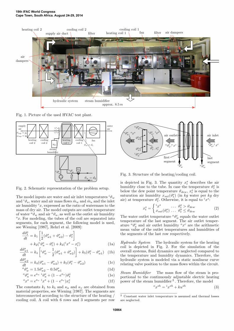
Fig. 1. Picture of the used HVAC test plant.

Fig. 2. Schematic representation of the problem setup.

The model inputs are water and air inlet temperatures iϑwand iϑa, water and air mass flows mw and ma and the inletair humidity ix, expressed as the ratio of watermass to themass of dry air. The model outputs are outlet temperatureof water oϑw and air oϑa, as well as the outlet air humidityox. For modeling, the tubes of the coil are separated intosegments, for each segment, the following model is used,see Wiening [1987], Rehrl et al. [2009]:

dϑstdt

= k1

[1

2(ϑsw1 + ϑsw2)− ϑst

]+ k2(iϑsa − ϑst ) + k3(ixs − xst ) (1a)

dϑsw1

dt= k4

[iϑsw −

1

2(ϑsw1 + ϑsw2)

]+ k5(ϑst − ϑsw1) (1b)

dϑsw2

dt= k4(ϑsw1 − ϑsw2) + k5(ϑst − ϑsw2) (1c)

oϑsw = 1.5ϑsw2 − 0.5ϑsw1 (1d)oϑsa = eκa iϑsa + (1− eκa)ϑst (1e)oxs = eκv ixs + (1− eκv )xst (1f)

The constants k1 to k5 and κa and κv are obtained frommaterial properties, see Wiening [1987]. The segments areinterconnected according to the structure of the heating /cooling coil. A coil with 6 rows and 3 segments per row

Fig. 3. Structure of the heating/cooling coil.

is depicted in Fig. 3. The quantity xst describes the airhumidity close to the tube. In case the temperature ϑst isbelow the dew point temperature ϑdew, xst is equal to thesaturation air humidity xsat(ϑ

st ) (in kg water per kg dry

air) at temperature ϑst . Otherwise, it is equal to ixs:

xst =

{ixs . . . ϑst > ϑdewxsat(ϑ

st ) . . . ϑ

st ≤ ϑdew

(2)

The water outlet temperature oϑcw equals the water outlettemperature of the last segment. The air outlet temper-ature oϑca and air outlet humidity oxc are the arithmeticmean value of the outlet temperatures and humidities ofthe segments of the last row respectively.

Hydraulic System The hydraulic system for the heatingcoil is depicted in Fig. 2. For the simulation of theoverall systems, fluid dynamics are neglected compared tothe temperature and humidity dynamics. Therefore, thehydraulic system is modeled via a static nonlinear curverelating valve position to the mass flows within the circuit.

Steam Humidifier The mass flow of the steam is pro-portional to the continuously adjustable electric heatingpower of the steam humidifier 2 . Therefore, the model

oxsh = ixsh + kush (3)

2 Constant water inlet temperature is assumed and thermal lossesare neglected.


10864

is used, where ush is the heating power in % of the ratedpower. The parameter k is identified from measured data.

Temperature and Humidity Sensors The temperatureand humidity sensors are modeled as first order elementswith gain equal to one, i.e. their transfer function is givenby P (s) = 1

1+sT . The time constants T are identified frommeasured data.

The overall plant model is constructed via interconnectionof the component models given above. This overall plantmodel is used to generate the required input/output datain order to find the coefficients of the LoLiMoT model.

3.2 LoLiMoT Model

The overall model output at time instant k is computedvia

yk =

M∑l=1

(wl0 +

n∑i=1

[wy

liyk−i +

m∑j=1

wuj

liuj,k−i

])Φl(u

∗k), (4)

whereM is the number of local models,m is the number ofinputs and n is the order of the local models. The constantcoefficients w describe the local models, the function Φlweights the outputs of the local models depending on u∗k,where

u∗k = [u∗1,k−1 u∗1,k−2 . . . u

∗1,k−n u

∗2,k−1 . . . u

∗2,k−n

. . . u∗m,k−1 . . . u∗m,k−n yk−1 yk−2 . . . yk−n]T . (5)

To model temperature and humidity behaviour, two sepa-rate LoLiMoT models of the form (4) were created. In (5),the inputs u∗1 to u∗m are different for temperature andhumidity model. For the temperature model, the followingassignment is given (see Fig. 2): u∗1 = u1, u∗2 = d1, u∗3 = d2,and y = y1. In case of the humidity model, the inputs areselected as follows: u∗1 = u1, u∗2 = u2, u∗3 = d1, u∗4 = d2,and y = y2. The coefficients w are obtained using theLoLiMoT-algorithm. An implementation of the algorithmcan be found e.g. in Collette [2009], Novak [2012], Molsa[2007]. In Nelles [2010, 1997], a detailed explanation of theLoLiMoT approach is given.

In the following section, the generation of a state spacerepresentation from the LoLiMoT model is presented.

4. LOLIMOT TO STATE SPACE

In Kroll et al. [2000], an approach to compute a fuzzy statespace representation from an input/output representationsimilar to (4) is given. The resulting state space modelis not a minimal representation. The method proposedin the current paper yields a minimal realization givenin Equation (9). It is based on the analytic derivationof a state space representation in observable canonicalform from the current delayed inputs and outputs and theLoLiMoT model. This initial model is a local approxima-tion of the LoLiMoT model. In a second step, a regionalapproximation of the model is computed. Therefore, theparameters obtained from the LoLiMoT model are usedas initial values of an optimization procedure. In orderto compute the regional approximation around the givenoperating point, the LoLiMoT model is excited with anidentification signal. With the help of this data, the param-eters of the state space model are identified. The proposedtechnique is outlined in the following.

4.1 Analytic computation of the state space model

Equation (4) can be rewritten in the form

yk =

n∑i=1

(−an−i,kyk−i +

m∑j=1

buj

n−i,kuj,k−i

)+ wd

kud, (6)

where the coefficients an−i,k, buj

n−i,k and wdk are given via

wdk =

M∑l=1

wl0Φl(u∗k), (7)

buj

n−i,k =

M∑l=1

wuj

li Φl(u∗k), an−i,k = −

M∑l=1

wyliΦl(u∗k). (8)

The difference equation (6) describes a system with oneoutput y, m inputs uj and an additional virtual inputud with the constant value one, corresponding to thecoefficient wdk.

From (6), a state space representation will be created forfurther use in the predictive controller shown in Rehrlet al. [Klagenfurt, 2013]. Since there are m inputs andone output, the observable canonical form, see e.g. Chen[1993], will be used. It should be noted that in (6), thecoefficients depend on the time instant k. Therefore, inorder to obtain the same results as (6), the following statespace realization with time varying system paramters willbe used:

xk+1 = Akxk + Bkuk + b1kud yk = cTk xk (9)

with

Ak =

0 · · · · · · 0 −a0,k+n

1. . .

... −a1,k+n−1

0. . .

. . ....

......

. . .. . . 0 −an−2,k+2

0 · · · 0 1 −an−1,k+1

, b1k =

0...0

wdk+1

, (10a)

Bk =

bu10,k+n

· · · bum0,k+n

......

bu1n−1,k+1

· · · bumn−1,k+1

, ck =

0...01

. (10b)

Note that a substitution of Equation (10) into Equa-tion (9) yields Equation (6).

In (10), parameters of future time instants k + 1, . . . , k +n are required. Since these values are unknown at timeinstant k, the following approximation is proposed: It isassumed that the system dynamics are slow compared tothe sampling rate. Therefore, a “time-shifted” parameterset will be used, i.e.

Ak ≈

0 · · · · · · 0 −a0,k

1. . .

... −a1,k−1

0. . .

. . ....

......

. . .. . . 0 −an−2,k−n+2

0 · · · 0 1 −an−1,k−n+1

, b1k ≈

0...0

wdk−n+1

(11a)

Bk ≈

bu10,k

· · · bum0,k

......

bu1n−1,k−n+1

· · · bumn−1,k−n+1

, ck =

0...01

. (11b)


10865

0 1000 2000 3000 4000 5000 6000

20

25

30

temperature

time in s

temperature

in◦ C

0 1000 2000 3000 4000 5000 60005

10

15

20

25humidity

time in s

humidityin

%

0 1000 2000 3000 4000 5000 60000

20

40

60

80

100heating coil

time in s

u1in

%

0 1000 2000 3000 4000 5000 60000

20

40

60

80

100steam humidifier

time in s

u2in

%

meas.

phys.

LoLiMoT

state space

meas.

phys.

LoLiMoT

state space

Fig. 4. Plant outputs and actuating signals: measurement, simulation with physical model, LoLiMoT and state space.

4.2 Optimization of the state space model parameters

In the previous section, the analytic computation of thestate space parameters (11) was introduced. In contrastto this approach, the parameters of the state space modelcould be computed via parameter identification as well.However, to find a suitable parameter set, the initial valuesused for the optimization problem are crucial. Therefore,the coefficients obtained via equation (11) are used asinitial values of the optimization problem. The structure ofthe state space representation (observable canonical form)is fixed. To generate the required data to perform theparameter identification, the LoLiMoT model is excitedaround the current operating point. Sequentially, eachinput (i.e. u1, u2, d1 and d2) is excited with a so called 3-2-1-1 signal, an input signal originally designed for systemidentification in aircrafts, see e.g. de Visser [2011], Raolet al. [2004]. All other inputs remain constant.

5. APPLICATION

The method introduced in Section 4 is demonstrated onthe HVAC system given in Sections 2 and 3.1.

5.1 Physical model

The model parameters were obtained from data sheets aswell as from material properties. Heat transfer coefficientsand sensor time constants were identified from the mea-sured data. Fig. 4 compares the simulation model outputswith the real world system outputs.

The temperature and humidity dynamics are capturedquite well by the physical model. Note that the air hu-midity x in the simulation model is given in kg waterper kg dry air, whereas the relative humidity ϕ in % ismeasured in the real world system. To compare the results,the relation

ϕ =x

0.622 + x· p

psat(ϑ)(12)

is used to compute the relative humidity ϕ from x, seee.g. Baehr and Kabelac [2009], Kreith [2000]. In (12), p

0 10 20 30 40 50 60 70 80 90 1000

0.5

1gain

oftemperature

in◦ C

/%

u1 in %

0 10 20 30 40 50 60 70 80 90 1000

1

2

3

gain

ofhumidityin

%/%

0 10 20 30 40 50 60 70 80 90 1000

1

2

3temperature gain, positive stephumidity gain, positive steptemperature gain, negative stephumidity gain, negative step

Fig. 5. Gains from input u1 to temperature and humidity.

denotes the air pressure, psat is the saturation pressure ofthe water vapor at temperature ϑ. Equation (12) describesan approximately linear relation between x and ϕ forconstant temperature ϑ. However, temperature is notconstant and due to the nonlinear dependency of thesaturation pressure psat in Pa from temperature ϑ in ◦C,

psat ≈

{611.66 e17.28(1−

237.4429ϑ+237.431 ) 0 ≤ ϑ ≤ 60

611.66 e22.513(1−273.16

ϑ+273.16 ) − 50 ≤ ϑ < 0,(13)

ϕ is as a nonlinear function of the temperature ϑ, seee.g. Baehr and Kabelac [2009], Kreith [2000]. Conse-quently, due to equation (2) and (13) and the nonlinearbehaviour of the hydraulics, the system to be modeled isnonlinear. To illustrate the nonlinearity, Fig. 5 shows thegain evaluated for positive and negative steps of heigth10 % from input u1 to the outputs ϑsup and ϕsup. In Fig. 4,the physical model outputs are compared against the mea-sured outputs. A compromise between model complexityand model quality was chosen and the depicted curveswere regarded as suitable approximation of the real worldmeasurements.


10866

5.2 LoLiMoT

Starting from the physical model, a test sequence forthe actuating signals (heating coil u1, steam humidifieru2) and for the disturbances (water supply temperatureϑw and air inlet temperature ϑin) is generated. A stepsequence with randomized step length (20 s to 1000 s) andrandomized amplitudes within the operating range waschosen, see Fig. 6. A comparison of the measured realworld outputs, the physical model outputs, the LoLiMoTmodel outputs and the state space model outputs is givenin Fig. 4. The upper left plot in Fig. 4 shows the supplyair temperature ϑsup. The transients are captured quitewell by the LoLiMoT model. Please note that the data inFig. 4 is a different data set than the one used to identifythe LoLiMoT parameters (see Fig. 6). The order was set ton = 2, the number of local models was selected as M = 10,a sampling time of 10 seconds was chosen. Model order andthe number of partitions were selected empirically. Withn = 2 and M = 10 the LoLiMoT model captures thebehaviour of the physical plant model quite well. The statespace model approximates the transients in a satisfactorymanner, too. The output of the state space model wascomputed for 50 steps before its state was reset to matchthe LoLiMoT output again. For the time between 3000 sand 5000 s where the temperature is almost constant, theLoLiMoT model shows a steady state deviation from themeasurements. This steady state error of the model isof minor severity, because the proposed combination ofLoLiMoT and state space model will be part of a modelpredictive control scheme that can typically cope withconstant disturbances. In the upper right plot of Fig. 4it can be seen that the state space model approximatesthe LoLiMoT model for the humidity even better than forthe temperature.

6. SUMMARY & CONCLUSION

In the paper, a modeling approach for HVAC systems ispresented. In order to apply linear standard methods, inour case linear MPC with a state space representation ofthe plant, a state space model has to be developed. SinceHVAC systems are nonlinear, linearization around oneoperating point is not appropriate for the whole operatingrange. Consequently, a strategy that computes a linearstate space model at each time instant that can be used forthe application of linear MPC is presented in this paper.Two types of models are involved: a physical model withfew parameters to be identified from measurements and aLoLiMoT model that can be identified using the physicalplant model. This approach dramatically reduces the timerequired for measurements compared to directly identi-fying the LoLiMoT model on the real world system. Amethod to compute a state space model from the LoLiMoTrepresentation is given. Each time the optimization of theMPC scheme is performed, a new linear state space modelis extracted from the LoLiMoT model. With this concept,linear standard techniques can be applied to nonlinearsystems. Future investigations will be dedicated to the ap-plication of nonlinear optimization techniques to comparethe results with the concept proposed in the present paper.Therefore, a MPC using the LoLiMoT model leading to anon-convex optimization problem will be compared to anMPC based on the state space model.

Appendix A. NOTATION

Variablesm . . . number of system inputsm . . . mass flowM . . . number of local modelsn . . . system orderu∗k . . . vector of LoLiMoT inputsx . . . humidity in kg water per kg dry airx . . . state vectorϑ . . . temperature in ◦Cϕ . . . relative humidity in %

Indicesa . . . air s . . . segmentc . . . coil sh . . . steam humidifieri . . . inlet t . . . tubeo . . . outlet w . . . water

ACKNOWLEDGEMENTS

The authors thank the company Fischer&Co. in Graz,Austria for their support and for providing the test plant.

REFERENCES

M. Anderson, M. Buehner, P. Young, D. Hittle, C. Ander-son, J. Tu, and D. Hodgson. An experimental systemfor advanced heating, ventilating and air conditioning(HVAC) control. Energy and Buildings, 39:136–147,2007. doi: 10.1016/j.enbuild.2006.05.003.

M. Anderson, M. Buehner, P. Young, D. Hittle, C. Ander-son, J. Tu, and D. Hodgson. MIMO Robust Control forHVAC Systems. IEEE Transactions on Control SystemsTechnology, 16(3):475–483, May 2008. doi: 10.1109/TCST.2007.903392.

A. Aswani, N. Master, J. Taneja, D. Culler, and C. Tom-lin. Reducing transient and steady state electricity con-sumption in hvac using learning-based model-predictivecontrol. Proceedings of the IEEE, 100(1):240 –253, Jan.2012a. ISSN 0018-9219. doi: 10.1109/JPROC.2011.2161242.

A. Aswani, N. Master, J. Taneja, A. Krioukov, D. Culler,and C. Tomlin. Energy-efficient building hvac controlusing hybrid system lbmpc. In 4th IFAC NonlinearModel Predictive Control Conference, pages 496–501,2012b.

H. D. Baehr and St. Kabelac. Thermodynamik. Springer-Verlag, Berlin Heidelberg, 14th edition, 2009.

C.-T. Chen. Analog and Digital Control System Design:Transfer-Function, State-Space, and Algebraic Methods.Saunders College Publishing, 1993.

Y. Collette, 2009. URL http://scilab-mip.googlecode.com/files/lolimot-matlab-1.0.zip.(29.10.2012).

C. C. de Visser. Global Nonlinear Model Identificationwith Multivariate Splines. PhD thesis, Technische Uni-versiteit Delft, 2011.

G. Huang and S. Wang. Two-loop robust model predictivecontrol for the temperature control of air-handling units.HVAC&R Research, 14:565–580, 2008.

A. Isidori. Nonlinear Control Systems. Springer, 3rdedition, 1995.

M. Jalili-Kharaajoo. Intelligent Predictive Control withLocally Linear Based Model Identification and Evolu-


10867

0 1 2 3 4 5

x 105

5

10

15

20

25

30

35

40temperature

time in s

ϑsu

pin

◦ C

0 1 2 3 4 5

x 105

5

10

15

20

25

30

35

40humidity

time in s

ϕsu

pin

%

0 1 2 3 4 5

x 105

0

20

40

60

80

100heating coil

time in s

u1in

%

0 1 2 3 4 5

x 105

0

20

40

60

80

100steam humidifier

time in s

u2in

%

0 1 2 3 4 5

x 105

−2

0

2

4

6

8air inlet temperature

time in s

d 1in

◦ C

0 1 2 3 4 5

x 105

55

60

65

70water inlet temperature

time in s

d 2in

◦ C

Fig. 6. Identification sequence for generating the LoLiMoT model.

tionary Programming Optimization with Applicationto Fossil Power Plants. In O. Gervasi, M. Gavrilova,V. Kumar, A. Lagan, H. Lee, Y. Mun, D. Taniar, andC. Tan, editors, Computational Science and Its Ap-plications ICCSA 2005, volume 3480 of Lecture Notesin Computer Science, pages 81–91. Springer Berlin /Heidelberg, 2005. ISBN 978-3-540-25860-5. doi: 10.1007/11424758 107.

A. Kelman and F. Borrelli. Bilinear Model PredictiveControl of a HVAC System Using Sequential QuadraticProgramming. In 18th IFAC World Congress, pages9869–9874, 2011.

F. Kreith, editor. The CRC handbook of thermal engineer-ing. CRC Press LLC, 2000.

A. Kroll, Th. Bernd, and S. Trott. Fuzzy network model-based fuzzy state controller design. IEEE Transactionson Fuzzy Systems, 8(5):632–644, Oct. 2000. ISSN 1063-6706. doi: 10.1109/91.873586.

Y. Ma, A. Kelman, A. Daly, and F. Borrelli. PredictiveControl for Energy Efficient Buildings with ThermalStorage: Modeling, Simulation, and Experiments. Con-trol Systems, IEEE, 32(1):44 –64, Feb. 2012. ISSN 1066-033X. doi: 10.1109/MCS.2011.2172532.

J. Molsa. A Limited Toolbox for Fuzzy Identificationand Control for use with Matlab. Tampere Universityof Technology, Institut of Automation and Control,11 2007. URL http://www.ac.tut.fi/aci/courses/ACI-41070/2010/harjoitustyo/FIC_manual.pdf.

D. Subbaram Naidu and Craig G. Rieger. Advancedcontrol strategies for heating, ventilation, air-conditioning, and refrigeration systems-an overview:Part i: Hard control. HVAC&R Research, 17(1):2–21, 2011. doi: 10.1080/10789669.2011.540942. URLhttp://www.tandfonline.com/doi/abs/10.1080/10789669.2011.540942.

O. Nelles. LOLIMOT - Lokale, lineare Modelle zurIdentifikation nichtlinearer, dynamischer Systeme. at -Automatisierungstechnik, 45:163–174, April 1997.

O. Nelles. Nonlinear System Identification. Springer, 2010.

J. Novak. LM Toolbox for Matlab/Simulink, 2012. URLhttp://people.utb.cz/jakub_novak/LM_Toolbox.zip. (11.10.2012).

J.R. Raol, G. Girija, and J. Singh. Modelling and Pa-rameter Estimation of Dynamic Systems. IEE ControlEngineering, 2004.

J. Rehrl and M. Horn. Temperature control for HVAC sys-tems based on exact linearization and model predictivecontrol. In IEEE International Conference on ControlApplications (CCA), pages 1119 –1124, Denver, Sept.2011. doi: 10.1109/CCA.2011.6044437.

J. Rehrl, M. Horn, and M. Reichhartinger. Elimination ofLimit Cycles in HVAC Systems using the DescribingFunction Method. In Proceedings of the 48th IEEEConference on Decision and Control, pages 133–139,Shanghai, Dec. 15-18 2009. doi: 10.1109/CDC.2009.5400857.

J. Rehrl, D. Schwingshackl, and M. Horn. Model predictivecontrol of temperature and humidity in heating, venti-lating and air conditioning systems. Talk, IFIP TC 7/ 2013 System Modelling and Optimization, September8-13, Klagenfurt, 2013.

D. Schwingshackl, J. Rehrl, and M. Horn. Model Predic-tive Control of a HVAC System Based on the LoLiMoTAlgorithm. In IEEE European Control Conference(ECC), pages 4328–4333, Zurich, July 2013.

E. Semsar-Kazerooni, M. J. Yazdanpanah, and C. Lu-cas. Nonlinear Control and Disturbance Decoupling ofHVAC Systems Using Feedback Linearization and Back-stepping With Load Estimation. IEEE Transactions onControl Systems Technology, 16(5):918–929, Sept. 2008.doi: 10.1109/TCST.2007.916344.

W. Wiening. Zur Modellbildung, Regelung und Steuerungvon Warmeubertragern zum Heizen und Kuhlen vonLuft. Fortschritt-Berichte VDI Reihe 8 Nr. 128. VDI-Verlag, Dusseldorf, 1987.


10868

a modeling approach for hvac systems based on...

Documents