a model of dynamic limit pricing with an application to...
TRANSCRIPT

A Model of Dynamic Limit Pricing with an Application to the
Airline Industry
Chris Gedge∗ James W. Roberts† Andrew Sweeting‡
October 22, 2013
Abstract
Theoretical models of strategic investment often assume that information is asymmetric, cre-
ating incentives for incumbent firms to signal information to deter entry or encourage exit. How-
ever, the simple one-shot nature of existing models limits our ability to test whether these models
quantitatively, or even qualitatively, fit the data. We develop a dynamic model with persistent
asymmetric information, where a monopolist incumbent has incentives to repeatedly signal infor-
mation about its costs to a potential entrant by setting a price below the static profit-maximizing
level. The model has a unique Markov Perfect Bayesian Equilibrium under a standard form of
refinement, and equilibrium strategies can be computed easily, making it well suited for empirical
work. We calibrate our model using parameters estimated from airline data to test whether it can
explain the stylized fact that incumbent airlines cut prices substantially when Southwest becomes
a potential entrant, but not an actual entrant, on a route. We show that our model can generate
price shading that is consistent with the size of the price cuts that are observed when Southwest
becomes a potential entrant, as well as providing new reduced-form evidence that incumbents cut
prices to try to deter entry.
JEL CODES: D43, D82, L13, L41, L93
Keywords: entry deterrence, limit pricing, asymmetric information, airlines
∗Department of Economics, Duke University. Contact: [email protected].†Department of Economics, Duke University and NBER. Contact: [email protected].‡Department of Economics, University of Maryland and NBER. Contact: [email protected].
We are grateful to Joe Mazur for help in preparing the airline data and numerous seminar participants for helpfulcomments. Any errors are our own.

1 Introduction
In markets where entry costs are significant, a dominant incumbent firm may have an incentive to take
actions that deter entry by rivals. Since at least the work of Bain (1949), many theoretical models
have explored possible examples of entry deterring strategies (Tirole (1994), Belleflamme and Peitz
(2009)). However, although these models form much of the core of theoretical IO, there is very little
evidence that that these models can explain real world data, either qualitatively or quantitatively.
This is both intellectually unsatisfying and an impediment to any antitrust authority that wanted to
build a case against a practice that they suspect may be aimed at deterring entry. One reason for the
lack of evidence is that it is unclear what very stylized two-period theoretical models predict should
be observed in real-world settings where incumbents and potential entrants interact repeatedly. The
lack of both evidence and any understanding of what would happen with repeated interaction are
particularly striking for models where strategic behavior is driven by an asymmetry of information
between incumbents and entrants, as in the case of the limit pricing model of Milgrom and Roberts
(1982) (MR hereafter).
In this paper we develop a dynamic version of the MR model. In our model an incumbent monop-
olist’s costs, which are private information, are correlated over time, but are not perfectly persistent.
A long-lived potential entrant observes the price set by the incumbent and its quantity, and, as in
the MR model, the incumbent can try to signal that it has a low cost by setting a low price. The
imperfect persistence of the incumbent’s costs create an incentive for limit pricing in every period until
entry occurs, at which point we assume (like MR) that the game becomes one of complete information,
where the duopolists observe each other’s costs.
Although the model is a dynamic game with persistent asymmetric information, it is actually very
tractable. In particular, we show, using results from the theoretical literature on signaling models,
that under some simple and plausible conditions on the primitives of the model, that Markov Perfect
Bayesian Equilibrium strategies and beliefs on the equilibrium path are unique under refinement. The
incumbent’s pricing strategy perfectly reveals its costs in every period. Equilibrium pricing and entry
strategies, described by a differential equation and threshold rule respectively, can be easily computed.
Having developed the model, we explore whether it can can explain the phenomenon that incum-
bent airlines’ prices decline significantly when Southwest, the most well-known U.S. low-cost carrier,
becomes a potential entrant on an airport-pair route (meaning that it serves both endpoint airports)
but is not yet active on the route. As documented by Morrison (2001) and Goolsbee and Syverson
(2008) (GS) these price declines can be very large: up to 20% of previous prices, and of roughly
2

the same size as the additional declines that take place if and when Southwest actually enters. The
questions of interest are whether these declines are caused by incumbents trying to deter entry (rather
than, for example, trying to accommodate entry by taking actions that soften post-entry competition)
and, more specifically, whether our dynamic limit pricing model provides a potential explanation.
We provide two types of empirical evidence. First, we provide new evidence that the declines are
being caused by incumbents’ trying to deter entry. To do so we follow Ellison and Ellison (2011)
(EE) who show that entry deterrence incentives may lead to a non-monotonic relationship between
the level of investment and factors that determine the attractiveness of entry. Intuitively, incumbents
will be more willing to sacrifice short-term profit to try to deter entry in markets of intermediate
attractiveness to entrants, rather than in markets where entry is very unlikely or almost certain. In
our data, we are able to estimate how exogenous market characteristics affect the probability of entry
by Southwest, and, when we focus on those markets with a dominant incumbent prior to Southwest
becoming the potential entrant, which provide the best match to the assumptions of our model, we find
that the price declines are only statistically significant and are largest in magnitude in those markets
where these characteristics predict an intermediate probability of Southwest entering. In contrast, if
incumbents cut prices in markets of intermediate attractiveness to entrants, where entry decisions are
potentially sensitive to small changes in beliefs about the incumbent’s costs, then we would expect to
see the largest declines in those markets where entry is most likely. This logic is also strengthened by
the fact that we observe declines throughout the price distribution, which intuitively is more consistent
with signaling costs rather than trying to affect the loyalty of a specific group of consumers. We also
provide evidence against alternative explanations of price declines on these routes, involving reductions
in marginal costs due to either Southwest’s activity at the endpoint airports or additional incumbent
investments in capacity when faced by the threat of entry.
Second, exploiting the tractability of our model, we perform a calibration exercise to see whether
it can predict that incumbents should lower prices below the monopoly level by as much as we see
incumbents cutting prices when Southwest becomes a potential entrant. To do so we estimate de-
mand and marginal cost parameters using observations where we would not expect limit pricing to be
important. Our results indicate that, for a average market in our data, our model can predict price
decreases of the observed magnitude (e.g., 10-20%), and, consistent with the EE logic, it would predict
smaller effects in markets where entry was either very likely or very unlikely to occur.
Our paper is related, and makes contributions to, at least five distinct literatures. The first is
the theoretical literature on models of limit pricing and, more generally, strategic investment under
3

asymmetric information. The idea that firms might set low prices to deter rivals from entering a market
has its origins in the work of Kaldor (1935), Clark (1940) and Bain (1949). The obvious question is why
a pre-entry price could affect a potential entrant’s expectations of its post-entry profits. One approach
was that potential entrants might view the incumbent as committed to the pre-entry price even if
entry occurs (e.g., Gaskins (1971), Kamien and Schwartz (1971), Baron (1973), De Bondt (1976)
and Lippman (1980)), although the reason why the potential entrant would regard the incumbent
as committed was left unclear. (Friedman (1979)). This criticism was addressed by the MR model
which explained why limit pricing could be an equilibrium in a fully rational model with flexible prices
by allowing for asymmetric information about the profitability of entry, creating the possibility that
pre-entry prices could be used to signal information about demand or costs which would affect the
profitability of entry. In this setting, limit pricing may enhance efficiency by reducing prices while
moving entry decisions closer to what they would be under full information.
Our theoretical resullts build on the second related literature, the more general theoretical literature
on signaling models. Specifically we use results from Mailath (1987), Mailath and von Thadden
(forthcoming) and Ramey (1996) which characterize equilibria and refinements in the context of two-
period models, where there is only one opportunity to signal. We use these results recursively in
the context of a finite period dynamic game, showing that doing so only requires simple and weak
conditions on static payoffs and quantity choices. Some recent work on signaling models has also
investigated what happens in multiple periods. Kaya (2009) and Toxvaerd (2010) consider models
where the sender’s type is fixed over time, and they show that, at least in the equilibria that they
focus on, signaling happens only for a limited number of periods at the start of the game after which
the type of the sender is credibly established. In contrast, we allow the sender’s type to evolve over
time, according to a Markov process, which generates an incentive for repeated signaling. This is also
true in Roddie (2012a) and Roddie (2012b) who considers a quantity-setting game between duopolists
one of whom has a marginal cost that is private information. Roddie specifies high-level conditions on
payoff functions that imply that there is a unique fully separating Markov Perfect Bayesian equilibrium
under a recursive application of the D1 refinement, and he shows how the privately informed firm ends
up looking like a Stackelberg leader. Our theoretical work differs from Roddie in that we use a slightly
different set of high-level conditions, partly reflecting the different structure of our game, and, more
importantly, that we show that these high-level conditions are satisfied throughout our game under a
set of relatively weak restrictions on the static monopoly and duopoly payoffs and quantity outcomes
in the stage game of our model.
4

The third related literature is the limited empirical work that has looked for evidence of strategic
entry deterrence. A number of papers have provided evidence by showing differences in the invest-
ment decisions of different types of firm (e.g., Lieberman (1987)) or correlations between incumbent
investments and subsequent entry decisions (e.g., Chevalier (1995)) without identifying the precise
mechanism involved or showing that investment is motivated by deterrence.1 Smiley (1988) takes a
different approach by conducting a survey of managers in order to identify which strategies they believe
are used to deter entry. In this survey some managers do report using (limit) pricing to either prevent
entry or limit the growth of rivals. EE develop and apply a different, but still qualitative, approach
to testing for strategic behavior which will be used below, which has been applied by both EE and
Dafny (2005).
However, we go beyond this qualitative test to consider whether our specific model can generate
the size of the price changes observed in the airline data. In this regard we are closer to three recent
structural empirical papers, Snider (2009), Williams (2012) and Chicu (2012), that estimate dynamic
oligopoly models with complete information (at least up to iid payoff shocks), in the spirit of Ericson
and Pakes (1995), to try to quantify the effectiveness of capacity investment to deter entry. We differ
from these papers in considering a dynamic model with asymmetric information and deriving conditions
under which the equilibrium that we look at is unique. We also approach our empirical exercise by
calibrating our model rather than imposing our model, which is certainly a simplification of reality,
on the data. We regard this as a sensible approach given our primary interest is in testing whether
a dynamic limit pricing model can explain the main patterns in the data rather than performing
counterfactuals.
The fourth related literature has looked at the response of incumbents to potential entry in the
airline industry. As mentioned above, Morrison (2001) and GS document what has sometimes been
called the “Southwest effect,” where the emergence of Southwest as a potential, but not yet an actual,
entrant on the route leads to a substantial decline in prices. Entry leads to further price declines.
In their analyses, however, the exact mechanism which leads prices to fall is not identified. We
provide new evidence in favor of a deterrence explanation, at least in the subset of markets which,
prior to Southwest entry, are dominated by single incumbent.2 While we focus on explaining price
1Salvo (2010) argues that Brazilian cement producers set prices at a level that prevents imports from being profitable.However, this setting differs from standard models of strategic investment where a potential entrant has to pay a sunkcost to enter the market.
2GS examine a much broader range of markets, including those with several incumbent firms. In the theoretical liter-ature, some models (e.g., Waldman (1983), McLean and Riordan (1989)) show that when there are several incumbents,the incentive of any one incumbent to engage in strategic investment to deter entry is severely limited due the free-riderproblem (deterrence is a public good for the incumbents). While this argument seems intuitive, several alternative
5

declines, Goetz and Shapiro (2012) argue that incumbent airlines also respond to the threat of entry
by Southwest by agreeing codesharing arrangement with other carriers. In our set of markets, we also
find this response but it occurs primarily in markets where entry is most likely indicating that it may
primarily be a tactic used by incumbents to try to accommodate entry.
The final related literature is the general literature on the modeling of dynamic games. Almost
all of the existing literature follows the seminal paper of Ericson and Pakes (1995) in assuming that
firms either observe all payoff-relevant variables or observe them up to some payoff shocks that are
iid over time. Given these assumptions, there is no scope for firms to signal information about the
future profitability of entry or any need for potential entrants to form beliefs about their opponents’
types. This obviously rules out important types of strategic investment behavior proposed in the two-
period theoretical literature. In a recent paper, Fershtman and Pakes (2012) (FP) provide a general
framework for modeling a dynamic game with persistent incomplete information. As they argue,
it can be very difficult to solve these models keeping track of players’ beliefs over the whole state-
space given all possible histories. They suggest circumventing this computational problem using an
alternative solution concept, Experience Based Equilibrium (EBE). This concept does not involve the
specification of players’ beliefs about their opponents’ types, but only their expectations about payoffs
from how their own actions depend on some limited observed history of the game. They also only
require optimality on an endogenously determined recurrent class of states. In this paper we consider a
very specific model of a dynamic game with asymmetric information where we are able to characterize
a PBE that has a very simple, tractable and computationally-convenient form which allows us to avoid
the computational problems that they identify. While our approach lacks the generality of the FP
approach, for our goal of studying dynamic limit pricing in an empirical setting, the fact we are able to
retain the PBE concept has two important advantages. First, because beliefs are explicitly modeled,
it is natural to speak of signaling which presumably operates through beliefs about how effective the
incumbent will be as a competitor. Second, we can apply standard techniques to prove uniqueness of
equilibrium which makes empirical work much more straightforward. In contrast, there will typically
be multiple EBEs and, to date, there is currently no approach to choosing between them.3
The rest of the paper is organized as follows. Section 2 lays out our model of dynamic limit pricing
models show that there are circumstances in which oligopolists can still engage in substantially entry deterring behavior(e.g., Gilbert and Vives (1986), Waldman (1987), Kirman and Masson (1986)). Extending our model to the case withseveral incumbents is an interesting direction for future work.
3FP consider a model with finite state and action spaces. This may also limit a player’s ability to signal its type, byrequiring at least some pooling when there are more types than possible actions. In contrast, we consider a game wherethe signaling firm chooses a continuous action (price).
6

and characterizes the equilibrium. Section 3 describes the airline data. Section 4 provides the reduced-
form (GS and EE-style) evidence in favor of deterrence, and Section 5 describes the calibration exercise.
Section 6 concludes. Appendix A contains all proofs and Appendix B presents tables of additional
reduced form results referred to throughout the paper.
2 Model
In this section we develop our theoretical model of a dynamic entry deterrence game with serially
correlated asymmetric information. We describe the Markov Perfect Bayesian Equilibrium (MPBE)
of the model where incumbents perfectly reveal their type each period and explain the conditions under
which this equilibrium both exists and is unique under a dynamic version of the D1 refinement (proofs
are in Appendix A). Finally we explain how equilibrium strategies are computed using a recursive
algorithm.
We present the model in an abstract way, so that we can be clear about what features of our results
are general, rather than dependent on specific parametric choices that we make to calibrate our model
using airline data. In the next section we explain why we believe it is reasonable to apply the model
to study the “Southwest effect”.
2.1 Model Specification
There is an finite sequence of discrete time periods, t = 1, ..., T , two long-lived firms and a common
discount factor of β. We assume finite T so that we can apply backwards induction to prove certain
properties of the model, but, when illustrating strategies in our calibration exercise below, we will
assume that T is fairly large and focus on the strategies that will be almost stationary in the early
part of the game.4
At the start of the game, firm I is an incumbent, who is assumed to remain in the market forever,
and firm E is a long-lived potential entrant. It is assumed that E will remain as a potential entrant
until it enters, and that, once it enters, it will also remain in the market forever. The marginal
costs of the firms, cEt and cIt lie on compact intervals CE := [cE, cE] and CI := [cI , cI ] and evolve,
independently, according to Markov processes ψI : cIt−1 → cIt and ψE : cEt−1 → cEt , with full support
(i.e., costs can evolve to any point on the support in the next period), and we will denote the conditional
probability density functions (pdfs) ψI(cIt|cIt−1) and ψE(cEt|cEt−1). We will assume the following:
4We could follow Toxvaerd (2008) who argues for the properties for an infinite horizon game by taking the T → ∞limit of finite horizon games for which properties can be shown using backwards induction.
7

1. ψI(cIt|cIt−1) and ψE(cEt|cEt−1) are continuous and differentiable (with appropriate sided deriva-
tives at the boundaries).
2. ψI(cIt|cIt−1) and ψE(cEt|cEt−1) are strictly increasing i.e., a higher cost in one period implies
that higher costs in the following period are more likely. Specifically, we will require that for
all cjt−1 there is some x′ such that∂ψj(cjt|cjt−1)
∂cjt−1|cjt=x′ = 0 and
∂ψj(cjt|cjt−1)
∂cjt−1< 0 for all cjt < x′ and
∂ψj(cjt|cjt−1)
∂cjt−1> 0 for all cjt > x′. Obviously it will also be the case that
∫ cjcj
∂ψj(cjt|cjt−1)
∂cjt−1dcjt = 0.
To enter in period t, E has to pay a private-information sunk entry cost κt, which is an iid draw
from a time-invariant distribution G(·) (density g(·)) defined over κ = [0, κ]. We will assume that κ
is large enough so that, whatever the beliefs of the potential entrant, there is always some probability
that it does not enter because the entry cost is too high. Demand is assumed to be common knowledge
and fixed, although it would be straightforward to extend the model to allow for time-varying demand
as long as it is observed by both firms. Similarly one can allow for an observed common-element
of costs (e.g., fuel prices) that changes over time, with the Markov processes described above only
affecting the idiosyncratic component of costs.
2.1.1 Pre-Entry Game
Before E has entered, so that I is a monopolist, E does not observe cIt. E does observe the whole
history of the game to that point. The timing of the game in each of these periods is as follows:
1. I and E observe cEt (the entrant’s marginal cost).
2. E observes κt (I does not).
3. I sets a price pIt, and receives profit
πMI (pIt, cIt) = qM(pIt)(pIt − cIt) (1)
where qM(pIt) is the downward-sloping demand function of a monopolist. Define pstatic monopolyI (c) =
argmaxpIqM(pI)(pI − c). The incumbent can choose a price from the compact interval [p, p]
where p is above pstatic monopolyI (cI), the static monopoly price that an incumbent with cost cI
would choose. p is low enough such that in equilibrium no incumbent would want to choose
8

it, whatever effects this had on the beliefs of the potential entrant.5 We will assume that
πMI (pIt, cIt) always has a unique maximum in price, is concave in price at this maximum and is
strictly quasi-concave for all prices [p, p]. This will be true for standard demand functions such
as linear demand and the multinomial choice logit and nested logit discrete-choice models.
4. E observes pIt.
5. E decides whether to enter (paying κt if it does so). If it enters, it is active at the start of the
following period.
6. Marginal costs of both firms evolve independently according to ψI and ψE.
2.1.2 Post-Entry Game
We assume that once E enters both firms observe both marginal costs, so there is no scope for further
signaling, and that they receive static equilibrium flow profits πDI (cIt, cEt) and πDE (cEt, cIt), where the
different functions allow for fixed quality differences between the firms. The firms’ equilibrium outputs
are qDI (cIt, cEt) and qDE (cEt, cIt). The choice variables of the firms in the static duopoly game are aIt
and aEt (which could be prices or quantities). We make a number of assumptions on the duopoly
game:
1. πDI (cIt, cEt), πDE (cEt, cIt) ≥ 0 for all cIt, cEt. This assumption also rationalizes why neither firms
exits.
2. πDI (cIt, cEt) and πDE (cEt, cIt) are continuous and differentiable in both arguments.
3. qDI (cIt, cEt)−qM(pstatic monopolyI (cIt))−
∂πDI (cIt,cEt)
∂aEt
∂aEt∂cIt
< 0 for all (cIt, cEt). This is the key condition
that we use to show that a single crossing property will hold in our model in every period. The
sign of the last term will depend on whether the duopolists compete in strategic complements
(prices) or substitutes (quantities), with the condition being easier to satisfy when they compete
in prices as an increase in the incumbent’s marginal cost will lead to the entrant setting a higher
price, which is good for the incumbent.6
5Note that this could require p < 0. The purpose of this restriction is that we have to allow a large enough rangeof prices that all types are able to separate. We could also describe our model as one where the incumbent chooses aquantity q on [0, q] where q is sufficiently high. All of our theoretical results would hold when the monopolist sets aquantity, but we choose not to present our model in this way because it is more natural to assume price-setting whentalking about limit pricing.
6In his presentation of the two-period MR model, Tirole (1994) suggests a condition that a static monopolist producesmore than a duopolist with the same marginal cost is reasonable. However, it will not hold in all models, such as onewith homogenous products and Bertrand competition when the entrant has the higher marginal cost but it is below theincumbent’s monopoly price.
9
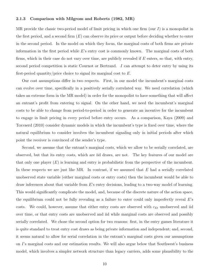
2.1.3 Comparison with Milgrom and Roberts (1982, MR)
MR provide the classic two-period model of limit pricing in which one firm (our I) is a monopolist in
the first period, and a second firm (E) can observe its price or output before deciding whether to enter
in the second period. In the model on which they focus, the marginal costs of both firms are private
information in the first period while E’s entry cost is commonly known. The marginal costs of both
firms, which in their case do not vary over time, are publicly revealed if E enters, so that, with entry,
second period competition is static Cournot or Bertrand. I can attempt to deter entry by using its
first-period quantity/price choice to signal its marginal cost to E.
Our cost assumptions differ in two respects. First, in our model the incumbent’s marginal costs
can evolve over time, specifically in a positively serially correlated way. We need correlation (which
takes an extreme form in the MR model) in order for the monopolist to have something that will affect
an entrant’s profit from entering to signal. On the other hand, we need the incumbent’s marginal
costs to be able to change from period-to-period in order to generate an incentive for the incumbent
to engage in limit pricing in every period before entry occurs. As a comparison, Kaya (2009) and
Toxvaerd (2010) consider dynamic models in which the incumbent’s type is fixed over time, where the
natural equilibrium to consider involves the incumbent signaling only in initial periods after which
point the receiver is convinced of the sender’s type.
Second, we assume that the entrant’s marginal costs, which we allow to be serially correlated, are
observed, but that its entry costs, which are iid draws, are not. The key features of our model are
that only one player (E) is learning and entry is probabilistic from the perspective of the incumbent.
In these respects we are just like MR. In contrast, if we assumed that E had a serially correlated
unobserved state variable (either marginal costs or entry costs) then the incumbent would be able to
draw inferences about that variable from E’s entry decisions, leading to a two-way model of learning.
This would significantly complicate the model, and, because of the discrete nature of the action space,
the equilibrium could not be fully revealing as a failure to enter could only imperfectly reveal E’s
costs. We could, however, assume that either entry costs are observed with cEt unobserved and iid
over time, or that entry costs are unobserved and iid while marginal costs are observed and possibly
serially correlated. We chose the second option for two reasons: first, in the entry games literature it
is quite standard to treat entry cost draws as being private information and independent; and, second,
it seems natural to allow for serial correlation in the entrant’s marginal costs given our assumptions
on I’s marginal costs and our estimation results. We will also argue below that Southwest’s business
model, which involves a simpler network structure than legacy carriers, adds some plausibility to the
10

idea that Southwest’s operating costs might be more transparent than those of other carriers.
2.2 Equilibrium
Unique Nash equilibrium behavior post entry, where two firms play a complete information duopoly
game, is assumed.7 We are therefore interested in characterizing play before E enters. Our basic
equilibrium concept is MPBE (Roddie (2012a), Toxvaerd (2008)). The definition of a MPBE requires,
for each period:
• a time-specific pricing strategy for I, as a function of both firms’ marginal costs ςIt : (cIt, cEt)→
pIt;
• a time-specific entry rule for E, as a function of its beliefs about I’s marginal cost, denoted with
a cIt, its own marginal costs and its own entry cost draw, σEt : (cIt, cEt, κt) → {Enter, Stay
Out}; and
• a specification of E’s beliefs about I’s marginal costs given all possible histories of the game.
In an equilibrium, for all possible cEt and cIt, E’s entry rule should be optimal given its beliefs, its
beliefs should be consistent with I’s strategy on the equilibrium path, and the evolution of marginal
costs, and I’s pricing rule must be be optimal given what E will infer from I’s price and how E will
react based on these inferences.
Fully Separating Riley Equilibrium (FSRE). We will consider an equilibrium where I’s price
perfectly reveals its current marginal cost, i.e., there is full separation, and where signaling is achieved
at minimum cost to I subject to the incentive compatibility constraints being satisfied (i.e. the ‘Riley
equilibrium’ (Riley (1979)).
The following proposition contains our main theoretical results
Proposition 1 Consider the following strategies and beliefs:
(i) E’s entry strategy will be to enter if and only if entry costs κt are lower than a threshold
κ∗t (cIt, cEt), where cIt is E’s (point) belief about I’s marginal cost and
κ∗t (cIt, cEt) = β[Et(φEt+1|cIt, cEt)− Et(V Et+1|cIt, cEt)] (2)
7Existence and uniqueness will depend on the particular form of demand assumed, and will hold for the commondemand specifications (e.g., linear, logit, nested logit) with single product firms and linear marginal cost.
11

where Et(V Et+1|cIt, cEt) is E’s expectation, at time t to being a potential entrant in period t + 1 (i.e.,
if it does not enter now) given equilibrium behavior at t + 1 and Et(φEt+1|cIt, cEt) is its expected value
to being a duopolist in period t + 1 (which assumes it has entered prior to t + 1).8 The threshold
κ∗t (cIt, cEt) is strictly decreasing in cEt and strictly increasing in cIt;
(ii) I’s pricing strategy ςIt : (cIt, cEt)→ p∗It will be the solution to a differential equation
∂p∗It∂cIt
=βg(·)∂κ
∗t (cIt,cEt)
∂cIt{Et[V I
t+1|cIt, cEt]− Et[φIt+1|cIt, cEt]}
qM(pIt) + ∂qM (pIt)∂pIt
(pIt − cIt)(3)
and an upper boundary condition p∗It(cI) = pstatic monopoly(cI). Et[V It+1|cIt, cEt] is I’s expected value of
being a monopolist at the start of period t + 1 given current (t period) costs and equilibrium behavior
at t+ 1. Et[φIt+1|cIt, cEt] is its expected value of being a duopolist in period t+ 1;
(iii) E’s on-the-equilibrium path beliefs: observing an output qIt, E believes that I’s marginal cost
is ς−1It (pIt, cEt).
This equilibrium exists and the above form the unique MPBE strategies and equilibrium-path beliefs
consistent with a recursive application of the D1 refinement. For completeness we assume that if E
observes a price which is not in the range of ςIt(cIt, cEt) it believes that the incumbent has marginal
cost cI .
Proof. See Appendix A.
Our proofs use results from the theoretical literature on signaling models. The first result that we
use is from Mailath and von Thadden (forthcoming). They provide conditions on signaling payoffs9 that
lead to a unique separating equilibrium, where the signaler’s strategy is determined by a differential
equation and a boundary condition.10 The key conditions are type monotonicity (a given price
reduction always implies a greater loss in current payoffs for an incumbent with higher marginal
costs), belief monotonicity (the incumbent always benefits when the entrant believes that he has lower
cIt, which reflects the monotonicity of the entrant’s entry rule) and a single crossing condition (implies
8When we define values we have to do so at specific points in the stage game. Both firms values as duopolists aredefined once they know the current period values of both firms’ marginal costs. For the pre-entry game, E’s value isdefined at point 2 in the stage game defined above where E knows its own marginal cost and its entry cost for theperiod. The value for the incumbent is defined after point 1, when it knows its own marginal cost and the marginal costof the entrant.
9The signaling payoff function can be written as ΠIt(cIt, cIt, pIt, cEt) where cIt is E’s point belief about the incum-bent’s marginal cost when taking its period t entry decision. An alternative way of writing the payoff function that isused when ruling out pooling equilibria is ΠIt(cIt, κEt, pIt, cEt) where κEt is the threshold used by the potential entrant.
10We use Theorem 1 of Mailath and von Thadden (forthcoming), which is effectively a re-statement of a result fromMailath (1987).
12

that a lower cost incumbent is always willing to cut price slightly more in order to differentiate itself
from higher cost incumbents). Our contribution is to show that our assumptions on the primitives of
the model (or more precisely, static monopoly and duopoly quantities and payoffs) are sufficient for I’s
signaling payoff function to satisfy these conditions in every period by applying backwards induction.
Our conditions are not necessary so that our equilibrium may exist more generally.
Mailath and von Thadden’s results do not rule out the possible existence of pooling equilibria.
To do so we recursively apply the D1 refinement (Cho and Sobel (1990), Ramey (1996)), which is
a restriction on the possible inferences that E could make when observing off-the-equilibrium-path
actions. Specifically, in a one-shot signaling game, D1 restricts how off-the-equilibrium-path signals
are interpreted by requiring the receiver to place zero posterior weight on a signaler having a type θ1
if there is another type θ2 who would have a strictly greater incentive to deviate from the putative
equilibrium for any set of post-signal beliefs that would give θ1 an incentive to deviate. Theorem 3
of Ramey (1996) shows that as long as a pool does not involve signalers choosing (in our setting) the
lowest possible price, pooling equilibria can be eliminated when the signaling payoff function satisfies
a single crossing condition.
Applying D1 in a setting with repeated signaling is potentially complicated by the possibility that
an off-the-equilibrium path signal in one period could change how the receiver interprets signals in
future periods. Here we follow Roddie (2012a) in applying a recursive version of D1, where we work
backwards through the game, applying the refinement in each period, assuming refined equilibrium
behavior and inferences in future periods.
2.3 Solving the Model
Given values of the parameters, the supports and the form of the differential equation describing the
incumbent’s pricing strategy it is straightforward to compute pricing strategies and entry probabilities.
The solution algorithm is as follows.
Step 1. Specify a grid for cIt and cEt.
Step 2. For each of these points calculate each firm’s single-period profits in the specified full
information duopoly game that follows entry.
Step 3. Consider period T . Calculate the incumbent’s static monopoly profits for each discretized
value of cIt (in this period it does not face the threat of entry and so prices as a static monopolist).
The incumbent’s static monopoly and duopoly profits define V IT and φIT for each value on the grid.
For the potential entrant V ET = 0 and φET is the static duopoly profit.
13

Step 4. Consider period T − 1.
For a given value of cET−1 we use the known transition matrix of costs to calculate the value of
ET−1[φET |cIT−1, cET−1] for each value of cIT−1. As ET−1[V ET |cIT−1, cET−1] = 0, κ∗T−1(cIT−1, cET−1) =
βET−1[φET |cIT−1, cET−1], and we can compute g(·) and∂κ∗T−1(cIT−1,cET−1)
∂cIT−1for each of these values. Next
we solve for the pricing strategy of the incumbent as a function of its marginal cost, by solving the
differential equation starting from the boundary solution that the firm with the highest marginal cost
sets the static monopoly price
∂p∗IT−1
∂cIT−1
=βg(κ∗T−1)
∂κ∗T−1(cIT−1,cET−1)
∂cIt{ET−1[V I
T |cIT−1, cET−1]− ET−1[φIT |cIT−1, cET−1]}
qM(pIT−1) + ∂qM (pIT−1)
∂pIT−1(pIT−1 − cIT−1)
(4)
This is done using ode113 in MATLAB. Given known demand, the denominator can be computed
exactly for any value of cIT−1 considered by the differential equation solver. We store this result, and
then repeat for all other values of cET−1.
Given the entry and pricing strategies we can calculate V iT−1(cIT−1, cET−1) and φiT−1(cIT−1, cET−1)
for both firms (i.e., the values of each firm as a monopolist/potential entrant/duopolist) as appropriate
given the cost state.
Step 5. Consider period T − 2. Here we proceed using the same steps as in Step 4, except that
κ∗T−2(cIT−2, cET−2) = β{ET−2[φET−1|cIT−2, cET−2]− ET−2[V ET−1|cIT−2, cET−2]}.
Step 6. Repeat for all previous periods.
3 Can Our Limit Pricing Model Explain the “Southwest Ef-
fect”?
We now turn to the question of whether our dynamic limit pricing model can explain why incumbent
carriers cut prices substantially when Southwest becomes a potential entrant on an airline route. We
present two types of evidence. First, in Section 4, we show reduced form evidence that indicates, for
the routes that match the assumptions of our model, that incumbents cut prices because they want
to try to deter entry, and that it is price, rather than route capacity, that is their strategic variable
of choice. Second, in Section 5, we perform a calibration exercise that shows that our model can
generate price cuts consistent with the price changes observed in the data, where we use demand and
cost parameters estimated using airline data. In this section we introduce our data and explain why
we believe that it is plausible that our model may capture important features of at least a subset of
14

airline markets.
3.1 Relevance of Our Model to the Southwest Effect
Competition in airline markets, which we define as routes between airport-pairs11, is heterogenous with
routes between small cities often having no non-stop service, while large markets may have several
carriers competing non-stop. While previous analysis of the Southwest effect (e.g., in GS) has drawn
on this wide range of markets, we will test our model, which assumes an incumbent monopolist, by
focusing on a subset of markets with one dominant incumbent when Southwest is a potential entrant
(defined as Southwest serving both of the endpoint airports but not the route itself) and we will focus
on this carrier’s pricing and how Southwest responds to it. In our markets there are usually several
potential entrants in addition to Southwest but we believe that it is plausible to focus on Southwest
because its rapid growth during our data (1993-2010) and the large effect that it has on prices when
it actually enters make it plausible that incumbents would be particularly concerned to try to prevent
Southwest’s entry.12
The most obvious reason to believe that our model cannot describe what happens in the airline
industry is that we are making very strong assumptions about the observability of costs. Specifically,
we have assumed that, prior to entry, the incumbent’s marginal cost is private information, while
the potential entrant’s marginal costs are public information but its entry costs are unobserved. We
note that, while it would complicate solving our model by adding additional state variables, we could
allow for additional factors, such as fuel costs or changes in the economy, that affect marginal costs
or demand and are observed by both firms, so what is really critical is that there is an idiosyncratic
portion of the incumbent’s costs that are private information and serially correlated.
Why is it reasonable to believe that some part of the incumbent’s marginal cost is not publicly
observed? The dominant incumbents in our sample are almost all legacy carriers operating hub-
and-spoke networks where one of the endpoint airports is a hub. As has been well-documented in
cases of alleged predation (Edlin and Farrell (2004), Elzinga and Mills (2005)), the effective marginal
opportunity cost of a seat on a particular segment on this type of route depends on how people who
might travel on the segment as part of a longer route fly over the rest of the carrier’s network and
the profitability of these onward journeys. These opportunity cost can be difficult to determine
unambiguously even ex-post and with access to the carrier’s internal cost data. Therefore, the
11We follow GS in defining markets as airport-pairs. An alternative approach is to use city-pairs.12Wu (2012) compares the effects that potential entry by Southwest and JetBlue have on incumbent prices. He finds
that JetBlue has a substantially smaller effect.
15

incumbent’s current marginal cost should be somewhat opaque to other firms making contemporaneous
decisions about entry, and that the unobserved component is likely to be time-varying (as travelers
options to use other routes for connections change) but serially correlated.13 In contrast, Southwest’s
marginal costs, which we assume are observed, are likely to be relatively transparent because it operates
a simpler point-to-point network using a fleet composed entirely of Boeing 737s. In our view, the
two informational assumptions that are actually harder to justify are that Southwest’s current entry
costs are unobserved to the incumbent and that the incumbent’s marginal costs are observed once
the potential entrant enters. The first assumption is designed to capture the idea that, even if an
incumbent knows factors that might affect entry, such as the availability of gates, it is likely difficult
for it to determine exactly when Southwest will enter routes that appear likely to be marginal in terms
of Southwest’s profitability. In the context of our model one could interpret this type of uncertainty as
uncertainty about Southwest’s entry cost. The second assumption is primarily for convenience in the
sense that we could follow Roddie (2012a) and allow for a duopoly game with asymmetric information
post-entry, although in doing so we would move further away from the the spirit of the MR model. In
general it also seems plausible that operating on a route should give an entrant a clearer view of the
incumbent’s marginal costs than it has a potential entrant.
While we can defend our cost assumptions, there are clearly important features of the industry that
our model abstracts away from. In particular, a carrier’s marginal costs on different routes are likely
to be correlated so that a potential entrant should try to make inferences about costs on a particular
route from pricing on other routes as well. Our model is a model of a single route and cannot capture
this. On a particular route a carrier also sets many prices (first or business class and economy tickets,
and tickets with and without restrictions that may be available on different dates before departure).
Our model ignores this feature, assuming that the incumbent sets a single price. However, we will
provide evidence that, on at least the routes that fit the assumptions of our model, incumbent carriers
cut prices across the entire distribution of fares, which, at least intuitively, seems consistent with the
idea of a carrier trying to signal that its marginal cost of filling a seat is low. This fact will also
provide some evidence against explanation against alternative explanations for why incumbents cut
prices when Southwest becomes a potential entrant.
13One might object that firms can use publicly collected data to understand these network flows. However, theDepartment of Transportation only releases these data with a lag of at least three months, and our theoretical resultshold even if we assume that the incumbent marginal costs are revealed to the entrant after it has made its entry decision.
16

3.2 Data
Most of our data is drawn from the U.S. Department of Transportation’s Origin-Destination Survey
of Airline Passenger Traffic (Databank 1), a quarterly 10% sample of domestic tickets, and its T100
database that reports monthly carrier-segment level information on flights, capacity and the number
of passengers carried on the segment (which may include connecting passengers), that we aggregate
to the quarterly level. Our data covers the period from Q1 1993-Q4 2010 (72 quarters).14
Following GS, we define a market to be a non-directional airport pair with quarters as periods.
We only consider pairs where, on average, at least 50 DB1 passengers are recorded as making return
trips each period, possibly using connecting service, and in everything that follows a one-way trip is
counted as half of a round-trip. We define Southwest as a potential entrant on a route when it serves
at least one other route directly (defined by having at least 65 flights per quarter recorded in T100, or
50 non-stop passengers in DB1) out of both of the endpoint airports, but it does not serve directly the
route itself. We define Southwest as having entered once it has at least 65 flights recorded in T100
and carries 150 non-stop passengers on the route in DB1.
Based on our potential entrant definition there are 1,872 markets where Southwest becomes a
potential entrant after the first quarter of our data and before Q4 2009, a cut-off that we use so we
can see whether Southwest enters the market in the following year, an observed outcome that we will
use to estimate which market characteristics make entry more likely. Southwest enters 339 of these
markets during the period of our data. We will call this the full sample. Most of our analysis will
focus on the subset of these markets where there is one carrier that is a dominant incumbent before
Southwest enters. As we want to identify only carriers that are committed to a market rather than
just serving it briefly, we use the following rules to identify a dominant carrier:
1. to be active in a quarter it must carry at least 150 DB1 non-stop passengers;
2. once it becomes active in a market the carrier must be active in at least 70% of quarters before
Southwest enters, and in 80% of those quarters it must account for 80% of direct traffic on the
market and at least 50% of total traffic.15
14There are some changes in reporting requirements and practices over time. For example, prior to 1998 operatingand ticketing carriers are not distinguished in DB1, making it difficult to analyze codesharing. Prior to 2002 regionalaffiliates, such as American Eagle or Air Wisconsin operating as United Express, were not required to report T100 data,which provides some limits on our ability to look at capacity.
15To apply this definition we have to deal with carrier mergers (for example, Northwest was the dominant carrier onthe Minneapolis to Oklahoma City route before it merged with Delta in 2008, after which Delta is the dominant carrier).In our baseline specifications we treat the dominant carrier before and after a merger as the same carrier.
17
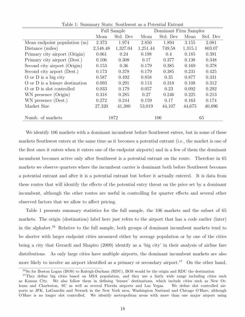
Table 1: Summary Stats: Southwest as a Potential Entrant
Full Sample Dominant Firm SamplesMean Std. Dev Mean Std. Dev Mean Std. Dev
Mean endpoint population (m) 2.373 1.974 2.850 1.894 3.155 2.081Distance (miles) 2,548.48 1,327.04 1,251.44 749,58 1,315.1 803.07Primary city airport (Origin) 0.061 0.24 0.198 0.4 0.185 0.391Primary city airport (Dest.) 0.106 0.308 0.17 0.377 0.138 0.348Second city airport (Origin) 0.153 0.36 0.179 0.385 0.169 0.378Second city arport (Dest.) 0.173 0.378 0.179 0.385 0.231 0.425O or D is a big city 0.587 0.492 0.858 0.35 0.877 0.331O or D is a leisure destination 0.093 0.291 0.113 0.318 0.108 0.312O or D is slot controlled 0.033 0.179 0.057 0.23 0.092 0.292WN presence (Origin) 0.318 0.285 0.27 0.246 0.225 0.213WN presence (Dest.) 0.272 0.244 0.159 0.17 0.163 0.174Market Size 27,320 41,380 53,019 44,107 44,675 40,896
Numb. of markets 1872 106 65
We identify 106 markets with a dominant incumbent before Southwest enters, but in some of these
markets Southwest enters at the same time as it becomes a potential entrant (i.e., the market is one of
the first ones it enters when it enters one of the endpoint airports) and in a few of them the dominant
incumbent becomes active only after Southwest is a potential entrant on the route. Therefore in 65
markets we observe quarters where the incumbent carrier is dominant both before Southwest becomes
a potential entrant and after it is a potential entrant but before it actually entered. It is data from
these routes that will identify the effects of the potential entry threat on the price set by a dominant
incumbent, although the other routes are useful in controlling for quarter effects and several other
observed factors that we allow to affect pricing.
Table 1 presents summary statistics for the full sample, the 106 markets and the subset of 65
markets. The origin (destination) label here just refers to the airport that has a code earlier (later)
in the alphabet.16 Relative to the full sample, both groups of dominant incumbent markets tend to
be shorter with larger endpoint cities measured either by average population or by one of the cities
being a city that Gerardi and Shapiro (2009) identify as a ‘big city’ in their analysis of airline fare
distributions. As only large cities have multiple airports, the dominant incumbent markets are also
more likely to involve an airport identified as a primary or secondary airport.17 On the other hand,
16So for Boston Logan (BOS) to Raleigh-Durham (RDU), BOS would be the origin and RDU the destination17They define big cities based on MSA population, and they use a fairly wide range including cities such
as Kansas City. We also follow them in defining ‘leisure’ destinations, which include cities such as New Or-leans and Charleston, SC as well as several Florida airports and Las Vegas. We define slot controlled air-ports as JFK, LaGuardia and Newark in the New York area, Washington National and Chicago O’Hare, althoughO’Hare is no longer slot controlled. We identify metropolitan areas with more than one major airport using
18

the standard deviations show that both sets of markets are quite heterogeneous with respect to market
characteristics.
The bottom row of the table contains our estimate of market size. We form this estimate as the
predicted value from an OLS gravity model regression where, using data for Q1 1993, we regress the
log of the total number of round-trip passengers on a route on the logs of total enplanements at each
of the endpoint airports and the log of non-stop round trip distance. This prediction is multiplied
by 3.5 to give a rough-and-ready approximation of the total number of people who might travel on a
route if prices were low enough.18
Table 2 reports summary statistics for variables that vary over time for the dominant firm markets,
such as average prices and market shares. Quarters are aggregated into three groups: Phase 1 - before
Southwest is a potential entrant, Phase 2 - after Southwest is potential entrant but before it enters
and Phase 3 - after Southwest enters. The latter set of markets is a selected sample of markets, which
explains why, in Phase 3, the number of seats that the incumbent has scheduled and the number
of passengers it carries on these routes is significantly larger than for the broader set of markets in
Phases 1 and 2. In these summary statistics we observe that the incumbent’s prices tend to be lower
in Phase 2 than Phase 1, consistent with the Southwest Effect. If Southwest enters, incumbents tend
to charge prices that are slightly above Southwest but still tend to maintain a larger market share.
This is consistent with incumbents being viewed by consumers as having higher quality.
The summary statistics also provide some evidence against an alternative story for why prices fall
in Phase 2. Recall that in Phase 2, Southwest serves both endpoint airports so that it is plausible that
a passenger might choose to travel using connecting service on Southwest, so that Southwest might
really be a competitor rather than just a potential entrant. However, from the table we see that
Southwest’s average market share in Phase 2 is less than 2%, compared with the dominant carrier’s
share of over 80%, suggesting that the degree of direct competitive pressure that Southwest exerts in
Phase 2 is fairly small. This contrasts with the much larger share that Southwest typically attains if
it enters the market.
The bottom section of the table shows the number of carriers providing indirect service (to count a
carrier must carry at least 6.5 DB1 return passengers), the total number of potential entrants (carriers
serving both endpoints) and a measure of the importance of code-sharing on the route, measured
http://en.wikipedia.org/wiki/List of cities with more than one airport, and identify the primary airport in a city asthe one with the most passenger traffic in 2012.
18The advantage of this approach is that it adjusts for distance (as more people travel between closer cities) and, formulti-airport cities, endpoint enplanements allow us to get a better prediction of the number of people traveling thatjust using endpoint city populations.
19

either by at least one of the passengers in DB1 being identified as a codesharing passenger (operating
carrier is the dominant incumbent but the ticketing carrier is different) or the number of codeshared
passengers. Goetz and Shapiro (2012) argue that one of the responses to the threat of entry by
Southwest is that incumbents increase codesharing. For our dominant firm sample, we also see the
proportion of code-shared routes increasing in Phase 2. However, we will show below that this occurs
primarily in markets where Southwest’s actual entry is most likely, which is different from the set of
routes where we observe the largest price decreases.
4 Evidence of Limit Pricing in the Dominant Incumbent
Sample
We begin our analysis by confirming that we do find a statistically significant Southwest Effect, i.e.,
that prices fall in Phase 2 when Southwest becomes a potential entrant, for our dominant incumbent
sample once we control for market fixed effects, quarter dummies and other controls. To do so, we
follow GS, who used markets with any number of incumbents, by utilizing the following regression
specification:
ln(pj,m,t) = γm + τt + αXj,m,t
+8+∑
τ=−8
βτSWPEm,t0+τ +3+∑τ=0
βτSWEm,te+τ + εj,m,t (5)
where pj,m,t is the passenger-weighted mean fare charged by dominant incumbent carrier j in market
m in quarter t, γm are market-carrier fixed effects19 and τt are quarter fixed effects. Carriers other
than the dominant carrier are not included in our version of the regression. X includes the number
of firms serving the market (with direct or connecting service) as well as interactions between the jet
fuel price and route distance. t0 is the quarter in which Southwest becomes a potential entrant, so
SWPEm,t0+τ is an indicator for Southwest being a potential entrant into market m at quarter t0 + τ .
If Southwest enters it does so at te, and SWEm,te+τ is an indicator for Southwest being direct entrant
into the market at quarter te+τ . We use observations for up to 3 years (12 quarters) before Southwest
becomes a potential entrant, and the β coefficients measure price changes relative to those quarters
19Note that when the dominant firm is involved in a merger (for example, the merger between Delta and Northwestin 2008) we use the same fixed effect before and after the merger even though the name of the dominant carrier maychange (e.g., from Northwest to Delta on the Minneapolis to Omaha route).
20

Tab
le2:
Sum
mar
ySta
ts:
Dom
inan
tC
arri
erSam
ple
Phas
e1:t<t 0
Phas
e2:t 0≤t<t e
Phas
e3:t≥t e
Var
iable
Mea
nStd
.D
evM
ean
Std
.D
evM
ean
Std
.D
ev
Incu
mbe
nt
Pri
cin
gM
ean
fare
511.
9216
2.89
447.
6512
0.33
259.
8873
.24
Sou
thw
est
Pri
cin
gM
ean
fare
-37
1.95
78.0
122
3.34
64.1
9
Incu
mbe
nt
Tra
ffic
T10
0Sea
tssc
hed
ule
d76
,798
55,0
8776
,570
44,9
6911
5,40
563
,096
T10
0Seg
men
tpas
senge
rs49
,092
34,1
6556
,694
35,7
0182
,277
45,0
59
Incu
mbe
nt
Mar
ket
Sha
reT
otal
shar
e0.
740.
264
0.83
0.15
0.51
70.
228
Sou
thw
est
Mar
ket
Sha
reT
otal
shar
e-
0.01
370.
0332
0.43
40.
232
Rou
teC
hara
cter
isti
csC
omp
etit
ors
indir
ect
1.87
1.58
1.85
1.33
0.97
1.25
Pot
enti
alen
tran
ts7.
831.
718.
251.
628.
551.
88In
cum
ben
tco
de-
shar
edro
ute
0.15
10.
357
0.35
40.
478
0.47
00.
499
Incu
mb
ent
code-
shar
edpas
senge
rs(D
B1B
)4
29.2
94.
5413
.42
20.8
979
.76
Num
ber
mar
kets
106
6554
21

that are more than 8 quarters before Southwest becomes a potential entrant or, if Southwest becomes
a potential entrant within the first 8 quarters that the dominant carrier is observed in the data, the
first quarter that it is observed. We estimate separate coefficients for the quarters immediately around
the entry events, but aggregate those quarters further away from the event where we have fewer
observations. Standard errors are clustered at the market-carrier level to allow for correlation in the
error terms over time. We report results where markets are weighted equally, but the results are very
similar if, like GS, we weight markets by the average number of passengers carried.
Table 4 presents the coefficient estimates. Consistent with GS’s results using a broader sample
and the summary statistics discussed above, Southwest’s presence as a potential entrant, as well as its
actual entry, is associated with large falls in the dominant incumbent’s price. Southwest’s presence as a
potential entrant leads to price declines of around 10-14% in the six quarters after Southwest becomes
a potential entrant. These price declines are maintained over time, i.e., they do not disappear if
Southwest fails to enter the route. This is consistent with our model where, because the incumbent’s
marginal cost can change over time, there is an incentive to continue signal. In fact the decline seems
to increase over time: this is also consistent with our model because of the way that those incumbents
who repeatedly deter entry will tend to be those who receive the most favorable cost draws so that
both their profit-maximizing and their deterring prices will tend to be lower. Like GS, prices start to
fall about two quarters before Southwest becomes a potential entrant, presumably reflecting the fact
that Southwest’s airport entry is either announced or otherwise anticipated several months before it
actually begins flying routes. If Southwest enters the market, average prices decline by an additional
30-45%, giving a decline of 45-60% relative to prices in Phase 1. This post-entry decline is larger
than the one in GS, presumably reflecting the fact that dominant incumbents have more market power
prior to Southwest’s entry than the average incumbent in GS’s sample.
We now address the question of whether our model of entry deterrence through limit pricing can
explain the price declines that occur when Southwest becomes a potential entrant. We begin by using
the approach to detecting strategic investment suggested by EE to identify whether the price declines
are likely due to the dominant incumbents trying to deter entry. In the context of a fairly general
incomplete information model of strategic investment EE argue that, when strategic incentives are
present, they lead to a prediction that the relationship across markets between the level of investment
and factors that affect the attractiveness of entry and investment should be non-monotonic. In the
context of our model, the logic would apply in the following way. Suppose that we can identify how
attractive markets are to Southwest based on exogenous market characteristics. When Southwest
22

Table 3: Incumbent Responses to the Threat of Entry - Logged Average Fare
β Estimates
Before WN is PE: WN is PE: WN is E:t0 − 8 -0.047 t0 −0.105∗∗∗ te −0.416∗∗∗
(0.029) (0.031) (0.066)
t0 − 7 -0.022 t0 + 1 −0.115∗∗∗ te + 1 −0.514∗∗∗
(0.0307) (0.034) (0.069)
t0 − 6 -0.040 t0 + 2 −0.131∗∗∗ te + 2 −0.539∗∗∗
(0.034) (0.032) (0.077)
t0 − 5 -0.041 t0 + 3 −0.131∗∗∗ te + 3 −0.602∗∗∗
(0.034) (0.032) (0.080)
t0 − 4 -0.015 t0 + 4 −0.135∗∗∗ te + 4 −0.608∗∗∗
(0.033) (0.034) (0.082)
t0 − 3 −0.009 t0 + 5 −0.137∗∗∗ te + 5 −0.577∗∗∗
(0.029) (0.038) (0.084)
t0 − 2 −0.0761∗∗ t0 + 6-12 −0.206∗∗∗ te + 6-12 −0.589∗∗∗
(0.029) (0.047) (0.081)
t0 − 1 −0.0874∗∗∗ t0 + 13+ −0.309∗∗∗ te + 13+ −0.589∗∗∗
(0.029) (0.051) (0.086)
Market-Carrier Fixed Effects: YesQuarter Fixed Effects: YesTime-varying Controls: Yes
N 3,904adj. R2 0.81
Dependent variable is log of the mean passenger-weighted fare. Standard errors are inparentheses and are clustered by route-carrier. ∗∗∗ denotes significance at the 1% level,∗∗ at 5% and ∗ at 10%.
becomes a potential entrant, an incumbent will not choose to cut prices (very much) in markets where
entry is very unattractive to Southwest, because it is likely only to be sacrificing monopoly profits. A
low price is also unlikely to deter entry in markets where entry is very attractive, so the monopolist will,
once again, not want to sacrifice short-run profits that it can make before Southwest enters. Instead,
the incumbent will only be willing to cut prices substantially in markets of intermediate attractiveness
to Southwest, where its entry decision might plausibly be tipped away from entry, towards delay, if it
believes that the incumbent has low marginal costs. On the other hand, if, instead of being motivated
by deterrence, incumbents cut prices to accommodate entry, i.e., to generate outcomes that are more
favorable for the incumbent once entry occurs, then we would expect to see the size of the price declines
to increase monotonically with how attractive markets are to the entry of Southwest.20
20GS consider a simpler version of this analysis where they compare pricing behavior, in the quarters immediatelyprior to Southwest becoming a potential entrant on routes where Southwest had already announced it would enter and
23

The EE approach is implemented in two stages (second stage standard errors are corrected for first
stage estimation error using a bootstrap where we resample markets). In the first stage, we estimate
a probit model using the full sample, where an observation in a market and the dependent variable is
equal to 1 if Southwest entered within four quarters of becoming a potential entrant.21
Pr(entry4m = 1|X,Z, t) = Φ(τt + αXm) (6)
t is the quarter that WN became a PE, and τt are time dummies. The Xm variables are exogenous
market characteristics such as measures of market population, route distance and whether one of
the endpoints is a big city, a tourist destination or a primary/secondary airport in a large city, and
measures of both the dominant incumbent’s presence and Southwest’s presence. We also include our
measure of market size (divided by 10 in this case). The estimates are in Table 4, and the signs on
most of the coefficients are sensible so that, for example, there is more entry in both larger and shorter
markets. The fit of the model is also good for an entry model, with a pseudo-R2 of 0.37.
In the second stage, we take the dominant firm sample and use the first-stage estimates and the
exogenous characteristics of these markets to predict the probability of entry. We then divide these
markets into terciles based on the probability of entry, and estimate the following regression:
ln(pj,m,t) = γm + τt + αXm,t +3∑s=1
βsI[ρm ∈ Tercs] ∗ SWPEm,t + εj,m,t (7)
where ρm is the predicted probability of entry (within one year) on market m and, as before, pj,m,t is
the passenger-weighted mean fare charged by the dominant incumbent carrier j in market m in quarter
t. Xm,t is defined as the same as before. All of the specifications we consider include market-carrier
and quarter fixed effects. We focus on the results where we use fuel interacted with distance and
deviation from mean distance squared to control for how jet fuel prices and distance affect carriers
costs, but the results are robust to using different controls. Only observations from Phases 1 and 2
are included in the regression, and the βs coefficients measure how much prices decline in Phase 2 as
a function of the probability of entry. The results are similar if we use quintiles rather than terciles,
although the individual coefficients tend to be less significant because of the smaller number of markets
routes where it had not. They observe larger declines in prices on routes where entry had not been pre-announced, butthe differences are generally not statistically significant. However, the direction of their results is consistent with ourfindings.
21It would be inappropriate to use a dummy for Southwest ever entering because, in our relatively long sample,different markets are exposed to the possibility of entry for different periods of time. Using a 4 quarter rule also meansthat we minimize the truncation problem associated with the end of the sample while still having a significant numberof observations.
24

Table 4: First Stage
(1)entry4
Secondary airportO 0.542**(0.237)
Secondary airportD 0.0383(0.233)
Primary airportO 0.688***(0.254)
Primary airportD 0.558***(0.211)
WNpresORG 2.455**(0.983)
WNpresORG2 -2.245**(0.940)
WNpresDEST 0.187(1.045)
WNpresDEST 2 -0.0427(1.101)
INCpresORG 2.174(1.743)
INCpresORG2 -2.085(1.683)
INCpresDEST -4.076(4.223)
INCpresDEST 2 6.253(7.521)
Slot controlled -1.801***(0.543)
Tourist 1.003***(0.174)
Big city -0.0134(0.146)
Distance -0.668***(0.204)
Distance2 0.0385(0.0344)
Population -0.0952(0.109)
Population2 0.0117*(0.00637)
MarketSize 0.237***(0.0404)
MarketSize2 -0.00745***(0.00165)
N 1872pseudo R2 0.372
Standard errors in parentheses
Additional controls included (e.g. quarter dummies for when Southwest becomes a potential entrant)
* p < 0.10, ** p < 0.05, *** p < 0.01 25

in each group.
The results in the first column of Table 5 indicate that the price declines are only significantly
different from zero, and are largest, in the middle tercile. In contrast, declines are small, at most,
in markets where entry is either likely or unlikely. This pattern is consistent with a limit pricing
deterrence story, but not an accommodation story.
Table 5: Ellison and Ellison Analysis: Second Stage
(1) (2) (3) (4) (5) (6)log(Fare) log(T100 pass.) log(Load) Codeshare route Prop. Codeshare log(Capacity)
Tercile1 -0.0426 0.132* 0.0779** -0.00953 0.00368 0.0799(0.0589) (0.069) (0.033) (0.0986) (0.0047) (0.0756)
Tercile2 -0.142** 0.209** 0.164*** 0.165 0.0114 0.0390(0.0677) (0.0933) (0.037) (0.174) (0.0128) (0.1097)
Tercile3 -0.0692 0.00960 -0.00953 0.444*** 0.0551*** 0.0329(0.091) (0.009) (0.0466) (0.148) (0.0186) (0.0997)
N 3622 3100 3100 2185 2185 3085R2 0.729 0.817 0.690 0.505 0.326 0.730
Bootstrapped standard errors in parentheses
* p < 0.10, ** p < 0.05, *** p < 0.01
One can also take other approaches to examining the empirical plausibility of explanations based
on entry accommodation. For example, the accommodation story that has been mentioned to us
most frequently is that incumbents may cut prices in order to build up the loyalty of their frequent
flyers in order to retain as much of their custom as possible if and when Southwest enters.22 If so,
it seems plausible that we would see price reductions targeted at the types of high-priced tickets that
are usually purchased by frequent flyers when traveling for business. In the Appendix Tables B.1-B.3,
we report the GS results using the logs of the 25th, 50th and 75th percentiles of the fare distribution as
dependent variables rather than the log of the mean fare. Comparing prices in phases 1 and 2, we see
significant and substantial declines across the price distribution, although the proportional declines
are admittedly larger for higher priced tickets. While this seems inconsistent with an accommodation
story based on the dynamics of frequent-flyer demand it does seem intuitively consistent with a limit
pricing deterrence story where the incumbent is trying to signal that its marginal cost of a seat is low,
whichever type of customer purchases it.23
22Specifically an accommodation story requires that there is a state variable that the incumbent can affect by itspricing behavior prior to Southwest’s entry that will affect its demand or costs after Southwest enters. Frequent flyermileage provides this type of state variable.
23The percentile results also provide some additional evidence against the argument that prices fall because Southwest
26

An alternative explanation for why prices decline is that the presence of Southwest at both end-
points is correlated with an actual reduction in the incumbent carrier’s marginal costs on the route,
because it affects how traffic flows over the incumbent’s network (e.g., it affects how many people
fly the route as a segment on a longer journey). While it is not obvious why this would primarily
affect routes with intermediate entry probabilities (e.g., the middle tercile), we can also assess this
explanation directly by repeating the tercile specification using the log of total passenger traffic for
the dominant incumbent on the segment, as measured in T100, as the dependent variable.24 The
results are reported in the second column of Table 5. We observe that once Southwest becomes a
potential entrant segment traffic tends to increase, on average, across all of the terciles although the
increases are not significant on markets where entry is most likely. The finding that traffic increases,
and that there is not a dramatic difference between markets with intermediate entry probabilities and
those with low entry probabilities, provides evidence against the argument that prices fall because of
marginal cost changes.
In the third column of Table 5 we also use the log of the incumbent carrier’s load factor on a route
as the dependent variable. The load factor is measured as the number of passengers carried on the
segment divided by the number of seats scheduled (there are a handful of observations where no seats
were scheduled but some were performed, which explains why the number of observations in column
(3) is slightly less than the number of observations in column (2)). In the sixth column the log of the
number of scheduled seats is used as the dependent variable. Even if segment traffic increases, the
carrier’s marginal cost could fall if it adds so much capacity that there are more empty seats. In
particular, one might argue that this is exactly what would happen if incumbent carriers use capacity
as their strategic variable, as assumed in the models of predatory pricing by airlines proposed by
Snider (2009) and Williams (2012).25 In this case falling prices would be a consequence of an entry
deterring strategy, that might well be focused on markets with intermediate entry probabilities, rather
than the deterring strategy itself. However, we observe that load factors actually tend to increase
once Southwest becomes a potential entrant in markets with intermediate entry probabilities, while
is providing actual competition because it is able to offer connecting service on the route. If so, one would probablyexpect to see the declines concentrated in the lower part of the fare distribution as the types of price-sensitive consumerwho are most likely to be willing to use connecting service on Southwest are also likely to be buy the cheapest, mostrestrictive tickets on the incumbent carrier. Instead we observe similar declines across the price distribution.
24We have fewer observations in this regression because of incomplete coverage of flights operated by regional affiliatesin T100 prior to 2001.
25For example, suppose that the incumbent’s marginal cost is publicly observed and a decreasing function of itscapacity on a route, that it is costly for the incumbent to adjust its route capacity and that Southwest’s post-entryprofits are decreasing in the incumbent’s route capacity. In this case, the incumbent may invest in more capacity to tryto deter in the intermediate entry probability markets, and the incumbent’s price would tend to fall as a result evenwhen it just sets a static profit-maximizing price given the capacity that it has.
27

capacities do not change. This suggests both that marginal costs should not be falling differentially on
these routes and that, if incumbents are trying to deter entry, it is price rather than capacity that is
used as the strategic variable. This result is also consistent with GS’s finding that incumbent capacity
does not systematically increase when Southwest becomes a potential entrant.
Goetz and Shapiro (2012) suggest that incumbents also respond to the threat of entry by Southwest
by increasing codesharing with other carriers, although it is not clear whether this is a strategy that
they use to try to deter or to accommodate entry. To understand whether codesharing is a strategy that
changes in a similar way to pricing we repeat the tercile regressions using two measures of codesharing
as the dependent variable. The first dependent variable is a dummy variable that is equal to 1 if
any DB1 passengers are recorded as flying on the incumbent carrier (as an operating carrier) but with
a different airline as the ticketing carrier during the quarter. This is the Goetz and Shapiro (2012)
measure of codesharing. The second dependent variable is the proportion of passengers carried by
the incumbent that have a different ticketing carrier, which may do a better job of capturing how
important codesharing actually is. We restrict our analysis to quarters after 1998 when operating
and ticketing carriers are distinguished in DB1. The results, reported in the fourth and fifth columns
of Table 5, are interesting because they indicate that, once Southwest becomes a potential entrant,
codesharing increases substantially only in markets where Southwest’s actual entry is most likely. This
suggests that, unlike price reductions, codesharing is likely used as part of an entry accommodation
strategy.
5 Can Our Model Predict the Size of the Observed Price
Declines?
While the reduced-form evidence is consistent with prices being lowered in an attempt to deter entry
(limit pricing), this does not mean that our model can explain the quite large price declines that are
observed. In this section we therefore calibrate our model using estimated demand and cost parameters
to test whether a limit pricing explanation can generate price declines as large as those that are actually
observed. We stay as close as we can to the theoretical model presented above, and our model has the
following features:
• a nested logit demand structure where the nests are ‘fly’ and ‘not fly’ , and the product quality
of the incumbent and Southwest are held constant. The nesting parameter, price coefficient and
28

product qualities are estimated from the data, given the definition of market size from Section
3.
• marginal costs of both firms that evolve according to independent AR(1) processes (with trun-
cated normal innovations) on supports that are different for Southwest and the incumbent,
although we use the same AR(1) parameter for both firms. We estimate the serial correlation
parameter, and choose the supports based on the distribution of marginal costs that we estimate.
• a truncated normal entry cost distribution for Southwest which we choose (i.e., we do not,
currently, recover this from estimating a dynamic entry model). We briefly discuss the plausibility
of the assumed values below.
To estimate demand and marginal costs we use the dominant firm sample data for Phases 1 and 3
(i.e., before Southwest becomes a potential entrant, and after Southwest enters, if it enters). We do this
principally because we want to recover marginal costs using periods when the standard Bertrand Nash
first order conditions may apply, without using periods when the more complicated, dynamic limit
pricing first order conditions might be appropriate. We also restrict attention to only the dominant
incumbent and Southwest (Phase 3), including more marginal carriers who may fly some passengers
on the route in the outside good.
Demand Estimation
We assume a standard nested logit indirect utility specification (e.g., Berry (1994))
ui,j,m,t = µj + τ1Tt + τ2Q2t + τ3Q3t + τ4Q4t + γXj,m,t + αpj,m,t + ξj,m,t + ζFLYi,m,t + (1− λ)εi,j,m,t
≡ θj,m,t + αpj,m,t + ξj,m,t + ζFLYi,m,t + (1− λ)εi,j,m,t (8)
where µj is firm j’s mean quality, Tt is a time trend, and Q2, Q3 and Q4 are seasonal dummies. pj,m,t
is the passenger weighted average round trip fare for firm j on market m in quarter t and ξj,m,t is
the unobserved (to the econometrician) characteristic. In this specification ξj,m,t varies across time
for the same carrier in a given market, but when we do the calibration we will hold the qualities of
the incumbent and Southwest fixed at their estimated mean values. Xj,m,t includes an indicator for
whether the market is a hub for carrier j, together with market characteristics such as distance and
whether one of the airports is a primary or secondary airport. However, because market size is defined
using a regression model which already includes factors such as airport enplanements and distance, we
29

do not necessarily expect these characteristics to have significant effects on demand, and in practice
their effects are statistically insignificant or small. Being a hub carrier may raise demand because of
frequent flyer programs or gate access.
We estimate the model using the standard estimating equation for a nested logit model with
aggregate data (Berry (1994)):
ln
(sj,m,ts0,m,t
)= µj + τ1Tt + τ2Q2t + τ3Q3t + τ4Q4t + γXj,m,t − αpj,m,t + λln(sj,m,t|FLY ) + ξj,m,t (9)
where sj,m,t|FLY is firm j’s market share conditional on flying and sj,m,t is firm j’s market share, and
market size is defined as in Section 3.
As both pj,m,t and sj,m,t|FLY should be endogenous, we instrument for them in our preferred speci-
fication using the one-period lagged value price of jet fuel26 both on its own and interacted with route
distance, each carrier’s competitor’s average presence at the endpoints in that quarter and for the
incumbent whether Southwest has entered the market and for Southwest whether the route involves a
hub for the incumbent.
Table 6 presents estimates of demand when we use OLS and 2SLS. As expected, estimated demand
is more elastic controlling for endogeneity, and the median elasticity in the second column is 3.13,
which is comparable to estimates in other studies of airline demand (e.g., Berry and Jia (2010),
Snider (2009)). Southwest’s quality is estimated to be slightly lower than most of the legacy carriers,
consistent with the fact that post-entry they typically have similar market shares while Southwest has
lower prices. Consistent with Borenstein (1989) and Berry (1992), consumers are estimated to prefer
a carrier that has a hub at one of the endpoints.
When we simulate the calibrated model of dynamic limit pricing below, we will set λ = 0.878 and
the values of θ for each firm by setting Southwest’s quality to be its estimated value (θWN = −0.216),
and the incumbent to have quality equal to the average of the legacy carriers (θINC = 0.196).27
Marginal Costs
With the 2SLS demand estimates in hand, we back out the incumbent’s and Southwest’s marginal
costs in each period using the standard static Bertrand Nash pricing first-order conditions (recall,
Phase 2, where we believe our limit pricing model may apply is not used for estimation). The median
26Specifically, U.S. Gulf Coast Kerosene-Type Jet Fuel Spot Price FOB (in $/gallon).27Distance is set equal to its mean, while the hub, primary and secondary airport parameters are set equal to zero.
30

Table 6: Nested Logit Demand Estimates
OLS 2SLS
α -0.124∗∗∗ -0.346∗∗∗
(0.012) (0.033)
λ 0.722∗∗∗ 0.878∗∗∗
(0.021) (0.044)
µ:AA -0.061 -0.024
(0.047) (0.058)
AS -0.023 -0.108∗∗
(0.045) (0.049)
CO 0.047 0.344∗∗∗
(0.09) (0.113)
DL -0.171∗∗∗ -0.223∗∗∗
(0.043) (0.044)
NW -0.075 0.412∗∗∗
(0.056) (0.102)
UA -0.502∗∗∗ -0.372∗∗∗
(0.071) (0.080)
US 0.015 0.264∗∗∗
(0.044) (0.068)
WN -0.029 -0.194∗∗∗
(0.042) (0.043)
γ:HUB 0.312∗∗∗ 0.396∗∗∗
(0.021) (0.025)
N 6,893 6,893
Market characteristics (e.g., distance,distance2), a linear time trend and quarter-of-year dummies are also included. In thesecond specification we include one-period-lagged value of the average cost of jet fuel,the lagged cost of jet fuel interacted withdistance, each carrier’s competitor’s averagepresence at the endpoints in that quarterand for the incumbent whether Southwesthas entered the market and for Southwestwhether the route involves a hub for theincumbent as instruments for pj,m,t andsj,m,t|FLY . Standard errors are in parenthe-ses. ∗∗∗ denotes significance at the 1% level,∗∗ at 5% and ∗ at 10%.
31

implied marginal cost is $0.16/mile, which is comparable to the $0.14 of total operating expenses per
available seat mile that airlines reported on DOT form 41 in 2010. To estimate the persistence in
marginal costs we then regress the implied costs on lagged costs, market-carrier fixed effects, quarter-
of-year dummies, a time trend, the jet fuel price and the jet fuel price interacted with distance.28 The
estimated AR(1) parameter is shown in the first column of Table 7. As the implied marginal costs are
likely to be measured with error (partly because market shares and prices are based on a sample of
DB1 data), in the second column we instrument for the lagged marginal cost with the previous (i.e.,
t − 2) marginal cost and the value of ρ increases to 0.818, indicating that marginal cost shocks are
quite persistent. The estimated standard deviation of the marginal cost innovations is $25.
Table 7: Marginal Cost Evolution Estimates
OLS 2SLS
mcj,m,t−1 0.747∗∗∗ 0.818∗∗∗
(0.021) (0.013)
N 6,623 6,379
The dependent variable is mcj,m,t, carrier j’s computed marginal cost inmarket m in quarter t. The specification also includes one period laggedfuel price, included separately and also interacted with distance, three quar-ter dummies and a quarterly trend. We also include carrier market fixedeffects. In the second column we instrument for mcj,m,t−1 with mcj,m,t−2.Standard errors are in parentheses. ∗∗∗ denotes significance at the 1% level,∗∗ at 5% and ∗ at 10%.
We set the bounds on marginal costs by choosing values which are approximately at the 25th and
75th percentiles of the estimated marginal costs. For incumbents this gives bounds of [$150,$400], and
for Southwest bounds of [$90,$200], which reflects the fact that Southwest’s observed prices are lower
across markets. We specify the unconditional mean for each firm’s marginal cost to be the center point
of these intervals.
Entry Costs
We use these estimated demand and cost parameters to calibrate our model of dynamic limit pricing
to predict an incumbent’s pricing behavior in a medium-sized market when it faces a new potential
entry threat by Southwest. We consider a case where the market size is equal to its mean value for
the dominant firm markets and set T = 20 and the quarterly discount factor β to 0.98.29. In our
28When we perform the calibration we do not include the effects of time varying fuel costs or time effects in the model.29Given our assumptions on entry costs the incumbent’s equilibrium pricing strategy is quite stable across the early
periods for T = 20.
32

calibration, we set κ ∼ TRN($15m, $9m, $0, $100m).30 To put the mean entry costs in perspective, we
estimate that the average quarterly variable profit for the observations in the dominant firm sample
data in Phases 1 and 3 (based on imputed marginal costs) is $1.66m (Berry and Jia (2010) estimate
this number for all flights and fare classes to be $1.45m in 2006), a figure that implies that for a firm
considering entering in the first period, that an entry cost of $15m represents about 54% of the present
discounted value of future variable profits.
Calibration Results
Figure 1 illustrates the magnitude of price cuts that our calibrated model of limit pricing predicts
relative to the static monopoly pricing schedule in the first period of the game when Southwest’s
marginal cost is at its median ($150). At this point, the most efficient incumbent faces a probability
of entry of 0.2406 in the next period and the least efficient faces a probability of entry of 0.3265. This
level and variance of probability of entry generates shading of 4.7% for an incumbent with marginal
cost equal to $394, (the weakest type, with a marginal cost of $400, sets the Nash price) and maximum
shading by an incumbent of 18.5%; weighted-average shading31 is 15.5%. Recalling that the price cuts
that we observe in the data when Southwest becomes a potential entrant are in the range of 10-15%
, our results suggest that a reasonably parameterized version of the dynamic limit pricing model
generates is capable of generating the type of price changes observed in the data.
Figure 1: Pricing Strategies, t = 1 out of T = 20, cWN = 150.
30Where TRN(µ, σ, a, b) indicates a normal distribution with mean µ, standard deviation σ that is truncated belowat a and above at b.
31Where weights are determined by the probability of each marginal cost combination in the steady state distributionsof costs.
33

As a further test of the model, in the spirit of EE, we can also examine how incumbents’ price
cutting changes in markets that are much smaller or larger than the average (we do this by considering
market sizes at the 10th and 90th percentiles observed in our sample). In these markets we expect to see
much smaller price reductions as deterrence is either largely unnecessary (smaller markets) or unlikely
to be effective (larger ones). Figure 2 confirms these intuitions, as we see weighted average deviations
from static monopoly pricing of 2-3% for each type of market, with corresponding probabilities of entry
of 93-99% and 2-3% for the large and small markets, respectively.
Figure 2: Pricing Strategies, t = 1 out of T = 20, cWN = 150. The right-hand figure is for a largemarket size and the left-hand figure is for the small market size.
6 Conclusion
We have proposed a framework for analyzing a classic form of strategic behavior, entry deterrence by
setting a low price, in a dynamic setting. Under some weak conditions on the primitives and a standard
refinement, our model has a unique Markov Perfect Bayesian Equilibrium in which the incumbent’s
pricing policy reveals his marginal cost each period. This characterization of the equilibrium makes it
straightforward to compute equilibrium policies. The resulting tractability stands in contrast to the
widely-held belief that dynamic games with persistent asymmetric information are too intractable to
be studied or tested empirically, at least when using standard equilibrium concepts. While our model
is a special case in many respects, and uniqueness of a dynamic MPBE is certainly not general, it is the
natural extension of one of the most widely cited static theory models (Milgrom and Roberts (1982)),
and it seems quite plausible that there are other interesting models with structures that would also
make them tractable for dynamic analysis.
We exploit tractability to study whether our model of dynamic limit pricing can explain the so-
called “Southwest effect” where incumbent carriers cut prices when Southwest becomes a potential
34

entrant on a particular airline route. Here we provide new evidence, both in the reduced form and
through a calibration of our structural model, that limit pricing can explain both the qualitative
pattern and the quantitative size of the price cuts. We believe that this type of exercise, which
combines different types of empirical analysis, provides a potentially profitable direction for testing
models of strategic investment.
We hope to extend our analysis in several directions in future work. One priority is to allow for
there to be multiple incumbents and to see whether we can also get tractability in this context, and
under what conditions. This would be an important extension because there are multiple incumbents
in many settings that interest IO economists, including some airline markets where the “Southwest
effect” may be observed.
35

References
Bain, J. (1949): “A Note on Pricing in Monopoly and Oligopoly,” American Economic Review, 39(2),
448–464.
Baron, D. P. (1973): “Limit Pricing, Potential Entry and Barriers to Entry,” American Economic
Review, 63(4), 666–674.
Belleflamme, P., and M. Peitz (2009): Industrial Organization: Markets and Strategies. Cam-
bridge University Press.
Berry, S., and P. Jia (2010): “Tracing the Woes: An Empirical Analysis of the Airline Industry,”
American Economic Journal: Microeconomics, 2(3), 1–43.
Berry, S. T. (1992): “Estimation of a Model of Entry in the Airline Industry,” Econometrica, 60(4),
889–917.
Berry, S. T. (1994): “Estimating Discrete-Choice Models of Product Differentiation,” RAND Jour-
nal of Economics, 25(2), 242–262.
Borenstein, S. (1989): “Hubs and High Fares: Dominance and Market Power in the U.S. Airline
Industry,” RAND Journal of Economics, 20(3), 344–365.
Chevalier, J. (1995): “Capital Structure and Product Market Competition: Empirical Evidence
from the Supermarket Industry,” American Economic Review, 85(3), 415–435.
Chicu, M. (2012): “Dynamic Investment and Deterrence in the U.S. Cement Industry,” Northwestern
University Working Paper.
Cho, I., and J. Sobel (1990): “Strategic Stability and Uniqueness in Signaling Games,” Journal of
Economic Theory, 50(2), 381–413.
Clark, J. M. (1940): “Toward a Concept of Workable Competition,” American Economic Review,
30(2), 241–256.
Dafny, L. (2005): “Games Hospitals Play: Entry Deterrence in Hospital Procedure Markets,” Journal
of Economics & Management Strategy, 14(3), 513–542.
De Bondt, R. (1976): “Limit Pricing, Uncertain Entry and the Entry Lag,” Econometrica, 44(5),
939–946.
36

Edlin, A., and J. Farrell (2004): Antitrust Revolution: Economics, Competition and Policy chap.
The American Airlines Case: A Chance to Clarify Predation Policy. Oxford University Press.
Ellison, G., and S. Ellison (2011): “Strategic Entry Deterrence and the Behavior of Pharmaceu-
tical Incumbents Prior to Patent Expiration,” American Economic Journal: Microeconomics, 3(1),
1–36.
Elzinga, K., and D. Mills (2005): The Antitrust Revolution chap. Predatory Pricing in the Airline
Industry: Spirit Airlines v. Northwest Airlines. Oxford University Press.
Ericson, R., and A. Pakes (1995): “Markov-Perfect Industry Dynamics: A Framework for Empir-
ical Work,” Review of Economic Studies, 62(1), 53–82.
Fershtman, C., and A. Pakes (2012): “Dynamic Games with Asymmetric Information: A Frame-
work for Empirical Work,” Quarterly Journal of Economics, 127(4), 1611–1661.
Friedman, J. (1979): “On Entry Preventing Behavior,” in Applied Game Theory, ed. by S. J. Brams,
A. Schotter, and G. Schwodiauer, pp. 236–253. Physica-Verlag.
Gaskins, D. (1971): “Dynamic Limit Pricing, Barriers to Entry and Rational Firms,” Journal of
Economic Theory, 3(3), 306–322.
Gerardi, K. S., and A. H. Shapiro (2009): “Does Competition Reduce Price Dispersion? New
Evidence from the Airline Industry,” Journal of Political Economy, 117(1), 1–37.
Gilbert, R., and X. Vives (1986): “Entry Deterrence and the Free Rider Problem,” Review of
Economic Studies, 53(1), 71–83.
Goetz, C. F., and A. H. Shapiro (2012): “Strategic Alliance as a Response to the Threat of Entry:
Evidence from Airline Codesharing,” International Journal of Industrial Organization, 30(6), 735 –
747.
Goolsbee, A., and C. Syverson (2008): “How Do Incumbents Respond to the Threat of Entry?
Evidence from the Major Airlines,” Quarterly Journal of Economics, 123(4), 1611–1633.
Kaldor, N. (1935): “Market Imperfection and Excess Capacity,” Economica, 2(5), 33–50.
Kamien, M. I., and N. L. Schwartz (1971): “Limit Pricing and Uncertain Entry,” Econometrica,
39(3), 441–454.
37

Kaya, A. (2009): “Repeated Signaling Games,” Games and Economic Behavior, 66(2), 841–854.
Kirman, W., and R. Masson (1986): “Capacity Signals and Entry Deterrence,” International
Journal of Industrial Organization, 4(1), 25–42.
Lieberman, M. B. (1987): “Excess Capacity as a Barrier to Entry: An Empirical Appraisal,” Journal
of Industrial Economics, 35(4), pp. 607–627.
Lippman, S. (1980): “Optimal Pricing to Retard Entry,” Review of Economic Studies, 47(4), 723–731.
Mailath, G. (1987): “Incentive Compatibility in Signaling Games with a Continuum of Types,”
Econometrica, 55(6), 1349–1365.
Mailath, G. J., and E.-L. von Thadden (forthcoming): “Incentive Compatibility and Differen-
tiability: New Results and Classic Applications,” Journal of Economic Theory.
McLean, R., and M. Riordan (1989): “Industry Structure with Sequential Technology Choice,”
Journal of Economic Theory, 47(1), 1–21.
Milgrom, P., and J. Roberts (1982): “Limit Pricing and Entry Under Incomplete Information:
An Equilibrium Analysis,” Econometrica, 50(2), 443–459.
Morrison, S. (2001): “Actual, Adjacent, and Potential Competition: Estimating the Full Effect of
Southwest Airlines,” Journal of Transport Economics and Policy, 35(2), 239–256.
Ramey, G. (1996): “D1 Signaling Equilibria with Multiple Signals and a Continuum of Types,”
Journal of Economic Theory, 69(2), 508–531.
Riley, J. G. (1979): “Informational Equilibrium,” Econometrica, 47(2), pp. 331–359.
Roddie, C. (2012a): “Signaling and Reputation in Repeated Games, I: Finite games,” Working
Paper.
(2012b): “Signaling and Reputation in Repeated Games, II: Stackelberg limit properties,”
Working Paper.
Salvo, A. (2010): “Inferring Market Power Under the Threat of Entry: the Case of the Brazilian
Cement Industry,” RAND Journal of Economics, 41(2), 326–350.
38

Smiley, R. (1988): “Empirical Evidence on Strategic Entry Deterrence,” International Journal of
Industrial Organization, 6(2), 167–180.
Snider, C. (2009): “Predatory Incentives and Predation Policy: The American Airlines Case,” Work-
ing Paper.
Tirole, J. (1994): The theory of Industrial Organization. MIT press.
Toxvaerd, F. (2008): “Strategic Merger Waves: A Theory of Musical Chairs,” Journal of Economic
Theory, 140(1), 1–26.
Toxvaerd, F. (2010): “Dynamic Limit Pricing,” Working Paper.
Waldman, M. (1983): “Limited Collusion and Entry Deterrence,” UCLA Working Paper.
(1987): “Noncooperative Entry Deterrence, Uncertainty, and the Free Rider Problem,” Re-
view of Economic Studies, 54(2), 301–310.
Williams, J. (2012): “Capacity Investments, Exclusionary Behavior, and Welfare: A Dynamic Model
of Competition in the Airline Industry,” UGA Working Paper.
Wu, S. M. (2012): “The” Southwest Effect” Revisited: An Empirical Analysis of the Effects of South-
west Airlines and JetBlue Airways on Incumbent Airlines from 1993 to 2009,” Michigan Journal of
Business, 5(2), 11–46.
39

A Proof of the Conditions Required for Existence and Unique-
ness of the FSRE
In this appendix, we prove that our model satisfies the conditions required for existence and uniqueness
of the FSRE equilibrium.
We will make frequent use of the following result:
Lemma 1 Suppose f(x, y), g(x|w) and h(y) are functions where (i)
x∫x
∂g(x|w)∂w
dx = 0, (ii) for a given
value of w ∃x′ ∈ (x, x) such that ∂g(x′|w)∂w
= 0, ∂g(x|w)∂w
< 0 ∀x < x′ and ∂g(x|w)∂w
> 0 for ∀x > x′,
(iii) h(y) > 0 and
x∫x
h(y)dy = 1, (iv) f(x, y) > 0, and (v) k =
y∫y
x∫x
f(x, y)∂g(x|w)∂w
h(y)dxdy. If,∀x, y
∂f(x,y)∂x
> 0 then k > 0, and if, ∀x, y ∂f(x,y)∂x
< 0 then k < 0.
Proof.
k =
y∫y
x∫x
f(x, y)∂g(x|w)
∂wh(y)dxdy
=
y∫y
x′∫x
f(x, y)∂g(x|w)
∂wh(y)dxdy +
y∫y
x∫x′
f(x, y)∂g(x|w)
∂wh(y)dxdy
>
y∫y
f(x′, y)
x′∫x
∂g(x|w)
∂wdx+
x∫x′
∂g(x|w)
∂wdx
h(y)dy = 0 if∂f(x, y)
∂x> 0
and <
y∫y
f(x′, y)
x′∫x
∂g(x|w)
∂wdx+
x∫x′
∂g(x|w)
∂wdx
h(y)dy = 0 if∂f(x, y)
∂x< 0
We proceed by breaking down Proposition 1 into two parts based on the entrant’s and the incum-
bent’s strategy.
A.1 Existence and Monotonicity of the Potential Entrant’s Threshold
Rule
Proposition 2 Assume that E has the point belief that I’s current marginal cost is cIt ∈ [cI , cI ]. E’s
entry strategy will be to enter if entry costs κ are lower than a uniquely defined period-specific threshold
40

κ∗t (cIt, cEt). The threshold is defined by
κ∗ = βEt[φEt+1|cIt, cEt]− Et[V Et+1|cIt, cEt]
where V Et+1 is E’s value to being a potential entrant in period t+ 1 (i.e., if it does not enter now) and
φEt+1 is E’s value to being a duopolist in period t + 1 (which assumes it has entered prior to t + 1).
The threshold κ∗ is strictly decreasing in cEt and strictly increasing in cIt.
Proof. The following conditions, implied by the assumptions of our model, are sufficient for this
proposition to hold:
(i) Et[φEt+1|cIt, cEt] − Et[V Et+1|cIt, cEt] > κ = 0 for all (cIt, cEt) (there is always some possibility of
entry);
(ii) Et[φEt+1|cIt, cEt] − Et[V Et+1|cIt, cEt] < κ for all (cIt, cEt) (there is always some possibility of no
entry);
(iii) Et[V Et+1|cIt, cEt] and Et[φEt+1|cIt, cEt] are continuous and differentiable in both arguments. For
t < T , Et[φEt+1|cIt, cEt] is strictly increasing in cIt and decreasing in cEt. For t < T −1, Et[V Et+1|cIt, cEt]
is strictly increasing in cIt and decreasing in cEt. For t = T − 1, ET−1[V ET |cIT−1, cET−1] = 0; and
(iv)∂Et[φEt+1|cIt,cEt]
∂cIt>
∂Et[V Et+1|cIt,cEt]∂cIt
and∂Et[V Et+1|cIt,cEt]
∂cEt>
∂Et[φEt+1|cIt,cEt]∂cEt
. This means that a change in
either firm’s marginal cost hasa greater effect on E’s value when it is in the market than when it is
only a potential entrant.
Under conditions (iii) and (iv) the geometry of the expected value functions will resemble those
in Figure 3 (although in reality they would not be linear), where the gap between expected value
functions defines the threshold level of the entry cost required to induce entry.
We now show that conditions (i), (iii) and (iv) hold in our model. (ii) requires a minimum upper
bound on κ (specifically we need Et[φEt+1|cI , cE] − Et[V Et+1|cI , cE] < κ, as the value of being in the
market already is maximized when the entrant has the largest possible marginal cost advantage).
We first establish the conditions for period T − 1.
(i) ET−1[φET |cIT−1, cET−1] = ET−1[πDE |cIT−1, cET−1] > ET−1[V ET |cIT−1, cET−1] = 0 as all πDE > 0 by
assumption and there is no value to being a potential entrant in the last period.
(iii)
ET−1[φET |cIT−1, cET ] =
cI∫cI
cE∫cE
πDE (cET , cIT )ψI(cIT |cIT−1)ψE(cET |cET−1)dcETdcIT
Continuity and differentiability of ET−1[φET |cIT−1, cET ] follows from continuity and differentiability of
41

𝑐𝐼𝑡
$
κ*
EtφE
t+1
EtVE
t+1
$
κ*
EtφE
t+1
EtVE
t+1
𝑐𝐸𝑡
Figure 3: Illustrative expected value functions for the potential entrant
πDE (cIT , cET ) and the continuity and differentiability of the Markov transition functions ψI(cIT |cIT−1)
and ψE(cET |cET−1) with respect to their conditioning variables.
(iv)∂ET−1[φET |cIT−1,cET−1]
∂cIT−1=
∂ET−1[πDET |cIT−1,cET−1]
∂cIT−1=
cI∫cI
cE∫cE
πDE (cET , cIT )∂ψI(cIT |cIT−1)
∂cIT−1ψE(cET |cET−1)dcETdcIT .
Application of Lemma 1 implies that∂ET−1[φET |cIT−1,cET−1]
∂cIT−1> 0. Also, we have
∂ET−1[φET |cIT−1,cET−1]
∂cIT−1>
∂ET−1[V ET |cIT−1,cET−1]
∂cIT−1= 0.
Application of the same lemma shows that∂ET−1[φET |cIT−1,cET−1]
∂cET−1<
∂ET−1[V ET |cIT−1,cET−1]
∂cET−1= 0 as
πDE (cEt, cIt) is decreasing in cEt, the entrant’s own marginal cost.
Since ET−1[V ET |cIT−1, cET−1] = 0, we prove the following at T − 2. First
∂ET−2[V ET−1|cIT−2,cET−2]
∂cIT−2> 0
because
ET−2[V ET−1|cIT−2, cET−2] =
cI∫cI
cE∫cE
κ∫κ
max{βET−1[V ET |cIT−1, cET−1], βET−1[φET |cIT−1, cET−1]− κT−1}...
ψI(cIT−1|cIT−2)ψE(cET−1|cET−2)g(κT−1)dcIT−1dcET−1dκT−1
=
cI∫cI
cE∫cE
κ∫κ
max{0, βET−1[πDE |cIT−1, cET−1]− κT−1}...
ψI(cIT−1|cIT−2)ψE(cET−1|cET−2)g(κT−1)dcIT−1dcET−1dκT−1.
42

Therefore
∂ET−2[V ET−1|cIT−2, cET−2]
∂cIT−2
=
cI∫cI
cE∫cE
βET−1[πDE |cIT−1,cET−1]∫
κ
(βET−1[πDE |cIT−1, cET−1]− κT−1
)g(κT−1)dκT−1
...
∂ψI(cIT−1|cIT−2)
∂cIT−2
ψE(cET−1|cET−2)dcIT−1dcET−1 > 0
by Lemma 1 as
βET−1[πDE |cIT−1,cET−1]∫
κ
(βET−1[πDE |cIT−1, cET−1]− κT−1
)g(κT−1)dκT−1
> 0, and is in-
creasing in cIT−1.∂ET−2[V ET−1|cIT−2,cET−2]
∂cET−2< 0 follows from application of the same lemma. Continuity
and differentiability of ET−2[V ET−1|cIT−2, cET−2] follows from the continuity of ET−1[πDE |cIT−1, cET−1]
and continuity and differentiability of ψI(cIT−1|cIT−2) and ψE(cET−1|cET−2).
Now consider a period t < T −1. Suppose that the conditions hold at t. We show that this implies
that they hold at t− 1.
(i) As κt ≥ κ = 0 and (by the induction hypothesis) βEt[φEt+1|cIt, cEt] − βEt[V Et+1|cIt, cEt] > 0,
φEt − V Et > 0 for all (cIt, cEt). Therefore Et−1[φEt − V E
t |cIt−1, cEt−1] > 0.
(iii)
Et−1[φEt |cIt−1, cEt−1] =
cI∫cI
cE∫cE
πDt (cIt, cEt)ψI(cIt|cIt−1)ψE(cEt|cEt−1)dcItdcEt + ...
β
cI∫cI
cE∫cE
Et−1[φEt+1|cIt, cEt]ψI(cIt|cIt−1)ψE(cEt|cEt−1)dcItdcEt
Et−1[V Et |cIt−1, cEt−1] =
cI∫cI
cE∫cE
κ∫κ
max{βEt[V Et+1|cIt, cEt], βEt[φt+1|cIt, cEt]− κt}...
ψI(cIt|cIt−1)ψE(cEt|cEt−1)g(κt)dcItdcEtdκt
Continuity and differentiability of Et−1[φEt |cIt−1, cEt−1] and Et−1[V Et |cIt−1,cEt−1] follow from continuity
and differentiability of πDE (assumed), ψI and ψE (assumed) and Et[V Et+1|cIt, cEt] and βEt[φEt+1|cIt, cEt]
(induction hypothesis).
43

(iv)
Et−1[φEt |cIt−1, cEt−1]− Et−1[V Et |cIt−1, cEt−1] =
cI∫cI
cE∫cE
πDt (cIt, cEt)ψI(cIt|cIt−1)ψE(cEt|cEt−1)dcItdcEt + ...
+
cI∫cI
cE∫cE
κ∫κ
min{κt, βEt[φEt+1|cIt, cEt]− βEt[V Et+1|cIt, cEt]}...
ψI(cIt|cIt−1)ψE(cEt|cEt−1)g(κt)dcItdcEtdκt
so that
∂Et−1[φEt |cIt−1, cEt−1]
∂cIt−1
− ∂Et−1[V Et |cIt−1, cEt−1]
∂cIt−1
=
cI∫cI
cE∫cE
πDEt(cIt, cEt)∂ψI(cIt|cIt−1)
∂cIt−1
ψE(cEt|cEt−1)dcItdcEt
+
cI∫cI
cE∫cE
κ∫κ
min{κt, βEt[φt+1|cIt, cEt]− βEt[V Et+1|cIt, cEt]}...
∂ψI(cIt|cIt−1)
∂cIt−1
ψE(cEt|cEt−1)g(κt)dcItdcEtdκt
Considering the terms in the second integral: κt ≥ 0, and from the induction hypotheses βEt[φEt+1|cIt, cEt]−
βEt[V Et+1|cIt, cEt] > 0 and is increasing in cIt. Application of Lemma 1 then implies that the second
integral is ≥ 0.
Considering the term on the right-hand side of the first row: πDE (cIt, cEt) > 0 and is strictly increas-
ing in cIt. Application of Lemma 1 then implies that this term is > 0. Therefore,∂Et−1[φEt |cIt−1,cEt−1]
∂cIt−1−
∂Et−1[V Et |cIt−1,cEt−1]
∂cIt−1> 0 as required.
The proof that∂Et−1[φEt |cIt−1,cEt−1]
∂cEt−1<
∂Et−1[V Et |cIt−1,cEt−1]
∂cEt−1< 0 follows exactly the same logic, using the
facts that∂πDE∂cEt
< 0 and the induction hypothesis that βEt[φt+1|cIt, cEt]−βEt[V Et+1|cIt, cEt] is decreasing
in cEt.
44

A.2 Incumbent’s Payoff Functions Satisfies the Conditions for Existence
of the FSRE and and Uniqueness under the D1 Refinement
Let I’s signaling payoff be denoted ΠIt(cIt, cIt, pIt, cEt), where cIt is E’s (point) belief about I’s marginal
cost. Given the structure of the game,
ΠIt(cIt, cIt, pIt, cEt) = qM(pIt)(pIt − cIt) + ... (10)
β((1−G(κ∗t (cIt, cEt)))Et[V It+1|cIt, cEt] +G(κ∗t (cIt, cEt))Et[φIt+1|cIt, cEt])
where Et[V It+1|cIt, cEt] and Et[φIt+1|cIt, cEt] are the expected value to being a monopolist and duopolist in
period t+1 given current marginal costs. Given E’s threshold rule for entry, Pr(E not enter|cIt, cEt) =
(1−G(κ∗t (cIt, cEt))).
Based on Theorem 1 of Mailath and von Thadden (forthcoming) (which is based on Mailath (1987)),
we have the following result.
Proposition 3 If (i) ΠIt(cIt, cIt, pIt, cEt) has a unique optimum in pIt, and for any pIt ∈ [p, p]
where ΠIt33(cIt, cIt, pIt, cEt) > 0 ∃k > 0 such that
∣∣ΠIt3 (cIt, cIt, pIt, cEt)
∣∣ > k for all (cIt, cEt); (ii)
ΠIt13(cIt, cIt, pIt, cEt) 6= 0 for all cIt, cIt, pIt, cEt; (iii) ΠIt
2 (cIt, cIt, pIt, cEt) 6= 0 for all cIt, cIt, pIt, cEt;
(iv)ΠIt3 (cIt,cIt,pIt,cEt)
ΠIt2 (cIt,cIt,pIt,cEt)is a monotone function of cIt for all cIt, cEt; (v) p ≥ pstatic monopoly(cI) and
ΠIt(cIt, cIt, p, cEt) < max ΠIt(cIt, cIt, p, cEt) for all t, cEt, then I’s period t unique separating pricing
strategy is differentiable on the interior of [cI , cI ] and satisfies the differential equation given
∂p∗It∂cIt
= −ΠIt2
ΠIt3
with boundary condition that p∗It(cI) = pstatic monopoly(cI).
Proof. We show that our game satisfies conditions (i)-(iv). The second part of condition (v) is a
condition that p is so low that no firm would ever want to choose it.
(i) ΠIt(cIt, cIt, pIt, cEt) only depend on pIt through the static monopoly profit function πMIt =
qM(pIt)(pIt − cIt). The profit function will satisfy the conditions if it is continuous, concave at the
profit maximizing price and strictly quasi-concave in pIt on [p, p], as assumed.
(ii) Differentiation of the payoff function gives
ΠIt13(cIt, cIt, pIt, cEt) = −∂q
M(pIt)
∂pIt(11)
45

ΠIt13(cIt, cIt, pIt, cEt) 6= 0 as long as monopoly demand is downward sloping on [p, p].
(iii) Differentiation of the payoff function gives
ΠIt2 (cIt, cIt, pIt, cEt) = −βg(κ∗t (cIt, cEt))
∂κ∗t (cIt, cEt)
∂cIt
{Et[V I
t+1|cIt, cEt]− Et[φIt+1|cIt, cEt]}
(12)
ΠIt2 (cIt, cIt, pIt, cEt) 6= 0 if g(κ∗t (cIt, cEt)) > 0 (which depends on entry costs having sufficient support),
∂κ∗t (cIt,cEt)
∂cIt> 0 for all (cIt, cEt) (which follows from monotonicity of E’s entry threshold rule in perceived
incumbent marginal cost that was just proved), and{Et[V I
t+1|cIt, cEt]− Et[φIt+1|cIt, cEt]}> 0 (expected
continuation value as a monopolist greater than as a duopolist). This last property will be shown
below.
(iv) Using equations (11) and (12) we have
ΠIt3 (cIt, cIt, pIt, cEt)
ΠIt2 (cIt, cIt, pIt, cEt)
=
[qM(pIt) + ∂qM (pIt)
∂pIt(pIt − cIt)
](−βg(κ∗t (cIt, cEt))
∂κ∗t (cIt,cEt)
∂cIt
{Et[V I
t+1|cIt, cEt]− Et[φIt+1|cIt, cEt]}) (13)
Differentiation with respect to cIt gives
∂ΠIt3 (cIt,cIt,pIt,cEt)
ΠIt2 (cIt,cIt,pIt,cEt)
∂cIt=
∂qM (pIt)∂pIt(
βg(κ∗t (cIt, cEt))∂κ∗t (cIt,cEt)
∂cIt
{Et[V I
t+1|cIt, cEt]− Et[φIt+1|cIt, cEt]}) + ... (14)
[q(pIt) + ∂qM (pIt)
∂pIt(pIt − cIt)
]∂{Et[V It+1|cIt,cEt]−Et[φIt+1|cIt,cEt]}
∂cIt
(βg(κ∗t (cIt, cEt))
∂κ∗t (cIt,cEt)
∂cIt
)(βg(κ∗t (cIt, cEt))
∂κ∗t (cIt,cEt)
∂cIt
{Et[V I
t+1|cIt, cEt]− Et[φIt+1|cIt, cEt]})2
Sufficient conditions for∂
ΠIt3 (cIt,cIt,pIt,cEt)
ΠIt2 (cIt,cIt,pIt,cEt)
∂cItto be < 0 (implying
ΠIt3 (cIt,cIt,pIt,cEt)
ΠIt2 (cIt,cIt,pIt,cEt)monotonic in cIt) are:
(a) V It+1(cIt+1, cEt+1)− φIt+1(cIt+1, cEt+1) > 0 for all (cIt+1, cEt+1), which implies{
Et[V It+1|cIt, cEt]− Et[φIt+1|cIt, cEt]
}> 0;
(b)∂{V It (cIt,cEt)−φIt (cIt,cEt)}
∂cIt< 0 for all (cIt, cEt), which implies
∂{Et[V It+1|cIt,cEt]−Et[φIt+1|cIt,cEt]}∂cIt
by
Lemma 132;
(c)[q(pIt) + ∂qM (pIt)
∂pIt(pIt − cIt)
]≥ 0 for all prices below the monopoly price (given quasi-concavity
32 ∂Et[VIt+1|cIt,cEt]
∂cIt−∂Et[φ
It+1|cIt,cEt]
∂cIt=
cI∫cI
cE∫cE
{V It+1(cIt+1, cEt+1)− φIt+1(cIt+1, cEt+1)
} ∂ψI(cIt+1|cIt)∂cIt
ψE(cEt+1|cEt)dcItdcEt
46

of the profit function);
(d)∂κ∗t (cIt,cEt)
∂cIt> 0 (just proved); and
(e) ∂qM (pIt)∂pIt
< 0 (assumed).
We now establish (a) and (b) by backwards induction.
(a) V It+1(cIt, cEt)− φIt+1(cIt, cEt) > 0.
In the final period, payoffs are simply static (no signaling) monopoly and duopoly profits, so, from
our assumptions on πDI , V IT − φIT > 0 for all cIT , cET .
Now consider any period t < T . Assume that V It+1(cIt+1, cEt+1)−φIt+1(cIt+1, cEt+1) > 0. We show
that V It (cIt, cEt)− φIt (cIt, cEt) > 0 is implied.
V It (cIt, cEt) = max
pItqM(pIt)(pIt − cIt) + ...
β
(1−G(κ∗t (ς−1t (pIt), cEt)))Et[V I
t+1|cIt, cEt]
+G(κ∗t (ς−1t (pIt), cEt))Et[φIt+1|cIt, cEt]
φIt (cIt, cEt) = πDI (cIt, cEt) + βEt[φIt+1|cIt, cEt]
Now, under the assumption that V It+1(cIt+1, cEt+1)− φIt+1(cIt+1, cEt+1) > 0 for all cIt+1, cEt+1,
β
(1−G(κ∗t (ς−1t (pIt), cEt)))Et[V I
t+1|cIt, cEt]+
G(κ∗t (ς−1t (pIt), cEt))Et[φIt+1|cIt, cEt]
> βEt[φIt+1|cIt, cEt]
for any pIt (including the static monopoly price). But, as qM(pIt)(pIt − cIt) > πDI (cIt, cEt) when the
static monopoly price is chosen, it follows that V It (cIt, cEt) > φIt (cIt, cEt) (when a possibly different
price is chosen by the monopolist).
(b)∂{V It (cIt,cEt)−φIt (cIt,cEt)}
∂cIt< 0 for all (cIt, cEt).
In the final period, a monopolist will produce the static monopoly output so that∂V IT (cIT ,cET )
∂cIT=
−qstatic monopoly(cIT ). For the duopolist,∂φIT (cIT ,cET )
∂cIT= −qDI (cIT , cET ) +
∂πDI∂aDE
∂aDE∂cIT
. Therefore
∂{V IT (cIT , cET )− φIT (cIT , cET )}
∂cIT= qDI (cIT , cET )− qstatic monopoly(cIT )− ∂πDI
∂aDE
∂aDE∂cIT
Under our assumptions on the duopoly game, this expression will be negative as required.
47

Consider a period t < T :
∂V It (cIt, cEt)
∂cIt=∂πM(p∗, cIt, cEt)
∂cIt+ β
∂Et[φIt+1|cIt, cEt]∂cIt
− ...
β∂κ∗(cIt, cEt)
∂cItg(·)
{Et[V I
t+1|cIt, cEt]− Et[φIt+1|cIt, cEt]}
+ ...
β(1−G(κ∗(cIt,cEt)))
[∂Et[V I
t+1|cIt, cEt]− Et[φIt+1|cIt, cEt]∂cIt
]∂πM (p∗,cIt,cEt)
∂cIt= −qM(p∗)+ ∂p∗(cIt,cEt)
∂cIt
{q(p∗) + ∂qM (p∗)
∂p(p∗ − cIt)
}. But from the equilibrium strategy
of the incumbent (recall that V It (cIt, cEt) is the value to being an incumbent in period t assuming
equilibrium play),
∂p∗
∂cIt
{qM(p∗) +
∂qM(p∗)
∂p(p∗ − cIt)
}= βg(·) ∂κ
∗t
∂cIt
[EtV I
t+1(cIt, cEt)− EtφIt+1(cIt, cEt)]
so
∂V It (cIt, cEt)
∂cIt= −qM(p∗) + β
∂Et[φIt+1|cIt, cEt]∂cIt
+ ...
β(1−G(κ∗(cIt,cEt)))
[∂Et[V I
t+1|cIt, cEt]− Et[φIt+1|cIt, cEt]∂cIt
]
and
∂φIt (cIt, cEt)
∂cIt=∂πD(cIt, cEt)
∂cIt+ β
∂Et[φIt+1|cIt, cEt]∂cIt
= −qDI (cIt, cEt) +∂πDI∂aDE
∂aDE∂cIT
+ β∂Et[φIt+1|cIt, cEt]
∂cIt
Therefore,
∂V It (cIt, cEt)
∂cIt− ∂φIt (cIt, cEt)
∂cIt= qDI (cIt, cEt)− qM(p∗(cIt,cEt)−
∂πDI∂aDE
∂aDE∂cIT
+ ...
β(1−G(κ∗(cIt, cEt)))
[∂{Et[V I
t+1|cIt, cEt]− Et[φIt+1|cIt, cEt]}∂cIt
]
We need this expression to be negative. If∂{V It+1(cIt+1,cEt+1)−φIt+1(cIt+1,cEt+1)}
∂cIt+1< 0 (the induction hy-
pothesis), then the term in square brackets is negative. Therefore a sufficient condition is that
qDI (cIt, cEt)− qM(p∗(cIt,cet))−∂πDI∂aDE
∂aDE∂cIT
is negative. As the limit pricing output qM(p∗(cIt,cEt)) will be
greater than the static monopoly output, a sufficient condition for the whole expression to be negative
48

is simply the sufficient conditions that we had for period T , which we know are satisfied for our duopoly
game.
Based on Theorem 3 of Ramey (1996) we have the following result.
Proposition 4 Take the signaling payoff ΠIt(cIt, κt, pIt, cEt) where κt is E’s threshold. If Conditions
(i) ΠIt2 (cIt, κt, pIt, cEt) 6= 0 for all cIt, κt, pIt, cEt; (ii)
ΠIt3 (cIt,κt,pIt,cEt)
ΠIt2 (cIt,κt,pIt,cEt)is a monotone function of cIt for
all κ, cEt; and (iii) p ≥ pstatic monopoly(cI) and ΠIt(cIt, κ, p, cEt) < max ΠIt(cIt, κ, p, cEt) for all t, cEt,
then an equilibrium satisfying the D1 refinement will be fully separating.
We can show that our game satisfies these conditions by essentially replicating the above proofs.
Proof. We establish (i) and (ii) as condition (iii) is a requirement that p is low enough such that
I would never choose it.
(i) ΠIt2 (cIt, κt, pIt, cEt) = −βg(κt)
{Et[V I
t+1|cIt, cEt]− Et[φIt+1|cIt, cEt]}
. This will not be equal to zero
if g(·) > 0 (which depends on entry costs having sufficient support), and{Et[V I
t+1|cIt, cEt]− Et[φIt+1|cIt, cEt]}>
0 (expected continuation value as a monopolist greater than as a duopolist). This property was shown
above.
(ii) As before, we have
ΠIt3 (cIt, κt, pIt, cEt)
ΠIt2 (cIt, κt, pIt, cEt)
=
[qM(pIt) + ∂qM (pIt)
∂pIt(pIt − cIt)
](−βg(κt)
{Et[V I
t+1|cIt, cEt]− Et[φIt+1|cIt, cEt]})
Differentiation with respect to cIt yields
∂ΠIt3 (cIt,κt,pIt,cEt)
ΠIt2 (cIt,κt,pIt,cEt)
∂cIt=
∂qM (pIt)∂pIt
βg(κt)Et[V It+1|cIt, cEt]− Et[φIt+1|cIt, cEt]
+ ...[q(pIt) + ∂qM (pIt)
∂pIt(pIt − cIt)
]∂{Et[V It+1|cIt,cEt]−Et[φIt+1|cIt,cEt]}
∂cIt(βg(κt))(
βg(κt){Et[V I
t+1|cIt, cEt]− Et[φIt+1|cIt, cEt]})2
Sufficient conditions for∂
ΠIt3 (cIt,κt,pIt,cEt)
ΠIt2 (cIt,κt,pIt,cEt)
∂cItto be < 0 (implying
ΠIt3 (cIt,κt,pIt,cEt)
ΠIt2 (cIt,κt,pIt,cEt)monotonic in cIt) are
that:
(a) V It+1(cIt+1, cEt+1)− φIt+1(cIt+1, cEt+1) > 0 for all (cIt+1, cEt+1), implying{
Et[V It+1|cIt, cEt]− Et[φIt+1|cIt, cEt]
}> 0;
49

(b)∂{V It| (cIt,cEt)−φIt (cIt,cEt)}
∂cIt< 0 which implies
∂{EV It| (cIt,cEt)−EφIt (cIt,cEt)}∂cIt
< 0 by Lemma 133; and
(c)[q(pIt) + ∂qM (pIt)
∂pIt(pIt − cIt)
]≥ 0 for all prices below the monopoly price (which will hold given
that the static profit function is strictly quasi-concave). These properties were shown above.
B Additional Reduced Form Results
This appendix contains additional reduced form results referred to throughout the paper.
Table B.1: Incumbent Responses to the Threat of Entry - Logged 75th PercentileFare
β Estimates
Before WN is PE: WN is PE: WN is E:t0 − 8 -0.053 t0 −0.135∗∗∗ te −0.476∗∗∗
(0.034) (0.046) (0.091)
t0 − 7 -0.063 t0 + 1 −0.170∗∗∗ te + 1 −0.597∗∗∗
(0.039) (0.045) (0.092)
t0 − 6 -0.064 t0 + 2 −0.193∗∗∗ te + 2 −0.615∗∗∗
(0.041) (0.046) (0.098)
t0 − 5 -0.055 t0 + 3 −0.176∗∗∗ te + 3 −0.697∗∗∗
(0.042) (0.046) (0.106)
t0 − 4 -0.042 t0 + 4 −0.194∗∗∗ te + 4 −0.707∗∗∗
(0.042) (0.047) (0.102)
t0 − 3 −0.0333 t0 + 5 −0.190∗∗∗ te + 5 −0.655∗∗∗
(0.0377) (0.052) (0.106)
t0 − 2 −0.105∗∗∗ t0 + 6-12 −0.242∗∗∗ te + 6-12 −0.672∗∗∗
(0.040) (0.061) (0.101)
t0 − 1 −0.111∗∗∗ t0 + 13+ −0.388∗∗∗ te + 13+ −0.636∗∗∗
(0.039) (0.069) (0.109)
Market-Carrier Fixed Effects: YesQuarter Fixed Effects: YesTime-varying Control: Yes
N 3904adj. R2 0.742
Dependent variable is log 75th percentile passenger fare. Standard errors are in paren-theses and are clustered by route-carrier. ∗∗∗ denotes significance at the 1% level, ∗∗ at5% and ∗ at 10%.
33 ∂Et[VIt+1|cIt,cEt]
∂cIt−∂Et[φ
It+1|cIt,cEt]
∂cIt=
cI∫cI
cE∫cE
{V It+1(cIt+1, cEt+1)− φIt+1(cIt+1, cEt+1)
} ∂ψI(cIt+1|cIt)∂cIt
ψE(cEt+1|cEt)dcItdcEt
50

Table B.2: Incumbent Responses to the Threat of Entry - Logged Median Fare
β Estimates
Before WN is PE: WN is PE: WN is E:t0 − 8 -0.029 t0 −0.121∗∗∗ te −0.524∗∗∗
(0.034) (0.039) (0.090)
t0 − 7 -0.020 t0 + 1 −0.131∗∗∗ te + 1 −0.615∗∗∗
(0.042) (0.047) (0.090)
t0 − 6 -0.023 t0 + 2 −0.129∗∗∗ te + 2 −0.650∗∗∗
(0.04) (0.042) (0.097)
t0 − 5 -0.016 t0 + 3 −0.144∗∗∗ te + 3 −0.722∗∗∗
(0.039) (0.042) (0.104)
t0 − 4 -0.034 t0 + 4 −0.163∗∗∗ te + 4 −0.685∗∗∗
(0.041) (0.042) (0.104)
t0 − 3 −0.024 t0 + 5 −0.175∗∗∗ te + 5 −0.628∗∗∗
(0.0385) (0.050) (0.107)
t0 − 2 −0.107∗∗∗ t0 + 6-12 −0.249∗∗∗ te + 6-12 −0.615∗∗∗
(0.037) (0.051) (0.102)
t0 − 1 −0.097∗∗ t0 + 13+ −0.364∗∗∗ te + 13+ −0.612∗∗∗
(0.0386) (0.061) (0.109)
Market-Carrier Fixed Effects: YesQuarter Fixed Effects: YesTime-varying Control: Yes
N 3904adj. R2 0.725
Dependent variable is log median percentile passenger fare. Standard errors are inparentheses and are clustered by route-carrier. ∗∗∗ denotes significance at the 1% level,∗∗ at 5% and ∗ at 10%.
51

Table B.3: Incumbent Responses to the Threat of Entry - Logged 25th PercentileFare
β Estimates
Before WN is PE: WN is PE: WN is E:t0 − 8 -0.039 t0 −0.091∗∗ te −0.424∗∗∗
(0.031) (0.037) (0.074)
t0 − 7 0.002 t0 + 1 −0.105∗∗ te + 1 −0.455∗∗∗
(0.033) (0.039) (0.073)
t0 − 6 -0.019 t0 + 2 −0.117∗∗ te + 2 −0.497∗∗∗
(0.037) (0.041) (0.076)
t0 − 5 -0.029 t0 + 3 −0.134∗∗∗ te + 3 −0.534∗∗∗
(0.036) (0.036) (0.079)
t0 − 4 0.027 t0 + 4 −0.085 te + 4 −0.547∗∗∗
(0.038) (0.0404) (0.081)
t0 − 3 0.005 t0 + 5 −0.099∗ te + 5 −0.523∗∗∗
(0.036) (0.042) (0.083)
t0 − 2 −0.062∗ t0 + 6-12 −0.170∗∗∗ te + 6-12 −0.502∗∗∗
(0.034) (0.049) (0.082)
t0 − 1 −0.055∗ t0 + 13+ −0.286∗∗∗ te + 13+ −0.494∗∗∗
(0.031) (0.056) (0.089)
Market-Carrier Fixed Effects: YesQuarter Fixed Effects: YesTime-varying Control: Yes
N 3904adj. R2 0.748
Dependent variable is log 25th percentile passenger fare. Standard errors are in paren-theses and are clustered by route-carrier. ∗∗∗ denotes significance at the 1% level, ∗∗
at 5% and ∗ at 10%.
52