UPTEC F 14050

Examensarbete 30 hpNovember 2014

A Method for Detecting Resident Space Objects and Orbit Determination Based on Star Trackers and Image Analysis

Karl Bengtsson Bernander

Teknisk- naturvetenskaplig fakultet UTH-enheten Besöksadress: Ångströmlaboratoriet Lägerhyddsvägen 1 Hus 4, Plan 0 Postadress: Box 536 751 21 Uppsala Telefon: 018 – 471 30 03 Telefax: 018 – 471 30 00 Hemsida: http://www.teknat.uu.se/student

Abstract

A Method for Detecting Resident Space Objects andOrbit Determination Based on Star Trackers andImage AnalysisKarl Bengtsson Bernander

Satellites commonly use onboard digital cameras, called star trackers. A star trackerdetermines the satellite's attitude, i.e. its orientation in space, by comparing starpositions with databases of star patterns. In this thesis, I investigate the possibility ofextending the functionality of star trackers to also detect the presence of residentspace objects (RSO) orbiting the earth. RSO consist of both active satellites andorbital debris, such as inactive satellites, spent rocket stages and particles of differentsizes.

I implement and compare nine detection algorithms based on image analysis. Theinput is two hundred synthetic images, consisting of a portion of the night sky withadded random Gaussian and banding noise. RSO, visible as faint lines in randompositions, are added to half of the images. The algorithms are evaluated with respectto sensitivity (the true positive rate) and specificity (the true negative rate). Also, adifficulty metric encompassing execution times and computational complexity is used.

The Laplacian of Gaussian algorithm outperforms the rest, with a sensitivity of 0.99, aspecificity of 1 and a low difficulty. It is further tested to determine how itsperformance changes when varying parameters such as line length and noise strength.For high sensitivity, there is a lower limit in how faint the line can appear.

Finally, I show that it is possible to use the extracted information to roughly estimatethe orbit of the RSO. This can be accomplished using the Gaussian angles-onlymethod. Three angular measurements of the RSO positions are needed, in addition tothe times and the positions of the observer satellite. A computer architecture capableof image processing is needed for an onboard implementation of the method.

ISSN: 1401-5757, UPTEC F 14050Examinator: Tomas NybergÄmnesgranskare: Cris LuengoHandledare: Daniel Skaborn

Popularvetenskaplig sammanfattning

Satelliter spelar en kritisk roll for det moderna samhallet. De anvands bland annat for

kommunikation, positionsbestamning, avbildning och vaderprognoser. Samtidigt blir

det allt lattare att sanda upp nya satelliter, vilket drivs av miniatyrisering av deras

komponenter. Sa kallade cubesats kan ha samma vikt och volym som ett mjolkpaket,

fast i formen av en kub. Antalet satelliter i omloppsbana vantas oka betydligt de narmsta

aren.

Nar fler och fler satelliter sands upp, blir det allt mer trangt i omloppsbanorna kring

jorden. Rymdskrapet okar ocksa. Detta bestar av overgivna satelliter, rester av raketer,

och sma fragment. Dessa objekt har hastigheter av flera kilometer per sekund och

skapar risker for satelliter och rymdskepp. Oavsiktliga kollisioner mellan satelliter har

redan intraffat och anti-satellitvapen har testats. Dessa enskilda handelser har okat

rymdskrapet med en ansenlig mangd. I ett varsta fall intraffar Kesselsyndromet, vilket

innebar en kedjereaktion av kolliderande satelliter och fragment. En dramatiserad ver-

sion av detta visas i filmen Gravity (2013). Resultatet kan bli ett minfalt runt jorden,

som skulle hindra oss fran att sanda upp nya satelliter eller lamna planeten.

iii

Stjarnkameror anvands ombord pa satelliter for att bestamma dess riktning i rymden,

dess attityd. Detta gors genom att jamfora stjarnornas vinkelpositioner mot en databas

med kanda positioner. Syftet med denna uppsats ar att ta fram och utvardera en

oversiktlig metod for att detektera rymdskrap med hjalp av en stjarnkamera. Bildanalys

anvands for att utveckla en algoritm som kan identifiera ljussvaga objekt i digitala bilder.

Dessa bilder bestar av en del av stjarnhimlen, kamerabrus och ljussvaga streck.

Utifran den extraherade informationen kan dessutom preliminara omloppsbanor for ob-

jekten beraknas. Informationen kan anvandas for att skapa en rymdlagesbild, som un-

derlag for framtida operationer for att undvika eller minska rymdskrapet.

iv

Acknowledgements

I would like to thank the following people.

Cris L. Luengo Hendriks for his neverending assistance and guidance.

Daniel Skaborn and Markus Gunnarsson for their patient supervision.

Moysis Tsamsakizoglou for his enthusiasm regarding an implementation.

My colleagues at AAC Microtec for their support and friendship.

Stephen Battazzo for his help with the star tracker.

Christer Andersson, Matti Nylund and Sandra Lindstrom for their review.

Mykola Nickolay Ivchenko and his team for a highly interesting discussion.

Carl Friedrich Gauss for his contributions to science.

Alla pa SPES och Uppsalas universitetskyrka for ert stod och for att ni lyssnade.

Min familj, mina slaktingar och mina vanner. Ni var ljuset i morkret. Tack.

v

“Only in silence the word,

Only in dark the light,

Only in dying life:

Bright the hawk’s flight

On the empty sky.

—The Creation of Ea”

Ursula K. Le Guin

vi

Till Rolf Bernander

1956 - 2014

Och jag alskar dig, pappa.

vii

Contents

Popularvetenskaplig sammanfattning iii

Acknowledgements v

Quote vi

Dedication vii

List of Figures xi

List of Tables xii

Technical terms xiii

1 Introduction 1

1.1 Aim . . . . . . . . . . . . . . . . . . . . . . . . . . . . . . . . . . . . . . . 4

1.2 Orbital mechanics . . . . . . . . . . . . . . . . . . . . . . . . . . . . . . . 4

1.2.1 Orbit determination . . . . . . . . . . . . . . . . . . . . . . . . . . 4

1.2.2 Coordinate systems . . . . . . . . . . . . . . . . . . . . . . . . . . 5

1.3 Star trackers . . . . . . . . . . . . . . . . . . . . . . . . . . . . . . . . . . 6

1.3.1 Design . . . . . . . . . . . . . . . . . . . . . . . . . . . . . . . . . . 6

1.3.2 Operation . . . . . . . . . . . . . . . . . . . . . . . . . . . . . . . . 7

1.4 Image analysis . . . . . . . . . . . . . . . . . . . . . . . . . . . . . . . . . 7

1.4.1 Computers versus humans . . . . . . . . . . . . . . . . . . . . . . . 8

1.4.2 Image analysis in star trackers . . . . . . . . . . . . . . . . . . . . 9

2 Method 10

2.1 Synthetic images . . . . . . . . . . . . . . . . . . . . . . . . . . . . . . . . 11

2.1.1 Stars . . . . . . . . . . . . . . . . . . . . . . . . . . . . . . . . . . . 11

viii

2.1.2 Lines . . . . . . . . . . . . . . . . . . . . . . . . . . . . . . . . . . . 11

2.1.3 Blurring . . . . . . . . . . . . . . . . . . . . . . . . . . . . . . . . . 11

2.1.4 Banding noise . . . . . . . . . . . . . . . . . . . . . . . . . . . . . . 12

2.1.5 Gaussian noise . . . . . . . . . . . . . . . . . . . . . . . . . . . . . 13

2.1.6 Additional noise and objects . . . . . . . . . . . . . . . . . . . . . 13

2.2 Evaluation of results . . . . . . . . . . . . . . . . . . . . . . . . . . . . . . 14

2.3 Stage 1 . . . . . . . . . . . . . . . . . . . . . . . . . . . . . . . . . . . . . 15

2.4 Stage 2 . . . . . . . . . . . . . . . . . . . . . . . . . . . . . . . . . . . . . 17

3 Image analysis theory and algorithms 19

3.1 Filtering operations and change detection . . . . . . . . . . . . . . . . . . 21

3.1.1 Mean . . . . . . . . . . . . . . . . . . . . . . . . . . . . . . . . . . 21

3.1.2 Median . . . . . . . . . . . . . . . . . . . . . . . . . . . . . . . . . 21

3.1.3 Gaussian Gradient . . . . . . . . . . . . . . . . . . . . . . . . . . . 22

3.1.4 Laplacian of Gaussian . . . . . . . . . . . . . . . . . . . . . . . . . 24

3.1.5 The Canny edge detector . . . . . . . . . . . . . . . . . . . . . . . 24

3.1.6 Change detection (multi-frame) . . . . . . . . . . . . . . . . . . . . 25

3.1.7 Wiener . . . . . . . . . . . . . . . . . . . . . . . . . . . . . . . . . 25

3.1.8 Kuwahara . . . . . . . . . . . . . . . . . . . . . . . . . . . . . . . . 26

3.1.9 Bilateral . . . . . . . . . . . . . . . . . . . . . . . . . . . . . . . . . 26

3.2 Algorithm changes for stage 2 . . . . . . . . . . . . . . . . . . . . . . . . . 27

3.3 Complexities . . . . . . . . . . . . . . . . . . . . . . . . . . . . . . . . . . 28

4 Results 29

4.1 Stage 1 . . . . . . . . . . . . . . . . . . . . . . . . . . . . . . . . . . . . . 29

4.2 Stage 2 . . . . . . . . . . . . . . . . . . . . . . . . . . . . . . . . . . . . . 30

4.2.1 Varying line length . . . . . . . . . . . . . . . . . . . . . . . . . . . 31

4.2.2 Varying line intensity . . . . . . . . . . . . . . . . . . . . . . . . . 32

4.2.3 Varying banding noise intensity . . . . . . . . . . . . . . . . . . . . 33

4.2.4 Varying gaussian noise variance . . . . . . . . . . . . . . . . . . . . 34

4.2.5 Varying salt and pepper noise density . . . . . . . . . . . . . . . . 35

4.2.6 Earth and moon present . . . . . . . . . . . . . . . . . . . . . . . . 36

5 Discussion 37

5.1 Algorithm selection and evaluation . . . . . . . . . . . . . . . . . . . . . . 37

5.2 Efficiency considerations . . . . . . . . . . . . . . . . . . . . . . . . . . . . 38

5.2.1 The BWarea function . . . . . . . . . . . . . . . . . . . . . . . . . 38

ix

5.2.2 Bilateral filter implementation . . . . . . . . . . . . . . . . . . . . 38

5.3 Noise and calibration . . . . . . . . . . . . . . . . . . . . . . . . . . . . . . 39

5.4 Algorithm extensions . . . . . . . . . . . . . . . . . . . . . . . . . . . . . . 41

5.4.1 Postprocessing using mathematical morphology . . . . . . . . . . . 41

5.4.2 Position and speed measurements . . . . . . . . . . . . . . . . . . . 41

5.4.3 Several RSO in frame . . . . . . . . . . . . . . . . . . . . . . . . . 41

5.5 Implementation . . . . . . . . . . . . . . . . . . . . . . . . . . . . . . . . . 42

6 Orbit determination 43

6.1 Ground-based Gaussian angles-only method . . . . . . . . . . . . . . . . . 44

6.2 Satellite-based Gaussian angles-only method . . . . . . . . . . . . . . . . . 48

6.3 Limitations . . . . . . . . . . . . . . . . . . . . . . . . . . . . . . . . . . . 48

6.4 Implementation . . . . . . . . . . . . . . . . . . . . . . . . . . . . . . . . . 48

7 Conclusions and further research 49

8 Appendix 50

8.1 The final algorithm . . . . . . . . . . . . . . . . . . . . . . . . . . . . . . . 50

Bibliography 52

x

List of Figures

1.1 Cubesats being deployed by the ISS . . . . . . . . . . . . . . . . . . . . . 2

1.2 Satellites in orbit . . . . . . . . . . . . . . . . . . . . . . . . . . . . . . . . 3

1.3 The celestial sphere . . . . . . . . . . . . . . . . . . . . . . . . . . . . . . . 5

1.4 Star tracker . . . . . . . . . . . . . . . . . . . . . . . . . . . . . . . . . . . 6

1.5 Balloons over landscape . . . . . . . . . . . . . . . . . . . . . . . . . . . . 8

2.1 Test image components . . . . . . . . . . . . . . . . . . . . . . . . . . . . 12

2.2 Complete test image . . . . . . . . . . . . . . . . . . . . . . . . . . . . . . 13

2.3 Receiver operating characteristic . . . . . . . . . . . . . . . . . . . . . . . 15

2.4 Complete test image zoomed . . . . . . . . . . . . . . . . . . . . . . . . . 16

2.5 Salt and pepper noise . . . . . . . . . . . . . . . . . . . . . . . . . . . . . 18

2.6 Moon and earth . . . . . . . . . . . . . . . . . . . . . . . . . . . . . . . . . 18

3.1 Line detection example . . . . . . . . . . . . . . . . . . . . . . . . . . . . . 20

3.2 Filtering kernel . . . . . . . . . . . . . . . . . . . . . . . . . . . . . . . . . 21

3.3 Edge detection . . . . . . . . . . . . . . . . . . . . . . . . . . . . . . . . . 23

3.4 Bilateral filter . . . . . . . . . . . . . . . . . . . . . . . . . . . . . . . . . . 26

4.1 Varying line length . . . . . . . . . . . . . . . . . . . . . . . . . . . . . . . 31

4.2 Varying line intensity . . . . . . . . . . . . . . . . . . . . . . . . . . . . . . 32

4.3 Varying banding noise factor . . . . . . . . . . . . . . . . . . . . . . . . . 33

4.4 Varying gaussian noise variance . . . . . . . . . . . . . . . . . . . . . . . . 34

4.5 Varying salt and pepper noise density . . . . . . . . . . . . . . . . . . . . 35

5.1 Additional noise . . . . . . . . . . . . . . . . . . . . . . . . . . . . . . . . 40

6.1 Multiexposure . . . . . . . . . . . . . . . . . . . . . . . . . . . . . . . . . . 43

6.2 Gaussian algorithm from earth . . . . . . . . . . . . . . . . . . . . . . . . 46

6.3 Gaussian algorithm from star tracker . . . . . . . . . . . . . . . . . . . . . 47

xi

List of Tables

1.1 Orbital elements . . . . . . . . . . . . . . . . . . . . . . . . . . . . . . . . 4

2.1 Stage 1 images . . . . . . . . . . . . . . . . . . . . . . . . . . . . . . . . . 16

2.2 Stage 1 parameters . . . . . . . . . . . . . . . . . . . . . . . . . . . . . . . 17

2.3 Stage 2 parameters . . . . . . . . . . . . . . . . . . . . . . . . . . . . . . . 17

3.1 Complexities . . . . . . . . . . . . . . . . . . . . . . . . . . . . . . . . . . 28

4.1 Results . . . . . . . . . . . . . . . . . . . . . . . . . . . . . . . . . . . . . . 30

xii

Technical terms

Attitude A satellite’s orientation in space.

Banding noise A type of image noise seen as horizontal and vertical lines.

Binary classifier An algorithm which sorts data into two classes: true and false.

Centroiding A method for increasing the precision of the attitude determination.

Computational complexity The number of computations needed by an algorithm.

Convolution The operation of mixing two signals, creating a third.

Connectedness For binary images, the way of determining if neighboring pixels are

the same object or not.

Dark current Spontaneous electric current in image sensors when no photons are in-

cident.

Declination/right ascent Coordinates in the geocentric spherical coordinate system.

Fourier domain The space where signals are described by their frequencies instead of

time.

Gaussian angles-only method One way of determining preliminary orbits using only

angular measurements of the RSO.

Gaussian noise Normally distributed image noise.

Geocentric spherical coordinate system The coordinate system used when deter-

mining attitudes.

Gnomonic projection A map projection where all great circles are straight lines.

Keplerian/orbital motion The constraints of movement for an object in orbit.

xiii

Kernel The filter used in a convolution operation on an input image.

Laplacian of Gaussian A filter designed for line detection. The Gaussian filter blurs

the image, while the laplacian filter is based on computing image second derivatives.

Matlab A commercial numerical computing environment.

Observing satellite The satellite from where the RSO is to be detected.

Orbit The stable motion of an object around another object of high gravity.

Orbital elements The parameters needed to specify Keplerian motion.

Precision The scatter around the true value, also known as random error.

Preprocessing The steps to improve the quality of the image data before applying the

core of the detection algorithm.

Postprocessing The steps to treat the result of the core of the detection algorithm.

Radiation noise Image noise due to cosmic particles and rays.

Roll/pitch/yaw Star tracker attitude coordinates.

RSO Resident space object: any object in orbit around the earth.

RTL Register transfer level, a way of describing the operation of a synchronous digital

circuit.

Salt and pepper noise Image noise seen as completely dark and bright pixels.

Signal-to-noise ratio Metric comparing the intensities of the signal and the noise.

Sensitivity/Specificity Metrics to determine the performance of a binary classifier.

Star tracker Digital camera used to determine a satellite’s attitude.

Synthetic image Image artificially generated by a computer.

Zero-padding Adding zeros around the edges of an image/signal.

xiv

Chapter 1

Introduction

Man-made satellites orbiting the earth are a critical component of modern society. They

are used in areas such as communication, positioning, imaging and weather forecast-

ing [1]. They are also used for surveillance, espionage and military purposes. Satellites

used to further our scientific understanding, such as the international space station and

the Hubble space telescope, have increased our knowledge of the cosmos and our place

within it.

Lately a revolution in satellite construction has been taking place, mainly because of

miniaturization of the components [2]. Among the smallest satellites are the cubesats,

seen in figure 1.1; these can have a volume as small as 1 L, while weighing only 1 kg.

This makes it possible to launch multiple satellites into orbit at once, use smaller rockets

with less fuel, or even so called air launches, using conventional aircraft. Combined with

the fact that smaller satellites are usually faster and cheaper to construct, it is expected

that we will see the number of satellites increase rapidly in the near future.

As the space age marches on, so does the number of orbital debris, also known as space

junk [3]. This consists of abandoned satellites, spent rocket stages, and fragments of

spacecraft, all orbiting the earth at great speeds. Most satellites in orbit are actually

abandoned: only around 1 000 of 3 500 satellites are operational. All in all there are

around 21 000 resident space objects (RSO) classified as debris with a radius bigger

than 10 cm orbiting the earth, and 500 000 in the range of 1-10 cm. An overview of the

situation is seen in figure 1.2, in which the vast majority of the objects are classified as

debris.

1

CHAPTER 1. INTRODUCTION

Figure 1.1: Three cubesats being deployed from the international space station. These

can have a volume as small as 1 L, while weighing only 1 kg.

2

CHAPTER 1. INTRODUCTION

The debris poses risks to operational satellites and spacecraft bound for extraterres-

tial destinations. Collisions between satellites have already taken place, one of them

increasing the number of orbital debris by a significant amount. As our dependence

on satellites increases, they also present ever more tempting targets in cases of conflict.

One case of intentional destruction of an orbiting satellite has already taken place [4, p.

32]. The worst case scenario is the Kessel syndrome, a chain reaction of collisions be-

tween satellites and debris. A dramatized version of this situation is portrayed in the

movie “Gravity” (2013). The end result would be a minefield preventing us from using

satellites and leaving the earth.

Space situational awareness (SSA) includes, among other things, the desire to map

orbital debris. This is done today using radars and telescopes. The data is generated

both from ground stations and from surveillance satellites. The information is used

for planning orbital insertion of new satellites, evasive maneuvers of active satellites,

shielding structures, and potential future missions to remove the orbital debris.

Figure 1.2: A number of satellites and debris in low earth orbit. The picture is taken in

google earth with the agi satellite database plugin, which tracks about 13 000 RSO, of

which the vast majority are debris. The RSO are exaggerated in size.

3

CHAPTER 1. INTRODUCTION

1.1 Aim

The main goal of this master’s thesis is to investigate the extension of star trackers to

detect the presence of resident space objects. Star trackers are onboard satellite digital

cameras used for determining the satellite’s attitude, i.e. its orientation in space. The

RSO would be visible as lines in the image, assuming that both the satellite’s attitude

and the star tracker’s shutter speed are fixed. The RSO are assumed to appear in

unknown positions in the image and at unknown times.

The secondary goal is to determine how to extract additional information about the

detected RSO. The end result would be preliminary orbits of the RSO.

1.2 Orbital mechanics

Newton’s law of universal gravitation describes the physics that allow satellites to be

put into orbit. Essentially, the satellites are in freefall towards the earth but moving fast

enough parallel to the curvature of the earth that they never hit the ground.

1.2.1 Orbit determination

An orbit is described by an ellipse on a plane through the earth’s centre of gravity. It is

characterized by six orbital elements [5]. These are found in table 1.1.

Table 1.1: The six orbital elements.

Element Symbol Description

semi-major axis a shape of elliptic orbit

eccentricity e shape of elliptic orbit

inclination i orientation of the orbital plane

right ascension of the ascending node Ω orientation of the orbital plane

argument of perigee ω orientation of the orbital plane

mean anomaly at epoch ν position in orbit at specific time

4

CHAPTER 1. INTRODUCTION

There exists many methods for calculating the orbits of satellites around the earth

using only angular data, e.g. the Laplace and Gaussian methods. They rely on the

constraints present in orbital motion. Generally, the more measurements and data that

can be collected, the more precise the calculated orbit.

1.2.2 Coordinate systems

To describe attitudes for satellites, the geocentric spherical equatorial coordinate sys-

tem is often used. The origin is located in the earth’s center, with the assumption that

all of the stars on the night sky are located very far away on the inside of a sphere,

called the celestial sphere. This assumption holds true also for satellites orbiting the

earth, the distance from the origin being insignificant in comparison with the distance

to the stars [5]. The distances due to the movement of the earth around the sun are

also neglible. Positions of stars are then given in two components: declination and right

ascension. These are analogous to latitude and longitude on the earth, but with the

important distinction that the coordinate system is fixed in the center of the earth, and

not following the earth’s rotation. The system is illustrated in figure 1.3.

Figure 1.3: The celestial sphere around the earth. As the earth rotates, the stars remain

stationary on the inside of the sphere. Horizontal lines correspond to declination, longi-

tudal lines correspond to right ascent. The red line is the ecliptic, the apparent path of

the sun during the year.

5

CHAPTER 1. INTRODUCTION

1.3 Star trackers

A star tracker is essentially a digital camera used for navigational purposes, and it is

common on board satellites and space probes. An example can be seen in figure 1.4. It

determines the spacecraft’s attitude, i.e. its orientation in space.

Figure 1.4: Star tracker of AAC Microtec.

1.3.1 Design

The image sensor of a star tracker is either a CCD (charged-coupled device) or CMOS

(complementary metal–oxide–semiconductor), both of which are semiconductor devices

and can be seen as arrays of light-sensitive cells [p. 178, 209] [6]. Incident photons

are converted to electrons through the photoelectric effect; more photons means more

electrons. These are then converted to digital data, which computers can process.

One unfortunate side-effect of these devices is their suspectibility to different types of

noise, meaning false image data. For example, an effect known as dark current can

produce electrons in the device even when no photons are entering it [7]. This is due to

the random generation of electrons and holes present in semiconductors.

6

CHAPTER 1. INTRODUCTION

1.3.2 Operation

The operation of a star tracker is similar to the old celestial navigation technique,

whereby measuring the positions of stars on the night sky enables you to calculate

positions and orientations on the earth surface. A basic example is Polaris, also called

the Northern Star, which always stays within 1 degree of the celestial north pole. Deter-

mining approximate latitude on the northern hemisphere can be done by measuring the

angle from the horizon to Polaris, and it also functions as a waymark for the northern

direction.

Modern star trackers operate by capturing an image of a portion of the night sky, deter-

mining the positions of the stars, and measuring the angular distances between them.

These are then compared to databases of the stars’ known locations on the celestial

sphere at the time. This makes it possible to calculate the declination and right as-

cent of the center of the image. Also, the rotation of the image relative to the celestial

sphere is determined. These coordinates are also known as pitch (declination), yaw

(right ascension) and roll (rotation). These specify the satellite’s attitude [8].

1.4 Image analysis

Digital images can be automatically processed and analyzed by computers. Image anal-

ysis is multidisciplinary and uses theories and methods from fields such as signal pro-

cessing, computer science, mathematics and statistics. It is generally used in 2D scenes,

while the neighboring field of computer vision is often employed to make sense of 3D

scenes [9].

7

CHAPTER 1. INTRODUCTION

1.4.1 Computers versus humans

The goal is usually to separate different objects in the image and extract information

such as their locations, orientations and sizes [10]. This is often much more difficult than

it looks; counting the number of balloons in figure 1.5 is usually trivial for people, but

difficult for computers. They come in many different sizes and colors which makes it

hard to construct a rule for what a balloon is. Here, a template of a balloon could be

used, varied in size and scanned across the image, looking for similar contrast profiles.

But what about the partially obscured balloons? Consider the case that we do not know

which way the image is oriented beforehand. Then we also need to vary the rotation

of the template. People intuitively understand that that the upside-down balloons in

the water are not actual balloons, but reflections of them. Computers have no such

understanding of the scene, since they can only see pixels. Rules and exceptions have

to be programmed until their performance approaches that of humans. Often, this is

impossible.

Figure 1.5: An image of ballons over a landscape. For humans, counting the number of

balloons is easy. To make computers do it is much harder.

8

CHAPTER 1. INTRODUCTION

1.4.2 Image analysis in star trackers

In star trackers, the problems encountered are usually much easier, owing to not needing

color, the stability and contrast of the scene, and the simple geometries of the objects

involved. The vast distances to the stars mean that they will seldom occupy more than

single pixels of the image.

In order to increase the precision of the stars’ locations, one method is to slighly defocus

the images. This makes the stars occupy more than one pixel. Regions containing stars

are identified by comparing the total intensity of the region to a set parameter. For

each star, its location then corresponds to its center of mass, which can be calculated

by comparing neighboring pixels and using their intensities as weights. This results

in subpixel precision and helps distinguish the stars from noise. The method is called

centroiding [11] and is an example of a basic image analysis technique.

The task of detecting other objects than stars is more complicated, and its success rate

will vary with parameters such as the line length and its contrast with the background

noise. For lines, many methods exist for detecting them automatically.

9

Chapter 2

Method

Constructing a robust line detection algorithm was made the first priority. The problem

could then initially be treated as one of pure image analysis. This meant that in the first

stage of the algorithm development, most of the constraints resulting from e.g. limited

hardware capabilities and radiation noise from the space environment could be ignored.

These additional constraints were then considered in a second stage, conditional on

meeting the requirements of the first stage. Matlab (v.R2012a) and its image processing

toolbox (v.8.0) was used for its ease of use for algorithm development and for dealing

with image data. The computer executing the tests consisted of four intel i5 2.5GHz

CPU’s, 4 GB memory and a Kingston HyperX 120GB solid state drive.

In order to evaluate the algorithms, a test setup was prepared. First, a script would

generate 200 images. These images were synthetic and consisted of stars and noise. The

stars were static, the noise was random and different for each image. Half of the images

also contained a line in random positions. Parameters such as the length of the line and

the strength of the noise could be varied.

These images were then subjected to detection algorithms, which functioned as binary

classifiers. This meant that they would output a 1 if it found a line, and a 0 if it did not.

Combined with the knowledge of the presence of a line in the input image, classification

functions could quantify the performance of the algorithms for all 200 images.

Also, the complexities of the algorithms were compared and execution times were mea-

sured. The best algorithm could then be selected depending on its performance in these

criteria.

10

CHAPTER 2. METHOD

Finally, a literature study on how to use the obtained information to determine prelim-

inary orbits was performed.

2.1 Synthetic images

The images were constructed in several steps, listed below in order. Parameter values

are given in sections 2.3 and 2.4.

2.1.1 Stars

First, the SAO star database [12] was used to import star magnitudes and coordinates in

declination and right ascent. The 500 brightest stars in the 26 by 26 degree box centered

at 12:00:00 +55:38:00 at standard epoch J2000 were chosen. The 26 by 26 degree box is a

reasonable star tracker field of view. The coordinates roughly correspond to the location

of the big dipper constellation. These positions were then projected to a plane using

the gnomonic projection [13], and translated and rotated until the stars were evenly

spaced within the image borders. The resulting image can be seen in figure 2.1a. Only

a small number of the stars are visible, since the images were generated with only 256

intensity levels (8 bits). This is a common range in star trackers, but much too little to

capture the enormous variation in star magnitudes. Alternatively, an image of random

star positions could be used. The positions of stars are not very important when trying

to detect lines, since the stars occupy a tiny amount of pixels compared to the entire

image. However, the number of stars and their intensities are important.

2.1.2 Lines

Optionally, lines would be arithmetically added to the images, with one parameter con-

trolling their intensities and another one controlling their length. The lines were ran-

domly positioned and one pixel wide. They were at least 20 pixels away from the edges

of the image. One such line is seen in figure 2.1b.

2.1.3 Blurring

The images were slightly blurred using a gaussian filter with a sigma of 2. They were

then scaled to 25 percent of their previous size. The image dimensions were now 972 by

11

CHAPTER 2. METHOD

(a) (b)

(c) (d)

Figure 2.1: The components of the synthetic images used in the testing. The contrast is

exaggerated for clarity. The images show: a) the star projection around the big dipper

constellation (the stars are exaggerated in size), b) an RSO visible as a line, c) the

banding noise from the camera and d) gaussian noise.

1296 pixels, matching the output of the star tracker camera used later. This blurring

and scaling was done in order to simulate the effect of optical defocusing used in the

star tracker. This made the stars occupy roughly 3x3 pixels. The lines became fainter

and around 3 pixels wide.

2.1.4 Banding noise

A picture taken with the AAC startracker camera was used. This camera is based on

the Aptina MT9P031 CMOS Active Pixel Sensor. A lens cap was attached in order to

create a completely dark image; this meant that the parameters of the lens could be

ignored. The software parameter settings were: gain = 10, integration time = 20 ms.

12

CHAPTER 2. METHOD

Figure 2.2: The final image, composed of the images shown in figure 2.1. The contrast

is exaggerated for clarity.

This produced a “banding” noise that is common in many image sensors [14], along with

a number of dead pixels, i.e. pixels that always output the same intensity value. This

image was arithmetically added to the previous with a parameter controlling its scalar

strength. It is shown in figure 2.1c.

2.1.5 Gaussian noise

Gaussian noise (the normal distribution) with mean 0 and a variance parameter was

added. This Gaussian noise is visualized in figure 2.1d. The final image is seen in figure

2.2.

2.1.6 Additional noise and objects

Depending on the test, additional noise or objects were added. This would be, for

example, salt-and-pepper noise or an image of the moon.

13

CHAPTER 2. METHOD

2.2 Evaluation of results

The detection algorithms functioned as binary classifiers, with the synthetic images as

input. This means that they would output either a 0 or a 1. Other information could

also be output, such as the image coordinates of the RSO. However, in order to simplify

the comparison of algorithms, only the detection output was used. Depending on if the

input contained an RSO or not, there were four possible cases: true positive (TP), false

positive (FP), true negative (TN) and false negative (FN). When testing a detection

algorithm on 200 images, the result from every image was added to the sum of either

TP, FP, TN or FN. Two error metrics used this data: sensitivity and specificity [15].

The first is defined as:

Sensitivity =TP

TP + FN(2.1)

and measures the proportion of actual positives which are correctly identified as such.

The denominator is known beforehand as the number of actual positives, which is 100.

The second metric is defined as

Specificity =TN

FP + TN(2.2)

and measures the proportion of actual negatives which are correctly identified as such.

Again the denominator is known to sum to 100. A perfect classifier means having both

a sensitivity and a specificity of 1.

The two metrics form a so called receiver operating characteristic space, illustrated in

figure 2.3. Note that the x-axis shows 1 - specificity (one minus specificity). The blue line

illustrates a limit where the the classifier is no better than random guessing. Generally,

the closer the classifier is to the upper left corner, the better it is.

When an image was classified as true positive, there was no comparison of positions be-

tween the input line and the detected object, nor was there any check to verify that no

more than one line had been detected. In order to make sense of the sensitivity metric,

a specificity of 1 was thus required. This ensured that there were no false positives,

and no false RSO detected in the noise. The algorithms were first trained to have a

specificity of 1, secondly to increase their sensitivities. This means, in figure 2.3, moving

along the y-axis as close to the upper left corner as possible. Sometimes, a specificity of

14

CHAPTER 2. METHOD

Figure 2.3: The space of the sensitivity and specificity metrics. Note that the x-axis

shows 1 - specificity (one minus specificity). The blue line corresponds to a classifier

that is no better than random guessing.

1 was difficult to achieve. In that case, the algorithms were trained to achieve as high a

specificity as possible.

Rough computational complexities were calculated, and execution times per image were

measured. These were later combined into a subjective metric in order to determine the

difficulty of implementing an algorithm subject to limited hardware.

2.3 Stage 1

In the first stage of testing, a set of images were randomly generated as described in

the previous section. The parameters were chosen to make any line barely visible in

the noise. This is seen in figure 2.4, which is a closeup of the line in figure 2.2. Some

characteristics of one generated image are shown in table 2.1. The mean intensity of the

image is 9.72 and the mean of the line is 12.81. I define the local signal-to-noise ratio as

15

CHAPTER 2. METHOD

Figure 2.4: A closeup of a line in the noise for stage 1 testing. The closeup is from figure

2.2.

Table 2.1: Some characteristics of the images used in stage 1 testing.

Parameter Value

Mean intensity (line) 12.81

Min intensity (line) 5

Max intensity (line) 21

Mean intensity (image) 9.72

Min intensity (image) 3

Max intensity (image) 190

follows:

Local SNR =mean intensity (line)

mean intensity (image)(2.3)

The images then have an approximate local signal-to-noise ratio of 1.32.

The parameters for generating the images are shown in table 2.1. Algorithms for these

images would then be developed and trained. When the algorithm was finished, it

was verified on a second set of images. These images were generated with the same

parameters as the previous set. The algorithms are presented in chapter 3.

16

CHAPTER 2. METHOD

Table 2.2: The different parameters and their values for the synthetic images used in

stage 1 testing.

Parameter Value

Line length (pixels) 100

Line intensity factor 0.5

Gaussian blur sigma 2

Scaling factor 0.25

Banding noise strength factor 1

Gaussian noise mean 0

Gaussian noise variance 0.00005

Table 2.3: The different parameters that were varied one at a time, and their ranges, for

the synthetic images used in stage 2 testing. The other parameters were the same as in

table 2.2.

Parameter Range

Line length (pixels) 10 - 200

Line intensity factor 0.05 - 0.75

Banding noise strength factor 0.5 - 1.5

Gaussian noise variance 0.00003 - 0.00015

Salt and pepper noise density 0 - 0.5

Moon (random position) present/not present

Earth (bottom of image) present/not present

2.4 Stage 2

By comparing sensitivites, specificities and computational complexities of results in stage

1, the best scoring algorithm was selected for further testing. The purpose was to identify

how robust the algorithm was when the parameters used in the creation of the images

were varied one at a time. Also, I wanted to modify the algorithm to account for more

unforgiving conditions. The parameters and their ranges are seen in table 2.3. The

parameters that were not being varied had the same values as in stage 1.

17

CHAPTER 2. METHOD

Figure 2.5: Salt and pepper noise. One percent of the pixels are either at minimum or

maximum intensity.

Salt and pepper noise was introduced, illustrated in figure 2.5. This simply means that

a certain amount of the pixels are set to minimum or maximum intensity. It is common

in both LCD displays and CCD/CMOS sensors that a small amount of the pixels are

”stuck”, always producing the same output regardless of the input. This noise might

also represent temporal noise due to radiation or similar.

Two new objects were introduced: the moon and the earth. The moon was drawn in its

appropriate size in the vicinity of earth. It was drawn as a simple disk of high intensity, as

shown in figure 2.6a. Its position was randomly generated in the different test images.

The earth was drawn with a small curvature and covered the bottom portion of the

image, as shown in figure 2.6b.

(a) (b)

Figure 2.6: Additional objects added to the test images. Their intensities are exagger-

ated. Images show: a) the moon b) the earth, in the bottom of the image.

18

Chapter 3

Image analysis theory and algorithms

Nine different line detection algorithms were implemented and tested. These are divided

into three general parts: preprocessing, filtering and postprocessing. Some algorithms

skip the preprocessing step, others only contain a minimum amount of postprocessing.

For the change detection algorithm, the filtering operation is replaced with change de-

tection between two frames. An example of the steps involved is illustrated in figure 3.3

for the Laplacian of Gaussian algorithm, explained in detail in section 3.1.4.

The preprocessing step is used by some algorithms in order to remove the stars in

the image. This prevents false positives in the filtering operations. This is done by

thresholding, i.e. only keeping pixels with intensities below a certain value, setting the

other pixels to 0 intensity.

For the filtering operations, the preprocessed image is used as input to a 2D convolution

operation that enhances the line. 2D convolution is equivalent with sliding a kernel

matrix across the entire image, multiplying overlapping pixels. A 5x5 kernel is illustrated

for the mean filter in 3.2. The output is sent to the same position as the central pixel

of the kernel. This creates a new, filtered image of the same size as the input. The

convolution uses zero-padding on the borders.

In the postprocessing step, the filtered image is first thresholded, producing a labelled

binary image, i.e. an image with objects of different sizes. These sizes are calculated

by analyzing the connectedness of pixels. Finally, objects below a certain size are re-

moved. This is accomplished using the matlab bwareaopen function, described in detail

in subsection 5.2.1. Objects very close to the border are also removed, compensating for

19

CHAPTER 3. IMAGE ANALYSIS THEORY AND ALGORITHMS

(a) (b)

(c) (d)

Figure 3.1: An example of a line detection algorithm. The images show: a) the original

image, with increased contrast for clarity, b) the image filtered with the Laplacian of

Gaussian, c) the filtered image after thresholding, producing a binary image, d) only the

largest objects from the thresholded image.

image artifacts in the band noise image. Ideally, what remains is either only the line in

its correct position, or nothing if the image does not contain an RSO.

The algorithms are described in general terms. However, they are very customizable.

Different ways of preprocessing, parameter selection and postprocessing all have an effect

on the result. In stage 1 testing I explored the parameter space manually, training the

algorithms based on the results of previous runs.

20

CHAPTER 3. IMAGE ANALYSIS THEORY AND ALGORITHMS

125

125

125

125

125

125

125

125

125

125

125

125

125

125

125

125

125

125

125

125

125

125

125

125

125

Figure 3.2: Kernel of 5x5 mean filter. The Kernel slides across the entire image, multi-

plying overlapping pixels and outputting the result to the central pixel position. Sliding

it over an image is the same as a convolution operation.

3.1 Filtering operations and change detection

The main part of the line detection algorithms are filters with the exception of the

change detection approach. These range from conceptually very easy to very involved,

and computationally easy to heavy.

3.1.1 Mean

The mean filter computes the mean intensity of the pixels in the kernel [16, p. 144]. If

the average intensity is higher in the neighborhood around the line, it should be possible

to enhance it and separate it from the noise.

3.1.2 Median

The median filter computes the median intensity of the pixels in the kernel [16, p. 156].

Just as with the averaging filter, the median should be higher in the vicinity of the line,

enhancing it when applying the filter.

21

CHAPTER 3. IMAGE ANALYSIS THEORY AND ALGORITHMS

3.1.3 Gaussian Gradient

By applying derivatives to the image, changes in the intensity profiles are detected. The

contrast should be higher where the line meets the background noise, thus it will be

highlighted. This is illustrated in figure 3.3a: high contrast in the image correlates with

a local minimum or maximum in the first derivative.

The gradient magnitude of the image is calculated as

|∇I| =

öI

∂x

2

+∂I

∂y

2

(3.1)

where the derivatives can be approximated as

∆I

∆x= [I(i+ 1, j)− I(i− 1, j)]/2 (3.2)

and

∆I

∆y= [I(i, j + 1)− I(i, j − 1)]/2 (3.3)

along the x and y dimensions, respectively. However, this operation has a tendency to

also highlight noise in the image. Therefore, the image is first smoothed with a gaussian

filter. The 2D gaussian is defined as

G(x, y) =1

2πσ2e−

x2+y2

2σ2 (3.4)

where the sigma parameter controls the shape of the filter, and thus the amount of

smoothing. Convolving with the filter reduces the noise, but also blurs the line. Com-

puting the gradient of the Gaussian means a reduced response to noise.

Furthermore, convolution is associative and commutative. Because of this, it is possible

to convolve with the derivative of the Gaussian for the same output [17]. This means

that we compute the exact gradient of a blurred version of the image.

22

CHAPTER 3. IMAGE ANALYSIS THEORY AND ALGORITHMS

(a)

(b)

Figure 3.3: The upper left portion of figure (a) shows the intensity function in any

direction over a high-contrast region of the image. The upper right image shows the

derivative of that function. Figure (b) shows the second derivative of the intensity

function. The red circle shows the location of an edge.

23

CHAPTER 3. IMAGE ANALYSIS THEORY AND ALGORITHMS

3.1.4 Laplacian of Gaussian

The Laplacian operator is defined as

∆f =

ö2f

∂x2+∂2f

∂y2(3.5)

where the derivatives are approximated with similar discretization schemes as in equa-

tions 3.2 and 3.3. The Laplacian operator is useful in detecting edges since, at a

maximum of intensity, the second derivative is equal to 0; this is illustrated in figure

3.3b.

Just as when computing the gradient of the image, the Laplacian is sensitive to noise.

In order to reduce the response to noise, the image is first blurred with a Gaussian

filter [9, p. 139].

3.1.5 The Canny edge detector

The Canny edge detector is quite complicated, but optimal for detecting step edges

corrupted by gaussian noise [9, p. 144]. It is composed of multiple steps, outlined

below.

1. Convolve an image f with a Gaussian G of scale σ.

2. Estimate local edge normal directions n using the following equation:

n =∇(G ∗ f)

|∇(G ∗ f)|(3.6)

3. Find the location of the edges using non-maximal suppression:

∂2

∂n2G ∗ f = 0 (3.7)

In practice, this is done by finding the pixels which are more intense than both

their nearest neighbors in the normal directions.

4. Set the magnitude of the edge as

|Gn ∗ f | = |∇(G ∗ f)| (3.8)

where Gn is the first derivative of G in the direction n. The computation is already

done in step 2.

24

CHAPTER 3. IMAGE ANALYSIS THEORY AND ALGORITHMS

5. Threshold edges in the image with hysteresis to eliminate spurious responses. Hys-

teresis is defined by an upper and a lower threshold. Any pixels above the upper

threshold are turned white. Any pixels connected to these which are also above

the lower threshold are also turned white.

3.1.6 Change detection (multi-frame)

If several image frames from different times are available, it is possible to apply change

detection. This is done by subtracting the two images from each other, and thresholding

the image to locate regions which changed the most in intensity. For an RSO passing

by, it should be highlighted, hopefully more than the change in noise.

3.1.7 Wiener

Filtering operations can be represented in the Fourier domain. For example, an image

F can be corrupted by a linear degradation function H (such as relative motion of the

camera and the RSO) and additive noise N. This is represented in the Fourier domain

as follows:

G(u, v) = F (u, v)H(u, v) +N(u, v) (3.9)

where G is the final image and (u, v) represents the coordinates in the Fourier domain.

The idea behind the Wiener filter is to approximate an inverse filter HW (u, v) that,

multiplied with G produces an relatively noise-free estimate of the original f(x,y). The

filter HW (u, v) can be found in image analysis literature. [9, p. 165]

The pixelwise adaptive Wiener filter is based on estimating the local mean µ and variance

σ in a neighborhood around each pixel [18, p. 548]. The pixelwise filter is then created

by the following:

b(x, y) = µ+σ2 − v2

σ2(a(x, y)− µ) (3.10)

where v is the noise variance, estimated from the average of all the local estimated

variances; a is the input image; and b is the pixel-wise filter. In practice, this imple-

mentation performs more smoothing where the variance is small, leaving high contrast

edges intact.

25

CHAPTER 3. IMAGE ANALYSIS THEORY AND ALGORITHMS

3.1.8 Kuwahara

The Kuwahara filter is used to smooth images without blurring edges [19]. Thus it could

be used to highlight edges and lines.

For a kernel size of 5 by 5, it is subdivided into five 3 by 3 subkernels, overlapping

in the middle rows and columns. The local mean µ and variance σ are calculated for

each subkernel. The filter then outputs the mean from the subkernel with the lowest

variance. Thus, homogenous regions will be smoothed while lines and edges will tend to

be preserved.

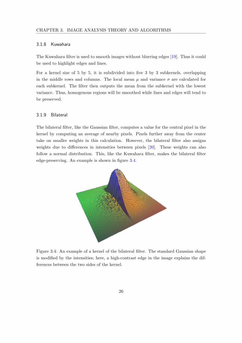
3.1.9 Bilateral

The bilateral filter, like the Gaussian filter, computes a value for the central pixel in the

kernel by computing an average of nearby pixels. Pixels further away from the center

take on smaller weights in this calculation. However, the bilateral filter also assigns

weights due to differences in intensities between pixels [20]. These weights can also

follow a normal distribution. This, like the Kuwahara filter, makes the bilateral filter

edge-preserving. An example is shown in figure 3.4.

Figure 3.4: An example of a kernel of the bilateral filter. The standard Gaussian shape

is modified by the intensities; here, a high-contrast edge in the image explains the dif-

ferences between the two sides of the kernel.

26

CHAPTER 3. IMAGE ANALYSIS THEORY AND ALGORITHMS

The filter is defined as

Ifiltered(x) =1

Wp

∑xi∈Ω

I(xi)fr(‖I(xi)− I(x)‖)gs(‖xi − x‖), (3.11)

with the normalization term

Wp =∑xi∈Ω

fr(‖I(xi)− I(x)‖)gs(‖xi − x‖) (3.12)

where

• Ifiltered is the filtered image;

• I is the original image;

• x are the image coordinates of the current pixel;

• Ω is the kernel centered in x;

• fr is the range Gaussian kernel for smoothing differences in intensities;

• gs is the spatial Gaussian kernel for smoothing differences in intensities.

I used an implementation with constant-time complexity in the experiments [21].

3.2 Algorithm changes for stage 2

Several modifications are added to the algorithms in stage 2. When salt and pepper noise

is added, preprocessing is crucial. This is done by thresholding the image for pixels with

values below a certain, large intensity number. This avoids filtering and ”smearing out”

the many additional high intensity pixels.

When images of the moon and the earth are added, an additional postprocessing step is

needed. This is the exclusion of detected objects larger than a certain size; these objects

are always much bigger than any line in the images.

27

CHAPTER 3. IMAGE ANALYSIS THEORY AND ALGORITHMS

3.3 Complexities

The pixelwise complexities for the different algorithms are seen in table 3.1. For the com-

plexities when processing images, the values are multiplied with the image dimensions

M and N, in addition to other constants depending on the algorithm. These calculations

have to be supplemented with actual execution times and hardware considerations in

order to approximate how feasible implementations of the algorithms would be. This is

shown in section 4.1.

The Mean and Gaussian gradient are separable; this means that the 2D convolutions

can be replaced by two 1D convolutions, significantly reducing computational time. The

Laplacian of Gaussian is not directly separable, but it can be implemented as a sum

of two separable second derivative filters. The median filter’s complexity arises from

the sorting step. The change detection is constant in time because it is not a filter,

meaning there is no kernel. The Canny method is comprised of many steps, the worst

ones being O(n2). The Wiener filter’s complexity arises from the variance calculations.

The nominally lower Kuwahara complexity is because of the of four subkernels.

Table 3.1: The pixel-wise complexities for the tested algorithms. n is the width of a

square kernel.

Algorithm Complexity for each pixel

Mean (separable) O(n)

Median O(n2log(n))

Gaussian Gradient (separable) O(n)

Laplacian of Gaussian (separable) O(n)

Canny O(n)

Change detection O(1)

Wiener O(n2)

Kuwahara O(n2)

Bilateral O(1)

28

Chapter 4

Results

The results for stages 1 and 2 testing are found in sections 4.1 and 4.2, respectively.

4.1 Stage 1

For stage 1 testing, many parameters were tested for each algorithm. Each parameter

setting yielded one set of results. The best of these in terms of sensitivity and specificity

are seen in table 4.1.

Also shown is the execution time for each image, along with a subjective difficulty metric.

This metric incorporates theoretical complexities, execution times and additional con-

straints due to hardware limitations. Most importantly, the change detection algorithm

relies on two frames. Accessing several frames restricts certain hardware setups.

29

CHAPTER 4. RESULTS

Table 4.1: The best results from stage 1 testing. These are for one specific set of pa-

rameters out of all combinations that were tested. Execution time is per image and in

seconds. The difficulty is a subjective metric that assesses how feasible an implemen-

tation would be. It incorporates execution time, theoretical complexity and additional

considerations resulting from hardware limitations.

Algorithm Sensitivity Specificity Execution time Difficulty

Mean 0.67 0.97 0.11 LOW

Median 0.77 0.99 0.71 HIGH

Gaussian Gradient 0.69 1 0.11 LOW

Laplacian of Gaussian 0.99 1 0.14 LOW

Canny 0.94 0.99 0.63 HIGH

Change detection 0.87 1 0.15 HIGH

Wiener 0.99 0.99 0.38 HIGH

Kuwahara 0.57 0.97 2.33 HIGH

Bilateral 0.48 1 14.08 HIGH

4.2 Stage 2

Based on the results of stage 1, The Laplacian of Gaussian algorithm was chosen for

further testing in stage 2. It had almost perfect sensitivity and specificity, while I

assessed its difficulty as relatively low due to its low complexity and fast execution. The

sigma parameter was set to 1.5, with a kernel size of 11x11 pixels. This algorithm also

made use of the modifications presented in section 3.2. The complete version is shown

in section 8.1. Presented below are the results of stage 2 testing. All of the plots have a

”jagged” appearance due to the variance between different images; testing the algorithms

on thousands instead of hundreds of images would rectify this behaviour.

30

CHAPTER 4. RESULTS

4.2.1 Varying line length

The length of the line was varied as shown in figure 4.1. It can be seen that the sensitivity

is high for lengths higher than 50 pixels, and that it drops sharply when the length is

decreased.

Figure 4.1: Varying the length of the line in the images. As the length increases, so does

the sensitivity.

31

CHAPTER 4. RESULTS

4.2.2 Varying line intensity

The intensity factor of the object was varied as shown in figure 4.2. It can be seen that

the sensitivity is high for a factor of 0.95 and higher, and drops rapidly to zero when the

factor is decreased.

Figure 4.2: Varying the intensity factor of the line in the images. As the factor increases,

so does the sensitivity.

32

CHAPTER 4. RESULTS

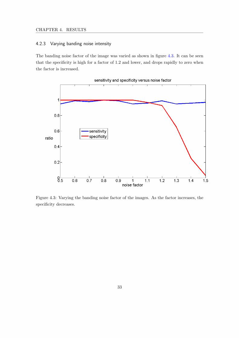
4.2.3 Varying banding noise intensity

The banding noise factor of the image was varied as shown in figure 4.3. It can be seen

that the specificity is high for a factor of 1.2 and lower, and drops rapidly to zero when

the factor is increased.

Figure 4.3: Varying the banding noise factor of the images. As the factor increases, the

specificity decreases.

33

CHAPTER 4. RESULTS

4.2.4 Varying gaussian noise variance

The gaussian noise factor of the image was varied as shown in figure 4.4. It can be seen

that the specificity is high for a variance of 9∗10−5 and lower, and drops rapidly to zero

when the variance is increased.

Figure 4.4: Varying the gaussian noise variance of the images. As the variance increases,

the specificity decreases.

34

CHAPTER 4. RESULTS

4.2.5 Varying salt and pepper noise density

The salt and pepper noise density of the image was varied as shown in figure 4.5. It can

be seen that the specificity is high for a density of 0.01 and lower, and drops rapidly to

zero when the density is increased. The increase in sensitivity for a density of around

0.07 and higher is due to the algorithm incorrectly detecting lines in the noise.

Figure 4.5: Varying the salt and pepper noise density of the images. As the density

increases, the specificity decreases.

35

CHAPTER 4. RESULTS

4.2.6 Earth and moon present

When images of the moon and the earth were added to the images, they were always

detected by the unmodified algorithm. This translated to a specificity of 0. Removing

objects larger than 225 pixels was sufficient to account for these additional objects in

both cases. The sensitivities, specificities and execution times were then the same as

when no additional objects were present.

36

Chapter 5

Discussion

The developed algorithm could be further improved and extended depending on, among

other things, what kind of prior information is available and what precision is needed.

Related subjects are discussed below, along with a possible implementation design.

5.1 Algorithm selection and evaluation

The results show that the Laplacian of Gaussian algorithm performs very well in stage 1

testing, delivering almost perfect sensitivity and specificity for an image of local signal-

to-noise ratio of around 1.32. The execution speed is also among the fastest.

Looking at the results of stage 2 testing, the limitations of the algorithm become ap-

parent. It can be seen from figure 4.1 that the algorithm is fairly robust to decreases

in length, still retaining about 60 % sensitivity for 40 pixels in length. In figure 4.2,

when the line intensity is halved from 0.5 to 0.25, the sensitivity drops to almost 0. In

figure 4.3, when the banding noise is increased by 50 %, the specificity drops to almost

0, meaning many false detections. The same is true when the gaussian noise variance is

increased from 0.00005 to 0.00015, as seen in figure 4.4. This corresponds to an increase

of noise of about 40 %. The algorithm also functions perfectly for a salt-and-pepper

noise with a density up to about 3 %, as seen in figure 4.5.

Whether or not these results are good depends on external specifications on what the

system should be able to handle. If physical characteristics of the RSO to be identified

were set, such as their size, reflectance and distance from the camera, their intensity in

37

CHAPTER 5. DISCUSSION

an image could be modelled. The results from stage 2 testing could also be translated

into limitations on e.g. maximum range or minimum reflectance.

Assume that the RSO parameters would translate into a line of high intensity, meaning

a higher local signal-to-noise ratio. Then the Laplacian of Gaussian algorithm could

probably be replaced with a simpler algorithm, such as the mean filter. This would

improve execution speed without significantly dropping sensitivity.

5.2 Efficiency considerations

Some of the matlab functions that were tested could be replaced by more efficient alter-

natives.

5.2.1 The BWarea function

The BWareaopen function was used in the postprocessing step of all algorithms and

consists of two stages. In the first, connectivity analysis is done by checking each pixel if

it is labelled. If not, it is labelled as a new object, and all pixels in its 8-neighborhood are

also recursively labelled as the same object. In the second stage, the area is calculated

for each object by the BWarea function. This checks each pixel’s 2-by-2 neighborhoods.

There are 4 in total, and each is weighted depending on both the number and distribution

of “on” pixels.

A simpler alternative would be to count the number of pixels in the object. The total

area would then be the sum of all pixels instead of the sum of the BWarea calculations.

A short experiment showed that the area of the lines were around 1.15 % bigger than

those of random noise objects, when comparing the BWarea function with the simple

pixel count. The BWarea function thus results in a slightly higher sensitivity at the cost

of a higher complexity.

5.2.2 Bilateral filter implementation

The algorithm that used a bilateral filter was by far the slowest. The filter could be

replaced with faster variants that, even though they scale poorly with kernel size, have

much lower constants in the complexities. These are typically orders of magnitude faster.

38

CHAPTER 5. DISCUSSION

However, they would still yield the same sensitivity and specificity. Since the resulting

sensitivity was low, an alternative was not pursued.

5.3 Noise and calibration

There are many additional sources of noise that can appear when operating CCD’s and

CMOS devices in space [22]. Some examples of this can be seen in figure 5.1. Bright

columns appear as vertical streaks in the image. Hot spots are pixels with high dark

current, meaning consistently high intensity. Cosmic rays result in temporary clusters

of high intensity. Possible coping strategies include calibration or preprocessing with

low-pass filters to increase the local signal-to-noise ratio.

If noise is fairly consistent across frames, calibration might increase the local signal-to-

noise ratio. For an 8-bit image, this can be done by using pictures of completely dark

and light fields:

Ical = 255 · Iin − IBIW − Iin

(5.1)

where Ical is the calibrated image, Iin is the input image, IB is the dark image and IW

is the light image.

Low-pass filtering in the fourier domain might be an efficient strategy to attenuate

the noise if the bands appear with the same frequencies but different locations in the

images.

39

CHAPTER 5. DISCUSSION

Figure 5.1: Additional noise: Bright columns, cluster of hot spots and cosmic rays.

40

CHAPTER 5. DISCUSSION

5.4 Algorithm extensions

The final algorithm could be improved and extended. This depends on, for example, the

requirements in detection precision and what kind of prior information is available.

5.4.1 Postprocessing using mathematical morphology

Before the postprocessing step of removing small objects with the BWarea function, small

gaps in neighboring objects could be closed. This could be done using mathematical

morphology [16, p. 627]. This would improve the sensitivity of the algorithm, providing

that the true object is made bigger than the false objects in the noise.

5.4.2 Position and speed measurements

When RSO are detected in images, further measurements can be done. The endpoints

of the line can be calculated, and their positions in declination and right ascent can be

determined from star tracker data. If data from several frames are available along with

their time stamps, it is also possible to calculate the change in declination and right

ascent per time unit.

For the position measurements, precision in detecting the endpoints is critical for orbit

determination. Unfortunately, the algorithm will have difficulties separating the end-

points from noise if the local signal-to-noise ratio is poor. Dealing with this problem

is not trivial, but perhaps it could be solved by analyzing image intensity values in the

vicinity of detected pixels.

5.4.3 Several RSO in frame

It might be possible that several RSO enter the frame at once. If this is likely to happen,

additional tracking parameters will become necessary to separate the RSO from each

other. This could be done by, for example, comparing positions and velocities of the

lines from the previous frames with the current one.

41

CHAPTER 5. DISCUSSION

5.5 Implementation

To put the algorithm to work aboard spacecraft, the matlab algorithm will need to be

translated to a star tracker computer architecture. I investigated the AAC Microtec

star tracker as a model. It is subdivided into the two layers of RTL (register transfer

level), and software. The RTL is very low-level, and uses languages such as Verilog and

VHDL. These are very efficient, but it is difficult to implement complex algorithms. The

software level typically uses the C programming language.

One example setup would be to do the preprocessing in RTL, and the rest of the al-

gorithm in software. For the C language, the openCV library could be used for its

implementations of common image processing functions such as the Laplacian of Gaus-

sian filter. It is not clear if this model architecture is sufficiently powerful for full-scale

image processing, which is needed for this application.

42

Chapter 6

Orbit determination

Consider figure 6.1. One RSO is detected in three separate images in sequence from left

to right. From the image it is unclear if the RSO is moving away from the observer or

towards it. However, the angular positions of the endpoints of the detected lines can be

calculated. Combining this information with the constraints of orbital motion and the

positions of the observer at the times of observations, a preliminary orbit of the RSO

can be computed.

Figure 6.1: Three exposures of an RSO passing by in the camera’s field of view. The

images are in sequence from left to right.

43

CHAPTER 6. ORBIT DETERMINATION

An example of how to do this with the Gaussian angles-only method is discussed below,

along with possible limitations of this approach. It is important to note that this is

only one of the angles-only methods available; others include the Laplacian method, the

Double R method, and the Gooding method [23]. Only the Gauss method is considered

because of its good performance for observations which are close together [24, p. 14].

However, other methods might be more precise depending on, among other factors, the

type of orbits encountered.

6.1 Ground-based Gaussian angles-only method

The ground-based Gaussian angles-only method relies on three angular measurements of

the RSO. Also needed are the times of the measurements and the position on the earth’s

surface of the observer.

An overview of the situation can be seen in figure 6.2. Using a geocentric coordinate

system, the vectors r correspond to the positions of the RSO. The vectors R correspond

to the known positions on the earth, which change in time due to the rotation of the

earth. The vectors α correspond to the positions of the RSO relative to the positions

on the earth. The unit vectors α are known from the angular measurements, but the

ranges α are unknown. All of the vectors correspond to the known times t1, t2 and t3

respectively.

We want to determine r2 and v2, the velocity vector of the RSO at time t2. The orbital

parameters can then be determined using standard calculations [25, p. 159].

From figure 6.2, it is evident we have the following equation system:

r1 = R1 +α1

r2 = R2 +α2

r3 = R3 +α3

(6.1)

meaning 9 scalar equations and 12 unknowns (the nine components of the r vectors and

the three ranges α).

Due to conservation of angular momentum and the Keplerian orbit, the r vectors must

be in the same plane. It can be shown that r2 is a linear combination of r1 and r3:

r2 = c1r1 + c3r3 (6.2)

44

CHAPTER 6. ORBIT DETERMINATION

Now we have 12 scalar equations and 14 unknowns.

Another consequence of the Keplerian two-body equation of motion is that the state

vectors r and v at one time can be expressed using the state vectors at any other given

time. This is done using Lagrange coefficients, resulting in the following equations:

r1 = f1r2 + g1v2

r3 = f3r2 + g3v2(6.3)

It can be shown that if the time intervals between the tree observations are sufficiently

small, the coefficients f and g only depend on the center of attraction r2. Thus, we have

six new scalar equations and four new unknowns: the three components of v2 and the

radius r2. Finally we have a well-posed system of 18 equations and 18 unknowns. For a

complete derivation of the system and its solution, see [25, p.236].

45

CHAPTER 6. ORBIT DETERMINATION

r₁

R₁

α₁

α₂

α₃

r₂

r₃

R₃ R₂

Figure 6.2: The system of vectors when using a geocentric coordinate system. The angles

of the RSO are measured from the earth. The red object is an RSO and the black object

is a known position on earth rotating with the earth. The vectors correspond to the

known times (t1, t2 and t3) respectively. Note that the orbit may be elliptic instead of

circular.

46

CHAPTER 6. ORBIT DETERMINATION

r₁

R₁

α₁

α₂

α₃

r₂

r₃

R₃ R₂

Figure 6.3: The system of vectors when using a geocentric coordinate system. The

angles of the RSO are measured from a star tracker aboard a satellite. The red object

is an RSO and the black object is the satellite doing the measurements. The vectors

correspond to the known times (t1, t2 and t3) respectively. Note that both orbits may

be elliptic instead of circular.

47

CHAPTER 6. ORBIT DETERMINATION

6.2 Satellite-based Gaussian angles-only method

In this case, we want to do orbit determination from data using a star tracker aboard

an observing satellite. Thus, the R variables are the geocentric positions of the orbiting

observing satellite. This is seen in figure 6.3. In all other respects the procedure is

identical to the one in section 6.1.

6.3 Limitations

This approach of preliminary orbit determination is subject to several limitations. First,

we need the positions of the observing satellite at specific times. It could either be

measured directly or calculated from its orbital data. Regardless, the position will

probably be imprecise to some extent.

Secondly, we need three angular positions of the RSO. The detection algorithm will

need a high sensitivity and specificity. The detected angular positions will suffer from

low precision if the local signal-to-noise ratio is low. The solution of the orbit determi-

nation equations rely on approximations and numerical techniques, introducing further

imprecision.

It is possible that the RSO will be visible as a curve instead of a straight line. In that

case, its shape contains information about its orbit. By only comparing the endpoints

of the line, much of this information is wasted.

These limitations probably mean low precision in the preliminary orbit determination.

However, the orbital data could be refined if more measurements were available. This

could be done by using statistical methods [26].

6.4 Implementation

The solution of the equations is divided into many steps encompassing algebra, linear

algebra and numerical root finding. Each step by itself is not very computationally

intense when compared to image filtering. If the computer architecture is sufficiently

powerful to do the detection algorithm, it should also be able to do the initial orbit

determination.

48

Chapter 7

Conclusions and further research

For images taken with star trackers, the presence of resident space objects can be detected

using image analysis algorithms. Their angular positions in declination and right ascent

can also be determined. This data can be used to do an imprecise preliminary orbit

determination with the Gaussian angles-only method. Three measurements with small

time differences are needed, combined with the times of detection and the positions of

the observing satellite.

The detection algorithm should be adjusted and calibrated depending on the expected

intensity of the RSO to be detected and the type of noise. If specifications about the

RSO were available, such as the reflectance, the distance from the camera and the inte-

gration time, their line intensities could be modelled. The noise could also be modelled

depending on sensors, optics and operational requirements. For lines with low local

signal-to-noise ratio, the detection algorithm should be based on the Laplacian of Gaus-

sian filter. For lines with high local signal-to-noise ratio, a less computationally intense

algorithm could be used. If the local signal-to-noise ratio is very low, all of the tested

algorithms’ sensitivities will be very low. More sophisticated methods, which are much

more computationally intense, might perform better.

It is difficult to say how technically feasible the solution is. In terms of computational

intensity, the bottleneck should be the image analysis. The Laplacian of Gaussian filter

is separable but requires a fairly large kernel size. The orbit determination calculations

should be less costly. Thus, a computer architecture capable of image processing is

needed for an onboard implementation. Considering the power, size, weight and evolu-

tion of modern smartphones, this problem should be possible to solve [27].

49

Chapter 8

Appendix

8.1 The final algorithm

Presented below is the final algorithm implemented in a matlab function. It is not

optimized. The input is the raw image. The output is the binary image of detected

objects, together with a detection boolean. The algorithm is divided into three parts:

preprocessing, main, and postprocessing.

The pre-processing is optional in case of heavy salt and pepper noise. High intensity

pixels are set to zero in order to avoid ”smearing out” the pixels. If this is not done, the

specificity drops as many objects are falsely detected in the noise.

In the main part, the Laplacian of Gaussian kernel is constructed. Its size and shape is

controlled by the sigma parameter. Then, the image is filtered. The resulting image is

thresholded to produce a binary image of detected objects. Connectivity analysis and

labelling of different objects is made with the BWareaopen function. Small objects are

removed in the process. Optionally, large objects are removed as well. This takes care

of falsely detected objects such as the moon or the earth.

In the postprocessing step, the edges are removed. This is done because the edges always

contain false hits due to limitations in the hardware. Finally, the image is checked for

any remaining on pixels. If there are any, the function returns a positive detection.

50

CHAPTER 8. APPENDIX

Data: Raw 8-bit image (ImIn)

Result: Detection output (boolean) and binary image ImOut

function [detected, ImOut] = LoGFilter(ImIn)

%% Preprocessing

% Optional: Preprocess image to remove bright pixels

ImIn = uint8(uint8(ImIn<50).*ImIn);

%% Main part

% Choose sigma value, calculate size of kernel and construct LoG kernel

sigma = 1.5;

cutoff = ceil(3*sigma);

h = fspecial(’log’, 2*cutoff+1, sigma);

% Filter image

ImFiltered = conv2(ImIn,h,’same’);

% Threshold image (choose parameter wisely)

ImThresholded = ImFiltered < - 0.5;

% Do connectivity analysis and remove small objects, and, optionally, large objects.

ImOut = bwareaopen(ImThresholded, 35) - bwareaopen(ImThresholded, 225);

%% Postprocessing

% Remove edges

ImOut(1:20,:) = 0;

ImOut(:,1:20) = 0;

ImOut(972-20:972,:) = 0;

ImOut(:,1296-20:1296) = 0;

% Output true if any object remains.

hits = sum(sum(ImOut));

if (hits > 0);

detected = true;

else

detected = false;

end

51

Bibliography

[1] BBC, “In orbit: How satellites rule our world,” 2013.

[2] The Economist, “Nanosats are go!.” http://www.economist.com/news/

technology-quarterly/21603240-small-satellites-taking-advantage-

smartphones-and-other-consumer-technologies. Accessed: 2014-08-19.

[3] NASA, “Orbital debris faq.” http://orbitaldebris.jsc.nasa.gov/faqs.html.

Accessed: 2014-08-19.

[4] Christer Andersson, Lisa Rosenqvist, Eva Bernhardsdotter, Mats Persson, “SSA -

Behover Sverige en rymdlagesbild?,” Swedish Defence Research Agency, 2011.

[5] A. E. Roy, Orbital Motion, Fourth Edition. Taylor & Francis Group, 2005.

[6] Simon Sze and Ming-Kwei Lee, Semiconductor devices, physics and technology, third

edition. Wiley, 2013.

[7] Photometrics.com, “Dark current.” http://www.photometrics.com/resources/

learningzone/darkcurrent.php. Accessed: 2014-08-19.

[8] NASA jet propulsion laboratory, “St6 star camera.” http://nmp.jpl.nasa.gov/

st6/TECHNOLOGY/star_camera.html. Accessed: 2014-08-19.

[9] Milan Sonka, Vaclav Hlavac, Roger Boyle, Image Processing, Analysis, and Machine

Vision - Third Edition. Cengage Learning, 2008.

[10] Centrum for bildanalys, Sveriges lantbruksuniversitet, Uppsala universitet, “Intro-

duktion till datoriserad bildanalys.” http://www.cb.uu.se/baintro/index.html.

Accessed: 2014-08-19.

[11] Stephen J. Battazzo, “Development of a star sensor based attitude determination

system for microsatellites,” Master’s thesis.

52

BIBLIOGRAPHY

[12] Smithsonian Astrophysical Observatory, “SAO Star Catalog.” http://tdc-www.

harvard.edu/catalogs/sao.html. Accessed: 2014-09-01.

[13] Wolfram Mathworld, “Gnomonic projection.” http://mathworld.wolfram.com/

GnomonicProjection.html. Accessed: 2014-09-01.

[14] Digital Photo Pro, “Noise: Lose it, part ii.” http://www.digitalphotopro.

com/technique/revolution/noise-lose-it-part-ii.html#.U_3pKrt_W5l. Ac-

cessed: 2014-09-01.

[15] A.G. Lalkhen, A. McCluskey, “Clinical tests: sensitivity and specificity,” Continu-

ing Education in Anasthesia, Critical Care & Pain, 2008.

[16] Rafael C. Gonzales, Richard E. Woods, Digital image Processing - Third Edition.

Pearson Education, 2008.

[17] Cris L. Luengo Hendriks, “Gaussian filtering.” http://www.cb.uu.se/~cris/

blog/index.php/archives/22. Accessed: 2014-09-15.

[18] Lim, Jae S, Two-Dimensional Signal and Image Processing. Prentice Hall, 1990.

[19] Giuseppe Papari, Nicolai Petkov, Patrizio Campisi, “Artistic edge and corner en-

hancing smoothing,” IEEE Transactions on Image Processing, 2007.

[20] Carlo Tomasi, Roberto Manduchi, “Bilateral filtering for gray and color images,”

Sixth International Conference on Computer Vision, 1998.

[21] Kunal Narayan Chaudhury, Daniel Sage, Michael Unser, “Fast O(1) Bilateral Filter-

ing Using Trigonometric Range Kernels,” IEEE Transactions on Image Processing,

2011.

[22] European Southern Observatory, “CCD noise.” http://www.eso.org/~ohainaut/

ccd/CCD_artifacts.html. Accessed: 2014-10-02.

[23] Andrew Vernon Schaeperkoetter, “A comprehensive comparison between angles-

only initial orbit determination techniques,” Master’s thesis, Texas A&M University,

2011.

[24] David C. Woffinden, Angles-only Navigation for Autonomous Orbital Rendezvous.

PhD thesis, Utah State University, 2008.

[25] Howard Curtis, Orbital Mechanics for Engineering Students. Elsevier, 2005.

53

BIBLIOGRAPHY

[26] Bob Schutz, Byron Tapley, George Born, Statistical Orbit Determination. Elsevier,

2004.

[27] NASA Ames’ Smartphone Nanosatellite, “PhoneSat.” www.phonesat.org. Ac-

cessed: 2014-10-22.

54