HAL Id: hal-03153901https://hal-centralesupelec.archives-ouvertes.fr/hal-03153901

Submitted on 26 Feb 2021

HAL is a multi-disciplinary open accessarchive for the deposit and dissemination of sci-entific research documents, whether they are pub-lished or not. The documents may come fromteaching and research institutions in France orabroad, or from public or private research centers.

L’archive ouverte pluridisciplinaire HAL, estdestinée au dépôt et à la diffusion de documentsscientifiques de niveau recherche, publiés ou non,émanant des établissements d’enseignement et derecherche français ou étrangers, des laboratoirespublics ou privés.

Detecting Ephemeral Objects in SAR Time-Series UsingFrozen Background-Based Change DetectionThibault Taillade, Laetitia Thirion-Lefevre, Régis Guinvarc’H

To cite this version:Thibault Taillade, Laetitia Thirion-Lefevre, Régis Guinvarc’H. Detecting Ephemeral Objects in SARTime-Series Using Frozen Background-Based Change Detection. Remote Sensing, MDPI, 2020, 12(11), pp.1720. �10.3390/rs12111720�. �hal-03153901�

remote sensing

Article

Detecting Ephemeral Objects in SAR Time-SeriesUsing Frozen Background-Based Change Detection

Thibault Taillade *, Laetitia Thirion-Lefevre and Régis Guinvarc’h

SONDRA, CentraleSupélec, Université Paris-Saclay, 3 Rue Joliot Curie, 91190 Gif-sur-Yvette, France;laetitia.thirion@centralesupelec.fr (L.T.-L.); regis.guinvarch@centralesupelec.fr (R.G.)* Correspondence: thibault.taillade@centralesupelec.fr

Received: 24 April 2020; Accepted: 21 May 2020; Published: 27 May 2020�����������������

Abstract: Change detection (CD) in SAR (Synthethic Aperture Radar) images has been widelystudied in recent years and has become increasingly attractive due to the growth of available datasets.The potential of CD has been shown in different fields, including disaster monitoring and militaryapplications. Access to multi-temporal SAR images of the same scene is now possible, and thereforewe can improve the performance and the interpretation of CD. Apart from specific SAR campaignmeasurements, the ground truth of the scene is usually unknown or only partially known whendealing with open data. This is a critical issue when the purpose is to detect targets, such as vehiclesor ships. Indeed, typical change detection methods can only provide relative changes; the actualnumber of targets on each day cannot be determined. Ideally, this change detection should occurbetween a target-free image and one with the objects of interest. To do so, we propose to benefitfrom pixels’ intrinsic temporal behavior to compute a frozen background reference (FBR) image andperform change detection from this reference image. We will then consider that the scene consists onlyof immobile objects (e.g., buildings and trees) and removable objects that can appear and disappearfrom acquisition to another (e.g., cars and ships). Our FBR images will, therefore, aim to estimatethe immobile background of the scene to obtain, after change detection, the exact amount of targetspresent on each day. This study was conducted first with simulated SAR data for different numberof acquisition dates and Signal-to-Noise Ratio (SNR). We presented an application in the region ofSingapore to estimate the number of ships in the study area for each acquisition.

Keywords: change detection; time-series; SAR; target detection

1. Introduction

SAR (Synthetic Aperture Radar) images change detection is a promising solution for targetdetection when dealing with high cluttered environments, such as urban areas, forests, or harbors.Indeed, typical CFAR (Constant False Alarm Rate) detectors computed on single images also providethe scatterers that belong to the background and can fail to detect targets due to the high clutter levelrelative to the target response [1].

SAR images change detection (CD) has been widely studied, for instance, in bi-date cases andfor multi-temporal data in [2,3]. Typical bi-date based change detection approaches represent arelative change between the combination of acquisitions. As such, it might lead to misinterpretation,for example, if the target was present during the two acquisitions or when a target overlaps on twodifferent dates. Such processing implies that, for every new image acquired, the algorithm needs to berecomputed on the whole time-series.

In the case of multi-temporal change detection, previous works detected the most significantchange that occurred during the time series with knowledge of the change point as in [4]. However,in dense activity areas, such as industrial harbor or parking, several objects can overlap in the

Remote Sens. 2020, 12, 1720; doi:10.3390/rs12111720 www.mdpi.com/journal/remotesensing

Remote Sens. 2020, 12, 1720 2 of 21

time domain and cannot be highlighted with such methods. We propose here to introduce a newchange detection framework based on the computation of a frozen background reference (FBR) image,taking into account the multi-temporal capabilities of the new sensors. To do so, we consider that ascene consists of two classes of objects: ephemeral objects (targets that can move from one acquisitionto another, such as cars) and immovable objects (e.g., trees and buildings).

First, several aspects of multi-temporal SAR will be discussed. Afterward, the computation of thisFBR image will be detailed, and the statistical properties of such images will be studied. The objectiveis to identify the stable part of each pixel within the temporal domain and generate the FBR image.We propose to achieve this through the use of a time variation coefficient. Thus, a list of stable candidatepixels was built and used for change detection. This approach was tested first on simulated complexGaussian images and then on real SAR image configurations, and results are presented for the detectionof ephemeral objects in the context of maritime surveillance.

2. Multitemporal Change Detection

Remote Sensing is increasingly attractive to the scientific community as well as to governmentalinstitutions in different domains. Several SAR times series are currently available, and even more willbe in open access in the future [5,6]. Therefore, it is essential to develop methodologies and concepts todeal with this critical amount of data and extract the information in our interest. The CD between twodates has been thoroughly studied [7]; the associated statistics related have been derived in the past.For a few years, the amount of open data acquired periodically has been increasing and provides alarge amount of data that has to be processed automatically depending on the application and needsof users. MCD (multitemporal change detection) has been as well studied. Statistical tests have beenderived in two different forms: a multi-bidate detection that can provide information on the numberof changes within the time series, or another form that provides binary information over the wholetime series.

2.1. Multi-Bidate Detection Approach

This framework of change detection introduced by [3] performs a bi-date CD sequentially orcombinatorially (all possible dates combinations). Then the output results represent different classesaccording to the sum of changes or the possible combination of changes occurring within the time-series.We present the representation of such a framework in Figure 1.

Figure 1. Multi bi-date change detection.

This method, however, does not consider the temporal statistics of the pixels since they arecomputed for a bi-date combination. It is not possible to retrieve the current ephemeral objects at aspecific date because it is a relative procedure. Finally, for each new acquisition, the whole dataset hasto be recomputed, increasing the computational cost.

2.2. Variation Coefficient Based CD

The variation coefficient (CV), also known as the relative standard deviation, is mathematicallydefined in probability theory and statistics by σ/µ, where σ is the standard deviation of the signal and

Remote Sens. 2020, 12, 1720 3 of 21

µ the mean value. It can be considered as a normalized measurement of the dispersion of a probabilitydistribution. A thorough study can be found in [4].

In radar images, it is commonly accepted that the amplitude of a speckle without texture followsthe Rayleigh–Nakagami law:

RN[µ, L](u) =2√

LµΓ(L)

(√Luµ

)2L−1

e−(√

Lµ u)2

(1)

where µ is a form parameter, Γ is the gamma function, and L is called the looks number. In ourapproach, we are interested in time statistics.

According to [4], we can write the theoretical variation coefficient as follows:

CV =

√Γ(L)Γ(L + 1)

Γ(L + 12 )

2− 1. (2)

This expression shows that the coefficient of variation has the same value for all stable specklezones, whatever the average amplitude of this speckle. Also, the variance of the CV decreases with avariation in

√D, with D being the number of dates of the time-series.

2.3. Electromagnetical and Statistical Stability

The concept of electromagnetic stability can be expressed by a high coherence of a deterministicscatterer within the time series, usually known as permanent scatterer (PS) in interferometry.The related temporal variation coefficient is then low, and the coherence between two acquisitions issupposedly high. However, the coherence in low-intensity areas (roads, plane surfaces, and shadows)is also low, giving no further information about the temporal stability of such areas. In the case of astable speckle, the related variation coefficient is also low, but it does not necessarily have a coherenttemporal behavior in the electromagnetic point of view. It is said to be statistically stable becausethe parameter of its probability density function does not vary with time. The temporal variationcoefficient then gives us the opportunity to obtain both electromagnetically and statistically stablepixels within the time series.

In the case of vehicle detection, it can be a keen interest for the user to know at a specific datehow many targets were present in a scene, for example, for harbor monitoring or ground surveillanceapplications. The purpose of remote sensing is to provide images of ground scenes without the needfor a physical presence; however, as the main drawback, we cannot know precisely the state of a sceneat a specific date. As the ground truth is usually unknown, a CD strategy with two dates becomesdifficult to establish because the content of both images remains unknown. The main idea of thismethod is to extract a stable temporal pattern of a scene to build its ground truth blindly: the scene iscomposed of all immobile objects that are electromagnetically or statistically stable in time. Afterward,each image of the scene is compared with this reference scene through change detection algorithms.

3. Frozen Background Reference Image from a Temporal Stack of Radar Images

The study aims to compute the FBR image consisting only of the signature of immovable objectsand speckle noise. We want to obtain all the temporal pixels that are electromagnetically or statisticallystable within the time series. This reference image is used afterward for change detection on a stack ofSAR images. The resulting complex image is said to be a reference image because it aims to represent atarget-free scene with only background pixels stable in time. The concept for such a reference imageis presented in Figure 2. The proposed framework of change detection relies on a simple hypothesis.Within a SAR time-series, it is more likely that a given pixel stays temporally unoccupied by anephemeral object; if not, it is considered as a background object.

Remote Sens. 2020, 12, 1720 4 of 21

SAR TimeSeries

Frozen backgroundimage estimation

ChangeDetection

Figure 2. Frozen background reference (FBR) based change detection (CD) using Synthetic ApertureRadar (SAR) time-series.

3.1. Computation of the FBR Image

We define S as the matrix for a full polarization SAR image. We note i and j as the range andazimuth indices. For D acquisition dates, we note the temporal matrix X = [S(1)...S(D)]. The variationcoefficient CV(Xi,j) is then computed iteratively over each pixel of this temporal matrix in order toextract its stable behavior. At each iteration m, we obtain a new output matrix X̃m

i,j with D′ < D datesconsisting only of pixels representing stable temporal behavior. Figure 3 presents the diagram used toperform such a process.

Figure 3. Candidate pixel selection within the time-series.

At the end of the process, we obtain a cube with an inhomogeneous dimension in the timedirection with only selected stable candidate pixels for each range and azimuth. We illustrate suchresults in the Figure 4. Since the stable candidate pixels of the time series have been chosen, we canassume that any random pixel of the list can be taken as a stable background pixel. This image canbe computed differently depending on the situation. For instance, it is possible to create an FBR

Remote Sens. 2020, 12, 1720 5 of 21

image with only random pixels of the remaining candidate pixels or by taking the mean of theseremaining pixels.

Figure 4. Inhomogenous dimensions in time direction of candidate pixels.

3.2. CV Threshold Computation

As presented in Section 2.2, the theoretical variation coefficient depends only on L (the numberequivalent of look) that can be estimated as proposed in [8]. It can be as well used directly accordingto the SAR acquisition for sentinel 1 GRD product L = 4.9. As discussed, the variance of the CV is afunction of 1√

(D)with D being the number of dates in the time series. The threshold is then defined

using the theoretical variation coefficient in Equation (2):

Ψm(i, j) = CV +α√

Dm(i, j)(3)

where α is a parameter to control the probability of false alarm (PFA) and Dm(i, j) is the remainingnumber of stable dates for each range i and azimuth j at the iteration m. The threshold can be setindependent of the number of the remaining images by choosing α = 0.

3.3. Strategies of Change Detection for Different Computation Modes of the FBR Image

Depending on the computation, it is possible to obtain the FBR image, whether from the coherentmean of each remaining candidate pixels or a single temporal random pixel for each azimuth and range.

3.3.1. Random Pixels

We chose first to select a random pixel from the list of temporal stable candidate pixels for eachazimuth and range of the image. We obtained, therefore, our FBR image X̃(RP). Assuming that thestatistics of speckle remained unchanged, in the space domain (range, azimuth) as well as in the timedomain, we can adapt the different tests introduced in [2]. For classical change detection, we assumethat the pixels of the FBR Image X̃(RP) and the Mission Image Y follow a multivariate zero-meancomplex Gaussian distribution with Cre f and CY as the covariance matrices associated to vectors X̃(RP)

and Y [2]. The test to be computed and compared with a threshold and can be written using thefollowing equation:

γRP =|Cre f |N |CY |N

| 12 (Cre f + CY )|2N(4)

Remote Sens. 2020, 12, 1720 6 of 21

where N is the number of samples within the averaging box to compute the covariance matrix, and ||represents the determinant of the matrix.

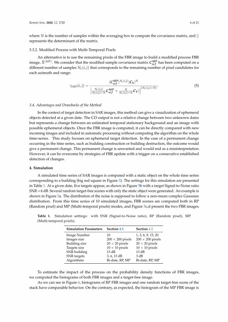
3.3.2. Modified Process with Multi-Temporal Pixels

An alternative is to use the remaining pixels of the FBR image to build a modified process FBRimage, X̃(MP). We consider that the modified sample covariance matrix CMP

re f has been computed on adifferent number of samples Nc(i, j) that corresponds to the remaining number of pixel candidates foreach azimuth and range:

γMP(i, j) =|CMP

re f |Nc(i,j)|CY |N∣∣∣ Nc(i,j)

Nc(i,j)+N CMPre f + N

Nc(i,j)+N CY )∣∣∣(Nc(i,j)+N)

. (5)

3.4. Advantages and Drawbacks of the Method

In the context of target detection in SAR images, this method can give a visualization of ephemeralobjects detected at a given date. The CD output is not a relative change between two unknown datesbut represents a change between an estimated temporal stationary background and an image withpossible ephemeral objects. Once the FBR image is computed, it can be directly compared with newincoming images and included in automatic processing without computing the algorithm on the wholetime-series. This study focuses on ephemeral target detection. In the case of a permanent changeoccurring in the time series, such as building construction or building destruction, the outcome wouldgive a permanent change. This permanent change is unwanted and would end as a misinterpretation.However, it can be overcome by strategies of FBR update with a trigger on a consecutive establisheddetection of changes.

4. Simulation

A simulated time series of SAR images is computed with a static object on the whole time seriescorresponding to a building (big red square in Figure 5). The settings for this simulation are presentedin Table 1. At a given date, five targets appear, as shown in Figure 5b with a target Signal-to-Noise ratioSNR = 6 dB. Several random target-free scenes with only the static object were generated. An example isshown in Figure 5a. The distribution of the noise is supposed to follow a zero-mean complex Gaussiandistribution. From this time series of 10 simulated images, FBR scenes are computed both in RP(Random pixel) and MP (Multi-temporal pixels) modes, and Figure 5c,d present the two FBR images.

Table 1. Simulation settings: with SNR (Signal-to-Noise ratio), RP (Random pixel), MP(Multi-temporal pxiels).

Simulation Parameters Section 4.1 Section 4.2

Image Number 10 1, 3, 6, 9, 15, 20Images size 200 × 200 pixels 200 × 200 pixelsBuilding size 20 × 20 pixels 20 × 20 pixelsTargets size 10 × 10 pixels 10 × 10 pixelsSNR building 13 dB 13 dBSNR targets 3, 6, 13 dB 3 dBAlgorithms Bi-date, RP, MP Bi-date, RP, MP

To estimate the impact of the process on the probability density functions of FBR images,we computed the histograms of both FBR images and a target-free image.

As we can see in Figure 6, histograms of RP FBR images and one random target-free scene of thestack have comparable behavior. On the contrary, as expected, the histogram of the MP FBR image is

Remote Sens. 2020, 12, 1720 7 of 21

squeezed because the variance decreases with a factor√

D, with D being the number of remainingstable dates.

(a) Only building (b) Building and five targets

(c) FBR Scene RP (d) FBR Scene MPFigure 5. Simulated scenes and associated reference images.

Figure 6. Histogram of radiometric scene, MP and RP FBR images.

FBR images were computed, and we will now present the behavior of the change detectionresults between images with target and the FBR images compared with classical bi-date changedetection. The Table 1 presents the different settings used to evaluate the CD results in paragraphSections 4.1 and 4.2.

Remote Sens. 2020, 12, 1720 8 of 21

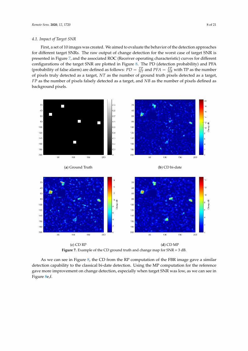
4.1. Impact of Target SNR

First, a set of 10 images was created. We aimed to evaluate the behavior of the detection approachesfor different target SNRs. The raw output of change detection for the worst case of target SNR ispresented in Figure 7, and the associated ROC (Receiver operating characteristic) curves for differentconfigurations of the target SNR are plotted in Figure 8. The PD (detection probability) and PFA(probability of false alarm) are defined as follows: PD = TP

NT and PFA = FPNB with TP as the number

of pixels truly detected as a target, NT as the number of ground truth pixels detected as a target,FP as the number of pixels falsely detected as a target, and NB as the number of pixels defined asbackground pixels.

(a) Ground Truth (b) CD bi-date

(c) CD RP (d) CD MPFigure 7. Example of the CD ground truth and change map for SNR = 3 dB.

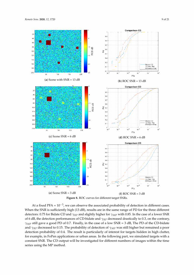
As we can see in Figure 8, the CD from the RP computation of the FBR image gave a similardetection capability to the classical bi-date detection. Using the MP computation for the referencegave more improvement on change detection, especially when target SNR was low, as we can see inFigure 8e,f.

Remote Sens. 2020, 12, 1720 9 of 21

(a) Scene with SNR = 13 dB (b) ROC SNR = 13 dB

(c) Scene SNR = 6 dB (d) ROC SNR = 6 dB

(e) Scene SNR = 3 dB (f) ROC SNR = 3 dBFigure 8. ROC curves for different target SNRs.

At a fixed PFA = 10−3, we can observe the associated probability of detection in different cases.When the SNR is sufficiently high (13 dB), results are in the same range of PD for the three differentdetectors: 0.75 for Bidate CD and γRP and slightly higher for γMP with 0.85. In the case of a lower SNRof 6 dB, the detection performances of CD-bidate and γRP decreased drastically to 0.3, on the contrary,γMP still gave a good PD of 0.7. Finally, in the case of a low SNR = 3 dB, The PD of the CD-bidateand γRP decreased to 0.15. The probability of detection of γMP was still higher but remained a poordetection probability of 0.4. The result is particularly of interest for targets hidden in high clutter,for example, in FoPen applications or urban areas. In the following part, we simulated targets with aconstant SNR. The CD output will be investigated for different numbers of images within the timeseries using the MP method.

Remote Sens. 2020, 12, 1720 10 of 21

4.2. Impact of the Number of Available Dates

To evaluate the benefit of using several dates for the computation of the FBR scenes, several changemaps were produced using the simulated ground truth with different amounts of images randomlychosen from the simulated SAR stack. The results are shown in Figure 9a,b. We can observe that thedetection was improved when increasing the number of dates taken as a reference.

(a) ROC curve linear PFA (b) ROC curve (semilog)Figure 9. ROC (Receiver Operating Characteristic) curves representing PD (probality of detection) andPFA (probabiblity of false alarm) for different amounts of images used to create the FBR scene.

4.3. Polarimetric Case

In this part, we present the results with the framework used in the case of polarimetric data sothat channels HH, HV, and VV (H stands for Horizontal and V for Vertical) will be gathered in onepolarimetric vector. The process proposed in 3.1 was performed on each channel independently, and anew reference polarimetric vector was composed. We present the result in Figure 10.

(a) ROC curve (linear PFA) (b) ROC curve (semilog)Figure 10. ROC (Receiver Operating Characteristic) curves for polarimetric vectors.

From this simulation study, we can conclude on different aspects of the method. First, the choiceof a random pixel RP within the candidate pixels from simulation gave comparable results to a typicalbi-date detection. However, the interpretation of CD results was improved as only the ephemeralobjects are seen in the resulting image. Considering the use of all remaining candidate pixels throughthe MP method, we can see that the detection capability was drastically better when the target SNRwas decreasing. This property was a promising result for the detection of targets hidden in a highcluttered environment.

Remote Sens. 2020, 12, 1720 11 of 21

5. Results on Real SAR Data

As an illustration, a scene with boats (floating platform) on water was chosen to test our approach.A second, more complex example was selected in an industrial harbor area near Singapore.

5.1. Floating Platform over a Lake in the Area of San Francisco

This example focuses on floating platforms over sea surfaces that can have different configurations,as shown in Figure 11. The characteristics of the images used for the study are presented in Table 2.

Table 2. UAVSAR (Uninhabited Aerial Vehicle Synthetic Aperture Radar) data acquisitionscharacteristics used for the study.

Technical Characteristics of the Sentinel Images

Acquisition Mode PolSARProcessing level Single Look Complex (SLC)Polarisation (HH+HV+VH+VV)Resolution 1.8 × 0.8 mWavelength L-BandStack Name SDelta_23518_01Acquisition dates June 2009 to June 2010Location https://www.google.com/maps/search/?api=1&query=38.052500001,-121.83250000

(a) Configuration 1 (b) Configuration 2

Figure 11. Example of floating platforms over this lake, seen on Google Earth images.

The scene under study is composed of 12 L-band fully polarimetric UAVSAR (Uninhabited AerialVehicle Synthetic Aperture Radar) images in the region around San Francisco. Figure 12a is the firstradiometric HH image of the temporal stack, and Figure 12b,c are the FBR images obtained from ourmethod using the RP and MP methods. The images are represented in gray levels from −30 to 0 dB.

(a) Radiometric 1 HH (b) FBR-RP (c) FBR-MPFigure 12. Radiometric UAVSAR image and MP and RP reference images.

As we can observe in this reference image, the targets were successfully removed. Figure 13apresents the results of the usual change detection between two dates of the stack. Red values on the

Remote Sens. 2020, 12, 1720 12 of 21

image indicate that a significant change of amplitude occurred, whereas blue areas reflect areas withno changes.

Floating platforms were present at both dates, but not precisely in the same position;thus, the resulting image was difficult to interpret. In Figure 13b–e we plotted the results of changedetection from the FBR images in RP and MP modes and the two dates that were used previously forthe classical bi-date change detection. In both results, we can directly see a better quality for the image,and it is possible to more accurately identify the targets present at each date. In that case, the SNR ofthe boat was high; therefore, the results in RP and MP modes were similar as they are presented in thesimulation of a high SNR target. This example shows that it is possible to use this method in the caseof target detection, especially when it is necessary to know the number of targets present on one imagewithout knowledge of the scene. As we can also notice, the signal to noise ratio was improved, and thetargets were more easily identifiable.

(a) CD Bidate 1 and 2 (b) CD RP date 1 (c) CD RP date 2

(d) CD MP date 1 (e) CD MP date 2Figure 13. CD results for RP and MP modes.

5.2. Singapore Region Study

A more complex area was chosen in Singapore in the industrial harbor of Jurong Island. Figure 14shows the FBR image computed using 83 Sentinel GRD (Ground Range Detected) Images of Singaporeprojected on Google Earth in order to validate the reference scene. The characteristics of the Sentineldata used in this study can be found in Table 3. In addition, the Figure A2 represents the operationsperformed for each GRD image of the stack. The stack was afterward coregistrated according to thefirst image of the stack using the function «Coregistration» of SNAP (Sentinel Application Platform)software [9]. Since the environment is constituted of man-made structures, we chose to use SARimages with always the same configuration of observation, and thus the same orbit number. Indeed,most man-made structures cannnot be considered to possess an azimuthal symmetry and a subtlechange in the observation angle can drastically affect their back-scattered signals. Using differentorbits to compute the FBR image might corrupt the estimation of the stable background.

Remote Sens. 2020, 12, 1720 13 of 21

Table 3. Sentinel 1 data acquisition characteristics used for the study.

Technical Characteristics of the Sentinel Images

Acquisition mode Interferometric Wide (IW) swathProcessing level Level-1 Ground Range DetectedPolarisation VV+VHResolution 10 × 10 mSwath width 250 kmwavelength C-BandRelative orbit Number 171Near Incidence Angle 30◦

Far Incidence Angle 46◦

Acquisition dates From 3 Feb.2017 to 26 Dec. 2019Location http://maps.google.com/maps?q=1.294152,103.733984

Figure 14. FBR image Projected on Google Maps (study area within the red rectangle).

The study of harbors is a challenge in terms of target detection; indeed, metallic structures areassociated with high scattering contributions. For instance, it is challenging to discriminate mooringquays and actual boats. Besides, the number of ships evolves from a date to another. Some shipscan remain in the same position during several acquisitions, but also different ships can occupythe same pixels on consecutive acquisitions. This partial or full overlapping in time can producemisinterpretation in the CD results with classical methods. This example is a direct application of theFBR procedure to estimate a stable background within the observed scene and detect only ephemeralobjects at each acquisition. Such information can be useful, for instance, if it is possible to link thenumber of ships parked in harbors and ports with the economic state of a region.

The FBR scene is presented using gray levels. Figure 15 also presents the zoom of the FBR scenein the area of interest. From left to right are shown the Google Maps image, then the Radiometricimage with Google Maps in 50% transparency and finally, on the right, the FBR image. The FBR imagematched well with the Google Earth ground truth, the metallic moorings gave strong radiometricsignals and were visible on the reference image. The full-size FBR image computed using the HVchannel can be found in Figure A1 in the Appendix A.

Remote Sens. 2020, 12, 1720 14 of 21

(a) Google Maps (b) FBR and Google Maps (c) FBR imageFigure 15. FBR image and area of interest: (a) Google Maps image, (b) Google Maps image and FBRimage with 50% transparency, (c) FBR image projected on the Google Maps image.

To study the number of images needed in this particular case to consider a stable background,we proposed the generation of 79 FBR images by successively incrementing the number ofimages on which the FBR image was calculated from 4 to 83. We then proposed to calculateγFBR for the CD between each successive generated FBR image and defined the mean error asε̄ = 1

Nrange Naz∑

Nrangei=1 ∑Naz

j=1 γFBR(i, j) with ε̄ as the mean error, Nrange and Naz as the number of pixels inrange and azimuth, respectively. As we can see from Figure 16, after 30 dates used to generate theFBR image, any new image added to compute the FBR image only slightly impacted the resultingFBR image.

Figure 16. Mean error ε̄ depending on the number of images used to compute the FBR image.

5.2.1. Bi-Date Change Detection Analysis

We focused on the configuration of temporally superimposed targets, this time adjacent to apermanent scatterer (mooring quays).

In Figure 17, we can observe ships, circled in red, that share the same position during the twoacquisitions and adjacent to mooring quays. We can notice from these images that most of the shipspresent in the scene are moored to the quays. In this configuration, the detection of boats is rendereddifficult, contrary to the open sea case. The change detection was computed as previously in Section 5.1with the two consecutive dates of Figure 17 for classical bi-date change detection and then separatelywith the computed FBR image.

From the classical bi-date change detection shown in Figure 18a,b, the boats were indeed notappearing in the detection map as there was time overlapping. Within the FBR CD maps, Figure 18c–f,it is possible to identify them more easily since the CD was operated from the FBR image which was atarget free scene. The interpretation was, therefore, improved, and the CD map gave more consistentresults when the user was interested in evaluating the ephemeral target content at a specific date.

Remote Sens. 2020, 12, 1720 15 of 21

(a) Radiometric VH 13/10/2017 (b) Radiometric VH 25/10/2017Figure 17. Consecutive radiometric images for VH polarisation: (a) Radiometric VH 13 October 2017,(b) Radiometric VH 25 October 2017 (Sentinel 1 GRD data).

(a) Classical Bidate VH (b) Classical Bidate VV

(c) FBR and 13/10/2017 VH (d) FBR and 13/10/2017 VV

(e) FBR and 25/10/2017 VH (f) FBR and 25/10/2017 VVFigure 18. Raw output CD comparison for the dates 13/10/2017 and 25/10/2017: (a) Classical BidateVH, (b) Classical Bidate VV, (c) CD FBR for date 13/10/2017 VH, (d) CD FBR for date 13/10/2017 VV,(e) CD FBR for date 25/10/2017 VH, (f) CD FBR for date 25/10/2017 VH.

5.2.2. Multitemporal Change Detection Analysis

The classical Omnibus method sequentially performed a bi-date change detection so that wecould obtain code-words relative to a specific sequence of changes. In the same way, we could obtaincode-words comparing each image of the time series with the FBR image. For the sake of simplicityand ease of the interpretations, we presented the result for the HV channel on the first four images of

Remote Sens. 2020, 12, 1720 16 of 21

the stack. These four images can be found in Figure A4. The results are presented in Figure 19a for thetypical Omnibus procedure and in Figure 19b for the FBR change detection framework we proposed.For the result shown in Figure 19a, the obtained code-word corresponds to the transition betweensequential bi-dates. Since four dates were chosen, three tests were performed sequentially to createthe code-word A(1)

1→2 A(2)2→3 A(3)

3→4 where A(n)n→n+1 corresponds to the binary outcome of the test between

date n and n+1.For the result shown in Figure 19b, the obtained code-word corresponded to the outcome of

the test between our FBR image and the current scene. Since four dates were chosen, four testswere performed sequentially to create the code-word B(1)

FBR→1B(2)FBR→2B(3)

FBR→3B(4)FBR→4 where B(n)

FBR→ncorresponds to the binary outcome of the test between the FBR image and the date n. This outcomecan be then interpreted as 0 if no target is present and 1 if a target is present.

(a) Omnibus VH

(b) FBR VHFigure 19. (a) Four dates Omnibus change detection analysis, (b) CD FBR computation on the fourfirst dates.

We focused on the three different scenarios circled within Figure 19. The area circled in lightgreen gave a code word “011” for the Omnibus test in Figure 19a since a boat appeared at date 3 anddisappeared at date 4. The results of the FBR procedure in Figure 19b gave “0010” since the target wasonly present on date 3.

Remote Sens. 2020, 12, 1720 17 of 21

The area circled in blue gave a code-word “001” for the Omnibus test in Figure 19a since the boatappeared on date 4 and was not present on date 3. The results of the FBR procedure in Figure 19b gave“0001” since the target was only present on date 4.

The area circled in orange was a high attendance zone where ships were present for eachacquisition from date 1 to date 4. The result with the Omnibus test was difficult to interpret due to thepartial and total target overlapping between each acquisition. With the FBR procedure, the outcomeis “1111” near the mooring quay since targets have been detected at each date. However, the size oftargets may vary from acquisition to another, so different code-words are found around the centerof detection. In general, the interpretation of such a map is not convenient due to the high numberof possible combinations (maximum 2(D−1) with D dates), and this remains a problem. The type ofrepresentation typically depends on the application.

The main advantage of the proposed method is that it is possible to retrieve the informationrelative to ephemeral targets at a specific date. For instance, if the amount of changes has been judgedunusual, a direct CD image is available for the specific date improving the interpretation.

5.2.3. Ship Number Estimation within the Scene Using the FBR Procedure

We focus now on the estimation of the number of ships for each acquisition. First, a mask wasdefined to exclude possible changes coming from the land areas, as shown in annex Figure A3 inlight blue. It is now possible to estimate the number of ships for each acquisition by using the FBRprocedure and setting a threshold on the raw output CD for each acquisition. The change detectionmap can be superimposed with the reference image when the user is interested in a specific date toimprove the interpretation, as shown in Figure 20b,d, and can evaluate the ship traffic for a given date.

(a) Radiometric 4 August 2019 (b) CD FBR 4 August 2019

(c) Radiometric 13 November 2018 (d) CD FBR 13 November 2018Figure 20. Images of highest and lowest attendance detected with the FBR method: (a) Radiometric4 August 2019, (b) CD FBR 4 August 2019, (c) Radiometric 13 November 2018 and (d) CD FBR13 November 2018.

The MATLAB function bwconncomp was used to determine the number of binary objects forminga group of pixels detected within the scene. The estimated ship number for each acquisition date ispresented in Figure 21 for VH. To verify the consistency of the results, we proposed considering thedates where we detected the lowest and the highest number of ships. For these dates, we display inFigure 20 the radiometric images and the CD maps obtained from our FBR method.

Remote Sens. 2020, 12, 1720 18 of 21

Figure 21. Estimated number of ships per acquisition.

These acquisitions corresponded to the 13 November 2018 as shown in Figure 20c for the highestattendance of 36 ships and 4 August 2019 for the lowest attendance in Figure 20a with 17 ships. As wecan observe from the radiometric images visually, most of the quays were free of ships, and few shipswere visible on the open sea for the acquisition of 4 August 2019. On the contrary, for the 13 November2018, the number of ships moored to the quays and in the open sea appears to be significantly higher.The number of ships detected from the method was accurate according to the chosen radiometricimages. However, it was not possible to verify on each image the number of boas with only SARimages. It would be interesting to evaluate the procedure on a dataset with ground truth (opticalimages for example) to characterize the method fully.

6. Discussion

The different results presented in this article demonstrated the advantages of the proposedmethod. We aimed to understand the impact of target SNR and the number of dates on the detectioncapability of such a framework. The method enabled comparable detection capabilities when thetarget SNR was sufficiently high (over 6 dB) and has an advantage to produce better results when thetarget SNR was below 6 dB.

In terms of interpretation, the FBR method was more suitable and consistent with reality asthe change was not performed relatively between two dates but from an estimated stable scene.This was one significant advantage compared to the methods of multi-temporal CD in SAR imagesproposed in the literature. As shown through the different results, the FBR procedure was interestingwhen the purpose was to determine the number of ephemeral objects at a specific date. However,the computation of the FBR image can become a difficult task with a background subject to temporalperiodical variation (agriculture conditions), or with an important background change (demolition ofa quarter). These configurations have to be taken into account to improve the proposed method andimplement it in a wider range of applications.

Further studies must be performed to understand the sensitivity of the FBR images with theSAR system parameters. For the specific case of the studied area, we could reach the stability of thecomputed FBR image after 30 dates with a temporal resolution of 2 weeks. This represents around ayear of Sentinel 1 acquisitions. The proposed framework was also designed to consider future satellitemissions that can offer a much higher temporal resolution.

In addition, this study was conducted only in a monopolarisation case. Additional studies mustbe performed on the polarimetric behavior of an FBR scene. The stability of a scene, and thus thenumber of dates required to achieve a good background estimation, might be highly dependent on theoperating frequency of the sensor as well as the resolution due to the intrinsic physical phenomenonsof the scene.

Remote Sens. 2020, 12, 1720 19 of 21

7. Conclusions

In this article, the concept of frozen background reference image based change detection wasintroduced for target detection. The simulations showed that the interpretation was improved as wellas the detection capabilities for targets mixed with Gaussian noise in a SAR time-series. The use ofseveral acquisitions improved the detection capabilities in the case of a low target SNR. An applicationon industrial harbor traffic monitoring was proposed using this method. In the future, testing on adataset with known ground truth is needed to evaluate the performances of detection and extend it toa larger scale of applications. This concept can be applied in several configurations for target detection.The Sentinel data resolution here was suitable to detect ships. However, it would be interesting to testthis method with a higher resolution in dense urban areas. The FBR image played a crucial role inmaking sure that the scene was empty and excluding possible misinterpretations. As shown in thisarticle, this method enabled us to more easily interpret the CD map.

Author Contributions: Conceptualization, methodology, editing and writing by T.T., L.T.-L. and R.G. All authorshave read and agreed to the published version of the manuscript.

Funding: This research received no external funding.

Acknowledgments: I wish to show my appreciation to Elise Colin-Koeniguer who provided REACTIV scriptsas well as several additional explanations. Courtesy NASA/JPL-Caltech. Copernicus Sentinel data [2017–2019],processed by ESA.

Conflicts of Interest: The authors declare no conflict of interest.

Abbreviations

The following abbreviations are used in this manuscript:

CD Change DetectionFBR Frozen Background Reference

Appendix A

Figure A1. Reference Scene Projected on Google Maps.

Remote Sens. 2020, 12, 1720 20 of 21

Figure A2. Batch used to generate each image of the stack in ESA SNAP (Sentinel Application Software).

Figure A3. Mask used to exclude change from the land.

(a) Date 1 : 3 February 2017 (b) Date 2 : 27 February 2017

(c) Date 3 : 11 Mars 2017 (d) Date 4 : 23 Mars 2017Figure A4. 4 first Images HV of the stack (15 February 2017 missing): (a) 3 February 2017,(b) 27 February 2017, (c) 11 Mars 2017, (d) 23 Mars 2017 (Sentinel 1 GRD images).

Remote Sens. 2020, 12, 1720 21 of 21

References

1. El-Darymli, K.; McGuire, P.; Power, D.; Moloney, C. Target detection in Synthetic Aperture Radar imagery:A State-of-the-Art Survey. J. Appl. Remote Sens. 2013, 7, 071598. [CrossRef]

2. Novak, L.M. Change detection for multi-polarization multi-pass SAR. Proc. SPIE 2005, 5808, 234–246.[CrossRef]

3. Conradsen, K.; Nielsen, A.A.; Schou, J.; Skriver, H. A test statistic in the complex Wishart distribution andits application to change detection in polarimetric SAR data. IEEE Trans. Geosci. Remote Sens. 2003, 41, 4–19.[CrossRef]

4. Koeniguer, E.C.; Nicolas, J.M. Change Detection in SAR Time-Series Based on the Coefficient of Variation.Available online: https://arxiv.org/pdf/1904.11335.pdf (accessed on 20 April 2020).

5. Davidson, M.; Chini, M.; Dierking, W.; Djavidnia, S.; Djavidnia, S.; Haarpaintner, J.; Hajduch, G.;Laurin, G.V.; Lavalle, M.; Martinez, C.L.; et al. Copernicus L-Band SAR Mission Requirements Document;Technical Report; European Space Agency (ESA-ESTEC, Netherlands): Noordwijk, The Netherlands,2018; Available online: https://esamultimedia.esa.int/docs/EarthObservation/Copernicus_L-band_SAR_mission_ROSE-L_MRD_v2.0_issued.pdf (accessed on 25 April 2020). [CrossRef]

6. Torres, R.; Lokas, S.; Moller, H.L.; Zink, M.; Simpson, D.M. The TerraSAR-L mission andsystem. In Proceedings of the 2004 IEEE International Geoscience and Remote Sensing Symposium,Anchorage, AK, USA, 20–24 September 2004; Volume 7, pp. 4519–4522. [CrossRef]

7. Carotenuto, V.; De Maio, A.; Clemente, C.; Soraghan, J. Unstructured Versus Structured GLRT forMultipolarization SAR Change Detection. IEEE Geosci. Remote Sens. Lett. 2015, 12, 1665–1669.

8. Anfinsen, S.N.; Doulgeris, A.P.; Eltoft, T. Estimation of the Equivalent Number of Looks in PolarimetricSynthetic Aperture Radar Imagery. IEEE Trans. Geosci. Remote Sens. 2009, 47, 3795–3809.

9. Sentinel Application Platform (SNAP). Version 7.0.0. Available online: http://step.esa.int/main/toolboxes/snap/ (accessed on 20 April 2020).

c© 2020 by the authors. Licensee MDPI, Basel, Switzerland. This article is an open accessarticle distributed under the terms and conditions of the Creative Commons Attribution(CC BY) license (http://creativecommons.org/licenses/by/4.0/).