a meshless cfd approach for evolutionary shape...

1

A Meshless CFD Approach for Evolutionary Shape Optimization ofBypass Grafts Anastomoses

Z. EL ZAHAB , E. DIVO and A. KASSAB† ‡ †

† Department of Mechanical, Materials and Aerospace Engineering, University of Central Florida, Orlando,FL 32816, USA

‡ Department of Engineering Technology, University of Central Florida, Orlando, FL 32816, USA

Improving the in the end-to-side distalblood flow or hemodynamics synthetic bypass graft anastomosis (ETSDA) is an important element for the long-term success of bypass surgeries. AnETSDA is the interconnection between the graft and the operated-on artery. The control ofhemodynamics conditions through the ETSDA is mostly dictated by the shape of the ETSDA.Thus, a formal ETSDA shape optimization would serve the goal of improving the ETSDAflowfield. Computational Fluid Dynamics (CFD) is a convenient tool to quantify hemodynamicsparameters; also, the genetic algorithm is an effective tool to identify the ETSDA optimal shapethat modify those hemodynamics quantities such that the optimization objective is met. Thepresent paper introduces a unique approach where a meshless CFD solver is coupled to a geneticalgorithm for the purpose of optimizing the ETSDA shape. Three anastomotic models areoptimized herein: the conventional ETSDA, the Miller Cuff ETSDA and the hood ETSDA.Results demonstrate the effectiveness of the proposed integrated optimization approach inobtaining anastomoses optimal shapes.

Keywords: End-to-side Distal Anastomoses; Intimal Hyperplasia; Shape Optimization; MeshlessCFD; Genetic Algorithms

1. Introduction Meshless methods refers to a class of numerical techniques intended to alleviate the onerous task of meshgeneration task required by traditional numerical methods such as the Finite Volume Method (FVM) and theFinite Element Method (FEM). The meshless techniques are well suited to simulate physical phenomena forproblems that involve complex geometries, surface discontinuities, large boundary deformations, and shapeoptimizations. As indicated by the name, the advantage of meshless numerical techniques is due to the fact thatthe governing differential equations are solved on a non-ordered set of points distributed in space, and as such,meshless techniques lend themselves ideally to automated point redistribution [2]. Meshless methods aer ideallysuited for shape optimization as we will demonstrate in this paper through the shape optimization of bypassgraft anastomoses [1]. Meshless methods are still under development and they have, so far, proven to beaccurate in application to traditional computational fluid mechanics and heat transfer [3-17].

Although vascular surgeons are currently taking the path of minimally invasive endovascular proceduressuch as the balloon angioplasty and stenting, they still rely on bypass procedures when an endovascularprocedure The downside of a bypass procedure is the poor post-operative graft is simply unfeasible[18] . performance due to the occurrence of intimal hyperplasia (IH) at the end-to-side distal anastomosis (ETSDA)as depicted in Figure 1. Anastomosis is connection of two structures, often tubular, and in our case refers to

2

connection between the bypass graft and the arterial vessel. Hyperplasia is a medical term referring to theabnormal proliferation of cells within a tissue or an organ, while, intimal hyperplasia (IH), is the thickening ofthe tunica intima, which is the inner-most layer of the various tissues composing the aterial wall, as acomplication of a surgical intervention. IH preferably localizes at both the floor of the operated-on/host arteryand at the graft-artery suture line area as illustrated in Figure 2. This phenomenon was observed by manyinvestigators such as Sottiurai et al. [19], Bassiouny et al. [20], and Trubel et al. [21]. It was suggested in [20]that the IH on the floor of the host artery is purely caused by hemodynamics forces. The suture line IH isassociated with the compliance mismatch resulting from the mechanical properties difference between thesynthetic graft and the artery biological tissues. A comprehensive review on bypass grafts ETSDA IH can befound in Lemson [22].

The spatial wall shear stress gradient (SWSSG) is a critical hemodynamic parameter that bearsconsideration as its high values are indicative of the presence of disturbed flow conditions such as flowseparation and reattachment, stagnation point flow, and flow recirculation. The in-vitro work of Tardy et al.[25] suggested that the high values of the SWSSG causes a denudation of the endothelium, which will verylikely lead to an IH mechanism. In addition, the experimental work of Hsu et al. [26] demonstrated that highvalues of the SWSSG delay the motion of the endothelial cells that are migrating to re-generate a denudedsection of the endothelium. In healthy circumstances, an undisturbed laminar flow with very low SWSSGswould result in a fast re-endothelization and inhibition of the proliferating cells [26]. The experimentalvisualization of Ojha [27] and numerical simulation of Lei [28] for the ETSDA flowfield reveals high SWSSGvalues at the ETSDA host artery floor, which is practically an IH site.

Figure 1. The occurrence of IH at the ETSDA. Figure 2. The ETSDA sites of IH localization. In order to mitigate the hemodynamics factors believed to cause IH growth, several researchers attempted tooptimize the shape of the ETSDA. For instance, the shape optimization approaches of Lei [29] and O'Brien [31]are direct ones that might not yield the optimal ETSDA shape under a given optimization objective, especiallywhen the geometry design variables become numerous. To that effect, Rozza et al. [32] incorporated a gradient-based approach to optimize the graft shape at the ETSDA toe and their objective was to reduce the flowvorticity. Nonetheless, as the gradient-based methods locally search for an optimal solution they might lead to apre-mature convergence, i.e. converge to a local optimal solution that is not necessarily a global optimalsolution as the optimization space might have several local maxima/minima Consequently, a genetic algorithm. (GA) optimization approach that employs a meshless technique is presently proposed to enhance the ETSDAshape. The GA is an evolutionary approach that relies on a global search for the optimal solution within aprescribed search range. The GA prroach is more advantageous than the gradient-based methods due to the

3

evolutionary aspect of the GA as the search mechanism constantly scans the global search range to uncover theglobal optimal solution.

The purpose of this paper is to report study that utilizes that a shape optimization suite that consists of agenetic algorithm, a meshless CFD solver, and an automated pre-processor for the express purpose of ETSDAshape optimization. The application of this suite will be for the steady Newtonian flow in the ETSDA; thispreliminary application lacks a number of physiological aspects, even so it serves as a test for the functionalityof the proposed optimization suite. Following this introduction, a presentation of the meshless numericalmethod as formulated to solve the incompressible Navier-Stokes equations is followed by a brief description ofthe functionality and advantages of its automated pre-processor. Results are presented thereafter for themeshless method computations of the velocity fields and the WSS for laminar steady flow in three differentETSDA geometries. The meshless method results are compared to those produced by an establishedcommercial finite volume CFD solver for validation. Subsequently, a section is stated about the features of thegenetic algorithm (GA) and the manner of the GA coupling to the meshless CFD solver. Finally, several shapeoptimization examples are executed for the three considered anastomosis models.

2. The Localized Meshless Method Numerical Solution of the Navier-Stokes Equations

For the current ETSDA flow in peripheral host arteries, we will assume that the blood flow is steady,laminar, and incompressible with no body forces accounted for. Although they are significant, the effects ofpulsatile flow and non-Newtonian rheology are ignored in the flow model at this point because the technicalaim of this paper is to prove the concept of coupling a CFD solver to an ETSDA shape optimizer; those effectswill be reported later on in the literature as the meshless CFD solver will be improved. The flow is governed bythe Navier-Stokes (N-S) equations that consist of the continuity equation (1) and the momentum equation (2),

f † Z œ !Ä

1

`Z "Ä

`> Z † fZ œ f: f ZÄ Ä Ä

3Š ‹. # 2

where is the velocity vector, the pressure, the density, and the dynamic viscosity. RegardingZ œ ?ß @ :Ä

3 .the velocity boundary conditions, a volumetric flow rate is prescribed at the inlet, a no-slip condition (zerovelocity) is prescribed at the wall knowing that blood is viscous, and a non-reflective boundary condition isassigned at the outlet(s).

2.1. The Velocity Correction Scheme

In the present meshless method, the N-S equations are solved by an explicit formulation that is based ontime-marching the velocity solution at each internal point through controlled time steps until a steady state is

reached. For a given internal point , an artificial velocity is estimated at every new time step +1 from3 Zp‡

3

5+1k

the momentum equation by sampling the values of the convective term the viscous termŠ ‹Z † fZÄ Ä

3

5

ß

Š ‹ Š ‹.3 3f Z

Ä#3 3

5 5", and the pressure gradient term from the previous time step f: k such as,

4

Z œ Z > f: f Z Z † fZp p p p" Ä‡ 5

3 3

5#

3

+1?

3 3

.Œ 5

(3)

Note that Zp‡

3

5+1does not satisfy the continuity equation and should be corrected. This correction is done by

determining the correction potential from the Poisson equation for the mass defect,935"

ˆ ‰ Š ‹f œ f † Z Ð Ñp# 5"

3

‡

3

5"

9 4

Equation 3 can be explicitly solved by imposing a homogeneous second kind boundary condition type at theinlet and walls and a homogeneous first kind boundary condition at the outlet(s). When is solved, it is93

5"

directly used to correct and consequently yield a velocity field that should satisfy the continuityZ Zp p‡ 5

3 3

5+1 +1

equation, that is,

Z œ Z f Ð Ñp p

3 3

5 ‡55"3

+1 +19 5

The pressure field can be obtained by explicitly solving a Poisson equation that is obtained by taking thedivergence of the momentum equation at the new time step ,5 "

ˆ ‰ Š ‹f : œ f † Ð Ñ# 5"

3 3

5

3 Z † fZÄ Ä +1

6

Equation 6 can be solved by imposing a pre-determined second kind boundary condition type at the inlet andwalls and a prescribed first kind boundary condition at the outlet.

2.2. Localized Interpolation Topologies

A key task when explicitly solving for the artificial velocity, the potential, the corrected velocity, and thepressure is to evaluate their derivatives in a stable manner. The current meshless technique relies on localizedinterpolations to evaluate the field variables first-order and second-order derivatives at each point on both thedomain boundary and interior. What makes the meshless method stands with respect to other traditionalnumerical methods is its capability to interpolate the derivatives of any given field variable to a high order ofaccuracy over a set of non-uniformly distributed points. Other traditional numerical techniques, such as theFVM or FDM, require that the solution points be uniformly distributed or at least ordered in some sense so thatderivatives can be computed with a high order of accuracy. In the current meshless technique, each point in thedomain is treated as a data center that acquires influence from a neighboring set of points. The data center andits influence points are grouped together in a local topology over which the interpolation is executed. The localtopologies of two arbitrary boundary and internal data centers are illustrated in Figure 3(a) and Figure 3(b)respectively.

5

Figure 3. The local topology of: (a) a boundary data center and (b) and interior data center.

In order to suppress the oscillations arising from the non-linearity of the convective terms in the momentumequation, the local topology is further reduced to an upwind topology by appropriate skewing of the pointselection and over which a solution limiter is applied. Taking the pressure field variable as an example, it can beinterpolated over a local topology according to an expansion about a given data center ; this expansion isB-

illustrated in Equation 7.

:Ð Ñ œ ÑB B- -

4œ"

RJ

4α ;4Ð 7

RJ is the number of points in the local topology of are the expansion coefficients, and B- , α4 ;4 are theexpansion functions that depend solely on the geometrical position of the points within the topology. Two typesof expansion functions are used for the current meshless technique: the least-squares-enhanced polynomials andradial basis functions. Those types of expansion functions can predict derivatives with a high order of accuracyat a data center even with non-uniformly distributed influence points in its local topology (such as shown inFigure ). 3 To estimate the field variable derivatives at , any linear differential operator can be applied overB- _Equation 7 such as:

_ α _:Ð Ñ œ Ñ Ð ÑB B- -

4œ"

RJ

4 ;4Ð 8

where is the data center of the topology. The operator can be either a first order derivative, a second orderB- _derivative, or even a cross derivative. Thus, in a matrix-vector form:

_ _ α:Ð Ñ œ Ö Ð Ñ Ö ×B B- -; ×X

œ Ö Ð Ñ Ò Ó Ö:× œ Ö Ö:×_ _; ;B- × ×X X" 9

Therefore, the evaluation of the derivatives at each of the data centers is provided by a simple inner productB-

of two small vectors: which is the sampled field variableÖ Ö:×_× which can be pre-built and stored and through the topology of the data center from the previous time step . A more detailed discussion of theB- 5localized meshless method as applied to the Navier-Stokes equation can be found in [15-17].

6

2.3. The Automated Geometry Pre-processor

The advantage of using the automated pre-processor is in its ability to re-deploy a point distribution in thephysical domain of interest as it evolves in the shape optimization process without the need for user interaction.When dealing with any geometry, classical numerical techniques such as the finite volume method (FVM) andthe finite difference method (FDM) require a well-structured body-fitted mesh in order to produce valid results.However, the process of building a body-fitted mesh usually requires interaction by the user to develop meshesin a careful manner that avoid, amongst other things, grid skewness and grid misalignment with the flow.Besides, dividing the domain into multi-blocks becomes necessary in the case of a complex three-dimensionalgeometric model, which further makes the mesh generation task daunting and time-inefficient. Unstructuredmeshes provide some relief, however, to capture the boundary layer a structured meshes is still required close tothe walls and moreover, unstructured mesh solvers are often too dissipative. As such, the localized meshlessmethod we utilize in this study offers many advantages in shape optimization application. The automated pre-processor only requires the geometry information as an input. In the present two-dimensional analysis, the geometry corners coordinates and the point distribution density on each boundaryedge can give the input information. Once the geometry information is specified, the boundary points will bedistributed uniformly along the boundary; following its normal vector, each boundary point will then create oneneighboring shadow point in the interior. The shadow point serves to determine the normal derivatives at itcorresponding boundary point. Next, the internal points are automatically created in the domain interiorfollowing a Cartesian order that is independent from the order of the boundary and the shadow points. Anexample showing the automated point distribution executed by preprocessor in the ETSDA vicinity is shown inFigure 4. Although the interior points seem to follow a Cartesian uniform distribution, they assume no order orconnectivity with respect the boundary points as it shows in Figure 5. This non-ordered relation between theinterior and the boundary points really gives the current CFD numerical technique a "meshless" aspect. Notethat the Cartesian distribution of the points in the domain interior will significantly mitigate the numericaldiffusion of the solution, hence putting the usage of current pre-processor at an advantage over the usage of atraditional FVM/FDM unstructured mesh generator.

Figure 4. The automated pre-processor output. Figure 5. The order independence between the boundary and internal points

2.4. Numerical Validation of the Meshless Solver

Since the localized meshless method is a relatively newcomer to computational fluid dynamics modeling,we benchmark its results with a well-established FVM CFD solver (FLUENT 6.2) for incompressible laminarflows in identical geometries and under the same physical conditions. It is critical for the present shapeoptimization approach to have the meshless CFD solver produce accurate results for any general case. Three

7

standard ETSDA models are selected for validation: the conventional model, the Miller Cuff model, and thehood model. For all the current ETSDA models, the blood flow is simulated as steady and Newtonian at aReynolds number of 450 based on the graft diameter. The blood density and dynamic viscosity are taken to beequal to 1060 kg/m and 0.004 Ns/m respectively. The bypass graft diameter is specified as 6 mm for all the$ #

three anastomotic models. The host artery diameter is equal to 4 mm, which is within the diameter range of thepopliteal artery (at the knee level) where bypass surgeries with synthetic grafts are usually performed. For boththe conventional and Miller Cuff models, the anastomotic angle is chosen to be 45 degrees. Besides, for theMiller Cuff model, the cuff height is chosen to be 3 mm. For the hood ETSDA model, the geometry of the hoodconsists of a cubic spline that is defined by four control points c , c , c , and c . Besides, the artery cut lengthg 1 2 a( ) is taken as 1.5 mm (CL The artery cut length is the horizontal distance between the heel location and the toelocation). For all the ETSDA models, we assume that there is no proximal flow due to a complete blockage ofthe host artery at the proximal side. The two-dimensional schematics of the conventional, Miller Cuff, and hoodETSDA models are shown in Figure 6.a through Figure 6.c respectively.

Figure 6. The schematics of the three bypass graft ETSDA geometries.

The difference in the pre-processing nature between the meshless method and the FVM is illustrated inFigure 7 and 8 for the given three ETSDA models. For the meshless pre-processing, one can notice that thedistribution of the internal points is always Cartesian regardless of the geometry boundaries. For the FVM pre-processing however, the disposition of the mesh cells is dictated by the shape of the boundaries; unless themesh propagates in a manner that fits the geometry, the FVM will yield un-converged results. In the event of achange in one or more of the geometry design variables, the internal points re-distribution for the meshlesssolver does not need a human effort as long as there is a simple automatic command performing a Cartesiandistribution of those points. Conversely, the re-meshing of the modified geometry for the FVM solution cannotbe done automatically and it does need a user to ensure a proper fit of the mesh within the modified geometry.This argument establishes the effectiveness of the meshless method in the area of genetic-algorithms-basedshape optimization, which will be discussed in the following section. It should be noted that the benchmarkFVM solutions, against which the localized meshless CFD solutions are gauged, are obtained using the QUICKupwinding scheme.

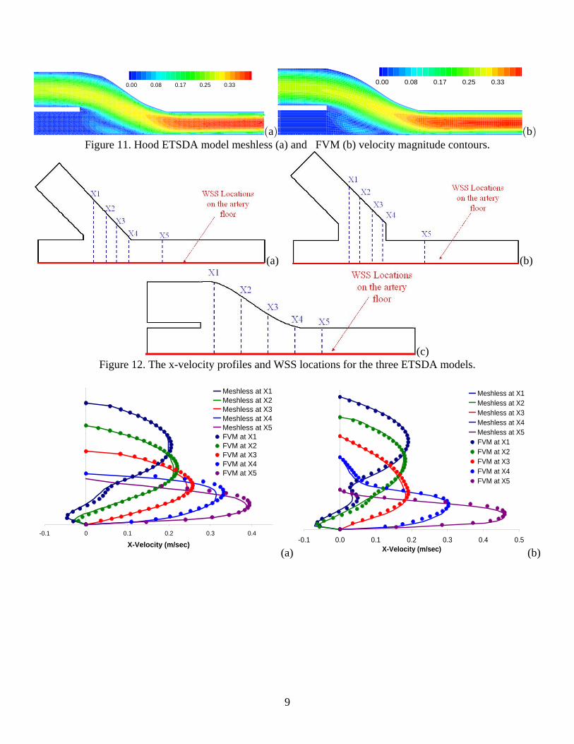
The localized meshless and the FVM results are compared qualitatively in terms of velocity magnitude, x-velocity profiles and the WSS computed on the floor of the host artery. The velocity magnitude comparison isprovided in Figures 9, 10, and 11 for the conventional, Miller Cuff, and hood ETSDA models respectively. Thevelocity magnitude contours of the three ETSDA models demonstrate a very good qualitative agreementbetween the values predicted by the FVM and the localized meshless solvers. Particularly, the meshless methodis capable of capturing the flow recirculation at the floor of the host artery consistently with the FVM.Moreover, the flow acceleration as it emerges from the graft to the artery as predicted by the meshless solveragrees well with that predicted by the FVM solver.

8

To validate the accuracy of the meshless method quantitatively, we plot the meshless and FVM x-velocityprofiles at five vertical sections (X1, X2, X3, X4, and X5) across the anastomoses of the three given ETSDAmodels. The locations of the velocity profiles for the three given ETSDA models are revealed in Figure 12.athrough Figure 12.c. The velocity profiles results are shown for the conventional ETSDA model, Miller CuffETSDA model, and the hood ETSDA model in Figures 13.a, 13.b, and 13.c respectively. Although minordiscrepancies are evident, the velocity profiles indicate a high level of quantitative agreement between themeshless method and the FVM.

Figure 7. The meshless point distribution.

Figure 8. The FVM meshes.

0.00 0.03 0.07 0.10 0.13 0.17 0.20 0.23 0.27 0.30 0.33 0.37 0.40 0.00 0.03 0.07 0.10 0.13 0.17 0.20 0.23 0.27 0.30 0.33 0.37 0.40

baFigure 9. Conventional ETSDA model meshless (a) and FVM (b) velocity magnitude contours.

0.00 0.06 0.12 0.17 0.23 0.29 0.35 0.40 0.46 0.00 0.06 0.12 0.17 0.23 0.29 0.35 0.40 0.46

a bFigure 10. Miller Cuff ETSDA model meshless (a) and FVM (b) velocity magnitude contours.

9

0.00 0.08 0.17 0.25 0.33 0.00 0.08 0.17 0.25 0.33

a bFigure 11. Hood ETSDA model meshless (a) and FVM (b) velocity magnitude contours.

(a) (b)

(c)Figure 12. The x-velocity profiles and WSS locations for the three ETSDA models.

-0.1 0 0.1 0.2 0.3 0.4

X-Velocity (m/sec)

Meshless at X1Meshless at X2Meshless at X3Meshless at X4Meshless at X5FVM at X1FVM at X2FVM at X3FVM at X4FVM at X5

-0.1 0.0 0.1 0.2 0.3 0.4 0.5X-Velocity (m/sec)


(a) (b)

10

-0.1 0.0 0.1 0.2 0.3 0.4X-Velocity (m/sec)


(c) Figure 13. The x-velocity profiles for the ETSDA models.

Due to the adverse effects of its spatial and temporal gradients on the endothelium, we benchmark themeshless results of the WSS at the floor of the host artery with the WSS results generated by the FVM solverfor all the ETSDA models. The development of the IH on the host artery floor is thought to be purely caused byfluid mechanics factors, unlike the situation at the suture line where injury and graft-artery compliancemismatch play a main role []. The two-dimensional WSS magnitude is expressed such as:

[WW œ .½ ½>p 10

where > B Cp

is the traction vector and its and components are:

> œ # 8 B`? `? `@

`B `C `BB B CŒ 11

> œ 8 # 8`? `@ `@

`C `B `CC B CŒ 12

where and are respectively the - and -components of the outward drawn unit normal vector at the8 8 B CB C

boundary. The meshless and FVM plots of the WSS for the conventional, Miller Cuff, and hood ETSDAmodels on their host artery floors (marked by the red line in each of Figures 12. 12. 12. ) are presenteda, b, and cin Figures 14.a, 14.b, and 14.c respectively. 14The WSS results in Figure reflect an acceptable agreementbetween the meshless method and the FVM. The minor discrepancies in the WSS between the two methods isdirectly attributed to the discrepancies found in the x-velocity profiles already pointed out in Figure . Should13the x-velocity profiles perfectly match, there will be no differences in the WSS as extracted from both methods.

11

0.0

0.5

1.0

1.5

2.0

2.5

3.0

3.5

4.0

4.5

0.050 0.060 0.070 0.080 0.090Artery Axial Distance (m)

WSS

(N/m

2)

Meshless WSSFVM WSS

0.0

1.0

2.0

3.0

4.0

5.0

6.0

7.0


WSS

(N/m

2)

Meshless WSSFVM WSS

(a) (b)

0

0.5

1

1.5

2

2.5

3

3.5


WSS

(N/m

2)

Meshless WSS

FVM WSS

(c)Figure 14. Meshless and FVM WSS plots at the artery floor for all the ETSDA models.

3. The Genetic-Algorithm-Based ETSDA Shape Optimization

3.1. The Operation of Genetic Algorithms

Genetic algorithms (GA) are evolutionary optimization techniques, that is they utilize ideas and takeinspirations from the natural evolution of living systems. Evolutionary optimization are well suited tooptimization of systems that exhibit high non-linear behaviors and they are characterized by several featuresthat distinguish them from other optimization algorithms. First, they work with an assembly of differentsolutions, this is called the population of individuals, instead of only working with a single individualrepresenting one solution. Second, there is communication and information exchange among individuals in thepopulation. Such communications and information exchange are the result of the individuals selection and/orrecombination at each generation of the evolution. Third, all the evolutionary optimization algorithms convergeto a final generation mostly consisting of "elite individuals" that represent the best solutions.

A comprehensive review and insight on the GA can be found in Goldberg [35]. For a shape optimizationapplication, the GA process begins by randomly setting an initial population of possible individuals, where eachindividual represents a random geometry defined by a set of design variables. This population maintains thesame number of individuals as it evolves throughout successive generations. Each individual is referred to as a‘chromosome’ containing the binary representation of its design variables referred to as ‘genes’ of thechromosome to which genetic operators are applied. Figure 15 illustrates the genetic encoding of a givenindividual or chromosome. Each design variable is bounded with a minimum and a maximum value, forming asearch range for the optimal solutions are sought. The genetic representation of the problem will be crucial to

12

the success of the GA. The fitness, , of each individual in the population treated by the GA is evaluatedF1through an objective function, .ZGA

GA relies on an iterative approach and at each iteration, the processes of selection, cross-over, andA typicalmutation operators are used to alter the individuals optimization parameters such that Z is minimized [40]. AGAselection operator is first applied to the population in order to determine and select the individuals that aregoing to pass information in a mating process with the rest of the individuals in the population. The probabilityof being a selected individual is calculated as the ratio between the value of the fitness function of eachindividual and the sum of all objectives function values. A weighted roulette wheel is generated, where eachmember of the current population is assigned a portion of the wheel in proportion to its probability of selection.The wheel is spun as many times as there are individuals in the population leading to the survival of the bestchromosomes and the death of the worst ones. The selection process could be elitist whereby a number of theselected individuals are transferred directly to the new generation without undergoing the cross-over andmutation processes [36,37] The elitist selection approach has been proven to speed-up the GA convergence by. preventing the loss of the identified good solutions [38]. The selection approach employed in this paper is notformally elitist as only the best selected individual is directly transferred to the new generation. For the rest ofthe selected individuals which have not been directly transferred to the new generation, the cross-over or matingprocess starts the genetic information contained to be combined and henceto allow of those individualsgenerate offsprings. randomly affects the informationThe mutation is the final operator that is applied toobtained by the mating of individuals for further genetic improvement. Two types of mutations are commonlyutilized in GA's [35,39]: the creep mutation and the jump mutation. With regards to creep mutation, a creepprobability is assigned to every bit of each individual/chromosome in the population; if the mutation iseffective, the bit will be switched from 0 to 1 or vice-versa. This process is implemented by generating arandom number within the range (0...1) for each bit within the chromosome. If the generated number is smallerthan the mutation probability the bit is mutated. Concerning the jump mutation, a jump probability is applied toevery chromosome/individual in the population. If the jump mutation is effective, all bits within thechromosome/individual are switched from 0 to 1 and vice-versa. Djurisic [36] introduced an adaptive mutationtechnique by which each gene within of a newly-born individual is mutated based on that gene average valuefor all the individuals within the given population. Following selection, crossover and mutation the newpopulation is ready for its next evolution until the convergence criteria "fitness" is reached. In summary, thegenetic algorithms can be applied as follows:

1. Generate the initial population P(0) at random and set =0 i2. REPEAT a. Evaluate the Fitness of each individual in P( ) i b. Select Parents from P( ) based on their fitness as follows:i Given the fitness of individuals as 8 F ,F ,...,F " 2 nÞ Then, select individual with3 probability expressed in equation 13,

: œ Ð Ñ33

4œ"

8

3

F

F13

This is often called roulette wheel selection

13

d. Apply CROSSOVER to selected parents. e. Apply mutation to crossed-over new individuals. f. Replace parents by the offspring to produce generation P( +1) i3. UNTIL the desired criterion is satisfied.

Figure 15. Example of an individual characterized by four genes encoded in a chromosome.

3.2. The ETSDA Shape Optimization Objective Function

Having already discussed the damaging impact of the SWSSG on the endothelium, an ideal objective to beachieved by shape optimization of the ETSDA would be to arrive at a geometry that minimizes the high valuesof this hemodynamics wall parameters on the floor of the host artery. The two-dimensional SWSSG magnitudeis expressed as:

l lÍÍÍÍÍÌ

Ô × Ô ×Ö Ù Ö ÙÕ Ø Õ ØŒ ŒŒ ŒW[WWK œ # B C # B C

` ? ` ? ` @ > ` ? ` ? ` @

`B `B`C `B `B`C `C `B`C

># # # # # #

# # #8 8 8 8B

# #

C

½ ½ ½ ½> >p p 14

The SWSSG is essentially a tensor, and the expression of its magnitude in Equation 14 only considers thetensor entries that tangentially affect the endothelial cells. Kleinstreuer at al. [41] discussed the formulation ofthe current SWSSG magnitude expression. Examining Figures 9, 10, and 11, one can predict high SWSSGvalues at the floor occurring near the disturbed flow area where there is a flow recirculation and a stagnationpoint resulting from the flow impingementÞOn the other hand, the SWSSG values are expected to drop in thedead zone area at the host artery proximal side near the blockage and towards the outlet at the host artery distalside where the flow tends to regain its laminar parabolic shape. Plots of the SWSSG values for typical andoptimal shapes of the conventional, Miller cuff, and hood ETSDA models are shown respectively in Figures 19,22, and 26; note the spiking SWSSG values at the artery floor section across from the suture line (flowimpingement site) as well as the SWSSG small values near the designated outlet at x = 0.009 (m) (recoveredparabolic flow site). Thus, we would like to formulate a shape optimization objective function that representsthe high values of the SWSSG at the host artery floor section where IH tends to develop. The objective functioncan be selected as the L norm of the SWSSG magnitude at every boundary node on the host artery floor#

section that is opposite to the suture line; we call this section as the ‘floor optimization section’ Thus, theobjective function, , can be expressed as:F

14

J œ"

R

ÍÍÍÌ l lFJ +<>/<C3œ"

RFJ W[WWK

(1/D )15

where, is the number of boundary points on the floor optimization section. The magnitude values ofRFJ

SWSSG are controlled by the design variables of the ETSDA. After all, the anastomotic geometry plays a bigrole in modifying the fluid mechanics parameters at the boundary walls. Hence, implicitly depends on theJETSDA design variables that control the magnitudes of SWSSG.

3.3. The ETSDA Shape Optimization Objective Function

The current shape optimization is based on Information Passage Loop (IPL) that is comprised of threeandifferent computational objects: (1) the automated preprocessor, (2) the meshless solver, and (3) the shapeoptimization genetic algorithm (SOGA). The goal of establishing the IPL is to provide a tool that can iterativelysearch for the optimal ETSDA shape within a design variable search range. This search should be autonomousfrom beginning to end, without any user intervention, see Figure 16, for a simple flowchart.

Figure 16. The IPL flowchart.

This GA-based optimization starts by setting an initial population of individuals, each representing anETSDA geometry. Each individual or geometry possesses genes that represent its design variables. The initialpopulation of ETSDA geometries undergoes an evolution throughout several generations following an iterativeprocess, where each generation is considered as an iteration. At each iteration of this evolutionary process thefollowing three tasks are executed within the IPL. First, the automated preprocessor reads the geometry of eachETSDA geometry and performs a point distribution therein. Second, all the ETSDA preprocessed geometriesare exported to the meshless solver where the flow field is solved within each model. Once the flow field issolved, the SWSSG magnitudes on the host artery floor are post-processed and the fitness function is evaluatedfor each individual. It should be noted that the fitness function value for each individual is simply computed asthe inverse of the objective function value. Third, all the ETSDA fitness function values are sent to the SOGAwhere the selection, mating and mutation processes occur leading to a new modified set of design variables.This new set of design variables is passed to the automated preprocessor to again start a new iteration. It isimportant to mention at this point that without having an automated preprocessor, it would not be possible to

15

establish the IPL in an autonomous fashion. In other words, without the automated preprocessor, the user willhave to intervene at every iteration to interactively preprocess the geometries which design variables have beenmodified by the SOGA. This intervention will make the current optimization tool highly inefficient.

The shape optimizations of the conventional, Miller Cuff, and hood ETSDA models depend on a set ofdesign variables that control their geometries. Those design variables are limited by a search range over whichthe optimal shape of the ETSDA has be located. The search ranges for the three ETSDA models considered inthis paper are chosen arbitrarily. In the event of a patient-based peripheral bypass surgery, the search rangesshould be set up to the discretion of the vascular surgeon, who is the principal person to estimate the surgicalfeasibility. For all the three ETSDA models, a population with a fixed size of 34 is chosen. The jump and creepmutation probabilities for the current GA-based optimization are taken as 0.02 and 0.2 respectively. Also, thehost artery diameter is taken as constant and equal to 4 mm for all the three anastomotic models and the inletvolumetric flow rate is taken as 480 ml/min (corresponding to a graft-diameter-based Re number of 450).

For each of the three ETSDAs shape optimizations there is one reference case and four supportive cases.The purpose of the reference case is to establish a basic convergence history of the objective function and use itas a basis of comparison. The four supportive cases are run to support the consistency argument of thealgorithm. All the reference and supportive cases follow the same composed objective function and they operatein the same search ranges. The only difference between each of these cases is the initial population which theevolutionary optimization algorithm starts off. The convergence consistency should give more confidence in theidentified optimal variables. There is no preset convergence criterion, rather each optimization run is allowed75 generations. While this might not lead to the absolute optimal solution, a significant drop in the objectivefunction should be noted through the 75 generations. A signigficant limitation to increasing the number ofgenerations is the CPU time consumed by the numerical solution of the Navier-Stokes equation; this numericalsolution is inevitable as there is no analytical or empirical approaches to assess the SWSSG values in anintricate geometry such the one of the ETSDA.

3.3.1. The Conventional ETSDA Model Shape Optimization Results

The set of design variables for the conventional ETSDA model consists of two parameters: the anastomoticangle, , and the graft caliber, D . The search range for is limited between 30° and 60°, whereas the" "1<+0>

search range for D is limited between 4 mm and 6 mm. The generatrix of the Direct ETSDA model is1<+0>

shown in Figure 17. The predicted optimization outcomes and statistics at the 75th generation for theconventional ETSDA optimization variables are reported in Table 1. The convergence history of the referenceand supportive objective functions for the conventional ETSDA shape optimization are displayed in Figure 18.In order to illustrate the gain achieved by the conventional ETSDA shape optimization, we plot in Figure 19 theSWSSG values on the floor optimization sections of both the current optimized shape and a selected standardshape considered for optimization. We choose the standard shape to be the one shown in Figure 6.a ( =45° and"D =6 mm). Although both SWSSG plots in Figure exhibit similar trends, notice that the red curve1<+0>

(corresponding to the standard shape) has been lowered to the level of the blue curve (corresponding to theoptimized shape) thanks to the shape optimization process.

A conclusion can be drawn from the conventional ETSDA optimization results that the optimized shapetends to take the lower limit of and the upper limit of D . To reinforce this conclusion, a supplemental" 1<+0>

optimization solution was carried out with wider variable search ranges whereby D and were allowed to1<+0> "vary respectively within the following search ranges [3-7 mm], [20-70 deg]. The resolved optimal values were

16

identified as 6.937 mm for D and 20 deg for . Therefore, it can be concluded that a conventional ETSDA1<+0> "model should have the lowest possible angle and the highest graft diameter for a minimal SWSSG at the hostartery floor.

2.5

2.7

2.9

3.1

3.3

3.5

1 16 31 46 61

Number of Generations

Obj

ectiv

e Fu

nctio

n

Reference CaseCase 1Case 2Case 3Case 4

Figure 17. The conventional ETSDA model generatrix. Figure 18. The convergence history for all the conventional ETSDA model cases.

Table 1. Shape optimization results and statistics for the conventional ETSDA model.Graft Diameter (mm) Angle (deg)

Reference Case 5.96863 30.71Case 1 5.96500 31.57Case 2 5.73100 32.31Case 3 5.90000 31.78Case 4 5.75700 30.67

Mean Value 5.86433 31.41Standard Deviation 0.11356 0.71

0.0

300.0

600.0

900.0

1200.0

1500.0

1800.0


SWSS

G (N

/m3)

Optimized Conventional ETSDA

Standard Conventional ETSDA

Figure 19. SWSSG plots for the standard and optimized conventional ETSDA models.

3.3.2. The Miller Cuff ETSDA Model Shape Optimization Results

17

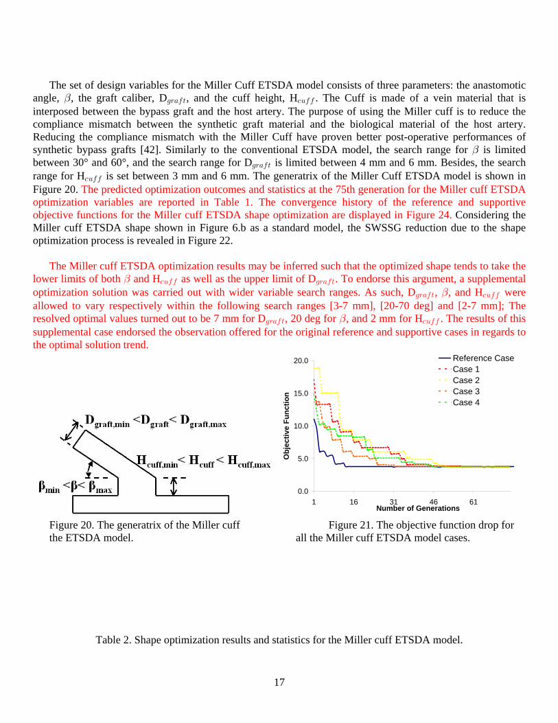
The set of design variables for the Miller Cuff ETSDA model consists of three parameters: the anastomoticangle, , the graft caliber, D , and the cuff height, H . The Cuff is made of a vein material that is" 1<+0> -?00

interposed between the bypass graft and the host artery. The purpose of using the Miller cuff is to reduce thecompliance mismatch between the synthetic graft material and the biological material of the host artery.Reducing the compliance mismatch with the Miller Cuff have proven better post-operative performances ofsynthetic bypass grafts [42]. Similarly to the conventional ETSDA model, the search range for is limited"between 30° and 60°, and the search range for D is limited between 4 mm and 6 mm. Besides, the search1<+0>

range for H is set between 3 mm and 6 mm. The generatrix of the Miller Cuff ETSDA model is shown in-?00

Figure 20. The predicted optimization outcomes and statistics at the 75th generation for the Miller cuff ETSDAoptimization variables are reported in Table 1. The convergence history of the reference and supportiveobjective functions for the Miller cuff ETSDA shape optimization are displayed in Figure 24. Considering theMiller cuff ETSDA shape shown in Figure 6.b as a standard model, the SWSSG reduction due to the shapeoptimization process is revealed in Figure 22.

The Miller cuff ETSDA optimization results may be inferred such that the optimized shape tends to take thelower limits of both and H as well as the upper limit of D . To endorse this argument, a supplemental" -?00 1<+0>

optimization solution was carried out with wider variable search ranges. As such, D , , and H were1<+0> -?00"allowed to vary respectively within the following search ranges [3-7 mm], [20-70 deg] and [2-7 mm]; Theresolved optimal values turned out to be 7 mm for D , 20 deg for , and 2 mm for H . The results of this1<+0> -?00"supplemental case endorsed the observation offered for the original reference and supportive cases in regards tothe optimal solution trend.

0.0

5.0

10.0

15.0

20.0

1 16 31 46 61Number of Generations

Obj

ectiv

e Fu

nctio

n


Figure 20. The generatrix of the Miller cuff Figure 21. The objective function drop for the ETSDA model. all the Miller cuff ETSDA model cases.

Table 2. Shape optimization results and statistics for the Miller cuff ETSDA model.

18

Graft Diameter (mm) Angle (deg) Cuff Height (mm)Reference Case 5.90588 32.94120 3.05882

Case 1 5.96100 31.82000 3.50000Case 2 5.71200 31.69000 3.26700Case 3 5.73900 30.70000 3.38100Case 4 5.73900 32.71000 3.17000

Mean Value 5.81138 31.97224 3.27536Standard Deviation 0.11366 0.89507 0.17298

0.0

500.0

1000.0

1500.0

2000.0

2500.0

3000.0

3500.0


SWSS

G (N

/m3)

Optimized Miller ETSDA

Standard Miller ETSDA

Figure 22. SWSSG plots for the standard and optimized Miller cuff ETSDA models.

3.3.3. The Hood ETSDA Model Shape Optimization Results

For the hood ETSDA model, we adapt a fixed diameter of 6 mm for the graft. Given a cut length of 15 mm,the anastomosis shape variability only depends on the cubic spline defining the hood shape. The two endcontrol points of the spline the other two control points c and c are kept fixed, whereas c and c are allowedg a 1 2to move within limited specified two-dimensional ranges. The ranges of motion for c and c are specified1 2within a two-dimensional coordinate system representing the ETSDA hood model generatrix that is shown inFigure 23. The predicted optimized coordinates and statistics at the 75th generation for c and c are reported in1 2Table 1. The convergence history of the reference and supportive objective functions for the hood ETSDAshape optimization are displayed in Figure 24. Additionally, the optimized shapes of the reference andsupportive cases are revealed in Figure 25; the prominent similarity of those shapes illustrates the convergenceconsistency of all the considered hood ETSDA shape optimization cases. The hood ETSDA model shown inFigure 6.c is picked as a non-optimal shape; the coordinates of the moving control points of this model are:x1=3.75, y1=6.12, x2=11.25, and y2=1.36. Plots of the SWSSG on the host artery floor of both the standard andthe optimized hood ETSDA models are shown in Figure 26. The narrow modification from the standard hoodETSDA shape to the optimized hood ETSDA shape justifies the slight drop in the SWSSG values in Figure 26.

19

1.5

2.0

2.5

3.0

3.5

1 21 41 61Number of Generations

Obj

ectiv

e Fu

nctio

n


Figure 23. The generatrix of the hood ETSDA Figure 24. The objective function minimization for model. all the hood ETSDA cases.

Table 3. Shape optimization results and statistics for the hood ETSDA model.x2 (mm) y2 (mm) x1 (mm) y1 (mm)

Reference Case 12.378 1.857 4.027 6.717Case 1 12.538 1.782 3.951 6.731Case 2 12.434 1.936 4.065 6.710Case 3 12.326 1.881 3.950 6.718Case 4 12.416 1.810 3.965 6.723

Mean Value 12.419 1.853 3.992 6.720Standard Deviation 0.07867416 0.06040085 0.05167812 0.008107732

1.36

3.36

5.36

3 6 9 12x (mm)

y (m

m)

Reference Case Case 1Case 2Case 3Case 4

0.0

300.0

600.0

900.0

1200.0

1500.0


SWSS

G (N

/m3)

Optimized Hood ETSDA

Standard Hood ETSDA

Figure 25. The optimized hood shapes for the reference Figure 26. SWSSG plots for the standardand the four supportive cases. .and the optimized reference Hood ETSDA models

4. Conclusion

The shape improvement of the bypass grafts ETSDA can lower morbidity and reduce medical costs forpatients suffering from peripheral vascular diseases. Therefore, a serious effort should be taken to address this

20

shape optimization subject. In this paper, shape optimizations for the conventional, Miller Cuff, and hoodETSDA models were performed to inhibit IH growth on the host artery floor. The focus on the floor of the hostartery is because IH thereat is mainly affected by hemodynamics forces. The present shape optimizations arebased on a genetic algorithm and their objective is to reduce the SWSSG on the floor of the host artery. Thecurrent optimization approach has proven to be successful in terms of building the communication betweenthree different computational objects: the automated pre-processor, the meshless CFD solver and the SOGA. Atthe time being, we cannot extend recommendations to vascular surgeons on how to design their arterialanastomoses; however future recommendations will be potentially made once the blood pulsatility and thegraft-to-artery compliance mismatch are accounted for in the optimization process. The study reported hereinestablishes the methodology as a viable means of achieving optimal ETSDA shapes. We leave the aspects ofpulsatile and non-Newtonian flow to a follow-up study and note additionally that we are extending our work tothree-dimensions to bring in perspectives of three dimensional effects such as the secondary flows, for instancethe Dean vortices that are absent in the current study.

5. References

[1] Z. El Zahab, E. Divo, A. Kassab, "Shape Optimization of Bypass Grafts End-to-side Distal Anastomosis",in Miami, FL, USA, (2007).Inverse Problems, Design and Optimization Symposium,

[2] E. Mitteff, E. Divo, and A. Kassab, "Automated Point Distribution and Parallel Segmentation forMeshless Methods", in B. Gamez, D. Ojeda, G. Larrazabal., and M. Cerrolaza, editors, Proceedings ofCIMENICS 2006, 8th International Congress of Numerical Methods in Engineering and Applied Sciences,Sociedad Venezuelana de Methodos Numericos En Engineria, Valencia, Venezuela, (2006) 93-100.

[3] T. Belytscho, Y. Y. Lu, and L. Gu, "Element-free Galerkin methods", International Journal of NumericalMethods, 37, (1994) 229-256.

[4] S. N. Atluri and S. Shen, Tech. Science Press, Encino, CA, USA, 2002.The Meshless Method.

[5] S. N. Atluri and T. Zhu, "A New Meshless Local Petrov-Galerkin (MLPG) Approach in ComputationalMechanics", 117-127.Computational Mechanics, , (1998)22

[6] G. R. Liu, CRC Press, Boca Raton, FL, USA, 2003.Mesh Free Methods.

[7] E. J. Kansa, "Multiquadrics- a scattered data approximation scheme with applications to computationalfluid dynamics I- surface approximations and partial derivative estimates", Comp. Math. Appl., ,19 (1990)127-145.

[8] E. J. Kansa, "Multiquadrics- a scattered data approximation scheme with applications to computationalfluid dynamics II - solutions to parabolic, hyperbolic and elliptic partial differential equations", Comp.Math. Appl ., (1990)19 147-161.

[9] E. J. Kansa and Y. C. Hon, "Circumventing the Ill-Conditioning Problem with Multiquadric Radial BasisFunctions: Applications to Elliptic Partial Differential Equations", 123-137.Comp. Math. Appl , ,. (2000)39

21

[10] E. Divo and A. Kassab, "A Meshless Method for Conjugate Heat transfer," , ,Engineering Analysis 29(2005) 136-149.

[11] B. Sarler, T. Tran-Cong, and C. S. Chen, "Mesh Free Direct and Indirect Local Radial Basis Function Collocation Formulations for Transport Phenomena", in Boundary Elements XVII, A. Kassab, C. A.Brebbia, and E. Divo, editors, WIT Press, Southampton, UK, (2005) 417-428.

[12] E. Divo and A. Kassab "Modeling of Convective and Conjugate Heat Transfer by a Third Order LocalizedRBF Meshless Collocation Method," in ASME International Mechanical Engineering Congress and RD & D Expo, Orlando, FL, USA, (2005).

[13] Z. El Zahab, E. Divo, and A. Kassab, "Parallel Domain Decomposition Meshless Modeling of DiluteChemical Species Transport", in The 2005 Technical Meeting of the Eastern States Section of theCombustion Institute, Orlando, FL, USA, (2005).

[14] E. Divo and A. Kassab, "Efficient Localized Meshless Modeling of Natural Convective Viscous Flows",AIAA Paper AIAA-2006-3089.

[15] E. Divo and A. Kassab, "Iterative Domain Decomposition Meshless Method Modeling of IncompressibleFlows and Conjugate Heat Transfer", , (2006) 465-478.Engineering Analysis, 30

[16] E. Divo and A. Kassab, "An Efficient Localized RBF Meshless Method for Fluid Flow and ConjugateHeat Transfer", , (2007) 124-136.ASME Journal of Heat Transfer, 129

[17] Z. Two-dimensional Meshless Numerical Modeling of theEl Zahab, E. Divo, A. Kassab, and E Mitteff, "Blood Flow within Arterial End-to-side Distal Anastomoses", in ASME International Mechanical Engineering Congress and RD & D Expo, Chicago, IL, USA, (2006).

[ ] 18 F. J. Veith, , S. K. Gupta, E. Ascer, S. White-Flores, R. H. Samson, L. A. Scher, J. B. Towne, V. M.Bernhard, P. Bonier, W. R. Flinn, P. Astelford, J. S. T. Yao, and J. J. Bergan, "Six-year ProspectiveMulticenter Randomized Comparison of Autologous Saphenous Vein and ExpandedPolytetrafluoroethylene Grafts in Infrainguinal Arterial Reconstructions", , Journal of Vascular Surgery 3(1986) 104-114.

[19] V. S. Sottiurai, J. S. T. Yao, R. C. Batson, S. L. Sue, R. Jone, and Y. A. Nakamura, "Distal AnastomoticIntimal Hyperplasia: Histopathologic Character and Biogenesis", Annals of Vascular Surgery, 3 (1989)26-33.

[20] H. S. Bassiouny, S. White, S. Glagov, E. Choi, D. P. Giddens, and C. K. Zarins, "Anastomotic IntimalHyperplasia: Mechanical Injury or Flow Induced", 708-716. , (1992)Journal of Vascular Surgery 15

[21] W. Trubel, H. Schima, M. Czerny, K. Perktold, M. G. Schimek, and P. Poltrerauer, "ExperimentalComparison of Four Methods of end-to-side Anastomosis with Expanded Polytetrafluoroethylene", BritishJournal of Surgery, (2004) 91 159-167.

22

[22] M. S. Lemson, J. H. Tordoir, M. J. Daemen, and P. J. Kitslaar, "Intimal Hyperplasia in Vascular Grafts",European Journal of Vascular and Endovascular Surgery, (2000) 336-350.19

[23] T. R. Kohler, T. R. Kirkman, L. W. Kraiss, B. K. Zierler, and A. W. Clowes, "Increased Blood FlowInhibits Neointimlal Hyperplasia in Endothelialized Vascular Grafts", , Circulation Research 69 (1991)1557-1565.

[24] V. S. Sottiurai, "Distal Anastomotic Intimal Hyperplasia: Histocytromorphology, Pathophysiology,Etiology, and Prevention", International Journal of Angiology, , (1999) 1-10.8

[25] Y. Trady, N. Resnick, T. Nagel, M. A. Gimbrone Jr., and C. F. Dewey Jr., "Shear Stress GradientsRemodel Endothelial Monolayers in Vitro via a Cell Proliferation-Migration-Loss Cycle",Arteriosclerosis, Thrombosis, and Vascular Biology, ,17 (1997) 3102-3106.

[26] P. P. Hsu, L. Song, Y. Li, S. Usami, A. Ratcliffe, X. Wang, and S. Chien, "Effects of Flow Patterns onEndothelial Cells Migration into a Zone of Mechanical Denudation", Biochemical and BiophysicalResearch Communications, (2001) 751-759.285

[27] M. Ojha, "Spatial and Temporal Variations of Wall Shear Stress within and End-to-Side ArterialAnastomoses Model," 1377-1388.Journal of Biomechanics, 26 (1993)

[28] M. Lei, D. P. Giddens, S. A. Jones, F. Loth, and H. Bassiouny, "Pulsatile Flow in an End-to-Side VascularGraft Model: Comparison of Computations with Experimental Data", Journal of BiomechanicalEngineering, 123 (2001) 80-87.

[29] M. Lei, J. P. Archie, and C. Kleinstreuer, "Computational Design of a Bypass Graft that minimizes WallShear Stress Gradients in the Region of the Distal Anastomosis", Journal of Vascular Surgery, 25 (1997)637-646.

[30] R. K. Fisher, T. V. How, T. Carpenter, J. A. Brennan, and P. L. Harris, "Optimising Miller CuffDimensions. The Influence of Geometry on Anastomotic Flow Patterns", European Journal of Vascularand Endovascular Surgery, 251-260.21 (2001)

[31] T. O'Brien, M. Walsh, and T. McGloughlin, "On Reducing Abnormal Hemodynamics in the Femoral End-to-Side Anastomosis: The Influence of Mechanical Factors," Annals of Biomedical Engineering, 33(2005) 310-322.

[32] G. Rozza,"On optimization, control and shape design for an arterial bypass", International Journal forNumerical Methods in Fluids, Bill Morton Prize Paper, , (2005) 1411-1419.47

[33] Z. El Zahab, E. Divo, A. Kassab, "Shape Optimization of Bypass Grafts End-to-side Distal Anastomosis",in Miami, FL, USA, (2007).Inverse Problems, Design and Optimization Symposium,

[34] E. Mitteff, E. Divo, and A. Kassab, "Automated Point Distribution and Parallel Segmentation forMeshless Methods", in B. Gamez, D. Ojeda, G. Larrazabal., and M. Cerrolaza, editors, Proceedings of

23

CIMENICS 2006, 8th International Congress of Numerical Methods in Engineering and Applied Sciences,Sociedad Venezuelana de Methodos Numericos En Engineria, Valencia, Venezuela, (2006) 93-100.

[35] D. E. Goldberg, Addison-Wesley,Genetic Algorithms in Search, Optimization and Machine Learning.Reading, MA, USA, 1989.

[36] A. B. Djuricic, "Elite Genetic Algorithms with Adaptive Mutations for Solving Continuous OptimizationProblems - Application to Modeling of the Optical Constants of Solids," , ,Optics Communications 151(1998), 147-159.

[37] K. Deb, A. Pratrep, S. Agarwal, and T. Meyarivan, " A Fast and Elitist Multiobjective Genetic Algorithm:NSGA II," , (2002), 182-197.IEEE Transactions on Evolutionary Computation 6,

[38] E. Zitzler, K. Deb, and L. Thiele, "Comparison of Multiobjective Evolutionary Algorithms," EvolutionaryComputation, , (2000), 173-195.8

[39] E. Divo, A. J. Kassab, and F. Rodriguez, "Characterization of Space Dependent Thermal Conductivitywith a BEM-Based Genetic Algorithm," , , (2000) pp.Numerical Heat Transfer, Part A: applications 37845-877.

[40] E. Divo, A. J. Kassab Shape optimization of acoustic scattering bodies," , and M. S. Ingber, " EngineeringAnalysis with Boundary Elements, ,27 (2003), 695-704.

[41] C. Kleinstreuer, S. Hyun, J. R. Buchanan Jr., P. W. Longest, J. P. Archie Jr., and G. A. Truskey,"Hemodynamics Parameters and Early Intimal Thickening in Branching Blood Vessels", Critical Reviewsin Biomedical Engineering, 29, (2001) 1-64.

[42] M. Raptis and J. H. Miller, "Influence of a Vein Cuff on Ploytetrafluoroethylene Grafts for PrimaryFemoropopliteal Bypass", , , (1995) 487-491.British Journal of Surgery 82

a meshless cfd approach for evolutionary shape...

Documents