A Lagrangian Meshless Finite Element Method applied to Fluid-Structure Interaction Problems

S.R. Idelsohn(1,2), E. Oñate(2), F. Del Pin(1)

. International Center for Computational Methods in Engineering (CIMEC)

Universidad Nacional del Litoral and CONICET, Santa Fe, Argentina e–mail: sergio@ceride.gov.ar

International Center for Numerical Methods in Engineering (CIMNE)

Universidad Politécnica de Cataluña, Barcelona, Spain e–mail: onate@cimne.upc.es

Key words: Fluid-Structure interaction, Particle methods, Lagrange formulations, Incompressible Fluid Flows, Meshless Methods, Finite Element Method. Abstract A method is presented for the solution of the incompressible fluid flow equations using a lagrangian formulation. The interpolation functions are those used in the Meshless Finite Element Method (MFEM) and the time integration is introduced in a semi-implicit way by a fractional step method. Classical stabilization terms used in the momentum equations are unnecessary due to the lack of convective terms in the lagrangian formulation. Furthermore, the lagrangian formulation simplifies the connections with fixed or moving solid structures, thus providing a very easy way to solve fluid-structure interaction problems. 1 Introduction Over the last twenty years, computer simulation of incompressible fluid flow has been based on the Eulerian formulation of the fluid mechanics equations. However, it is still difficult to analyze problems in which the shape of the interface changes continuously or in fluid-structure interactions with free-surfaces where complicated contact problems are involved. More recently, Particle Methods in which each fluid particle is followed in a lagrangian manner have been used [1-4]. The first ideas on this approach were proposed by Monaghan [1] for the treatment of astrophysical hydrodynamic problems with the so called Smooth Particle Hydrodynamics Method (SPH). This method was later generalized to fluid mechanic problems [2-4]. Kernel approximations are used in the SPH method to interpolate the unknowns. On the other hand, a family of methods called Meshless Methods have been developed both for structural [5,6] and fluid mechanics problems [8-10]. All these methods use the idea of a polynomial interpolant that fits a number of points minimizing the distance between the interpolated function and the value of the unknown point. These ideas were proposed first by Nayroles et al. [7], they were later used in structural mechanics by Belytschko et al. [5]

and in fluid mechanics problems by Oñate et al. [8-10]. In a previous paper [11] the authors presented the numerical solution for the fluid mechanics equations using a lagrangian formulation and a meshless method called the Finite Point Method. Lately, the meshless ideas were generalized to take into account the finite element type approximations in order to obtain the same computing time in mesh generation as in the evaluation of the meshless connectivities [12,13]. This method was called the Meshless Finite Element Method (MFEM) and uses the Extended Delaunay Tessellation [14] to build the mesh in a computing time which is linear with the number of nodal points. In this paper new ideas and results for the solution of a particle method in the field of Fluid-Structure Interaction (FSI) using the Meshless Finite Element Method are presented. A more general formulation is used in which all the classical advantages of the FEM for the evaluation of the unknown functions and derivatives are preserved. Different strategies have been proposed to solve FSI problems. The selection of the most effective approach depends largely on the nature of the problem to be analyzed [15]. Depending on the degree of coupling between the equations for the fluid and the structure, two cases can be distinguished. The first one occurs when there is a strong coupling between the fluid flow and the elastic deformation of the structure [15-17]. The second case occurs when there is a weak interaction between the fluid and the rigid deformation of the structure. In the latter, the solid must undergo large rigid displacements interacting with the fluid. This is the case for instance of sea-keeping in ship hydrodynamics, rotating turbines, mills, and other engines with a moving solid inside a fluid. Both cases of FSI are more easily studied with a lagrangian formulation of the fluid equations, which can be seen as a solid with a small shear coefficient or vice versa. The lagrangian fluid flow equations for the Navier-Stoke problem will be revised in the next section, the Meshless Finite Element Method (MFEM) will be summarized in the Appendix and both techniques will be used to solve some FSI problems for rigid solids. 2 Governing equations The mass and momentum conservation equations can be written in a lagrangian formulations as: Mass conservation:

0=∂

∂+

ixiu

DtD

ρρ (1)

Momentum conservation:

ifijjx

pixDt

iDuρτρ +

∂∂

+∂∂

−= (2)

where ρ is the density iu are the Cartesian components of the velocity field, p the

pressure, ijτ the deviator stress tensor, if the source term (normally the gravity) and DtDφ

represents the total or material time derivative of a function φ .

For Newtonian fluids the stress tensor ijτ may be expressed as a function of the velocity field through the viscosity µ by

)32( ij

l

l

i

j

j

iij x

uxu

xu

δµτ∂∂

−∂

∂+

∂∂

=

(3)

For near incompressible flows (l

k

i

i

xu

xu

∂∂

<<∂∂

) the term :

03

2≈

∂∂

i

i

xuµ (4)

and it may be neglected in eq.(3). Then:

)(i

j

j

iij x

uxu

∂

∂+

∂∂

≈ µτ (5)

In the same way, the term ijjxτ

∂∂ in the momentum equations may be simplified for slow

incompressible flows as:

)()()(

)()())((

j

i

jj

j

ij

i

j

i

j

jj

i

ji

j

j

i

jij

j

xu

xxu

xxu

x

xu

xxu

xxu

xu

xx

∂∂

∂∂

≈∂

∂

∂∂

+∂∂

∂∂

=∂

∂

∂∂

+∂∂

∂∂

=∂

∂+

∂∂

∂∂

=∂∂

µµµ

µµµτ

(6)

Then, the momentum equations can be finally written as:

ij

i

jiiij

ji

i fxu

xp

xf

xp

xDtDu

ρµρτρ +∂∂

∂∂

+∂∂

−≈+∂∂

+∂∂

−= )( (7)

Boundary conditions On the boundaries, the standard boundary conditions for the Navier-Stokes equations are:

niijij p σνντ =− on σΓ (8)

nii uu =ν on nΓ (9)

tii uu =ζ on tΓ (10) where iν and iζ are the components of the normal and tangent vector to the boundary.

3 The time splitting The time integration of equations (7) and (8) presents some difficulties when the fluid is incompressible or nearly incompressible. In this case, explicit time steps cannot be used. Even when using an implicit time integration scheme, incompressibility introduces some wiggles in the pressure solution which must be stabilized. To overcome these difficulties, a fractional step method has been proposed [18] which consists in splitting each time step in 2 steps as follows: Split of the momentum equations

θτ

ρρ+

++

+∂

∂+

∂∂

−=∆

−+−=

∆−

≈ ni

j

ij

i

niii

ni

ni

nii f

xp

xtuuuu

tuu

DtDu

)11(**11

(11)

where nn ttt −=∆ +1 is the time step; ),( nni

ni txuu = ; ),( 111 +++ = nn

ini txuu and *

iu are fictitious variables defined by the split

A) ijn

j

n

ii

nii x

tpx

ttfuu τρ

γρ ∂

∂∆+

∂∂∆

−∆+=* (12)

C) )( 1*1 nn

ii

ni pp

xtuu γρ

−∂∂∆

−= ++ (13)

where γ is parameter equal to cero or one defining a first or second order split, respepctively [18]. Split of the mass conservation equations

i

iini

nnnn

xuuu

ttDtD

∂+−∂

−=∆

−+−=

∆−

≈+++ )( **1**11

ρρρρρρρρ (14)

where *ρ is a fictitious variable defined by the split

i

ini

n

i

in

xuu

t

xu

t

∂−∂

−=∆−

∂∂

−=∆−

++ )( *1*1

**

ρρρ

ρρρ

(15)

(16)

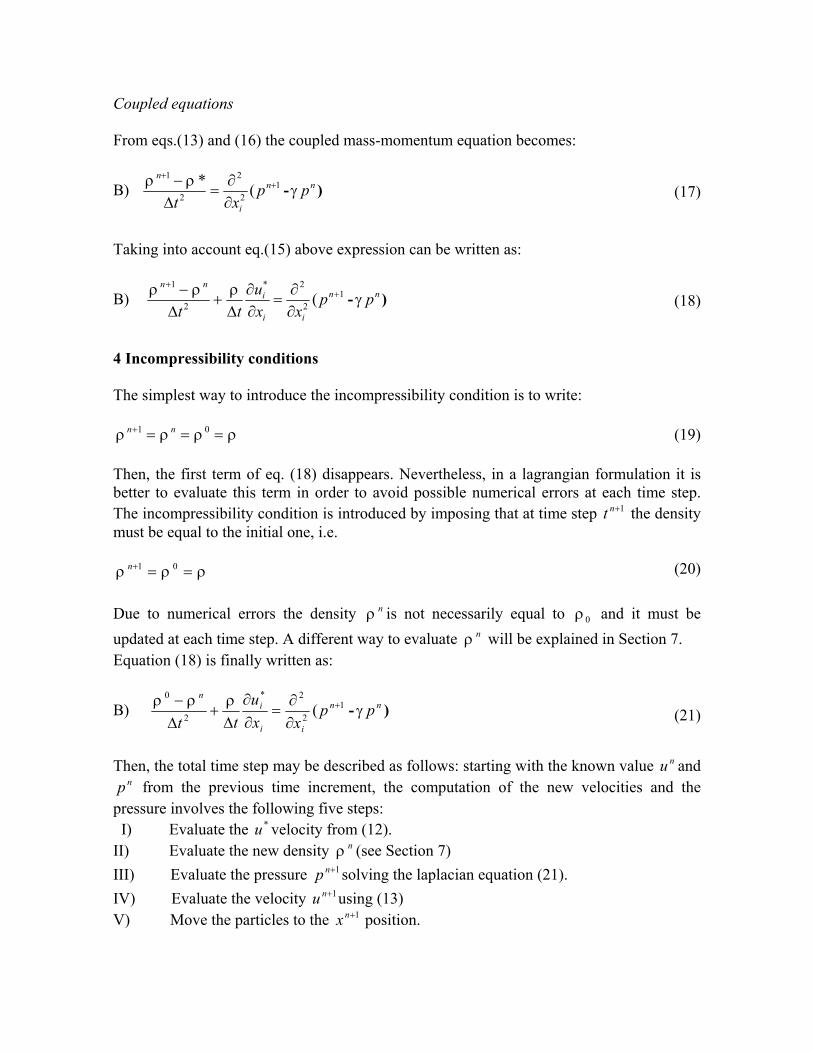
Coupled equations From eqs.(13) and (16) the coupled mass-momentum equation becomes:

B) )- nn

i

n

ppxt

γρρ 1

2

2

2

1

(* ++

∂∂

=∆− (17)

Taking into account eq.(15) above expression can be written as:

B) )- nn

ii

inn

ppxx

utt

γρρρ 1

2

2*

2

1

( ++

∂∂

=∂∂

∆+

∆− (18)

4 Incompressibility conditions The simplest way to introduce the incompressibility condition is to write:

ρρρρ ===+ 01 nn (19) Then, the first term of eq. (18) disappears. Nevertheless, in a lagrangian formulation it is better to evaluate this term in order to avoid possible numerical errors at each time step. The incompressibility condition is introduced by imposing that at time step 1+nt the density must be equal to the initial one, i.e.

ρρρ ==+ 01n (20) Due to numerical errors the density nρ is not necessarily equal to 0ρ and it must be updated at each time step. A different way to evaluate nρ will be explained in Section 7. Equation (18) is finally written as:

B) )- nn

ii

in

ppxx

utt

γρρρ 1

2

2*

2

0

( +

∂∂

=∂∂

∆+

∆−

(21) Then, the total time step may be described as follows: starting with the known value nu and

np from the previous time increment, the computation of the new velocities and the pressure involves the following five steps: I) Evaluate the *u velocity from (12).

II) Evaluate the new density nρ (see Section 7) III) Evaluate the pressure 1+np solving the laplacian equation (21). IV) Evaluate the velocity 1+nu using (13) V) Move the particles to the 1+nx position.

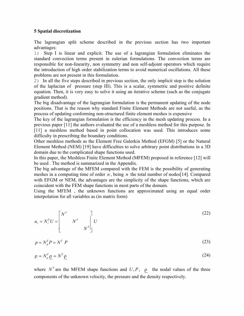
5 Spatial discretization The lagrangian split scheme described in the previous section has two important advantages: 1) Step I is linear and explicit. The use of a lagrangian formulation eliminates the standard convection terms present in eulerian formulations. The convection terms are responsible for non-linearity, non symmetry and non self-adjoint operators which require the introduction of high order stabilization terms to avoid numerical oscillations. All these problems are not present in this formulation. 2) In all the five steps described in previous section, the only implicit step is the solution of the laplacian of pressure (step III). This is a scalar, symmetric and positive definite equation. Then, it is very easy to solve it using an iterative scheme (such as the conjugate gradient method). The big disadvantage of the lagrangian formulation is the permanent updating of the node positions. That is the reason why standard Finite Element Methods are not useful, as the process of updating conforming non-structured finite element meshes is expensive The key of the lagrangian formulation is the efficiency in the mesh updating process. In a previous paper [11] the authors evaluated the use of a meshless method for this purpose. In [11] a meshless method based in point collocation was used. This introduces some difficulty in prescribing the boundary conditions. Other meshless methods as the Element Free Galerkin Method (EFGM) [5] or the Natural Element Method (NEM) [19] have difficulties to solve arbitrary point distributions in a 3D domain due to the complicated shape functions used. In this paper, the Meshless Finite Element Method (MFEM) proposed in reference [12] will be used . The method is summarized in the Appendix. The big advantage of the MFEM compared with the FEM is the possibility of generating meshes in a computing time of order n , being n the total number of nodes[14]. Compared with EFGM or NEM, the advantages are the simplicity of the shape functions, which are coincident with the FEM shape functions in most parts of the domain. Using the MFEM , the unknown functions are approximated using an equal order interpolation for all variables as (in matrix form)

UN

NN

UNuT

T

T

Tii

==

(22)

PNPNp TT

p == (23)

ρρρ ρ

TT NN == (24)

where TN are the MFEM shape functions and PU , , ρ the nodal values of the three components of the unknown velocity, the pressure and the density respectively.

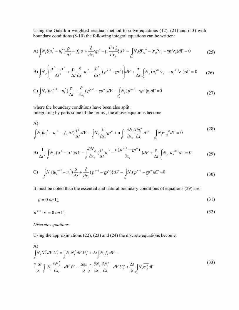
Using the Galerkin weighted residual method to solve equations (12), (21) and (13) with boundary conditions (8-10) the following integral equations can be written:

A) 0)(()( * =Γ−−−∂∂

−∂∂

+−∆

− ∫∫Γ

dpNdVx

px

ft

uuN in

jn

ijn

niij

nijn

ii

nii

Vi νγντσ

τµγρ

ρ

σ

(25)

B) 0)() -( 1112

2*

2

0

=Γ−∆

+

∂∂

−∂∂

∆+

∆−

∫∫Γ

+++ duuNt

dVppx

uxtt

Nu

in

iin

ipV

nn

ii

i

n

p ννρ

γρρρ

(26)

C) 0)(()( 11*1 ∫∫Γ

+++ =Γ−−−∂∂

+∆

−σ

νγγρ dppNdVpp

xtuuN i

nni

nn

ii

ni

Vi

(27)

where the boundary conditions have been also split. Integrating by parts some of the terms , the above equations become: A)

0)( * =Γ−∂∂

∂∂

+∂∂

+∆

∆−− ∫∫∫∫Γ

dNdVxu

xN

px

NdVt

tfuuN nnii

i

ni

i

i

VV

n

iii

nii

Vi

σ

σµγρ

(28)

B) 0) )(()(1 11

*02 =Γ

∆+

∂−∂

−∆∂

∂−−

∆ ∫∫∫Γ

++

duNt

dVx

pputx

NdVN

tu

nnp

V i

nn

ii

p

V

np

ργρρρ

(29)

C) 0)()()( 11*1 ∫∫Γ

+++ =Γ−−−∂∂

+∆

−σ

γγρ dppNdVpp

xtuuN nn

inn

ii

ni

Vi

(30)

It must be noted than the essential and natural boundary conditions of equations (29) are:

σΓ= onp 0 (31)

un onu Γ=⋅+ 01 ν (32)

Discrete equations Using the approximations (22), (23) and (24) the discrete equations become: A)

∫∫∫

∫∫∫

Γ

Γ∆

+∂∂

∂∂∆

−∂

∂∆

−∆+=

σ

σρρ

µρ

γdNtUdV

xN

xNtPdV

xN

Nt

dVfNtUdVNNUdVNN

nni

ni

i

Ti

i

i

V

n

i

Tp

iV

iV

ini

V

Tiii

V

Tii

*

(33)

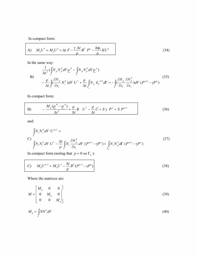
In compact form:

A) nnTnuu KUtPBtFtUMUM

ρµ

ργ ∆

−∆

−∆+=* (34)

In the same way:

B) ∫∫ ∫

∫∫

−∂

∂

∂

∂−=Γ

∆+

∂

∂

∆−

−∆

+

Γ

+

V

nn

i

Tp

i

p

V

nnp

Ti

i

p

V

nTp

V

Tpp

PPdVx

NxN

duNt

UdVNxN

t

dVNNdVNNt

u

)()()(

)(1

11*

02

γρρ

ρρ ρ

(35)

In compact form:

B) 1*2

0 )(+=+

∆−

∆+

∆

−− nn

np PSPSU

tUB

ttM

γρρρρ ) (36)

and:

C) )()( 11*

1

nnTpi

nn

i

Tp

Vi

Ti

Vi

nTi

Vi

PPdNNPPdVx

NNtUdVNN

UdVNN

γγρ

σ

−Γ+−∂

∂∆−

=

∫∫∫

∫

Γ

++

+

(37)

In compact form (noting that σΓ= onp 0 ):

C) )( 1*1 nnTu

nu PPBtUMUM γ

ρ−

∆−= ++ (38)

Where the matrices are:

=

p

p

p

MM

MM

000000

(39)

∫=V

Tp dVNNM (40)

∂∂

∂∂

∂∂

= ∫ ∫∫V V

T

V

TT dVNzNdVN

yNdVN

xNB )(;)(;)( (41)

dVz

NzN

yN

yN

xN

xNS

TT

V

T

)(∂∂

∂∂

+∂∂

∂∂

+∂∂

∂∂

= ∫ (42)

Γ= ∫

Γ

+ duNUu

nn

1) (43)

=

SS

SK

000000

(44)

+

=

∫∫∫

∫∫∫

V

nzT

V

nyT

V

nxT

Vz

T

Vy

T

Vx

TT

dVNdVNdVN

dVfNdVfNdVfNF

σσσρ

;;1

;;

(45)

6. Stabilization of the incompressibility condition In the Eulerian form of the momentum equations, the discrete form must be stabilized in order to avoid numerical wiggles in the velocity and pressure results. This is not the case in the lagrangian formulation where no stabilization parameter must be added in equations (34) and (38). Nevertheless, the incompressibility condition must be stabilized in equal-order approximations to avoid possible pressure oscillations. Then, equation (36) must be stabilized if smooth pressure results are important. It must be noted than pressure oscillations do not influence significantly in the velocity results. Nevertheless, in most physical problems, pressure is the main result to be obtained. That is why stabilization of equation (36) must be performed. The so-called finite calculus (FIC) formulation [20-22] will be choused here as the stabilization procedure. This formulation is based in the modification of the governing differential equations of the problem by accepting that the domain where the balance laws are established (balance of momentum and balance of mass) has a finite size. The modified equations in the FIC formulation for incompressible fluids are. Momentum

02

=∂∂

−k

iki x

rhr

(46)

Mass conservation

02

=∂∂

−k

k

xrh

r (47)

where from eq.(1) and (2) the residuals are defined by:

ij

ij

i

ii f

xxp

DtDu

r ρτ

ρ −∂

∂−

∂∂

+= (48)

i

i

xu

DtDr

∂∂

+= ρρ

(49)

with dnki ,1, = where dn are the space dimensions of the problem. Eqs. (46,47) are completed with the boundary and initial conditions. Note that for consistency, the Neumann boundary condition on σΓ must also be adequately modified by adding a residual term. The details can be found in [21]. The underlined terms in Eqs. (46,47) introduce the necessary stabilization in the numerical solution using whatever discretization method. Examples of the application of the FIC approach the convection-diffusion problems and incompressible problems in solids and fluid mechanics are presented in [21-22]. Distances ih in Eqs.(46,47) are “characteristic length” parameters and their values control the relevance of the stabilization terms. The computation of the characteristic lengths is a critical issue in the stabilization process [20]. The new terms in the momentum and mass conservation equations stabilize the numerical solution in presence of high values of the convective terms and incompressibility zones, respectively. Obviously, in lagrangian flows, as in incompressible solid mechanics problems, the relevant stabilization term is that of Eq.(47), as the convective terms are zero in the momentum equations. For the practical application of the FIC formulation the stabilization term in the mass balance equation is expressed as a function of the residual of the momentum equations using Eq.(46) as:

∑= ∂

∂≅

∂∂ dn

i i

ii

k

k

xr

xrh

12τ

(50)

where iτ are intrinsic time parameters given by:

µτ

83 2

ii

h=

(51)

The modified incompressibility equation is therefore written for the numerical computations as:

∑=

=∂∂

−dn

i i

ii x

rr

10τ

(52)

The stabilization terms in the momentum equation (46) are dropped hereonwards for the numerical solution. It is convenient to rewrite the residual ir in Eq.(48) as

ii

i xpr π+

∂∂

= (53)

where iπ are pressure gradient projection terms. These terms are considered as additional nodal variables. The necessary additional equations to match the increase in the number of unknowns are obtained by expressing that the residual ir as defined by Eq.(48), vanishes, in the average sense, over each element. This can be expressed in weighted integral form as

∫ =+∂∂

Vi

ii dV

xpw 0)( π

(54)

where iw are appropriate weighting functions. Discretization of the iπ terms using the same MFEM interpolation functions gives:

Π= Tii Nπ (55)

where Π represents the local value of the three components of the pressure gradient. Eq.(54) leads to an equation system of the form (for ii Nw = )

0=+Π PBM T (56) Eq.(21) is now modified with the new stabilization term as:

i1

12

2*

2

0

x )-(∂∂

∆+

∂∂

=∂∂

∆+

∆− ∑

=

+ in

i

inn

ii

in r

tpp

xxu

tt

d τγ

ρρρ (57)

and Eq.(26) becomes noww

+

∂∂

∆−

∂∂

−∂∂

∆+

∆−

∫ ∑=

+ dVr

tpp

xu

xttN

V

in

i

inn

ii

i

n

p

d

i1

12

2*

2

0

x ) -(

τγ

ρρρ boundary terms (58)

Integrating by parts, the equivalent to eq.(29) is:

0..)( )(

)(1

11

1

1*

02

=++∂∂

∆−

∂−∂

−∆∂

∂

−−∆

++

=

+

∑∫

∫

tbdVx

ptx

pputx

N

dVNt

ni

i

nn

i

i

V i

nn

ii

p

V

np

d

πτγρ

ρρ

(59)

Introducing the discretization of the different fields, and using a compact notation gives:

1*2

0

)()(

++=Π−+∆

−∆

+∆

−− nnn

np PSSBPSU

tUB

ttM

ττγρρρρ )

(60)

where the new stabilization matrices τB and τS are defined by:

∆∂∂

∆∂∂

∆∂∂

= ∫ ∫∫V V

zT

V

yTxT

tdVN

zN

tdVN

yN

tdVN

xNB τττ

τ )(;)(;)( (61)

dVtz

NzN

tyN

yN

txN

xNS z

Ty

Tx

V

T

)(∆∂

∂∂∂

+∆∂

∂∂∂

+∆∂

∂∂∂

= ∫τττ

τ (62)

Note that the effect of the stabilization terms is the addition of a new Laplacian matrix

τS and a new term in the r.h.s. of Eq.(60) depending on the pressure gradient projection variables iπ . The pressure gradient projection may be evaluated explicitly using eq.(56) by: D) 111 +−+ −=Π nTn PBM (63) The three steps A),B),C) described before are now completed with a fourth step D) where the lumped diagonal form of matrix M may be used. 7. Mass conservation In a lagrangian formulation a new mesh is generated at each time step, and all the information is transmitted with the nodes or particles. In that way, a local variation in the volume associated with the particles is used as the correct volume in the next time step. A permanent update of the initial volume is necessary to avoid large error accumulation. Thus, the correct evaluation of the first term of equation (36) becomes important in a lagrangian formulation and will be discussed below. The term

)( 0 npM ρρ − (64)

may be evaluated in two different ways:

I) Evaluation via a density update From the mass conservation equation, the density at time nt may be computed as:

i

ninn

xut∂∂

∆−= − ρρρ 1 (65)

Making use of the spatial discretization (22) and (24) and the Galerkin residual method gives:

n

i

Ti

Vp

nTp

Vp

nTp

Vp UdV

xNNtdVNNdVNN∂∂

∆−= ∫∫∫ − ρρρ 1 (66)

Integrating by parts the last term:

∫∫∫∫Γ

− Γ∆−∂

∂∆+=

u

duNtUdVNx

NtdVNNdVNN n

npnT

ii

Tp

V

nTp

Vp

nTp

Vp ρρρρ 1 (67)

or in compact notation:

UtUBtMM nnp

np

ˆ1 ∆−∆+= − ρρρρ (68)

In order to take into account that the shape functions N are different at each mesh update the following notation will be used: the shape functions or the matrices evaluated at the time nt will be noted by n

pN and npM . Then equation (68) becomes:

nnnnnn

pnn

p UtUBtMM ˆ1 ∆−∆+= − ρρρρ (69)

where tn∆ represents the time increment al time nt Then:

ρρρρρρ nnnnnnp

nnn UtUBMt ∆+=∆−∆+= −−− 111 ˆ)( (70)

where the density variation has been defined by:

nnnnp

nn UtUBMt ˆ)( 1 ∆−∆=∆ − ρρρ (71)

representing the ρ variation at time nt . Successive application of eq.(70) for all time steps gives:

lln

l

lllp

ln

l

ln UtUBMt ˆ)(1

10

1

0 ∆−∆+=∆+= ∑∑=

−

=

ρρρρρ (72)

The term )( 0 npM ρρ − of the r.h.s. of Eq.(36) can be written as:

∑=

∆−=−n

l

lp

np MM

1

0 )( ρρρ (73)

This means that at each time step lt the vector:

lllllp

ll UtUBMt ˆ)( 1 ∆−∆=∆ −ρρ (74)

must be evaluated, added to the previous one and stored for the next time step. II) Evaluation via the initial associated volume Mass conservation implies:

∫∫==

=)()0(

0

ntt V

n

V

dVdV ρρ (75)

Using the shape functions at the corresponding time step:

n

V

Tn

V

T

ntt

dVNdVN ρρ ρρ ∫∫==

=)()0(

)()( 00 (76)

Defining the volume associated to each particle by:

∫=

=Ω)(

)()(ntV

TnTn dVN ρ (77)

eq.(76) becomes:

nTnT ρρ )()( 00 Ω=Ω (78)

which has the meaning of the total mass conservation. Vector nΩ may be considered as the vector containing the volumes associated to each particle. It may be calculated using (77) or using the Voronoi diagram of the node distribution. The concept of local mass conservation may be used next. This means that each particle (node) conserves his own local mass, i.e.:

ni

niii ρρ Ω=Ω 00 (79)

The term )( 0 n

pM ρρ − may be written as:

)()( 000000 Ω−Ω=Ω−Ω=−Ω nnnn ρρρρρ (80)

where 0Ω and nΩ represent a diagonal matrix with the volume associated to each particle

at time 0tt = and ntt = respectively. These matrices may be evaluated using the lumped matrices 0

ρM and nM ρ or directly using the associated volume to each particle obtained from a Voronoi diagram. 8. Boundary Surfaces One of the main problems in mesh generation is the correct definition of the boundary domain. Sometimes, boundary nodes are explicitly defined as special nodes, which are different from internal nodes. In other cases, the total set of nodes is the only information available and the algorithm must recognize the boundary nodes. Such is the case in the lagrangian formulation in which, at each time step, a new node distribution is obtained and the boundary-surface must be recognized from the node positions. The use of the MFEM with the Extended Delaunay partition makes it easier to recognize boundary nodes. Considering that the node follows a variable )(xh distribution, where )(xh is the minimum distance between two nodes, the following criterion has been used: All nodes on an empty sphere with a radius )(xr bigger than )(xhα , are considered as boundary nodes. Thus, α is a parameter close to, but greater than one. Note that this criterion is coincident with the Alpha Shape concept [12]. Once a decision has been made concerning which of the nodes are on the boundaries, the boundary surface must be defined. It is well known that in 3-D problems the surface fitting a number of nodes is not unique. For instance, four boundary nodes on the same sphere may define two different boundary surfaces, a concave one and convex one. In this work, the boundary surface is defined with all the polyhedral surfaces having all their nodes on the boundary and belonging to just one polyhedron. See Reference [12]. The correct boundary surface may be important to define the correct normal external to the surface. Furthermore; in weak forms (Galerkin) a correct evaluation of the volume domain is also important. Nevertheless, it must be noted that in the criterion proposed above, the error in the boundary surface definition is of order h . This is the standard error of the boundary surface definition in a meshless method for a given node distribution. 9. Application to Fluid-Structure Interactions The fluid described above will interact with structures that are in contact with it. Three different cases of structures will be analyzed. In all three cases, the elastic strains will be neglected and only rigid solid motions will be considered.

Fixed structures The first type of examples presented is structures in which there is a fixed wall, for instance, the recipient in which the fluid is contained. See Figs. 1 and 2. This kind of structures will be analyzed by adding fixed particles at the boundaring with velocity 0=iu . These particles will be included in the computation of equations A) and B) as standard nodes, but during the equation C) the velocity will be fixed to zero. The inclusion of fixed boundary particles is very important to avoid contact problems. These fixed particles automatically force the fluid to remain inside a recipient. The moving particles cannot go across the wall due to the incompressibility condition and not to any other restriction of velocity or displacement. This condition solves the contact problems with complicated curved structures. See for instance example 2. Moving structures with a known velocity The second type of fluid-structure interaction is between the fluid and a moving wall of known velocity as a function of the time. This is the case of moving recipients, moving mills, or moving ships with prescribed velocity. In this case, moving particles with known velocity are introduced in the domain boundaries. Note that the term:

Ut)

∆ρ

(81)

with

Γ= ∫Γ

+ duNUu

nn

1) (82)

must be added in equation C) where 1+n

nu are the known velocity on the boundaries. See for instance Figs. 4 and 5. Moving structures Finally, the case of moving rigid structures is considered. For instance, the case of a floating ship originating to water waves (see keeping). In this case, the solid will be considered as a domain with a high viscosity parameter, much higher than the fluid domain. For practical problems a value of µ410 is enough to represent a solid without introducing numerical problems (see Figures 5 and 6). 10 Numerical Test 10.1 Water column collapse

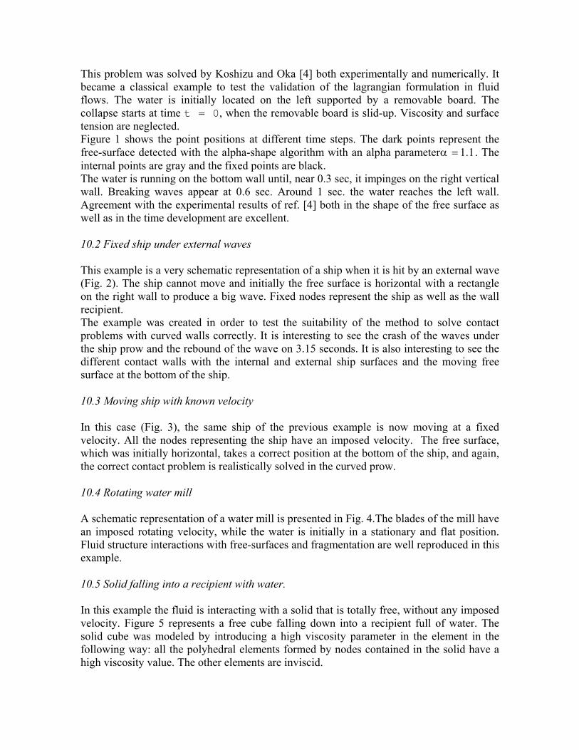
This problem was solved by Koshizu and Oka [4] both experimentally and numerically. It became a classical example to test the validation of the lagrangian formulation in fluid flows. The water is initially located on the left supported by a removable board. The collapse starts at time t = 0, when the removable board is slid-up. Viscosity and surface tension are neglected. Figure 1 shows the point positions at different time steps. The dark points represent the free-surface detected with the alpha-shape algorithm with an alpha parameter 1.1=α . The internal points are gray and the fixed points are black. The water is running on the bottom wall until, near 0.3 sec, it impinges on the right vertical wall. Breaking waves appear at 0.6 sec. Around 1 sec. the water reaches the left wall. Agreement with the experimental results of ref. [4] both in the shape of the free surface as well as in the time development are excellent. 10.2 Fixed ship under external waves This example is a very schematic representation of a ship when it is hit by an external wave (Fig. 2). The ship cannot move and initially the free surface is horizontal with a rectangle on the right wall to produce a big wave. Fixed nodes represent the ship as well as the wall recipient. The example was created in order to test the suitability of the method to solve contact problems with curved walls correctly. It is interesting to see the crash of the waves under the ship prow and the rebound of the wave on 3.15 seconds. It is also interesting to see the different contact walls with the internal and external ship surfaces and the moving free surface at the bottom of the ship. 10.3 Moving ship with known velocity In this case (Fig. 3), the same ship of the previous example is now moving at a fixed velocity. All the nodes representing the ship have an imposed velocity. The free surface, which was initially horizontal, takes a correct position at the bottom of the ship, and again, the correct contact problem is realistically solved in the curved prow. 10.4 Rotating water mill A schematic representation of a water mill is presented in Fig. 4.The blades of the mill have an imposed rotating velocity, while the water is initially in a stationary and flat position. Fluid structure interactions with free-surfaces and fragmentation are well reproduced in this example. 10.5 Solid falling into a recipient with water. In this example the fluid is interacting with a solid that is totally free, without any imposed velocity. Figure 5 represents a free cube falling down into a recipient full of water. The solid cube was modeled by introducing a high viscosity parameter in the element in the following way: all the polyhedral elements formed by nodes contained in the solid have a high viscosity value. The other elements are inviscid.

The example represents correctly the contact problem when the cube hits the water and also the different speed during the falling process. 10.6 Solid floating on a free surface The last example of Figure 6 represents a very interesting problem of fluid structure interaction when there is a weak interaction between the fluid and a large rigid deformation of the structure. In this case, there is also a free-surface problem, representing a schematic case of see-keeping in ship hydrodynamics. The example shows an initially stationary recipient with a floating piece of wood in which a wave is produced on the left side. The wave intercepts the wood piece producing a breaking wave and moving the floating wood. All the previous examples are only schematic representations of real problems. Only the first example has an experimental reference. The rest are presented here in order toe evaluate the suitability of the method to solve problems other methods have difficulties to solve. 11 Conclusions Lagrangian formulation and the Meshless Finite Element Method are an excellent combination to solve fluid mechanic problems, especially fluid-structure interactions with moving free-surface and contact problems. Breaking waves, collapse problems, and contact problems can be solved easily without any additional constraint. Furthermore, the Meshless Finite Element Method presented, as opposed to other methods, has the advantages of a good meshless method concerning the easy introduction of the nodes connectivity in a bounded time of order n . The method proposed also shares some advantages with the FEM such as: a) the simplicity of the shape functions, b) 0C continuity between elements, c) an easy introduction of the boundary conditions, and d) symmetric matrices. The Finite Calculus (FIC) formulation can be successfully used in a lagrangian formulation in order to eliminate spurious pressure oscillations. Both the lagrangian formulation and the MFEM are the key ingredients to solve fluid-structure interaction problems including with free-surface, breaking waves and collapse situations.

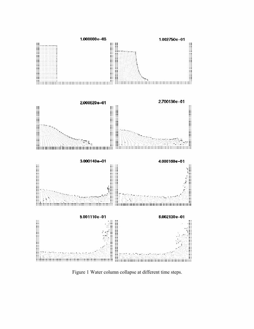
Figure 1 Water column collapse at different time steps.

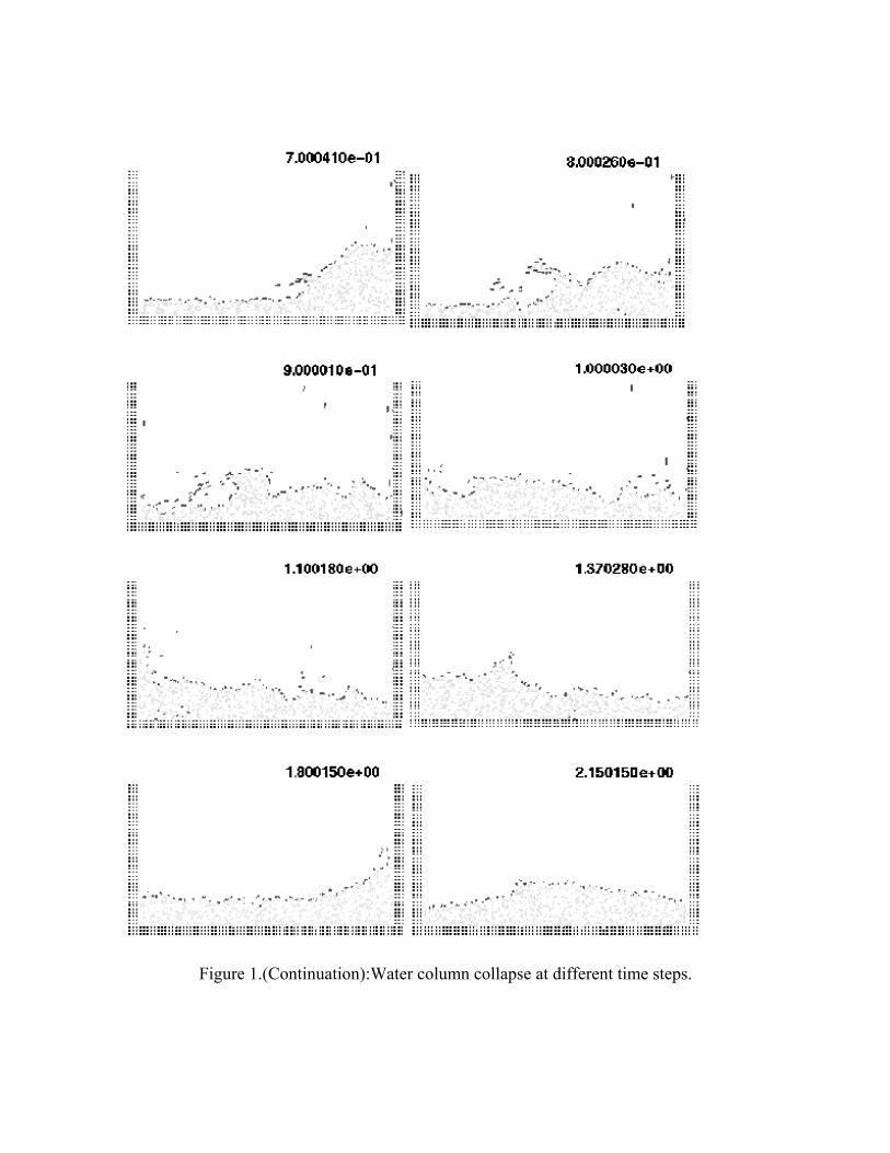
Figure 1.(Continuation):Water column collapse at different time steps.

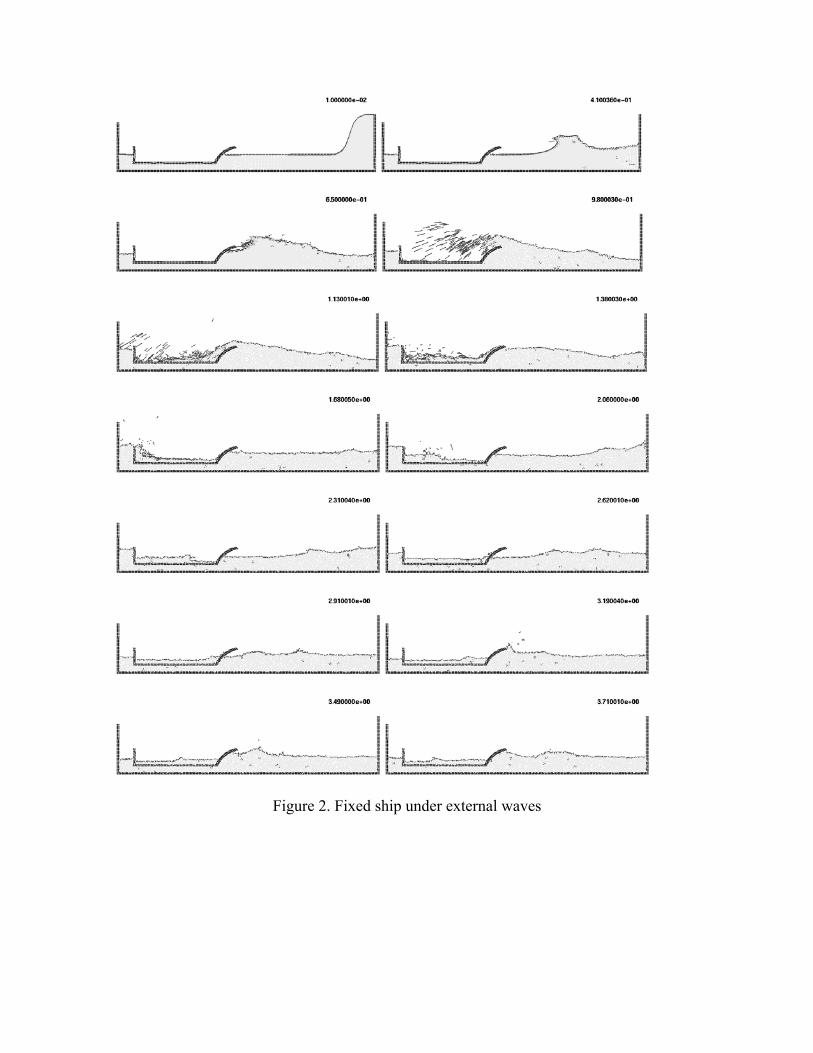
Figure 2. Fixed ship under external waves

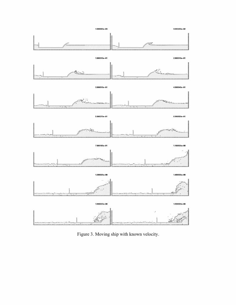
Figure 3. Moving ship with known velocity.

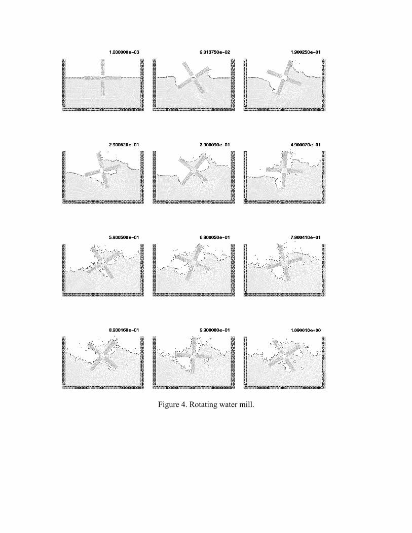
Figure 4. Rotating water mill.

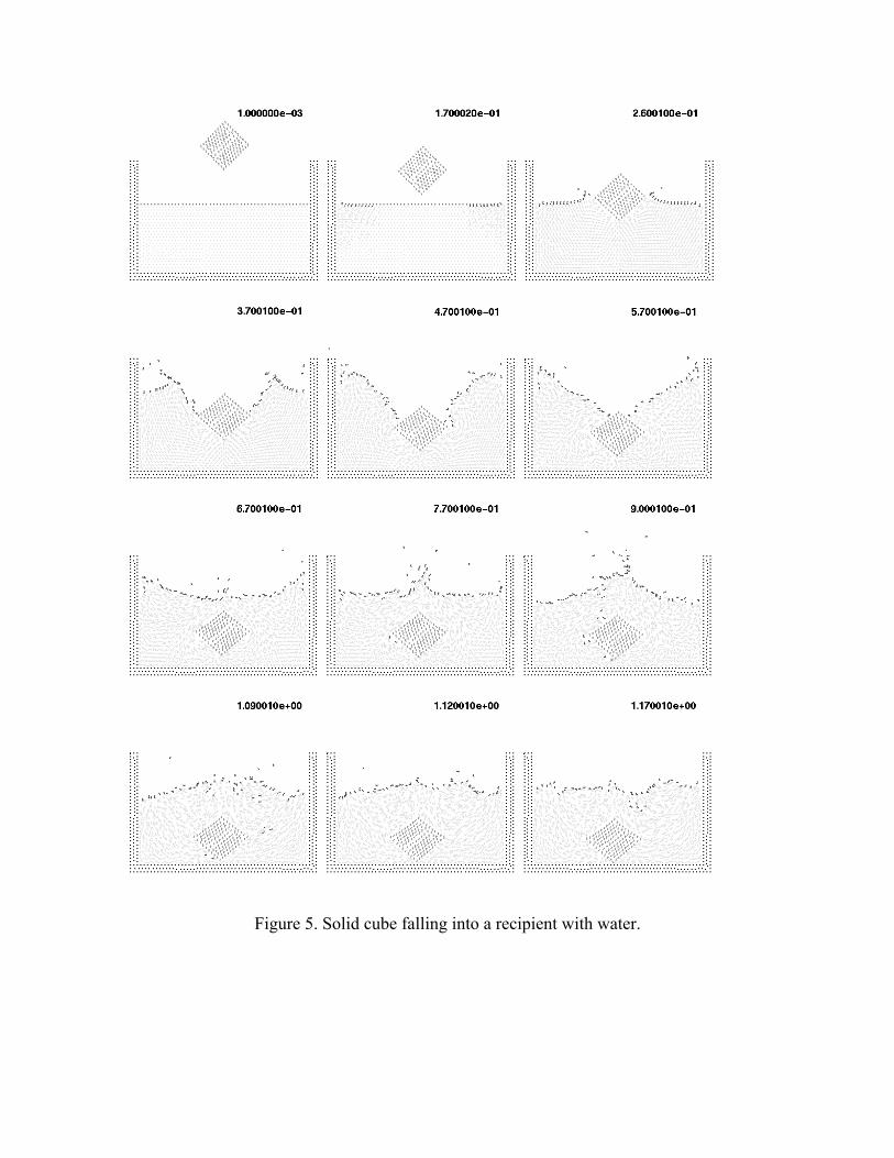
Figure 5. Solid cube falling into a recipient with water.

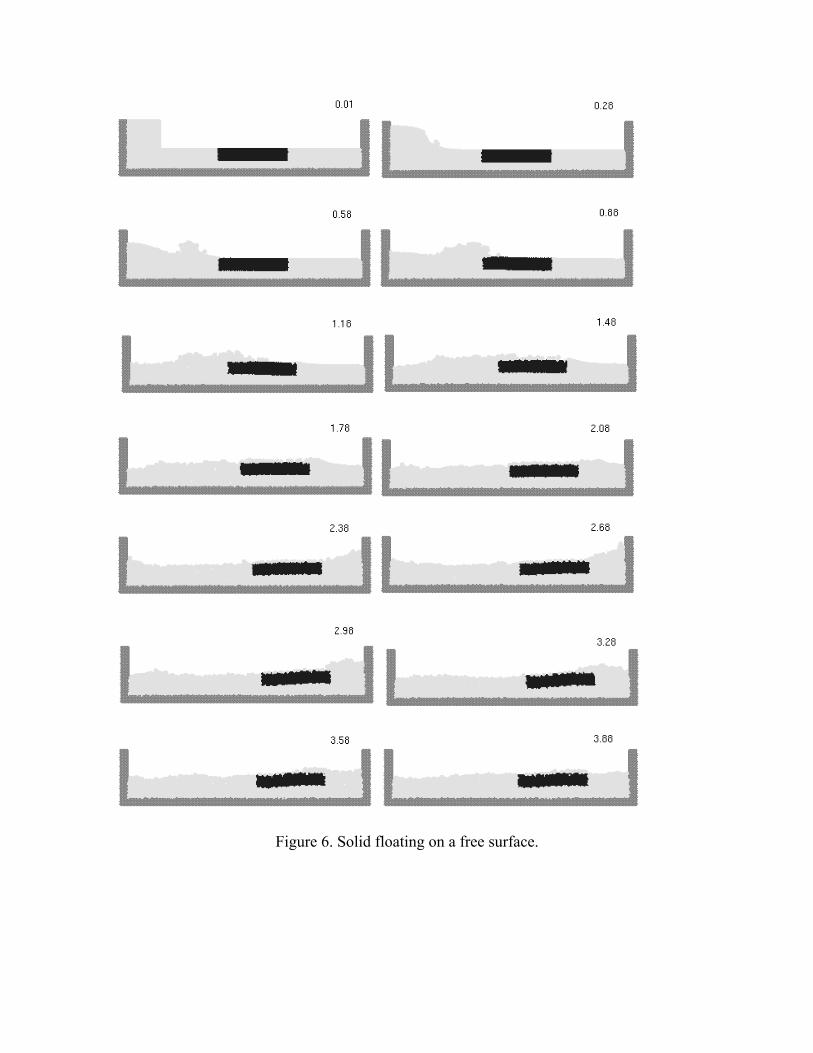
Figure 6. Solid floating on a free surface.

Appendix

All the shape functions iN described in this paper are based on the Meshless Finite Element Method (MFEM). A full description of the MFEM may be found in Ref. [12]. Nevertheless and for the sake of completeness a summary is presented in this Appendix.

The MFEM combines a particular finite element subdivision in polyhedral shape called the Extended Delanay Tessellation and ad-hoc shape functions for this kind of polyhedra. The Extended Delaunay Tessellation (EDT) Let a set of distinct nodes be: N = n1, n2, n3,…,nn in R3.

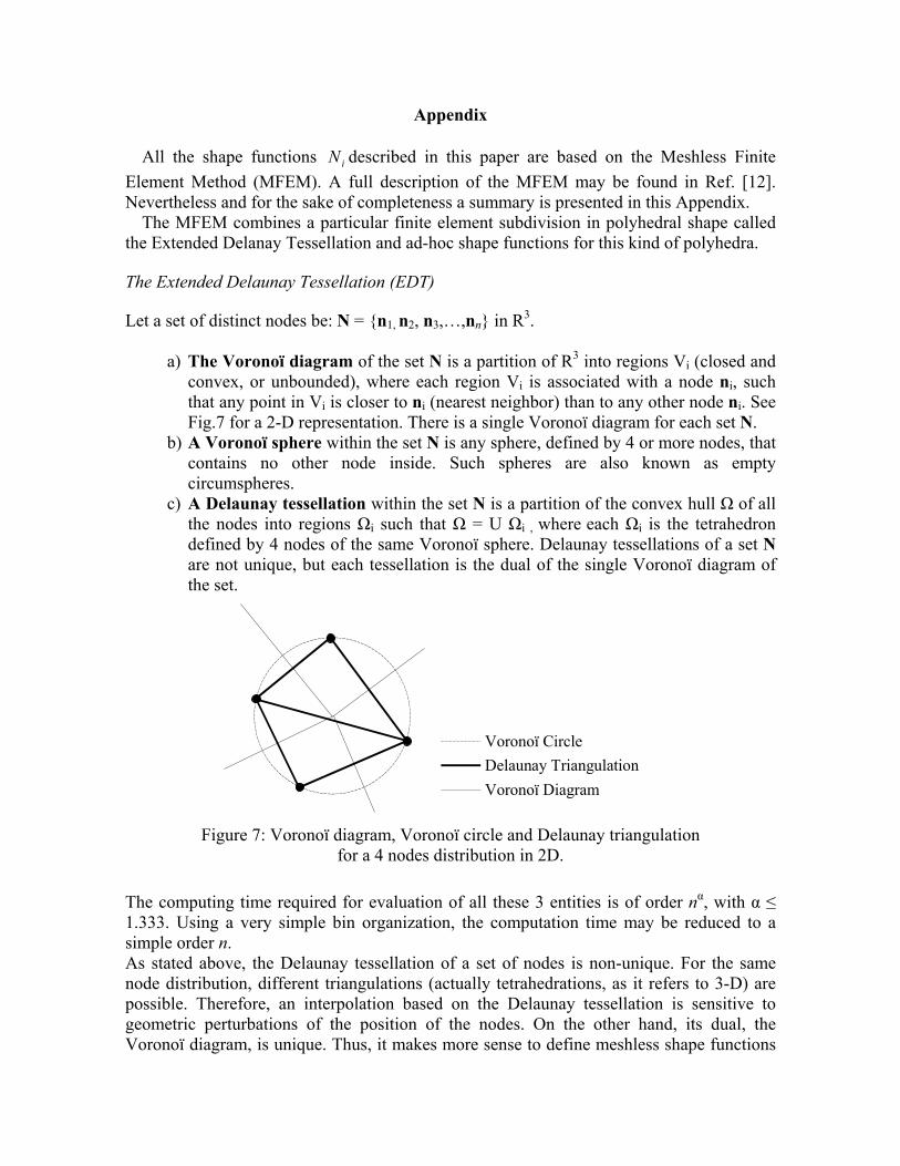
a) The Voronoï diagram of the set N is a partition of R3 into regions Vi (closed and convex, or unbounded), where each region Vi is associated with a node ni, such that any point in Vi is closer to ni (nearest neighbor) than to any other node ni. See Fig.7 for a 2-D representation. There is a single Voronoï diagram for each set N.

b) A Voronoï sphere within the set N is any sphere, defined by 4 or more nodes, that contains no other node inside. Such spheres are also known as empty circumspheres.

c) A Delaunay tessellation within the set N is a partition of the convex hull Ω of all the nodes into regions Ωi such that Ω = U Ωi , where each Ωi is the tetrahedron defined by 4 nodes of the same Voronoï sphere. Delaunay tessellations of a set N are not unique, but each tessellation is the dual of the single Voronoï diagram of the set.

Voronoï CircleDelaunay TriangulationVoronoï Diagram

Figure 7: Voronoï diagram, Voronoï circle and Delaunay triangulation

for a 4 nodes distribution in 2D.

The computing time required for evaluation of all these 3 entities is of order nα, with α ≤ 1.333. Using a very simple bin organization, the computation time may be reduced to a simple order n. As stated above, the Delaunay tessellation of a set of nodes is non-unique. For the same node distribution, different triangulations (actually tetrahedrations, as it refers to 3-D) are possible. Therefore, an interpolation based on the Delaunay tessellation is sensitive to geometric perturbations of the position of the nodes. On the other hand, its dual, the Voronoï diagram, is unique. Thus, it makes more sense to define meshless shape functions

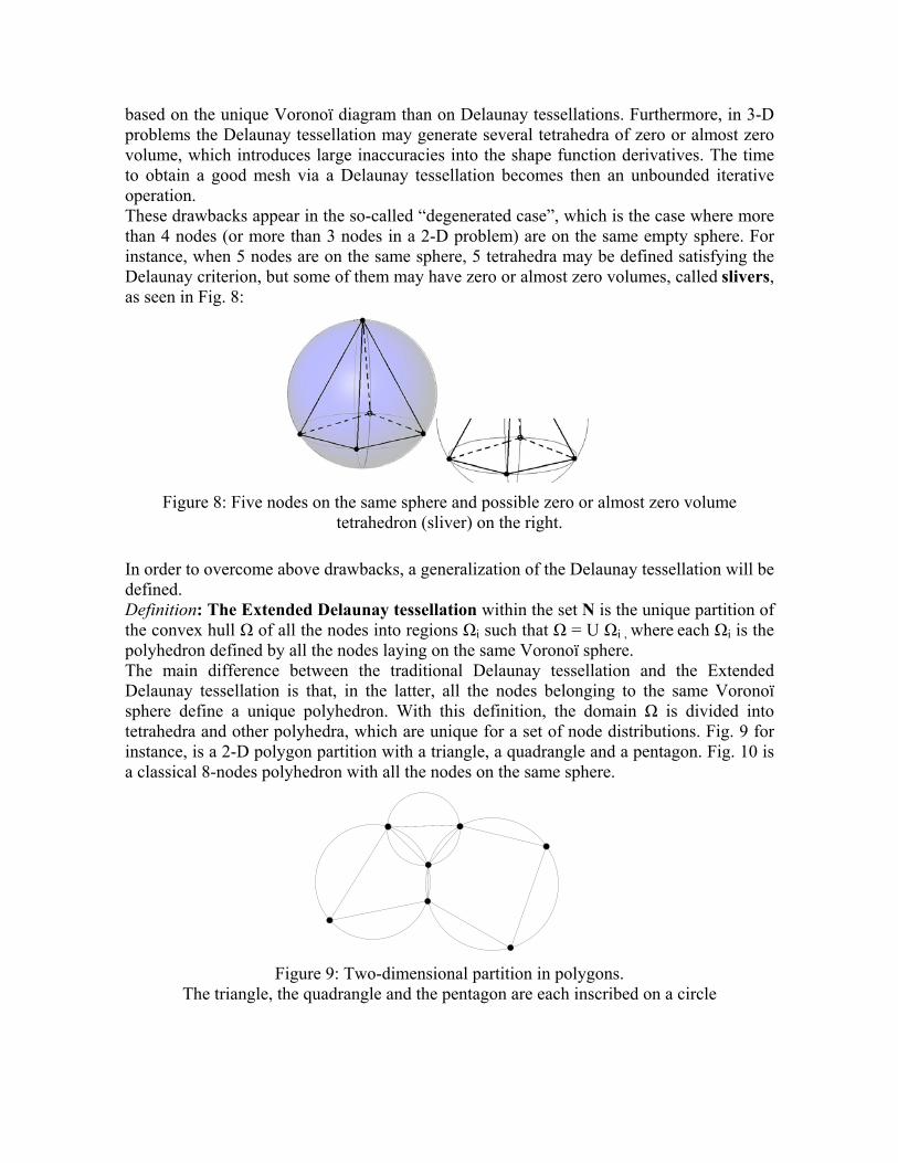
based on the unique Voronoï diagram than on Delaunay tessellations. Furthermore, in 3-D problems the Delaunay tessellation may generate several tetrahedra of zero or almost zero volume, which introduces large inaccuracies into the shape function derivatives. The time to obtain a good mesh via a Delaunay tessellation becomes then an unbounded iterative operation. These drawbacks appear in the so-called “degenerated case”, which is the case where more than 4 nodes (or more than 3 nodes in a 2-D problem) are on the same empty sphere. For instance, when 5 nodes are on the same sphere, 5 tetrahedra may be defined satisfying the Delaunay criterion, but some of them may have zero or almost zero volumes, called slivers, as seen in Fig. 8:

Figure 8: Five nodes on the same sphere and possible zero or almost zero volume

tetrahedron (sliver) on the right.

In order to overcome above drawbacks, a generalization of the Delaunay tessellation will be defined. Definition: The Extended Delaunay tessellation within the set N is the unique partition of the convex hull Ω of all the nodes into regions Ωi such that Ω = U Ωi , where each Ωi is the polyhedron defined by all the nodes laying on the same Voronoï sphere. The main difference between the traditional Delaunay tessellation and the Extended Delaunay tessellation is that, in the latter, all the nodes belonging to the same Voronoï sphere define a unique polyhedron. With this definition, the domain Ω is divided into tetrahedra and other polyhedra, which are unique for a set of node distributions. Fig. 9 for instance, is a 2-D polygon partition with a triangle, a quadrangle and a pentagon. Fig. 10 is a classical 8-nodes polyhedron with all the nodes on the same sphere.

Figure 9: Two-dimensional partition in polygons.

The triangle, the quadrangle and the pentagon are each inscribed on a circle

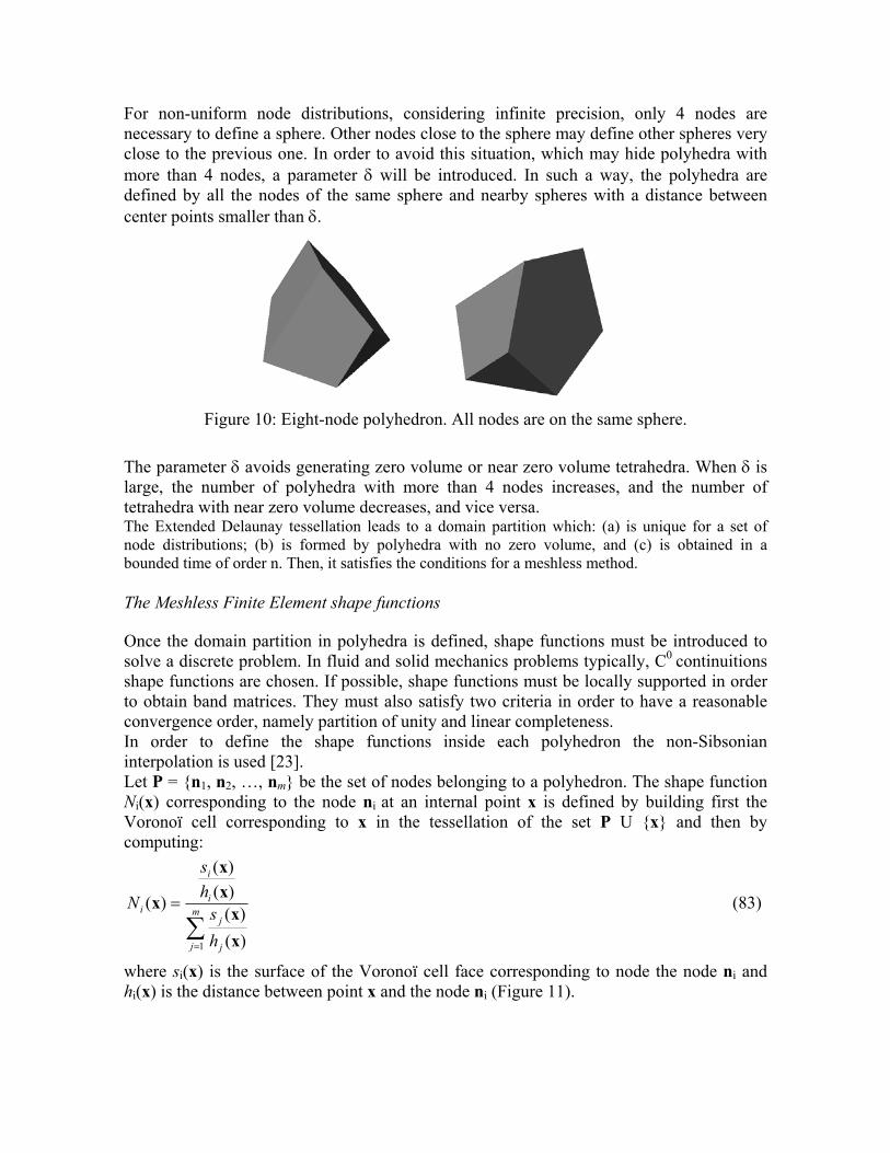
For non-uniform node distributions, considering infinite precision, only 4 nodes are necessary to define a sphere. Other nodes close to the sphere may define other spheres very close to the previous one. In order to avoid this situation, which may hide polyhedra with more than 4 nodes, a parameter δ will be introduced. In such a way, the polyhedra are defined by all the nodes of the same sphere and nearby spheres with a distance between center points smaller than δ.

Figure 10: Eight-node polyhedron. All nodes are on the same sphere.

The parameter δ avoids generating zero volume or near zero volume tetrahedra. When δ is large, the number of polyhedra with more than 4 nodes increases, and the number of tetrahedra with near zero volume decreases, and vice versa. The Extended Delaunay tessellation leads to a domain partition which: (a) is unique for a set of node distributions; (b) is formed by polyhedra with no zero volume, and (c) is obtained in a bounded time of order n. Then, it satisfies the conditions for a meshless method. The Meshless Finite Element shape functions Once the domain partition in polyhedra is defined, shape functions must be introduced to solve a discrete problem. In fluid and solid mechanics problems typically, C0

continuitions shape functions are chosen. If possible, shape functions must be locally supported in order to obtain band matrices. They must also satisfy two criteria in order to have a reasonable convergence order, namely partition of unity and linear completeness. In order to define the shape functions inside each polyhedron the non-Sibsonian interpolation is used [23]. Let P = n1, n2, …, nm be the set of nodes belonging to a polyhedron. The shape function Ni(x) corresponding to the node ni at an internal point x is defined by building first the Voronoï cell corresponding to x in the tessellation of the set P U x and then by computing:

∑=

=m

j j

j

i

i

i

hs

hs

N

1 )()(

)()(

)(

xx

xx

x (83)

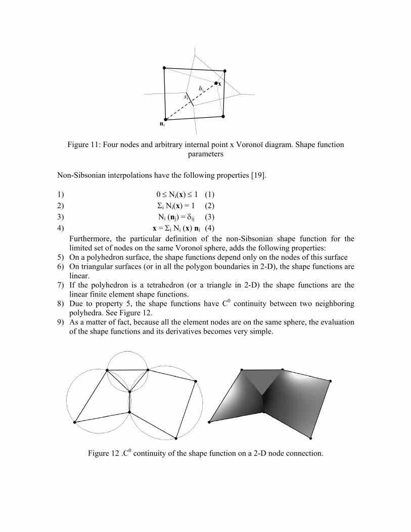
where si(x) is the surface of the Voronoï cell face corresponding to node the node ni and hi(x) is the distance between point x and the node ni (Figure 11).

x

ni

si

hi

Figure 11: Four nodes and arbitrary internal point x Voronoï diagram. Shape function

parameters

Non-Sibsonian interpolations have the following properties [19]. 1) 0 ≤ Ni(x) ≤ 1 (1) 2) Σi Ni(x) = 1 (2) 3) Ni (nj) = δij (3) 4) x = Σi Ni (x) ni (4)

Furthermore, the particular definition of the non-Sibsonian shape function for the limited set of nodes on the same Voronoï sphere, adds the following properties:

5) On a polyhedron surface, the shape functions depend only on the nodes of this surface 6) On triangular surfaces (or in all the polygon boundaries in 2-D), the shape functions are

linear. 7) If the polyhedron is a tetrahedron (or a triangle in 2-D) the shape functions are the

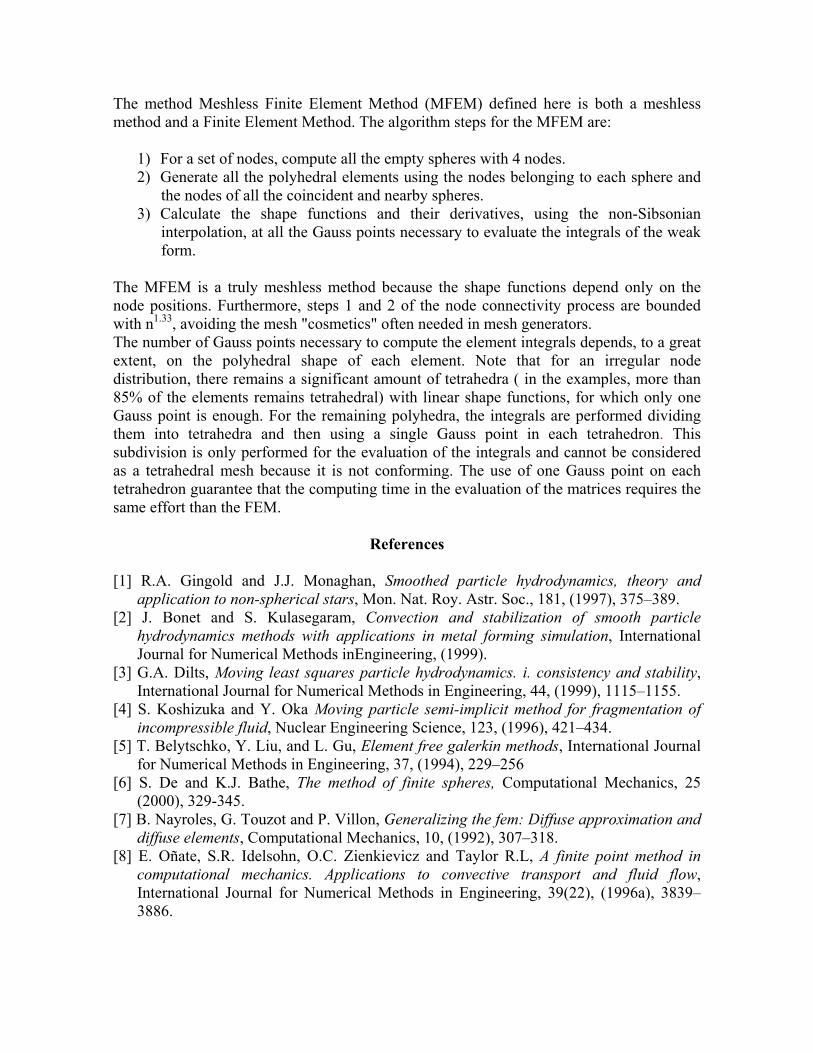
linear finite element shape functions. 8) Due to property 5, the shape functions have C0 continuity between two neighboring

polyhedra. See Figure 12. 9) As a matter of fact, because all the element nodes are on the same sphere, the evaluation

of the shape functions and its derivatives becomes very simple.

Figure 12 .C0 continuity of the shape function on a 2-D node connection.

The method Meshless Finite Element Method (MFEM) defined here is both a meshless method and a Finite Element Method. The algorithm steps for the MFEM are:

1) For a set of nodes, compute all the empty spheres with 4 nodes. 2) Generate all the polyhedral elements using the nodes belonging to each sphere and

the nodes of all the coincident and nearby spheres. 3) Calculate the shape functions and their derivatives, using the non-Sibsonian

interpolation, at all the Gauss points necessary to evaluate the integrals of the weak form.

The MFEM is a truly meshless method because the shape functions depend only on the node positions. Furthermore, steps 1 and 2 of the node connectivity process are bounded with n1.33, avoiding the mesh "cosmetics" often needed in mesh generators. The number of Gauss points necessary to compute the element integrals depends, to a great extent, on the polyhedral shape of each element. Note that for an irregular node distribution, there remains a significant amount of tetrahedra ( in the examples, more than 85% of the elements remains tetrahedral) with linear shape functions, for which only one Gauss point is enough. For the remaining polyhedra, the integrals are performed dividing them into tetrahedra and then using a single Gauss point in each tetrahedron. This subdivision is only performed for the evaluation of the integrals and cannot be considered as a tetrahedral mesh because it is not conforming. The use of one Gauss point on each tetrahedron guarantee that the computing time in the evaluation of the matrices requires the same effort than the FEM.

References

[1] R.A. Gingold and J.J. Monaghan, Smoothed particle hydrodynamics, theory and application to non-spherical stars, Mon. Nat. Roy. Astr. Soc., 181, (1997), 375–389.

[2] J. Bonet and S. Kulasegaram, Convection and stabilization of smooth particle hydrodynamics methods with applications in metal forming simulation, International Journal for Numerical Methods inEngineering, (1999).

[3] G.A. Dilts, Moving least squares particle hydrodynamics. i. consistency and stability, International Journal for Numerical Methods in Engineering, 44, (1999), 1115–1155.

[4] S. Koshizuka and Y. Oka Moving particle semi-implicit method for fragmentation of incompressible fluid, Nuclear Engineering Science, 123, (1996), 421–434.

[5] T. Belytschko, Y. Liu, and L. Gu, Element free galerkin methods, International Journal for Numerical Methods in Engineering, 37, (1994), 229–256

[6] S. De and K.J. Bathe, The method of finite spheres, Computational Mechanics, 25 (2000), 329-345.

[7] B. Nayroles, G. Touzot and P. Villon, Generalizing the fem: Diffuse approximation and diffuse elements, Computational Mechanics, 10, (1992), 307–318.

[8] E. Oñate, S.R. Idelsohn, O.C. Zienkievicz and Taylor R.L, A finite point method in computational mechanics. Applications to convective transport and fluid flow, International Journal for Numerical Methods in Engineering, 39(22), (1996a), 3839–3886.

[9] E. Oñate, S.R. Idelsohn, O.C. Zienkievicz, Taylor R.L. and C. Sacco, A stabilized finite point method for analysis of fluid mechanics problems, Computer Methods in Applied Mechanics and Engineering, 39, (1996a), 315–346.

[10] R.L. Taylor, O.C. Zienkiewicz, E. Oñate, and S.R. Idelsohn, Moving least square approximations for solution of differential equations, Internal Report 74, CIMNE, Barcelona, Spain, (1996).

[11] S.R. Idelsohn, M.A. Storti and E. Oñate, Lagrangian formulations to solve free surface incompressible inviscid fluid flows, Comput. Methods Appl. Mech. Engrg. 191,(2001) 583-593

[12] S.R. Idelsohn, E. Oñate, N. Calvo and F. Del Pin, The meshless finite element method, Submitted to Int. J. for Numerical Methods in Engineering, (2001).

[13] H. Edelsbrunner and E.P. Mucke, Three-dimensional alpha-shape. ACM Transactions on Graphics, 3, (1994), 43–72.

[14] N. Calvo, S.R. Idelsohn and E. Oñate, The extended Delaunay tesselation, Submitted to Computer Method in Applied Mechanics and Engineering, (2002).20

[15] K.J.Bathe, H.Zhang and S.Ji, Finite element analysis of fluid flows coupled with structural interactions, Comp. and Structures 72 (1999) 1-16

[16] H.Zhang and K.J.Bathe, Direct and iterative computing of fluid flows fully coupled with structures., Comput. Fluid and Solid Mechanics, (2001), 1440-1443.

[17] S.Rugonyi and K.J.Bathe, , CMES, Vol 2, No2, (2001) 195-212. [18] R.Codina, Pressure Stability in fractional step finite element methods for

incompressible flows, Journal of Comput. Phisycs, 170,(2001) 112-140. [19] Sukumar N, Moran B, Semenov AYu and Belikov VV. Natural neighbour Galerkin

Methods. International Journal for Numerical Methods in Engineering. 2001; 50:1-27. [20] E. Oñate Derivation of stabilized equations for advective-diffusive transport and fluid

flow problems. Comput. Methods Appl. Mech. Engrg.,1998, 151:1-2, 233--267. [21] E. Oñate. A stabilized finite element method for incompressible viscous flows using a

finite increment calculus formulation. Comput. Methods Appl. Mech. Engrg.,2000, 182:1--2, 355--370.

[22] E. Oñate, Possibilities of finite calculus in computational mechanics. (2002) Submitted to Int. J. Num. Meth. Engng.

[23] Belikov V and Semenov, A. Non-Sibsonian interpolation on arbitrary system of points in Euclidean space and adaptive generating isolines algorithm. Numerical Grid Generation in Computational Field Simulation, Proc. of the 6th Intl. Conf. Greenwich Univ. July 1998.