a mathematical history of taffy pullersa mathematical history of taffy pullers 2 2. some history the...

A MATHEMATICAL HISTORY OF TAFFY PULLERS

JEAN-LUC THIFFEAULT

Abstract. We describe a number of devices for pulling candy, called taffy pullers,that are related to pseudo-Anosov mapping classes. Though the mathematicalconnection has long been known for the two most common taffy puller designs,we unearth a rich variety of early designs from the patent literature.

1. Introduction

Taffy is a type of candy made by first heating sugar to a critical temperature,letting the mixture cool on a slab, then repeatedly ‘pulling’ — stretching andfolding — the resulting mass. The purpose of pulling is to get air bubbles into thetaffy, which gives it a nicer texture. Until the late 19th century, taffy was pulled byhand — an arduous task. The process was ripe for mechanization.

In the first decades of the 20th century there was a flurry of patents for taffypullers, with many displaying innovative ideas. These were designed to repeat-edly stretch and fold the taffy in a manner that would lead to exponential growth.What concerns us most here is their mathematical underpinning: we will showthat the computation of the growth of the taffy leads to several interesting algebraicnumbers, associated with the dilatation of pseudo-Anosov maps. The taffy pullerscan be thought as concrete realizations of these maps, and so for a mathematicianthey provide convenient examples. It is also intriguing to ask which dilatationswere ‘discovered’ by inventors of taffy pullers. For example, a practical devicerealizing the Golden Ratio as a dilatation is challenging to construct, but as weshall see was introduced as early as 1918.

Another reason for exploring these devices is that their design may hold lessonsfor improving modern mixers. In particular, the pharmaceutical industry oftenrequires the mixing of delicate, expensive pastes that must be mixed in a mannervery similar to the action of taffy pullers.

Acknowledgments. The author thanks Alex Flanagan for helping to design andbuild the 6-rod taffy puller.

Supported by NSF grant CMMI-1233935.1

arX

iv:1

608.

0015

2v1

[m

ath.

HO

] 3

0 Ju

l 201

6

A MATHEMATICAL HISTORY OF TAFFY PULLERS 2

2. Some history

The first patent for a mechanical taffy puller was by Firchau (1893). His designconsisted of two counter-rotating rods on concentric circles, as depicted in Fig 1.A quick glance at the trajectories confirms that this is not a true taffy puller inthe sense employed here: a piece of taffy wrapped around the rods will not growexponentially. In the language of mapping classes, this rod motion is ‘finite-order’(Farb and Margalit 2011; Fathi, Laundenbach, and Poénaru 1979; Thurston 1988).For us, taffy pullers must be pseudo-Anosov. Among other things, this meansthat the growth of taffy must be exponential, characterized by an algebraic integercalled the dilatation. It also means that a piece of taffy must grow exponentiallyno matter which two rods it is initially laid across — no rod can be redundant.Perhaps surprisingly, essentially all the devices found in patents after Firchau givepseudo-Anosov mapping classes.

Firchau’s device would have been terrible at pulling taffy, but it was likelynever built. In 1900, Herbert M. Dickinson invented the first mathematicallyinteresting taffy puller, and described it in the trade journal The Confectioner. Hismachine, depicted in Fig. 2, involves a fixed rod and two reciprocating rods. Thereciprocating rods are ‘tripped’ to exchange position when they reach the limit oftheir motion. Dickinson later patented the machine (Dickinson 1906) and assignedit to Herbert L. Hildreth, the owner of the Hotel Velvet on Old Orchard Beach,Maine. Taffy was especially popular at beach resorts, in the form of salt water taffy(which is not really made using salt water). Hildreth sold his ‘Hildreth’s Originaland Only Velvet Candy’ to the Maine tourists as well as wholesale, so he neededto make large quantities of taffy. Though he was usually not the inventor, he wasthe assignee on several taffy-puller patents in the early 1900s. In fact several suchpatents were filed in a span of a few years by several inventors, which led to lengthylegal wranglings. Some of these legal issues were resolved by Hildreth buying outthe other inventors; for instance, he acquired one such patent for $75,000 (abouttwo million of today’s dollars). Taffy was becoming big business.

Shockingly, the taffy patent wars went all the way to the US Supreme Court.The opinion of the Court was delivered by Chief Justice William Howard Taft. Theopinion shows a keen grasp of topological dynamics (Hildreth v. Mastoras, 1921):

The machine shown in the Firchau patent [has two pins that] passeach other twice during each revolution [. . . ] and move in concentriccircles, but do not have the relative in-and-out motion or Figure 8movement of the Dickinson machine. With only two hooks therecould be no lapping of the candy, because there was no third pin tore-engage the candy while it was held between the other two pins.


(a) (b)

Figure 1. (a) Taffy puller from the patent of Firchau (1893), withtwo counter-rotating rods H and H′, fixed to separate disks. (b) Thecorresponding rod motion has no topological complexity.

The movement of the two pins in concentric circles might stretch itsomewhat and stir it, but it would not pull it in the sense of the art.

The Supreme Court opinion displays the fundamental insight that at least threerods are required to produce some sort of rapid growth. Moreover, the ‘Figure 8’motion is identified as key to this growth. We shall have more to say on this rodmotion as we examine in turn the different design principles.

The Dickinson taffy puller in Fig. 2 is the earliest model that displays topolog-ical complexity. However, the design itself is overly complicated: it relies on areciprocating mechanism, where two rods travel back and forth and are trippedby stops at each end, which causes them to exchange position. The net result is arod motion as in Fig. 3(b). The reciprocating motion itself is difficult to achieve,relying on two straps coming from the same engine. It is doubtful that this devicewas ever used to make large quantities of candy. The vertical pins (as opposedto horizontal in all the other designs, with the candy hanging from them) suggestthat the machine would be better used to stir candy, rather than pull it, as waspointed out by an expert witness in one of the lawsuits mentioned above.

The Dickinson device’s rod motion in Fig. 2(b) can be obtained by a muchsimpler mechanism, which was introduced in a patent by Robinson and Deiter(1908) and is still in use today. (Fig. 3). We call this design the standard 3-rod taffypuller. Comparing Figs. 2(b) and 3(b), we can see that the rod motion is identical


(a) (b)

Figure 2. (a) Taffy puller from the patent of Dickinson (1906), withtwo reciprocating rods and a fixed rod. The reciprocating rods aretripped to exchange position when they reach the stops at D and D′.(b) The corresponding rod motion, with a fixed rod.

to the Dickinson design, up to deformation of the trajectories. In this puller therods are horizontal, as they are for all pullers except Dickinson’s.

3. Taffy pullers with quadratic dilatation

As we shall see, there is a wide variety of designs for taffy pullers. Thereare a few more common ones, and in this section we will examine in detail themathematics underpinning those where the ‘growth constant’ — the dilatation —is a quadratic number. Following a theorem of Franks and Rykken (1999), thosecan all be derived from Anosov maps of the torus.

3.1. Three-rod devices. Taffy pullers involving three rods (some of which maybe fixed) are the easiest to describe mathematically. The action of arguably thesimplest such puller, from the mathematical standpoint, is depicted in Fig. 4(a).By action, we mean the effect of the puller on a piece of abstract ‘taffy.’ For thispuller the first and second rods are interchanged clockwise, then the second andthird are interchanged counterclockwise. Here first, second, and third refer to thecurrent position of a rod from left to right, not to the rod itself. Notice that each rodin Fig. 4(a) undergoes a ‘Figure 8’ motion.

Mathematically, we regard the taffy puller as a motion of three points in theplane, and we add the ‘point at infinity’ to get the Riemann sphere. Hence, wehave three points moving on a two-dimensional sphere, and a fourth fixed pointwhich does not correspond to a rod. The taffy is a loop on the sphere, windingaround the points. We extend the action of the puller to the whole of the sphere,


(a) (b)

Figure 3. (a) Taffy puller from the patent of Robinson and Deiter(1908). (b) The motion of the rods.

so the taffy puller can be seen as a map of the sphere to itself. This map fixes onepoint, and fixes three other points as a set.

We now show that such maps arise naturally from linear maps on the torus(see for example Farb and Margalit (2011) for more details). Figure 5(a) showsthe familiar two-dimensional torus, and Fig. 5(b) shows a model of the torus T2

as the unit square [0, 1]2 with opposite edges identified. Consider the linearmap ι : T2

→ T2, defined by ι(x) = −x mod 1. The map ι is an involution (ι2 = id)with four fixed points on the torus [0, 1]2,

(1) p0 =

(00

), p1 =

(120

), p2 =

(1212

), p3 =

(012

),


(a)

(b)

(c)

Figure 4. (a) The action of a 3-rod taffy puller. The first and secondrods are interchanged clockwise, then the second and third rods areinterchanged counterclockwise. Two periods are depicted. (b) Taffypuller from the patent of Nitz (1918). Rods alternate between the twowheels. (c) Each of the three rods moves in a Figure-8.

(a) (b)

Figure 5. The torus (a) embedded in three dimensions and (b) as anunfolded surface with edge identifications.

since −12 is identified with 1

2 after modding. Figure 6(a) shows how the differentsections of T2 are mapped to each other under ι; arrows map to each other or are


A

A

B

B

(a)

A Bp0 p1

p3 p2

(b)

A B

p0

p1

p3

p2

(c)

p0 p1 p2p3

(d)

Figure 6. (a) Identification of regions on T2 under the map ι. (b) Thesurface S = T2/ι, with the four fixed points of ι shown. (c) Partiallyzipped surface. (d) S is a sphere with four punctures, denoted S0,4.

identified because of periodicity. Hence, the quotient space

(2) S = T2/ι

can be depicted as in Fig. 6(b). The quotient space S is a actually a sphere, in thetopological sense (it has genus zero). We can see this by first ‘gluing’ or ‘zipping’the identified edges at p1 and p2 to obtain Fig. 6(c). Then we zip between p0 and p3,and we are left with a sphere as in Fig. 6(d). The sphere has 4 ‘punctures,’ so wewrite S = S0,4, which indicates a surface of genus 0 with 4 punctures.

Now let’s take a linear mapφ : T2→ T2 of the torus to itself. We writeφ(x) = M·x

mod 1, with x ∈ [0, 1]2 and M a matrix in SL2(Z),

(3) M =

(a bc d

), a, b, c, d ∈ Z, ad − bc = 1.

This guarantees that φ is an orientation-preserving homeomorphism. Obviously,the map φ(x) fixes p0 = (0 0)T. Less obvious is that it permutes the orderedset (p1, p2, p3) of points defined in (1). The image of each coordinate is someinteger multiple of 1

2 , which after modding maps back to 0 or 12 . None of the points


can map to p0 since it is a fixed point and φ is a homeomorphism. For example,the map

(4) φ(x) =

(2 11 1

)· x mod 1

maps (p1, p2, p3) to (p3, p1, p2). This is an Anosov map, since its trace has magni-tude larger than 3, which means that it has a real eigenvalue larger than one (inmagnitude). We call the spectral radius the dilatation of the map φ.

A linear map such asφ on the torus ‘descends’ or projects nicely to the puncturedsphere S0,4 = T2/ι. We know this because all such linear maps commute with ι,since ι is just represented as the negative identity matrix. On S0,4, the permutedfixed points (p1, p2, p3) play the role of the rods of the taffy puller, and p0 is the pointat infinity. The induced map on S0,4 is called pseudo-Anosov rather than Anosov,since the quotient of the torus by ι created four singularities.

Let’s show that the action of the map (4) gives the taffy puller in Fig. 4. Figure 7(a)(left) shows two curves on the torus, which project to curves on the puncturedsphere S0,4 (right). (We omit the sphere itself and just show the punctures.) Now ifwe act on the curves with the torus map (4), we obtain the curves in Fig. 7(b) (left).After taking the quotient with ι, the curves project down as in Fig. 7(b) (right).This has the same shape as our taffy in Fig. 4(a) (third frame), which correspondedto a period of the taffy puller. This suggests that the map (4) induces the sameaction on curves as the taffy puller, once we project from the torus to the puncturedsphere S0,4 = T2/ι using the involution ι.

What we’ve essentially shown is that the taffy puller in Fig. 4 can be describedby an Anosov map. The growth of the length taffy, under repeated action, will begiven by the largest eigenvalue λ of the matrix M, here λ = ϕ2 with ϕ being theGolden Ratio 1

2 (1 +√

5). This taffy puller is a bit peculiar in that it requires rodsto move in a Figure-8 motion, as shown in Fig. 4(c). This is difficult to achievemechanically, but surprisingly such a device was patented by Nitz (1918) (Fig. 4(b),and then apparently again by Kirsch (1928). The device requires rods to alternatelyjump between two rotating wheels.

All 3-rod devices can be treated in the same manner, including the standard3-rod taffy puller depicted in Fig. 3. It arises from the linear map

(5) φ(x) =

(5 22 1

)· x mod 1

which has λ = χ2. Here χ = 1 +√

2 is the Silver Ratio (Finn and Thiffeault 2011).

3.2. Four-rod devices. As discussed in the previous section, all 3-rod taffy pullersarise from Anosov maps of the torus. This is not true in general for more than


p0 p1

p3 p2

p0

p3

p0 p1 p0

p0 p1 p2 p3

(a)

p′0 p′2

p′3p′1

p′0

p′0 p′0p′2

p′1p′0 p′2

p′3 p′1

(b)

Figure 7. (a) Two curves on the torus T2 (left), which project to curveson the punctured sphere S0,4 (right). (b) The two curves transformedby the map (4) (left), and projected onto S0,4 (right). The transformedblue curve is the same as in the third frame of Fig. 4(a).

three rods, but it is true for several specific devices. A theorem of Franks andRykken (1999) states that if the dilatation λ of a pseudo-Anosov map is a quadraticnumber (i.e., satisfies λ2

− τλ + 1 = 0 for some integer τ > 2), then the map mustcome from a branched cover of the torus. We will investigate several examples inthis and the next section.

Probably the most common device is the standard 4-rod taffy puller, which wasinvented by Thibodeau (1903) and is shown in Fig. 8. It seems to have beenrediscovered several times, such as by Hudson (1904). The design of Richards(1905) is a variation that achieves the same effect, and his patent has some of theprettiest diagrams of taffy pulling in action (Fig. 9). Mathematically, the 4-rodpuller was studied by MacKay (2001) and Halbert and Yorke (2014).

The rod motion for the standard 4-rod puller is shown in Fig. 8(b). Observe thatthe two orbits of smaller radius are not intertwined, so topologically they might aswell be fixed rods. A full period of the puller requires that all the rods to return totheir initial position. It may happen, though this is not always the case, that a taffy


(a) (b)

Figure 8. (a) Side view of the standard 4-rod taffy puller from thepatent of Thibodeau (1903), with four rotating rods set on two axles.(b) Rod motion.

puller with 4 rods actually arises from an Anosov map such as (5), but with all fourpoints (p0, p1, p2, p3) identified with rods, as opposed to one point being identifiedwith the point at infinity in the 3-rod case. We relabel the four points (p0, p1, p2, p3)as (1, 4, 3, 2), as in Fig. 10(a) (left), which gives the order of the rods on the right inthat figure. (We shall discuss the point 0 below.)

Now act on the curves in Fig. 10(a) with the map

(6) φ(x) =

(3 24 3

)· x mod 1.

This map fixes each of the points 1, 2, 3, 4, just as the 4-rod taffy puller does.Figure 10(b) shows the action of the map on curves anchored on the rods: it actsin exactly the same manner as the standard 4-rod taffy puller. In fact,

(7)(3 24 3

)=

(1 01 1

) (5 22 1

) (1 01 1

)−1

which means that the maps (5) and (6) are conjugate to each other. Conjugatemaps have the same dilatation (the trace is invariant), so the standard 3-rod and4-rod taffy pullers arise from essentially the same Anosov map, only interpreteddifferently.

In the 3-rod case, a quotient of T2 by the map ι gives S0,4, a sphere with 4punctures. In the 4-rod case, we need ι to give S0,5 in order to have a ‘point atinfinity.’ There are no more fixed points available, since φ(x) only has 4. However,


Figure 9. Action of the taffy puller patented by Richards (1905). Therod motion is equivalent (conjugate) to that of Fig. 8.

a period-2 point of φ will do, as long as the two iterates are also mapped to eachother by ι. The map (6) actually has 14 orbits of period 2, but only two of those arealso invariant under ι:

(8){(

140

),

( 340

)}and

{(1412

),

(3412

)}.

The second choice would lead to the boundary point being between two rods, sowe choose the first orbit. The two iterates are labeled 01 and 02 in Fig. 10(a). Theyare interchanged in Fig. 10(b) after applying the map (6), but they both map to thesame point on the sphere S0,5 = (T2/ι) − {0}, since they also satisfy ι(01) = 02.


1 4

2 3

1

2

1 4 1

01 02

01 02

0 1 2 3 4

(a)

1′ 4′

2′3′

1′

2′

1′ 4′ 1′

0′2 0′1

0′2 0′1

0′

1′ 2′

3′ 4′

(b)

Figure 10. (a) Three curves on the torus T2 (left), which project tocurves on the punctured sphere S0,5 (right). (b) The three curvestransformed by the map (6) (left), and projected onto S0,5 (right).Compare these to the last frame of Fig. 9.

Another example of a 4-rod taffy puller arising directly from an Anosov mapon the torus is a design of Thibodeau (1904) shown in Fig. 11. It consists of threerods moving in a circle, and a fourth rod crossing their path back and forth. Thistaffy puller can be shown to come from the same Anosov as gave us the 3-rodpuller in Fig. 4, with dilatation equal to the square of the Golden Ratio. Thus, ifone is interested in building a device with a Golden Ratio dilatation, the designin Fig. 11(a) is probably far easier to implement than Nitz’s in Fig. 4(b), sinceThibodeau’s does not involve rods being exchanged between two gears.

3.3. A six-rod taffy puller. We mentioned the theorem of Franks and Rykken(1999) at the start of Section 3.2, but so far we have not given an example of adevice with a quadratic dilation that arises from a branched cover of the torus,rather than directly from the torus itself. Figure 12 shows such a device, designedand built by Alexander Flanagan and the author. It is a simple modification of the


(a)

(b)(c)

Figure 11. (a) Taffy puller from the patent of Thibodeau (1904), withthree rotating rods on a wheel and an oscillating arm. (b) Rod motion.(c) The action of the taffy puller, as depicted in the patent.

standard 4-rod design (Fig. 8), except that the two arms of the motion are of equallengths, and the axles are extended to become fixed rods. There are thus 6 rods inplay, and this device has a rather large dilatation.

The construction of this 6-rod device from an Anosov uses the two involutionsof the closed (unpunctured) genus two surface S2 shown in Fig. 13. Imaginethat an Anosov map gives the dynamics on the left ‘torus’ of the surface. Theinvolution ι1 extends those dynamics to a genus two surface by branching at twopoints. The involution ι2 is then used to create the quotient surface S0,6 = S2/ι2.The 6 punctures will correspond to the rods of the taffy puller.

A bit of experimentation suggests starting from the Anosov map

(9) φ(x) =

(−1 −1−2 −3

)· x .


(a) (b)

Figure 12. (a) A 6-pronged taffy puller designed and built by Alexan-der Flanagan and the author. (b) The motion of the rods, with twofixed axles.

ι1

01

02

(a)

ι21 2 3 4 5 6

(b)

Figure 13. The two involutions of a genus two surface S2 as rotationsby π. (a) The involution ι1 has two fixed points; (b) ι2 has six.

Referring to the points (1), this map fixes p0 and p1 and interchanges p2 and p3. Forour purposes, we cut our unit cell for the torus slightly differently, as shown inFig. 14(a). In addition to p0 and p1, the map has four more fixed points:

(10)(−

13

−13

),

(1313

),

( 1623

),

(−

1613

).

To create our branched cover of the torus, we will make a cut from the point 01 =(−1

3 −13 )T to 02 = ( 1

313 )T, as shown in Fig. 14(b). We have also labeled by 1–6


(a)

01

02

1

2

3

4

5

6

(b)

0

0

1

2

3

4

5

6

(c)

Figure 14. (a) A different unfolding of the torus. The four fixedpoints of ι are indicated. (b) Two copies of the torus glued together

after removing a disk. The points 01,2 are at ∓(

13 ,

13

)T. This gives the

genus two surface S2. The two tori are mapped to each other by theinvolution ι1 from Fig 13, with fixed points 01,2. The involution ι2acts on the individual tori with fixed points 1, . . . , 6. (c) The quotientsurface S2/ι2, which is the punctured sphere S0,6.

the points that will correspond to our rods. The arrows show identified oppositeedges; we have effectively cut a slit in two tori, opened the slits into disks, andglued the tori at those disks to create a genus two surface. The involution ι1 fromFig. 13(a) corresponds to translating the top half in Fig. 14(b) down to the bottomhalf; the only fixed points are then 01 and 02. For the involution ι2 of Fig. 13(b),first divide Fig. 14(b) into four sectors with 2–5 at their center; then rotate eachsector by π about its center. This fixes the points 1–6. The quotient surface S2/ι2gives the punctured sphere S0,6, shown in Fig. 14(c). The points 01,2 are mapped toeach other by ι2 and so become identified with the same point 0.

In Fig. 15(a) we reproduce the genus two surface, omitting the edge identifica-tions for simplicity, and draw some arcs between our rods. Now act on the surface(embedded in the plane) with the map (9). The polygon gets stretched, and wemust cut and glue pieces following the edge identifications to bring it back into its


01

022

1

1 3

4

6

6

5

(a)

0′1

0′22′

4′

4′ 6′

1′

3′

3′

5′

(b)

0′

0′

1′

2′

3′

4′

5′

6′

(c)

Figure 15. (a) The genus two surface from Fig. 14(b), with oppositeedges identified and arcs between the rods. (b) The surface and arcsafter applying the map (9) and using the edge identifications to cutup and rearrange the surface to the same initial domain. (c) The arcson the punctured sphere S0,6 = S2/ι2, with edges identified as inFig. 14(c).

initial domain, as in Fig. 15(b). Punctures 2 and 5 are fixed, 1 and 4 are swapped,as are 3 and 6. This is exactly the same as for a half-revolution in Fig. 12(b).

After acting with the map we form the quotient surface S2/ι2 = S0,6, as inFig. 15(c). Now we can carefully trace out the path of each arc, and keep track ofwhich side of the arcs the punctures lie. The paths in Fig. 15(c) are identical to thearcs in Fig. 16, and we conclude that the map (9) is the correct description of thesix-rod puller. Its dilatation is thus the largest root of x2

− 4x + 1, which is 2 +√

3.The description of the surface as a polygon in the plane, with edge identifications

via translations and rotations, comes from the theory of flat surfaces (Zorich 2006).In this viewpoint the surface is given a flat metric, and the corners of the polygoncorrespond to conical singularities with infinite curvature. Here, the two singular-ities 01,2 have cone angle 4π, as can be seen by drawing a small circle around thepoints and following the edge identifications. The sum of the two singularitiesis 8π, which equals 2π(4g−4) by the Gauss–Bonnet formula, with g = 2 the genus.


0 1 2 3 4 5 6

(a)

0′1′2′

3′4′ 5′6′

(b)

Figure 16. (a) A sphere with six punctures (rods) and a seventhpuncture at the fixed point 0, with arcs between the punctures, asin Fig. 15(a). (b) The arcs after a half-period of the rod motion inFig. 12(b). These are identical to the arcs of Fig 15(c).

4. Other types of devices

In the previous section we reviewed several prototypical of taffy pullers, allhaving a quadratic dilatation. They arise from Anosov maps of the torus, oftenvia some branched covering. In this section we will look at many other designsfound in the patent literature. A few of these have a quadratic dilation, but manydon’t: they involve pseudo-Anosov maps that are more complicated than simplebranched covers of the torus. We will not give a detailed construction of the maps,but rather report the polynomial whose largest root is the dilatation and offersome comments. The polynomials were obtained using the computer programsbraidlab (Thiffeault and Budišic 2013–2016) and train (Hall 2012).

4.1. Planetary devices. Planetary devices have rods that move on epicycles, giv-ing their orbits a ‘spirograph‘ appearance. The name comes from Ptolemaic modelsof the solar system, where planetary motions were apparently well-reproducedusing systems of gears. Planetary designs are used in many mixing devices, andare a natural way of creating taffy pullers. Kobayashi and Umeda (2007, 2010)have designed and studied a class of such devices.


(a) (b)

(c) (d)

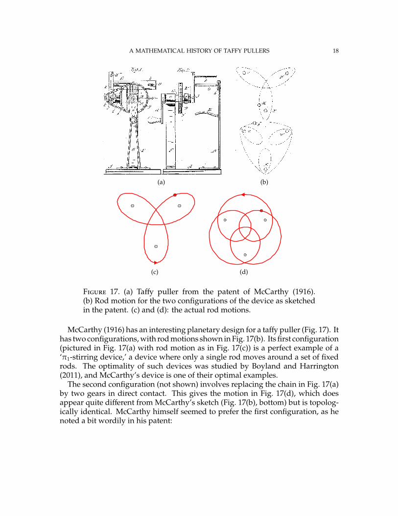
Figure 17. (a) Taffy puller from the patent of McCarthy (1916).(b) Rod motion for the two configurations of the device as sketchedin the patent. (c) and (d): the actual rod motions.

McCarthy (1916) has an interesting planetary design for a taffy puller (Fig. 17). Ithas two configurations, with rod motions shown in Fig. 17(b). Its first configuration(pictured in Fig. 17(a) with rod motion as in Fig. 17(c)) is a perfect example of a‘π1-stirring device,’ a device where only a single rod moves around a set of fixedrods. The optimality of such devices was studied by Boyland and Harrington(2011), and McCarthy’s device is one of their optimal examples.

The second configuration (not shown) involves replacing the chain in Fig. 17(a)by two gears in direct contact. This gives the motion in Fig. 17(d), which doesappear quite different from McCarthy’s sketch (Fig. 17(b), bottom) but is topolog-ically identical. McCarthy himself seemed to prefer the first configuration, as henoted a bit wordily in his patent:


The planetary course described by this pin, when this modifiedconstruction is employed, gives a constant pull to the candy, butdoes not accomplish as thorough mixing of the same as when saidpin describes the planetary course resulting from the construction ofthe preferred form of my invention, as hereinbefore first described.

What he meant by ‘a constant pull to the candy’ is probably that in the secondconfiguration the rod moves back and forth in the center of the device, so thetaffy would sometimes be unstretched. In the first configuration the rod resolutelytraverses the center of the device in a single direction each time, leading to uniformstretching. As far as the less thorough mixing he mentions is concerned, in oneturn of the handle the first configuration gives a dilatation of 4.2361, while thesecond has 2.4229. However, the second design has a larger dilatation for a fullperiod of the rod motion, as given in Table 1. This illustrates the difficultiesinvolved in comparing the efficiency of different devices, which we will return toin Section 5. In its first configuration the device has a quadratic dilatation, thelargest root of x2

− 18x + 1. In its second configuration the dilatation is a quarticnumber, the largest root of x4

− 36x3 + 5x2− 36x + 1.

Another planetary device, the mixograph, is shown in Fig. 18. The mixographconsists of a small cylindrical vessel with three fixed vertical rods. A lid is loweredonto the base. The lid has two gears each with a pair of rods, and is itself rotating,resulting in a net complex ‘spirograph’ motion as in Fig. 18(c) (top). The mixographis used to measure properties of bread dough: a piece of dough is placed in thedevice, and the torque on the rods is recorded on graph paper (in a similar mannerto a seismograph). An expert on bread dough can then deduce dough-mixingcharacteristics from the graph (Connelly and Valenti-Jordan 2008).

Clearly, passing to a uniformly-rotating frame does not modify the dilatation.For the mixograph, a frame where the fixed rods rotate simplifies the orbits some-what (Fig. 18(c), bottom). This has another advantage: in this ‘co-rotating’ picture,the rods return to their initial configuration (as a set) much sooner than in the fixedpicture. This makes the map simpler, and we then take a power of this co-rotatingmap to recover the original. The rod motion of Fig. 18(c) (bottom) must be re-peated six times for all the rods to return to their initial position. The dilatationfor the co-rotating map is the largest root of x8

− 4x7− x6 + 4x4

− x2− 4x + 1, which

is approximately 4.1858.

4.2. A few more designs. The design of Jenner (1905), shown in Fig. 19, is a fairlystraightforward variant of the other devices we’ve seen. From our point of viewit has a peculiar property: its dilatation is the largest root of the polynomial x4

−

8x3− 2x2

− 8x + 1, which is the strange number (ϕ +√ϕ)2, where ϕ is the Golden

Ratio.


(a)(b)

(c)

Figure 18. (a) The mixograph, a planetary rod mixer for breaddough. (b) Top section with four moving rods (above), and bot-tom section with three fixed rods (below). (c) The rod motion iscomplex (top), but is less so in a rotating frame (bottom). (Courtesyof the Department of Food Science, University of Wisconsin. Photoby the author, from Finn and Thiffeault (2011).)

The taffy puller of Shean and Schmelz (1914) is shown in Fig. 20. The design issomewhat novel, since it is not based directly on gears. It consists of two inter-locking ‘combs’ of three rods each, for a total of six moving rods. Mathematically,this device has exactly the same dilatation as the earlier 6-rod design (Fig. 12). Asimilar comb design was later used in a device for homogenizing molten glass(Russell and Wiley 1951).

We finish with the intriguing design of McCarthy and Wilson (1915), shown inFig. 21. This is the most baroque design we’ve encountered: it contains a recipro-cating arm, rotating rods, and fixed rods. The inventors did seem to know whatthey were doing with this complexity: its dilatation is enormous at approximately21.2667, the largest root of x4

− 20x3− 26x2

− 20x + 1.

5. Discussion

The reader might be wondering at this point: which is the best taffy puller inhistory? Did all these incremental changes and new designs lead to measurableprogress in the effectiveness of taffy pullers? Table 1 collects the characteristic


(a) (b)

Figure 19. Taffy puller from the patent of Jenner (1905). (b) Themotion of the rods, with three fixed rods in gray.

(a) (b)

Figure 20. (a) Taffy puller from the patent of Shean and Schmelz(1914). (b) The rod motion.

polynomials and the dilatations (the largest root) for all the taffy pullers discussedhere. The total number of rods is listed (the number in parentheses is the numberof fixed rods).

The column labeled p requires a bit of explanation. Comparing the differenttaffy pullers is not straightforward. For example, for the first mode of operationof the device by McCarthy (1916), in Fig. 17(c), two full turns of the crank arerequired for the rod to come back to its initial position. For the second mode, in


(a) (b)

Figure 21. (a) Taffy puller from the patent of McCarthy and Wilson(1915). (b) Rod motion.

Fig. 17(d), four turns are required. The second mode has a larger dilatation, butit clearly requires more work. A full characterization of the efficiency of a taffypuller would have to take into account the torque required to pull the candy.

To keep things simple, we define the efficiency in terms of the total dilatationfor a full period, where a full period is defined by all the rods returning to theirinitial positions. For example, referring to Table 1, for the Thibodeau 1904 devicethe rods return to the same configuration as a set after p = 1/3 of a period. Hence,the dilatation listed, ϕ2 is for 1/3 of a period. We define its efficiency as theentropy (logarithm of the dilatation) per period. Hence, in this case the efficiencyis log(ϕ2)/(1/3) = 6 logϕ ≈ 2.8873.

By this measure, the mixograph is the clear winner, with a staggering efficiencyof 8.5902. Of course, it also has the most rods. The large efficiency is mostly dueto how long the rods take to return to their initial position.

Some observations can be made regarding the taffy pullers presented. Witha few exceptions, they all give pseudo-Anosov maps. The inventors were thusaware, at least intuitively, that there should be no unnecessary rods.

Another observation is that most of the dilatations are quadratic numbers. Thereare probably a few reasons for this. One is that the polynomial giving the dilatationexpresses a recurrence relation that characterizes how the folds are combined ateach period. With a small number, of rods, there is a limit to the degree of


Table 1. Efficiency of taffy pullers. A number of rods such as 6 (2)indicates 6 total rods, with 2 fixed. The largest root of the polynomialis the dilatation. The dilatation corresponds to a fraction p of a fullperiod, when each rod returns to its initial position. The entropyper period is log(dilatation)/period, which is a crude measure ofefficiency. Here ϕ = 1

2 (1 +√

5) is the Golden Ratio, and χ = 1 +√

2is the Silver Ratio.

puller fig. rods polynomial dilatation pentropy/period

standard 3-rod 3 3 (1) x2− 6x + 1 χ2 1 1.7627

Nitz (1918) 4 3 x2− 3x + 1 ϕ2 1/3 2.8873

standard 4-rod 8 4 x2− 6x + 1 χ2 1 1.7627

Thibodeau (1904) 11 4 x2− 3x + 1 ϕ2 1/3 2.8873

6-rod 12 6 (2) x2− 4x + 1 2 +

√3 1/2 2.6339

McCarthy (1916) † 17(c) 4 (3) x2− 18x + 1 ϕ6 1 2.8873

17(d) 4 (3) x4− 36x3 + 5x2

− 36x + 1 34.4634 1 3.5399

mixograph ‡ 18(c) 7x8− 4x7

− x6 + 4x4

− x2− 4x + 1 4.1858 1/6 8.5902

Jenner (1905) 19 5 (3) x4− 8x3

− 2x2− 8x + 1 (ϕ +

√ϕ)2 1 2.1226

Shean (1914) 20 6 x2− 4x + 1 2 +

√3 1/2 2.6339

McCarthy (1915) 21 5 (2) x4− 20x3

− 26x2− 20x + 1 21.2667 1 3.0571

† The McCarthy (1916) device has two configurations.‡ This is the co-rotating version of the mixograph (Fig. 18(c), bottom).

this recurrence (2n − 4 for n rods). A second reason is that more rods does notnecessarily mean larger dilatation (Finn and Thiffeault 2011). On the contrary, morerods allows for a smaller dilatation, as observed when finding the smallest valueof the dilatation (Hironaka and Kin 2006; Lanneau and Thiffeault 2011; Thiffeaultand Finn 2006; Venzke 2008).

The collection of taffy pullers presented here can be thought of as a battery ofexamples to illustrate various types of pseudo-Anosov maps. Even though theydid not come out of the mathematical literature, they predate by many decades theexamples that were later constructed by many groups (Binder 2010; Binder andCox 2008; Boyland, Aref, and Stremler 2000; Boyland and Harrington 2011; Finnand Thiffeault 2011; Kobayashi and Umeda 2007, 2010; Thiffeault and Finn 2006).

There are actually quite a few more patents for taffy pullers that were not shownhere (only U.S. patents were searched). An obvious question is: why so many?Often the answer is that a new patent is created to get around an earlier one,but the very first patents had lapsed by the 1920s and yet more designs were

REFERENCES 24

introduced, so this is only a partial answer. Perhaps there is a natural responsewhen looking at a taffy puller to think that we can design a better one, since thebasic idea is so simple. At least mathematics provides a way of making sure thatwe’ve thoroughly explored all designs, and to gauge the effectiveness of existingones.

References

Binder, B. J. (2010). “Ghost rods adopting the role of withdrawn baffles in batchmixer designs.” Phys. Lett. A 374, 3483–3486.

Binder, B. J. and S. M. Cox (2008). “A mixer design for the pigtail braid.” Fluid Dyn.Res. 40, 34–44.

Boyland, P. L., H. Aref, and M. A. Stremler (2000). “Topological fluid mechanics ofstirring.” J. Fluid Mech. 403, 277–304.

Boyland, P. L. and J. Harrington (2011). “The entropy efficiency of point-pushmapping classes on the punctured disk.” Algeb. Geom. Topology 11(4), 2265–2296.

Connelly, R. K. and J. Valenti-Jordan (Dec. 2008). “Mixing analysis of a Newtonianfluid in a 3D planetary pin mixer.” 86(12), 1434–1440.

Dickinson, H. M. (Sept. 1906). “Candy-pulling machine.” Pat. US831501 A.Farb, B. and D. Margalit (2011). A Primer on Mapping Class Groups. Princeton, NJ:

Princeton University Press.Fathi, A., F. Laundenbach, and V. Poénaru (1979). “Travaux de Thurston sur les

surfaces.” Astérisque 66-67, 1–284.Finn, M. D. and J.-L. Thiffeault (Dec. 2011). “Topological optimization of rod-

stirring devices.” SIAM Rev. 53(4), 723–743.Firchau, P. J. G. (Dec. 1893). “Machine for working candy.” Pat. US511011 A.Franks, J. and E. Rykken (1999). “Pseudo-Anosov homeomorphisms with qua-

dratic expansion.” Proc. Amer. Math. Soc. 127, 2183–2192.Halbert, J. T. and J. A. Yorke (2014). “Modeling a chaotic machine’s dynamics as a

linear map on a “square sphere”.” Topology Proceedings 44, 257–284.Hall, T. (2012). Train: A C++ program for computing train tracks of surface homeomor-

phisms. http://www.liv.ac.uk/~tobyhall/T_Hall.html.Hironaka, E. and E. Kin (2006). “A family of pseudo-Anosov braids with small

dilatation.” Algebraic & Geometric Topology 6, 699–738.Hudson, W. T. (Feb. 1904). “Candy-working machine.” Pat. US752226 A.Jenner, E. J. (Nov. 1905). “Candy-pulling machine.” Pat. US804726 A.Kirsch, E. (Jan. 1928). “Candy-pulling machine.” Pat. US1656005 A.

http://www.liv.ac.uk/~tobyhall/T_Hall.html

REFERENCES 25

Kobayashi, T. and S. Umeda (2007). “Realizing pseudo-Anosov egg beaters withsimple mecanisms.” In: Proceedings of the International Workshop on Knot Theoryfor Scientific Objects, Osaka, Japan. Osaka, Japan: Osaka Municipal UniversitiesPress, pp. 97–109.

– (2010). “A design for pseudo-Anosov braids using hypotrochoid curves.” Topol-ogy Appl. 157, 280–289.

Lanneau, E. and J.-L. Thiffeault (June 2011). “On the minimum dilatation of braidson the punctured disc.” Geometriae Dedicata 152(1), 165–182.

MacKay, R. S. (2001). “Complicated dynamics from simple topological hypothe-ses.” Phil. Trans. R. Soc. Lond. A 359, 1479–1496.

McCarthy, E. F. (May 1916). “Candy-pulling machine.” Pat. US1182394 A.McCarthy, E. F. and E. W. Wilson (May 1915). “Candy-pulling machine.” Pat.

US1139786 A.Nitz, C. G. W. (Sept. 1918). “Candy-puller.” Pat. US1278197 A.Richards, F. H. (May 1905). “Process of making candy.” Pat. US790920 A.Robinson, E. M. and J. H. Deiter (Mar. 1908). “Candy-pulling machine.” Pat.

US881442 A.Russell, R. G. and R. B. Wiley (Dec. 1951). “Apparatus for mixing viscous liquids.”

Pat. US2577920 A.Shean, G. C. C. and L. Schmelz (Oct. 1914). “Candy-pulling machine.” Pat. US1112569 A.Thibodeau, C. (Aug. 1903). “Method of pulling candy.” Pat. US736313 A.– (Oct. 1904). “Candy-pulling machine.” Pat. US772442 A.Thiffeault, J.-L. and M. D. Finn (Dec. 2006). “Topology, braids, and mixing in

fluids.” Phil. Trans. R. Soc. Lond. A 364, 3251–3266.Thiffeault, J.-L. and M. Budišic (2013–2016). Braidlab: A Software Package for Braids

and Loops. http://arXiv.org/abs/1410.0849, Version 3.2.Thurston, W. P. (1988). “On the geometry and dynamics of diffeomorphisms of

surfaces.” Bull. Am. Math. Soc. 19, 417–431.Venzke, R. W. (2008). Braid Forcing, Hyperbolic Geometry, and Pseudo-Anosov Se-

quences of Low Entropy. PhD thesis. California Institute of Technology.Zorich, A. (2006). “Flat surfaces.” In: Frontiers in Number Theory, Physics, and Geom-

etry. Ed. by P. Cartier et al. Vol. 1. Berlin: Springer, pp. 439–586.

Department ofMathematics, University ofWisconsin, Madison, WI 53706, USAE-mail address: [email protected]

http://arXiv.org/abs/1410.0849

a mathematical history of taffy pullersa mathematical history of taffy pullers 2 2. some history the...

Documents