The elastica: a mathematical history

Raph Levien

Electrical Engineering and Computer SciencesUniversity of California at Berkeley

Technical Report No. UCB/EECS-2008-103

http://www.eecs.berkeley.edu/Pubs/TechRpts/2008/EECS-2008-103.html

August 23, 2008

Copyright 2008, by the author(s).All rights reserved.

Permission to make digital or hard copies of all or part of this work forpersonal or classroom use is granted without fee provided that copies arenot made or distributed for profit or commercial advantage and that copiesbear this notice and the full citation on the first page. To copy otherwise, torepublish, to post on servers or to redistribute to lists, requires prior specificpermission.

The elastica: a mathematical history

Raph Levien

August 23, 2008

Abstract

This report traces the history of the elastica from its first precise formulation by James Bernoulli in1691 through the present. The complete solution is most commonly attributed to Euler in 1744 becauseof his compelling mathematical treatment and illustrations, but in fact James Bernoulli had arrived atthe correct equation a half-century earlier. The elastica can be understood from a number of differentaspects, including as a mechanical equilibrium, a problem of the calculus of variations, and the solutionto elliptic integrals. In addition, it has a number of analogies with physical systems, including a sheetholding a volume of water, the surface of a capillary, and the motion of a simple pendulum. It is alsothe mathematical model of the mechanical spline, used for shipbuilding and similar applications, anddirectly insipired the modern theory of mathematical splines. More recently, the major focus has beenon efficient numerical techniques for computing the elastica and fitting it to spline problems. All in all,it is a beautiful family of curves based on beautiful mathematics and a rich and fascinating history.

This report is adapted from a Ph. D. thesis done under the direction of Prof. C. H. Sequin.

1 Introduction

This report tells the story of a remarkable family of curves, known as the elastica, Latin for a thin stripof elastic material. The elastica caught the attention of many of the brightest minds in the history ofmathematics, including Galileo, the Bernoullis, Euler, and others. It was present at the birth of manyimportant fields, most notably the theory of elasticity, the calculus of variations, and the theory ofelliptic integrals. The path traced by this curve illuminates a wide range of mathematical style, from themechanics-based intuition of the early work, through a period of technical virtuosity in mathematicaltechnique, to the present day where computational techniques dominate.

There are many approaches to the elastica. The earliest (and most mathematically tractable), is asan equilibrium of moments, drawing on a fundamental principle of statics. Another approach, ultimatelyyielding the same equation for the curve, is as a minimum of bending energy in the elastic curve. A force-based approach finds that normal, compression, and shear forces are also in equilibrium; this approachis useful when considering specific constraints on the endpoints, which are often intuitively expressed interms of these forces.

Later, the fundamental differential equation for the elastica was found to be equivalent to that for themotion of the simple pendulum. This formulation is most useful for appreciating the curve’s periodicity,and also helps understand special values in the parameter space.

In more recent times, the focus has been on efficient numerical computation of the elastica (especiallyfor the application of fitting smooth spline curves through a sequence of points), and also determining therange of endpoint conditions for which a stable solution exists. Many practical applications continue touse brute-force numerical techniques, but in many cases the insights of mathematicians (many workinghundreds of years earlier) still have power to inspire a more refined computational approach.

2 Jordanus de Nemore—13th century

In the recorded literature, the problem of the elastica was first posed in De Ratione Ponderis by Jordanusde Nemore (Jordan of the Forest), a thirteenth century mathematician. Proposition 13 of book 4 states

1

that “when the middle is held fast, the end parts are more easily curved.” He then poses an incorrectsolution: “And so it comes about that since the ends yield most easily, while the other parts follow moreeasily to the extent that they are nearer the ends, the whole body becomes curved in a circle.” [8]. Infact, the circle is one possible solution to the elastica, but not to not for the specific problem posed. Evenso, this is a clear statement of the problem, and the solution (though not correct) is given in the form ofa specific mathematical curve. It would be several centuries until the mathematical concepts needed toanswer the question came into existence.

3 Galilieo sets the stage—1638

Three basic concepts are required for the formulation of the elastica as an equilibrium of moments:moment (a fundamental principle of statics), the curvature of a curve, and the relationship betweenthese two concepts. In the case of an idealized elastic strip, these quantities are linearly related.

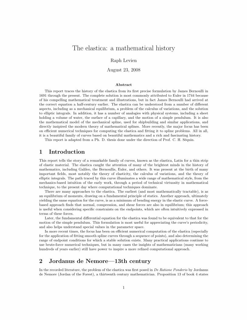
Figure 1: Galileo’s 1638 problem.

Galileo, in 1638, posed a fundamental problem, founding the mathematical study of elasticity. Givena prismatic beam set into a wall at one end, and loaded by a weight at the other, how much weight isrequired to break the beam? The delightful Figure 1 illustrates the setup. Galileo considers the beamto be a compound lever with a fulcrum at the bottom of the beam meeting the wall at B. The weight Eacts on one arm BC, and the thickness of the beam at the wall, AB, is the other arm, “in which residesthe resistance.” His first proposition is, “The moment of force at C to the moment of the resistance...has the same propotion as the length CB to the half of BA, and therefore the absolute resistance tobreaking... is to the resistance in the same proportion as the length of BC to the half of AB...”

From these basic principles, Galileo derives a number of results, primarily a scaling relationship.He does not consider displacements of the beam; for these types of structural beams, the displacementis neglible. Even so, this represents the first mathematical treatment of a problem in elasticity, andfirmly establishes the concept of moment to determine the force on an elastic material. Many researcherselaborated on Galileo’s results in coming decades, as described in detail in Todhunder’s history [33].

2

One such researcher is Ignace-Gaston Pardies, who in 1673 posed one form of the elastica problemand also attempts a solution: for a beam held fixed at one end and loaded by a weight at the other, “it iseasy to prove” that it is a parabola. However, this solution isn’t even approximately correct, and wouldlater be dismissed by James Bernoulli as one of several “pure fallacies.” Truesdell gives Pardies creditfor introducing the elasticity of a beam into calculation of its resistance, and traces out his influence onsubsequent researchers, particularly Leibniz and James Bernoulli [34, p. 50–53].

4 Hooke’s law of the spring—1678

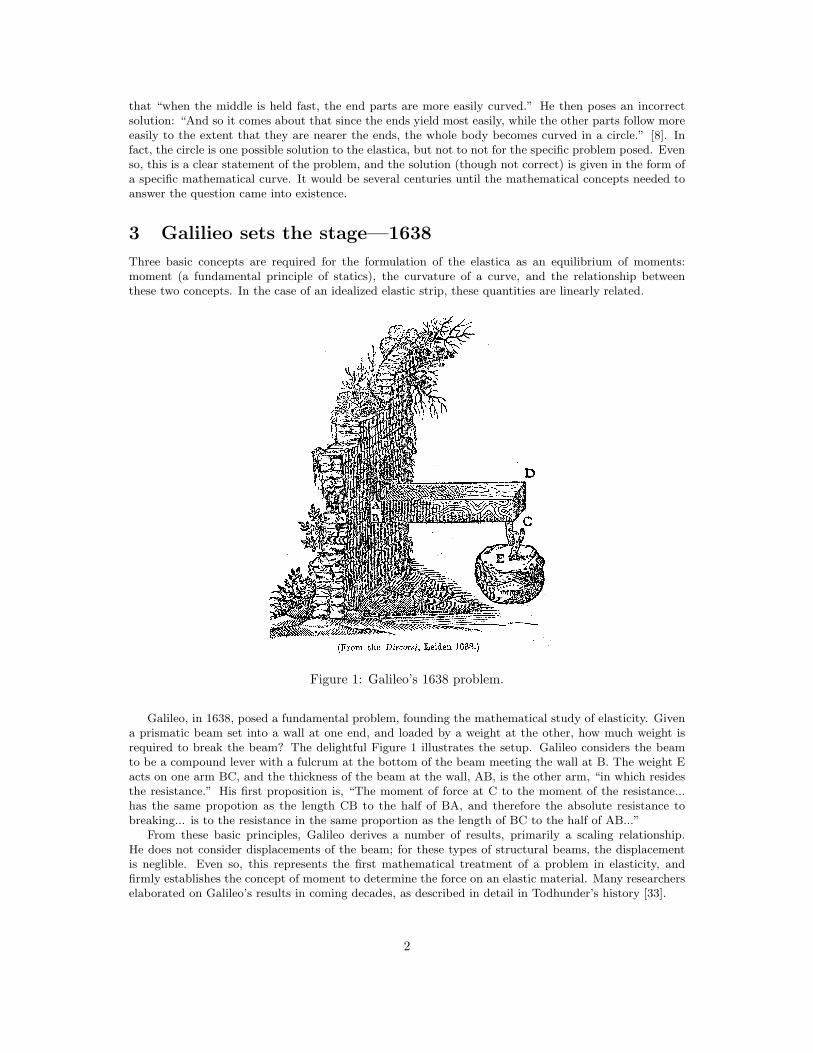
Hooke published a treatise on elasticity in 1678, containing his famous law. In a short Latin phraseposed in a cryptic anagram three years earlier to establish priority, it reads, “ut tensio sic vis; that is,The Power of any Spring is in the same proportion with the Tension thereof... Now as the Theory isvery short, so the way of trying it is very easie.” (spelling and capitalization as in original). In modernformulation, it is understood as F ∝ ∆l; the applied force is proportional to the change in length.

Figure 2: Hooke’s figure on compound elasticity.

Hooke touches on the problem of elastic strips, providing an evocative illustration (Figure 2), butaccording to Truesdell, “This ‘compound way of springing’ is the main problem of elasticity for thecentury following, but Hooke gives no idea how to relate the curvature of one fibre to the bendingmoment, not to mention the reaction of the two fibres on one another.” [34, p. 55]

Indeed, mathematical understanding of curvature was still in development at the time, and masteryover it would have to wait for the calculus. Newton published results on curvature in his “Methods ofSeries and Fluxions,” written 1670 to 1671 [17, p. 232], but not published for several more years. Leibnizsimilarly used his competing version of the calculus to derive similar results. Even so, some resultswere possible with pre-calculus methods, and in 1673, Christiaan Huygens published the “Horologiumoscillatorium sive de motu pendulorum ad horologia aptato demonstrationes geometrica,” which usedpurely geometric constructions, particularly the involutes and evolutes of curves, to establish resultsinvolving curvature. The flavor of geometric construction pervades much of the early work on elasticity,particularly James Bernoulli’s, as we shall see.

Newton also used his version of the calculus to more deeply understand curvature, and provided theformulation for radius of curvature in terms of Cartesian coordinates most familiar to us today [17]:

ρ = (1 + y′2)32 /y′′ (1)

An accessible introduction to the history of curvature is the aptly named “History of Curvature” byDan Margalit [24].

Given a solid mathematical understanding of curvature, and assuming a linear relation between forceand change of length, working out the relationship between moment and curvature is indeed “easie,” buteven Bernoulli had to struggle a bit with both concepts. For one, Bernoulli didn’t simply accept thelinear law of the spring, but felt the need to test it for himself. And, since he had the misfortune touse catgut, rather than a more ideally elastic material such as metal, he found significant nonlinearities.Truesdell [36] recounts a letter from James Bernoulli to Leibniz on 15 December 1687, and the replyof Leibniz almost three years later. According to Truesdell, this exchange is the birth of the theory

3

of the “curva elastica” and its ramifications. Leibniz had proposed: “From the hypothesis elsewheresubstantiated, that the extensions are proportional to the stretching forces...” which is today attributedas Hooke’s law of the spring. Bernoulli questioned this relationship, and, as we shall see, his solution tothe elastica generalized even to nonlinear displacement.

5 James Bernoulli poses the elastica problem—1691

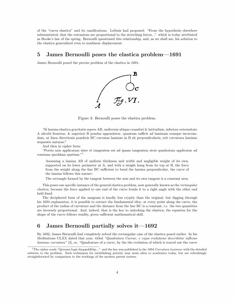
James Bernoulli posed the precise problem of the elastica in 1691:

Figure 3: Bernoulli poses the elastica problem.

“Si lamina elastica gravitatis espers AB, uniformis ubique crassitiei & latitudinis, inferiore extremitateA alicubi firmetur, & superiori B pondus appendatur, quantum sufficit ad laminam eousque incurvan-dam, ut linea directionis ponderis BC curvatae laminae in B sit perpendicularis, erit curvatura laminaesequentis naturae:”

And then in cipher form:“Portio axis applicatam inter et tangentem est ad ipsam tangentem sicut quadratum applicatae ad

constans quoddam spatium.”1

Assuming a lamina AB of uniform thickness and width and negligible weight of its own,supported on its lower perimeter at A, and with a weight hung from its top at B, the forcefrom the weight along the line BC sufficient to bend the lamina perpendicular, the curve ofthe lamina follows this nature:

The rectangle formed by the tangent between the axis and its own tangent is a constant area.

This poses one specific instance of the general elastica problem, now generally known as the rectangularelastica, because the force applied to one end of the curve bends it to a right angle with the other endheld fixed.

The deciphered form of the anagram is hardly less cryptic than the original, but digging throughhis 1694 explanation, it is possible to extract the fundamental idea: at every point along the curve, theproduct of the radius of curvature and the distance from the line BC is a constant, i.e. the two quantitiesare inversely proportional. And, indeed, that is the key to unlocking the elastica; the equation for theshape of the curve follows readily, given sufficient mathematical skill.

6 James Bernoulli partially solves it—1692

By 1692, James Bernoulli had completely solved the rectangular case of the elastica posed earlier. In hisMeditatione CLXX dated that year, titled “Quadratura Curvae, e cujus evolutione describitur inflexaelaminae curvatura” [3], or, “Quadrature of a curve, by the the evolution of which is traced out the curve

1The cipher reads “Qrzumu bapt dxqopddbbp...” and the key was published in the 1694 Curvatura Laminae with the detailedsolution to the problem. Such techniques for establishing priority may seem alien to academics today, but are refreshinglystraightforward by comparison to the workings of the modern patent system.

4

A

B

C

D

E F

G H

IL

M N

Q

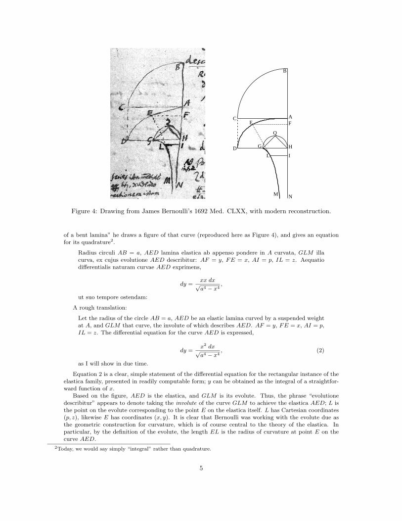
Figure 4: Drawing from James Bernoulli’s 1692 Med. CLXX, with modern reconstruction.

of a bent lamina” he draws a figure of that curve (reproduced here as Figure 4), and gives an equationfor its quadrature2.

Radius circuli AB = a, AED lamina elastica ab appenso pondere in A curvata, GLM illacurva, ex cujus evolutione AED describitur: AF = y, FE = x, AI = p, IL = z. Aequatiodifferentialis naturam curvae AED exprimens,

dy =xx dx√a4 − x4

,

ut suo tempore ostendam:

A rough translation:

Let the radius of the circle AB = a, AED be an elastic lamina curved by a suspended weightat A, and GLM that curve, the involute of which describes AED. AF = y, FE = x, AI = p,IL = z. The differential equation for the curve AED is expressed,

dy =x2 dx√a4 − x4

, (2)

as I will show in due time.

Equation 2 is a clear, simple statement of the differential equation for the rectangular instance of theelastica family, presented in readily computable form; y can be obtained as the integral of a straightfor-ward function of x.

Based on the figure, AED is the elastica, and GLM is its evolute. Thus, the phrase “evolutionedescribitur” appears to denote taking the involute of the curve GLM to achieve the elastica AED; L isthe point on the evolute corresponding to the point E on the elastica itself. L has Cartesian coordinates(p, z), likewise E has coordinates (x, y). It is clear that Bernoulli was working with the evolute due asthe geometric construction for curvature, which is of course central to the theory of the elastica. Inparticular, by the definition of the evolute, the length EL is the radius of curvature at point E on thecurve AED.

2Today, we would say simply “integral” rather than quadrature.

5

7 James Bernoulli publishes the first solution—1694

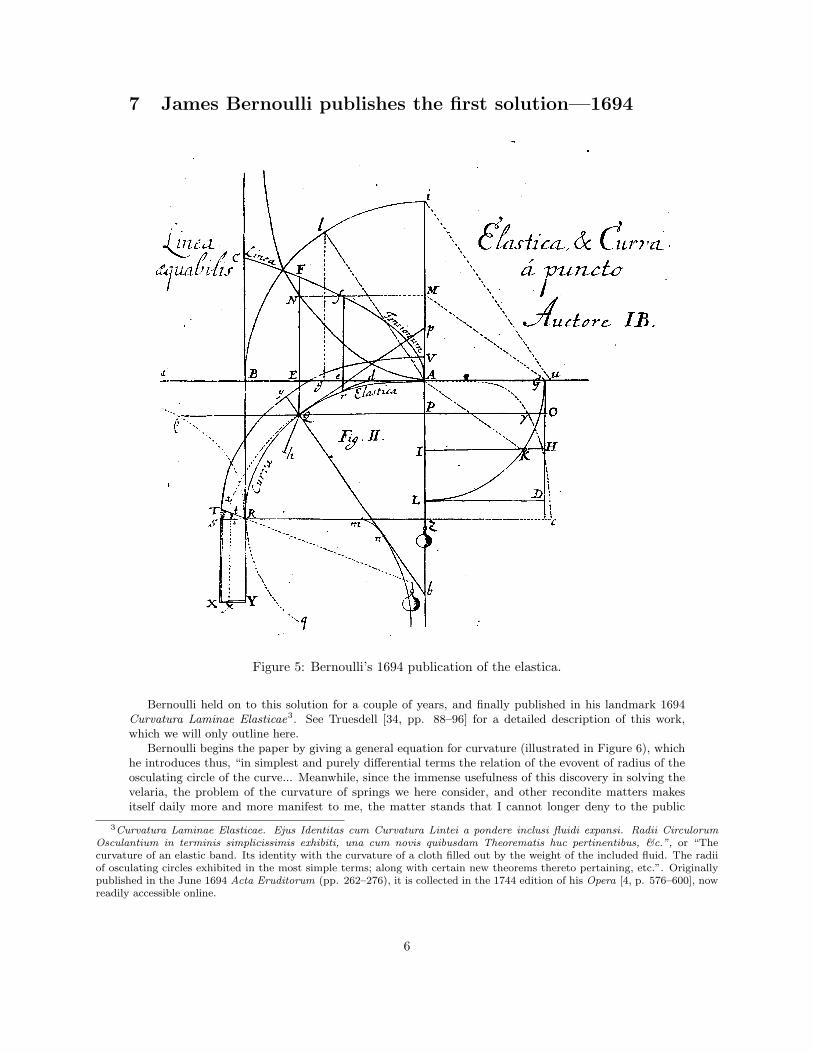
Figure 5: Bernoulli’s 1694 publication of the elastica.

Bernoulli held on to this solution for a couple of years, and finally published in his landmark 1694Curvatura Laminae Elasticae3. See Truesdell [34, pp. 88–96] for a detailed description of this work,which we will only outline here.

Bernoulli begins the paper by giving a general equation for curvature (illustrated in Figure 6), whichhe introduces thus, “in simplest and purely differential terms the relation of the evovent of radius of theosculating circle of the curve... Meanwhile, since the immense usefulness of this discovery in solving thevelaria, the problem of the curvature of springs we here consider, and other recondite matters makesitself daily more and more manifest to me, the matter stands that I cannot longer deny to the public

3Curvatura Laminae Elasticae. Ejus Identitas cum Curvatura Lintei a pondere inclusi fluidi expansi. Radii CirculorumOsculantium in terminis simplicissimis exhibiti, una cum novis quibusdam Theorematis huc pertinentibus, &c.”, or “Thecurvature of an elastic band. Its identity with the curvature of a cloth filled out by the weight of the included fluid. The radiiof osculating circles exhibited in the most simple terms; along with certain new theorems thereto pertaining, etc.”. Originallypublished in the June 1694 Acta Eruditorum (pp. 262–276), it is collected in the 1744 edition of his Opera [4, p. 576–600], nowreadily accessible online.

6

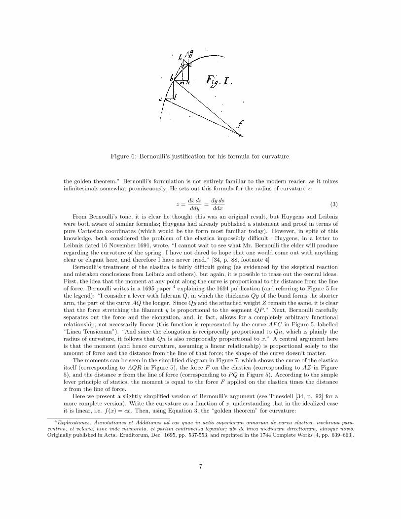
Figure 6: Bernoulli’s justification for his formula for curvature.

the golden theorem.” Bernoulli’s formulation is not entirely familiar to the modern reader, as it mixesinfinitesimals somewhat promiscuously. He sets out this formula for the radius of curvature z:

z =dx ds

ddy=

dy ds

ddx(3)

From Bernoulli’s tone, it is clear he thought this was an original result, but Huygens and Leibnizwere both aware of similar formulas; Huygens had already published a statement and proof in terms ofpure Cartesian coordinates (which would be the form most familiar today). However, in spite of thisknowledge, both considered the problem of the elastica impossibly difficult. Huygens, in a letter toLeibniz dated 16 November 1691, wrote, “I cannot wait to see what Mr. Bernoulli the elder will produceregarding the curvature of the spring. I have not dared to hope that one would come out with anythingclear or elegant here, and therefore I have never tried.” [34, p. 88, footnote 4]

Bernoulli’s treatment of the elastica is fairly difficult going (as evidenced by the skeptical reactionand mistaken conclusions from Leibniz and others), but again, it is possible to tease out the central ideas.First, the idea that the moment at any point along the curve is proportional to the distance from the lineof force. Bernoulli writes in a 1695 paper 4 explaining the 1694 publication (and referring to Figure 5 forthe legend): “I consider a lever with fulcrum Q, in which the thickness Qy of the band forms the shorterarm, the part of the curve AQ the longer. Since Qy and the attached weight Z remain the same, it is clearthat the force stretching the filament y is proportional to the segment QP .” Next, Bernoulli carefullyseparates out the force and the elongation, and, in fact, allows for a completely arbitrary functionalrelationship, not necessarily linear (this function is represented by the curve AFC in Figure 5, labelled“Linea Tensionum”). “And since the elongation is reciprocally proportional to Qn, which is plainly theradius of curvature, it follows that Qn is also reciprocally proportional to x.” A central argument hereis that the moment (and hence curvature, assuming a linear relationship) is proportional solely to theamount of force and the distance from the line of that force; the shape of the curve doesn’t matter.

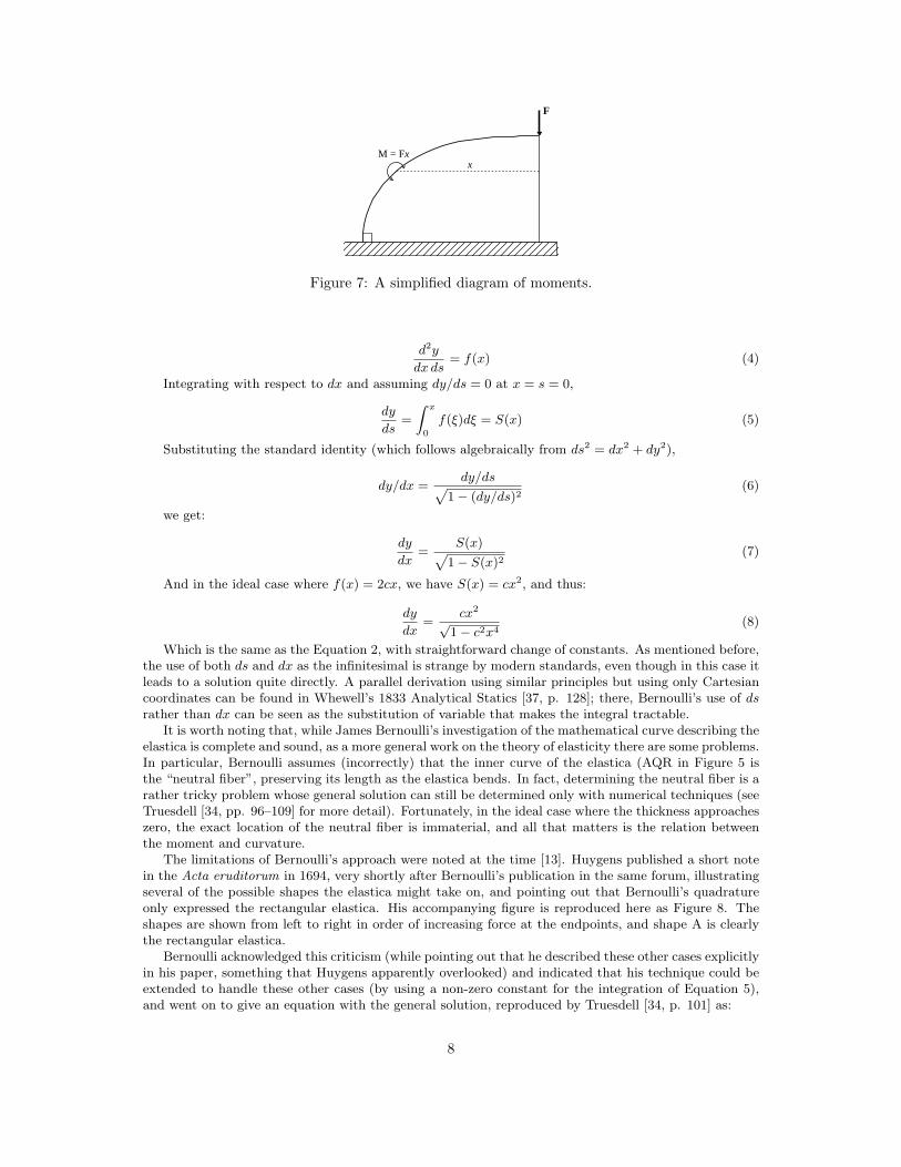
The moments can be seen in the simplified diagram in Figure 7, which shows the curve of the elasticaitself (corresponding to AQR in Figure 5), the force F on the elastica (corresponding to AZ in Figure5), and the distance x from the line of force (corresponding to PQ in Figure 5). According to the simplelever principle of statics, the moment is equal to the force F applied on the elastica times the distancex from the line of force.

Here we present a slightly simplified version of Bernoulli’s argument (see Truesdell [34, p. 92] for amore complete version). Write the curvature as a function of x, understanding that in the idealized caseit is linear, i.e. f(x) = cx. Then, using Equation 3, the “golden theorem” for curvature:

4Explicationes, Annotationes et Additiones ad eas quae in actis superiorum annorum de curva elastica, isochrona para-centrua, et velaria, hinc inde memorata, et partim controversa leguntur; ubi de linea mediarum directionum, aliisque novis.Originally published in Acta. Eruditorum, Dec. 1695, pp. 537-553, and reprinted in the 1744 Complete Works [4, pp. 639–663].

7

F

xM = Fx

Figure 7: A simplified diagram of moments.

d2y

dx ds= f(x) (4)

Integrating with respect to dx and assuming dy/ds = 0 at x = s = 0,

dy

ds=

Z x

0

f(ξ)dξ = S(x) (5)

Substituting the standard identity (which follows algebraically from ds2 = dx2 + dy2),

dy/dx =dy/dsp

1− (dy/ds)2(6)

we get:

dy

dx=

S(x)p1− S(x)2

(7)

And in the ideal case where f(x) = 2cx, we have S(x) = cx2, and thus:

dy

dx=

cx2

√1− c2x4

(8)

Which is the same as the Equation 2, with straightforward change of constants. As mentioned before,the use of both ds and dx as the infinitesimal is strange by modern standards, even though in this case itleads to a solution quite directly. A parallel derivation using similar principles but using only Cartesiancoordinates can be found in Whewell’s 1833 Analytical Statics [37, p. 128]; there, Bernoulli’s use of dsrather than dx can be seen as the substitution of variable that makes the integral tractable.

It is worth noting that, while James Bernoulli’s investigation of the mathematical curve describing theelastica is complete and sound, as a more general work on the theory of elasticity there are some problems.In particular, Bernoulli assumes (incorrectly) that the inner curve of the elastica (AQR in Figure 5 isthe “neutral fiber”, preserving its length as the elastica bends. In fact, determining the neutral fiber is arather tricky problem whose general solution can still be determined only with numerical techniques (seeTruesdell [34, pp. 96–109] for more detail). Fortunately, in the ideal case where the thickness approacheszero, the exact location of the neutral fiber is immaterial, and all that matters is the relation betweenthe moment and curvature.

The limitations of Bernoulli’s approach were noted at the time [13]. Huygens published a short notein the Acta eruditorum in 1694, very shortly after Bernoulli’s publication in the same forum, illustratingseveral of the possible shapes the elastica might take on, and pointing out that Bernoulli’s quadratureonly expressed the rectangular elastica. His accompanying figure is reproduced here as Figure 8. Theshapes are shown from left to right in order of increasing force at the endpoints, and shape A is clearlythe rectangular elastica.

Bernoulli acknowledged this criticism (while pointing out that he described these other cases explicitlyin his paper, something that Huygens apparently overlooked) and indicated that his technique could beextended to handle these other cases (by using a non-zero constant for the integration of Equation 5),and went on to give an equation with the general solution, reproduced by Truesdell [34, p. 101] as:

8

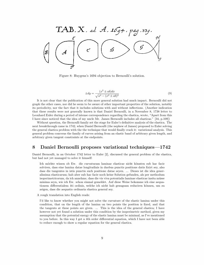
Figure 8: Huygens’s 1694 objection to Bernoulli’s solution.

±dy =(x2 ± ab)dxpa4 − (x2 ± ab)2

(9)

It is not clear that the publication of this more general solution had much impact. Bernoulli did notgraph the other cases, nor did he seem to be aware of other important properties of the solution, notablyits periodicity, nor the fact that it includes solutions with and without inflections. (Another indicationthat these results were not generally known is that Daniel Bernoulli, in a November 8, 1738 letter toLeonhard Euler during a period of intense correspondence regarding the elastica, wrote, “Apart from thisI have since noticed that the idea of my uncle Mr. James Bernoulli includes all elasticas.” [34, p.109])

Without question, the Bernoulli family set the stage for Euler’s definitive analysis of the elastica. Thenext breakthrough came in 1742, when Daniel Bernoulli (the nephew of James) proposed to Euler solvingthe general elastica problem with the the technique that would finally crack it: variational analysis. Thisgeneral problem concerns the family of curves arising from an elastic band of arbitrary given length, andarbitrary given tangent constraints at the endpoints.

8 Daniel Bernoulli proposes variational techniques—1742

Daniel Bernoulli, in an October 1742 letter to Euler [2], discussed the general problem of the elastica,but had not yet managed to solve it himself:

Ich mochte wissen ob Ew. die curvaturam laminae elasticae nicht konnten sub hac faciesolviren, dass eine lamina datae longitudinis in duobus punctis positione datis fixirt sey, alsodass die tangentes in istis punctis such positione datae seyen. ... Dieses ist die idea gener-alissima elasticarum; hab aber sub hac facie noch keine Solution gefunden, als per methodumisoperimetricorum, da ich annehme, dass die vis viva potentialis laminae elasticae insita musseminima seyn, wie ich Ew. schon einmal gemeldet. Auf diese Weise bekomme ich eine aequa-tionem differentialem 4ti ordinis, welche ich nicht hab genugsam reduciren konnen, um zuzeigen, dass die aequatio ordinaria elastica general sey.

A rough translation into English reads:

I’d like to know whether you might not solve the curvature of the elastic lamina under thiscondition, that on the length of the lamina on two points the position is fixed, and thatthe tangents at these points are given. ... This is the idea of the general elastica; I havehowever not yet found a solution under this condition by the isoperimetric method, given myassumption that the potential energy of the elastic lamina must be minimal, as I’ve mentionedto you before. In this way I get a 4th order differential equation, which I have not been ableto reduce enough to show a regular equation for the general elastica.

9

This previous mention is likely his 7 March 1739 letter to Euler, where he gave a somewhat less elegantformulation of the potential energy of an elastic lamina, and suggested the “isoperimetric method,” anearly name for the calculus of variations. Many founding problems in the calculus of variations concernedfinding curves of fixed length (hence isoperimetric), minimizing or maximizing some quantity such as areaenclosed. Usually additional constraints are imposed to make the problem more challenging, but, even inthe unconstrained case, though the answer (a circle) was known as early as Pappus of Alexandria around300 A.D, rigorous proof was a long time coming.

In any case, Bernoulli ends the letter with what is likely the first clear mathematical statement of theelastica as a variational problem in terms of the stored energy5:

Ew. reflectiren ein wenig darauf, ob man nicht konne, sine interventu vectis, die curvaturamABC immediate ex principiis mechanicis deduciren. Sonsten exprimire ich die vim vivam po-tentialem laminae elasticae naturaliter rectae et incurvatae durch

RdsRR

, sumendo elementumds pro constante et indicando radium osculi per R. Da Niemand die methodum isoperimet-ricorum so weit perfectionnieret, als Sie, werden Sie dieses problema, quo requiritur ut

RdsRR

faciat minimum, gar leicht solviren.

You reflect a bit on whether one cannot, without the intervention of some lever, immediatelydeduce the curvature of ABC from the principles of mechanics. Otherwise, I’d express thepotential energy of a curved elastic lamina (which is straight when in its natural position)through

RdsRR

, assuming the element ds is constant and indicating the radius of curvature byR. There is nobody as perfect as you for easily solving the problem of minimizing

RdsRR

usingthe isoperimetric method.

Daniel was right. Armed with this insight, Euler was indeed able to definitively solve the generalproblem within the year (in a letter dated 4 September 1743, Daniel Bernoulli thanks Euler for mentioninghis energy-minimizing principle in the “supplemento”), and this solution was published in book formshortly thereafter.6

9 Euler’s analysis—1744

Euler, building on (and crediting) the work of the Bernoullis, was the first to completely characterizethe family of curves known as the elastica, and published this work as an appendix [10] in his landmarkbook on variational techniques. His treatment was quite definitive, and holds up well even by modernstandards.

Closely following Daniel Bernoulli’s suggestion, he expressed the problem of the elastica very clearlyin variational form. He wrote [10, p. 247]:

ut, inter omnes curvas ejusdem longitudinis, quæ non solum per puncta A & B transeant,sed etiam in his punctis a rectis positione datis tangantur, definiatur ea in qua sit valor hujusexpressionis

RdsRR

minimus.

In English:

That among all curves of the same length that not only pass through points A and B butare also tangent to given straight lines at these points, it is defined as the one minimizing thevalue of the expression

RdsRR

.

Here, s refers to arclength, exactly as is common usage today, and R is the radius of curvature (“radiusosculi curvæ” in Euler’s words), or κ−1 in modern notation. Thus, today we are more likely to writethat the elastica is the curve minimizing the energy E[κ] over the length of the curve 0 ≤ s ≤ l:

5That said, James Bernoulli in 1694 expressed the equivalence of the elastica with the lintearia, which has a variationalformulation in terms of minimizing the center of gravity of a volume of water contained in a cloth sheet, as pointed out byTruesdell [34, p. 201]

6Truesdell also points out that this formulation wasn’t entirely novel; Daniel Bernoulli and Euler had corresponded in 1738about the more general problem of minimizing

Rrm ds, and they seemed to be aware that the special case m = −2 corresponded

to the elastica [34, p. 202]. The progress of knowledge, seen as a grand sweep from far away, often moves in starts and fitswhen seen up close.

10

E[κ(s)] =

Z l

0

κ(s)2 ds (10)

While today we would find it more convenient to work in terms of curvature (intrinsic equations),Euler quickly moved to Cartesian coordinates, using the standard definitions ds =

p1 + y′2 dx and

1R

= y′′

(1+y′2)32

, where y′ and y′′ represent dy/dx and d2y/dx2, respectively. Thus, the variational problem

becomes finding a minimum for: Zy′′2

(1 + y′2)5/2dx (11)

This equation is written in terms of the first and second derivatives of y(x), and so the simple Euler-Lagrange equation does not suffice. Daniel Bernoulli had run into this difficulty, as he expressed in his1742 letter. In hindsight, we now know that expressing the problem in terms of tangent angle as afunction of arclength yields to a first-derivative varational approach, but this apparently was not clearto either Bernoulli or Euler at the time.

In any case, by 1744, Euler had discovered what is now known as the Euler-Poisson equation, capableof solving variational problems in terms of second derivatives, and he could apply it straightforwardly toEquation 11. He thus derived the following general equation, where a and c are parameters (see Truesdellfor a more detailed explanation of Euler’s derivation [34, pp. 203–204]):

dy

dx=

a2 − c2 + x2p(c2 − x2)(2a2 − c2 + x2)

(12)

This equation is essentially the same as James Bernoulli’s general solution, Equation 9.Euler then goes on to classify the solutions to this equation based on the parameters a and c. To

simplify constants, we propose the use of a single λ to replace both a and c; this formulation has aparticularly simple interpretation as the Lagrange multiplier for the straightforward variational solutionof Equation 10.

λ =a2

2c2(13)

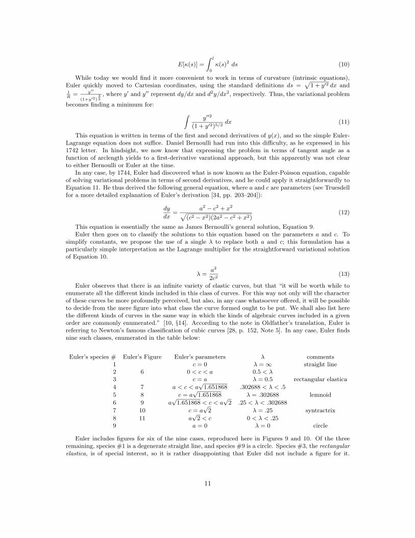
Euler observes that there is an infinite variety of elastic curves, but that “it will be worth while toenumerate all the different kinds included in this class of curves. For this way not only will the characterof these curves be more profoundly perceived, but also, in any case whatsoever offered, it will be possibleto decide from the mere figure into what class the curve formed ought to be put. We shall also list herethe different kinds of curves in the same way in which the kinds of algebraic curves included in a givenorder are commonly enumerated.” [10, §14]. According to the note in Oldfather’s translation, Euler isreferring to Newton’s famous classification of cubic curves [28, p. 152, Note 5]. In any case, Euler findsnine such classes, enumerated in the table below:

Euler’s species # Euler’s Figure Euler’s parameters λ comments1 c = 0 λ = ∞ straight line2 6 0 < c < a 0.5 < λ3 c = a λ = 0.5 rectangular elastica

4 7 a < c < a√

1.651868 .302688 < λ < .5

5 8 c = a√

1.651868 λ = .302688 lemnoid

6 9 a√

1.651868 < c < a√

2 .25 < λ < .302688

7 10 c = a√

2 λ = .25 syntractrix

8 11 a√

2 < c 0 < λ < .259 a = 0 λ = 0 circle

Euler includes figures for six of the nine cases, reproduced here in Figures 9 and 10. Of the threeremaining, species #1 is a degenerate straight line, and species #9 is a circle. Species #3, the rectangularelastica, is of special interest, so it is rather disappointing that Euler did not include a figure for it.

11

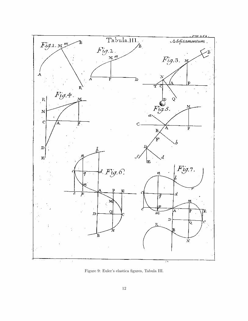
Figure 9: Euler’s elastica figures, Tabula III.

12

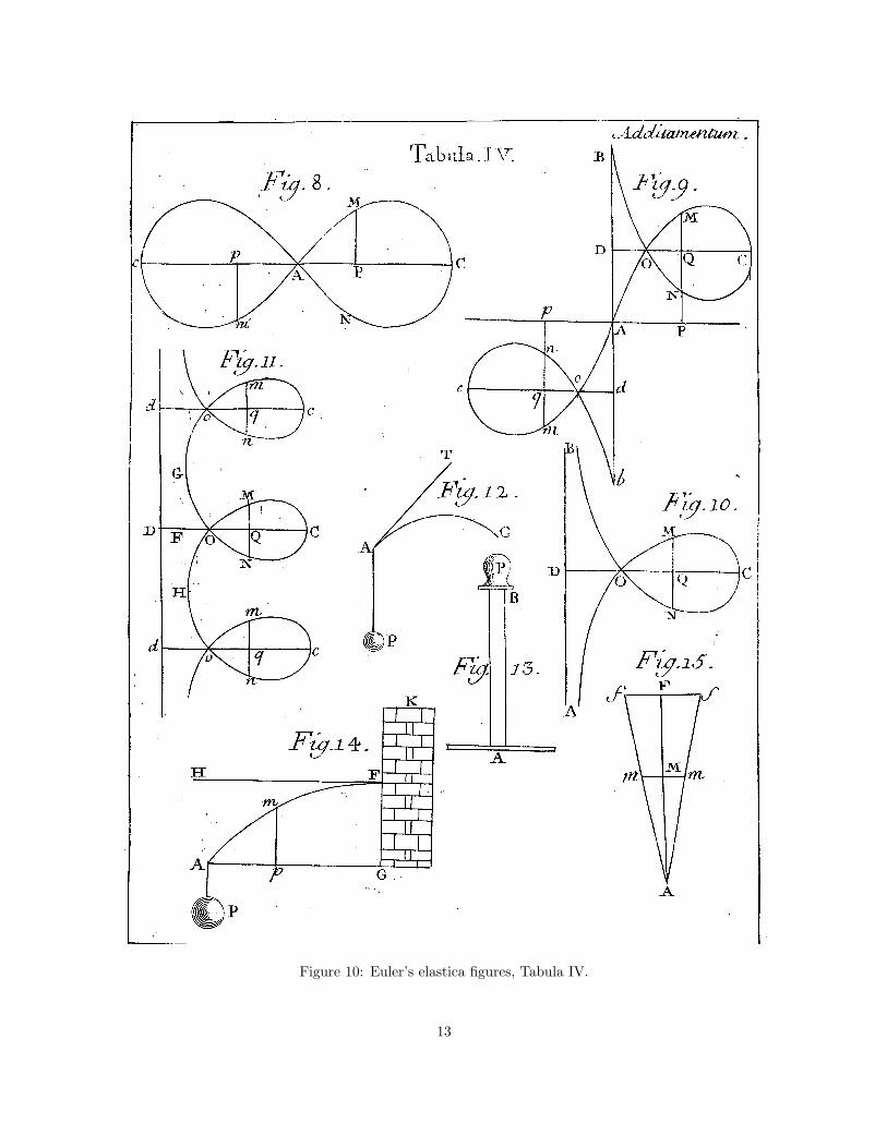
Figure 10: Euler’s elastica figures, Tabula IV.

13

Possibly, it was considered already known due to Bernoulli’s publication. Note also that in this specialcase, c = a, the equation becomes equivalent to Bernoulli’s Equation 2.

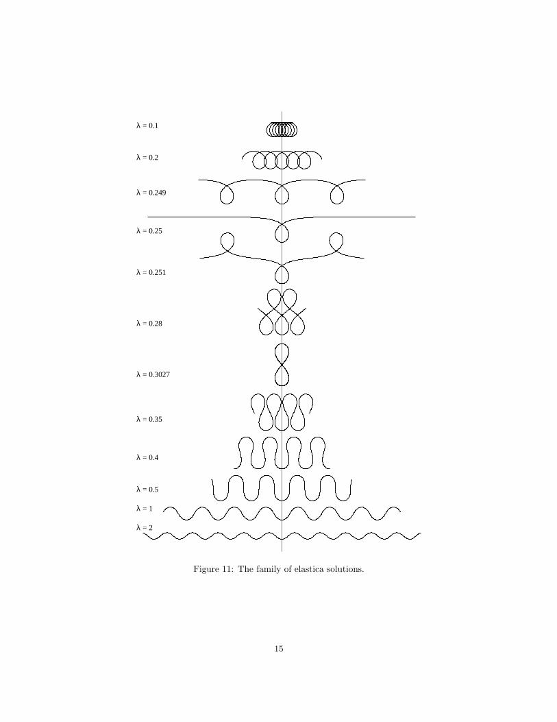
Compare these figures with the computer-drawn Figure 11. It is remarkable how clearly Euler wasable to visualize these curves, even 250 years ago. It is likely that the distortions and inaccuracies are dueprimarily to the draftsman engraving the figures for the book rather than to Euler himself; they displaylack of symmetry that Euler clearly would have known. In fact, Euler computed a number of values toseven or more decimal places, including the values of a and c for the lemnoid shape (species #5).

Note that for c2 < 2a2, or λ > .25, the inflectional cases, the equation is well-defined for −c < x < c.In these cases, the parameter c is half the width of the figure. In the non-inflectional cases (λ < .25), theequation has no solutions at x = 0, and in Euler’s figure the curve is drawn to the right of the y axis.

The curve described by species #7, the only nonperiodic solution, was known to Poleni in 1729, andis also known as the “syntractrix of Poleni,” or, in French, “la courbe des forcats” (the curve of convicts,or galley slaves). Euler gives its equation (in section 31) in closed form (without citing Poleni):

y =p

c2 − x2 − c

2log

c +√

c2 − x2

x(14)

9.1 Moments

Euler was also clearly aware of the simple moment approach to the elastica, and in section 43 of theAdditamentum, demonstrated its equivalence to the variational approach. To do so, he manipulated thequadrature formulation of the elastica, Equation 12, grouping all the terms involving first and second

derivatives of the curve into a single term Sq(1−p2)−32 . Recall that p = dy

dxand q = dp

dx= d2y

dx2 . Thus, thisterm is S times the curvature, yielding an equation relating curvature to Cartesian coordinates. Eulerexplains:

“But −(1+pp)3:2

qis the radius of curvature R; whence, by doubling the constants β and γ, the

following equation will arise:

S

R= α + βx− γy . (15)

This equation agrees admirably with that which the second or direct method supplies. Forlet α + βx − γy express the moment of the bending power, taking any line you please as anaxis, to which moment the absolute elasticity S, divided by the radius of curvature R mustbe absolutely equal. Thus, therefore, not only has the character of the elastic curve observedby the celebrated Bernoulli been most abundantly demonstrated, but also the very greatutility of my somewhat difficult formulas has been established in this example.”

This result certainly is confirmation of the variational technique, but in fairness it must be pointedout that James Bernoulli was able to derive essentially the identical equation (again, note the similaritybetween Equations 9 and 12) by using a combination of mechanical insight and clever integration.

10 Elliptic integrals

The elastica, having been present at the birth of the variational calculus, also played a major role in thedevelopment of another branch of mathematics: the theory of elliptic functions.

Even as the quadratures of these simple curves came to be revealed, analytic formulae for their lengthsremained elusive. The functions known by the first half of the 18th century were insufficient to determinethe length even of a curve as well-understood as an ellipse.

James Bernoulli set himself to this problem and was able to pose it succinctly (and even computeapproximate numerical values), if not fully solve it himself [32]. If the quadrature of a unit-excursionrectangular elastica is given by this equation:

y =

Z x

0

x2dx√1− x4

, (16)

then the arc length is given by:

14

λ = 0.1

λ = 0.2

λ = 0.249

λ = 0.25

λ = 0.251

λ = 0.28

λ = 0.3027

λ = 0.35

λ = 0.4

λ = 0.5

λ = 1

λ = 2

Figure 11: The family of elastica solutions.

15

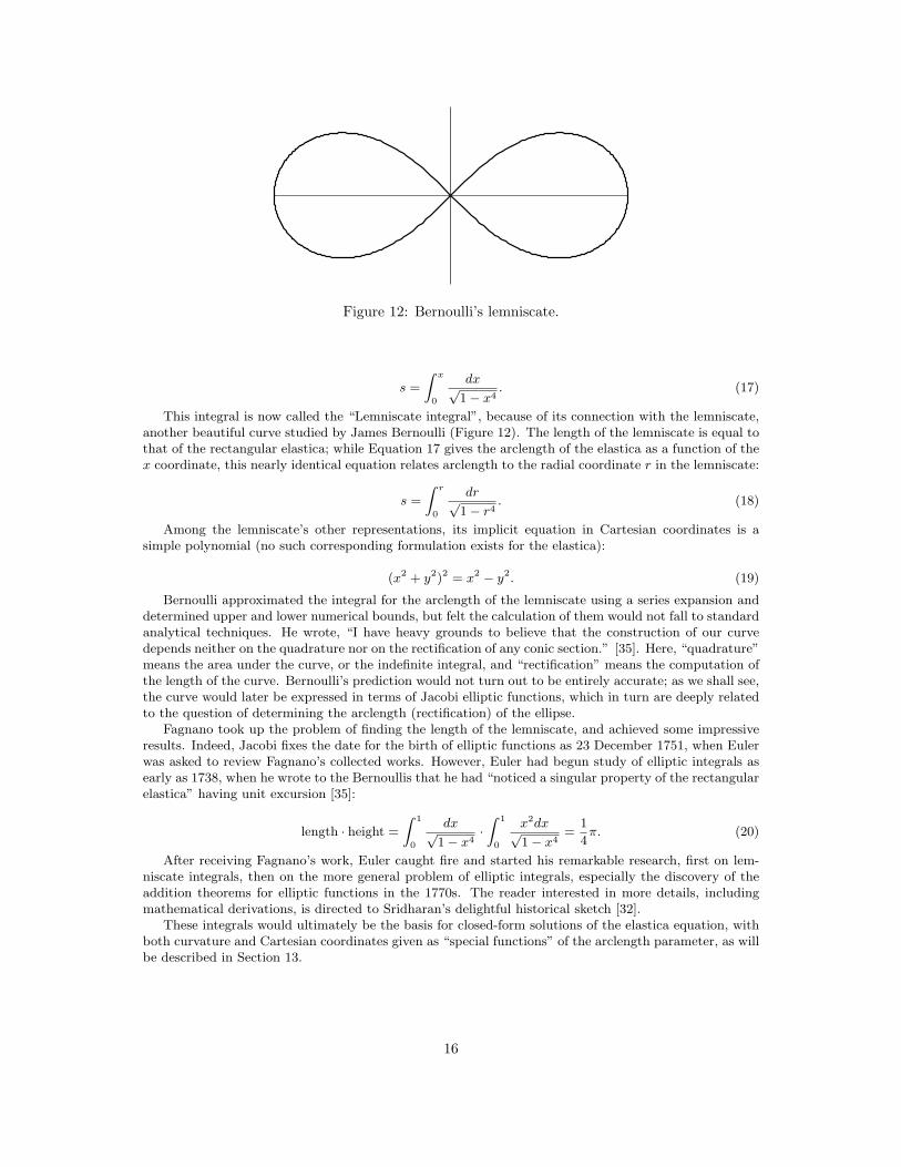
Figure 12: Bernoulli’s lemniscate.

s =

Z x

0

dx√1− x4

. (17)

This integral is now called the “Lemniscate integral”, because of its connection with the lemniscate,another beautiful curve studied by James Bernoulli (Figure 12). The length of the lemniscate is equal tothat of the rectangular elastica; while Equation 17 gives the arclength of the elastica as a function of thex coordinate, this nearly identical equation relates arclength to the radial coordinate r in the lemniscate:

s =

Z r

0

dr√1− r4

. (18)

Among the lemniscate’s other representations, its implicit equation in Cartesian coordinates is asimple polynomial (no such corresponding formulation exists for the elastica):

(x2 + y2)2 = x2 − y2. (19)

Bernoulli approximated the integral for the arclength of the lemniscate using a series expansion anddetermined upper and lower numerical bounds, but felt the calculation of them would not fall to standardanalytical techniques. He wrote, “I have heavy grounds to believe that the construction of our curvedepends neither on the quadrature nor on the rectification of any conic section.” [35]. Here, “quadrature”means the area under the curve, or the indefinite integral, and “rectification” means the computation ofthe length of the curve. Bernoulli’s prediction would not turn out to be entirely accurate; as we shall see,the curve would later be expressed in terms of Jacobi elliptic functions, which in turn are deeply relatedto the question of determining the arclength (rectification) of the ellipse.

Fagnano took up the problem of finding the length of the lemniscate, and achieved some impressiveresults. Indeed, Jacobi fixes the date for the birth of elliptic functions as 23 December 1751, when Eulerwas asked to review Fagnano’s collected works. However, Euler had begun study of elliptic integrals asearly as 1738, when he wrote to the Bernoullis that he had “noticed a singular property of the rectangularelastica” having unit excursion [35]:

length · height =

Z 1

0

dx√1− x4

·Z 1

0

x2dx√1− x4

=1

4π. (20)

After receiving Fagnano’s work, Euler caught fire and started his remarkable research, first on lem-niscate integrals, then on the more general problem of elliptic integrals, especially the discovery of theaddition theorems for elliptic functions in the 1770s. The reader interested in more details, includingmathematical derivations, is directed to Sridharan’s delightful historical sketch [32].

These integrals would ultimately be the basis for closed-form solutions of the elastica equation, withboth curvature and Cartesian coordinates given as “special functions” of the arclength parameter, as willbe described in Section 13.

16

11 Laplace on the capillary—1807

Remarkably, the elastica appears as yet another shape of the solution of a fundamental physics problem—the capillary. Pierre Simon Laplace investigated the equation for the shape of the capillary in his 1807Supplement au dixieme livre du Traite de mecanique celeste. Sur l’action capillaire7. See I. GrattanGuinness [15, p. 442] for a thorough description of these results. In particular, Laplace considers thesurface of a fluid trapped between two vertical plates, and obtains this equation (722.16 in [15]):

z′′ = 2(αz + b−1)(1 + z′2)3/2 (21)

Here, z represents height, and z′ and z′′ represent first and second derivatives with respect to thehorizontal coordinate. With suitable renaming of coordinates and substution of Equation 1 for curvaturein Cartesian coordinates, this equation can readily seen to be equivalent to Euler’s Equation 15.

Laplace also recognized that at least one instance of his equation was equivalent to the elastica. Hederives Equation 7 (save that Laplace writes Z for S) and notes that it is identical to the elastic curve[19, p. 379].

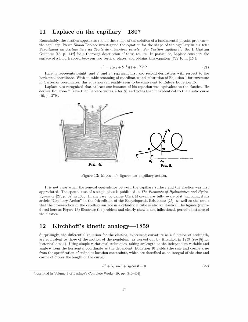
Figure 13: Maxwell’s figures for capillary action.

It is not clear when the general equivalence between the capillary surface and the elastica was firstappreciated. The special case of a single plate is published in The Elements of Hydrostatics and Hydro-dynamics [27, p. 32] in 1833. In any case, by James Clerk Maxwell was fully aware of it, including it hisarticle “Capillary Action” in the 9th edition of the Encyclopædia Britannica [25], as well as the resultthat the cross-section of the capillary surface in a cylindrical tube is also an elastica. His figures (repro-duced here as Figure 13) illustrate the problem and clearly show a non-inflectional, periodic instance ofthe elastica.

12 Kirchhoff’s kinetic analogy—1859

Surprisingly, the differential equation for the elastica, expressing curvature as a function of arclength,are equivalent to those of the motion of the pendulum, as worked out by Kirchhoff in 1859 (see [8] forhistorical detail). Using simple variational techniques, taking arclength as the independent variable andangle θ from the horizontal coordinate as the dependent, Equation 10 yields (the sine and cosine arisefrom the specification of endpoint location constraints, which are described as an integral of the sine andcosine of θ over the length of the curve):

θ′′ + λ1 sin θ + λ2 cos θ = 0 (22)

7reprinted in Volume 4 of Laplace’s Complete Works [19, pp. 349–401]

17

θ

r

F = mg

Fnet = mg sin θ

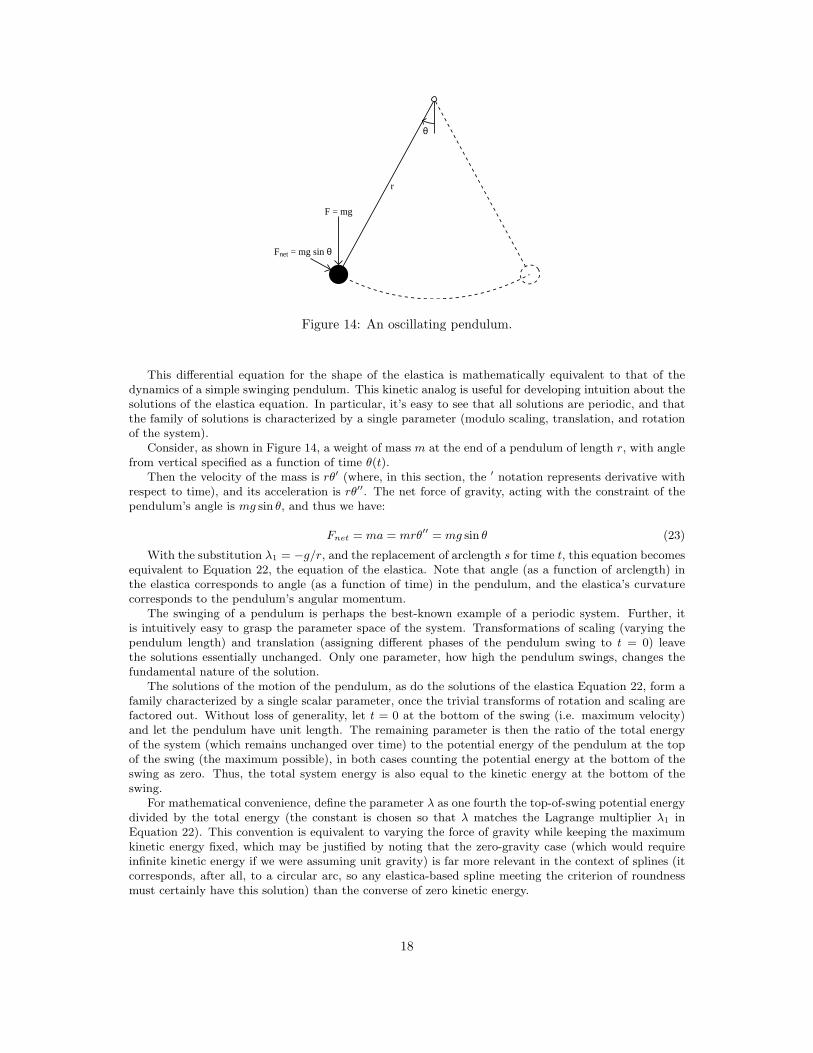
Figure 14: An oscillating pendulum.

This differential equation for the shape of the elastica is mathematically equivalent to that of thedynamics of a simple swinging pendulum. This kinetic analog is useful for developing intuition about thesolutions of the elastica equation. In particular, it’s easy to see that all solutions are periodic, and thatthe family of solutions is characterized by a single parameter (modulo scaling, translation, and rotationof the system).

Consider, as shown in Figure 14, a weight of mass m at the end of a pendulum of length r, with anglefrom vertical specified as a function of time θ(t).

Then the velocity of the mass is rθ′ (where, in this section, the ′ notation represents derivative withrespect to time), and its acceleration is rθ′′. The net force of gravity, acting with the constraint of thependulum’s angle is mg sin θ, and thus we have:

Fnet = ma = mrθ′′ = mg sin θ (23)

With the substitution λ1 = −g/r, and the replacement of arclength s for time t, this equation becomesequivalent to Equation 22, the equation of the elastica. Note that angle (as a function of arclength) inthe elastica corresponds to angle (as a function of time) in the pendulum, and the elastica’s curvaturecorresponds to the pendulum’s angular momentum.

The swinging of a pendulum is perhaps the best-known example of a periodic system. Further, itis intuitively easy to grasp the parameter space of the system. Transformations of scaling (varying thependulum length) and translation (assigning different phases of the pendulum swing to t = 0) leavethe solutions essentially unchanged. Only one parameter, how high the pendulum swings, changes thefundamental nature of the solution.

The solutions of the motion of the pendulum, as do the solutions of the elastica Equation 22, form afamily characterized by a single scalar parameter, once the trivial transforms of rotation and scaling arefactored out. Without loss of generality, let t = 0 at the bottom of the swing (i.e. maximum velocity)and let the pendulum have unit length. The remaining parameter is then the ratio of the total energyof the system (which remains unchanged over time) to the potential energy of the pendulum at the topof the swing (the maximum possible), in both cases counting the potential energy at the bottom of theswing as zero. Thus, the total system energy is also equal to the kinetic energy at the bottom of theswing.

For mathematical convenience, define the parameter λ as one fourth the top-of-swing potential energydivided by the total energy (the constant is chosen so that λ matches the Lagrange multiplier λ1 inEquation 22). This convention is equivalent to varying the force of gravity while keeping the maximumkinetic energy fixed, which may be justified by noting that the zero-gravity case (which would requireinfinite kinetic energy if we were assuming unit gravity) is far more relevant in the context of splines (itcorresponds, after all, to a circular arc, so any elastica-based spline meeting the criterion of roundnessmust certainly have this solution) than the converse of zero kinetic energy.

18

The potential energy at the top of the pendulum is 2mgr. The kinetic energy at the bottom of theswing is 1

2mv2, where, as above, v = rθ′. Thus, according to the definition above,

λ =1

4

2mgr1

2m(rθ′)2=

g

r(θ′)2

In other words, assuming (without loss of generality) unit pendulum length and unit velocity thebottom of the swing, λ simply represents the force of gravity. And this λ is the same as defined inEquation 13.

13 Closed form solution: Jacobi elliptic functions—1880

The closed-form solutions of the elastica, worked out by Saalschutz in 1880 [30], rely heavily on Jacobielliptic functions (see also [8] for more historical development, and Greenhill [16] for a contemporarypresentation of these results in English, suggesting the kinetic analog was a major motivator to derivingthe closed form solutions).

The Jacobi amplitude am(u, k) is defined as the inverse of the Jacobi elliptic integral of the first kind:

am(u, m) = the value of φ such that

u =

Z φ

0

1p1−m sin2 t

dt(24)

Here, m is known as the parameter. Jacobi elliptic functions are also commonly written in terms ofthe elliptic modulus k =

√m.

From this amplitude, the doubly periodic generalizations of the trigonometric functions follow:

sn(u, m) = sin(am(u, m)) (25)

cn(u, m) = cos(am(u, m)) (26)

dn(u, m) =q

1−m sin2(am(u, m)) (27)

Note that, when m is zero, sn and cn are equivalent to sin and cos, respectively, and when m is unity,sn and cn are equivalent to tanh and sech (1/cosh)([1, p. 571], §16.6).

13.1 Inflectional solutions

The closed form solutions are given separately for inflectional and non-inflectional cases. The intrinsicform, curvature as a function of arclength, is fairly simple:

dθ

ds= κ = 2

√m cn(s, m), (28)

Expressing the curve in the form of angle as a function of arclength is also straightforward:

sin1

2θ =

√m sn(s, m) (29)

Through an impressive feat of analysis, the curve can be expressed in cartesian coordinates as afunction of arclength. First, we’ll need the elliptic integral of the second kind, E(φ, k):

E(φ, k) =

Z φ

0

p1−m sin2 θ dθ (30)

x(s) = s− 2E(am(s, m), m)y(s) = −2

√m cn(s, m)

(31)

In Love’s presentation of these results, E(am(s, m), m) is defined in terms of an integral of dn(u, m).The equivalence with Equation 30 follows through a standard identity of the Jacobi elliptical functions([1, p. 576], 16.26.3).

19

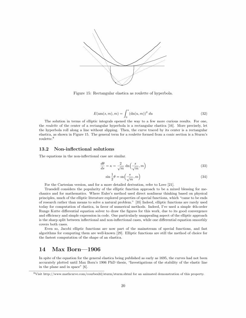
Figure 15: Rectangular elastica as roulette of hyperbola.

E(am(s, m), m) =

Z s

0

(dn(u, m))2 du (32)

The solution in terms of elliptic integrals opened the way to a few more curious results. For one,the roulette of the center of a rectangular hyperbola is a rectangular elastica [16]. More precisely, letthe hyperbola roll along a line without slipping. Then, the curve traced by its center is a rectangularelastica, as shown in Figure 15. The general term for a roulette formed from a conic section is a Sturm’sroulette.8

13.2 Non-inflectional solutions

The equations in the non-inflectional case are similar.

dθ

ds= κ =

2√m

dn“ s√

m, m

”(33)

sin1

2θ = sn

“ s√m

, m”

(34)

For the Cartesian version, and for a more detailed derivation, refer to Love [21].Truesdell considers the popularity of the elliptic function approach to be a mixed blessing for me-

chanics and for mathematics. Where Euler’s method used direct nonlinear thinking based on physicalprinciples, much of the elliptic literature explored properties of special functions, which “came to be endsof research rather than means to solve a natural problem.” [35] Indeed, elliptic functions are rarely usedtoday for computation of elastica, in favor of numerical methods. Indeed, I’ve used a simple 4th-orderRunge Kutte differential equation solver to draw the figures for this work, due to its good convergenceand efficiency and simple expression in code. One particularly unappealing aspect of the elliptic approachis the sharp split between inflectional and non-inflectional cases, while one differential equation smoothlycovers both cases.

Even so, Jacobi elliptic functions are now part of the mainstream of special functions, and fastalgorithms for computing them are well-known [29]. Elliptic functions are still the method of choice forthe fastest computation of the shape of an elastica.

14 Max Born—1906

In spite of the equation for the general elastica being published as early as 1695, the curves had not beenaccurately plotted until Max Born’s 1906 PhD thesis, “Investigations of the stability of the elastic linein the plane and in space” [6].

8Visit http://www.mathcurve.com/courbes2d/sturm/sturm.shtml for an animated demonstration of this property.

20

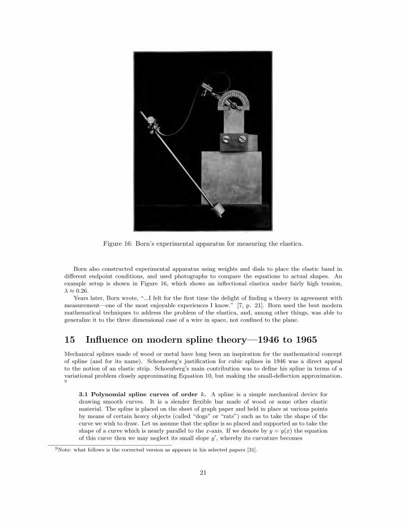
Figure 16: Born’s experimental apparatus for measuring the elastica.

Born also constructed experimental apparatus using weights and dials to place the elastic band indifferent endpoint conditions, and used photographs to compare the equations to actual shapes. Anexample setup is shown in Figure 16, which shows an inflectional elastica under fairly high tension,λ ≈ 0.26.

Years later, Born wrote, “...I felt for the first time the delight of finding a theory in agreement withmeasurement—one of the most enjoyable experiences I know.” [7, p. 21]. Born used the best modernmathematical techniques to address the problem of the elastica, and, among other things, was able togeneralize it to the three dimensional case of a wire in space, not confined to the plane.

15 Influence on modern spline theory—1946 to 1965

Mechanical splines made of wood or metal have long been an inspiration for the mathematical conceptof spline (and for its name). Schoenberg’s justification for cubic splines in 1946 was a direct appealto the notion of an elastic strip. Schoenberg’s main contribution was to define his spline in terms of avariational problem closely approximating Equation 10, but making the small-deflection approximation.9

3.1 Polynomial spline curves of order k. A spline is a simple mechanical device fordrawing smooth curves. It is a slender flexible bar made of wood or some other elasticmaterial. The spline is placed on the sheet of graph paper and held in place at various pointsby means of certain heavy objects (called “dogs” or “rats”) such as to take the shape of thecurve we wish to draw. Let us assume that the spline is so placed and supported as to take theshape of a curve which is nearly parallel to the x-axis. If we denote by y = y(x) the equationof this curve then we may neglect its small slope y′, whereby its curvature becomes

9Note: what follows is the corrected version as appears in his selected papers [31].

21

1/R = y′′/(1 + y′2)3/2 ≈ y′′

The elementary theory of the beam will then show that the curve y = y(x) is a polygonal linecomposed of cubic arcs which join continuously, with a continuous first and second derivative10.These junction points are precisely the points where the heavy supporting objects are placed.

While Schoenberg’s splines are excellent for fitting the values of functions (the problem of appoxima-tion), it was clear that they were not ideal for representing shapes. Birkhoff and de Boor wrote in 1965[5] that “linearized interpolation schemes have a basic shortcoming: they are not intrinsic geometricallybecause they are not invariant under rigid rotation. Physically it seems more natural to replace linearizedspline curves by non-linear splines (or “elastica”), well known among elasticians,” citing Love [21] as anauthority. They also stated the result that in a mechanical spline constrained to pass through the controlpoints only by pure normal forces, only the rectangular elastica is needed.

Birkhoff and de Boor also noted some shortcomings in the elastica as a replacement for the mechanicalspline, particularly the lack of an existence and uniqueness theory for non-linear spline curves with givenendpoints, endslopes, and sequence of internal points. Indeed, they state that “nor does it seem particu-larly desirable” to have techniques for intrinsic splines approximate the elastica, and they proposed othertechniques, such as Hermite interpolation by segments of Euler spirals joined together with continuouscurvature.

According to notes taken by Stanford professor George Forsythe [11], in the conference presentationof this work, they also referenced Max Born’s PhD thesis [6], and also described a goal of the work asproviding an “automatic French curve.” The presentation must have made an impression on Forsythe,judging from the laconic sentence, “Deep.” Forsythe, working with his colleague Erastus Lee from theMechanical Engineering college at Stanford, would go on to analyze the nonlinear spline considerablymore deeply, deriving it from both the variational formulation of Equation 10 and an exploration ofmoments, normal forces, and longitudinal forces [20]. That publication also included a result for energyminimization in the case where the elastica is a closed loop.

16 Numerical techniques—1958 through today

The arrival of the high-speed digital computer created a strong demand for efficient algorithms to computethe elastica, particularly to compute the shape of an idealized spline constrained to pass through asequence of control points.

Birkhoff and de Boor [5] cited several approximations to non-linear splines, including those of Fowlerand Wilson [12] and MacLaren [22] at Boeing in 1959, and described their own work along similar lines.None of these was a particularly precise or efficient approximation.

Around the same time, and very possibly working independently, Mehlum and others designed theAutokon system [26] using an approximation to the elastica (called the kurgla 1 algorithm). However,this algorithm was not an accurate simulation of the mechanical spline, as did not minimize the totalbending energy of the curve, and, in fact, could generate (approximations to) the entire family of elasticacurves in service of its splines. An objection to this technique is that the spline was not extensional;adding a new control point conciding with the generated spline would slightly perturb the curve. Thus,this approximate elastica was soon replaced by the kurgla 2 algorithm implementing precisely the Eulerspiral Hermite interpolation suggested by Birkhoff and de Boor.

A sequence of papers refining the numerical techniques for computing the elastica-based nonlinearspline followed: Glass in 1966 [14], Woodford in 1969 [38], Malcolm in 1977 [23]. Most of these involvediscretized formulations of the problem. Interestingly, Malcolm reports that Larkin developed a techniquebased on direct evaluation of the Jacobi elliptic integrals which is nonetheless “probably quite slow”compared with the discretized approaches, “due to the large number of transcedental functions whichmust be evaluated.” Malcolm’s paper contains a good survey of known numerical techniques, and isrecommended to the reader interested in following this development in more detail.

In spite of the fairly rich literature available on the elastica, at least one researcher, B. K. P. Horn in1981, seems to have independently derived the rectangular elastica from the principle of minimizing the

10Schoenberg is indebted for this suggestion to Professor L. H. Thomas of Ohio State University.

22

strain energy [18], going through an impressive series of derivations, and using the full power of ellipticintegral theory, to arrive at exactly the same integral as Bernoulli had derived almost three hundredyears previously.

Edwards [9] proposes a spline solution in which the elastica in the individual segments are computedusing Jacobi elliptic functions. He also gives a global solver based on a Newton technique, each iterationof which solves a band-diagonal Jacobian matrix. A particular concern was exploring the cases when nostable solution exists, a weakness of the elastica-based spline compared to other techniques. Edwardsclaims that his numerical techniques would always converge on a solution if one exists.

17 Sources and acknowledgements

This historical sketch draws heavily on Truesdell’s history in an introduction to Ser 2, Volume X ofEuler’s Opera Omnia [34]. Indeed, a careful reading of that work reveals virtually all that needs to beknown about the problem of the elastica and its historical development through the time of Euler.

Euler’s 1744 Additamentum is a truly remarkable work, deserving of deep study. The original Latinis available in facsimile thanks to the Euler archive, but the 1933 English translation by Oldfather [28]makes it much more understandable to the English-speaking reader.

I am deeply grateful to Alex Stepanov, Seth Schoen, Martin Meijering and Ben Fortson for help withthe translations from the Latin. Special mention is also due the excellent “Latin words” program byWilliam Whitaker, which lets anyone with a rudimentary knowledge of Latin and a good deal of patienceand determination puzzle out the meaning of a text. Of course, all errors in translation are my ownresponsibility.

Patricia Radelet has been most helpful in supplying high-quality images for James Bernoulli’s originalfigures, reproduced here as Figures 4 and 5, and for providing scans of the original text of his 1694publication.

Thanks also to the Stanford Special Collections Library for giving me access to Prof. Forsythe’s notesand correspondence, which were invaluable in tracing the influence of the elastica through early work onnon-linear splines.

References

[1] Milton Abramowitz and Irene A. Stegun. Handbook of Mathematical Functions with Formulas,Graphs, and Mathematical Tables. Dover, New York, ninth Dover printing, tenth GPO printingedition, 1964.

[2] Daniel Bernoulli. The 26th letter to Euler. In Correspondence Mathematique et Physique, volume 2.P. H. Fuss, October 1742.

[3] James Bernoulli. Quadratura curvae, e cujus evolutione describitur inflexae laminae curvatura. InDie Werke von Jakob Bernoulli, pages 223–227. Birkhauser, 1692. Med. CLXX; Ref. UB: L Ia 3, p211–212.

[4] James Bernoulli. Jacobi Bernoulli, Basilieensis, Opera, volume 1. Cramer & Philibert, Geneva,1744.

[5] Garrett Birkhoff and Carl R. de Boor. Piecewise polynomial interpolation and approximation. Proc.General Motors Symp. of 1964, pages 164–190, 1965.

[6] Max Born. Untersuchungen uber die Stabilitat der elastischen Linie in Ebene und Raum, underverschiedenen Grenzbedingungen. PhD thesis, University of Gottingen, 1906.

[7] Max Born. My Life and Views. Scribner, 1968.

[8] Lawrence D’Antonio. The fabric of the universe is most perfect: Euler’s research on elastic curves.In Euler at 300: an appreciation, pages 239–260. Mathematical Association of America, 2007.

[9] John A. Edwards. Exact equations of the nonlinear spline. Trans. Mathematical Software, 18(2):174–192, June 1992.

23

[10] Leonhard Euler. Methodus inveniendi lineas curvas maximi minimive proprietate gaudentes, sivesolutio problematis isoperimetrici lattissimo sensu accepti, chapter Additamentum 1. eulerarchive.orgE065, 1744.

[11] G. Forsythe. Notes taken at the GM Research Laboratories Symposium on approximation of func-tions, special collection SC98 2-6, 1964.

[12] A. H. Fowler and C. W. Wilson. Cubic spline, a curve fitting routine. Technical Report Y-1400,Oak Ridge Natl. Laboratory, September 1962.

[13] Craig G. Fraser. Mathematical technique and physical conception in Euler’s investigation of theelastica. Centaurus, 34(3):211–246, 1991.

[14] J. M. Glass. Smooth curve interpolation: A generalized spline-fit procedure. BIT, 6(4):277–293,1966.

[15] I. Grattan-Guinness. Convolutions in French Mathematics, 1800–1840. Birkhauser, 1990.

[16] Alfred George Greenhill. The Applications of Elliptic Functions. Macmillan, London, 1892.

[17] Peter M. Harman and Alan E. Shapiro, editors. The critical role of curvature in Newton’s developingdynamics. Cambridge University Press, 2002.

[18] B. K. P. Horn. The curve of least energy. Technical Report A.I. Memo. No. 612, MIT AI Lab,January 1981.

[19] Pierre Simon Laplace. Œuvres completes de Laplace, volume 4. Gauthier-Villars, 1880.

[20] Erastus H. Lee and George E. Forsythe. Variational study of nonlinear spline curves. SIAM Rev.,15(1):120–133, 1973.

[21] A. E. H. Love. A Treatise on the Mathematical Theory of Elasticity. Dover Publications, fourthedition, 1944.

[22] D. H. MacLaren. Formulas for fitting a spline curve through a set of points. Technical Report 2,Boeing Appl. Math. Report, 1958.

[23] Michael A. Malcolm. On the computation of nonlinear spline functions. SIAM J. Numer. Anal.,14(2):254–282, April 1977.

[24] Dan Margalit. History of curvature. http://www3.villanova.edu/maple/misc/history of curvature/k.htm,2003.

[25] James Clerk Maxwell. Capillary action. In Encyclopædia Britannica, pages 256–275. Henry G.Allen, 9th edition, 1890.

[26] Even Mehlum. Nonlinear splines. Computer Aided Geometric Design, pages 173–205, 1974.

[27] William Hallowes Miller. The Elements of Hydrostatics and Hydrodynamics. J. & J. J. Deighton,1831.

[28] W. A. Oldfather, C. A. Ellis, and Donald M. Brown. Leonhard Euler’s elastic curves. Isis, 20(1):72–160, November 1933.

[29] William H. Press, Saul A. Teukolsky, William T. Vetterling, and Brian P. Flannery. NumericalRecipes in C. Cambridge University Press, 2nd edition, 1992.

[30] Louis Saalschutz. Der belastete Stab unter Einwirkung einer seitlichen Kraft. B. G. Teubner, Leipzig,1880.

[31] I. J. Schoenberg. Selected Papers, volume I. Birkhauser, Boston, 1988. edited by Carl de Boor.

[32] R Sridharan. Physics to mathematics: from lintearia to lemniscate – I. Resonance, pages 21–29,April 2004.

[33] Isaac Todhunter. A History of the Theory of Elasticity and of the Strength of Materials, volume 1.Cambridge University Press, 1886.

[34] C. Truesdell. The Rational Mechanics of Flexible or Elastic Bodies: 1638–1788. Leonhard Euler,Opera Omnia. Birkhauser, 1960.

[35] C. Truesdell. The influence of elasticity on analysis: The classic heritage. Bull. AMS, 9(3):293–310,November 1983.

24

[36] C. Truesdell. Der Briefwechsel von Jacob Bernoulli, chapter Mechanics, especially Elasticity, in theCorrespondence of Jacob Bernoulli with Leibniz. Birkhauser, 1987.

[37] William Whewell. Analytical Statics: A supplement to the fourth edition of an elementary treatiseon Mechanics. J. & J. J. Deighton, Cambridge, England, 1833.

[38] C. H. Woodford. Smooth curve interpolation. BIT, 9:69–77, 1969.

25