a mass conservative and water storage consistent variable
TRANSCRIPT

Hydrol Earth Syst Sci 11 1645ndash1659 2007wwwhydrol-earth-syst-scinet1116452007copy Author(s) 2007 This work is licensedunder a Creative Commons License
Hydrology andEarth System
Sciences
A mass conservative and water storage consistent variableparameter Muskingum-Cunge approach
E Todini
Department of Earth and Geo-Environmental Sciences University of Bologna Italy
Received 23 May 2007 ndash Published in Hydrol Earth Syst Sci Discuss 12 June 2007Revised 11 September 2007 ndash Accepted 1 October 2007 ndash Published 15 October 2007
Abstract The variable parameter Muskingum-Cunge (MC)flood routing approach together with several variants pro-posed in the literature does not fully preserve the massbalance particularly when dealing with very mild slopes(lt10minus3) This paper revisits the derivation of the MC anddemonstrates (i) that the loss of mass balance in MC iscaused by the use of time variant parameters which violatethe implicit assumption embedded in the original derivationof the Muskingum scheme which implies constant parame-ters and at the same time (ii) that the parameters estimated bymeans of the Cunge approach violate the two basic equationsof the Muskingum formulation The paper also derives themodifications needed to allow the MC to fully preserve themass balance and at the same time to comply with the orig-inal Muskingum formulation in terms of water storage Theproperties of the proposed algorithm have been assessed byvarying the cross section the slope the roughness the spaceand the time integration steps The results of all the tests alsoshow that the new algorithm is always mass conservativeFinally it is also shown that the proposed approach closelyapproaches the full de Saint Venant equation solution bothin terms of water levels and discharge when the parabolicapproximation holds
1 Introduction
In 1938 McCarthy (1938 1940) proposed an original ldquohy-drologicalrdquo flood routing method which has become quitepopular under the name of the Muskingum approach Theattribute ldquohydrologicalrdquo to a flood routing model generallyindicates that a finite river reach is taken into account by solv-ing directly for the outflow discharges as a function of theinflow ones while all the geomorphological characteristics
Correspondence toE Todini(eziotodiniuniboit)
and the hydraulic properties of the reach are lumped into anumber of model parameters For instance other ldquohydrolog-icalrdquo modelling approaches to flood routing are the DiffusionAnalogy response function model (Hayami 1951 Dooge1973 Todini and Bossi 1986) the cascade of linear reser-voirs (Nash 1958) whose applicability to flood routing wasdemonstrated by Kalinin and Miljukov (1958) or the cascadeof non-linear reservoirs developed as part of the TOPKAPIhydrological model (Liu and Todini 2002 2004)
In 1969 Cunge extended the Muskingum method to timevariable parameters whose values could be determined as afunction of a reference discharge by recognizing that theoriginal Muskingum approach could be viewed as a first or-der kinematic approximation of a diffusion wave model butthen converting it into a parabolic approach by proposing aparticular estimation of its parameter values which wouldguarantee that the real diffusion would be equalled by thenumerical diffusion
The method has been widely and successfully used for dis-charge routing notwithstanding the fact that several authorspointed out that the approach displays a mass balance errorthat can reach values of 8 to 10 (Tang et al 1999 Tang andSamuels 1999) Although many authors worked on the prob-lem of the mass balance inconsistency (Ponce and Yevjevich1978 Koussis 1983 Ponce and Chaganti 1994 Tang et al1999 Tang and Samuels 1999 Perumal et al 2001) a con-clusive and convincing reason was not demonstrated
In addition to the lack of mass balance an even more im-portant inconsistency is generated by the variable parame-ter Muskingum known as the Muskingum-Cunge (MC) ap-proach which apparently has never been reported in the liter-ature if one substitutes back into the Muskingum equationsthe parameters derived using Cunge approach two differentand inconsistent values for the water volume stored in thechannel are obtained
The above mentioned pitfalls of MC approach have pro-vided the motivation for this paper and it was deemed
Published by Copernicus Publications on behalf of the European Geosciences Union
1646 E Todini Mass conservartive Muskingum-Cunge
essential to revisit the Muskingum-Cunge model in order tofind the causes and possibly to overcome the inconsistenciessince after 37 years from its development the MC methodhas still a fundamental role in modern hydrology First ofall the MC is widely used as the routing component of sev-eral distributed or semi-distributed hydrological models inwhich case the preservation of the mass balance is an essen-tial feature Moreover although several (more or less ex-pensive) computer packages are available today that solvethe full de Saint Venant equations (for instance SOBEK ndashStelling and Duinmeijer 2003 Stelling and Verwey 2005MIKE11 ndash DHI Water amp Environment 2000 HEC-RAS ndashUS Army Corps of Engineers 2005 and many others) thevariable parameter MC is still widely used all throughoutthe world when the lack of knowledge of river cross sectionsdoes not justify the use of more complex routing models An-other attractive reason is that it can be easily programmed atpractically no cost
This paper describes the analysis that was carried out andthe corrections that were found to be appropriate The qual-ity of the new results was then assessed by routing a testwave specifically the asymmetrical wave proposed by Tanget al (1999) through three channels with different cross sec-tions (rectangular triangular and trapezoidal) by varying theslope the roughness the space and time integration inter-vals All the results obtained show that the new approachin all the cases fully complies with the requirements of pre-serving mass balance and at the same time of satisfying theMuskingum equations
Finally a comparison with MIKE11 (DHI Water amp Envi-ronment 2000) shows that when the parabolic approxima-tion holds the proposed algorithm is capable of closely ap-proximating the full de Saint Venant equations results bothin terms of discharge and water levels This is obviously trueprovided that the original limitations of the kinematic wavemodel and of the Muskingum model in all its variants aretaken into account namely the approach can only be appliedin river or channel reaches not affected by the downstreamconditions and backwater effects
2 The derivation of the Muskingum variable parameterequations
The derivation of the original Muskingum approach is basedupon the following two equations (Eq 1) written for achannel (or river) reach without lateral inflow
dSdt
= I minus O
S = k ε I + k (1 minus ε) O
(1a)(1b)
The first equation (Eq 1a) represents the mass balanceglobally applied to the reach between the upstream andthe downstream sections while the second one (Eq 1b)expressesS [L3
] the volume stored in the reach as a simple
linear combination ofI [L3T minus1] the inflow discharge at the
upstream section andO [L3T minus1] the outflow discharge at
the downstream section In Eq (1)k [T ] andε [dimension-less] are the two model parameters to be determined fromthe observations It will be noticed that the two Muskingumequations define the storageS and its derivativedS
dtas a
function of the inflowI and outflowO discharges as well asof the two parametersk andε
Note that although the original derivation assumes thatthe very basis of the Muskingum routing procedure is thatthe storage consists of both ldquoprismrdquo (level pool) storageand ldquowedgerdquo storage that reflects the imbalance between in-flow and outflow (eg Chow 1964 Chow et al 1988) themodel can be more proficiently thought of as a two param-eter ldquolumpedrdquo model at the river reach scale the storage ofwhich can be expressed at any point in time as in Eq (1b)
In the classical derivation of the Muskingum model thesecond expression in Eq (1b) is substituted into the first oneto give
d [k ε I ]
dt+
d [k (1 minus ε) O]
dt= I minus O (2)
and by assuming thatk andε are constant in time one canwrite
k εdI
dt+k (1 minus ε)
dO
dt= I minus O (3)
Equation (3) is then solved using a centred finite differenceapproach by expressing the various quantities as follows
I =It+1t + It
2 O =
Ot+1t + Ot
2
dI
dt=
It+1t minus It
1t
dO
dt=
Ot+1t minus Ot
1t(4)
Substitution in Eq (3) of the quantities defined in Eq (4)yields
k εIt+1t minus It
1t+ k (1 minus ε)
Ot+1t minus Ot
1t
=It+1t + It
2minus
Ot+1t + Ot
2(5)
By multiplying both sides by 21t the following expressioncan be found
2 k ε (It+1tminusI t ) +2 k (1minusε) (Ot+1tminusO t )
= 1t (It+1t+I t ) minus1t (Ot+1t+O t ) (6)
which can be rewritten as
[2 k (1minusε) +1t ] O t+1t= [minus2 k ε+1t ] I t+1t
+ [2 k ε+1t ] It+ [2 k (1minusε) minus1t ] Ot (7)
to give
Ot+1t =minus2 k ε + 1t
2 k (1 minus ε) + 1tIt+1t +
2 k ε + 1t
2 k (1 minus ε) + 1tIt
+2 k (1 minus ε) minus 1t
2 k (1 minus ε) + 1tOt (8)
Hydrol Earth Syst Sci 11 1645ndash1659 2007 wwwhydrol-earth-syst-scinet1116452007
E Todini Mass conservartive Muskingum-Cunge 1647
Finally Eq (8) can be rewritten as
Ot+1t= C1It+1t+C2It+C3Ot (9)
with the following substitutions
C1 =minus2 k ε + 1t
2 k (1 minus ε) + 1t C2 =
2 k ε + 1t
2 k (1 minus ε) + 1t
C3 =2 k (1 minus ε) minus 1t
2 k (1 minus ε) + 1t(10)
whereC1 C2 andC3 are three coefficients subject to the fol-lowing property
C1 + C2 + C3 = 1 (11)
as can be easily verifiedCunge (1969) extended the original Muskingum method to
time variable parameters whose values could be determinedas a function of a reference discharge The clever idea ofCunge was to recognize that Eq (9) of the original Musk-ingum approach was formally the same and could be inter-preted either as a kinematic wave model (a first order approx-imation of a diffusion wave model) or as a proper diffusivewave model depending on the value of the adopted parame-ters He also showed how Eq (9) could be transformed into aproper diffusion wave model by introducing the appropriatediffusive effect through a particular estimation of the modelparameter values Cunge started from the following kine-matic routing model
partQ
partt+ c
partQ
partx= 0 (12)
whereQ[L3T minus1
]is the dischargex [L] the longitudinal
coordinatet [T ] the time coordinate andc[LT minus1
]the
celerity He derived the following classical finite differenceweighted approximation for the partial derivatives on a fourpoints scheme
partQ
parttasymp
ε(Qi+1
j minus Qij
)+ (1 minus ε)
(Qi+1
j+1 minus Qij+1
)1t
(13)
partQ
partxasymp
ϑ(Qi+1
j+1 minus Qi+1j
)+ (1 minus ϑ)
(Qi
j+1 minus Qij
)1x
(14)
whereQi+1j+1=Q ((i + 1) 1t (j+1) 1x) Qi+1
j
=Q ((i+1) 1t j1x) Qij+1=Q (i1t (j+1) 1x)
Qij=Q (i1t j1x) ε (0leεle1) being the space weight-
ing factor andϑ (0leϑle1) the time weighting factorThis approximation leads to the following first order ap-
proximation of the kinematic wave equation (Eq 12)
ε(Qi+1
j minus Qij
)+ (1 minus ε)
(Qi+1
j+1 minus Qij+1
)1t
+cϑ
(Qi+1
j+1 minus Qi+1j
)+ (1 minus ϑ)
(Qi
j+1 minus Qij
)1x
= 0 (15)
which can be rewritten as
ε(Qi+1
j minus Qij
)+ (1 minus ε)
(Qi+1
j+1 minus Qij+1
)1t
+c
2
(Qi+1
j+1 minus Qi+1j
)+
(Qi
j+1 minus Qij
)1x
= 0 (16)
by assuming a time centered scheme(ϑ=
12
)
Equation (16) after some algebraic manipulation can betransformed into
Qi+1j+1 = C1Q
i+1j + C2Q
ij + C3Q
ij+1 (17)
where
C1 =minus21xε + c1t
21x (1 minus ε) + c1t C2 =
21xε + c1t
21x (1 minus ε) + c1t
C3 =21x (1 minus ε) minus c1t
21x (1 minus ε) + c1t(18)
Cunge also noted that substituting fork=1xc
and by taking
Ot+1t=Qi+1j+1 Ot=Qi
j+1 It+1t=Qi+1j It=Qi
j Eq (17)becomes identical to Eq (9) Nevertheless one should beaware that these two equations have a totally different mean-ing While Eq (17) represents the solution of a partial dif-ferential equation Eq (9) is the solution of an ordinary dif-ferential equation after integration of the continuity of massequation in space
As a matter of fact a formally similar equation althoughwith different parameter values can also be obtained fromthe discretisation of any explicit parabolic or hyperbolicscheme This is what gave to Cunge (1969) the idea for de-riving his variable parameter formulation by expanding thedischargeQ in Taylor series he showed that Eq (17) repre-sents a first order approximation with second order residualequal zero of the kinematic model given in Eq (12) and atthe same time a linear approximation of the parabolic modelof Eq (19)
partQ
partt+ c
partQ
partxminus
Q
2BS0
part2Q
partx2= 0 (19)
with second order rounding error (also known as numericaldiffusion) given by
R =c1x
2(1 minus 2ε)
part2Q
partx2+ middot middot middot middot middot (20)
In Eq (19)B [L] is the surface widthS0 [dimensionless]the bottom slope
This result implies that Eq (17) can also be interpreted asthe solution of the parabolic model given in Eq (19) pro-vided that the following relation holds
c1x
2(1 minus 2ε) =
Q
2BS0(21)
wwwhydrol-earth-syst-scinet1116452007 Hydrol Earth Syst Sci 11 1645ndash1659 2007
1648 E Todini Mass conservartive Muskingum-Cunge
0 12 24 36 48 60 72 84 960
05
1
15
2
25
3x 10
6
Time [hours]
Wat
er S
tora
ge [m
3 ]
Water Storage
Steady State
MC - Eqn 26
MC - Eqn 27
Fig 1 Steady state volume (solid line) and storage volumes com-puted using Eq (26) (dashed line) and Eq (27) (dotted line)
Therefore by imposing that the numerical diffusion equalsthe physical one (see also Szel and Gaspar 2000 Wang etal 2006) Cunge (1969) derived an expression forε
ε =1
2
(1 minus
Q
c1xBS0
)(22)
which was used together withk=1xc
in Eq (18) and up-dated at each time step to give rise to the so called VariableParameter Muskingum-Cunge approach Successively with-out changing the nature of the problem Ponce and Yevjevichproposed (1978) the following expressions forC1 C2 C3
C1=minus1+C+D
1+C+D C2=
1+CminusD
1+C+D C3=
1minusC+D
1+C+D(23)
derived in terms of the dimensionless ldquoCourant numberrdquo(C)and ldquocell Reynolds numberrdquo(D) which is the ratio of thephysical and numerical diffusivities
C =c1t
1x D =
Q
B S0 c 1x(24)
Several ways for estimatingQ andc have been also proposedin the literature (Ponce and Chaganti 1994 Tang et al 1999Wang et al 2006) giving rise to a wide variety of three orfour point schemes
ParametersC andD are generally estimated at each timeinterval as a function of a reference dischargeQ relevant toeach computation section in which a river reach will be di-vided This poses certain limitations on the length1x of thecomputation sectionQ which will be evaluated at a cen-tral point will be used to estimate the water stage and theother quantities of interest such asB c and finallyC andD The larger1x is the likelihood that the Muskingum hy-pothesis on the linear variation in space of the discharge will
hold decreases Although this property is also influenced bybed slope friction and surface width as a rule of thumb oneshould never exceed few kilometers (possibly one) to avoiderrors which will be more evident in terms of water stage
By comparing Eq (10) and Eq (23) one can finally derivethe expressions for the two original Muskingum parameters
k =1tC
ε =1minusD
2
(25a)(25b)
The model with the two parameters estimated in everycomputation section of length1x and at each time step1t
according to Eqs (25) is known as the Muskingum-Cunge(MC) method and has been and still is widely used all overthe world for routing discharges
Unfortunately two inconsistencies have been detected inthe practical use of MC The first one which relates to a lossof mass was identified by several authors and widely reported(see for instance Ponce and Yevjevich 1978 Koussis 1983Ponce and Chaganti 1994 Tang et al 1999 Perumal et al2001) and recently interpreted as inversely proportional tothe bed slope (Tang et al 1999)
The second one relates to the fact that if one discretisesEq (1a) to estimate the storage in the reach one obtains
St+1t = St +
(It+1t + It
2minus
Ot+1t + Ot
2
)1t (26)
The same storage can also be estimated by discretisingEq (1b) and using the values fork andε determined fromEqs (25) which gives
St+1t = k ε It+1t + k (1 minus ε) Ot+1t (27)
Astonishingly no one seems to have checked back the ef-fect of the Cunge variable parameter estimation on the twoMuskingum basic equations Paradoxically not only do thetwo equations lead to different results but neither of them iseven consistent with the steady state conditions
Without loss of generality Fig 1 shows the storage val-ues computed from Eqs (26) and (27) for the base case withrectangular cross-section which is described in the ldquoNumer-ical experimentrdquo section From the figure one can noticethat (i) the stored volume computed using Eq (26) does notreturn to the original steady state as a consequence of theabove mentioned mass balance inconsistency (in practice thewater is not lost but rather stored in the channel reach) and(ii) Eq (27) produces a storage which is always lower thanit should be In particular the analysis of the steady statenamely when the inflow and outflow discharges are identicaland Eq (27) degenerates intoSt+1t=k It+1t = k Ot+1t re-veals that this effect can only be attributed to a wrong valueestimated for parameterk
In this paper the reasons for the two inconsistencies willbe analysed and explained starting from the above mentionedconsiderations and a slightly modified algorithm that doesnot change the nature and the simplicity of the variable pa-rameter MC method will be proposed
Hydrol Earth Syst Sci 11 1645ndash1659 2007 wwwhydrol-earth-syst-scinet1116452007
E Todini Mass conservartive Muskingum-Cunge 1649
3 Resolving the mass conservation inconsistency
Several authors (Ponce and Yevjevich 1978 Koussis 1980Ponce and Chaganti 1994 Tang et al 1999 Perumal etal 2001) have reported that while the original constant pa-rameter Muskingum perfectly preserves mass balance thevariable parameter Muskingum-Cunge suffers from a lossof mass which increases with the flatness of the bed slopereaching values of the order of 8 to 10 at slopes of the or-der of 10-4 (Tang et al 1999)
Most of the above mentioned authors have tried to findalternative numerical schemes to improve the conservation ofmass (or continuity) but no real explanation was ever givenfor the causes of this loss of mass since they did not realizethat the actual reason was hidden in the original derivation ofthe Muskingum equation
It is interesting to notice that the seed for the modifica-tion proposed in this paper can also be found in a commentby Cunge (2001) As can be seen in his comment Cungeattributes the non-conservation mass to an inaccurate dis-cretization by Tang et al (1999) which on the other handis fully consistent with the Muskingum model formulationgiven by Eq (3) Cunge does not seem to realize that the jus-tification for the different discretization he proposes lies in adifferent derivation of the Muskingum model which allowsfrom the very beginning for the possibility of time variantparameters
Not enough attention has been paid to the fact that the orig-inal derivation of the Muskingum approach ldquoimpliesrdquo timeconstant parameters with the consequence that Eq (3) is onlyvalid if k andε are constant in time which justifies the use ofaverage values within a time interval as in Tang et al (1999)and in most of the cited works If one discretises Eq (3)as was done to derive Eq (5) it is quite evident that one issupposed to use constantk and ε in each time-step whichcreates the situation illustrated in Fig 2 As can be seen inthe figure at the boundary between of two time steps (timestep 1 between timestminus1t and t and time step 2 betweentimest andt+1t) the inflow and outflow dischargesIt andOt are the same in both time steps However this is not truefor the volume stored in the reach because of the followinginequality
S(2)t = [kε]2 It + [k (1 minus ε)]2 Ot 6= S
(1)t
= [kε]1 It + [k (1 minus ε)]1 Ot (28)
since[kε]1 and[k (1 minus ε)]1 the average parameter valuesin time step 1 are not constrained to be equal to[kε]2 and[k (1 minus ε)]2 the average parameter values in time step 2This will result in a difference that will accumulate over timewith the consequent mass conservation inconsistency
On the contrary if one assumes thatk and ε may varyin time Eq (3) is no longer valid and one has to directly
tt Δminus
t
tt Δ+
ttO ΔminusttI Δminus
tI
ttI Δ+
tO
ttO Δ+tttttt OkIkS ΔΔΔ +++ minus+= 22
)2( )]1([][ εε
tttttt OkIkS ΔΔΔ minusminusminus minus+= 11)1( )]1([][ εε
ttt OkIkS 11)1( )]1([][ εε minus+=
ttt OkIkS 22)2( )]1([][ εε minus+=
Time
1
2
tt Δminus
t
tt Δ+
ttO ΔminusttI Δminus
tI
ttI Δ+
tO
ttO Δ+tttttt OkIkS ΔΔΔ +++ minus+= 22
)2( )]1([][ εε
tttttt OkIkS ΔΔΔ minusminusminus minus+= 11)1( )]1([][ εε
ttt OkIkS 11)1( )]1([][ εε minus+=
ttt OkIkS 22)2( )]1([][ εε minus+=
Time
1
2
Fig 2 Storage values computed in two successive time steps Whenusing variable Muskingum-Cunge parameters the storage valueSt
computed at time step 1 (S(1)t ) will differ from the one computed at
time step 2 (S(2)t ) according to Eq (28)
discretise Eq (2) using the following definitions
I It+1t + It
2 O
Ot+1t + Ot
2
d [k ε I ]
dt
1 [k ε I ]
1t=
[kε]t+1t It+1t minus [kε]t It
1td [k (1 minus ε) O]
dt
1 [k (1minusε) O]
1t=
[k (1minusε)]t+1t Ot+1t minus [k (1minusε)]t Ot
1t(29)
Note that the quantities[kε] and [k (1 minus ε)] appearing inEqs (28) and (29) are put in square brackets to mark thatin the sequel these and not the originalk andε used in thesteady-state Muskingum equations will be considered as theactual time varying model parameters Appendix A demon-strates the validity of the approximation implied in Eq (29)
Substitution of the quantities defined in Eq (29) intoEq (2) yields
[kε]t+1t It+1t minus [kε]t It
1t+
[k (1minusε)]t+1t Ot+1t minus [k (1minusε)]t Ot
1t
=It+1t + It
2minus
Ot+1t + Ot
2(30)
as the valid time varying finite difference approximation forthe variable parameter Muskingum approach
As can be seen from Fig 3 not only the inflow and outflowdischarges are now equal at the boundary between two timesteps but also the volumes stored in the reach at that instantare the same when computed in either interval
S(2)t = [kε]t It+ [k (1minusε)]t Ot=S
(1)t = [kε]t It+ [k (1minusε)]t Ot
(31)
By multiplying both sides of Eq (30) by 21t the followingexpression is obtained
2[kε]t+1t It+1t
minus2[kε]t I t+2[k (1minusε)]t+1t Ot+1t
minus2[k (1minusε)]t O t
= 1t (It+1t+I t ) minus1t(Ot+1t +O t
)(32)
wwwhydrol-earth-syst-scinet1116452007 Hydrol Earth Syst Sci 11 1645ndash1659 2007
1650 E Todini Mass conservartive Muskingum-Cunge
tt Δminus
t
tt Δ+
ttO ΔminusttI Δminus
tI
ttI Δ+
tO
ttO Δ+tttttttttt OkIkS ΔΔΔΔΔ +++++ minus+= )]1([][)2( εε
tttttttttt OkIkS ΔΔΔΔΔ minusminusminusminusminus minus+= )]1([][)1( εε
ttttt OkIkS )]1([][)1( εε minus+=
ttttt OkIkS )]1([][)2( εε minus+=
Time
1
2
tt Δminus
t
tt Δ+
ttO ΔminusttI Δminus
tI
ttI Δ+
tO
ttO Δ+tttttttttt OkIkS ΔΔΔΔΔ +++++ minus+= )]1([][)2( εε
tttttttttt OkIkS ΔΔΔΔΔ minusminusminusminusminus minus+= )]1([][)1( εε
ttttt OkIkS )]1([][)1( εε minus+=
ttttt OkIkS )]1([][)2( εε minus+=
Time
1
2
Fig 3 Storage values computed in two successive time steps Whenusing variable Muskingum-Cunge parameters with the proposed
correction the storage valueSt computed at time step 1 (S(1)t ) will
equal the one computed at time step 2 (S(2)t ) according to Eq (31)
which can be rewritten as2[k (1minusε)]t+1t +1t
Ot+1t=
minus2[kε]t+1t +1t
It+1t
+ 2 [kε]t +1t It +2 [k (1 minus ε)]t minus1t
Ot (33)
to give
Ot+1t=minus2 [kε]t+1t + 1t
2 [k (1 minus ε)]t+1t + 1tIt+1t
+2 [kε]t + 1t
2 [k (1 minus ε)]t+1t + 1tIt+
2 [k (1 minus ε)]t minus 1t
2 [k (1 minus ε)]t+1t + 1tOt (34)
Finally Eq (34) can be rewritten as
Ot+1t = C1It+1t + C2It + C3Ot (35)
with the following substitutions
C1=minus2[kε]t+1t + 1t
2 [k (1 minus ε)]t+1t + 1t C2=
2[kε]t + 1t
2 [k (1 minus ε)]t+1t + 1t
C3 =2 [k (1 minus ε)]t minus 1t
2 [k (1 minus ε)]t+1t + 1t(36)
whereC1 C2 andC3 are the three coefficients that still guar-antee the property expressed by Eq (11) The same parame-ters can also be obtained in terms of the Courant number andof the cell Reynolds number
C1=minus1+Ct+1t+Dt+1t
1+Ct+1t+Dt+1t
C2=1+CtminusDt
1+Ct+1t+Dt+1t
Ct+1t
Ct
C3 =1 minus Ct + Dt
1 + Ct+1t + Dt+1t
Ct+1t
Ct
(37)
after substituting for
[kε]t+1t =
(1minusDt+1t )1t2Ct+1t
[kε]t =(1minusDt )1t
2Ct
[k (1 minus ε)]t+1t =(1+Dt+1t )1t
2Ct+1t [k (1 minus ε)]t =
(1+Dt )1t2Ct
(38)
This scheme is now mass conservative but there is still aninconsistency between Eqs (26) and (27)
To elaborate Eq (26) now leads to a storageSt that is con-sistent with the steady state both at the beginning and at theend of a transient however Eq (27) produces a result whichis always different from the one produced by Eq (26) and inaddition is also not consistent with the expected steady statestorage in the channel
4 Resolving the steady state inconsistency
In order to resolve the steady state inconsistency one needsto look in more detail into Eq (27) If one substitutes for[kε]and[k(1 minus ε)] given by Eqs (25) into Eq (27) written for ageneric timet (which is omitted for the sake of clarity) oneobtains
S =1t
C
1 minus D
2I +
1t
C
1 + D
2O (39)
which can be re-arranged as
S =1t
C
O + I
2+
1tD
C
O minus I
2(40)
Clearly 1tC
O+I2 the first right hand side term in Eq (40)
represents the storage at steady state since the second termvanishes due to the fact that the steady state is characterisedby I=O Consequently1tD
COminusI
2 the second right hand sideterm in Eq (40) can be considered as the one governing theunsteady state dynamics
In the case of steady flow whenI=O=O+I
2 =Q underthe classical assumptions of the Muskingum model togetherwith the definition of dischargeQ=Av with A the wettedarea[L2
] andv the velocity[LT minus1] the following result
can be obtained for the storage
S = A1x =Q
v1x = klowastQ (41)
with 1x the length of the computational interval[L] andklowast
=1xv
[T ] the resulting steady state parameter which canbe interpreted as the time taken for a parcel of water to tra-verse the reach as distinct from the kinematic celerity orwave speed
It is not difficult to show thatklowast6=k By substituting forC
given by Eq (24) into Eq (25a) one obtains the inequality
k =1x
c6=
1x
v= klowast (42)
This is not astonishing since the parabolic model derivedby Cunge (1969) describes the movement with celeritycof the small perturbations by means of a partial differentialequation while the lumped Muskingum model (after integra-tion in space of the continuity equation) is based upon an or-dinary differential equation describing the mass movementwith velocityv of the storage
Hydrol Earth Syst Sci 11 1645ndash1659 2007 wwwhydrol-earth-syst-scinet1116452007
E Todini Mass conservartive Muskingum-Cunge 1651
Therefore if one wants to be consistent with the steadystate specialization of the Muskingum model one needs touseklowast instead ofk This can be easily done by defining adimensionless correction coefficientβ=cv and by dividingC by β Clowast
=Cβ =v1t1x
so thatklowast=
1tClowast =
1xv
This correction satisfies the steady state but inevitably
modifies the unsteady state dynamics since the coefficientof the second right hand side term in Eq (40) now becomes1tDClowast It is therefore necessary to defineDlowast
=Dβ so that
1tDlowast
Clowast=
1tD
C(43)
By incorporating these results Eq (38) can finally be rewrit-ten as [kε]t+1t =
(1minusDlowast
t+1t
)1t
2Clowastt+1t
[kε]t =(1minusDlowast
t )1t
2Clowastt
[k (1 minus ε)]t+1t =
(1+Dlowast
t+1t
)1t
2Clowastt+1t
[k (1 minus ε)]t =(1+Dlowast
t )1t
2Clowastt
(44)
These modifications do not alter the overall model dynamicsbut allow Eq (27) to satisfy the steady state condition Fig-ure 4 shows the results of the proposed modifications Thestorage derived with Eq (27) is now identical to the one pro-duced by Eq (26) and they both comply with the steady statecondition
As a final remark please note that the parameterε is al-lowed to take negative values that are legitimate in the vari-able parameter approaches such as the MC and the newlyproposed one without inducing neither numerical instabilitynor inaccuracy in the results as demonstrated by Szel andGaspar (2000)
5 The new mass conservative and steady state consistentvariable parameter Muskingum-Cunge method
The formulation of the new algorithm which will be referredin this paper as the variable parameter Muskingum-Cunge-Todini (MCT) method is provided here for a generic crosssection which is assumed constant in space within a singlereach
A first guess estimateOt+1t for the outflowOt+1t at timet+1t is initially computed as
Ot+1t = Ot + (It+1t minus It ) (45)
Then the reference discharge is computed at timest andt+1t as
Qt =It + Ot
2(46a)
Qt+1t =It+1t + Ot+1t
2(46b)
0 12 24 36 48 60 72 84 960
05
1
15
2
25
3x 10
6
Time [hours]
Wat
er S
tora
ge [m
3 ]
Water Storage
Steady State Eqn 26 - beta=1 Eqn 27 - beta=1 Eqn 26 amp 27 - beta=cv
Fig 4 Steady state volume (thin solid line) and storage volumescomputed either using Eq (26) (dashed line) and Eq (27) (dottedline) with β=1 or using both equations withβ=cv (thick solidline)
where the reference water levels can be derived by meansof a Newton-Raphson approach from the following implicitequations
yt = y Qt n S0 (47a)
yt+1t = y Qt+1t n S0 (47b)
Details of the Newton-Raphson procedure can be found inAppendix B
Using the reference discharge and water level it is thenpossible to estimate all the other quantities at timest andt+1t
The celerityc
ct = c Qt yt n S0 (48a)
ct+1t = c Qt+1t yt+1t n S0 (48b)
Note the actual expressions for the celerity valid for trian-gular rectangular and trapezoidal cross sections are given inAppendix C
The specialization of other necessary parameters followsThe correcting factorβ
βt =ct At
Qt
(49a)
βt+1t =ct+1t At+1t
Qt+1t
(49b)
wwwhydrol-earth-syst-scinet1116452007 Hydrol Earth Syst Sci 11 1645ndash1659 2007
1652 E Todini Mass conservartive Muskingum-Cunge
The corrected Courant numberClowast
Clowastt =
ct
βt
1t
1x(50a)
Clowastt+1t =
ct+1t
βt+1t
1t
1x(50b)
and the corrected cell Reynolds numberDlowast
Dlowastt =
Qt
βtBS0ct1x(51a)
Dlowastt+1t =
Qt+1t
βt+1tBS0ct+1t1x(51b)
Finally the MCT parameters are expressed as
C1=minus1 + Clowast
t + Dlowastt
1+Clowastt+1t+Dlowast
t+1t
C2=1 + Clowast
t minusDlowastt
1+Clowastt+1t+Dlowast
t+1t
Clowastt+1t
Clowastt
C3=1 minus Clowast
t +Dlowastt
1 + Clowastt+1t + Dlowast
t+1t
Clowastt+1t
Clowastt
(52)
which yields the estimation of the flow at timet+1t throughthe standard formulation
Ot+1t = C1It+1t + C2It + C3Ot (53)
Note that while it is advisable to repeat twice the computa-tions of Eqs (46b) (47b) (48b) (49b) (50b) (51b) (52)and (53) in order to eliminate the influence of the first guessOt+1t given by Eq (45) it is only necessary to computeEqs (46a) (47a) (48a) (49a) (50a) (51a) once at timet=0since fort gt 0 one can use the value estimated at the previ-ous time step
OnceOt+1t is known one can estimate the storage at timet+1t as
St+1t =
(1 minus Dlowast
t+1t
)1t
2Clowastt+1t
It+1t +
(1 + Dlowast
t+1t
)1t
2Clowastt+1t
Ot+1t
(54)
by substituting for[kε] and[k(1 minus ε)] given by Eqs (44) intoEq (27) and by settingOt+1t=Ot+1t
Eventually the water stage can be estimated by takinginto account that the Muskingum model is a lumped modelin space which means that the water level will representthe ldquoaveragerdquo water level in the reach This differs fromthe estimation of the water stage proposed by Ponce andLugo (2001) since they incorporate the estimation of the wa-ter stage in the four points scheme used to solve the kine-maticparabolic interpretation of the Muskingum equationwhich is not a lumped model
Therefore taking into account the lumped nature of theMCT equation one can estimate the average wetted area inthe river reach
At+1t =St+1t
1x(55)
from which knowing the shape of the cross section the waterstage can be evaluated
yt+1t = yAt+1t
(56)
Equation (56) represents the average water stage in the reachand on the basis of the Muskingum wedge assumption canbe interpreted as the water stage more or less in the centre ofthe reach This should not be considered as a problem giventhat most of the classical models (see for instance MIKE11 ndashDHI Water amp Environment 2000) in order to produce massconservative schemes (Patankar 1980) correctly discretisethe full de Saint Venant equations using alternated grid pointswhere the water stage (potential energy) and flow (kineticenergy) are alternatively computed along the river
6 The role of the ldquopressure termrdquo
Cappelaere (1997) discussed the advantages of an accuratediffusive wave routing procedure and the possibility of intro-ducing a ldquopressure correcting termrdquo to improve its accuracyHe also acknowledged the fact that variable parameter Ad-vection Diffusion Equation (ADE) models (Price 1973 Boc-quillon and Moussa 1988) do not guarantee mass conserva-tion He concludes by stating that the introduction of thepressure term ldquoincreasing model compliance with the funda-mental de Saint Venant equations guarantees that the basicprinciples of momentum and mass conservation are bettersatisfiedrdquo
In reality because the proposed MCT is mass conserva-tive the introduction of the pressure term correction has noeffect on mass conservation Nonetheless the introduction ofthe pressure correction term on the basis that the parabolicapproximation uses the water surface slope instead of thebottom slope to approximate the head slope certainly im-proves the dynamical behaviour of the algorithm This willbe shown in the sequel through a numerical example
7 Numerical example
In this study in addition to the basic channels adopted in theFlood Studies Report (FSR) (NERC 1975) namely a rectan-gular channel (with a widthB=50 m a Manningrsquos coefficientn=0035 and a total channel lengthL=100 km but with dif-ferent bed slopesS0 ranging from 10minus3 to 10minus4) a trian-gular and a trapezoidal channel were also analysed Boththe triangular and the trapezoidal channels are supposed tobe contained by dykes with a slope ratio (elevationwidth)tan(α) =15 while the trapezoidal channels have a bottomwidth B0=15 m (Fig 5)
A synthetic inflow hydrograph (NERC 1975) was definedas
Q (t) =Qbase+(QpeakminusQbase
) [t
Tp
exp
(1minus
t
Tp
)]β
(57)
Hydrol Earth Syst Sci 11 1645ndash1659 2007 wwwhydrol-earth-syst-scinet1116452007
E Todini Mass conservartive Muskingum-Cunge 1653
Table 1 Variation of parameters and integration steps around thebase case (in bold)
So 0002 0001 00005 000025 00001n 001 002 0035 004 006
1x 1000 2000 4000 6000 80001t 900 1800 3600 5400 7200
where β=16 Qpeak=900 m3sminus1 Qbase=100m3 sminus1 andTp=24 h
For each cross section (rectangular triangular and trape-zoidal) a reference run was defined with the following pa-rameters
S0 = 000025
n = 0035 mminus13 s
1x = 2000 m
1t = 1800 s
In addition each parameter was perturbed as in Table 1 inorder to analyse its effect on the preservation of the volumethe peak flow and relevant time of occurrence the peak leveland relevant time of occurrence
The results of the experiment are given in Table 2 whenthe MCT is used without Cappelaere (1997) proposed cor-rection and in Table 3 when the correction is applied
The tables are divided into three columns representing thedifferent cross sections used and in four rows relevant to thevariation of bottom slope (S0) friction (n) space integrationinterval (1x) and time integration interval (1t)
As one can see from Table 2 as opposed to the incompleteeffectiveness of empirical corrections such as the one pro-posed by Tang et al (1999) when using the MCT approachthevolume error remains equal to zeroin all the examinedcases independently from the variation of bottom slope fric-tion space and time integration intervals and Cappelaere cor-rection Moreover Table 3 shows that this is also true whenthis correction is applied
In particular Tables 2 and 3 one should note that the ef-fect induced by the variation of the bed slope and the frictioncoefficient is always consistent with that expected More in-teresting is the fact that relatively small effects on the peakflow and its time of occurrence as well as on the peak leveland the time of its occurrence are produced by the variationof the integration time and space steps
Nonetheless one should realize that in the numerical ex-ample the bottom slope the shape of the channel the fric-tion etc are constant which is not the case in real riverswhere the bottom slope and the cross section shape and allthe other characteristics change continuously Given the widenumber of different cases there is no unique rule but in realworld application one must divide a river reach into a number
Fig 5 The three cross sections shapes (rectangular triangular andtrapezoidal) and the relevant dimensions used in the numerical ex-periment
of computation sections of limited length for which the hy-pothesis of constant bed slope shape and friction as well aslinear variation of the discharge required by the Muskingumapproach is a consistent approximation On the same linesthe integration time interval must be sufficiently small to al-low the user to correctly represent the peak flow and stage interms of magnitude (they obviously become smoothed if thetime-step is too long) and time of occurrence
Figures 6 and 7 which were derived using the referencerun parameters show the behaviour of the original variableparameter Muskingum-Cunge (MC) approach when com-pared to the MCT and the MCT with the Cappelaere correc-tion (MCT+C) for the base case applied to the rectangularchannel It is easy to note from Figure 6 that the MC peakdischarge is anticipated and much higher than the ones pro-duced by the MCT and the MCT+C Moreover Fig 7 showshow the MC water level as opposed to the ones produced byMCT and MCT+C does not return to the steady state at theend of the transient
Finally to understand the hydraulic improvement obtainedby the MCT and the MCT+C their results were comparedto the ones produced using a full de Saint Venant approach(MIKE11 ndash DHI Water amp Environment 2000)
Figures 8 and 9 show the results in terms of discharge andwater levels for the rectangular cross section Figs 10 and 11show the results for the triangular cross section and Figs 12and 13 show the results for the trapezoidal cross section Inthe case of the rectangular section the results of the MCT+Cperfectly match the results of MIKE11 while in the caseof the triangular and the trapezoidal cross sections the re-sults although not perfectly matching the ones produced byMIKE11 are very good approximations
The rather small differences appearing in these two casesmay depend (1) on the difference in the representation of the
wwwhydrol-earth-syst-scinet1116452007 Hydrol Earth Syst Sci 11 1645ndash1659 2007
1654 E Todini Mass conservartive Muskingum-Cunge
Table 2 Variation of MCT results without Cappalaere (1997) proposed correction Base case in bold
Rectangular Cross Section Triangular Cross Section Trapezoidal Cross Section
So Qmax i1t Hmax i1t Vol err Qmax i1t Hmax i1t Vol err Qmax i1t Hmax i1t Vol err[m3 sminus1] (Qmax) [m] (Hmax) [m3 sminus1] (Qmax) [m] (Hmax) [m3 sminus1] (Qmax) [m] (Hmax)
0002 89468 61 526 61 000 89280 64 762 64 000 89295 64 629 64 0000001 87910 64 651 64 000 87311 68 860 68 000 87365 68 726 68 00000005 81978 68 781 69 000 80264 74 949 75 000 80427 74 814 75 000000025 66953 75 854 77 000 64117 83 991 86 000 64374 83 856 86 00000001 42311 77 832 89 000 39180 93 970 103 000 39372 93 836 103 000
n Qmax i1t Hmax i1t Vol err Qmax i1t Hmax i1t Vol err Qmax i1t Hmax i1t Vol err[mminus3 s] [m3 sminus1
] (Qmax) [m] (Hmax) [m3 sminus1] (Qmax) [m] (Hmax) [m3 sminus1] (Qmax) [m] (Hmax)
001 87319 59 452 60 000 86215 62 694 62 000 86326 62 563 62 000002 80163 66 667 67 000 77652 71 865 72 000 77872 71 731 72 0000035 66953 75 854 77 000 64117 83 991 86 000 64374 83 856 86 000004 63009 77 896 80 000 60312 87 1018 90 000 60561 87 883 90 000006 50599 87 1012 92 000 48619 102 1092 106 000 48826 102 956 106 000
1x Qmax i1t Hmax i1t Vol err Qmax i1t Hmaxr i1t Vol err Qmax i1t Hmax i1t Vol err[m] [m3 sminus1] (Qmax) [m] (Hmax) [m3 sminus1] (Qmax) [m] (Hmax) [m3 sminus1] (Qmax) [m] (Hmax)
1000 66951 75 854 77 000 64112 83 991 86 000 64369 83 856 86 0002000 66953 75 854 77 000 64117 83 991 86 000 64374 83 856 86 0004000 66962 75 856 77 000 64138 83 992 85 000 64394 83 857 85 0006000 67569 74 862 76 000 64835 82 997 83 000 65083 82 861 83 0008000 67592 73 863 75 000 64875 82 998 83 000 65122 82 862 83 000
1t Qmax i1t Hmax i1t Vol err Qmax i1t Hmaxr i1t Vol err Qmax i1t Hmax i1t Vol err[s] [m3 sminus1
] (Qmax) [m] (Hmax) [m3 sminus1] (Qmax) [m] (Hmax) [m3 sminus1] (Qmax) [m] (Hmax)
900 66965 149 854 155 000 64136 167 991 171 000 64389 167 856 171 0001800 66953 75 854 77 000 64117 83 991 86 000 64374 83 856 86 0003600 66915 37 854 39 000 64116 42 991 43 000 64368 42 856 43 0005400 66955 25 854 26 000 64125 28 991 29 000 64379 28 856 29 0007200 66843 19 852 19 000 64128 21 990 22 000 64386 21 854 22 000
0 12 24 36 48 60 72 84 960
100
200
300
400
500
600
700
800
Time [hours]
Dis
char
ge [m
3 s-1
]
Rectangular Cross Section
MC
MCT
MCT+Capp
Fig 6 Comparison of the discharge results obtained using the vari-able parameter Muskingum-Cunge (dashed line) the new scheme(dotted line) and the new scheme with the Cappelaere (1997) cor-rection (solid line)
0 12 24 36 48 60 72 84 962
3
4
5
6
7
8
9
Time [hours]
Leve
l [m
]
Rectangular Cross Section
MC
MCT
MCT+Capp
Fig 7 Comparison of the water stage results obtained usingthe variable parameter Muskingum-Cunge (dashed line) the newscheme (dotted line) and the new scheme with the Cappelaere(1997) correction (solid line) Note that the Muskingum-Cungedoes not return to the steady state
Hydrol Earth Syst Sci 11 1645ndash1659 2007 wwwhydrol-earth-syst-scinet1116452007
E Todini Mass conservartive Muskingum-Cunge 1655
Table 3 Variation of MCT results with Cappalaere (1997) proposed correction Base case in bold
Rectangular Cross Section Triangular Cross Section Trapezoidal Cross Section
So Qmax i1t Hmax i1t Vol err Qmax i1t Hmax i1t Vol err Qmax i1t Hmax i1t Vol err[m3 sminus1] (Qmax) [m] (Hmax) [m3 sminus1] (Qmax) [m] (Hmax) [m3 sminus1] (Qmax) [m] (Hmax)
0002 89468 61 526 61 000 89280 64 762 64 000 89296 64 629 64 0000001 87920 64 651 64 000 87331 68 860 68 000 87384 68 726 68 00000005 82313 68 783 69 000 80679 74 951 78 000 80819 74 815 75 000000025 68700 73 869 76 000 65586 82 1000 84 000 65818 82 864 84 00000001 45041 76 864 86 000 40071 91 978 100 000 40278 92 844 100 000
n Qmax i1t Hmax i1t Vol err Qmax i1t Hmax i1t Vol err Qmax i1t Hmax i1t Vol err[mminus3 s] [m3 sminus1
] (Qmax) [m] (Hmax) [m3 sminus1] (Qmax) [m] (Hmax) [m3 sminus1] (Qmax) [m] (Hmax)
001 87381 59 452 60 000 86299 62 694 62 000 86403 62 564 62 000002 80727 65 671 67 000 78317 70 868 72 000 78509 70 734 72 0000035 68700 73 869 76 000 65586 82 1000 84 000 65818 82 864 84 000004 64905 75 914 78 000 61772 86 1028 88 000 62006 86 892 88 000006 52330 84 1034 89 000 49620 100 1101 103 000 49836 100 965 103 000
1x Qmax i1t Hmax i1t Vol err Qmax i1t Hmaxr i1t Vol err Qmax i1t Hmax i1t Vol err[m] [m3 sminus1] (Qmax) [m] (Hmax) [m3 sminus1] (Qmax) [m] (Hmax) [m3 sminus1] (Qmax) [m] (Hmax)
1000 68696 73 869 76 000 65583 82 999 84 000 65815 82 864 84 0002000 68700 73 869 76 000 65586 82 1000 84 000 65818 82 864 84 0004000 68707 73 870 75 000 65595 82 1001 84 000 65827 82 865 84 0006000 69334 72 877 74 000 66270 80 1005 82 000 66495 80 870 82 0008000 69342 72 877 74 000 66294 80 1006 81 000 66518 80 870 81 000
1t Qmax i1t Hmax i1t Vol err Qmax i1t Hmaxr i1t Vol err Qmax i1t Hmax i1t Vol err[s] [m3 sminus1
] (Qmax) [m] (Hmax) [m3 sminus1] (Qmax) [m] (Hmax) [m3 sminus1] (Qmax) [m] (Hmax)
900 69621 146 868 151 000 65514 164 999 168 000 65747 164 864 168 0001800 68700 73 869 76 000 65586 82 1000 84 000 65818 82 864 84 0003600 68782 37 871 38 000 65735 41 1001 42 000 65968 41 865 42 0005400 68833 24 872 25 000 65733 27 1002 28 000 65970 27 866 28 0007200 68902 18 874 19 000 65744 21 1003 21 000 65975 21 867 21 000
wetted perimeter with respect to MIKE11 or (2) on the ex-tension of the Cappelaere correction to non rectangular chan-nels
8 Conclusions
This paper deals with two inconsistencies deriving from theintroduction as proposed by Cunge (1969) of time variableparameters in the original Muskingum method The first in-consistency relates to a mass balance error shown by the vari-able parameter MC method that can reach even values of 8to 10 This incompatibility has been widely reported inthe literature and has been the objective of several tentativesolutions although a conclusive and convincing explanationhas not been offered In addition to the lack of mass balancean even more important paradox is generated by the variableparameter MC approach which apparently has never beenreported in the literature The paradox is if one substitutesthe parameters derived using Cunge approach back into theMuskingum equations two different and inconsistent valuesfor the water volume stored in the channel are obtained
This paper describes the analysis that was carried out theexplanation for the two inconsistencies and the corrections
that have been found to be appropriate A new Muskingumalgorithm allowing for variable parameters has been de-rived which leads to slightly different equations from theoriginal Muskingum-Cunge ones The quality of the resultshas been assessed by routing a test wave (the asymmetri-cal wave proposed by Tang et al (1999) already adopted inthe Flood Studies Report (FSR NERC 1975)) through threechannels with different cross sections (rectangular triangu-lar and trapezoidal) by varying the slope the roughness thespace and time integration intervals All the results obtainedshow that the new approach in all cases fully complies withthe requirements of preserving mass balance and at the sametime satisfies the basic Muskingum equations Finally the ef-fect of the pressure term inclusion as proposed by Cappelaere(1997) was also tested The results show an additional im-provement of the model dynamics when compared to the so-lutions using the full de Saint Venant equations without anyundesired effect on the mass balance and compliance withthe Muskingum equations
The new MCT approach can be implemented without ne-cessitating substantial modifications in the MC algorithmand allows to correctly estimate both discharge and waterstages The MCT can be used as the basic routing componentin many continuous soil moisture accounting hydrological
wwwhydrol-earth-syst-scinet1116452007 Hydrol Earth Syst Sci 11 1645ndash1659 2007
1656 E Todini Mass conservartive Muskingum-Cunge
0 12 24 36 48 60 72 84 960
100
200
300
400
500
600
700
800
900
1000
Time [hours]
Dis
char
ge [m
3 s-1
]
Rectangular Cross Section
UpstreamMike11MCTMCT+Capp
Fig 8 Comparison for the rectangular cross section of theMIKE11 resulting discharges (thin solid line) with the ones ob-tained using the new MCT scheme (dotted line) and the new schemewith the Cappelaere (1997) correction (dashed line) The upstreaminflow wave is shown as a thick solid line
0 12 24 36 48 60 72 84 962
3
4
5
6
7
8
9
10
11
Time [hours]
Leve
l [m
]
Rectangular Cross Section
Upstream
Mike11
MCT
MCT+Capp
Fig 9 Comparison for the rectangular cross section of theMIKE11 resulting water stages (thin solid line) with the ones ob-tained using the new MCT scheme (dotted line) and the new schemewith the Cappelaere (1997) correction (dashed line) The upstreaminflow wave is shown as a thick solid line
models which require particularly in the routing compo-nent the preservation of water balance to avoid compensat-ing it by adjusting other soil related parameter values Theproposed method will also be useful for routing flood wavesin channels and in natural rivers with bottom slopes in therange of 10minus3ndash10minus4 where the flood crest subsidence is oneof the dominant phenomena Within this range of slopes theoriginal MC approach was affected by the mass balance errorwhich could be of the order of 10
0 12 24 36 48 60 72 84 960
100
200
300
400
500
600
700
800
900
1000
Time [hours]
Dis
char
ge [m
3 s-1
]
Triangular Cross Section
Upstream
Mike11
MCT
MCT+Capp
Fig 10 Comparison for the triangular cross section of theMIKE11 resulting discharges (thin solid line) with the ones ob-tained using the new MCT scheme (dotted line) and the new schemewith the Cappelaere (1997) correction (dashed line) The upstreaminflow wave is shown as a thick solid line
0 12 24 36 48 60 72 84 964
5
6
7
8
9
10
11
12
Time [hours]
Leve
l [m
]
Triangular Cross Section
Upstream
Mike11
MCT
MCT+Capp
Fig 11 Comparison for the triangular cross section of theMIKE11 resulting water stages (thin solid line) with the ones ob-tained using the new MCT scheme (dotted line) and the new schemewith the Cappelaere (1997) correction (dashed line) The upstreaminflow wave is shown as a thick solid line
Further research will aim at extending the MCT approachto more complex cross sections and at verifying whetherthe method could even more closely approximate the full deSaint Venant equations results by modifying the diffusivitythrough an additional correction of the friction slope as pro-posed by Perumal and Ranga Raju (1998a b) or followingthe Wang et al (2006) approach
Hydrol Earth Syst Sci 11 1645ndash1659 2007 wwwhydrol-earth-syst-scinet1116452007
E Todini Mass conservartive Muskingum-Cunge 1657
0 12 24 36 48 60 72 84 960
100
200
300
400
500
600
700
800
900
1000
Time [hours]
Dis
char
ge [m
3 s-1
]
Trapezoidal Cross Section
Upstream
Mike11
MCT
MCT+Capp
Fig 12 Comparison for the trapezoidal cross section of theMIKE11 resulting discharges (thin solid line) with the ones ob-tained using the new MCT scheme (dotted line) and the new schemewith the Cappelaere (1997) correction (dashed line) The upstreaminflow wave is shown as a thick solid line
0 12 24 36 48 60 72 84 963
4
5
6
7
8
9
10
Time [hours]
Leve
l [m
]
Trapezoidal Cross Section
Upstream
Mike11
MCT
MCT+Capp
Fig 13 Comparison for the trapezoidal cross section of theMIKE11 resulting water stages (thin solid line) with the ones ob-tained using the new MCT scheme (dotted line) and the new schemewith the Cappelaere (1997) correction (dashed line) The upstreaminflow wave is shown as a thick solid line
Appendix A
Proof that at+1tbt+1tminusatbt
1tis a consistent discretiza-
tion in time of d(ab)dt
In Eq (29) the following two derivativesd[k ε I ]dt
andd[k (1minusε) O]
dtmust be discretised in time It is the scope of
this appendix to demonstrate that their discretization leads to
the expression used in Eqs (29) and (30)As can be noticed from Eqs (10) the final Muskingum co-
efficientsC1 C2 C3 do not directly depend onk andε takensingularly but rather on the two productsk ε andk (1 minus ε)Therefore both derivatives can be considered as the deriva-tives in time of a product of two termsa andb beinga=k ε
andb = I in the first derivative anda=k (1 minus ε) andb = O
in the second oneExpanding the derivatived(ab)
dtone obtains
d (ab)
dt= a
db
dt+ b
da
dt(A1)
which can be discretised in the time interval as follows
1 (ab)
1t=
[θat+1t + (1 minus θ) at
] bt+1t minus bt
1t
+[θbt+1t + (1 minus θ) bt
] at+1t minus at
1t(A2)
whereθ is a non-negative weight falling in the range between0 and 1 Since the Muskingum method is derived on the basisof a centered finite difference approach in time this impliesthatθ=
12
Therefore Eq (A2) becomes
1 (ab)
1t=
(at+1t+at )
2
bt+1t minus bt
1t+
(bt+1t + bt )
2
at+1t minus at
1t
=at+1tbt+1t + atbt+1t minus at+1tbt minus atbt
21t
+bt+1tat+1t + btat+1t minus bt+1tat minus btat
21t
=2at+1tbt+1t minus 2btat
21t=
at+1tbt+1t minus atbt
1t(A3)
Equation (A3) allows to write
1 [k ε I ]
1t=
[k ε]t+1t It+1t minus [k ε]t It
1t(A4)
1 [k (1 minus ε) O]
1t
=[k (1 minus ε)]t+1t Ot+1t minus [k (1 minus ε)]t Ot
1t(A5)
as they appear in Eqs (29) and are then used in the derivationof the MCT algorithm
Appendix B
The Newton-Raphson algorithm to derivey=y Q n S0
for a generic cross section
In general (apart from the wide rectangular cross sectioncase) when in a channel reach the water stagey [L] mustbe derived from a known discharge valueQ
[L3T minus1
] a
non-linear implicit problem must be solved Since a direct
wwwhydrol-earth-syst-scinet1116452007 Hydrol Earth Syst Sci 11 1645ndash1659 2007
1658 E Todini Mass conservartive Muskingum-Cunge
closed solution is not generally available several numericalapproaches to find the zeroes of a non-linear function canbe used such as the bisection or the Newton-Raphson ap-proaches
In this case given that the functions were continuous anddifferentiable (triangular rectangular and trapezoidal crosssections) a simple Newton-Raphson algorithm was imple-mented The problem is to find the zeroes of the followingfunction ofy
f (y) = Q (y) minus Q = 0 (B1)
where Q (y)[L3T minus1
]is defined as
Q (y) =
radicS0
n
A (y)53
P (y)23(B2)
with S0 [dimensionless] the bottom slopen[L13T
]the
Manning friction coefficientA (y)[L2
]the wetted area and
P (y) [L] the wetted perimeter as defined in Appendix CThe Newton-Raphson algorithm namely
yi+1 = yi minus f (yi) f prime (yi) (B3)
allows one to find the solution to the problem with a limitednumber of iterations starting from an initial guessy0 and canbe implemented in this case by defining
f (yi) = Q (yi) minus Q =
radicS0
n
A (yi)53
P (yi)23
minus Q (B4)
and
f prime (yi) =d [Q (y) minus Q]
dy
∣∣∣∣y=yi
=dQ (y)
dy
∣∣∣∣y=yi
(B5)
=5
3
radicS0
n
A (y)23
P (y)23
(B (y) minus
4
5
A (y)
P (y) sα
)=B (y) c (y) (B6)
using the results given in Appendix C
Appendix C
The derivation of A(h) B(h) c(h) and β(h) fortriangular rectangular and trapezoidal cross sections
Given the cross-sections in Fig 5 the following equationscan be used to represent a generic triangular rectangular ortrapezoidal cross section
A(y) = (B0 + y cα) y (C1)
the wetted area[L2
]B (y) = B0 + 2 y cα (C2)
the surface width[L]
P (y) = B0 + 2 y sα (C3)
the wetted perimeter[L] with B0 the bottom width[L] (B0=0 for the triangular cross section) andy the water stage[L] cα= cot(α) andsα= sin(α) are respectively the cotan-gent and the sine of the angleα formed by dykes over a hori-zontal plane (see Fig 5) (cα=0 andsα=1 for the rectangularcross section) Using these equations together with
Q (y) =
radicS0
n
A (y)53
P (y)23(C4)
the discharge[L3T minus1
]v (y) =
Q (y)
A (y)=
radicS0
n
A (y)23
P (y)23(C5)
the velocity[L T minus1
]whereS0 [dimensionless] is the bottom
slope andn[L13T
]the Manning friction coefficient the
celerity is calculated as
c (y) =dQ (y)
dA (y)=
1
B (y)
dQ (y)
dy
=5
3
radicS0
n
A (y)23
P (y)23
(1 minus
4
5
A (y)
B (y) P (y) sα
)(C6)
the celerity[L T minus1
]and the correction factor to be used in
the MCT algorithm is
β (y) =c (y)
v (y)=
5
3
(1 minus
4
5
A (y)
B (y) P (y) sα
)(C7)
the correction factor[dimensionless]
Edited by E Zehe
References
Bocquillon C and Moussa R CMOD Logiciel de choix demodeles drsquoondes diffusantes et leur caracteristique La HouilleBlanche 5(6) 433ndash437 (in French) 1988
Cappelaere B Accurate Diffusive Wave Routing J HydraulicEng ASCE 123(3)174ndash181 1997
Chow V T Handbook of Applied Hydrology McGraw-Hill NewYork NY 1964
Chow V T Maidment D R and Mays L W Applied Hydrol-ogy McGraw-Hill New York NY 1988
Cunge J A On the subject of a flood propagation computationmethod (Muskingum method) Delft The Netherlands J HydrRes 7(2) 205ndash230 1969
Cunge J Volume conservation in variable parameter Muskingum-Cunge method ndash Discussion J Hydraul Eng ASCE 127(3)239ndash239 2001
DHI Water and Environment MIKE 11 User Guide and ReferenceManual DHI Water amp Environment Horsholm Denmark 2000
Dooge J C I Linear Theory of Hydrologic Systems USDA TechBull 1468 US Department of Agriculture Washington DC1973
Hayami S On the propagation of flood waves Bulletin n 1 Disas-ter Prevention Research Institute Kyoto University Japa 1951n
Hydrol Earth Syst Sci 11 1645ndash1659 2007 wwwhydrol-earth-syst-scinet1116452007
E Todini Mass conservartive Muskingum-Cunge 1659
Kalinin G P and Miljukov P I Approximate methods for com-puting unsteady flow movement of water masses TransactionsCentral Forecasting Institute Issue 66 (in Russian 1958)
Koussis A D Comparison of Muskingum method differencescheme Journal of Hydraulic Division ASCE 106(5) 925ndash9291980
Koussis A D Accuracy criteria in diffusion routing a discussionJournal of Hydraulic Division ASCE 109(5) 803ndash806 1983
Liu Z and Todini E Towards a comprehensive physically basedrainfall-runoff model Hydrol Earth Syst Sci 6(5) 859ndash8812002
Liu Z and Todini E Assessing the TOPKAPI non-linear reser-voir cascade approximation by means of a characteristic linessolution Hydrol Processes 19(10) 1983ndash2006 2004
McCarthy G T The Unit Hydrograph and Flood Routing Unpub-lished manuscript presented at a conference of the North AtlanticDivision US Army Corps of Engineers June 24 1938
McCarthy G T Flood Routing Chap V of ldquoFlood Controlrdquo TheEngineer School Fort Belvoir Virginia pp 127ndash177 1940
Nash J E The form of the instantaneous unit hydrograph IUGGGeneral Assembly of Toronto Vol III ndash IAHS Publ 45 114ndash121 1958
Patankar S V Numerical heat transfer and fluid flow HemispherePublishing Corporation New York pp 197 1980
Perumal M and Ranga Raju K G Variable Parameter Stage-Hydrograph Routing Method I Theory Journal of HydrologicEngineering ASCE 3(2) 109ndash114 1998a
Perumal M and Ranga Raju K G Variable Parameter Stage-Hydrograph Routing Method I Theory J Hydrol Eng ASCE3(2) 115ndash121 1998b
Perumal M OrsquoConnell P E and Ranga Raju K G Field Appli-cations of a Variable-Parameter Muskingum Method J HydrolEng ASCE 6(3) 196ndash207 2001
Ponce V M and Chaganti P V Variable-parameter Muskingum-Cunge revisited J Hydrol 162(3ndash4) 433ndash439 1994
Ponce V M and Lugo A Modeling looped ratings inMuskingum-Cunge routing J Hydrol Eng ASCE 6(2) 119ndash124 2001
Ponce V M and Yevjevich V Muskingum-Cunge method withvariable parameters J Hydraulic Division ASCE 104(12)1663ndash1667 1978
Price R K Variable parameter diffusion method for flood routingRep NINT 115 Hydr Res Station Wallingford UK 1973
Stelling G S and Duinmeijer S P A A staggered conservativescheme for every Froude number in rapidly varied shallow waterflows Int J Numer Meth Fluids 43 1329ndash1354 2003
Stelling G S and Verwey A Numerical Flood Simulation in En-cyclopedia of Hydrological Sciences John Wiley amp Sons Ltd2005
Szel S and Gaspar C On the negative weighting factors inMuskingum-Cunge scheme J Hydraulic Res 38(4) 299ndash3062000
Tang X Knight D W and Samuels P G Volume conservationin Variable Parameter Muskingum-Cunge Method J HydraulicEng (ASCE) 125(6) 610ndash620 1999
Tang X and Samuels P G Variable Parameter Muskingum-Cunge Method for flood routing in a compound channel J Hy-draulic Res 37 591ndash614 1999
Todini E and Bossi A PAB (Parabolic and Backwater) an uncon-ditionally stable flood routing scheme particularly suited for realtime forecasting and control J Hydraulic Res 24(5) 405ndash4241986
US Army Corps of Engineers HEC-RAS Users Manualhttpwwwhecusacearmymilsoftwarehec-rasdocumentsusermanindexhtml 2005
Wang G T Yao Ch Okoren C and Chen S 4-Point FDF ofMuskingum method based on the complete St Venant equationsJ Hydrol 324 339-349 2006
wwwhydrol-earth-syst-scinet1116452007 Hydrol Earth Syst Sci 11 1645ndash1659 2007
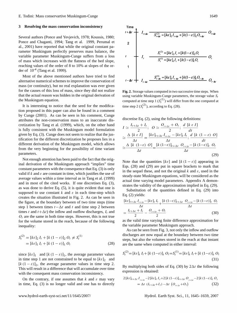
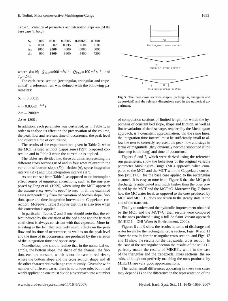
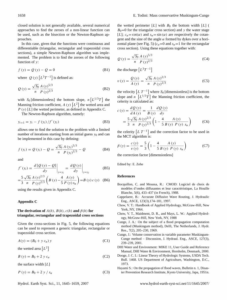