a logistic regression model to predict incident …
TRANSCRIPT

Clemson UniversityTigerPrints
All Theses Theses
12-2009
A LOGISTIC REGRESSION MODEL TOPREDICT INCIDENT SEVERITY USING THEHUMAN FACTORS ANALYSIS ANDCLASSIFICATION SYSTEMHrishikesh KavadeClemson University, [email protected]
Follow this and additional works at: https://tigerprints.clemson.edu/all_theses
Part of the Industrial Engineering Commons
This Thesis is brought to you for free and open access by the Theses at TigerPrints. It has been accepted for inclusion in All Theses by an authorizedadministrator of TigerPrints. For more information, please contact [email protected].
Recommended CitationKavade, Hrishikesh, "A LOGISTIC REGRESSION MODEL TO PREDICT INCIDENT SEVERITY USING THE HUMANFACTORS ANALYSIS AND CLASSIFICATION SYSTEM" (2009). All Theses. 712.https://tigerprints.clemson.edu/all_theses/712

i
A LOGISTIC REGRESSION MODEL TO PREDICT INCIDENT SEVERITY USING THE HUMAN
FACTORS ANALYSIS AND CLASSIFICATION SYSTEM
A Thesis Presented to
the Graduate School of Clemson University
In Partial Fulfillment of the Requirements for the Degree
Master of Science Industrial Engineering
by Hrishikesh Kavade
December 2009
Accepted by: Dr. Anand Gramopadhye, Committee Chair
Dr. Scott Shappell Dr. Paris Stringfellow

ii
ABSTRACT
The Human Factors Analysis and Classification System (HFACS) is a framework
based on Reason’s “Swiss Cheese Theory” and is used to help identify causal factors that
lead to human error. The framework has been used in a variety of industries to identify
leading contributing factors of unsafe events, such as accidents, incidents and near
misses. While traditional application of the HFACS framework to safety outcomes has
allowed evaluators to identify leading causal issues based on frequency, little has been
done to gain a more comprehensive view of the system’s total risk. This work utilizes the
concept of event severity along with the HFACS framework to help better identify target
areas for intervention among unsafe events in wind turbine maintenance.
The objective of this work was to determine if there are any relationships between
the certain HFACS causal factors and an incident’s severity. The analysis was based on
405 cases which were coded for contributing factors using HFACS and were rated for
actual and potential severity using a 10-point severity scale. Models for predicting
potential and actual severity were generated using logistic regression. These models were
then validated using actual data. Although the findings were not significant, it was
determined that decision errors and preconditions to unsafe acts: technological
environment were major contributors to events with high potential severity.
One limitation of this work was the limited availability of complete data on which
to conduct the analysis. So, while the analysis produced non-significance, it is anticipated
that as more data becomes available, the models will yield more concrete findings.
Regardless, understanding the relationships among incident causal factors and outcomes

iii
may shed light on those causal factors which have the potential to lead to catastrophic
events and those which may lead to less severe events.

iv
DEDICATION
I dedicate this thesis to my family.

v
ACKNOWLEDGMENTS
I would like to thank Dr. Gramopadhye for presenting me with this opportunity. I
would also like to thank Dr. Shappell and Dr. Stringfellow for their constant support and
guidance.
vi
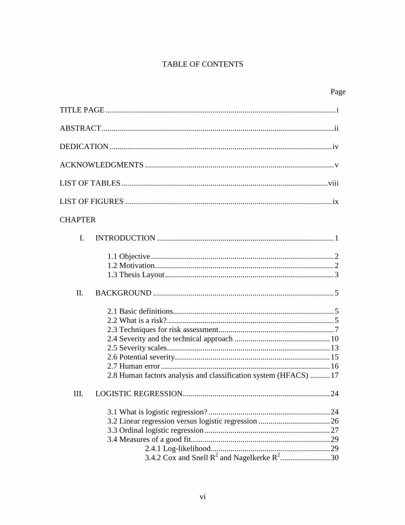
TABLE OF CONTENTS
Page
TITLE PAGE .................................................................................................................... i ABSTRACT ..................................................................................................................... ii DEDICATION ................................................................................................................ iv ACKNOWLEDGMENTS ............................................................................................... v LIST OF TABLES ........................................................................................................ viii LIST OF FIGURES ........................................................................................................ ix CHAPTER I. INTRODUCTION ......................................................................................... 1 1.1 Objective ............................................................................................ 2 1.2 Motivation .......................................................................................... 2 1.3 Thesis Layout ..................................................................................... 3 II. BACKGROUND ........................................................................................... 5 2.1 Basic definitions................................................................................. 5 2.2 What is a risk? .................................................................................... 5 2.3 Techniques for risk assessment .......................................................... 7 2.4 Severity and the technical approach ................................................ 10 2.5 Severity scales .................................................................................. 13 2.6 Potential severity .............................................................................. 15 2.7 Human error ..................................................................................... 16 2.8 Human factors analysis and classification system (HFACS) .......... 17 III. LOGISTIC REGRESSION .......................................................................... 24 3.1 What is logistic regression? ............................................................. 24 3.2 Linear regression versus logistic regression .................................... 26 3.3 Ordinal logistic regression ............................................................... 27 3.4 Measures of a good fit...................................................................... 29 2.4.1 Log-likelihood............................................................ 29 3.4.2 Cox and Snell R2 and Nagelkerke R2 ......................... 30
vii
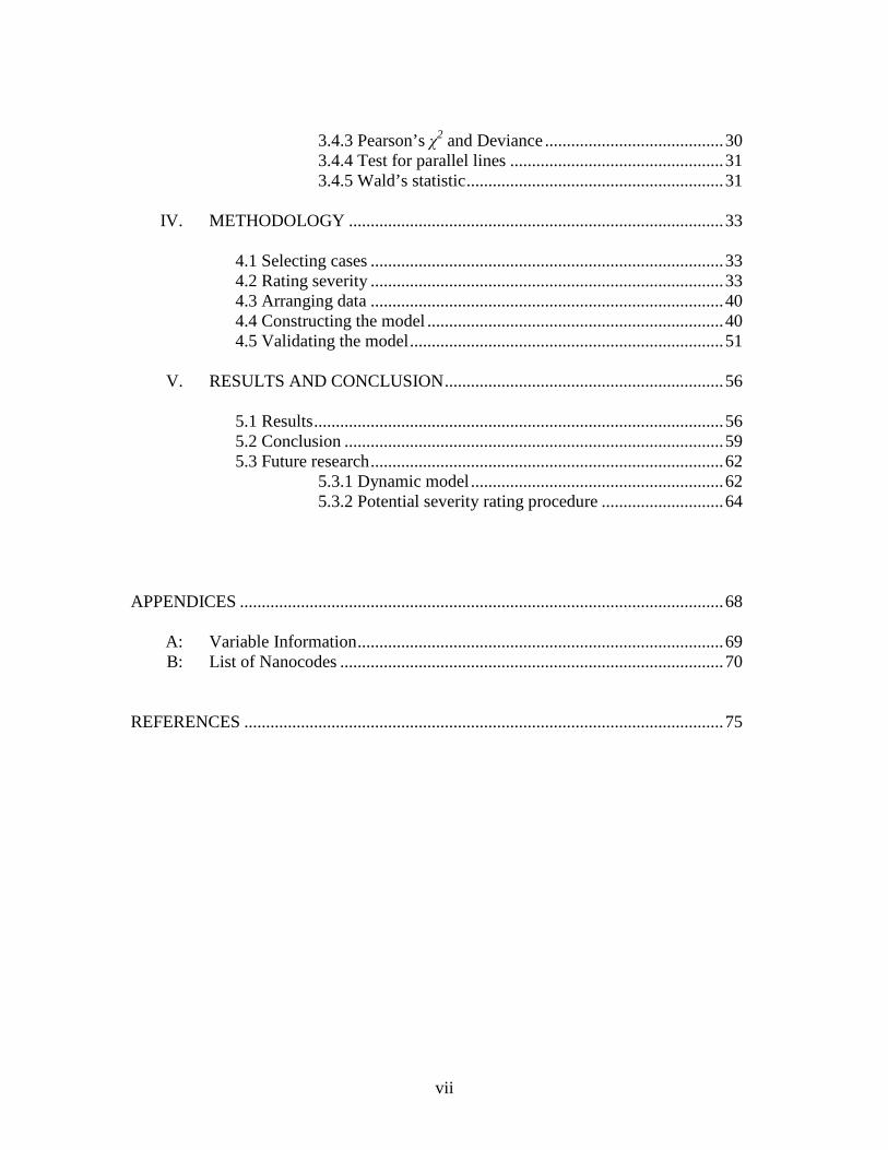
3.4.3 Pearson’s χ2 and Deviance ......................................... 30
3.4.4 Test for parallel lines ................................................. 31 3.4.5 Wald’s statistic ........................................................... 31 IV. METHODOLOGY ...................................................................................... 33 4.1 Selecting cases ................................................................................. 33 4.2 Rating severity ................................................................................. 33 4.3 Arranging data ................................................................................. 40 4.4 Constructing the model .................................................................... 40 4.5 Validating the model ........................................................................ 51 V. RESULTS AND CONCLUSION ................................................................ 56 5.1 Results .............................................................................................. 56 5.2 Conclusion ....................................................................................... 59 5.3 Future research ................................................................................. 62 5.3.1 Dynamic model .......................................................... 62 5.3.2 Potential severity rating procedure ............................ 64 APPENDICES ............................................................................................................... 68 A: Variable Information .................................................................................... 69 B: List of Nanocodes ........................................................................................ 70 REFERENCES .............................................................................................................. 75
viii
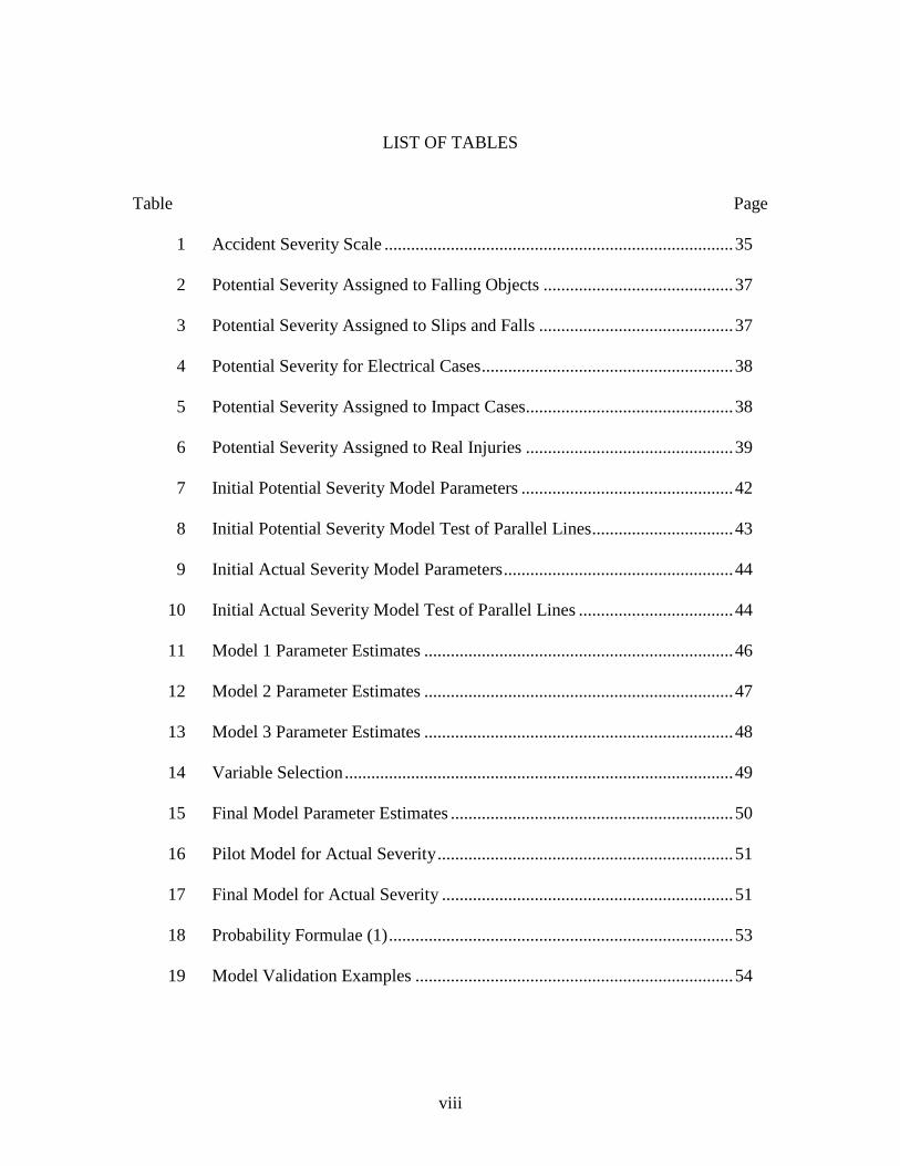
LIST OF TABLES
Table Page 1 Accident Severity Scale ............................................................................... 35 2 Potential Severity Assigned to Falling Objects ........................................... 37 3 Potential Severity Assigned to Slips and Falls ............................................ 37 4 Potential Severity for Electrical Cases ......................................................... 38 5 Potential Severity Assigned to Impact Cases............................................... 38 6 Potential Severity Assigned to Real Injuries ............................................... 39 7 Initial Potential Severity Model Parameters ................................................ 42 8 Initial Potential Severity Model Test of Parallel Lines ................................ 43 9 Initial Actual Severity Model Parameters .................................................... 44 10 Initial Actual Severity Model Test of Parallel Lines ................................... 44 11 Model 1 Parameter Estimates ...................................................................... 46 12 Model 2 Parameter Estimates ...................................................................... 47 13 Model 3 Parameter Estimates ...................................................................... 48 14 Variable Selection ........................................................................................ 49 15 Final Model Parameter Estimates ................................................................ 50 16 Pilot Model for Actual Severity ................................................................... 51 17 Final Model for Actual Severity .................................................................. 51 18 Probability Formulae (1) .............................................................................. 53 19 Model Validation Examples ........................................................................ 54

ix
List of Tables (Continued) Table Page 20 Probability Formulae (2) .............................................................................. 55 21 Model Fitting Information (Final Model) ................................................... 58 22 Goodness-of-fit (Final Model) .................................................................... 58 23 Test of Parallel Lines (Final Model) ........................................................... 58 24 Final Model Summary ................................................................................ 58 25 Omnibus Tests of Final Model Parameters ................................................. 58
x
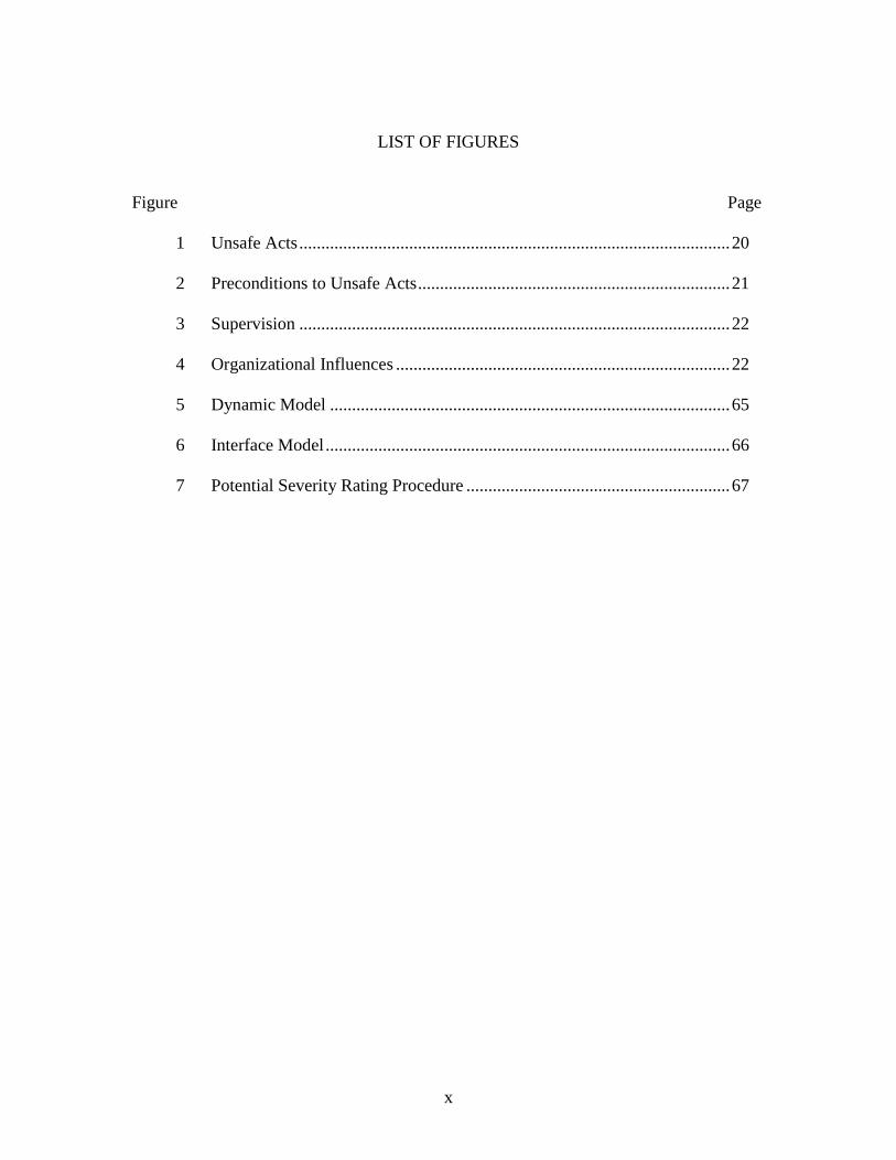
LIST OF FIGURES
Figure Page 1 Unsafe Acts .................................................................................................. 20 2 Preconditions to Unsafe Acts ....................................................................... 21 3 Supervision .................................................................................................. 22 4 Organizational Influences ............................................................................ 22 5 Dynamic Model ........................................................................................... 65 6 Interface Model ............................................................................................ 66 7 Potential Severity Rating Procedure ............................................................ 67

1
CHAPTER ONE
INTRODUCTION
Whether determining which stock to sell to achieve the greatest financial reward
or deciding where to focus this year’s budget for the purchase of safety equipment for
your workforce, Risk Management (RM) is a practice adopted by many both formally
and informally. With regards to industrial safety, RM is a refined discipline and generally
considers the identification, assessment and prioritization of hazards and their
consequences in an effort to strategically and effectively minimize the risk through the
introduction of certain interventions. As such, effective RM does not just address the
resulting outcome, like number of lacerations among a given population, but rather aims
to address the “root cause(s)” which ultimately contributed to the outcome.
One way of helping to identify the “root causes” or contributing causal factors of
an unsafe event is by using the Human Factors Analysis and Classification System
(HFACS). This framework has been used successfully by a number of industries to
identify common latent causal factors in the organizations’ safety performance. Most
often, incident and accident cases are reviewed and classified using the HFACS
framework only to generate an overall list of the most frequently occurring causal factors
(both active and latent). While targeting interventions toward these high-frequency causal
factors may prove effective, using this method there is no way to distinguish between the
magnitude of each event. For instance, the highest occurring causal factor may be a skill-
based error in the form of slips, trips, or falls. As a result, resources may be diverted and
allocated to addressing this single issue. However, further analysis reveals that the

2
severity or consequences of these slips, trips, or falls are minimal and are only resulting
in minor scrapes and bruises. Meanwhile, other less frequent but more catastrophic events
go un-noticed simply due to the low frequency of occurrence. This example highlights
the need to incorporate another parameter, incident severity, into the evaluation process
which will 1) provide a more detailed picture of safety performance in an organization
and 2) enable managers to better identify target areas for intervention.
It is anticipated that certain levels of incident severity are generally influenced by
a common set of similar active and latent causal factors (according to the HFACS
framework). The question becomes, what causal factors are common to high-severity
incidents, medium-severity incidents, and low-severity incidents? And, can we predict
the severity of an incident given an existing set of causal factors?
1.1 Objective
The objective of this thesis is to develop a predictive model for determining the
actual and potential severity of a future incident as a function of existing HFACS causal
factors.
1.2 Motivation
This model should be developed for the following reasons:
1) Future high severity accidents can be prevented by identifying and fixing root causes.

3
2) A standard methodology can be developed which fully utilizes the potential of HFACS in
order to develop probabilistic models. In the literature so far, this approach has not been
taken.
3) Management decisions can be aided by determining the causal categories which attribute
to an increase in probability of high severity. Efforts can thus be directed towards fixing
causes which result in higher severity incidents. Having statistically significant causal
factors makes decision makers trust the means to fix them.
4) The overlooked near accident cases can be fully utilized. Most incident reports have
higher proportion of near accident cases than actual accidents. Authors so far have only
considered actual severity for developing prediction models, which is based on accidents.
Also, there have not been any established procedures that help rate potential severity. A
basic framework for rating potential severity will be established.
1.3 Thesis Layout
The first chapter will begin with some basic definitions and terminologies. This
will be followed by a discussion on the topic of risk and risk assessment. The theory of
human error will be discussed briefly. There will be discussions on the topic of severity.
Then, the Human Factors Analysis and Classification System (HFACS) will be reviewed.
These will be the human factors components used in this study. Mathematical tools have
been used for determining the relationship between causal factors and incident severity in
this study. Hence, logistic regression techniques and the various terminologies associated
with them will be discussed in chapter three.

4
The methodology that will be used for this study will be discussed in detail in the
next chapter. The methodology section will include all the stages in which this study was
conducted, with details of each. The last chapter is results and conclusion, where the
results of this study will be presented. Also, limitations of this study and future research
will be discussed.

5
CHAPTER TWO
BACKGROUND
In this chapter, some basic definitions and terminologies related to accident
investigation and safety engineering will be discussed.
2.1 Basic Definitions
In his work for measuring accident severity, Davidson (2004) has compiled the
following definitions of important terms in safety:
Accident: “An undesired event that results in harm to people, damage to property
or loss to process. It is usually the result of a contact with a substance or a source of
energy above the threshold limit of the body or structure.”(Bird & Germain, 1989, p.36)
Near accident: “An event which, under slightly different circumstances would
have resulted in harm to people, damage to property, or loss to process.” (Bird &
Germain, 1989, p.36)
Incident: An incident comprises of an accident or a near accident. “In a broader
loss control definition, it refers to an event which could or does result in a loss.” (Bird &
Germain, 1989, p.36)
2.2 What is a risk?
The classical definition is that risk (for example, of an accident) is the product of
the probability of that event and (a unified measure of) the (assumed negative)
consequences that necessarily accompany that event (Sheridan, 2008). Other definitions
6
of risk state that, risk is the probability or likelihood of an injury or death (Christensen,
1987). The notion of risk involves both uncertainty and some kind of loss or damage that
might be received (Kaplan & Garrick, 1981). All these definitions formulate risk as
product of probability and consequence or severity. Sheridan (2008) argues that, risk R
with the following formula:
� � �� � ∑ � �|� � � .
In this case, PE is the event probability and the remaining term explains the
consequences of all events that could occur, given that the initial event occurs. Here, Ci is
the consequence.
For an incident E to occur, three other probabilities are taken into account. The
first is the probability of opportunity or exposure to a hazard. The second is attributed to
human error, and takes into account the probability of this error to occur when presented
with the opportunity or exposure. Lastly there is the probability that there is no recovery
to favorable conditions, given the error occurs. Hence, the probability of this unfavorable
outcome is the product of the three probabilities (Sheridan, 2008):
������������� � ������������� � �������|����������� � ���� �������� �� ����|�����
The term ������������� is the term �� used earlier in the definition of risk.
This equation explains the importance of the opportunity or exposure, for an unfavorable
outcome to occur.

7
In the equation for risk R, the term Ci is consequence or severity. There is a
difference between the terms risk, hazard, and uncertainty. As already stated, uncertainty
and damage constitute risk, and uncertainty is just the probability that the desired event
may not occur as planned. Hazard is a source of danger, while risk is the possibility of
loss or injury. Kaplan and Garrick (1981) further theorized a relationship between a risk
and a hazard:
���� � ����� ! "�#�$��� �. This equation states that risk is a ratio of hazards and safeguards. There is always
a small chance of a desired event or activity to have an unfavorable outcome. Thus, risk
can be reduced to an infinitesimal value by increasing safeguards, but never brought
down to zero, because a hazard always exists.
Risk analysis answers the following questions: What can happen? How likely is it
to happen? If it occurs, what are the consequences (Bedford & Cooke, 2001)? The basic
method of risk analysis is the identification and quantification of scenarios, occurrence
probabilities and consequences. Risk, from the context of industrial safety, can be viewed
as a set of scenarios, each with a specific probability of occurrence and quantifiable
impact of consequences (Kaplan & Garrick, 1981). The emphasis here is to model a
specific system (wind turbine maintenance) and construct a mathematical model that
links the accident causation factors and the accident severity. In order to achieve this, it is
important to quantify accident severity.
2.3 Techniques for risk assessment

8
The method to measure risk and categorize risk involves the use of certain
‘first-order’ approaches (Glendon, Clarke, & McKenna, 2006). These are technical,
economic, cultural and psychometric approaches. The technical approach considers risk
as being primarily about seeking safety benefits in such a way that, the acceptable risk
decisions are a matter of correct engineering. In this approach, science is given prime
importance in investigating, analyzing and implementing safety and risk issues. Examples
of this approach include Management Oversight and Risk Tree (MORT) and Failure
Modes and Effects Analysis (FMEA). MORT is fundamentally similar to an event tree.
On the other hand, the economic approach considers the expected benefit, rather than the
harm caused, as the main factor for managing risk. The economic approach considers
hazards as market externalities requiring intervention and social, cultural, political and
anthropological notions are ignored (Viscusi, 1983). Cost-Benefit Analysis (CBA) is an
example of the economic approach.
Cultural theory approach utilizes an anthropological framework for determining
how groups in society interpret hazards and embed trust or distrust in institutions that
create or regulate risk (Douglas, 1992). This is not a quantifiable approach, since it does
not help predict how individuals will behave in their group, which might lead to hazards.
The psychometric approach is based on Risk Perception (RP). RP is considered as a
subjective phenomenon. This approach explains why people perceive hazards differently.
This approach is considered to be the most influential model in the field of risk analysis
by Siegrist, Keller and Kiers (2005). In this study, 26 potential hazards were asked to be
rated not only in terms of severity, also personal factors such as scientific knowledge of

9
the hazard, dread potential, newness and perceived immediacy of effect. This study
aimed to establish that individual perception of a hazard is also an important criterion in
categorizing risk, along with severity and frequency. However, it is difficult to obtain
data regarding the perception that an employee might have about a hazard before an
incident occurs. The data used in our study is compiled from an incident report, and each
and every employee involved in the incident will have to fill in a questionnaire regarding
their perception of the hazard on the basis of the factors described in the study discussed
above. There are various approaches to measure and assess risk. Now, some techniques
for applying these approaches into practice will be discussed.
A risk matrix is a table where columns are represented by probability of an event,
frequency or its likelihood of occurrence, and rows represent an event’s severity, impact
or consequences. Risk is then determined as the product of probability and severity. Risk
is not a measured attribute, but is derived from frequency and severity inputs through a
priori specified formulas such as ���� � &�������� ' "������� (Cox, 2008). Risk
matrices provide a clear framework for analyzing risks. They are easy to construct and
understand. Also, they can easily accommodate for changes to the grid based on specific
applications. On the other hand, it has been argued that, the construction and use of risk
matrices does not need special expertise in the field of risk assessment.
Failure Modes and Effects Analysis (FMEA) is a technique which considers all
the ways by which a system could fail and the consequences that could occur with each
case. Root-cause analysis is used to identify the most responsible cause of the incident
under question. State transition diagrams describe a system as it moves from one state to

10
another, and limits the system to only one state at a time. An event tree describes the
transition of the system from an initiating event to subsequent events. There is a
probability associated with each subsequent event occurring after this initiating event.
According to first order classification by Glendon, Clarke, and McKenna (2006), these
techniques fall into the technical approach. The focus in this study is not only to review
the concept of risk, but also to explore and experiment with the concept of severity. This
study will utilize the technical and the risk perception approaches for developing a
mathematical relationship between causal factors and incident severity.
2.4 Severity and the technical approach
Every occupational accident has a severity associated with it. The severity may be
rated according to damage to an employee’s health, or by cost incurred to the
organization. The severity ratings developed so far take into consideration both these
perspectives.
There are risk matrices which categorize risk according to frequency of an event
and the impact of the event, as argued earlier. Such matrices indicate event probability on
one axis and impact or severity on the other, their product categorizing an event of having
higher risk based on higher impact and probability (Federal Aviation Administration,
2007). Some authors argue that these matrices have poor resolution; typical risk matrices
can correctly and unambiguously compare only less than 10% of randomly selected pairs
of hazards (Cox, 2008). The accuracy in quantifying actual risk is low for risk matrices,
and should be used as an alternative to purely making random decisions. In the risk

11
matrix technique discussed above, the probability of a particular event can be determined
quantitatively based on frequency of the event. Consequence or severity, for example, has
been ‘given’ values between 0 and 1 in the study by Cox (2008). This largely depends on
the analyst’s perception of the impact of the incident. This is where the risk perception
theory comes into play.
Earlier, we discussed FMEA as a technique to analyze risk. FMEA considers the
system in a binary state: pass or fail. It does not consider intermediate degrees by which a
system is damaged, but rather the series of events that lead the system to failure. FMEA
helps investigate all the events leading to a failure, but does not consider how each event
leading to failure is affecting the system in terms of severity. FMEA hence does not
register severity on a continuous basis, but rather on a binary basis.
A state transition probability diagram consists of a large possibility of conditions
that the state of a system can be over time. A state transition diagram also does not
incorporate severity of an incident. Hence, to include severity into these diagrams, one
will have to imagine large number of states emerging from the current, each having a
different severity rating. For example, a system can transition from state A to B with
probability PAB. This new state has a severity s. S can take on a large set of values, and
hence there are a large number of states B with varying values of severity s. Hence,
arguably, state transition probability diagrams can more accurately identify the risk of
potential incidences than the FMEA technique. The same argument can be made for
event trees. Event trees are used primarily, to determine the root cause of an incident,
rather than help determine scenarios with varying severity. In the work by Ross (1981), a

12
serious injury fault tree has been constructed to trace the path of events that lead to a
serious injury. This is like an event tree, but focusing on only serious injuries. Ross
retraces the path of a serious injury from the time of occurrence backwards. He concludes
that a designated activity occurs with inadequate operator actions and unfavorable energy
flow. The above technical approaches help analyze and classify the causes of incidents
and their severity.
Currently, researchers have developed several probabilistic models to predict
severity, given the potential causal factors. This approach for predicting the severity is
based on the variables involved and a probabilistic model is developed. Li and Bai
(2008) have developed a severity predicting model for motorcycle accidents. They
propose a Crash Severity Index (CSI), which is the likelihood that a fatality will occur
given a severe crash occurs. This index can take values between 0 and 1, and is
determined statistically from the work zone variables. The closer the number is to 1, the
higher the possible severity of injury. In a similar study by Dissanayake and Lu (2002)
probabilistic models have been used to predict severity. Automobile crash severity in this
study, has been categorized into five levels: No injury, possible Injury, non-incapacitating
injury, incapacitating injury and fatal injury. The models developed calculate the
probability of occurrence of an injury with a particular level of severity. This can be
better formulated as: Probability [An incident that occurs has a particular severity level].
For example, a model has been developed in this study to calculate the probability of an
incapacitating injury to occur. These models calculate the probability that a higher
severity incident occurs, given that a lesser severity incident has occurred. For example,
13
if a motorcyclist suffers a serious injury, what is the probability that the injury will be
fatal?
2.5 Severity Scales
Lin, Hwang, and Kuo (2008) have reviewed various medical severity scales. The
Injury Severity Scale (ISS) and the Abbreviated Injury Scale (AIS) are used by healthcare
professionals to categorize the trauma faced by their patients (Copes, Sacco, Champion,
& Bain, 1989). The most common scale is the ISS. AIS uses nine body regions to better
summarize injury severity caused by multiple injuries. The ISS uses only six body
regions, instead of nine (Baker, O’Neill, Haddon, & Long, 1974). The ISS scores are
based on the sum of squares of the highest AIS scores for the top three most severely hurt
body parts. The ISS scores range from 1 to 75. New Injury Severity Score (NISS) uses
three most severe injuries independent of whether all three occur in the same region, to
compute the sum of squares (Osler, Baker, & Long, 1997). These scales, however, lack
the sensitivity to accurately classify less severe injuries (Lin, Hwang, & Kuo, 2008).
Based on the part of the body injured and type of injury, physicians can accurately
quantify trauma. Trauma for physicians is analogous to severity for safety engineers.
When considering a severity scale, management is interested in determining how
the severity of the injury will impact the company financially. This may be a combination
of production time lost, worker compensation claims, and equipment damaged. This is
the reason why scales which classify only worker injury trauma; such as an AIS or ISS
cannot be directly used to reflect cost to management.
14
A major power generation company has a severity scale which considers injuries
based on workdays lost. This is 10 point scale with severity increasing from 1 to 10. The
number of workdays lost has been estimated for each serious severity rating. Critical
severity ratings 8, 9 and 10 represent permanent disability, fatality and multiple fatalities,
respectively. Further, two types of severities have been used: potential and actual.
Based on the seriousness of the injury, the incident may result in significant
financial loss to an organization. Many examples of the magnitude of financial loss have
been reviewed by Asfahl (2005). In one example, the average total cost per worker
fatality has been estimated as $790,000 (National Safety Council, 1996). The cost to the
U.S.A.F. for a worker fatality has been estimated as $1,100,000 (U.S. Air Force, 1995).
The costs mentioned above include the compensation, equipment and investigation costs.
The U.S. Department of Energy estimates a loss of $1 million per employee fatality
(Briscoe, 1982). Reportable injuries cost, on an average, $2000 per incident, while a cost
of $1000 per day lost also has been estimated (Crites, 1995). The estimation of these
costs comes from the legal and financial paradigm of safety based on the severity of the
incident (Asfahl, 2005). Hence, the degree by which severity increases according to
financial loss depends on the injury sustained. Severity scales should show the types of
injuries, equipment damaged and the corresponding financial loss.
Sensitivity of a severity scale depends upon the application for which it is to be
used. A mining environment, for example, will employ a ten-point scale for the variety of
medium and serious injuries such as bruises, amputations and electrical shocks. On the
other hand, a severity scale used for assessing injury to computer programmers may use a
15
less sensitive scale targeted for specific injuries. Hence, a severity scale is environment
and work specific, and also has the subjective input of the severity rater. Severity has so
far been quantified by experts and analysts based on their experience and the
environmental inputs. The Accident Frequency-Severity Chart (AFSC) developed by
Priest (1996) enables severity to be rated according to the type of injuries, financial loss
based on injuries and damaged equipment, on the same scale. This scale has been
developed for high risk outdoor activities. Higher numbers on the scale indicate higher
degrees of loss. Priest (1996) suggests that the acceptability of these ratings should be
decided by a committee of experienced personnel in this field; however, these may be
done individually.
2.6 Potential Severity
The discussed severity scales measure the severity of accidents. Injuries need to
occur before cases are rated for severity. There are near accident cases where individuals
could have sustained serious injuries, but were spared from injury by a very small
margin. There will be a severity associated with near accidents if they become accidents.
The situation in which a near accident occurs could result in a major accident in the
future. Potential severity is the subjective severity rating given to potential losses caused
by near accidents. The potential losses can be in the form of physical injury, cost of
damaged equipment or similar degrees of loss. Hence, these situations must be analyzed
in order to determine the causal factors of near accidents.
16
The concerns that needed to be addressed while rating potential severity included:
How can we assign a particular type of injury to a particular situation? For example, how
can we know what type of injury could occur if an object strikes an employee in the head
with considerable force and velocity? Currently, there is no established procedure for
rating potential severity. The ratings are given according to the rater’s subjective view
(Davidson, 2004). A physician can imagine the types of injuries that could occur if near
accidents become accidents. A safety expert can judge the environmental and mental
conditions that most likely result in an accident. A manager can estimate the cost
incurred if the incident occurs. An employee can be trained to describe the situation as
accurately as possible. Each near accident should then be reviewed by all four individuals
and a consensus reached on a potential severity rating. This should be the approach for
rating incidences for potential severity.
2.7 Human Error
Human error has been defined as an inappropriate or undesirable human decision
or behavior that reduces, or has the potential of reducing, effectiveness, safety or system
performance (Sanders & McCormick, 1992). Some actions that can be attributed to
human error would be viewed as appropriate in some systems, until they cause an
incident and the mistake is discovered (Rasmussen, 1979). Another thought is that, an
action might become an error only because the action is performed in an unkind
environment that does not permit detection and reversal of the behavior before an
unacceptable consequence occurs (Rasmussen, 1982). Human Error can then be defined

17
as an action that fails to meet some implicit or explicit criterion (Sheridan, 2008). 70 to
80 percent of all accidents in aviation occur, at least partly, due to human error.
(Shappell & Wiegmann, 1996).
Human error has been classified according to type, such as errors of commission,
omission, sensing, remembering, deciding and responding (Sheridan, 1992). Errors of
commission are caused by incorrectly performing an act. Errors of omission are caused
when there is a failure to do something. A sequence error is caused when a task is
performed out of sequence. A timing error is caused when there is failure to perform a
task within an allotted time period. Further, some authors have classified error based on
how information is processed (Rouse & Rouse, 1983). In this system, errors are identified
as they occur at different stages of information processing. Information processing occurs
in the following stages: Observation of the state of a system, formulating a hypothesis,
testing a hypothesis, choosing a goal, selecting an appropriate procedure and lastly,
execution of the procedure to achieve the goal. When a system is being observed, for
example, there could be incorrect readings of appropriate state variables, or there could
be a failure to observe any state variables at all. Further in the process, there may be
similar errors in hypothesis testing, choice of a goal, choice of a procedure and the
execution of the procedure. The various types of human error have been classified as
causal factors to unfavorable incidences in the HFACS.
2.8 Human Factors Analysis and Classification System (HFACS)

18
The Human Factors Analysis and Classification System (HFACS) has been
developed by Shappell and Wiegmann (2000) in order to methodologically categorize
causes of incidents. A similar approach to HFACS has been to classify errors based on
the type or the level of behavior involved (Rasmussen, 1982). These behaviors have been
classified as skill-based, knowledge-based and rule-based behaviors. Errors in skill-based
behavior are errors in executing an action. Errors in rule-based behavior are errors in
correctly applying preset rules to a situation. Errors in knowledge-based behavior are due
to improper assessment of potential hazards in an unusual situation. An unfavorable
incident occurs when an employee performs an act that is undesirable in that situation,
which leads to injury. However, the reason for this failure to act correctly is more than on
an active level (Reason, 1990). The physical environment, supervision and leadership,
and the organization as a whole, may also be responsible for the employee to perform an
undesired action. For example, the work environment may be too dark for an employee to
perform a given task correctly, which may lead to an accident. Investigating further, one
could find that the supervisor had not updated the employee on the conditions of the work
environment. Further, this investigation could find questionable management policies
responsible.
In light of the different organizational levels of causality, Reason (1990) proposed
that there are active and latent failures. Active failures are apparent, and can be quickly
attributed to have caused the accident. For example, an employee may not be wearing a
mandatory hard-hat, and a head injury occurs. This is the lowest level in the accident
causation structure. On the other hand, latent failures are failures which occur at higher

19
organizational levels, such as the ones in supervision and organizational management.
Latent failures are not apparent at the time of the incident, but come into the spotlight
once an investigation occurs. Reason compared each level to a swiss-cheese slice, with
the holes in the slice corresponding to the failure at each level. The accountability for
each incident can be traced back through the holes in each slice. The failure
accountability goes higher up the organizational hierarchy as holes in higher level swiss-
cheese slices align.
Using this as a reference, HFACS was developed to elaborate on both the active
and latent failures. There are four levels of failure, according to the hierarchy in an
organization. Failure on the lowermost level is attributed to unsafe acts (refer to Fig.1).
Unsafe acts include errors and violations. Decision based errors are errors that an
employee commits due to a consciously thought of action going wrong. For example, an
employee may use improvised tools or equipment in an unusual situation and an injury
occur from this action.
Skill-based errors are caused when an employee performs a task or action with
inadequate skill. For example, an employee may lift an object with improper technique,
causing an injury to the back. Perceptual errors are caused when the auditory or visual
senses do not function correctly due to external influences. For example, an employee
may misjudge the passing clearance under a wire between two electrical poles and cause
an electrical arcing incident. Violations are willful and blatant acts against mandatory
regulations, and may lead to high severity accidents.

20
Fig.1 Unsafe Acts (Shappell & Wiegmann, 2000)
Preconditions to unsafe acts is the causal category which explains the creation of
a hazardous environment which causes an incident (refer to Fig.2). These preconditions
include slippery work surface, temperature and weather conditions. Faulty and non-
functional equipment also constitute a precondition if they are a part of the technological
environment before an incident occurs.
Unsafe leadership is another level of failure further up the organizational
hierarchy (refer to Fig.3). This includes inadequate supervision, planned inappropriate
actions, failure to correct known problem and supervisory violations. All these deal with
substandard supervision practices at the work environment.

21
Fig.2 Preconditions to Unsafe Acts (Shappell & Wiegmann, 2000)

22
Fig.3 Supervison (Shappell & Wiegmann, 2000)
The highest organizational failure is at the senior management level (refer to
Fig.4). The failures at this level are related to poor safety culture as a whole. Failures at
this stage stem from lack of funding, human resources problems such as poor background
checks on employees and other current company policies. Violations at latent levels
result in serious consequences on the management.
Fig.4 Organizational Influences (Shappell & Wiegmann, 2000)

23
The HFACS system hence provides the analyst with a set of all possible causal
factors that can help identify the causes of the incident. The HFACS causal codes will be
used in order to accurately identify causal factors of incidences in the selected work
environment in this study. Organizational influences, precondition to unsafe acts, unsafe
supervision and unsafe acts are called the four levels of failure (Shappell & Wiegmann,
2000). There are three causal categories, resource management, organizational climate
and organizational process. These causal categories have been further divided into
specific causal factors called nanocodes. The specific causes of incidents can be
identified accurately by referring to a list of nanocodes (refer to Appendix B).

24
CHAPTER THREE
LOGISTIC REGRESSION
As discussed earlier, we require specific mathematical tools for developing a model
which relates incident severity and incident causal factors. Hence, logistic regression
techniques and terminologies associated with them will be presented in this chapter.
3.1 What is logistic regression?
Logistic regression is a regression technique employed to fit accident systems.
Logistic regression techniques have been used to model probabilistic systems to predict
future events. These models are direct probability models that have no requirements on
the distributions of the explanatory variables or predictors (Harrell, 2001).
If p is the probability that a binary response variable Y = 1 when input variable X
= x, then the logistic response function is modeled as:
� � ��( � 1|' � * � �+,-+./1 0 �+,-+./
This function represents an s-shaped curve and is non-linear. Here, β is the
coefficient of the predictor or input variable x used in a regression equation. A simplified
version of this function can accommodate for multiple input variables and is linear. This
function is called the logistic regression function and is superior to the logistic response
function (Chatterjee & Hadi, 2006):
� � �1( � 12' � *3, … , '6 � *67 � �+.-+,/,-+8/8-9-+:/:1 0 �+.-+,/,-+8/8-9-+:/:
25
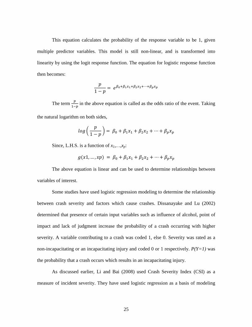
This equation calculates the probability of the response variable to be 1, given
multiple predictor variables. This model is still non-linear, and is transformed into
linearity by using the logit response function. The equation for logistic response function
then becomes:
�1 ; � � �+.-+,/,-+8/8-9-+:/:
The term 63<6 in the above equation is called as the odds ratio of the event. Taking
the natural logarithm on both sides,
=�$ > �1 ; � ? � @A 0 @3*3 0 @B*B 0 9 0 @6*6
Since, L.H.S. is a function of x1,…,xp:
$�*1, … , *� � @A 0 @3*3 0 @B*B 0 9 0 @6*6
The above equation is linear and can be used to determine relationships between
variables of interest.
Some studies have used logistic regression modeling to determine the relationship
between crash severity and factors which cause crashes. Dissanayake and Lu (2002)
determined that presence of certain input variables such as influence of alcohol, point of
impact and lack of judgment increase the probability of a crash occurring with higher
severity. A variable contributing to a crash was coded 1, else 0. Severity was rated as a
non-incapacitating or an incapacitating injury and coded 0 or 1 respectively. P(Y=1) was
the probability that a crash occurs which results in an incapacitating injury.
As discussed earlier, Li and Bai (2008) used Crash Severity Index (CSI) as a
measure of incident severity. They have used logistic regression as a basis of modeling

26
their system. Their approach is similar to that used by Dissanayake and Lu (2002). This
technique has been used to estimate the influences of driver, highway, and environmental
factors on run-off-road crashes (McGinnis, Wissinger, Kelly, & Acuna, 1999). It has
been used to determine the personal and behavioral predictors of automobile crash and
injury severity (Kim, Nitz, Richardson, & Li, 2000). Chang and Yeh (2006) used this
technique to identify the most contributing risk factors for motorcyclist fatalities. In these
studies, the authors have used the environmental and behavioral causes of the incidences
as predictors.
3.2 Linear regression versus logistic regression
In linear regression, the relationship between two variables is in the form of:
( � � 0 @'
In the above equation, � is known as the intercept, or the value of ( when
' � 0. @ is known as the slope or the change in ( when ' increases by one unit. The
method used for estimating the values of � and @ is known as ordinary least-squares
regression (OLS). This method produces the estimates of all the above terms as well as an
error term ej. The error term is the difference between the estimate of ( and ( for case j.
The predicted values of the dependent variable ( are well within the range of possible
values of ( (Menard, 2001). When the dependent variable is dichotomous, it can carry
only two values, 0 or 1. Since the variable is coded in a binary manner, the mean of the
predicted values of the dichotomous variable lies between 0 and 1. Hence, the mean of
this variable can be interpreted as a function of the probability that a selected case will

27
fall into the higher of the two categories for this variable (Menard, 2001). When the
dependent variable is dichotomous and OLS regression is used to estimate the terms, the
predicted values of this dependent variable can exceed 1 or can be less than 0. The values
of probability always lie between 0 and 1, and OLS regression predicts values of the
dependent variable that do not fall in this range.
In logistic regression analysis, the interest is not to directly predict the intrinsic
value of the dependent variable Y but to determine the probability that an event will
occur. Y = 1 indicates that the event has occurred, and P(Y=1) indicates the probability
that it will occur. The problem of having predicted values exceed 1 or be less than zero
can be avoided utilizing the concept of odds ratio discussed earlier. An odds ratio is the
ratio of ( = 1 to ( ≠ 1. For example, if the odds ratio is 1.59, then it indicates that an
observation is 1.59 times more likely to fall in a category Y = 1 than Y = 0. Odds ratios
cannot have values less than zero, but can have values more than one.
Hence, OLS cannot be used to determine the probability that an accident will
occur with a particular level of severity.
3.3 Ordinal logistic regression
The response variable can have more than two ordered levels. The interest may be
to determine the probability that the response will be one of these levels. When there are
three or more ordered categories of the response variable, ordinal logistic regression
(OLR) method is used for modeling (Chatterjee & Hadi, 2006). The dichotomous
dependent variable in binary logistic regression has two levels, 0 and 1. The ordinal

28
response variable has three or more distinct levels increasing in magnitude. An ordered
logit model has the form:
=�$ > �3 1 ; �3 ? � DE 0 @F'
=�$ > �3 0 �B1 ; �3 ; �B ? � DE 0 @F'
.
.
. =�$ > �3 0 �B 0 … 0 �E 1 ; �3 ; �B ; … ; �E ? � DE 0 @F'
OLR is a logistic regression technique that fits two or more regression curves
simultaneously. The equation series above, for example, indicates the odds of belonging
to the group represented by ( = 1 against belonging to the groups represented by ( = 2 to
k. The numbers of equations modeled in this series are the number of ordered categories
minus one. If ( has 3 ordered levels, the number of equations modeled are 2. Each such
equation represents its own logit model, and hence the individual equations are called
logits. The sum of the probabilities from �3 to �E is 1. Hence, OLR models cumulative
probability. One important assumption in modeling with OLR is that, the relation
between independent variables and logits is the same for in all the equations in the series
(Norusis, 2008). The assumption implies that the coefficients of the independent
variables will not vary significantly. Hence, the variable coefficients @F in all the
equations in the series are the same. However, each equation has a different constant term
DE.

29
3.4 Measures of a good fit
3.4.1 Log-likelihood:
Let the log-likelihood of the model with only the constant term be denoted by L0
and the one with the independent variables and the constant term be L1. For binary
logistic regression, the -2 log-likelihood (-2LL) is given by (Menard, 2001):
GA � H��IJ3 =�K��( � 1 L 0 ��IJA =� K��( � 0LM
The -2LL will then be -2 (GA . Here, N are the total number of cases, nY=1
indicates the total number of cases where Y=1. Also, P(Y=1) is nY=1/N. L1 is represented
by the same equation, but the values of the terms will be different due to the inclusion of
independent variables. If the model is fit with the constant term only, it is a subset of the
model with variables. Hence the former model is said to be nested within the latter. The
difference in L0 and L1 when multiplied by -2 is interpreted as a chi-square statistic.
Hence, the difference between the -2LL values of L0 and L1 is interpreted as a chi-square
statistic. However, the models must be nested for the difference to be a chi-square
statistic. This statistic if, if denoted by χ2, is given by:
NB � ;2�GA ; G3
χ2 tests the null hypothesis that the coefficients of the variables in the model are
zero. Hence, if χ2 is statistically significant (p < 0.05), the null hypothesis is rejected.
Rejecting the null hypothesis means that the variables enable the model to make better
predictions than the model without variables. For an ordinal response variable, the same
equations are used, but the difference is the type of event probability. In binary logistic

30
regression, it is P(Y=1), whereas in ordinal the value of 1 is replaced by an ordered
category (Menard, 2001). The values of -2LL should be as small as possible in order for
the model to be a good predictor.
3.4.2 Cox and Snell R2 and Nagelkerke R2
For dichotomous variables, the Cox and Snell R2 and Nagelkerke R2 statistics
provide the geometric mean squared improvement per observation (Menard, 2001).
��* �� "��== �B � 1 ; �PAP3 BQ RSTUVWUXWU YZ � [\ ; >]^]\?ZR_ /K\ ; �]^ ZRL
Here, N are the total number of cases. If the model fits the data perfectly, the
value should be 1, but Cox-Snell R2 statistic does not take this value. The Nagelkerke R2
statistic adjusts the Cox-Snell R2 statistic to take the value of 1. Both statistics are used
for measuring the strength of association between dependent and independent variables.
3.4.3 Pearson’s χ2 and Deviance
For ordinal regression, Pearson’s statistic is used along with Deviance as an
indication of goodness-of-fit. Both values should be small and the significance values
large. The large significance value (p > 0.05) indicates that the null hypothesis is rejected
and the model is a good fit (Norusis, 2008).
All possible dependent variables are cross-tabulated with the independent
variable. A row or column is dedicated for each level of every variable. The frequency of
31
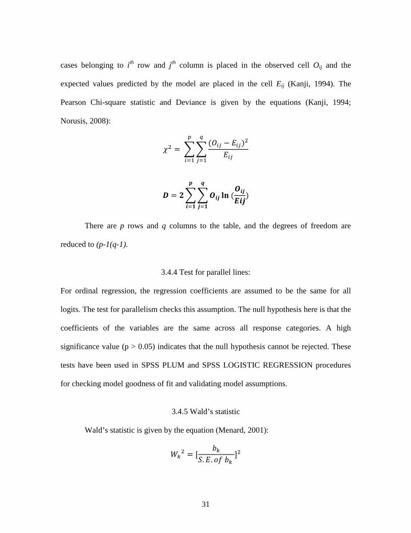
cases belonging to i th row and j th column is placed in the observed cell Oij and the
expected values predicted by the model are placed in the cell Eij (Kanji, 1994). The
Pearson Chi-square statistic and Deviance is given by the equations (Kanji, 1994;
Norusis, 2008):
NB � a a �bc ; �c B�cd
cJ36
J3
] � Z a a efgh
gJ\i
fJ\ jk �efglfg
There are p rows and q columns to the table, and the degrees of freedom are
reduced to (p-1(q-1).
3.4.4 Test for parallel lines:
For ordinal regression, the regression coefficients are assumed to be the same for all
logits. The test for parallelism checks this assumption. The null hypothesis here is that the
coefficients of the variables are the same across all response categories. A high
significance value (p > 0.05) indicates that the null hypothesis cannot be rejected. These
tests have been used in SPSS PLUM and SPSS LOGISTIC REGRESSION procedures
for checking model goodness of fit and validating model assumptions.
3.4.5 Wald’s statistic
Wald’s statistic is given by the equation (Menard, 2001):
mEB � K nE". �. �# nE LB

32
Here, bk is the variable coefficient value and S.E. is the standard error in
estimating the coefficient. This statistic can be distributed asymptotically as a χ2
distribution. Also, it follows standard normal distribution when it is just Wk. This formula
parallels the t-ratio for variable coefficients in OLS. This statistic checks how well each
predictor contributes to the model individually. Hence, a statistically significant Wald’s
statistic for a variable indicates that it should be retained in the model.
Hosmer and Lemeshow (1989) suggest that these significance values should be
set higher than the conventional levels of 0.05 or 0.1 to values such as 0.2 or 0.25. Many
authors (Mickey & Greenland, 1989; Bendel & Afifi, 1977) have used this criterion for
screening variables, since they believe that stricter levels such as p < 0.05 fail to identify
all the important variables. In a study by Dales and Ury (1978), it was determined that
setting significance levels well above the conventional values such as 0.05 or 0.1 reduces
the possibility of a type II error in variable selection.

33
CHAPTER FOUR
METHODOLOGY
The initial chapters laid a foundation for the development of the mathematical
model to relate incident severity and incident causal factors. This chapter will include the
step by step procedure which was used for developing this model. Each sub-procedure
will be discussed before presenting its execution with the given data.
4.1 Selecting cases
The incident report from a power generation company was used as the source of
data. This report has more than five hundred cases. Only incidences related to
maintenance and service activities of the wind turbine generator were considered for
further analysis. Incidences involving a vehicle or occurring off premises were not
considered for further analysis. For the whole data set, 275 of the incidences were
chosen at random using MINITAB software. The remaining 130 the cases were used for
validating the model.
4.2 Rating severity
Each selected case was rated for potential and actual severity. As discussed
earlier, the involved employee, the physician, the engineer and the manager should reach
a consensus while rating potential severity. However, it was not possible to assemble a
team which included the employee involved, the site physician and an on-site safety

34
expert. Hence, for future studies, the suggested methodology can be used. Also, there is
no established procedure for rating severity in the literature so far.
An interesting perspective on assigning severity has been highlighted by
Davidson (2004). Firstly, potential severity ratings were given according to the author’s
subjective view of what could have materialized out of the perceived hazards at that time.
Accident Frequency Severity Chart (AFSC) (Priest, 1996) was used to rate actual
severity. This chart was used as a guiding tool in order to assign a potential severity
rating.
This effective technique was used for rating potential severity in this study. The
AFSC was also used for rating actual severity according to the injuries sustained as
described in the incident report. The increasing magnitude of severity according to injury
type has been shown in the adapted AFSC (refer to table-1). This order was followed
while rating incidences for potential severity. The potential severity was rated for each
case by the author. Potential severity was also rated for the cases where employees had
sustained actual injuries. This was done by increasing the actual severity by one or more
depending on the perceived hazards of the situation as described in the incident report.
The severity was rated based purely on the possible injury sustained by the involved
employee.

35
Table 1- Accident Severity Scale (Priest, 1996; Davidson, 2004):
Severity
Ranking
Injury Impact on
Participation
1 Splinters, insect bites, stings Minor
2 Sunburn, scrapes, bruises, minor cuts
3 Blisters, minor sprain, minor dislocation Cold/heat
stress
4 Lacerations, frostbit, minor burns, mild concussion,
mild hypo/ hyperthermia
Medium
5 Sprains & hyper-extensions, minor fracture
6 Hospital stay < 12 hours fractures, dislocations,
frostbite,
major burn, concussion, surgery, breathing
difficulties,
moderate hypo/ hyperthermia
Major
7 Hospital stay > 12 hours e.g., arterial bleeding,
severe hypo/ hyperthermia, loss of consciousness
8 Major injury requiring hospitalization e.g.,
Spinal damage, head injury
Catastrophic
9 Single death
10 Multiple fatality
36
The incident report included descriptions of the condition in which the incidences
occurred. These included near accidents as well as accidents involving actual injuries.
Many cases in the incident report were already rated for severity. The injury ratings given
for these cases were used to rate for the other cases. For near accidents, the potential
severity was rated by considering the situation where the employee would have been
injured rather than just spared from injury. For example, an employee could be on top of
a three hundred foot high wind turbine tower with inadequate fall protection equipment.
In such a case, potential severity was given according to the worst possible outcome. For
this example, the employee could fall from a height which could prove fatal.
Consistency was maintained while rating cases of similar nature. For example, a
possible fatal fall from 300 feet was always rated as 9, whereas a possible fall of 20 feet
was rated as 6 (Please refer table 1). Cases involving other types of injuries were also
rated in the same manner (refer to tables 2, 3, 4, 5 and 6). The environmental parameters
such as falling height, type of object, electric current voltage were given in the incident
report. However, some cases did not report these important data. For such cases, the
worst possible outcome was assumed.

37
Table 2- Potential severity assigned to falling objects
List of falling objects: Potential Severity: (Falling height one deck 20 feet)
Potential Severity: (Falling height 300 feet)
Wrench 6 9 Phone 4 6 Radio 6 9 Hydraulic torque wrench 6 9 Hammer 6 9 Oil filter and bucket 6 9 Space plate 6 9 Hard case 6 9 Winch nut snap ring 2 4 Unopened soda can 4 6 Crane hook 6 9 Voltmeter 6 9 Latch handle 6 9 Piece of crane boom 6 9 Battery 3 5 Bolt 2 4 Nut 2 4 Slip ring 2 4 Grease gun 6 9
Table 3- Potential severity assigned to slips and falls Description Potential Severity
Fall is from height of 300 feet.
9
Fall is from 20 feet 6
Employee slips and falls on a hard metal surface
6

38
Table 4- Potential severity for electrical cases:
Voltage Potential severity in case of contact with live wire
Potential severity in case of burns sustained from arc flashing
575 9 8 480 9 6 400 9 6 220 9 6 100 8 6 24 4 2
Table 5- Potential severity assigned to impact cases:
Object(s) Part of body Potential Severity Torque wrench Fingers
Brow 6 6
Wrench Toes 6 Hatch, Opening Fingers between 7 Heavy metal parts Fingers between 7 Stepladder, Own weight Fingers between 7 Hydraulic wrench reaction arm, nut, bolt
Fingers between 7
Rotor lock, wrench Fingers between 7 Heavy cable (suspended), ladder rung
Fingers between 7
Mast, nacelle Fingers between 7 Axis cabinet support and rotating gear
Foot 7
Ladder rung Elbow Wrist
7 7
Gearbox Ribs 7 Buss bar Elbow 7 Sledge Hammer Single finger 8 Chisel Knee 7 Hammer Knee
Little finger tip 7 8
Torque multiplier Forearm 7 Hatch Forehead 8

39
Table 6- Potential severity assigned to Real Injuries:
Diagnosed cases: Actual Severity Potential Severity Bursitis in the elbow 6 7 Sprain in the right ring finger
4 5
Laceration to right thumb 5 6 15 mm laceration on his brow
7 8
Contusion to hand and foot Left hand
6 7
Heavy sudden lifting damage to the back
5 6
Laceration to the back of the head
7 8
Laceration wound left leg (grinding wheel)
6 8
Contusion on left maxilla 6 7 Laceration to the head requiring 10 staples
7 8
Laceration requiring three sutures mid cranial back of head
7 8
Laceration to the finger 5 6 Contusion to left ankle 6 7 3 inch laceration on the forehead req. 2 internal and 4 external stitches.
7 8
Fractured Finger, some cuts on the others
7 8
Finger crushed, thumbnail removed
8 8

40
Lastly, the incident report also did not include the financial loss incurred for these
cases. Hence, it was not possible to develop an actual severity scale which incorporated
both physical injury and the cost to the organization. Hence, both the potential and actual
severities were rated based solely on physical injuries.
4.3 Arranging data
MS EXCEL worksheets were used to arrange the preliminary data and assign
causal categories to each case. The original incident report had each case assigned a
causal category according to HFACS methodology. Each selected case had a case ID
assigned in the original incident report. The selected cases with their ID were arranged in
one column. Individual columns were assigned to the 18 causal categories. Columns were
also assigned to potential and actual severity. A 1 was registered in the cell with the row
representing the case ID and column representing the causal category identified for the
case. If two causal factors (nanocodes) of the same causal category were assigned to a
single case, it was only counted once in the corresponding cell. 275 of the cases were
chosen at random using MINITAB. Data from these cases was used for model
construction.
4.4 Constructing the model
There are ten levels by which the actual and potential severities were rated.
Hence, there were two or more ordered levels by which both types of severities could be
rated. There were dichotomous variables representing the causal categories and ordinal

41
variables with more than two levels representing actual and potential severity. Ordinal
logistic regression models determine the probability of an observation to fall into a
specific group, when there are two or more ordered levels of the dependent variable.
Binary logistic regression models calculate the probability of an observation to fall into
one of two groups, when there are two levels of the dependent variable. Hence, it was
suitable to construct the models using ordinal logistic regression. The initial approach
was to construct two ordinal regression models, one with actual severity as the dependent
variable and the other with potential severity. The dependent variables had ten ordered
levels of severity. The initial models included all the contributing variables (refer to
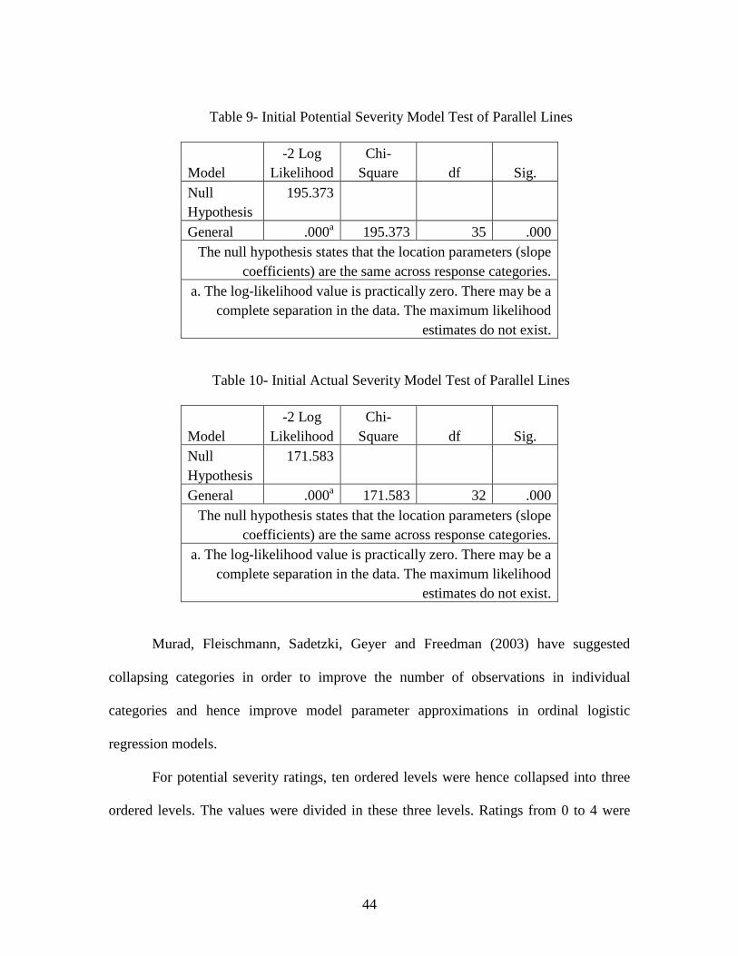
tables 7 and 8). However, none of the models passed the test of parallel lines, which
determines if the variable coefficients are the same for all logits in the ordinal logistic
regression model (refer to tables 9 and 10).

42
Table 7- Initial Potential Severity Model Parameters
Estimate Std. Error Wald df Sig.
95% Confidence Interval Lower Bound Upper Bound
[psev = .00]
-5.141 1.703 9.112 1 .003 -8.479 -1.803
[psev = 3.00]
-1.966 1.400 1.972 1 .160 -4.709 .778
[psev = 4.00]
-.554 1.396 .157 1 .692 -3.291 2.183
[psev = 5.00]
.014 1.398 .000 1 .992 -2.726 2.754
[psev = 6.00]
.654 1.400 .218 1 .641 -2.091 3.398
[psev = 7.00]
1.175 1.402 .703 1 .402 -1.572 3.922
[psev = 8.00]
1.595 1.402 1.294 1 .255 -1.153 4.342
[psev = 9.00]
6.564 1.689 15.098
1 .000 3.253 9.874
[de=.00] .684 .312 4.787 1 .029 .071 1.296 [de=1.00] 0a . . 0 . . . [se=.00] .504 .294 2.939 1 .086 -.072 1.080 [se=1.00] 0a . . 0 . . . [v=.00] -1.823 .590 9.533 1 .002 -2.981 -.666 [v=1.00] 0a . . 0 . . . [pte=.00] .371 .271 1.876 1 .171 -.160 .901 [pte=1.00] 0a . . 0 . . . [f=.00] 1.310 1.039 1.592 1 .207 -.725 3.346 [f=1.00] 0a . . 0 . . .
a. This parameter is set to zero because it is redundant.

43
Table 8- Initial Actual Severity Model Parameters
Estimate Std. Error Wald df Sig.
95% Confidence Interval Lower Bound Upper Bound
[asev = .00]
-3.846 2.367 2.639 1 .104 -8.486 .794
[asev = 1.00]
-2.772 2.359 1.381 1 .240 -7.396 1.851
[asev = 3.00]
-2.000 2.354 .722 1 .395 -6.613 2.612
[asev = 4.00]
-.550 2.356 .054 1 .815 -5.167 4.067
[asev = 5.00]
2.039 2.533 .648 1 .421 -2.925 7.004
[de=.00] -1.248 .335 13.847 1 .000 -1.906 -.591 [de=1.00] 0a . . 0 . . . [se=.00] -.994 .322 9.508 1 .002 -1.626 -.362 [se=1.00] 0a . . 0 . . . [pte=.00] -.529 .293 3.267 1 .071 -1.103 .045 [pte=1.00] 0a . . 0 . . . [f=.00] -1.964 1.050 3.497 1 .061 -4.022 .095 [f=1.00] 0a . . 0 . . . [pe=.00] -2.454 .836 8.620 1 .003 -4.092 -.816 [pe=1.00] 0a . . 0 . . . [ams=.00] 2.109 1.021 4.262 1 .039 .107 4.111 [ams=1.00]
0a . . 0 . . .
[cc=.00] -2.596 .547 22.485 1 .000 -3.669 -1.523 [cc=1.00] 0a . . 0 . . . [is=.00] 2.512 1.443 3.030 1 .082 -.316 5.341 [is=1.00] 0a . . 0 . . .
a. This parameter is set to zero because it is redundant.
44
Table 9- Initial Potential Severity Model Test of Parallel Lines
Model -2 Log
Likelihood Chi-
Square df Sig. Null Hypothesis
195.373
General .000a 195.373 35 .000 The null hypothesis states that the location parameters (slope
coefficients) are the same across response categories. a. The log-likelihood value is practically zero. There may be a
complete separation in the data. The maximum likelihood estimates do not exist.
Table 10- Initial Actual Severity Model Test of Parallel Lines
Model -2 Log
Likelihood Chi-
Square df Sig. Null Hypothesis
171.583
General .000a 171.583 32 .000 The null hypothesis states that the location parameters (slope
coefficients) are the same across response categories. a. The log-likelihood value is practically zero. There may be a
complete separation in the data. The maximum likelihood estimates do not exist.
Murad, Fleischmann, Sadetzki, Geyer and Freedman (2003) have suggested
collapsing categories in order to improve the number of observations in individual
categories and hence improve model parameter approximations in ordinal logistic
regression models.
For potential severity ratings, ten ordered levels were hence collapsed into three
ordered levels. The values were divided in these three levels. Ratings from 0 to 4 were

45
collapsed into the lowermost level. Hence, the ratings from 0 to 4 were coded as 0.
Severity ratings from 5 to 7 were collapsed into the middle level and 8 to 10 in the
highest level. These ratings were coded as 1 and 2 respectively.
There are 18 distinct causal categories. Each category represents an independent
variable used in the model. The variables which did not contribute towards the
occurrence of any incident at all were eliminated from further analysis. These variables
were pml, sv, oc, fcp and pis (refer to Appendix A.).
The remaining variables were selected for fitting in further models. The initial
model for potential severity included all the contributing variables (refer to table-11).
Variables which had their Wald’s statistic significant at a p-value < 0.25 were selected
for fitting in the next model (refer to tables-12 and 13). The procedure continued till all
variables and constants had a significant Wald’s statistic (refer to table- 14). The final
model for potential severity included four causal categories (refer to table- 15). The
models were constructed on SPSS v.17.0. SPSS PLUM ordinal logistic regression
procedure was utilized for fitting the models. For the variables in the final model, two-
way, three-way and four-way interactions were investigated for their contribution to the
model. These interactions were added in the model. There were no cases where five or
more causal categories were identified at once, and hence higher level interaction terms
were not included in the models.

46
Table 11- Model 1 Parameter Estimates
Estimate Std. Error Wald df Sig.
95% Confidence
Interval Lower Bound
Upper Bound
[ordinal1 = .00]
1.121 2.867 .153 1 .696 -4.499 6.741
[ordinal1 = 1.00]
2.847 2.874 .982 1 .322 -2.785 8.480
[de=.00] .834 .353 5.587 1 .018 .142 1.525 [de=1.00] 0a . . 0 . . . [se=.00] .474 .325 2.131 1 .144 -.163 1.111 [se=1.00] 0a . . 0 . . . [pe=.00] .605 .862 .492 1 .483 -1.086 2.295 [pe=1.00] 0a . . 0 . . . [v=.00] -1.690 .668 6.395 1 .011 -3.000 -.380 [v=1.00] 0a . . 0 . . . [ppe=.00] .401 .334 1.442 1 .230 -.253 1.054 [ppe=1.00] 0a . . 0 . . . [pte=.00] .552 .299 3.402 1 .065 -.035 1.138 [pte=1.00] 0a . . 0 . . . [ams=.00] .238 .596 .160 1 .689 -.930 1.407 [ams=1.00] 0a . . 0 . . . [aps=.00] 1.052 1.369 .591 1 .442 -1.631 3.736 [aps=1.00] 0a . . 0 . . . [cc=.00] .479 .551 .756 1 .385 -.600 1.558 [cc=1.00] 0a . . 0 . . [f=.00] 1.198 1.106 1.174 1 .279 -.969 3.366 [f=1.00] 0a . . 0 . . . [is=.00] -1.459 1.035 1.987 1 .159 -3.488 .570 [is=1.00] 0a . . 0 . . [rm=.00] .393 .735 .286 1 .593 -1.048 1.835 [rm=1.00] 0a . . 0 . . . [op=.00] -.171 1.097 .024 1 .876 -2.321 1.978

47
[op=1.00] 0a . . 0 . . .
a. This parameter is set to zero because it is redundant.
Table 12- Model 2 Parameter Estimates
Estimate Std. Error Wald df Sig.
95% Confidence
Interval Lower Bound
Upper Bound
[ordinal1 = .00]
-1.344 1.820 .545 1 .460 -4.910 2.223
[ordinal1 = 1.00]
.372 1.821 .042 1 .838 -3.197 3.942
[de=.00] .806 .339 5.653 1 .017 .142 1.471 [de=1.00] 0a . . 0 . . . [se=.00] .372 .312 1.424 1 .233 -.239 .983 [se=1.00] 0a . . 0 . . . [v=.00] -1.587 .632 6.309 1 .012 -2.826 -.349 [v=1.00] 0a . . 0 . . . [ppe=.00] .365 .329 1.235 1 .266 -.279 1.009 [ppe=1.00] 0a . . 0 . . . [pte=.00] .486 .291 2.779 1 .096 -.085 1.057 [pte=1.00] 0a . . 0 . . . [f=.00] 1.113 1.103 1.019 1 .313 -1.048 3.275 [f=1.00] 0a . . 0 . . . [is=.00] -1.267 1.003 1.596 1 .207 -3.233 .699 [is=1.00] 0a . . 0 . . .
a. This parameter is set to zero because it is redundant.

48
Table 13- Model 3 Parameter Estimates
Estimate Std. Error Wald df Sig.
95% Confidence
Interval Lower Bound
Upper Bound
[ordinal1 = .00]
-2.559 1.362 3.528 1 .060 -5.229 .111
[ordinal1 = 1.00]
-.849 1.358 .391 1 .532 -3.512 1.813
[de=.00] .756 .335 5.075 1 .024 .098 1.413 [de=1.00] 0a . . 0 . . . [se=.00] .337 .309 1.185 1 .276 -.270 .943 [se=1.00] 0a . . 0 . . . [v=.00] -1.629 .631 6.671 1 .010 -2.864 -.393 [v=1.00] 0a . . 0 . . . [ppe=.00] .340 .328 1.076 1 .300 -.302 .982 [ppe=1.00] 0a . . 0 . . . [pte=.00] .472 .291 2.637 1 .104 -.098 1.041 [pte=1.00] 0a . . 0 . . . [is=.00] -1.263 1.002 1.589 1 .207 -3.228 .701 [is=1.00] 0a . . 0 . . .
a. This parameter is set to zero because it is redundant.

49
Table 14- Variable Selection
Variable Model 1 Model 2 Model 3 Final Model
de Included Included Included Included
se Included Included Not-Included Not-Included
pe Included Not-Included Not-Included Not-Included
v Included Included Included Included
ppe Included Included Included Not-Included
pte Included Included Included Included
ams Included Not-Included Not-Included Not-Included
aps Included Not-Included Not-Included Not-Included
pml Not-Included Not-Included Not-Included Not-Included
cc Included Not-Included Not-Included Not-Included
f Included Not-Included Not-Included Not-Included
is Included Included Included Included
pis Not-Included Not-Included Not-Included Not-Included
sv Not-Included Not-Included Not-Included Not-Included
rm Included Not-Included Not-Included Not-Included
oc Not-Included Not-Included Not-Included Not-Included
op Included Not-Included Not-Included Not-Included
fcp Not-Included Not-Included Not-Included Not-Included
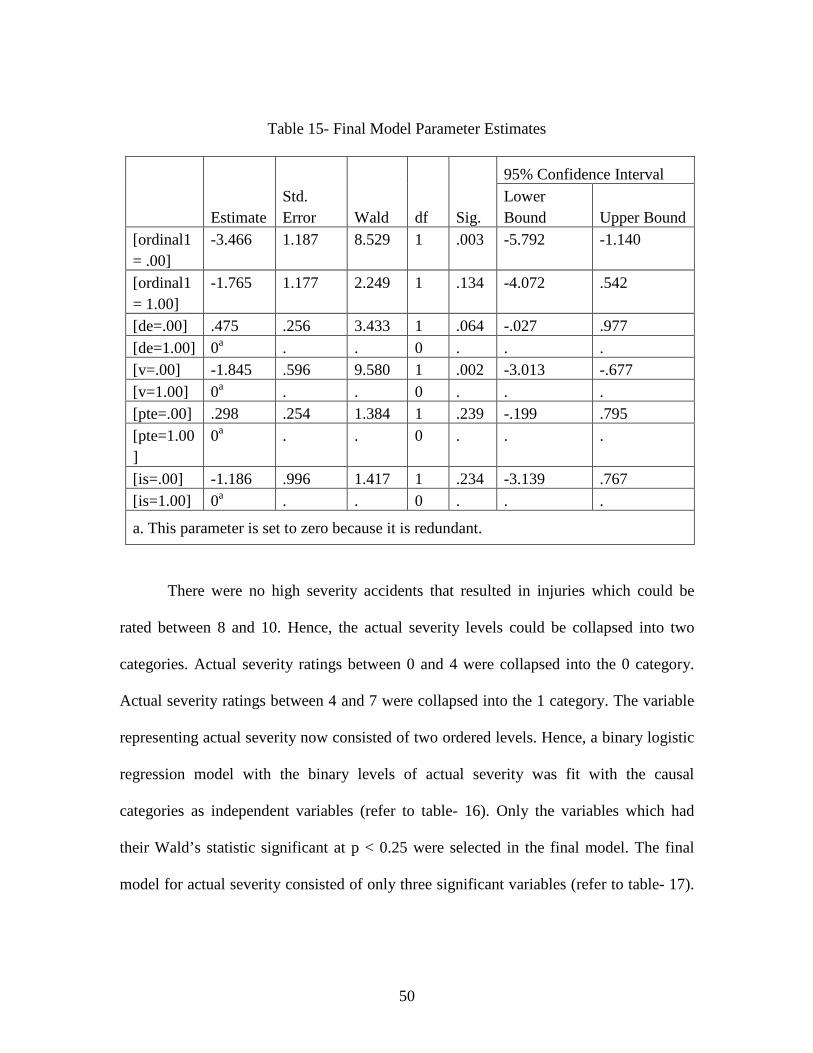
50
Table 15- Final Model Parameter Estimates
Estimate Std. Error Wald df Sig.
95% Confidence Interval Lower Bound Upper Bound
[ordinal1 = .00]
-3.466 1.187 8.529 1 .003 -5.792 -1.140
[ordinal1 = 1.00]
-1.765 1.177 2.249 1 .134 -4.072 .542
[de=.00] .475 .256 3.433 1 .064 -.027 .977 [de=1.00] 0a . . 0 . . . [v=.00] -1.845 .596 9.580 1 .002 -3.013 -.677 [v=1.00] 0a . . 0 . . . [pte=.00] .298 .254 1.384 1 .239 -.199 .795 [pte=1.00]
0a . . 0 . . .
[is=.00] -1.186 .996 1.417 1 .234 -3.139 .767 [is=1.00] 0a . . 0 . . .
a. This parameter is set to zero because it is redundant.
There were no high severity accidents that resulted in injuries which could be
rated between 8 and 10. Hence, the actual severity levels could be collapsed into two
categories. Actual severity ratings between 0 and 4 were collapsed into the 0 category.
Actual severity ratings between 4 and 7 were collapsed into the 1 category. The variable
representing actual severity now consisted of two ordered levels. Hence, a binary logistic
regression model with the binary levels of actual severity was fit with the causal
categories as independent variables (refer to table- 16). Only the variables which had
their Wald’s statistic significant at p < 0.25 were selected in the final model. The final
model for actual severity consisted of only three significant variables (refer to table- 17).
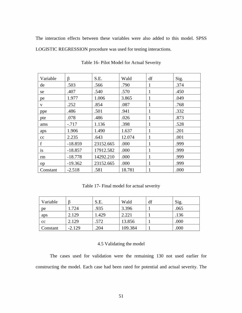
51
The interaction effects between these variables were also added to this model. SPSS
LOGISTIC REGRESSION procedure was used for testing interactions.
Table 16- Pilot Model for Actual Severity
Variable β S.E. Wald df Sig. de .503 .566 .790 1 .374 se .407 .540 .570 1 .450 pe 1.977 1.006 3.865 1 .049 v .252 .854 .087 1 .768 ppe .486 .501 .941 1 .332 pte .078 .486 .026 1 .873 ams -.717 1.136 .398 1 .528 aps 1.906 1.490 1.637 1 .201 cc 2.235 .643 12.074 1 .001 f -18.859 23152.665 .000 1 .999 is -18.857 17912.582 .000 1 .999 rm -18.778 14292.210 .000 1 .999 op -19.362 23152.665 .000 1 .999 Constant -2.518 .581 18.781 1 .000
Table 17- Final model for actual severity
Variable β S.E. Wald df Sig. pe 1.724 .935 3.396 1 .065 aps 2.129 1.429 2.221 1 .136 cc 2.129 .572 13.856 1 .000 Constant -2.129 .204 109.384 1 .000
4.5 Validating the model
The cases used for validation were the remaining 130 not used earlier for
constructing the model. Each case had been rated for potential and actual severity. The

52
probability that a case with given input variables has a particular potential severity rating
was determined using the formulae in table 18 (Norusis, 2008):
Each case where one or more of the variables from the group de, is, pte and v
were identified as causal categories could provide the inputs 0 or 1 for the equations.
Cases where these variables were not identified as causal categories were not selected for
validation, since this meant that the coefficients of all the variables in the equations
would be zero. The eliminated variables have coefficients which are not significant
statistically, and hence do not contribute to the model. Cases were categorized as being
correctly predicted if the calculated probability was above 0.85. For example, (refer to
table- 19) for a particular case, v was identified as a causal category and the severity
rating given belonged in the middle level (potential severity between 5 and 7). The low
probability calculated (0.35, <0.85) classified this case as not correctly predicted.

53
Table 18- Probability Formulae(1) Probability Formula P(severity of an incident will be in a specific category j)
� >�������� �# �o� ���� ��� p�== n� �� ����$����� =��� �o�� �� ����= �� q ?; ���������� �# �o� ���� ��� p�== n� �� ����$����� =��� �o�� q
P(severity of an incident will be in categories less than and equal to j)
11 0 �<�rs<+/ t
P (severity of incident will be between 0-4)
11 0 �<K�<u.vww <A.vxyz{-3.|vy}<A.B~|6�{-3.3|w� L
P (severity of incident will be between 5-7)
K 11 0 �<K�<3.xwy <A.vxyz{-3.|vy}<A.B~|6�{-3.3|w� L; 11 0 �<K�<u.vww <A.vxyz{-3.|vy}<A.B~|6�{-3.3|w� LL
P (severity of incident will be between 8-10)
1 ; 11 0 �<K�<3.xwy <A.vxyz{-3.|vy}<A.B~|6�{-3.3|w� L
* αj : Constant value in for the categories j @ : Variable coefficient x : Variable value (Either 1 or 0). Variables were de, v, pte and is.

54
Table 19- Model validation examples:
Case Given
potential
Severity
rating
Collapsed
potential
Severity
group
Given
Ordinal
category
Predicted probability that
severity will
be between
Correctly
Predicted?
0-4 5-7 8-10
1 4 0-4 0 0.165 0.355 0.480 No
2 8 8-10 2 0.02 0.077 0.903 Yes
In another case, the causal category de and severity rating belonging highest level
(severity between 8 and 10) was given. The high calculated probability value (0.903, >
0.85) classified this case as being correctly predicted for potential severity.
For the actual severity model the probability of belonging to the highest group
(probability of severity between 4 and 7) was calculated using the equation in table- 20
(Menard, 2001). The procedure used for the validation of the potential severity model
was also applied for validating the actual severity model.

55
Table 20- Probability Formulae (2)
General Formula
��( � 1 � �r- +,�,-+,�,-9- +��� 1 0 �r- +,�,-+,�,-9- +��� P(severity of
incident will be
between 4 and 7)
��( � 1 � �<B.3B~- 3.xBv6{-B.3B~�6� - B.3B~�� 1 0 �<B.3B~- 3.xBv6{-B.3B~�6� - B.3B~��
P(severity of an
incident will be
between 0 and 3)
��( � 0 � 1 ; �<B.3B~- 3.xBv6{-B.3B~�6� - B.3B~�� 1 0 �<B.3B~- 3.xBv6{-B.3B~�6� - B.3B~��
* α : Constant value @ : Variable coefficient x : Variable value (Either 1 or 0). Variables were pe, aps and cc.

56
CHAPTER FIVE
RESULTS AND CONCLUSION
In this section, the results of this study will be presented along with its limitations.
Future works will be discussed based on the lessons learnt from this study.
5.1 Results
The various measures of model fitting discussed earlier were used as indicators of
how well a model fits the data. The final potential severity model had four variables
(refer to table- 14). Each variable had statistically significant Wald’s statistics. The test
for common slopes was statistically insignificant (p>0.05). Hence, the null hypothesis
that the coefficients of the variables are the same across all the logits could not be
rejected (refer to table- 23). The intercept (constant) values for both the logits showed
statistically significant Wald’s statistics at a p-value of 0.25. Also, the Pearson Chi-
square and Deviance Chi-square values are statistically insignificant at a p-value of 0.05
(refer to table- 22). The null hypothesis that the model does not fit is rejected, and model
is a good fit with the chosen variables (refer to table- 21). In the validation stage, it was
determined that the potential severity model could predict 35% of the validation cases
correctly. However, the model correctly predicted 87% of the cases whose severity was
between 8 and 10. Hence, this model can be utilized to determine the probability of high
potential severity for incidents.
The variables included in the final model for potential severity were decision
error, violation, preconditions to unsafe acts: technological environment and inadequate
supervision. Decision Error and preconditions to unsafe acts: technological environment
57
need to be investigated and safety interventions targeted in order to prevent high potential
severity incidents in the future. These variable coefficients are positive, and hence the
presence of these two causal categories increases the probability of an incident occurring
with higher potential severity (refer to table- 15).
For the final actual severity model, all three selected variables had Wald’s
statistics statistically significant at a p-value of 0.25 (refer to table- 17). The likelihood
ratio chi-square statistic has a p-value < 0.05. Hence, the hypothesis that model variable
coefficients are zero can be rejected, and the model with the variables fits significantly
better than the model without the variables (refer to table- 25). The high -2LL value
indicates that the model fits the data poorly and the low Cox and Snell and Nagelkerke R2
statistic values indicate a small improvement per observation from the null model (refer
to table- 24). The actual severity model could not correctly predict the probability of
belonging to the higher group (probability of severity between 4 and 7) or the lower
group (probability of severity between 0 and 3) for any of the validation cases. The cutoff
here was also 0.85, as assumed in the case of potential severity models. Hence, the actual
severity model cannot be used for predicting the actual severity of incidents. More
incidences need to be reported and the model re-fitted.
There were no interaction terms whose Wald’s statistics were found to be
statistically significant at a p < 0.25 level, for both the actual and potential severity
models. Hence these models only included the main effects.

58
Table 21- Model Fitting Information (Final Model)
Model -2 Log Likelihood
Chi-Square df Sig.
Intercept Only
69.429
Final 48.088 21.341 4 .000
Table 22- Goodness-of-fit (Final Model)
Chi-Square df Sig.
Pearson 9.869 12 .627
Deviance 11.461 12 .490
Table 23- Test of Parallel Lines (Final Model)
Model -2 Log Likelihood
Chi-Square df Sig.
Null Hypothesis
48.088
General 44.233 3.855 4 .426
Table 24- Final Model Summary:
-2 Log likelihood Cox & Snell R Square
Nagelkerke R Square
200.974a .057 .105
Table 25- Omnibus tests of final model parameters:
Chi-square df Sig. Step 16.241 3 .001 Block 16.241 3 .001 Model 16.241 3 .001
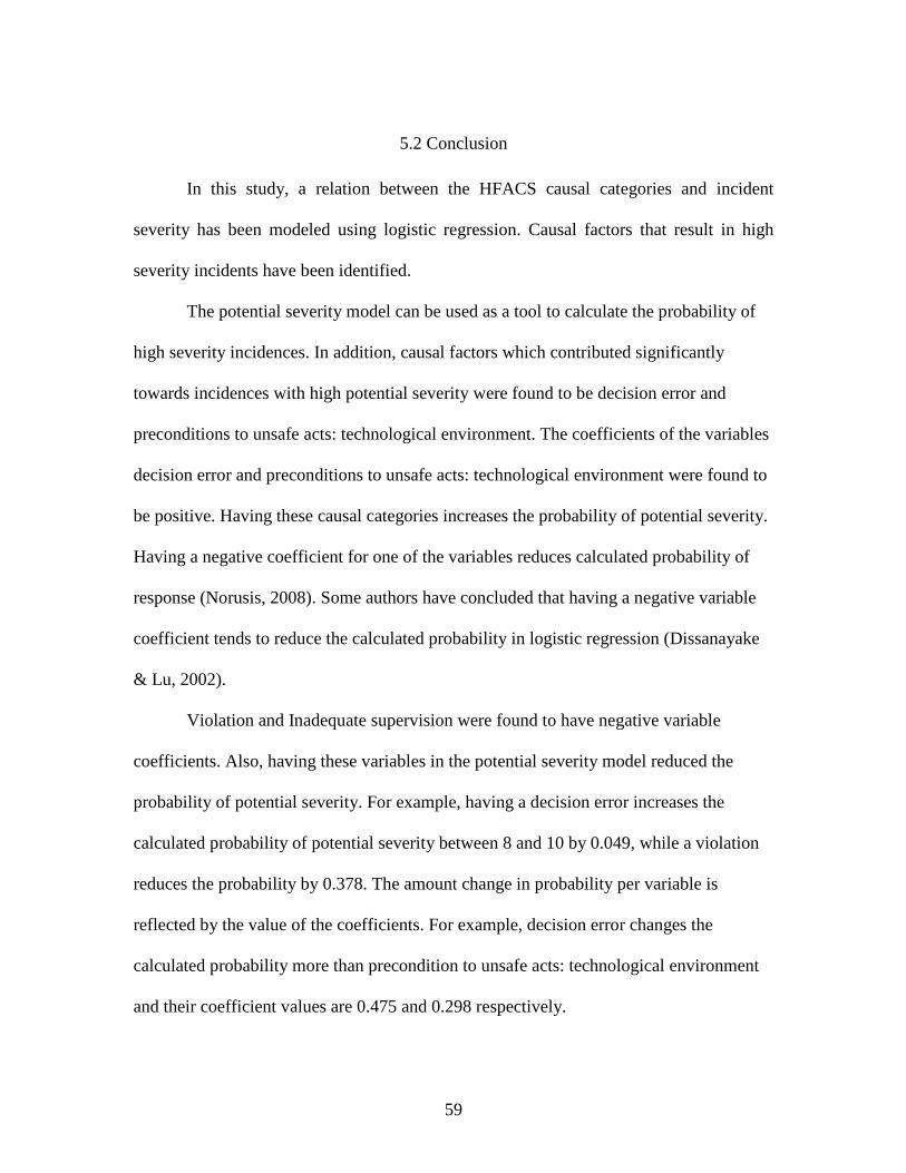
59
5.2 Conclusion
In this study, a relation between the HFACS causal categories and incident
severity has been modeled using logistic regression. Causal factors that result in high
severity incidents have been identified.
The potential severity model can be used as a tool to calculate the probability of
high severity incidences. In addition, causal factors which contributed significantly
towards incidences with high potential severity were found to be decision error and
preconditions to unsafe acts: technological environment. The coefficients of the variables
decision error and preconditions to unsafe acts: technological environment were found to
be positive. Having these causal categories increases the probability of potential severity.
Having a negative coefficient for one of the variables reduces calculated probability of
response (Norusis, 2008). Some authors have concluded that having a negative variable
coefficient tends to reduce the calculated probability in logistic regression (Dissanayake
& Lu, 2002).
Violation and Inadequate supervision were found to have negative variable
coefficients. Also, having these variables in the potential severity model reduced the
probability of potential severity. For example, having a decision error increases the
calculated probability of potential severity between 8 and 10 by 0.049, while a violation
reduces the probability by 0.378. The amount change in probability per variable is
reflected by the value of the coefficients. For example, decision error changes the
calculated probability more than precondition to unsafe acts: technological environment
and their coefficient values are 0.475 and 0.298 respectively.
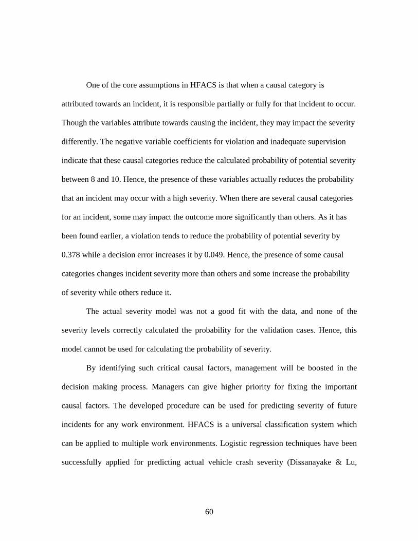
60
One of the core assumptions in HFACS is that when a causal category is
attributed towards an incident, it is responsible partially or fully for that incident to occur.
Though the variables attribute towards causing the incident, they may impact the severity
differently. The negative variable coefficients for violation and inadequate supervision
indicate that these causal categories reduce the calculated probability of potential severity
between 8 and 10. Hence, the presence of these variables actually reduces the probability
that an incident may occur with a high severity. When there are several causal categories
for an incident, some may impact the outcome more significantly than others. As it has
been found earlier, a violation tends to reduce the probability of potential severity by
0.378 while a decision error increases it by 0.049. Hence, the presence of some causal
categories changes incident severity more than others and some increase the probability
of severity while others reduce it.
The actual severity model was not a good fit with the data, and none of the
severity levels correctly calculated the probability for the validation cases. Hence, this
model cannot be used for calculating the probability of severity.
By identifying such critical causal factors, management will be boosted in the
decision making process. Managers can give higher priority for fixing the important
causal factors. The developed procedure can be used for predicting severity of future
incidents for any work environment. HFACS is a universal classification system which
can be applied to multiple work environments. Logistic regression techniques have been
successfully applied for predicting actual vehicle crash severity (Dissanayake & Lu,

61
2002; Li & Bai, 2008) and also in determining causal factors that lead to high severity
incidents in coal mines (Maiti & Bhattacherjee, 1999). The work done in this thesis also
extends this application to wind turbine generator maintenance activities. In addition, the
HFACS system has been used successfully in conjunction with the concept of potential
severity.
One of the drawbacks in using logistic regression is that, data from previous cases
is required for modeling. Hence, a large number of incidences need to occur in the
environment of interest in order to construct the model. Also, probability of severity
cannot be determined for incidences with causal categories are not represented by the
variables in the final models. Further, the criterion used in variable selection of p < 0.25,
though supported by previous work in this field (Mickey & Greenland, 1989), will be
doubted by researchers who utilize the traditional value of 0.05.
When new incidents are added to the report, the data changes and hence, new
models need to be fit for the new data. Hence, the next step is to develop an application
which works on a dynamic level by fitting new models automatically and immediately
when the incident report changes. Secondly, the severity rated by a physician in
conjunction with a safety engineer and the involved employee would be more accurate in
terms of damage sustained to the human body and the potential environmental hazards.
Hence, in future studies, both types of severities need to be rated for each case with the
consent of all involved personnel. There has not been an established procedure to rate
potential severity. These drawbacks can be eliminated by developing new techniques
which can be used for similar studies in the future.

62
5.3 Future research
5.3.1 Dynamic model
Once the model is validated using the methodology presented in this paper, it can
be used for making future predictions. However, if new incidences occur, the data in the
incident report changes and hence new models need to be fit. A constant revision of data
should also trigger a constant revision of the model fitting process. This process is shown
in the flowchart below (refer to Fig. 5):
Fig. 5 Dynamic Model

63
When the database is modified, a trigger starts the methodology for fitting the
model as discussed in this study. A change in the incident report triggers the statistical
software to follow the model fitting methodology. If the models are a good fit, the
validation program is triggered. Otherwise, random samples are chosen till the model fits
satisfactorily. The output can then be interpreted by the user. Hence, the next step is the
development of a dynamic model where new changes in the incident report trigger a
series of programs which fit new models.
Also, once the model had been validated, an interface can be developed which
returns the severity probability once the user inputs causal categories. This can be
performed in the following manner:
At stage 1 in the figure, the incident report database is modified by simply adding
a 1 in the cells with the column representing the identified causal category and the row
representing the newly added case ID. Also, potential and actual severity ratings are
added in their respective columns for the new case. Once, this occurs an internal program
triggers the external statistical software to commence stage 2.
The methodology discussed in this study can be programmed into the statistical
software, and all the steps can be executed in the correct fashion. Stage 3 commences
once all statistical criteria are verified and the model is a good fit. Otherwise, the model
repeats stage 2 till a good fit is found. A custom application can be programmed or a
current statistical package customized.
The validation process discussed in this study can be customized with a statistical
package or a separate customized software developed. This process will be triggered at

64
the end of stage 2. The output can then be interpreted by the user. An interface can be
developed for the output. The user checks the causal factors using the checkboxes. The
generate button runs the dynamic model. The output severity levels change as new data is
fit, and the interface will reflect these changes. This process is shown in the flowchart
below (refer to Fig. 6).
Fig. 6 Interface model
5.3.2 Potential severity rating procedure
There has not been an established procedure for rating potential severity in the
literature so far. In previous literature, the potential severity has been rated according to

65
an author’s subjective opinion based on the conditions of the incident at that time. In this
thesis, potential severity was rated based on the incident description, an actual severity
scale and the author’s subjective analysis. These subjective ratings may be questioned by
decision makers for their validity. This makes the ratings less trusted and their use
questioned for further analysis. This is a drawback that needs to be eliminated. Hence, a
basic framework needs to be established for rating potential severity. The following step-
by-step procedure is proposed (refer to Fig. 7):
Fig. 7 Potential severity rating procedure
The incident is reported to the safety engineer by the employee involved. The site
physician, safety engineer and employee hold an on-site meeting where the incident
occurred. The employee now describes the event in detail, according to best recollection.

66
The employee describes the objects involved, and the energy flows. Also, the position of
the employee at the time of the incident is determined.
Next, the safety engineer and the physician discuss the gathered information. The
safety engineer determines how the environment would have affected the employee in
terms of energy transferred. Energy flow and type have been given importance in
analyzing risk by Ross (1981). For example, it could be thermal in the form of hot
apparatus, electric in the form of live equipment, in the form of direct impact with an
object or a combination of the three. The most probable areas of the body where energy
of that magnitude would have transferred are determined.
Further, the site physician determines the possible injuries suffered if the involved
employee was contacted in the probable body regions by the energies of that magnitude.
Out of the possible injury-body part combination, the physician selects the one that
results in most severe injury. The physician rates severity on a ten point scale based
solely on physical injury to the employee. The safety engineer and physician have
another discussion to ensure they agree on the rating.
The possible workdays lost from the injury are reported by the physician and the
possible equipment damaged is reported by the safety engineer to the site or plant
manager. Manager calculates the cost to the organization in the event of the incident,
based on cost of lost production time and repairs or installation of new equipment. The
manager rates the severity of the incident based on possible financial loss. The two
ratings are multiplied to combine the effects of both types of severities. This new
potential severity rating can be written in the form of:

67
New potential severity rating � Potential severity Rating based on physical injury � Potential severity rating based on �inancial loss
This new potential severity rating can truly combine severity associated with
physical and financial loss. These methodologies can be applied in future studies which
use logistic regression techniques for calculating severity probability.

68
APPENDICES

69
A. Variable Information
Variable Variable Abbreviation
Unsafe Act: Decision Error de Unsafe Act: Skill-based Error se Unsafe Act: Perceptual Error pe Unsafe Act: Violation v Precondition: Physical Environment ppe Precondition: Technical Environment pte Precondition: Adverse Mental State ams Precondition: Adverse Physiological State aps Precondition: Physical/Mental Limitation pml Precondition: Communication and Co-ordination cc Precondition: Fatigue f Supervision: Inadequate Supervision is Supervision: Planned Inadequate Operation pis Supervision: Supervisory Violation sv Organizational Influences: Resource Management rm Organizational Influences: Organizational Climate oc Organizational Influences: Organizational Process op Supervision: Failure to Correct Known Problem fcp

70
B. List of Nanocodes
Failure Level Unsafe act Causal Category Decision error Nanocode
Improper use of PPE Incorrect or absence of PPE Improper use of tool/equipment Incorrect tool/equipment Inappropriate procedure Inadequate knowledge/information Exceeded ability
Failure Level Unsafe act Causal Category Skill-based error Nanocode
Omission of step Incorrect operation/handling of tool/equipment Equipment drop Bad habit/practice Attention failure Slip, trip, or fall Improper use of winch/hoist Lifting, lowering, absence of bag, tearing of bag
Failure Level Unsafe act Causal Category Perceptual error Nanocode
Loss of balance Misjudged distance, altitude, clearance, size Due to visual illusion
Failure Level Unsafe act Causal Category Violation Nanocode Failure to use PPE
Violation of orders, regulations, SOPs Failure Level Preconditions to unsafe acts Causal Category Physical environment
Weather; Extreme heatWeather; extreme cold Weather; Ice Weather; Rain Weather; Snow Weather; Windy

71
Nanocode
Weather; Fog Slippery surface Poor housekeeping/cleanliness/congestion Inadequate lighting Presence of hazardous/toxic substances Inadequate ventilation Altitude Terrain Unsafe environment created
Failure Level Preconditions to unsafe acts Causal Category Technological environment Nanocode
Danger zone Congested/tight space Inappropriate equipment/tool Equipment/tool/space design Lifting Repetitive motion Improper posture Inappropriate procedure Improperly maintained tool/equipment 3RD party equipment/procedure failure
Failure Level Preconditions to unsafe acts Causal Category Adverse mental states Nanocode
Mental fatigue Circadian dysrythmia Complacency/boredom Distraction Overconfidence/arrogance Stress Get-home-it is Apathy Sense of entitlement Task saturation Rushing
Failure Level Preconditions to unsafe acts Causal Category Adverse physiological states Nanocode
Physical fatigue Illness/sickness Intoxication/under an influence

72
Effects of medications Failure to meet rest requirements while on duty
Failure Level Preconditions to unsafe acts Causal Category Physical/Mental States Nanocode
Physical limitation Visual limitation Hearing limitation Insufficient reaction time Inadequate experience for complexity of situation
Failure Level Preconditions to unsafe acts Causal Category Coordination, communication and planning Nanocode
Lack of/poor communication or feedback Lack of planning/preparation Lack of leadership Lack of decision-making Lack of/poor assertiveness Workload management
Failure Level Preconditions to Unsafe Acts Causal Category Fitness for duty Nanocode
Failure to meet rest requirements Self-medicating Overexertion while off duty Poor dietary practices Pattern of poor risk judgment Inadequate preparation, skill, or knowledge Off duty injury
Failure Level Supervision Causal Category Inadequate Supervision Nanocode
Failed to provide guidance/oversight Failed to track qualifications Failed to track performance Perceived lack of authority Failed to provide adequate rest period Lack of accountability Failed to provide information/data/ instructions Over-tasked/untrained supervisor Failed to provide adequate training/on-the-job experience Inadequate delegation/prioritization of tasks

73
Inadequate provision of PPE Excessive tasking/workload Inappropriate employee scheduling Failed to plan for adequate employee rest Failed to provide adequate briefing time /supervision
Failure Level Supervision Causal Category Failed to correct problem Nanocode
Failed to initiate immediate corrective action Failed to report a hazard/problem Failed to correct a hazard/problem
Failure Level Supervision Causal Category Supervisory Violation Nanocode
Knowingly provided inadequate information/ data/instructions Authorized unqualified employee for work Knowingly failed to enforce rules and regulations Knowingly violated procedures Willful disregard of authority Falsifying documentation/records
Failure Level Organizational Influences Causal Category Resource Management Nanocode
Insufficient manpower for task Inadequate training/qualification system Employee selection process Lack of funding/excessive cost-cutting Failure to correct known design flaws Material resource unavailable Material resource inappropriate Conflicting or too much information/data Inadequate prioritization 3rd party non-compliance
Failure Level Organizational Influences Causal Category Organizational Climate Nanocode
Policies Norms versus rules / policies Values, beliefs, attitudes, morale Peer pressure Communication Accessibility / Visibility of supervisor / lead

74
Delegation of authority Formal accountability for actions Promotion Unstable workforce (hiring, firing, retention) Drugs and alcohol Time / quota pressure Organizational Structure
Failure Level Organizational Influences Causal Category Operational Process Nanocode
Instruction inadequate or unclear Instruction not documented / available Information / data inadequate or unclear Information / data not available Revision process long / complicated Communication of change inadequate Reward / recognition / incentives Monitoring and checking of resources, climate, and processes inadequate

75
REFERENCES Asfahl, C. R. (2005). Industrial safety and health management. Upper Saddle River, NJ:
Prentice Hall.
Baker, S.P., O’Neill, B., Haddon, W., and Long, W.B. (1974). The injury severity score: A method for describing patients with multiple injuries and evaluating emergency care. The Journal of Trauma: Injury, Infection, and Critical Care, 14, 187–196.
Bedford, T., & Cooke, R. (2001). Probabilistic risk analysis: Foundations and methods. New York: Cambridge University Press.
Bendel, R. & Afifi, A. (1977). Comparison of stopping rules in forward regression. Journal of the American Statistical Association, 72, 46-53.
Bird, F. E., & Germain, G. L. (1989). Practical loss control leadership. Loganville, GA: International Loss Control Institute Publishing.
Briscoe, G. J. (1982). Risk management guide, DOE 76-45, SSDC-11, Revision 1. Idaho Falls, ID: EG&G Idaho Inc.
Chatterjee, H., & Hadi, A. (2006). Regression analysis by example. Hoboken, NJ: Wiley.
Chang, H., & Yeh, T. (2006). Risk factors to driver fatalities in single-vehicle crashes: Comparisons between non-motorcycle drivers and motorcyclists. Journal of Transportation Engineering, 132(3), 227–236.
Christensen, J. (1987). Comments on products safety. Proceedings of the Human Factors Society 31st Annual Meeting. Santa Monica, CA: Human Factors Society, pp. 1-14.
Copes, W.S., Sacco, W.J., Champion, H.R., & Bain, L.W. (1989). Progress in Characterising Anatomic Injury. Proceedings of the 33rd Annual Meeting of the Association for the Advancement of Automotive Medicine. Baltimore, MA: Association for the Advancement of Automotive Medicine, pp. 205-218.

76
Cox, L.A., Jr. (2008). What’s wrong with risk matrices? Risk Analysis, 28(2), 497-512.
Crites, T. R. (1995). Reconsidering the costs and benefits of a formal safety program. Professional Safety, 40(12), 28.
Dales, L., & Ury, H. (1978). An improper use of statistical significance testing in studying covariables. International Journal of Epidemiology, 4, 373-375.
Davidson, G. (2004). Exploring the myths: Analysis of incidents and accidents in professional outdoor education in New Zealand, 1996 – 2000. Journal of Adventure Education and Outdoor Learning, 4(1), 11-35.
Dissanayake, S., & Lu, J. (2002). Analysis of severity of young driver crashes: Sequential binary logistic regression modeling. Transportation Research Record, 1784, 108-114.
Douglas, M. (1992). Risk and blame: Essays in cultural theory. London: Routeledge.
Federal Aviation Administration. (2007). Introduction to Safety Management Systems (SMA) for Airport Operators (Advisory Circular), February 28, 2007. Washington, DC: U.S. Department of Transportation. Available at www.faa.gov/airports_airtraffic/airports/resources/advisory_circulars/
media/ 150-5200-37/150_5200_37.doc. (Last accessed 3-10-2009.)
Glendon, A.I, Clarke, S.G., & McKenna, E. (2006). Human safety and risk management. Boca Raton, FL: CRC/Taylor & Francis
Harrell., F.E. Jr. (2001). Regression modeling strategies-with application to linear models, logistic regression, and survival analysis. New York: Springer-Verlag Inc, pp. 215–221.
Hosmer, D., & Lemeshow, S. (1989). Applied logistic regression. New York: Wiley.
Kanji, G. (1994). 100 statistical tests. London: Sage.

77
Kaplan, S., & Garrick., J. (1981). On the quantitative definition of risk. Risk Analysis, 1(1), 11-27.
Kim, K., Nitz, L., Richardson, J., & Li, L. (2000). Personal and behavioral predictors of automobile crash and injury severity. Accident Analysis and Prevention, 27(4), 469-481.
Li, Y., & Bai, Y. (2008). Development of crash-severity-index models for the measurement of work zone risk levels. Accident Analysis and Prevention, 40(5), 1724-1731.
Lin, M., Hwang H., & Kuo, N. (2008). Crash severity, injury patterns, and helmet use in adolescent motorcycle riders. The Journal of Trauma: Injury, Infection, and Critical Care, 50(1), 24-30.
Maiti, J., & Bhattacherjee, A. (1999). Evaluation of risk of occupational injuries among underground coal mine workers through multinomial logit analysis. Journal of Safety Research, 30(2), 93-101.
McGinnis, R. G., Wissinger L. M., Kelly, R.H., & Acuna, C. O. (1999). Estimating the influences of driver, highway, and environmental factors on run-off-road crashes using logistic regression. Proceedings of the 78th Annual Meeting of the Transportation Research Board. Washington, D.C.
Menard, S. (2001). Applied logistic regression analysis. Sage University Papers Series on Quantitative Applications in the Social Sciences, 07-106. Thousand Oaks, CA: Sage.
Mickey, R.M, & Greenland, S. (1989). The impact of confounder selection criteria on effect estimation. American Journal of Epidemiology, 125(1), 125-37.
Murad, H., Fleischmann, A., Sadetzki, S., Geyer, O., & Freedman, L. (2003). Small samples and ordered logistic regression: Does it help collapse categories of outcome? The American Statistician, 57(3), 155-160.

78
National Safety Council. (1996). Accident Facts. Itasca, IL.
Norusis, M. (2008). SPSS 16.0 Advanced statistical procedures companion. Upper Saddle River, NJ: Prentice Hall.
Priest, S. (1996). Employing the accident frequency-severity chart. Journal of Adventure Education and Outdoor Learning, 13(1), 22-24.
Rasmussen, J. (1979). Notes on human error analysis and prediction. In G. Apostalakis and G. Volta (eds), Synthesis and analysis methods for safety and reliability studies. New York: Plenum.
Rasmussen, J. (1982). A taxonomy for describing human malfunction in industrial installations. Journal of Occupational Accidents, 4, 311-333.
Rasmussen, J. (1987). The definition of human error and a taxonomy for technical system design. In J. Rasmussen, K. Duncan, and J. Leplat (eds), New technologies in human error. New York: Wiley.
Rasmussen, J. (1997). Risk management in a dynamic society: A modeling problem. Safety Science, 27(2), 183-213.
Reason, J. (1990). Human error. New York: Cambridge University Press.
Ross, C. (1981). Serious injuries are predictable. Professional Safety, 26(12), 22-27.
Rouse, W., & Rouse, S. (1983). Analysis and classification of human error. IEEE Transactions on Systems, Man, and Cybernetics, SMC-13(4), 539-549.
Sanders, M., & McCormick, E. (1992). Human factors in engineering and design. New York: McGraw-Hill.
79
Shappell, S.A., & Wiegmann, D.A. (1996). U.S. naval aviation mishaps 1977-92: Differences between single- and dual-piloted aircraft. Aviation, Space, and Environmental Medicine, 67, 65-9.
Shappell, S.A., & Wiegmann, D.A. (2000). The Human Factors Analysis and Classification System—HFACS. Washington, DC: Federal Aviation Administration. DOT/FAA/AM-00/7.
Sheridan, T. B. (1992). Telerobotics, automation and human supervisory control. Cambridge, MA: MIT Press.
Sheridan, T. (2008). Risk, Human Error, and System Resilience: Fundamental Ideas. Human Factors: The Journal of the Human Factors and Ergonomics Society, 50(3), 418-426.
Shobe, K., Kinsey, V., & Wyman, B. (2006). Identifying human performance problems in a submarine environment utilizing the human factors analysis and classification system (HFACS) framework. Proceedings of the Undersea Human Systems Integration Symposium. Mystic, CT.
Siegrist, M., Keller, C., & Kiers, H.A.L. (2005). A new look at the psychometric paradigm of perception of hazards. Risk Analysis, 25(1), 211-222.
Swain, A., & Guttmann, H. (1983). Handbook of human reliability analysis with emphasis on nuclear power plant applications (NUREG/CR-1278). Washington, SC: Nuclear Regulatory Commission.
U.S. Air Force. (1995). Safety Investigations and Reports. AFI 91-204.
Viscusi, W.K. (1983). Risk by choice. Cambridge, MA: Harvard University Press.
Wogalter, M., Desauniers, D., & Brelsford, J. Jr. (1987). Consumer products: How are hazards perceived? Proceedings of the Human Factors Society 31th Annual Meeting. Santa Monica, CA: Human Factors Society, pp. 615-619.

80
Osler, T., Baker, S.P., & Long, W. (1997). A modification of the injury severity score that both improves accuracy and simplifies scoring. The Journal of Trauma: Injury, Infection, and Critical Care, 41, 922–926.