A Large-Grained Parallel Algorithm for Nonlinear Eigenvalue Problems Using Complex Contour Integration

Takeshi Amako, Yusaku Yamamoto and Shao-Liang Zhang

Dept. of Computational Science & EngineeringNagoya University, Japan

Outline of the talk

Introduction The nonlinear eigenvalue problem Existing algorithms Our objective

The algorithm Formulation as a nonlinear equation Application of Kravanja et al’s method Detecting and removing spurious eigenvalues

Numerical results Accuracy of the computed eigenvalues Parallel performance

Conclusion

Introduction

The nonlinear eigenvalue problem Given A(z) ∈ Cn×n , z: complex parameter Find z1 ∈ C such that A(z1) x = 0 has a nonzero solution x = x1. z1 and x1 are called the eigenvalue and the corresponding

eigenvector, respectively.

Examples A(z) = A – zB + z2C : quadratic eigenvalue problem A(z) = A – zB + ezC : general nonlinear eigenvalue

problem

Applications Electronic structure calculation Nonlinear elasticity Theoretical fluid dynamics

Existing algorithms

Multivariate Newton’s method and its variants Locally quadratic convergence Requires good initial estimate both for z1 and x1.

Nonlinear Arnoldi methods Nonlinear Jacobi-Davidson methods

Efficient for large sparse matrices Not suitable for finding all eigenvalues within a

specified region of the complex plane

difficult to obtain

Our objective

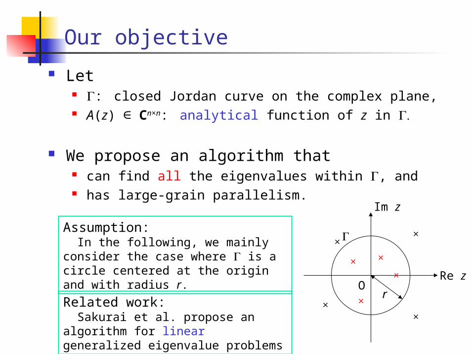
Let : closed Jordan curve on the complex plane, A(z) ∈ Cn×n: analytical function of z in

We propose an algorithm that can find all the eigenvalues within , and has large-grain parallelism.

Im z

Re zO

Assumption: In the following, we mainly consider the case where is a circle centered at the origin and with radius r.

Related work: Sakurai et al. propose an algorithm for linear generalized eigenvalue problems

r

Our approach

The basic idea Let f(z) = det(A(z)). Then f(z) is an analytical function of z in and the

eigenvalues of A(z) are characterized as the zeros of f(z).

Use Kravanja’s method (Kravanja et al., 1999) to find the zeros of an analytic function.

Finding zeros of f(z)

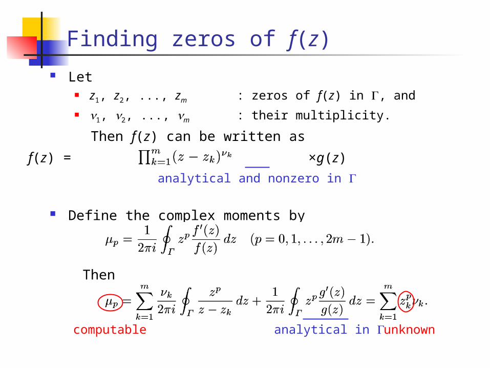
Let z1, z2, ..., zm : zeros of f(z) in , and 1, 2, ..., m : their multiplicity.

Then f(z) can be written as

Define the complex moments by

Then

f(z) = ×g(z)

analytical and nonzero in

analytical in unknowncomputable

Finding zeros of f(z) (cont'd)

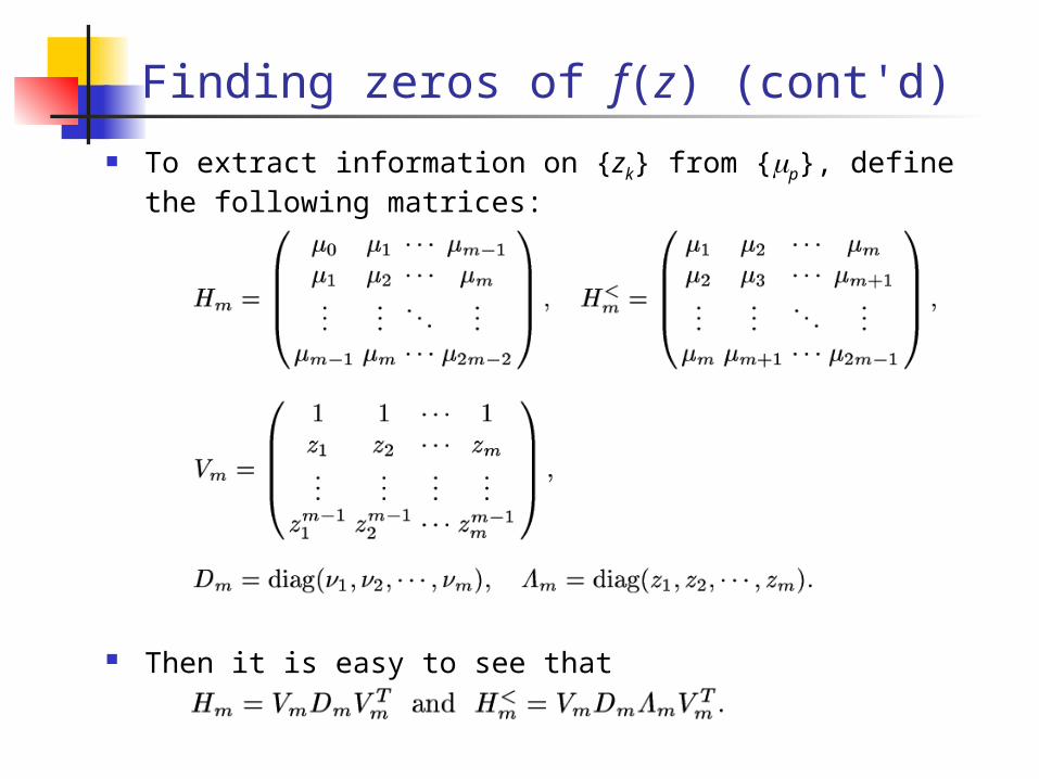
To extract information on {zk} from {p}, define the following matrices:

Then it is easy to see that

Finding zeros of f(z) (cont'd)

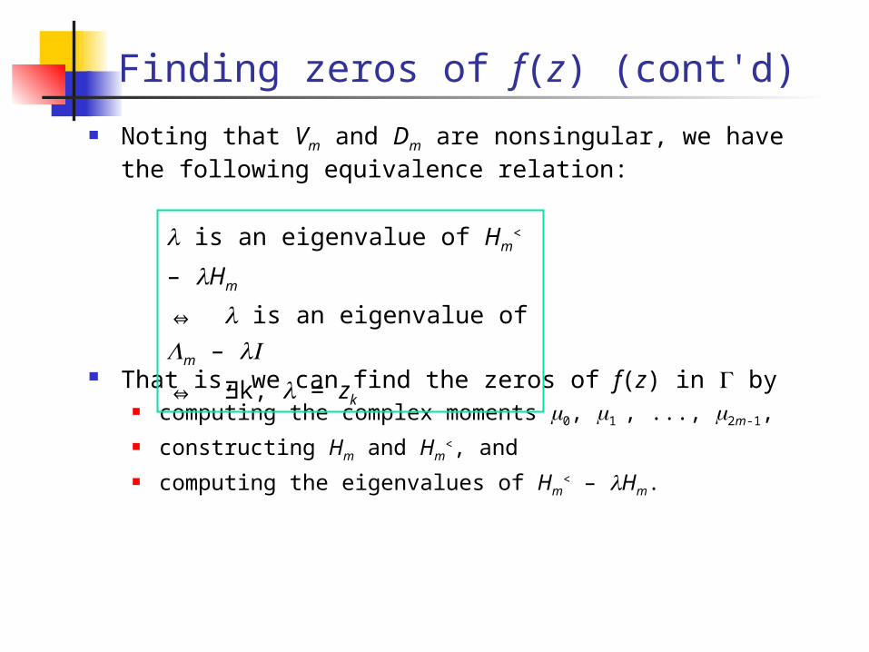
Noting that Vm and Dm are nonsingular, we have the following equivalence relation:

That is, we can find the zeros of f(z) in by computing the complex moments 0, 1 , ..., 2m-1, constructing Hm and Hm

<, and computing the eigenvalues of Hm

< – Hm.

is an eigenvalue of Hm< – Hm

⇔ is an eigenvalue of m –

⇔ ∃k, = zk

Application to the nonlinear eigenvalue problem

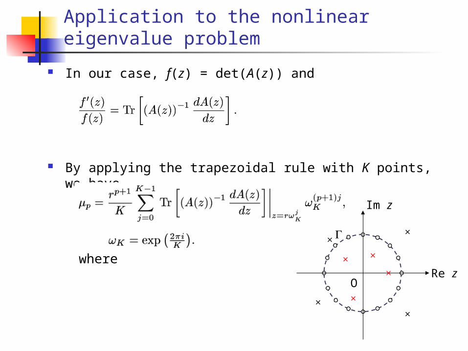
In our case, f(z) = det(A(z)) and

By applying the trapezoidal rule with K points, we have

where

Im z

Re zO

The algorithm

The computationally intensive part.Large-grain parallelism

Detecting and removing spurious eigenvalues

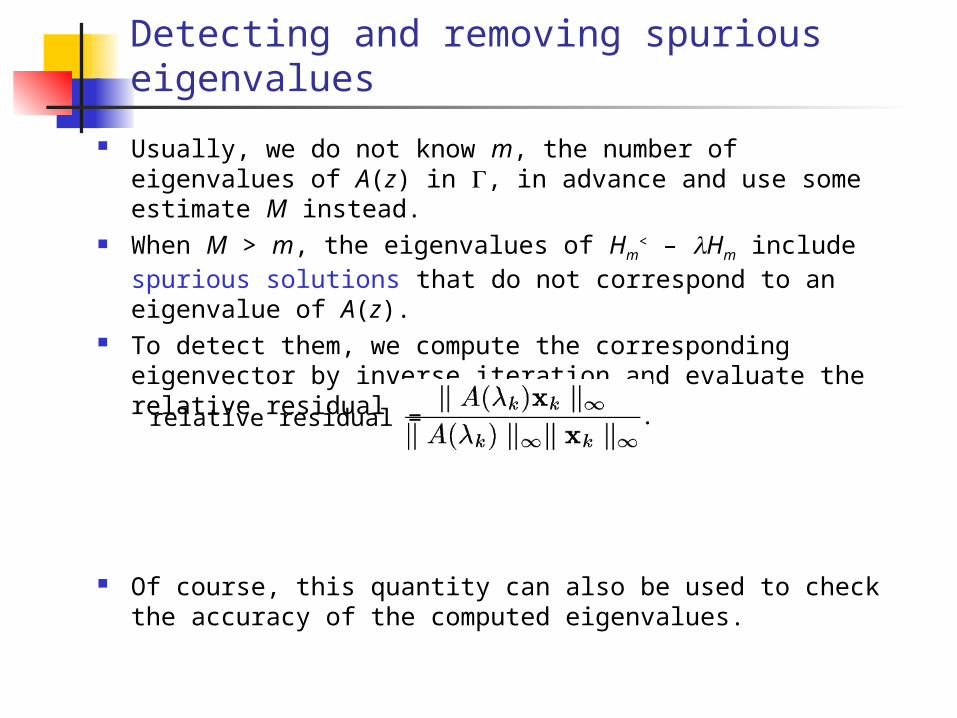
Usually, we do not know m, the number of eigenvalues of A(z) in , in advance and use some estimate M instead.

When M > m, the eigenvalues of Hm< – Hm include spurious

solutions that do not correspond to an eigenvalue of A(z). To detect them, we compute the corresponding

eigenvector by inverse iteration and evaluate the relative residual defined by

Of course, this quantity can also be used to check the accuracy of the computed eigenvalues.

relative residual =

Numerical results

Test problem A(z) = A – zI + B(z), where

A(z) : real random nonsymmetric matrix B(z) : antidiagonal matrix with antidiagonal elements ez

: parameter to specify the strength of nonlinearity Parameters

n = 500, 1000, 2000 0, 10–4, 10–3, 10–2, 10–1

Computational environment Fujitsu HPC2500 (SPARC 64IV), 1-16 processors Program written with C and MPI LAPACK routines were used to compute (A(z))–1 and to

compute the eigenvalues of Hm< – Hm.

Accuracy of the computed eigenvalues

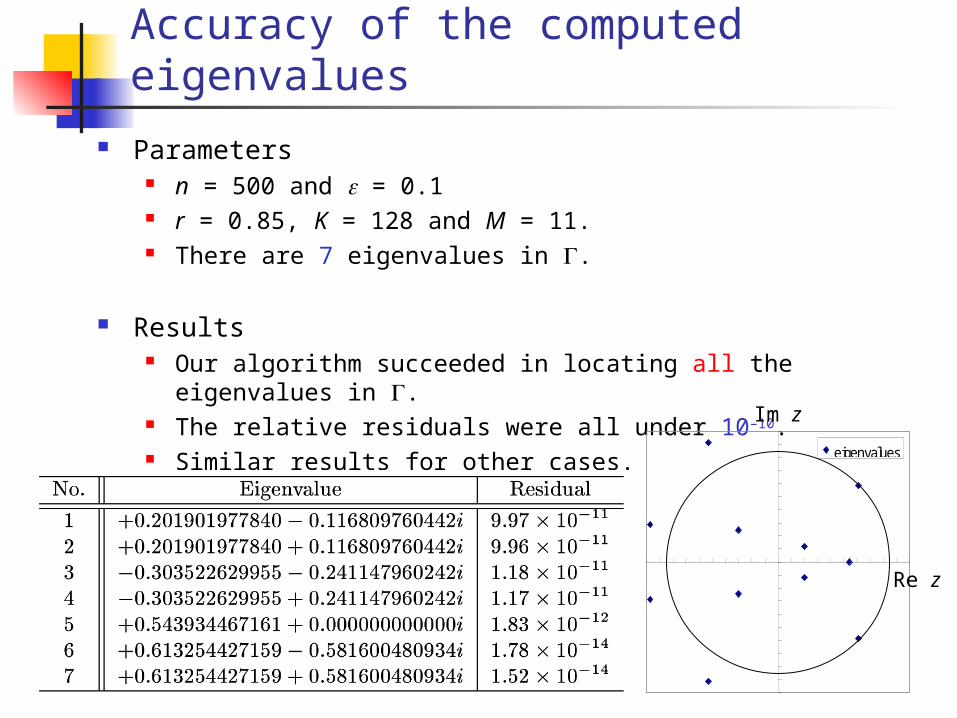
Parameters n = 500 and = 0.1 r = 0.85, K = 128 and M = 11. There are 7 eigenvalues in .

Results Our algorithm succeeded in locating all the eigenvalues in

. The relative residuals were all under 10–10. Similar results for other cases.

eigenvalues

Im z

Re z

Effect of K and M on the accuracy

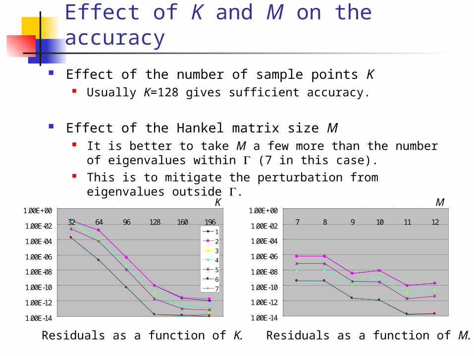
Effect of the number of sample points K Usually K=128 gives sufficient accuracy.

Effect of the Hankel matrix size M It is better to take M a few more than the number of

eigenvalues within (7 in this case). This is to mitigate the perturbation from eigenvalues

outside .

1.00E-14

1.00E-12

1.00E-10

1.00E-08

1.00E-06

1.00E-04

1.00E-02

1.00E+00

32 64 96 128 160 1961

2

3

4

5

6

7

1.00E-14

1.00E-12

1.00E-10

1.00E-08

1.00E-06

1.00E-04

1.00E-02

1.00E+00

7 8 9 10 11 12

Residuals as a function of K. Residuals as a function of M.

K M

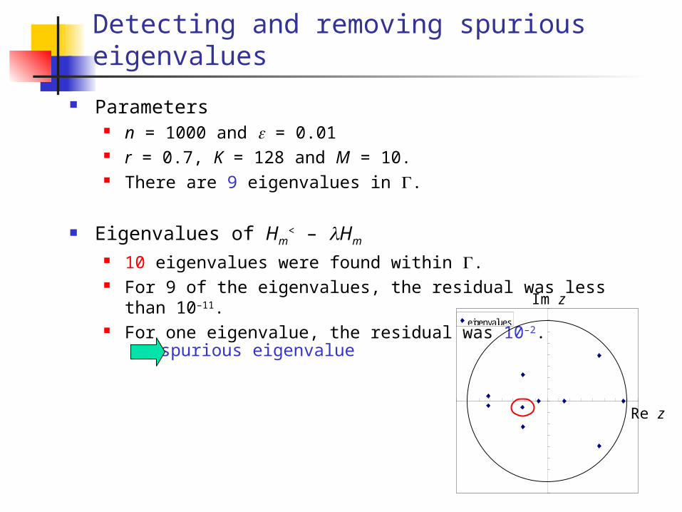
Detecting and removing spurious eigenvalues

Parameters n = 1000 and = 0.01 r = 0.7, K = 128 and M = 10. There are 9 eigenvalues in .

Eigenvalues of Hm< – Hm

10 eigenvalues were found within . For 9 of the eigenvalues, the residual was less than 10–11. For one eigenvalue, the residual was 10–2.

eigenvalues

Im z

Re z

spurious eigenvalue

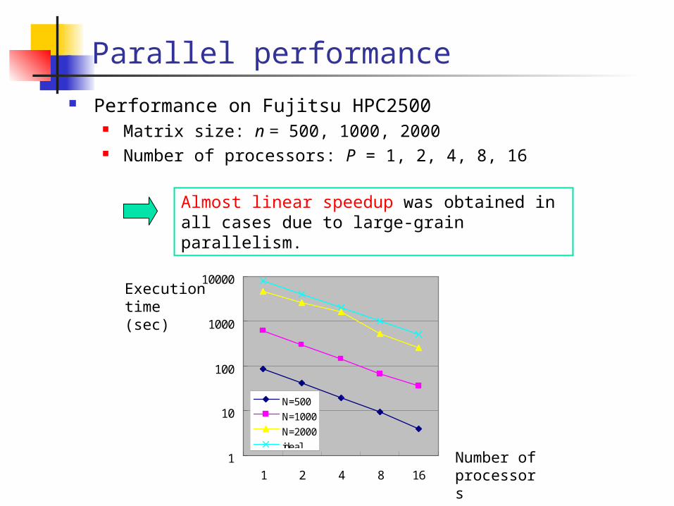
Parallel performance

Performance on Fujitsu HPC2500 Matrix size: n = 500, 1000, 2000 Number of processors: P = 1, 2, 4, 8, 16

1

10

100

1000

10000

1 2 4 8 16

N=500N=1000N=2000ideal

Execution time (sec)

Number of processors

Almost linear speedup was obtained in all cases due to large-grain parallelism.

Parallel performance (cont'd)

Performance in a Grid environment Matrix size: n = 1000 Machine: Intel Xeon Cluster Master-worker type parallelization using OmniRPC

(GridRPC)

Execution time

Number of processors

Good scalability was obtained for up to 14 processors.

0:00:00

0:30:00

1:00:00

1:30:00

2:00:00

2 4 6 8 10 12 140

2

4

6

8

10

12

14

16Speedup

Summary of this study

We proposed a new algorithm for the nonlinear eigenvalue problem based on complex contour integration.

Our algorithm can find all the eigenvalues within a closed curve on the complex plane. Moreover, it has large-grain parallelism and is expected to show excellent parallel performance.

These advantages have been confirmed by numerical experiments.

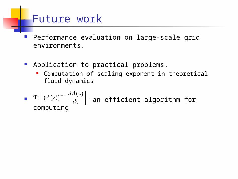
Future work

Performance evaluation on large-scale grid environments.

Application to practical problems. Computation of scaling exponent in theoretical fluid

dynamics

Development of an efficient algorithm for computing