1

A. La Rosa Lecture Notes

INTRODUCTION TO QUANTUM MECHANICS PART-III THE HAMILTONIAN EQUATIONS and the

SCHRODINGER EQUATION ________________________________________________________________

CHAPTER-8 FROM THE HAMILTONIAN EQUATIONS TO THE SCHRODINGER EQUATION. The case of an electron propagating in a crystal lattice

8.1 Hamiltonian for an electron propagating in a crystal lattice

8.1.A Defining the Base States and the Hamiltonian Matrix

8.1.B Stationary States Energy bands

8.1.C Time-dependent States

Electron wave-packet and group velocity

Effective mass (case of low energy electrons)

8.2 Hamiltonian equations in the limit when the lattice space tends to zero

8.2.A From a discrete to a continuum basis

8.2.B The dependence of amplitude probability on position.

Transition from describing a quantum state I in very general terms, to a detailed account of the amplitude-probability dependence on

position x

8.2.C Equation describing an electron in an external potential

V = V( x, t )

8.3 The Postulated Schrodinger Equation

References:

Feynman lectures Vol. III, Chapters 13 and 16.

2

CHAPTER-8 FROM THE HAMILTONIAN EQUATIONS TO THE SCHRODINGER EQUATION.

One of the purposes of this chapter is to show that the correct fundamental quantum mechanics equation (the Schrödinger equation) has the same form that one obtains for the limiting case when 0b of an electron moving along a line of atoms separated by a distance b from each other. Starting from a problem where an electron moves along a set of discretely separated atoms along a line, an equation is obtained for the case in which the separation distance tends to zero. This procedure can help us understand better the interpretation of the wavefunction solutions of the Schrödinger equation.

8.1 Hamiltonian for an electron propagating in a crystal lattice1

In our study of a two-state system, we learned that there is an amplitude probability for the system to jump back and forth to the other energy state.

Similarly in a crystal,

One can imagine an electron in a „well‟ at one particular atom and with some particular energy.

Suppose there is an amplitude probability that the electron move into another „well‟‟ at one of the nearby atom.

From its new position it can further move to another atom or return to its initial „well‟.

xn

b

x1

This study will allow understanding an ubiquitous phenomenon in nature that if the lattice were perfect (i.e. nodefects), the electrons would able to travel through the crystal smoothly and easily, almost as if they were in vacuum.

3

8.1.A Defining the base states and the Hamiltonian matrix

We would like to analyze quantum mechanically the dynamics of an extra electron put in a lattice (as if to produce one slightly bound negative ion).

Some considerations first:

a) An atom has many electrons. However many of them are quite bounded that to affect their state of motion a lot of energy (in excess of 10 eV) is needed. We will assume that the motion of an extra electron (weakly bounded to the atom, the depth of the „well‟ is much smaller than 10 eV.) It is the dynamics of this weekly bounded electron that we are interest in.

b) What would be a reasonable set of base states?

We could try the following:

1 crystal state in which the e- is in the atom 1.

2 crystal state in which the e- is in the atom 2.

…

n crystal state in which the e- is in the atom n.

…

(1)

Any state t of the one-dimensional crystal can then be

expressed as,

( t ) = n

n An( t ) = n

n n ( t ) (2)

where the scalars An( t ) = n ( t ) are the amplitude probabilities

of finding the state ( t ) in the base states n, respectively,

at the time t.

The evolution of An( t ) as a function of time is determined by

)()()(

tAtHdt

tdAi jjn

n

j (3)

So we need to find the coefficients Hnj first.

c) How is the Hamiltonian going to look like? That is, how to find the

coefficients Hnj ?

4

We proceed similarly to the case of the ammonia molecule (treated in the previous chapter.) Since all the atoms sites in the crystal are energetically equivalent, we can assume

Hnn = Eo , n = 1,2, 3, … (4)

On the other hand, an electron can move from one atom to any other atom, thus transferring the negative ion to another place. We will assume however that the electron will jump only from one atom to the neighbor of either side. That is, for a given n,

Hn (n+1) ≡ -W , Hn (n-1) ≡ -W. (5)

and

Hnj =0 for j ≠ n ± 1.

The equation of motion (3) takes the form

…

dt

dAi n-1 -W An-2 + Eo An-1 - W An

dt

dAi n - W An-1 + Eo An - W An+1 (6)

dt

dAi n 1 -W An + Eo An+1 -W An+2

…

8.1.B Stationary States

From our experience studying the ammonia molecule, let‟s recall

that after identifying two “localized” sates 1 and 2 , we were able

to find two peculiar stationary states SI and SII,

SI ≡2

1( 1 + 2 ) and SII ≡

2

1( 1 - 2 )

which had the following dependence on time (see Chapter 7, expression (51)),

SI( t ) =t

1Ei/e )(

SI ( 0 ) , where EI = E0 - W

5

SII( t ) =t

IIEi/e )(

SII (0) where EII = E0 + W

That is, SI and SII, are states of definite energy.

We want to highlight the peculiar phase with which the states 1 and

2 participate in SI and SII.

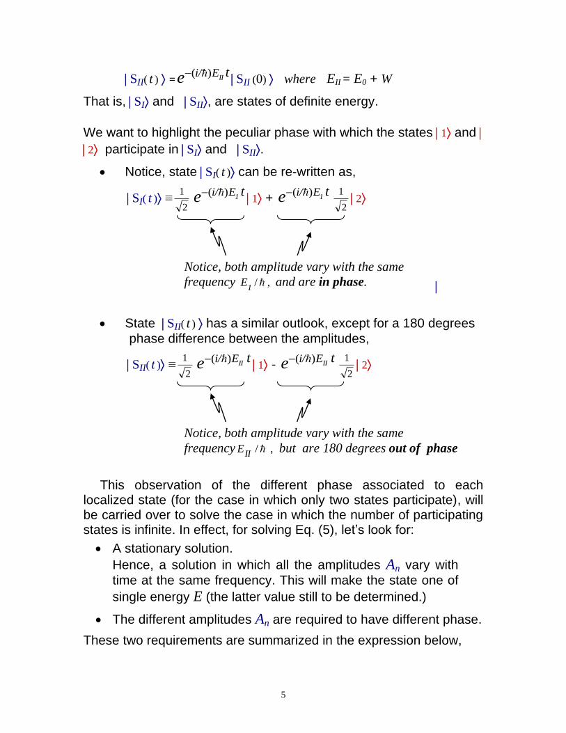
Notice, state SI( t ) can be re-written as,

SI( t ) ≡2

1 t 1

Ei/e )( 1 +

t 1

Ei/e )(

2

1 2

Notice, both amplitude vary with the same

frequency /1

E , and are in phase.

State SII( t ) has a similar outlook, except for a 180 degrees

phase difference between the amplitudes,

SII( t ) ≡2

1 t II

Ei/e )( 1 -

t II

Ei/e )(

2

1 2

Notice, both amplitude vary with the same

frequency /II

E , but are 180 degrees out of phase

This observation of the different phase associated to each localized state (for the case in which only two states participate), will be carried over to solve the case in which the number of participating states is infinite. In effect, for solving Eq. (5), let‟s look for:

A stationary solution.

Hence, a solution in which all the amplitudes An vary with

time at the same frequency. This will make the state one of

single energy E (the latter value still to be determined.)

The different amplitudes An are required to have different phase.

These two requirements are summarized in the expression below,

6

An( t ) = an

t Ei/e ))(( (7)

We are therefore looking for a stationary solution of the form,

( t ) = n

n An

( t ) = n

n ant Ei/e ))((

(7)‟

All the amplitude-probabilities oscillate

at the same frequency )( E/ , but with

potentially different phase between each

other; that is, the different an are

complex numbers.

We have to find values for E and the different an compatible with Eq.

(5).

Replacing (7) in (5)

Ean = - W an-1 + Eo an - W an+1 (8)

If we label the atoms by their positions,

xn = n b

where b is the spacing between contiguous atoms in the crystal

equation (8) takes the form,

Ea(xn) = - W a(x n-1) + Eo a(xn) - W a(x n+1) (9)

Trial solution,

a( xn) = nkie x

(the value of k to be determined) (10)

Replacing (10) in (9) one obtains,

E nkie x

= - W 1x

n-ki

e + Eo nkie x

- W 1x

nki

e

E = - W b kie + Eo - W b kie

E = Eo - W [ b kie + b kie ]

7

E(k) = Eo - 2W Cos (k b) (11)

We realize, for any real value of k there is an energy E(k)=Eo-

2WCos(k b) and an infinite-set of values a(xn) = nkie x

, which, when

replaced in (7)‟ constitute a stationary solution of Eq. (6). It would appear that there are an infinite number of solutions (one for each

real value of k that can occur to us.) We will see later that this is not

completely true.

Summary. We have found that for any given real value of k,

There exists a corresponding stationary solution

k( t ) =n

n Ank

( t ) = n

n nkie x t kEi/e ])[( )(

of energy

E(k) = Eo - 2W Cos( k b))

Notice the amplitude probabilities vary with time as,

Ank

( t ) = nkie x

t E(k)i/e ][ )(

The expression above indicates the electron is equally likely to

be found at every atom, since all the quantities Ank( t )

2 are

equal (independent of n). Only the phase is different for

different atom location, changing in the amount ( k b) from atom

to atom.

xn

b

Real Ank

Fig 8.1 Real part of the amplitude probability An for finding the

atom location of the extra electron in the crystal, at a given time.

8

The energy E as a function of k is shown in the figure below.

Only energies in the range from E -2W to E +2W are allowed. If an electron in a crystal is in a stationary state, it can have no energy other than values in this band.

(This allows understanding the energy bands formation in a crystal, which explains the working principle of electrical conductivity in metals and semiconductors.)

The smallest energies E ~ (Eo -2W) are obtained for the

smallest values of k 0. As k increases, the energy

increases as well until it reaches a maximum at k =/ b

For k larger than / b the energy would start to decrease, but

there is no need to consider such values, because they do not give new states.

Eo+2W

-/ b

Eo-2W

/ b

E

k

Eo

No need to consider these

values of k.

No need to consider these

values of k.

Fig 8.2 Energy of the stationary states as a function of k, where k is

the wave-vector of the state k=n

nAnk=

n

n nkie x t)kE(i/ e ])[(

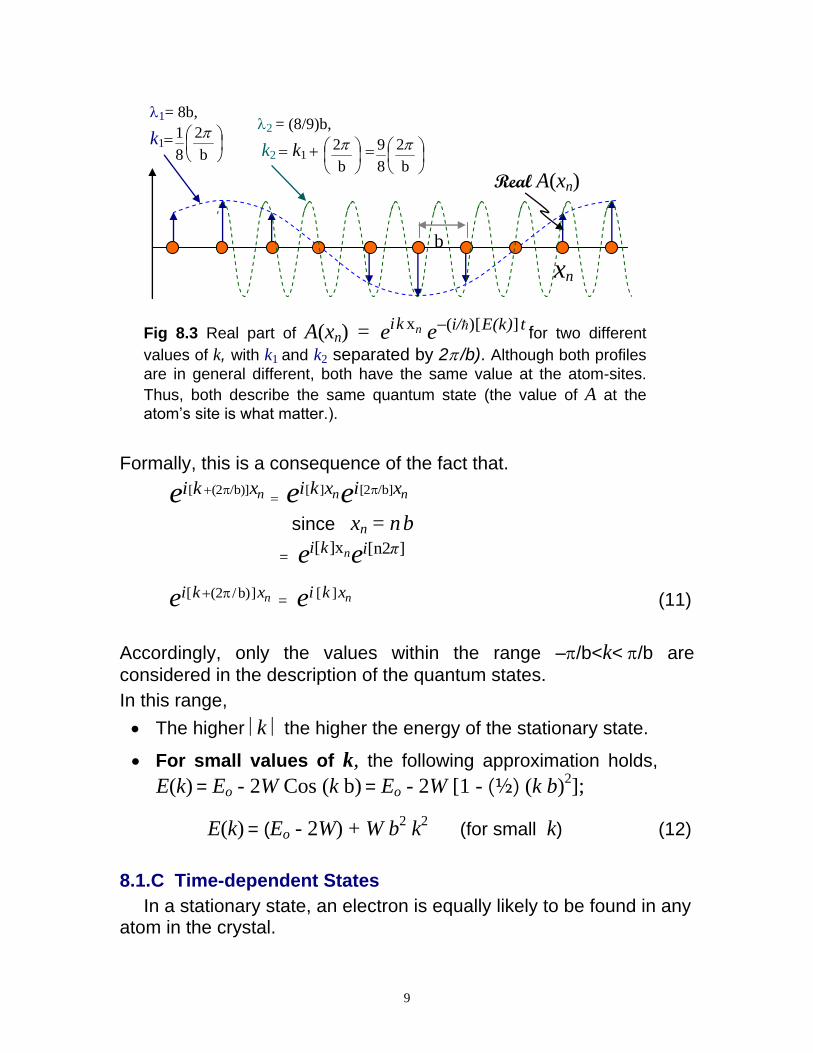
In effect, while a wave-vector k2 = k1+2/b has a profile of higher spatial and thus is indeed different than that the profile corresponding

to the wave-vector k1, it turns out that both profiles have the same value at each atom location (see Fig. 8.3 below). Hence, as far as the evaluation of the probability-amplitude at the atoms-site is concerned, both wave-vectors describe the same quantum state.

9

xn

b

Real A(xn)

1= 8b,

k1

b

2

8

1 2 = (8/9)b,

k2 k1

b

2

b

2

8

9

Fig 8.3 Real part of A(xn) = nkie x t E(k)i/e ])[( for two different

values of k, with k1 and k2 separated by 2/b). Although both profiles

are in general different, both have the same value at the atom-sites.

Thus, both describe the same quantum state (the value of A at the

atom‟s site is what matter.).

Formally, this is a consequence of the fact that.

nxkie /b)](2[

nn xixki ee /b][2][

since xn = n b

= ][n2x][ πiki ee n

nxkie ]b)/(2[ = nxkie ][

(11)

Accordingly, only the values within the range –/b<k</b are

considered in the description of the quantum states.

In this range,

The higher k the higher the energy of the stationary state.

For small values of k, the following approximation holds,

E(k) = Eo - 2W Cos (k b) = Eo - 2W [1 - (½) (k b)2];

E(k) = (Eo - 2W) + W b2 k

2 (for small k) (12)

8.1.C Time-dependent States

In a stationary state, an electron is equally likely to be found in any atom in the crystal.

10

In contrast, how to represent a situation in which an electron of a certain energy is located in a certain region? That is, a situation in which an electron is more likely to be found in one region than at some other place?

Electron wave-packet

An alternative is to make a wave-packet, out of a proper linear

combination of the stationary states k( t ) found in the previous section,

k( t ) =n

n Ank

( t ) = n

n nkie x t kEi/e ])[( )( . (Each stationary

state identified by the value of k.)

For example, we can make a wavepacket that peaks around a

given atom at xno. That is, in the expansion

( t ) =n

xn An( t ) =n

xn A (xn, t )

the amplitude A (xn, t ) peaks around the no-th atom (at a given time

t.)

xn

b

Real A(xn, t)

Fig. 8.4 Profile (dashed blue line) of the real part of the wavepacket

at a given time t.

For a localized (in space) pulse A(xn, t), there will be an associated

Fourier transform F(k) with a predominant wavenumber ko and all

the other wavenumbers k within a range k: that is,

dkt/-xki

FA

k

E(k)k

πtx nen

}{ ][

)(2

1) ,(

Using

)()(

kEk ,

11

dkt-xki

FA

k

kk

πtx nen

}{ )(

)(2

1) ,(

Group velocity

We learned in Chapter-4 that, even though the k-components travel at different phase velocities, still we can define a velocity for the wave-packet called the group velocity,

oocitygroup-vellon'swavefuncti

kokg

k

kd

k

k

dd

d )) 1 vv

If ko is in the low-energy range, then we can use expression (12)

for the energy, which gives

ok

W

2

gocitygroup-vellon'swavefuncti

b2vv (for small values of k ) (13)

Velocity of a low-energy wave-packet

having a predominant wavenumber k=ko,

Effective mass (case of low energy electrons)

Since E(k) = (Eo - 2W) + W b2 k

2 (for small values of k,) we realize that low-energy electrons move with energy proportional to the square of its velocity, like a classical particle. Indeed, this resemblance with a classical particle can be made more transparent through the definition of an effective mass. For that purpose, first let‟s move our zero

energy reference to (Eo -2W), as to obtain,

E = W b2k2 .

12

-/ b / b k

4W

0

E

2W

States of

low energy

( k<</b ) Fig. 8.5 Relative to Fig. 8.2 the minimum energy has been moved to the zero energy level. Accordingly, E(k) = 2W - 2W

Cos( k b).

A wave-packet of predominant wave-vector k=ko will have an energy

equal to E= W b2ko2 . I terms of the associated group velocity, given in

(13) above), the energy can be expressed as

E = W b2

2

2)(

2

v

bW

g=

2

g

2

2)v(

b4

1

W.

Thus, for a wavepacket whose predominant wave-vector k is

relatively small compared to /b, one obtains,

2

gv

2b2

2

2

1E

W

(14)

This expression can be written as

2

geffvm

2

1E (15)

13

for, thus, resembling the motion of the quantum packet with the classical description of the motion of an electron. That is, amplitude-probability waves behave like a particle.

The constant effm is called the “effective mass”.

2

2

2 bWmeff

(for small values of k ) (16)

effm has nothing to do with the electron‟s mass. It has been

defined as to resemble the motion of a classical particle. In a real crystal it turns out to have a magnitude of about 2 to 20 times the free-space mass of an electron.

Notice however the appealing to interpret meff as a real mass:

For example, the smaller W the greater the meff; that is, a

smaller amplitude probability (W) for an electron to move from one position to another is translated into an equivalent heavier mass inertia.

Notice also, from (13) and (16),

ogeff km v (17)

where ko is the predominant wavenumber of the wavepacket

We understand now how an electron can ride through the crystal,

flowing perfectly free (with v = vgroup) despite having all the atom to

hit against. It does by having its amplitude probability flying from one atom to the next, with W providing the quantum probability to move from one atom to the next. That is how a solid conduct electricity.

8.2 Hamiltonian equations in the limit when the lattice space tends to zero

In the previous section we realized that “an amplitude-probability (wavepacket)” propagate in a crystal as if it were a particle. For example, its was found that its energy is

equal to ½ meffvg2, its de Broglie momentum o

k is equal to meffvg.

That is, the Hamiltonian description of amplitude-probability waves

14

in a lattice-crystal resembles the mechanistic description of a particle.

One would expect then that the Hamiltonian description of amplitude probability waves in a discrete lattice would inherently have in it (or be nothing but a mirror reflection of) a more general quantum mechanical description of a particle. Maybe by taking the limiting case of the lattice distance “b” equal to zero, the resulting continuum equation would resemble the more formal Schrodinger equation. The latter is precisely the objective to be pursued in this section.

Incidentally, this chapter offers also an opportunity to illustrate the academic transition from a) the until now somewhat loose and very

general description of a quantum state I, to b) a much more detailed description, i.e. giving an account on how the amplitude-

probability‟s (x) depends on the position coordinates.

8.2.A From a discrete basis to a continuum basis

Let‟s first formalize the definition of a continuum spatial basis

Let‟s take a linear lattice, and imagine that the lattice spacing “b” were to be taken smaller and smaller. In the limit, we would have the case in which the electron could be anywhere along the line.

In other words, assume the possibility of labeling the space with infinity of points (in a continuous fashion.)

Discrete case Continuum case

xn 0b

x (18)

x stands for a state in which a particle is located at a spatial coordinate x.

= n

xn [ A (xn) ]

will be also written as

= n

xn [ A (xn) ]

We use A instead of simply A,

as to make more explicit that the

15

amplitude probabilities corres-

ponds to the state .

We know that xn =[A (xn)] (Notice the expression on the left

constitutes a better notation,

emphasizing that there is no need

to include the character A.)

xn gives the amplitude

probability of the general

state to be found at xn.

Alternatively the following notation is also used,

xn = [A (xn)]≡ (xn) 0b

x = A (x) ≡(x).

amplitude probability

to find the state at

the state x . (19)

Note: Pay attention to the potential confusion that may occur

when writing x ≡ (x ). The same symbol is being used for,

i) labeling a particular physical state of an electron; and ii)

defining a mathematical function of x(x), which gives the

amplitude probability that an electron in the state be found at

the state x .

8.2.B From a general reference of the states I, to a detailed account of the amplitude-probability on the spatial

position x, xIf we can work out the equations that relate the value of the

amplitude-probability at one point x to the amplitude-probability at

neighboring points, then we would have the quantum mechanical description of an electron‟s motion in the continuum space.

Discrete case. Let‟s start review the results we have for the discrete case. For a lattice the Hamiltonian equations are,

16

dt

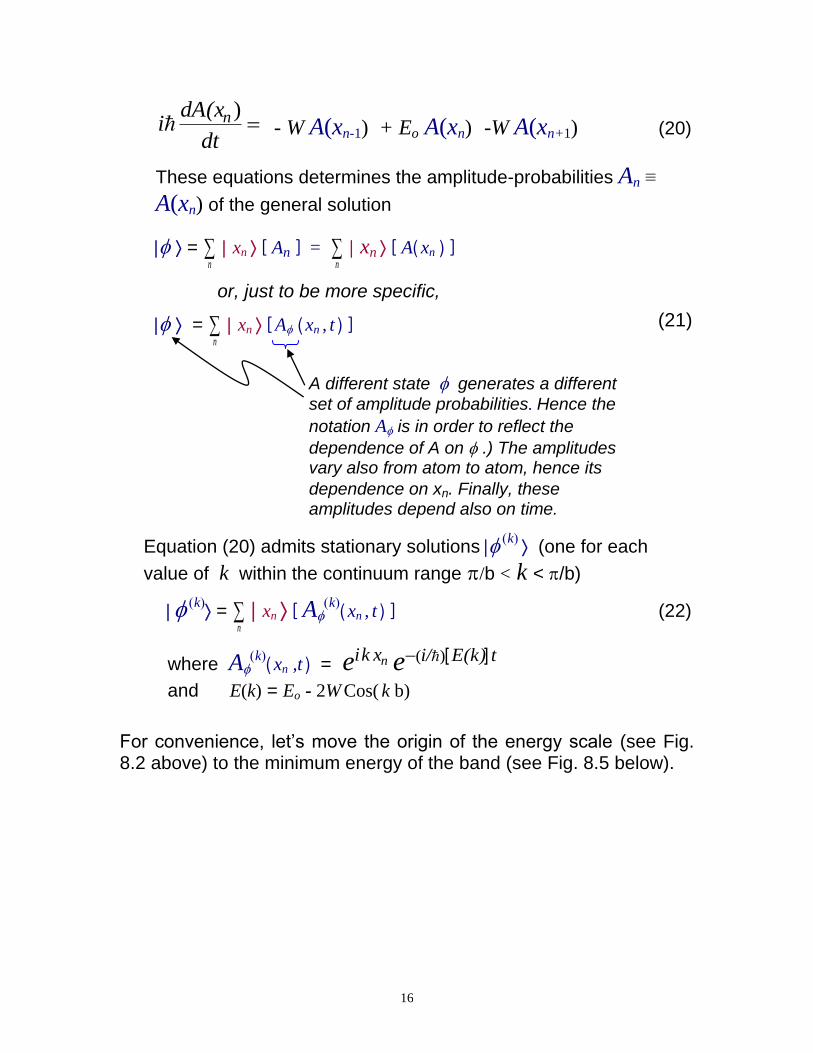
dA(xi n ) - W A(xn-1) + Eo A(xn) -W A(xn+1) (20)

These equations determines the amplitude-probabilities An ≡

A(xn) of the general solution

= n

xn [ An ] = n

xn [ A( xn ) ]

or, just to be more specific,

= n

xn [ A ( xn , t ) ]

A different state generates a different

set of amplitude probabilities. Hence the

notation A is in order to reflect the

dependence of A on .) The amplitudes vary also from atom to atom, hence its

dependence on xn. Finally, these amplitudes depend also on time.

(21)

Equation (20) admits stationary solutions k (one for each

value of k within the continuum range /b < k < /b)

k =

n

xn [ Ak

( xn , t ) ] (22)

where Ak

( xn ,t ) = nxkie

t E(k)i/e ][ )(

and E(k) = Eo - 2W Cos( k b)

For convenience, let‟s move the origin of the energy scale (see Fig. 8.2 above) to the minimum energy of the band (see Fig. 8.5 below).

17

4W

-/ b

0

/ b

E

k

2W

Fig. 8.5 Relative to Fig. 8.2 the minimum energy has been moved to the zero energy level. Accordingly, Eo= 2W and E(k) =

2W - 2W Cos( k b). (Here Eo=Hnn is the energy of the electron

when located in an isolated atom.)

Let’s analyze now the continuum case, by taking the limit 0 b .

We start from the discrete case, Eq. (20), which governs the behavior

of the amplitude probabilities A ( xn , t ) These components make up the state

= n

xn [ A ( xn , t ) ]

In the new energy scale, indicated in Fig. 8.5), the equations in (20) become

dt

dA(xi n ) - W A(xn-1) + 2W A(xn) - W A(xn+1) (23)

Rearranging terms,

dt

dA(xi n ) W [A(xn) - A(xn-1)] - W [A(xn+1) - A(xn)]

W b1-nn

1-nn

x x

A(xA(x

)) - W b

nn

n1n

x x

A(xA(x

1

))

(Notice above that for simplicity we are using A( xn ) but we should be

using A( xn , t ), as the A‟s define the state )

Now we take 0 b

18

dt

dA(xi n ) W b )n(x

dx

dA - W b )

1n(x

dx

dA

= - W b [ )1n

(xdx

dA - )n(x

dx

dA ]

= - W b2 )

1n(x

dx

Ad2

2

dt

xdAi n )( - W b

2 )b( nx

dx

Ad2

2

(24)

If we blindly took 0b , expression (24) would give 0)( nxdt

dAi ,

which would reveal no useful information. Recall however that W

gives the likelihood the electron jumps to the neighbor atom and, thus, it is plausibly to think that as the spacing “b” decreases the

value of W simultaneously increases. Thus, we could conveniently

consider that as “b” decreases, the product W b2 remains constant.

Similar to expression (16) we can call this factor effm

bW2

22 .

So we will consider that as b 0, the value of W increases such that

the product W b2

remains constant and equal to )2/(eff

2m .

effmbbW

20

22

Consequently, as 0b , Eq. 24 becomes,

dt

tx,dAi

)(

effm2

2 2

2

dx

t)A(x,d (25)

19

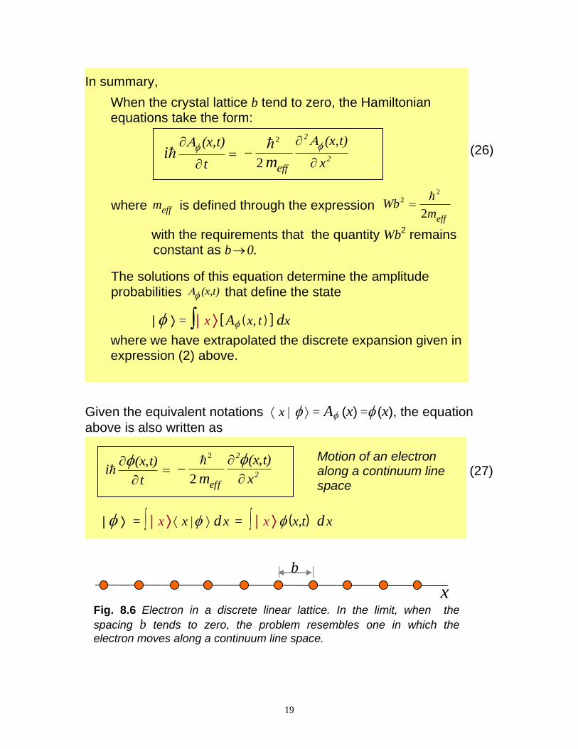
In summary,

When the crystal lattice b tend to zero, the Hamiltonian equations take the form:

t

t)(x,i

2

2

x

t)(x,

ffem

2

2

.

where effm is defined through the expression effm

bW2

22

with the requirements that the quantity Wb2 remains

constant as b0.

The solutions of this equation determine the amplitude probabilities t)(x, that define the state

= x [ A( x, t ) ] dx

where we have extrapolated the discrete expansion given in expression (2) above.

(26)

Given the equivalent notations x = A (x) =(x), the equation

above is also written as

t

t)(x,i

2

2

x

t)(x,

effm

2

2

.

= x x d x = x (x,t) d x

Motion of an electron along a continuum line space

(27)

x

b

Fig. 8.6 Electron in a discrete linear lattice. In the limit, when the

spacing b tends to zero, the problem resembles one in which the

electron moves along a continuum line space.

20

8.2.C Particle in a potential V=V( x,t )

What would be the limiting case 0b of the Hamiltonian equations if the atoms were subjected to an external potential?

For comparison, let‟s take a look to the Hamiltonian equations

corresponding to the case V(x)=0, which was given in the expression (6) and reproduced below,

…

dt

dAi n-1 W An-2 + Eo An-1 W An

dt

dAi n W An-1 + Eo An W An+1 (28)

dt

dAi n 1 W An + Eo An+1 W An+2

…

First, let‟s recall that Eo is the energy of the electron when located

in an isolated atom.) When no external voltage is applied, all the

atoms are equivalent; accordingly Eo =Hnn ( n=1, 2,3,…)

However when an external voltage is applied, the electron potential energy varies from atom to atom (for example if an uniform

electric field E were applied, then a potential Vn= - Exn would be

established.) Thus, in the case of a general voltage V = V(x) were

applied, the energy Eo of an electron will be shifted to Eo+Vn where

Vn ≡V( xn )

dt

dAi n -W An-1 + ( Eo+Vn )An - W An+1 (29)

This is practically the same Eq. (20); only the elements along the diagonal become modified. The application of taking the limiting process 0b becomes, then, very similar. We should obtain,

t

t)(x,Ai

t)(x,At,x

x

t)(x,A

mV

2

2

eff

)(

2

2

Or, equivalently

21

t

tx,i

)( )()(

)(

2

2

tx,tx,Vx

tx,

m 2

2

eff

(30)

= x x dx = x (x,t) dx

8.3 The Postulated Schrodinger Equation

Non-relativistic particle motion

The correct quantum mechanical equation for the motion of an electron in free space was first discovered by Schrodinger.

t

t)(x,i

2

2

x

t)(x,

m 2

2

(31)

Schrodinger equation

(free particle)

Notice that the Schrodinger equation is very similar to the equation (26) above.

“We do not intend to have you think we have derived the Schrodinger equation but only wish to show you one way of thinking about it. When Schrodinger first wrote it down, he gave a kind of derivation based on some heuristic arguments and some brilliant intuitive guesses. Some of the arguments he used were even false, but that does not matter; the only important thing is that the ultimate equation gives a correct description of nature.”

“The purpose of the discussion in the previous section was to show that:

the correct fundamental quantum mechanics equation (31),

has the same form than,

the equation (27 ) obtained when considering the limiting case of an electron moving along a line of atoms.”

“This means that we can think of Eq. (31) as describing the diffusion

of a probability amplitude (x,t) from one point to the next along the line.”

“That is, if an electron has a certain amplitude probability to be at one point, it will, a little time later, have some amplitude to be at neighboring points.”

22

Taken from “The Feynman Lecture on Physics, Vol III, page 16-4.

The diffusion argument given above springs from the fact that the Schrodinger equation (31) looks very similar to the diffusion equation

t

2

2

x

D , (the latter governing, for example, the time evolution of a

gas spreading along a tube.)

But, there is a substantial difference between these two equations due to the complex number in front of the time derivative of the

Schrodinger equation

t- i

2

2

xm 2

:

while the diffusion equation leads to exponentially decaying solutions (as tends to a uniform distribution of molecules),

the Schrodinger equation, the imaginary coefficient in front of the time derivative makes the behavior completely different. Its solutions are complex-variable propagating waves.

For a particle moving inside a potential V(x,t) the Schrodinger is,

(32)

),( 2

2

22

txVxmt

i

Schrodinger Equation

“This equation marked a historic moment constituting the birth of the quantum mechanical description of matter. The great historical moment marking the birth of the quantum mechanical description of matter occurred when Schrodinger first wrote down his equation in 1926.

For many years the internal atomic structure of the matter had been a great mystery. No one had been able to understand what held matter together, why there was chemical binding, and especially how it could be that atoms could be stable. (Although Bohr had been able to give a description of the internal motion of an electron in a hydrogen atom which seemed to explain the observed spectrum of light emitted by this atom, the reason that electrons moved this way remained a mystery.)

23

Schrodinger’s discovery of the proper equations of motion for electrons on an atomic scale provided a theory from which atomic phenomena could be calculated quantitatively, accurately and in detail.” Feynman‟s Lectures, Vol III, page 16-13

Although the result (24) is kind of a postulate, we do have some clues about how to interpret it, based on the particular case of the dynamics of an electron in a crystal lattice, studied the sections above.

-----------------------o--------------------------

24

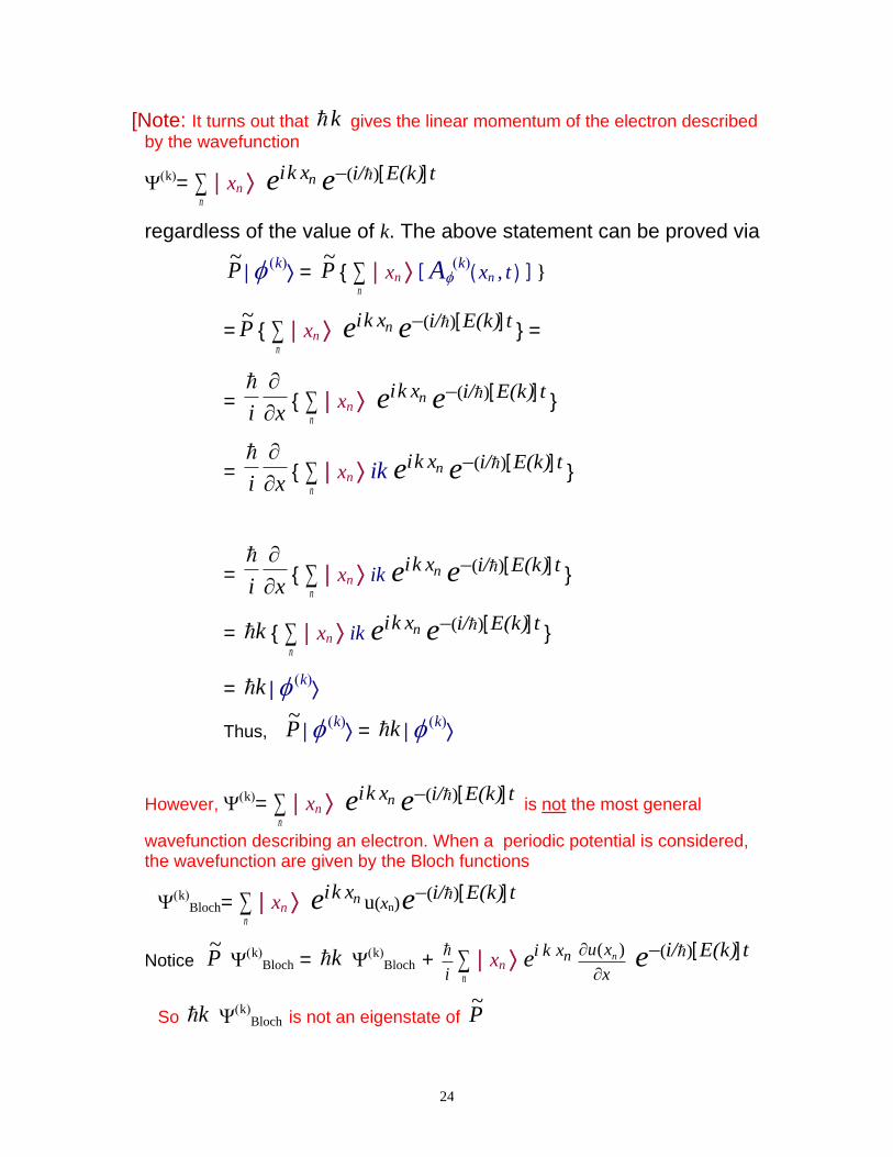
[Note: It turns out that k gives the linear momentum of the electron described

by the wavefunction

k=

n

xn nxkie

t E(k)i/e ][ )(

regardless of the value of k. The above statement can be proved via

P~

k = P

~{

n

xn [ Ak

( xn , t ) ] }

= P~

{ n

xn nxkie

t E(k)i/e ][ )( } =

= xi

{

n

xn nxkie

t E(k)i/e ][ )( }

= xi

{

n

xn ik nxkie

t E(k)i/e ][ )( }

= xi

{

n

xn ik nxkie

t E(k)i/e ][ )( }

= k { n

xn ik nxkie

t E(k)i/e ][ )( }

= k k

Thus, P~

k = k

k

However, k=

n

xn nxkie

t E(k)i/e ][ )( is not the most general

wavefunction describing an electron. When a periodic potential is considered, the wavefunction are given by the Bloch functions

k

Bloch= n

xn nxkie u(xn)

t E(k)i/e ][ )(

Notice P~

kBloch = k

kBloch +

i

n

xn nxkie

x

xu n

)(

t E(k)i/e ][ )(

So k k

Bloch is not an eigenstate of P~

25

But, k is still the crystal momentum of the electron, when this is in the

stationary state k

Bloch

1 The Feynman Lectures, Vol III, Chapter 13