notes on quantum mechanics
DESCRIPTION
Notes on Quantum MechanicsK. SchultenDepartment of Physics and Beckman InstituteUniversity of Illinois at Urbana–Champaign405 N. Mathews Street, Urbana, IL 61801 USA(April 18, 2000)TRANSCRIPT
Notes on Quantum Mechanics
K. Schulten
Department of Physics and Beckman InstituteUniversity of Illinois at Urbana–Champaign
405 N. Mathews Street, Urbana, IL 61801 USA
(April 18, 2000)
Preface i
Preface
The following notes introduce Quantum Mechanics at an advanced level addressing students of Physics,Mathematics, Chemistry and Electrical Engineering. The aim is to put mathematical concepts and tech-niques like the path integral, algebraic techniques, Lie algebras and representation theory at the readersdisposal. For this purpose we attempt to motivate the various physical and mathematical concepts as wellas provide detailed derivations and complete sample calculations. We have made every effort to include inthe derivations all assumptions and all mathematical steps implied, avoiding omission of supposedly ‘trivial’information. Much of the author’s writing effort went into a web of cross references accompanying the mathe-matical derivations such that the intelligent and diligent reader should be able to follow the text with relativeease, in particular, also when mathematically difficult material is presented. In fact, the author’s drivingforce has been his desire to pave the reader’s way into territories unchartered previously in most introduc-tory textbooks, since few practitioners feel obliged to ease access to their field. Also the author embracedenthusiastically the potential of the TEX typesetting language to enhance the presentation of equations asto make the logical pattern behind the mathematics as transparent as possible. Any suggestion to improvethe text in the respects mentioned are most welcome. It is obvious, that even though these notes attemptto serve the reader as much as was possible for the author, the main effort to follow the text and to masterthe material is left to the reader.The notes start out in Section 1 with a brief review of Classical Mechanics in the Lagrange formulation andbuild on this to introduce in Section 2 Quantum Mechanics in the closely related path integral formulation. InSection 3 the Schrodinger equation is derived and used as an alternative description of continuous quantumsystems. Section 4 is devoted to a detailed presentation of the harmonic oscillator, introducing algebraictechniques and comparing their use with more conventional mathematical procedures. In Section 5 weintroduce the presentation theory of the 3-dimensional rotation group and the group SU(2) presenting Liealgebra and Lie group techniques and applying the methods to the theory of angular momentum, of the spinof single particles and of angular momenta and spins of composite systems. In Section 6 we present the theoryof many–boson and many–fermion systems in a formulation exploiting the algebra of the associated creationand annihilation operators. Section 7 provides an introduction to Relativistic Quantum Mechanics whichbuilds on the representation theory of the Lorentz group and its complex relative Sl(2,C). This section makesa strong effort to introduce Lorentz–invariant field equations systematically, rather than relying mainly ona heuristic amalgam of Classical Special Relativity and Quantum Mechanics.The notes are in a stage of continuing development, various sections, e.g., on the semiclassical approximation,on the Hilbert space structure of Quantum Mechanics, on scattering theory, on perturbation theory, onStochastic Quantum Mechanics, and on the group theory of elementary particles will be added as well asthe existing sections expanded. However, at the present stage the notes, for the topics covered, should becomplete enough to serve the reader.The author would like to thank Markus van Almsick and Heichi Chan for help with these notes. Theauthor is also indebted to his department and to his University; their motivated students and their inspiringatmosphere made teaching a worthwhile effort and a great pleasure.These notes were produced entirely on a Macintosh II computer using the TEX typesetting system, Textures,Mathematica and Adobe Illustrator.
Klaus SchultenUniversity of Illinois at Urbana–Champaign
August 1991

ii Preface
Contents
1 Lagrangian Mechanics 11.1 Basics of Variational Calculus . . . . . . . . . . . . . . . . . . . . . . . . . . . . . . . 11.2 Lagrangian Mechanics . . . . . . . . . . . . . . . . . . . . . . . . . . . . . . . . . . . 41.3 Symmetry Properties in Lagrangian Mechanics . . . . . . . . . . . . . . . . . . . . . 7
2 Quantum Mechanical Path Integral 112.1 The Double Slit Experiment . . . . . . . . . . . . . . . . . . . . . . . . . . . . . . . . 112.2 Axioms for Quantum Mechanical Description of Single Particle . . . . . . . . . . . . 112.3 How to Evaluate the Path Integral . . . . . . . . . . . . . . . . . . . . . . . . . . . . 142.4 Propagator for a Free Particle . . . . . . . . . . . . . . . . . . . . . . . . . . . . . . . 142.5 Propagator for a Quadratic Lagrangian . . . . . . . . . . . . . . . . . . . . . . . . . 222.6 Wave Packet Moving in Homogeneous Force Field . . . . . . . . . . . . . . . . . . . 252.7 Stationary States of the Harmonic Oscillator . . . . . . . . . . . . . . . . . . . . . . 34
3 The Schrodinger Equation 513.1 Derivation of the Schrodinger Equation . . . . . . . . . . . . . . . . . . . . . . . . . 513.2 Boundary Conditions . . . . . . . . . . . . . . . . . . . . . . . . . . . . . . . . . . . . 533.3 Particle Flux and Schrodinger Equation . . . . . . . . . . . . . . . . . . . . . . . . . 553.4 Solution of the Free Particle Schrodinger Equation . . . . . . . . . . . . . . . . . . . 573.5 Particle in One-Dimensional Box . . . . . . . . . . . . . . . . . . . . . . . . . . . . . 623.6 Particle in Three-Dimensional Box . . . . . . . . . . . . . . . . . . . . . . . . . . . . 69
4 Linear Harmonic Oscillator 734.1 Creation and Annihilation Operators . . . . . . . . . . . . . . . . . . . . . . . . . . . 744.2 Ground State of the Harmonic Oscillator . . . . . . . . . . . . . . . . . . . . . . . . . 774.3 Excited States of the Harmonic Oscillator . . . . . . . . . . . . . . . . . . . . . . . . 784.4 Propagator for the Harmonic Oscillator . . . . . . . . . . . . . . . . . . . . . . . . . 814.5 Working with Ladder Operators . . . . . . . . . . . . . . . . . . . . . . . . . . . . . . 834.6 Momentum Representation for the Harmonic Oscillator . . . . . . . . . . . . . . . . 884.7 Quasi-Classical States of the Harmonic Oscillator . . . . . . . . . . . . . . . . . . . . 90
5 Theory of Angular Momentum and Spin 975.1 Matrix Representation of the group SO(3) . . . . . . . . . . . . . . . . . . . . . . . . 975.2 Function space representation of the group SO(3) . . . . . . . . . . . . . . . . . . . . 1045.3 Angular Momentum Operators . . . . . . . . . . . . . . . . . . . . . . . . . . . . . . 106
iii

iv Contents
5.4 Angular Momentum Eigenstates . . . . . . . . . . . . . . . . . . . . . . . . . . . . . 1105.5 Irreducible Representations . . . . . . . . . . . . . . . . . . . . . . . . . . . . . . . . 1205.6 Wigner Rotation Matrices . . . . . . . . . . . . . . . . . . . . . . . . . . . . . . . . . 1235.7 Spin 1
2 and the group SU(2) . . . . . . . . . . . . . . . . . . . . . . . . . . . . . . . . 1255.8 Generators and Rotation Matrices of SU(2) . . . . . . . . . . . . . . . . . . . . . . . 1285.9 Constructing Spin States with Larger Quantum Numbers Through Spinor Operators 1295.10 Algebraic Properties of Spinor Operators . . . . . . . . . . . . . . . . . . . . . . . . 1315.11 Evaluation of the Elements djmm′(β) of the Wigner Rotation Matrix . . . . . . . . . 1385.12 Mapping of SU(2) onto SO(3) . . . . . . . . . . . . . . . . . . . . . . . . . . . . . . . 139
6 Quantum Mechanical Addition of Angular Momenta and Spin 1416.1 Clebsch-Gordan Coefficients . . . . . . . . . . . . . . . . . . . . . . . . . . . . . . . . 1456.2 Construction of Clebsch-Gordan Coefficients . . . . . . . . . . . . . . . . . . . . . . . 1476.3 Explicit Expression for the Clebsch–Gordan Coefficients . . . . . . . . . . . . . . . . 1516.4 Symmetries of the Clebsch-Gordan Coefficients . . . . . . . . . . . . . . . . . . . . . 1606.5 Example: Spin–Orbital Angular Momentum States . . . . . . . . . . . . . . . . . . 1636.6 The 3j–Coefficients . . . . . . . . . . . . . . . . . . . . . . . . . . . . . . . . . . . . . 1726.7 Tensor Operators and Wigner-Eckart Theorem . . . . . . . . . . . . . . . . . . . . . 1766.8 Wigner-Eckart Theorem . . . . . . . . . . . . . . . . . . . . . . . . . . . . . . . . . . 179
7 Motion in Spherically Symmetric Potentials 1837.1 Radial Schrodinger Equation . . . . . . . . . . . . . . . . . . . . . . . . . . . . . . . 1847.2 Free Particle Described in Spherical Coordinates . . . . . . . . . . . . . . . . . . . . 188
8 Interaction of Charged Particles with Electromagnetic Radiation 2038.1 Description of the Classical Electromagnetic Field / Separation of Longitudinal and
Transverse Components . . . . . . . . . . . . . . . . . . . . . . . . . . . . . . . . . . 2038.2 Planar Electromagnetic Waves . . . . . . . . . . . . . . . . . . . . . . . . . . . . . . 2068.3 Hamilton Operator . . . . . . . . . . . . . . . . . . . . . . . . . . . . . . . . . . . . . 2088.4 Electron in a Stationary Homogeneous Magnetic Field . . . . . . . . . . . . . . . . . 2108.5 Time-Dependent Perturbation Theory . . . . . . . . . . . . . . . . . . . . . . . . . . 2158.6 Perturbations due to Electromagnetic Radiation . . . . . . . . . . . . . . . . . . . . 2208.7 One-Photon Absorption and Emission in Atoms . . . . . . . . . . . . . . . . . . . . . 2258.8 Two-Photon Processes . . . . . . . . . . . . . . . . . . . . . . . . . . . . . . . . . . . 230
9 Many–Particle Systems 2399.1 Permutation Symmetry of Bosons and Fermions . . . . . . . . . . . . . . . . . . . . . 2399.2 Operators of 2nd Quantization . . . . . . . . . . . . . . . . . . . . . . . . . . . . . . 2449.3 One– and Two–Particle Operators . . . . . . . . . . . . . . . . . . . . . . . . . . . . 2509.4 Independent-Particle Models . . . . . . . . . . . . . . . . . . . . . . . . . . . . . . . 2579.5 Self-Consistent Field Theory . . . . . . . . . . . . . . . . . . . . . . . . . . . . . . . . 2649.6 Self-Consistent Field Algorithm . . . . . . . . . . . . . . . . . . . . . . . . . . . . . . 2679.7 Properties of the SCF Ground State . . . . . . . . . . . . . . . . . . . . . . . . . . . 2709.8 Mean Field Theory for Macroscopic Systems . . . . . . . . . . . . . . . . . . . . . . 272

Contents v
10 Relativistic Quantum Mechanics 28510.1 Natural Representation of the Lorentz Group . . . . . . . . . . . . . . . . . . . . . . 28610.2 Scalars, 4–Vectors and Tensors . . . . . . . . . . . . . . . . . . . . . . . . . . . . . . 29410.3 Relativistic Electrodynamics . . . . . . . . . . . . . . . . . . . . . . . . . . . . . . . . 29710.4 Function Space Representation of Lorentz Group . . . . . . . . . . . . . . . . . . . . 30010.5 Klein–Gordon Equation . . . . . . . . . . . . . . . . . . . . . . . . . . . . . . . . . . 30410.6 Klein–Gordon Equation for Particles in an Electromagnetic Field . . . . . . . . . . . 30710.7 The Dirac Equation . . . . . . . . . . . . . . . . . . . . . . . . . . . . . . . . . . . . 31210.8 Lorentz Invariance of the Dirac Equation . . . . . . . . . . . . . . . . . . . . . . . . 31710.9 Solutions of the Free Particle Dirac Equation . . . . . . . . . . . . . . . . . . . . . . 32210.10Dirac Particles in Electromagnetic Field . . . . . . . . . . . . . . . . . . . . . . . . . 333
11 Spinor Formulation of Relativistic Quantum Mechanics 35111.1 The Lorentz Transformation of the Dirac Bispinor . . . . . . . . . . . . . . . . . . . 35111.2 Relationship Between the Lie Groups SL(2,C) and SO(3,1) . . . . . . . . . . . . . . 35411.3 Spinors . . . . . . . . . . . . . . . . . . . . . . . . . . . . . . . . . . . . . . . . . . . 35911.4 Spinor Tensors . . . . . . . . . . . . . . . . . . . . . . . . . . . . . . . . . . . . . . . 36311.5 Lorentz Invariant Field Equations in Spinor Form . . . . . . . . . . . . . . . . . . . . 369
12 Symmetries in Physics: Isospin and the Eightfold Way 37112.1 Symmetry and Degeneracies . . . . . . . . . . . . . . . . . . . . . . . . . . . . . . . . 37112.2 Isospin and the SU(2) flavor symmetry . . . . . . . . . . . . . . . . . . . . . . . . . 37512.3 The Eightfold Way and the flavor SU(3) symmetry . . . . . . . . . . . . . . . . . . 380

vi Contents
Chapter 1
Lagrangian Mechanics
Our introduction to Quantum Mechanics will be based on its correspondence to Classical Mechanics.For this purpose we will review the relevant concepts of Classical Mechanics. An important conceptis that the equations of motion of Classical Mechanics can be based on a variational principle,namely, that along a path describing classical motion the action integral assumes a minimal value(Hamiltonian Principle of Least Action).
1.1 Basics of Variational Calculus
The derivation of the Principle of Least Action requires the tools of the calculus of variation whichwe will provide now.Definition: A functional S[ ] is a map
S[ ] : F → R ; F = ~q(t); ~q : [t0, t1] ⊂ R → RM ; ~q(t) differentiable (1.1)
from a space F of vector-valued functions ~q(t) onto the real numbers. ~q(t) is called the trajec-tory of a system of M degrees of freedom described by the configurational coordinates ~q(t) =(q1(t), q2(t), . . . qM (t)).In case of N classical particles holds M = 3N , i.e., there are 3N configurational coordinates,namely, the position coordinates of the particles in any kind of coordianate system, often in theCartesian coordinate system. It is important to note at the outset that for the description of aclassical system it will be necessary to provide information ~q(t) as well as d
dt~q(t). The latter is thevelocity vector of the system.Definition: A functional S[ ] is differentiable, if for any ~q(t) ∈ F and δ~q(t) ∈ Fε where
Fε = δ~q(t); δ~q(t) ∈ F , |δ~q(t)| < ε, | ddtδ~q(t)| < ε,∀t, t ∈ [t0, t1] ⊂ R (1.2)
a functional δS[ · , · ] exists with the properties
(i) S[~q(t) + δ~q(t)] = S[~q(t)] + δS[~q(t), δ~q(t)] + O(ε2)(ii) δS[~q(t), δ~q(t)] is linear in δ~q(t). (1.3)
δS[ · , · ] is called the differential of S[ ]. The linearity property above implies
δS[~q(t), α1 δ~q1(t) + α2 δ~q2(t)] = α1 δS[~q(t), δ~q1(t)] + α2 δS[~q(t), δ~q2(t)] . (1.4)
1

2 Lagrangian Mechanics
Note: δ~q(t) describes small variations around the trajectory ~q(t), i.e. ~q(t) + δ~q(t) is a ‘slightly’different trajectory than ~q(t). We will later often assume that only variations of a trajectory ~q(t)are permitted for which δ~q(t0) = 0 and δ~q(t1) = 0 holds, i.e., at the ends of the time interval ofthe trajectories the variations vanish.It is also important to appreciate that δS[ · , · ] in conventional differential calculus does not corre-spond to a differentiated function, but rather to a differential of the function which is simply thedifferentiated function multiplied by the differential increment of the variable, e.g., df = df
dxdx or,in case of a function of M variables, df =
∑Mj=1
∂f∂xj
dxj .We will now consider a particular class of functionals S[ ] which are expressed through an integralover the the interval [t0, t1] where the integrand is a function L(~q(t), ddt~q(t), t) of the configurationvector ~q(t), the velocity vector d
dt~q(t) and time t. We focus on such functionals because they playa central role in the so-called action integrals of Classical Mechanics.In the following we will often use the notation for velocities and other time derivatives d
dt~q(t) = ~q(t)and dxj
dt = xj .Theorem: Let
S[~q(t)] =∫ t1
t0
dtL(~q(t), ~q(t), t) (1.5)
where L( · , · , · ) is a function differentiable in its three arguments. It holds
δS[~q(t), δ~q(t)] =∫ t1
t0
dt
M∑j=1
[∂L
∂qj− d
dt
(∂L
∂qj
)]δqj(t)
+M∑j=1
∂L
∂qjδqj(t)
∣∣∣∣∣∣t1
t0
. (1.6)
For a proof we can use conventional differential calculus since the functional (1.6) is expressed interms of ‘normal’ functions. We attempt to evaluate
S[~q(t) + δ~q(t)] =∫ t1
t0
dtL(~q(t) + δ~q(t), ~q(t) + δ~q(t), t) (1.7)
through Taylor expansion and identification of terms linear in δqj(t), equating these terms withδS[~q(t), δ~q(t)]. For this purpose we consider
L(~q(t) + δ~q(t), ~q(t) + δ~q(t), t) = L(~q(t), ~q(t), t) +M∑j=1
(∂L
∂qjδqj +
∂L
∂qjδqj
)+ O(ε2) (1.8)
We note then using ddtf(t)g(t) = f(t)g(t) + f(t)g(t)
∂L
∂qjδqj =
d
dt
(∂L
∂qjδqj
)−(d
dt
∂L
∂qj
)δqj . (1.9)
This yields for S[~q(t) + δ~q(t)]
S[~q(t)] +∫ t1
t0
dt
M∑j=1
[∂L
∂qj− d
dt
(∂L
∂qj
)]δqj +
∫ t1
t0
dt
M∑j=1
d
dt
(∂L
∂qjδqj
)+ O(ε2) (1.10)
From this follows (1.6) immediately.

1.1: Variational Calculus 3
We now consider the question for which functions the functionals of the type (1.5) assume extremevalues. For this purpose we defineDefinition: An extremal of a differentiable functional S[ ] is a function qe(t) with the property
δS[~qe(t), δ~q(t)] = 0 for all δ~q(t) ∈ Fε. (1.11)
The extremals ~qe(t) can be identified through a condition which provides a suitable differentialequation for this purpose. This condition is stated in the following theorem.Theorem: Euler–Lagrange ConditionFor the functional defined through (1.5), it holds in case δ~q(t0) = δ~q(t1) = 0 that ~qe(t) is anextremal, if and only if it satisfies the conditions (j = 1, 2, . . . ,M)
d
dt
(∂L
∂qj
)− ∂L
∂qj= 0 (1.12)
The proof of this theorem is based on the propertyLemma: If for a continuous function f(t)
f : [t0, t1] ⊂ R → R (1.13)
holds ∫ t1
t0
dt f(t)h(t) = 0 (1.14)
for any continuous function h(t) ∈ Fε with h(t0) = h(t1) = 0, then
f(t) ≡ 0 on [t0, t1]. (1.15)
We will not provide a proof for this Lemma.The proof of the above theorem starts from (1.6) which reads in the present case
δS[~q(t), δ~q(t)] =∫ t1
t0
dt
M∑j=1
[∂L
∂qj− d
dt
(∂L
∂qj
)]δqj(t)
. (1.16)
This property holds for any δqj with δ~q(t) ∈ Fε. According to the Lemma above follows then (1.12)for j = 1, 2, . . .M . On the other side, from (1.12) for j = 1, 2, . . .M and δqj(t0) = δqj(t1) = 0follows according to (1.16) the property δS[~qe(t), · ] ≡ 0 and, hence, the above theorem.
An Example
As an application of the above rules of the variational calculus we like to prove the well-known resultthat a straight line in R2 is the shortest connection (geodesics) between two points (x1, y1) and(x2, y2). Let us assume that the two points are connected by the path y(x), y(x1) = y1, y(x2) = y2.The length of such path can be determined starting from the fact that the incremental length dsin going from point (x, y(x)) to (x+ dx, y(x+ dx)) is
ds =
√(dx)2 + (
dy
dxdx)2 = dx
√1 + (
dy
dx)2 . (1.17)

4 Lagrangian Mechanics
The total path length is then given by the integral
s =∫ x1
x0
dx
√1 + (
dy
dx)2 . (1.18)
s is a functional of y(x) of the type (1.5) with L(y(x), dydx) =√
1 + (dy/dx)2. The shortest pathis an extremal of s[y(x)] which must, according to the theorems above, obey the Euler–Lagrangecondition. Using y′ = dy
dx the condition reads
d
dx
(∂L
∂y′
)=
d
dx
(y′√
1 + (y′)2
)= 0 . (1.19)
From this follows y′/√
1 + (y′)2 = const and, hence, y′ = const. This in turn yields y(x) =ax + b. The constants a and b are readily identified through the conditons y(x1) = y1 andy(x2) = y2. One obtains
y(x) =y1 − y2
x1 − x2(x − x2) + y2 . (1.20)
Exercise 1.1.1: Show that the shortest path between two points on a sphere are great circles, i.e.,circles whose centers lie at the center of the sphere.
1.2 Lagrangian Mechanics
The results of variational calculus derived above allow us now to formulate the Hamiltonian Prin-ciple of Least Action of Classical Mechanics and study its equivalence to the Newtonian equationsof motion.Threorem: Hamiltonian Principle of Least ActionThe trajectories ~q(t) of systems of particles described through the Newtonian equations of motion
d
dt(mj qj) +
∂U
∂qj= 0 ; j = 1, 2, . . .M (1.21)
are extremals of the functional, the so-called action integral,
S[~q(t)] =∫ t1
t0
dtL(~q(t), ~q(t), t) (1.22)
where L(~q(t), ~q(t), t) is the so-called Lagrangian
L(~q(t), ~q(t), t) =M∑j=1
12mj q
2j − U(q1, q2, . . . , qM ) . (1.23)
Presently we consider only velocity–independent potentials. Velocity–dependent potentials whichdescribe particles moving in electromagnetic fields will be considered below.
1.2: Lagrangian 5
For a proof of the Hamiltonian Principle of Least Action we inspect the Euler–Lagrange conditionsassociated with the action integral defined through (1.22, 1.23). These conditions read in thepresent case
∂L
∂qj− d
dt
(∂L
∂qj
)= 0 → −∂U
∂qj− d
dt(mj qj) = 0 (1.24)
which are obviously equivalent to the Newtonian equations of motion.
Particle Moving in an Electromagnetic Field
We will now consider the Newtonian equations of motion for a single particle of charge q witha trajectory ~r(t) = (x1(t), x2(t), x3(t)) moving in an electromagnetic field described through theelectrical and magnetic field components ~E(~r, t) and ~B(~r, t), respectively. The equations of motionfor such a particle are
d
dt(m~r) = ~F (~r, t) ; ~F (~r, t) = q ~E(~r, t) +
q
c~v × ~B(~r, t) (1.25)
where d~rdt = ~v and where ~F (~r, t) is the Lorentz force.
The fields ~E(~r, t) and ~B(~r, t) obey the Maxwell equations
∇× ~E + 1c∂∂t~B = 0 (1.26)
∇ · ~B = 0 (1.27)
∇× ~B − 1c∂∂t~E =
4π ~Jc
(1.28)
∇ · ~E = 4πρ (1.29)
where ρ(~r, t) describes the charge density present in the field and ~J(~r, t) describes the charge currentdensity. Equations (1.27) and (1.28) can be satisfied implicitly if one represents the fields througha scalar potential V (~r, t) and a vector potential ~A(~r, t) as follows
~B = ∇× ~A (1.30)
~E = −∇V − 1c
∂ ~A
∂t. (1.31)
Gauge Symmetry of the Electromagnetic Field
It is well known that the relationship between fields and potentials (1.30, 1.31) allows one totransform the potentials without affecting the fields and without affecting the equations of motion(1.25) of a particle moving in the field. The transformation which leaves the fields invariant is
~A′(~r, t) = ~A(~r, t) + ∇K(~r, t) (1.32)
V ′(~r, t) = V (~r, t) − 1c
∂
∂tK(~r, t) (1.33)

6 Lagrangian Mechanics
Lagrangian of Particle Moving in Electromagnetic Field
We want to show now that the equation of motion (1.25) follows from the Hamiltonian Principleof Least Action, if one assumes for a particle the Lagrangian
L(~r, ~r, t) =12m~v2 − q V (~r, t) +
q
c~A(~r, t) · ~v . (1.34)
For this purpose we consider only one component of the equation of motion (1.25), namely,
d
dt(mv1) = F1 = −q ∂V
∂x1+
q
c[~v × ~B]1 . (1.35)
We notice using (1.30), e.g., B3 = ∂A2∂x1− ∂A1
∂x2
[~v × ~B]1 = x2B3 − x3B2 = x2
(∂A2
∂x1− ∂A1
∂x2
)− x3
(∂A1
∂x3− ∂A3
∂x1
). (1.36)
This expression allows us to show that (1.35) is equivalent to the Euler–Lagrange condition
d
dt
(∂L
∂x1
)− ∂L
∂x1= 0 . (1.37)
The second term in (1.37) is
∂L
∂x1= −q ∂V
∂x1+
q
c
(∂A1
∂x1x1 +
∂A2
∂x1x2 +
∂A3
∂x1x3
). (1.38)
The first term in (1.37) is
d
dt
(∂L
∂x1
)=
d
dt(mx1) +
q
c
dA1
dt=
d
dt(mx1) +
q
c
(∂A1
∂x1x1 +
∂A1
∂x2x2 +
∂A1
∂x3x3
). (1.39)
The results (1.38, 1.39) together yield
d
dt(mx1) = −q ∂V
∂x1+
q
cO (1.40)
where
O =∂A1
∂x1x1 +
∂A2
∂x1x2 +
∂A3
∂x1x3 −
∂A1
∂x1x1 −
∂A1
∂x2x2 −
∂A1
∂x3x3
= x2
(∂A2
∂x1− ∂A1
∂x2
)− x3
(∂A1
∂x3− ∂A3
∂x1
)(1.41)
which is identical to the term (1.36) in the Newtonian equation of motion. Comparing then (1.40,1.41) with (1.35) shows that the Newtonian equations of motion and the Euler–Lagrange conditionsare, in fact, equivalent.
1.3: Symmetry Properties 7
1.3 Symmetry Properties in Lagrangian Mechanics
Symmetry properties play an eminent role in Quantum Mechanics since they reflect the propertiesof the elementary constituents of physical systems, and since these properties allow one often tosimplify mathematical descriptions.We will consider in the following two symmetries, gauge symmetry and symmetries with respect tospatial transformations.The gauge symmetry, encountered above in connection with the transformations (1.32, 1.33) of elec-tromagnetic potentials, appear in a different, surprisingly simple fashion in Lagrangian Mechanics.They are the subject of the following theorem.Theorem: Gauge Transformation of LagrangianThe equation of motion (Euler–Lagrange conditions) of a classical mechanical system are unaffectedby the following transformation of its Lagrangian
L′(~q, ~q, t) = L(~q, ~q, t) +d
dt
q
cK(~q, t) (1.42)
This transformation is termed gauge transformation. The factor qc has been introduced to make this
transformation equivalent to the gauge transformation (1.32, 1.33) of electyromagnetic potentials.Note that one adds the total time derivative of a function K(~r, t) the Lagrangian. This term is
d
dtK(~r, t) =
∂K
∂x1x1 +
∂K
∂x2x2 +
∂K
∂x3x3 +
∂K
∂t= (∇K) · ~v +
∂K
∂t. (1.43)
To prove this theorem we determine the action integral corresponding to the transformed La-grangian
S′[~q(t)] =∫ t1
t0
dtL′(~q, ~q, t) =∫ t1
t0
dtL(~q, ~q, t) +q
cK(~q, t)
∣∣∣t1t0
= S[~q(t)] +q
cK(~q, t)
∣∣∣t1t0
(1.44)
Since the condition δ~q(t0) = δ~q(t1) = 0 holds for the variational functions of Lagrangian Me-chanics, Eq. (1.44) implies that the gauge transformation amounts to adding a constant term tothe action integral, i.e., a term not affected by the variations allowed. One can conclude thenimmediately that any extremal of S′[~q(t)] is also an extremal of S[~q(t)].We want to demonstrate now that the transformation (1.42) is, in fact, equivalent to the gaugetransformation (1.32, 1.33) of electromagnetic potentials. For this purpose we consider the trans-formation of the single particle Lagrangian (1.34)
L′(~r, ~r, t) =12m~v2 − q V (~r, t) +
q
c~A(~r, t) · ~v +
q
c
d
dtK(~r, t) . (1.45)
Inserting (1.43) into (1.45) and reordering terms yields using (1.32, 1.33)
L′(~r, ~r, t) =12m~v2 − q
(V (~r, t) − 1
c
∂K
∂t
)+
q
c
(~A(~r, t) + ∇K
)· ~v
=12m~v2 − q V ′(~r, t) +
q
c~A′(~r, t) · ~v . (1.46)

8 Lagrangian Mechanics
Obviously, the transformation (1.42) corresponds to replacing in the Lagrangian potentials V (~r, t), ~A(~r, t)by gauge transformed potentials V ′(~r, t), ~A′(~r, t). We have proven, therefore, the equivalence of(1.42) and (1.32, 1.33).We consider now invariance properties connected with coordinate transformations. Such invarianceproperties are very familiar, for example, in the case of central force fields which are invariant withrespect to rotations of coordinates around the center.The following description of spatial symmetry is important in two respects, for the connectionbetween invariance properties and constants of motion, which has an important analogy in QuantumMechanics, and for the introduction of infinitesimal transformations which will provide a crucialmethod for the study of symmetry in Quantum Mechanics. The transformations we consider arethe most simple kind, the reason being that our interest lies in achieving familiarity with theprinciples (just mentioned above ) of symmetry properties rather than in providing a general toolin the context of Classical Mechanics. The transformations considered are specified in the followingdefinition.Definition: Infinitesimal One-Parameter Coordinate TransformationsA one-parameter coordinate transformation is decribed through
~r′ = ~r′(~r, ε) , ~r, ~r′ ∈ R3 , ε ∈ R (1.47)
where the origin of ε is chosen such that
~r′(~r, 0) = ~r . (1.48)
The corresponding infinitesimal transformation is defined for small ε through
~r′(~r, ε) = ~r + ε ~R(~r) + O(ε2) ; ~R(~r) =∂~r′
∂ε
∣∣∣∣ε=0
(1.49)
In the following we will denote unit vectors as a, i.e., for such vectors holds a · a = 1.
Examples of Infinitesimal Transformations
The beauty of infinitesimal transformations is that they can be stated in a very simple manner. Incase of a translation transformation in the direction e nothing new is gained. However, we like toprovide the transformation here anyway for later reference
~r′ = ~r + ε e . (1.50)
A non-trivial example is furnished by the infinitesimal rotation around axis e
~r′ = ~r + ε e× ~r . (1.51)
We would like to derive this transformation in a somewhat complicated, but nevertheless instructiveway considering rotations around the x3–axis. In this case the transformation can be written inmatrix form x′1
x′2x′3
=
cosε −sinε 0sinε cosε 0
0 0 1
x1
x2
x3
(1.52)

1.3: Symmetry Properties 9
In case of small ε this transformation can be written neglecting terms O(ε2) using cosε = 1 +O(ε2),sinε = ε + O(ε2) x′1
x′2x′3
=
x1
x2
x3
+
0 −ε 0ε 0 00 0 0
x1
x2
x3
+ O(ε2) . (1.53)
One can readily verify that in case e = e3 (ej denoting the unit vector in the direction of thexj–axis) (1.51) reads
~r′ = ~r − x2 e1 + x1 e2 (1.54)
which is equivalent to (1.53).Anytime, a classical mechanical system is invariant with respect to a coordinate transformationa constant of motion exists, i.e., a quantity C(~r, ~r) which is constant along the classical path ofthe system. We have used here the notation corresponding to single particle motion, however, theproperty holds for any system.The property has been shown to hold in a more general context, namely for fields rather than onlyfor particle motion, by Noether. We consider here only the ‘particle version’ of the theorem. Beforethe embark on this theorem we will comment on what is meant by the statement that a classicalmechanical system is invariant under a coordinate transformation. In the context of LagrangianMechanics this implies that such transformation leaves the Lagrangian of the system unchanged.Theorem: Noether’s TheoremIf L(~q, ~q, t) is invariant with respect to an infinitesimal transformation ~q′ = ~q + ε ~Q(~q), then∑M
j=1Qj∂L∂xj
is a constant of motion.We have generalized in this theorem the definition of infinitesimal coordinate transformation toM–dimensional vectors ~q.In order to prove Noether’s theorem we note
q′j = qj + εQj(~q) (1.55)
q′j = qj + ε
M∑k=1
∂Qj∂qk
qk . (1.56)
Inserting these infinitesimal changes of qj and qj into the Lagrangian L(~q, ~q, t) yields after Taylorexpansion, neglecting terms of order O(ε2),
L′(~q, ~q, t) = L(~q, ~q, t) + ε
M∑j=1
∂L
∂qjQj + ε
M∑j,k=1
∂L
∂qj
∂Qj∂qk
qk (1.57)
where we used ddtQj =
∑Mk=1( ∂
∂qkQj)qk. Invariance implies L′ = L, i.e., the second and third term
in (1.57) must cancel each other or both vanish. Using the fact, that along the classical path holdsthe Euler-Lagrange condition ∂L
∂qj= d
dt(∂L∂qj
) one can rewrite the sum of the second and third termin (1.57)
M∑j=1
(Qj
d
dt
(∂L
∂qj
)+
∂L
∂qj
d
dtQj
)=
d
dt
M∑j=1
Qj∂L
∂qj
= 0 (1.58)
From this follows the statement of the theorem.
10 Lagrangian Mechanics
Application of Noether’s Theorem
We consider briefly two examples of invariances with respect to coordinate transformations for theLagrangian L(~r,~v) = 1
2m~v2 − U(~r).
We first determine the constant of motion in case of invariance with respect to translations asdefined in (1.50). In this case we have Qj = ej · e, j = 1, 2, 3 and, hence, Noether’s theorem yieldsthe constant of motion (qj = xj , j = 1, 2, 3)
3∑j=1
Qj∂L
∂xj= e ·
3∑j=1
ejmxj = e · m~v . (1.59)
We obtain the well known result that in this case the momentum in the direction, for whichtranslational invariance holds, is conserved.We will now investigate the consequence of rotational invariance as described according to theinfinitesimal transformation (1.51). In this case we will use the same notation as in (1.59), exceptusing now Qj = ej · (e × ~r). A calculation similar to that in (1.59) yields the constant of motion(e×~r) ·m~v. Using the cyclic property (~a×~b) ·~c = (~b×~c) ·~a = (~c×~a) ·~b allows one to rewrite theconstant of motion e · (~r×m~v) which can be identified as the component of the angular momentumm~r × ~v in the e direction. It was, of course, to be expected that this is the constant of motion.The important result to be remembered for later considerations of symmetry transformations inthe context of Quantum Mechanics is that it is sufficient to know the consequences of infinitesimaltransformations to predict the symmetry properties of Classical Mechanics. It is not necessary toinvestigate the consequences of global. i.e, not infinitesimal transformations.

Chapter 2
Quantum Mechanical Path Integral
2.1 The Double Slit Experiment
Will be supplied at later date
2.2 Axioms for Quantum Mechanical Description of Single Parti-cle
Let us consider a particle which is described by a Lagrangian L(~r, ~r, t). We provide now a set offormal rules which state how the probability to observe such a particle at some space–time point~r, t is described in Quantum Mechanics.
1. The particle is described by a wave function ψ(~r, t)
ψ : R3 ⊗ R → C. (2.1)
2. The probability that the particle is detected at space–time point ~r, t is
|ψ(~r, t)|2 = ψ(~r, t)ψ(~r, t) (2.2)
where z is the conjugate complex of z.
3. The probability to detect the particle with a detector of sensitivity f(~r) is∫Ωd3r f(~r) |ψ(~r, t)|2 (2.3)
where Ω is the space volume in which the particle can exist. At present one may think off(~r) as a sum over δ–functions which represent a multi–slit screen, placed into the space atsome particular time and with a detector behind each slit.
4. The wave function ψ(~r, t) is normalized∫Ωd3r |ψ(~r, t)|2 = 1 ∀t, t ∈ [t0, t1] , (2.4)
a condition which enforces that the probability of finding the particle somewhere in Ω at anyparticular time t in an interval [t0, t1] in which the particle is known to exist, is unity.
11
12 Quantum Mechanical Path Integral
5. The time evolution of ψ(~r, t) is described by a linear map of the type
ψ(~r, t) =∫
Ωd3r′ φ(~r, t|~r′, t′)ψ(~r′, t′) t > t′, t, t′ ∈ [t0, t1] (2.5)
6. Since (2.4) holds for all times, the propagator is unitary, i.e., (t > t′, t, t′ ∈ [t0, t1])∫Ω d
3r |ψ(~r, t)|2 =∫Ω d
3r∫
Ω d3r′∫
Ω d3r′′ φ(~r, t|~r′, t′) φ(~r, t|~r′′, t′) ψ(~r′, t′) ψ(~r′′, t′)=∫
Ω d3r |ψ(~r, t′)|2 = 1 . (2.6)
This must hold for any ψ(~r′, t′) which requires∫Ωd3r′ φ(~r, t|~r′, t′)φ(~r, t|~r′′, t′) = δ(~r′ − ~r′′) (2.7)
7. The following so-called completeness relationship holds for the propagator (t > t′ t, t′ ∈[t0, t1]) ∫
Ωd3r φ(~r, t|~r′, t′) φ(~r′, t′|~r0, t0) = φ(~r, t|~r0, t0) (2.8)
This relationship has the following interpretation: Assume that at time t0 a particle is gen-erated by a source at one point ~r0 in space, i.e., ψ(~r0, t0) = δ(~r − ~r0). The state of a systemat time t, described by ψ(~r, t), requires then according to (2.8) a knowledge of the state at allspace points ~r′ ∈ Ω at some intermediate time t′. This is different from the classical situationwhere the particle follows a discrete path and, hence, at any intermediate time the particleneeds only be known at one space point, namely the point on the classical path at time t′.
8. The generalization of the completeness property to N − 1 intermediate points t > tN−1 >tN−2 > . . . > t1 > t0 is
φ(~r, t|~r0, t0) =∫
Ω d3rN−1
∫Ω d
3rN−2 · · ·∫
Ω d3r1
φ(~r,t|~rN−1, tN−1) φ(~rN−1, tN−1|~rN−2, tN−2) · · ·φ(~r1, t1|~r0, t0) . (2.9)
Employing a continuum of intermediate times t′ ∈ [t0, t1] yields an expression of the form
φ(~r, t|~r0, t0) =∫∫ ~r(tN )=~rN
~r(t0)=~r0
d[~r(t)] Φ[~r(t)] . (2.10)
We have introduced here a new symbol, the path integral∫∫ ~r(tN )=~rN
~r(t0)=~r0
d[~r(t)] · · · (2.11)
which denotes an integral over all paths ~r(t) with end points ~r(t0) = ~r0 and ~r(tN ) = ~rN .This symbol will be defined further below. The definition will actually assume an infinitenumber of intermediate times and express the path integral through integrals of the type(2.9) for N → ∞.
2.2: Axioms 13
9. The functional Φ[~r(t)] in (2.11) is
Φ[~r(t)] = expi
~
S[~r(t)]
(2.12)
where S[~r(t)] is the classical action integral
S[~r(t)] =∫ tN
t0
dtL(~r, ~r, t) (2.13)
and
~ = 1.0545 · 10−27 erg s . (2.14)
In (2.13) L(~r, ~r, t) is the Lagrangian of the classical particle. However, in complete distinctionfrom Classical Mechanics, expressions (2.12, 2.13) are built on action integrals for all possiblepaths, not only for the classical path. Situations which are well described classically will bedistinguished through the property that the classical path gives the dominant, actually oftenessentially exclusive, contribution to the path integral (2.12, 2.13). However, for microscopicparticles like the electron this is by no means the case, i.e., for the electron many pathscontribute and the action integrals for non-classical paths need to be known.
The constant ~ given in (2.14) has the same dimension as the action integral S[~r(t)]. Its valueis extremely small in comparision with typical values for action integrals of macroscopic particles.However, it is comparable to action integrals as they arise for microscopic particles under typicalcircumstances. To show this we consider the value of the action integral for a particle of massm = 1 g moving over a distance of 1 cm/s in a time period of 1 s. The value of S[~r(t)] is then
Scl =12mv2 t =
12
erg s . (2.15)
The exponent of (2.12) is then Scl/~ ≈ 0.5 · 1027, i.e., a very large number. Since this number ismultiplied by ‘i’, the exponent is a very large imaginary number. Any variations of Scl would thenlead to strong oscillations of the contributions exp( i
~S) to the path integral and one can expect
destructive interference betwen these contributions. Only for paths close to the classical path issuch interference ruled out, namely due to the property of the classical path to be an extremal ofthe action integral. This implies that small variations of the path near the classical path alter thevalue of the action integral by very little, such that destructive interference of the contributions ofsuch paths does not occur.The situation is very different for microscopic particles. In case of a proton with mass m =1.6725 · 10−24 g moving over a distance of 1 A in a time period of 10−14 s the value of S[~r(t)] isScl ≈ 10−26 erg s and, accordingly, Scl/~ ≈ 8. This number is much smaller than the one for themacroscopic particle considered above and one expects that variations of the exponent of Φ[~r(t)]are of the order of unity for protons. One would still expect significant descructive interferencebetween contributions of different paths since the value calculated is comparable to 2π. However,interferences should be much less dramatic than in case of the macroscopic particle.

14 Quantum Mechanical Path Integral
2.3 How to Evaluate the Path Integral
In this section we will provide an explicit algorithm which defines the path integral (2.12, 2.13)and, at the same time, provides an avenue to evaluate path integrals. For the sake of simplicity wewill consider the case of particles moving in one dimension labelled by the position coordinate x.The particles have associated with them a Lagrangian
L(x, x, t) =12mx2 − U(x) . (2.16)
In order to define the path integral we assume, as in (2.9), a series of times tN > tN−1 > tN−2 >. . . > t1 > t0 letting N go to infinity later. The spacings between the times tj+1 and tj will all beidentical, namely
tj+1 − tj = (tN − t0)/N = εN . (2.17)
The discretization in time leads to a discretization of the paths x(t) which will be representedthrough the series of space–time points
(x0, t0), (x1, t1), . . . (xN−1, tN−1), (xN , tN ) . (2.18)
The time instances are fixed, however, the xj values are not. They can be anywhere in the allowedvolume which we will choose to be the interval ]−∞,∞[. In passing from one space–time instance(xj , tj) to the next (xj+1, tj+1) we assume that kinetic energy and potential energy are constant,namely 1
2m(xj+1 − xj)2/ε2N and U(xj), respectively. These assumptions lead then to the followingRiemann form for the action integral
S[x(t)] = limN→∞
εN
N−1∑j=0
(12m
(xj+1 − xj)2
ε2N− U(xj)
). (2.19)
The main idea is that one can replace the path integral now by a multiple integral over x1, x2, etc.This allows us to write the evolution operator using (2.10) and (2.12)
φ(xN , tN |x0, t0) = limN→∞CN∫ +∞−∞ dx1
∫ +∞−∞ dx2 . . .
∫ +∞−∞ dxN−1
exp
i~εN∑N−1
j=0
[12m
(xj+1−xj)2
ε2N− U(xj)
]. (2.20)
Here, CN is a constant which depends on N (actually also on other constant in the exponent) whichneeds to be chosen to ascertain that the limit in (2.20) can be properly taken. Its value is
CN =[
m
2πi~εN
]N2
(2.21)
2.4 Propagator for a Free Particle
As a first example we will evaluate the path integral for a free particle following the algorithmintroduced above.
2.4: Propagator for a Free Particle 15
Rather then using the integration variables xj , it is more suitable to define new integration variablesyj , the origin of which coincides with the classical path of the particle. To see the benifit of suchapproach we define a path y(t) as follows
x(t) = xcl(t) + y(t) (2.22)
where xcl(t) is the classical path which connects the space–time points (x0, t0) and (xN , tN ), namely,
xcl(t) = x0 +xN − x0
tN − t0( t − t0) . (2.23)
It is essential for the following to note that, since x(t0) = xcl(t0) = x0 and x(tN ) = xcl(tN ) = xN ,it holds
y(t0) = y(tN ) = 0 . (2.24)
Also we use the fact that the velocity of the classical path xcl = (xN−x0)/(tn−t0) is constant. Theaction integral1 S[x(t)|x(t0) = x0, x(tN ) = xN ] for any path x(t) can then be expressed throughan action integral over the path y(t) relative to the classical path. One obtains
S[x(t)|x(t0) = x0, x(tN ) = xN ] =∫ tNt0dt1
2m(x2cl + 2xcly + y2) =∫ tN
t0dt1
2mx2cl + mxcl
∫ tNt0dty +
∫ tNt0dt1
2my2 . (2.25)
The condition (2.24) implies for the second term on the r.h.s.∫ tN
t0
dt y = y(tN ) − y(t0) = 0 . (2.26)
The first term on the r.h.s. of (2.25) is, using (2.23),∫ tN
t0
dt12m x2
cl =12m
(xN − x0)2
tN − t0. (2.27)
The third term can be written in the notation introduced∫ tN
t0
dt12my2 = S[x(t)|x(t0) = 0, x(tN ) = 0] , (2.28)
i.e., due to (2.24), can be expressed through a path integral with endpoints x(t0) = 0, x(tN ) = 0.The resulting expression for S[x(t)|x(t0) = x0, x(tN ) = xN ] is
S[x(t)|x(t0) = x0, x(tN ) = xN ] =12m
(xN − x0)2
tN − t0+ 0 + (2.29)
+ S[x(t)|x(t0) = 0, x(tN ) = 0] .
This expression corresponds to the action integral in (2.13). Inserting the result into (2.10, 2.12)yields
φ(xN , tN |x0, t0) = exp[im
2~(xN − x0)2
tN − t0
] ∫∫ x(tN )=0
x(t0)=0d[x(t)] exp
i
~
S[x(t)]
(2.30)
a result, which can also be written
φ(xN , tN |x0, t0) = exp[im
2~(xN − x0)2
tN − t0
]φ(0, tN |0, t0) (2.31)
1We have denoted explicitly that the action integral for a path connecting the space–time points (x0, t0) and(xN , tN ) is to be evaluated.
16 Quantum Mechanical Path Integral
Evaluation of the necessary path integral
To determine the propagator (2.31) for a free particle one needs to evaluate the following pathintegral
φ(0, tN |0, t0) = limN→∞
[m
2πi~εN
]N2 ×
×∫ +∞−∞ dy1 · · ·
∫ +∞−∞ dyN−1 exp
[i~εN∑N−1
j=012m
(yj+1− yj)2
ε2N
](2.32)
The exponent E can be written, noting y0 = yN = 0, as the quadratic form
E =im
2~εN( 2y2
1 − y1y2 − y2y1 + 2y22 − y2y3 − y3y2
+ 2y23 − · · · − yN−2yN−1 − yN−1yN−2 + 2y2
N−1 )
= iN−1∑j,k=1
yj ajk yk (2.33)
where ajk are the elements of the following symmetric (N − 1)× (N − 1) matrix
(ajk
)=
m
2~εN
2 −1 0 . . . 0 0−1 2 −1 . . . 0 0
0 −1 2 . . . 0 0...
......
. . ....
...0 0 0 . . . 2 −10 0 0 −1 2
(2.34)
The following integral
∫ +∞
−∞dy1 · · ·
∫ +∞
−∞dyN−1 exp
i N−1∑j,k=1
yjajkyk
(2.35)
must be determined. In the appendix we prove
∫ +∞
−∞dy1 · · ·
∫ +∞
−∞dyN−1 exp
i d∑j,k=1
yjbjkyk
=[
(iπ)d
det(bjk)
] 12
. (2.36)
which holds for a d-dimensional, real, symmetric matrix (bjk) and det(bjk) 6= 0.In order to complete the evaluation of (2.32) we split off the factor m
2~εNin the definition (2.34) of
(ajk) defining a new matrix (Ajk) through
ajk =m
2~εNAjk . (2.37)
Using
det(ajk) =[m
2~εN
]N−1
det(Ajk) , (2.38)

2.4: Propagator for a Free Particle 17
a property which follows from det(cB) = cndetB for any n× n matrix B, we obtain
φ(0, tN |0, t0) = limN→∞
[m
2πi~εN
]N2[
2πi~εNm
]N−12 1√
det(Ajk). (2.39)
In order to determine det(Ajk) we consider the dimension n of (Ajk), presently N − 1, variable, letsay n, n = 1, 2, . . .. We seek then to evaluate the determinant of the n× n matrix
Dn =
∣∣∣∣∣∣∣∣∣∣∣∣∣
2 −1 0 . . . 0 0−1 2 −1 . . . 0 0
0 −1 2 . . . 0 0...
......
. . ....
...0 0 0 . . . 2 −10 0 0 −1 2
∣∣∣∣∣∣∣∣∣∣∣∣∣. (2.40)
For this purpose we expand (2.40) in terms of subdeterminants along the last column. One canreadily verify that this procedure leads to the following recursion equation for the determinants
Dn = 2Dn−1 − Dn−2 . (2.41)
To solve this three term recursion relationship one needs two starting values. Using
D1 = |(2)| = 2 ; D2 =∣∣∣∣( 2 −1−1 2
)∣∣∣∣ = 3 (2.42)
one can readily verifyDn = n+ 1 . (2.43)
We like to note here for further use below that one might as well employ the ‘artificial’ startingvalues D0 = 1, D1 = 2 and obtain from (2.41) the same result for D2, D3, . . ..Our derivation has provided us with the value det(Ajk) = N . Inserting this into (2.39) yields
φ(0, tN |0, t0) = limN→∞
[m
2πi~εNN
] 12
(2.44)
and with εNN = tN − t0 , which follows from (2.18) we obtain
φ(0, tN |0, t0) =[
m
2πi~(tN − t0)
] 12
. (2.45)
Expressions for Free Particle Propagator
We have now collected all pieces for the final expression of the propagator (2.31) and obtain, definingt = tN , x = xN
φ(x, t|x0, t0) =[
m
2πi~(t− t0)
] 12
exp[im
2~(x− x0)2
t− t0
]. (2.46)

18 Quantum Mechanical Path Integral
This propagator, according to (2.5) allows us to predict the time evolution of any state functionψ(x, t) of a free particle. Below we will apply this to a particle at rest and a particle forming aso-called wave packet.The result (2.46) can be generalized to three dimensions in a rather obvious way. One obtains thenfor the propagator (2.10)
φ(~r, t|~r0, t0) =[
m
2πi~(t− t0)
] 32
exp[im
2~(~r − ~r0)2
t− t0
]. (2.47)
One-Dimensional Free Particle Described by Wave Packet
We assume a particle at time t = to = 0 is described by the wave function
ψ(x0, t0) =[
1πδ2
] 14
exp(− x2
0
2δ2+ i
po~
x
)(2.48)
Obviously, the associated probability distribution
|ψ(x0, t0)|2 =[
1πδ2
] 12
exp(−x
20
δ2
)(2.49)
is Gaussian of width δ, centered around x0 = 0, and describes a single particle since[1πδ2
] 12∫ +∞
−∞dx0 exp
(−x
20
δ2
)= 1 . (2.50)
One refers to such states as wave packets. We want to apply axiom (2.5) to (2.48) as the initialstate using the propagator (2.46).We will obtain, thereby, the wave function of the particle at later times. We need to evaluate forthis purpose the integral
ψ(x, t) =[
1πδ2
] 14 [ m
2πi~t
] 12
∫ +∞
−∞dx0 exp
[im
2~(x− x0)2
t− x2
0
2δ2+ i
po~
xo
]︸ ︷︷ ︸
Eo(xo, x) + E(x)
(2.51)
For this evaluation we adopt the strategy of combining in the exponential the terms quadratic(∼ x2
0) and linear (∼ x0) in the integration variable to a complete square
ax20 + 2bx0 = a
(x0 +
b
a
)2
− b2
a(2.52)
and applying (2.247).We devide the contributions to the exponent Eo(xo, x) + E(x) in (2.51) as follows
Eo(xo, x) =im
2~t
[x2o
(1 + i
~t
mδ2
)− 2xo
(x − po
mt)
+ f(x)]
(2.53)

2.4: Propagator for a Free Particle 19
E(x) =im
2~t[x2 − f(x)
]. (2.54)
One chooses then f(x) to complete, according to (2.52), the square in (2.53)
f(x) =
x− pom t√
1 + i ~tmδ2
2
. (2.55)
This yields
Eo(xo, x) =im
2~t
xo
√1 + i
~t
mδ2−
x − pom t√
1 + i ~tmδ2
2
. (2.56)
One can write then (2.51)
ψ(x, t) =[
1πδ2
] 14 [ m
2πi~t
] 12eE(x)
∫ +∞
−∞dx0 e
Eo(xo,x) (2.57)
and needs to determine the integral
I =∫ +∞
−∞dx0 e
Eo(xo,x)
=∫ +∞
−∞dx0 exp
im
2~t
xo
√1 + i
~t
mδ2−
x − pom t√
1 + i ~tmδ2
2 =
∫ +∞
−∞dx0 exp
im
2~t
(1 + i
~t
mδ2
)(xo −
x − pom t
1 + i ~tmδ2
)2 . (2.58)
The integrand is an analytical function everywhere in the complex plane and we can alter the inte-gration path, making certain, however, that the new path does not lead to additional contributionsto the integral.We proceed as follows. We consider a transformation to a new integration variable ρ defined through√
i
(1 − i
~t
mδ2
)ρ = x0 −
x − pom t
1 + i ~tmδ2
. (2.59)
An integration path in the complex x0–plane along the direction√i
(1 − i
~t
mδ2
)(2.60)
is then represented by real ρ values. The beginning and the end of such path are the points
z′1 = −∞ ×
√i
(1 − i
~t
mδ2
), z′2 = +∞ ×
√i
(1 − i
~t
mδ2
)(2.61)

20 Quantum Mechanical Path Integral
whereas the original path in (2.58) has the end points
z1 = −∞ , z2 = +∞ . (2.62)
If one can show that an integration of (2.58) along the path z1 → z′1 and along the path z2 → z′2gives only vanishing contributions one can replace (2.58) by
I =
√i
(1 − i
~t
mδ2
) ∫ +∞
−∞dρ exp
[− m
2~t
(1 +
(~t
mδ2
)2)ρ2
](2.63)
which can be readily evaluated. In fact, one can show that z′1 lies at −∞ − i × ∞ and z′2 at+∞ + i×∞. Hence, the paths between z1 → z′1 and z2 → z′2 have a real part of x0 of ±∞. Sincethe exponent in (2.58) has a leading contribution in x0 of −x2
0/δ2 the integrand of (2.58) vanishes
for Rex0 → ±∞. We can conclude then that (2.63) holds and, accordingly,
I =
√2πi~t
m(1 + i ~tmδ2 )
. (2.64)
Equation (2.57) reads then
ψ(x, t) =[
1πδ2
] 14
[1
1 + i ~tmδ2
] 12
exp [E(x) ] . (2.65)
Seperating the phase factor [1 − i ~t
mδ2
1 + i ~tmδ2
] 14
, (2.66)
yields
ψ(x, t) =
[1 − i ~t
mδ2
1 + i ~tmδ2
] 14[
1πδ2 (1 + ~2t2
m2δ4 )
] 14
exp [E(x) ] . (2.67)
We need to determine finally (2.54) using (2.55). One obtains
E(x) = − x2
2δ2(1 + i ~tmδ2 )
+ipo~x
1 + i ~tmδ2
−i~
p2o
2m t
1 + i ~tmδ2
(2.68)
and, usinga
1 + b= a − a b
1 + b, (2.69)
finally
E(x) = −(x − po
m t)2
2δ2(1 + i ~tmδ2 )
+ ipo~
x − i
~
p2o
2mt (2.70)

2.4: Propagator for a Free Particle 21
which inserted in (2.67) provides the complete expression of the wave function at all times t
ψ(x, t) =
[1 − i ~t
mδ2
1 + i ~tmδ2
] 14[
1πδ2 (1 + ~2t2
m2δ4 )
] 14
× (2.71)
× exp
[−
(x − pom t)2
2δ2(1 + ~2t2
m2δ4 )(1 − i
~t
mδ2) + i
po~
x − i
~
p2o
2mt
].
The corresponding probability distribution is
|ψ(x, t)|2 =
[1
πδ2 (1 + ~2t2
m2δ4 )
] 12
exp
[−
(x − pom t)2
δ2(1 + ~2t2
m2δ4 )
]. (2.72)
Comparision of Moving Wave Packet with Classical Motion
It is revealing to compare the probability distributions (2.49), (2.72) for the initial state (2.48) andfor the final state (2.71), respectively. The center of the distribution (2.72) moves in the directionof the positive x-axis with velocity vo = po/m which identifies po as the momentum of the particle.The width of the distribution (2.72)
δ
√1 +
~2t2
m2δ4(2.73)
increases with time, coinciding at t = 0 with the width of the initial distribution (2.49). This‘spreading’ of the wave function is a genuine quantum phenomenon. Another interesting observationis that the wave function (2.71) conserves the phase factor exp[i(po/~)x] of the original wave function(2.48) and that the respective phase factor is related with the velocity of the classical particle andof the center of the distribution (2.72). The conservation of this factor is particularly striking forthe (unnormalized) initial wave function
ψ(x0, t0) = exp(ipomxo
), (2.74)
which corresponds to (2.48) for δ → ∞. In this case holds
ψ(x, t) = exp(ipomx − i
~
p2o
2mt
). (2.75)
i.e., the spatial dependence of the initial state (2.74) remains invariant in time. However, a time-dependent phase factor exp[− i
~(p2o/2m) t] arises which is related to the energy ε = p2
o/2m of aparticle with momentum po. We had assumed above [c.f. (2.48)] to = 0. the case of arbitrary to isrecovered iby replacing t → to in (2.71, 2.72). This yields, instead of (2.75)
ψ(x, t) = exp(ipomx − i
~
p2o
2m(t − to)
). (2.76)
From this we conclude that an initial wave function
ψ(xo, t0) = exp(ipomxo −
i
~
p2o
2mto
). (2.77)
22 Quantum Mechanical Path Integral
becomes at t > to
ψ(x, t) = exp(ipomx − i
~
p2o
2mt
), (2.78)
i.e., the spatial as well as the temporal dependence of the wave function remains invariant in thiscase. One refers to the respective states as stationary states. Such states play a cardinal role inquantum mechanics.
2.5 Propagator for a Quadratic Lagrangian
We will now determine the propagator (2.10, 2.12, 2.13)
φ(xN , tN |x0, t0) =∫∫ x(tN )=xN
x(t0)=x0
d[x(t)] expi
~
S[x(t)]
(2.79)
for a quadratic Lagrangian
L(x, x, t) =12mx2 − 1
2c(t)x2 − e(t)x . (2.80)
For this purpose we need to determine the action integral
S[x(t)] =∫ tN
t0
dt′ L(x, x, t) (2.81)
for an arbitrary path x(t) with end points x(t0) = x0 and x(tN ) = xN . In order to simplify thistask we define again a new path y(t)
x(t) = xcl(t) + y(t) (2.82)
which describes the deviation from the classical path xcl(t) with end points xcl(t0) = x0 andxcl(tN ) = xN . Obviously, the end points of y(t) are
y(t0) = 0 ; y(tN ) = 0 . (2.83)
Inserting (2.80) into (2.82) one obtains
L(xcl + y, xcl + y(t), t) = L(xcl, xcl, t) + L′(y, y(t), t) + δL (2.84)
where
L(xcl, xcl, t) =12mx2
cl −12c(t)x2
cl − e(t)xcl
L′(y, y(t), t) =12my2 − 1
2c(t)y2
δL = mxcly(t) − c(t)xcly − e(t)y . (2.85)
We want to show now that the contribution of δL to the action integral (2.81) vanishes2. For thispurpose we use
xcly =d
dt(xcl y) − xcl y (2.86)
2The reader may want to verify that the contribution of δL to the action integral is actually equal to the differentialδS[xcl, y(t)] which vanishes according to the Hamiltonian principle as discussed in Sect. 1.
2.5: Propagator for a Quadratic Lagrangian 23
and obtain ∫ tN
t0
dt δL = m [xcl y]|tN
t0−∫ tN
t0
dt [mxcl(t) + c(t)xcl(t) + e(t) ] y(t) . (2.87)
According to (2.83) the first term on the r.h.s. vanishes. Applying the Euler–Lagrange conditions(1.24) to the Lagrangian (2.80) yields for the classical path
mxcl + c(t)xcl + e(t) = 0 (2.88)
and, hence, also the second contribution on the r.h.s. of (2.88) vanishes. One can then express thepropagator (2.79)
φ(xN , tN |x0, t0) = expi
~
S[xcl(t)]φ(0, tN |0, t0) (2.89)
where
φ(0, tN |0, t0) =∫∫ y(tN )=0
y(t0)=0d[y(t)] exp
i
~
∫ tN
t0
dtL′(y, y, t). (2.90)
Evaluation of the Necessary Path Integral
We have achieved for the quadratic Lagrangian a separation in terms of a classical action integraland a propagator connecting the end points y(t0) = 0 and y(tN ) = 0 which is analogue to theresult (2.31) for the free particle propagator. For the evaluation of φ(0, tN |0, t0) we will adopta strategy which is similar to that used for the evaluation of (2.32). The discretization schemeadopted above yields in the present case
φ(0, tN |0, t0) = limN→∞
[m
2πi~εN
]N2 × (2.91)
×∫ +∞−∞ dy1 · · ·
∫ +∞−∞ dyN−1 exp
[i~εN∑N−1
j=0
(12m
(yj+1− yj)2
ε2N− 1
2 cj y2j
)]where cj = c(tj), tj = t0 + εN j. One can express the exponent E in (2.91) through the quadraticform
E = i
N−1∑j,k=1
yj ajk yk (2.92)
where ajk are the elements of the following (N − 1)× (N − 1) matrix
(ajk
)=
m
2~εN
2 −1 0 . . . 0 0−1 2 −1 . . . 0 0
0 −1 2 . . . 0 0...
......
. . ....
...0 0 0 . . . 2 −10 0 0 −1 2
− εN2~
c1 0 0 . . . 0 00 c2 0 . . . 0 00 0 c3 . . . 0 0...
......
. . ....
...0 0 0 . . . cN−2 00 0 0 0 cN−1
(2.93)

24 Quantum Mechanical Path Integral
In case det(ajk) 6= 0 one can express the multiple integral in (2.91) according to (2.36) as follows
φ(0, tN |0, t0) = limN→∞
[m
2πi~εN
]N2[
(iπ)N−1
det(a)
] 12
= limN→∞
m
2πi~1
εN
(2~εNm
)N−1det(a)
12
. (2.94)
In order to determine φ(0, tN |0, t0) we need to evaluate the function
f(t0, tN ) = limN→∞
[εN
(2~εNm
)N−1
det(a)
]. (2.95)
According to (2.93) holds
DN−1def=
[2~εNm
]N−1det(a) (2.96)
=
∣∣∣∣∣∣∣∣∣∣∣∣∣∣∣∣
2− ε2Nm c1 −1 0 . . . 0 0
−1 2− ε2Nm c2 −1 . . . 0 0
0 −1 2− ε2Nm c3 . . . 0 0
......
.... . .
......
0 0 0 . . . 2− ε2Nm cN−2 −1
0 0 0 −1 2− ε2Nm cN−1
∣∣∣∣∣∣∣∣∣∣∣∣∣∣∣∣In the following we will asume that the dimension n = N − 1 of the matrix in (2.97) is variable.One can derive then for Dn the recursion relationship
Dn =(
2 −ε2Nmcn
)Dn−1 − Dn−2 (2.97)
using the well-known method of expanding a determinant in terms of the determinants of lowerdimensional submatrices. Using the starting values [c.f. the comment below Eq. (2.43)]
D0 = 1 ; D1 = 2 −ε2Nm
c1 (2.98)
this recursion relationship can be employed to determine DN−1. One can express (2.97) throughthe 2nd order difference equation
Dn+1 − 2Dn + Dn−1
ε2N= − cn+1Dn
m. (2.99)
Since we are interested in the solution of this equation in the limit of vanishing εN we may interpret(2.99) as a 2nd order differential equation in the continuous variable t = nεN + t0
d2f(t0, t)dt2
= − c(t)m
f(t0, t) . (2.100)

2.5: Propagator for a Quadratic Lagrangian 25
The boundary conditions at t = t0, according to (2.98), are
f(t0, t0) = εN D0 = 0 ;
df(t0,t)dt
∣∣∣t=t0
= εND1 −D0
εN= 2 −
ε2Nm
c1 − 1 = 1 . (2.101)
We have then finally for the propagator (2.79)
φ(x, t|x0, t0) =[
m
2πi~f(to, t)
] 12
expi
~
S[xcl(t)]
(2.102)
where f(t0, t) is the solution of (2.100, 2.101) and where S[xcl(t)] is determined by solving first theEuler–Lagrange equations for the Lagrangian (2.80) to obtain the classical path xcl(t) with endpoints xcl(t0) = x0 and xcl(tN ) = xN and then evaluating (2.81) for this path. Note that therequired solution xcl(t) involves a solution of the Euler–Lagrange equations for boundary conditionswhich are different from those conventionally encountered in Classical Mechanics where usually asolution for initial conditions xcl(t0) = x0 and xcl(t0) = v0 are determined.
2.6 Wave Packet Moving in Homogeneous Force Field
We want to consider now the motion of a quantum mechanical particle, decribed at time t = toby a wave packet (2.48), in the presence of a homogeneous force due to a potential V (x) = − f x.As we have learnt from the study of the time-development of (2.48) in case of free particles thewave packet (2.48) corresponds to a classical particle with momentum po and position xo = 0.We expect then that the classical particle assumes the following position and momentum at timest > to
y(t) =pom
(t − to) +12f
m(t − to)2 (2.103)
p(t) = po + f (t − to) (2.104)
The Lagrangian for the present case is
L(x, x, t) =12mx2 + f x . (2.105)
This corresponds to the Lagrangian in (2.80) for c(t) ≡ 0, e(t) ≡ −f . Accordingly, we can employthe expression (2.89, 2.90) for the propagator where, in the present case, holds L′(y, y, t) = 1
2my2
such that φ(0, tN |0, t0) is the free particle propagator (2.45). One can write then the propagatorfor a particle moving subject to a homogeneous force
φ(x, t|x0, t0) =[
m
2πi~(t− t0)
] 12
exp[i
~
S[xcl(τ)]]. (2.106)
Here S[xcl(τ)] is the action integral over the classical path with end points
xcl(to) = xo , xcl(t) = x . (2.107)

26 Quantum Mechanical Path Integral
The classical path obeysmxcl = f . (2.108)
The solution of (2.107, 2.108) is
xcl(τ) = xo +(x − xot − to
− 12f
m(t − to)
)τ +
12f
mτ2 (2.109)
as can be readily verified. The velocity along this path is
xcl(τ) =x − xot − to
− 12f
m(t − to) +
f
mτ (2.110)
and the Lagrangian along the path, considered as a function of τ , is
g(τ) =12mx2
cl (τ) + f xcl (τ)
=12m
(x − xot − to
− 12f
m(t − to)
)2
+ f
(x − xot − to
− 12f
m(t − to)
)τ
+12f2
mτ2 + f xo + f
(x − xot − to
− 12f
m(t − to)
)τ +
12f2
mτ2
=12m
(x − xot − to
− 12f
m(t − to)
)2
+ 2f(x − xot − to
− 12f
m(t − to)
)τ
+f2
mτ2 + f xo (2.111)
One obtains for the action integral along the classical path
S[xcl (τ)] =∫ t
to
dτ g(τ)
=12m
(x − xot − to
− 12f
m(t − to)
)2
(t − to)
+ f
(x − xot − to
− 12f
m(t − to)
)(t − to)2
+13f2
m(t − to)3 + xo f (t − to)
=12m
(x − xo)2
t − to+
12
(x + xo) f (t − to) −124
f2
m(t − to)3
(2.112)
and, finally, for the propagator
φ(x, t|xo, to) =[
m
2πi~(t− to)
] 12
× (2.113)
× exp[im
2~(x − xo)2
t − to+
i
2~(x + xo) f (t − to) −
i
24f2
~m(t − to)3
]

2.5: Propagator for a Quadratic Lagrangian 27
The propagator (2.113) allows one to determine the time-evolution of the initial state (2.48) using(2.5). Since the propagator depends only on the time-difference t− to we can assume, withoult lossof generality, to = 0 and are lead to the integral
ψ(x, t) =[
1πδ2
] 14 [ m
2πi~t
] 12
∫ +∞
−∞dx0 (2.114)
exp[im
2~(x− x0)2
t− x2
0
2δ2+ i
po~
xo +i
2~(x + xo) f t −
i
24f2
m~t3]
︸ ︷︷ ︸Eo(xo, x) + E(x)
To evaluate the integral we adopt the same computational strategy as used for (2.51) and dividethe exponent in (2.114) as follows [c.f. (2.54)]
Eo(xo, x) =im
2~t
[x2o
(1 + i
~t
mδ2
)− 2xo
(x − po
mt − f t2
2m
)+ f(x)
](2.115)
E(x) =im
2~t
[x2 +
f t2
mx − f(x)
]− 1
24f2t3
~m. (2.116)
One chooses then f(x) to complete, according to (2.52), the square in (2.115)
f(x) =
x− pom t −
f t2
2m√1 + i ~t
mδ2
2
. (2.117)
This yields
Eo(xo, x) =im
2~t
xo
√1 + i
~t
mδ2−
x − pom t − f t2
2m√1 + i ~t
mδ2
2
. (2.118)
Following in the footsteps of the calculation on page 18 ff. one can state again
ψ(x, t) =
[1 − i ~t
mδ2
1 + i ~tmδ2
] 14[
1πδ2 (1 + ~2t2
m2δ4 )
] 14
exp [E(x) ] (2.119)
and is lead to the exponential (2.116)
E(x) = − 124
f2t3
~m+
im
2~t(1 + i ~tmδ2 )
S(x) (2.120)
where
S(x) = x2
(1 + i
~t
mδ2
)+ x
ft2
m
(1 + i
~t
mδ2
)−(x − po
mt − ft2
2m
)2
=(x − po
mt − ft2
2m
)2(1 + i
~t
mδ2
)−(x − po
mt − ft2
2m
)2
+
[xft2
m+ 2x
(pomt +
ft2
2m
)−(pomt +
ft2
2m
)2](
1 + i~t
mδ2
)(2.121)

28 Quantum Mechanical Path Integral
Inserting this into (2.120) yields
E(x) = −
(x − po
m t − ft2
2m
)2
2δ2(1 + i ~t
mδ2
) (2.122)
+i
~
(po + f t)x − i
2m~
(pot + poft
2 +f2t3
4+f2t3
12
)The last term can be written
− i
2m~
(pot + poft
2 +f2t3
3
)= − i
2m~
∫ t
0dτ (po + fτ)2 . (2.123)
Altogether, (2.119, 2.122, 2.123) provide the state of the particle at time t > 0
ψ(x, t) =
[1 − i ~t
mδ2
1 + i ~tmδ2
] 14[
1πδ2 (1 + ~2t2
m2δ4 )
] 14
×
× exp
−(x − po
m t − ft2
2m
)2
2δ2(
1 + ~2t2
m2δ4
) (1 − i
~t
mδ2
) ×× exp
[i
~
(po + f t)x − i
~
∫ t
0dτ
(po + fτ)2
2m
]. (2.124)
The corresponding probablity distribution is
|ψ(x, t)|2 =
[1
πδ2 (1 + ~2t2
m2δ4 )
] 12
exp
−(x − po
m t − ft2
2m
)2
δ2(
1 + ~2t2
m2δ4
) . (2.125)
Comparision of Moving Wave Packet with Classical Motion
It is again [c.f. (2.4)] revealing to compare the probability distributions for the initial state (2.48)and for the states at time t, i.e., (2.125). Both distributions are Gaussians. Distribution (2.125)moves along the x-axis with distribution centers positioned at y(t) given by (2.103), i.e., as expectedfor a classical particle. The states (2.124), in analogy to the states (2.71) for free particles, exhibit aphase factor exp[ip(t)x/~], for which p(t) agrees with the classical momentum (2.104). While theseproperties show a close correspondence between classical and quantum mechanical behaviour, thedistribution shows also a pure quantum effect, in that it increases its width . This increase, forthe homogeneous force case, is identical to the increase (2.73) determined for a free particle. Suchincrease of the width of a distribution is not a necessity in quantum mechanics. In fact, in case of so-called bound states, i.e., states in which the classical and quantum mechanical motion is confined toa finite spatial volume, states can exist which do not alter their spatial distribution in time. Suchstates are called stationary states. In case of a harmonic potential there exists furthermore thepossibility that the center of a wave packet follows the classical behaviour and the width remainsconstant in time. Such states are referred to as coherent states, or Glauber states, and will be

2.5: Propagator for a Quadratic Lagrangian 29
studied below. It should be pointed out that in case of vanishing, linear and quadratic potentialsquantum mechanical wave packets exhibit a particularly simple evolution; in case of other type ofpotential functions and, in particular, in case of higher-dimensional motion, the quantum behaviourcan show features which are much more distinctive from classical behaviour, e.g., tunneling andinterference effects.
Propagator of a Harmonic Oscillator
In order to illustrate the evaluation of (2.102) we consider the case of a harmonic oscillator. Inthis case holds for the coefficents in the Lagrangian (2.80) c(t) = mω2 and e(t) = 0, i.e., theLagrangian is
L(x, x) =12mx2 − 1
2mω2x2 . (2.126)
.We determine first f(t0, t). In the present case holds
f = −ω2f ; f(t0, t0) = 0 ; f(to, to) = 1 . (2.127)
The solution which obeys the stated boundary conditions is
f(t0, t) =sinω(t − t0)
ω. (2.128)
We determine now S[xcl(τ)]. For this purpose we seek first the path xcl(τ) which obeys xcl(t0) = x0
and xcl(t) = x and satisfies the Euler–Lagrange equation for the harmonic oscillator
mxcl + mω2 xcl = 0 . (2.129)
This equation can be writtenxcl = −ω2 xcl . (2.130)
the general solution of which is
xcl(τ ′) = A sinω(τ − t0) + B cosω(τ − t0) . (2.131)
The boundary conditions xcl(t0) = x0 and xcl(t) = x are satisfied for
B = x0 ; A =x − x0 cosω(t− to)
sinω(t − t0), (2.132)
and the desired path is
xcl(τ) =x − x0 c
ssinω(τ − t0) + x0 cosω(τ − t0) (2.133)
where we introducedc = cosω(t− to) , s = sinω(t− to) (2.134)
We want to determine now the action integral associated with the path (2.133, 2.134)
S[xcl(τ)] =∫ t
t0
dτ
(12mx2
cl(τ) − 12mω2x2
cl(τ))
(2.135)
30 Quantum Mechanical Path Integral
For this purpose we assume presently to = 0. From (2.133) follows for the velocity along theclassical path
xcl(τ) = ωx − x0 c
scosωτ − ω x0 sinωτ (2.136)
and for the kinetic energy
12mx2
cl(τ) =12mω2 (x − x0 c)2
s2cos2ωτ
−mω2xox − x0 c
scosωτ sinωτ
+12mω2 x2
o sin2ωτ (2.137)
Similarly, one obtains from (2.133) for the potential energy
12mω2x2
cl(τ) =12mω2 (x − x0 c)2
s2sin2ωτ
+mω2xox − x0 c
scosωτ sinωτ
+12mω2 x2
o cos2ωτ (2.138)
Using
cos2ωτ =12
+12
cos2ωτ (2.139)
sin2ωτ =12− 1
2cos2ωτ (2.140)
cosωτ sinωτ =12
sin2ωτ (2.141)
the Lagrangian, considered as a function of τ , reads
g(τ) =12mx2
cl(τ) − 12mω2x2
cl(τ) =12mω2 (x − x0 c)2
s2cos2ωτ
−mω2xox − x0 c
ssin2ωτ
−12mω2 x2
o cos2ωτ (2.142)
Evaluation of the action integral (2.135), i.e., of S[xcl(τ)] =∫ t
0dτg(τ) requires the integrals∫ t
0dτcos2ωτ =
12ω
sin2ωt =1ωs c (2.143)∫ t
0dτsin2ωτ =
12ω
[ 1 − cos2ωt ] =1ωs2 (2.144)
where we employed the definition (2.134) Hence, (2.135) is, using s2 + c2 = 1,
S[xcl(τ)] =12mω
(x − x0 c)2
s2s c − mωxo
x − x0 c
ss2 − 1
2mω2 x2
o s c
=mω
2s[
(x2 − 2xxoc+ x2oc
2) c − 2xoxs2 + 2x2ocs
2 − x2os
2c]
=mω
2s[
(x2 + x2o) c − 2xox
](2.145)
2.5: Propagator for a Quadratic Lagrangian 31
and, with the definitions (2.134),
S[xcl(τ)] =mω
2sinω(t − t0)[(x2
0 + x2) cosω(t − t0) − 2x0x]. (2.146)
For the propagator of the harmonic oscillator holds then
φ(x, t|x0, t0) =[
mω2πi~ sinω(t− t0)
] 12 ×
× exp
imω2~ sinω(t− t0)
[(x2
0 + x2) cosω(t − t0) − 2x0x]
. (2.147)
Quantum Pendulum or Coherent States
As a demonstration of the application of the propagator (2.147) we use it to describe the timedevelopment of the wave function for a particle in an initial state
ψ(x0, t0) =[mωπ~
] 14 exp
(− mω(x0 − bo)2
2~+
i
~
po xo
). (2.148)
The initial state is decribed by a Gaussian wave packet centered around the position x = bo andcorresponds to a particle with initial momentum po. The latter property follows from the role ofsuch factor for the initial state (2.48) when applied to the case of a free particle [c.f. (2.71)] or tothe case of a particle moving in a homogeneous force [c.f. (2.124, 2.125)] and will be borne out ofthe following analysis; at present one may regard it as an assumption.If one identifies the center of the wave packet with a classical particle, the following holds for thetime development of the position (displacement), momentum, and energy of the particle
b(t) = bo cosω(t− to) +pomω
sinω(t− to) displacement
p(t) = −mωbo sinω(t− to) + po cosω(t− to) momentum
εo =p2o
2m+ 1
2mω2b2o energy
(2.149)
We want to explore, using (2.5), how the probability distribution |ψ(x, t)|2 of the quantum particlepropagates in time.The wave function at times t > t0 is
ψ(x, t) =∫ ∞−∞
dx0 φ(x, t|x0, t0)ψ(x0, t0) . (2.150)
Expressing the exponent in (2.148)
imω
2~sinω(t− to)
[i (xo − bo)2 sinω(t− to) +
2pomω
xo sinω(t− to)]
(2.151)
(2.147, 2.150, 2.151) can be written
ψ(x, t) =[mωπ~
] 14
[m
2πiω~sinω(t − t0)
] 12∫ ∞−∞
dx0 exp [E0 + E ] (2.152)

32 Quantum Mechanical Path Integral
where
E0(xo, x) =imω
2~s
[x2oc − 2xox + isx2
o − 2isxobo +2pomω
xos + f(x)]
(2.153)
E(x) =imω
2~s[x2c + isb2o − f(x)
]. (2.154)
c = cosω(t − to) , s = sinω(t − to) . (2.155)
Here f(x) is a function which is introduced to complete the square in (2.153) for simplification ofthe Gaussian integral in x0. Since E(x) is independent of xo (2.152) becomes
ψ(x, t) =[mωπ~
] 14
[m
2πiω~sinω(t − t0)
] 12
eE(x)
∫ ∞−∞
dx0 exp [E0(xo, x)] (2.156)
We want to determine now Eo(xo, x) as given in (2.153). It holds
Eo =imω
2~s
[x2o e
iω(t−to) − 2xo(x+ isbo −pomω
s) + f(x)]
(2.157)
For f(x) to complete the square we choose
f(x) = (x + isbo −pomω
s)2 e−iω(t−to) . (2.158)
One obtains for (2.157)
E0(xo, x) =imω
2~sexp [iω(t− t0)]
[x0 − (x+ isbo −
pomω
s) exp (−iω(t− t0)]2
. (2.159)
To determine the integral in (2.156) we employ the integration formula (2.247) and obtain∫ +∞
−∞dx0 e
E0(x0) =[
2πi~ sinω(t− t0)mω exp[iω(t− t0)]
] 12
(2.160)
Inserting this into (2.156) yields
ψ(x, t) =[mωπ~
] 14eE(x) (2.161)
For E(x) as defined in (2.154) one obtains, using exp[±iω(t− to)] = c ± is,
E(x) = imω2~s
[x2c + isb2o − x2c + isx2 − 2isxboc − 2s2xbo
+ s2b2oc − is3b2o + 2 pomω xsc + 2i po
mω bos2c
− 2i pomω xs
2 + 2 pomω bos
3 − p2o
m2ω2 s2c + i p2
om2ω2 s
3]
= − mω2~
[x2 + c2b2o − 2xboc + 2ixsbo − ib2osc
−2 pomω xs + 2 po
mω bosc + p2o
m2ω2 s2 − 2i po
mω xc
−2i pomω bos
2 + i p2o
m2ω2 sc]
= − mω2~ (x − cbo − po
mω s)2 +
i
~
(−mωbos + poc)x
− i
~
( p2o
2mω −12mωb
2o)sc +
i
~
pobos2 (2.162)

2.5: Propagator for a Quadratic Lagrangian 33
We note the following identities∫ t
to
dτp2(τ)2m
=12εo(t− to) +
12
(p2o
2mω− mωb2o
2
)sc − 1
2bopos
2 (2.163)∫ t
to
dτmω2b2(τ)
2
=12εo(t− to) −
12
(p2o
2mω− mωb2o
2
)sc +
12bopos
2 (2.164)
where we employed b(τ) and p(τ) as defined in (2.149). From this follows, using p(τ) = mb(τ) andthe Lagrangian (2.126),∫ t
to
dτ L[b(τ), b(τ)] =(
p2o
2mω− mωb2o
2
)sc − bopos (2.165)
such that E(x) in (2.162) can be written, using again (2.149)),
E(x) = − mω2~
[x− b(t)]2 +i
~
p(t)x − i12ω (t− to) −
i
~
∫ t
to
dτ L[b(τ), b(τ)] (2.166)
Inserting this into (2.161) yields,
ψ(x, t) =[mωπ~
] 14 × exp
− mω
2~[x− b(t)]2
× (2.167)
× expi
~
p(t)x − i12ω (t− to) −
i
~
∫ t
to
dτ L[b(τ), b(τ)]
where b(t), p(t), and εo are the classical displacement, momentum and energy, respectively, definedin (2.149).
Comparision of Moving Wave Packet with Classical Motion
The probability distribution associated with (2.167)
|ψ(x, t)|2 =[mωπ~
] 12 exp
−mω~
[x − b(t)]2
(2.168)
is a Gaussian of time-independent width, the center of which moves as described by b(t) given in(2.148) , i.e., the center follows the motion of a classical oscillator (pendulum) with initial positionbo and initial momentum po. It is of interest to recall that propagating wave packets in the case ofvanishing [c.f. (2.72)] or linear [c.f. (2.125)] potentials exhibit an increase of their width in time; incase of the quantum oscillator for the particular width chosen for the initial state (2.148) the width,actually, is conserved. One can explain this behaviour as arising from constructive interference dueto the restoring forces of the harmonic oscillator. We will show in Chapter 4 [c.f. (4.166, 4.178) andFig. 4.1] that an initial state of arbitrary width propagates as a Gaussian with oscillating width.
34 Quantum Mechanical Path Integral
In case of the free particle wave packet (2.48, 2.71) the factor exp(ipox) gives rise to the transla-tional motion of the wave packet described by pot/m, i.e., po also corresponds to initial classicalmomentum. In case of a homogeneous force field the phase factor exp(ipox) for the initial state(2.48) gives rise to a motion of the center of the propagating wave packet [c.f. (2.125)] described by(po/m)t + 1
2ft2 such that again po corresponds to the classical momentum. Similarly, one observes
for all three cases (free particle, linear and quadratic potential) a phase factor exp[ip(t)x/~] for thepropagating wave packet where fp(t) corresponds to the initial classical momentum at time t. Onecan, hence, summarize that for the three cases studied (free particle, linear and quadratic potential)propagating wave packets show remarkably close analogies to classical motion.We like to consider finally the propagation of an initial state as in (2.148), but with bo = 0 andpo = 0. Such state is given by the wave function
ψ(x0, t0) =[mωπ~
] 14 exp
(− mωx
20
2~− iω
2to
). (2.169)
where we added a phase factor exp(−iωto/2). According to (2.167) the state (2.169) reproducesitself at later times t and the probablity distribution remains at all times equal to[mω
π~
] 12 exp
(− mωx
20
~
), (2.170)
i.e., the state (2.169) is a stationary state of the system. The question arises if the quantumoscillator posesses further stationary states. In fact, there exist an infinite number of such stateswhich will be determined now.
2.7 Stationary States of the Harmonic Oscillator
In order to find the stationary states of the quantum oscillator we consider the function
W (x, t) = exp(
2√mω
~
x e−iωt − e−2iωt − mω
2~x2 − iωt
2
). (2.171)
We want to demonstrate that w(x, t) is invariant in time, i.e., for the propagator (2.147) of theharmonic oscillator holds
W (x, t) =∫ +∞
−∞dxo φ(x, t|xo, to)W (xo, to) . (2.172)
We will demonstrate further below that (2.172) provides us in a nutshell with all the stationarystates of the harmonic oscillator, i.e., with all the states with time-independent probability distri-bution.In order to prove (2.172) we express the propagator, using (2.147) and the notation T = t− to
φ(x, t|xo, to) = e−12iωT
[mω
π~(1− e−2iωT )
] 12
×
× exp[−mω
2~(x2o + x2)
1 + e−2iωT
1 − e−2iωT− mω
~ω
2xxoe−iωT
1 − e−2iωT
](2.173)
2.5: Propagator for a Quadratic Lagrangian 35
One can write then the r.h.s. of (2.172)
I = e−12iωt
[mω
π~(1− e−2iωT )
] 12∫ +∞
−∞dxo exp[Eo(xo, x) + E(x) ] (2.174)
where
Eo(xo, x) = − mω2~
[x2o
(1 + e−2iωT
1− e−2iωT+ 1)
(2.175)
+ 2xo
(2xe−iωT
1− e−2iωT+ 2
√~
mωe−iωto
)+ f(x)
]
E(x) = − mω2~
[x2 1 + e−2iωT
1− e−2iωT+
2~mω
e−2iωto − f(x)]
(2.176)
Following the by now familiar strategy one choses f(x) to complete the square in (2.175), namely,
f(x) =12
(1 − e−2iωT )
(2xe−iωT
1− e−2iωT+ 2
√~
mωe−iωto
)2
. (2.177)
This choice of f(x) results in
Eo(xo, x) = − mω2~
[xo
√2
1− e−2iωT
+
√1− e−2iωT
2
(2xe−iωT
1− e−2iωT+ 2
√~
mωe−iωto
)]2
= imω
i~(e−2iωT − 1)(xo + zo)2 (2.178)
for some constant zo ∈ C. Using (2.247) one obtains∫ +∞
−∞dxo e
Eo(xo,x) =[π~(1 − e−2iωT
mω
] 12
(2.179)
and, therefore, one obtains for (2.174)
I = e−12iωt eE(x) . (2.180)
For E(x), as given in (2.176, 2.177), holds
E(x) = − mω2~
[x2 1 + e−2iωT
1− e−2iωT+
2~mω
e−2iωto − 2x2e−2iωT
1− e−2iωT
−4
√~
mωxe−iωT − 2 (1− e−2iωT )
~
mωe−2iωto
]
= − mω2~
[x2 − 4
√~
mωxe−iωt +
2~mω
e−2iωt
]
= − mω2~
x2 + 2√mω
~
x e−iωt − e−2iωt (2.181)

36 Quantum Mechanical Path Integral
Altogether, one obtains for the r.h.s. of (2.172)
I = exp(
2√mω
~
x e−iωt − e−2iωt − mω
2~x2 − 1
2iωt
). (2.182)
Comparision with (2.171) concludes the proof of (2.172).We want to inspect the consequences of the invariance property (2.171, 2.172). We note that thefactor exp(2
√mω/~ xe−iωt − e−2iωt) in (2.171) can be expanded in terms of e−inωt, n = 1, 2, . . ..
Accoordingly, one can expand (2.171)
W (x, t) =∞∑n=0
1n!
exp[− iω(n+ 12) t ] φn(x) (2.183)
where the expansion coefficients are functions of x, but not of t. Noting that the propagator (2.147)in (2.172) is a function of t − to and defining accordingly
Φ(x, xo; t− to) = φ(x, t|xo, to) (2.184)
we express (2.172) in the form
∞∑n=0
1n!
exp[−iω(n+ 12) t] φn(x)
=∞∑m=0
∫ +∞
−∞dxo Φ(x, xo; t− to)
1m!
exp[−iω(m+ 12) to] φm(xo) (2.185)
Replacing t → t+ to yields
∞∑n=0
1n!
exp[−iω(n+ 12) (t+ to)] φn(x)
=∞∑m=0
∫ +∞
−∞dxo Φ(x, xo; t)
1m!
exp[−iω(m+ 12) to] φm(xo) (2.186)
Fourier transform, i.e.,∫ +∞−∞ dto exp[iω(n+ 1
2) to] · · · , results in
1n!
exp[−iω(n+ 12) t] φn(x)
=∫ +∞
−∞dxo Φ(x, xo; t− to)
1n!φn(xo) (2.187)
or
exp[−iω(n+ 12) t] φn(x)
=∫ +∞
−∞dxo φ(x, t|xo, to) exp[−iω(n+ 1
2) to] φn(xo) . (2.188)
Equation (2.188) identifies the functions ψn(x, t) = exp[−iω(n+ 12) t] φn(x) as invariants under the
action of the propagator φ(x, t|xo, to). In contrast to W (x, t), which also exhibits such invariance,

2.5: Propagator for a Quadratic Lagrangian 37
the functions ψn(x, t) are associated with a time-independent probablity density |ψn(x, t)|2 =|φn(x)|2. Actually, we have identified then, through the expansion coefficients φn(x) in (2.183),stationary wave functions ψn(x, t) of the quantum mechanical harmonic oscillator
ψn(x, t) = exp[−iω(n+ 12) t] Nn φn(x) , n = 0, 1, 2, . . . (2.189)
Here Nn are constants which normalize ψn(x, t) such that∫ +∞
−∞dx |ψ(x, t)|2 = N2
n
∫ +∞
−∞dx φ2
n(x) = 1 (2.190)
is obeyed. In the following we will characterize the functions φn(x) and determine the normalizationconstants Nn. We will also argue that the functions ψn(x, t) provide all stationary states of thequantum mechanical harmonic oscillator.
The Hermite Polynomials
The function (2.171), through expansion (2.183), characterizes the wave functions φn(x). To obtainclosed expressions for φn(x) we simplify the expansion (2.183). For this purpose we introduce firstthe new variables
y =√mω
~
x (2.191)
z = e−iωt (2.192)
and write (2.171)W (x, t) = z
12 e−y
2/2w(y, z) (2.193)
wherew(y, z) = exp(2yz − z2) . (2.194)
Expansion (2.183) reads then
w(y, z) z12 e−y
2/2 = z12
∞∑n=0
zn
n!φn(y) (2.195)
or
w(y, z) =∞∑n=0
zn
n!Hn(y) (2.196)
whereHn(y) = ey
2/2 φn(y) . (2.197)
The expansion coefficients Hn(y) in (2.197) are called Hermite polynomials which are polynomialsof degree n which will be evaluated below. Expression (2.194) plays a central role for the Hermitepolynomials since it contains, according to (2.194), in a ‘nutshell’ all information on the Hermitepolynomials. This follows from
∂n
∂znw(y, z)
∣∣∣∣z=0
= Hn(y) (2.198)

38 Quantum Mechanical Path Integral
which is a direct consequence of (2.196). One calls w(y, z) the generating function for the Hermitepolynomials. As will become evident in the present case generating functions provide an extremelyelegant access to the special functions of Mathematical Physics3. We will employ (2.194, 2.196) toderive, among other properties, closed expressions for Hn(y), normalization factors for φ(y), andrecursion equations for the efficient evaluation of Hn(y).The identity (2.198) for the Hermite polynomials can be expressed in a more convenient formemploying definition (2.196)
∂n
∂znw(y, z)
∣∣∣∣z=0
=∂n
∂zne2 y z− z2
∣∣∣∣z=0
ey2 ∂n
∂zne−(y−z)2
∣∣∣∣z=0
= (−1)n ey2 ∂n
∂yne−(y−z)2
∣∣∣∣z=0
= (−1)n ey2 ∂n
∂yne−y
2(2.199)
Comparision with (2.196) results in the so-called Rodrigues formula for the Hermite polynomials
Hn(y) = (−1)n ey2 ∂n
∂yne−y
2. (2.200)
One can deduce from this expression the polynomial character of Hn(y), i.e., that Hn(y) is apolynomial of degree n. (2.200) yields for the first Hermite polynomials
H0(y) = 1, H1(y) = 2y, H2(y) = 4y2 − 2, H3(y) = 8y3 − 12y, . . . (2.201)
µ
ν ν+µ
ν−µµ
νν+µ
ν−µ
Figure 2.1: Schematic representation of change of summation variables ν and µ to n = ν + µ andm = ν−µ. The diagrams illustrate that a summation over all points in a ν, µ lattice (left diagram)corresponds to a summation over only every other point in an n, m lattice (right diagram). Thediagrams also identify the areas over which the summation is to be carried out.
We want to derive now explicit expressions for the Hermite polynomials. For this purpose we expandthe generating function (2.194) in a Taylor series in terms of yp zq and identify the correspondingcoefficient cpq with the coefficient of the p–th power of y in Hq(y). We start from
e2yz− z2=
∞∑ν=0
ν∑µ=0
1ν!
(νµ
)z2µ(−1)µ(2y)ν−µzν−µ
=∞∑ν=0
ν∑µ=0
1ν
(νµ
)(−1)µ(2y)ν−µzν+µ (2.202)
3generatingfunctionology by H.S.Wilf (Academic Press, Inc., Boston, 1990) is a useful introduction to this tool asis a chapter in the eminently useful Concrete Mathematics by R.L.Graham, D.E.Knuth, and O.Patashnik (Addison-Wesley, Reading, Massachusetts, 1989).

2.5: Propagator for a Quadratic Lagrangian 39
and introduce now new summation variables
n = ν + µ , m = ν − µ 0 ≤ n < ∞ , 0 ≤ m ≤ n . (2.203)
The old summation variables ν, µ expressend in terms of n, m are
ν =n + m
2, µ =
n − m
2. (2.204)
Since ν, µ are integers the summation over n,m must be restricted such that either both n and mare even or both n and m are odd. The lattices representing the summation terms are shown inFig. 2.1. With this restriction in mind one can express (2.202)
e2yz− z2=
∞∑n=0
zn
n!
≤n∑m≥0
n! (−1)n−m
2(n−m
2
)!m!
(2y)m . (2.205)
Since (n−m)/2 is an integer we can introduce now the summation variable k = (n−m)/2 , 0 ≤k ≤ [n/2] where [x] denotes the largest integer p, p ≤ x. One can write then using m = n− 2k
e2yz− z2=
∞∑n=0
zn
n!
[n/2]∑k=0
n! (−1)k
k! (n− 2k)!(2y)n−2k
︸ ︷︷ ︸=Hn(y)
. (2.206)
From this expansion we can identify Hn(y)
Hn(y) =[n/2]∑k=0
(−1)k n!k! (n− 2k)!
(2y)n−2k . (2.207)
This expression yields for the first four Hermite polynomials
H0(y) = 1, H1(y) = 2y, H2(y) = 4y2 − 2, H3(y) = 8y3 − 12y, . . . (2.208)
which agrees with the expressions in (2.201).From (2.207) one can deduce that Hn(y), in fact, is a polynomial of degree n. In case of even n , thesum in (2.207) contains only even powers, otherwise, i.e., for odd n, it contains only odd powers.Hence, it holds
Hn(−y) = (−1)nHn(y) . (2.209)
This property follows also from the generating function. According to (2.194) holds w(−y, z) =w(y,−z) and, hence, according to 2.197)
∞∑n=0
zn
n!Hn(−y) =
∞∑n=0
(−z)n
n!Hn(y) =
∞∑n=0
zn
n!(−1)nHn(y) (2.210)
from which one can conclude the property (2.209).

40 Quantum Mechanical Path Integral
The generating function allows one to determine the values of Hn(y) at y = 0. For this purpose oneconsiders w(0, z) = exp(−z2) and carries out the Taylor expansion on both sides of this expressionresulting in
∞∑m=0
(−1)m z2m
m!=
∞∑n=0
Hn(0)zn
n!. (2.211)
Comparing terms on both sides of the equation yields
H2n(0) = (−1)n(2n)!n!
, H2n+1(0) = 0 , n = 0, 1, 2, . . . (2.212)
This implies that stationary states of the harmonic oscillator φ2n+1(x), as defined through (2.188,2.197) above and given by (2.233) below, have a node at y = 0, a property which is consistentwith (2.209) since odd functions have a node at the origin.
Recursion Relationships
A useful set of properties for special functions are the so-called recursion relationships. For Hermitepolynomials holds, for example,
Hn+1(y) − 2y Hn(y) + 2nHn−1(y) = 0 , n = 1, 2, . . . (2.213)
which allow one to evaluate Hn(y) from H0(y) and H1(y) given by (2.208). Another relationship is
d
dyHn(y) = 2nHn−1(y), n = 1, 2, . . . (2.214)
We want to derive (??) using the generating function. Starting point of the derivation is theproperty of w(y, z)
∂
∂zw(y, z) − (2y − 2z)w(y, z) = 0 (2.215)
which can be readily verified using (2.194). Substituting expansion (2.196) into the differentialequation (2.215) yields
∞∑n=1
zn−1
(n− 1)!Hn(y) − 2y
∞∑n=0
zn
n!Hn(y) + 2
∞∑n=0
zn+1
n!Hn(y) = 0 . (2.216)
Combining the sums and collecting terms with identical powers of z∞∑n=1
zn
n!
[Hn+1(y) − 2y Hn(y) + 2nHn−1(y)
]+ H1(y) − 2yH0(y) = 0 (2.217)
gives
H1(y) − 2y H0(y) = 0, Hn+1(y) − 2y Hn(y) + 2nHn−1(y) = 0, n = 1, 2, . . . (2.218)
The reader should recognize the connection between the pattern of the differential equation (??)and the pattern of the recursion equation (??): a differential operator d/dz increases the order nof Hn by one, a factor z reduces the order of Hn by one and introduces also a factor n. One canthen readily state which differential equation of w(y, z) should be equivalent to the relationship(??), namely, dw/dy − 2zw = 0. The reader may verify that w(y, z), as given in (2.194), indeedsatisfies the latter relationship.
2.5: Propagator for a Quadratic Lagrangian 41
Integral Representation of Hermite Polynomials
An integral representation of the Hermite polynomials can be derived starting from the integral
I(y) =∫ +∞
−∞dt e2iy t− t2 . (2.219)
which can be written
I(y) = e−y2
∫ +∞
−∞dte−(t−iy)2
= e−y2
∫ +∞
−∞dze−z
2. (2.220)
Using (2.247) for a = i one obtainsI(y) =
√π e−y
2(2.221)
and, acording to the definition (2.226a),
e−y2
=1√π
∫ +∞
−∞dt e2iyt− t2 . (2.222)
Employing this expression now on the r.h.s. of the Rodrigues formula (2.200) yields
Hn(y) =(−1)n√
πey
2
∫ +∞
−∞dt
dn
dyne2iyt− t2 . (2.223)
The identitydn
dyne2iy t− t2 = (2 i t)n e2iy t− t2 (2.224)
results, finally, in the integral representation of the Hermite polynomials
Hn(y) =2n (−i)ney2
√π
∫ +∞
−∞dt tn e2iy t− t2 , n = 0, 1, 2, . . . (2.225)
Orthonormality Properties
We want to derive from the generating function (2.194, 2.196) the orthogonality properties of theHermite polynomials. For this purpose we consider the integral∫ +∞
−∞ dy w(y, z)w(y, z′) e−y2
= e2 z z′∫ +∞
−∞dy e−(y−z−z′)2
=√π e2 z z′
=√π
∞∑n=0
2n zn z′n
n!. (2.226)
Expressing the l.h.s. through a double series over Hermite polynomials using (2.194, 2.196) yields∞∑
n,n′=0
∫ +∞
−∞dy Hn(y)Hn′(y) e−y
2 zn z′n′
n!n′!=
∞∑n=0
2nn!√πzn z′n
n!n!(2.227)
Comparing the terms of the expansions allows one to conclude the orthonormality conditions∫ +∞
−∞dy Hn(y)Hn′(y) e−y
2= 2n n!
√π δnn′ . (2.228)
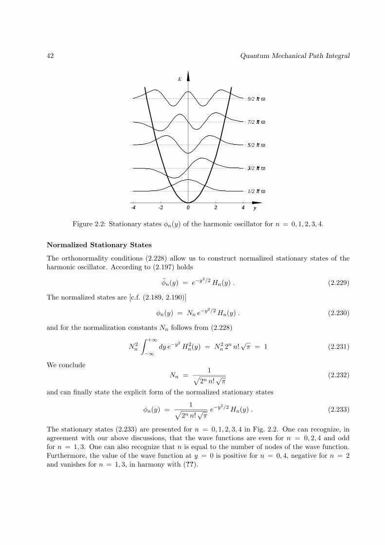
42 Quantum Mechanical Path Integral
-4
-2 0 2 4
E
ω1/2
3/2
5/2
7/2
9/2
ω
ωh
ωh
ωh
h
h
y
Figure 2.2: Stationary states φn(y) of the harmonic oscillator for n = 0, 1, 2, 3, 4.
Normalized Stationary States
The orthonormality conditions (2.228) allow us to construct normalized stationary states of theharmonic oscillator. According to (2.197) holds
φn(y) = e−y2/2Hn(y) . (2.229)
The normalized states are [c.f. (2.189, 2.190)]
φn(y) = Nn e−y2/2Hn(y) . (2.230)
and for the normalization constants Nn follows from (2.228)
N2n
∫ +∞
−∞dy e−y
2H2n(y) = N2
n 2n n!√π = 1 (2.231)
We concludeNn =
1√2n n!
√π
(2.232)
and can finally state the explicit form of the normalized stationary states
φn(y) =1√
2n n!√πe−y
2/2Hn(y) . (2.233)
The stationary states (2.233) are presented for n = 0, 1, 2, 3, 4 in Fig. 2.2. One can recognize, inagreement with our above discussions, that the wave functions are even for n = 0, 2, 4 and oddfor n = 1, 3. One can also recognize that n is equal to the number of nodes of the wave function.Furthermore, the value of the wave function at y = 0 is positive for n = 0, 4, negative for n = 2and vanishes for n = 1, 3, in harmony with (??).
2.5: Propagator for a Quadratic Lagrangian 43
The normalization condition (2.231) of the wave functions differs from that postulated in (2.189)by the Jacobian dx/dy, i.e., by √∣∣∣∣dxdy
∣∣∣∣ =[mω~
] 14. (2.234)
The explicit form of the stationary states of the harmonic oscillator in terms of the position variablex is then, using (2.233) and (2.189)
φn(x) =1√
2n n!
[mωπ~
] 14e−
mωx2
2~ Hn(√mω
~
x) . (2.235)
Completeness of the Hermite Polynomials
The Hermite polynomials are the first members of a large class of special functions which oneencounters in the course of describing stationary quantum states for various potentials and in spacesof different dimensions. The Hermite polynomials are so-called orthonogal polynomials since theyobey the conditions (2.228). The various orthonogal polynomials differ in the spaces Ω ⊂ R overwhich they are defined and differ in a weight function w(y) which enter in their orthonogalityconditions. The latter are written for polynomials pn(x) in the general form∫
Ωdx pn(x) pm(x) w(x) = In δnm (2.236)
where w(x) is a so-called weight function with the property
w(x) ≥ 0, w(x) = 0 only at a discrete set of points xk ∈ Ω (2.237)
and where In denotes some constants. Comparision with (2.228) shows that the orthonogalitycondition of the Hermite polynomials is in complience with (2.236 , 2.237) for Ω = R, w(x) =exp(−x2), and In = 2nn!
√π.
Other examples of orthogonal polynomials are the Legendre and Jacobi polynomials which arisein solving three-dimensional stationary Schrodinger equations, the ultra-spherical harmonics whicharise in n–dimensional Schrodinger equations and the associated Laguerre polynomials which arisefor the stationary quantum states of particles moving in a Coulomb potential. In case of theLegendre polynomials, denoted by P`(x) and introduced in Sect. 5 below [c.f. (5.150 , 5.151, 5.156,5.179] holds Ω = [−1, 1], w(x) ≡ 1, and I` = 2/(2` + 1). In case of the associated Laguerre
polynomials, denoted by L(α)n (x) and encountered in case of the stationary states of the non-
relativistic [see Sect. ??? and eq. ???] and relativistic [see Sect. 10.10 and eq. (10.459] hydrogenatom, holds Ω = [0,+∞[, w(x) = xαe−x, In = Γ(n+α+1)/n! where Γ(z) is the so-called Gammafunction.The orthogonal polynomials pn mentioned above have the important property that they form acomplete basis in the space F of normalizable functions, i.e., of functions which obey∫
Ωdx f2(x) w(x) = <∞ , (2.238)
where the space is endowed with the scalar product
(f |g) =∫
Ωdx f(x) g(x) w(x) = <∞ , f, g ∈ F . (2.239)
44 Quantum Mechanical Path Integral
As a result holds for any f ∈ Ff(x) =
∑n
cn pn(x) (2.240)
wherecn =
1In
∫Ωdx w(x) f(x) pn(x) . (2.241)
The latter identity follows from (2.236). If one replaces for all f ∈ F : f(x) →√w(x) f(x) and,
in particular, pn(x) →√w(x) pn(x) the scalar product (2.239) becomes the conventional scalar
product of quantum mechanics
〈f |g〉 =∫
Ωdx f(x) g(x) . (2.242)
Let us assume now the case of a function space governed by the norm (2.242) and the existence of anormalizable state ψ(y, t) which is stationary under the action of the harmonic oscillator propagator(2.147), i.e., a state for which (2.172) holds. Since the Hermite polynomials form a complete basisfor such states we can expand
ψ(y, t) =∞∑n=0
cn(t) e−y2/2Hn(y) . (2.243)
To be consistent with(2.188, 2.197) it must hold cn(t) = dn exp[−iω(n + 12)t] and, hence, the
stationary state ψ(y, t) is
ψ(y, t) =∞∑n=0
dn exp[−iω(n+12
)t] e−y2/2Hn(y) . (2.244)
For the state to be stationary |ψ(x, t)|2, i.e.,
∞∑n,m=0
d∗ndm exp[iω(m− n)t] e−y2Hn(y)Hm(y) , (2.245)
must be time-independent. The only possibility for this to be true is dn = 0, except for a singlen = no, i.e., ψ(y, t) must be identical to one of the stationary states (2.233). Therefore, the states(2.233) exhaust all stationary states of the harmonic oscillator.
Appendix: Exponential Integral
We want to prove
I =
+∞∫−∞
dy1 . . .
+∞∫−∞
dyn ei∑nj,k yjajkyk =
√(iπ)n
det(a), (2.246)
for det(a) 6= 0 and real, symmetric a, i.e. aT = a. In case of n = 1 this reads∫ +∞
−∞dx ei a x
2=
√i π
a, (2.247)
2.7: Appendix / Exponential Integral 45
which holds for a ∈ C as long as a 6= 0.The proof of (2.246) exploits that for any real, symmetric matrix exists a similarity transformationsuch that
S−1a S = a =
a11 0 . . . 00 a22 . . . 0...
.... . .
...0 0 . . . ann
. (2.248)
where S can be chosen as an orthonormal transformation, i.e.,
STS = 11 or S = S−1 . (2.249)
The akk are the eigenvalues of a and are real. This property allows one to simplify the bilinearform
∑nj,k yjajkyk by introducing new integration variables
yj =n∑k
(S−1)jkyk ; yk =n∑k
Skj yj . (2.250)
The bilinear form in (2.246) reads then in terms of yj
∑nj,k yjajkyk =
n∑j,k
n∑`m
y`Sj`ajkSkmym
=n∑j,k
n∑`m
y`(ST )`jajkSkmym
=n∑j,k
yj ajkyk (2.251)
where, according to (2.248, 2.249)
ajk =n∑l,m
(ST )jlalmSmk . (2.252)
For the determinant of a holds
det(a) =n∏j=1
ajj (2.253)
as well as
det(a) = det(S−1aS) = det(S−1) det(a) , det(S)= (det(S))−1 det(a) det(S) = det(a) . (2.254)
One can conclude
det(a) =n∏j=1
ajj . (2.255)

46 Quantum Mechanical Path Integral
We have assumed det(a) 6= 0. Accordingly, holds
n∏j=1
ajj 6= 0 (2.256)
such that none of the eigenvalues of a vanishes, i.e.,
ajj 6= 0 , for j = 1, 2, . . . , n (2.257)
Substitution of the integration variables (2.250) allows one to express (2.250)
I =
+∞∫−∞
dy1 . . .
+∞∫−∞
dyn
∣∣∣∣det(∂(y1, . . . , yn)∂(y1, . . . , yn)
)∣∣∣∣ ei∑nk akky
2k . (2.258)
where we introduced the Jacobian matrix
J =∂(y1, . . . , yn)∂(y1, . . . , yn)
(2.259)
with elementsJjs =
∂yj∂ys
. (2.260)
According to (2.250) holdsJ = S (2.261)
and, hence,
det(∂(y1, . . . , yn)∂(y1, . . . , yn)
) = det(S) . (2.262)
From (2.249) follows1 = det
(STS
)= ( det S )2 (2.263)
such that one can concludedet S = ±1 (2.264)
One can right then (2.258)
I =
+∞∫−∞
dy1 . . .
+∞∫−∞
dyn ei∑nk akky
2k
=
+∞∫−∞
dy1 eia11y2
1 . . .
+∞∫−∞
dyn eianny2
n =n∏k=1
+∞∫−∞
dyk eiakky
2k (2.265)
which leaves us to determine integrals of the type
+∞∫−∞
dx eicx2
(2.266)

2.7: Appendix / Exponential Integral 47
where, according to (2.257) holds c 6= 0.We consider first the case c > 0 and discuss the case c < 0 further below. One can relate inte-gral (2.266) to the well-known Gaussian integral
+∞∫−∞
dx e−cx2
=√π
c, c > 0 . (2.267)
by considering the contour integral
J =∮γ
dz eicz2
= 0 (2.268)
along the path γ = γ1 +γ2 +γ3 +γ4 displayed in Figure 2.3. The contour integral (2.268) vanishes,since eicz
2is a holomorphic function, i.e., the integrand does not exhibit any singularities anywhere
in C. The contour intergral (2.268) can be written as the sum of the following path integrals
J = J1 + J2 + J3 + J4 ; Jk =∮γk
dz eicz2
(2.269)
The contributions Jk can be expressed through integrals along a real coordinate axis by realizingthat the paths γk can be parametrized by real coordinates x
γ1 : z = x J1 =p∫−pdx eicx
2
γ2 : z = ix+ p J2 =p∫0
i dx eic(ix+p)2
γ3 : z =√i x J3 =
−√
2p∫√
2p
√i dx eic(
√ix)2
= −√i
√2p∫
−√
2p
dx e−cx2
γ4 : z = ix− p J4 =0∫−pi dx eic(ix−p)
2,
for x, p ∈ IR.
(2.270)
Substituting −x for x into integral J4 one obtains
J4 =
0∫p
(−i) dx eic(−ix+p)2
=
p∫0
i dx eic(ix−p)2
= J2 . (2.271)

48 Quantum Mechanical Path Integral
p
Im(z)
Re(z)
-p γ 1
γ 2
γ 3
γ 4
i p
-i p
Figure 2.3: Contour path γ in the complex plain.
We will now show that the two integrals J2 and J4 vanish for p → +∞. This follows from thefollowing calculation
limp→+∞
|J2 or 4| = limp→+∞
|p∫
0
i dx eic(ix+p)2 |
≤ limp→+∞
p∫0
|i| dx |eic(p2−x2)| |e−2cxp| . (2.272)
It holds |eic(p2−x2)| = 1 since the exponent of e is purely imaginary. Hence,
limp→+∞
|J2 or 4| ≤ limp→+∞
p∫0
dx |e−2cxp|
= limp→+∞
1− e−2cp
2 c p= 0 . (2.273)
J2 and J4 do not contribute then to integral (2.268) for p = +∞. One can state accordingly
J =
∞∫−∞
dx eicx2 −
√i
∞∫−∞
dx e−cx2
= 0 . (2.274)
Using 2.267) one has shown then∞∫−∞
dx eicx2
=
√iπ
c. (2.275)
2.7: Appendix / Exponential Integral 49
One can derive the same result for c < 0, if one chooses the same contour integral as (2.268), butwith a path γ that is reflected at the real axis. This leads to
J =
∞∫−∞
dx eicx2
+√−i
−∞∫∞
dx ecx2
= 0 (2.276)
and (c < 0)∞∫−∞
dx eicx2
=
√−iπ−|c|
=
√iπ
c. (2.277)
We apply the above results (2.275, 2.277) to (2.265). It holds
I =n∏k=1
√iπ
akk=
√(iπ)n∏nj=1 ajj
. (2.278)
Noting (2.255) this result can be expressed in terms of the matrix a
I =
√(iπ)n
det(a)(2.279)
which concludes our proof.

50 Quantum Mechanical Path Integral
Chapter 3
The Schrodinger Equation
3.1 Derivation of the Schrodinger Equation
We will consider now the propagation of a wave function ψ(~r, t) by an infinitesimal time step ε. Itholds then according to (2.5)
ψ(~r, t+ ε) =∫
Ωd3r0 φ(~r, t+ ε|~r0, t)ψ(~r0, t) . (3.1)
We will expand the l.h.s. and the r.h.s. of this equation in terms of powers of ε and we willdemonstrate that the terms of order ε require that ψ(~r, t) satisfies a partial differential equation,namely the Schrodinger equation. For many situations, but by no means all, the Schrodingerequation provides the simpler avenue towards describing quantum systems than the path ingralformulation of Section 2. Notable exceptions are non-stationary systems involving time-dependentlinear and quadratic Lagrangians.The propagator in (3.1) can be expressed through the discretization scheme (2.20, 2.21). In thelimit of very small ε it is sufficient to employ a single discretization interval in (2.20) to evaluatethe propagator. Generalizing (2.20) to R3 one obtains then for small ε
φ(~r, t+ ε|~r0, t) =[ m
2πi~ε
] 32 exp
i
~
[m
2(~r − ~r0)2
ε− ε U(~r, t)
]. (3.2)
From this follows
ψ(~r, t+ ε) =∫
Ωd3r0
[ m
2πi~ε
] 32 exp
i
~
[m
2(~r − ~r0)2
ε− ε U(~r, t)
]ψ(~r0, t) . (3.3)
In order to carry out the integration we set ~r0 = ~r + ~s and use ~s as the new integration variable.We will denote the components of ~s by (x1, x2, x3)T . This yields
ψ(~r, t+ ε) =∫ +∞−∞ dx1
∫ +∞−∞ dx2
∫ +∞−∞ dx3
[m
2πi~ε
] 32 ×
× exp(i
~
m
2x2
1 + x22 + x2
3
ε− ε U(~r, t)
)︸ ︷︷ ︸
even in x1, x2, , x3
ψ(~r + ~s, t) . (3.4)
51

52 Schrodinger Equation
It is important to note that the integration is not over ~r, but over ~s = (x1, x2, x3)T , e.g. U(~r, t) is aconstant with respect to this integration. The integration involves only the wave function ψ(~r+~s, t)and the kinetic energy term. Since the latter contributes to (3.4) only for small x2
1 +x22 +x2
3 valueswe expand
ψ(~r + ~s, t) = ψ(~r, t) +3∑j=1
xj∂
∂xjψ(~r, t) +
12
3∑j,k=1
xjxk∂2
∂xj∂xkψ(~r, t) + . . . (3.5)
assuming that only the leading terms contribute, a supposition which will be examined below. Sincethe kinetic energy contribution in (3.4) is even in all three coordinates x1, x2, x3, only terms of theexpansion (3.5) which are even separately in all three coordinates yield non-vanishing contributions.It is then sufficient to consider the terms
ψ(~r, t) ; 12
∑3j=1 x
2j∂2
∂x2jψ(~r, t) ; 1
4
∑3j,k=1 x
2jx
2k
∂4
∂x2j∂x
2kψ(~r, t) ;
112
∑3j=1 x
4j∂4
∂x4jψ(~r, t) ; . . . (3.6)
of the expansion of ψ(~r + ~s, t).Obviously, we need then to evaluate integrals of the type
In(a) =∫ +∞
−∞dxx2n exp
(i a x2
), n = 0, 1, 2 (3.7)
According to (2.36) holds
I0(a) =
√iπ
a(3.8)
Inspection of (3.7) shows
In+1(a) =1i
∂
∂aIn(a). (3.9)
Starting from (3.8) one can evaluate recursively all integrals In(a). It holds
I1(a) =i
2a
√iπ
a; I2(a) = − 3
4a2
√iπ
a, . . . (3.10)
It is now important to note that in case of integral (3.4) one identifies
1a
=2 ε ~m
= O(ε) (3.11)
and, consequently, the terms collected in (3.6) make contributions of the order
O(ε32 ) , O(ε
52 ) , O(ε
72 ) , O(ε
72 ) . (3.12)
Here one needs to note that we are actually dealing with a three-fold integral. According to (3.11)holds [ m
2πi~ε
] 32 ×
[i π
a
] 32
= 1 (3.13)

3.2: Boundary Conditions 53
and one can conclude, using (3.10),
ψ(~r, t+ ε) = exp[− iε~
U(~r, t)] [
ψ(~r, t) +14
2iε~m∇2ψ(~r, t) + O(ε2)
]. (3.14)
This expansion in terms of powers of ε suggests that we also expand
ψ(~r, t+ ε) = ψ(~r, t) + ε∂
∂tψ(~r, t) + O(ε2) (3.15)
and
exp[− iε~
U(~r, t)]
= 1 − iε
~
U(~r, t) + O(ε2) . (3.16)
Inserting this into (3.14) results in
ψ(~r, t) + ε ∂∂tψ(~r, t) = ψ(~r, t) − iε
~
U(~r, t)ψ(~r, t)
+iε
~
~2
2m∇2ψ(~r, t) + O(ε2) . (3.17)
Obviously, this equation is trivially satisfied to order O(ε0). In order O(ε) the equation reads
i~∂
∂tψ(~r, t) =
[− ~
2
2m∇2 + U(~r, t)
]ψ(~r, t) . (3.18)
This is the celebrated time-dependent Schrodinger equation. This equation is often written in theform
i~∂
∂tψ(~r, t) = H ψ(~r, t) (3.19)
where
H = − ~2
2m∇2 + U(~r, t) . (3.20)
3.2 Boundary Conditions
The time-dependent Schrodinger equation is a partial differential equation, 1st order in time, 2ndorder in the spatial variables and linear in the solution ψ(~r, t). The following general remarks canbe made about the solution.Due to its linear character any linear combination of solutions of the time-dependent Schrodingerequation is also a solution.The 1st order time derivative requires that for any solution a single temporal condition needs to bespecified, e.g., ψ(~r, t1) = f(~r). Usually, one specifies the so-called initial condition, i.e., a solutionis thought for t ≥ t0 and the solution is specified at the intial time t0.The 2nd order spatial derivatives require that one specifies also properties of the solution on aclosed boundary ∂Ω surrounding the volume Ω in which a solution is to be determined. We willderive briefly the type of boundary conditions encountered. As we will discuss in Chapter 5 belowthe solutions of the Schrodinger equation are restricted to particular Hilbert spaces H which are

54 Schrodinger Equation
linear vector spaces of functions f(~r) in which a scalar product between two elements f, g ∈ H isdefined as follows
〈f |g〉Ω =∫
Ωd3rf∗(~r)g(~r) (3.21)
This leads one to consider the integral
〈f |H |g〉Ω =∫
Ωd3rf∗(~r) H g(~r) (3.22)
where H is defined in (3.20). Interchanging f∗(~r) and g(~r) results in
〈g|H |f〉Ω =∫
Ωd3r g(~r) Hf∗(~r) . (3.23)
Since H is a differential operator the expressions (3.22) and (3.23), in principle, differ from eachother. The difference between the integrals is
〈g|H |f〉Ω = − 〈g|H |f〉Ω
=∫
Ωd3rf∗(~r)
(− ~
2
2m∇2
)g(~r) −
∫Ωd3rg(~r)
(− ~
2
2m∇2
)f∗(~r)
+∫
Ωd3rf∗(~r)U(~r, t) g(~r) −
∫Ωd3rg(~r)U(~r, t), f∗(~r)
= − ~2
2m
∫Ωd3rf∗(~r)
(∇2
)g(~r) −
∫Ωd3rg(~r)
(∇2
)f∗(~r) (3.24)
Using Green’s theorem1 ∫Ω d
3r(f∗(~r)∇2 g(~r) − g(~r)∇2 f∗(~r)
)=∫∂Ω d~a · ( f∗(~r)∇g(~r) − g(~r)∇f∗(~r) ) (3.25)
one obtains the identity
〈f | H |g〉Ω = 〈g| H |f〉Ω +∫∂Ωd~a · ~P (f∗, g|~r) (3.26)
where∫∂Ω d~a · ~A(~r) denotes an integral over the surface ∂Ω of the volume Ω, the surface elements
d~a pointing out of the surface in a direction normal to the surface and the vector–valued function~A(~r) is taken at points ~r ∈ ∂Ω. In (3.26) the vector–valued function ~P (f∗, g|~r) is called theconcomitant of H and is
~P (f∗, g|~r) = − ~2
2m( f∗(~r)∇g(~r) − g(~r)∇f∗(~r) ) (3.27)
We will postulate below that H is an operator in H which represents energy. Since energy is a realquantity one needs to require that the eigenvalues of the operator H are real and, hence, that H ishermitian2. The hermitian property, however, implies
〈f | H |g〉Ω = 〈g| H |f〉Ω (3.28)1See, for example, Calssical Electrodynamics, 2nd Ed., J. D. Jackson, (John Wiley, New York, 1975), Chapter 1.2The reader is advised to consult a reference text on ‘Linear Algebra’ to follow this argument.
3.3: Particle Flux 55
and, therefore, we can only allow functions which make the differential d~a · ~P (f∗, g|~r) vanish on∂Ω. It must hold then for all f ∈ H
f(~r) = 0 ∀~r, ~r ∈ ∂Ω (3.29)
ord~a · ∇f(~r) = 0 ∀~r, ~r ∈ ∂Ω (3.30)
Note that these boundary conditions are linear in f , i.e., if f and g satisfy these conditions thanalso does any linear combination αf + βg. Often the closed surface of a volume ∂Ω is the unionof disconnected surfaces3 ∂Ωj , i.e., ∂Ω = ∂Ω1 ∩ ∂Ω2 ∩ ∂Ω3 ∩ . . . In this case one can postulateboth conditions (3.29, 3.30) each condition holding on an entire surface ∂Ωj . However, to avoiddiscontinuities in ψ(~r, t) on a single connected surface ∂Ωj only either one of the conditions (3.29,3.30) can be postulated.A most common boundary condition is encountered for the volume Ω = ~R3 in which case onepostulates
lim|~r|→∞
f(~r) = 0 “natural boundary condition” . (3.31)
In fact, in this case also all derivatives of f(~r) vanish at infinity. The latter property stems fromthe fact that the boundary condition (3.31) usually arises when a particle existing in a bound stateis described. In this case one can expect that the particle density is localized in the area where theenergy of the particle exceeds the potential eenrgy, and that the density decays rapidly when onemoves away from that area. Since the total probability of finding the particle anywhere in space is∫
d3r|f(~r)|2 = 1 (3.32)
the wave function must decay for |~r| → ∞ rapidly enough to be square integrable, i.e., obey (3.32),e.g., like exp(−κr), κ > 0 or like r−α, α > 2. In either case does f(~r) and all of its derivativesvanish asymptotically.
3.3 Particle Flux and Schrodinger Equation
The solution of the Schrodinger equation is the wave function ψ(~r, t) which describes the state ofa particle moving in the potential U(~r, t). The observable directly linked to the wave function isthe probability to find the particle at position ~r at time t, namely, |ψ(~r, t)|2. The probability toobserve the particle anywhere in the subvolume ω ⊂ Ω is
p(ω, t) =∫ωd3r |ψ(~r, t)|2 . (3.33)
The time derivative of p(ω, t) is
∂tp(ω, t) =∫ωd3r [ψ∗(~r, t)∂tψ(~r, t) + ψ(~r, t)∂tψ∗(~r, t) ] . (3.34)
3An example is a volume between two concentric spheres, in which case ∂Ω1 is the inner sphere and ∂Ω2 is theouter sphere.

56 Schrodinger Equation
Using (3.19) and its conjugate complex4
− i~ ∂∂tψ∗(~r, t) = H ψ∗(~r, t) (3.35)
yields
i~∂tp(ω, t) =∫ωd3r
[ψ∗(~r, t) H ψ(~r, t) − ψ(~r, t) H ψ∗(~r, t)
]. (3.36)
According to (3.26, 3.27) this can be written
i~∂tp(ω, t) =∫∂ωd~a · ~P (ψ∗(~r, t), ψ(~r, t)~r, t) . (3.37)
If one applies this identity to ω = Ω one obtains according to (3.29, 3.30) ∂tp(Ω, t) = 0. Accord-ingly the probability to observe the particle anywhere in the total volume Ω is constant. A naturalchoice for this constant is 1. One can multiply the solution of (3.18) by any complex number andaccordingly one can define ψ(~r, t) such that∫
Ωd3r|ψ(~r, t)|2 = 1 (3.38)
holds. One refers to such solution as normalized. We will assume in the remainder of this Sectionthat the solutions discussed are normalized. Note that for a normalized wave function the quantity
ρ(~r, t) = |ψ(~r, t)|2 (3.39)
is a probability density with units 1/volume.The surface integral (3.37) can be expressed through a volume integral according to∫
∂ωd~a · ~A(~r) =
∫ωd3r∇ · ~A(~r) (3.40)
One can rewrite then (3.37) ∫ωd3r
(∂tρ(~r, t) + ∇ ·~j(~r, t)
)= 0 (3.41)
where~j(~r, t) = ~P (ψ∗, ψ|~r, t) . (3.42)
Using (3.27) one can express this
~j(~r, t) =~
2mi[ψ(~r, t)∇ψ∗(~r, t) − ψ∗(~r, t)∇ψ(~r, t) ] . (3.43)
Since (3.41) holds for any volume ω ⊂ Ω one can conclude
∂tρ(~r, t) + ∇ ·~j(~r, t) = 0 . (3.44)4Note that the Hamiltonian H involves only real terms.

3.4: Free Particle 57
The interpretation of ~j(~r, t) is that of density flux. This follows directly from an inspection ofEq. (3.41) written in the form
∂t
∫ωd3r ρ(~r, t) = −
∫∂ωd~a ·~j(~r, t) . (3.45)
Obviously, ~j(~r, t) gives rise to a descrease of the total probability in volume ω due to the disap-pearence of probability density at the surface ∂ω. Note that ~j(~r, t) points in the direction to theoutside of volume ω.It is of interest to note from (3.43) that any real wave function ψ(~r, t) has vanishing flux anywhere.One often encounters wave functions of the type
φ(~r) = f(~r) ei~k·~r , for f(~r) ∈ R. (3.46)
The corresponding flux is
~j(~r) =~~k
mf2(~r) , (3.47)
i.e., arises solely from the complex factor exp(i~k · ~r). Such case arose in Sect. 2 for a free parti-cle [c.f. (2.48, 2.71)], and for particles moving in a linear [c.f. (2.105, 2.125)] and in a quadratic[c.f. (2.148, 2.167)] potential. In Sect. 2 we had demonstrated that a factor exp(ipoxo/~) inducesa motion of 1-dimensional wave packets such that po/m corresponds to the initial velocity. Thisfinding is consistent with the present evaluation of the particle flux: a factor exp(ipoxo/~) gives riseto a flux po/m, i.e., equal to the velocity of the particle. The generalization to three dimenisonsimplies then that the factor exp(i~k ·~r) corresponds to an intial velocit ~~k/m and a flux of the samemagnitude.
3.4 Solution of the Free Particle Schrodinger Equation
We want to consider now solutions of the Schrodinger equation (3.18) in Ω∞ = R3 in the case
U(~r, t) = 0
i~∂
∂tψ(~r, t) = − ~
2
2m∇2 ψ(~r, t) (3.48)
which describes the motion of free particles. One can readily show by insertion into (3.48) that thegeneral solution is of the form
ψ(~r, t) = [2π]−32
∫Ω∞
d3k φ(~k) exp(i(~k · ~r − ωt)
)(3.49)
where the dispersion relationship holds
ω =~k2
2m. (3.50)
Obviously, the initial condition at ψ(~r, t0) determines φ(~k). Equation (3.49) reads at t = t0
ψ(~r, t0) = [2π]−32
∫Ω∞
d3k φ(~k) exp(i(~k · ~r − ωt0)
). (3.51)
58 Schrodinger Equation
The inverse Fourier transform yields
φ(~k) = [2π]−32
∫Ω∞
d3r0 exp(−i~k · ~r0)ψ(~r0, t0) . (3.52)
We have not specified the spatial boundary condition in case of (3.49). The solution as stated isdefined in the infinte space Ω∞ = R
3. If one chooses the initial state f(~r) defined in (3.51) tobe square integrable it follows according to the properties of the Fourier–transform that ψ(~r, t) asgiven by (3.49) is square integrable at all subsequent times and, hence, that the “natural boundarycondition” (3.31) applies. The ensuing solutions are called wave packets.
Comparision with Path Integral Formulation
One can write solution (3.49, 3.51, 3.52) above
ψ(~r, t) =∫
Ω∞
d3r0 φ(~r, t|~r0, t0)ψ(~r0, t0) (3.53)
where
φ(~r, t|~r0, t0) =[
12π
]3 ∫Ω∞
d3k exp(i~k · (~r − ~r0) − i
~
~2k2
2m(t − t0)
). (3.54)
This expression obviously has the same form as postulated in the path integral formulation of Quan-tum Mechanics introduced above, i.e., in (2.5). We have identified then with (3.54) an alternativerepresentation of the propagator (2.47). In fact, evaluating the integral in (3.54) yields (2.47). Toshow this one needs to note
12π
∫ +∞
−∞dk1 exp
(i~k1(x − x0) − i
~
~2k2
1
2m(t − t0)
)=[
m
2πi~(t− t0)
] 12
exp[im
2~(x− x0)2
t− t0
]. (3.55)
This follows from completion of the square
i~k1(x − x0) − i
~
~2k2
1
2m(t − t0)
= −i ~(t− to)2m
[k1 −
m
~
x− xot− to
]2
+i
~
m
2(x− xo)2
t− to(3.56)
and using (2.247).Below we will generalize the propagator (3.54) to the case of non-vanishing potentials U(~r), i.e.,derive an expression similar to (3.54) valid for this case. The general form for this propagatorinvolves an expansion in terms of a complete set of eigenfunctions as in (3.114) and (4.70) derivedbelow for a particle in a box and the harmonic oscillator, respectively. In case of the harmonocoscillator the expansion can be stated in a closed form given in (4.81)

3.4: Free Particle 59
Free Particle at Rest
We want to apply solution (3.49, 3.52) to the case that the initial state of a 1-dimensional freeparticle ψ(x0, t) is given by (??). The 1-dimensional version of (3.53, 3.54) is
ψ(x, t) =∫ +∞
−∞dx0 φ(x, t|x0, t0)ψ(x0, t) (3.57)
where
φ(x, t|x0, t0) =1
2π
∫ +∞
−∞dk exp
(ik (x − x0) − i
~
~2k2
2m(t − t0)
). (3.58)
Integration over x0 leads to the integral∫ +∞
−∞dx0exp
(−ikx0 +
i
~
pox0 −x2
0
2δ2
)=√
2πδ2 exp(−
(k − po~
)2δ2
2
)(3.59)
which is solved through completion of the square in the exponent [c.f. (3.55, (3.56)]. The remainingintegration over k leads to the integral∫ +∞
−∞ dk exp[ikx − 1
2 (k − po~
)2 δ2 − i ~k2
m (t− t0)]
=???? (3.60)
Combining (3.57–3.60) yields with t0 = 0
ψ(x, t) =
[1 − i ~t
mδ2
1 + i ~tmδ2
] 14[
1πδ2 (1 + ~2t2
m2δ4 )
] 14
× (3.61)
× exp
[−
(x − pom t)2
2δ2(1 + ~2t2
m2δ4 )(1 − i
~t
mδ2) + i
po~
x − i
~
p2o
2mt
].
a result which is identical to the expression (??) obtained by means of the path integral propagator(2.46). We have demonstrated then in this case that the Schrodinger formulation of QuantumMechanics is equivalent to the Feynman path integral formulation.
Stationary States
We consider now solutions of the time-dependent Schrodinger equation (3.19, 3.20) which are ofthe form
ψ(~r, t) = f(t)φ(~r) . (3.62)
We will restrict the space of allowed solutions to a volume Ω such that the functions also make theconcomitant (3.27) vanish on the surface ∂Ω of Ω, i.e., the functions obey boundary conditions ofthe type (3.29, 3.30). Accordingly, the boundary conditions are
φ(~r) = 0 ∀~r, ~r ∈ ∂Ω (3.63)
ord~a · ∇φ(~r) = 0 ∀~r, ~r ∈ ∂Ω (3.64)

60 Schrodinger Equation
and affect only the spatial wave function φ(~r). As pointed out above, a common case is Ω = Ω∞and the ‘natural boundary condition’ (3.31). We will demonstrate that solutions of the type (3.62)do exist and we will characterize the two factors of the solution f(t) and φ(~r). We may note inpassing that solutions of the type (3.62) which consist of two factors, one factor depending only onthe time variable and the other only on the space variables are called separable in space and time.It is important to realize that the separable solutions (3.62) are special solutions of the time-dependent Schrodinger equation, by no means all solutions are of this type. In fact, the solutions(3.62) have the particular property that the associated probability distributions are independentof time. We want to demonstrate this property now. It follows from the observation that for thesolution space considered (3.27) holds and, hence, according to (3.42) the flux ~j(~r, t) vanishes onthe surface of ∂Ω. It follows then from (3.45) that the total probability∫
Ωd3r ρ(~r, t) =
∫Ωd3r |ψ(~r, t)|2 = |f(t)|2
∫Ωd3r |φ(~r)|2 (3.65)
is constant. This can hold only if |f(t)| is time-independent, i.e., if
f(t) = eiα, α ∈ R . (3.66)
One can conclude that the probability density for the state (3.62) is
|ψ(~r, t)|2 = |φ(~r)|2 , (3.67)
i.e., is time-independent. One calls such states stationary states.In order to further characterize the solution (3.62) we insert it into (3.19). This yields an expression
g1(t)h1(~r) = g2(t)h2(~r) (3.68)
where g1(t) = i~∂tf(t), g2(t) = f(t), h1(~r) = φ(~r), and h2(~r) = H φ(~r). The identity (3.68) canhold only for all t and all ~r if g1(t) = E g2(t) and E h1(~r) = h2(~r) for some E ∈ C. We mustpostulate therefore
∂t f(t) = E f(t)H φ(~r) = E φ(~r) . (3.69)
If these two equations can be solved simultaneously a solution of the type (3.62) exists.It turns out that a solution for f(t) can be found for any E, namely
f(t) = f(0) exp(− i
~
E t
). (3.70)
The task of finding solutions φ(~r) which solve (3.69) is called an eigenvalue problem. We willencounter many such problems in the subsequent Sections. At this point we state without proofthat, in general, for the eigenvalue problems in the confined function space, i.e., for functionsrequired to obey boundary conditions (3.63, 3.64), solutions exist only for a set of discrete Evalues, the eigenvalues of the operator H. At this point we will accept that solutions φ(~r) of thetype (3.69) exist, however, often only for a discrete set of values En, n = 1, 2, . . . We denote thecorresponding solution by φE(~r). We have then shown that
ψ(~r, t) = f(0) exp(− i
~
E
)φE(~r) where H φE(~r) = E φE(~r) . (3.71)
3.4: Free Particle 61
is a solution of the time-dependent Schrodinger equation (3.19, 3.20).According to (3.66) E must be real. We want to prove now that the eigenvalues E which arise inthe eigenvalue problem (3.71) are, in fact, real. We start our proof using the property (3.28) forthe special case that f and g in (3.28) both represent the state φE(~r), i.e.,∫
Ωd3r φ∗E(~r) H φE(~r) =
∫Ωd3r φE(~r) H φ∗E(~r) . (3.72)
According to (3.71) this yields
E
∫Ωd3r φ∗E(~r)φE(~r) = E∗
∫Ωd3r φE(~r)φ∗E(~r) . (3.73)
from which follows E = E∗ and, hence, E ∈ R. We will show in Section 5 that E can beinterprerted as the total energy of a stationary state.
Stationary State of a Free Particle
We consider now the stationary state of a free particle described by
ψ(~r, t) = exp(− i~
E t
)φE(~r) , − ~
2
2m∇2 φ(~r) = E φ(~r) . (3.74)
The classical free particle with constant energy E > 0 moves without bounds in the space Ω∞. Asa result we cannot postulate in the present case that wave functions are localized and normalizable.We will wave this assumption as we always need to do later whenever we deal with unboundparticles, e.g. particles scattered of a potential.The solution φE(~r) corresponding to the eigenvalue problem posed by (3.74) is actually best labelledby an index ~k, ~k ∈ R3
φ~k(~r) = N exp(i~k · ~r
),~
2k2
2m= E . (3.75)
One can ascertain this statement by inserting the expression for φ~k(~r) into the eigenvalue problem
posed in (3.74) using ∇exp(i~k · ~r
)= i~k exp
(i~k · ~r
). The resulting total energy values E are
positive, a property which is to be expected since the energy is purely kinetic energy which, ofcourse, should be positive.The corresponding stationary solution
ψ(~r, t) = exp(− i~
~2k2
2mt
)exp
(i~k · ~r
)(3.76)
has kinetic energy ~2k2/2m. Obviously, one can interpret then ~k as the magnitude of the momen-tum of the particle. The flux corresponding to (3.76) according to (3.43) is
~j(~r, t) = |N |2 ~~k
m. (3.77)
Noting that ~k can be interpreted as the magnitude of the momentum of the particle the flux isequal to the velocity of the particle ~v = ~~k/m multiplied by |N |2.
62 Schrodinger Equation
3.5 Particle in One-Dimensional Box
As an example of a situation in which only bound states exist in a quantum system we consider thestationary states of a particle confined to a one-dimensional interval [−a, a] ⊂ R assuming that thepotential outside of this interval is infinite. We will refer to this as a particle in a one-dimensional‘box’.
Setting up the Space F1 of Proper Spatial Functions
The presence of the infinite energy wall is accounted for by restricting the spatial dependence of thesolutions to functions f(x) defined in the domain Ω1 = [−a, a] ⊂ R which vanish on the surface∂Ω1 = −a, a, i.e.,
f ∈ F1 = f : [−a, a] ⊂ R → R, f continuous, f(±a) = 0 (3.78)
Solutions of the Schrodinger Equation in F1
The time–dependent solutions satisfy
i~∂tψ(x, t) = − ~2
2md2
dx2ψ(x, t) . (3.79)
The stationary solutions have the form ψ(x, t) = exp(−iEt/~)φE(x) where φE(x) is determinedby
− ~2
2md2
dx2φE(x) = E φE(x) , φ(±a) = 0 . (3.80)
We note that the box is symmetric with respect to the origin. We can expect, hence, that thesolutions obey this symmetry as well. We assume, therefore, two types of solutions, so-called evensolutions obeying φ(x) = φ(−x)
φ(e)E (x) = A coskx ,
~2k2
2m= E (3.81)
and so-called odd solutions obeying φ(x) = −φ(−x)
φ(o)E (x) = A sinkx; ,
~2k2
2m= E . (3.82)
One can readily verify that (3.81, 3.82) satisfy the differential equation in (3.80).The boundary conditions which according to (3.80) need to be satisfied are
φ(e,o)E (a) = 0 and φ
(e,o)E (−a) = 0 (3.83)
The solutions (3.81, 3.82) have the property that either both boundary conditions are satisfied ornone. Hence, we have to consider only one boundary condition, let say the one at x = a. It turnsout that this boundary condition can only be satisfied for a discrete set of k–values kn, n ∈ N. Incase of the even solutions (3.81) they are
kn =nπ
2a, n = 1, 3, 5 . . . (3.84)

3.5: Particle in One-Dimensional Box 63
since for such kncos(kna) = cos
(nπa2a
)= cos
(nπ2
)= 0 . (3.85)
In case of the odd solutions (3.82) only the kn–values
kn =nπ
2a, n = 2, 4, 6 . . . (3.86)
satisfy the boundary condition since for such kn
sin(kna) = sin(nπa
2a
)= sin
(nπ2
)= 0 . (3.87)
(Note that, according to (3.86), n is assumed to be even.)
The Energy Spectrum and Stationary State Wave Functions
The energy values corresponding to the kn–values in (3.84, 3.86), according to the dispersionrelationships given in (3.81, 3.82), are
En =~
2π2
8ma2n2 , n = 1, 2, 3 . . . (3.88)
where the energies for odd (even) n–values correspond to the even (odd) solutions given in (3.81)and (3.82), respectively, i.e.,
φ(e)n (a;x) = An cos
nπx
2a, n = 1, 3, 5 . . . (3.89)
andφ(o)n (a;x) = An sin
nπx
2a, n = 2, 4, 6 . . . . (3.90)
The wave functions represent stationary states of the particle in a one-dimensional box. The wavefunctions for the five lowest energies En are presented in Fig. (3.1). Notice that the number ofnodes of the wave functions increase by one in going from one state to the state with the nexthigher energy En. By counting the number of their nodes one can determine the energy orderingof the wave functions.It is desirable to normalize the wave functions such that∫ +a
−adx |φ(e,o)
n (a;x)|2 = 1 (3.91)
holds. This condition implies for the even states
|An|2∫ +a
−adx cos2nπx
2a= |An|2 a = 1 , n = 1, 3, 5 . . . (3.92)
and for the odd states
|An|2∫ +a
−adx sin2nπx
2a= |An|2 a = 1 , n = 2, 4, 6 . . . (3.93)
The normalization constants are then
An =
√1a. (3.94)
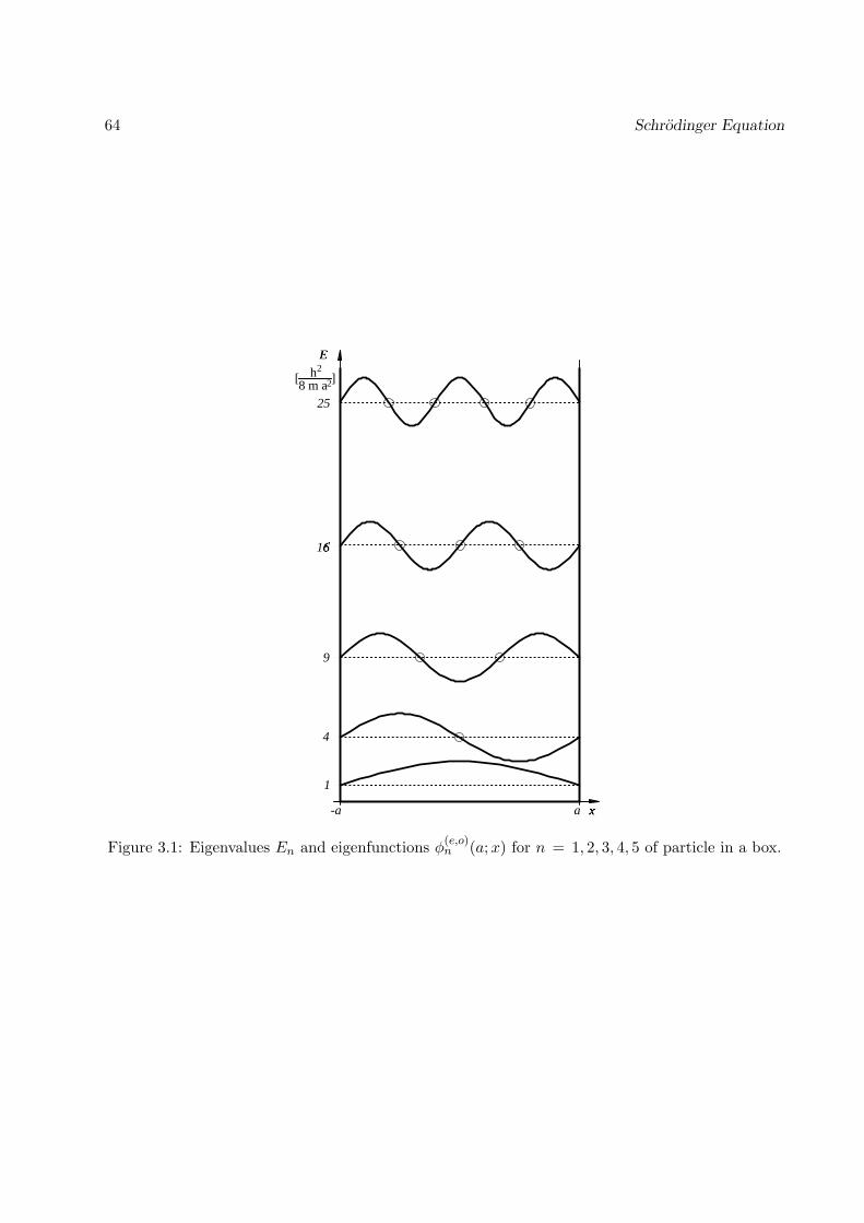
64 Schrodinger Equation
1
4
9
16
25
-a a x
E
[ ]h2
8 m a2
Figure 3.1: Eigenvalues En and eigenfunctions φ(e,o)n (a;x) for n = 1, 2, 3, 4, 5 of particle in a box.
3.5: Particle in One-Dimensional Box 65
The Stationary States form a Complete Orthonormal Basis of F1
We want to demonstrate now that the set of solutions (3.89, 3.90, 3.94)
B1 = φn(a;x) , n = 1, 2, 3, . . . (3.95)
where
φn(a;x) =
√1a
cosnπx2a for n = 1, 3, 5 . . .sinnπx2a for n = 2, 4, 6 . . .
(3.96)
together with the scalar product5
〈f |g〉Ω1 =∫ +a
−adxf(x) g(x) , f, g ∈ F1 (3.97)
form an orthonormal basis set, i.e., it holds
〈φn|φm〉Ω1 = δnm . (3.98)
The latter property is obviously true for n = m. In case of n 6= m we have to consider three cases,(i) n,m both odd, (ii) n,m both even, and (iii) the mixed case. The latter case leads to integrals
〈φn|φm〉Ω1 =1a
∫ +a
−adx cos
nπx
2asin
mπx
2a. (3.99)
Since in this case the integrand is a product of an even and of an odd function, i.e., the integrandis odd, the integral vanishes. Hence we need to consider only the first two cases. In case of n,modd, n 6= m, the integral arises
〈φn|φm〉Ω1 = 1a
∫ +a−a dx cosnπx2a cosmπx2a =
1a
∫ +a−a dx
[cos (n−m)πx
2a + cos (n+m)πx2a
](3.100)
The periods of the two cos-functions in the interval [−a, a] are N, N ≥ 1. Obviously, the integralsvanish. Similarly, one obtains for n,m even
〈φn|φm〉Ω1 = 1a
∫ +a−a dx sinnπx2a sinmπx2a =
1a
∫ +a−a dx
[cos (n−m)πx
2a − cos (n+m)πx2a
](3.101)
and, hence, this integral vanishes, too.Because of the property (3.98) the elements of B1 must be linearly independent. In fact, for
f(x) =∞∑n=1
dn φn(a;x) (3.102)
holds according to (3.98)
〈f |f〉Ω1 =∞∑n=1
d2n . (3.103)
5We will show in Section 5 that the property of a scalar product do indeed apply. In particular, it holds:〈f |f〉Ω1 = 0 → f(x) ≡ 0.

66 Schrodinger Equation
f(x) ≡ 0 implies 〈f |f〉Ω1 = 0 which in turn implies dn = 0 since d2n ≥ 0. It follows that B1
defined in (3.95) is an orthonormal basis.We like to show finally that the basis (3.95) is also complete, i.e., any element of the function spaceF1 defined in (3.78) can be expressed as a linear combination of the elements of B1 defined in(3.95, 3.96). Demonstration of completeness is a formidable task. In the present case, however,such demonstration can be based on the theory of Fourier series. For this purpose we extend thedefinition of the elements of F1 to the whole real axis through
f : R → R ; ~f(x) = f([x+ a]a − a) (3.104)
where [y]a = ymod2a. The functions f are periodic with period 2a. Hence, they can be expandedin terms of a Fourier series, i.e., there exist real constants an, n = 0, 1, 2, . . . and bn, n = 1, 2, . . .such that
f =∞∑n=0
an cosnπx
2a+
∞∑n=1
an sinnπx
2a(3.105)
The functions f corresponding to the functions in the space F1 have zeros at x = ±ma, m =1, 3, 5 . . . Accordingly, the coefficients an, n = 2, 4, . . . and bn, n = 1, 3, . . . in (3.105) must vanish.This implies that only the trigonometric functions which are elements of B1 enter into the Fourierseries. We have then shown that any f corresponding to elements of F1 can be expanded in termsof elements in B1. Restricting the expansion (3.105) to the interval [−a, a] yields then also anexpansion for any element in F1 and B1 is a complete basis for F1.
Evaluating the Propagator
We can now use the expansion of any initial wave function ψ(x, t0) in terms of eigenfunctionsφn(a;x) to obtain an expression for ψ(x, t) at times t > t0. For this purpose we expand
ψ(x, t0) =∞∑n=1
dn φn(a;x) . (3.106)
Using the orthonormality property (3.98) one obtains∫ +a
−adx0φm(a;x0)ψ(x0, t0) = dm . (3.107)
Inserting this into (3.106) and generalizing to t ≥ t0 one can write
ψ(x, t) =∞∑n=1
φn(a;x) cn(t)∫ +a
−adx0φn(a;x0)ψ(x0, t0) (3.108)
where the functions cn(t) are to be determined from the Schrodinger equation (3.79) requiring theinitial condition
cn(t0) = 1 . (3.109)
Insertion of (3.108) into the Schrodinger equation yields∑∞n=1 φn(a;x) ∂tcn(t)
∫ +a−a dx0φn(a;x0)ψ(x0, t0) =∑∞
n=1
(− i~En)φn(a;x) cn(t)
∫ +a−a dx0φn(a;x0)ψ(x0, t0) . (3.110)

3.5: Particle in One-Dimensional Box 67
Multiplying both sides by φm(a;x) and integrating over [−a, a] yields, according to (3.98),
∂t cm(t) = − i~
Em cm(t) , cm(t0) = 1 . (3.111)
The solutions of these equations which satisfy (3.109) are
cm(t) = exp(− i~
Em (t − t0)). (3.112)
Equations (3.108, 3.112) determine now ψ(x, t) for any initial condition ψ(x, t0). This solution canbe written
ψ(x, t) =∫ +a
−adx0 φ(x, t|x0, t0)ψ(x0, t0) (3.113)
where
φ(x, t|x0, t0) =∞∑n=1
φn(a;x) exp(− i~
En (t − t0))φn(a;x0) . (3.114)
This expression has the same form as postulated in the path integral formulation of QuantumMechanics introduced above, i.e., in (2.5). We have identified then with (3.114) the representationof the propagator for a particle in a box with infinite walls.It is of interest to note that φ(x, t|x0, t0) itself is a solution of the time-dependent Schrodingerequation (3.79) which lies in the proper function space (3.78). The respective initial conditionis φ(x, t0|x0, t0) = δ(x − x0) as can be readily verified using (3.113). Often the propagatorφ(x, t|x0, t0) is also referred to as a Greens function. In the present system which is composedsolely of bound states the propagator is given by a sum, rather than by an integral (3.54) as in thecase of the free particle system which does not exhibit any bound states.Note that the propagator has been evaluated in terms of elements of a particular function space F1,the elements of which satisfy the appropriate boundary conditions. In case that different boundaryconditions hold the propagator will be different as well.
Example of a Non-Stationary State
As an illustration of a non-stationary state we consider a particle in an initial state
ψ(x0, t0) =[
12πσ2
] 14
exp(− x2
0
2σ2+ i k0 x0
), σ =
a
4, k0 =
15a. (3.115)
This initial state corresponds to the particle being localized initially near x0 = 0 with a velocityv0 = 15~/ma in the direction of the positive x-axis. Figure 3.2 presents the probability distributionof the particle at subsequent times. One can recognize that the particle moves first to the left andthat near the right wall of the box interference effects develop. The particle moves then to theleft, being reflected at the right wall. The interference pattern begins to ‘smear out’ first, but thecollision with the left wall leads to new interference effects. The last frame shows the wave frontreaching again the right wall and the onset of new interference.

68 Schrodinger Equation
-a a
1π σ
|Ψ|2
k = 15a
-a a
1π σ
|Ψ|2
-a a
1π σ
|Ψ|2
-a a
1π σ
|Ψ|2
-a a
1π σ
|Ψ|2
-a a
1π σ
|Ψ|2
-a a
1π σ
|Ψ|2
-a a
1π σ
|Ψ|2
-a a
1π σ
|Ψ|2
-a a
1π σ
|Ψ|2
h2m a2
t = 0.00
h2m a2
t = 0.48
h2m a2
t = 0.96
h2m a2
t = 1.92h2
m a2t = 2.16
h2m a2
t = 1.68
h2m a2
t = 1.20
h2m a2
t = 0.72
h2m a2
t = 0.24
h2m a2
t = 1.44
Figure 3.2: Stroboscopic views of the probability distribution |ψ(x, t)|2 for a particle in a boxstarting in a Gaussian distribution with momentum 15~/a.
3.6: Particle in Three-Dimensional Box 69
Summary: Particle in One-Dimensional Box
We like to summarize our description of the particle in the one-dimensional box from a point ofview which will be elaborated further in Section 5. The description employed a space of functionsF1 defined in (3.78). A complete basis of F1 is given by the infinite set B1 (3.95). An importantproperty of this basis and, hence, of the space F1 is that the elements of the basis set can beenumerated by integer numbers, i.e., can be counted. We have defined in the space F1 a scalarproduct (3.97) with respect to which the eigenfunctions are orthonormal. This property allowed usto evaluate the propagator (3.114) in terms of which the solutions for all initial conditions can beexpressed.
3.6 Particle in Three-Dimensional Box
We consider now a particle moving in a three-dimensional rectangular box with side lengths2a1, 2a2, 2a3. Placing the origin at the center and aligning the x1, x2, x3–axes with the edgesof the box yields spatial boundary conditions which are obeyed by the elements of the functionspace
F3 = f : Ω → R, f continuous, f(x1,x2,x3) = 0 ∀ (x1,x2,x3)T ∈ ∂ . (3.116)
where Ω is the interior of the box and ∂Ω its surface
Ω = [−a1, a1]⊗ [−a2, a2]⊗ [−a3, a3] ⊂ R3
∂Ω = (x1, x2, x3)T ∈ Ω, x1 = ±a1 ∪ (x1, x2, x3)T ∈ Ω, x2 = ±a2∪ (x1, x2, x3)T ∈ Ω, x3 = ±a3 . (3.117)
We seek then solutions of the time-dependent Schrodinger equation
i~∂tψ(x, t) = H ψ(x1, x2, x3, t) , H = − ~2
2m(∂2
1 + ∂22 + ∂2
3
)(3.118)
which are stationary states. The corresponding solutions have the form
ψ(x1, x2, x3, t) = exp(− i~
E t
)φE(x1, x2, x3) (3.119)
where φE(x1, x2, x3) is an element of the function space F3 defined in (3.116) and obeys the partialdifferential equation
H φE(x1, x2, x3) = E φE(x1, x2, x3) . (3.120)
Since the Hamiltonian H is a sum of operators O(xj) each dependent only on a single variable, i.e.,H = O(x1) +O(x2) +O(x3), one can express
φ(x1, x2, x3) =3∏j=1
φ(j)(xj) (3.121)
where
− ~2
2m∂2j φ
(j)(xj) = Ej φ(j)(xj) , φ(j)(±aj) = 0 , j = 1, 2, 3 (3.122)

70 Schrodinger Equation
and E1 + E2 + E3 = E. Comparing (3.122) with (3.80) shows that the solutions of (3.122) aregiven by (3.96) and, hence, the solutions of (3.120) can be written
φ(n1,n2,n3)(a1, a2, a3;x1, x2, x3) = φn1(a1;x1)φn2(a2;x2)φn3(a3;x3)n1, n2, n3 = 1, 2, 3, . . . (3.123)
and
E(n1,n2,n3) =~
2π2
8m
(n2
1
a21
+n2
2
a22
+n2
3
a23
), n1, n2, n3 = 1, 2, 3, . . . (3.124)
The same considerations as in the one-dimensional case allow one to show that
B3 = φ(n1,n2,n3)(a1, a2, a3;x1, x2, x3) , n1, n2, n3 = 1, 2, 3, . . . (3.125)
is a complete orthonormal basis of F3 and that the propagator for the three-dimensional box is
φ(~r, t|~r0, t0) =∞∑
n1,n2,n3=1
φ(n1,n2,n3)(a1, a2, a3;~r) (3.126)
exp(− i~
E(n1n2n3) (t − t0))φ(n1,n2,n3)(a1, a2, a3;~r0) .
Symmetries
The three-dimensional box confining a particle allows three symmetry operations that leave the boxunchanged, namely rotation by π around the x1, x2, x3–axes. This symmetry has been exploitedin deriving the stationary states. If two or all three orthogonal sides of the box have the samelength further symmetry operations leave the system unaltered. For example, if all three lengthsa1, a2, a3 are identical, i.e., a1 = a2 = a3 = a then rotation around the x1, x2, x3–axes by π/2also leaves the system unaltered. This additional symmetry is also reflected by degeneracies in theenergy levels. The energies and corresponding degeneracies of the particle in the three-dimensionalbox with all side lengths equal to 2a are given in the following Table:
n1 n2 n3 E/[~2π2/8ma2] degeneracy1 1 1 3 single1 1 2 6 three-fold1 2 2 9 three-fold1 1 3 11 three-fold2 2 2 12 single1 2 3 14 six-fold2 2 3 17 three-fold1 1 4 18 three-fold2 3 3 22 three-fold3 3 3 27 single1 1 5 27 three-fold
One can readily verify that the symmetry of the box leads to three-fold and six-fold degeneracies.Such degeneracies are always a signature of an underlying symmetry. Actually, in the present case

3.6: Particle in Three-Dimensional Box 71
‘accidental’ degeneracies also occur, e.g., for (n1, n2, n3) = (3, 3, 3) (1, 1, 5) as shown in the Tableabove. The origin of this degeneracy is, however, the identity 32 + 32 + 32 = 12 + 12 + 52.One particular aspect of the degeneracies illustrated in the Table above is worth mentioning. Weconsider the degeneracy of the energy E122 which is due to the identity E122 = E212 = E221. Anylinear combination of wave functions
φ(~r) = αφ(1,2,2)(a, a, a;~r) + β φ(2,1,2)(a, a, a;~r) + γ φ(2,2,1)(a, a, a;~r) (3.127)
obeys the stationary Schrodinger equation H φ(~r) = E122 φ(~r). However, this linear combinationis not necessarily orthogonal to other degeneraste states, for example, φ(1,2,2)(a, a, a;~r). Hence,in case of degenerate states one cannot necessarily expect that stationary states are orthogonal.However, in case of an n–fold degeneracy it is always possible, due to the hermitian character ofH, to construct n orthogonal stationary states6.
6This is a result of linear algebra which the reader may find in a respective textbook.

72 Schrodinger Equation

Chapter 4
Linear Harmonic Oscillator
The linear harmonic oscillator is described by the Schrodinger equation
i ~ ∂t ψ(x, t) = H ψ(x, t) (4.1)
for the Hamiltonian
H = − ~2
2m∂2
∂x2+
12mω2x2 . (4.2)
It comprises one of the most important examples of elementary Quantum Mechanics. There are sev-eral reasons for its pivotal role. The linear harmonic oscillator describes vibrations in molecules andtheir counterparts in solids, the phonons. Many more physical systems can, at least approximately,be described in terms of linear harmonic oscillator models. However, the most eminent role of thisoscillator is its linkage to the boson, one of the conceptual building blocks of microscopic physics.For example, bosons describe the modes of the electromagnetic field, providing the basis for itsquantization. The linear harmonic oscillator, even though it may represent rather non-elementaryobjects like a solid and a molecule, provides a window into the most elementary structure of thephysical world. The most likely reason for this connection with fundamental properties of matteris that the harmonic oscillator Hamiltonian (4.2) is symmetric in momentum and position, bothoperators appearing as quadratic terms.We have encountered the harmonic oscillator already in Sect. 2 where we determined, in the contextof a path integral approach, its propagator, the motion of coherent states, and its stationary states.In the present section we approach the harmonic oscillator in the framework of the Schrodingerequation. The important role of the harmonic oscillator certainly justifies an approach from twoperspectives, i.e., from the path integral (propagotor) perspective and from the Schrodinger equa-tion perspective. The path integral approach gave us a direct route to study time-dependentproperties, the Schrodinger equation approach is suited particularly for stationary state properties.Both approaches, however, yield the same stationary states and the same propagator, as we willdemonstrate below.The Schrodinger equation approach will allow us to emphasize the algebraic aspects of quantumtheory. This Section will be the first in which an algebraic formulation will assume center stage.In this respect the material presented provides an important introduction to later Sections usingLie algebra methods to describe more elementary physical systems. Due to the pedagodical natureof this Section we will link carefully the algebraic treatment with the differential equation methodsused so far in studying the Schrodinger equation description of quantum systems.
73

74 Linear Harmonic Oscillator
In the following we consider first the stationary states of the linear harmonic oscillator and laterconsider the propagator which describes the time evolution of any initial state. The stationary statesof the harmonic oscillator have been considered already in Chapter 2 where the corresponding wavefunctions (2.235) had been determined. In the framework of the Schrodinger equation the stationarystates are solutions of (4.1) of the form ψ(x, t) = exp(−iEt/~)φE(x, t) where
H φE(x) = E φE(x) . (4.3)
Due to the nature of the harmonic potential which does not allow a particle with finite energy tomove to arbitrary large distances, all stationary states of the harmonic oscillator must be boundstates and, therefore, the natural boundary conditions apply
limx→±∞
φE(x) = 0 . (4.4)
Equation (4.3) can be solved for any E ∈ R, however, only for a discrete set of E values can theboundary conditions (4.4) be satisfied. In the following algebraic solution of (4.3) we restrict theHamiltonian H and the operators appearing in the Hamiltonian from the outset to the space offunctions
N1 = f : R → R, f ∈ C∞, limx→±∞
f(x) = 0 (4.5)
where C∞ denotes the set of functions which together with all of their derivatives are continuous.It is important to keep in mind this restriction of the space, in which the operators used below,act. We will point out explicitly where assumptions are made which built on this restriction. Ifthis restriction would not apply and all functions f : R → R would be admitted, the spectrum ofH in (4.3) would be continuous and the eigenfunctions φE(x) would not be normalizable.
4.1 Creation and Annihilation Operators
The Hamiltonian operator (4.2) can be expressed in terms of the two operators
p =~
i
d
dx, x = x (4.6)
the first being a differential operator and the second a multiplicative operator. The operators acton the space of functions N1 defined in (4.5). The Hamiltonian H can be expressed in terms of theoperators acting on the space (4.5)
H =1
2mp2 +
12mω2 x2 (4.7)
which is why these operators are of interest to us.The cardinal property exploited below, beside the representation (4.7) of the Hamiltonian, is thecommutation property
[p, x] =~
i11 (4.8)
which holds for any position and momentum operator. This property states that p and x obey analgebra in which the two do not commute, however, the commutator has a simple form. In order
4.1: Creation and Annihilation Operators 75
to derive (4.8) we recall that all operators act on functions in N1 and, hence, the action of [p, x]on such functions must be considered. One obtains
[p, x] f(x) =~
i
d
dxx f(x) − x
~
i
d
dxf(x) =
~
if(x) =
~
i11 f(x) . (4.9)
From this follows (4.8).Our next step is an attempt to factorize the Hamiltonian (4.7) assuming that the factors are easierto handle than the Hamiltonian in yielding spectrum and eigenstates. Being guided by the identityfor scalar numbers
(b− ic)(b+ ic) = b2 − i(cb− bc) + c2 = b2 + c2 (4.10)
we define
a+ =√mω
2~x − i√
2m~ωp , a− =
√mω
2~x +
i√2m~ω
p . (4.11)
The reader may note that we have attempted, in fact, to factor H/~ω. Since a+ and a− areoperators and not scalars we cannot simply expect that the identy (4.10) holds for a+ and a− since[a−, a+] = a−a+ − a+a− does not necessarily vanish. In fact, the commutator property (4.8)implies
[a−, a+] = 11 . (4.12)
To prove this commutation property we determine using (4.11)
a−a+ =mω
2~x2 +
12m~ω
p2 +i
2~[p, x] . (4.13)
(4.7) and (4.8) yield
a−a+ =1~ω
H +12
11 . (4.14)
Similarly one can show
a+a− =1~ω
H − 12
11 . (4.15)
(4.14) and (4.15) together lead to the commutation property (4.12).Before we continue we like to write (4.14, 4.15) in a form which will be useful below
H = ~ω a−a+ − ~ω
211 (4.16)
H = ~ω a+a− +~ω
211 . (4.17)
We also express a+ and a− directly in terms of the coordinate x and the differential operator ddx
a+ =√mω
2~x −
√~
2mωd
dx, a− =
√mω
2~x +
√~
2mωd
dx. (4.18)
It is of interest to note that the operators a+ and a− are real differential operators.

76 Linear Harmonic Oscillator
Relationship between a+ and a−
The operators a+ and a− are related to each other by the following property which holds for allfunctions f, g ∈ N1 ∫ +∞
−∞dx f(x) a+ g(x) =
∫ +∞
−∞dx g(x) a− f(x) . (4.19)
This property states that the operators a+ and a− are the adjoints of each other. The propertyfollows directly from (??). Using (??) we like to state (4.19) in the form1
〈f |a+g〉Ω∞ = 〈g|a−f〉Ω∞ . (4.20)
In the following we will determine the spectrum of H and its eigenstates. The derivation will bebased solely on the properties (4.12, 4.16, 4.17, 4.19).
a+ and a− as Ladder Operators
The operators a+ and a− allow one to generate all stationary states of a harmonic oscillator onceone such state φE(x)
H φE(x) = E φE(x) (4.21)
is available. In fact, one obtains using (4.16, 4.17, 4.21)
H a− φE(x) = ( ~ω a−a+ − ~ω
211 ) a− φE(x)
= a− ( ~ω a+a− +~ω
211 − ~ω 11 )φE(x)
= a− ( H − ~ω )φE(x)= (E − ~ω ) a− φE(x) . (4.22)
Similarly one can show using again (4.16, 4.17, 4.21)
H a+ φE(x) = ( ~ω a+a− +~ω
211 ) a+ φE(x)
= a+ ( ~ω a−a+ − ~ω
211 + ~ω 11 )φE(x)
= a+ ( H + ~ω )φE(x)= (E + ~ω ) a+ φE(x) . (4.23)
Together, it holds that for a stationary state φE(x) of energy E defined through (4.21) a−φE(x) isa stationary state of energy E − ~ω and a+φE(x) is a stationary state of energy E + ~ω.The results (4.22, 4.23) can be generalized to m-fold application of the operators a+ and a−
H (a+)m φE(x) = (E + m ~ω )(a+)m
φE(x)
H (a−)m φE(x) = (E − m ~ω )(a−)m
φE(x) . (4.24)1This property states that the operators in the function space N1 are the hermitian conjugate of each other. This
property of operators is investigated more systematically in Section 5.

4.2: Ground State 77
One can use these relationships to construct an infinite number of stationary states by stepping upand down the spectrum in steps of ±~ω. For obvious reasons one refers to a+ and a− as ladderoperators. Another name is creation (a+) and annihilation (a−) operators since these operatorscreate and annihilate vibrational quanta ~ω. There arise, however, two difficulties: (i) one needs toknow at least one stationary state to start the construction; (ii) the construction appears to yieldenergy eigenvalues without lower bounds when, in fact, one expects that E = 0 should be a lowerbound. It turns out that both difficulties can be resolved together. In fact, a state φ0(x) whichobeys the property
a− φ0(x) = 0 (4.25)
on one side would lead to termination of the sequence E0 + m, m ∈ Z when m is decreased, onthe other side such a state is itself an eigenstate of H as can be shown using (4.17)
H φ0(x) = ( ~ω a+a− +~ω
211 )φ0(x) =
12~ω φ0(x) . (4.26)
Of course, the solution φ0(x) of (4.25) needs to be normalizable in order to represent a bound stateof the harmonic oscillator, i.e., φ0(x) should be an element of the function space N1 defined in(4.5).The property (??) has an important consequence for the stationary states φE(x). Let φE(x) andφE′(x) be two normalized stationary states corresponding to two different energies E,E′, E 6= E′.For f(x) = φE(x) and g(x) = φE′(x) in (??) follows (Note that according to (??) the eigenvalueE is real.)
0 = 〈φE |HφE′〉Ω∞ − 〈φE′ |HφE〉Ω∞ = (E′ − E ) 〈φE |φE′〉Ω∞ . (4.27)
Since E 6= E′ one can conclude〈φE |φE′〉Ω∞ = 0 . (4.28)
4.2 Ground State of the Harmonic Oscillator
A suitable solution of (4.25) can, in fact, be found. Using (4.6, 4.11) one can rewrite (4.25)(d
dy+ y
)φ0(y) = 0 (4.29)
where
y =√mω
~
x . (4.30)
Assuming that φ0(y) does not vanish anywhere in its domain ]−∞,+∞[ one can write (4.29)
1φ0(y)
d
dyφ0(y) = =
d
dylnφ0(y) = − y , (4.31)
the solution of which islnφ0(y) = −1
2y2 + c0 (4.32)
for some constant c0 or
φ0(y) = c0 exp(−1
2y2
). (4.33)

78 Linear Harmonic Oscillator
This solution is obviously normalizable. The conventional normalization condition
〈φ0|φ0〉Ω∞ = 1 (4.34)
reads ∫ +∞
−∞dx |φ0(x)|2 = |c0|2
∫ +∞
−∞dx exp
(−mωx
2
2~
)= |c0|2
√π~
mω. (4.35)
The appropriate ground state is
φ0(x) =[mωπ~
] 14 exp
(−mωx
2
2~
). (4.36)
Since the first order differential equation (4.25) admits only one solution there is only one set ofstates with energy E + m ~ω, m ∈ Z which properly terminate at some minimum value E +m0 ~ω ≥ 0. We recall that according to (4.26) the energy value associated with this state is 1
2~ω.This state of lowest energy is called the ground state of the oscillator. The set of allowed energiesof the oscillator according to (4.24) can then be written as follows
En = ~ω (n +12
) , n = 0, 1, 2, . . . (4.37)
It is most remarkable that the energy 12~ω of the ground state is larger than the lowest classically
allowed energy E = 0. The reason is that in the Hamiltonian (4.2) there are two competingcontributions to the energy, the potential energy contribution which for a state δ(x), i.e., a stateconfined to the minimum corresponding to the classical state of lowest energy, would yield a van-ishing contribution, and the kinetic energy contribution, which for a narrowly localized state yieldsa large positive value. The ground state (4.36) assumes a functional form such that both termstogether assume a minimum value. We will consider this point more systematically in Section 5.
4.3 Excited States of the Harmonic Oscillator
Having obtained a suitable stationary state with lowest energy, we can now construct the stationarystates corresponding to energies (4.37) above the ground state energy, i.e., we construct the statesfor n = 1, 2, . . ., the so-called excited states. For this purpose we apply the operator a+ to theground state (4.36) n times. Such states need to be suitably normalized for which purpose weintroduce a normalization constant c′n
φn(x) = c′n(a+)n
φ0(x) , n = 0, 1, 2, . . . (4.38)
These states correspond to the energy eigenvalues (4.39), i.e., it holds
H φn(x) = ~ω (n +12
)φn(x) , n = 0, 1, 2, . . . (4.39)
We notice that the ground state wave function φ0(x) as well as the operators (a+)n are real. Wecan, therefore, choose the normalization constants c′n and the functions φn(x) real as well.

4.3: Excited States 79
We need to determine now the normalization constants c′n. To determine these constants we adopta recursion scheme. For n = 0 holds c′0 = 1. We consider then the situation that we have obtaineda properly normalized state φn(x). A properly normalized state φn+1(x) is then of the form
φn+1(x) = αn a+ φn(x) (4.40)
for some real constant αn which is chosen to satisfy
〈φn+1|φn+1〉Ω∞ = α2n 〈a+φn|a+φn〉Ω∞ = 1 . (4.41)
Employing the adjoint property (4.20) yields
α2n 〈φn|a−a+φn〉Ω∞ = 1 . (4.42)
Using (4.14) together with H φn(x) = ~ω(n+ 12)φn(x) leads to the condition (note that we assumed
φn(x) to be normalized)
α2n (n + 1 ) 〈φn|a−a+φn〉Ω∞ = α2
n (n + 1 ) = 1 (4.43)
From this follows αn = 1/√n+ 1 and, according to (4.40),
a+ φn(x) =√n+ 1φn+1(x) . (4.44)
One can conclude then that the stationary states of the oscillator are described by the functions
φn(x) =1√n!
(a+)n
φ0(x) , n = 0, 1, 2, . . . (4.45)
We like to note that these functions according to (4.28) and the construction (4.40–4.45) form anorthonormal set, i.e., they obey
〈φn|φn′〉 = δnn′ , n, n′ = 0, 1, 2, . . . . (4.46)
According to (4.24) holds in analogy to (4.40)
φn−1(x) = βn a− φn(x) (4.47)
for some suitable constants βn. Since a− is a real differential operator [see (4.18)] and since theφn(x) are real functions, βn must be real as well. To determine βn we note using (4.20)
1 = 〈φn−1|φn−1〉Ω∞ = β2n 〈a−φn|a−φn〉Ω∞ = β2
n 〈φn|a+a−φn〉Ω∞ . (4.48)
Equations (4.15 , 4.39) yield1 = β2
n n 〈φn|φn〉Ω∞ = β2n n . (4.49)
From this follows βn = 1/√n and, according to (4.47),
a− φn(x) =√nφn−1(x) . (4.50)
Repeated application of this relationship yields
φn−s(x) =
√(n− s)!n!
(a−)sφn(x) . (4.51)

80 Linear Harmonic Oscillator
Evaluating the Stationary States
We want to derive now an analytical expression for the stationary state wave functions φn(x)defined through (4.39). For this purpose we start from expression (4.45), simplifying the calculation,however, by introducing the variable y defined in (4.30) and employing the normalization∫ +∞
−∞dy φ2
n(y) = 1 (4.52)
This normalization of the wave functions differs from that postulated in (4.35) by a constant,n–independent factor, namely the square root of the Jacobian dx/dy, i.e., by√∣∣∣∣dxdy
∣∣∣∣ =[mω~
] 14. (4.53)
We will later re-introduce this factor to account for the proper normalization (4.35) rather than(4.52).In terms of y the ground state wave function is
φ0(y) = π−14 e−
y2
2 (4.54)
and a+ is
a+ =1√2
(y − d
dy
). (4.55)
The eigenstates of the Hamiltonian are then given by
φn(y) =1√
2n n!√πe−
y2
2 ey2
2
(y − d
dy
)ne−
y2
2 . (4.56)
Relationship to Hermite Polynomials
We want to demonstrate now that the expression (4.56) can be expressed in terms of Hermitepolynomials Hn(y) introduced in Sect. 2.7 and given, for example, by the Rodrigues formula (2.200).We will demonstrate below the identity
Hn(y) = ey2
2
(y − d
dy
)ne−
y2
2 (4.57)
such that one can write the stationary state wave functions of the harmonic oscillator
φn(y) =1√
2n n!√πe−
y2
2 Hn(y) . (4.58)
This result agrees with the expression (2.233) derived in Sect. 2.7. It should be noted that thenormalization (4.28) of the ground state and the definition (4.57) which includes the factor 1/
√n!
according to Eqs. (4.40–4.46) yields a set of normalized states.
4.4: Propagator 81
To verify the realtionship between the definition (4.57) of the hermite polynomials and the definitiongiven by (2.200) we need to verify(
y − d
dy
)ne−
y2
2 = (−1)n ey2
2dn
dyne−y
2. (4.59)
which implies
Hn(y) = (−1)n ey2 dn
dyne−y
2(4.60)
and, hence, the Rodrigues formula (2.200).We prove (4.59) by induction noting first that (4.59) holds for n = 0, 1, and showing then that theproperty also holds for n+ 1 in case it holds for n, i.e.,
g(y) = (−1)n+1 ey2
2dn+1
dyn+1e−y
2=(y − d
dy
)n+1
e−y2
2 . (4.61)
One can factor g(y) and employ (4.59) as follows
g(y) = −ey2
2d
dye−
y2
2 (−1)n ey2
2dn
dyne−y
2
= −ey2
2d
dye−
y2
2
(y − d
dy
)ne−
y2
2 . (4.62)
Denoting f(y) = (y − d/dy)exp(−y2/2) and employing
d
dye−
y2
2 f(y) = −y e−y2
2 f(y) + e−y2
2d
dyf(y) (4.63)
one obtains
g(y) =(y − d
dy
)f(y) (4.64)
which implies that (4.61) and, therefore, (4.59) hold.
4.4 Propagator for the Harmonic Oscillator
We consider now the solution of the time-dependent Schrodinger equation of the harmonic oscillator(4.1, 4.2) for an arbitrary initial wave function ψ(x0, t0). Our derivation will follow closely theprocedure adopted for the case of a ‘particle in a box’ [see Eqs. (3.106–3.114)]. For the sake ofnotational simplicity we employ initially the coordinate y as defined in (4.30) and return later tothe coordinate x.Starting point of our derivation is the assumption that the initial condition can be expanded interms of the eigenstates φn(y) (4.39)
ψ(y0, t0) =∞∑n=0
dn φn(y0) . (4.65)

82 Linear Harmonic Oscillator
Such expansion is possible for any f(y0) = ψ(y0, t0) which is an element of N1 defined in (4.5),a supposition which is not proven here2. Employing orthogonality condition (4.46) the expansioncoefficients dn are
dn =∫ +∞
−∞dy0 ψ(y0, t0)φn(y0) . (4.66)
One can extend expansion (4.65) to times t ≥ t0 through insertion of time-dependent coefficientscn(t1)
ψ(y, t1) =∞∑n=0
dn φn(y) cn(t) (4.67)
for which according to (3.108–3.112) and (4.39) holds
cn(t1) = exp(−i ω (n +
12
) ( t1 − t0 )). (4.68)
Altogether one can express then the solution
ψ(y, t1) =∫ +∞
−∞dy0 φ(y, t|y0, t0)ψ(y0, t) (4.69)
where
φ(y, t1|y0, t0) =∞∑n=0
φn(y)φn(y0) tn+ 12 , t = e−iω(t1−t0) (4.70)
is the propagator of the linear harmonic oscillator. We want to demonstrate now that this propaga-tor is identical to the propagator (2.147) for the harmonic iscillator determined in Sect. sec:harm.In order to prove the equivalence of (4.70) and (2.147) we employ the technique of generatingfunctions as in Sect. 2.7. For this purpose we start from the integral representation (2.225) whichallows one to derive a generating function for products of Hermite polynomials which can be appliedto the r.h.s. of (4.70). We consider for this purpose the following expression for |t| < 1
w(y, y0, t) =∞∑n=0
Hn(y)e−y2/2Hn(y0)e−y
20/2
2n n!√π
tn . (4.71)
Applying (??) to express Hn(y) and Hn(y0) yields
w(y, y0, t) = π−3/2 exp(y2
2+y2
0
2
)∫ +∞
−∞du
∫ +∞
−∞dv
exp(−2tuv)︷ ︸︸ ︷∞∑n=0
1n!
(−2tuv )n ×
× exp(−u2 − v2 + 2iyu + 2iy0v ) . (4.72)
2A demonstration of this property can be found in Special Functions and their Applications by N.N.Lebedev(Prentice Hall, Inc., Englewood Cliffs, N.J., 1965) Sect. 4.15, pp. 68; this is an excellent textbook from which wehave borrowed heavily in this Section.

4.4: Propagator 83
Carrying out the sum on the r.h.s. one obtains
w(y, y0, t) = π−3/2 exp(y2
2+y2
0
2
) ∫ +∞
−∞dv exp(−v2 + 2iy0v ) ×
×∫ +∞
−∞du exp(−u2 − 2u(tv − iy) )︸ ︷︷ ︸√πexp( t2v2− 2iytv− y2)
. (4.73)
The incomplete Gaussian integral∫ +∞
−∞dx e−a
2x2− 2bx =√π
aeb
2/a2, Re a2 > 0 (4.74)
applied once results in
w(y, y0, t) = π−1 exp(−y
2
2+y2
0
2
) ∫ +∞
−∞dv exp(−(1− t2) v2 − 2i (yt − y0) v) . (4.75)
Applying (4.74) a second time yields finally together with the definition (4.71) of w(y, y0, t)
1√π(1−t2)
exp[−1
2(y2 + y20) 1 + t2
1− t2 + 2 y y0t
1− t2
]=∑∞
n=0Hn(y)e−y
2/2 Hn(y0)e−y20/2
2n n!√π
tn . (4.76)
One can express this in terms of the stationary states (4.58) of the harmonic oscillator∞∑n=0
φn(y)φn(y0) tn =1√
π(1− t2)exp
[−1
2(y2 + y2
0)1 + t2
1 − t2+ 2 y y0
t
1 − t2
]. (4.77)
The sum in (4.70) is, indeed, identical to the generating function (4.77), i.e., it holds
φ(y, t1|y0, t0) =1√
2 i π F (t1, t0)exp
[i
2(y2 + y2
0)G(t1, t0) − i y y01
F (t1, t0)
](4.78)
where
F (t1, t0) =1 − e−2iω(t1−t0)
2 i e−iω(t1−t0)= sinω(t1 − t0) (4.79)
and
G(t1, t0) = i1 + e−2iω(t1−t0)
1 − e−2iω(t1−t0)=
cosω(t1 − t0)sinω(t1 − t0)
. (4.80)
We can finally express the propagator (4.78) in terms of the coordinates x and x0. This requiresthat we employ (4.30) to replace y and y0 and that we multiply the propagator by
√mω/~, i.e.,
by a factor 4√mω/~ for both φn(y) and φn(y0). The resulting propagator is
φ(x, t|x0, t0) =[
mω
2iπ~ sinω(t1 − t0)
] 12
×
exp
imω
2~ sinω(t1 − t0)[
(x2 + x20) cosω(t1 − t0) − 2xx0
]. (4.81)
This result agrees with the propagator (2.147) derived by means of the path integral description.
84 Linear Harmonic Oscillator
4.5 Working with Ladder Operators
In the last section we have demonstrated the use of differential equation techniques, the use ofgenerating functions. We want to introduce now techniques based on the ladder operators a+ anda−. For the present there is actually no pressing need to apply such techniques since the techniquesborrowed from the theory of differential equations serve us well in describing harmonic oscillatortype quantum systems. The reason for introducing the calculus of the operators a+ and a− is thatthis calculus proves to be useful for the description of vibrations in crystals, i.e., phonons, and ofthe modes of the quantized electromagnetic field; both quantum systems are endowed with a largenumber of modes, each corresponding to a single harmonic oscillator of the type studied presentlyby us. It is with quantum electrodynamics and solid state physics in mind that we cease theopportunity of the single quantum mechanical harmonic oscillator to develop a working knowledgefor a+ and a− in the most simple setting.To put the following material in the proper modest perspective we may phrase it as an approachwhich rather than employing the coordinate y and the differential operator d/dy uses the operators
a+ =1√2
(y − d
dy
), a− =
1√2
(y +
d
dy
). (4.82)
Obviously, one can express y =√
2(a− + a+) and d/dy =√
2(a− − a+) and, hence, the approachesusing y, d/dy and a+, a− must be equivalent.
Calculus of Creation and Annihilation Operators
We summarize first the key properties of the operators a+ and a−
[a−, a+] = 11a− φ0(y) = 0a+ φn(y) =
√n+ 1φn+1(y)
a− φn(y) =√nφn−1(y)
〈a− f |g〉Ω∞ = 〈f |a+ g〉Ω∞ . (4.83)
We note that these properties imply
φn(y) = (a+)nφ0(y)/√n! . (4.84)
We will encounter below functions of a+ and a−, e.g., f(a+). Such functions are defined forf : R → R in case that the Taylor expansion
f(y) =∞∑ν=0
f (ν)(0)ν!
yν (4.85)
is convergent everywhere in R. Here f (ν)(y0) denotes the ν-th derivative of f(y) taken at y = y0.In this case we define
f(a+) =∞∑ν=0
f (ν)(0)ν!
(a+)ν (4.86)

4.5: Working with Creation and Annihilation Operators 85
and similarly for f(a−). The following important property holds
a− f(a+) = f (1)(a+) + f(a+) a− . (4.87)
In particular,a− f(a+)φ0(y) = f (1)(a+)φ0(y) (4.88)
which follows from a− φo(y) = 0. We note
a− f(a+) = [a−, f(a+)] + f(a+) a− (4.89)
which implies that in order to prove (4.87, 4.88) we need to show actually
[a−, f(a+)] = f (1)(a+) . (4.90)
To prove (4.90) we show that (4.90) holds for any function fn(a+) = (a+)n which is a power ofa+. The convergence of the Taylor expansion ascertains then that (4.90) holds for f(a+).We proceed by induction noticing first that (4.90) holds for f0 and for f1. The first case is trivial,the second case follows from
[a−, f1(a+)] = [a−, a+] = 11 = f(1)1 (a+) . (4.91)
Let us assume that (4.90) holds for fn. For fn+1 follows then
[a−, fn+1(a+)] = [a−, (a+)na+] = (a+)n [a−, a+] + [a−, (a+)n] a+
= (a+)n 11 + n (a+)n−1a+ = (n+ 1) (a+)n (4.92)
Since any function f(y) in the proper function space N1 can be expanded
f(y) =∞∑n=0
dn φn(y) =∞∑n=0
dn(a+)n√n!
φ0(y) (4.93)
one can reduce all operators acting on some proper state function by operators acting on the stateφ0(y). Hence, property (4.88) is a fundamental one and will be used in the following, i.e., we willonly assume operator functions acting on φ0(y). As long as the operators act on φ0(y) one canstate then that a− behaves like a differential operator with respect to functions f(a+). Note thatan immediate consequence of (4.88) is
(a−)n f(a+)φo(y) = f (n)(a+)φ0(y) . (4.94)
We like to state the following property of the functions f(a±)
〈f(a−)φ|ψ〉 = 〈φ|f(a+)ψ〉 . (4.95)
This identity follows from (4.83) and can be proven for all powers fn by induction and then inferredfor all proper functions f(a±).An important operator function is the exponential function. An example is the so-called shiftoperator exp(ua−). It holds
eua−f(a+)φ0(y) = f(a+ + u)φ0(y) . (4.96)
86 Linear Harmonic Oscillator
To prove this property we expand exp(ua−)
∞∑ν=0
uν
ν!(a−)ν f(a+)φ0(y) =
∞∑ν=0
uν
ν!f (ν)(a+)φ0(y) = f(a+ + u)φ0(y) . (4.97)
An example in which (4.96) is applied is
eua−eva
+φ0(y) = ev (a+ +u) φ0(y) = euv eva
+φ0(y) . (4.98)
The related operators exp[va+ ± v∗a−] play also an important role. We assume in the followingderivation, without explicitly stating this, that the operators considered act on φ0(y). To expressthese operators as products of operators exp(va+) and exp(v∗a−) we consider the operator C(u) =exp(uza+) exp(uz∗a−) where u ∈ R, z ∈ C, zz∗ = 1 and determine its derivative
ddu C(u) = za+euza
+euz∗a− + euza
+z∗a− euz
∗a− =(za+ + z∗a−
)euza
+euz∗a− −
[z∗a−, euza
+]euz∗a− (4.99)
Using (4.90) and zz∗ = 1 we can write this
ddu C(u) =
(za+ + z∗a−
)euza
+euz∗a− − u euza
+euz∗a− =(
za+ + z∗a− − u)C(u) . (4.100)
To solve this differential equation we define C(u) = D(u) exp(−u2/2) which leads to
d
duD(u) =
(za+ + z∗a−
)D(u) (4.101)
C(u) obviously obeys C(0) = 11. This results in D(0) = 11 and, hence, the solution of (4.101)is D(u) = exp(uza+ + uz∗a−). One can conclude then using the definition of C(u) and definingv = uz
eva+ + v∗a−φ0(y) = e
12vv∗ eva
+ev∗a−φ0(y) . (4.102)
Similarly, one obtainseva
+− v∗a−φ0(y) = e−12vv∗ eva
+e− v
∗a−φ0(y) (4.103)
eva+ + v∗a−φ0(y) = e−
12vv∗ ev
∗a− eva+φ0(y) (4.104)
eva+− v∗a−φ0(y) = e
12vv∗ e−v
∗a− e va+φ0(y) . (4.105)
Below we will use the operator identity which follows for the choice of v = α in (4.105)
eαa+−α∗a−φ0(y) = e
αα∗2 e−α
∗a− eαa+φ0(y) . (4.106)
Applying (4.98) for u = −α∗ and v = α yields
e−α∗a− eαa
+φ0(y) = e−αα
∗eαa
+φ0(y) . (4.107)
This together with (4.106) yields
eαa+−α∗a−φ0(y) = e−
αα∗2 eαa
+φ0(y) . (4.108)

4.5: Working with Creation and Annihilation Operators 87
Generating Function in Terms of a+
We want to demonstrate now that generating functions are as useful a tool in the calculus of theladder operators as they are in the calculus of differential operators. We will derive the equivalentof a generating function and use it to rederive the values Hn(0) and the orthonormality propertiesof φn(y).We start from the generating function (??) and replace according to (4.58) the Hermite polynomialsHn(y) by the eigenstates φn(y)
e2yt− t2 = π14
∞∑n=0
(√
2t)n√n!
ey2/2 φn(y) (4.109)
Using (4.84) and defining√
2t = u one can write then
π−14 exp
(−y
2
2+√
2u y − u2
2
)=
∞∑n=0
un
n!(a+)n φ0(y) (4.110)
or
π−14 exp
(−y
2
2+√
2u y − u2
2
)= eua
+φ0(y) . (4.111)
This expression, in the ladder operator calculus, is the equivalent of the generating function (??).We want to derive now the values Hn(0). Setting y = 0 in (4.111) yields
π−14 exp
(− u
2
2
)= eua
+φ0(0) . (4.112)
Expanding both sides of this equation and using (4.84, 4.58) one obtains
π−14
∞∑ν=0
(−1)νu2ν
2νν!=
∞∑ν=0
uν√ν!φν(0) =
∞∑ν=0
uν√2ν√π ν!
Hν(0) (4.113)
Comparision of all terms on the l.h.s. and on the r.h.s. provide the same values for Hn(0) as providedin Eq. (??).Similarly, we can reproduce by means of the generating function (4.111) the orthonormality prop-erties of the wave functions φn(y). For this purpose we consider
〈eua+φ0|eva
+φ0〉 = 〈φ0|eua
−eva
+φ0〉 (4.114)
where we have employed (4.95). Using (4.98) and again (4.95) one obtains
〈eua+φ0|eva
+φ0〉 = 〈φ0|euv eva
+φ0〉 = euv 〈eva− φ0|φ0〉 = euv (4.115)
where the latter step follows after expansion of eva−
and using a− φ0(y) = 0. Expanding r.h.s. andl.h.s. of (4.115) and using (4.84) yields
∞∑ν,µ=0
uµ vν√µ!ν!〈φµ|φν〉 =
∞∑µ=0
uµ vµ
µ!(4.116)
from which follows by comparision of each term on both sides 〈φµ|φν〉 = δµ ν , i.e., the expectedorthonormality property.
88 Linear Harmonic Oscillator
4.6 Momentum Representation for the Harmonic Oscillator
The description of the harmonic oscillator provided so far allows one to determine the probabilitydensity P (x) of finding an oscillator at position x. For example, for an oscillator in a stationarystate φn(x) as given by (2.235), the probability density is
P (x) = |φn(x)|2 . (4.117)
In this section we want to provide a representation for the harmonic oscillator which is most naturalif one wishes to determine for a stationary state of the system the probability density P (p) of findingthe system at momentum p. For this purpose we employ the Schrodinger equation in the momentumrepresentation.In the position representation the wave function is a function of x, i.e., is given by a function ψ(x);the momentum and position operators are as stated in (4.6) and the Hamiltonian (4.7) is given by(4.2). In the momentum representation the wave function is a function of p, i.e., is given by thefunction ψ(p); the momentum and position operators are
p = p , x = i~d
dp, (4.118)
and the Hamiltonian (4.7) is
H =1
2mp2 − m~2ω2
2d2
dp2. (4.119)
Accordingly, the time-independent Schrodinger equation for the oscillator can be written(−mω
2~
2
2d2
dp2+
12m
p2
)φE(p) = E φE(p) . (4.120)
Multiplying this equation by 1/m2ω2 yields(− ~
2
2md2
dp2+
12mω2 p2
)φE(p) = E φE(p) (4.121)
whereE = E /m2ω2 , ω = 1 /m2ω . (4.122)
For a solution of the Schrodinger equation in the momentum representation, i.e., of (4.121), wenote that the posed eigenvalue problem is formally identical to the Schrodinger equation in theposition representation as given by (4.2, 4.3). The solutions can be stated readily exploiting theearlier results. The eigenvalues, according to (4.37), are
En = ~ω (n + 12
) , n = 0, 1, 2, . . . (4.123)
or, using (4.122),En = ~ω (n + 1
2)) , n = 0, 1, 2, . . . (4.124)
As to be expected, the eigenvalues are identical to those determined in the position representation.The momentum representation eigenfunctions are, using (2.235),
φn(p) =(−i)n√
2n n!
[mω
π~
] 14
exp(−mωp
2
2~
)Hn(
√mω
~
p) . (4.125)

4.6: Momentum Representation 89
or with (4.122)
φn(p) =(−i)n√
2n n!
[1
πm~ω
] 14
exp(− p2
2m~ω
)Hn(
√1
m~ωp) . (4.126)
Normalized eigenfunctions are, of course, defined only up to an arbitrary phase factor eiα, α ∈ R;this allowed us to introduce in (4.125, 4.126) a phase factor (−i)n.We can now state the probability density Pn(p) for an oscillator with energy En to assume momen-tum p. According to the theory of the momentum representation holds
Pn(p) = |φn(p)|2 (4.127)
or
Pn(p) =1
2n n!
[1
πm~ω
] 12
exp(− p2
m~ω
)H2n(
√1
m~ωp) . (4.128)
We may also express the eigenstates (4.126) in terms of dimensionless units following the procedureadopted for the position representation where we employed the substitution (4.30) to obtain (4.58).Defining k =
√mω/~ p or
k =
√1
m~ωp (4.129)
one obtains, instead of (4.126),
φn(k) =(−i)n√2n n!
√πe−
k2
2 Hn(k) . (4.130)
We want to finally apply the relationship
φn(p) =1√2π
∫ +∞
−∞dx exp(−ipx/~)φn(x) (4.131)
in the present case employing dimensionless units. From (4.30) and (4.129) follows
k y = p x / ~ (4.132)
and, hence,
φn(k) =1√2π
∫ +∞
−∞dy exp(−iky)φn(y) (4.133)
where we note that a change of the normalization of φn(y) [c.f. (4.30) and (2.235)] absorbs thereplacement dx → dy, i.e., the Jacobian. This implies the property of Hermite polynomials
(−i)n e−k2
2 Hn(k) =∫ +∞
−∞dy exp(−iky) e−
y2
2 Hn(y) (4.134)
Exercise 4.6.1: Demonstrate the validity of (4.134), i.e., the correctness of the phase factors(−i)n, through direct integration. Proceed as follows.

90 Linear Harmonic Oscillator
(a) Prove first the property
f(k, z) =1√2π
∫ +∞
−∞dy exp(−iky) g(z, y) (4.135)
where
f(k, z) = exp(−2ikz + z2 − k2/2
), g(k, z) = exp
(2yz − z2 − y2/2
)(4.136)
(b) Employ the generating function (2.194, 2.196) of Hermite polynomials and equate coefficientsof equal powers of z to prove (4.134).
4.7 Quasi-Classical States of the Harmonic Oscillator
A classical harmonic oscillator, for example, a pendulum swinging at small amplitudes, carries outa periodic motion described by
y(t) = Re(y0 e
iωt)
(4.137)
where y(t) describes the center of the particle and where the mass of the particle remains narrowlydistributed around y(t) for an arbitrary period of time. The question arises if similar states existalso for the quantum oscillator. The answer is ‘yes’. Such states are referred to as quasi-classicalstates, coherent states, or Glauber states of the harmonic oscillator and they play, for example, auseful role in Quantum Electrodynamics since they allow to reproduce with a quantized field asclosely as possible the properties of a classical field3. We want to construct and characterize suchstates.The quasi-classical states can be obtained by generalizing the construction of the ground state ofthe oscillator, namely through the eigenvalue problem for normalized states
a− φ(α)(y) = αφ(α)(y) , α ∈ R , 〈φ(α) |φ(α)〉 = 1 . (4.138)
We will show that a harmonic oscillator prepared in such a state will remain forever in such astate, except that α changes periodically in time. We will find that α can be characterized asa displacement form the minimum of the oscillator and that the state φ(α)(y) displays the samespatial probability distribution as the ground state. The motion of the probability distribution ofsuch state is presented in Fig. 4.1 showing in its top row the attributes of such state just discussed.We first construct the solution of (4.138). For this purpose we assume such state exists and expand
φ(α)(y) =∞∑n=0
d(α)n φn(y) ,
∞∑n=0
∣∣∣d(α)n
∣∣∣2 = 1 (4.139)
where we have added the condition that the states be normalized. Inserting this expansion into(4.138) yields using a− φn(y) =
√nφn−1(y)
∞∑n=0
(√nd(α)
n φn−1(y) − αd(α)n φn(y)
)= 0 (4.140)
3An excellent textbook is Photons and Atoms: Introduction to Quantum Electrodynamics by C.Chen-Tannoudji,J.Dupont-Roc, and G.Grynberg (John Wiley & Sons, Inc., New York, 1989) which discusses quasi-classical states ofthe free electromagnetic field in Sect.— III.C.4, pp. 192

4.7: Quasi-Classical States 91
or∞∑n=0
(√n+ 1 d(α)
n+1 − αd(α)n
)φn(y) = 0 . (4.141)
Because of the linear independence of the states φn(y) all coefficients multiplying φn(y) must vanishand on obtains the recursion relationship
d(α)n+1 =
α√n+ 1
d(α)n . (4.142)
The solution isd(α)n =
αn√n!c (4.143)
for a constant c which is determined through the normalization condition [see (4.139)]
1 =∞∑n=0
∣∣∣d(α)n
∣∣∣2 = |c|2∞∑n=0
α2
n!= |c|2 eα2
. (4.144)
Normalization requires c = exp(−α2/2) and, hence, the quasi-classical states are
φ(α)(y) = exp(− α
2
2
) ∞∑n=0
αn√n!φn(y) , (4.145)
Using the generating function in the form (4.109), i.e.,
[π]−14 e−
y2
2+√
2αy−α2= exp
(− α
2
2
) ∞∑n=0
αn√n!φn(y) , (4.146)
one can write
φ(α)(y) = [π]−14 exp
(− 1
2(y −
√2α)2
)(4.147)
which identifies this state as a ground state of the oscillator displaced by√
2α. This interpretationjustifies the choice of α ∈ R in (4.138). However, we will see below that α ∈ C are also admissibleand will provide a corresponding interpretation.One can also write (4.145) using (4.84)
φ(α)(y) = exp(− α
2
2
) ∞∑n=0
(αa+)n
n!φ0(y) = e−
αα∗2 eαa
+φ0(y) . (4.148)
The identity (4.108) allows one to write
φ(α)(y) = T+(α)φ0(y) = T+(α) [π]−14 e−y
2/2 (4.149)
whereT+(α) = eαa
+−α∗a− (4.150)
for α presently real. Comparing (4.149) with (4.147) allows one to interprete T (α) as an operatorwhich shifts the ground state by
√2α.
92 Linear Harmonic Oscillator
The shift operator as defined in (4.150) for complex α obeys the unitary property
T+(α)T (α) = 11 (4.151)
which follows from a generalization of (4.95) to linear combinations αa+ + βa− and reads then
〈f(αa+ + βa−)φ|ψ〉 = 〈φ|f(α∗a− + β∗a+)ψ〉 . (4.152)
Since the operator function on the r.h.s. is the adjoint of the operator function on the l.h.s. onecan write in case of T+(α)(
T+(α))+ = T (α) = eα
∗a−−αa+= e− (αa+−α∗a−) . (4.153)
This is obviously the inverse of T+(α) as defined in (4.150) and one can conclude that T+(α) is aso-called unitary operator with the property
T+(α)T (α) = T (α)T+(α) = 11 (4.154)
or applying this to a scalar product like (4.152)
〈T+(α) f |T+(α) g〉 = 〈f |T (α)T+(α) g〉 = 〈f |g〉 . (4.155)
In particular, it holds
〈T+(α)φ0 |T+(α)φ0〉 = 〈f |T (α)T+(α) g〉 = 〈φ0 |φ0〉 , α ∈ C (4.156)
, i.e., the shift operator leaves the ground state normalized.Following the procedure adopted in determining the propagator of the harmonic oscillator [see(4.67, 4.68)] one can write the time-dependent solution with (4.145) as the initial state
φ(α)(y, t1) = exp(− α
2
2
) ∞∑n=0
exp(−i ω (n +
12
) ( t1 − t0 ))αn√n!φn(y) (4.157)
or
φ(α)(y, t1) = u12 exp
(− α
2
2
) ∞∑n=0
(αu)n√n!
φn(y) , u = e−iω(t1− t0) . (4.158)
Comparision of this expression with (4.145) shows that α in (4.145) is replaced by a complex numberαu which at times t1 = t0 + 2πn/ω, n = 0, 1, . . . becomes real. Relationship (4.109) serves againto simplify this sum
φ(α)(y, t1) = π−14 u
12 exp
−y2
2+√
2 y αu − α2 (u2 + 1)2︸ ︷︷ ︸
E
(4.159)
Noticing the identity which holds for |u|2 = 1
u2 + 1 = (Reu)2 − (Imu)2 + 1 + 2 iReu Imu = 2 (Reu)2 + 2 iReu Imu (4.160)

4.7: Quasi-Classical States 93
the exponent E can be written
E = −y2
2+√
2αyReu − α2 (Reu)2 + i√
2αy Imu − i α2 Reu Imu
= −12
(y −
√2αReu
)2
︸ ︷︷ ︸displaced Gaussian
+ i√
2yα Imu︸ ︷︷ ︸momentum
− i α2Reu Imu︸ ︷︷ ︸phase term
(4.161)
and is found to describe a displaced Gaussian, a momentum factor and a phase factor. It is ofinterest to note that the displacement y0 of the Gaussian as well as the momentum k0 and phaseφ0 associated with (4.161) are time-dependent
y0(t1) =√
2α cosω(t1 − t0)k0(t1) = −
√2α sinω(t1 − t0)
φ0(t1) = − 12α2sin2ω(t1 − t0) (4.162)
with a periodic change. The oscillations of the mean position y0(t1) and of the mean momentumk0(t1) are out of phase by π
2 just as in the case of the classical oscillator. Our interpretationexplains also the meaning of a complex α in (4.138): a real α corresponds to a displacement suchthat initially the oscillator is at rest, a complex α corresponds to a displaced oscillator which hasinitially a non-vanishing velocity; obviously, this characterization corresponds closely to that of thepossible initial states of a classical oscillator. The time-dependent wave function (4.159) is then
φ(α)(y, t1) = π−14 exp
(−1
2[y − y0(t1)]2 + iy k0(t1) − iφ0(t1) − i
2ω(t1 − t0)
). (4.163)
This solution corresponds to the initial state given by (4.138, 4.147).In Fig. 4.1 (top row) we present the probability distribution of the Glauber state for variousinstances in time. The diagram illustrates that the wave function retains its Gaussian shape withconstant width for all times, moving solely its center of mass in an oscillator fashion around theminimum of the harmonic potential. This shows clearly that the Glauber state is a close analogueto the classical oscillator, except that it is not pointlike.One can express (4.163) also through the shift operator. Comparing (4.148, 4.150) with (4.158)allows one to write
φ(α)(y, t1) = u12 T+(αu)φ0(y) (4.164)
where according to (4.150)
T+(αu) = exp(α ( e−iω(t1−t0)a+ − eiω(t1−t0)a− )
). (4.165)
This provides a very compact description of the quasi-classical state.
Arbitrary Gaussian Wave Packet Moving in a Harmonic Potential
We want to demonstrate now that any initial state described by a Gaussian shows a time dependencevery similar to that of the Glauber states in that such state remains Gaussian, being displacedaround the center with period 2π/ω and, in general, experiences a change of its width (relative to

94 Linear Harmonic Oscillator
-4
-2
0
2
4
-4
-2
0
2
4
-4
-2
0
2
4
-4
-2
0
2
4
-4
-2
0
2
4
-4 -2 0
2 4 -4 -2 0
2 4 -4 -2 0
2 4 -4 -2 0
2 4 -4 -2 0
2 4
-4
-2
0
2
4
-4
-2
0
2
4
-4
-2
0
2
4
-4
-2
0
2
4
-4
-2
0
2
4
t = 0
σω π
= 12
t = 1/4
σω π
= 12
t = 1/2
σωπ
= 12
t = 3/4
σω π
= 12
t = 1
σω π
= 12
t = 0
σω π
= 1/3
2
t = 0
σω π
= 22
t = 1/4
σω π
= 22
t = 1/2
σωπ
= 22
t = 3/4
σω π
= 22
t = 1
σω π
= 22
t = 1/4
σω π
= 1/3
2
t = 1/2
σωπ
= 1/3
2
t = 3/4
σω π
= 1/3
2
t = 1
σω π
= 1/3
2
y y y y y
y y y y y
y y y y y
E E E E E
E E E E E
E
E
E
E
E
ωh2 ωh2 ωh2 ωh2 ωh2
ωh2 ωh2 ωh2 ωh2 ωh2
ωh2 ωh2 ωh2 ωh2 ωh2
Figure 4.1: Time dependence of Gaussian wave packets in harmonic oscillator potential.
that of the Glauber states) with a period π/ω. This behaviour is illustrated in Fig. 4.1 (second andthird row). One can recognize the cyclic displacement of the wave packet and the cyclic change ofits width with a period of twice that of the oscillator.To describe such state which satisfies the initial condition
φ(ao, σ|y, t0) = [πσ2]−14 exp
(− (y − ao)2
2σ2
)(4.166)
we expand
φ(ao, σ|y, t0) =∞∑n=0
dn φn(y) . (4.167)
One can derive for the expansion coefficients
dn =∫ +∞
−∞dy φn(y)φ(ao, σ|y, t0)
=1√
2nn!πσ
∫ +∞
−∞dy exp
(− (y − ao)2
2σ2− y2
2
)Hn(y)
=e−aoq/2√2nn!πσ
∫ +∞
−∞dy e−p(y−q)
2Hn(y) (4.168)
where
p =1 + σ2
2σ2, q =
a
1 + σ2. (4.169)
4.7: Quasi-Classical States 95
The solution of integral (4.168) is4
dn =e−aq/2√2nn!σ
(p− 1)n/2
p(n+1)/2Hn(q
√p
p− 1) . (4.170)
In order to check the resulting coefficients we consider the limit σ → 1. In this limit the coefficientsdn should become identical to the coefficients (4.143) of the Glauber state, i.e., a ground state shiftedby ao =
√2α. For this purpose we note that according to the explicit expresssion (??) for Hn(y)
the leading power of the Hermite polynomial is
Hn(y) = (2 y)n +O(yn−2) for n ≥ 2
1 for n = 0, 1(4.171)
and, therefore,
limσ→1
(p− 1p
)n2
Hn(q√
p
p− 1) = lim
σ→1(2q)n = an . (4.172)
One can then conclude
limσ→1
dn =e−a
2/4
√2nn!
an (4.173)
which is, in fact, in agreement with the expected result (4.143).Following the strategy adopted previously one can express the time-dependent state correspondingto the initial condition (4.166) in analogy to (4.157) as follows
φ(ao, σ|y, t1) = (4.174)
e−aq/2√pσ
∑∞n=0 e
−iω(n+ 12
)(t1−to) 1√2nn!
(p−1p
)n/2Hn(q
√pp−1)φn(y) .
This expansion can be written
φ(ao, σ|y, t1) = 1√pσ√π
exp(−1
2a2
1+σ2 + 12y
2o − 1
2ω(t1 − to))×
×∑∞
n=0tn
2nn! Hn(yo) e−y2o/2Hn(y) e−y
2/2 (4.175)
where
yo = q
√p
p− 1=
a√1 − σ4
, t =
√1 − σ2
1 + σ2e−iω(t1−to) (4.176)
The generating function (4.76) permits us to write this
φ(ao, σ|y, t1) = 1√pσ√π
1√1− t2 × (4.177)
× exp[− 1
2(y2 + y2o)
1+t2
1−t2 −12
a2
1 +σ2 + 12 y
2o + 2 y yo t
1− t2 −12ω(t1 − to)
].
4This integral can be found in Integrals and Series, vol. 2 by A.P. Prudnikov, Yu. Brychkov, and O.I. Marichev(Wiley, New York, 1990); this 3 volume integral table is likely the most complete today, a worthy successor of thefamous Gradshteyn, unfortunately very expensive, namely $750

96 Linear Harmonic Oscillator

Chapter 5
Theory of Angular Momentum andSpin
Rotational symmetry transformations, the group SO(3) of the associated rotation matrices and thecorresponding transformation matrices of spin–1
2 states forming the group SU(2) occupy a veryimportant position in physics. The reason is that these transformations and groups are closely tiedto the properties of elementary particles, the building blocks of matter, but also to the properties ofcomposite systems. Examples of the latter with particularly simple transformation properties areclosed shell atoms, e.g., helium, neon, argon, the magic number nuclei like carbon, or the protonand the neutron made up of three quarks, all composite systems which appear spherical as far astheir charge distribution is concerned. In this section we want to investigate how elementary andcomposite systems are described.To develop a systematic description of rotational properties of composite quantum systems theconsideration of rotational transformations is the best starting point. As an illustration we willconsider first rotational transformations acting on vectors ~r in 3-dimensional space, i.e., ~r ∈ R3,we will then consider transformations of wavefunctions ψ(~r) of single particles in R3, and finallytransformations of products of wavefunctions like
∏Nj=1 ψj(~rj) which represent a system of N (spin-
zero) particles in R3.We will also review below the well-known fact that spin states under rotations behave essentiallyidentical to angular momentum states, i.e., we will find that the algebraic properties of operatorsgoverning spatial and spin rotation are identical and that the results derived for products of angularmomentum states can be applied to products of spin states or a combination of angular momentumand spin states.
5.1 Matrix Representation of the group SO(3)
In the following we provide a brief introduction to the group of three-dimensional rotation matrices.We will also introduce the generators of this group and their algebra as well as the representationof rotations through exponential operators. The mathematical techniques presented in this sectionwill be used throughout the remainder of these notes.
97

98 Theory of Angular Momentum and Spin
Properties of Rotations in R3
Rotational transformations of vectors ~r ∈ R3, in Cartesian coordinates ~r = (x1, x2, x3)T , are linearand, therefore, can be represented by 3 × 3 matrices R(~ϑ), where ~ϑ denotes the rotation, namelyaround an axis given by the direction of ~ϑ and by an angle |~ϑ|. We assume the convention thatrotations are right-handed, i.e., if the thumb in your right hand fist points in the direction of ~ϑ,then the fingers of your fist point in the direction of the rotation. ~ϑ parametrizes the rotationsuniquely as long as |~ϑ| < 2π.Let us define the rotated vector as
~r ′ = R(~ϑ)~r . (5.1)
In Cartesian coordinates this reads
x′k =3∑j=1
[R(~ϑ)]kj xj k = 1, 2, 3 . (5.2)
Rotations conserve the scalar product between any pair of vectors ~a and ~b, i.e., they conserve~a ·~b =
∑3j=1 ajbj . It holds then
~a ′ ·~b ′ =3∑
j,k,`=1
[R(~ϑ)]jk [R(~ϑ)]j` ak b` =3∑j=1
ajbj . (5.3)
Since this holds for any ~a and ~b, it follows3∑j=1
[R(~ϑ)]jk [R(~ϑ)]j` = δk` . (5.4)
With the definition of the transposed matrix RT
[RT ]jk ≡ Rkj (5.5)
this property can be written
R(~ϑ)RT (~ϑ) = RT (~ϑ)R(~ϑ) = 11 . (5.6)
This equation states the key characteristic of rotation matrices. From (5.6) follows immediatetyfor the determinant of R(~ϑ) using detAB = detAdetB and detAT = detA
detR(~ϑ) = ±1 . (5.7)
Let us consider briefly an example to illustrate rotational transformations and to interpret the signof detR(~ϑ). A rotation around the x3-axis by an angle ϕ is described by the matrix
R(~ϑ = (0, 0, ϕ)T ) = ±
cosϕ − sinϕ 0sinϕ cosϕ 0
0 0 1
(5.8)
In case of a prefactor +1, the matrix represents a proper rotation, in case of a prefactor −1 arotation and an inversion at the origin. In the latter case the determinant of R(~ϑ = (0, 0, ϕ)T ) isnegative, i.e. a minus sign in Eq.(5.7) implies that a rotation is associated with an inversion. Inthe following we want to exclude inversions and consider only rotation matrices with detR = 1.

5.1: Matrix Representation of SO(3) 99
Definition of the Group SO(3)
We will consider then the following set
SO(3) = real 3× 3 matricesR; RRT = RTR = 11, detR = 1 (5.9)
This set of matrices is closed under matrix multiplication and, in fact, forms a group G satisfyingthe axioms
(i) For any pair a, b ∈ G the product c = a b is also in G.
(ii) There exists an element e in G with the property ∀a ∈ G → e a = a e = a.
(iii) ∀a, a ∈ G → ∃a−1 ∈ G with a a−1 = a−1 a = e.
(iv) For products of three elements holds the associative lawa (b c) = (a b) c.
We want to prove now that SO(3) as defined in (5.9) forms a group. For this purpose we mustdemonstrate that the group properties (i–iv) hold. In the following we will assume R1, R2 ∈ SO(3)and do not write out “” explicitly since it represents the matrix product.
(i) Obviously, R3 = R1R2 is a real, 3× 3–matrix. It holds
RT3 R3 = (R1R2 )T R1R2 = RT2 RT1 R1R2 = RT2 R2 = 11 . (5.10)
Similarly, one can show R3RT3 = 11. Furthermore, it holds
detR3 = det (R1R2 ) = detR1 detR2 = 1 . (5.11)
It follows that R3 is also an element of SO(3).
(ii) The group element ‘e’ is played by the 3× 3 identity matrix 11.
(iii) From detR1 6= 0 follows that R1 is non-singular and, hence, there exists a real 3× 3–matrixR−1
1 which is the inverse of R1. We need to demonstrate that this inverse belongs also toSO(3). Since (R−1
1 )T = (RT1 )−1 it follows
(R−11 )T R−1
1 = (RT1 )−1R−11 =
(R1R
T1
)−1= 11−1 = 11 (5.12)
which implies R−11 ∈ SO(3).
(iv) Since the associative law holds for multiplication of any square matrices this property holdsfor the elements of SO(3).
We have shown altogether that the elements of SO(3) form a group.We would like to point out the obvious property that for all elements R of SO(3) holds
R−1 = RT (5.13)

100 Theory of Angular Momentum and Spin
Exercise 5.1.1: Test if the following sets together with the stated binary operation ‘’ form groups;identify subgroups; establish if 1-1 homomorphic mappings exist, i.e. mappings between the setswhich conserve the group properties:(a) the set of real and imaginary numbers 1, i,−1,−i together with multiplication as the binaryoperation ‘’;(b) the set of matrices M1, M2, M3, M4
=(
1 00 1
),
(0 1−1 0
),
(−1 00 −1
),
(0 −11 0
)(5.14)
together with matrix multiplication as the binary operation ‘’;(c) the set of four rotations in the x1, x2–plane rotation by Oo, rotation by 90o, rotation by 180o,rotation by 270o and consecutive execution of rotation as the binary operation ‘’.
Generators, Lie Group, Lie Algebra
We want to consider now a most convenient, compact representation of R(~ϑ) which will be ofgeneral use and, in fact, will play a central role in the representation of many other symmetrytransformations in Physics. This representation expresses rotation matrices in terms of three 3×3–matrices J1, J2, J3 as follows
R(~ϑ) = exp(− i~
~ϑ · ~J)
(5.15)
Below we will construct appropriate matrices Jk, presently, we want to assume that they exist.We want to show that for the property RRT = 1 to hold, the matrices
Lk = − i~
Jk (5.16)
must be antisymmetric. To demonstrate this property consider rotations with ~ϑ = ϑkek where ekis a unit vector in the direction of the Cartesian k–axis. Geometric intuition tells us
R(ϑkek)−1 = R(−ϑkek) = exp (−ϑk Lk) (5.17)
Using the property which holds for matrix functions
[f(R)]T = f(RT ) (5.18)
we can employ (5.13)
R(ϑkek)−1 = R(ϑkek)T = [exp (ϑk Lk)]T = exp
(ϑk L
Tk
)(5.19)
and, due to the uniqueness of the inverse, we arrive at the property
exp(ϑk L
Tk
)= exp (−ϑk Lk) (5.20)
from which follows LTk = −Lk.
5.1: Matrix Representation of SO(3) 101
We can conclude then that if elements of SO(3) can be expressed as R = eA, the real matrix A isanti-symmetric. This property gives A then only three independent matrix elements, i.e., A musthave the form
A =
0 a b−a 0 c−b −c 0
. (5.21)
It is this the reason why one can expect that three-dimensional rotation matrices can be expressedthrough (5.15) with three real parameters ϑ1, ϑ2, ϑ3 and three matrices L1, L2, L3 which are inde-pendent of the rotation angles.We assume now that we parameterize rotations through a three-dimensional rotation vector ~ϑ =(ϑ1, ϑ2, ϑ3)T such that for ~ϑ = (0, 0, 0)T the rotation is the identity. One can determine then thematrices Lk defined in (5.15) as the derivatives of R(~ϑ) with respect to the Cartesian componentsϑk taken at ~ϑ = (0, 0, 0)T . Using the definition of partial derivatives we can state
L1 = limϑ1→0
ϑ−11
(R(~ϑ = (ϑ1, 0, 0)T ) − 11
)(5.22)
and similar for L2 and L3.Let us use this definition to evaluate L3. Using (5.8) we can state
limϑ3→0
R[(0, 0, ϑ3)T ] = limϑ3→0
cosϑ3 −sinϑ3 0sinϑ3 cosϑ3 0
0 0 1
=
1 −ϑ3 0ϑ3 1 00 0 1
. (5.23)
Insertion into (5.22) for k = 3 yields
L3 = ϑ−13
0 −ϑ3 0ϑ3 0 00 0 0
=
0 −1 01 0 00 0 0
. (5.24)
One obtains in this way
− i~
J1 = L1 =
0 0 00 0 −10 1 0
(5.25)
− i~
J2 = L2 =
0 0 10 0 0−1 0 0
(5.26)
− i~
J3 = L3 =
0 −1 01 0 00 0 0
(5.27)
The matrices Lk are called the generators of the group SO(3).
Exercise 5.1.2: Determine the generator L1 according to Eq.(5.22).
102 Theory of Angular Momentum and Spin
Sofar it is by no means obvious that the generators Lk allow one to represent the rotation matricesfor any finite rotation, i.e., that the operators (5.15) obey the group property. The latter propertyimplies that for any ~ϑ1 and ~ϑ2 there exists a ~ϑ3 such that
exp(− i~
~ϑ1 · ~J)
exp(− i~
~ϑ2 · ~J)
= exp(− i~
~ϑ3 · ~J)
(5.28)
The construction of the generators through the limit taken in Eq. (5.22) implies, however, thatthe generators represent infinitesimal rotations with 1 >> |~ϑ| around the x1-, x2-, and x3-axes.Finite rotations can be obtained by applications of many infinitesimal rotations of the type R(~ϑ =(ε1, 0, 0)T ) = exp(ε1L1), R(~ϑ = (0, ε2, 0)T ) = exp(ε2L2) and R(~ϑ = (0, 0, ε3)T ) = exp(ε3L3). Thequestion is then, however, if the resulting products of exponential operators can be expressed inthe form (5.15). An answer can be found considering the Baker-Campbell-Hausdorf expansion
exp(λA ) exp(λB ) = exp(∞∑n=1
λn Zn ) (5.29)
where Z1 = A + B and where the remaining operators Zn are commutators of A and B, com-mutators of commutators of A and B, etc. The expression for Zn are actually rather complicated,e.g. Z2 = 1
2 [A, B], Z3 = 112 ( [A, [A, B]] + [[A, B], B] ). From this result one can conclude that
expressions of the type (5.15) will be closed under matrix multiplication only in the case thatcommutators of Lk can be expressed in terms of linear combinations of generators, i.e., it musthold
[Lk, L`] =3∑
m=1
fk`m Lm . (5.30)
Groups with the property that their elements can be expressed like (5.15) and their generatorsobey the property (5.30) are called Lie groups, the property (5.30) is called the Lie algebra, andthe constants fk`m are called the structure constants. Of course, Lie groups can have any numberof generators, three being a special case.In case of the group SO(3) the structure constants are particularly simple. In fact, the Lie algebraof SO(3) can be written
[Lk, L`] = εk`m Lm (5.31)
where εk`m are the elements of the totally antisymmetric 3-dimensional tensor, the elements ofwhich are
εk`m =
0 if any two indices are identical1 for k = 1, ` = 2,m = 31 for any even permutation of k = 1, ` = 2,m = 3−1 for any odd permutation of k = 1, ` = 2,m = 3
. (5.32)
For the matrices Jk = i~Lk which, as we see later, are related to angular momentum operators,holds the algebra
[Jk, J`] = i ~ εk`m Jm . (5.33)
We want to demonstrate now that exp(~ϑ · ~L) yields the known rotational transformations, e.g., thematrix (5.8) in case of ϑ = (0, 0, ϕ)T . We want to consider, in fact, only the latter example and
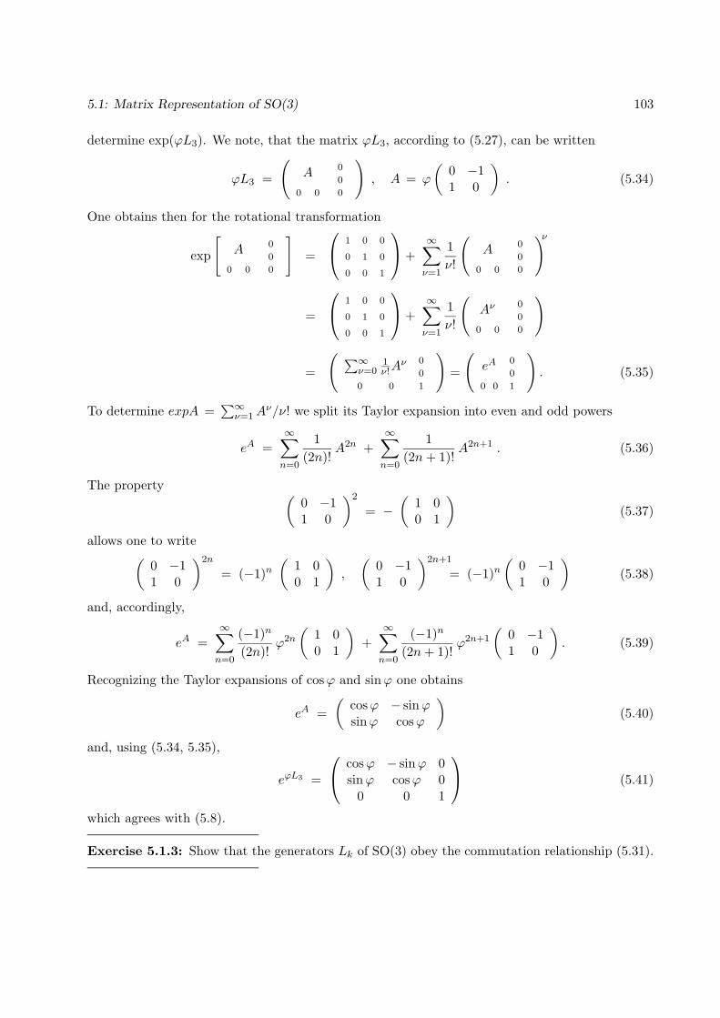
5.1: Matrix Representation of SO(3) 103
determine exp(ϕL3). We note, that the matrix ϕL3, according to (5.27), can be written
ϕL3 =
(A 0
0
0 0 0
), A = ϕ
(0 −11 0
). (5.34)
One obtains then for the rotational transformation
exp
[A 0
0
0 0 0
]=
1 0 0
0 1 0
0 0 1
+∞∑ν=1
1ν!
(A 0
0
0 0 0
)ν
=
1 0 0
0 1 0
0 0 1
+∞∑ν=1
1ν!
(Aν 0
0
0 0 0
)
=
( ∑∞ν=0
1ν!A
ν 0
0
0 0 1
)=
(eA 0
0
0 0 1
). (5.35)
To determine expA =∑∞
ν=1Aν/ν! we split its Taylor expansion into even and odd powers
eA =∞∑n=0
1(2n)!
A2n +∞∑n=0
1(2n+ 1)!
A2n+1 . (5.36)
The property (0 −11 0
)2
= −(
1 00 1
)(5.37)
allows one to write(0 −11 0
)2n
= (−1)n(
1 00 1
),
(0 −11 0
)2n+1
= (−1)n(
0 −11 0
)(5.38)
and, accordingly,
eA =∞∑n=0
(−1)n
(2n)!ϕ2n
(1 00 1
)+
∞∑n=0
(−1)n
(2n+ 1)!ϕ2n+1
(0 −11 0
). (5.39)
Recognizing the Taylor expansions of cosϕ and sinϕ one obtains
eA =(
cosϕ − sinϕsinϕ cosϕ
)(5.40)
and, using (5.34, 5.35),
eϕL3 =
cosϕ − sinϕ 0sinϕ cosϕ 0
0 0 1
(5.41)
which agrees with (5.8).
Exercise 5.1.3: Show that the generators Lk of SO(3) obey the commutation relationship (5.31).
104 Theory of Angular Momentum and Spin
5.2 Function space representation of the group SO(3)
In this section we will investigate how rotational transformations act on single particle wavefunctionsψ(~r). In particular, we will learn that transformation patterns and invariances are connected withthe angular momentum states of quantum mechanics.
Definition
We first define how a rotational transformation acts on a wavefunction ψ(~r ). For this purpose werequire stringent continuity properties of the wavefunction: the wavefunctions under considerationmust be elements of the set C∞(3), i.e., complex-valued functions over the 3-dimensional space R3which can be differentiated infinitely often. In analogy to R(~ϑ) being a linear map R3 → R3, wedefine rotations R(~ϑ) as linear maps C∞(3) → C∞(3), namely
R(~ϑ)ψ(~r ) = ψ(R−1(~ϑ)~r ) . (5.42)
Obviously, the transformation R(~ϑ): C∞(3) → C∞(3) is related to the transformation R(~ϑ):R3 → R3, a relationship which we like to express as follows
R(~ϑ) = ρ(R(~ϑ)
). (5.43)
ρ( ) conserves the group property of SO(3), i.e. for A, B ∈ SO(3) holds
ρ(AB) = ρ(A) ρ(B) . (5.44)
This important property which makes ρ( SO(3) ) also into a group can be proven by considering
ρ(R(~ϑ1)R(~ϑ2)
)ψ(~r) = ψ([R(~ϑ1)R(~ϑ2) ]−1~r) (5.45)
= ψ([R(~ϑ2)]−1 [R(~ϑ1)]−1~r ) = ρ(R(~ϑ2)
)ψ([R(~ϑ1)]−1~r) (5.46)
= ρ(R(~ϑ1)
)ρ(R(~ϑ2)
)ψ(~r) . (5.47)
Since this holds for any ψ(~r ) one can conclude ρ(R(~ϑ1)
)ρ(R(~ϑ2)
)= ρ
(R(~ϑ1)R(~ϑ2)
), i.e. the
group property (5.44) holds.
Exercise 5.2.1: Assume the definition ρ′(R(~ϑ)
)ψ(~r) = ψ(R(~ϑ)~r ). Show that in this case holds
ρ′(AB) = ρ′(B) ρ′(A).
Generators
One can assume then that R(~ϑ) should also form a Lie group, in fact, one isomorphic to SO(3)and, hence, its elements can be represented through an exponential
R(~ϑ) = exp(− i~
~ϑ · ~J)
(5.48)

5.2: Function Space Representation of SO(3) 105
where the generators can be determined in analogy to Eq. (5.22) according to
− i~
J1 = limϑ1→0
ϑ−11
(R(~ϑ = (−ϑ1, 0, 0)T ) − 1
)(5.49)
(note the minus sign of −ϑ1 which originates from the inverse of the rotation in Eq.(5.42)) andsimilarly for J2 and J3.The generators Jk can be determined by applying (5.49) to a function f(~r), i.e., in case of J3,
− i~
J3 f(~r) = limϑ3→0
ϑ−13
(R(~ϑ = (0, 0, ϑ3)T ) f(~r) − f(~r)
)= lim
ϑ3→0ϑ−1
3 ( f(R(0, 0,−ϑ3)~r ) − f(~r) ) . (5.50)
Using (5.23, 5.24) one can expand
R(0, 0,−ϑ3)~r ≈
1 ϑ3 0−ϑ3 1 0
0 0 1
x1
x2
x3
=
x1 + ϑ3x2
−ϑ3x1 + x2 .x3
(5.51)
Inserting this into (5.50) and Taylor expansion yields
− i~
J3 f(~r) = limϑ3→0
ϑ−13 ( f(~r) + ϑ3 x2 ∂1f(~r) − ϑ3 x1 ∂2f(~r) − f(~r) )
= (x2 ∂1 − x1 ∂2 ) f(~r) . (5.52)
Carrying out similar calculations for J1 and J2 one can derive
− i~
J1 = x3∂2 − x2∂3 (5.53)
− i~
J2 = x1∂3 − x3∂1 (5.54)
− i~
J3 = x2∂1 − x1∂2 . (5.55)
Not only is the group property of SO(3) conserved by ρ( ), but also the Lie algebra of the generators.In fact, it holds
[Jk, J`] = i ~ εk`m Jm . (5.56)
We like to verify this property for [J1, J2]. One obtains using (5.53–5.55) and f(~r) = f
[J1,J2] f(~r) = −~2 [− i~J1,− i
~J2] f(~r) = −~2×
[ (x3∂2 − x2∂3) (x1∂3f − x3∂1f) − (x1∂3 − x3∂1) (x3∂2f − x2∂3f) ]= −~2 [ +x1x3∂2∂3f − x1x2∂
23f − x2
3∂1∂2f + x2x3∂1∂3f + x2∂1f
−x1∂2f − x1x3∂2∂3f + x23∂1∂2f + x1x2∂
23f − x2x3∂1∂3f ]
= −~2 (x2∂1 − x1∂2 ) f(~r) = i~J3 f(~r) . (5.57)
Exercise 5.2.2: (a) Derive the generators Jk, k = 1, 2 by means of limits as suggested in Eq. (5.49);show that (5.56) holds for [J2, J3] and [J3, J1].

106 Theory of Angular Momentum and Spin
Exercise 5.2.3: Consider a wave function ψ(φ) which depends only on the azimutal angle φ of thespherical coordinate system (r, θ, φ), i.e. the system related to the Cartesian coordinates throughx1 = r sinθ cosφ, x2 = r sinθ sinφ, and x3 = r cosθ. Show that for J3 as defined above holdsexp( iα
~J3)ψ(φ) = ψ(φ + α).
5.3 Angular Momentum Operators
The generators Jk can be readily recognized as the angular momentum operators of quantummechanics. To show this we first note that (5.53–5.55) can be written as a vector product of ~r and∇
− i~
~J = −~r × ∇ . (5.58)
From this follows, using the momentum operator ~p = ~
i∇,
~J = ~r × ~
i∇ = ~r × ~p (5.59)
which, according to the correspondence principle between classical and quantum mechanics, iden-tifies ~J as the quantum mechanical angular momentum operator.Equation (5.56) are the famous commutation relationships of the quantium mechanical angularmomentum operators. The commutation relationships imply that no simultaneous eigenstates ofall three Jk exist. However, the operator
J 2 = J 21 + J 2
2 + J 23 (5.60)
commutes with all three Jk, k = 1, 2, 3, i.e.,
[J 2,Jk] = 0 , k = 1, 2, 3 . (5.61)
We demonstrate this property for k = 3. Using [AB,C] = A[B,C] + [A,C]B and (5.56) oneobtains
[J 2,J3] = [J 21 + J 2
2 ,J3] (5.62)= J1 [J1,J3] + [J1,J3]J1 + J2 [J2,J3] + [J2,J3]J2
= −i~J1 J2 − i~J2 J1 + i~J2 J1 + i~J1 J2 = 0
According to (5.61) simultaneous eigenstates of J 2 and of one of the Jk, usually chosen as J3, canbe found. These eigenstates are the well-known spherical harmonics Y`m(θ, φ). We will show nowthat the properties of spherical harmonics
J 2 Y`m(θ, φ) = ~2`(`+ 1)Y`m(θ, φ) (5.63)
J3 Y`m(θ, φ) = ~mY`m(θ, φ) (5.64)
as well as the effect of the so-called raising and lowering operators
J± = J1 ± iJ2 (5.65)
5.3: Angular Momentum Operators 107
on the spherical harmonics, namely,
J+ Y`m(θ, φ) = ~
√(`+m+ 1)(`−m)Y`m+1(θ, φ) (5.66)
J+ Y``(θ, φ) = 0 (5.67)J− Y`m+1(θ, φ) = ~
√(`+m+ 1)(`−m)Y`m(θ, φ) (5.68)
J− Y`−`(θ, φ) = 0 (5.69)
are a consequence of the Lie algebra (5.56). For this purpose we prove the following theorem.
An Important Theorem
Theorem 1.1 Let Lk, k = 1, 2, 3 be operators acting on a Hilbert space H which obey the algebra[Lk, L`] = εk`m Lm and let L± = L1 ± i L2, L2 = L2
1 + L22 + L2
3. Let there exist states |` `〉 inH with the property
L+ |` `〉 = 0 (5.70)L3 |` `〉 = −i ` |` `〉 (5.71)
then the states defined throughL− |`m+ 1〉 = −i βm |`m〉 (5.72)
have the following properties
(i) L+ |`m〉 = −i αm |`m+ 1〉 (5.73)(ii) L3 |`m〉 = −im |`m〉 (5.74)
(iii) L2 |`m〉 = − `(`+ 1) |`m〉 (5.75)
To prove this theorem we first show by induction that (i) holds. For this purpose we first demon-strate that the property holds for m = `− 1 by considering (i) for the state L−|``〉 ∼ |``− 1〉. Itholds L+L−|``〉 = (L+L− − L−L+ + L−L+)|` `〉 = ([L+, L−] + L−L+)|` `〉. Noting [L+, L−] =[L1 + iL2, L1 − iL2] = −2iL3 and L+|` `〉 = 0 one obtains L+L−|``〉 = −2iL3|``〉 = −2`|``〉,i.e., in fact, L+ raises the m-value of |`` − 1〉 from m = ` − 1 to m = `. The definitions of thecoefficients α`−1 and β`−1 yield L+L−|``〉 = L+( iβ`−1|``− 1〉 = −α`−1β`−1 |``〉, i.e.
α`−1β`−1 = 2` . (∗) (5.76)
We now show that property (ii) also holds for m = ` − 1 proceeding in a similar way. We noteL3L−|``〉 = ( [L3, L−] + L−L3 ) |``〉. Using [L3, L−] = [L3, L1 − iL2] = L2 + iL1 = i (L1 −iL2) = iL− and L3|``〉 = −i`|``〉 we obtain L3L−|``〉 = ( iL− + L−L3 )|``〉 = i(−` + 1)L−|``〉.From this follows that L−|``〉 is an eigenstate of L3, and since we have already shown |`` − 1〉 =(iβ`−1)−1L−|``〉 we can state L3|``− 1〉 = −i(`− 1)|``− 1〉.Continuing our proof through induction we assume now that property (i) holds for m. We willshow that this property holds then also for m − 1. The arguments are very similar to the onesused above and we can be brief. We consider L+L−|`m〉 = ( [L+, L−] + L−L+ )|`m〉 = (−2iL3 +
108 Theory of Angular Momentum and Spin
L−L+ )|`m〉 = (−2m − αmβm )|`m〉. This implies that (i) holds for m − 1, in particular, fromL+L−|`m〉 = −αm−1βm−1|`m〉 follows the recursion relationship
αm−1βm−1 = 2m + αmβm . (∗∗) (5.77)
We will show now that if (ii) holds for m, it also holds for m− 1. Again the argumemts are similarto the ones used above. We note L3L−|`m〉 = ( [L3, L−] + L−L3 )|`m〉 = ( iL− − imL− )|`m〉 =−i (m− 1)L−|`m〉 from which we can deduce L3|`m− 1〉 = −i(m− 1)|`m− 1〉.Before we can finally show that property (iii) holds as well for all −` ≤ m ≤ ` we need to determinethe coefficients αm and βm. We can deduce from (∗) and (∗∗)
α`−1β`−1 = 2`α`−2β`−2 = 2 (`− 1 + `)α`−3β`−3 = 2 (`− 2 + `− 1 + `)
··
Obviously, it holds αmβm = 2(∑`
k=m+1 k)
. Using the familiar formula∑n
k=0 k = n (n + 1)/2one obtains
αmβm = (`+ 1) ` − (m+ 1)m = (`+ 1) ` + m` − `m − (m+ 1)m= (` + m + 1)(` − m) (5.78)
One can normalize the states |`m〉 such that αm = βm, i.e., finally
αm = βm =√
(` + m + 1)(` − m) . (5.79)
We can now show that (iii) holds for all proper m–values. We note that we can write L2 =12L+L− + 1
2L−L+ + L23. It follows then L2|`m〉 = −
(12αm−1βm−1 + 1
2αmβm + m2)|`m〉 =
−(
12(`+m+ 1)(`−m)
+ 12(`+m)(`−m+ 1) + m2
)= − `(`+ 1)|`m〉. This completes the proof of the theorem.
We note that Eqs. (5.70, 5.72, 5.73, 5.79) read
L+|`m〉 = −i√
(`+m+ 1)(`−m) |`m+ 1〉 (5.80)L−|`m+ 1〉 = −i
√(`+m+ 1)(`−m) |`m〉 , (5.81)
i.e., yield properties (5.66, 5.69).We will have various opportunities to employ the Theorem just derived. A first application willinvolve the construction of the eigenstates of the angular momentum operators as defined in (5.63,5.64). For this purpose we need to express the angular momentum operators in terms of sphericalcoordinates (r, θ, φ.
Angular Momentum Operators in Spherical Coordinates
We want to express now the generators Jk, given in (5.53–5.55), in terms of spherical coordinatesdefined through
x1 = r sin θ cosφ (5.82)x2 = r sin θ sinφ (5.83)x3 = r cos θ (5.84)

5.3: Angular Momentum Operators 109
We first like to demonstrate that the generators Jk, actually, involve only the angular variables θand φ and not the radius r. In fact, we will prove
− i
~
J1 = L1 = sinφ∂
∂θ+ cot θ cosφ
∂
∂φ(5.85)
− i
~
J2 = L2 = − cosφ∂
∂θ+ cot θ sinφ
∂
∂φ(5.86)
− i
~
J3 = L3 = − ∂
∂φ. (5.87)
To derive these properties we consider, for example, L1f(θ, φ) = (x3∂2 − x2∂3)f(θ, φ). Using(5.82–5.84 ) one obtains, applying repeatedly the chain rule,
L1f(θ, φ) = (x3∂2 − x2∂3 ) f(θ, φ) (5.88)
=(x3∂x2/x1
∂x2
∂
∂ tanφ+ x3
∂x3/r
∂x2
∂
∂ cos θ(5.89)
− x2∂x2/x1
∂x3︸ ︷︷ ︸= 0
∂∂ tanφ − x2
∂x3/r∂x3
∂∂ cos θ
)f(θ, φ)
=(x3
x1
∂
∂ tanφ− x2
3x2
r3
∂
∂ cos θ− x2
x21 + x2
2
r3
∂
∂ cos θ
)f(θ, φ) (5.90)
This yields, using ∂/∂tanφ = cos2φ∂/∂φ and ∂/∂cosθ = −(1/sinθ) ∂/∂θ,
L1f(θ, φ) =(
cos θsin θ cosφ
cos2 φ∂
∂φ+ (5.91)
+cos2 θ sin θ sinφ
sin θ∂
∂θ+
sin θ sinφsin θ
sin2 θ∂
∂θ
)f(θ, φ)
which agrees with expression (5.85).We like to express now the operators J3 and J 2, the latter defined in (5.60), in terms of sphericalcoordinates. According to (5.87) holds
J3 =~
i∂φ . (5.92)
To determine J 2 we note, using (5.85),
(L1)2 =(
sinφ∂
∂θ+ cot θ cosφ
∂
∂φ
)2
= sin2φ∂2
∂θ2− 1
sin2θsinφ cosφ
∂
∂φ+ 2 cotθ sinφ cosφ
∂2
∂θ∂φ
+ cotθ cos2φ∂
∂θ+ cot2θ cos2φ
∂2
∂φ2(5.93)
and similarly, using (5.86),
(L2)2 =(− cosφ
∂
∂θ+ cot θ sinφ
∂
∂φ
)2

110 Theory of Angular Momentum and Spin
= cos2φ∂2
∂θ2+
1sin2θ
sinφ cosφ∂
∂φ− 2 cotθ sinφ cosφ
∂2
∂θ∂φ
+ cotθ sin2φ∂
∂θ+ cot2θ sin2φ
∂2
∂φ2. (5.94)
It follows
(L1)2 + (L2)2 + (L3)2 =∂2
∂θ2+ cotθ
∂
∂θ+ ( cot2θ + 1 )
∂2
∂φ2. (5.95)
With cot2θ + 1 = 1/sin2θ,
1sin2θ
(sinθ
∂
∂θ
) (sinθ
∂
∂θ
)=
∂2
∂θ2+ cotθ
∂
∂θ, (5.96)
and the relationship between Lk and Jk as given in (5.85, 5.86, 5.87), one can conclude
J 2 = − ~2
sin2θ
[(sinθ
∂
∂θ
)2
+∂2
∂φ2
]. (5.97)
Kinetic Energy Operator The kinetic energy of a classical particle can be expressed
~p 2
2m=
p2r
2m+
J2class
2mr2(5.98)
where ~Jclass = ~r × m~v is the angular momentum and pr = mr is the radial momentum. Thecorresponding expression for the quantum mechanical kinetic energy operator is
T = − ~2
2m∇2 = − ~
2
2m1r
∂2
∂r2r +
J 2
2mr2, (5.99)
which follows from the identity
∇2 =∂2
∂r2+
2r
∂
∂r+
1r2sin2θ
[(sinθ
∂
∂θ
)2
+∂2
∂φ2
](5.100)
1r
∂2
∂r2r =
∂2
∂r2+
2r
∂
∂r(5.101)
and comparision with (5.97).
5.4 Angular Momentum Eigenstates
According to the theorem on page 107 above the eigenfunctions (5.63, 5.64) can be constructed asfollows. One first identifies the Hilbert space H on which the generators Lk operate. The operatorsin the present case are Lk = − i
~Jk where the Jk are differential operators in θ and φ given in (5.85,
5.86, 5.87). These generators act on a subspace of C∞(3), namely on the space of complex-valuedfunctions on the unit 3-dim. sphere S2, i.e. C∞(S2). The functions in C∞(S2) have real variables

5.4: Angular Momentum Eigenstates 111
θ, φ, 0 ≤ θ < π, 0 ≤ φ < 2π, and to be admissable for description of quantum states, must becyclic in φ with period 2π. The norm in H is defined through
|f |2 =∫S2
dΩ f∗(θ, φ)f(θ, φ) (5.102)
where dΩ = sinθ dθ dφ is the volume element of S2. The function space endowed with this normand including only functions for which the integral (5.102) exists, is indeed a Hilbert space.The eigenfunctions (5.63, 5.64) can be constructed then by seeking first functions Y``(θ, φ) in Hwhich satisfy L+Y``(θ, φ) = 0 as well as L3Y``(θ, φ) = −i` Y``(θ, φ), normalizing these functions,and then determining the family Y`m(θ, φ),m = −`,−`+ 1, . . . , ` applying
L−Y`m+1(θ, φ) = −i√
(`+m+ 1)(`−m)Y`m(θ, φ) (5.103)
iteratively for m = `− 1, `− 2, . . . ,−`. One obtains in this way
Y`m(θ, φ) = ∆(`,m)(
1~
J−)`−m
Y``(θ, φ) (5.104)
∆(`,m) =[
(` + m)!(2`)! (` − m)!
] 12
(5.105)
Constructing Y`` → Y``−1 →→ · · · Y`−`
We like to characterize the resulting eigenfunctions Y`m(θ, φ), the so-called spherical harmonics, bycarrying out the construction according to (5.104, 5.105) explicitly. For this purpose we split offa suitable normalization factor as well as introduce the assumption that the dependence on φ isdescribed by a factor exp(imφ)
Y`m(θ, φ) =
√2`+ 1
4π(`−m)!(`+m)!
P`m(cosθ) eimφ . (5.106)
It must hold
L+ Y``(θ, φ) = 0 (5.107)L3 Y``(θ, φ) = −i ` Y``(θ, φ) . (5.108)
The latter property is obviously satisfied for the chosen φ-dependence. The raising and loweringoperators
L± = L1 ± iL2 , (5.109)
using (5.85–5.87), can be expressed
L± = ∓ i e±iφ(∂
∂θ± i cotθ
∂
∂φ
). (5.110)
Accordingly, (5.107) reads (∂
∂θ+ i cotθ
∂
∂φ
)P``(cosθ) ei`φ = 0 (5.111)
112 Theory of Angular Momentum and Spin
or (∂
∂θ− ` cotθ
)P``(cosθ) = 0 (5.112)
where we employed the definition of P``(cosθ) in (5.107). A proper solution of this equation, i.e.,one for which ∫ π
0dθ sinθ |P``(cosθ)|2 (5.113)
is finite, isP``(cos θ) = N` sin` θ (5.114)
as one can readily verify. The normalization factor N` is chosen such that∫ π
0dθ sinθ |Y``(cosθ)|2 = 1 (5.115)
holds. (5.106, 5.114) yield
|N`|22`+ 1
4π1
(2`)!2π∫ π
0dθ sin2`+1θ = 1 . (5.116)
The integral appearing in the last expression can be evaluated by repeated integration by parts.One obtains, using the new integration variable x = cos θ,∫ π
0dθ sin2`+1θ =
∫ +1
−1dx (1 − x2)`
=[x (1 − x2)`
]+1
−1+ 2`
∫ +1
−1dxx2 (1 − x2)`−1
= 2`[x3
3(1 − x2)`−1
]+1
−1
+2` · (2`− 2)
1 · 3
∫ +1
−1dxx4 (1 − x2)`−2
...
=2` · (2`− 2) · · · 2
1 · 3 · 5 · · · (2`− 1)
∫ +1
−1dxx2`
=2` · (2`− 2) · · · 2
1 · 3 · 5 · · · (2`− 1)2
2`+ 1=
(2`)![1 · 3 · 5 · · · (2`− 1)]2
22`+ 1
(5.117)
Accordingly, (5.116) implies
|N`|21
[1 · 3 · 5 · · · (2`− 1)]2= 1 (5.118)
from which we concludeN` = (−1)` 1 · 3 · 5 · · · (2`− 1) (5.119)
where the factor (−1)` has been included to agree with convention1. We note that (5.106, 5.114,5.119) provide the following expression for Y``
Y``(θ, φ) = (−1)`√
2`+ 14π
1(2`)!
12``!
sin` θ ei`φ . (5.120)
1See, for example, ”Classical Electrodynamics, 2nd Ed.” by J.D. Jackson (John Wiley, New York, 1975)
5.4: Angular Momentum Eigenstates 113
We have constructed a normalized solution of (5.106), namely Y``(θ, φ), and can obtain now, throughrepeated application of (5.103, 5.110), the eigenfunctions Y`m(θ, φ), m = `−1, `−2, . . .−` definedin (5.63, 5.64). Actually, we seek to determine the functions P`m(cos θ) and, therefore, use (5.103,5.110) together with (5.106)
i e−iφ(∂
∂θ− i cotθ
∂
∂φ
) √2`+ 1
4π(`−m− 1)!(`+m+ 1)!
P`m+1(cos θ) ei(m+1)φ
= −i√
(`+m+ 1)(`−m)
√2`+ 1
4π(`−m)!(`+m)!
P`m(cos θ) eimφ. (5.121)
This expressions shows that the factor eimφ, indeed, describes the φ-dependence of Y`m(θ, φ); everyapplication of L− reduces the power of eiφ by one. (5.121) states then for the functions P`m(cos θ)(
∂
∂θ+ (m+ 1) cotθ
)P`m+1(cos θ) = − (`+m+ 1) (`−m)P`m(cos θ) . (5.122)
The latter identity can be written, employing again the variable x = cos θ,
P`m(x) =−1
(`+m+ 1) (`−m)× (5.123)
×
[−(1− x2)
12∂
∂x+ (m+ 1)
x
(1− x2)12
]P`m+1(x) .
We want to demonstrate now that the recursion equation (5.123) leads to the expression
P`m(x) =1
2``!(`+m)!(`−m)!
(1− x2)−m2∂`−m
∂x`−m(x2 − 1)` (5.124)
called the associated Legendre polynomials. The reader should note that the associated Legendrepolynomials, as specified in (5.124), are real. To prove (5.124) we proceed by induction. For m = `(5.124) reads
P``(x) =(2`)!2``!
(1− x2)−`2 (x2 − 1)`
= (−1)` 1 · 3 · 5 · · · (2`− 1) sin` θ (5.125)
which agrees with (5.114, 5.119). Let us then assume that (5.124) holds for m+ 1, i.e.,
P`m+1(x) =1
2``!(`+m+ 1)!(`−m− 1)!
(1− x2)−m+1
2∂`−m−1
∂x`−m−1(x2 − 1)` . (5.126)
Then holds, according to (5.123),
P`m(x) =−12``!
(`+m)!(`−m)!
[−(1− x2)
12∂
∂x+ (m+ 1)
x
(1− x2)12
]×
× (1− x2)−m+1
2∂`−m−1
∂x`−m−1(x2 − 1)` . (5.127)
114 Theory of Angular Momentum and Spin
By means of
−(1− x2)12∂
∂x(1− x2)−
m+12
∂`−m−1
∂x`−m−1(x2 − 1)`
= −(1− x2)−m2∂`−m
∂x`−m(x2 − 1)`
− (m+ 1)x
(1− x2)12
(1− x2)−m+1
2∂`−m−1
∂x`−m−1(5.128)
one can show that (5.127) reproduces (5.124) and, therefore, that expression (5.124) holds for m ifit holds for m+ 1. Since (5.124) holds for m = `, it holds then for all m.We want to test if the recursion (5.123) terminates for m = −`, i.e., if
L− Y``(θ, φ) = 0 (5.129)
holds. In fact, expression (5.124), which is equivalent to recursive application of L−, yields avanishing expression for m = −`− 1 as long as ` is a non-negative integer. In that case (1− x2)`
is a polynomial of degree 2` and, hence, the derivative ∂2`+1/∂x2`+1 of this expression vanishes.
Constructing Y`−` → Y`−`+1 → · · ·Y``
An alternative route to construct the eigenfunctions Y`m(θ, φ) determines first a normalized solutionof
L− f(θ, φ) = 0 (5.130)L3 f(θ, φ) = i ` f(θ, φ) , (5.131)
identifies f(θ, φ) = Y`−`(θ, φ) choosing the proper sign, and constructs then the eigenfunctionsY`−`+1, Y`−`+2, etc. by repeated application of the operator L+. Such construction reproducesthe eigenfunctions Y`m(θ, φ) as given in (5.106, 5.124) and, therefore, appears not very interesting.However, from such construction emerges an important symmetry property of Y`m(θ, φ), namely,
Y ∗`m(θ, φ) = (−1)m Y`−m(θ, φ) (5.132)
which reduces the number of spherical harmonics which need to be evaluated independently roughlyby half ; therefore, we embark on this construction in order to prove (5.132).We first determine Y`−`(θ, φ) using (5.106, 5.124). It holds, using x = cos θ,
P`−`(x) =1
2``!1
(2`)!(1− x2)
`2∂2`
∂x2`(x2 − 1)` . (5.133)
Since the term with the highest power of (x2 − 1)` is x2`, it holds
∂2`
∂x2`(x2 − 1)` = (2`)! (5.134)
and, therefore,
P`−`(x) =1
2``!(1− x2)
`2 . (5.135)

5.4: Angular Momentum Eigenstates 115
Due to (5.106, 5.124) one arrives at
Y`−`(θ, φ) =
√2`+ 1
4π1
(2`)!1
2``!sin` θ e−i`φ . (5.136)
We note in passing that this expression and the expression (5.120) for Y`` obey the postulatedrelationship (5.132).Obviously, the expression (5.136) is normalized and has the proper sign, i.e., a sign consistent withthe family of functions Y`m constructed above. One can readily verify that this expression providesa solution of (5.129). This follows from the identity(
∂
∂θ− i cotθ
∂
∂φ
)sin` θ e−i`φ = 0 . (5.137)
One can use (5.136) to construct all other Y`m(θ, φ). According to (5.80) and (5.110) applies therecursion
eiφ(∂
∂θ+ i cotθ
∂
∂φ
)Y`m(θ, φ) =
√(`+m+ 1)(`−m)Y`m+1(θ, φ) . (5.138)
Employing (5.106), one can conclude for the associated Legendre polynomials√(`−m)!(`+m)!
(∂
∂θ− m cotθ
)P`m(cos θ)
=√
(`+m+ 1)(`−m)
√(`−m− 1)!(`+m+ 1)!
P`m+1(cos θ) (5.139)
or
P`m+1(cos θ) =(∂
∂θ− m cotθ
)P`m(cos θ) . (5.140)
Introducing again the variable x = cos θ leads to the recursion equation [c.f. (5.122, 5.123)]
P`m+1(x) =
(−(1− x2)
12∂
∂x− m
x
(1− x2)12
)P`m(x) . (5.141)
We want to demonstrate now that this recursion equation leads to the expression
P`m(x) =(−1)m
2``!(1− x2)
m2∂`+m
∂x`+m(x2 − 1)` (5.142)
For this purpose we proceed by induction, following closely the proof of eq. (5.124). We first notethat for m = −` (5.142) yields
P`−`(x) =(−1)`
2``!(1− x2)−
`2 (x2 − 1)` =
12``!
(1− x2)`2 (5.143)
116 Theory of Angular Momentum and Spin
wich agrees with (5.135). We then assume that (5.142) holds for m. (5.141) reads then
P`m+1(x) = (5.144)(−(1− x2)
12∂
∂x− m
x
(1− x2)12
)(−1)m
2``!(1− x2)
m2∂`+m
∂x`+m(x2 − 1)` .
Replacing in (5.128) m+ 1 → −m or, equivalently, m → −m− 1 yields
−(1− x2)12∂
∂x(1− x2)
m2∂`+m
∂x`+m(x2 − 1)`
= −(1− x2)m+1
2∂`+m+1
∂x`+m+1(x2 − 1)`
+ mx
(1− x2)12
(1− x2)m2∂`+m
∂x`+m. (5.145)
Hence, (5.144) reads
P`m+1(x) =(−1)m+1
2``!(1− x2)
m+12
∂`+m+1
∂x`+m+1(x2 − 1)` , (5.146)
i.e., (5.142) holds for m + 1 if it holds for m. Since (5.142) holds for m = −` we verified that itholds for all m.The construction beginning with Y`−` and continuing with Y`−`+1, Y`−`+2, etc. yields the sameeigenfunctions as the previous construction beginning with Y`` and stepping down the series offunctions Y``−1, Y``−2, etc. Accordingly, also the associated Legendre polynomials determined thisway, i.e., given by (5.142) and by (5.124), are identical. However, one notes that application of(5.124) yields
(−1)m(`−m)!(`+m)!
P`−m(x) =(−1)m
2``!(1− x2)
m2∂`+m
∂x`+m(x2 − 1)` , (5.147)
the r.h.s. of which agrees with the r.h.s. of (5.142). Hence, one can conclude
P`m(x) = (−1)m(`−m)!(`+m)!
P`−m(x) . (5.148)
According to (5.106) this implies for Y`m(θ, φ) the identity (5.132).
The Legendre Polynomials
The functionsP`(x) = P`0(x) (5.149)
are called Legendre polynomials. According to both (5.124) and (5.142) one can state
P`(x) =1
2``!∂`
∂x`(x2 − 1)` . (5.150)
5.4: Angular Momentum Eigenstates 117
The first few polynomials are
P0(x) = 1 , P1(x) = x , P2(x) = 12(3x2 − 1)
P3(x) = 12 (5x3 − 3x) . (5.151)
Comparision of (5.150) and (5.142) allows one to express the associated Legendre polynomials interms of Legendre polynomials
P`m(x) = (−1)m (1− x2)m2∂m
∂xmP`(x) , m ≥ 0 (5.152)
and, accordingly, the spherical harmonics for m ≥ 0
Y`m(θ, φ) =
√2`+ 1
4π(`−m)!(`+m)!
(−1)m sinm θ × (5.153)
×(
∂
∂ cos θ
)mP`(cos θ) eimφ .
The spherical harmonics for m < 0 can be obtained using (5.132).The Legendre polynomials arise in classical electrodynamics as the expansion coefficients of theelectrostatic potential around a point charge q/|~r1 − ~r2| where q is the charge, ~r1 is the point wherethe potential is measured, and ~r2 denotes the location of the charge. In case q = 1 and |~r2| < |~r1|holds the identity2
1|~r1 − ~r2|
=∞∑`=0
r`2r`+1
1
P`(cos γ) (5.154)
where γ is the angle between ~r1 and ~r2. Using x = cos γ, t = r2/r1, and
|~r1 − ~r2| = r1
√1 − 2x t + t2 , (5.155)
(5.154) can be written
w(x, t) =1√
1 − 2xt + t2=
∞∑`=0
P`(x) t` . (5.156)
w(x, t) is called a generating function of the Legendre polynomials3.The generating function allows one to derive useful properties of the Legendre polynomials. Forexample, in case of x = 1 holds
w(1, t) =1√
1 − 2t + t2=
11 − t
=∞∑`=0
t` . (5.157)
Comparision with (5.156) yields
P`(1) = 1 , ` = 0, 1, 2, . . . (5.158)2see, e.g., ”Classical Electrodynamics, 2nd Ed.” by J.D. Jackson (John Wiley, New York, 1975), pp. 923To prove this property see, for example, pp. 45 of “Special Functions and their Applications” by N.N. Lebedev
(Prentice-Hall, Englewood Cliffs, N.J., 1965) which is an excellent compendium on special functions employed inphysics.

118 Theory of Angular Momentum and Spin
For w(x, t) holds∂lnw(x, t)
∂t=
x − t
1 − 2xt + t2. (5.159)
Using ∂lnw/∂t = (1/w) ∂w/∂t and multiplying (5.159) by w(1 − 2xt + t2) leads to the differentialequation obeyed by w(x, t)
(1 − 2xt + t2)∂w
∂t+ (t − x)w = 0 . (5.160)
Employing (5.156) and (∂/∂t)∑
` P`(x)t` =∑
` `P`(x)t`−1 this differential equation is equivalentto
(1 − 2xt + t2)∞∑`=0
`P`(x) t`−1 + (t − x)∞∑`=0
P`(x) t` = 0 (5.161)
Collecting coefficients with equal powers t` yields
0 = P1(x) − xP0(x) (5.162)
+∞∑`=1
[(`+ 1)P`+1(x) − (2`+ 1)xP`(x) + ` P`−1(x) ] t`
The coefficients for all powers t` must vanish individually. Accordingly, holds
P1(x) = xP0(x) (5.163)(` + 1)P`+1(x) = (2` + 1)xP`(x) − ` P`−1(x) (5.164)
which, using P0(x) = 1 [c.f. (5.151)] allows one to determine P`(x) for ` = 1, 2, . . ..
Inversion Symmetry of Y`m(θ, φ) Under inversion at the origin vectors ~r are replaced by −~r.If the spherical coordinates of ~r are (r, θ, φ), then the coordinates of −~r are (r, π − θ, π + φ).Accordingly, under inversion Y`m(θ, φ) goes over to Y`m(π− θ, π+ φ). Due to cos(π− θ) = − cos θthe replacement ~r → −~r alters P`m(x) into P`m(−x). Inspection of (5.142) allows one to conclude
P`m(−x) = (−1)`+m P`m(x) (5.165)
since ∂n/∂(−x)n = (−1)n∂n/∂xn. Noting exp[im(π + φ)] = (−1)mexp(imφ) we determine
Y`m(π − θ, π + φ) = (−1)` Y`m(θ, φ) . (5.166)
Properties of Y`m(θ, φ)
We want to summarize the properties of the spherical harmonics Y`m(θ, φ) derived above.
1. The spherical harmonics are eigenfunctions of the angular momentum operators
J 2 Y`m(θ, φ) = ~2 `(`+ 1)Y`m(θ, φ) (5.167)
J3 Y`m(θ, φ) = ~mY`m(θ, φ) . (5.168)

5.4: Angular Momentum Eigenstates 119
2. The spherical harmonics form an orthonormal basis of the space C∞(S2) of normalizable,uniquely defined functions over the unit sphere S2 which are infinitely often differentiable∫ π
0sin θdθ
∫ 2π
0dφY ∗`′m′(θ, φ)Y`m(θ, φ) = δ`′`δm′m . (5.169)
3. The spherical harmonics form, in fact, a complete basis of C∞(S2), i.e., for any f(θ, φ) ∈C∞(S2) holds
f(θ, φ) =∞∑`=0
∑m=−`
C`m Y`m(θ, φ) (5.170)
C`m =∫ π
0sin θdθ
∫ 2π
0dφY ∗`m(θ, φ)f(θ, φ) . (5.171)
4. The spherical harmonics obey the recursion relationships
J+ Y`m(θ, φ) = ~
√(`+m+ 1)(`−m) Y`m+1(θ, φ) (5.172)
J− Y`m+1(θ, φ) = ~
√(`+m+ 1)(`−m) Y`m(θ, φ) (5.173)
where J± = J1 ± iJ2.
5. The spherical harmonics are given by the formula
Y`m(θ, φ) =
√2`+ 1
4π(`−m)!(`+m)!
(−1)m
2``!sinm θ × (5.174)
×(
∂
∂ cos θ
)mP`(cos θ) eimφ , m ≥ 0
where (` = 1, 2, . . .)
P0(x) = 1 , P1(x) = x , (5.175)P`+1(x) = 1
`+ 1 [ (2` + 1)xP`(x) − ` P`−1(x) ] (5.176)
are the Legendre polynomials. The spherical harmonics for m < 0 are given by
Y`−m(θ, φ) = (−1)m Y ∗`m(θ, φ) . (5.177)
Note that the spherical harmonics are real, except for the factor exp(imφ).
6. The spherical harmonics Y`0 are
Y`0(θ, φ) =
√2`+ 1
4πP`(cos θ) . (5.178)
7. For the Legendre polynomials holds the orthogonality property∫ +1
−1dx P`(x)P (`′(x) =
22` + 1
δ``′ . (5.179)
120 Theory of Angular Momentum and Spin
8. The spherical harmonics for θ = 0 are
Y`m(θ = 0, φ) = δm0
√2`+ 1
4π. (5.180)
9. The spherical harmonics obey the inversion symmetry
Y`m(θ, φ) = (−1)` Y`m(π − θ, π + φ) . (5.181)
10. The spherical harmonics for ` = 0, 1, 2 are given by
Y00 =1√4π
(5.182)
Y11 = −√
38π
sin θ eiφ (5.183)
Y10 =
√3
4πcos θ (5.184)
Y22 =14
√152π
sin2 θ e2iφ (5.185)
Y21 = −√
158π
sin θ cos θ eiφ (5.186)
Y20 =
√5
4π
(32
cos2 θ − 12
)(5.187)
together with (5.177).
11. For the Laplacian holds
∇2 h(r)Y`m(θ, φ) =[
1r
∂2
∂r2r − `(`+ 1)
r2
]h(r)Y`m(θ, φ) . (5.188)
Exercise 5.4.1: Derive expressions (5.86), (5.87).Exercise 5.4.2: Derive the orthogonality property for the Legendre polynomials (5.179) using thegenerating function w(x, t) stated in (5.156). For this purpose start from the identity∫ +1
−1dx w(x, t)2 =
∞∑`,`′=0
t`+`′∫ +1
−1dxP`(x)P`′(x) , (5.189)
evaluate the integral on the l.h.s., expand the result in powers of t and equate the resulting powersto those arising on the r.h.s. of (5.189).Exercise 5.4.3: Construct all spherical harmonics Y3m(θ, φ).

5.5: Irreducible Representations 121
5.5 Irreducible Representations
We will consider now the effect of the rotational transformations introduced in (5.42),exp
(− i~
~ϑ · ~J)
, on functions f(θ, φ) ∈ C∞(S2). We denote the image of a function f(θ, φ)
under such rotational transformation by f(θ, φ), i.e.,
f(θ, φ) = exp(− i~
~ϑ · ~J)f(θ, φ) . (5.190)
Since the spherical harmonics Y`m(θ, φ) provide a complete, orthonormal basis for the functionspace C∞(S2) one can expand
f(θ, φ) =∑`,m
c`m Y`m(θ, φ) (5.191)
c`m =∫S2
dΩ′ Y ∗`m(θ′, φ′) exp(− i~
~ϑ · ~J)f(θ′, φ′) (5.192)
One can also represent C∞(S2)
C∞(S2) = [ Y`m, ` = 0,1, . . . ∞, m = −`,−`+ 1, . . . , ` ] (5.193)
where [ ] denotes closure of a set by taking all possible linear combinations of the elementsof the set. The transformations exp
(− i~
~ϑ · ~J)
, therefore, are characterized completely if onespecifies the transformation of any Y`m(θ, φ)
Y`m(θ, φ) =∑`′,m′
[D(~ϑ)
]`′m′; `m
Y`m(θ, φ) (5.194)
[D(~ϑ)
]`′m′; `m
=∫S2
dΩY ∗`′m′(θ, φ) exp(− i~
~ϑ · ~J)Y`m(θ, φ) , (5.195)
i.e., if one specifies the functional form of the coefficients [D(ϑ)]`′m′; `m. These coefficients canbe considered the elements of an infinite-dimensional matrix which provides the representation ofexp
(− i~
~ϑ · ~J)
in the basis Y`m, ` = 0, 1, . . . ∞, m = −`,−`+ 1, . . . , `.We like to argue that the matrix representing the rotational transformations of the function spaceC∞(S2), with elements given by (5.195), assumes a particularly simple form, called the irreduciblerepresentation. For this purpose we consider the subspaces of C∞(S2)
X` = [ Y`m, m = −`,−`+ 1, . . . , ` ] , ` = 0,1,2, . . . (5.196)
Comparision with (5.193) shows
C∞(S2) =∞⋃`=1
X` . (5.197)
The subspaces X` have the important property that (i) they are invariant under rotationsexp
(− i~
~ϑ · ~J)
, i.e., exp(− i~
~ϑ · ~J)
(X`) = X`, and (ii) they form the lowest dimensional sets X`obeying C∞(S2) =
⋃` X` which have this invariance property.
122 Theory of Angular Momentum and Spin
The invariance of the subspaces X` under rotations follows from a Taylor expansion of the expo-nential operator exp
(− i~
~ϑ · ~J)
. One proceeds by expanding first ~ϑ · ~J in terms of J+, J−, andJ3
ϑ · ~J =12ϑ−J+ +
12ϑ+J− + ϑ3J3 (5.198)
where ϑ± = ϑ1 ∓ ϑ2. The exponential operator exp(− i~
~ϑ · ~J)
can be expanded in powers
(12ϑ−J+ + 1
2ϑ+J− + ϑ3J3)n. One employs then the commutation properties
[J+, J−] = 2~J3 , [J3, J±] = ±~J± (5.199)
which follow readily from (5.56, 5.65). Application of (5.199) allows one to express
exp(− i~
~ϑ · ~J)
=∑
n1,n2,n3
cn1,n2,n3 Jn1+ J
n2− J
n33 . (5.200)
Accordingly, one needs to consider the action of J n1+ J
n2− J
n33 on the subspaces X`. Since the Y`m are
eigenfunctions of J3 the action of J n33 reproduces the basis functions of X`, i.e., leaves X` invariant.
The action of J− on Y`m produces Y`m−1 or, in case m = −`, produces 0, i.e., J n2− also leaves
X` invariant. Similarly, one can conclude that J n1+ leaves X` invariant. Since any additive term
in (5.200) leaves X` invariant, the transformation exp(− i~
~ϑ · ~J)
leaves X` invariant as well. Onecan conclude then that in the expansion (5.194) only spherical harmonics with `′ = ` contributeor, equivalently, one concludes for the matrix elements (5.195)
[D(ϑ)]`′m′; `m = δ`′`
∫S2
dΩY ∗`m′(θ, φ) exp(− i~
~ϑ · ~J)Y`m(θ, φ) . (5.201)
From expression (5.200) of the rotational transformations one can also conclude that the X` arethe smallest invariant subspaces of C∞(S2).If one orders the basis according to the partitoning (5.197) of C∞(S2) the matrix representation ofD(ϑ) assumes a block-diagonal form, with blocks of dimension 1, 3, 5, . . ., i.e.,
D(ϑ) =
1× 1
3× 3
. . .
(2`+ 1)× (2`+ 1)
. . .
(5.202)

5.6: Wigner Rotation Matrices 123
This representation of D(ϑ) is the one wich has blocks of the lowest dimensions possible. Therepresentation is referred to as the irreducible representation, other representations are termedreducible representations.
Exercise 5.5.1: Representations of the group SO(2)SO(2) is the set of all 2×2 matrices R which are orthogonal, i.e. for which holds RTR = RRT = 11,and for which detR = 1.(a) Show that SO(2) with the group operation defined as matrix multiplication, is a group.(b) Prove that the elements of SO(2) can be completely characterized through a single parameter.(c) Show that the map R(ϕ)(
xy
)=(x′
y′
)=(
cosϕ −sinϕsinϕ cosϕ
) (xy
)= R(ϕ)
(xy
)defines a representation of SO(2).(d) Show that the similarity transformation T (ϕ) defined in the space of non-singular, real 2× 2–matrices O through
O′ = T (ϕ)O = R(ϕ)OR−1(ϕ)
with R(ϕ) as in (c) is also a representation of SO(2).(e) In the space C∞(1) of infinitely often differentiable, and periodic functions f(α), i.e. f(α +2π) = f(α), the map ρ(ϕ) defined through
f(α)ρ→ g(ϕ) = f(α − ϕ) = ρ(ϕ)f(α)
also defines a representation of SO(2). Determine the generator of ρ(ϕ) in analogy to (5.22, 5.49).(f) The transformation ρ(ϕ) as defined in (e) leaves the following subspace of functions consideredin (e)
Xm = f(α) = Ae−imα, A ∈ C,m ∈ N
invariant. Give the corresponding expression of ρ(ϕ).
5.6 Wigner Rotation Matrices
We will now take an important first step to determine the functional form of the matrix elementsof D(ϑ). This step reconsiders the parametrization of rotations by the vector ~ϑ assumed sofar. Thethree components ϑk, k = 1, 2, 3 certainly allow one to describe any rotation around the origin.However, this parametrization, though seemingly natural, does not provide the simplest mathe-matical description of rotations. A more suitable parametrization had been suggested by Euler:every rotation exp
(− i~
~ϑ · ~J)
can be represented also uniquely by three consecutive rotations:
(i) a first rotation around the original x3–axis by an angle α,
(ii) a second rotation around the new x′2–axis by an angle β,
(iii) a third rotation around the new x′′3–axis by an angle γ.

124 Theory of Angular Momentum and Spin
The angles α, β, γ will be referred to as Euler angles. The axis x′2 is defined in the coordinate framewhich is related to the original frame by rotation (i), the axis x′′3 is defined in the coordinate framewhich is related to the original frame by the consecutive rotations (i) and (ii).The Euler rotation replaces exp
(− i~
~ϑ · ~J)
by
e−i~γJ ′′3 e−
i~βJ ′2 e−
i~αJ3 . (5.203)
For any ϑ ∈ R3 one can find Euler angles α, β, γ ∈ R such that
exp(− i~
~ϑ · ~J)
= e−i~γJ ′′3 e−
i~βJ ′2 e−
i~αJ3 (5.204)
is satisfied. Accordingly, one can replace (5.194, 5.195) by
Y`m(θ, φ) =∑`′,m′
[D(α, β, γ)]`′m′; `m Y`m(θ, φ) (5.205)
[D(α, β, γ)]`′m′; `m =∫S2
dΩY ∗`′m′(θ, φ) e−i~γJ ′′3 e−
i~βJ ′2 e−
i~αJ3Y`m(θ, φ) ,
(5.206)
The expression (5.203) has the disadvantage that it employs rotations defined with respect to threedifferent frames of reference. We will demonstrate that (5.203) can be expressed, however, in termsof rotations defined with respect to the original frame. For this purpose we notice that J ′2 can beexpressed through the similarity transformation
J ′2 = e−i~αJ3J2 e
i~αJ3 (5.207)
which replaces J ′2 by the inverse transformation (i), i.e., the transformation from the rotated frameto the original frame, followed by J2 in the original frame, followed by transformation (i), i.e., thetransformation from the original frame to the rotated frame. Obviously, the l.h.s. and the r.h.s. of(5.207) are equivalent. For any similarity transformation involving operators A and S holds
eS AS−1
= S eA S−1 . (5.208)
Accordingly, we can writee−
i~βJ ′2 = e−
i~αJ3 e−
i~βJ2 e
i~αJ3 (5.209)
The first two rotations in (5.203), i.e., (i) and (ii), can then be written
e−i~βJ ′2 e−
i~αJ3 = e−
i~αJ3 e−
i~βJ2 (5.210)
The third rotation in (5.203), in analogy to (5.209), is
e−i~γJ ′′3 = e−
i~βJ ′2 e−
i~αJ3 e−
i~γJ3 e
i~αJ3 e
i~βJ ′2 (5.211)
Using (5.209) in this expression one obtains
e−i~γJ ′′3 = e−
i~αJ3 e−
i~βJ2 e
i~αJ3 e−
i~αJ3 e−
i~γJ3 e
i~αJ3 e−
i~αJ3 e
i~βJ2 e
i~αJ3
= e−i~γJ ′′3 = e−
i~αJ3 e−
i~βJ2 e−
i~γJ3 e
i~βJ2 e
i~αJ3 (5.212)
5.7: Spin 12 and the group SU(2) 125
Multiplication from the left with (5.210) yields the simple result
e−i~γJ ′′3 e−
i~βJ ′2 e−
i~αJ3 = e−
i~αJ3 e−
i~βJ2 e−
i~γJ3 , (5.213)
i.e., to redefine the three rotations in (5.203) with respect to the original (unprimed) frame onesimply needs to reverse the order of the rotations. This allows one to express the rotationaltrasnformation (5.205, 5.206) by
Y`m(θ, φ) =∑`′,m′
[D(α, β, γ)]`′m′; `m Y`m(θ, φ) (5.214)
[D(α, β, γ)]`′m′; `m =∫S2
dΩY ∗`′m′(θ, φ) e−i~αJ3 e−
i~βJ2 e−
i~γJ3Y`m(θ, φ) .
(5.215)
The evaluation of the matrix elements (5.215) benefits from the choice of Euler angles for theparametrization of rotational transformations. The eigenvalue property (5.64) yields∫
S2
dΩ f(θ, φ) e−i~γJ3Y`m(θ, φ) =
∫S2
dΩ f(θ, φ) Y`m(θ, φ) e−imγ . (5.216)
Using, in addition, the self-adjointness of the operator J3 one can state∫S2
dΩY ∗`m(θ, φ) e−i~αJ3f(θ, φ) = e−im
′α
∫S2
dΩY ∗`m′(θ, φ) f(θ, φ) . (5.217)
Accordingly, one can write
[D(α, β, γ)]`m; `′m′ = e−iαm′(∫
S2
dΩY ∗`m′(θ, φ) e−i~βJ2 Y`m(θ, φ)
)e−iγm δ``′ (5.218)
Defining the so-called Wigner rotation matrix
d(`)mm′(β) =
∫S2
dΩY ∗`m′(θ, φ) e−i~βJ2 Y`m(θ, φ) (5.219)
one can express the rotation matrices
[D(α, β, γ)]`m; `′m′ = e−iαm′d
(`)m′m(β) e−iγm δ``′ . (5.220)
We will derive below [see Eqs. (5.309, 5.310)] an explicit expression for the Wigner rotation matrix(5.219).
5.7 Spin 12 and the group SU(2)
The spin describes a basic and fascinating property of matter. Best known is the spin of theelectron, but many other elementary components of matter are endowed with spin-like properties.Examples are the other five members of the lepton family to which the electron belongs, the electrone and the electron neutrino νe of the first generation, the muon µ and its neutrino νµ of the second

126 Theory of Angular Momentum and Spin
generation, the tau τ and its neutrino ντ of the third generation and their antiparticles carry aspin-1
2 . So do the three generations of six quarks, two of which (in certain linear combinations)make up the vector mesons which carry spin 1, and three of which make up the baryons whichcarry spin-1
2 and spin-32 . There are also the mediators, the gluon, the photon, the two W± and the
Zo, particles which mediate the strong and the electro-weak interactions, and which carry spin 1.The particles mentioned, e.g. the quarks, carry other spin-like properties which together, however,have properties beyond those of single spins. In any case, there is nothing more elementary tomatter than the spin property. The presence of this property permeates matter also at larger scalesthan those of the elementary particles mentioned, leaving its imprint on the properties of nuclei,atoms and molecules; in fact, the spin of the electron is likely the most important property inChemistry. We may finally mention that the spin is at the heart of many properties of condensedmatter systems, like superconductivity and magnetism. It appears to be rather impossible for aPhysicist not to be enamored with the spin property. We will find that the spin in its transformationbehaviour is closely related to angular momentum states, a relationship, which might be the reasonwhy consideration of rotational symmetry is so often fruitful in the study of matter.We will consider first only the so-called spin–1
2 , generalizing then further below. Spin-12 systems
can be related to two states which we denote by χ+ and χ−. Such systems can also assume anylinear combination c+χ+ + c−χ−, c± ∈ C, as long as |c+|2 + |c−|2 = 1. If we identify the statesχ+ and χ− with the basis of a Hilbert space, in which we define the scalar product between anystate |1〉 = a+χ+ + a−χ− and |2〉 = b+χ+ + b−χ− as 〈1|2〉 = a∗+b+ + a∗−b−, then allowedsymmetry transformations of spin states are described by 2 × 2-matrices U with complex-valuedmatrix elements Ujk. Conservation of the scalar product under symmetry transformations requiresthe property U U † = U †U = 11 where U † denotes the adjoint matrix with elements
[U †]jk
= U∗kj .We will specify for the transformations considered detU = 1. This specification implies that weconsider transformations save for overall factors eiφ since such factors are known not to affect anyobservable properties.The transformation matrices are then elements of the set
SU(2) = complex 2× 2 matricesU ; U U † = U †U = 11, detU = 1 (5.221)
One can show readily that this set forms a group with the groups binary operation being matrixmultiplication.How can the elements of SU(2) be parametrized. As complex 2×2 matrices one needs, in principle,eight real numbers to specify the matrix elements, four real and four imaginary parts of Ujk, j, k =1, 2. Because of the unitarity condition U †U = 11 which are really four equations in terms of realquantities, one for each matrix element of U †U , and because of detU = 1, there are together fiveconditions in terms of real quantities to be met by the matrix elements and, hence, the degrees offreedom of the matrices U are three real quantities. The important feature is that all U ∈ SU(2)can be parametrized by an exponential operator
U = exp(− i ~ϑ · ~S
)(5.222)
where the vector ~S has three components, each component Sk, k = 1, 2, 3 representing a 2 × 2matrix. One can show that the unitarity condition requires these matrices to be hermitian, i.e.[Sk]mn = ([Sk]nm)∗, and the condition detU = 1 requires the Sk to have vanishing trace. There

5.7: Spin 12 and the group SU(2) 127
exist three such linear independent matrices, the simplest choice being
S1 =12σ1, S2 =
12σ2, S3 =
12σ3 (5.223)
where σk, k = 1, 2, 3 are the Pauli matrices
σ1 =(
0 11 0
), σ2 =
(0 −ii 0
), σ3 =
(1 00 −1
). (5.224)
Algebraic Properties of the Pauli Matrices
The Pauli matrices (5.224) provide a basis in terms of which all traceless, hermitian 2× 2–matricesA can be expandend. Any such A can be expressed in terms of three real parameters x, y, z
A =(
z x − iyx + iy −z
), x, y, z, ∈ R . (5.225)
In fact, it holds,A = xσ1 + y σ2 + z σ3 . (5.226)
The Pauli matrices satisfy very special commutation and anti-commutation relationships. One canreadily verify the commutation property
σj σk − σk σj = [σj , σk]− = 2iεjk` σ` (5.227)
which is essentially identical to the Lie algebra (5.31) of the group SO(3). We will show below that a2-1–homomorphic mapping exists between SU(2) and SO(3) which establishes the close relationshipbetween the two groups.The Pauli matrices obey the following anti-commutation properties
σj σk + σk σj = [σj , σk]+ = 2δjk11 , (5.228)
i.e. (σj)2 = 11 ; σjσk = −σkσj for j 6= k (5.229)
which can also be readily verified. According to this property the Pauli matrices generate a 3-dimensional Clifford algebra C3. Clifford algebras play an important role in the mathematicalstructure of physics, e.g. they are associated with the important fermion property of matter. Atthis point we will state a useful property, namely,
(~σ · ~a) (~σ ·~b) = ~a ·~b 11 + i~σ · (~a×~b) (5.230)
where ~a, ~b are vectors commuting with ~σ, but their comonents must not necessarily commute witheach other, i.e., it might hold ajbk − bkaj 6= 0. The proof of this relation rests on the commuta-tion relationship and the anti-commutation relationship (5.227, 5.229) and avoids commuting thecomponents aj and bk. In fact, one obtains
(~σ · ~a) (~σ ·~b) =∑3
j,k=1 σjσk ajbk =∑3
j=1(σj)2 ajbj +∑3
j,k=1j>k
σjσk ajbk +∑3
j,k=1j<k
σjσk ajbk . (5.231)

128 Theory of Angular Momentum and Spin
Using (σj)2 = 1 the first term on the r.h.s. yields ~a · ~b. The two remaining terms yield usingσjσk = −σkσj for j 6= k and altering ‘dummy’ summation indices∑3
j,k=1j>k
σjσk (ajbk − akbj) =
12
∑3j,k=1j>k
σjσk (ajbk − akbj) − 12
∑3j,k=1j>k
σkσj (ajbk − akbj) =
12
∑3j,k=1j>k
(σjσk − σkσj) (ajbk − akbj) . (5.232)
The commutation property (5.227) leads to
i
3∑j,k=1j>k
εjk`σl (ajbk − akbj) = i
3∑`=1
σ`
(~a×~b
)`. (5.233)
This result together with (5.231) proves (5.230).In the special case ~a = ~b ∈ R3 holds
(~σ · ~a)2 = ~a 211 . (5.234)
5.8 Generators and Rotation Matrices of SU(2)
Sofar there is nothing which relates the transformations U , i.e. (5.222), to rotations in space. Thisrelationship emerges, however, through the algebra obeyed by the operators Sk
[Sk, S`] = i εk`m Sm (5.235)
which is identical to that of the generators of SO(3). The algebra of the generators of a transforma-tion is such a basic property that the ‘accident’ that the generators of spin transformations behavein this respect like the generators of 3-dimensional rotations makes spins appear in their physicalbehaviour like rotations. Well almost like it, since there is a slight difference: when you interpretethe 3-component ~ϑ in (5.222) as a rotation vector and you rotate once, let say around the x2–axisby 360o, spin changes sign; only a 720o rotation leaves the spin invariant. We like to derive thisresult now by evaluating the transformations of SU(2) explicitly. For this purpose we choose toreplace (5.222) by the Euler form
exp(−iγS3) exp(−iβS2) exp(−iαS3) . (5.236)
The matrix elements of this 2× 2 operator can be labelled by the basis states χ+ and χ−, however,we like to draw in this respect also on a close analogy to angular momentum states which developesif one considers the operators S2 = S2
1 + S22 + S2
3 and S3. Noticing the idempotence of the Sk’s
S2k =
14
(1 00 1
)(5.237)
one obtains S2 = 3411 = 1
2(12 + 1)11 and, hence,
S2 χ± =12
(12
+ 1)χ± ; S3 χ± = ± 12χ± . (5.238)

5.9: Constructing Spin States with S > 12 129
This result implies that the states χ± behave in relation to the generators of SU(2) like an angularmomentum state |12 ±
12〉 in relation to the generators of SO(3). We may, therefore, use the label
|12 ±12〉 for the states χ±.
We obtain with this notation for the transformations (5.236)
〈12m | exp(−iγS3) exp(−iβS2) exp(−iαS3) | 12m′〉
= e−iγm 〈12m | exp(−iβS2) | 12m′〉 e−iαm′
= e−iγm d( 1
2)
mm′(β)e−iαm′
(5.239)
where we made use of the notation (5.219).In order to determine the Wigner matrix in (5.219,5.239 ) one expands the exponential operatorexp(−iβS2). For this purpose one needs to determine the powers of −iβS2. The idempotenceproperty of Sk yields particularly simple expressions for these powers, namely,
(−β S2)2n = (−1)n(β2
)2n11 (5.240)
(−β S2)2n+1 = (−1)n(β2
)2n+1(
0 1−1 0
). (5.241)
Taylor expansion of the exponential operator yields then
exp(−iβS2) =
[ ∞∑n=0
(−1)n(β
2
)2n]
11 +
[ ∞∑n=0
(−1)n(β
2
)2n+1] (
0 1−1 0
)(5.242)
The expressions in brackets [. . .] can be identified with the Taylor expansion of the cos- and sin-functions and one obtains for the rotation matrices(
d( 1
2)
mm′(β))
=(
cosβ2 − sinβ2sinβ2 cosβ2
). (5.243)
We note the property of this rotation matrix(d
( 12
)
mm′(2π))
= − 11 ; (5.244)
i.e. rotation by 360o changes the sign of the spin state.The complete matrix elements (5.239) in the notation (5.220) are
[D(α, β, γ)]`m; `′m′ =
(cosβ2 e
−i(α2
+ γ2 − sinβ2 e
i(α2− γ
2
sinβ2 ei(−α
2+ γ
2 cosβ2 ei(α
2+ γ
2
). (5.245)
5.9 Constructing Spin States with Larger Quantum NumbersThrough Spinor Operators
In this section we like to demonstrate, following Jourdan and Schwinger, that states |`m〉 for higherquantum numbers ` = 0, 1
2 , 1,32 , 2, . . ., m = −`,−`+ 1, . . . ` can be constructed formally from spin
states χ± if one considers the two properties χ± to be carried by two kinds of bosons, i.e. identicalparticles any number of which can exist in the same state χ+ and χ−. One cannot consider theentities carrying the spin–1
2 to be particles in the ordinary sense for it can be shown that spin–12
particles have fermion character, i.e. no two such particles can exist in the same state.
130 Theory of Angular Momentum and Spin
Definition of Spinor Creation and Annihilation Operators
We present the states χ± through creation operators b†± which when applied to a formal vacuumstate |Ψ0〉 generate χ±, i.e.
b†+|Ψ0〉 = χ+ ; b†−|Ψ0〉 = χ− . (5.246)
The corresponding adjoint operators are denoted by b+ and b−. The boson character of the op-erators b† = (b†+, b
†−)T and b = (b+, b−)T is expressed through the commutation relationships
(ζ, ζ ′ = +,−) [bζ , bζ′
]=[b†ζ , b
†ζ′
]= 0 (5.247)[
bζ , b†ζ′
]= δζζ′ . (5.248)
For the vacuum state |Ψ0〉 holdsb± |Ψ0〉 = 0 (5.249)
In the following will refer to b† = (b†+, b†−)T and b = (b+, b−)T as spinor creation and annihilation
operators. These operators are associated with a given spatial reference system. We consider,therefore, also operators of the type
x b† = x+b†+ + x−b
†− ; x∗b = x∗+b+ + x∗−b− (5.250)
which for x∗x = x∗+x+ + x∗−x− = 1 represent spinor operators in an arbitrary reference system.For example, using (5.243) the creation operators in a coordinate system rotated by an angle βaround the y–axis are
(b′+)† = cos
β
2b†+ + sin
β
2b†− ;
(b′−)† = − sin
β
2b†+ + cos
β
2b†− . (5.251)
One can show using this property and (5.247,5.248) that(b′ζ
)†and b′ζ obey the commutation
relationships [b′ζ , b
′ζ′]
=[b′†ζ , b′†ζ′
]= 0 (5.252)[
b′ζ , b′†ζ′
]= δζζ′ . (5.253)
The States |Ψ(j,m)〉
The operators b†± allow one to construct a set of states which represent j +m–fold and j −m–foldχ+ and χ− states as follows
|Ψ (j,m)〉 =
(b†+
)j+m√
(j +m)!
(b†−
)j−m√
(j −m)!|Ψ0〉 . (5.254)
We will show below that these states are orthonormal and form spin states with higher quantumnumbers, i.e. j = 0, 1
2 , 1,32 , . . . ; m = −j,−j + 1, . . . j.
5.10: Algebraic Properties of Spinor Operators 131
5.10 Algebraic Properties of Spinor Operators
We want to establish first a few important and useful algebraic properties which result from thecommutation relationships (5.247, 5.248) and from (5.249).
The Spinor Derivative Operator
A most important operation is the action of the annihilation operators b+ and b− on operatorswhich can be expressed as polynomials, possibly infinite power series, in b†+ and b†−. An example
is the monomial(b†+
)j+m (b†−
)j−mwhich generates the states (5.254). We will derive the result,
well-known for the quantum mechanical harmonic oscillator, that the annihilation operators playa role similar to the differential operator in calculus.For this purpose we consider the following polynomial of creation operators
f(b†+) =N∑n=0
cn
(b†+
)n. (5.255)
In order to determine how this operator is modified by multiplication from the left by b+ we note
b+f(b†+) |state〉 =[b+, f(b†+)
]|state〉 + f(b†+) b+ |state〉 . (5.256)
In the special case |state〉 = |Ψ0〉 this reads using (5.249)
b+f(b†+) |Ψ0〉 =[b+, f(b†+)
]|Ψ0〉 . (5.257)
Equations (5.256) and (5.257) motivate us to determine the commutator[b+, f(b†+)
]which for
(5.255) is [b+, f
(b†)]
=∑n
cn
[b+,(b†+
)n]. (5.258)
Obviously, we need to evaluate[b+,(b†+
)n]. We will show that for this commutator holds
[b+,(b†+
)n]= n
(b†+
)n−1. (5.259)
The property is obviously true for n = 0. If it is true for n then using (5.248) we obtain[b+,(b†+
)n+1]
=[b+,(b†+
)nb†+
]=
[b+,(b†+
)n]b†+ +
(b†+
)n [b+, b
†+
]= n
(b†+
)n−1b†+ +
(b†+
)n= (n+ 1)
(b†+
)n, (5.260)

132 Theory of Angular Momentum and Spin
i.e. the property holds also for n+1. By induction we can conclude that (5.259) holds for all n ∈ N.One can finally conclude for polynomials (5.255)[
b+, f(b†+)]
= f ′(b†+) (5.261)
where f ′(x) = dfdx . Similarly, one can prove[
b−, f(b†−)]
= f ′(b†−) (5.262)
Because of the commutation relationships (5.247) the more general property for polynomialsf(b†+, b
†−) in b†+ and b†− holds (ζ = +,−)[
bζ , f(b†+, b†−)]
=∂
∂b†ζf(b†+, b
†−) . (5.263)
According to (5.257) we can conclude in particular
bζ f(b†+, b†−) |Ψ0〉 =
∂
∂b†ζf(b†+, b
†−) |Ψ0〉 . (5.264)
This demonstrates the equivalence of the spinor operators bζ and the derivative operation.Equation (5.263) corresponds to the product rule of calculus ∂kf(~x)g(~x) = (∂kf(~x))g(~x) +f(~x)(∂kg(~x)) which can be written ( ∂kf(~x) − f(~x)∂k ) g(~x) = [∂k, f(~x)] g(~x) = (∂kf(~x))g(~x)or
[∂k, f(~x)] = ∂kf(~x) . (5.265)
Generating Function of the States |Ψ(j,m)〉
We want to prove now the property
exp(xb†)|Ψ0〉 =
∞∑j=0, 1
2,1,...
j∑m=−j
φjm (x) Ψ (j,m) (5.266)
where xb† has been defined in (5.250) and where φjm (x) represents the function of the two variablesx+ and x− closely related to |Ψ(j,m)〉
φjm (x) =xj+m+ xj−m−√
(j +m)! (j −m)!. (5.267)
exp(xb†)|Ψ0〉 is called a generating function of |Ψ(j,m)〉.
In order to derive (5.266) we compare the terms
φjm (x) Ψ (j,m) =
(x+b
†+
)j+m(j +m)!
(x−b
†−
)j−m(j −m)!
|Ψ0〉. (5.268)

5.10: Algebraic Properties of Spinor Operators 133
with the s–th term in the binomial expansion of (a+ b)n
n!s! (n− s)!
an−sbs . (5.269)
Defining
j +m = N − sj −m = s . (5.270)
one obtains
φjm (x) Ψ (j,m) =
(x+b
†+
)N−s(N − s)!
(x−b
†−
)ss!
|Ψ0〉
=1N !
[N !
(N − s)!s!
](x+b
†+
)N−s (x−b
†−
)s|Ψ0〉. (5.271)
Summation over s from s = 0 to s = N yields
1N !
N∑s=0
[N !
(N − s)!s!
](x+b
†+
)N−s (x−b
†−
)s|Ψ0〉
=1N !
(x+b
†+ + x−b
†−
)N|Ψ0〉
=1
(2j)!
(x+b
†+ + x−b
†−
)2j|Ψ0〉 (5.272)
The summation over s can be written in terms of j and m using (5.270)N∑s=0
→2j∑
j−m=0
→j∑
m=−j. (5.273)
Change of the summation indices allows one to concludej∑
m=−jφjm (x) Ψ (j,m)
=1
(2j)!
(x+b
†+ + x−b
†−
)2j|Ψ0〉
=1
(2j)!
(xb†)2j|Ψ0〉. (5.274)
Summing this expression over 2j = 0, 1, 2, . . ., i.e. chosing the summation index j = 0, 12 , 1,
32 , 2, . . .,
leads to∞∑
j=0, 12,1,...
j∑m=−j
φjm (x) |Ψ (j,m)〉 =∞∑
j=0, 12,1,...
12j!
(xb†)2j|Ψ0〉
=∞∑
u=0,1,...
1u!
(xb†)u|Ψ0〉
= exp(xb†)|Ψ0〉 (5.275)
134 Theory of Angular Momentum and Spin
which concludes our derivation. The generating function allows one to derive various properties ofthe states |Ψ (j,m)〉 and will be used for this purpose below.
Orthonormality of the States |Ψ (j,m)〉
We want to show now that the states (5.254) are orthonormal, i.e. that
〈Ψ (j,m) |Ψ(j′,m′
)〉 = δjj′δmm′ (5.276)
holds. For this purpose we consider the inner product
〈e(xb†)Ψ0|e(yb†)Ψ0〉
=∑
j,m,j′,m′
φjm (x∗)φj′m′ (y) 〈Ψ (j,m) |Ψ(j′,m′
)〉 . (5.277)
To evaluate this expression we first notice[e(xb
†)]†
= e(x∗b) . (5.278)
which allows us to replace the l.h.s. of (5.277) by 〈Ψ0|e(x∗b)e(yb†)Ψ0〉. In order to evaluate the
operator e(x∗b)e(yb†) we notice that the derivative property (5.264) implies
bζe(yb†)|Ψ0〉 = yζe
(yb†)|Ψ0〉 . (5.279)
One can generalize this to(bζ)
s e(yb†)|Ψ0〉 = ysζe
(yb†)|Ψ0〉 . (5.280)
The commutation properties [b+, b−] = 0, [b†+, b†−] = 0 and [b−, b
†+] = 0 allow one to state that for
any polynomial f(b+, b−) holds
f(b+, b−)e(yb†)|Ψ0〉 = f(y+, y−)e(yb
†)|Ψ0〉 (5.281)
and, hence, one can write
〈e(xb†)Ψ0|e(yb†)Ψ0〉
= 〈Ψ0|e(x∗y)e(yb†)Ψ0〉
= e(x∗y) 〈Ψ0|e(yb†)Ψ0〉 (5.282)
where we defined x∗y = x∗+y+ + x∗−y−. According to (5.249) for any non-vanishing integer s holds
〈Ψ0|bsΨ0〉 = 0 (5.283)
and, therefore, we can conclude
〈e(xb†)Ψ0|e(yb†)Ψ0〉 = e(x∗y) (5.284)

5.10: Algebraic Properties of Spinor Operators 135
and comparing (5.282) and (5.277)∑j,m,j′,m′
φjm (x∗)φj′m′ (y) 〈Ψ (j,m) |Ψ(j′,m′
)〉 = e(x∗y) . (5.285)
Following steps similar to those in Eqs. (5.268–5.275) one can show
e(x∗y) =∑j,m
φjm (x∗)φjm (y) . (5.286)
from which follows immediately the orthonormality property (5.276).
New Representation of Spin 0, 12 , 1,
32 , . . . States
We want to demonstrate now that the states |Ψ (j,m)〉 as given in (5.254) are eigenstates of oper-ators J2 and J3 with eigenvalues j(j + 1) and m where J2 and J3 are representations of the spinoperators S2 = S2
1 +S22 +S2
3 and S3 defined in 5.223, 5.224). One defines corresponding operatorsJk through
Jk =12
∑ζ,ζ′
b†ζ < ζ |σk| ζ ′ > bζ′ , (5.287)
where σk, k = 1, 2, 3 denote the Pauli spin matrices (5.224). In our present notation the matrixelements < ζ |σk| ζ ′ > for ζ = ± correspond to the matrix elements < ζ |σk| ζ ′ > for σ = ±1
2 . Theoperators are explicitly, using < + |σ1|+ >=< − |σ1| − >= 0, < + |σ1| − >=< − |σ1|+ >= 1,etc.,
J1 =12
(b†+b− + b†−b+
)J2 =
12i
(b†+b− − b
†−b+
)J3 =
12
(b†+b+ − b
†−b−
). (5.288)
The three operators obey the Lie algebra of SU(2)
[Ji, Jj ] = iεijkJk . (5.289)
This property is derived as follows
[Ji, Jj ] =14
∑n,n′,m,m′
< n |σi|m >< n′ |σj |m′ >[b†nbm, b
†n′bm′
]=
14
∑n,n′,m,m′
< n |σi|m >< n′ |σj |m′ > b†n[bm, b
†n′
]bm′
+b†n′[b†n, bm′
]bm
=14
∑n,n′,m,m′
< n |σi|m >< n′ |σj |m′ > b†nbm′δmn′ − b†n′bmδm′n

136 Theory of Angular Momentum and Spin
=14
∑n,m,m′
< n |σi|m >< m |σj |m′ > b†nbm′
−14
∑n′,m,m′
< n′ |σj |m′ >< m′ |σi|m > b†n′bm
=14
∑n,m
< n |[σi, σj ]|m > b†nbm
=14
∑n,m,k
< n |2iεijkσk|m > b†nbm
= iεijk12
∑n,m
< n |σk|m > b†nbm
= iεijkJk . (5.290)
|Ψ (j,m)〉 as Eigenstates of J2 and J3
We wish to show now that the states |Ψ (j,m)〉 are eigenstates of J2 and J3. To this end we note
J2 = J21 + J2
2 + J23 =
12J+J− +
12J−J+ + J2
3 . (5.291)
Here we have defined
J+ = J1 + iJ2 = b†+b−
J− = J1 − iJ2 = b†−b+ . (5.292)
The commutation relationships (5.289) yield
[J−, J+] = [J1 − iJ2, J1 + iJ2] = −i [J2, J1] + i [J1, J2] = −2 J3 (5.293)
from which we can conclude the property
12J−J+ =
12J+J− − J3 . (5.294)
Hence,J2 = J+J− + J2
3 − J3 = J3 (J3 − 1) + J+J− . (5.295)
The last result together with (5.292), (5.288) yields first the expression
J2 =14
( b†+ b+ − b†−b− ) ( b†+ b+ − b†−b− − 2 ) + b†+b−b†−b+ . (5.296)
which results in
J2 = 14 ( b†+ b+ b†+ b+ + b†+ b+ b
†−b− − 2 b†+ b+ − b†−b− b
†+ b+
+ b†−b−b†−b− + 2 b†−b− + 4 b†+b−b†−b+ ) (5.297)

5.10: Algebraic Properties of Spinor Operators 137
The last term on the r.h.s. can be written
b†+b−b†−b+ = b†+b+ + b†+ b+b
†−b−
= b†+b+ +12b†+ b+b
†−b− +
12b†−b−b
†+ b+ . (5.298)
One can then state
J2 =14
[(b†+b+)2 + b†+b+b
†−b− + b†−b−b
†+ b+
+ (b†−b−)2 + 2 b†+b+ + 2 b†−b−
]. (5.299)
Defining the operator
k =12
( b†+b+ + b†−b− ) (5.300)
one can write finallyJ2 = k ( k + 1 ) . (5.301)
Obviously, the states (5.254) are eigenstates of b†+b+ and b†−b− with eigenvalues j+m and j−m,respectively, and eigenstates of k with eigenvalues j. One can then conclude
J2 |Ψ (j,m)〉 = j ( j + 1 ) |Ψ (j,m)〉 (5.302)J3 |Ψ (j,m)〉 = m |Ψ (j,m)〉 . (5.303)
One can furthermore derive readily
J+|Ψ (j,m)〉 =√
(j +m+ 1) (j −m) |Ψ (j,m+ 1)〉 (5.304)J− |Ψ (j,m)〉 =
√(j +m) (j −m+ 1)|Ψ (j,m− 1)〉 . (5.305)
Exercise 5.10.1: The system investigated in this section is formally identical to a 2-dimensionalisotropic harmonic oscillator governed by the Hamiltonian
H = ~ω(b+1 b1 + b+2 b2 + 1) ; [bj , b+k ] = δjk , j = 1, 2 .
(a) Show that the eigenstates are given by
|n1, n2〉 =1√n1!
(b+1)n1 |0〉1
1√n2!
(b+2)n2 |0〉2
where the vacuum states are defined through bj |0〉j = 0. State the corresponding eigenvalues andthe degree of degeneracy, i.e., the number of states to the possible energy eigenvalues.(b) Show that the three operators
I1 =12
(b+1 b2 + b+2 b1) , I2 =12i
(b+1 b2 − b+2 b1) , I3 =12
(b+1 b1 + b+2 b2)
satisfy the Lie algebra of SU(2), i.e. [Ij , Ik] = iεjk`I`. Construct, using operators I± = I1 ± iI2
and the subspace |n1, n2〉, n = n1 +n2 fixed, n1 = 0, 1, 2, . . . , n eigenstates of I2 = I21 +I2
2 +I23
and of I3
I2||λ,m〉 = λ||λ,m〉 ; I3||λ,m〉 = m||λ,m〉where λ = 0, 1 2, . . . , m = −λ,−λ+1, . . . , λ. Show λ = n1+n2
2 (n1+n22 + 1) and m = 1
2(n1 − n2).
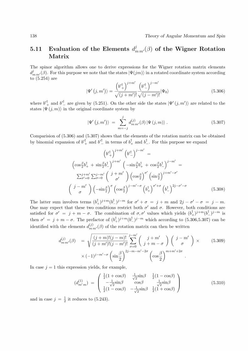
138 Theory of Angular Momentum and Spin
5.11 Evaluation of the Elements djmm′(β) of the Wigner RotationMatrix
The spinor algorithm allows one to derive expressions for the Wigner rotation matrix elementsdjmm′(β). For this purpose we note that the states |Ψ(jm)〉 in a rotated coordinate system accordingto (5.254) are
|Ψ′(j,m′
)〉 =
(b′†+
)j+m′√
(j +m′)!
(b′†−
)j−m′√
(j −m′)!|Ψ0〉 (5.306)
where b′†+ and b′†− are given by (5.251). On the other side the states |Ψ′ (j,m′)〉 are related to thestates |Ψ (j,m)〉 in the original coordinate system by
|Ψ′(j,m′
)〉 =
j∑m=−j
d(j)mm′(β) |Ψ (j,m)〉 . (5.307)
Comparision of (5.306) and (5.307) shows that the elements of the rotation matrix can be obtainedby binomial expansion of b′†+ and b′†− in terms of b†+ and b†−. For this purpose we expand(
b′†+
)j+m′ (b′†−
)j−m′=(
cosβ2 b†+ + sinβ2 b
†−
)j+m′ (−sinβ2 b
†+ + cosβ2 b
†−
)j−m′=∑j+m′
σ′=0
∑j−m′σ=0
(j +m′
σ′
)(cosβ2
)σ′ (sinβ2
)j+m′−σ′(j −m′σ
)(−sinβ2
)σ (cosβ2
)j−m′−σ (b†+
)σ′+σ (b†−
)2j−σ′−σ(5.308)
The latter sum involves terms (b†+)j+m(b†−)j−m for σ′ + σ = j + m and 2j − σ′ − σ = j − m.One may expect that these two conditions restrict both σ′ and σ. However, both conditions aresatisfied for σ′ = j + m − σ. The combination of σ, σ′ values which yields (b†+)j+m(b†−)j−m isthen σ′ = j + m − σ. The prefactor of (b†+)j+m(b†−)j−m which according to (5.306,5.307) can beidentified with the elements d(j)
mm′(β) of the rotation matrix can then be written
d(j)mm′(β) =
√(j +m)!(j −m)!(j +m′)!(j −m′)!
j−m′∑σ=0
(j +m′
j +m− σ
) (j −m′σ
)× (5.309)
× (−1)j−m′−σ(
sinβ
2
)2j−m−m′−2σ (cos
β
2
)m+m′+2σ
.
In case j = 1 this expression yields, for example,
(d(1)m′m) =
12(1 + cosβ) 1√
2sinβ 1
2(1− cosβ)− 1√
2sinβ cosβ 1√
2sinβ
12(1− cosβ) − 1√
2sinβ 1
2(1 + cosβ)
(5.310)
and in case j = 12 it reduces to (5.243).
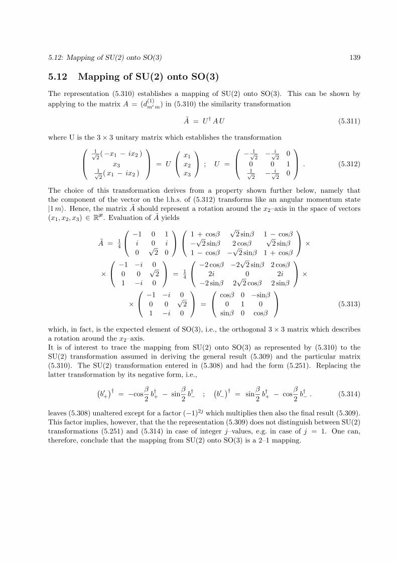
5.12: Mapping of SU(2) onto SO(3) 139
5.12 Mapping of SU(2) onto SO(3)
The representation (5.310) establishes a mapping of SU(2) onto SO(3). This can be shown byapplying to the matrix A = (d(1)
m′m) in (5.310) the similarity transformation
A = U †AU (5.311)
where U is the 3× 3 unitary matrix which establishes the transformation1√2(−x1 − ix2 )
x31√2(x1 − ix2 )
= U
x1
x2
x3
; U =
−1√2− i√
20
0 0 11√2− i√
20
. (5.312)
The choice of this transformation derives from a property shown further below, namely thatthe component of the vector on the l.h.s. of (5.312) transforms like an angular momentum state|1m〉. Hence, the matrix A should represent a rotation around the x2–axis in the space of vectors(x1, x2, x3) ∈ R3. Evaluation of A yields
A = 14
−1 0 1i 0 i
0√
2 0
1 + cosβ√
2 sinβ 1 − cosβ−√
2 sinβ 2 cosβ√
2 sinβ1 − cosβ −
√2 sinβ 1 + cosβ
××
−1 −i 00 0
√2
1 −i 0
= 14
−2 cosβ −2√
2 sinβ 2 cosβ2i 0 2i
−2 sinβ 2√
2 cosβ 2 sinβ
××
−1 −i 00 0
√2
1 −i 0
=
cosβ 0 −sinβ0 1 0
sinβ 0 cosβ
(5.313)
which, in fact, is the expected element of SO(3), i.e., the orthogonal 3× 3 matrix which describesa rotation around the x2–axis.It is of interest to trace the mapping from SU(2) onto SO(3) as represented by (5.310) to theSU(2) transformation assumed in deriving the general result (5.309) and the particular matrix(5.310). The SU(2) transformation entered in (5.308) and had the form (5.251). Replacing thelatter transformation by its negative form, i.e.,(
b′+)† = −cos
β
2b†+ − sin
β
2b†− ;
(b′−)† = sin
β
2b†+ − cos
β
2b†− . (5.314)
leaves (5.308) unaltered except for a factor (−1)2j which multiplies then also the final result (5.309).This factor implies, however, that the the representation (5.309) does not distinguish between SU(2)transformations (5.251) and (5.314) in case of integer j–values, e.g. in case of j = 1. One can,therefore, conclude that the mapping from SU(2) onto SO(3) is a 2–1 mapping.

140 Theory of Angular Momentum and Spin
Chapter 6
Quantum Mechanical Addition ofAngular Momenta and Spin
In this section we consider composite systems made up of several particles, each carrying orbitalangular momentum decribed by spherical harmonics Y`m(θ, φ) as eigenfunctions and/or spin. Oftenthe socalled total angular momentum, classically speaking the sum of all angular momenta and spinsof the composite system, is the quantity of interest, since related operators, sums of orbital angularmomentum and of spin operators of the particles, commute with the Hamiltonian of the compositesystem and, hence, give rise to good quantum numbers. We like to illustrate this for an exampleinvolving particle motion. Further below we will consider composite systems involving spin states.
Example: Three Particle Scattering
Consider the scattering of three particles A, B, C governed by a Hamiltonian H which dependsonly on the internal coordinates of the system, e.g., on the distances between the three particles,but neither on the position of the center of mass of the particles nor on the overall orientation ofthe three particle system with respect to a laboratory–fixed coordinate frame.To specify the dependency of the Hamiltonian on the particle coordinates we start from the ninenumbers which specify the Cartesian components of the three position vectors ~rA, ~rB, ~rC of theparticles. Since the Hamiltonian does not depend on the position of the center of mass ~R =(mA~rA + mB~rB + mC~rC)/(mA+mB+mC), six parameters must suffice to describe the interactionof the system. The overall orientation of any three particle configuration can be specified bythree parameters1, e.g., by a rotational vector ~ϑ. This eleminates three further parameters fromthe dependency of the Hamiltonian on the three particle configuration and one is left with threeparameters. How should they be chosen?Actually there is no unique choice. We like to consider a choice which is physically most reasonablein a situation that the scattering proceeds such that particles A and B are bound, and particle Cimpinges on the compound AB coming from a large distance. In this case a proper choice for adescription of interactions would be to consider the vectors ~rAB = ~rA − ~rB and ~ρC = (mA~rA +mB~rB)/(mA +mB)− ~rC , and to express the Hamiltonian in terms of |~rAB|, |~ρC |, and ^(~rAB, ~ρC).The rotational part of the scattering motion is described then in terms of the unit vectors rAB and
1We remind the reader that, for example, three Eulerian angles α, β, γ are needed to specify a general rotationaltransformation
141

142 Addition of Angular Momenta and Spin
ρC , each of which stands for two angles. One may consider then to describe the motion in termsof products of spherical harmonics Y`1m1(rAB)Y`2m2(ρC) describing rotation of the compound ABand the orbital angular momentum of C around AB.One can describe the rotational degrees of freedom of the three-particle scattering process throughthe basis
B = Y`1m1(rAB)Y`2m2(ρC), `1 = 0, 1, . . . , `1,max,−`1 ≤ m1 ≤ `1;`2 = 0, 1, . . . , `2,max,−`2 ≤ m1 ≤ `2 (6.1)
where `1,max and `2,max denote the largest orbital and rotational angular momentum values, thevalues of which are determined by the size of the interaction domain ∆V , by the total energy E,by the masses mA, mB, mC , and by the moment of inertia IA−B of the diatomic molecule A–Bapproximately as follows
`1,max =∆~
√2mAmBmC E
mAmB + mBmC + mAmC, `2,max =
1~
√2 IA−BE . (6.2)
The dimension d(B) of B is
d(B) =`1,max∑`1=0
(2 `1 + 1)`2,max∑`2=0
(2 `2 + 1) = (`1,max + 1)2 (`2,max + 1)2 (6.3)
For rather moderate values `1,max = `2,max = 10 one obtains d(B) = 14 641, a very large number.Such large number of dynamically coupled states would constitute a serious problem in any detaileddescription of the scattering process, in particular, since further important degrees of freedom, i.e.,vibrations and rearrangement of the particles in reactions like AB + C → A + BC, have noteven be considered. The rotational symmetry of the interaction between the particles allows one,however, to separate the 14 641 dimensional space of rotational states Y`1m1(rAB)Y`2m2(ρC) intosubspaces Bk, B1⊕B2⊕ . . . = B such, that only states within the subspaces Bk are coupled in thescattering process. In fact, as we will demonstrate below, the dimensions d(Bk) of these subspacesdoes not exceed 100. Such extremely useful transformation of the problem can be achieved throughthe choice of a new basis set
B′ = ∑`1,m1`2,m2
c(n)`1,m1;`2,m2
Y`1m1(rAB)Y`2m2(ρC), n = 1, 2, . . . 14 641 . (6.4)
The basis set which provides a maximum degree of decoupling between rotational states is of greatprinciple interest since the new states behave in many respects like states with the attributesof a single angular momentum state: to an observer the three particle system prepared in suchstates my look like a two particle system governed by a single angular momentum state. Obviously,composite systems behaving like elementary objects are common, albeit puzzling, and the followingmathematical description will shed light on their ubiquitous appearence in physics, in fact, will maketheir appearence a natural consequence of the symmetry of the building blocks of matter.There is yet another important reason why the following section is of fundamental importance forthe theory of the microscopic world governed by Quantum Mechanics, rather than by ClassicalMechanics. The latter often arrives at the physical properties of composite systems by adding the

6.0: Addition of Angular Momenta and Spin 143
corresponding physical properties of the elementary components; examples are the total momentumor the total angular momentum of a composite object which are the sum of the (angular) momentaof the elementary components. Describing quantum mechanically a property of a composite objectas a whole and relating this property to the properties of the elementary building blocks is then thequantum mechanical equivalent of the important operation of addittion. In this sense, the readerwill learn in the following section how to add and subtract in the microscopic world of QuantumPhysics, presumably a facility the reader would like to acquire with great eagerness.
Rotational Symmetry of the Hamiltonian
As pointed out already, the existence of a basis (6.4) which decouples rotational states is connectedwith the rotational symmetry of the Hamiltonian of the three particle system considered, i.e.,connected with the fact that the Hamiltonian H does not depend on the overall orientation of thethree interacting particles. Hence, rotations R(~ϑ) of the wave functions ψ(~rAB, ~ρC) defined through
R(~ϑ)ψ(~rAB, ~ρC) = ψ(R−1(~ϑ)~rAB, R−1(~ϑ) ~ρC) (6.5)
do not affect the Hamiltonian. To specify this property mathematically let us denote by H′ theHamiltonian in the rotated frame, assuming presently that H′ might, in fact, be different from H.It holds then H′R(~ϑ)ψ = R(~ϑ) Hψ. Since this is true for any ψ(~rAB, ~ρC) it follows H′R(~ϑ) =R(~ϑ) H, from which follows in turn the well-known result that H′ is related to H through thesimilarity transformation H′ = R(~ϑ) H R−1(~ϑ). The invariance of the Hamiltonian under overallrotations of the three particle system implies then
H = R(~ϑ) H R−1(~ϑ) . (6.6)
For the following it is essential to note that H is not invariant under rotations of only ~rAB or ~ρC ,but solely under simultaneous and identical rotations of ~rAB or ~ρC .Following our description of rotations of single particle wave functions we express (6.5) accordingto (5.48)
R(~ϑ) = exp(− i
~
~ϑ · ~J (1)
)exp
(− i
~
~ϑ · ~J (2)
)(6.7)
where the generators ~J (k) are differential operators acting on rAB (k = 1) and on ρC (k = 2). Forexample, according to (5.53, 5.55) holds
− i~
J (1)1 = zAB
∂
∂yAB− yAB
∂
∂zAB; − i
~
J (2)3 = ρy
∂
∂ρx− ρx
∂
∂ρy. (6.8)
Obviously, the commutation relationships[J (1)p , J (2)
q
]= 0 for p, q = 1, 2, 3 (6.9)
hold since the components of ~J (k) are differential operators with respect to different variables. Onecan equivalently express therefore (6.7)
R(~ϑ) = exp(− i
~
~ϑ ·~J)
(6.10)

144 Addition of Angular Momenta and Spin
where~J = ~J (1) + ~J (2) . (6.11)
By means of (6.11) we can write the condition (6.6) for rotational invariance of the Hamiltonian inthe form
H = exp(− i~
~ϑ ·~J)
H exp(
+i
~
~ϑ ·~J)
. (6.12)
We consider this equation for infinitesimal rotations, i.e. for |~ϑ| 1. To order O(|~ϑ|) one obtains
H ≈(
11 − i
~
~ϑ ·~J)
H(
11 +i
~
~ϑ ·~J)≈ H +
i
~
H ~ϑ ·~J − i
~
~ϑ ·~JH . (6.13)
Since this holds for any ~ϑ it follows H~J − ~JH = 0 or, componentwise,
[H, Jk] = 0 , k = 1, 2, 3 . (6.14)
We will refer in the following to Jk, k = 1, 2, 3 as the three components of the total angularmomentum operator.The property (6.14) implies that the total angular momentum is conserved during the scatteringprocess, i.e., that energy, and the eigenvalues of ~J2 and J3 are good quantum numbers. To describethe scattering process of AB + C most concisely one seeks eigenstates YJM of ~J2 and J3 which canbe expressed in terms of Y`1m1(rAB)Y`2m2(ρC).
Definition of Total Angular Momentum States
The commutation property (6.14) implies that the components of the total angular momentumoperator (6.12) each individually can have simultaneous eigenstates with the Hamiltonian. Wesuspect, of course, that the components Jk, k = 1, 2, 3 cannot have simultaneous eigenstates amongeach other, a supposition which can be tested through the commutation properties of these opera-tors. One can show readily that the commutation relationships
[Jk, J`] = i~ εk`mJm (6.15)
are satisfied, i.e., the operators Jk, k = 1, 2, 3 do not commute. For a proof one uses (6.9), theproperties [J (n)
k ,J (n)` ] = i~ εk`mJ
(n)m for n = 1, 2 together with the property [A,B + C] =
[A,B] + [A,C].We recognize, however, the important fact that the Jk obey the Lie algebra of SO(3). Accordingto the theorem above this property implies that one can construct eigenstates YJM of J3 and of
J2 = J
21 + J
22 + J
23 (6.16)
following the procedure stated in the theorem above [c.f. Eqs. (5.71–5.81)]. In fact, we will findthat the states yield the basis B′ with the desired property of a maximal uncoupling of rotationalstates.Before we apply the procedure (5.71–5.81) we want to consider the relationship between YJM andY`1m1(rAB)Y`2m2(ρC). In the following we will use the notation
Ω1 = rAB , Ω2 = ρC . (6.17)

6.1: Clebsch-Gordan Coefficients 145
6.1 Clebsch-Gordan Coefficients
In order to determine YJM we notice that the states Y`1m1(Ω1)Y`2m2(Ω2) are characterized by fourquantum numbers corresponding to eigenvalues of
[J (1)
]2, J (1)
3 ,[J (2)
]2, and J (2)
3 . Since YJM
sofar specifies solely two quantum numbers, two further quantum numbers need to be specifiedfor a complete characterization of the total angular momentum states. The two missing quantumnumbers are `1 and `2 corresponding to the eigenvalues of
[J (1)
]2and
[J (2)
]2. We, therefore,
assume the expansion
YJM (`1, `2|Ω1,Ω2) =∑m1,m2
(J M |`1m1 `2m2)Y`1m1(Ω1)Y`2m2(Ω2) (6.18)
where the states YJM (`1, `2|Ω1, ρC) are normalized. The expansion coefficients (J M |`1m1 `2m2)are called the Clebsch-Gordan coefficients which we seek to determine now. These coefficients,or the closely related Wigner 3j-coefficients introduced further below, play a cardinal role in themathematical description of microscopic physical systems. Equivalent coefficients exist for othersymmetry properties of multi–component systems, an important example being the symmetrygroups SU(N) governing elementary particles made up of two quarks, i.e., mesons, and three quarks,i.e., baryons.
Exercise 6.1.1: Show that J2, J3,(J (1)
)2,(J (2)
)2, and ~J (1) · ~J (2) commute. Why can states YJM
then not be specified by 5 quantum numbers?
Properties of Clebsch-Gordan Coefficients
A few important properties of Clebsch-Gordan coefficients can be derived rather easily. We firstnotice that YJM in (6.18) is an eigenfunction of J3, the eigenvalue being specified by the quantumnumber M , i.e.
J3 YJM = ~M YJM . (6.19)
Noting J3 = J (1)3 + J (2)
3 and applying this to the l.h.s. of (6.18) yields using the propertyJ (k)
3 Y`kmk(Ωk) = ~mk Y`kmk(Ωk) , k = 1, 2
M YJM (`1, `2|Ω1,Ω2) =∑m1,m2
(m1 + m2) (J M |`1m1 `2m2)Y`1m1(Ω1)Y`2m2(Ω2) . (6.20)
This equation can be satisfied only if the Clebsch-Gordan coefficients satisfy
(J M |`1m1 `2m2) = 0 for m1 + m2 6= M . (6.21)
One can, hence, restrict the sum in (6.18) to avoid summation of vanishing terms
YJM (`1, `2|Ω1,Ω2) =∑m1
(J M |`1m1 `2M −m1)Y`1m1(Ω1)Y`2m2(Ω2) . (6.22)
We will not adopt such explicit summation since it leads to cumbersum notation. However, thereader should always keep in mind that conditions equivalent to (6.21) hold.

146 Theory of Angular Momentum and Spin
The expansion (6.18) constitutes a change of an orthonormal basis
B(`1, `2) = Y`1m1(Ω1)Y`2m2(Ω2),m1 = −`1,−`1 + 1, . . . , `1 ,m2 = −`2,−`2 + 1, . . . , `2 , (6.23)
corresponding to the r.h.s., to a new basis B′(`1, `2) corresponding to the l.h.s. The orthonormalityproperty implies∫
dΩ1
∫dΩ2 Y`1m1(Ω1)Y`2m2(Ω2)Y`′1m′1Ω1)Y`′2m′2(Ω2) = δ`1`′1δm1m′1
δ`2`′2δm2m′2. (6.24)
The basis B(`1, `2) has (2`1 + 1)(2`2 + 1) elements. The basis B′(`1, `2) is also orthonormal2 andmust have the same number of elements. For each quantum number J there should be 2J + 1elements YJM with M = −J,−J + 1, . . . , J . However, it is not immediately obvious what the J–values are. Since YJM represents the total angular momentum state and Y`1m1(Ω1) and Y`2m2(Ω2)the individual angular momenta one may start from one’s classical notion that these states representangular momentum vectors ~J , ~J (1) and ~J (2), respectively. In this case the range of | ~J |–values wouldbe the interval [
∣∣∣| ~J (1)| − | ~J (2)|∣∣∣ , | ~J (1)| + | ~J (2)|]. This obviously corresponds quantum mechanically
to a range of J–values J = |`1 − `2|, |`1 − `2|+ 1, . . . `1 + `2. In fact, it holds
`1+`2∑J=|`1−`2|
( 2J + 1 ) = (2`1 + 1) (2`2 + 1) , (6.25)
i.e., the basis B′(`1, `2) should be
B2 = YJM (`1, `2|Ω1,Ω2); J = |`1 − `2|, |`1 − `2|+ 1, `1 + `2 ,
M = −J,−J + 1, . . . , J . (6.26)
We will show below in an explicit construction of the Clebsch-Gordan coefficients that, in fact, therange of values assumed for J is correct. Our derivation below will also yield real values for theClebsch-Gordan coefficients.
Exercise 6.1.2: Prove Eq. (6.25)
We want to state now two summation conditions which follow from the orthonormality of the twobasis sets B(`1, `2) and B′(`1, `2). The property∫
dΩ1
∫dΩ2 Y∗JM (`1, `2|Ω1,Ω2) YJ ′M ′(`1, `2|Ω1,Ω2) = δJJ ′δMM ′ (6.27)
together with (6.18) applied to Y∗JM and to YJ ′M ′ and with (6.24) yields∑m1,m2
(J M |`1m1 `2m2)∗(J ′M ′|`1m1 `2m2) = δJJ ′δMM ′ . (6.28)
2This property follows from the fact that the basis elements are eigenstates of hermitian operators with differenteigenvalues, and that the states can be normalized.
6.2: Construction of Clebsch-Gordan Coefficients 147
The second summation condition starts from the fact that the basis sets B(`1, `2) and B′(`1, `2)span the same function space. Hence, it is possible to expand Y`1m1(Ω1)Y`2m2(Ω2) in terms ofYJM (`1, `2|Ω1,Ω2), i.e.,
Y`1m1(Ω1)Y`2m2(Ω2) =`1+`2∑
J ′=|`1−`2|
J∑M ′=−J
cJ ′M ′ YJ ′M ′(`1, `2|Ω1,Ω2) , (6.29)
where the expansion coefficients are given by the respective scalar products in function space
cJ ′M ′ =∫dΩ1
∫dΩ2 Y∗J ′M ′(`1, `2|Ω1,Ω2)Y`1m1(Ω1)Y`2m2(Ω2) . (6.30)
The latter property follows from multiplying (6.18) by Y∗J ′M ′(`1, `2|Ω1,Ω2) and integrating. Theorthogonality property (6.27) yields
δJJ ′δMM ′ =∑m1,m2
(J M |`1m1 `2m2) cJ ′M ′ . (6.31)
Comparision with (6.28) allows one to conclude that the coefficients cJ ′M ′ are identical to(J ′M ′|`1m1 `2m2)∗, i.e.,
Y`1m1(Ω1)Y`2m2(Ω2)
=`1+`2∑
J ′=|`1−`2|
J∑M ′=−J
(J ′M ′|`1m1 `2m2)∗YJ ′M ′(`1, `2|Ω1,Ω2) , (6.32)
which complements (6.18). One can show readily using the same reasoning as applied in thederivation of (6.28) from (6.18) that the Clebsch-Gordan coefficients obey the second summationcondition ∑
JM
(J M |`1m1 `2m2)∗(J M |`1m′1 `2m′2) = δm1m′1δm2m′2
. (6.33)
The latter summation has not been restricted explicitly to allowed J–values, rather the convention
(J M |`1m1 `2m2) = 0 if J < |`1 − `2| , or J > `1 + `2 (6.34)
has been assumed.
6.2 Construction of Clebsch-Gordan Coefficients
We will now construct the Clebsch-Gordan coefficients. The result of this construction will includeall the properties previewed above. At this point we like to stress that the construction will be basedon the theorems (5.71–5.81) stated above, i.e., will be based solely on the commutation properties ofthe operators ~J and ~J (k). We can, therefore, also apply the results, and actually also the propertiesof Clebsch-Gordan coefficients stated above, to composite systems involving spin-1
2 states. A similarconstruction will also be applied to composite systems governed by other symmetry groups, e.g.,the group SU(3) in case of meson multiplets involving two quarks, or baryons multiplets involvingthree quarks.
148 Addition of Angular Momenta and Spin
For the construction of YJM we will need the operators
J± = J1 + iJ2 . (6.35)
The construction assumes a particular choice of J ∈ |`1 − `2|, |`1 − `2| + 1, . . . `1 + `2 and forsuch J–value seeks an expansion (6.18) which satisfies
J+ YJJ(`1, `2|Ω1,Ω2) = 0 (6.36)J3 YJJ(`1, `2|Ω1,Ω2) = ~ J YJJ(`1, `2|Ω1,Ω2) . (6.37)
The solution needs to be normalized. Having determined such YJJ we then construct the wholefamily of functions XJ = YJM (`1, `2|Ω1,Ω2), M = −J,−J + 1, . . . J by applying repeatedly
J−YJM+1(`1, `2|Ω1,Ω2) = ~
√(J +M + 1)(J −M)YJM (`1, `2|Ω1,Ω2) . (6.38)
for M = J − 1, J − 2, . . . ,−J .We embark on the suggested construction for the choice J = `1 + `2. We first seek an unnormalizedsolution GJJ and later normalize. To find GJJ we start from the observation that GJJ represents thestate with the largest possible quantum number J = `1 + `2 with the largest possible componentM = `1 + `2 along the z–axis. The corresponding classical total angular momentum vector ~Jclass
would be obtained by aligning both ~J (1)class and ~J (2)
class also along the z–axis and adding these twovectors. Quantum mechanically this corresponds to a state
G`1+`2,`1+`2(`1, `2|Ω1,Ω2) = Y`1`1(Ω1)Y`2`2(Ω2) (6.39)
which we will try for a solution of (6.37). For this purpose we insert (6.39) into (6.37) and replaceaccording to (6.11) J+ by J (1)
+ + J (2)+ . We obtain using (5.66,5.68)(
J (1)+ + J (2)
+
)Y`1`1(Ω1)Y`2`2(Ω2) (6.40)
=(J (1)
+ Y`1`1(Ω1))Y`2`2(Ω2) + Y`1`1(Ω1)
(J (2)
+ Y`2`2(Ω2))
= 0 .
Similarly, we can demonstrate condition (6.25) using (6.11) and (5.64)(J (1)
3 + J (2)3
)Y`1`1(Ω1)Y`2`2(Ω2)
=(J (1)
3 Y`1`1(Ω1))Y`2`2(Ω2) + Y`1`1(Ω1)
(J (2)
3 Y`2`2(Ω2))
= ~ (`1 + `2)Y`1`1(Ω1)Y`2`2(Ω2) . (6.41)
In fact, we can also demonstrate using (??) that G`1+`2,`1+`2(`1, `2|Ω1,Ω2) is normalized∫dΩ1
∫dΩ2 G`1+`2,`1+`2(`1, `2|Ω1,Ω2)
=(∫
dΩ1Y`1`1(Ω1)) (∫
dΩ2Y`2`2(Ω2))
= 1 . (6.42)
We, therefore, have shown
Y`1+`2,`1+`2(`1, `2|Ω1,Ω2) = Y`1`1(Ω1)Y`2`2(Ω2) . (6.43)

6.2: Construction of Clebsch-Gordan Coefficients 149
We now employ property (6.38) to construct the family of functions B`1+`2 =Y`1+`2M(`1, `2|1,2), M = −(`1 + `2), . . . , (`1 + `2). We demonstrate the procedure ex-plicitly only for M = `1 + `2 − 1. The r.h.s. of (6.38) yields with J− = J (1)
− + J (1)− the ex-
pression ~√
2`1 Y`1`1−1(Ω1)Y`2`2(Ω2) + ~
√2`2 Y`1`1−1(Ω1)Y`2`2−1(Ω2). The l.h.s. of (6.38) yields
~
√2(`1 + `2)Y`1+`2`1+`2−1(`1, `2|Ω1,Ω2). One obtains then
Y`1+`2 `1+`2−1(`1, `2|Ω1,Ω2) = (6.44)√`1
`1+`2Y`1`1−1(Ω1)Y`2`2(Ω2) +
√`2
`1+`2Y`1`1(Ω1)Y`2`2−1(Ω2) .
This construction can be continued to obtain all 2(`1 + `2) + 1 elements of B`1+`2 and, thereby,all the Clebsch-Gordan coefficients (`1 + `2M |`1m1`2m2). We have provided in Table 1 the explicitform of YJ M (`1`2|Ω1Ω2) for `1 = 2 and `2 = 1 to illustrate the construction. The reader shouldfamiliarize himself with the entries of the Table, in particular, with the symmetry pattern and withthe terms Y`1m1Y`2m2 contributing to each YJ M .We like to construct now the family of total angular momentum functions B`1+`2−1 =Y`1+`2−1M(`1, `2|1,2), M = −(`1 + `2 − 1), . . . , (`1 + `2 − 1). We seek for this pur-pose first an unnormalized solution G`1+`2−1 `1+`2−1 of (6.36, 6.37). According to the condition(6.21) we set
G`1+`2−1 `1+`2−1(`1`2|Ω1Ω2) = Y`1`1−1(Ω1)Y`2`2(Ω2) + c Y`1`1(Ω1)Y`2`2−1(Ω2) (6.45)
for some unknown constant c. One can readily show that (6.37) is satisfied. To demonstrate (6.36)we proceed as above and obtain(
J (1)+ Y`1`1−1(Ω1)
)Y`2`2(Ω2) + c Y`1`1(Ω1)
(J (2)
+ Y`2`2−1(Ω2))
=(√
2`1 + c√
2`2)Y`1`1(Ω1)Y`2`2(Ω2) = 0 . (6.46)
To satisfy this equation one needs to choose c = −√`1/`2. We have thereby determined
G`1+`2−1 `1+`2−1 in (6.45). Normalization yields furthermore
Y`1+`2−1 `1+`2−1(`1`2|Ω1Ω2) (6.47)
=√
`2`1 + `2
Y`1`1−1(Ω1)Y`2`2(Ω2) −√
`1`1 + `2
Y`1`1(Ω1)Y`2`2−1(Ω2) .
This expression is orthogonal to (6.39) as required by (6.27).Expression (6.47) can serve now to obtain recursively the elements of the family B`1+`2−1 forM = `1 + `2−2, `1 + `2−3, . . . ,−(`1 + `2−1). Having constructed this family we have determinedthe Clebsch-Gordan coefficients (`1 + `2 − 1M |`1m1`2m2). The result is illustrated for the case`1 = 2, `2 = 1 in Table 1.One can obviously continue the construction outlined to determine Y`1+`2−2 `1+`2−2, etc. and alltotal angular momentum functions for a given choice of `1 and `2.
Exercise 6.2.1: Construct following the procedure above the three functions YJM (`1, `2|Ω1,Ω2)for M = `1 + `2 − 2 and J = `1 + `2, `1 + `2 − 1, `1 + `2 − 2. Show that the resulting functionsare orthonormal.
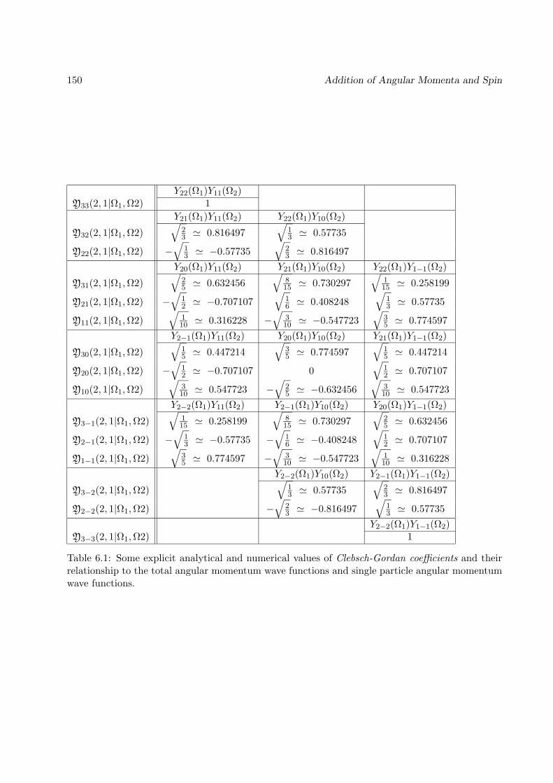
150 Addition of Angular Momenta and Spin
Y22(Ω1)Y11(Ω2)Y33(2, 1|Ω1,Ω2) 1
Y21(Ω1)Y11(Ω2) Y22(Ω1)Y10(Ω2)
Y32(2, 1|Ω1,Ω2)√
23 ' 0.816497
√13 ' 0.57735
Y22(2, 1|Ω1,Ω2) −√
13 ' −0.57735
√23 ' 0.816497
Y20(Ω1)Y11(Ω2) Y21(Ω1)Y10(Ω2) Y22(Ω1)Y1−1(Ω2)
Y31(2, 1|Ω1,Ω2)√
25 ' 0.632456
√815 ' 0.730297
√115 ' 0.258199
Y21(2, 1|Ω1,Ω2) −√
12 ' −0.707107
√16 ' 0.408248
√13 ' 0.57735
Y11(2, 1|Ω1,Ω2)√
110 ' 0.316228 −
√310 ' −0.547723
√35 ' 0.774597
Y2−1(Ω1)Y11(Ω2) Y20(Ω1)Y10(Ω2) Y21(Ω1)Y1−1(Ω2)
Y30(2, 1|Ω1,Ω2)√
15 ' 0.447214
√35 ' 0.774597
√15 ' 0.447214
Y20(2, 1|Ω1,Ω2) −√
12 ' −0.707107 0
√12 ' 0.707107
Y10(2, 1|Ω1,Ω2)√
310 ' 0.547723 −
√25 ' −0.632456
√310 ' 0.547723
Y2−2(Ω1)Y11(Ω2) Y2−1(Ω1)Y10(Ω2) Y20(Ω1)Y1−1(Ω2)
Y3−1(2, 1|Ω1,Ω2)√
115 ' 0.258199
√815 ' 0.730297
√25 ' 0.632456
Y2−1(2, 1|Ω1,Ω2) −√
13 ' −0.57735 −
√16 ' −0.408248
√12 ' 0.707107
Y1−1(2, 1|Ω1,Ω2)√
35 ' 0.774597 −
√310 ' −0.547723
√110 ' 0.316228
Y2−2(Ω1)Y10(Ω2) Y2−1(Ω1)Y1−1(Ω2)
Y3−2(2, 1|Ω1,Ω2)√
13 ' 0.57735
√23 ' 0.816497
Y2−2(2, 1|Ω1,Ω2) −√
23 ' −0.816497
√13 ' 0.57735
Y2−2(Ω1)Y1−1(Ω2)Y3−3(2, 1|Ω1,Ω2) 1
Table 6.1: Some explicit analytical and numerical values of Clebsch-Gordan coefficients and theirrelationship to the total angular momentum wave functions and single particle angular momentumwave functions.

6.3: Explicit Expressions of CG–Coefficients 151
Exercise 6.2.2: Use the construction for Clebsch-Gordan coefficients above to prove the followingformulas
〈J,M |`,m− 12, 1
2,+ 1
2〉 =
√
J+M2J for ` = J − 1
2
−√
J−M+12J+2 for ` = J + 1
2
〈J,M |`,m+ 12, 1
2,− 1
2〉 =
√
J−M2J for ` = J − 1
2√J+M+1
2J+2 for ` = J + 12
.
The construction described provides a very cumbersome route to the analytical and numericalvalues of the Clebsch-Gordan coefficients. It is actually possible to state explicit expressions forany single coefficient (JM |`1m1`2m2). These expressions will be derived now.
6.3 Explicit Expression for the Clebsch–Gordan Coefficients
We want to establish in this Section an explicit expression for the Clebsch–Gordan coefficients(JM |`1m1`2m2). For this purpsose we will employ the spinor operators introduced in Sections 5.9,5.10.
Definition of Spinor Operators for Two Particles
In contrast to Sections 5.9, 5.10 where we studied single particle angular momentum and spin, weare dealing now with two particles carrying angular momentum or spin. Accordingly, we extentdefinition (5.287) to two particles
(1)Jk = 12
∑ζ,ζ′ a
†ζ < ζ |σk| ζ ′ > aζ′ (6.48)
(2)Jk = 12
∑ζ,ζ′ b
†ζ < ζ |σk| ζ ′ > bζ′ (6.49)
where ζ, ζ ′ = ± and the matrix elements < ζ |σk| ζ ′ > are as defined in Section 5.10. The creationand annihilation operators are again of the boson type with commutation properties[
aζ , aζ′]
=[a†ζ , a
†ζ′
]= 0 ,
[aζ , a
†ζ′
]= δζζ′ (6.50)[
bζ , bζ′]
=[b†ζ , b
†ζ′
]= 0 ,
[bζ , b
†ζ′
]= δζζ′ . (6.51)
The operators aζ , a†ζ and bζ , b
†ζ refer to different particles and, hence, commute with each other[aζ , bζ′
]=[a†ζ , b
†ζ′
]=[aζ , b
†ζ′
]= 0 . (6.52)
According to Section 5.10 [cf. (5.254)] the angular momentum / spin eigenstates |`1m1〉1 and |`2m2〉2of the two particles are
|`1m1〉1 =
(a†+
)`1+m1
√(`1+m1)!
(a†−
)`1−m1
√(`1−m1)!
|Ψ0〉 (6.53)
|`2m2〉2 =
(b†+
)`2+m2
√(`2+m2)!
(b†−
)`2−m2
√(`2−m2)!
|Ψ0〉 . (6.54)
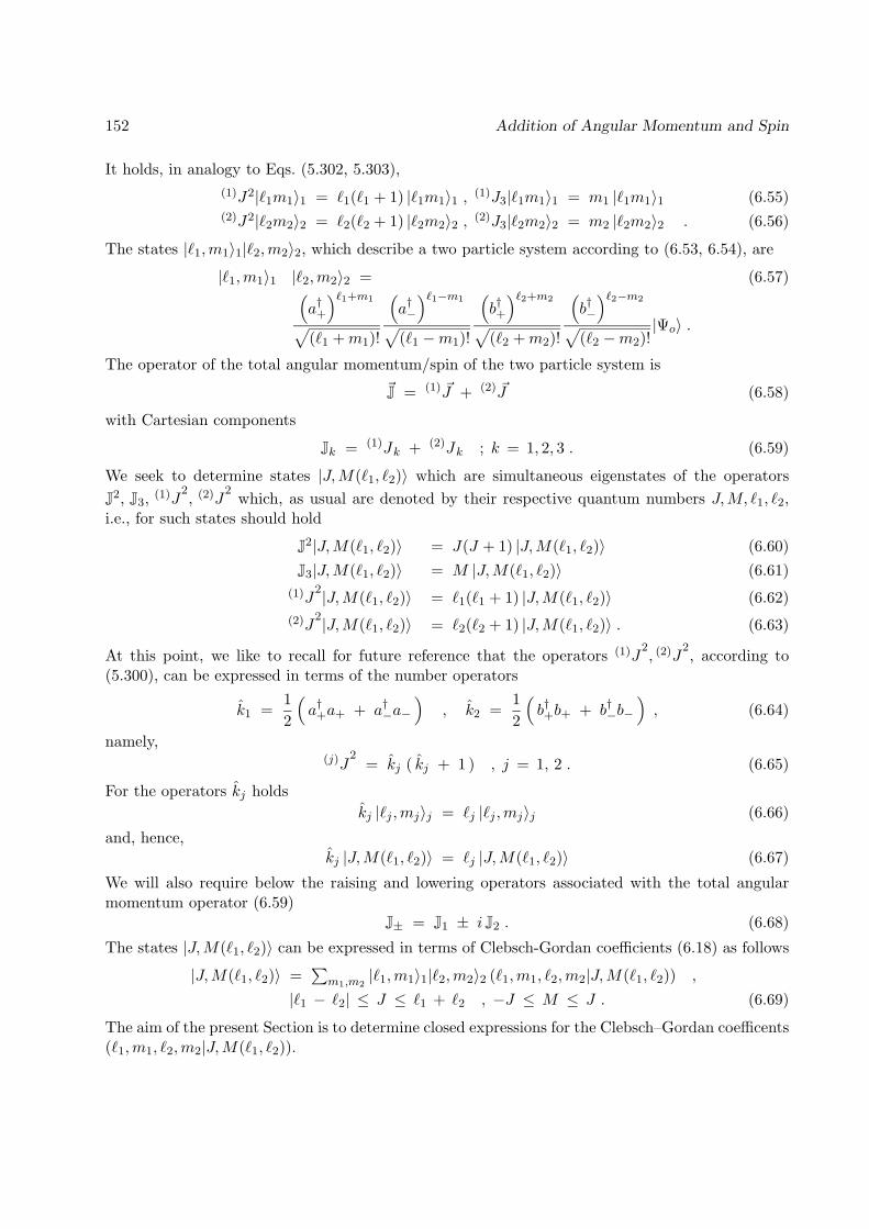
152 Addition of Angular Momentum and Spin
It holds, in analogy to Eqs. (5.302, 5.303),(1)J2|`1m1〉1 = `1(`1 + 1) |`1m1〉1 , (1)J3|`1m1〉1 = m1 |`1m1〉1 (6.55)(2)J2|`2m2〉2 = `2(`2 + 1) |`2m2〉2 , (2)J3|`2m2〉2 = m2 |`2m2〉2 . (6.56)
The states |`1,m1〉1|`2,m2〉2, which describe a two particle system according to (6.53, 6.54), are
|`1,m1〉1 |`2,m2〉2 = (6.57)(a†+
)`1+m1√(`1 +m1)!
(a†−
)`1−m1√(`1 −m1)!
(b†+
)`2+m2√(`2 +m2)!
(b†−
)`2−m2√(`2 −m2)!
|Ψo〉 .
The operator of the total angular momentum/spin of the two particle system is~J = (1) ~J + (2) ~J (6.58)
with Cartesian components
Jk = (1)Jk + (2)Jk ; k = 1, 2, 3 . (6.59)
We seek to determine states |J,M(`1, `2)〉 which are simultaneous eigenstates of the operatorsJ
2, J3,(1)J
2, (2)J
2which, as usual are denoted by their respective quantum numbers J,M, `1, `2,
i.e., for such states should hold
J2|J,M(`1, `2)〉 = J(J + 1) |J,M(`1, `2)〉 (6.60)J3|J,M(`1, `2)〉 = M |J,M(`1, `2)〉 (6.61)
(1)J2|J,M(`1, `2)〉 = `1(`1 + 1) |J,M(`1, `2)〉 (6.62)
(2)J2|J,M(`1, `2)〉 = `2(`2 + 1) |J,M(`1, `2)〉 . (6.63)
At this point, we like to recall for future reference that the operators (1)J2, (2)J
2, according to
(5.300), can be expressed in terms of the number operators
k1 =12
(a†+a+ + a†−a−
), k2 =
12
(b†+b+ + b†−b−
), (6.64)
namely,(j)J
2= kj ( kj + 1 ) , j = 1, 2 . (6.65)
For the operators kj holdskj |`j ,mj〉j = `j |`j ,mj〉j (6.66)
and, hence,kj |J,M(`1, `2)〉 = `j |J,M(`1, `2)〉 (6.67)
We will also require below the raising and lowering operators associated with the total angularmomentum operator (6.59)
J± = J1 ± i J2 . (6.68)
The states |J,M(`1, `2)〉 can be expressed in terms of Clebsch-Gordan coefficients (6.18) as follows
|J,M(`1, `2)〉 =∑
m1,m2|`1,m1〉1|`2,m2〉2 (`1,m1, `2,m2|J,M(`1, `2)) ,
|`1 − `2| ≤ J ≤ `1 + `2 , −J ≤ M ≤ J . (6.69)
The aim of the present Section is to determine closed expressions for the Clebsch–Gordan coefficents(`1,m1, `2,m2|J,M(`1, `2)).
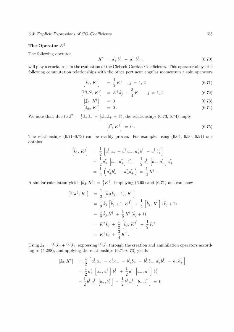
6.3: Explicit Expressions of CG–Coefficients 153
The Operator K†
The following operatorK† = a†+ b
†− − a†− b
†+ . (6.70)
will play a crucial role in the evaluation of the Clebsch-Gordan-Coefficients. This operator obeys thefollowing commutation relationships with the other pertinent angular momentum / spin operators[
kj , K†]
=12K† , j = 1, 2 (6.71)[
(j)J2, K†]
= K† kj +34K† , j = 1, 2 (6.72)[
J3, K†] = 0 (6.73)[
J±, K†] = 0 . (6.74)
We note that, due to J2 = 12J+J− + 1
2J−J+ + J23, the relationships (6.73, 6.74) imply[
J2, K†
]= 0 . (6.75)
The relationships (6.71–6.73) can be readily proven. For example, using (6.64, 6.50, 6.51) oneobtains [
k1, K†]
=12
[a†+a+ + a†−a−, a
†+b†− − a†−b
†+
]=
12a†+
[a+, a
†+
]b†− −
12a†−
[a−, a
†−
]b†+
=12
(a†+b
†− − a†−b
†+
)=
12K† .
A similar calculation yields [k2,K†] = 1
2K†. Employing (6.65) and (6.71) one can show[
(j)J2, K†]
=12
[kj(kj + 1), K†
]=
12kj
[kj + 1, K†
]+
12
[kj , K
†]
(kj + 1)
=12kjK
† +12K† (kj + 1)
= K† kj +12
[kj , K
†]
+12K†
= K† kj +34K† .
Using J3 = (1)J3 + (2)J3, expressing (k)J3 through the creation and annihilation operators accord-ing to (5.288), and applying the relationships (6.71–6.73) yields[
J3,K†] =
12
[a†+a+ − a†−a− + b†+b+ − b†−b−, a
†+b†− − a†−b
†+
]=
12a†+
[a+, a
†+
]b†− +
12a†−
[a−, a
†−
]b†+
− 12b†+a
†−
[b+, b
†+
]− 1
2b†−a
†+
[b−, b
†−
]= 0 .
154 Addition of Angular Momentum and Spin
Starting from (5.292) one can derive similarly[J+,K
†] =[a†+a− + b†+b−, a
†+b− − a†−b
†+
]= − a†+
[a−, a
†−
]b†+ + b†+a
†+
[b−, b
†−
]= 0 .
The property [J−, K†] = 0 is demonstrated in an analoguous way.
Action of K† on the states |J,M(`1, `2)〉
We want to demonstrate now that the action of K† on the states |J,M(`1, `2)〉 produces againtotal angular momentum eigenstates to the same J and M quantum numbers of J2 and J3, but fordifferent `1 and `2 quantum numbers of the operators (1)J2 and (2)J2.The commutation properties (6.73, 6.75) ascertain that under the action of K† the states|J,M(`1, `2)〉 remain eigenstates of J2 and J3 with the same quantum numbers. To demonstratethat the resulting states are eigenstates of (1)J2 and (2)J2 we exploit (6.72) and (6.62, 6.63, 6.67)
(j)J2K† |J,M(`1, `2)〉 =( [
(j)J2, K†]
+ K† (j)J2)|J,M(`1, `2)〉
=(K† kj +
34K† + K†`j (`j + 1)
)|J,M(`1, `2)〉
= K†(`j +
34
+ `j (`j + 1))|J,M(`1, `2)〉
=(`j +
12
)(`j +
32
)K† |J,M(`1, `2)〉 .
However, this result implies that K†|J,M(`1, `2)〉 is a state with quantum numbers `1 + 12 and
`2 + 12 , i.e., it holds
K† |J,M(`1, `2)〉 = N |J,M(`1 +12, `2 +
12
)〉 . (6.76)
Here N is an unknown normalization constant.One can generalize property (6.76) and state(
K†)n|J,M(`1, `2)〉 = N ′ |J,M(`1 +
n
2, `2 +
n
2)〉 (6.77)
where N ′ is another normalization constant. We consider now the case that (K†)n acts on thesimplest total angular momentum / spin state, namely, on the state
|j1 + j2, j1 + j2(j1, j2)〉 = |j1, j1〉1 |j2, j2〉2 , (6.78)
a state which has been used already in the construction of Clebsch-Gordan coefficients in Section 6.2.Application of (K†)n to this state yields, according to (6.77),
|j1 + j2, j1 + j2 (j1 +n
2, j2 +
n
2)〉 (6.79)
= N(n, j11 +n
2, j1 +
n
2)(K†)n|j1 + j2, j1 + j2(j1, j2)〉
6.3: Explicit Expressions of CG–Coefficients 155
where we denoted the associated normalization constant by N(n, j1 + n2 , j2 + n
2 ).It is now important to notice that any state of the type |J, J(`1, `2)〉 can be expressed through ther.h.s. of (6.79). For this purpose one needs to choose in (6.79) n, j1, j2 as follows
J = j1 + j2 , `1 = j1 +n
2, `2 = j2 +
n
2(6.80)
which is equivalent to
n = `1 + `2 − J
j1 = `1 −n
2=
12
(J + `1 − `2)
j2 = `2 −n
2=
12
(J + `1 − `2) . (6.81)
Accodingly, holds
|J, J(`1, `2)〉 = N(`1 + `2 − J, `1, `2)(K†)`1+`2−J
×
× |12
(J + `1 − `2) ,12
(J + `1 − `2)〉1 ×
× |12
(J + `2 − `1) ,12
(J + `2 − `1)〉2 . (6.82)
The normalization constant appearing here is actually
N(`1 + `2 − J, `1, `2) =[
(2J + 1)!(`1 + `2 − J)! (`1 + `2 + J + 1)!
] 12
. (6.83)
The derivation of this expression will be provided further below (see page 158 ff).
Strategy for Generating the States |J,M(`1, `2)〉
Our construction of the states |J,M(`1, `2)〉 exploits the expression (6.82) for |J, J(`1, `2)〉. Thelatter states, in analogy to the construction (5.104, 5.105) of the spherical harmonics, allow one toobtain the states |J,M(`1, `2)〉 for −J ≤ M ≤ J as follows
|J,M(`1, `2)〉 = ∆(J,M) (J−)J−M |J, J(`1, `2)〉 (6.84)
∆(J,M) =[
(J + M)!(2J)! (J − M)!
] 12
. (6.85)
Combining (6.84) with (6.82, 6.57) and exploiting the fact that J− and K† commute [c.f. (6.74)]yields
|J,M(`1, `2)〉 =N(`1 + `2 − J, `1, `2) ∆(J,M)√
(J + `1 − `2)! (J + `2 − `1)!× (6.86)
×(K†)`1+`2−J
(J−)J−M(a†+
)J+`1−`2 (b†+
)J+`2−`1|Ψo〉
156 Addition of Angular Momentum and Spin
Our strategy for the evaluation of the Clebsch-Gordan-coefficients is to expand (6.86) in terms ofmonomials (
a†+
)`1+m1(a†−
)`1−m1(b†+
)`2+m2(b†−
)`2−m2
|Ψo〉 , (6.87)
i.e., in terms of |`1,m1〉1|`2,m2〉2 [cf. (6.57)]. Comparision with (6.69) yields then the Clebsch-Gordan-coefficients.
Expansion of an Intermediate State
We first consider the expansion of the following factor appearing in (6.86)
|Grst〉 = Jr−
(a†+
)s (b†+
)t|Ψo〉 (6.88)
in terms of monomials (6.87). For this purpose we introduce the generating function
I(λ, x, y) = exp (λJ−) exp(x a†+
)exp
(x b†+
)|Ψo〉 . (6.89)
Taylor expansion of the two exponential operators yields immediately
I(λ, x, y) =∑r,s,t
λrxsyt
r!s!t!|Grst〉 , (6.90)
i.e., I(λ, x, y) is a generating function for the states |Grst〉 defined in (6.88).The desired expansion of |Grst〉 can be obtained from an alternate evaluation of I(λ, x, y) which isbased on the properties
aζf(a†ζ) |Ψo〉 =∂
∂a†ζf(a†ζ) |Ψo〉 bζf(b†ζ) |Ψo〉 =
∂
∂b†ζf(b†ζ) |Ψo〉 (6.91)
which, in analogy to (5.264), follows from the commutation properties (6.50–6.52). One obtainsthen using
J− = a†−a+ + b†−b+ (6.92)
and noting [a+, a†−] = [b+, b
†−] = 0 [cf. (6.50)]
exp (λJ− ) f(a†+) g(b†+) |Ψo〉 = exp(a†−a+
)f(a†+) exp
(b†b+
)g(b†+) |Ψo〉
=∑u
λu
u!
(a†−a+
)uf(a†+) ×
×∑v
λv
v!
(b†−b+
)vg(b†+) |Ψo〉
=∑u
(λ a†−
)uu!
(∂
∂a†+
)uf(a†+) ×
×∑v
(λ b†−
)vv!
(∂
∂b†+
)vg(b†+) |Ψo〉
= f(a†+ + λ a†−) g(b†+ + λ b†−) |Ψo〉 . (6.93)
6.3: Explicit Expressions of CG–Coefficients 157
We concludeI(λ, x, y) = exp
(a†+ + λ a†−
)exp
(b†+ + λ b†−
)|Ψo〉 . (6.94)
One can infer from this result the desired expressions for |Grst〉. Expanding the exponentials in(6.94) yields
I(λ, x, y) =∑s,t
xs
s!yt
t!
(a†+ + λ a†−
)s (b†+ + λ b†−
)t|Ψo〉
=∑s,t
xs
s!yt
t!
∑t
∑v
(su
)(tv
)×
×(a†+
)s−uλu(a†−
)u (b†+
)t−vλv(b†−
)v|Ψo〉
=∑r,s,t
λr
r!xs
s!yt
t!
∑q
r!(sq
)(t
r − q
)×
×(a†+
)s−q (a†−
)q (b†+
)t−r+q (b†−
)r−q|Ψo〉 (6.95)
Comparision with (6.90) allows one to infer
|Grs,t〉 =∑q
r!(sq
)(t
r − q
)×
×(a†+
)s−q (a†−
)q (b†+
)t−r+q (b†−
)r−q|Ψo〉 (6.96)
and, using the definition (6.88), one can write the right factor in (6.86)
(J−)J−M(a†+
)J+`1−`2 (b†+
)J+`2−`1|Ψo〉 (6.97)
=∑q
(J −M)!(J + `1 − `2)!(J + `2 − `1)!q!(J + `1 − `2 − q)!(J −M − q)!(M + `2 − `1 + q)!
×
×(a†+
)J+`1−`2−q (a†−
)q (b†+
)M+`2−`1+q (b†−
)J−M−q|Ψo〉
Final Result
Our last step is to apply the operator (K†)`1+`2−J to expression (6.97), to obtain the desiredexpansion of |J,M(`1, `2)〉 in terms of states |`1,m1〉1|`2,m2〉2. With K† given by (6.70) holds
(K†)`1+`2−J =
∑s
(`1 + `2 − J
s
)(−1)s (6.98)
(a†+
)`1+`2−J−s (b†−
)`1+`2−J−s (a†−
)s (b†+
)s.
Operation of this operator on (6.97) yields, using the commutation property (6.50),
|J,M(`1, `2)〉 =∑s,q
(−1)s (6.99)

158 Addition of Angular Momentum and Spin
(`1 + `2 − J)!(J −M)!(J + `1 − `2)!(J + `2 − `1)!s!(`1 + `2 − J − s)!q!(J + `1 − `2 − q)!(J −M − q)!(M + `2 − `1 + q)!(a†+
)2`1−q−s (a†−
)q+s (b†+
)M+`2−`1+q+s (b†−
)`1+`2−M−q−s|Ψo〉
The relationships (6.53,6.54) between creation operator monomials and angular momentum statesallow one to write this
|J,M(`1, `2)〉 =N(`1 + `2 − J, `1, `2) ∆(J,M)√
(J + `1 − `2)! (J + `2 − `1)!
∑s,q
(−1)s × (6.100)
× (`1 + `2 − J)!(J −M)!(J + `1 − `2)!(J + `2 − `1)!s!(`1 + `2 − J − s)!q!(J + `1 − `2 − q)!(J −M − q)!(M + `2 − `1 + q)!
×√
(2`1 − q − s)!(q + s)!×√
(M + `2 − `1 + q + s)!(`1 + `2 −M − q − s)!×|`1, `1 − q − s〉1 |`2,M − `1 + q + s〉2
One can conclude that this expression reproduces (6.69) if one identifies
m1 = `1 − q − s , m2 = M − `1 + q + s . (6.101)
Note that m1 + m2 = M holds. The summation over q corresponds then to the summationover m1, m2 in (6.69) since, according to (6.101), q = `1 − m1 − s and m2 = M − m1. TheClebsch-Gordan coefficents are then finally
(`1,m1, `2,m2|J,M) =
√2J + 1
[`1 + `2 − J)!(`1 − `2 + J)!(−`1 + `2 + J)!
(`1 + `2 + J + 1)!
] 12
× [(`1 +m1)!(`1 −m1)!(`2 +m2)!(`2 −m2)!(J +M)!(J −M)!]12
×∑s
(−1)s
s!(`1 −m1 − s)!(`2 +m2 − s)!
× 1(`1 + `2 − J − s)!(J − `1 −m2 + s)!(J − `2 +m1 + s)!
(6.102)
The Normalization
We want to determine now the expression (6.83) of the normalization constant N(`1 + `2−J, `1, `2)defined through (6.82). For this purpose we introduce
j1 =12
(J + `1 − `2) , j2 =12
(J + `2 − `1) , n = `1 + `2 − J . (6.103)
To determine N = N(`1+`2−J, `1, `2) we consider the scalar product 〈J, J(`1, `2)|J, J(`1, `2)〉 = 1.Using (6.82) and (6.103) this can be written
1 = N2 〈ψ(j1, j2, n)|ψ(j1, j2, n)〉 (6.104)

6.3: Explicit Expressions of CG–Coefficients 159
where|ψ(j1, j2, n)〉 =
(K†)n|j1, j1〉1|j2, j2〉2 . (6.105)
The first step of our calculation is the expansion of ψ(j1, j2, n) in terms of states |j′1,m1〉1|j′2,m2〉2.We employ the expression (6.57) for these states and the expression (6.70) for the operator K†.Accordingly, we obtain
|ψ(j1, j2, n)〉 =1√
(2j1)!(2j2)!
∑s
(ns
)(a†+b
†−
)n−s(−1)s
(a†−b
†+
)s(a†+
)2j1 (b†+
)2j2|Ψo〉 =
n!√(2j1)!(2j2)!
∑s
(−1)s√
(2j1 + n− s)!s!(2j2 + s)!(n− s)!s!(n− s)!(
a†+
)2j1−n−s (a†−
)s (b†+
)2j2+s (b†−
)n−s√
(2j1 + n− s)!s!(2j2 + s)!(n− s)!|Ψo〉 . (6.106)
The orthonormality of the states occurring in the last expression allows one to write (6.104)
1 = N2 (n!)2
(2j1)!(2j2)!
∑s
(2j1 + n− s)!(2j2 + s)!s!(n− s)!
= (n!)2∑s
(2j1 + n− s
2j1
)(2j2 + s
2j2
)(6.107)
The latter sum can be evaluated using(1
1 − λ
)n1+1
=∑m1
(n1 +m1
n1
)λm1 (6.108)
a property which follows from
∂ν
∂λν
(1
1 − λ
)n1+1∣∣∣∣∣λ=0
=(n1 + ν)!
n1!(6.109)
and Taylor expansion of the left hand side of (6.108). One obtains then, applying (6.108) twice,(1
1 − λ
)n1+1( 11 − λ
)n2+1
=∑m1,m2
(n1 +m1
n1
)(n2 +m2
n2
)λm1+m2 (6.110)
which can be written(1
1 − λ
)n1+n2+2
=∑r
[∑s
(n1 + r − s
n1
)(n2 + sn2
)]λr (6.111)
Comparision with (6.108) yields the identity∑s
(n1 + r − s
n1
)(n2 + sn2
)=(n1 + n2 + r + 1n1 + n2 + 1
). (6.112)

160 Theory of Angular Momentum and Spin
Applying this to (6.107) yields
1 = N2 (n!)2
(2j1 + 2j2 + n+ 1
2j1 + 2j2 + 1
)= N2 n!(2j1 + 2j2 + n+ 1)!
(2j1 + 2j2 + 1)!. (6.113)
Using the identities (6.103) one obtains the desired result (6.83).
6.4 Symmetries of the Clebsch-Gordan Coefficients
The Clebsch-Gordan coefficients obey symmetry properties which reflect geometrical aspects of theoperator relationship (6.11)
~J = ~J (1) + ~J (2) . (6.114)
For example, interchanging the operators ~J (1) and ~J (2) results in
~J = ~J (2) + ~J (1) . (6.115)
This relationship is a trivial consequence of (6.114) as long as ~J, ~J (1), and ~J (2) are vectors inR3. For the quantum mechanical addition of angular momenta the Clebsch Gordan coefficients
(`1,m1, `2,m2|J,M) corresponding to (6.114) show a simple relationship to the Clebsch Gordancoefficients (`2,m2, `1,m1|J,M) corresponding to (6.115), namely,
(`1,m1, `2,m2|J,M) = (−1)`1+`2−J (`2,m2, `1,m1|J,M) . (6.116)
If one takes the negatives of the operators in (6.114) one obtains
−~J = − ~J (1) − ~J (2) . (6.117)
The respective Clebsch-Gordan coefficients (`1,−m1, `2,−m12|J,−M) are again related in a simplemanner to the coefficients (`1,m1, `2,m2|J,M)
(`1,m1, `2,m2|J,M) = (−1)`1+`2−J (`1,−m1, `2,−m2|J,−M) . (6.118)
Finally, one can interchange also the operator ~J on the l.h.s. of (6.114) by, e.g., ~J (1) on the r.h.s.of this equation
~J (1) = ~J (2) − ~J . (6.119)
The corresponding symmetry property of the Clebsch-Gordan coefficients is
(`1,m1, `2,m2|J,M) = (−1)`2+m2
√2J + 12`1 + 1
(`2,−m2, J,M |`1,m1) . (6.120)
The symmetry properties (6.116), (6.118), and (6.120) can be readily derived from the expression(6.102) of the Clebsch-Gordan coefficients. We will demonstrate this now.To derive relationship (6.116) one expresses the Clebsch-Gordan coefficient on the r.h.s. of (6.116)through formula (6.102) by replacing (`1,m1) by (`2,m2) and, vice versa, (`2,m2) by (`1,m1), and
6.4: Symmetries of the Clebsch-Gordan Coefficients 161
seeks then to relate the resulting expression to the original expression (6.102) to prove identity withthe l.h.s. Inspecting (6.102) one recognizes that only the sum
S(`1,m1, `2,m2|J,M) =∑s
(−1)s
s!(`1 −m1 − s)!(`2 +m2 − s)!
× 1(`1 + `2 − J − s)!(J − `1 −m2 + s)!(J − `2 +m1 + s)!
(6.121)
is affected by the change of quantum numbers, the factor in front of S being symmetric in (`1,m1)and (`2,m2). Correspondingly, (6.116) implies
S(`1,m1, `2,m2|J,M) = (−1)`1+`2−J S(`2,m2, `1,m1|J,M) . (6.122)
To prove this we note that S on the r.h.s. reads, according to (6.121),
S(`2,m2, `1,m1|J,M) =∑s
(−1)s
s!(`2 −m2 − s)!(`1 +m1 − s)!
× 1(`1 + `2 − J − s)!(J − `2 −m1 + s)!(J − `1 +m2 + s)!
. (6.123)
Introducing the new summation index
s′ = `1 + `2 − J − s (6.124)
and using the equivalent relationships
s = `1 + `2 − J − s′ , −s = J − −`1 − `2 + s′ (6.125)
to express s in terms of s′ in (6.123) one obtains
S(`2,m2, `1,m1|J,M) =
(−1)`1 + `2− J∑s′
(−1)−s′
(`1 + `2 − J − s′)!(J − `1 −m2 + s′)!(J − `2 +m1 + s′)!
× 1s′!(`1 −m1 − s′)!(`2 +m2 − s′)!
. (6.126)
Now it holds that `1 + `2 − J in (6.124) is an integer, irrespective of the individual quantumnumbers `1, `2, J being integer or half-integer. This fact can best be verified by showing that theconstruction of the eigenstates of ( ~J (1) + ~J (2))2 and ( ~J (1) + ~J (2))3 in Sect. 6.2 does, in fact,imply this property. Since also s in (6.102) and, hence, in (6.122) is an integer, one can state thats′, as defined in (6.124), is an integer and, accordingly, that
(−1)− s′
= (−1)s′
(6.127)
holds in (6.126). Reordering the factorials in (6.126) to agree with the ordering in (6.121) leadsone to conclude the property (6.122) and, hence, one has proven (6.116).

162 Theory of Angular Momentum and Spin
To prove (6.118) we note that in the expression (6.102) for the Clebsch-Gordan coefficients the pref-actor of S, the latter defined in (6.121), is unaltered by the change m1, m2, M → −m1, −m2, −M .Hence, (6.118) implies
S(`1,m1, `2,m2|J,M) = (−1)`1+`2−J S(`1,−m1, `2,−m12|J,−M) . (6.128)
We note that according to (6.121) holds
S(`1,−m1, `2,−m12|J,−M) =∑s
(−1)s
s!(`1 +m1 − s)!(`2 −m2 − s)!
× 1(`1 + `2 − J − s)!(J − `1 +m2 + s)!(J − `2 −m1 + s)!
. (6.129)
Introducing the new summation index s′ as defined in (6.124) and using the relationships (6.125)to replace, in (6.129), s by s′ one obtains
S(`1,−m1, `2,−m2|J,−M) =
(−1)`1+`2−J∑s
(−1)−s′
(`1 + `2 − J − s′)!(J − `2 +m1 + s′)!(J − `1 −m2 + s′)!
× 1s′!(`2 +m2 − s′)!(`1 −m1 − s′)!
. (6.130)
For reasons stated already above, (6.127) holds and after reordering of the factorials in (6.130) toagree with those in (6.121) one can conclude (6.128) and, hence, (6.118).We want to prove finally the symmetry property (6.120). Following the strategy adopted in theproof of relationships (6.116) and (6.118) we note that in the expression (6.102) for the Clebsch-Gordan coefficients the prefactor of S, the latter defined in (6.121), is symmetric in the pairs ofquantum numbers (`1,m1), (`2,m2) and (J,M), except for the factor
√2J + 1 which singles out
J . However, in the relationship (6.120) this latter factor is already properly ‘repaired’ such that(6.120) implies
S(`1,m1, `2,m2|J,M) = (−1)`2+m2 S(`2,−m2, J,M |`1,m1) . (6.131)
According to (6.121) holds
S(`2,−m2, J,M |`1,m1) =∑s
(−1)s
s!(`2 +m2 − s)!(J +M − s)!
× 1(`2 + J − `1 − s)!(`1 − `2 −M + s)!(`1 − J −m2 + s)!
. (6.132)
Introducing the new summation index
s′ = `2 + m2 − s (6.133)
and, using the equivalent relationships
s = `2 + m2 − s′ , −s = −`2 − m2 + s′ (6.134)

6.5: Spin–Orbital Angular Momentum States 163
to replace s by s′ in (6.132), one obtains
S(`1,−m1, `2,−m12|J,−M) =
(−1)`2+m2∑s
(−1)−s′
(`2 +m2 − s′)!s′!(J − `2 +m1 + s′)!
× 1(J − `1 −m2 + s′)!(`1 −m1 − s′)!(`1 + `2 − J − s′)!
. (6.135)
Again for the reasons stated above, (6.127) holds and after reordering of the factorials in (6.135)to agree with those in (6.121) one can conclude (6.131) and, hence, (6.120).
6.5 Example: Spin–Orbital Angular Momentum States
Relativistic quantum mechanics states that an electron moving in the Coulomb field of a nucleusexperiences a coupling ∼ ~J · ~S between its angular momentum, described by the operator ~J andwave functions Y`m(r), and its spin-1
2 , described by the operator ~S and wave function χ 12± 1
2. As a
result, the eigenstates of the electron are given by the eigenstates of the total angular momentum-spin states
Yjm(`, 12|r) =
∑m′,σ
(`,m′, 12, σ|j,m)Y`m′(r)χ 1
2σ (6.136)
which have been defined in (6.18). The states are simultaneous eigenstates of (J (tot))2, J (tot)3 , J 2,
and S2 and, as we show below, also of the spin-orbit coupling term ∼ ~J · ~S. Here J (tot) is definedas
~J (tot) = ~J + ~S . (6.137)
Here we assume for ~S the same units as for ~J , namely, ~, i.e., we define
~S =~
2~σ (6.138)
rather than (5.223).
Two-Dimensional Vector Representation
One can consider the functions χ 12± 1
2to be represented alternatively by the basis vectors of the
space C2
χ 12
12
=(
10
), χ 1
2− 1
2=(
01
). (6.139)
The states Yjm(`, 12|r), accordingly, can then also be expressed as two-dimensional vectors. Using
m′ = m − σ ; σ = ± 12
(6.140)
one obtains
Yjm(`, 12|r) = (`,m− 1
2, 1
2, 1
2|j,m)Y`m− 1
2(r)
(10
)+ (`,m+ 1
2,− 1
2, 1
2|j,m)Y`m+ 1
2(r)
(01
)(6.141)
164 Addition of Angular Momentum and Spin
or
Yjm(`, 12|r) =
((`,m− 1
2, 1
2, 1
2|j,m)Y`m− 1
2(r)
(`,m+ 12,− 1
2, 1
2|j,m)Y`m+ 1
2(r)
). (6.142)
In this expression the quantum numbers (`,m′) of the angular momentum state are integers. Ac-cording to (6.140), m is then half-integer and so must be j. The triangle inequalities (6.220) statein the present case |` − 1
2| ≤ j ≤ ` + 1
2and, therefore, we conclude j = ` ± 1
2or, equivalently,
` = j ± 12. The different Clebsch-Gordon coefficients in (6.141) have the values
(j − 12,m− 1
2, 1
2, 1
2|j,m) =
√j + m
2j(6.143)
(j − 12,m+ 1
2, 1
2,− 1
2|j,m) =
√j − m
2j(6.144)
(j + 12,m− 1
2, 1
2, 1
2|j,m) = −
√j − m + 1
2j + 2(6.145)
(j + 12,m+ 1
2, 1
2,− 1
2|j,m) =
√j + m + 1
2j + 2(6.146)
which will be derived below (see pp. 170). Accordingly, the spin-orbital angular momentum states(6.141, 6.142) are
Yjm(j − 12, 1
2|r) =
√
j+m2j Yj− 1
2m− 1
2(r)√
j−m2j Yj− 1
2m+ 1
2(r)
(6.147)
Yjm(j + 12, 1
2|r) =
−√
j−m+12j+ 2 Yj+ 1
2m− 1
2(r)√
j+m+12j+ 2 Yj+ 1
2m+ 1
2(r)
. (6.148)
Eigenvalues
For the states (6.147, 6.148) holds
( ~J + ~S)2 Yjm(j ∓ 12, 1
2|r) = ~
2 j(j + 1)Yjm(j ∓ 12, 1
2|r) (6.149)
( ~J + ~S)3 Yjm(j ∓ 12, 1
2|r) = ~mYjm(j ∓ 1
2, 1
2|r) (6.150)
J 2 Yjm(j ∓ 12, 1
2|r) = (6.151)
~2 (j ∓ 1
2) ( j ∓ 1
2+ 1)Yjm(j ∓ 1
2, 1
2|r)
S2 Yjm(j ∓ 12, 1
2|r) =
34~
2 Yjm(j ∓ 12, 1
2|r) (6.152)
Furthermore, using(J (tot))2 = ( ~J + ~S )2 = J 2 + S2 + 2 ~J · ~S (6.153)
or, equivalently,2 ~J · ~S = (J (tot))2 − J 2 − S2 (6.154)

6.5: Spin–Orbital Angular Momentum States 165
one can readily show that the states Yjm(`, 12|r) are also eigenstates of ~J · ~S. Employing (6.149,
6.151, 6.152) one derives
2 ~J · ~S Yjm(j − 12, 1
2|r)
= ~2 [j(j + 1) − (j − 1
2)(j + 1
2) − 3
4]Yjm(j − 1
2, 1
2|r)
= ~2 (j − 1
2)Yjm(j − 1
2, 1
2|r) (6.155)
and
2 ~J · ~S Yjm(j + 12, 1
2|r)
= ~2[j(j + 1) − (j + 1
2)(j + 3
2) − 3
4]Yjm(j + 1
2, 1
2|r)
= ~2 (−j − 3
2)Yjm(j + 1
2, 1
2|r) . (6.156)
Orthonormality Properties
The construction (6.141) in terms of Clebsch-Gordon coefficients produces normalized states. Sinceeigenstates of hermitean operators, i.e., of ( ~J + ~S)2, ( ~J + ~S)3, J 2 with different eigenvalues areorthogonal, one can conclude the orthonormality property∫ +π
−πsin θdθ
∫ 2π
0dφ [Y∗j′m′(`′, 1
2|θ, φ) ]T Y∗jm(`, 1
2|θ, φ) = δjj′δmm′δ``′ (6.157)
where we have introduced the angular variables θ, φ to represent r and used the notation [· · ·]Tto denote the transpose of the two-dimensional vectors Y∗j′m′(`′, 1
2|θ, φ) which defines the scalar
product (a∗
b∗
)T (cd
)=(a∗ b∗
) ( cd
)= a ∗ c + b∗ d . (6.158)
The Operator σ · r
Another important property of the spin-orbital angular momentum states (6.147, 6.148) concernsthe effect of the operator ~σ · r on these states. In a representation defined by the states (6.139),this operator can be represented by a 2× 2 matrix.We want to show that the operator ~σ · r in the basis
(Yjm(j − 12, 1
2|r),Yjm(j + 1
2, 1
2|r) ) ,
j = 12, 3
2. . . ; m = −j, −j + 1, . . .+ j (6.159)
assumes the block-diagonal form
~σ · r =
0 −1−1 0
0 −1−1 0
. . .
(6.160)

166 Addition of Angular Momentum and Spin
where the blocks operate on two-dimensional subspaces spanned by Yjm(j − 12, 1
2|r), Yjm(j +
12, 1
2|r). We first demonstrate that ~σ · r is block-diagonal. This property follows from the commu-
tation relationships[J (tot)k , ~σ · ~r ] = 0 , k = 1, 2, 3 (6.161)
where J totk is defined in (6.137) To prove this we consider the case k = 1. For the l.h.s. of (6.161)holds, using (6.137),
[J1 + S1, σ1x1 + σ2x2 + σ3x3 ]= σ2 [J1, x2 ] + [S1, σ2 ]x2 + σ3 [J1, x3 ] + [S1, σ3 ]x3 . (6.162)
The commutation properties [cf. (5.53) for J1 and (5.228), (6.138) for ~σ and S1]
[J1, x2 ] = −i~ [x2∂3 − x3∂2, x2 ] = i~x3 (6.163)[J1, x3 ] = −i~ [x2∂3 − x3∂2, x3 ] = − i~x2 (6.164)
[S1, σ2 ] =~
2[σ1, σ2 ] = i~σ3 (6.165)
[S1, σ3 ] =~
2[σ1, σ3 ] = − i~σ2 (6.166)
allow one then to evaluate the commutator (6.161) for k = 1
[J (tot)1 , ~σ · ~r] = i~ (σ2x3 + σ3x2 − σ3x2 − σ2x3 ) = 0 . (6.167)
One can carry out this algebra in a similar way for the k = 2, 3 and, hence, prove (6.161).Since the differential operators in J (tot)
k do not contain derivatives with respect to r, the property(6.161) applies also to ~σ · r, i.e., it holds
[J (tot)k , ~σ · r] = 0 , k = 1, 2 3 . (6.168)
From this follows (J (tot)
)2~σ · r Yjm(j ± 1
2, 1
2|r)
= ~σ · r(J (tot)
)2Yjm(j ± 1
2, 1
2|r)
= ~2 j(j + 1)~σ · rYjm(j ± 1
2, 1
2|r) , (6.169)
i.e., ~σ · rYjm(j ± 12, 1
2|r) is an eigenstate of (J (tot))2 with eigenvalue ~2j(j + 1). One can prove
similarly that this state is also an eigenstate of J (tot)3 with eigenvalue ~m. Since in the space
spanned by the basis (6.159) only two states exist with such eigenvalues, namely, Yjm(j ± 12, 1
2|r),
one can conclude
~σ · rYjm(j + 12, 1
2|r) = α++(jm)Yjm(j + 1
2, 1
2|r) + α+−(jm)Yjm(j − 1
2, 1
2|r) (6.170)
and, similarly,
~σ · rYjm(j − 12, 1
2|r) = α−+(jm)Yjm(j + 1
2, 1
2|r) + α−−(jm)Yjm(j − 1
2, 1
2|r) . (6.171)
6.5: Spin–Orbital Angular Momentum States 167
We have denoted here that the expansion coefficients α±±, in principle, depend on j and m.We want to demonstrate now that the coefficients α±±, actually, do not depend on m. This propertyfollows from
[J (tot)± , ~σ · r ] = 0 (6.172)
which is a consequence of (6.168) and the definition of J (tot)± [c.f. (6.35)]. We will, hence, use the
notation α±±(j)
Exercise 6.5.1: Show that (6.172) implies that the coefficients α±± in (6.170, 6.171) are indepen-dent of m.
We want to show now that the coeffients α++(j) and α−−(j) in (6.170, 6.171) vanish. For thispurpose we consider the parity of the operator ~σ · r and the parity of the states Yjm(j ± 1
2, 1
2|r),
i.e., their property to change only by a factor ±1 under spatial inversion. For ~σ · r holds
~σ · r → ~σ · (−r) = −~σ · r , (6.173)
i.e., ~σ · r has odd parity. Replacing the r-dependence by the corresponding (θ, φ)-dependence andnoting the inversion symmetry of spherical harmonics [c.f. (5.166)]
Yj+ 12m± 1
2(π − θ, π + φ) = (−1)j+
12Yj+ 1
2m± 1
2(θ, φ) (6.174)
one can conclude for Yjm(j + 12, 1
2|r) as given by (6.142)
Yjm(j + 12, 1
2|θ, φ) → Yjm(j + 1
2, 1
2|π − θ, π + φ) = (−1)j+
12Yjm(j + 1
2, 1
2|θ, φ) . (6.175)
Similarly follows for Yjm(j − 12, 1
2|r)
Yjm(j − 12, 1
2|θ, φ) → (−1)j−
12Yjm(j + 1
2, 1
2|θ, φ) . (6.176)
We note that Yjm(j + 12, 1
2|r) and Yjm(j − 1
2, 1
2|r) have opposite parity. Since ~σ · r has odd parity,
i.e., when applied to the states Yjm(j ± 12, 1
2|r) changes their parity, we can conclude α++(j) =
α−−(j) = 0. The operator ~σ ·r in the two-dimensional subspace spanned by Yjm(j± 12, 1
2|r) assumes
then the form
~σ · r =(
0 α+−(j)α−+(j) 0
). (6.177)
Since ~σ · r must be a hermitean operator it must hold α−+(j) = α∗+−(j).According to (5.230) one obtains
(~σ · r )2 = 11 . (6.178)
This implies |α+−(j)| = 1 and, therefore, one can write
~σ · r =(
0 eiβ(j)
e−iβ(j) 0
), β(j) ∈ R . (6.179)
One can demonstrate that ~σ · r is, in fact, a real operator. For this purpose one considers theoperation of ~σ · r for the special case φ = 0. According to the expressions (6.147, 6.148) for
168 Addition of Angular Momentum and Spin
Yjm(j ± 12, 1
2|θ, φ) and (5.174–5.177) one notes that for φ = 0 the spin-angular momentum states
are entirely real such that ~σ · r must be real as well. One can conclude then
~σ · r = ±(
0 11 0
)(6.180)
where the sign could depend on j.We want to demonstrate finally that the “−”-sign holds in (6.180). For this purpose we considerthe application of ~σ · r in the case of θ = 0. According to (5.180) and (6.147, 6.148) the particularstates Yj 1
2(j − 1
2, 1
2|r) and Yj 1
2(j + 1
2, 1
2|r) at θ = 0 are
Yj 12(j − 1
2, 1
2|θ = 0, φ) =
( √j+ 1
24π
0
)(6.181)
Yj 12(j + 1
2, 1
2|θ = 0, φ) =
(−√
j+ 12
4π
0
). (6.182)
Since ~σ · r, given by
~σ · r = σ1 sin θ cosφ + σ2 sin θ sinφ + σ3 cos θ , (6.183)
in case θ = 0 becomes in the standard representation with respect to the spin-12 states χ 1
2± 1
2
[c.f. (5.224)]
~σ · r =(
1 00 1
)space χ 1
2±12
, for θ = 0 (6.184)
one can conclude from (6.181, 6.182)
~σ · rYj 12(j − 1
2, 1
2|θ = 0, φ) = −Yj 1
2(j + 1
2, 1
2|θ = 0, φ) , for θ = 0. (6.185)
We have, hence, identified the sign of (6.180) and, therefore, have proven (6.160). The result canalso be stated in the compact form
~σ · rYjm(j ± 12, 1
2|r) = −Yjm(j ∓ 1
2, 1
2|r) (6.186)
The Operator ~σ · ~p
The operator ~σ · ~p plays an important role in relativistic quantum mechanics. We want to determineits action on the wave functions f(r)Yjm(j ± 1
2, 1
2|r). Noting that ~p = −i~∇ is a first order
differential operator it holds
~σ · ~p f(r)Yjm(j ± 12, 1
2|r) = ((~σ · ~p f(r)))Yjm(j ± 1
2, 1
2|r) + f(r)~σ · ~pYjm(j ± 1
2, 1
2|r) (6.187)
Here (( · · · )) denotes again confinement of the diffusion operator ∂r to within the double bracket.Since f(r) is independent of θ and φ follows
((~σ · ~p f(r))) = −i~(( ∂rf(r) ))~σ · r . (6.188)

6.5: Spin–Orbital Angular Momentum States 169
Using (6.186) for both terms in (6.187) one obtains
~σ · ~p f(r)Yjm(j ± 12, 1
2|r) =
[i~∂rf(r) − f(r)~σ · ~p ~σ · r
]Yjm(j ∓ 1
2, 1
2|r) . (6.189)
The celebrated property of the Pauli matrices (5.230) allows one to express
~σ · ~p ~σ · r = ~p · r + i ~σ · (~p× r) . (6.190)
For the test function h(~r) holds
~p · r h = −i~∇ ·(~r
rh
)= −i~h
r∇ · ~r − i~~r · ∇h
r
= −i~ 3rh − i~h~r · ∇1
r− i~ r · ∇h . (6.191)
Using ∇(1/r) = −~r/r3 and r · ∇h = ∂rh one can conclude
~p · r h = −i~(
2r
+ ∂r
)h (6.192)
The operator ~p× r in (6.190) can be related to the angular momentum operator. To demonstratethis we consider one of its cartision components, e.g.,
( ~p× r )1 h = −i~ (∂2x3
r− ∂3
x2
r)h (6.193)
= −i~ 1r
(∂2x3 − ∂3x2)h− i~h (x3∂21r− x2∂3
1r
) .
Using ∂2(1/r) = −x2/r3, ∂3(1/r) = −x3/r
3 and ∂2x3 = x3∂2, ∂3x2 = x2∂3 we obtain
( ~p× r )1 h = −i~ 1r
(x3∂2 − x2∂3)h = −1rJ1 h (6.194)
where J1 is defined in (5.53). Corresponding results are obtained for the other components of ~p× rand, hence, we conclude the intuitively expected identity
~p× r = − 1r~J . (6.195)
Altogether we obtain, using ∂rYjm(j ± 12, 1
2|r) = 0 and ~σ = 2~S/~,
~σ · ~p f(r)Yjm(j ± 12, 1
2|r) = i [ ~∂r +
2~r
+1r
~J · ~S~
] f(r)Yjm(j ∓ 12, 1
2|r) (6.196)
Using (6.155, 6.156) this yields finally
~σ · ~p f(r)Yjm(j + 12, 1
2|r) = i~
[∂r +
j + 32
r
]f(r)Yjm(j − 1
2, 1
2|r)
(6.197)
~σ · ~p g(r)Yjm(j − 12, 1
2|r) = i~
[∂r +
12 − jr
]g(r)Yjm(j + 1
2, 1
2|r)
(6.198)

170 Addition of Angular Momentum and Spin
To demonstrate the validity of this key result we note that according to (5.230, 5.99) holds
(~σ · ~p)2 = −~2∇2 =~
2
r
∂2
∂r2r +
J 2
r2. (6.199)
We want to show that eqs. (6.197, 6.198), in fact, are consistent with this identity. We note
(~σ · ~p)2f(r)Yjm(j + 12, 1
2|r)
= ~~σ · ~p [ i∂r +i
r(j +
32
) ] f(r)Yjm(j − 12, 1
2|r)
= ~2 [ i∂r +
i
r(12− j) ] [ i∂r +
i
r(j +
32
) ] f(r)Yjm(j + 12, 1
2|r)
= ~2 [−∂2
r −2r∂r +
j + 32
r2−
(12 − j)(j + 3
2)r2
] f(r)Yjm(j + 12, 1
2|r)
= ~2 [−∂2
r −2r∂r +
j2 + 2j + 34
r2] f(r)Yjm(j + 1
2, 1
2|r) (6.200)
and, using (5.101), j2 + 2j + 34 = (j + 1
2)(j + 32), as well as (6.151), i.e.,
~2 (j +
12
)(j +32
)Yjm(j + 12, 1
2|r) = J 2 Yjm(j + 1
2, 1
2|r) (6.201)
yields
(~σ · ~p)2 f(r)Yjm(j + 12, 1
2|r) =
(−~
2
r∂2r r +
J 2
r2
)f(r)Yjm(j + 1
2, 1
2|r)
which agrees with (6.199).
Evaluation of Relevant Clebsch-Gordan Coefficients
We want to determine now the Clebsch-Gordan coefficients (6.143–6.146). For this purpose we usethe construction method introduced in Sec. 6.2. We begin with the coefficients (6.143, 6.144) and,adopting the method in Sec. 6.2, consider first the case of the largest m-value m = j. In this caseholds, according to (6.43),
Yjj(j − 12, 1
2|r) = Yj− 1
2j− 1
2(r)χ 1
212. (6.202)
The Clebsch-Gordan coefficients are then
(j − 12, j − 1
2, 1
2, 1
2|j, j) = 1 (6.203)
(j − 12, j + 1
2, 1
2,− 1
2|j, j) = 0 (6.204)
(6.205)
which agrees with the expressions (6.143, 6.144) for m = j.For m = j − 1 one can state, according to (6.45),
Yjj−1(j − 12, 1
2|r) =
√2j − 1
2jYj− 1
2j− 3
2χ 1
212
+√
12j
Yj− 12j− 1
2χ 1
2− 1
2(6.206)
6.5: Spin–Orbital Angular Momentum States 171
The corresponding Clebsch-Gordan coefficients are then
(j − 12, j − 3
2, 1
2, 1
2|j, j − 1) =
√2j − 1
2j(6.207)
(j − 12, j − 1
2, 1
2,− 1
2|j, j − 1) =
√12j
(6.208)
(6.209)
which again agrees with the expressions (6.143, 6.144) for m = j − 1.Expression (6.206), as described in Sec. 6.2, is obtained by applying the operator [c.f. (6.137)]
J (tot)− = J− + S− (6.210)
to (6.202). The further Clebsch-Gordan coefficients (· · · |jj − 2), (· · · |jj − 3), etc., are obtainedby iterating the application of (6.210). Let us verify then the expression (6.143, 6.144) for theClebsch-Gordan coefficients by induction. (6.143, 6.144) implies for j = m
Yjm(j − 12, 1
2|r) =
√j +m
2jYj− 1
2m− 1
2χ 1
212
+
√j −m
2jYj− 1
2m+ 1
2χ 1
2− 1
2. (6.211)
Applying J (tot)− to the l.h.s. and J− + S− to the r.h.s. [c.f. (6.210)] yields√
(j +m)(j −m+ 1)Yjm−1(j − 12, 1
2|r) =√
j +m
2j
√(j +m− 1)(j −m+ 1) Yj− 1
2m− 3
2χ 1
212
+
√j +m
2jYj− 1
2m− 1
2χ 1
2− 1
2
+
√j −m
2j
√(j +m)(j −m) Yj− 1
2m− 1
2χ 1
2− 1
2
or
Yjm−1(j − 12, 1
2|r) =√
j +m− 12j
Yj− 12m− 3
2χ 1
212
+((j − m)
√1
2j(j −m+ 1)+
√1
2j(j −m+ 1)
)Yj− 1
2m− 1
2χ 1
2− 1
2
=
√j +m− 1
2jYj− 1
2m− 3
2χ 1
212
+
√j −m+ 1
2jYj− 1
2m− 1
2χ 1
2− 1
2.
This implies
(j − 12,m− 3
2, 1
2, 1
2|j,m− 1) =
√j + m − 1
2j(6.212)
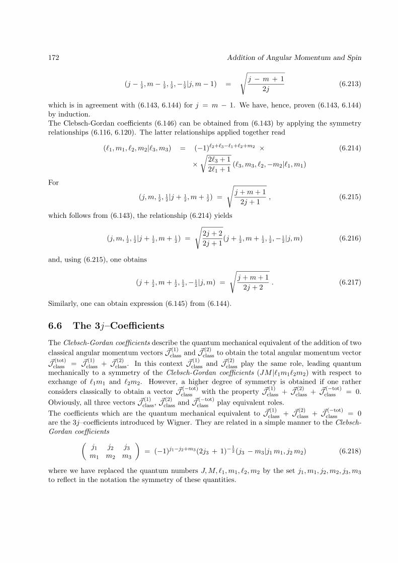
172 Addition of Angular Momentum and Spin
(j − 12,m− 1
2, 1
2,− 1
2|j,m− 1) =
√j − m + 1
2j(6.213)
which is in agreement with (6.143, 6.144) for j = m − 1. We have, hence, proven (6.143, 6.144)by induction.The Clebsch-Gordan coefficients (6.146) can be obtained from (6.143) by applying the symmetryrelationships (6.116, 6.120). The latter relationships applied together read
(`1,m1, `2,m2|`3,m3) = (−1)`2+`3−`1+`2+m2 × (6.214)
×√
2`3 + 12`1 + 1
(`3,m3, `2,−m2|`1,m1)
For
(j,m, 12, 1
2|j + 1
2,m+ 1
2) =
√j +m+ 1
2j + 1, (6.215)
which follows from (6.143), the relationship (6.214) yields
(j,m, 12, 1
2|j + 1
2,m+ 1
2) =
√2j + 22j + 1
(j + 12,m+ 1
2, 1
2,− 1
2|j,m) (6.216)
and, using (6.215), one obtains
(j + 12,m+ 1
2, 1
2,− 1
2|j,m) =
√j +m+ 1
2j + 2. (6.217)
Similarly, one can obtain expression (6.145) from (6.144).
6.6 The 3j–Coefficients
The Clebsch-Gordan coefficients describe the quantum mechanical equivalent of the addition of twoclassical angular momentum vectors ~J (1)
class and ~J (2)class to obtain the total angular momentum vector
~J (tot)class = ~J (1)
class + ~J (2)class. In this context ~J (1)
class and ~J (2)class play the same role, leading quantum
mechanically to a symmetry of the Clebsch-Gordan coefficients (JM |`1m1`2m2) with respect toexchange of `1m1 and `2m2. However, a higher degree of symmetry is obtained if one ratherconsiders classically to obtain a vector ~J (−tot)
class with the property ~J (1)class + ~J (2)
class + ~J (−tot)class = 0.
Obviously, all three vectors ~J (1)class, ~J
(2)class and ~J (−tot)
class play equivalent roles.The coefficients which are the quantum mechanical equivalent to ~J (1)
class + ~J (2)class + ~J (−tot)
class = 0are the 3j–coefficients introduced by Wigner. They are related in a simple manner to the Clebsch-Gordan coefficients(
j1 j2 j3m1 m2 m3
)= (−1)j1−j2+m3(2j3 + 1)−
12 (j3 −m3|j1m1, j2m2) (6.218)
where we have replaced the quantum numbers J,M, `1,m1, `2,m2 by the set j1,m1, j2,m2, j3,m3
to reflect in the notation the symmetry of these quantities.

6.6: The 3j–Coefficients 173
We first like to point out that conditions (6.21, 6.34) imply(j1 j2 j3m1 m2 m3
)= 0 if not m1 + m2 + m3 = 0 (6.219)(
j1 j2 j3m1 m2 m3
)= 0 if not |j1 − j2| ≤ j3 ≤ j1 + j2 . (6.220)
The latter condition |j1 − j2| ≤ j3 ≤ j1 + j2, the so-called triangle condition, states that j1, j2, j3form the sides of a triangle and the condition is symmetric in the three quantum numbers.According to the definition of the 3j–coefficients one would expect symmetry properties with respectto exchange of j1,m1, j2,m2 and j3,m3 and with respect to sign reversals of all three valuesm1,m2,m3, i.e. with respect to alltogether 12 symmetry operations. These symmetries follow theequations (
j1 j2 j3m1 m2 m3
)=(
j2 j3 j1m2 m3 m1
)= (−1)j1+j2+j3
(j2 j1 j3m2 m1 m3
)= (−1)j1+j2+j3
(j1 j2 j3−m1 −m2 −m3
)(6.221)
where the the results of a cyclic, anti-cyclic exchange and of a sign reversal are stated. In this waythe values of 12 3j-coefficients are related.However, there exist even further symmetry properties, discovered by Regge, for which no knownclassical analogue exists. To represent the full symmetry one expresses the 3j–coefficients througha 3× 3–matrix, the Regge-symbol, as follows(
j1 j2 j3m1 m2 m3
)=
−j1 + j2 + j3 j1 − j2 + j3 j1 + j2 − j3j1 −m1 j2 −m2 j3 −m3
j1 +m1 j2 +m2 j3 +m3
. (6.222)
The Regge symbol vanishes, except when all elements are non-negative integers and each row andcolumn has the same integer value Σ = j1 + j2 + j3. The Regge symbol also vanishes in case thattwo rows or columns are identical and Σ is an odd integer. The Regge symbol reflects a remarkabledegree of symmetry of the related 3j–coefficients: One can exchange rows, one can exchange columnsand one can reflect at the diagonal (transposition). In case of a non-cyclic exchange of rows andcolumns the 3j–coefficent assumes a prefactor (−1)Σ. These symmetry operations relate altogether72 3j–coefficients.The reader may note that the entries of the Regge-symbol, e.g., −j1 + j2 + j3, are identical to theinteger arguments which enter the analytical expression (6.102) of the Clebsch-Gordan coefficients,safe for the prefactor
√2j3 + 1 which is cancelled according to the definition (6.218) relating 3j-
coefficients and Clebsch-Gordan coefficients. The two integer entries J − `1 −m2 and J − `2 +m1
in (6.102) are obtained each through the difference of two entries of the Regge-symbol.Because of its high degree of symmetry the Regge symbol is very suited for numerical evaluationsof the 3j–coefficents. For this purpose one can use the symmetry transformations to place thesmallest element into the upper left corner of the Regge symbol. Assuming this placement theRegge symbol can be determined as follows (n11 is the smallest element!) n11 n12 n13
n21 n22 n23
n31 n32 n33
= (−1)n23+n32
√n12!n13!n21!n31!
(Σ + 1)!n11!n22!n33!n23!n32!))
n11∑n=0
sn (6.223)
174 Addition of Angular Momentum and Spin
where
Σ = n11 + n12 + n13 = j1 + j2 + j3 (6.224)s0 = n23!
(n23−n11)!n32!
(n32−n11)! (6.225)
sn = − (n11+1−n)(n22+1−n)(n33+1−n)n(n23−n11+n)(n32−n11+n) sn−1 . (6.226)
We like to state finally a few explicit analytical expressions for Clebsch-Gordan coefficients whichwere actually obtained using (6.223-6.226) by means of a symbolic manipulation package (Mathe-matica)
(1m|2m11m2) =(−1)1+m+m1 δ(m,m1 +m2)
√(2−m1)!
√(2 +m1)!
√10√
(1−m)!√
(1 +m)!√
(1−m2)!√
(1 +m2)!1 ≥ |m| ∧ 1 ≥ |m2| ∧ 2 ≥ |m1| (6.227)
(2m|2m11m2) =(−1)m+m1 (m+ 2m2) δ(m,m1 +m2)
√(2−m1)! (2 +m1)!
√6√
(2−m)!√
(2 +m)!√
(1−m2)!√
(1 +m2)!1 ≥ |m2| ∧ 2 ≥ |m| ∧ 2 ≥ |m1| (6.228)
(3m|2m11m2) =(−1)2m1−2m2
√7 δ(m,m1 +m2)
√(3−m)!
√(3 +m)!
√105√
(2−m1)!√
(2 +m1)!√
(1−m2)!√
(1 +m2)!1 ≥ |m2|) ∧ 2 ≥ |m1| ∧ 3 ≥ |m| (6.229)
(0m|12m1
12m2) =
i(−1)1−m2 δ(0,m) δ(−m1,m2)√2
12≥ |m1|) (6.230)
(1m|12m1
12m2) =
(−1)2m1−2m2√
3 δ(m,m1 +m2)√
(1−m)!√
(1 +m)!√
6√(
12 −m1
)!√(
12 +m1
)!√(
12 −m2
)!√(
12 +m2
)!
12≥ |m1| ∧
12≥ |m2| ∧ 1 ≥ |m| (6.231)
Here is an explicit value of a Clebsch-Gordan coefficient:
(7012 −151
2 |120−10 6012 −51
2) =4793185293503147294940209340
√127√
142√35834261990081573635135027068718971996984731222241334046198355
' 0.10752786393409395427444450130056540562826159542886 (6.232)
We also illustrate the numerical values of a sequence of 3j-coefficients in Figure 6.1.
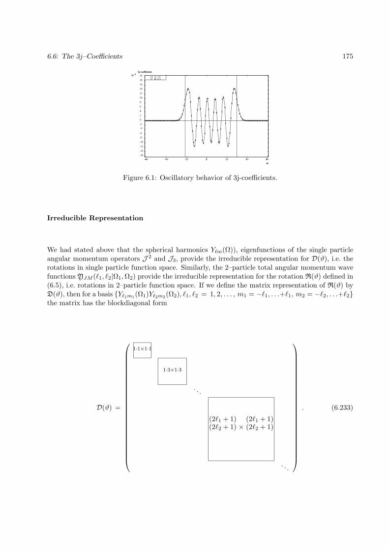
6.6: The 3j–Coefficients 175
-16
-14
-12
-10
-8
-6
-4
-2
0
2
46
8
10
12
14
16
18
20
-60 -40 -20 0 20 40 60
120 60 700-10 m 10-m
m
10 -33j coefficient
Figure 6.1: Oscillatory behavior of 3j-coefficients.
Irreducible Representation
We had stated above that the spherical harmonics Y`m(Ω)), eigenfunctions of the single particleangular momentum operators J 2 and J3, provide the irreducible representation for D(ϑ), i.e. therotations in single particle function space. Similarly, the 2–particle total angular momentum wavefunctions YJM (`1, `2|Ω1,Ω2) provide the irreducible representation for the rotation R(ϑ) defined in(6.5), i.e. rotations in 2–particle function space. If we define the matrix representation of R(ϑ) byD(ϑ), then for a basis Y`1m1(Ω1)Y`2m2(Ω2), `1, `2 = 1, 2, . . . , m1 = −`1, . . .+`1, m2 = −`2, . . .+`2the matrix has the blockdiagonal form
D(ϑ) =
1·1×1·1
1·3×1·3
. . .
(2`1 + 1)(2`2 + 1) ×
(2`1 + 1)(2`2 + 1)
. . .
. (6.233)

176 Addition of Angular Momentum and Spin
For the basis YJM (`1, `2|Ω1,Ω2), `1, `2 = 1, 2, . . . , J = |`1 − `2|, . . . , `1 + `2, M = −J, . . . Jeach of the blocks in (6.233) is further block-diagonalized as follows
(2`1 + 1)(2`2 + 1) ×
(2`1 + 1)(2`2 + 1) =
(2|`1 − `2|+ 1)×(2|`1 − `2|+ 1)
(2|`1 − `2|+ 3)×(2|`1 − `2|+ 3)
. . .
(2(`1 + `2) + 1)×(2(`1 + `2) + 1)
(6.234)
Partitioning in smaller blocks is not possible.
Exercise 6.6.1: Prove Eqs. (6.233,6.234)Exercise 6.6.2: How many overall singlet states can be constructed from four spin–1
2 states|12m1〉(1)|12m2〉(2)|12m3〉(3)|12m4〉(4)? Construct these singlet states in terms of the product wavefunctions above.Exercise 6.6.3: Two triplet states |1m1〉(1)|1m2〉(2) are coupled to an overall singlet state Y00(1, 1).Show that the probability of detecting a triplet substate |1m1〉(1) for arbitrary polarization (m2–value) of the other triplet is 1
3 .

6.7: Tensor Operators 177
6.7 Tensor Operators and Wigner-Eckart Theorem
In this Section we want to discuss operators which have the property that they impart angularmomentum and spin properties onto a quantum state. Such operators T can be characterizedthrough their behaviour under rotational transformations.Let T |ψ〉 denote the state obtained after the operator T has been applied and let R(~ϑ) denotea rotation in the representation of SO(3) or SU(2) which describes rotational transformationsof the quantum states under consideration, e.g. the operator (5.42) in case (i) of the positionrepresentation of single particle wave functions or the operator (5.222) in case (ii) of single particlespin operators. Note that in the examples mentioned the operator T would be defined within thesame representation as R(~ϑ). This implies, for example, that in
case (i) T is an operator C∞(3) → C∞(3) acting on single particle wave functions, e.g. a mul-tiplicative operator T ψ(~r) = f(~r)ψ(~r) or a differential operator T ψ(~r) = ( ∂2
∂x21
+ ∂2
∂x22
+∂2
∂x23)ψ(~r);
case (ii) the operator T could be a spin operator Sk defined in (5.223), e.g. S2 = S21 + S2
2 + S23
or any other polynomial of Sk.
The operator T may also act on multi-particle states like Y`1m1(r1)Y`2m2(r2). In fact, some of theexamples considered below involve tensor operators T of this type.Rotations transform |ψ〉 as |ψ′〉 = R(~ϑ)|ψ〉 and T |ψ〉 as R(~ϑ)T |ψ〉. The latter can be writtenT ′|ψ′〉 where T ′ denotes T in the rotated frame given by
T ′ = R(~ϑ)T R−1(~ϑ) . (6.235)
The property that T imparts onto states |ψ〉 angular momentum or spin corresponds to T behavingas an angular momentum or spin state multiplying |ψ〉. The latter implies that T transforms likean angular momentum or spin state |`m〉, i.e. that T belongs to a family of operators Tkq, q =−k,−k + 1, . . . k such that
T ′kq =k∑
q′=−kD(k)q′q (~ϑ)Tkq′ . (6.236)
In this equation D(k)q′q (~ϑ) denotes the rotation matrix
D(k)q′q (~ϑ) = 〈kq′|R(~ϑ)|kq〉 . (6.237)
The operators T ∈ Tkq, q = −k,−k + 1, . . . k with the transformation property (6.236, 6.237)are called tensor operators of rank k.
Examples of Tensor Operators
The multiplicative operators C∞(3) → C∞(3)
Ykq(~r) def= rkYkq(r) (6.238)

178 Theory of Angular Momentum and Spin
are tensor operators of rank k. Examples are
Y00 =1√4π
Y1±1 = ∓√
38πr sinθ e±iφ = ∓
√3
8π(x1 ± ix2)
Y10 =
√3
4πr cosθ =
√3
4πx3
Y2±2 =14
√152πr2 sin2θ e±2iφ =
14
√152π
(x1 ± ix2)2
Y2±1 = ∓√
158πr2 sinθ e±iφ = ∓
√158π
(x1 ± ix2)x3
Y20 =
√5
4πr2
(32
cos2θ − 12
)=
√5
4π
(32x2
3 −r2
2
)(6.239)
These operators can be expressed in terms of the coordinates x1, x2, x3. The fact that these opera-tors form tensor operators of rank 1, 2, 3 follows from the transformation properties of the sphericalharmonics derived in Section 1.3.
Exercise 6.7.1: Show that the following set of spin operators
T00 = 1
T1±1 = ∓ 1√2S±
T10 = S3
T2±2 =(S±)2
T2±1 = ∓(S3S± + S±S3)
T20 =
√23
(3S23 − S2)
are tensor operators of rank 0, 1, 2.Exercise 6.7.2: Express the transformed versions of the following operators (a) T = x2
1 − x22 and
(b) S2S3 in terms of Wigner rotation matrices and untransformed operators.
For the following it is important to note that the rotation matrix elements (6.237) do not requirethat the rotation R−1(~ϑ) is expressed in terms of Euler angles according to (5.203), but ratherany rotation and any parametrization can be assumed. In fact, we will assume presently that therotation is chosen as follows
R(~ϑ) = exp (ϑ+L+ + ϑ−L− + ϑ3L3 ) (6.240)
where we have defined ϑ± = 12(ϑ1 ∓ iϑ2) and L± = L1 ± iL2. This choice of parametrization
allows us to derive conditions which are equivalent to the property (6.235 - 6.237), but are far easierto ascertain for any particular operator.
6.7: Tensor Operators 179
The conditions can be derived if we consider the property (6.235 - 6.237) for transformationscharacterized by infinitesimal values of ϑ+, ϑ−, ϑ3. We first consider a rotation with ~ϑ = (ϑ+, 0, 0)T
in case of small ϑ+. The property (6.235 - 6.237) yields first
R(~ϑ)TkqR−1(~ϑ) =k∑
q′=−k〈kq′|R(~ϑ)|kq〉Tkq′ . (6.241)
Using R(~ϑ) = 11 + ϑ+L+ + O(ϑ2+) this equation can be rewritten neglecting terms of order O(ϑ2
+)
(11 + ϑ+L+)Tkq (11 − ϑ+L+) =k∑
q′=−k〈kq′|11 + ϑ+L+|kq〉Tkq′ . (6.242)
from which follows by means of 〈kq′|11|kq〉 = δqq′ and by subtracting Tkq on both sides of theequation
ϑ+ [L+, Tkq] =k∑
q′=−kϑ+〈kq′|L+|kq〉Tkq′ . (6.243)
From (5.80) follows 〈kq′|L+|kq〉 = −i√
(k + q + 1)(k − q)δq′ q+1 and, hence,
[L+, Tkq] = −iTk q+1
√(k + q + 1)(k − q) . (6.244)
Similar equations can be derived for infinitesimal rotations of the form ~ϑ = (0, ϑ−, 0)T , (0, 0, ϑ3)T .Expressing the results in terms of the angular momentum operators J+, J−, J3 yields
[J+, Tkq] = ~Tkq+1
√(k + q + 1)(k − q) (6.245)
[J−, Tkq] = ~Tkq−1
√(k + q)(k − q + 1) (6.246)
[J3, Tkq] = ~ q Tkq . (6.247)
These properties often can be readily demonstrated for operators and the transformation properties(6.235 - 6.237) be assumed then.
Exercise 6.7.3: Derive Eqs. (6.246, 6.247).Exercise 6.7.4: Is the 1-particle Hamiltonian
H = − ~2
2m∇2 + V (|~r|) (6.248)
a tensor operator?Exercise 6.7.5: Consider a system of two spin-1
2 particles for which the first spin is described bythe operator ~S(1) and the second spin by the operator ~S(2). Show that ~S(1) · ~S(2) is a tensor operatorof rank 0 in the space of the products of the corresponding spin states |12m1〉(1)|12m2〉(2). For thispurpose state first the proper rotation operator R(~ϑ) and note then that ~S(1) · ~S(2) commutes withthe generators of the rotation of |12m1〉(1)|12m2〉(2).Exercise 6.7.6: Form tensor operators of rank 1 in terms of the three components of ∇ acting onthe space of 1-particle wave functions.

180 Theory of Angular Momentum and Spin
6.8 Wigner-Eckart Theorem
A second important property of tensor operators Tkq beside (6.235 - 6.237) is that their matrix ele-ments 〈`1m1γ1|Tkq|`2m2γ2〉 obey simple relationships expressed in terms of Clebsch-Gordan coeffi-cients. |`1m1γ1〉 denotes an angular momentum (spin) state, possibly the total angular momentum–spin state of a compositie system, which is characterized also by a set of other quantum numbers γ1
which are not affected by the rotational transformation R(~ϑ). The relationships among the matrixelements 〈`1m1γ1|Tkq|`2m2γ2〉 are stated by the Wigner–Eckart theorem which we will derive now.Starting point of the derivation is the fact that the states Tkq|`2m2γ2〉 behave like angular momen-tum states of a composite system of two particles each carrying angular momentum or spin, i.e.behave like |kq〉|`1m1〉. To prove this we consider the transformation of Tkq|`2m2γ2〉
R(~ϑ)Tkq |`2m2γ2〉 = R(~ϑ)TkqR−1(~ϑ)R(~ϑ) |`2m2γ2〉
=∑q′m′2
D(k)q′qTkq′ D
(`2)m′2m2
|`2m′2γ2〉 (6.249)
which demonstrates, in fact, the stated property. One can, hence, construct states Φ`1m1(k, `2|γ2)which correspond to total angular momentum states. These states according to (6.18) are definedthrough
Φ`1m1(k, `2|γ2) =∑q,m2
(`1m1|kq `2m2)Tkq |`2m2γ2〉 . (6.250)
We want to show now that these states are eigenstates of J2 = J21 + J2
2 + J23 and of J3 where
J1, J2, J3 are the generators of the rotation R(~ϑ). Before we proceed we like to point out that thestates |`2m2γ2〉 are also eigenstates of J2, J3, i.e.
J2 |`2m2γ2〉 = ~2`2(`2 + 1) |`2m2γ2〉 ; J3 |`2m2γ2〉 = ~m2 |`2m2γ2〉 . (6.251)
The corresponding property for Φ`1m1(k, `2|γ2) can be shown readily as follows using (6.247),J3|`2m2γ2〉 = ~m2γ2|`2m2〉 and the property (6.21) of Clebsch-Gordan coefficients
J3 Φ`1m1(k, `2|γ2) =∑q,m2
(`1m1|kq `2m2) (J3Tkq − TkqJ3︸ ︷︷ ︸=~qTkq
+TkqJ3) |`2m2γ2〉
= ~
∑q,m2
(`1m1|kq `2m2)︸ ︷︷ ︸∼δm1 q+m2
(q + m2)Tkq |`2m2γ2〉
= ~m1
∑q,m2
(`1m1|kq `2m2)Tkq |`2m2γ2〉 (6.252)
Similarly, one can show that Φ`1m1(k, `2|γ2) is an eigenstate of J2 with eigenvalue ~2`1(`1 +1). Thehermitian property of J3 and J2 implies that states Φ`1m1(k, `2|γ2) are orthogonal to |`′1m′1〉 in caseof different quantum numbers `1,m1, i.e.
〈`′1m′1|Φ`1m1(k, `2|γ2) = C δ`1`′1δm1m′1(6.253)
Exercise 6.8.1: Show that Φ`1m1(k, `2|γ2) is an eigenstate of J2 with eigenvalue ~2`1(`1 + 1).

6.8: Wigner-Eckart Theorem 181
In order to evaluate the matrix elements 〈`1m1γ1|Tkq|`2m2γ2〉 we express using the equivalent of(6.32)
Tkq |`2m2γ2〉 =∑`1m1
(`1m1|kq`2m2) Φ`1m1(k`2|γ2) (6.254)
and orthogonality property (6.253)
〈`1m1γ1|Tkq|`2m2γ2〉 = 〈`1m1γ1|Φ`1m1(k`2|γ2)〉 (`1m1|kq`2m2) . (6.255)
At this point the important property can be proven that 〈`1m1γ1|Φ`1m1(k`2|γ2)〉 is independentof m1, i.e. the matrix elements 〈`1m1γ1|Tkq|`2m2γ2〉 can be reduced to an m1–independent factor,its m1–dependence being expressed solely through a Clebsch-Gordan coefficient. To prove thisproperty we consider 〈`1m1γ1|Φ`1m1(k`2|γ2)〉 for a different m1 value, say m1 + 1. Using
|`1m1 + 1γ1〉 =1√
(`1 +m1 + 1)(`1 −m1)J+|`1m1γ1〉 (6.256)
and noting that the operator adjoint to J+ is J−, one obtains
〈`1m1 + 1γ1|Φ`1m1+1(k`2|γ2) =1√
(`1+m1+1)(`1−m1)〈`1m1γ1|J−Φ`1m1+1(k`2|γ2)〉 =
〈`1m1γ1|Φ`1m1(k`2|γ2)〉 (6.257)
which establishes the m1–independence of 〈`1m1γ1|Φ`1m1(k`2|γ2)〉. In order to express the m1–independence explicitly we adopt the following notation
〈`1m1γ1|Φ`1m1(k`2|γ2)〉 = (−1)k−`2+`1 1√2`1 + 1
〈`1, γ1||Tk||`2, γ2〉 . (6.258)
We can then finally express the matrix elements of the tensor operators Tkq as follows
〈`1m1, γ1|Tkq|`2m2, γ2〉 =(`1m1|kq`2m2) (−1)k−`2+`1 1√
2`1+1〈`1, γ1||Tk||`2, γ2〉 (6.259)
The socalled reduced matrix element 〈`1, γ1||Tk||`2, γ2〉 is determined by applying (6.259) to acombination of magnetic quantum numbers m′1, q
′,m′2, e.g. m′1 = q′ = m′2 = 0, for whichthe l.h.s. can be evaluated as easily as possible. One can then evaluate also the correspondingClebsch-Gordan coefficient (`1m′1|kq′`2m′2) and determine
〈`1, γ1||Tk||`2, γ2〉 =√
2`1 + 1〈`1m′1, γ1|Tkq′ |`2m′2, γ2〉
(−1)k−`2+`1(`1m′1|kq′`2m′2)(6.260)
Exercise 6.8.2: Determine the matrix elements of the gradient operator ∇ of the type∫d3rF (~r)∇G(~r) (6.261)

182 Theory of Angular Momentum and Spin
when the functions F (~r) and G(~r) are of the type f(r)Y`m(r). For this purpose relate ∇ to a tensoroperator T1q, evaluate the matrix for m1 = q = m2 = 0 using
cosθ Y`m(θ, φ) =√(`+1−m)(`+1+m)
(2`+1)(2`+3) Y`+1m(θ, φ) +√
(`−m)(`+m)(2`−1)(2`+1) Y`−1m(θ, φ)
sinθ Y`m(θ, φ) =`(`+1)√
(2`+1)(2`+3)Y`+1m(θ, φ) − `(`−1)√
2`−1)(2`+1)Y`−1m(θ, φ)
and express the remaining matrix elements using the Wigner–Eckart theorem. (The necessaryevaluations are cumbersome, but a very useful exercise!)
Chapter 7
Motion in Spherically SymmetricPotentials
We describe in this section the stationary bound states of quantum mechanical particles in spher-ically symmetric potentials V (r), i.e., in potentials which are solely a function of r and are inde-pendent of the angles θ, φ. Four examples will be studied. The first potential
V (r) =
0 0 ≤ r ≤ R∞ r > R
(7.1)
confines a freely moving particle to a spherical box of radius R. The second potential is of thesquare well type
V (r) =−Vo 0 ≤ r ≤ R0 r > R
. (7.2)
The third potential
V (r) =12mω2r2 (7.3)
describes an isotropic harmonic oscillator . The fourth potential
V (r) = − Z e2
r(7.4)
governs the motion of electrons in hydrogen-type atoms.Potential (7.4) is by far the most relevant of the four choices. It leads to the stationary electronicstates of the hydrogen atom (Z = 1). The corresponding wave functions serve basis functions formulti-electron systems in atoms, molecules, and crystals. The potential (7.3) describes the motionof a charge in a uniformely charged sphere and can be employed to describe the motion of protonsand neutrons in atomic nuclei1. The potentials (7.1, 7.2) serve as schematic descriptions of quantumparticles, for example, in case of the so-called bag model of hadronic matter.
1See, for example, Simple Models of Complex Nuclei / The Shell Model and the Interacting Boson Model by I.Talmi (Harwood Academic Publishers, Poststrasse 22, 7000 Chur, Switzerland, 1993)
183
184 Spherically Symmetric Potentials
7.1 Radial Schrodinger Equation
A classical particle moving in a potential V (r) is governed by the Newtonian equation of motion
m~v = − er ∂rV (r) . (7.5)
In the case of an angular independent potential angular momentum ~J = m~r × ~v is a constant ofmotion. In fact, the time variation of ~J can be written, using (7.5) and ~r = ~v,
d
dt~J = ~v ×m~v + ~r ×m~v = 0 + ~r × er (−∂rV (r)) = 0 . (7.6)
Since Jk is also equal to the poisson bracket H,Jk where H is the Hamiltonian, one can conclude
Jk = H,Jk = 0 , k = 1, 2, 3. (7.7)
The correspondence principle dictates then for the quantum mechanical Hamiltonian operator Hand angular momentum operators Jk
[H, Jk] = 0 , k = 1, 2, 3 . (7.8)
This property can also be proven readily employing the expression of the kinetic energy operator[c.f. (5.99)]
− ~2
2m∇2 = − ~
2
2m1r∂2r r +
J 2
2mr2, (7.9)
the expressions (5.85– 5.87) for Jk as well as the commutation property (5.61) of J 2 and Jk. Ac-cordingly, stationary states ψE,`,m(~r) can be chosen as simultaneous eigenstates of the Hamiltonianoperator H as well as of J 2 and J3, i.e.,
H ψE,`,m(~r) = E ψE,`,m(~r) (7.10)J 2ψE,`,m(~r) = ~
2`(`+ 1)ψE,`,m(~r) (7.11)J3ψE,`,m(~r) = ~mψE,`,m(~r) . (7.12)
In classical mechanics one can exploit the conservation of angular momentum to reduce the equationof motion to an equation governing solely the radial coordinate of the particle. For this purposeone concludes first that the conservation of angular momentum ~J implies a motion of the particleconfined to a plane. Employing in this plane the coordinates r, θ for the distance from the originand for the angular position, one can state
J = mr2 θ . (7.13)
The expression of the kinetic energy
~p 2
2m=
12m r2 +
12mr2θ2 =
12m r2 +
J2
2mr2(7.14)
and conservation of energy yield
12m r2 +
J2
2mr2+ V (r) = E . (7.15)
7.1: Radial Schrodinger Equation 185
This is a differential equation which governs solely the radial coordinate. It can be solved byintegration of
r = ±
2m
[E − V (r) − J2
2mr2
] 12
. (7.16)
Once, r(t) is determined the angular motion follows from (7.13), i.e., by integration of
θ =J
mr2(t). (7.17)
In analogy to the classical description one can derivem, in the present case, for the wave functionof a quantum mechanical particle a differential equation which governs solely the r-dependence.Employing the kinetic energy operator in the form (7.9) one can write the stationary Schrodingerequation (7.10), using (7.11),[
− ~2
2m1r∂2r r +
J 2
2mr2+ V (r) − E`,m
]ψE,`,m(~r) = 0 . (7.18)
Adopting for ψE,`,m(~r) the functional form
ψE,`,m(~r) = vE,`,m(r)Y`m(θ, φ) (7.19)
where Y`m(θ, φ) are the angular momentum eigenstates defined in Section 5.4, equations (7.11, 7.12)are obeyed and one obtains for (7.10)[
− ~2
2m1r∂2r r +
~2`(`+ 1)2mr2
+ V (r) − E`,m
]vE,`,m(r) = 0 . (7.20)
Since this equation is independent of the quantum number m we drop the index m on the radialwave function vE,`,m(r) and E`,m.One can write (7.20) in the form of the one-dimensional Schrodinger equation[
− ~2
2m∂2r + Veff(r) − E
]φE(r) = 0 . (7.21)
where
Veff(r) = V (r) +~
2`(`+ 1)2mr2
(7.22)
φE(r) = r vE,`,m(r) . (7.23)
This demonstrates that the function r vE,`,m(r) describes the radial motion as a one-dimensionalmotion in the interval [0, ∞[ governed by the effective potential (7.22) which is the original potentialV (r) with an added rotational barrier potential ~
2`(`+1)2mr2 . This barrier, together with the original
potential, can exclude particles from the space with small r values, but can also trap particles inthe latter space giving rise to strong scattering resonances (see Section ??).Multiplying (7.20) by −2mr/~2 yields the so-called radial Schrodinger equation[
∂2r −
`(`+ 1)r2
− U(r) − κ2`
]r vκ,`(r) = 0 . (7.24)

186 Spherically Symmetric Potentials
where we defined
U(r) = −2m~
2V (r) (7.25)
κ2` = −2m
~2E` (7.26)
In case E < 0, κ assumes real values. We replaced in (7.20) the index E by the equivalent indexκ.
Boundary Conditions
In order to solve (7.20) one needs to specify proper boundary conditions2. For r → 0 one mayassume that the term `(`+ 1)/r2 becomes larger than the potential U(r). In this case the solutionis governed my [
∂2r −
`(`+ 1)r2
]r vκ,`(r) = 0 , r → 0 (7.27)
and, accordingly, assumes the general form
r vκ,`(r) ∼ Ar`+1 + B r−` (7.28)
orvκ,`(r) ∼ Ar` + B r−`−1 (7.29)
Only the first term is admissable. This follows for ` > 0 from consideration of the integral whichmeasures the total particle density. The radial part of this integral is∫ ∞
0dr r2 v2
κ,`(r) (7.30)
and, hence, the term Br−(`+1) would contribute
|B|2∫ ε
0dr r−2` (7.31)
which, for ` > 0 is not integrable. For ` = 0 the contribution of Br−(`+1) to the complete wavefunction is, using the expression (5.182) for Y00,
ψE,`,m(~r) ∼ B√4π|~r|
. (7.32)
The total kinetic energy resulting from this contribution is, according to a well-known result inClassical Electromagnetism3,
~2
2m∇2ψE,`,m(~r) ∼
√4π B δ(x1)δ(x2)δ(x3) . (7.33)
2A detailed discussion of the proper boundary conditions, in particular, at r = 0 is found in the excellentmonographs Quantum Mechanics I, II by A. Galindo and P. Pascual (Springer, Berlin, 1990)
3We refer here to the fact that the function Φ(~r) = 1/r is the solution of the Poisson equation ∇2 =−4πδ(x)δ(y)δ(z); see, for example, ”Classical Electrodynamics, 2nd Ed.” by J.D. Jackson (John Wiley, New York,1975).

7.1: Radial Schrodinger Equation 187
Since there is no term in the stationary Schrodinger equation which could compensate this δ-function contribution we need to postulate that the second term in (7.29) is not permissible. Onecan conclude that the solution of the radial Schrodinger equation must obey
r vκ,`(r) → 0 for r → 0 . (7.34)
The boundary conditions for r → ∞ are governed by two terms in the radial Schrodinger equation,namely, [
∂2r − κ2
`
]r vκ,`(r) = 0 for r → ∞ . (7.35)
We have assumed here limr→∞ V (r) = 0 which is the convention for potentials. The solution ofthis equation is
r vκ,`(r) ∼ Ae−κr + B e+κr for r → ∞ . (7.36)
For bound states κ is real and, hence, the second contribution is not permissible. We conclude,therefore, that the asymptotic boundary condition for the solution of the radial Schrodinger equa-tion (7.20) is
r vκ,`(r) ∼ e−κr for r → ∞ . (7.37)
Degeneracy of Energy Eigenvalues
We have noted above that the differential operator appearing on the l.h.s. of the in radialSchrodinger equation (7.24) is independent of the angular momentum quantum number m. Thisimplies that the energy eigenvalues associated with stationary bound states of radially symmetricpotentials with identical `, but different m quantum number, assume the same values. This be-haviour is associated with the fact that any rotational transformation of a stationary state leavesthe energy of a stationary state unaltered. This property holds since (7.8) implies
[H, exp(− i~
ϑ · ~J ) ] = 0 . (7.38)
Applying the rotational transformation exp(− i~ϑ · ~J ) to (7.10) yields then
H exp(− i~
ϑ · ~J )ψE,`,m(~r) = E exp(− i~
ϑ · ~J )ψE,`,m(~r) , (7.39)
i.e., any rotational transformation produces energetically degenerate stationary states. One mightalso apply the operators J± = J1 ± iJ2 to (7.10) and obtain for −` < m < `
H J± ψE,`,m(~r) = E J± ψE,`,m(~r) , (7.40)
which, together with the identities (5.172, 5.173), yields
H ψE,`,m±1(~r) = E ψE,`,m±1(~r) (7.41)
where E is the same eigenvalue as in (7.40). One expect, therefore, that the stationary states forspherically symmetric potentials form groups of 2` + 1 energetically degenerate states, so-calledmultiplets where ` = 0, 1, 2, . . .. Following a convention from atomic spectroscopy, one refers tothe multiplets with ` = 0, 1, 2, 3 as the s, p, d, f -multipltes, respectively.In the remainder of this section we will solve the radial Schrodinger equation (7.20) for the potentialsstated in (7.1–7.4). We seek to describe bound states for the particles, i.e., states with E < 0.States with E > 0, which play a key role in scattering processes, will be described in Section ??.

188 Spherically Symmetric Potentials
7.2 Free Particle Described in Spherical Coordinates
We consider first the case of a particle moving in a force-free space described by the potential
V (r) ≡ 0 . (7.42)
The stationary Schrodinger equation for this potential reads[− ~
2
2m∇2 − E
]ψE(~r) = 0 . (7.43)
Stationary States Expressed in Cartesian Coordinates The general solution of (7.43), asexpressed in (3.74–3.77), is
ψ(~k|~r) = N ei~k·~r (7.44)
where
E =~
2k2
2m≥ 0 . (7.45)
The possible energies can assume continuous values. N in (7.44) is some suitably chosen normal-ization constant; the reader should be aware that (7.44) does not represent a localized particle andthat the function is not square integrable. One chooses N such that the orthonormality property∫
Ω∞
d3r ψ∗(~k ′|~r)ψ(~k|~r) = δ(~k ′ − ~k) (7.46)
holds. The proper normalization constant is N = (2π)−3/2.In case of a force-free motion momentum is conserved. In fact, the Hamiltonian in the present case
Ho = − ~2
2m∇2 (7.47)
commutes with the momentum operator ~p = (~/i)∇ and, accordingly, the eigenfunctions of (7.45)can be chosen as simultaneous eigenfunction of the momentum operator. In fact, it holds
~pN ei~k·~r = ~~k N ei
~k·~r . (7.48)
as one can derive using in (7.48) Cartesian coordinates, i.e.,
∇ =
∂1
∂2
∂3
, ~k · ~r = k1x1 + k2x2 + k3x3 . (7.49)
Stationary States Expressed in Spherical Coordinates Rather than specifying energythrough k = |~k| and the direction of the momentum through k = ~k/|~k| one can exploit thefact that the angular momentum operators J 2 and J3 given in (5.97) and in (5.92), respectively,commute with Ho as defined in (7.47). This latter property follows from (5.100) and (5.61). Ac-cordingly, one can choose stationary states of the free particle which are eigenfunctions of (7.47) aswell as eigenfunctions of J 2 and J3 described in Sect. 5.4.
7.2: Free Particle 189
The corresponding stationary states, i.e., solutions of (7.43) are given by wave functions of the form
ψ(k, `,m|~r) = vk,`(r)Y`m(θ, φ) (7.50)
where the radial wave functions obeys [c.f. (7.20)][− ~
2
2m1r∂2r r +
~2`(`+ 1)2mr2
− E`,m
]vk,`(r) = 0 . (7.51)
Using (7.45) and multiplying (7.20) by −2mr/~2 yields the radial Schrodinger equation[∂2r −
`(`+ 1)r2
+ k2
]r vk,`(r) = 0 . (7.52)
We want to determine now the solutions vk,`(r) of this equation.We first notice that the solution of (7.52) is actually only a function of kr, i.e., one can writevk,`(r) = j`(kr). In fact, one can readily show, introducing the new variable z = kr, that (7.52)is equivalent to [
d2
dz2− `(`+ 1)
z2+ 1
]z j`(z) = 0 . (7.53)
According to the discussion in Sect. 7.1 the regular solution of this equation, at small r, behaveslike
j`(z) ∼ z` for r → 0 . (7.54)
There exists also a so-called irregular solution of (7.53), denoted by n`(z) which behaves like
n`(z) ∼ z−`−1 for r → 0 . (7.55)
We will discuss further below also this solution, which near r = 0 is inadmissable in a quantummechanical wave function, but admissable for r 6= 0.For large z values the solution of (7.53) is governed by[
d2
dz2+ 1
]z j`(z) = 0 for r → ∞ (7.56)
the general solution of which is
j`(z) ∼1z
sin(z + α) for r → ∞ (7.57)
for some phase α.We note in passing that the functions g`(z) = j`(z), n`(z) obey the differential equation equivalentto (7.53) [
d2
dz2+
2z
d
dz− `(`+ 1)
z2+ 1
]g`(z) = 0 . (7.58)
Noting that sin(z + α) can be written as an infinite power series in z we attempt to express thesolution of (7.53) for arbitary z values in the form
j`(z) = z` f(z2) , f(z2) =∞∑n=0
an z2n . (7.59)

190 Spherically Symmetric Potentials
The unknown expansion coefficients can be obtained by inserting this series into (7.53). We haveintroduced here the assumption that the factor f in (7.59) depends on z2. This follows from
d2
dz2z`+1f(z) = z`+1 d2
dz2f(z) + 2(`+ 1)z`
d
dzf + `(`+ 1)z`−1f (7.60)
from which we can conclude(d2
dz2+ (`+ 1)
2z
d
dz+ 1
)f(z) = 0 . (7.61)
Introducing the new variable v = z2 yields, using
1z
d
dz= 2
d
dv,
d2
dz2= 4v
d2
dv2+ 2
d
dv, (7.62)
the differential equation (d2
dv2+
2`+ 32v
d
dv+
14v
)f(v) = 0 (7.63)
which is consistent with the functional form in (7.59). The coefficients in the series expansion off(z2) can be obtained from inserting
∑∞n=0 an z
2n into (7.63) (v = z2)∑n
(an n (n− 1) vn−2 +
12
(2`+ 3) an vn−2 +14an v
n−1
)= 0 (7.64)
Changing the summation indices for the first two terms in the sum yields∑n
(an+1 n (n− 1) +
12
(2`+ 3) an +14an
)vn−1 = 0 . (7.65)
In this expression each term ∼ vn−1 must vanish individually and, hence,
an+1 = −12
1(n+ 1) (2n + 2` + 3)
an (7.66)
One can readily derive
a1 = −12
11! (2`+ 3)
a0 , a2 =14
12! (2`+ 3)(2`+ 5)
a0 . (7.67)
The common factor a0 is arbitrary. Choosing
a0 =1
1 · 3 · 5 · (2`+ 1). (7.68)
the ensuing functions (` = 0, 1, 2, . . .)
j`(z) =z`
1 · 3 · 5 · · · (2`+ 1)
[1 −
12z
2
1!(2`+ 3)+
(12z
2)2
2!(2`+ 3)(2`+ 5)− + · · ·
](7.69)
are called regular spherical Bessel functions.

7.2: Free Particle 191
One can derive similarly for the solution (7.55) the series expansion (` = 0, 1, 2, . . .)
n`(z) = − 1 · 3 · 5 · · · (2`− 1)z`+1
[1 −
12z
2
1!(1− 2`)+
(12z
2)2
2!(1− 2`)(3− 2`)− + · · ·
]. (7.70)
These functions are called irregular spherical Bessel functions.
Exercise 7.2.1: Demonstrate that (7.70) is a solution of (7.52) obeying (7.55).
The Bessel functions (7.69, 7.70) can be expressed through an infinite sum which we want to specifynow. For this purpose we write (7.69)
j`(z) =(z
2
)` 112 ·
32 ·
52 · · · (`+ 1
2)[1 +
((iz2
)21!(`+ 3
2)+
(((iz2
)42!(`+ 3
2)(2`+ 52)
+ · · ·
](7.71)
The factorial-type products12· 3
2· · ·(`+
12
)(7.72)
can be expressed through the so-called Gamma-function4 defined through
Γ(z) =∫ ∞
0dt tz−1 e−t . (7.73)
This function has the following properties5
Γ(z + 1) = z Γ(z) (7.74)Γ(n+ 1) = n! for n ∈ N (7.75)
Γ( 12) =
√π (7.76)
Γ(z) Γ(1− z) =π
sinπz. (7.77)
from which one can deduce readily
Γ(`+ 12) =
√π · 1
2· 3
2· · ·(`+
12
). (7.78)
One can write then
j`(z) =√π
2
(z2
)` ∞∑n=0
(iz2
)2nn! Γ(n+ 1 + `+ 1
2). (7.79)
4For further details see Handbook of Mathematical Functions by M. Abramowitz and I.A. Stegun (Dover Publica-tions, New York)
5The proof of (7.74–7.76) is elementary; a derivation of (7.77) can be found in Special Functions of MathematicalPhysics by A.F. Nikiforov and V.B. Uvarov, Birkhauser, Boston, 1988)
192 Spherically Symmetric Potentials
Similarly, one can express n`(z) as given in (7.70)
n`(z) = − 2`√πz`+1
Γ(`+12
)
[1 +
(iz2
)21!(1
2 − `)+
(iz2
)42!(1
2 − `)(32 − `)
+ · · ·
]. (7.80)
Using (7.77) for z = `+ 12 , i.e.,
Γ(`+ 12) = (−1)`
π
Γ(12 − `)
(7.81)
yields
n`(z) = (−1)`+1√π 2`
z`+1
[1
Γ(12 − `)
+
(iz2
)21! Γ(1
2 − `)(12 − `)
+
(iz2
)42! Γ(1
2 − `)(12 − `)(
32 − `)
+ · · ·
]. (7.82)
or
n`(z) = (−1)`+1
√π
2
(2z
)`+1 ∞∑n=0
(iz2
)2nn! Γ(n+ 1− `− 1
2). (7.83)
Linear independence of the Regular and Irregular spherical Bessel Functions
We want to demonstrate now that the solutions (7.69) and (7.69) of (7.53) are linearly independent.For this purpose we need to demonstrate that the Wronskian
W (j`, n`) = j`(z)d
dzn` −
d
dzj`(z)n` (7.84)
does not vanish. Let f1, f2 be solutions of (7.53), or equivalently, of (7.58). Using
d2
dz2f1,2 = − 2
z
d
dzf1,2 +
`(`+ 1)z2
f1,2 − f1,2 (7.85)
one can demonstrate the identity
d
dzW (f1, f2) = −2
zW (f1, f2) (7.86)
This equation is equivalent tod
dzlnW =
d
dzln
1z2
(7.87)
the solution of which islnW =
c
z2(7.88)
for some constant c. For the case of f1 = j` and f2 = n` this constant can be determined usingthe expansions (7.69, 7.70) keeping only the leading terms. One obtains c = 1 and, hence,
W (j`, n`) =1z2
. (7.89)
The Wronskian (7.89) doesn not vanish and, therefore, the regular and irregular Bessel functionsare linearly independent.

7.2: Free Particle 193
Relationship to Bessel functions
The differential equation (7.58) for the spherical Bessel functions g`(z) can be simplified by seekingthe corresponding equation for G`+ 1
2(z) defined through
g`(z) =1√zG`+ 1
2(z). (7.90)
Using
d
dzg`(z) =
1√z
d
dzG`+ 1
2(z) − 1
2z√zG`+ 1
2(z) (7.91)
d2
dz2g`(z) =
1√z
d2
dz2G`+ 1
2(z) − 1
z√z
d
dzG`+ 1
2(z) +
34z2√zG`+ 1
2(z)
(7.92)
one is lead to Bessel’s equation[d2
dz2+
1z
d
dz− ν2
z2+ 1
]Gν(z) = 0 (7.93)
where ν = ` + 12 . The regular solution of this equation is called the regular Bessel function. Its
power expansion, using the conventional normalization, is given by [c.f. (7.79)]
Jν(z) =(z
2
)ν ∞∑n=0
(iz/2)2n
n! Γ(ν + n+ 1). (7.94)
One can show that J−ν(z), defined through (7.94), is also a solution of (7.93). This follows fromthe fact that ν appears in (7.93) only in the form ν2. In the present case we consider solely thecase ν = ` + 1
2 . In this case J−ν(z) is linearly independent of Jν(z) since the Wronskian
W (J`+ 12, J−`− 1
2) = (−1)`
2πz
(7.95)
is non-vanishing. One can relate J`+ 12
and J−`− 12
to the regular and irregular spherical Besselfunctions. Comparision with (7.79) and (7.83) shows
j`(z) =√
π
2zJ`+ 1
2(z) (7.96)
n`(z) = (−1)`+1
√π
2zJ−`− 1
2(z) . (7.97)
These relationships are employed in case that since numerical algorithms provide the Bessel func-tions Jν(z), but not directly the spherical Bessel functions j`(z) and n`(z).
Exercise 7.2.2: Demonstrate that expansion (7.94) is indeed a regular solution of (7.93). Adoptthe procedures employed for the function j`(z).Exercise 7.2.3: Prove the identity (7.95).

194 Spherically Symmetric Potentials
Generating Function of Spherical Bessel Functions
The stationary Schrodinger equation of free particles (7.43) has two solutions, namely, one givenby (7.44, 7.45) and one given by (7.50). One can expand the former solution in terms of solutions(7.50). For example, in case of a free particle moving along the x3-axis one expands
eik3x3 =∑`,m
a`m j`(kr)Y`m(θ, φ) . (7.98)
The l.h.s. can be written exp(ikr cos θ), i.e., the wave function does not depend on φ. In this casethe expansion on the r.h.s. of (7.98) does not involve any non-vanishing m-values since Y`m(θ, φ)for non-vanishing m has a non-trivial φ-dependence as described by (5.106). Since the sphericalharmonics Y`0(θ, φ), according to (5.178) are given in terms of Legendre polynomials P`(cos θ) onecan replace the expansion in (7.98) by
eik3x3 =∞∑`=0
b` j`(kr)P`(cos θ) . (7.99)
We want to determine the expansion coefficients b`.The orthogonality properties (5.179) yield from (7.99)∫ +1
−1d cos θ eikr cos θ P`(cos θ) = b` j`(kr)
22` + 1
. (7.100)
Defining x = cos θ, z = kr, and using the Rodrigues formula for Legendre polynomials (5.150)one obtains ∫ +1
−1dx eizx P`(x) =
∫ +1
−1dx eizx
12``!
∂`
∂x`(x2 − 1)` . (7.101)
Integration by parts yields∫ +1
−1dx eizx P`(x) =
12``!
[eizx
d`−1
dx`−1(x2 − 1)`
]+1
−1
(7.102)
− 12``!
∫ +1
−1dx
(d
dxeizx
)d`−1
dx`−1(x2 − 1)` .
One can showd`−1
dx`−1(x2 − 1)` ∼ (x2 − 1) × polynomial in x (7.103)
and, hence, the surface term ∼ [· · ·]+1−1 vanishes. This holds for ` consecutive integrations by part
and one can conclude∫ +1
−1dx eizx P`(x) =
(−1)`
2``!
∫ +1
−1dx (x2 − 1)`
d`
dx`eizx
=(iz)`
2``!
∫ +1
−1dx (1 − x2)`eizx . (7.104)

7.2: Free Particle 195
Comparision with (7.100) gives
b` j`(kr)2
2` + 1=
(iz)`
2``!
∫ +1
−1dx (1 − x2)`eizx . (7.105)
This expression allows one to determine the expansion coefficients b`. The identity (7.105) musthold for all powers of z, in particular, for the leading power x` [c.f. (7.69)]
b`z`
1 · 3 · 5 · · · (2`+ 1)2
2` + 1=
(iz)`
2``!
∫ +1
−1dx (1 − x2)` . (7.106)
Employing (5.117) one can write the r.h.s.
z` i`1
2``!(2`)!
[1 · 3 · 5 · · · (2`− 1)]22
2`+ 1(7.107)
ori` (2`+ 1) z`
11 · 3 · 5 · · · (2`+ 1)
22`+ 1
(2`)!1 · 2 · 3 · 4 · · · (2`− 1) · 2`
(7.108)
where the last factor is equal to unity. Comparision with the l.h.s. of (7.106) yields finally
b` = i` (2`+ 1) (7.109)
or, after insertion into (7.99),
eikr cos θ =∞∑`=0
i` (2`+ 1) j`(kr) P`(cos θ) . (7.110)
One refers to the l.h.s. as the generating function of the spherical Bessel functions.
Integral Representation of Bessel Functions
Combining (7.105) and (7.109) results in the integral representation of j`(z)
j`(z) =(z)`
2`+1`!
∫ +1
−1dx (1 − x2)` eizx . (7.111)
Employing (7.96) one can express this, using ν = `+ 12 ,
Jν(z) =1
√πΓ(ν + 1
2)
(z2
)ν ∫ +1
−1dx (1 − x2)ν−
12 eizx . (7.112)
We want to consider the expression
Gν(z) = aνzνfν(z) (7.113)
where we definefν(z) =
∫Cdt (1 − t2)ν−
12 eizt . (7.114)

196 Spherically Symmetric Potentials
Here C is an integration path in the complex plane with endpoints t1, t2. Gν(z), for properlychosen endpoints t1, t2 of the integration paths C, obeys Bessel’s equation (7.93) for arbitrary ν.To prove this we note
f ′ν(z) = i
∫Cdt (1 − t2)ν−
12 t eizt . (7.115)
Integration by part yields
f ′ν(z) = − i
2ν + 1
[(1− t2)ν+ 1
2 eizt]t2t1− z
2ν + 1
∫Cdt (1 − t2)ν+ 1
2 eizt . (7.116)
In case that the endpoints of the integration path C satisfy[(1− t2)ν+ 1
2 eizt]t2t1
= 0 (7.117)
one can write (7.116)
f ′ν(z) = − z
2ν + 1
∫Cdt (1 − t2)ν−
12 eizt +
∫Cdt (1 − t2)ν−
12 t2 eizt (7.118)
orf ′ν(z) = − z
2ν + 1[fν(z) + f ′′ν (z)
]. (7.119)
From this we can conclude
f ′′ν (z) +2ν + 1z
f ′ν(z) + fν(z) = 0 . (7.120)
We note that equations (7.114, 7.120) imply also the property
(2ν + 1) f ′ν(z) + z fν+1(z) = 0 . (7.121)
Exercise 7.2.4: Prove (7.121).
We can now demonstrate that Gν(z) defined in (7.113) obeys the Bessel equation (7.93) as long asthe integration path in (7.113) satisfies (7.117). In fact, it holds for the derivatives of Gν(z)
G′ν(z) =ν
zaνz
νfν(z) + aνzνf ′ν(z) (7.122)
G′′(z) =ν(ν − 1)
z2aνz
νfν(z) +2νzaνz
νf ′ν(z) + aνzνf ′′ν (z)
(7.123)
Insertion of these identities into Bessel’s equation leads to a differential equation for fν(z) which isidentical to (7.120) such that we can conclude that Gν(z) for proper integration paths is a solutionof (7.93).We consider now the functions
u(j)(z) =1
√πΓ(ν + 1
2)
(z2
)ν ∫Cj
dx (1 − x2)ν−12 eizx , j = 1, 2, 3, 4. (7.124)

7.2: Free Particle 197
for the four integration paths in the complex plane parametrized as follows through a real pathlength s
C1(t1 = −1 → t2 = +1) : t = s −1 ≤ s ≤ 1(7.125)
C2(t1 = 1 → t2 = 1 + i∞) : t = 1 + is 0 ≤ s < ∞(7.126)
C3(t1 = 1 + i∞ → t2 = −1 + i∞) : t = 1 + is −1 ≤ s ≤ 1(7.127)
C4(t1 = −1 + i∞ → t1 = −1) : t = −1 + is 0 ≤ s < ∞(7.128)
C = C1 ∪C2 ∪C3 ∪C4 is a closed path. Since the integrand in (7.124) is analytical in the part ofthe complex plane surrounded by the path C we conclude
4∑j=1
u(j)(z) ≡ 0 (7.129)
The integrand in (7.124) vanishes along the whole path C3 and, therefore, u(3)(z) ≡ 0. Comparisionwith (7.112) shows u(1)(z) = Jν(z). Accordingly, one can state
Jν(z) = −[u(2)(z) + u(4)(z)
]. (7.130)
We note that the endpoints of the integration paths C2 and C4, for Rez > 0 and ν ∈ R obey(7.117) and, hence, u(2)(z) and u(2)(z) are both solutions of Bessel’s equation (7.93).Following convention, we introduce the so-called Hankel functions
H(1)ν (z) = −2u(2)(z) , H(2)
ν (z) = −2u(4)(z) . (7.131)
According to (7.130) holds
Jν(z) =12
[H(1)ν (z) + H(2)
ν (z)]. (7.132)
For H(1)ν (z) one derives, using t = 1 + is, dt = i ds, and
(1− t2)ν−12 eizt = [(1− t)(1 + t)]ν−
12 eizt
= [−is(2 + is)]ν−12 eize−zs
= ei(z−πν/2+π/4)2ν−12 [s(1 + is/2)]ν−
12 e−zs , (7.133)
the integral expression
H(1)ν (z) = ei(z−πν/2−π/4)
√2 zν
√π Γ(ν + 1
2)
∫ ∞0
ds [s(1 + is/2)]ν−12 e−zs . (7.134)
Similarly, one can derive
H(2)ν (z) = e−i(z−πν/2−π/4)
√2 zν
√π Γ(ν + 1
2)
∫ ∞0
ds [s(1− is/2)]ν−12 e−zs . (7.135)
(7.134) and (7.135) are known as the Poisson integrals of the Bessel functions.
198 Spherically Symmetric Potentials
Asymptotic Behaviour of Bessel Functions
We want to obtain now expansions of the Hankel functions H(1,2)
`+ 12
(z) in terms of z−1 such that
the expansions converge fast asymptotically, i.e., converge fast for |z| → ∞. We employ for thispurpose the Poisson integrals (7.134) and (7.135) which read for ν = `+ 1
2
H( 1
2)
`+ 12
(z) = e±i[z− (`+1)π2
]
√2zπ
z`
`!f
( 12
)
` (z) (7.136)
wheref
( 12
)
` (z) =∫ ∞
0ds [s(s ± is/2)]` e−zs . (7.137)
The binomial formula yields
f( 1
2)
` (z) =∑r=0
(`
r
)(± i
2
)r ∫ ∞0
ds s`+r e−zs . (7.138)
The formula for the Laplace transform of sn leads to
f( 1
2)
` (z) =∑r=0
(`+ r)! `!r!(`− r)!
(± i
2
)r (1z
)`+r+1
(7.139)
and, hence, we obtain
H( 1
2)
`+ 12
(z) =
√2πz
e±i[z− (`+1)π2
]∑r=0
(`+ r)!r!(`− r)!
(± i
2z
)r(7.140)
Bessel Functions with Negative Index
Since ν enters the Bessel equation (7.93) only as ν2, H(1)ν (z) as well as H(1)
−ν (z) are solutions of thisequation. As a second order differential equation the Bessel equation has two linearly independentsolutions. For such solutions g(z), h(z) to be linearly independent, the Wronskian W (g, h) mustbe a non-vanishing function.For the Wronskian connected with the Bessel equation (7.93) holds the identity
W ′ = −1zW (7.141)
the derivation of which follows the derivation on page 192 for the Wronskian of the radialSchrodinger equation. The general solution of (7.141) is
W (z) = − cz. (7.142)
In case of g(z) = H(1)
`+ 12
(z) and h(z) = H(2)
`+ 12
(z) one can identify the constant c by using the
leading terms in the expansions (7.140). One obtains
W (z) = − 4iπz
, (7.143)

7.2: Free Particle 199
i.e., H(1,2)
`+ 12
(z) are, in fact, linearly independent.
One can then expandH
(1)−ν (z) = AH
(1)
`+ 12
(z) + BH(2)
`+ 12
(z) . (7.144)
The expansion coefficients A, B can be obtained from the asymptotic expansion (7.140). For|z| → ∞ the leading terms yield
1√zei(z+
`π2
) =1√zA ei(z−
`π2−π
2) +
1√zB e−i(z−
`π2−π
2) |z| → ∞ . (7.145)
This equation can hold only for B = 0 and A = exp[i(`+ 12)π]. We conclude
H(1)
−(`+ 12
)(z) = i (−1)`H(1)
`+ 12
(z) . (7.146)
Simarly, one can showH
(2)
−(`+ 12
)(z) = −i (−1)`H(2)
`+ 12
(z) . (7.147)
Spherical Hankel Functions
In analogy to equations (7.90, 7.97) one defines the spherical Hankel functions
h(1,2)` (z) =
√π
2zH
(1,2)
`+ 12
(z) . (7.148)
Following the arguments provided above (see page 193) the functions h(1,2)` (z) are solutions of the
radial Schrodinger equation of free particles (7.53). According to (7.96, 7.132, 7.148) holds for theregular spherical Bessel function
j`(z) =12
[h(1)` (z) + h
(2)` (z) ] . (7.149)
We want to establish also the relationship between h(1,2)` (z) and the irregular spherical Bessel
function n`(z) defined in (7.97). From (7.97, 7.132) follows
n`(z) =12
√π
2z(−1)`+1
[H
(1)
−(`+ 12
)(z) + H
(2)
−(`+ 12
)(z)]. (7.150)
According to (7.146, 7.147) this can be written
n`(z) =12i
[h
(1)` (z) − h
(2)` (z)
]. (7.151)
Equations (7.149, 7.151) are equivalent to
h(1)` (z) = j`(z) + i n`(z) (7.152)
h(2)` (z) = j`(z) − i n`(z) . (7.153)
200 Spherically Symmetric Potentials
Asymptotic Behaviour of Spherical Bessel Functions
We want to derive now the asymptotic behaviour of the spherical Bessel functions h(1,2)` (z), j`(z)
and n`(z). From (7.140) and (7.148) one obtains readily
h( 1
2)
` (z) =(∓i)`+1
ze±iz
∑r=0
(`+ r)!r!(`− r)!
(± i
2z
)r(7.154)
The leading term in this expansion, at large |z|, is
h( 1
2)
` (z) =(∓i)`+1
ze±iz . (7.155)
To determine j`(z) and n`(z) we note that for z ∈ R the spherical Hankel functions h(1)` (z) and
h(2)` (z), as given by (7.140, 7.148), are complex conjugates. Hence, it follows
z ∈ R : j`(z) = Re[h(1)` (z)] , nell(z) = Im[h(1)
` (z)] . (7.156)
Using
p`(z) = Re∑r=0
(`+ r)!r!(`− r)!
(i
2z
)r=
[`/2]∑r=0
(`+ 2r)!(2r)!(`− 2r)!
(−14z2
)r(7.157)
i
2zq`(z) = i Im
∑r=0
(`+ r)!r!(`− r)!
(i
2z
)r=
i
2z
∑[`−1/2]r=0
(`+2r+1)!(2r+1)!(`−2r−1)!
( −14z2
)r` ≥ 1
0 ` = 0(7.158)
one can derive then from (7.154) the identities
j`(z) =cos[z − (`+ 1)π2 ]
zp`(z) −
sin[z − (`+ 1)π2 ]2z2
q`(z) (7.159)
n`(z) =cos[z − (`+ 1)π2 ]
2z2q`(z) +
cos(z − `π/2)z
p`(z) . (7.160)
Employing cos[z − (`+ 1)π2 ] . = sin(z − `π/2) and sin[z − (`+ 1)π2 ] . = −cos(z − `π/2) results inthe alternative expressions
j`(z) =sin(z − `π/2)
zp`(z) +
cos(z − `π/2)2z2
q`(z) (7.161)
n`(z) =sin(z − `π/2)
2z2q`(z) −
cos(z − `π/2)z
p`(z) . (7.162)
The leading terms in these expansions, at large |z|, are
j`(z) =sin(z − `π/2)
z(7.163)
n`(z) = − cos(z − `π/2)z
. (7.164)

7.2: Free Particle 201
Expressions for the Spherical bessel Functions j`(z) and n`(z)
The identities (7.161, 7.162) allow one to provide explicit expressions for j`(z) and n`(z). Oneobtains for ` = 0, 1, 2
j0(z) =sin zz
(7.165)
n0(z) = − cos zz
(7.166)
j1(z) =sin zz2
− cos zz
(7.167)
n1(z) = − cos zz2
− sin zz
(7.168)
j2(z) =(
3z3− 1z
)sin z − 3
z2cos z (7.169)
n2(z) =(− 3z3
+1z
)cos z − 3
z2sin z (7.170)
Recursion Formulas of Spherical Bessel Functions
The spherical Bessel functions obey the recursion relationships
g`+1(z) =`
zg`(z) − g′`(z) (7.171)
g`+1(z) =2`+ 1z
g`(z) − g`−1(z) (7.172)
where g`(z) is either of the functions h(1,2)` (z), j`(z) and n`(z). One can combine (7.171, 7.172) to
obtain the recursion relationship(g`+1(z)g′`+1(z)
)= A`(z)
(g`(z)g′`(z)
)(7.173)
A`(z) =
`z −1
1 − `(`+1)z2
`+2z
(7.174)
We want to prove these relationships. For this purpose we need to demonstrate only that therelationships hold for g`(z) = h
(1,2)` (z). From the linearity of the relationships (7.171–7.174) and
from (7.149, 7.151) follows then that the relatiosnhips hold also for g`(z) = j`(z) and g`(z) = n`(z).To demonstrate that (7.171) holds for g`(z) = h
(1,2)` (z) we employ (7.124, 7.131, 7.148) and express
g`(z) = h(1,2)` (z) = −2
√π
2z1
√πΓ(ν + 1
2)
(z2
)ν ∫C2,4
dx (1 − x2)ν−12 eizx . (7.175)
Using Γ(`+ 1) = `!, defining a = −1 and employing fν(z) as defined in (7.114) we can write
g`(z) = az`
2``!f`+ 1
2(z) . (7.176)

202 Spherically Symmetric Potentials
The derivative of this expression is
g′`(z) =`
zg`(z) + a
z`
2``!f ′`+ 1
2
(z) . (7.177)
Employing (7.121), i.e.,f ′`+ 1
2
(z) = − z
2`+ 2f`+ 3
2(z) , (7.178)
yields, together with (7.176)
g′`(z) =`
zg`(z) − g`+1(z) (7.179)
from which follows (7.171).In order to prove (7.172) we differentiate (7.179)
g′′` (z) = − `
z2g`(z) +
`
zg′`(z) − g′`+1(z) . (7.180)
Since g`(z) is a solution of the radial Schrodinger equation (7.58) it holds
g′′` (z) = −2zg′`(z) +
`(`+ 1)z2
g`(z) − g`(z) . (7.181)
Using this identity to replace the second derivative in (7.180) yields
g′`+1(z) = g`(z) −`(`+ 2)z2
g`(z) +`+ 2z
g′`(z) . (7.182)
Replacing all first derivatives employing (7.179) leads to (7.172).To prove (7.173, 7.174) we start from (7.171). The first component of (7.173), in fact, is equivalentto (7.171). The second component of (7.173) is equivalent to (7.182).
Exercise 7.2.5: Provide a detailed derivation of (7.172).Exercise 7.2.6: Employ the recursion relationship (7.173, 7.174) to determine (a) j1(z), j2(z)from j0(z), j′0(z) using (7.165), and (b) n1(z), n2(z) from n0(z), n′0(z) using (7.166).
Chapter 8
Interaction of Charged Particles withElectromagnetic Radiation
In this Section we want to describe how a quantum mechanical particle, e.g., an electron in ahydrogen atom, is affected by electromagnetic fields. For this purpose we need to establish a suitabledescription of this field, then state the Hamiltonian which describes the resulting interaction.
It turns out that the proper description of the electromagnetic field requires a little bit of effort.We will describe the electromagnetic field classically. Such description should be sufficient for highquantum numbers, i.e., for situations in which the photons absorbed or emitted by the quantumsystem do not alter the energy content of the field. We will later introduce a simple rule whichallows one to account to some limited degree for the quantum nature of the electromagnetic field,i.e., for the existence of discrete photons.
8.1 Description of the Classical Electromagnetic Field / Separa-tion of Longitudinal and Transverse Components
The aim of the following derivation is to provide a description of the electromagnetic field which ismost suitable for deriving later a perturbation expansion which yields the effect of electromagneticradiation on a bound charged particle, e.g., on an electron in a hydrogen atom. The problem is thatthe latter electron, or other charged particles, are affected by the Coulomb interaction V (~r) which ispart of the forces which produce the bound state, and are affected by the external electromagneticfield. However, both the Coulomb interaction due to charges contributing to binding the particle,e.g., the attractive Coulomb force between proton and electron in case of the hydrogen atom,and the external electromagnetic field are of electromagnetic origin and, hence, must be describedconsistently. This is achieved in the following derivation.
The classical electromagnetic field is governed by the Maxwell equations stated already in (1.27–1.29). We assume that the system considered is in vacuum in which charge and current sourcesdescribed by the densities ρ(~r, t) and ~J(~r, t) are present. These sources enter the two inhomogeneous
203

204 Interaction of Radiation with Matter
Maxwell equations1
∇ · ~E(~r, t) = 4π ρ(~r, t) (8.1)∇× ~B(~r, t) − ∂t ~E(~r, t) = 4π ~J(~r, t) . (8.2)
In addition, the two homogeneous Maxwell equations hold
∇× ~E(~r, t) + ∂t ~B(~r, t) = 0 (8.3)∇ · ~B(~r, t) = 0 . (8.4)
Lorentz Force A classical particle with charge q moving in the electromagnetic field experiencesthe so-called Lorentz force q[ ~E(~r, t) + ~v × ~B(~r, t)] and, accordingly, obeys the equation of motion
d
dt~p = q
~E[~ro(t), t] + ~v × ~B[~ro(t), t]
(8.5)
where ~p is the momentum of the particle and ~ro(t) it’s position at time t. The particle, in turn,contributes to the charge density ρ(~r, t) in (8.1) the term qδ(~r − ~ro(t)) and to the current density~J(~r, t) in (8.2) the term q~roδ(~r−~ro(t)). In the non-relativistic limit holds ~p ≈ m~r and (8.5) aboveagrees with the equation of motion as given in (1.25).
Scalar and Vector Potential Setting
~B(~r, t) = ∇× ~A(~r, t) (8.6)
for some vector-valued function ~A(~r, t), called the vector potential, solves implicitly (8.4). Equation(8.3) reads then
∇×(~E(~r, t) + ∂t ~A(~r, t)
)= 0 (8.7)
which is solved by~E(~r, t) + ∂t ~A(~r, t) = −∇V (~r, t) (8.8)
where V (~r, t) is a scalar function, called the scalar potential. From this follows
~E(~r, t) = −∇V (~r, t) − ∂t ~A(~r, t) . (8.9)
Gauge Transformations We have expressed now the electric and magnetic fields ~E(~r, t) and~B(~r, t) through the scalar and vector potentials V (~r, t) and ~A(~r, t). As is well known, the rela-tionship between fields and potentials is not unique. The following substitutions, called gaugetransformations, alter the potentials, but leave the fields unaltered:
~A(~r, t) −→ ~A(~r, t) + ∇χ(~r, t) (8.10)V (~r, t) −→ V (~r, t) − ∂tχ(~r, t) . (8.11)
1We assume so-called Gaussian units. The reader is referred to the well-known textbook ”Classical Electrody-namics”, 2nd Edition, by J. D. Jackson (John Wiley & Sons, New York, 1975) for a discussion of these and otherconventional units.

8.1: Electromagnetic Field 205
This gauge freedom will be exploited now to introduce potentials which are most suitable for thepurpose of separating the electromagnetic field into a component arising from the Coulomb potentialconnected with the charge distribution ρ(~r, t) and the current due to moving net charges, and acomponent due to the remaining currents. In fact, the gauge freedom allows us to impose on thevector potential ~A(~r, t) the condition
∇ · ~A(~r, t) = 0 . (8.12)
The corresponding gauge is referred to as the Coulomb gauge, a name which is due to the form ofthe resulting scalar potential V (~r, t). In fact, this potential results from inserting (8.9) into (8.1)
∇ ·(−∇V (~r, t) − ∂t ~A(~r, t)
)= 4π ρ(~r, t) . (8.13)
Using ∇ · ∂t ~A(~r, t) = ∂t∇ · ~A(~r, t) together with (8.12) yields then the Poisson equation
∇2V (~r, t) = − 4π ρ(~r, t) . (8.14)
In case of the boundary condition
V (~r, t) = 0 for ~r ∈ ∂Ω∞ (8.15)
the solution is given by the Coulomb integral
V (~r, t) =∫
Ω∞
d3r′ρ(~r ′, t)|~r − ~r ′|
(8.16)
This is the potential commonly employed in quantum mechanical calculations for the descriptionof Coulomb interactions between charged particles.The vector potential ~A(~r, t) can be obtained employing (8.2), the second inhomogeneous Maxwellequation. Using the expressions (8.6) and (8.9) for the fields results in
∇×(∇× ~A(~r, t)
)+ ∂t
(∇V (~r, t) + ∂t ~A(~r, t
)= 4π ~J(~r, t) . (8.17)
The identity∇×
(∇× ~A(~r, t)
)= ∇
(∇ · ~A(~r, t)
)− ∇2 ~A(~r, t) (8.18)
together with condition (8.12) leads us to
∇2 ~A(~r, t) − ∂2t~A(~r, t) − ∂t∇V (~r, t) = − 4π ~J(~r, t) . (8.19)
Unfortunately, equation (8.19) couples the vector potential ~A(~r, t) and V (~r, t). One would prefera description in which the Coulomb potential (8.16) and the vector potential are uncoupled, suchthat the latter describes the electromagnetic radiation, and the former the Coulomb interactionsin the unperturbed bound particle system. Such description can, in fact, be achieved. For thispurpose we examine the offending term ∂t∇V (~r, t) in (8.19) and define
~J`(~r, t) =1
4π∂t∇V (~r, t) . (8.20)

206 Interaction of Radiation with Matter
For the curl of ~J` holds∇× ~J`(~r, t) = 0 . (8.21)
For the divergence of ~J`(~r, t) holds, using ∂t∇ = ∇∂t and the Poisson equation (8.14),
∇ · ~J`(~r, t) =1
4π∂t∇2V (~r, t) = − ∂tρ(~r, t) (8.22)
or∇ · ~J`(~r, t) + ∂tρ(~r, t) = 0 . (8.23)
This continuity equation identifies ~J`(~r, t) as the current due to the time-dependence of the chargedistribution ρ(~r, t). Let ~J(~r, t) be the total current of the system under investigation and let~Jt = ~J − ~J`. For ~J also holds the continuity equation
∇ · ~J(~r, t) + ∂tρ(~r, t) = 0 (8.24)
and from this follows∇ · ~Jt(~r, t) = 0 . (8.25)
Because of properties (8.21) and (8.25) one refers to ~J` and ~Jt as the longitudinal and the transversecurrents, respectively.The definitions of ~J` and ~Jt applied to (8.19) yield
∇2 ~A(~r, t) − ∂2t~A(~r, t) = − 4π ~Jt(~r, t) . (8.26)
This equation does not couple anymore scalar and vector potentials. The vector potential deter-mined through (8.26) and (8.12) and the Coulomb potential (8.16) yield finally the electric andmagnetic fields. V (~r, t) contributes solely an electric field component
~E`(~r, t) = −∇V (~r, t) (8.27)
which is obviously curl-free (∇× ~E`(~r, t) = 0), hence, the name longitudinal electric field. ~A(~r, t)contributes an electrical field component as well as the total magnetic field
~Et(~r, t) = − ∂t ~A(~r, t) (8.28)~Bt(~r, t) = ∇× ~A(~r, t) . (8.29)
These fields are obviously divergence -free (e.g., ∇· ~Et(~r, t) = 0), hence, the name transverse fields.
8.2 Planar Electromagnetic Waves
The current density ~Jt describes ring-type currents in the space under consideration; such currentdensities exist, for example, in a ring-shaped antenna which exhibits no net charge, yet a current.Presently, we want to assume that no ring-type currents, i.e., no divergence-free currents, exist inthe space considered. In this case (8.26) turns into the well-known wave equation
∇2 ~A(~r, t) − ∂2t~A(~r, t) = 0 (8.30)

8.2: Planar Electromagnetic Waves 207
which describes electromagnetic fields in vacuum. A complete set of solutions is given by theso-called plane waves
~A(~r, t) = Ao u exp[i(~k · ~r ∓ ωt)
](8.31)
where the dispersion relationship|~k| = ω (8.32)
holds. Note that in the units chosen the velocity of light is c = 1. Here the “-” sign correspondsto so-called incoming waves and the “+” sign to outgoing waves2, the constant ~k is referred to asthe wave vector. The Coulomb gauge condition (8.12) yields
u · ~k = 0 . (8.33)
u is a unit vector (|u| = 1) which, obviously, is orthogonal to ~k; accordingly, there exist two linearlyindependent orientations for u corresponding to two independent planes of polarization.We want to characterize now the radiation field connected with the plane wave solutions (8.31).The corresponding electric and magnetic fields, according to (8.28, 8.29), are
~Et(~r, t) = ±i ω ~A(~r, t) (8.34)~Bt(~r, t) = i~k × ~A(~r, t) . (8.35)
The vector potential in (8.31) and the resulting fields (8.34, 8.35) are complex-valued quantities.In applying the potential and fields to physical observables and processes we will only employ thereal parts.Obviously, ~Et(~r, t) and ~Bt(~r, t) in (8.34, 8.35), at each point ~r and moment t, are orthogonal toeach other and are both orthogonal to the wave vector ~k. The latter vector describes the directionof propagation of the energy flux connected with the plane wave electromagnetic radiation. Thisflux is given by
~S(~r, t) =1
4πRe ~Et(~r, t)× Re ~B(~r, t) . (8.36)
Using the identity ~a× (~b× ~c) = ~b (~a · ~c) − ~c (~a ·~b) and (8.31, 8.32, 8.34, 8.35) one obtains
~S(~r, t) = ±ω2
4π|Ao|2 k sin2(~k · ~r − ωt ) (8.37)
where k is the unit vector k = ~k/|~k|. Time average over one period 2π/ω yields
〈 ~S(~r, t) 〉 = ±ω2
8π|Ao|2 k . (8.38)
In this expression for the energy flux one can interprete k as the propagation velocity (note c = 1)and, hence,
〈ε〉 =ω2
8π|Ao|2 (8.39)
2The definition incoming waves and outgoing waves is rationalized below in the discussion following Eq. (8.158);see also the comment below Eqs. (8.38, 8.39).

208 Interaction of Radiation with Matter
as the energy density. The sign in (8.38) implies that for incoming waves, defined belowEqs. (8.31,8.32), the energy of the plane wave is transported in the direction of −~k, whereas inthe case of outgoing waves the energy is transported in the direction of ~k.A correct description of the electromagnetic field requires that the field be quantized. A ‘poorman’s’ quantization of the field is possible at this point by expressing the energy density (8.39)through the density of photons connected with the planar waves (8.31). These photons each carrythe energy ~ω. If we consider a volume V with a number of photons Nω the energy density isobviously
〈ε〉 =Nω~ωV
. (8.40)
It should be pointed out that Nω represents the number of photons for a specific frequency ω, aspecific k and a specific u. Comparision of (8.39) and (8.40) allows one to express then the fieldamplitudes
Ao =
√8πNω~ωV
. (8.41)
Inserting this into (8.31) allows one finally to state for the planar wave vector potential
~A(~r, t) =
√8πNω~ωV
u exp[i(~k · ~r − ωt)
], |~k| = ω , u · ~k = 0 . (8.42)
8.3 Hamilton Operator
The classical Hamiltonian for a particle of charge q in a scalar and vector potential V (~r) and ~A(~r, t),respectively, is
H =
[~p − q ~A(~r, t)
]2
2m+ qV (~r)
+1
8π
∫Ω∞
d3r′E2` +
116π
∫Ω∞
d3r(|Et|2 + |Bt|2
). (8.43)
Here the fields are defined through Eqs. (8.27, 8.28, 8.29) together with the potentials (8.16, 8.31).The integrals express the integration over the energy density of the fields. Note that ~E`(~r, t) is realand that ~Et(~r, t), ~Bt(~r, t) are complex leading to the difference of a factor 1
2 in the energy densitiesof the lontitudinal and transverse components of the fields.We assume that the energy content of the fields is not altered significantly in the processes describedand, hence, we will neglect the respective terms in the Hamiltonian (8.43). We are left with aclassical Hamiltonian function which has an obvious quantum mechanical analogue
H =
[~p − q ~A(~r, t)
]2
2m+ qV (~r) . (8.44)
replacing the classical momentum ~p by the differential operator ~p = ~
i∇. The wave function Ψ(~r, t)of the particle is then described by the Schrodinger equation
i ~ ∂t Ψ(~r, t) = H Ψ(~r, t) . (8.45)

8.3: Hamilton Operator 209
Gauge Transformations It is interesting to note that in the quantum mechanical descriptionof a charged particle the potentials V (~r, t) and ~A(~r, t) enter whereas in the classical equations ofmotion
m~r = q ~E(~r, t) + q ~r × ~B(~r, t) (8.46)
the fields enter. This leads to the question in how far the gauge transformations (8.10, 8.11) affectthe quantum mechanical description. In the classical case such question is mute since the gaugetransformations do not alter the fields and, hence, have no effect on the motion of the particledescribed by (8.46).Applying the gauge transformations (8.10, 8.11) to (8.44, 8.45) leads to the Schrodinger equation
i~∂tΨ(~r, t) =
[~p − q ~A − q((∇χ))
]2
2m+ qV − q((∂tχ))
Ψ(~r, t) (8.47)
where ((· · ·)) denotes derivatives in ((∇χ)) and ((∂tχ)) which are confined to the function χ(~r, t)inside the double brackets. One can show that (8.47) is equivalent to
i~∂teiqχ(~r,t)/~Ψ(~r, t) =
[~p − q ~A
]2
2m+ qV
eiqχ(~r,t)/~Ψ(~r, t) . (8.48)
For this purpose one notes
i~∂t eiqχ(~r,t)/~Ψ(~r, t) = eiqχ(~r,t)/~ [ i~∂t − q((∂tχ)) ] Ψ(~r, t) (8.49)
~p eiqχ(~r,t)/~Ψ(~r, t) = eiqχ(~r,t)/~[~p + q((∇χ))
]Ψ(~r, t) . (8.50)
The equivalence of (8.47, 8.48) implies that the gauge transformation (8.10, 8.11) of the potentialsis equivalent to multiplying the wave function Ψ(~r, t) by a local and time-dependent phase factoreiqχ(~r,t)/~. Obviously, such phase factor does not change the probability density |Ψ(~r, t)|2 and,hence, does not change expectation values which contain the probability densities3.An important conceptual step of modern physics has been to turn the derivation given around andto state that introduction of a local phase factor eiqχ(~r,t)/~ should not affect a system and that,accordingly, in the Schrodinger equation
i~∂tΨ(~r, t) =
[~p − q ~A
]2
2m+ qV
Ψ(~r, t) . (8.51)
the potentials ~A(~r, t) and V (~r, t) are necessary to compensate terms which arise through the phasefactor. It should be noted, however, that this principle applies only to fundamental interactions,not to phenomenological interactions like the molecular van der Waals interaction.The idea just stated can be generalized by noting that multiplication by a phase factor eiqχ(~r,t)/~
constitutes a unitary transformation of a scalar quantity, i.e., an element of the group U(1). Ele-mentary constituents of matter which are governed by other symmetry groups, e.g., by the group
3The effect on other expectation values is not discussed here.

210 Interaction of Radiation with Matter
SU(2), likewise can demand the existence of fields which compensate local transformations de-scribed by ei~σ·~χ(~r,t) where ~σ is the vector of Pauli matrices, the generators of SU(2). The resultingfields are called Yang-Mills fields.The Hamiltonian (8.44) can be expanded
H =~p
2
2m− q
2m
(~p · ~A + ~A · ~p
)+
q2
2mA2 + qV (8.52)
For any function f(~r) holds(~p · ~A − ~A · ~p
)f(~r) =
~
i
(~A · ∇f + f ∇ · ~A − ~A · ∇f
)=~
if ∇ · ~A . (8.53)
This expression vanishes in the present case since since ∇ ·A = 0 [cf. (8.12)]. Accordingly, holds
~p ·Af = ~A · ~p f (8.54)
and, consequently,
H =~p
2
2m− q
m~p · ~A +
q2
2mA2 + qV . (8.55)
8.4 Electron in a Stationary Homogeneous Magnetic Field
We consider now the motion of an electron with charge q = −e and massm = me in a homogeneousmagnetic field as described by the Schrodinger equation (8.45) with Hamiltonian (8.55). In thiscase holds V (~r, t) ≡ 0. The stationary homogeneous magnetic field
~B(~r, t) = ~Bo , (8.56)
due to the gauge freedom, can be described by various vector potentials. The choice of a vectorpotential affects the form of the wave functions describing the eigenstates and, thereby, affects thecomplexity of the mathematical derivation of the wave functions.
Solution for Landau Gauge A particularly convenient form for the Hamiltonian results fora choice of a so-called Landau gauge for the vector potential ~A(~r, t). In case of a homogeneouspotential pointing in the x3-direction, e.g., for ~Bo = Bo e3 in (8.56), the so-called Landau gaugeassociates the vector potential
~AL(~r) = Bo x1 e2 (8.57)
with a homogeneous magnetic field ~Bo. The vector potential (8.57) satisfies ∇ · ~A = 0 and,therefore, one can employ the Hamiltonian (8.55). Using Cartesian coordinates this yields
H = − ~2
2me
(∂2
1 + ∂22 + ∂2
3
)+eBo~
imex1 ∂2 +
e2B2o
2mex2
1 (8.58)
where ∂j = (∂/∂xj), j = 1, 2, 3.We want to describe the stationary states corresponding to the Hamiltonian (8.58). For this purposewe use the wave function in the form
Ψ(E, k2, k3;x1, x2, x3) = exp(ik2x2 + ik3x3)φE(x1) . (8.59)

8.4: Electron in Homogenous Magnetic Field 211
This results in a stationary Schrodinger equation(− ~
2
2me∂2
1 +~
2k22
2me+~
2k23
2me+
eBo~k2
mex1 +
e2B2o
2mex2
1
)φE(x1)
= E φE(x1) . (8.60)
Completing the square
e2B2o
2mex2
1 +eBo~k2
mex1 =
e2B2o
2me
(x +
~k2
eBo
)2
− ~2k2
2
2me(8.61)
leads to [− ~
2
2me∂2
1 +12meω
2 (x1 + x1o )2 +~
2k23
2me
]φE(x1) = E φE(x1) . (8.62)
wherex1o =
~k2
eBo(8.63)
and whereω =
eBome
(8.64)
is the classical Larmor frequency (c = 1). It is important to note that the completion of the squareabsorbs the kinetic energy term of the motion in the x2-direction described by the factor exp(ik2x2)of wave function (8.59).The stationary Schrodinger equation (8.62) is that of a displaced (by x1o) harmonic oscillator withshifted (by ~2k2
3/2me) energies. From this observation one can immediately conclude that the wavefunction of the system, according to (8.59), is
Ψ(n, k2, k3;x1, x2, x3) = exp(ik2x2 + ik3x3) ×1√
2n n!
[meωπ~
] 14 exp
[−meω(x1+x1o)2
2~
]Hn
(√mω~
(x1 + x1o))
(8.65)
where we replaced the parameter E by the integer n, the familiar harmonic oscillator quantumnumber. The energies corresponding to these states are
E(n, k2, k3) = ~ω(n +12
) +~
2k23
2me. (8.66)
Obviously, the states are degenerate in the quantum number k2 describing displacement along thex2 coordinate. Without affecting the energy one can form wave packets in terms of the solutions(8.65) which localize the electrons. However, according to (8.63) this induces a spread of the wavefunction in the x1 direction.
Solution for Symmetric Gauge The solution obtained above has the advantage that the deriva-tion is comparatively simple. Unfortunately, the wave function (8.65), like the corresponding gauge(8.57), is not symmetric in the x1- and x2-coordinates. We want to employ , therefore, the so-calledsymmetric gauge which expresses the homogeneous potential (8.56) through the vector potential
~A(~r) =12~Bo × ~r . (8.67)

212 Interaction of Radiation with Matter
One can readily verify that this vector potential satisfies the condition (8.12) for the Coulombgauge.For the vector potential (8.67) one can write
~p · ~A =~
2i∇ · ~Bo × ~r . (8.68)
Using ∇ · (~u × ~v) = − ~u · ∇ × ~v + ~v · ∇ × ~u yields, in the present case of constant ~Bo, for anyfunction f(~r)
~p · ~Af = − ~Bo · ~p× ~r f . (8.69)
The latter can be rewritten, using ∇× (~uf) = −~u×∇f + f∇× ~u and ∇× ~r = 0,
~Bo · ~p× ~r f = ~Bo ·(~r × ~p
)f . (8.70)
Identifying ~r × ~p with the angular momentum operator ~L, the Hamiltonian (8.52) becomes
H =~p
2
2me+
e
2me
~Bo · ~L +e2
8me
(~Bo × ~r
)2. (8.71)
Of particular interest is the contribution
Vmag =e
2me
~L · ~Bo (8.72)
to Hamiltonian (8.71). The theory of classical electromagnetism predicts an analogue energy con-tribution , namely,
Vmag = −~µclass · ~Bo (8.73)
where ~µclass is the magnetic moment connected with a current density ~j
~µclass =12
∫~r ×~j(~r) d~r (8.74)
We consider a simple case to relate (8.72) and (8.73, 8.74), namely, an electron moving in thex, y-plane with constant velocity v on a ring of radius r. In this case the current density measures−e v oriented tangentially to the ring. Accordingly, the magnetic moment (8.74) is in the presentcase
~µclass = − 12e r v e3 . (8.75)
The latter can be related to the angular momentum ~class = rmev e3 of the electron
~µclass = − e
2me
~class (8.76)
and, accordingly,Vmag =
e
2me
~class · ~Bo . (8.77)
Comparision with (8.72) allows one to interpret
~µ = − e
2me
~L (8.78)

8.4: Electron in Homogenous Magnetic Field 213
as the quantum mechanical magnetic moment operator for the electron (charge −e).We will demonstrate in Sect. 10 that the spin of the electron, described by the operator ~S, likewise,gives rise to an energy contribution (8.72) with an associated magnetic moment − g e
2me~S where
g ≈ 2. A derivation of his property and the value of g, the so-called gyromagnetic ratio of theelectron, requires a Lorentz-invariant quantum mechanical description as provided in Sect. 10.For a magnetic field (8.56) pointing in the x3-direction the symmetric gauge (8.67) yields a moresymmetric solution which decays to zero along both the ±x1- and the ±x2-direction. In this case,i.e., for ~Bo = Bo e3, the Hamiltonian (8.71) is
H =~p
2
2me+
e2B2o
8me
(x2
1 + x22
)+
eBo2me
L3 . (8.79)
To obtain the stationary states, i.e, the solutions of
H ΨE(x1, x2, x3) = EΨE(x1, x2, x3) , (8.80)
we separate the variable x1, x2 from x3 setting
ΨE(x1, x2, x3) = exp(ik3x3)ψ(x1, x2) . (8.81)
The functions ψ(x1, x2) obey then
Ho ψ(x1, x2) = E′ψ(x1, x2) (8.82)
where
Ho = − ~2
2me
(∂2
1 + ∂22
)+
12meω
2(x2
1 + x22
)+ ~ω
1i
(x1∂2 − x2∂1) (8.83)
E′ = E − ~2k2
3
2me. (8.84)
We have used here the expression for the angular momentum operator
L3 = (~/i)(x1∂2 − x2∂1) . (8.85)
The Hamiltonian (8.83) describes two identical oscillators along the x1-and x2-directions whichare coupled through the angular momentum operator L3. Accordingly, we seek stationary stateswhich are simultaneous eigenstates of the Hamiltonian of the two-dimensional isotropic harmonicoscillator
Hosc = − ~2
2me
(∂2
1 + ∂22
)+
12meω
2(x2
1 + x22
)(8.86)
as well as of the angular momentum operator L3. To obtain these eigenstates we introduce thecustomary dimensionless variables of the harmonic oscillator
Xj =√meω
~
xj , j = 1, 2 . (8.87)
(8.83) can then be expressed
1~ω
Ho = −12
(∂2
∂X21
+∂2
∂X22
)+
12(X2
1 + X22
)+
1i
(X1
∂
∂X2− X2
∂
∂X1
). (8.88)

214 Interaction of Radiation with Matter
Employing the creation and annihilation operators
a†j =1√2
(Xj −
∂
∂Xj
); aj =
1√2
(Xj +
∂
∂Xj
); j = 1, 2 (8.89)
and the identity
ω L3 =1i
(a†1a2 − a†2a1
), (8.90)
which can readily be proven, one obtains
1~ω
H = a†1a1 + a†2a2 + 11 +1i
(a†1a2 − a†2a1
). (8.91)
We note that the operator a†1a2 − a†2a1 leaves the total number of vibrational quanta invariant,since one phonon is annihilated and one created. We, therefore, attempt to express eigenstates interms of vibrational wave functions
Ψ(j,m;x1, x2) =
(a†1
)j+m√
(j +m)!
(a†1
)j−m√
(j −m)!Ψ(0, 0;x1, x2) (8.92)
where Ψ(0, 0;x1, x2) is the wave function for the state with zero vibrational quanta for the x1- aswell as for the x2-oscillator. (8.92) represents a state with j + m quanta in the x1-oscillator andj −m quanta in the x2-oscillator, the total vibrational energy being ~ω(2j + 1). In order to coverall posible vibrational quantum numbers one needs to choose j, m as follows:
j = 0,12, 1,
32, . . . , m = −j, −j + 1, . . . ,+j . (8.93)
The states (8.92) are not eigenstates of L3. Such eigenstates can be expressed, however, through acombination of states
Ψ′(j,m′;x1, x2) =j∑
m=−jα
(j)mm′ Ψ(j,m;x1, x2) . (8.94)
Since this state is a linear combination of states which all have vibrational energy (2j+1)~ω, (8.94)is an eigenstate of the vibrational Hamiltonian, i.e., it holds(
a†1a1 + a†2a2 + 11)
Ψ′(j,m′;x1, x2) = ( 2j + 1 ) Ψ′(j,m′;x1, x2) . (8.95)
We want to choose the coefficients α(j)mm′ such that (8.94) is also an eigenstate of L3, i.e., such that
1i
(a†1a2 − a†2a1
)Ψ′(j,m′;x1, x2) = 2m′Ψ′(j,m′;x1, x2) (8.96)
holds. If this property is, in fact, obeyed, (8.94) is an eigenstate of Ho
Ho Ψ′(j,m′;x1, x2) = ~ω(
2j + 2m′ + 1)
Ψ′(j,m′;x1, x2) . (8.97)

8.5: Time-Dependent Perturbation Theory 215
In order to obtain coefficients α(j)mm′ we can profitably employ the construction of angular momentum
states in terms of spin–12 states as presented in Sects. 5.9,5.10,5.11. If we identify
a†1, a1, a†2, a2︸ ︷︷ ︸
present notation
←→ b†+, b+, b†−, b−︸ ︷︷ ︸
notation in Sects. 5.9,5.10,5.11
(8.98)
then the states Ψ(j,m;x1, x2) defined in (8.92) correspond to the eigenstates |Ψ(j,m)〉 in Sect. 5.9.According to the derivation given there, the states are eigenstates of the operator [we use for theoperator the notation of Sect. 5.10, cf. Eq.(5.288)]
J3 =12
(a†1a1 − a†2a2
)(8.99)
with eigenvalue m. The connection with the present problem arises due to the fact that the operatorJ2 in Sect. 5.10, which corresponds there to the angular momentum in the x2–direction, is in thenotation of the present section
J2 =12i
(a†1a2 − a†2a1
), (8.100)
i.e., except for a factor 12 , is identical to the operator L3 introduced in (8.84) above. This implies that
we can obtain eigenstates of L3 by rotation of the states Ψ(j,m;x1, x2). The required rotation musttransform the x3–axis into the x2–axis. According to Sect. 5.11 such transformation is providedthrough
Ψ′(j,m′;x1, x2) = D(j)mm′(
π
2,π
2, 0) Ψ(j,m;x1, x2) (8.101)
where D(j)mm′(
π2 ,
π2 , 0) is a rotation matrix which describes the rotation around the x3–axis by π
2and then around the new x2–axis by π
2 , i.e., a transformation moving the x3–axis into the x2–axis. The first rotation contributes a factor exp(−imπ
2 ), the second rotation a factor d(j)mm′(
π2 ), the
latter representing the Wigner rotation matrix of Sect. 5.11. Using the explicit form of the Wignerrotation matrix as given in (5.309) yields finally
Ψ′(j,m′;x1, x2) =(
12
)2j ∑jm=−j
∑j−m′t=0
√(j+m)!(j−m)!
(j+m′)!(j−m′)!(j +m′
m+m′ − t
) (j −m′t
)(−1)j−m
′−t (−i)m Ψ(j,m;x1, x2) . (8.102)
We have identified, thus, the eigenstates of (8.83) and confirmed the eigenvalues stated in (8.97).
8.5 Time-Dependent Perturbation Theory
We want to consider now a quantum system involving a charged particle in a bound state perturbedby an external radiation field described through the Hamiltonian (8.55). We assume that thescalar potential V in (8.55) confines the particle to stationary bound states; an example is theCoulomb potential V (~r, t) = 1/4πr confining an electron with energy E < 0 to move in the wellknown orbitals of the hydrogen atom. The external radiation field is accounted for by the vectorpotential ~A(~r, t) introduced above. In the simplest case the radiation field consists of a singleplanar electromagnetic wave described through the potential (8.31). Other radiation fields can

216 Interaction of Radiation with Matter
be expanded through Fourier analysis in terms of such plane waves. We will see below that theperturbation resulting from a ‘pure’ plane wave radiation field will serve us to describe also theperturbation resulting from a radiation field made up of a superposition of many planar waves.The Hamiltonian of the particle in the radiation field is then described through the Hamiltonian
H = Ho + VS (8.103)
Ho =~p
2
2m+ q V (8.104)
VS = − q
m~p · ~A(~r, t) +
q2
2mA2(~r, t) (8.105)
where ~A(~r, t) is given by (8.42). Here the so-called unperturbed system is governed by the Hamil-tonian Ho with stationary states defined through the eigenvalue problem
Ho |n〉 = εn |n〉 , n = 0, 1, 2 . . . (8.106)
where we adopted the Dirac notation for the states of the quantum system. The states |n〉 arethought to form a complete, orthonormal basis, i.e., we assume
〈n|m〉 = δnm (8.107)
and for the identity
11 =∞∑n=0
|n〉〈n| . (8.108)
We assume for the sake of simplicity that the eigenstates of Ho can be labeled through integers,i.e., we discount the possibility of a continuum of eigenstates. However, this assumption can bewaved as our results below will not depend on it.
Estimate of the Magnitude of VS
We want to demonstrate now that the interaction VS(t), as given in (8.105) for the case of radiation-induced transitions in atomic systems, can be considered a weak perturbation. In fact, one canestimate that the perturbation, in this case, is much smaller than the eigenvalue differences neartypical atomic bound states, and that the first term in (8.105), i.e., the term ∼ ~p · ~A(~r, t), is muchlarger than the second term, i.e., the term ∼ A2(~r, t). This result will allow us to neglect thesecond term in (8.105) in further calculations and to expand the wave function in terms of powersof VS(t) in a perturbation calculation.For an electron charge q = −e and an electron mass m = me one can provide the estimate for thefirst term of (8.105) as follows4. We first note, using (8.41)
∣∣∣∣ eme~p · ~A
∣∣∣∣ ∼ e
me
∣∣∣∣2mep2
2me
∣∣∣∣12√
8πNω~ω V
. (8.109)
4The reader should note that the estimates are very crude since we are establishing an order of magnitude estimateonly.

8.5: Time-Dependent Perturbation Theory 217
The virial theorem for the Coulomb problem provides the estimate for the case of a hydrogen atom∣∣∣∣ p2
2me
∣∣∣∣ ∼ 12e2
ao(8.110)
where ao is the Bohr radius. Assuming a single photon, i.e., Nω = 1, a volume V = λ3 where λ isthe wave length corresponding to a plane wave with frequency ω, i.e., λ = 2πc/λ, one obtains for(8.109) using V = λ 4π2c2/ω2 ∣∣∣∣ eme
~p · ~A∣∣∣∣ ∼ e2
4πao
∣∣∣∣ 2π aoλ
~ω
mec2
∣∣∣∣ 12
(8.111)
For ~ω = 3 eV and a corresponding λ = 4000 A one obtains, with ao ≈ 0.5 A, and mec2 ≈
500 keV ∣∣∣∣ 2π aoλ
~ω
mec2
∣∣∣∣ ≈ 10−8 (8.112)
and with e2/ao ≈ 27 eV, altogether,∣∣∣∣ eme~p · ~A
∣∣∣∣ ∼ 10 eV · 10−4 = 10−3 eV . (8.113)
This magnitude is much less than the differences of the typical eigenvalues of the lowest states ofthe hydrogen atom which are of the order of 1 eV. Hence, the first term in (8.105) for radiationfields can be considered a small perturbation.We want to estimate now the second term in (8.105). Using again (8.41) one can state∣∣∣∣ e2
2meA2
∣∣∣∣ ∼ e2
2me
1ω2
8πNω~ωV
(8.114)
For the same assumptions as above one obtains∣∣∣∣ e2
2meA2
∣∣∣∣ ∼ e2
8πao·(aoλ
4~ωmec2
). (8.115)
Employing for the second factor the estimate as stated in (8.112) yields∣∣∣∣ e2
2meA2
∣∣∣∣ ∼ 10 eV · 10−8 = 10−7 eV . (8.116)
This term is obviously much smaller than the first term. Consequently, one can neglect this term aslong as the first term gives non-vanishing contributions, and as long as the photon densities Nω/Vare small. We can, hence, replace the perturbation (8.105) due to a radiation field by
VS = − q
m~p · ~A(~r, t) . (8.117)
In case that such perturbation acts on an electron and is due to superpositions of planar wavesdescribed through the vector potential (8.42) it holds
VS ≈e
m
∑~k,u
√4πNk~kV
α(~k, u) ~p · u exp[i(~k · ~r − ωt)
]. (8.118)

218 Interaction of Radiation with Matter
where we have replaced ω in (8.42) through k = |~k| = ω. The sum runs over all possible ~k vectorsand might actually be an integral, the sum over u involves the two possible polarizations of planarelectromagnetic waves. A factor α(~k, u) has been added to describe eliptically or circularly polarizedwaves. Equation (8.118) is the form of the perturbation which, under ordinary circumstances,describes the effect of a radiation field on an electron system and which will be assumed below todescribe radiative transitions.
Perturbation Expansion
The generic situation we attempt to describe entails a particle at time t = to in a state |0〉 anda radiation field beginning to act at t = to on the particle promoting it into some of the otherstates |n〉, n = 1, 2, . . .. The states |0〉, |n〉 are defined in (8.106–8.108) as the eigenstates of theunperturbed Hamiltonian Ho. One seeks to predict the probability to observe the particle in oneof the states |n〉, n 6= 0 at some later time t ≥ to. For this purpose one needs to determine thestate |ΨS(t)〉 of the particle. This state obeys the Schrodinger equation
i~ ∂t|ΨS(t)〉 = [Ho + VS(t) ] |ΨS(t)〉 (8.119)
subject to the initial condition|ΨS(to)〉 = |0〉 . (8.120)
The probability to find the particle in the state |n〉 at time t is then
p0→n(t) = |〈n|ΨS(t)〉|2 . (8.121)
In order to determine the wave function ΨS(t)〉 we choose the so-called Dirac representation definedthrough
|ΨS(t)〉 = exp[− i~
Ho(t − to)]|ΨD(t)〉 (8.122)
where|ΨD(to)〉 = |0〉 . (8.123)
Using
i~ ∂texp[− i~
Ho(t − to)]
= Ho exp[− i~
Ho(t − to)]
(8.124)
and (8.119) one obtains
exp[− i~
Ho(t − to)]
(Ho + i~ ∂t ) |ΨD(t)〉
= [Ho + VS(t) ] exp[− i~
Ho(t − to)]|ΨD(t)〉 (8.125)
from which follows
exp[− i~
Ho(t − to)]i~ ∂t|ΨD(t)〉 = VS(t) exp
[− i~
Ho(t − to)]|ΨD(t)〉 . (8.126)
Multiplying the latter equation by the operator exp[i~Ho(t − to)
]yields finally
i~∂t|ΨD(t)〉 = VD(t) |ΨD(t)〉 , |Ψ(to)〉 = |0〉 (8.127)

8.5: Time-Dependent Perturbation Theory 219
where
VD(t) = exp[i
~
Ho(t − to)]VS(t) exp
[− i~
Ho(t − to)]. (8.128)
We note that the transition probability (8.121) expressed in terms of ΨD(t)〉 is
p0→n(t) = |〈n|exp[− i~
Ho(t − to)]|ΨD(t)〉|2 . (8.129)
Due to the Hermitean property of the Hamiltonian Ho holds 〈n|Ho = εn〈n| and, consequently,
〈n|exp[− i~
Ho(t − to)]
= exp[− i~
εn(t − to)]〈n| (8.130)
from which we conclude, using |exp[− i~εn(t − to)]| = 1,
p0→n(t) = |〈n |ΨD(t)〉|2 . (8.131)
In order to determine |ΨD(t)〉 described through (8.127) we assume the expansion
|ΨD(t)〉 =∞∑n=0
|Ψ(n)D (t)〉 (8.132)
where |Ψ(n)D (t)〉 accounts for the contribution due to n-fold products of VD(t) to |ΨD(t)〉. Accord-
ingly, we define |Ψ(n)D (t)〉 through the evolution equations
i~∂t|Ψ(0)D (t)〉 = 0 (8.133)
i~∂t|Ψ(1)D (t)〉 = VD(t) |Ψ(0)
D (t)〉 (8.134)
i~∂t|Ψ(2)D (t)〉 = VD(t) |Ψ(1)
D (t)〉 (8.135)...
i~∂t|Ψ(n)D (t)〉 = VD(t) |Ψ(n−1)
D (t)〉 (8.136)...
together with the initial conditions
|ψD(to)〉 =|0〉 for n = 00 for n = 1, 2. . . .
(8.137)
One can readily verify that (8.132–8.137) are consistent with (8.127, 8.128).Equations (8.133–8.137) can be solved recursively. We will consider here only the two leadingcontributions to |ΨD(t)〉. From (8.133, 8.137) follows
|Ψ(0)D (t)〉 = |0〉 . (8.138)
Employing this result one obtains for (8.134, 8.137)
|Ψ(1)D (t)〉 =
1i~
∫ t
to
dt′ VD(t′) |0〉 . (8.139)

220 Interaction of Radiation with Matter
This result, in turn, yields for (8.135, 8.137)
|Ψ(2)D (t)〉 =
(1i~
)2 ∫ t
to
dt′∫ t′
to
dt′′VD(t′)VD(t′′) |0〉 . (8.140)
Altogether we have provided the formal expansion for the transition amplitude
〈n|ΨD(t)〉 = 〈n|0〉 +1i~
∫ t
to
dt′ 〈n|VD(t′) |0〉 (8.141)
+∞∑m=0
(1i~
)2∫ t
to
dt′∫ t′
to
dt′′〈n|VD(t′)|m〉〈m|VD(t′′) |0〉 + . . .
8.6 Perturbations due to Electromagnetic Radiation
We had identified in Eq. (8.118) above that the effect of a radiation field on an electronic systemis accounted for by perturbations with a so-called harmonic time dependence ∼ exp(−iωt). Wewant to apply now the perturbation expansion derived to such perturbations. For the sake ofincluding the effect of superpositions of plane waves we will assume, however, that two planarwaves simulataneously interact with an electronic system, such that the combined radiation fieldis decribed by the vector potential
~A(~r, t) = A1 u1 exp[i (~k1 · ~r − ω1 t)
]incoming wave (8.142)
+ A2 u2 exp[i (~k2 · ~r ∓ ω2 t)
]incoming or outgoing wave
combining an incoming and an incoming or outgoing wave. The coefficients A1, A2 are definedthrough (8.41).The resulting perturbation on an electron system, according to (8.118), is
VS =[V1 exp(−iω1t) + V2 exp(∓iω2t)
]eλt , λ → 0+ , to → −∞ (8.143)
where V1 and V2 are time-independent operators defined as
Vj =e
m
√8πNj~ωjV︸ ︷︷ ︸
I
~p · uj︸ ︷︷ ︸II
ei~k·~r
︸︷︷︸III
. (8.144)
Here the factor I describes the strength of the radiation field (for the specified planar wave) asdetermined through the photon density Nj/V and the factor II describes the polarization of theplanar wave; note that uj , according to (8.34, 8.142), defines the direction of the ~E-field of theradiation. The factor III in (8.144) describes the propagation of the planar wave, the direction ofthe propagation being determined by k = ~k/|~k|. We will demonstrate below that the the sign of∓iωt determines if the energy of the planar wave is absorbed (“-” sign) or emitted (“+” sign) bythe quantum system. In (8.144) ~r is the position of the electron and ~p = (~/i)∇ is the momentumoperator of the electron. A factor exp(λt), λ → 0+ has been introduced which describes that attime to → −∞ the perturbation is turned on gradually. This factor will serve mainly the purpose ofkeeping in the following derivation all mathematical quantities properly behaved, i.e., non-singular.

8.6: Perturbations due to Electromagnetic Radiation 221
1st Order Processes
We employ now the perturbation (8.143) to the expansion (8.141). For the 1st order contributionto the transition amplitude
〈n|Ψ(1)D (t)〉 =
1i~
∫ t
to
dt′ 〈n|VD(t′) |0〉 (8.145)
we obtain then, using (8.128), (8.130) and (for m = 0)
exp[− i~
Ho(t − to)]|m〉 = exp
[− i~
εm(t − to)]|m〉 , (8.146)
for (8.145)
〈n|Ψ(1)D (t)〉 = lim
λ→0+lim
t→−∞
1i~
∫ t
to
dt′ exp[i
~
(εn − εo − i~λ) t′]×
×(〈n|V1|0〉 e−iω1t′ + 〈n|V2|0〉 e∓iω2t′
). (8.147)
Carrying out the time integration and taking the limit limt→−∞ yields
〈n|Ψ(1)D (t)〉 = lim
λ→0+eλt
[〈n|V1|0〉
exp[i~(εn − εo − ~ω1) t
]εo + ~ω1 − εn + iλ~
+
+ 〈n|V2|0〉exp
[i~(εn − εo ∓ ~ω2) t
]εo ± ~ω2 − εn + iλ~
]. (8.148)
2nd Order Processes
We consider now the 2nd order contribution to the transition amplitude. According to (8.140,8.141) this is
〈n|Ψ(2)D (t)〉 = − 1
~2
∞∑m=0
∫ t
to
dt′∫ t′
to
dt′′ 〈n|VD(t′) |m〉 〈m|VD(t′′) |0〉 . (8.149)
Using the definition of VD stated in (8.128) one obtains
〈k|VD(t) |`〉 = 〈k|VS(t)|`〉 exp[i
~
(εk − ε`)]
(8.150)
and, employing the perturbation (8.143), yields
〈n|Ψ(2)D (t)〉 = − 1
~2
limλ→0+
limt→−∞
∞∑m=0
∫ t
to
dt′∫ t′
to
dt′′ (8.151)〈n|V1 |m〉 〈m|V1 |0〉 exp
[i
~
(εn − εm − ~ω1 − i~λ)t′]
exp[i
~
(εm − εo − ~ω1 − i~λ)t′′]
+ 〈n|V2 |m〉 〈m|V2 |0〉 exp[i
~
(εn − εm ∓ ~ω2 − i~λ)t′]
exp[i
~
(εm − εo ∓ ~ω2 − i~λ)t′′]

222 Interaction of Radiation with Matter
+ 〈n|V1 |m〉 〈m|V2 |0〉 exp[i
~
(εn − εm − ~ω1 − i~λ)t′]
exp[i
~
(εm − εo ∓ ~ω2 − i~λ)t′′]
+ 〈n|V2 |m〉 〈m|V1 |0〉 exp[i
~
(εn − εm ∓ ~ω2 − i~λ)t′]
exp[i
~
(εm − εo − ~ω1 − i~λ)t′′]
Carrying out the integrations and the limit limt→−∞ provides the result
〈n|Ψ(2)D (t)〉 = − 1
~2
limλ→0+
∞∑m=0
(8.152)〈n|V1 |m〉 〈m|V1 |0〉εm − εo − ~ω1 − i~λ
exp[i~
(εn − εo − 2~ω1 − 2i~λ)t]
εn − εo − 2~ω1 − 2i~λ
+〈n|V2 |m〉 〈m|V2 |0〉εm − εo ∓ ~ω2 − i~λ
exp[i~
(εn − εo ∓ 2~ω2 − 2i~λ)t]
εn − εo ∓ 2~ω2 − 2i~λ
+〈n|V1 |m〉 〈m|V2 |0〉εm − εo ∓ ~ω2 − i~λ
exp[i~
(εn − εo − ~ω1 ∓ ~ω2 − 2i~λ)t]
εn − εo − ~ω1 ∓ ~ω2 − 2i~λ
+〈n|V2 |m〉 〈m|V1 |0〉εm − εo − ~ω1 − i~λ
exp[i~
(εn − εo − ~ω1 ∓ ~ω2 − 2i~λ)t]
εn − εo − ~ω1 ∓ ~ω2 − 2i~λ
1st Order Radiative Transitions
The 1st and 2nd order transition amplitudes (8.148) and (8.152), respectively, provide now thetransition probability p0→n(t) according to Eq. (8.131). We assume first that the first order transi-tion amplitude 〈n|Ψ(1)
D (t)〉 is non-zero, in which case one can expect that it is larger than the 2ndorder contribution 〈n|Ψ(2)
D (t)〉 which we will neglect. We also assume for the final state n 6= 0 suchthat 〈n|0〉 = 0 and
p0→n(t) = | 〈n|Ψ(1)D (t)〉 |2 (8.153)
holds. Using (8.148) and
|z1 + z2|2 = |z1|2 + |z2|2 + 2Re(z1z∗2) (8.154)
yields
p0→n(t) = limλ→0+
e2λt
〈n|V1|0〉|2
(εo + ~ω1 − εn)2 + (λ~)2
+〈n|V2|0〉|2
(εo ± ~ω1 − εn)2 + (λ~)2(8.155)
+ 2 Re〈n|V1|0〉〈0|V2|n〉 exp
[i~(±~ω2 − ~ω1) t
](εo + ~ω1 − εn + iλ~) (εo ± ~ω2 − εn − iλ~)
We are actually interested in the transition rate, i.e., the time derivative of p0→n(t). For this rateholds
8.6: Perturbations due to Electromagnetic Radiation 223
d
dtp0→n(t) = lim
λ→0+e2λt
2λ 〈n|V1|0〉|2
(εo + ~ω1 − εn)2 + (λ~)2(8.156)
+2λ 〈n|V2|0〉|2
(εo ± ~ω1 − εn)2 + (λ~)2+(
2λ +d
dt
)×
× 2 Re〈n|V1|0〉〈0|V2|n〉 exp
[i~(±~ω2 − ~ω1) t
](εo + ~ω1 − εn + iλ~) (εo ± ~ω2 − εn − iλ~)
The period of electromagnetic radiation absorbed by electronic systems in atoms is of the order10−17 s, i.e., is much shorter than could be resolved in any observation; in fact, any attempt to doso, due to the uncertainty relationship would introduce a considerable perturbation to the system.The time average will be denoted by 〈 · · · 〉t. Hence, one should average the rate over many periodsof the radiation. The result of such average is, however, to cancel the third term in (8.156) suchthat the 1st order contributions of the two planar waves of the perturbation simply add. For theresulting expression the limit limλ→0+ can be taken. Using
limδ→0+
ε
x2 + ε2= π δ(x) (8.157)
one can conclude for the average transition rate
k = 〈 ddtp0→n(t) 〉t =
2π~
[|〈n|V1|0〉|2 δ(εn − εo − ~ω1) (8.158)
+ |〈n|V2|0〉|2 δ(εn − εo ∓ ~ω2)]
Obviously, the two terms apearing on the rhs. of this expression describe the individual effects ofthe two planar wave contributions of the perturbation (8.142–8.144). The δ-functions appearing inthis expression reflect energy conservation: the incoming plane wave contribution of (8.143, 8.144),due to the vector potential
A1 u1 exp[i (~k1 · ~r − ω1 t)
], (8.159)
leads to final states |n〉 with energy εn = εo + ~ω1. The second contribution to (8.158), describingeither an incoming or an outgoing plane wave due to the vector potential
A2 u2 exp[i (~k1 · ~r ∓ ω2 t)
], (8.160)
leads to final states |n〉 with energy εn = εo ± ~ω2. The result supports our definition of incomingand outgoing waves in (8.31) and (8.142)The matrix elements 〈n|V1|0〉 and 〈n|V2|0〉 in (8.158) play an essential role for the transition ratesof radiative transitions. First, these matrix elements determine the so-called selection rules for thetransition: the matrix elements vanish for many states |n〉 and |0〉 on the ground of symmetry andgeometrical properties. In case the matrix elements are non-zero, the matrix elements can varystrongly for different states |n〉 of the system, a property, which is observed through the so-calledspectral intensities of transitions |0〉 → |n〉.

224 Interaction of Radiation with Matter
2nd Order Radiative Transitions
We now consider situations where the first order transition amplitude in (8.153) vanishes such thatthe leading contribution to the transition probability p0→n(t) arises from the 2nd order amplitude(8.152), i.e., it holds
p0→n(t) = | 〈n|Ψ(2)D (t)〉 |2 . (8.161)
To determine the transition rate we proceed again, as we did in the the case of 1st order transitions,i.e., in Eqs. (8.153–8.158). We define
z1 =
( ∞∑m=0
〈n|V1 |m〉 〈m|V1 |0〉εm − εo − ~ω1 − i~λ
)×
×exp[i~
(εn − εo − 2~ω1 − 2i~λ)t]
εn − εo − 2~ω1 − 2i~λ(8.162)
and, similarly,
z2 =
( ∞∑m=0
〈n|V2 |m〉 〈m|V2 |0〉εm − εo ∓ ~ω2 − i~λ
)×
×exp[i~
(εn − εo ∓ 2~ω2 − 2i~λ)t]
εn − εo ∓ 2~ω2 − 2i~λ(8.163)
z3 =
[ ∞∑m=0
(〈n|V2 |m〉〈m|V1 |0〉εm − εo − ~ω1 − i~λ
+〈n|V2 |m〉〈m|V1 |0〉εm − εo ∓ ~ω2 − i~λ
)]× (8.164)
×exp[i~
(εn − εo − ~ω1 ∓ ~ω2 − 2i~λ)t]
εn − εo − ~ω1 ∓ ~ω2 − 2i~λ(8.165)
It holds
|z1 + z2 + z3|2 = |z1|2 + |z2|2 + |z3|2 +3∑
j,k=1j 6=k
zjz∗k (8.166)
In this expression the terms |zj |2 exhibit only a time dependence through a factor e2λt whereas theterms zjz∗k for j 6= k have also time-dependent phase factors, e.g., exp[ i
~(±ω2−ω1)]. Time average
〈 · · · 〉t of expression (8.166) over many periods of the radiation yields 〈exp[ i~(±ω2 − ω1)]〉t = 0
and, hence,〈 |z1 + z2 + z3|2〉t = |z1|2 + |z2|2 + |z3|2 (8.167)
Taking now the limit limλ→0+ and using (8.157) yields, in analogy to (8.158),
k = 〈 ddtp0→n(t) 〉t
=2π~
∣∣∣∣∣∞∑m=0
〈n|V1 |m〉 〈m|V1 |0〉εm − εo − ~ω1 − i~λ
∣∣∣∣∣2
δ(εm − εo − 2~ω1)︸ ︷︷ ︸absorption of 2 photons ~ω1
(8.168)

8.7: One-Photon Emission and Absorption 225
+2π~
∣∣∣∣∣∞∑m=0
〈n|V2 |m〉 〈m|V2 |0〉εm − εo ∓ ~ω2 − i~λ
∣∣∣∣∣2
δ(εm − εo ∓ 2~ω2)︸ ︷︷ ︸absorption/emission of 2 photons ~ω2
+2π~
∣∣∣∣∣∞∑m=0
(〈n|V2 |m〉〈m|V1 |0〉εm − εo − ~ω1 − i~λ
+
+〈n|V2 |m〉〈m|V1 |0〉εm − εo ∓ ~ω2 − i~λ
)∣∣∣∣∣2
δ(εn − εo − ~ω1 ∓ ~ω2)︸ ︷︷ ︸absorption of a photon ~ω1 and absorption/emission of a photon ~ω2
This transition rate is to be interpreted as follows. The first term, according to its δ-function factor,describes processes which lead to final states |n〉 with energy εn = εo + 2~ω1 and, accordingly,describe the absorption of two photons, each of energy ~ω1. Similarly, the second term describesthe processes leading to final states |n〉 with energy εn = εo ± 2~ω2 and, accordingly, describethe absorption/emission of two photons, each of energy ~ω2. Similarly, the third term describesprocesses in which a photon of energy ~ω1 is absorbed and a second photon of energy ~ω2 isabsorbed/emitted. The factors | · · · |2 in (8.168) describe the time sequence of the two photonabsorption/ emission processes. In case of the first term in (8.168) the interpretation is
∞∑m=0
〈n|V1 |m〉︸ ︷︷ ︸pert. |n〉 ← |m〉
1εm − εo − ~ω1 − i~λ︸ ︷︷ ︸
virtually occupied state |m〉
〈m|V1 |0〉︸ ︷︷ ︸pert. |m〉 ← |0〉
(8.169)
, i.e., the system is perturbed through absorption of a photon with energy ~ω1 from the initialstate |0〉 into a state |m〉; this state is only virtually excited, i.e., there is no energy conservationnecessary (in general, εm 6= εo + ~ω1) and the evolution of state |m〉 is described by a factor1/(εm−εo−~ω1−i~λ); a second perturbation, through absorption of a photon, promotes the systemthen to the state |n〉, which is stationary and energy is conserved, i.e., it must hold εn = εo + 2~ω1.The expression sums over all possible virtually occupied states |m〉 and takes the absolute value ofthis sum, i.e., interference between the contributions from all intermediate states |m〉 can arise. Theremaining two contributions in (8.168) describe similar histories of the excitation process. Mostremarkably, the third term in (8.168) describes two intermediate histories, namely absorption/emission first of photon ~ω2 and then absorption of photon ~ω1 and, vice versa, first absorption ofphoton ~ω1 and then absorption/ emission of photon ~ω2.
8.7 One-Photon Absorption and Emission in Atoms
We finally can apply the results derived to describe transition processes which involve the absorptionor emission of a single photon. For this purpose we will employ the transition rate as given inEq. (8.158) which accounts for such transitions.
226 Interaction of Radiation with Matter
Absorption of a Plane Polarized Wave
We consider first the case of absorption of a monochromatic, plane polarized wave described throughthe complex vector potential
~A(~r, t) =
√8πN~ωV
u exp[ ı~
(~k · ~r − ωt)]. (8.170)
We will employ only the real part of this potential, i.e., the vector potential actually assumed is
~A(~r, t) =
√2πN~ωV
u exp[ ı~
(~k · ~r − ωt)]
+
√2πN~ωV
u exp[ ı~
(−~k · ~r + ωt)]. (8.171)
The perturbation on an atomic electron system is then according to (8.143, 8.144)
VS =[V1 exp(−iωt) + V2 exp(+iωt)
]eλt , λ → 0+ , to → −∞ (8.172)
where
V1,2 =e
m
√2πN~ωV
~p · u e±i~k·~r . (8.173)
Only the first term of (8.143) will contribute to the absorption process, the second term can bediscounted in case of absorption. The absorption rate, according to (8.158), is then
kabs =2π~
e2
m2e
2πN~ωV
∣∣∣ u · 〈n| ~p ei~k·~r |0〉 ∣∣∣2 δ(εn − εo − ~ω) (8.174)
Dipole Approximation We seek to evaluate the matrix element
~M = 〈n| ~p ei~k·~r |0〉 . (8.175)
The matrix element involves a spatial integral over the electronic wave functions associated withstates |n〉 and |0〉. For example, in case of a radiative transition from the 1s state of hydrogen toone of its three 2p states, the wave functions are (n, `,m denote the relevant quantum numbers)
ψn=1,`=0,m=0(r, θ, φ) = 2
√1a3o
e−r/ao Y00(θ, φ) 1s (8.176)
ψn=2,`=1,m(r, θ, φ) = −12
√6a3o
r
aoe−r/2ao Y1m(θ, φ) 2p (8.177)
and the integral is
~M =~
√6
ia4o
∫ ∞0
r2dr
∫ 1
−1dcosθ
∫ 2π
0dφ r e−r/2ao Y ∗1m(θ, φ) ×
×∇ei~k·~re−r/ao Y00(θ, φ) (8.178)
These wave functions make significant contributions to this integral only for r-values in the ranger < 10 ao. However, in this range one can expand
ei~k·~r ≈ 1 + i~k · ~r + . . . (8.179)

8.7: One-Photon Emission and Absorption 227
One can estimate that the absolute magnitude of the second term in (8.179) and other terms arenever larger than 20π ao/λ. Using |~k| = 2π/λ, the value of the wave length for the 1s → 2ptransition
λ =2π~c
∆E2p−1s= 1216 A (8.180)
and ao = 0.529 A one concludes that in the significant integration range in (8.178) holds ei~k·~r ≈1 + O( 1
50) such that one can approximate
ei~k·~r ≈ 1 . (8.181)
One refers to this approximation as the dipole approximation.
Transition Dipole Moment A further simplification of the matrix element (8.175) can then beachieved and the differential operator ~p = ~
i∇ replaced by by the simpler multiplicative operator~r. This simplification results from the identity
~p =m
i~[~r, Ho ] (8.182)
where Ho is the Hamiltonian given by (8.104) and, in case of the hydrogen atom, is
Ho =(~p)2
2me+ V (~r) , V (~r) = − e2
r. (8.183)
For the commutator in (8.182) one finds
[~r, Ho ] = [~r,~p
2
2me] + [~r, V (~r) ]︸ ︷︷ ︸
= 0
=1
2me
3∑k=1
pk [~r, pk ] +1
2me
3∑k=1
[~r, pk ] pk (8.184)
Using ~r =∑3
j=1 xj ej and the commutation property [xk, pj ] = i~ δkj one obtains
[~r, Ho ] =i~
m
3∑j,k=1
pk ej δjk =i~
m
3∑j,k=1
pk ek =i~
m~p (8.185)
from which follows (8.182).We are now in a position to obtain an alternative expression for the matrix element (8.175). Using(8.181) and (8.182) one obtains
~M ≈ m
i~〈n| [~r, Ho] |0〉 =
m (εo − εn)i~
〈n|~r |0〉 . (8.186)
Insertion into (8.174) yields
kabs =4π2 e2N ω
V
∣∣∣ u · 〈n| ~r |0〉 ∣∣∣2 δ(εn − εo − ~ω) (8.187)
228 Interaction of Radiation with Matter
where we used the fact that due to the δ-function factor in (8.174) one can replace εn − εo by ~ω.The δ-function appearing in this expression, in practical situations, will actually be replaced by adistribution function which reflects (1) the finite life time of the states |n〉, |0〉, and (2) the factthat strictly monochromatic radiation cannot be prepared such that any radiation source providesradiation with a frequency distribution.
Absorption of Thermal Radiation
We want to assume now that the hydrogen atom is placed in an evironment which is sufficiently hot,i.e., a very hot oven, such that the thermal radiation present supplies a continuum of frequencies,directions, and all polarizations of the radiation. We have demonstrated in our derivation of therate of one-photon processes (8.158) above that in first order the contributions of all components ofthe radiation field add. We can, hence, obtain the transition rate in the present case by adding theindividual transition rates of all planar waves present in the oven. Instead of adding the componentsof all possible ~k values we integrate over all ~k using the following rule∑
~k
∑u
=⇒ V∫ +∞
−∞
k2 dk
(2π)3
∫dk∑u
(8.188)
Here∫dk is the integral over all orientations of ~k. Integrating and summing accordingly over all
contributions as given by (8.187) and using k c = ω results in the total absorption rate
k(tot)abs =
e2Nω ω3
2π c3~
∫dk∑u
∣∣∣ u · 〈n| ~r |0〉 ∣∣∣2 (8.189)
where the factor 1/~ arose from the integral over the δ-function.In order to carry out the integral
∫dk we note that u describes the possible polarizations of the
planar waves as defined in (8.31–8.35). k and u, according to (8.33) are orthogonal to each other.As a result, there are ony two linearly independent directions of u possible, say u1 and u2. The unitvectors u1, u2 and k can be chosen to point along the x1, x2, x3-axes of a right-handed cartesiancoordinate system. Let us assume that the wave functions describing states |n〉 and |0〉 have beenchosen real such that ~ρ = 〈n|~r|0〉 is a real, three-dimensional vector. The direction of this vectorin the u1, u2, k frame is described by the angles ϑ, ϕ, the direction of u1 is described by theangles ϑ1 = π/2, ϕ1 = 0 and of u2 by ϑ2 = π/2, ϕ2 = π/2. For the two angles α = ∠(u1, ~ρ) andβ = ∠(u2, ~ρ) holds then
cosα = cosϑ1 cosϑ + sinϑ1 sinϑ cos(ϕ1 − ϕ) = sinϑcosϕ (8.190)
andcosβ = cosϑ2 cosϑ + sinϑ2 sinϑ cos(ϕ2 − ϕ) = sinϑsinϕ . (8.191)
Accordingly, one can express∑u
| u · 〈n|~r |0〉 |2 = |ρ|2 ( cos2α + cos2β ) = sin2θ . (8.192)
and obtain ∫dk∑u
∣∣∣ u · 〈n| ~r |0〉 ∣∣∣2 = |~ρ|2∫ 2π
0
∫ 1
−1dcosϑ (1 − cos2ϑ) =
8π3
(8.193)

8.7: One-Photon Emission and Absorption 229
This geometrical average, finally, can be inserted into (8.189) to yield the total absorption rate
k(tot)abs = Nω
4 e2 ω3
3 c3~
| 〈n|~r|0〉 |2 , Nω photons before absorption. (8.194)
For absorption processes involving the electronic degrees of freedom of atoms and molecules thisradiation rate is typicaly of the order of 109 s−1. For practical evaluations we provide an expressionwhich eliminates the physical constants and allows one to determine numerical values readily. Forthis purpose we use ω/c = 2π/λ and obtain
4 e2 ω3
3 c3~
=32π3
3e2
ao~
aoλ3
= 1.37× 10¹⁹ 1s× aoλ3
(8.195)
and
k(tot)abs = Nω 1.37× 10¹⁹ 1
s× aoλ
| 〈n|~r|0〉 |2
λ2, (8.196)
where
λ =2π c ~εn − εo
(8.197)
The last two factors in (8.194) combined are typically somewhat smaller than (1 A/1000 A)3 =10−9. Accordingly, the absorption rate is of the order of 109 s−1 or 1/nanosecond.
Transition Dipole Moment The expression (8.194) for the absorption rate shows that theessential property of a molecule which determines the absorption rate is the so-called transitiondipole moment |〈n|~r |0〉|. The transition dipole moment can vanish for many transitions betweenstationary states of a quantum system, in particular, for atoms or symmetric molecules. Thevalue of |〈n|~r |0〉| determines the strength of an optical transition. The most intensely absorbingmolecules are long, linear molecules.
Emission of Radiation
We now consider the rate of emission of a photon. The radiation field is described, as for theabsorption process, by planar waves with vector potential (8.171) and perturbation (8.172, 8.173).In case of emission only the second term V2 exp(+iωt) in (8.173) contributes. Otherwise, thecalculation of the emission rate proceeds as in the case of absorption. However, the resulting totalrate of emission bears a different dependence on the number of photons present in the environment.This difference between emission and absorption is due to the quantum nature of the radiation field.The quantum nature of radiation manifests itself in that the number of photons Nω msut be aninteger, i.e., Nω = 0, 1, 2 , . . .. This poses, however, a problem in case of emission by quantumsystems in complete darkness, i.e., for Nω = 0. In case of a classical radiation field one wouldexpect that emission cannot occur. However, a quantum mechanical treatment of the radiation fieldleads to a total emission rate which is proportional to Nω + 1 where Nω is the number of photonsbefore emission. This dependence predicts, in agreement with observations, that emission occurseven if no photon is present in the environment. The corresponding process is termed spontaneousemission. However, there is also a contribution to the emission rate which is proportional to Nω

230 Interaction of Radiation with Matter
which is termed induced emission since it can be induced through radiation provided, e.g., in lasers.The total rate of emission, accordingly, is
k(tot)em =
4 e2 ω3
3 c3~
| 〈n|~r|0〉 |2 (spontaneous emission)
+ Nω4 e2 ω3
3 c3~
| 〈n|~r|0〉 |2 (induced emission)
= (Nω + 1 )4 e2 ω3
3 c3~
| 〈n|~r|0〉 |2 (8.198)
Nω photons before emission. (8.199)
Planck’s Radiation Law
The postulate of the Nω + 1 dependence of the rate of emission as given in (8.198) is consistentwith Planck’s radiation law which reflects the (boson) quantum nature of the radiation field. Todemonstrate this property we apply the transition rates (8.195) and (8.198) to determine thestationary distribution of photons ~ω in an oven of temperature T . Let No and Nn denote thenumber of atoms in state |0〉 and |n〉, respectively. For these numbers holds
Nn /No = exp[−(εn − εo)/kBT ] (8.200)
where kB is the Boltzmann constant. We assume εn − εo = ~ω. Under stationary conditionsthe number of hydrogen atoms undergoing an absorption process |0〉 → |n〉 must be the same asthe number of atoms undergoing an emission process |n〉 → |0〉. Defining the rate of spontaneousemission
ksp =4 e2 ω3
3 c3~
| 〈n|~r|0〉 |2 (8.201)
the rates of absorption and emission are Nωksp and (Nω+1)ksp, respectively. The number of atomsundergoing absorption in unit time areNωkspNo and undergoing emission are (Nω+1)kspNn. Hence,it must hold
Nω ksp N0 = (Nω + 1) ksp Nn (8.202)
It follows, using (8.200),
exp[−~ω/kBT ] =Nω
Nω + 1. (8.203)
This equation yields
Nω =1
exp[~ω/kBT ] − 1, (8.204)
i.e., the well-known Planck radiation formula.
8.8 Two-Photon Processes
In many important processes induced by interactions between radiation and matter two or morephotons participate. Examples are radiative transitions in which two photons are absorbed oremitted or scattering of radiation by matter in which a photon is aborbed and another re-emitted.In the following we discuss several examples.
8.8: Two-Photon Processes 231
Two-Photon Absorption
The interaction of electrons with radiation, under ordinary circumstances, induce single photonabsorption processes as described by the transition rate Eq. (8.187). The transition requires that thetransition dipole moment 〈n|~r |0〉 does not vanish for two states |0〉 and |n〉. However, a transitionbetween the states |0〉 and |n〉 may be possible, even if 〈n|~r |0〉 vanishes, but then requires theabsorption of two photons. In this case one needs to choose the energy of the photons to obey
εn = εo + 2 ~ω . (8.205)
The respective radiative transition is of 2nd order as described by the transition rate (8.168) wherethe first term describes the relevant contribution. The resulting rate of the transition depends onN 2ω . The intense radiation fields of lasers allow one to increase transition rates to levels which can
readily be observed in the laboratory.The perturbation which accounts for the coupling of the electronic system and the radiation field isthe same as in case of 1st order absorption processes and given by (8.172, 8.173); however, in caseof absorption only V1 contributes. One obtains, dropping the index 1 characterizing the radiation,
k =2π~
(e2
m2e
2πNω~ωV
)2∣∣∣∣∣∞∑m=0
〈n|u · ~p ei~k·~r |m〉 〈m|u · ~p ei~k·~r |0〉εm − εo − ~ω1 − i~λ
∣∣∣∣∣2
×
× δ(εm − εo − 2~ω) . (8.206)
Employing the dipole approximation (8.181) and using (8.182) yields, finally,
k =(NωV
)2 8π3e4
~
∣∣∣∣∣∞∑m=0
(εn − εm) u · 〈n|~r |m〉 (εm − εo) u · 〈m|~r |0〉~ω ( εm − εo − ~ω − i~λ )
∣∣∣∣∣2
× δ(εm − εo − 2~ω) . (8.207)
Expression (8.207) for the rate of 2-photon transitions shows that the transition |0〉 → |n〉 becomespossible through intermediate states |m〉 which become virtually excited through absorption of asingle photon. In applying (8.207) one is, however, faced with the dilemma of having to sum overall intermediate states |m〉 of the system. If the sum in (8.207) does not converge rapidly, which isnot necessarily the case, then expression (8.207) does not provide a suitable avenue of computingthe rates of 2-photon transitions.
Scattering of Photons at Electrons – Kramers-Heisenberg Cross Section
We consider in the following the scattering of a photon at an electron governed by the HamiltonianHo as given in (8.104) with stationary states |n〉 defined through (8.106). We assume that a planarwave with wave vector ~k1 and polarization u1, as described through the vector potential
~A(~r, t) = Ao1 u1 cos(~k1 · ~r − ω1t) , (8.208)
has been prepared. The electron absorbs the radiation and emits immediately a second photon.We wish to describe an observation in which a detector is placed at a solid angle element dΩ2 =sinθ2 dθ2 dφ2 with respect to the origin of the coordinate system in which the electron is described.

232 Interaction of Radiation with Matter
We assume that the experimental set-up also includes a polarizer which selects only radiation witha certain polarization u2. Let us assume for the present that the emitted photon has a wave vector~k2 with cartesian components
~k2 = k2
sinθ2 cosφ2
sinθ2 sinφ2
cosθ2
(8.209)
where the value of k2 has been fixed; however, later we will allow the quantum system to selectappropriate values. The vector potential describing the emitted plane wave is then
~A(~r, t) = Ao2 u2 cos(~k2 · ~r − ω2t) . (8.210)
The vector potential which describes both incoming wave and outgoing wave is a superposition ofthe potentials in (8.208, 8.210). We know already from our description in Section 8.6 above thatthe absorption of the radiation in (8.208) and the emission of the radiation in (8.210) is accountedfor by the following contributions of (8.208, 8.210)
~A(~r, t) = A+o1 u1 exp[ i (~k1 · ~r − ω1t) ] + A−o2 u2 exp[ i (~k2 · ~r − ω2t) ] . (8.211)
The first term describes the absorption of a photon and, hence, the amplitude A+o1 is given by
A+o1 =
√8πN1~
ω1V(8.212)
where N1/V is the density of photons for the wave described by (8.208), i.e., the wave characterizedthrough ~k1, u1. The second term in (8.211) accounts for the emitted wave and, according to thedescription of emission processes on page 229, the amplititude A−o2 defined in (8.211) is
A−o2 =
√8π (N2 + 1) ~
ω1V(8.213)
where N2/V is the density of photons characterized through ~k2, u2.The perturbation which arises due to the vector potential (8.211) is stated in Eq. (8.105). In thepresent case we consider only scattering processes which absorb radiation corresponding to thevector potential (8.208) and emit radiation corresponding to the vector potential (8.210). Therelevant terms of the perturbation (8.105) using the vector potantial (8.211) are given by
VS(t) =e
2me~p ·A+o1u1exp[i(~k1 · ~r − ω1t)] + A−o2u2exp[−i(~k2 · ~r − ω2t)]
︸ ︷︷ ︸
contributes in 2nd order
+e2
4meA+o1A
−o2 u1 · u2 expi[(~k1 − ~k2) · ~r − (ω1 − ω2) t]︸ ︷︷ ︸
contributes in 1st order
(8.214)
The effect of the perturbation on the state of the electronic system is as stated in the perturbationexpansion (8.141). This expansion yields, in the present case, for the components of the wave

8.8: Two-Photon Processes 233
function accounting for absorption and re-emission of a photon
〈n|ΨD(t)〉 = 〈n|0〉 + (8.215)
+1i~
e2
4meA+o1A
−o2 u1 · u2 〈n|0〉
∫ t
to
dt′ ei(εn−εo−~ω1+~ω2+i~λ)t′
+∞∑m=0
(1i~
)2 e2
4m2e
A+o1A
−o2 ×
×u1 · 〈n| ~p |m〉 u2 · 〈m| ~p |0〉 ×
×∫ t
to
dt′∫ t′
to
dt′′ei(εn−εm−~ω1+i~λ)t′ei(εm−εo+~ω2+i~λ)t′′
+ u2 · 〈n| ~p |m〉 u1 · 〈m| ~p |0〉 ×
×∫ t
to
dt′∫ t′
to
dt′′ei(εn−εm+~ω2+i~λ)t′ei(εm−εo−~ω1+i~λ)t′′
We have adopted the dipole approximation (8.181) in stating this result.Only the second (1st order) and the third (2nd order) terms in (8.215) correspond to scatteringprocesses in which the radiation field ‘looses’ a photon ~ω1 and ‘gains’ a photon ~ω2. Hence, onlythese two terms contribute to the scattering amplitude. Following closely the procedures adopted inevaluating the rates of 1st order and 2nd order radiative transitions on page 222–225, i.e., evaluatingthe time integrals in (8.215) and taking the limits limto→−∞ and limλ→0+ yields the transition rate
k =2π~
δ(εn − εo − ~ω1 + ~ω2)∣∣∣∣ e2
4m2e
A+o1A
−o2 u1 · u2 〈n|0〉 (8.216)
−∑m
e2
4meA+o1A
−o2
(〈n|u1 ·~p |m〉〈m|u2 ·~p |0〉
εm − εo + ~ω2+〈n|u2 ·~p |m〉〈m|u1 ·~p |0〉
εm − εo − ~ω1
) ∣∣∣∣∣2
We now note that the quantum system has the freedom to interact with any component of theradiation field to produce the emitted photon ~ω2. Accordingly, one needs to integrate the rate asgiven by (8.216) over all available modes of the field, i.e., one needs to carry out the integrationV(2π)−3
∫k2
2dk2 · · ·. Inserting also the values (8.212, 8.213) for the amplitudes A+o1 and A−o2 results
in the Kramers-Heisenberg formula for the scattering rate
k =N1c
Vr2o
ω2
ω1(N2 + 1) dΩ2
∣∣∣∣u1 · u2 〈n|0〉 (8.217)
− 1me
∑m
(〈n|u1 ·~p |m〉〈m|u2 ·~p |0〉
εm − εo + ~ω2+〈n|u2 ·~p |m〉〈m|u1 ·~p |0〉
εm − εo − ~ω1
) ∣∣∣∣2Here ro denotes the classical electron radius
ro =e2
mec2= 2.8 · 10−15 m . (8.218)
234 Interaction of Radiation with Matter
The factor N1c/V can be interpreted as the flux of incoming photons. Accordingly, one can relate(8.217) to the scattering cross section defined through
dσ =rate of photons arriving in the the solid angle element dΩ2
flux of incoming photons(8.219)
It holds then
dσ = r2o
ω2
ω1(N2 + 1) dΩ2
∣∣∣∣u1 · u2 〈n|0〉 (8.220)
− 1me
∑m
(〈n|u1 ·~p |m〉〈m|u2 ·~p |0〉
εm − εo + ~ω2+〈n|u2 ·~p |m〉〈m|u1 ·~p |0〉
εm − εo − ~ω1
) ∣∣∣∣2In the following we want to consider various applications of this formula.
Rayleigh Scattering
We turn first to an example of so-called elastic scattering, i.e., a process in which the electronicstate remains unaltered after the scattering. Rayleigh scattering is defined as the limit in which thewave length of the scattered radiation is so long that none of the quantum states of the electronicsystem can be excited; in fact, one assumes the even stronger condition
~ω1 << |εo − εm| , for all states |m〉 of the electronic system (8.221)
Using |n〉 = |0〉 and, consequently, ω1 = ω2, it follows
dσ = r2o (N2 + 1) dΩ2 |u1 · u2 − S(~ω) |2 (8.222)
where
S(~ω) =1me
∑m
(〈0|u1 ·~p |m〉〈m|u2 ·~p |0〉
εm − εo + ~ω+〈0|u2 ·~p |m〉〈m|u1 ·~p |0〉
εm − εo − ~ω
). (8.223)
Condition (8.221) suggests to expand S(~ω)
S(~ω) = S(0) + S′(0) ~ω +12S′′(0)(~ω)2 + . . . (8.224)
Using1
εm − εo ± ~ω=
1εm − εo
∓ ~ω
(εm − εo)2+
(~ω)2
(εm − εo)3+ . . . (8.225)
one can readily determine
S(0) =∑m
(〈0|u1 ·~p |m〉〈m|u2 ·~p |0〉
me (εm − εo)+〈0|u2 ·~p |m〉〈m|u1 ·~p |0〉
me (εm − εo)
)(8.226)
S′(0) =∑m
(〈0|u2 ·~p |m〉〈m|u1 ·~p |0〉
me (εm − εo)2− 〈0|u1 ·~p |m〉〈m|u2 ·~p |0〉
me (εm − εo)2
)(8.227)
S′′(0) = 2∑m
(〈0|u1 ·~p |m〉〈m|u2 ·~p |0〉
me (εm − εo)3+〈0|u2 ·~p |m〉〈m|u1 ·~p |0〉
me (εm − εo)3
)(8.228)

8.8: Two-Photon Processes 235
These three expressions can be simplified using the expression (8.182) for ~p and the expression(8.108) for the identity operator.We want to simplify first (8.226). For this purpose we replace ~p using (8.182)
〈0|u1 ·~p |m〉me (εm − εo)
=1i~〈0|u1 ·~r |m〉 ,
〈m|u1 ·~p |0〉me (εm − εo)
= − 1i~〈m|u1 ·~r |0〉 (8.229)
This transforms (8.226) into
S(0) =1i~
∑m
( 〈0|u1 ·~r |m〉〈m|u2 ·~p |0〉 − 〈0|u2 ·~p |m〉〈m|u1 ·~r |0〉 ) (8.230)
According to (8.108) this is
S(0) =1i~〈0|u1 ·~r u2 ·~p − u2 ·~p u1 ·~r |0〉 . (8.231)
The commutator property [xj , pk] = i~ δjk yields finally
S(0) =1i~
3∑j,k=1
(u1)j (u2)k 〈0|[xj , pk]|0〉 =3∑
j,k=1
(u1)j(u2)k δjk = u1 ·u2 (8.232)
Obviously, this term cancels the u1 ·u2 term in (8.222).We want to prove now that expression (8.227) vanishes. For this purpose we apply (8.229) both tou1 · ~p and to u2 · ~p which results in
S′(0) =me
~2
∑m
( 〈0|u2 ·~r |m〉〈m|u1 ·~r |0〉 − 〈0|u1 ·~r |m〉〈m|u2 ·~r |0〉 ) . (8.233)
Employing again (8.108) yields
S′(0) =me
~2〈0| [u2 ·~r, u1 ·~r ] |0〉 = 0 (8.234)
where we used for the second identity the fact that u1 ·~r and u2 ·~r commute.S′′(0) given in (8.228) provides then the first non-vanishing contribution to the scattering crosssection (8.222). Using again (8.229) both for the u1 · ~p and the to u2 · ~p terms in (8.228) we obtain
S′′(0) =2me
~2
∑m
(〈0|u1 ·~r |m〉〈m|u2 ·~r |0〉
εm − εo+〈0|u2 ·~r |m〉〈m|u1 ·~r |0〉
εm − εo
)(8.235)
We can now combine eqs. (8.224, 8.232, 8.234, 8.235) and obtain the leading contribution to theexpression (8.222) of the cross section for Rayleigh scattering
dσ = r2om
2e ω
4 (N2 + 1) dΩ2 × (8.236)
×
∣∣∣∣∣∑m
(〈0|u∗1 ·~r |m〉〈m|u2 ·~r |0〉
εm − εo+〈0|u∗2 ·~r |m〉〈m|u1 ·~r |0〉
εm − εo
) ∣∣∣∣∣2
We have applied here a modification which arises in case of complex polarization vectors u whichdescribe circular and elliptical polarizaed light.Expression (8.236) is of great practical importance. It explains, for example, the blue color ofthe sky and the polarization pattern in the sky which serves many animals, i.e., honey bees, as acompass.
236 Interaction of Radiation with Matter
Thomson Scattering
We consider again elastic scattering., i.e., |n〉 = |0〉 and ω1 = ω2 = ω in (8.220), however, assumenow that the scattered radiation has very short wave length such that
ω >> |εo − εm| , for all states |m〉 of the electronic system . (8.237)
The resulting scattering is called Thomson scattering. We want to assume, though, that the dipoleapproximation is still valid which restricts the applicability of the following derivation to
k1 >>1ao
, ao Bohr radius . (8.238)
One obtains immediately from (8.220)
dσ = r2o (N2 + 1) dΩ2 |u1 · u2|2 . (8.239)
We will show below that this expression decribes the non-relativistic limit of Compton scattering.To evaluate |u1 · u2|2 we assume that ~k1 is oriented along the x3-axis and, hence, the emittedradiation is decribed by the wave vector
~k2 = k1
sinθ2 cosφ2
sinθ2 sinφ2
cosθ2
(8.240)
We choose for the polarization of the incoming radiation the directions along the x1- and the x2-axes
u(1)1 =
100
, u(2)1 =
010
(8.241)
Similarly, we choose for the polarization of the emitted radiation two perpendicular directions u(1)2
and u(2)2 which are also orthogonal to the direction of ~k2. The first choice is
u(1)2 =
~k2 × ~k1
|~k2 × ~k1|=
sinφ2
−cosφ2
0
(8.242)
where the second identity follows readily from ~k1 = e3 and from (8.240). Since u(2)2 needs to be
orthogonal to ~k2 as well as to u(1)2 the sole choice is
u(2)2 =
~k2 × u(1)2
|~k2 × u(1)2 |
=
cosθ2 cosφ2
cosθ2 sinφ2
−sinθ2
(8.243)
The resulting scattering cross sections for the various choices of polarizations are
dσ = r2o (N2 + 1) dΩ2 ×
sin2φ2 for u1 = u(1)1 , u2 = u
(1)2
cos2θ2 cos2φ2 for u1 = u(1)1 , u2 = u
(2)2
cos2φ2 for u1 = u(2)1 , u2 = u
(1)2
cos2θ2 sin2φ2 for u1 = u(2)1 , u2 = u
(2)2
(8.244)

8.8: Two-Photon Processes 237
In case that the incident radiation is not polarized the cross section needs to be averaged overthe two polarization directions u(1)
1 and u(2)1 . One obtains then for the scattering cross section of
unpolarized radiation
dσ = r2o (N2 + 1) dΩ2 ×
12 for u2 = u
(1)2
12 cos2θ2 for u2 = u
(2)2
(8.245)
The result implies that even though the incident radiation is unpolarized, the scattered radiationis polarized to some degree. The radiation scattered at right angles is even completely polarizedalong the u(1)
2 -direction.In case that one measures the scattered radiation irrespective of its polarization, the resultingscattering cross section is
dσtot =r2o
2(N2 + 1) ( 1 + cos2θ2 ) dΩ2 . (8.246)
This expression is the non-relativistic limit of the cross section of Compton scattering. The Comp-ton scattering cross section which is derived from a model which treats photons and electrons ascolliding relativistic particles is
dσ(rel)tot =
r2o
2(N2 + 1)
(ω2
ω1
)2 ( ω1
ω2+
ω2
ω1− sin2θ2
)dΩ2 (8.247)
whereω−1
2 − ω−11 =
~
mec2( 1 − cosθ2 ) (8.248)
One can readily show that in the non-relativistic limit, i.e., for c → ∞ the Compton scatteringcross section (8.247, 8.247) becomes identical with the Thomson scattering cross section (8.246).
Raman Scattering and Brillouin Scattering
We now consider ineleastic scattering described by the Kramers-Heisenberg formula. In the caseof such scattering an electron system absorbs and re-emits radiation without ending up in theinitial state. The energy deficit is used to excite the system. The excitation can be electronic,but most often involves other degrees of freedom. For electronic systems in molecules or crystalsthe degrees of freedom excited are nuclear motions, i.e., molecular vibrations or crystal vibrationalmodes. Such scattering is called Raman scattering. If energy is absorbed by the system, one speaksof Stokes scattering, if energy is released, one speaks of anti-Stokes scattering. In case that thenuclear degrees of freedom excited absorb very little energy, as in the case of excitations of accusticalmodes of crystals, or in case of translational motion of molecules in liquids, the scattering is termedBrillouin scattering.In the case that the scattering excites other than electronic degrees of freedom, the states |n〉 etc.defined in (8.220) represent actually electronic as well as nuclear motions, e.g., in case of a diatomicmolecule |n〉 = |φ(elect.)n, φ(vibr.)n〉. Since the scattering is inelastic, the first term in (8.220)vanishes and one obtains in case of Raman scattering
dσ = r2o (N2 + 1)
ω2
ω1dΩ2 | u2 ·R · u1 |2 (8.249)
238 Interaction of Radiation with Matter
where R represents a 3× 3-matrix with elements
Rjk =1me
∑m
(〈n| pj |m〉〈m| pk |0〉εm − εo + ~ω2
+〈n| pk |m〉〈m| pj |0〉εm − εo − ~ω1
)(8.250)
ω2 = ω1 − (εn − εo)/~ (8.251)
We define ~x ·R · ~y =∑
j,k xjRjk yk.In case that the incoming photon energy ~ω1 is chosen to match one of the electronic excitations,e.g., ~ω1 ≈ εm − εo for a particular state |m〉, the Raman scattering cross section will be muchenhanced, a case called resonant Raman scattering. Of course, no singlularity developes in suchcase due to the finite life time of the state |m〉. Nevertheless, the cross section for resonant Ramanscattering can be several orders of magnitude larger than that of ordinary Raman scattering, aproperty which can be exploited to selectively probe suitable molecules of low concentration inbulk matter.

Chapter 9
Many–Particle Systems
In this chapter we develop the quantummechanical description of non-relativistic many–particle-systems. Systems to which this chapter applies appear in many disguises, as electrons in crystals,molecules and atoms, as photons in the electromagmetic field, as vibrations and combination ofelectrons and phonons in crystals, as protons and neutrons in nuclei and, finally, as quarks inmesons and baryons. The latter systems require, however, relativistic descriptions.The interaction among many identical particles gives rise to a host of fascinating phenomena, e.g.,collective excitations in nuclei, atoms and molecules, superconductivity, the quantum Hall effect.A description of the mentioned phenomena requires a sufficient account of the interactions amongthe particles and of the associated many–particle motions. In the following we will introduce therudimentary tools, mainly those tools which are connected with effective single–particle descrip-tions.
9.1 Permutation Symmetry of Bosons and Fermions
We seek to determine the stationary states of systems of many identical particles as describedthrough the stationary Schrodinger equation
H |Ψ〉 = E |Ψ〉 . (9.1)
Here |Ψ〉 represents the state of the system which in the following will be considered in a repre-sentation defined by space–spin–coordinates ~xj = (~rj , σj). ~rj and σj denote position and spin,respectively, of the j-th particle. The spin variable for electrons, for example, is σj = ±1
2 . We willassume systems composed of N particles, i.e., the particle index j runs from 1 to N . The wavefunction in the space–spin representation is then
Ψ(~x1, ~x2, . . . ~xN ) = 〈~x1, ~x2, . . . ~xN |Ψ〉 . (9.2)
Permutations
The essential aspect of the systems described is that the particles are assumed to be identical. Thishas the consequence that one cannot distinguish between states which differ only in a permutationof particles. In fact, quantum theory dictates that all such states are identical, i.e., are not counted
239

240 Many–Particle Systems
repeatedly like degenerate states. However, not any state can be chosen as to represent the many–particle system, rather only states which obey a certain transformation property under permutationsare acceptable. This property will be established now. In the following sections we will thenintroduce the operators of second quantization which provide a means to ascertain that manipulationof wave functions always leave the transformation property under permutations uncompromised.The permutations we need to consider for a system of N particles are the elements of the group SN ,the set of all permutations of N objects. The elements P ∈ SN can be represented convenientlyas 2 × N matrices, the top row representing the numbers 1 to N labelling the N particles underconsideration, and the second row showing the numbers 1 to N again, but in a different order,number k under the entry j of the first row indicating that particle j is switched with particle k.Examples for an eight particle system are
P1 =(
1 2 3 4 5 6 7 81 2 4 5 6 3 8 7
); P2 =
(1 2 3 4 5 6 7 81 2 3 5 4 6 7 8
). (9.3)
P2 which affects only two particles, i.e., particles 4 and 5, leaving all other particles unchanged, iscalled a transposition. Transpositions denoted by T (j, k) are characterized by the two indices (j, k)of the two particles transposed, i.e., (j, k) = (4, 5) in case of P2. We can then state P2 = T (4, 5).We will not discuss here at any depth the properties of the permutation groups SN , even thoughthese properties, in particular, the representations in the space of N–particle wave functions areextremely useful in dealing withN–particle systems. A reader interested in the quantum mechanicaldescription of N particle systems is strongly encouraged to study these representations. For thefollowing we will require only two properties of SN , namely implicitly the group property, andexplicitly the fact that any P ∈ SN can be given as a product of transpositions T (j, k). The latterfactorization has the essential property that the number of factors is either even or odd, i.e., agiven P can either only be presented by even numbers of transpositions or by odd numbers oftranspositions. One calls permutations of the first type even permutations and permutations of thesecond type odd permutations. The group SN is then composed of two disjunct classes of even andof odd permutations. For the permutations P1 and P2 given above holds
P1 = T (3, 4)T (4, 5)T (5, 6)T (6, 3)T (7, 8) ; P2 = T (4, 5) (9.4)
both permutations being obviously odd. The product P1P2 of even and odd permutations P1 andP2 obey the following multiplication table:
P2 \ P1 even oddeven even oddodd odd even
We finally determine the action of permutations P on the wave functions (9.2). Denoting by P (j)the image of j, i.e., in notation (9.3) the j-th index in the second row, one can state
P Ψ(~x1, ~x2, . . . , ~xj , . . . , ~xN ) = Ψ(~xP (1), ~xP (2), . . . , . . . , ~xP (j), . . . , ~xP (N)) . (9.5)
9.1: Bosons and Fermions 241
Permutation Symmetry
A second consequence of the identical character of the particles under consideration is that theHamiltonian must reflect the permutation symmetry. In fact, the Hamiltonian must be of the type
H =N∑j=1
F (~xj) +12
N∑j,k=1
G(~xj , ~xk) (9.6)
which describes one–particle interactions and two–particle interactions of the system. G(~xj , ~xk) issymmetric in its two arguments. The terms of the Hamiltonian will be discussed further below.Presently, it is essential that the functions F ( ) and G( , ) are the same for all particles and for allpairs of particles, all particles being governed by the same interactions. From this property followsthat H is independent of any specific assignment of indices to the particles (note that (9.5) impliesthat a permutation effectively changes the indices of the particles) and, hence, the Hamiltonian forpermuted indices PHP−1 is identical to H. From the latter results
[H,P ] = 0 . (9.7)
This property, in turn, implies that the permutation operators can be chosen in a diagonal repre-sentation. In fact, it is a postulate of quantum mechanics that for any description of many–particlesystems the permutation operators must be diagonal. Since permutations do not necessarily com-mute, a diagonal representation can only berealized in a simpler group. In fact, the representationis either isomorphic to the group composed of only the ‘1’, i.e., 1 together with multiplication, orthe corresponding group of two elements 1,−1. The first case applies to bosons, i.e. particles withinteger spin values, the second group to fermions, i.e., particles with half–integer spin values. Inthe latter case all even permutations are represented by ‘1’ and all odd permutations by ‘-1’. Ob-viously, both groups, i.e., 1 (trivial) and 1,-1, provide a representation of the group structurerepresented by the multiplication table of even and odd permutations given above.The boson and fermion property stated implies that for a system of N bosons holds
P |Ψ〉 = |Ψ〉 ∀P ∈ SN . (9.8)
For fermions holdsP |Ψ〉 = εP |Ψ〉 ∀P ∈ SN (9.9)
where
εP =
1 for P even−1 for P odd
. (9.10)
We will construct now wave functions which exhibit the appropriate properties.
Fock-Space
Our derivation will start by placing each particle in a set of S orthonormal single particle states〈~x|k〉 = φk(~x), k = 1, 2, . . . S where S denotes the number of available single particle states, usuallya very large number. The single particle states are assumed to be orthonormal, i.e., for the scalarproduct holds
〈j|k〉 = δj k . (9.11)

242 Many–Particle Systems
The scalar product involves spin as well as space coordinates and is explicitly given by
〈j|k〉 =∫d3r φ∗j (~r)φk(~r) · 〈σj |σk〉 (9.12)
where the second factor represents the scalar product between spin states. We first consider or-thonormal many–particle wave functions, the so-called Fock-states, which do not yet obey thesymmetries (9.8, 9.9). In a second step we form linear combinations of Fock states with the desiredsymmetries.The Fock states represent N particles which are placed into S states |λ1〉, |λ2〉, . . . , |λN 〉, λj ∈1, 2, . . . S of the type (9.11, 9.12), each particle j into a specific state |λj〉, i.e.,
〈~x1, ~x2, . . . ~xN |ΨFock(λ1, λ2, . . . , λN )〉 =N∏j=1
φλj (~xj) . (9.13)
These states form an orthonormal basis of N -particle states. It holds
〈ΨFock(λ′1, λ′2, . . . , λ
′N )|ΨFock(λ1, λ2, . . . , λN )〉 =
N∏j=1
δλ′j λj . (9.14)
Obviously, the states |ΨFock(λ1, λ2, . . . , λN )〉 do not exhibit the symmetries dictated by (9.8, 9.9).
Wave Functions with Boson Symmetry in the Occupation Number Representation
Wave functions with the proper symmetries can be obtained as linear combinations of Fock states.A wave function which obeys the boson symmetry (9.8) is
〈~x1, ~x2, . . . ~xN |ΨB(n1, n2, . . . , nS)〉 = (9.15)
[∏Sj=1 (nj !)N !
] 12 ∑
P∈Λ(λ1,...λN ) P 〈~x1, ~x2, . . . ~xN |ΨFock(λ1, λ2, . . . .λN )〉
Here the states (λ1, λ2, . . . .λN ) on the rhs. is a particular choice of placing N particles consistentwith the occupation numbers (n1, n2, . . . , nS). Λ(λ1, . . . , λN ) ⊂ SN is the set of all permutationsinvolving only particles j with different λj , e.g., T (j, k) ∈ Λ(λ1, . . . , λN ) only if λj 6= λk. Theintegers nj are equal to the number of λk in (9.15) with λk = j, i.e. the nj specify how oftena single particle state |j〉 is occupied. The numbers nj , referred to as the occupation numbers,characterize the wave function (9.15) completely and, therefore, are essential. The reader is welladvised to pause and grasp the definition of the nj .An important detail of the definition (9.15) is that the sum over permutations does not involvepermutations among indices j, k, . . . with λj = λk = . . .. This detail is connected with the factthat a two–particle state of the type ΨFock(λ, λ) in which two particles occupy the same single–particle state |λ〉 does not allow transposition of particles; the reason is that such transpositionduplicates the state which would, hence, appear severalfold in (9.15).

9.1: Bosons and Fermions 243
The wave functions (9.15) describe, for example, the photons of the electromagnetic field or thephonons in a crystal. These states form an orthonormal basis, i.e., for two sets of occupationnumbers N = (n1, n2, . . . , nS) and N ′ = (n′1, n
′2, . . . , n
′S) holds
〈ΨB(N ′)|ΨB(N )〉 =S∏j=1
δnj n′j . (9.16)
Exercise 9.1.1:(a) Show that the states (9.15) obey the boson symmetry (9.8).(b) Show that for the states (9.15) holds (9.16).
Wave Functions with Fermion Symmetry in the Occupation Number Representation
One can construct similarly a wave function which obeys the fermion symmetry property (9.9).Such wave function is
〈~x1, ~x2, . . . ~xN |ΨF(n1, n2, . . . , nS)〉 =
1√N !
∑P∈SN εP P 〈~x1, ~x2, . . . ~xN |ΨFock(λ1, λ2, . . . .λN )〉 (9.17)
Here the states (λ1, λ2, . . . .λN ) on the rhs. correspond to a particular choice of placing N par-ticles consistent with the occupation numbers (n1, n2, . . . , nS). Using the identity governing thedeterminant of N ×N–matrices A
det(A) =∑P∈SN
εP
N∏j=1
Aj P (j) (9.18)
this wave function can also be expressed through the so-called Slater determinant
〈~x1, ~x2, . . . ~xN |ΨF(n1, n2, . . . , nS)〉 =
1√N !
∣∣∣∣∣∣∣∣∣φλ1(~x1) φλ2(~x1) . . . φλN (~x1)φλ1(~x2) φλ2(~x2) . . . φλN (~x2)
......
......
φλ1(~xN ) φλ2(~xN ) . . . φλN (~xN )
∣∣∣∣∣∣∣∣∣ (9.19)
Here, the integers nj denote the occupancy of the single–particle state |j〉. The important propertyholds that nj can only assume the two values nj = 0 or nj = 1. For any value nj > 1 two or moreof the columns of the Slater matrix are identical and the wave function vanishes.The fermion states (9.17) describe, for example, electrons in an atom, a molecule or a crystal. Thesestates form an orthonormal basis, i.e., for two sets of occupation numbers N = (n1, n2, . . . , nS)and N ′ = (n′1, n
′2, . . . , n
′S) holds
〈ΨF(N ′)|ΨF(N )〉 =S∏j=1
δnj n′j . (9.20)

244 Many–Particle Systems
The representation of wave functions (9.15) and (9.17) is commonly referred to as the occupationnumber representation since the wave functions are uniquely specified by the set of occupationnumbers N = (n1, n2, . . . , nS).
Exercise 9.1.2:(a) Show that the states (9.17) obey the fermion symmetry (9.9).(b) Show that the states (9.17) obey the orthonormality property (9.20).
9.2 Operators of 2nd Quantization
An important tool to describe mathematically systems of many bosons or fermions, guaranteeingthe correct permutation properties of the many–particle states, are the so-called operators of 2ndquantization. These operators allow one to construct and manipulate many–particle wave functionswhile preserving permutation symmetry.
Creation and Annihilation Operators for Bosons
We consider the operator aj defined through
aj ΨB(n1, . . . , nj , . . . , nS) = √
nj ΨB(n1, . . . , nj − 1, . . . , nS) nj ≥ 10 nj = 0
. (9.21)
The factor √nj appears here on the rhs. since both the N -particle wave functionΨB(n1, . . . , nj , . . . , nS) and the N −1-particle wave function ΨB(n1, . . . , nj−1, . . . , nS) are normal-ized according to (9.15). For the adjoint operator a†j holds
a†jΨB(n1, . . . , nj , . . . , nS) =
√nj + 1 ΨB(n1, . . . , nj + 1, . . . , nS) . (9.22)
The operators aj and a†j obey the commutation properties
[aj , ak] = 0 , [a†j , a†k] = 0 (9.23)
[aj , a†k] = δj k . (9.24)
The operators a†j and aj are referred to as the creation and annihilation operators of bosons for theorthonormal single–particle states |j〉.To prove that (9.22) follows from (9.21) we consider the matrix Aj corresponding to aj in the basisof many–particle states (9.15). Employing the superindices N ′ and N introduced above and usingthe orthonormality property (9.16) one obtains
(Aj)N ′N = 〈ΨB(N ′)| aj |ΨB(N )〉 =√nj δn′j nj−1
S∏k=1k 6=j
δn′knk . (9.25)

9.2: Operators of 2nd Quantization 245
Let A†j be the matrix adjoint to Aj . One obtains for its matrix elements(A†j
)N ′N
= 〈ΨB(N ′)| a†j |ΨB(N )〉 = (Aj)NN ′√n′j δnj n′j−1
∏Sk=1k 6=j
δnkn′k =√nj + 1 δn′j nj+1
∏Sk=1k 6=j
δn′knk . (9.26)
From this result one can immediately conclude that (9.22) follows from (9.21) and vice versa.We will prove the commutation properties (9.24), the properties (9.23) follow in an analogous way.It holds for j = k
(aja†j − a†jaj)|Ψ(N )〉 = (nj + 1 − nj)|Ψ(N )〉 = |Ψ(N )〉 . (9.27)
Since this holds for any |Ψ(N )〉 it follows [aj , a†j ] = 11. For j 6= k follows similarly
(aja†k − a†kaj)|Ψ(N )〉 = (9.28)
(√nj(nk + 1) −
√(nk + 1)nj)|Ψ(n1, . . . nj − 1 . . . nk + 1 . . . nS)〉 = 0 .
Equations (9.27, 9.29) yield the commutation relationship (9.24).The creation operators a†j allow one to construct boson states ΨB(N )〉 from the vacuum state
|0〉 = |ΨB(n1 = 0, n2 = 0, . . . , nS = 0)〉 (9.29)
as follows
|ΨB(n1, n2, . . . , nS)〉 =S∏j=1
(a†j
)nj√nj !|0〉 . (9.30)
Of particular interest is the operatorNj = a†jaj . (9.31)
This operator is diagonal in the occupation number representation, i.e., for basis states|ΨB(n1, n2, . . . , nS)〉 = |ΨB(N )〉. One can readily show using (9.21, 9.22)
Nj |ΨB(N )〉 = nj |ΨB(N )〉 , (9.32)
i.e., the eigenvalues of Nj are the occupation numbers nj . One refers to Nj as the occupationnumber operator. The related operator
N =S∑j=1
Nj (9.33)
is called the particle number operator since, obviously,
N |ΨB(n1, n2, . . . , nS)〉 =S∑j=1
nj |ΨB(n1, n2, . . . , nS)〉
= N |ΨB(n1, n2, . . . , nS)〉 . (9.34)

246 Many–Particle Systems
In using the boson creation and annihilation operators, in general, one needs to apply only thecommutation propertes (9.23, 9.24) and the property aj |0〉 = 0. As long as one starts from a wavefunction with the proper boson symmetry, e.g., from the vacuum state |0〉 or states |ΨB(N )〉, onedoes not need to worry ever about proper symmetries of wave functions, since they are inducedthrough the algebra of a†j and aj .
Exercise 9.2.1: The commutation relationships (9.23, 9.24) and aj |0〉 = 0 imply that the theproperties (9.21, 9.22, 9.23) hold for the state defined through (9.29, 9.30). Prove this by induction,showing that the property holds for nj = 0 and, in case it holds for nj , it also holds for nj + 1.Exercise 9.2.2: Show that the boson operators a†j and aj satisfy
[aj , f(a†j)] =∂f(a†j)
∂a†j
[a†j , f(aj)] = − ∂f(aj)∂aj
where the operator function is assumed to have a convergent Taylor expansion
f(A) =∞∑n=0
1n!f (n)(0)An (9.35)
and where the derivative operation is defined through
∂f(A)∂A
=∞∑n=1
1(n− 1)!
f (n)(0)An−1 . (9.36)
Creation and Annihilation Operators for Fermions
We want to consider now creation and annihilation operators for fermions, i.e., operators which canalter the occupancy of the wave function (9.17, 9.19) without affecting the fermion symmetry (9.9).Before proceeding in this respect we need to account for the following property of the fermion wavefunction which applies in the case nj , nj+1 = 1, i.e., in case that the single particle states |j〉 and|j + 1〉 are both occupied,
〈~x1, ~x2, . . . ~xN |ΨF(n1, . . . nj , nj+1 . . . nS)〉 = (9.37)−〈~x1, ~x2, . . . ~xN |ΨF(n1, . . . , nj+1, nj . . . nS)〉 . (9.38)
Obviously, the fermion wave function changes sign when one exchanges the order of the occupancy.To prove this property we notice that the l.h.s. of (9.38) corresponds to
〈~x1, ~x2, . . . ~xN |ΨF(n1, . . . nj , nj+1 . . . nS)〉 =
1√N !
∣∣∣∣∣∣∣∣∣. . . φj(~x1) φj+1(~x1) . . .. . . φj(~x2) φj+1(~x2) . . ....
......
.... . . φj(~xN ) φj+1(~xN ) . . .
∣∣∣∣∣∣∣∣∣ . (9.39)

9.2: Operators of 2nd Quantization 247
The r.h.s. of (9.38) reads
−〈~x1, ~x2, . . . ~xN |ΨF(n1, . . . , nj+1, nj . . . nS)〉 =
− 1√N !
∣∣∣∣∣∣∣∣∣. . . φj+1(~x1) φj(~x1) . . .. . . φj+1(~x2) φj(~x2) . . ....
......
.... . . φj+1(~xN ) φj(~xN ) . . .
∣∣∣∣∣∣∣∣∣ . (9.40)
Because of the property of the determinant to change sign when two columns are interchanged, theexpressions (9.39) and (9.40) are identical.Obviously, it is necessary to specify for a fermion wave function the order in which the single–particle states |λj〉 are occupied. For this purpose one must adhere to a strict convention: thelabelling of single–particle states by indices j = 1, 2, . . . must be chosen once and for all at thebeginning of a calculation and these states must be occupied always in the order of increasingindices. A proper example is the two particle fermion wave function
〈~x1, ~x2|ΨF(n1 = 0, n2 = 1, n3 = 0, n4 = 0, n5 = 1, n6 = n7 = . . . nS = 0)〉
= 1√2
∣∣∣∣ φ2(~x1) φ5(~x1)φ2(~x2) φ5(~x2)
∣∣∣∣ = 1√2
[φ2(~x1)φ5(~x2) − φ5(~x1)φ2(~x2)] . (9.41)
Before we consider the definition of fermion creation and annihilation operators we need to takenotice of the fact that one also needs to define at which position in the wave function, i.e., atwhich column of the Slater determinant (9.19), particles are being created or annihilated. Oneadopts the convention that particles are created and annihilated by these operators always at thefirst position of the wave function, i.e., at the first column of the Slater determinant (9.19). Thisrequires one, however, in order to be consistent with this convention, that occupancies are alwaysordered according to a monotonous increase of the single–particle state index, to move the particleto the first position (to be annihilated there) or to move it from the first position to its canonicalposition (after it had been created at the first position). This change of position is connected witha possible sign change (−1)qj where qj is defined for a given N = (n1, n2, . . . nS) as follows:
qj =j−1∑k=1
nk , (9.42)
i.e., qj is the number of states |k〉 with k < j which are occupied in a fermion wave function.We will be adopting below the notational convention that q′j corresponds to occupancies N ′ =(n′1, n
′2, . . . n
′S).
We are now ready to define the annihilation operator cj for fermions in the single–particle state |j〉as follows
cj |ΨF(n1, n2, . . . nj . . . nS)〉 =nj (−1)qj |ΨF(n1, n2, n3 . . . nj−1︸ ︷︷ ︸
qj states occupied
, nj → 0, nj+1 . . . nS)〉 (9.43)
In case that the single particle state |j〉 is not occupied, i.e., nj = 0, the rhs. vanishes.
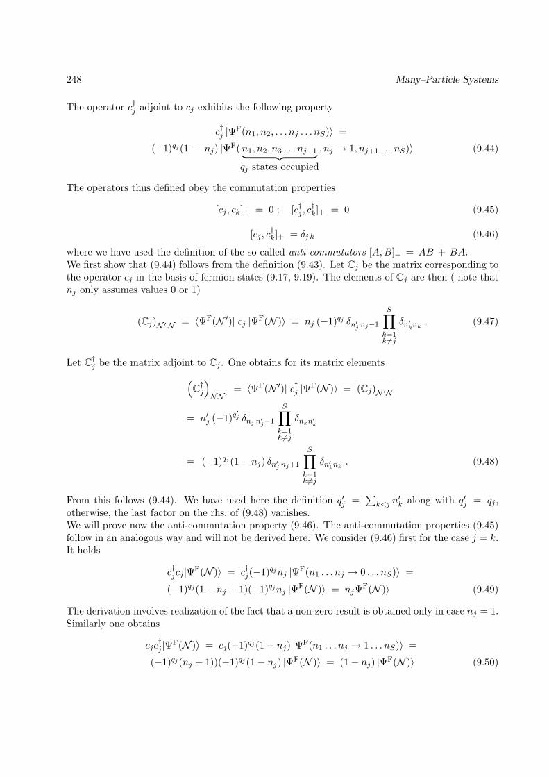
248 Many–Particle Systems
The operator c†j adjoint to cj exhibits the following property
c†j |ΨF(n1, n2, . . . nj . . . nS)〉 =
(−1)qj (1 − nj) |ΨF(n1, n2, n3 . . . nj−1︸ ︷︷ ︸qj states occupied
, nj → 1, nj+1 . . . nS)〉 (9.44)
The operators thus defined obey the commutation properties
[cj , ck]+ = 0 ; [c†j , c†k]+ = 0 (9.45)
[cj , c†k]+ = δj k (9.46)
where we have used the definition of the so-called anti-commutators [A,B]+ = AB + BA.We first show that (9.44) follows from the definition (9.43). Let Cj be the matrix corresponding tothe operator cj in the basis of fermion states (9.17, 9.19). The elements of Cj are then ( note thatnj only assumes values 0 or 1)
(Cj)N ′N = 〈ΨF(N ′)| cj |ΨF(N )〉 = nj (−1)qj δn′j nj−1
S∏k=1k 6=j
δn′knk . (9.47)
Let C†j be the matrix adjoint to Cj . One obtains for its matrix elements(C†j
)NN ′
= 〈ΨF(N ′)| c†j |ΨF(N )〉 = (Cj)N ′N
= n′j (−1)q′j δnj n′j−1
S∏k=1k 6=j
δnkn′k
= (−1)qj (1− nj) δn′j nj+1
S∏k=1k 6=j
δn′knk . (9.48)
From this follows (9.44). We have used here the definition q′j =∑
k<j n′k along with q′j = qj ,
otherwise, the last factor on the rhs. of (9.48) vanishes.We will prove now the anti-commutation property (9.46). The anti-commutation properties (9.45)follow in an analogous way and will not be derived here. We consider (9.46) first for the case j = k.It holds
c†jcj |ΨF(N )〉 = c†j(−1)qjnj |ΨF(n1 . . . nj → 0 . . . nS)〉 =
(−1)qj (1− nj + 1)(−1)qjnj |ΨF(N )〉 = njΨF(N )〉 (9.49)
The derivation involves realization of the fact that a non-zero result is obtained only in case nj = 1.Similarly one obtains
cjc†j |ΨF(N )〉 = cj(−1)qj (1− nj) |ΨF(n1 . . . nj → 1 . . . nS)〉 =
(−1)qj (nj + 1))(−1)qj (1− nj) |ΨF(N )〉 = (1− nj) |ΨF(N )〉 (9.50)

9.2: Operators of 2nd Quantization 249
(9.49) and (9.50) yield( cjc
†j + c†jcj ) |ΨF(N )〉 = |ΨF(N )〉 . (9.51)
For j < k one obtains
cjc†k|Ψ
F(N )〉 = (−1)qj+qknj(1− nk)|ΨF(n1 . . . nj = 0 . . . nk = 1 . . . nS)〉c†kcj |Ψ
F(N )〉 = (−1)qj+qk−1nj(1− nk)|ΨF(n1 . . . nj = 0 . . . nk = 1 . . . nS)〉
and, hence,( cjc
†k + c†kcj ) |ΨF(N )〉 = 0 . (9.52)
One can obtain similarly the same relationship in the case j > k. Since (9.51, 9.52) hold for any|ΨF(N )〉 one can conclude (9.46).Equation (9.49) shows that the operator
Nj = c†jcj (9.53)
is diagonal in the occupation number representation, i.e., in the basis |ΨF(N )〉, with eigenvaluesequal to the occupation numbers nj
Nj |ΨF(N )〉 = nj |ΨF(N )〉 (9.54)
Nj , hence, is referred to as the occupation number operator. Correspondingly,
N =S∑j=1
Nj (9.55)
is called the particle number operator.It is an interesting exercise to demonstrate that Nj only has eigenvalues 0 or 1, for which purposeone needs to envoke only the algebraic (anti-commutation) properties (9.46). The stated propertyfollows from the idempotence of Nj which can be derived as follows
N2j = c†jcjc
†jcj = c†j (1− c†jcj)cj = c†jcj − c†jc
†jcjcj = c
†jcj = Nj . (9.56)
Here we have made use of cjcj = 0 and c†jc†j = 0 which follows from nj ∈ 0, 1.
We finally note that the creation operators c†j allow one to construct any fermion state |ΨF(N )〉from the vacuum state |0〉 defined as above (see (9.29))
|ΨF(. . . nλ1 . . . nλ2 . . . nλN . . .)〉 = c†λ1c†λ2· · · c†λN |0〉 . (9.57)
On the l.h.s. of this equation we meant to indicate only those N occupation numbers nλj whichare non-vanishing. On the r.h.s. the creation operators must operate in the proper order, i.e., anoperator cj must be on the left of an operator ck for j < k.In the following we will apply fermion operators c†j and cj only to electrons which carry spin 1
2 . Wewill often separate the states |j〉, coordinates ~x and index j into a space part and a spin part, i.e.,
j → j, σ (σ = ± 12) ; 〈~x|j〉 → φj(~r) | 12σ〉 . (9.58)
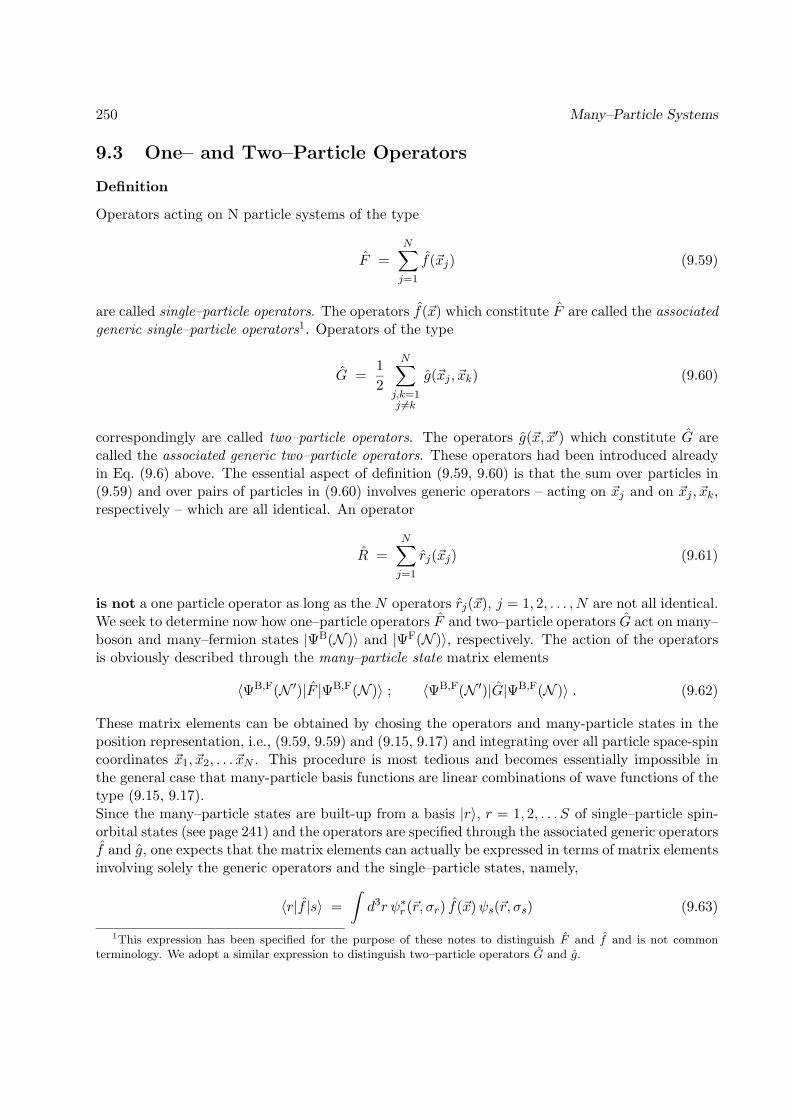
250 Many–Particle Systems
9.3 One– and Two–Particle Operators
Definition
Operators acting on N particle systems of the type
F =N∑j=1
f(~xj) (9.59)
are called single–particle operators. The operators f(~x) which constitute F are called the associatedgeneric single–particle operators1. Operators of the type
G =12
N∑j,k=1j 6=k
g(~xj , ~xk) (9.60)
correspondingly are called two–particle operators. The operators g(~x, ~x′) which constitute G arecalled the associated generic two–particle operators. These operators had been introduced alreadyin Eq. (9.6) above. The essential aspect of definition (9.59, 9.60) is that the sum over particles in(9.59) and over pairs of particles in (9.60) involves generic operators – acting on ~xj and on ~xj , ~xk,respectively – which are all identical. An operator
R =N∑j=1
rj(~xj) (9.61)
is not a one particle operator as long as the N operators rj(~x), j = 1, 2, . . . , N are not all identical.We seek to determine now how one–particle operators F and two–particle operators G act on many–boson and many–fermion states |ΨB(N )〉 and |ΨF(N )〉, respectively. The action of the operatorsis obviously described through the many–particle state matrix elements
〈ΨB,F(N ′)|F |ΨB,F(N )〉 ; 〈ΨB,F(N ′)|G|ΨB,F(N )〉 . (9.62)
These matrix elements can be obtained by chosing the operators and many-particle states in theposition representation, i.e., (9.59, 9.59) and (9.15, 9.17) and integrating over all particle space-spincoordinates ~x1, ~x2, . . . ~xN . This procedure is most tedious and becomes essentially impossible inthe general case that many-particle basis functions are linear combinations of wave functions of thetype (9.15, 9.17).Since the many–particle states are built-up from a basis |r〉, r = 1, 2, . . . S of single–particle spin-orbital states (see page 241) and the operators are specified through the associated generic operatorsf and g, one expects that the matrix elements can actually be expressed in terms of matrix elementsinvolving solely the generic operators and the single–particle states, namely,
〈r|f |s〉 =∫d3r ψ∗r (~r, σr) f(~x)ψs(~r, σs) (9.63)
1This expression has been specified for the purpose of these notes to distinguish F and f and is not commonterminology. We adopt a similar expression to distinguish two–particle operators G and g.

9.3: One– and Two–Particle Operators 251
〈r, s|g|t, u〉 =∫d3r
∫d3r′ ψ∗r (~r, σr)ψ
∗s(~r′, σs) g(~x, ~x ′)ψt(~r, σt)ψu(~r ′, σu) . (9.64)
We like to note an important symmetry of the matrix element 〈r, s|g|t, u〉 which follows directlyfrom the definition (9.64)
〈r, s|g|t, u〉 = 〈s, r|g|u, t〉 . (9.65)
This symmetry will be exploited repeatedly below. Notice, that the symmetry implies that one canswitch simultaneously the pairs of indices r, s and t, u, one cannot switch the indices of one pairindividually.The aim of the present section is to express the matrix elements of single– and two–particle operatorsin a basis of many–particle states (9.62) in terms of the matrix elements of single–particle states(9.63, 9.64). We will show that the boson and fermion creation and annihilation operators servethis purpose.
Examples of One– and Two–Particle Operators
An example for a single–particle operator is the kinetic energy operator
T =N∑j=1
(− ~
2
2m
)∂2
∂~r 2j
. (9.66)
Here we adopt the notation for the Laplacian
∂2
∂~r 2=
∂2
∂x21
+∂2
∂x22
+∂2
∂x23
. (9.67)
In this case the generic single–particle operator, according to (9.59), is t(~x) = (−~2/2m)(∂2/∂~r 2).The matrix elements of this operator in a single–particle basis are
〈rσ|t|sσ′〉 = δσσ′
∫d3r φ∗r(~r)
(− ~
2
2m
)∂2
∂~r 2φs(~r) . (9.68)
Another single–particle operator is the one–particle density operator
ρ(~r′) =
N∑j=1
δ(~r − ~rj) . (9.69)
In this case the generic operator is f(~x) = δ(~r − ~r). The matrix elements of the generic operatorin the one–particle basis are
〈rσ|f |sσ′〉 = δσσ′
∫d3r φ∗r(~r) δ(~r − ~r)φs(~r) = δσσ′ φ
∗r(~r)φs(~r) δσσ′ (9.70)
Both operators, i.e., (9.66) and (9.69), are spin-independent as is evident from the factor δσσ′ .An example for a two–particle operator is the Coulomb repulsion operator
V =12
N∑j,k=1j 6=k
q2
|~rj − ~rk|(9.71)

252 Many–Particle Systems
which is also spin-independent. In this case the generic operator is v(~x, ~x′) = q2/|~r1 − ~r2|. Thematrix elements of the generic operator in terms of single–particle states are
〈r, σ; s, σ′| t |t, σ′′; u, σ′′′〉 =∫d3r1
∫d3r2 φ
∗r(~r1)φ∗s(~r2) q2
|~r1 − ~r2|φt(~r1)φu(~r2) δσσ′′δσ′σ′′′ (9.72)
As a final example of one– and two–particle operators we consider operators of total spin. Theoperator
~S =N∑j=1
~Sj (9.73)
is a one-particle operator. Here, ~Sj is the spin operator for particle j with components (in thespherical representation) Sj,+, Sj,−, Sj,3. The generic operator is given through the Pauli matrices,i.e., ~s = 1
2~σ. The non-vanishing matrix elements of the spherical components of ~s are (α = +12 , β =
−12)
〈r, α|s+|s, β〉 = δrs
〈r, β|s−|s, α〉 = δrs
〈r, α|s3|s, α〉 = + 12δrs
〈r, β|s3|s, β〉 = − 12δrs (9.74)
The operator
S2 =
N∑j=1
~Sj
2
=N∑
j,k=1
~Sj · ~Sk (9.75)
is a two–particle operator, however, not in the strict sense of our definition above since the restrictionj 6= k does not apply in the summation. However, one can obviously extract the term
∑j S
2j to be
left with a two–particle operator in the strict sense of our definition. The generic operator is
s12 = ~S1 · ~S2 =12S1,+S2,− +
12S1,−S2,+ + S1,3S2,3 (9.76)
the single–particle state matrix elements of which are
〈r, σ; s, σ′| s12 |t, σ′′; u, σ′′′〉 = δrt δsu
(12δ 1
2σδ− 1
2σ′′δ− 1
2σ′δ 1
2σ′′′ +
+ 12δ− 1
2σδ 1
2σ′′δ 1
2σ′δ− 1
2σ′′′ + 1
4 δσσ′′δσ′σ′′′ ( δσσ′ − δ−σσ′ )). (9.77)
The operators (9.74) and (9.77) are orbital-independent as evidenced by the factors δrs and δrtδsuin the respective formulas.
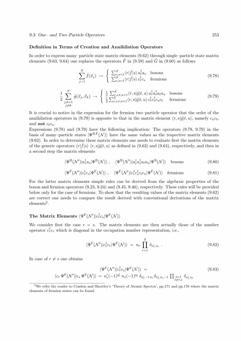
9.3: One– and Two–Particle Operators 253
Definition in Terms of Creation and Annihilation Operators
In order to express many–particle state matrix elements (9.62) through single–particle state matrixelements (9.63, 9.64) one replaces the operators F in (9.59) and G in (9.60) as follows
N∑j=1
f(~xj) →
∑Sr,s=1〈r|f |s〉 a
†ras bosons∑S
r,s=1〈r|f |s〉 c†rcs fermions
(9.78)
12
N∑j,k=1j 6=k
g(~xj , ~xk) →
12
∑Sr,s,t,u=1〈r, s|g|t, u〉 a
†ra†satau bosons
12
∑Sr,s,t,u=1〈r, s|g|t, u〉 c
†rc†scuct fermions
(9.79)
It is crucial to notice in the expression for the fermion two–particle operator that the order of theannihilation operators in (9.79) is opposite to that in the matrix element 〈r, s|g|t, u〉, namely cuct,and not ctcu.Expressions (9.78) and (9.79) have the following implication: The operators (9.78, 9.79) in thebasis of many–particle states |ΨB,F(N )〉 have the same values as the respective matrix elements(9.62). In order to determine these matrix elements one needs to evaluate first the matrix elementsof the generic operators 〈r|f |s〉 〈r, s|g|t, u〉 as defined in (9.63) and (9.64), respectively, and then ina second step the matrix elements
〈ΨB(N ′)|a†ras|ΨB(N )〉 , 〈ΨB(N ′)|a†ra†satau|ΨB(N )〉 bosons (9.80)
〈ΨF(N ′)|c†rcs|ΨF(N )〉 , 〈ΨF(N ′)|c†rc†sctcu|ΨF(N )〉 fermions (9.81)
For the latter matrix elements simple rules can be derived from the algebraic properties of theboson and fermion operators (9.23, 9.24) and (9.45, 9.46), respectively. These rules will be providedbelow only for the case of fermions. To show that the resulting values of the matrix elements (9.62)are correct one needs to compare the result derived with conventional derivations of the matrixelements2.
The Matrix Elements 〈ΨF(N ′)|c†rcs|ΨF(N )〉
We consider first the case r = s. The matrix elements are then actually those of the numberoperator c†rcr which is diagonal in the occupation number representation, i.e.,
〈ΨF(N ′)|c†rcr|ΨF(N )〉 = nr
S∏r=1
δn′r nr . (9.82)
In case of r 6= s one obtains
〈ΨF(N ′)|c†rcs|ΨF(N )〉 = (9.83)〈cr ΨF(N ′)|cs ΨF(N )〉 = n′r(−1)q
′r ns(−1)qs δn′r−1nrδn′s ns−1
∏t=1t6=r,s
δn′t nt
2We refer the reader to Condon and Shortley’s ‘Theory of Atomic Spectra’, pp.171 and pp.176 where the matrixelements of fermion states can be found.
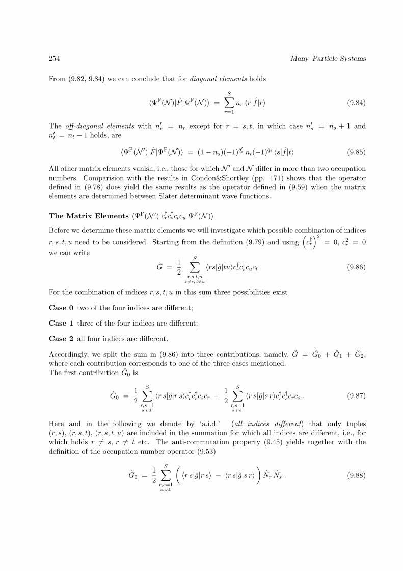
254 Many–Particle Systems
From (9.82, 9.84) we can conclude that for diagonal elements holds
〈ΨF(N )|F |ΨF(N )〉 =S∑r=1
nr 〈r|f |r〉 (9.84)
The off-diagonal elements with n′r = nr except for r = s, t, in which case n′s = ns + 1 andn′t = nt − 1 holds, are
〈ΨF(N ′)|F |ΨF(N )〉 = (1− ns)(−1)q′s nt(−1)qt 〈s|f |t〉 (9.85)
All other matrix elements vanish, i.e., those for which N ′ and N differ in more than two occupationnumbers. Comparision with the results in Condon&Shortley (pp. 171) shows that the operatordefined in (9.78) does yield the same results as the operator defined in (9.59) when the matrixelements are determined between Slater determinant wave functions.
The Matrix Elements 〈ΨF(N ′)|c†rc†sctcu|ΨF(N )〉
Before we determine these matrix elements we will investigate which possible combination of indices
r, s, t, u need to be considered. Starting from the definition (9.79) and using(c†r)2
= 0, c2r = 0
we can write
G =12
S∑r,s,t,ur 6=s, t6=u
〈rs|g|tu〉c†rc†scuct (9.86)
For the combination of indices r, s, t, u in this sum three possibilities exist
Case 0 two of the four indices are different;
Case 1 three of the four indices are different;
Case 2 all four indices are different.
Accordingly, we split the sum in (9.86) into three contributions, namely, G = G0 + G1 + G2,where each contribution corresponds to one of the three cases mentioned.The first contribution G0 is
G0 =12
S∑r,s=1a.i.d.
〈r s|g|r s〉c†rc†scscr +12
S∑r,s=1a.i.d.
〈r s|g|s r〉c†rc†scrcs . (9.87)
Here and in the following we denote by ‘a.i.d.’ (all indices different) that only tuples(r, s), (r, s, t), (r, s, t, u) are included in the summation for which all indices are different, i.e., forwhich holds r 6= s, r 6= t etc. The anti-commutation property (9.45) yields together with thedefinition of the occupation number operator (9.53)
G0 =12
S∑r,s=1a.i.d.
(〈r s|g|r s〉 − 〈r s|g|s r〉
)Nr Ns . (9.88)
9.3: One– and Two–Particle Operators 255
Obviously, this contribution to the two–particle operator is diagonal in the occupation numberrepresentation. As we will find, this part accounts for all diagonal contributions to G.The second contribution G1 is
G1 = 12
∑Sr,s,t=1
a.i.d.
〈r s|g|r t〉c†rc†sctcr
+ 12
∑Sr,s,t=1
a.i.d.
〈r s|g|t s〉c†rc†scsct
+ 12
∑Sr,s,t=1
a.i.d.
〈r s|g|s t〉c†rc†sctcs
+ 12
∑Sr,s,t=1
a.i.d.
〈r s|g|t r〉c†rc†scrct . (9.89)
Commutation of ctcu according to (9.45), employing the symmetry property (9.65), relabellingsummation indices and using c†rc
†sctcr = c†sc
†rcrct = c†sctNr yields
G1 =S∑
r,s,t=1a.i.d.
(〈r s|g|r t〉 − 〈r s|g|t r〉
)c†sctNr . (9.90)
Since Nr is diagonal, this contribution obviously behaves similarly to the off-diagonal part (9.84)of the one–particle operator F .A similar series of transformations allows one to express G2 which can be written
G2 = 12
∑Sr,s,t,ur>s,t>u
〈r s|g|t u〉c†rc†scuct
+ 12
∑Sr,s,t,ur>s,t<u
〈r s|g|t u〉c†rc†scuct
+ 12
∑Sr,s,t,ur<s,t>u
〈r s|g|t u〉c†rc†scuct
+ 12
∑Sr,s,t,ur<s,t<u
〈r s|g|t u〉c†rc†scuct (9.91)
as follows
G2 =S∑
r,s,t,ur>s,t>u
(〈r s|g|t u〉 − 〈r s|g|u t〉
)c†rc†scuct . (9.92)
This contribution to G has non-vanishing matrix elements only when N ′ differs from N in fouroccupation numbers nr, ns, nt, nu. A similar contribution does not arise for F .We can state now the matrix elements 〈ΨF(N ′)|G|ΨF(N )〉. For this purpose we consider threecases which actually correspond to the three cases considered below Eq. (9.86).
Case 0 This case covers diagonal matrix elements, i.e., N ′ = N or n′r = nr for all r. Only G0,given in (9.88), contributes in this case. One obtains
〈ΨF(N )|G|ΨF(N )〉 =12
S∑r,s
nrns
(〈r, s|g|r, s〉 − 〈r, s|g|s, r〉
). (9.93)
256 Many–Particle Systems
Case 1 This case covers off-diagonal elements with n′r = nr except for r = s, t for which holdsn′s = ns + 1 and n′t = nt− 1. Only G1, given in (9.90), contributes in this case. One obtains
〈ΨF(N ′)|G|ΨF(N )〉 =
(−1)q′s+qt(1− ns)nt
∑r
r 6=s,tnr
(〈r, s|g|r, t〉 − 〈r, s|g|t, r〉
)(9.94)
Case 2 This case covers off-diagonal elements with n′r = nr except for r = s, t, u, v for which holdsn′s = ns + 1, n′t = nt + 1, n′u = nu − 1, n′v = nv − 1. Only G2, given in (9.92), contributesin this case. One obtains
〈ΨF(N ′)|G|ΨF(N )〉 = (9.95)
± (−1)q′s+q
′r+qu+qv(1− ns)(1− nr)nunv
(〈r, s|g|u, v〉 − 〈r, s|g|v, u〉
)In the latter formula the ‘+’-sign applies for s < r, u < v or s > r, u > v, the ‘−’-sign appliesfor s < r, u > v or s > r, u < v.
All matrix elements which are not covered by the three cases above vanish. In particular, fornon-vanishing matrix elements 〈ΨF(N ′)|G|ΨF(N )〉 at most four occupation numbers n′r and nr candiffer. Furthermore, particle number is conserved, i.e., it holds
∑Sr=1 n
′r =
∑Sr=1 nr.
Exercise 9.3.1: Derive (9.90) from (9.89).Exercise 9.3.2: Derive (9.92) from (9.91).Exercise 9.3.3: Derive (9.95) from (9.92).Exercise 9.3.4: Show that the matrix elements of F and of G conserve particle number.Exercise 9.3.5: Derive the non-vanishing matrix elements (9.62) for bosons.
Spin Operators
In this section we will briefly consider the spin operators ~S given in (9.73) and S2 given in (9.75)which are, respectively, one–particle and two–particle operators. The matrix elements of the cor-responding generic operators are (9.74) and (9.76). We like to express these operators through
fermion creation and annihilation operators. One obtains for the three components of ~S
S3 =12
S∑r=1
(Nrα − Nrβ
)S+ =
S∑r=1
c†rαcrβ
S− =S∑r=1
c†rβcrα (9.96)

9.4: Independent-Particle Models 257
For S2 one obtains
S2 =12N +
14
S∑r,s=1
(Nrα − Nrβ)(Nsα − Nsβ) −S∑
r,s=1
c†rαc†sβcrβcsα . (9.97)
The summation in (9.96, 9.97) is over the orbital states, the spin part of the single–particle statesis represented by α = 1
2 and β = −12 .
Exercise 9.3.6: Derive (9.96) and (9.97).
9.4 Independent-Particle Models
In the remaining part of this chapter we will apply the technique of operators of 2nd quantizationto the description of many–fermion systems as they arise, e.g., in crystals, molecules, atoms andnuclei. In all these systems the Hamiltonian is a sum of one– and two–particle operators
H =S∑r=1
〈r|t|s〉c†rcs +12
S∑r,s,t,u
〈r, s|v|u, v〉c†rc†scuct . (9.98)
In many cases the Hamiltonian is spin-independent and the equivalent notation
H =S∑
r,s=1σ
〈r|t|s〉c†rσcsσ +12
S∑r,s,t,u=1σ,σ′
〈r, s|v|t, u〉c†rσc†sσ′cuσ′ctσ (9.99)
will be used. In the latter case the indices r, s, t, u refer only to the orbital part of the single–particlebasis.If it were not for the two–particle contribution to the Hamiltonian, which represents the interactionsbetween particles, the description of many–particle systems, e.g., evaluation of their stationarystates and excitation energies, would be a simple exercise in linear algebra. Unfortunately, thetwo–particle operator makes the description of many–particle systems a very hard problem. Thefortunate side of this is, however, that the two–particle operator representing interactions betweenparticles induces a variety of interesting phenomena.Actually, the study of problems governed by Hamiltonians of the type (9.98, 9.99) has preoccupiedan important part of all intellectual efforts in Theoretical Physics during the past fifty years. Infact, it is one of the main intellectual achievements of Physics among the Sciences to have addressedsystematically the study of systems composed of many strongly interacting components. The out-come of these studies is that even when interactions between components (particles) are simple,the concerted behaviour of interacting systems can deviate qualitatively from that of systems madeup of independent components. Examples is the laser action, superconductivity, but also ordinaryphenomena like freezing and evaporation. Often, the systems investigated involve a macroscopicnumber of components such that statistical mechanical approaches are envoked. The great general-ity of the concepts developed in the context of many–particle systems can be judged from the fact

258 Many–Particle Systems
that today these concepts are providing insight into the functioning of biological brains, anotherprototypical systems of many strongly interacting components, namely of neurons3.Before continuing one may finally point out that the material world as we know it and as itestablishes the varieties of natural substances, ranging from nuclei to the molecules of living systems, ultimately depend in a crucial way on the fermion character of its constituent building blocks,electrons and nucleons. If it were’nt for the fermion nature, all material systems would condensateinto states which would depend little on particle number. The Aufbau principle, according to whichnuclei and atoms change their qualitative properties when they grow larger, would not exist. Theelectronic properties of atoms with different numbers of electrons would differ little, Chemistryessentially would know only one element and Life would not exist.
Exercise 9.4.1: Imagine that in a closed, water-filled jar all electrons of water turn their fermionnature into a boson nature. What might happen?
Independent-Particle Hamiltonian
A many–fermion system governed by an independent-particle Hamiltonian, i.e., a Hamiltonianwithout a two–particle operator contribution accounting for interactions among the particles, canbe described in a rather straightforward way. We will restrict our description in the following tosystems composed of an even number (2N) of particles and to spin-independent interactions. TheHamiltonian of such system is
Ho =S∑
r,s=1σ
〈r|t|s〉c†rσcsσ (9.100)
We will denote the matrix elements of t as 〈r|t|s〉 = trs.
Transformation to a New Set of Creation and Annihilation Operators
Our aim is to represent the Hamiltonian (9.100) in a form in which the factors c†rσcsσ becomeoccupation number operators. In such a representation Ho is diagonal and the stationary statescan be stated readily. To alter the representation of Ho we apply a unitary transformation U tothe single–particle states |r〉 to obtain a new basis of states |m), i.e., |m),m = 1, 2, . . . S, where
|m) =S∑r=1
Urm|r〉 . (9.101)
The unitary property of UrnU†U = U U† = 11 (9.102)
orS∑r=1
U ∗rm Urn = δmn ,
S∑m=1
UrmU∗sm = δrs (9.103)
3An account of some of these efforts can be found in Modelling Brain Function – The World of Attractor NeuralNetworks by D.J. Amit (Cambridge University Press, New York, 1989)
9.4: Independent-Particle Models 259
allows one to express conversely |r〉 in terms of |m)
|r〉 =S∑
m=1
U∗rm|m) . (9.104)
One can, hence, expand
trs =S∑mn
tmnUrmU∗sn (9.105)
where
tmn = (m|t|n) =S∑
r,s=1
trsU∗rmUsn =
(U †tU
)mn
(9.106)
which together with (9.100) yieldsHo = tmnd
†mσdnσ (9.107)
where
d†nσ =S∑r=1
Urnc†rσ , dnσ =
S∑r=1
U∗rncrσ (9.108)
These operators describe the creation and annihilation operators of fermions in states |n) whichare linear combinations (9.101) of states |r〉. The unitary property (9.103) allows one to express[c.f. (9.104)]
c†rσ =S∑
m=1
U∗rmd†mσ , csσ =
S∑n=1
Usndnσ . (9.109)
The operators (9.108) obey the same anti-commutation properties (9.45, 9.46) as c†rσ and crσ,namely,
[dmσ, dnσ′ ]+ = 0 ; [d†mσ, d†nσ′ ]+ = 0 (9.110)
[dmσ, d†nσ′ ]+ = δmn δσσ′ (9.111)
and, accordingly, they are Fermion creation and annihilation operators. In a basis of states
N∏j=1
d†njσj |0〉 (9.112)
, i.e., of N -Fermion states in which single particle states |nj) as defined in (9.101) are occupied, theoperators d†nσ and dnσ, behave exactly like the operators c†rσ and crσ behave for states |ΨF (N )〉; forexample, the expressions drived above for the matrix elements of one- and two-particle operatorshold in an analogous way for d†nσ and dnσ.We demonstrate here the anti-commutation property (9.111), the anti-commutation properties(9.110) can be demonstrated similarly. The l.h.s. of (9.111) can be written, using (9.108) and(9.46),
[dmσ, d†nσ′ ]+ =
∑r,s
U∗rmUsn [crσ, c†sσ′ ]+ = δσσ′
∑r
U∗rmUrn . (9.113)
The unitarity property∑
r U∗rmUrn = δmn yields immediately identity (??).

260 Many–Particle Systems
Diagonal Representation
The transformation (9.101) gives us the freedom to choose the matrix (9.106) diagonal, i.e.,
tmn = εn δmn . (9.114)
In this case Ho has the desired form
Ho =S∑n=1
εnd†nσdnσ (9.115)
and involves solely occupation number operators Nnσ = d†nσdnσ. It is, hence, a simple matter tostate many–particle states in the new representation.Before proceeding we like to address the issue how the new representation, i.e., transformationmatrices Urn and energy values εn, is obtained. The condition (9.114) together with (9.106) isequivalent to
S∑s=1
trsUsn = εnUrn ∀r, r = 1, 2, . . . S (9.116)
which follows from (9.106) and the unitary property of Urn. This equation poses the eigenvalueproblem for the hermitian matrix (trs). The corresponding eigenvalues εn, n = 1, 2, . . . S arereal, the associated ( properly normalized) eigenvectors Vn are the columns of (Urn), i.e., V T
n =(U1n, U2n, . . . USn).Eigenstates of (9.115) can be stated immediately since any many–particle wave function in theoccupation number representation is suitable. We apply for this purpose (9.57) to the case of 2Nparticles. The 2N fermion state
2N∏j=1
d†nj σj |0〉 where (nj , σj) 6= (nk, σk) for j 6= k (9.117)
are eigenstates of (9.115) with eigenvalues
E(n1, σ1; n2, σ2; . . . n2N , σ2N ; ) =2N∑j=1
εnj . (9.118)
Ground State
In case of an ordering εm < εn for m < n the state of lowest energy, the so-called ground state, is
|Φo〉 =N∏j=1
d†j αd†j β |0〉 . (9.119)
In this state the N lowest orbital eigenstates of trs are occupied each by an electron with spin|α〉 = |12 ,
12〉 and |β〉 = |12 ,−
12〉. A non-degenerate orbital state which is occupied by two fermions,
i.e., a fermion in a spin state |12 ,12〉 as well as a fermion in a spin state |12 , −
12〉 is called a closed
9.4: Independent-Particle Models 261
shell. The ground state has only closed shells. We will demonstrate now that this property endowsthe ground state with total spin zero.In order to investigate the total spin of |Φo〉 we apply to this state the total spin operator S2 asgiven by (9.97). The spin operator in the present representation of single-particle states is
S2 =12N +
14
S∑m,n=1
( Nmα − Nmβ)( Nnα − Nnβ) −S∑
m,n=1
d†mαd†nβdmβdnα (9.120)
where the occupation number operators refer to the single-particle states |m). The action of theoperator (9.120) is particularly simple for closed shells. One can conclude immediately that the
second term in (9.97), namely, 14
∑Sm,n=1( Nmα − Nmβ)( Nnα − Nnβ) does not give any contribution
if either |m) or |n) are closed shells. Similarly, the third term −∑S
m,n=1 c†mαc
†nβcmβcnα does not
give a contribution if m 6= n and either |m) or |n) are closed shells. In case of m = n it gives acontribution ‘1’ for each closed shell which cancels the contribution of the first term. Alltogether,one can conclude that |Φo〉 is an eigenstate of S2 with eigenvalue zero, i.e., is a singlet state.
Excited States
We want to construct now excited states for the system governed by the independent-particleHamiltonian (9.100). Obviously, the states with energy closest to the ground state are those inwhich a particle is promoted from the highest occupied state |N) to the lowest unoccupied state|N + 1). There are four such states, namely,
|α, α〉〉 = d†N+1αdNα|Φo〉
|α, β〉〉 = d†N+1αdNβ|Φo〉
|β, α〉〉 = d†N+1βdNα|Φo〉
|β, β〉〉 = d†N+1βdNβ|Φo〉 (9.121)
All four states have the same excitation energy, i.e., energy above the ground state, of ∆E =εN+1 − εN . However, the states differ in their spin character. The two states |α, β〉〉 and |β, α〉〉are eigenstates of S2 given in (9.120), both with eigenvalues 2
S2|α, β〉〉 = 2 |α, β〉〉 ; S2||β, α〉〉 = 2 |β, α〉〉 . (9.122)
This property can be derived as follows: The two states are obviously diagonal with respect to thefollowing contribution to S2
Σ1 =12N +
14
N−1∑m,n=1
(Nmα − Nmβ)(Nnα − Nnβ) −N−1∑m,n=1
d†mαd†nβdmβdnα (9.123)
which acts only on the N − 1 closed shells (except for N) of the two states and has an eigenvalueN + 0 − (N − 1) = 1 in both cases. The remaining contributions to S2 which act on partiallyoccupied orbitals |N〉 and |N + 1〉 are
Σ2 =14
N+1∑m,n=N
(Nmα − Nmβ)(Nnα − Nnβ) (9.124)
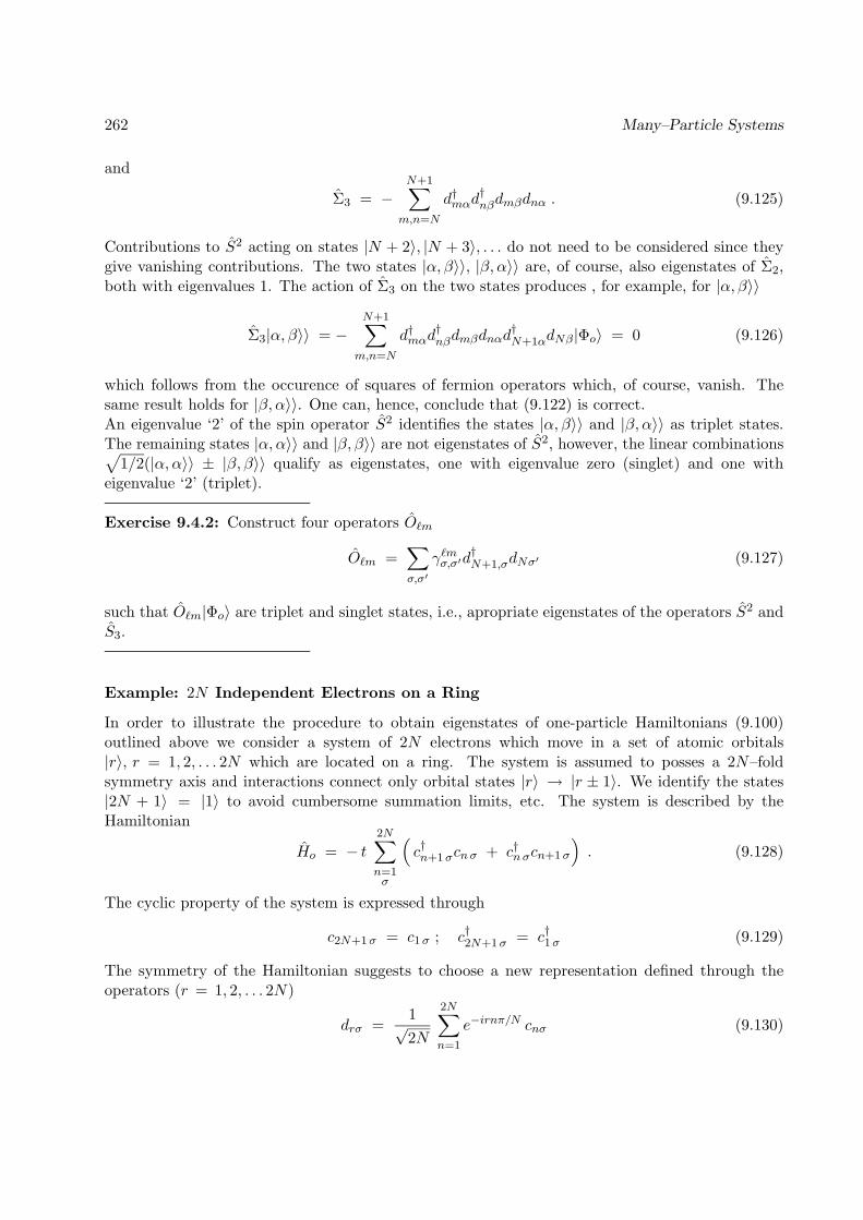
262 Many–Particle Systems
and
Σ3 = −N+1∑m,n=N
d†mαd†nβdmβdnα . (9.125)
Contributions to S2 acting on states |N + 2〉, |N + 3〉, . . . do not need to be considered since theygive vanishing contributions. The two states |α, β〉〉, |β, α〉〉 are, of course, also eigenstates of Σ2,both with eigenvalues 1. The action of Σ3 on the two states produces , for example, for |α, β〉〉
Σ3|α, β〉〉 = −N+1∑m,n=N
d†mαd†nβdmβdnαd
†N+1αdNβ|Φo〉 = 0 (9.126)
which follows from the occurence of squares of fermion operators which, of course, vanish. Thesame result holds for |β, α〉〉. One can, hence, conclude that (9.122) is correct.An eigenvalue ‘2’ of the spin operator S2 identifies the states |α, β〉〉 and |β, α〉〉 as triplet states.The remaining states |α, α〉〉 and |β, β〉〉 are not eigenstates of S2, however, the linear combinations√
1/2(|α, α〉〉 ± |β, β〉〉 qualify as eigenstates, one with eigenvalue zero (singlet) and one witheigenvalue ‘2’ (triplet).
Exercise 9.4.2: Construct four operators O`m
O`m =∑σ,σ′
γ`mσ,σ′d†N+1,σdNσ′ (9.127)
such that O`m|Φo〉 are triplet and singlet states, i.e., apropriate eigenstates of the operators S2 andS3.
Example: 2N Independent Electrons on a Ring
In order to illustrate the procedure to obtain eigenstates of one-particle Hamiltonians (9.100)outlined above we consider a system of 2N electrons which move in a set of atomic orbitals|r〉, r = 1, 2, . . . 2N which are located on a ring. The system is assumed to posses a 2N–foldsymmetry axis and interactions connect only orbital states |r〉 → |r ± 1〉. We identify the states|2N + 1〉 = |1〉 to avoid cumbersome summation limits, etc. The system is described by theHamiltonian
Ho = − t2N∑n=1σ
(c†n+1σcnσ + c†nσcn+1σ
). (9.128)
The cyclic property of the system is expressed through
c2N+1σ = c1σ ; c†2N+1σ = c†1σ (9.129)
The symmetry of the Hamiltonian suggests to choose a new representation defined through theoperators (r = 1, 2, . . . 2N)
drσ =1√2N
2N∑n=1
e−irnπ/N cnσ (9.130)

9.4: Independent-Particle Models 263
d†rσ =1√2N
2N∑n=1
eirnπ/N c†nσ (9.131)
(9.130, 9.131) constitute a unitary transformation U defined through Urn = 1√2Neirnπ/N . The
unitarity property follows from
2N∑r=1
eirsπ/N = 0 for 0 < s < 2N . , (9.132)
an identity which can be derived employing the well-known expression for a finite geometric series
m∑s=1
as = a1− am
1− a. (9.133)
Application to the l.h.s. of (9.132) gives for r 6= 0, 2N, 4N, . . .
eisπ/N1 − e2N isπ/N
1 − eisπ/N(9.134)
which, indeed, vanishes for integer s. One can then express[.f. (9.109)]
cnσ =1√2N
2N∑r=1
eirnπ/N drσ (9.135)
c†nσ =1√2N
2N∑r=1
e−irnπ/N d†rσ (9.136)
and, thereby, one obtains the new representation of Ho
Ho = −t2N∑r,s=1σ
trs d†rσdsσ (9.137)
where
trs = e−irπ/N1
2N
2N∑n=1
ei(s−r)nπ/N + eisπ/N1
2N
2N∑n=1
ei(r−s)nπ/N . (9.138)
Using (9.132) one can conclude
trs =(eirπ/N + e−irπ/N
)δrs (9.139)
from which follows
Ho =2N∑r=1σ
(−2t cos
rπ
N
)d†rσdrσ . (9.140)
The Hamiltonian is now diagonal and the construction outlined above can be applied.

264 Many–Particle Systems
Exercise 9.4.3: Construct the ground state and the lowest energy excited state(s) for a sys-tem of 2N electrons moving in a linear chain of single-electron orbitals |n〉, n = 1, 2, . . . 2N withinteractions between neighbouring (n, n± 1) orbitals and Hamiltonian
Ho = − t2N−1∑n=1σ
(c†n+1σcnσ + c†nσcn+1σ
). (9.141)
State the excitation energy ∆E.
9.5 Self-Consistent Field Theory
Observations of many-fermion systems show that properties of such systems often can be explainedto a surprisingly good degree on the basis of the assumption that the fermions move like independentparticles. The most famous example is the periodic table of the elements. The regularities of theelements can be rationalized in terms of electrons moving in hydrogen atom-type orbitals, i.e.,in states which are constructed according to the ‘Aufbauprinzip’ in a manner which neglects themutual repulsion between electrons. A similar principle accounts approximately for properties ofnuclei as described by the nuclear shell model. The properties of molecules can be understoodlargely in terms of models which place electrons into so-called molecular orbitals in which theelectrons move as if they were not interacting with other electrons. Many electronic propertiesof solids can be understood in a similar way, i.e., assuming that electrons move independentlyfrom each other in so-called bands, e.g., valence bands or conduction bands. Of course, propertiesof many-fermion properties deviant from such simple description is then of as much interest asindependent fermion descriptions are useful.Since independent-particle behaviour is so universal one may wonder why the presence of particle-particle interactions, i.e., the everpresent Coulomb repulsion between electrons, does not spoil it.The reason is mainly connected with the fact that most many-fermion systems are found in theirground state or removed from it through low energy excitations, and that independent-particlebehaviour surfaces mainly because it applies well to the ground state. There are two reasonswhy this is so: first, if one places fermions into an independent-particle ground state of the type(9.119) then perturbations due to pair interactions according to the Pauli exclusion principle canonly involve independent particle states not occupied in the ground state, i.e., those with energyabove that of the (energetically) highest occupied single-particle state. Hence, the fermion naturerestricts the possibility for perturbations on the system, in particular, if one can choose the single-particle states such that the residual perturbations are small. We will present in this and thefollowing section a method which constructs such optimal single-fermion states. These states donot altogether neglect the pair interactions, rather they assume that each particle experiences theaverage interaction due to the fermions frozen into the ground state.A second reason why independent-particle models can be successful is that the pair interaction forelectrons is the slowly decaying Coulomb interaction. The slow decay of the interaction makes themotion of any one electron rather independent of the exact position of most other electrons, i.e.,one expects that mean-field descriptions should be rather sufficient.

9.5: Self-Consistent Field Theory 265
In this section we will consider systems of 2N fermions described by the spin-independent Hamil-tonian
H =S∑
r,s=1σ
〈r|t|s〉c†rσcsσ +12
S∑r,s,t,u=1σ,σ′
〈r, s|v|t, u〉c†rσc†sσ′cuσ′ctσ (9.142)
and derive a single-particle operator which approximates this Hamiltonian.In our formulas below we will adopt strictly the convention that indices r, s, t, u refer to the initialbasis of single-particle states |r〉, r = 1, 2, . . . , S on which (9.142) is based. We will adopt a secondset of single-particle states |m〉,m = 1, 2, . . . S the elements of which will be labelled by indicesm,n, p, q. The states |m〉 are connected with the states |r〉 through (m = 1, 2, . . . S)
|m〉 =S∑r=1
Urm |r〉 ; |r〉 =S∑
m=1
U∗rm |m〉 . (9.143)
These S states are associated with the creation and annihilation operators
d†mσ =S∑r=1
Urmc†rσ
dmσ =S∑r=1
U∗rmcrσ (9.144)
defined as in (9.108). The states |m〉 serve to define a reference state of the system
|Φo(U)〉 =N∏j=1
d†j αd†j β |0〉 . (9.145)
which will play a pivotal role: it is this the state in which the fermions are assumed to be movingand relative to which the mean interactions acting on individual fermions is determined.U = (Urm) as defined in (9.143) with r,m = 1, 2, . . . S is a unitary matrix. If one restrictsm = 1, 2, . . . N , as in in (9.145), the corresponding U = (Urm) forms an S × N matrix and,naturally, is not unitary.
Mean-Field Potential
The mean field for the reference state |Φo(U)〉 is defined in a straightforward way by averagingthe two-particle contribution to (9.142) over this reference state to turn the contribution into aneffective one-particle operator. This is done as follows:
Vmf (|Φo(U)〉) =
12
S∑r,s,t,u=1σ,σ′
〈r, s|v|t, u〉(〈〈c†rσc
†sσ′〉〉cuσ′ctσ + c†rσc
†sσ′〈〈cuσ′ctσ〉〉
+ c†rσ〈〈c†sσ′cuσ′〉〉ctσ + c†sσ′〈〈c
†rσctσ〉〉cuσ′
− c†rσ〈〈c†sσ′ctσ〉〉cuσ′ − c†sσ′〈〈c
†rσcuσ′〉〉ctσ
)(9.146)

266 Many–Particle Systems
Here 〈〈 · · · 〉〉 denotes the average
〈〈O〉〉 = 〈Φo(U)| O |Φo(U)〉 . (9.147)
Since the reference state |Φo(U)〉 is defined in terms of the single-particle states |m〉 it is preferableto switch the representation of (9.146) accordingly. Since the averages affect only two creation-annihilation operators actually a mixed representation is most suitable
Vmf (|Φo(U)〉) =12
S∑m,n,t,u=1
σ,σ′
〈m, n|v|t, u〉〈〈d†mσd†nσ′〉〉cuσ′ctσ
+12
S∑r,s,m,n=1
σ,σ′
〈r, s|v|m, n〉c†rσc†sσ′〈〈dmσ′dnσ〉〉
+12
S∑r,m,n,t=1
σ,σ′
〈r, m|v|t, n〉c†rσ〈〈d†mσ′dnσ′〉〉ctσ
+12
S∑m,s,n,u=1
σ,σ′
〈m, s|v|n, u〉c†sσ′〈〈d†mσdnσ〉〉cuσ′
− 12
S∑r,m,n,u=1
σ,σ′
〈r, m|v|n, u〉c†rσ〈〈d†mσ′dnσ〉〉cuσ′
− 12
S∑m,s,t,n=1
σ,σ′
〈m, s|v|t, n〉c†sσ′〈〈d†mσdnσ′〉〉ctσ (9.148)
where, for example,
〈r, m| v |t, n〉 =S∑s,u
〈r, s| v t, u〉U∗sm Uun . (9.149)
The remaining matrix elements appearing in (9.148) are obtained in a similar way by transformingonly two of the four single-particle states into the new representation.For the averages 〈〈 · · · 〉〉 in (9.148) one obtains, by means of the rules (9.84),
〈〈d†mσd†nσ′〉〉 = 〈Φo(U)|d†mσd
†nσ′ |Φo(U)〉 = 0
〈〈dmσdnσ′〉〉 = 〈Φo(U)|dmσdnσ′ |Φo(U)〉 = 0 (9.150)〈〈d†mσdnσ′〉〉 = 〈Φo(U)|d†mσdnσ′ |Φo(U)〉
=δmnδσσ′ m ≤ N0 m > N
and, hence,
Vmf (|Φo(U)〉) =12
∑m≤N
S∑r,t=1σ,σ′
〈r, m|v|t, n〉c†rσctσ δσ′σ′

9.5: Self-Consistent Field Theory 267
+12
∑m≤N
S∑s,u=1σ,σ′
〈m, s|v|n, u〉c†sσ′cuσ′ δσσ
− 12
∑m≤N
S∑r,u=1σ
〈r, m|v|n, u〉c†rσcuσ
− 12
∑m≤N
S∑s,t=1σ
〈m, s|v|t, n〉c†sσctσ . (9.151)
Carrying out the sum∑
σ δσσ = 2 leads to a factor 2 for the first two terms. Exploiting the sym-metry 〈r, s| v |t, u〉 = 〈s, r| v |u, t〉 and renaming dummy summation indices one can demonstratethat term one and term two as well as term three and four are identical and one obtains
Vmf (|Φo(U)〉) = 2S∑
r,m,t=1σ,σ′
〈r, m|v|t, n〉c†rσctσ δσ′σ′
−S∑
r,m,u=1σ,σ′
〈r, m|v|n, u〉c†rσcuσ′ (9.152)
By means of expression (9.149) for the matrix elements in the mixed representation one can statethe right hand side explicitly in terms of Urm. The one-particle operator (9.152) can then be writtenin the form
Vmf (|Φo(U)〉) =∑r,sσ
〈r| vmf (|Φo(U)〉) |s〉 c†rσcsσ (9.153)
where
〈r| vmf (|Φo(U)〉) |s〉 =∑t,u
( 2 〈r, t| v |s, u〉 − 〈r, t| v |u, s〉 )
∑m≤N
U∗tmUum
(9.154)
The mean field approximation replaces then the Hamiltonian (9.142) by Hmf (U) defined through
Hmf (U) =S∑
r,s=1σ
(〈r|t|s〉 + 〈r| vmf (|Φo(U)〉) |s〉
)c†rσcsσ (9.155)
which is a function of the S ×N–matrix
U = (Urm)r=1,2,...S;m=1,2,...N (9.156)
which defines the reference state |Φo(U)〉. The mean field approximation, as introduced here, leavesopen the question how the reference state should be chosen. At this point this state is completelyarbitrary. We will address now a proper choice of the reference state.

268 Many–Particle Systems
9.6 Self-Consistent Field Algorithm
The Self-Consistent Field (SCF) approximation, often also referred to as the Hartree-Fock approx-imation, is based on the mean field approach and provides an algorithm to construct a referencestate |Φo(U)〉 for a 2N fermion system described by a spin-independent Hamiltonian (9.142). Theprocedure determines the reference state as the ground state of the independent-particle Hamilto-nian (9.155) following the method outlined in Section 9.4. This procedure, however, can achievethis goal only iteratively, assuming in an intial step (1) a properly chosen reference state, deter-mining in a step (2) the corresponding mean field Hamiltonian (9.155), and obtaining in a step (3)the ground state of this one-particle Hamiltonian according to the construction in Section 9.4 anddefining this as the new reference state; steps (2) and (3) are being repeated M times until theprocedure converges, i.e., the reference state resulting from step 2M + 1 (within numerical error)is equal to the reference state resulting from step 2M − 1. The state thus determined is referred toas the self-consistent independent-particle ground state, the independent-particle nature stemmingfrom the fact that the functional form of the ground state, i.e., (9.119, 9.145), is exact only for anindependent-particle Hamiltonian. We will argue below that the self-consistent field ground state,under conditions which often are realized, is the lowest energy independent-particle ground stateone can construct.Let us state now the construction of the self-consistent field ground state in more detail.
SCF-Algorithm, Step 1: Choosing an Initial Reference State
One defines the Hamiltonian
H(1)mf =
S∑r,s=1σ
〈r|t|s〉c†rσcsσ (9.157)
and determines the associated diagonal representation defined throughS∑s=1
〈r|t|s〉U (1)sm = ε(1)
m U (1)rm , r = 1, 2, . . . S , m = 1, 2, . . . S . (9.158)
where the labels m are ordered to obey the condition
ε(1)m < ε(1)
n for m < n . (9.159)
One defines the reference state |Φo(U(1))〉 using the definition (9.145), i.e. U(1) is the S×N–matrixof the first N column vectors of U (1)
rm , r = 1, 2, . . . S , m = 1, 2, . . . S.
SCF-Algorithm, Step 2M, M = 1, 2, . . .: Determine Mean Field Hamiltonian
In this step the mean field Hamiltonian
H(M)mf =
S∑r,s=1σ
(〈r|t|s〉 + 〈r| vmf
(|Φo(U(M))〉
)|s〉)c†rσcsσ
=S∑
r,s=1σ
〈r|h(M)mf |s〉 c
†rσcsσ (9.160)

9.6: Self-Consistent Field Algorithm 269
is evaluated, i.e., the S × S–matrix
〈r|h(M)mf |s〉 = 〈r|t|s〉 +
S∑t,u=1
( 2〈r, t| v |s, u〉 − 〈r, t| v |u, s〉 )
(N∑m=1
U∗(M)tm U (M)
um
)(9.161)
is calculated.
SCF-Algorithm, Step 2M + 1, M = 1, 2, . . .: Diagonalize Mean Field Hamiltonian
In this step the eigenvalue problem
S∑s=1
〈r|h(M)mf |s〉U
(M+1)sm = ε(M+1)
m U (M+1)rm , r = 1, 2, . . . S , m = 1, 2, . . . S (9.162)
is solved adopting an ordering of the labels m which obeys the condition
ε(M+1)m < ε(M+1)
n for m < n . (9.163)
The result yields the reference state |Φo(U(M+1))〉 using the definition (9.145), i.e. U(M+1) is theS ×N–matrix of the first N column vectors of U (M+1)
rm , r = 1, 2, . . . S , m = 1, 2, . . . S.
SCF-Algorithm: Continuation and Convergence Condition
When step 2M+1 is completed, step 2M+2 is carried out, etc. The procedure is continued until itis detected that the one-particle density differences |
∑Nm=1 U
∗(M+1)rm U
(M+1)um −
∑Nm=1 U
∗(M)rm U
(M)um |
for r, s = 1, 2 . . . S do not exceed a preset threshold, indicating that the state converged.
Exercise 9.6.1: Let Prs be the one-particle operator with the generic operator prs = |r〉〈s|, i.e.,
〈t, σ|prs|u, σ′〉 = δtrδsuδσσ′ . (9.164)
(a) Determine the expectation value of Prs for the state as defined in (9.145).(b) How can the expectation values of the operator Prr be interpreted.(c) Show that any spin-independent one-particle operator
F =S∑
r,s=1σ
〈r|f |s〉 c†rσcsσ (9.165)
can be written
F =S∑
r,s=1
〈r|f |s〉 Prs (9.166)
(d) Define a similar two-particle operator Prstu.(e) Consider the creation operators
g†qσ =N∑m=1
Vmq d†mσ (9.167)

270 Many–Particle Systems
which are connected with d†mσ through a unitary N × N–matrix (Vqm). Note that this is not anS × S–matrix! Show that the reference state defined through
N∏q=1
g†qαg†qβ |0〉 (9.168)
has the same expectation values for Prs and Prstu as the reference state (9.145).(f) Can one distinguish the states (9.145) and (9.168) through a physical observation?Exercise 9.6.2: Determine the SCF ground state and its energy expectation value for a systemof two particles described through the Hamiltonian (S = 2)
H =∑σ
(ε ( c†1σc1σ + c†2σc2σ ) − t ( c†1σc2σ + c†2σc1σ)
)+ 2v ( c†1αc1αc
†1βc1β + c†2αc2αc
†2βc2β ) + v
∑σ,σ′
( c†1σc1σc†2σ′c2σ′
+ c†2σc2σc†1σ′c1σ′ ) . (9.169)
9.7 Properties of the SCF Ground State
We want to investigate now the properties of the SCF ground state. We begin by summarizing theresult of the SCF algorithm.We denote the representation which results from the SCF algorithm after its convergence as follows:
|m〉 =S∑r=1
U (SCF )rm |r〉 . (9.170)
Here |r〉, r = 1, 2, . . . S denotes the initial single-particle states and(U
(SCF )rm
)is the unitary S×S–
transformation matrix obtained in (9.162,9.163). For this representation holds
〈m| t |n〉 +N∑m′
(2〈mm′| v |nm′〉 − 〈mm′| v |m′n〉
)= ε(SCF )
m δmn (9.171)
where the convention (9.163), i.e.,
ε(SCF )m < ε(SCF )
n for m < n (9.172)
is obeyed. Equation (9.171) implies that for the mean field Hamiltonian holds
Hmf (U(SCF )) =S∑
m=1σ
ε(SCF )m d†mσdmσ , (9.173)

9.7: Properties of the SCF Ground State 271
i.e., the mean-field Hamiltonian is diagonal in the SCF representation. Finally, the SCF groundstate is
‖SCF 〉 =N∏m=1
d†mαd†mβ|0〉 . (9.174)
The first property we consider is the total spin character of ‖SCF 〉. Since this state is composedonly of closed shells one can conclude following Section 9.4 that ‖SCF 〉 is a total singlet state.We like to determine next the energy expectation value of ‖SCF 〉. Within the mean field approxi-mation as described by (9.173) holds
〈SCF‖Hmf (U(SCF ))‖SCF 〉 = 2N∑r=1
ε(SCF )m . (9.175)
However, one can also determine the expectation value of ‖SCF 〉 for the Hamiltonian (9.142), i.e.,〈SCF‖H‖SCF 〉. Employing expressions (9.84) and (9.93) for the expectation values (diagonalelements) of the one-particle and two-particle part of the Hamiltonian (9.142), exploiting the spin-independence of (9.142), one obtains
〈SCF‖H‖SCF 〉 = (9.176)
2N∑m=1
〈m|t|m〉 +N∑
m,m′=1
(2〈mm′| v |mm′〉 − 〈mm′| v |m′m〉
).
Comparision with (9.171) yields
〈SCF‖H‖SCF 〉 = (9.177)
2N∑m=1
ε(SCF )m −
N∑m,m′=1
(2〈mm′| v |mm′〉 − 〈mm′| v |m′m〉
).
The second term originates from the fact that in the mean field approximation one assumes that eachof the fermions is subject to an average pair interaction involving a 2N -particle reference state.Since the system under consideration has only 2N particles altogether, the mean field potentialVmf (|Φo(U)〉) defined in (9.146) counts a particle twice, once as a member of the ground state,and once as a probe particle being subject to the mean pair interaction. This over-counting leadsto the correction term in (9.177).
Exercise 9.7.1: Reformulate (9.171) in terms of matrix elements 〈r|t|s〉, 〈r, s|v|t, u〉 and U(SCF )rm .
Show that the resulting eigenvalue problem of the type (9.162) is non-linear in U(SCF )rm .
Exercise 9.7.2: Derive (9.177).

272 Many–Particle Systems
9.8 Mean Field Theory for Macroscopic Systems
The SCF algorithm has been developed in Sections 9.4–9.7 for finite systems. In the present Sectionwe want to adapt the algorithm to systems containing a macroscopically large number of fermions.We consider as an example the Hubbard model of an infinite linear lattice and apply the model todescribe magnetic instabilities in metals.
The Hubbard Model
The Hubbard model serves today the important role as the simplest manifestation of stronglycorrelated electron systems which arise in many instances in molecular and solid state physics, forexample, in the two-dimensional copper oxide lattices of high temperature superconductors. Theone-dimensional Hubbard model is described by the Hamiltonian
H = −t∑rσ
(c†r+1,σcrσ + c†rσcr+1,σ
)+v
2
∑rσσ′
c†rσc†rσ′crσ′crσ . (9.178)
Here the index r, r ∈ Z, describes the sites of a linear lattice. We assume that there are altogetherS = 2N0 lattice sites, labeled r = −N0 +1, . . . , N0 which are populated by 2N electrons (we choosean even number of electrons for convenience). Both N0 and N are macroscopically large numbers.The operator c†rσ (crσ) creates (destroys) an electron with spin σ (σ = α, β for ‘up’ and ‘down’spins, respectively) in state |r〉 at lattice site r. t describes the coupling of state |r〉 to states|r±1〉 at the two neighboring lattice sites; t is assumed to be a positive, real number. According to(9.178) v contributes only in case that two electrons occupy the same lattice site, i.e., v representsthe ‘on-site’ Coulomb repulsion.The first term on the r.h.s. of (9.178), is identical to that of the independent–particle HamiltonianH0 (9.128), i.e.,
Ho = −t∑rσ
(c†r+1,σcrσ + c†rσcr+1,σ
). (9.179)
The potential energy term, i.e., the second term on ther.h.s. of (9.178), in the usual two–particleoperator form, reads
V =12
∑r,s,t,uσσ′
〈r, s|v|t, u〉 c†rσc†sσ′cuσ′ctσ . (9.180)
where〈r, s|v|u, t〉 = v δruδstδrs . (9.181)
The Hubbard model, as stated through Hamiltonian (9.178), is characterized through the parame-ters t, v of the Hubbard Hamiltonian (9.178) and through the so-called filling factor n
n =2NS
=N
N0. (9.182)
n can assume values 0 ≤ n ≤ 2. The case n = 1 is termed the half filled band case, referring to thefact that in this case the band of single particle energies (9.192) derived below is filled half.In spite of the simplicity of its Hamiltonian the Hubbard model, except in case of one-dimensionalsystems, cannot be solved exactly. Due to the lack of an exact solution in dimensions higher thanone, approximation schemes like the self-consistent field approximation play an important role.

9.8: Macroscopic Systems 273
Since we are dealing presently with a macroscopic system, boundary effects are assumed to benegligible, a freedom which we employ to adopt so-called periodic boundary conditions like thosefor the example “2N independent electrons on a ring” on page 262. Accordingly, we identify|r + N0〉 = |r〉 and later let N0 go to infinity.
SCF Ground State for the Hubbard Model
We seek to determine the ground state of the Hubbard model stated by (9.178) within the frameworkof the self-consistent field theory. For this purpose we apply the SCF theory presented in Section 9.6.Accordingly, we assume that the SCF ground state is given by (9.174), i.e., by
||SCF 〉 =N−1∏m=0
d†mαd†mβ|0〉 , (9.183)
where the operators d†mσ are related to the original creation operators c†rσ through the unitarytransformation U defined in (9.144). The self-consistent field Hamiltonian Hmf which correspondsto the Hubbard Hamiltonian (9.178) can be determined by applying (9.155, 9.154). Using (9.181,9.179), one obtains for the mean field Hamiltonian
Hmf (U) = H0 + v∑r,σ
(N−1∑m=0
U∗rmUrm
)c†rσcrσ . (9.184)
We are now ready to apply step 1 of the SCF algorithm and diagonalize term H0. This task hasbeen solved already on page 262. The unitary transformation which diagonalizes H0, in fact, is
Urm =1√2N0
exp (irmπ/N0) . (9.185)
According to (9.140), the operator H0 can be re-written in the diagonal form
H0 =N0∑
m=−N0+1σ
εm d†mσdmσ (9.186)
whereεm = −2t cos
mπ
N0. (9.187)
The energy levels are labeled such that ε0 < ε±1 < . . . < ε±(N0−1) < εN0 holds as can be readilyverified.We can now embark on step 2 of the SCF algorithm. Inserting (9.185) into (9.184) and using(9.186) one obtains for the mean field Hamiltonian
H(2)mf =
N0∑m=−N0+1
σ
εm d†mσdmσ + vN
2N0
∑rσ
c†rσcrσ . (9.188)

274 Many–Particle Systems
Expressing c†rσ, crσ through d†mσ, dnσ according to (9.109) and using (9.185) one can prove
∑rσ
c†rσcrσ =N0∑
m=−N0+1σ
d†mσdmσ . (9.189)
and, hence,
Hmf = H(2)mf =
N0∑m=−N0+1
σ
(εm +
vn
2
)d†mσdmσ (9.190)
We have used in the latter expression the definition (9.182) of the filling factor n [c.f. (9.182)].The Hamiltonian Hmf , as given in (9.190), is already diagonal, i.e., the self–consistency conditionis exactly met and the SCF algorithm converged after two steps. In other words, the ground stateof the Hubbard model in the self-consistent field approximation can be determined exactly. Theenergy Emf of this state can be calculated readily by using (9.177) and
〈mm′|v|mm′〉 = 〈mm′|v|m′m〉 =v
2N0
which holds in the present case. Emf is then
Emf = 2N−1∑m=0
(εm +
vn
2
)−N vn
2= 2
N−1∑m=0
(εm +
vn
4
)(9.191)
where εm is given in (9.187). Apparently, the electrons in the present description behave likeindependent particles with energies εm = εm + vn
4 .So far we have not exploited the fact that N0 and N are macroscopically large quantities. WhenN0 becomes macroscopically large the single particle discrete energy levels (9.187) form a quasi-continuous energy band. Indeed, for km = mπ/N0 holds km ∈
−π + 1
N0,−π + 2
N0. . . , π
and, in
the limit N0 → ∞, holds k ≡ km ∈] − π, π]. The energy εm can be expressed as a function of acontinuous variable k ∈]− π, π], namely, through the so-called dispersion law
ε(k) = −2t cos k , − π ≤ k ≤ π . (9.192)
This dispersion law is presented in Fig. 9.1. One can see that −2t ≤ ε(k) ≤ 2t holds. The bottomof the energy band corresponds to ε(0) = −2t and the width of the energy band is 4t. The groundstate of the system, i.e., the state with the lowest possible energy, can be obtained, according to thePauli principle, by filling up this energy band with electrons from the bottom of the band (whichcorresponds to k = 0) to a maximum energy, called the Fermi energy, denoted by εF (see Fig. 9.1).
Alternative Description of the Mean Field Approximation
The state (9.183) is not the only candidate for the mean field ground state of the Hubbard model.To demonstrate this we consider an alternative formulation of the mean field approximation forHamiltonian (9.178). Indeed, there exist several ways of formulating mean field approximations,even for one and the same Hamiltonian. Usually, the results of different formulations agree quali-tatively, but may differ quantitatively.
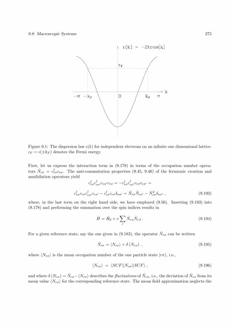
9.8: Macroscopic Systems 275
Figure 9.1: The dispersion law ε(k) for independent electrons on an infinite one dimensional lattice.εF = ε(±kF ) denotes the Fermi energy.
First, let us express the interaction term in (9.178) in terms of the occupation number opera-tors Nrσ = c†rσcrσ. The anti-commutation properties (9.45, 9.46) of the fermionic creation andannihilation operators yield
c†rσc†rσ′crσ′crσ = −c†rσc
†rσ′crσcrσ′ =
c†rσcrσc†rσ′crσ′ − c
†rσcrσδσσ′ = NrσNrσ′ − N2
rσδσσ′ , (9.193)
where, in the last term on the right hand side, we have employed (9.56). Inserting (9.193) into(9.178) and performing the summation over the spin indices results in
H = H0 + v∑r
NrαNrβ . (9.194)
For a given reference state, say the one given in (9.183), the operator Nrσ can be written
Nrσ = 〈Nrσ〉+ δ (Nrσ) , (9.195)
where 〈Nrσ〉 is the mean occupation number of the one particle state |rσ〉, i.e.,
〈Nrσ〉 = 〈SCF ||Nrσ||SCF 〉 , (9.196)
and where δ (Nrσ) = Nrσ−〈Nrσ〉 describes the fluctuations of Nrσ, i.e., the deviation of Nrσ from itsmean value 〈Nrσ〉 for the corresponding reference state. The mean field approximation neglects the
276 Many–Particle Systems
fluctuations to second order and the mean field Hamiltonian is obtained from (9.194) by droppingall the terms which contain the fluctuations to second order. In this approximation one can express
NrαNrβ = (〈Nrα〉+ δ (Nrα)) (〈Nrβ〉+ δ (Nrβ))≈ 〈Nrα〉〈Nrβ〉+ 〈Nrα〉δ (Nrβ) + 〈Nrβ〉δ (Nrα)
= 〈Nrα〉Nrβ + 〈Nrβ〉Nrα − 〈Nrα〉〈Nrβ〉 (9.197)
and the corresponding mean field Hamiltonian becomes
Hmf = H0 + v∑r
(〈Nrα〉Nrβ + 〈Nrβ〉Nrα
)− v
∑r
〈Nrα〉〈Nrβ〉 . (9.198)
Let us assume that the ground state of the Hubbard model, in the mean field approximation, isgiven by (9.183). Because of
〈Nrσ〉 = 〈c†rσcrσ〉 =∑m,m′
UrmU∗rm′〈d†mσdm′σ〉
=N−1∑m=0
UrmU∗rm =
N
2N0=
n
2,
holds
Hmf = H0 +mv
2
∑rσ
c†rσcrσ − 2N0vn2
2
=∑mσ
(εm +
nv
2
)d†mσdmσ −N
vn
2, (9.199)
which is identical to expression (9.191) for the ground state energy. Note that the procedure em-ployed in (9.195), i.e., separating the occupation number operator into a mean value plus fluctuationand neglecting the fluctuations in 2nd order, yields essentially the same mean field Hamiltonian(9.198) as the one obtained by using the mean field potential (9.146).
Spin-Polarized Mean Field Ground State
We want to consider now a ground state for Hmf defined through
〈Nrσ〉 = nσ = const (9.200)
allowing, however, that nα and nβ assume different values. For such state the mean occupationnumber nrσ is uniform at all lattice sites, but the mean number of particles with spin α can bedifferent from the mean number of particles with spin β. Therefore, the ground state of the systemcan have a non-zero local spin and, consequently, non-vanishing magnetization. In case nα = nβthe following construction will lead to a ground state which coincides with the non-magnetic groundstate (9.183) .To determine a magnetic ground state we note
∑r
Nrσ =∑mm′
(∑r
UrmU∗rm′
)d†mσdm′σ =
∑mm′
δmm′Nmσ =∑m
Nmσ ,

9.8: Macroscopic Systems 277
from which we obtainnσ =
12N0
∑m
〈Nmσ〉 . (9.201)
The mean field Hamiltonian is then
Hmf =∑m
[(εm + vnβ) Nmα + (εm + vnα) Nmβ
]− 2N0vnαnβ . (9.202)
This Hamiltonian describes a system of non-interacting electrons with a spin-dependent dispersionlaw
εmσ = εm + vn−σ . (9.203)
The actual values of nσ (σ = α, β) are determined by minimizing the energy density of the groundstate
Emf ≡〈Hmf 〉2N0
=1
2N0
∑m,σ
[εmσ〈Nmσ〉]− vnαnβ (9.204)
with respect to nα and nβ , subject to the constraint
n = nα + nβ . (9.205)
Such minimization is realized through the method of Lagrangian multipliers. According to thismethod one minimizes
Emf = Emf + µ (n− nα − nβ) , (9.206)
where µ is the Lagrangian multiplier considered an independent variable, i.e., Emf is minimizedwith respect to nα, nβ and µ. The additional term in (9.206) ascertains that condition (9.205) ismet.At this point we exploit the fact that our system is macroscopically large, i.e., N0 ∼ 1023. In thislimit the discrete energy spectrum (9.203) is provided by the continuous function
εσ(k) = ε(k) + vn−σ , (9.207)
where ε(k) is given by (9.192). This last equation tells us that the electrons with spin α (β) areaccommodated by an energy sub–band εα(k) (εβ(k)) which is obtained from the dispersion law ofthe non-interactive electrons ε(k) by an overall shift of vnβ (vnα). The ground state (correspondingto the lowest possible energy) of the many electron system is obtained by filling these two energysub–bands with electrons up to the same maximum energy value, the so-called Fermi energy εF = µ(see below), as is shown schematically in Figure 9.2a. Since εβ(k) − εα(k) = v(nα − nβ), one cansee that an uneven occupation by electrons of the two energy bands yields a relative shift of theenergy bands with respect to each other, e.g., if nα > nβ then εβ(k) > εα(k), such that the largernσ, the smaller is εσ(k) for a given k. Therefore, one can expect the system to lower its energy byassuming nα 6= nβ and, hence, a spin–polarized ground state.The values of nα and nβ are determined by minimizing the energy density (9.206). For this purposethe sum in (9.206) needs to be evaluated. In the limit N0 → ∞ this sum can be expressed as anintegral. In fact, for any function f
(mπN0
)holds (compare with the definition of a definite integral
as the limit of the corresponding Riemann sum)
limN0→∞
12N0
N0∑m=−N0+1
f
(mπ
N0
)=∫ π
−π
dk
2πf(k) . (9.208)

278 Many–Particle Systems
(b) (a)
Figure 9.2: (a) Relative position of the two energy sub–bands εα(k) and εβ(k) for ∆ = nα−nβ > 0.The shaded areas represent the filled portions of these bands by electrons. (b) Graphical definitionof the limiting energies εα and εβ.
If the function f depends explicitly only on ε(k) one can state∫ π
−π
dk
2πf (ε(k)) =
∫ ∞−∞
ρ(ε)dεf(ε) (9.209)
whereρ(ε) =
∫ π
−π
dk
2πδ (ε− ε(k)) . (9.210)
Here δ(x) is the Dirac–delta function and ρ(ε), which is usually called the density of states, givesthe the number of available one particle states per site, unit energy and a given spin orientation ofthe particle.For a given dispersion law ε(k) the density of states ρ(ε) can be calculated by employing equation(9.210). In our case ε(k) is given by (9.192) and, therefore, holds
ρ(ε) =∫ π
−π
dk
2πδ(ε+ 2t cos k) . (9.211)
In order to calculate the integral we recall the following property of the Dirac–delta function
δ [f(x)] =∑i
δ(x− xi)|f ′(xi)|
, (9.212)
where xi are the simple roots of the function f(x). Since the equation f(k) ≡ 2t cos k + ε = 0 hastwo simple roots, namely k1,2 = ±(π − arccos(ε/2t)), and noting
|f ′(k)| = |2t sin k| = 2t√
1− cos2 k =√
(2t)2 − ε2 ,
one obtainsδ(ε− ε(k)) =
δ(k + π − arccos(ε/2t)) + δ(k − π + arccos(ε/2t))√(2t)2 − ε2
.
Inserting this last result into (9.211) and using∫ π
−πdkδ(k ± (π − arccos(ε/2t))) = θ(2t− |ε|) ,
9.8: Macroscopic Systems 279
where θ(x) is the step function, i.e., θ(x) = 1 if x > 0 and θ(x) = 0 if x < 0, one arrives at thefollowing expression of the density of states
ρ(ε) =θ(2t− |ε|)
π√
(2t)2 − ε2. (9.213)
The presence of the θ function in the above formula guaranties that the density of states vanishesfor |ε| > 2t, i.e., outside the energy band ε(k); if we assume that ε is restricted to the interval]− 2t, 2t[ then the θ function in (9.213) can simply be replaced by 1.We can employ the results obtained to express the ground state energy density (9.204) through anintegral expression. One obtains
Emf =∫ εα
−2tερ(ε)dε+
∫ εβ
−2tερ(ε)dε+ vnαnβ + µ(n− nα − nβ) , (9.214)
where εσ denotes the value of ε(k) which corresponds to the top of the filled portion of the energysub–band εσ(k) [c.f. Fig. 9.2], i.e.,
εF = εα + vnβ = εβ + vnα . (9.215)
nα and nβ in (9.214) are given by the sum (9.201). Replacing again the sum by an integral overenergy one can write
nσ =∫ εσ
−2tρ(ε)dε (9.216)
Using (9.213) and carrying out the resulting integral yields
nσ =1π
arcsin(εσ/2t) . (9.217)
Since Emf [c.f. (9.206)] depends only on continuous quantities, namely, on εα, εβ and µ, the necessaryconditions for a ground state of minimum energy are
∂Emf∂εα
= 0 ,∂Emf∂εβ
= 0 ,∂Emf∂µ
= 0 . (9.218)
The derivatives can be readily determined and the conditions (9.218) read
∂Emf∂εα
= εα + vnβ − µ = 0 , (9.219)
∂Emf∂εβ
= εβ + vnα − µ = 0 , (9.220)
and∂Emf∂µ
= n− nα − nβ = 0 . (9.221)
Equations (9.219–9.221) and (9.216) allow one, in principle, to determine the unknown quantitiesεα, εβ, µ, nα and nβ as a function of the parameters of the Hubbard model, namely, of t, v and n.From (9.219, 9.220) µ can be readily obtained
µ =12
(εα + εβ) +vn
2, (9.222)
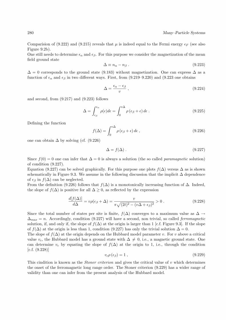
280 Many–Particle Systems
Comparision of (9.222) and (9.215) reveals that µ is indeed equal to the Fermi energy εF (see alsoFigure 9.2b).One still needs to determine εα and εβ . For this purpose we consider the magnetization of the meanfield ground state
∆ ≡ nα − nβ . (9.223)
∆ = 0 corresponds to the ground state (9.183) without magnetization. One can express ∆ as afunction of εα and εβ in two different ways. First, from (9.219–9.220) and (9.223 one obtains
∆ =εα − εβv
, (9.224)
and second, from (9.217) and (9.223) follows
∆ =∫ εα
εβ
ρ(ε)dε =∫ v∆
0ρ (εβ + ε) dε . (9.225)
Defining the function
f(∆) =∫ v∆
0ρ (εβ + ε) dε , (9.226)
one can obtain ∆ by solving (cf. (9.226)
∆ = f(∆) . (9.227)
Since f(0) = 0 one can infer that ∆ = 0 is always a solution (the so called paramagnetic solution)of condition (9.227).Equation (9.227) can be solved graphically. For this purpose one plots f(∆) versus ∆ as is shownschematically in Figure 9.3. We assume in the following discussion that the implicit ∆ dependenceof εβ in f(∆) can be neglected.From the definition (9.226) follows that f(∆) is a monotonically increasing function of ∆. Indeed,the slope of f(∆) is positive for all ∆ ≥ 0, as reflected by the expression
d[f(∆)]d∆
= vρ(εβ + ∆) =v
π√
(2t)2 − (v∆ + εβ)2> 0 . (9.228)
Since the total number of states per site is finite, f(∆) converges to a maximum value as ∆ →∆max = n. Accordingly, condition (9.227) will have a second, non trivial, so called ferromagneticsolution, if, and only if, the slope of f(∆) at the origin is larger than 1 [c.f. Figure 9.3]. If the slopeof f(∆) at the origin is less than 1, condition (9.227) has only the trivial solution ∆ = 0.The slope of f(∆) at the origin depends on the Hubbard model parameter v. For v above a criticalvalue vc, the Hubbard model has a ground state with ∆ 6= 0, i.e., a magnetic ground state. Onecan determine vc by equating the slope of f(∆) at the origin to 1, i.e., through the condition[c.f. (9.228)]
vcρ (εβ) = 1 , (9.229)
This cindition is known as the Stoner criterion and gives the critical value of v which determinesthe onset of the ferromagnetic long range order. The Stoner criterion (9.229) has a wider range ofvalidity than one can infer from the present analysis of the Hubbard model.
9.8: Macroscopic Systems 281
Figure 9.3: Graphical solution of the mean field equation ∆ = f(∆).
By parameterizing εα and εβεα = 2t sinx , εβ = 2t sin y , (9.230)
one obtains from (9.219, 9.220, 9.205) the following set of equations determining x, y and, hence,εα, εβ
x+ y = π(n− 1) (9.231)
x− y = π2tv
(sinx− sin y) = π∆ . (9.232)
For a given 2tv the values of x and y can be obtained numerically and other relevant quantities
mentioned above can be calculated.We like to determine finally the dependence of vc
2t on the filling factor n. The correspondinganalytical expression provides the phase diagram of the ground state: when v approaches vc fromabove, the magnetization ∆ of the ground state vanishes and remains zero for values v < vc.Equation (9.232) states that x − y is proportional to ∆. Since ∆ vanishes near vc we set x = y+ δwhere δ is a small quantity. From (9.231) follows
y =π
2(n− 1)− δ
2≈ π
2(n− 1) . (9.233)
Employing the approximation sin(y + δ)− sin y ≈ δ cos y for small δ, (9.232) together with (9.233)yield the desired expression
vc2t
= π cos[π
2(n− 1)
]. (9.234)
The resulting phase diagram of the ground state, i.e., the plot of vc2t vs. n, is presented in Figure 9.4.As already mentioned, the ground state is characterized by the quantities (v, t, n). Accordingly, any

282 Many–Particle Systems
mean field ground state is represented by a point in the phase diagram. The magnetic nature of theground state of the system depends on whether the representative point lies inside the ferromagneticor inside the paramagnetic domain of the phase diagram.
Figure 9.4: Ground state phase diagram of the mean field Hamiltonian (9.202).
Concluding Remarks
At the end of our analysis of the mean field ground state of the one-dimensional Hubbard model,it is natural to ask oneself if the results obtained reflect, at least qualitatively, the properties ofthe real ground state of the Hubbard model. Well, the answer is no. The real ground state ofthe one-dimensional Hubbard model is quite different in nature from the mean field ground statediscussed here. The reason is that the effect of quantum fluctuations, which are neglected in themean field theory, in one spatial dimension is very strong.Nevertheless, the analysis presented above is not quite useless. First, once we specify a class ofpossible states to which the real ground state might belong to, the method described above givesa systematic way of singling out the state with the lowest possible energy which might be a goodcandidate for the real ground state of the system. Second, since in one spatial dimension there aremany exact results available, the application of the mean field theory for these systems provides anexcellent testing opportunity of these theories by comparing their predicted results with the exactones. Third, the mean field theory of the one-dimensional Hubbard model can be extended in astraightforward way to higher spatial dimensions. In general, the effect of quantum fluctuations isgetting less important as the dimensionality of the system is increased. For example, in three spatialdimensions the theory presented above works fine in the case of the transitional–metal oxides suchas NiO and CoO. However, strong electron correlation effects , even in these materials, can lead toserious modifications of the mean field ground state.
9.8: Macroscopic Systems 283
In case of two spatial dimensions things are more complicated. On the one hand, the lack of exactsolutions, and on the other hand, the strong effect of quantum fluctuations of the strongly correlatedelectron system described by the Hubbard Hamiltonian makes all the presently existing solutionsquestionable. In fact, in the case of the copper oxide high temperature superconductors, whichinvolve strongly correlated quasi two-dimensional electron systems, a reliable microscopic theory isstill lacking. The available mean field theories cannot account for all the striking, unusual physicalproperties of these materials.

284 Many–Particle Systems

Chapter 10
Relativistic Quantum Mechanics
In this Chapter we will address the issue that the laws of physics must be formulated in a formwhich is Lorentz–invariant, i.e., the description should not allow one to differentiate between framesof reference which are moving relative to each other with a constant uniform velocity ~v. Thetransformations beween such frames according to the Theory of Special Relativity are describedby Lorentz transformations. In case that ~v is oriented along the x1–axis, i.e., ~v = v1x1, thesetransformations are
x1′ =x1 − v1t√1 −
(v1c
)2 , t′ =t − v1
c2x1√
1 −(v1c
)2 , x′2 = x2 ; x′3 = x3 (10.1)
which connect space time coordinates (x1, x2, x3, t) in one frame with space time coordinates(x′1, x
′2, x′3, t′) in another frame. Here c denotes the velocity of light. We will introduce below
Lorentz-invariant differential equations which take the place of the Schrodinger equation of a par-ticle of mass m and charge q in an electromagnetic field [c.f. (refeq:ham2, 8.45)] described by anelectrical potential V (~r, t) and a vector potential ~A(~r, t)
i~∂
∂tψ(~r, t) =
[1
2m
(~
i∇ − q
c~A(~r, t)
)2
+ qV (~r, t)]ψ(~r, t) (10.2)
The replacement of (10.2) by Lorentz–invariant equations will have two surprising and extremelyimportant consequences: some of the equations need to be formulated in a representation for whichthe wave functions ψ(~r, t) are vectors of dimension larger one, the components representing thespin attribute of particles and also representing together with a particle its anti-particle. We willfind that actually several Lorentz–invariant equations which replace (10.2) will result, any of theseequations being specific for certain classes of particles, e.g., spin–0 particles, spin–1
2 particles, etc.As mentioned, some of the equations describe a particle together with its anti-particle. It is notpossible to uncouple the equations to describe only a single type particle without affecting nega-tively the Lorentz invariance of the equations. Furthermore, the equations need to be interpretedas actually describing many–particle-systems: the equivalence of mass and energy in relativisticformulations of physics allows that energy converts into particles such that any particle describedwill have ‘companions’ which assume at least a virtual existence.Obviously, it will be necessary to begin this Chapter with an investigation of the group of Lorentztransformations and their representation in the space of position ~r and time t. The representation
285

286 Relativistic Quantum Mechanics
in Sect. 10.1 will be extended in Sect. 10.4 to cover fields, i.e., wave functions ψ(~r, t) and vectorswith functions ψ(~r, t) as components. This will provide us with a general set of Lorentz–invariantequations which for various particles take the place of the Schrodinger equation. Before introduc-ing these general Lorentz–invariant field equations we will provide in Sects. 10.5, 10.7 a heuristicderivation of the two most widely used and best known Lorentz–invariant field equations, namelythe Klein–Gordon (Sect. 10.5) and the Dirac (Sect. 10.7) equation.
10.1 Natural Representation of the Lorentz Group
In this Section we consider the natural representation of the Lorentz group L, i.e. the group ofLorentz transformations (10.1). Rather than starting from (10.1), however, we will provide a morebasic definition of the transformations. We will find that this definition will lead us back to thetransformation law (10.1), but in a setting of representation theory methods as applied in Secti. 5to the groups SO(3) and SU(2) of rotation transformations of space coordinates and of spin.The elements L ∈ L act on 4–dimensional vectors of position– and time–coordinates. We willdenote these vectors as follows
xµdef= (x0, x1, x2, x3) (10.3)
where x0 = ct describes the time coordinate and (x1, x2, x3) = ~r describes the space coordinates.Note that the components of xµ all have the same dimension, namely that of length. We will,henceforth, assume new units for time such that the velocity of light c becomes c = 1. This choiceimplies dim(time) = dim(length).
Minkowski Space
Historically, the Lorentz transformations were formulated in a space in which the time componentof xµ was chosen as a purely imaginary number and the space components real. This space iscalled the Minkowski space. The reason for this choice is that the transformations (10.1) leave thequantity
s2 = (x0)2 − (x1)2 − (x2)2 − (x3)2 (10.4)
invariant, i.e., for the transformed space-time–cordinates x′µ = (x′0, x′1, x′2, x′3) holds
(x0)2 − (x1)2 − (x2)2 − (x3)2 = (x′0)2 − (x′1)2 − (x′2)2 − (x′3)2 . (10.5)
One can interprete the quantity√−s2 as a distance in a 4–dimensional Euclidean space if one
chooses the time component purely imaginary. In such a space Lorentz transformations corre-spond to 4-dimensional rotations. Rather than following this avenue we will introduce Lorentztransformations within a setting which does not require real and imaginary coordinates.
The Group of Lorentz Transformations L = O(3,1)
The Lorentz transformations L describe the relationship between space-time coordinates xµ of tworeference frames which move relative to each other with uniform fixed velocity ~v and which mightbe reoriented relative to each other by a rotation around a common origin. Denoting by xµ the

10.1: Natural Representation of the Lorentz Group 287
coordinates in one reference frame and by x′µ the coordinates in the other reference frame, theLorentz transformations constitute a linear transformation which we denote by
x′µ =
3∑ν=0
Lµνxν . (10.6)
Here Lµν are the elements of a 4 × 4–matrix representing the Lorentz transformation. The upperindex closer to ‘L’ denotes the first index of the matrix and the lower index ν further away from‘L’ denotes the second index. [ A more conventional notation would be Lµν , however, the latternotation will be used for different quantities further below.] The following possibilities exist for thepositioning of the indices µ, ν = 0, 1, 2, 3:
4-vector: xµ, xµ ; 4× 4 tensor: Aµν , Aµν , Aµν , Aµν . (10.7)
The reason for the notation is two-fold. First, the notation in (10.6) allows us to introduce theso-called summation conventon: any time the same index appears in an upper and a lower position,summation over that index is assumed without explicitly noting it, i.e.,
yµxµ︸ ︷︷ ︸
new
=3∑
µ=0
yµxµ
︸ ︷︷ ︸old
; Aµνxν︸ ︷︷ ︸new
=3∑
ν=0
Aµνxν
︸ ︷︷ ︸old
; AµνBνρ︸ ︷︷ ︸
new
=3∑
ν=0
AµνBνρ︸ ︷︷ ︸
old
. (10.8)
The summation convention allows us to write (10.6) x′µ = Lµνxν . The second reason is that upper
and lower positions allow us to accomodate the expression (10.5) into scalar products. This will beexplained further below.The Lorentz transformations are non-singular 4× 4–matrices with real coefficients, i.e., L ∈GL(4,R), the latter set constituting a group. The Lorentz transformations form the subgroup of allmatrices which leave the expression (10.5) invariant. This condition can be written
xµgµνxν = x′
µgµνx
′ν (10.9)
where
( gµν ) =
1 0 00 −1 0 00 0 −1 00 0 0 −1
= g . (10.10)
Combining condition (10.9) and (10.6) yields
LµρgµνLνσ x
ρxσ = gρσ xρxσ . (10.11)
Since this holds for any xµ it must be true
LµρgµνLνσ = gρσ . (10.12)
This condition specifies the key property of Lorentz transformations. We will exploit this propertybelow to determine the general form of the Lorentz transformations. The subset of GL(4, R), the
288 Relativistic Quantum Mechanics
elements of which satisfy this condition, is called O(3,1). This set is identical with the set of allLorentz transformations L. We want to show now L = O(3,1) ⊂ GL(4, R) is a group.To simplify the following proof of the key group properties we like to adopt the conventional matrixnotation for Lµν
L = (Lµν ) =
L0
0 L01 L0
2 L03
L10 L1
1 L12 L1
3
L20 L2
1 L22 L3
3
L30 L3
1 L32 L3
3
. (10.13)
Using the definition (10.10) of g one can rewrite the invariance property (10.12)
LT gL = g . (10.14)
From this one can obtain usingg2 = 11 (10.15)
(gLTg)L = 11 and, hence, the inverse of L
L−1 = g LT g =
L0
0 −L10 −L2
0 −L30
−L01 L1
1 L21 L3
1
−L02 L1
2 L22 L3
2
−L03 L1
3 L23 L3
3
. (10.16)
The corresponding expression for (LT )−1 is obviously
(LT )−1 = (L−1)T = g L g . (10.17)
To demonstrate the group property of O(3,1), i.e., of
O(3, 1) = L,L ∈ GL(4,R), LTgL = g , (10.18)
we note first that the identity matrix 11 is an element of O(3,1) since it satisfies (10.14). We considerthen L1,L2 ∈ O(3,1). For L3 = L1L2 holds
LT3 g L3 = LT2 LT1 g L1L2 = LT2 (LT1 gL1) L2 = LT2 g L2 = g , (10.19)
i.e., L3 ∈ O(3,1). One can also show that if L ∈ O(3,1), the associated inverse obeys (10.14), i.e.,L−1 ∈ O(3,1). In fact, employing expressions (10.16, 10.17) one obtains
(L−1)T g L−1 = gLgggLTg = gLgLTg . (10.20)
Multiplying (10.14) from the right by gLT and using (10.15) one can derive LTgLgLT = LT andmultiplying this from the left by by g(LT )−1 yields
L g LT = g (10.21)
Using this result to simplify the r.h.s. of (10.20) results in the desired property
(L−1)T g L−1 = g , (10.22)
i.e., property (10.14) holds for the inverse of L. This stipulates that O(3,1) is, in fact, a group.

10.1: Natural Representation of the Lorentz Group 289
Classification of Lorentz Transformations
We like to classify now the elements of L = O(3,1). For this purpose we consider first the valueof detL. A statement on this value can be made on account of property (10.14). Using detAB =detAdetB and detAT = detA yields (detL)2 = 1 or
detL = ±1 . (10.23)
One can classify Lorentz transformations according to the value of the determinant into two distinctclasses.A second class property follows from (10.14) which we employ in the formulation (10.12). Consid-ering in (10.12) the case ρ = 0, σ = 0 yields(
L00
)2 − (L1
0
)2 − (L2
0
)2 − (L3
0
)2 = 1 . (10.24)
or since (L10)2 + (L2
0)2 + (L30)2 ≥ 0 it holds (L0
0)2 ≥ 1. From this we can conclude
L00 ≥ 1 or L0
0 ≤ −1 , (10.25)
i.e., there exist two other distinct classes. Properties (10.23) and (10.25) can be stated as follows:The set of all Lorentz transformations L is given as the union
L = L↑+ ∪ L↓+ ∪ L
↑− ∪ L
↓− (10.26)
where L↑+, L↓+, L
↑−, L
↓− are disjunct sets defined as follows
L↑+ = L,L ∈ O(3, 1), detL = 1, L00 ≥ 1 ; (10.27)
L↓+ = L,L ∈ O(3, 1), detL = 1, L00 ≤ −1 ; (10.28)
L↑− = L,L ∈ O(3, 1), detL = −1, L00 ≥ 1 ; (10.29)
L↓− = L,L ∈ O(3, 1), detL = −1, L00 ≤ −1 . (10.30)
It holds g ∈ L and −11 ∈ L as one can readily verify testing for property (10.14). One can alsoverify that one can write
L↑− = gL↑+ = L↑+g ; (10.31)
L↓+ = −L↑+ ; (10.32)
L↓− = −gL↑+ = −L↑+g (10.33)
where we used the definition aM = M1,∃M2,M2 ∈ M,M1 = aM2. The above shows thatthe set of proper Lorentz transformations L↑+ allows one to generate all Lorentz transformations,except for the trivial factors g and −11. It is, hence, entirely suitable to investigate first onlyLorentz transformations in L↑+.We start our investigation by demonstrating that L↑+ forms a group. Obviously, L↑+ contains 11.We can also demonstrate that for A,B ∈ L↑+ holds C = AB ∈ L↑+. For this purpose we considerthe value of C0
0 = A0µB
µ0 =
∑3j=1A
0jB
j0 + A0
0B0
0. Schwartz’s inequality yields 3∑j=1
A0jB
j0
2
≤3∑j=1
(A0
j
)2 3∑j=1
(Bj
0
)2. (10.34)

290 Relativistic Quantum Mechanics
From (10.12) follows (B00)2 −
∑3j=1(Bj
0)2 = 1 or∑3
j=1(Bj0)2 = (B0
0)2 − 1. Similarly, one canconclude from (10.21)
∑3j=1(A0
j)2 = (A00)2 − 1. (10.34) provides then the estimate 3∑
j=1
A0jB
j0
2
≤[
(A00)2 − 1
] [(B0
0)2 − 1]< (A0
0)2 (B00)2 . (10.35)
One can conclude, therefore, |∑3
j=1A0jB
j0| < A0
0B0
0. Since A00 ≥ 1 and B0
0 ≥ 1, obviouslyA0
0B0
0 ≥ 1. Using the above expression for C00 one can state C0
0 > 0. In fact, since the groupproperty of O(3,1) ascertains CTgC = g it must hold C0
0 ≥ 1.The next group property of L↑+ to be demonstrated is the existence of the inverse. For the inverse ofany L ∈ L↑+ holds (10.16). This relationship shows (L−1)0
0 = L00, from which one can conclude
L−1 ∈ L↑+. We also note that the identity operator 11 has elements
11µν = δµν (10.36)
where we defined1
δµν =
1 for µ = ν0 for µ 6= ν
(10.37)
It holds, 1100 =≥ 1 and, hence, 11 ∈ L↑+. Since the associative property holds for matrix multipli-
cation we have verified that L↑+ is indeed a subgroup of SO(3,1).L↑+ is called the subgroup of proper, orthochronous Lorentz transformations. In the following wewill consider solely this subgroup of SO(3,1).
Infinitesimal Lorentz transformations
The transformations in L↑+ have the property that they are continously connected to the identity 11,i.e., these transformations can be parametrized such that a continuous variation of the parametersconnects any element of L↑+ with 11. This property will be exploited now in that we consider firsttransformations in a small neighborhood of 11 which we parametrize by infinitesimal parameters.We will then employ the Lie group properties to generate all transformations in L↑+.Accordingly, we consider transformations
Lµν = δµν + εµν ; εµν small . (10.38)
For these transformations, obviously, holds L00 > 0 and the value of the determinant is close to
unity, i.e., if we enforce (10.14) actually L00 ≥ 1 and det L = 1 must hold. Property (10.14)
implies (11 + εT
)g ( 11 + ε ) = g (10.39)
where we have employed the matrix form ε defined as in (10.13). To order O(ε2) holds
εT g + g ε = 0 . (10.40)1It should be noted that according to our present definition holds δµν = gµρδ
ρν and, accordingly, δ00 = 1 and
δ11 = δ22 = δ33 = −1.

10.1: Natural Representation of the Lorentz Group 291
Using (10.15) one can concludeεT = −g εg (10.41)
which reads explicitlyε00 ε10 ε20 ε30
ε01 ε11 ε21 ε31
ε02 ε12 ε22 ε32
ε03 ε13 ε23 ε33
=
−ε00 ε01 ε02 ε03
ε10 −ε11 −ε12 −ε13
ε20 −ε21 −ε22 −ε23
ε30 −ε31 −ε32 −ε33
. (10.42)
This relationship implies
εµµ = 0ε0j = εj0 , j = 1, 2, 3εjk = − εkj , j, k = 1, 2, 3 (10.43)
Inspection shows that the matrix ε has 6 independent elements and can be written
ε(ϑ1, ϑ2, ϑ3, w1, w2, w3) =
0 −w1 −w2 −w3
−w1 0 −ϑ3 ϑ2
−w2 ϑ3 0 −ϑ1
−w3 −ϑ2 ϑ1 0
. (10.44)
This result allows us now to define six generators for the Lorentz transformations(k = 1, 2, 3)
Jk = ε(ϑk = 1, other five parameters zero) (10.45)
Kk = ε(wk = 1, other five parameters zero) . (10.46)
The generators are explicitly
J1 =
0 0 0 00 0 0 00 0 0 −10 0 1 0
; J2 =
0 0 0 00 0 0 10 0 0 00 −1 0 0
; J3 =
0 0 0 00 0 −1 00 1 0 00 0 0 0
(10.47)
K1 =
0 −1 0 0−1 0 0 0
0 0 0 00 0 0 0
; K2 =
0 0 −1 00 0 0 0−1 0 0 0
0 0 0 0
; K3 =
0 0 0 −10 0 0 00 0 0 0−1 0 0 0
(10.48)
These commutators obey the following commutation relationships
[ Jk, J` ] = εk`m Jm (10.49)[ Kk, K` ] = − εk`m Jm[ Jk, K` ] = εk`m Km .
The operators also obey~J · ~K = J1J1 + J2J2 + J3J3 = 0 (10.50)
292 Relativistic Quantum Mechanics
as can be readily verified.
Exercise 7.1:Demonstrate the commutation relationships (10.49, 10.50).
The commutation relationships (10.49) define the Lie algebra associated with the Lie group L↑+.The commutation relationships imply that the algebra of the generators Jk, Kk, k = 1, 2, 3 is closed.Following the treatment of the rotation group SO(3) one can express the elements of L↑+ throughthe exponential operators
L(~ϑ, ~w) = exp(~ϑ · ~J + ~w · ~K
); ~ϑ, ~w ∈ R3 (10.51)
where we have defined ~ϑ · ~J =∑3
k=1 ϑkJk and ~w · ~K =∑3
k=1wkKk. One can readily show,following the algebra in Chapter 5, and using the relationship
Jk =(
0 00 Lk
)(10.52)
where the 3 × 3–matrices Lk are the generators of SO(3) defined in Chapter 5, that the transfor-mations (10.51) for ~w = 0 correspond to rotations of the spatial coordinates, i.e.,
L(~ϑ, ~w = 0) =(
0 00 R(~ϑ)
). (10.53)
Here R(~ϑ) are the 3× 3–rotation matrices constructed in Chapter 5. For the parameters ϑk of theLorentz transformations holds obviously
ϑk ∈ [0, 2π[ , k = 1, 2, 3 (10.54)
which, however, constitutes an overcomplete parametrization of the rotations (see Chapter 5).We consider now the Lorentz transformations for ~ϑ = 0 which are referred to as ‘boosts’. A boostin the x1–direction is L = exp(w1K1). To determine the explicit form of this transformation weevaluate the exponential operator by Taylor expansion. In analogy to equation (5.35) it issufficientto consider in the present case the 2× 2–matrix
L′ = exp(w1
(0 −1−1 0
))=
∞∑n=0
wn1n!
(0 −1−1 0
)n(10.55)
since
exp (w1K1) = exp
L′0 00 0
0 00 0
1 00 1
. (10.56)
Using the idempotence property(0 −1−1 0
)2
=(
1 00 1
)= 11 (10.57)
10.1: Natural Representation of the Lorentz Group 293
one can carry out the Taylor expansion above:
L′ =∞∑n=0
w2n1
(2n)!11 +
∞∑n=0
w2n+11
(2n+ 1)!
(0 −1−1 0
)(10.58)
= coshw1 11 + sinhw1
(0 −1−1 0
)=(
coshw1 −sinhw1
−sinhw1 coshw1
).
The conventional form (10.1) of the Lorentz transformations is obtained through the parameterchange
v1 =sinhw1
coshw1= tanhw1 (10.59)
Using cosh2w1 − sinh2w1 = 1 one can identify sinhw1 =√
cosh2w1 − 1 and coshw1 =√sinh2w1 + 1. Correspondingly, one obtains from (10.59)
v1 =
√cosh2w1 − 1
coshw1=
sinhw1√sinh2w1 + 1
. (10.60)
These two equations yield
coshw1 = 1/√
1− v21 ; sinhw1 = v1/
√1− v2
1 , (10.61)
and (10.56, 10.59) can be written
exp (w1K1) =
1√
1− v21
−v1√1− v2
1
0 0−v1√1− v2
1
1√1− v2
1
0 0
0 0 1 00 0 0 1
(10.62)
According to (10.3, 10.6, 10.51) the explicit transformation for space–time–coordinates is then
x′1 =x1 − v1t√
1 − v21
, t′ =t − v1x1√
1 − v21
, x′2 = x2 , x′3 = x3 (10.63)
which agrees with (10.1).The range of the parameters wk can now be specified. vk defined in (10.59) for the case k = 1corresponds to the relative velocity of two frames of reference. We expect that vk can only assumevalues less than the velocity of light c which in the present units is c = 1. Accordingly, we canstate vk ∈ ]−1, 1[. This property is, in fact, consistent with (10.59). From (10.59) follows, however,for wk
wk ∈ ]−∞, ∞[ . (10.64)
We note that the range of wk-values is not a compact set even though the range of vk-values iscompact. This property of the wk-values contrasts with the property of the parameters ϑk specifyingrotational angles which assume only values in a compact range.

294 Relativistic Quantum Mechanics
10.2 Scalars, 4–Vectors and Tensors
In this Section we define quantities according to their behaviour under Lorentz transformations.Such quantities appear in the description of physical systems and statements about transformationproperties are often extremely helpful and usually provide important physical insight. We haveencountered examples in connection with rotational transformations, namely, scalars like r =√x2
1 + x22 + x2
3, vectors like ~r = (x1, x2, x3)T , spherical harmonics Y`m(r), total angular momentumstates of composite systems like Y`m(`1, `2|r1, r2) and, finally, tensor operators Tkm. Some of thesequantities were actually defined with respect to representations of the rotation group in functionspaces, not in the so-called natural representation associated with the 3–dimensional Euclideanspace E3.Presently, we have not yet defined representations of Lorentz transformations beyond the ‘natural’representation acting in the 4–dimensional space of position– and time–coordinates. Hence, ourdefinition of quantities with special properties under Lorentz transformations presently is confinedto the natural representation. Nevertheless, we will encounter an impressive example of physicalproperties.
Scalars The quantities with the simplest transformation behaviour are so-called scalars f ∈ Rwhich are invariant under transformations, i.e.,
f ′ = f . (10.65)
An example is s2 defined in (10.4), another example is the rest mass m of a particle. However, notany physical property f ∈ R is a scalar. Counterexamples are the energy, the charge density, thez–component x3 of a particle, the square of the electric field | ~E(~r, t)|2 or the scalar product ~r1 · ~r2
of two particle positions. We will see below how true scalars under Lorentz transformations can beconstructed.
4-Vectors The quantities with the transformation behaviour like that of the position–time vectorxµ defined in (10.3) are the so-called 4–vectors aµ. These quantites always come as four components(a0, a1, a2, a3)T and transform according to
a′µ = Lµνa
ν . (10.66)
Examples of 4-vectors beside xµ are the momentum 4-vector
pµ = (E, ~p) , E =m√
1 − ~v 2, ~p =
m~v√1 − ~v 2
(10.67)
the transformation behaviour of which we will demonstrate further below. A third 4-vector is theso-called current vector
Jµ = (ρ, ~J) (10.68)
where ρ(~r, t) and ~J(~r, t) are the charge density and the current density, respectively, of a system ofcharges. Another example is the potential 4-vector
Aµ = (V, ~A) (10.69)
where V (~r, t) and ~A(~r, t) are the electrical and the vector potential of an electromagnetic field. The4-vector character of Jµ and of Aµ will be demonstrated further below.
10.2: Scalars, 4–Vectors and Tensors 295
Scalar Product 4-vectors allow one to construct scalar quantities. If aµ and bµ are 4-vectorsthen
aµgµνbν (10.70)
is a scalar. This property follows from (10.66) together with (10.12)
a′µgµνb
′ν = LµρgµνLνσa
ρbσ = aρgρσbσ (10.71)
Contravariant and Covariant 4-Vectors It is convenient to define a second class of 4-vectors.The respective vectors aµ are associated with the 4-vectors aµ, the relationship being
aµ = gµνaν = (a0,−a1,−a2,−a3) (10.72)
where aν is a vector with transformation behaviour as stated in (10.66). One calls 4-vectors aµcovariant and 4-vectors aµ contravariant. Covariant 4-vectors transform like
a′µ = gµνLνρgρσaσ (10.73)
where we definedgµν = gµν . (10.74)
We like to point out that from definition (10.72) of the covariant 4-vector follows aµ = gµνaν . Infact, one can employ the tensors gµν and gµν to raise and lower indices of Lµν as well. We do notestablish here the consistency of the ensuing notation. In any case one can express (10.73)
a′µ = Lµσaσ . (10.75)
Note that according to (10.17) Lµσ is the transformation inverse to Lσµ. In fact, one can express[(L−1)T ]µν = (L−1)νµ and, accordingly, (10.17) can be written
(L−1)νµ = Lµν . (10.76)
The 4-Vector ∂µ An important example of a covariant 4-vector is the differential operator
∂µ =∂
∂xµ=(∂
∂t, ∇)
(10.77)
The transformed differential operator will be denoted by
∂′µdef=
∂
∂x′µ. (10.78)
To prove the 4-vector property of ∂µ we will show that gµν∂ν transforms like a contravariant 4-vector, i.e., gµν∂′ν = Lµρg
ρσ∂σ. We start from x′µ = Lµνxν . Multiplication (and summation) of
x′µ = Lµνxν by Lρσgρµ yields, using (10.12), gσνxν = Lρσgρµx
′µ and gµσgσν = δµν ,
xν = gνσLρσgρµx′µ . (10.79)
This is the inverse Lorentz transformation consistent with (10.16). We have duplicated the expres-sion for the inverse of Lµν to obtain the correct notation in terms of covariant, i.e., lower, and
296 Relativistic Quantum Mechanics
contravariant, i.e., upper, indices. (10.79) allows us to determine the connection between ∂µ and∂′µ. Using the chain rule of differential calculus we obtain
∂′µ =3∑
ν=0
∂xν
∂x′µ∂
∂xν= gνσLρσgρµ∂ν = Lµ
ν ∂ν (10.80)
Multiplication by gλµ (and summation over µ) together with gλµgρµ = δλρ yields
gλµ∂′µ = Lλσgσν∂ν , (10.81)
i.e., ∂µ does indeed transform like a covariant vector.
d’Alembert Operator We want to construct now a scalar differential operator. For this purposewe define first the contravariant differential operator
∂µ = gµν∂ν =(∂
∂t, −∇
). (10.82)
Then the operator∂µ∂
µ = ∂2t − ∇2 (10.83)
is a scalar under Lorentz transformations. In fact, this operator is equal to the d’Alembert operatorwhich is known to be Lorentz-invariant.
Proof that pµ is a 4-vector We will demonstrate now that the momentum 4-vector pµ definedin (10.67) transforms like (10.66). For this purpose we consider the scalar differential
(dτ)2 = dxµdxµ = (dt)2 − (d~r)2 (10.84)
It holds (dτ
dt
)2
= 1 − (~v)2 (10.85)
from which followsd
dτ=
1√1 − ~v 2
d
dt. (10.86)
One can writep0 = E =
m√1 − ~v 2
=m√
1 − ~v 2
dt
dt. (10.87)
The remaining components of pµ can be written, e.g.,
p1 =mv1
√1 − ~v 2
=m√
1 − ~v 2
dx1
dt. (10.88)
One can express then the momentum vector
pµ =m√
1 − ~v 2
dxµ
dt= m
d
dτxµ . (10.89)
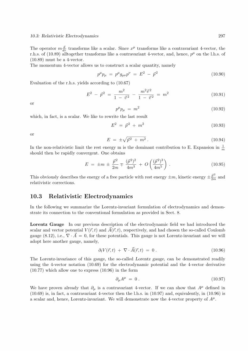
10.3: Relativistic Electrodynamics 297
The operator m ddτ transforms like a scalar. Since xµ transforms like a contravariant 4-vector, the
r.h.s. of (10.89) alltogether transforms like a contravariant 4-vector, and, hence, pµ on the l.h.s. of(10.89) must be a 4-vector.The momentum 4-vector allows us to construct a scalar quantity, namely
pµpµ = pµgµνpν = E2 − ~p 2 (10.90)
Evaluation of the r.h.s. yields according to (10.67)
E2 − ~p 2 =m2
1 − ~v 2− m2~v 2
1 − ~v 2= m2 (10.91)
orpµpµ = m2 (10.92)
which, in fact, is a scalar. We like to rewrite the last result
E2 = ~p 2 + m2 (10.93)
orE = ±
√~p 2 + m2 . (10.94)
In the non-relativistic limit the rest energy m is the dominant contribution to E. Expansion in 1m
should then be rapidly convergent. One obtains
E = ±m ± ~p 2
2m∓ (~p 2)2
4m3+ O
((~p 2)3
4m5
). (10.95)
This obviously describes the energy of a free particle with rest energy ±m, kinetic energy ± ~p 2
2m andrelativistic corrections.
10.3 Relativistic Electrodynamics
In the following we summarize the Lorentz-invariant formulation of electrodynamics and demon-strate its connection to the conventional formulation as provided in Sect. 8.
Lorentz Gauge In our previous description of the electrodynamic field we had introduced thescalar and vector potential V (~r, t) and ~A(~r, t), respectively, and had chosen the so-called Coulombgauge (8.12), i.e., ∇ · ~A = 0, for these potentials. This gauge is not Lorentz-invariant and we willadopt here another gauge, namely,
∂tV (~r, t) + ∇ · ~A(~r, t) = 0 . (10.96)
The Lorentz-invariance of this gauge, the so-called Lorentz gauge, can be demonstrated readilyusing the 4-vector notation (10.69) for the electrodynamic potential and the 4-vector derivative(10.77) which allow one to express (10.96) in the form
∂µAµ = 0 . (10.97)
We have proven already that ∂µ is a contravariant 4-vector. If we can show that Aµ defined in(10.69) is, in fact, a contravariant 4-vector then the l.h.s. in (10.97) and, equivalently, in (10.96) isa scalar and, hence, Lorentz-invariant. We will demonstrate now the 4-vector property of Aµ.

298 Relativistic Quantum Mechanics
Transformation Properties of Jµ and Aµ
The charge density ρ(~r, t) and current density ~J(~r, t) are known to obey the continuity property
∂tρ(~r, t) + ∇ · ~J(~r, t) = 0 (10.98)
which reflects the principle of charge conservation. This principle should hold in any frame ofreference. Equation (10.98) can be written, using (10.77) and (10.68),
∂µJµ(xµ) = 0 . (10.99)
Since this equation must be true in any frame of reference the right hand side must vanish in allframes, i.e., must be a scalar. Consequently, also the l.h.s. of (10.99) must be a scalar. Since ∂µtransforms like a covariant 4-vector, it follows that Jµ, in fact, has to transform like a contravariant4-vector.We want to derive now the differential equations which determine the 4-potential Aµ in the Lorentzgauge (10.97) and, thereby, prove that Aµ is, in fact, a 4-vector. The respective equation for A0 = Vcan be obtained from Eq. (8.13). Using ∇ · ∂t ~A(~r, t) = ∂t∇ · ~A(~r, t) together with (10.96), i.e.,∇ · ~A(~r, t) = −∂tV (~r, t), one obtains
∂2t V (~r, t) − ∇2V (~r, t) = 4πρ(~r, t) . (10.100)
Similarly, one obtains for ~A(~r, t) from (8.17) using the identity (8.18) and, according to (10.96),∇ · ~A(~r, t) = −∂tV (~r, t)
∂2t~A(~r, t) − ∇2 ~A(~r, t) = 4π ~J(~r, t) . (10.101)
Combining equations (10.100, 10.101), using (10.83) and (10.69), yields
∂µ∂µAν(xσ) = 4π Jν(xσ) . (10.102)
In this equation the r.h.s. transforms like a 4-vector. The l.h.s. must transform likewise. Since∂µ∂
µ transforms like a scalar one can conclude that Aν(xσ) must transform like a 4-vector.
The Field Tensor
The electric and magnetic fields can be collected into an anti-symmetric 4×4 tensor
Fµν =
0 −Ex −Ey −EzEx 0 −Bz ByEy Bz 0 −BxEz −By Bx 0
. (10.103)
Alternatively, this can be stated
F k0 = −F 0k = Ek , Fmn = −εmn`B` , k, `,m, n = 1, 2, 3 (10.104)
where εmn` = εmn` is the totally anti-symmetric three-dimensional tensor defined in (5.32).One can readily verify, using (8.6) and (8.9), that Fµν can be expressed through the potential Aµ
in (10.69) and ∂µ in (10.82) as follows
Fµν = ∂ µAν − ∂ νAµ . (10.105)
10.3: Relativistic Electrodynamics 299
The relationships (10.103, 10.104) establishe the transformation behaviour of ~E(~r, t) and ~B(~r, t).In a new frame of reference holds
F ′µν = Lµα Lνβ F
αβ (10.106)
In case that the Lorentz transformation Lµν is given by (10.62) or, equivalently, by (10.63), oneobtains
F ′µν =
0 −Ex −Ey−v1Bz√1−v2
1
−Ez+v1By√1−v2
1
Ex 0 −Bz−v1Ey√1−v2
1
By+v1Ez√1−v2
1
Ey−v1Bz√1−v2
1
Bz−v1Ey√1−v2
1
0 −BxEz+v1By√
1−v21
−By+v1Ez√1−v2
1
Bx 0
(10.107)
Comparision with
F ′µν =
0 −E′x −E′y −E′zE′x 0 −B′z B′yE′y B′z 0 −B′xE′z −B′y B′x 0
(10.108)
yields then the expressions for the transformed fields ~E′ and ~B′. The results can be put into themore general form
~E′‖ = ~E‖ , ~E′⊥ =~E⊥ + ~v × ~B√
1 − ~v 2(10.109)
~B′‖ = ~B‖ , ~B′⊥ =~B⊥ − ~v × ~E√
1 − ~v 2(10.110)
where ~E‖, ~B‖ and ~E⊥, ~B⊥ are, respectively, the components of the fields parallel and perpendicularto the velocity ~v which determines the Lorentz transformation. These equations show that underLorentz transformations electric and magnetic fields convert into one another.
Maxwell Equations in Lorentz-Invariant Form
One can express the Maxwell equations in terms of the tensor Fµν in Lorentz-invariant form. Noting
∂µFµν = ∂µ∂
µAν − ∂µ∂νAµ = ∂µ∂
µAν − ∂ν∂µAµ = ∂µ∂
µAν , (10.111)
where we used (10.105) and (10.97), one can conclude from (10.102)
∂µFµν = 4π Jν . (10.112)
One can readily prove that this equation is equivalent to the two inhomogeneous Maxwell equations(8.1, 8.2). From the definition (10.105) of the tensor Fµν one can conclude the property
∂σFµν + ∂µF νσ + ∂νF σµ = 0 (10.113)
which can be shown to be equivalent to the two homogeneous Maxwell equations (8.3, 8.4).

300 Relativistic Quantum Mechanics
Lorentz Force
One important property of the electromagnetic field is the Lorentz force acting on charged particlesmoving through the field. We want to express this force through the tensor Fµν . It holds for aparticle with 4-momentum pµ as given by (10.67) and charge q
dpµ
dτ=
q
mpν F
µν (10.114)
where d/dτ is given by (10.86). We want to demonstrate now that this equation is equivalent tothe equation of motion (8.5) where ~p = m~v/
√1− v2.
To avoid confusion we will employ in the following for the energy of the particle the notationE = m/
√1− v2 [see (10.87)] and retain the definition ~E for the electric field. The µ = 0
component of (10.114) reads then, using (10.104),
dEdτ
=q
m~p · ~E (10.115)
or with (10.86)dEdt
=q
E~p · ~E . (10.116)
From this one can conclude, employing (10.93),
12dE2
dt=
12d~p 2
dt= q ~p · ~E (10.117)
This equation follows, however, also from the equation of motion (8.5) taking the scalar productwith ~p
~p · d~pdt
= q~p · ~E (10.118)
where we exploited the fact that according to ~p = m~v/√
1− v2 holds ~p ‖ ~v.For the spatial components, e.g., for µ = 1, (10.114) reads using (10.103)
dpxdτ
=q
m( EEx + pyBz − pzBy ) . (10.119)
Employing again (10.86) and (10.67), i.e., E = m/√
1− v2, yields
dpxdt
= q[Ex + (~v × ~B)x
](10.120)
which is the x-component of the equation of motion (8.5). We have, hence, demonstrated that(10.114) is, in fact, equivalent to (8.5). The term on the r.h.s. of (10.120) is referred to as theLorentz force. Equation (10.114), hence, provides an alternative description of the action of theLorentz force.
10.4: Function Space Representation of Lorentz Group 301
10.4 Function Space Representation of Lorentz Group
In the following it will be required to decribe the transformation of wave functions under Lorentztransformations. In this section we will investigate the transformation properties of scalar functionsψ(xµ), ψ ∈ C∞(4). For such functions holds in the transformed frame
ψ′(Lµνxν) = ψ(xµ) (10.121)
which states that the function values ψ′(x′µ) at each point x′µ in the new frame are identical to thefunction values ψ(xµ) in the old frame taken at the same space–time point xµ, i.e., taken at the pairsof points (x′µ = Lµνx
ν , xµ). We need to emphasize that (10.121) covers solely the transformationbehaviour of scalar functions. Functions which represent 4-vectorsor other non-scalar entities, e.g.,the charge-current density in case of Sect. 10.3 or the bi-spinor wave function of electron-positronpairs in Sect. 10.7, obey a different transformation law.We like to express now ψ′(x′µ) in terms of the old coordinates xµ. For this purpose one replacesxµ in (10.121) by (L−1)µνx
ν and obtains
ψ′(xµ) = ψ((L−1)µνxν) . (10.122)
This result gives rise to the definition of the function space representation ρ(Lµν) of the Lorentzgroup
(ρ(Lµν)ψ)(xµ) def= ψ((L−1)µνxν) . (10.123)
This definition corresponds closely to the function space representation (5.42) of SO(3). In analogyto the situation for SO(3) we seek an expression for ρ(Lµν) in terms of an exponential operator andtransformation parameters ~ϑ, ~w, i.e., we seek an expression which corresponds to (10.51) for thenatural representation of the Lorentz group. The resulting expression should be a generalization ofthe function space representation (5.48) of SO(3), in as far as SO(3,1) is a generalization (rotation+ boosts) of the group SO(3). We will denote the intended representation by
L(~ϑ, ~w) def= ρ(Lµν(~ϑ, ~w)) = ρ(e~ϑ· ~J + ~w· ~K
)(10.124)
which we present in the form
L(~ϑ, ~w) = exp(~ϑ · ~J + ~w · ~K
). (10.125)
In this expression ~J = (J1,J2,J3) and ~K = (K1,K2,K3) are the generators of L(~ϑ, ~w) whichcorrespond to the generators Jk and Kk in (10.47), and which can be constructed following theprocedure adopted for the function space representation of SO(3). However, in the present case weexclude the factor ‘−i’ [cf. (5.48) and (10.125)]. Accordingly, one can evaluate Jk as follows
Jk = limϑk→0
1ϑ1
[ρ(eϑkJk
)− 11
](10.126)
and KkKk = lim
wk→0
1w1
[ρ(ewkKk
)− 11
]. (10.127)

302 Relativistic Quantum Mechanics
One obtains
J1 = x3∂2 − x2∂3 ; K1 = x0∂1 + x1∂0
J2 = x1∂3 − x3∂1 ; K2 = x0∂2 + x2∂0
J3 = x2∂1 − x1∂2 ; K3 = x0∂3 + x3∂0 (10.128)
which we like to demonstrate for J1 and K1.In order to evaluate (10.126) for J1 we consider first
(eϑ1J1
)−1= e−ϑ1J1 =
1 0 0 00 1 0 00 0 cosϑ1 sinϑ1
0 0 −sinϑ1 cosϑ1
(10.129)
which yields for small ϑ1
ρ(eϑ1J1
)ψ(xµ) = ψ(x0, x1, cosϑ1 x
2 + sinϑ1 x3, −sinϑ1 x
2 + cosϑ1 x3)
= ψ(xµ) + ϑ1 (x3∂2 − x2∂3)ψ(xµ) + O(ϑ21) . (10.130)
This result, obviously, reproduces the expression for J1 in (10.128).One can determine similarly K1 starting from
(ew1K1
)−1= e−w1K1 =
coshw1 sinhw1 0 0sinhw1 coshw1 0 0
0 0 1 00 0 0 1
. (10.131)
This yields for small w1
ρ(ew1K1
)ψ(xµ) = ψ(coshw1 x
0 + sinhw1 x1, sinhw1 x
0 + coshw1 x1, x2, x3)
= ψ(xµ) + w1 (x1∂0 + x0∂1)ψ(xµ) + O(w21) (10.132)
and, obviously, the expression for K1 in (10.126).The generators ~J , ~K obey the same Lie algebra (10.49) as the generators of the natural represen-tation, i.e.
[Jk, J` ] = εk`m Jm[Kk, K` ] = − εk`m Jm[Jk, K` ] = εk`mKm . (10.133)
We demonstrate this for three cases, namely [J1,J2] = J3, [K1,K2] = −J3, and [J1,K2] = K3:
[J1, J2 ] = [x3∂2 − x2∂3, x1∂3 − x3∂1]
= [x3∂2, x1∂3] − [x2∂3, x
3∂1]= −x1∂2 + x2∂1 = J3 , (10.134)

10.4: Function Space Representation of Lorentz Group 303
[K1, K2 ] = [x0∂1 + x1∂0, x0∂2 + x2∂0]
= [x0∂1, x2∂0] − [x1∂0, x
0∂2]= −x2∂1 + x1∂2 = −J3 , (10.135)
[J1, K2 ] = [x3∂2 − x2∂3, x0∂2 + x2∂0]
= [x3∂2, x2∂0] − [x2∂3, x
0∂2]= x3∂0 + x0∂3 = K3 . (10.136)
One-Dimensional Function Space Representation
The exponential operator (10.125) in the case of a one-dimensional transformation of the type
L(w3) = exp(w3K3
), (10.137)
where K3 is given in (10.128), can be simplified considerably. For this purpose one expresses K3 interms of hyperbolic coordinates R,Ω which are connected with x0, x3 as follows
x0 = R coshΩ , x3 = R sinhΩ (10.138)
a relationship which can also be stated
R =
+√
(x0)2 − (x3)2 if x0 ≥ 0−√
(x0)2 − (x3)2 if x0 < 0(10.139)
and
tanhΩ =x3
x0, cothΩ =
x0
x3. (10.140)
The transformation to hyperbolic coordinates closely resembles the transformation to radial coordi-nates for the generators of SO(3) in the function space representation [cf. Eqs. (5.85-5.87)]. In bothcases the radial coordinate is the quantity conserved under the transformations, i.e.,
√x2
1 + x22 + x2
3
in the case of SO(3) and√
(x0)2 − (x3)2 in case of transformation (10.137).In the following we consider solely the case x0 ≥ 0. The relationships (10.139, 10.140) allow one toexpress the derivatives ∂0, ∂3 in terms of ∂
∂R ,∂∂Ω . We note
∂R
∂x0=
x0
R,
∂R
∂x3= −x
0
R(10.141)
and
∂Ω∂x3
=∂Ω
∂tanhΩ∂tanhΩ∂x3
= cosh2Ω1x0
∂Ω∂x0
=∂Ω
∂cothΩ∂cothΩ∂x0
= − sinh2Ω1x3
. (10.142)
The chain rule yields then
∂0 =∂R
∂x0
∂
∂R+
∂Ω∂x0
∂
∂Ω=
x0
R
∂
∂R− sinh2Ω
1x3
∂
∂Ω
∂3 =∂R
∂x3
∂
∂R+
∂Ω∂x3
∂
∂Ω= −x
3
R
∂
∂R+ cosh2Ω
1x0
∂
∂Ω. (10.143)

304 Relativistic Quantum Mechanics
Inserting these results into the definition of K3 in (10.128) yields
K3 = x0∂3 + x3∂0 =∂
∂Ω. (10.144)
The action of the exponential operator (10.137) on a function f(Ω) ∈ C∞(1) is then that of a shiftoperator
L(w3) f(Ω) = exp(w3 ∂
∂Ω
)f(Ω) = f(Ω + w3) . (10.145)
10.5 Klein–Gordon Equation
In the following Sections we will provide a heuristic derivation of the two most widely used quan-tum mechanical descriptions in the relativistic regime, namely the Klein–Gordon and the Diracequations. We will provide a ‘derivation’ of these two equations which stem from the historical de-velopment of relativistic quantum mechanics. The historic route to these two equations, however,is not very insightful, but certainly is short and, therefore, extremely useful. Further below we willprovide a more systematic, representation theoretic treatment.
Free Particle Case
A quantum mechanical description of a relativistic free particle results from applying the correspon-dence principle, which allows one to replace classical observables by quantum mechanical operatorsacting on wave functions. In the position representation the correspondence principle states
E =⇒ E = −~i∂t
~p =⇒ ~p =~
i∇ (10.146)
which, in 4-vector notation reads
pµ =⇒ pµ = i~(∂t,∇) = i~∂µ ; pµ =⇒ pµ = i(∂t,−∇) = i~∂µ . (10.147)
Applying the correspondence principle to (10.92) one obtains the wave equation
− ~2∂µ∂µ ψ(xν) = m2 ψ(xν) (10.148)
or (~
2 ∂µ∂µ + m2)ψ(xν) = 0 . (10.149)
where ψ(xµ) is a scalar, complex-valued function. The latter property implies that upon change ofreference frame ψ(xµ) transforms according to (10.121, 10.122). The partial differential equation(10.151) is called the Klein-Gordon equation.In the following we will employ so-called natural units ~ = c = 1. In these units the quantitiesenergy, momentum, mass, (length)−1, and (time)−1 all have the same dimension. In natural unitsthe Klein–Gordon equation (10.151) reads(
∂µ∂µ + m2
)ψ(xµ) = 0 (10.150)

10.5: Klein–Gordon Equation 305
or (∂2t − ∇2 + m2
)ψ(xµ) = 0 . (10.151)
One can notice immeadiately that (10.150) is invariant under Lorentz transformations. This followsfrom the fact that ∂µ∂µ and m2 are scalars, and that (as postulated) ψ(xµ) is a scalar. UnderLorentz transformations the free particle Klein–Gordon equation (10.150) becomes(
∂′µ∂′µ + m2
)ψ′(x′µ) = 0 (10.152)
which has the same form as the Klein–Gordon equation in the original frame.
Current 4-Vector Associated with the Klein-Gordon Equation
As is well-known the Schrodinger equation of a free particle
i∂tψ(~r, t) = − 12m∇2 ψ(~r, t) (10.153)
is associated with a conservation law for particle probability
∂tρS(~r, t) + ∇ ·~jS(~r, t) = 0 (10.154)
whereρS(~r, t) = ψ∗(~r, t)ψ(~r, t) (10.155)
describes the positive definite probability to detect a particle at position ~r at time t and where
~jS(~r, t) =1
2mi[ψ∗(~r, t)∇ψ(~r, t) − ψ(~r, t)∇ψ∗(~r, t) ] (10.156)
describes the current density connected with motion of the particle probability distribution. Toderive this conservation law one rewrites the Schrodinger equation in the form (i∂t − 1
2m∇2)ψ = 0
and considers
Im[ψ∗(i∂t −
12m∇2
)ψ
]= 0 (10.157)
which is equivalent to (10.154).In order to obtain the conservation law connected with the Klein–Gordon equation (10.150) oneconsiders
Im[ψ∗(∂µ∂
µ + m2)ψ]
= 0 (10.158)
which yields
ψ∗∂2t ψ − ψ∂2
t ψ∗ − ψ∗∇2ψ + ψ∇2ψ∗ =
∂t (ψ∗∂tψ − ψ∂tψ∗) + ∇ · (ψ∇ψ∗ − ψ∗∇ψ) = 0 (10.159)
which corresponds to∂tρKG(~r, t) + ∇ ·~jKG(~r, t) = 0 (10.160)
where
ρKG(~r, t) =i
2m(ψ∗(~r, t)∂tψ(~r, t) − ψ(~r, t)∂tψ∗(~r, t) )
~jKG(~r, t) =1
2mi(ψ∗(~r, t)∇ψ(~r, t) − ψ(~r, t)∇ψ∗(~r, t) ) . (10.161)
306 Relativistic Quantum Mechanics
This conservation law differs in one important aspect from that of the Schrodinger equation (10.154),namely, in that the expression for ρKG is not positive definite. When the Klein-Gordon equationhad been initially suggested this lack of positive definiteness worried physicists to a degree that theKlein–Gordon equation was rejected and the search for a Lorentz–invariant quantum mechanicalwave equation continued. Today, the Klein-Gordon equation is considered as a suitable equationto describe spin–0 particles, for example pions. The proper interpretation of ρKG(~r, t), it had beenrealized later, is actually that of a charge density, not of particle probability.
Solution of the Free Particle Klein–Gordon Equation
Solutions of the free particle Klein–Gordon equation are
ψ(xµ) = N e−ipµxµ
= N ei(~p0·~r−Eot) . (10.162)
Inserting this into the Klein–Gordon equation (10.151) yields(E2o − ~p 2
0 − m2)ψ(~r, t) = 0 (10.163)
which results in the expected [see (10.93] dispersion relationship connecting E0, ~p0, m
E20 = m2 + ~p 2
o . (10.164)
The corresponding energy isEo(~po, ±) = ±
√m2 + ~p 2
o (10.165)
This result together with (10.162) shows that the solutions of the free particle Klein-Gordon equa-tion (10.150) are actually determined by ~po and by the choice of sign ±. We denote this bysummarizing the solutions as follows(
∂µ∂µ + m2
)ψo(~p, λ|xµ) = 0 (10.166)
ψo(~p, λ|xµ) = Nλ,p ei(~p·~r−λEo(~p)t) Eo(~p) =
√m2 + ~p 2
o , λ = ±
The spectrum of the Klein–Gordon equation (10.150) is a continuum of positive energies E ≥ m,corresponding to λ = +, and of negative energies E ≤ −m, corresponding to λ = −. The densityρKG(~p, λ) associated with the corresponding wave functions ψo(~p, λ|xµ) according to (10.161) and(10.166) is
ρKG(~p, λ) = λEo(~p)m
ψ∗o(~p, λ|xµ)ψo(~p, λ|xµ) (10.167)
which is positive for λ = + and negative for λ = −. The proper interpretation of the two cases isthat the Klein–Gordon equation describes particles as well as anti-particles; the anti-particles carrya charge opposite to that of the associated particles, and the density ρKG(~p, λ) actually describescharge density rather than probability.
Generating a Solution Through Lorentz Transformation
A particle at rest, i.e., with ~p = 0, according to (??) is decribed by the ~r–independent wavefunction
ψo(~p = 0, λ|xµ) = N e−iλmt , λ = ± . (10.168)

10.6: Klein–Gordon Equation with Electromagnetic Field 307
We want to demonstrate now that the wave functions for ~p 6= 0 in (??) can be obtained throughappropriate Lorentz transformation of (10.168). For this purpose we consider the wave function fora particle moving with momentum velocity v in the direction of the x3–axis. Such wave functionshould be generated by applying the Lorentz transformation in the function space representation(10.145) choosing p
m = sinhw3. This yields, in fact, for the wave function (10.168), using (10.138)to replace t = x0 by hyperbolic coordinates R,Ω,
L(w3)ψo(~p = 0, λ|xµ) = exp(w3 ∂
∂Ω
)N e−iλmRcoshΩ
= N e−iλmRcosh(Ω+w3) . (10.169)
The addition theorem of hyperbolic functions cosh(Ω+w3) = coshΩ coshw3 + sinhΩ sinhw3 allowsus to rewrite the exponent on the r.h.s. of (10.169)
−iλ (m coshw3 ) (R coshΩ ) − iλ (m sinhw3 ) (R sinhΩ ) . (10.170)
The coordinate transformation (10.138) and the relationships (10.61) yield for this expression
−iλ m√1 − v2
x0 − iλmv√
1 − v2x3 . (10.171)
One can interpret then for λ = +, i.e., for positive energy solutions,
p = −mv/√
1 − v2 (10.172)
as the momentum of the particle relative to the moving frame and
m√1 − v2
=
√m2
1 − v2=
√m2 +
m2v2
1 − v2=√m2 + p2 = Eo(p) (10.173)
as the energy [c.f. (10.166)] of the particle. In case of λ = + one obtains finally
L(w3)ψo(~p = 0, λ = +|xµ) = N ei(px3−Eo(p)x0
(10.174)
which agrees with the expression given in (10.166). In case of λ = −, i.e., for negative energysolutions, one has to interprete
p = mv/√
1 − v2 (10.175)
as the momentum of the particle and one obtains
L(w3)ψo(~p = 0, λ = −|xµ) = N ei(px3 +Eo(p)x0
. (10.176)
10.6 Klein–Gordon Equation for Particles in an ElectromagneticField
We consider now the quantum mechanical wave equation for a spin–0 particle moving in an elec-tromagnetic field described by the 4-vector potential
Aµ(xµ) = (V (~r, t), ~A(~r, t)) ; Aµ(xµ) = (V (~r, t),− ~A(~r, t)) (10.177)

308 Relativistic Quantum Mechanics
free classical free quantumclassical particle in quantum particle inparticle field (V, ~A) particle field (V, ~A)
energy E E − qV i∂t i∂t − qV
momentum ~p ~p − q ~A ~p = −i∇ ~p − q ~A = ~π
4-vector pµ pµ − qAµ i∂µ i∂µ − qAµ = πµ
Table 10.1:Coupling of a particle of charge q to an electromagnetic field described by the 4-vector potentialAµ = (V, ~A) or Aµ = (V,− ~A). According to the so-called minimum coupling principle the presenceof the field is accounted for by altering energy, momenta for classical particles and the respectiveoperators for quantum mechanical particles in the manner shown. See also Eq. (10.147).
To obtain the appropriate wave equation we follow the derivation of the free particle Klein–Gordonequation above and apply again the correspondence principle to (10.93), albeit in a form, whichcouples a particle of charge q to an electromagnetic field described through the potential Aµ(xν).According to the principle of minimal coupling [see (10.69)] one replaces the quantum mechanicaloperators, i.e., i∂t and −i∇ in (10.150), according to the rules shown in Table 10.1. For this purposeone writes the Klein-Gordon equation (10.150)(
−gµν(i∂µ)(i∂ν) + m2)ψ(xµ) = 0 . (10.178)
According to the replacements in Table 10.1 this becomes
gµν(i∂µ − qAµ)(i∂ν − Aν)ψ(xµ) = m2 ψ(xµ) (10.179)
which can also be writtengµνπµπν − ;m2 )ψ(xµ) = 0 . (10.180)
In terms of space-time derivatives this reads
(i∂t − qV (~r, t))2 ψ(~r, t) =[(−i∇ − q ~A(~r, t)
)2+ m2
]ψ(~r, t) . (10.181)
Non-Relativistic Limit of Free Particle Klein–Gordon Equation
In order to consider further the interpretation of the positive and negative energy solutions of theKlein–Gordon equation one can consider the non-relativistic limit. For this purpose we split-off afactor exp(−imt) which describes the oscillations of the wave function due to the rest energy, andfocus on the remaining part of the wave function, i.e., we define
ψ(~r, t) = e−imt Ψ(~r, t) , (10.182)
and seek an equation for Ψ(~r, t). We will also assume, in keeping withnthe non-relativistic limit,that the mass m of the particle, i.e., it’s rest energy, is much larger than all other energy terms, in

10.6: Klein–Gordon Equation with Electromagnetic Field 309
particular, larger than |i∂tΨ/Ψ| and alrger than qV , i.e.,
| i∂tΨΨ| << m , |q V | << m . (10.183)
The term on the l.h.s. of (10.181) can then be approximated as follows:
(i∂t − qV )2e−imtΨ = (i∂t − qV ) (me−imtΨ + e−imti∂tΨ − qV e−imtΨ)= m2e−imtΨ + me−imti∂tΨ − qV e−imtΨ
+me−imti∂tΨ − e−imt∂2Ψ − qV e−imti∂tΨ−me−imtqVΨ − e−imti∂tqVΨ + q2V 2e−imtΨ
≈ m2e−imtΨ − 2mqV e−imtΨ − 2me−imti∂tΨ (10.184)
where we neglected all terms which did not contain factors m. The approximation is justified onthe ground of the inequalities (10.183). The Klein-Gordon equation (10.181) reads then
i ∂t Ψ(~r, t) =
[[~p − q ~A(~r, t)]2
2m+ qV (~r, t)
]Ψ(~r, t) (10.185)
This is, however, identical to the Schrodinger equation (10.2) of a non-relativistic spin-0 particlemoving in an electromagnetic field.
Pionic Atoms
To apply the Klein–Gordon equation (10.181) to a physical system we consider pionic atoms, i.e.,atoms in which one or more electrons are replaced by π− mesons. This application demonstratesthat the Klein–Gordon equation describes spin zero particles, e.g., spin-0 mesons.To ‘manufacture’ pionic atoms, π− mesons are generated through inelastic proton–proton scattering
p + p −→ p + p + π− + π+ , (10.186)
then are slowed down, filtered out of the beam and finally fall as slow pions onto elements for whicha pionic variant is to be studied. The process of π− meson capture involves the so-called Augereffect, the binding of a negative charge (typically an electron) while at the same time a lower shellelectron is being emitted
π− + atom −→ (atom − e− + π−) + e− . (10.187)
We want to investigate in the following a description of a stationary state of a pionic atom involvinga nucleus with charge +Ze and a π− meson. A stationary state of the Klein–Gordon equation isdescribed by a wave function
ψ(xµ) = ϕ(~r ) e−iεt . (10.188)
Inserting this into (10.181) yields (we assume now that the Klein–Gordon equation describes aparticle with mass mπ and charge −e) for qV (~r, t) = −Ze2
r and ~A(~r, t) ≡ 0[(ε +
Ze2
r
)2
+ ∇2 − m2π
]ϕ(~r ) = 0 . (10.189)

310 Relativistic Quantum Mechanics
Because of the radial symmetry of the Coulomb potential we express this equation in terms ofspherical coordinates r, θ, φ. The Laplacian is
∇2 =1r∂2r r +
1r2sin2θ
∂θsinθ∂θ +1
r2sin2θ∂2φ =
1r∂2r r −
L2
r2. (10.190)
With this expression and after expanding (ε + Ze2
r )2 one obtains(d2
dr2− L2 − Z2e4
r2+
2εZe2
r+ ε2 − m2
π
)r φ(~r) = 0 . (10.191)
The operator L2 in this equation suggests to choose a solution of the type
ϕ(~r ) =R`(r)r
Y`m(θ, φ) (10.192)
where the functions Y`m(θ, φ) are spherical harmonics, i.e., the eigenfunctions of the operator L2
in (10.191)L2 Y`m(θ, φ) = ` (` + 1)Y`m(θ, φ) . (10.193)
(10.192) leads then to the ordinary differential equation(d2
dr2− `(`+ 1) − Z2e4
r2+
2εZe2
r+ ε2 − m2
π
)R`(r) = 0 . (10.194)
Bound state solutions can be obtained readily noticing that this equation is essentially identical tothat posed by the Coulomb problem (potential −Ze2
r ) for the Schrodinger equation(d2
dr2− `(`+ 1)
r2+
2mπZe2
r+ 2mπE
)R`(r) = 0 (10.195)
The latter problem leads to the well-known spectrum
En = − mπ (Ze2)2
2n2;n = 1, 2, . . . ; ` = 0, 1, . . . n− 1 . (10.196)
In this expression the number n′ defined through
n′ = n − ` − 1 (10.197)
counts the number of nodes of the wave function, i.e., this quantity definitely must be an integer.The similarity of (10.194) and (10.195) can be made complete if one determines λ such that
λ(`) (λ(`) + 1) = ` (` + 1) − Z2e4 . (10.198)
The suitable choice is
λ(`) = −12
+
√(` +
12
)2 − Z2e4 (10.199)

10.6: Klein–Gordon Equation with Electromagnetic Field 311
and one can write (10.194)(d2
dr2− λ(`) (λ(`) + 1 )
r2+
2εZe2
r+ ε2 − m2
π
)R`(r) = 0 . (10.200)
The bound state solutions of this equation should correspond to ε values which can be obtainedfrom (10.196) if one makes the replacement
E −→ ε2 − m2π
2mπ, ` −→ λ(`) , e2 −→ e2 ε
mπ. (10.201)
One obtainsε2 − m2
π
2mπ= −
mπ Z2e4 ε2
m2π
2 (n′ + λ(`) + 1)2. (10.202)
Solving this for ε (choosing the root which renders ε ≤ mπ, i.e., which corresponds to a boundstate) yields
ε =mπ√
1 + Z2e4
(n′+λ(`)+1 )2
; n′ = 0, 1, . . . ; ` = 0, 1, . . . . (10.203)
Using (10.197, 10.199) and defining EKG = ε results in the spectrum
EKG(n, `,m) =
mπ√1 + Z2e4
(n− `− 12
+√
(`+ 12
)2−Z2e4)2
n = 1, 2, . . .` = 0, 1, . . . , n− 1m = −`,−`+ 1, . . . ,+`
(10.204)
In order to compare this result with the spectrum of the non-relativistic hydrogen-like atom weexpand in terms of the fine structure constant e2 to order O(ε8). Introducing α = Z2e4 andβ = `+ 1
2 (10.204) reads1√
1 + α
(n−β+√β2−α)2
(10.205)
and one obtains the series of approximations
1√1 + α
(n−β+√β2−α)2
≈ 1√1 + α
(n− α2β
+O(α2))2
≈ 1√1 + α
n2− αβn+O(α2)
≈ 1√1 + α
n2 + α2
βn3 + O(α3)
≈ 11 + α
2n2 + α2
2βn3 − α2
8n4 + O(α3)
312 Relativistic Quantum Mechanics
≈ 1 − α
2n2− α2
2βn3+
α2
8n4+
α2
4n4+ O(α3) . (10.206)
From this results for (10.204)
EKG(n, `,m) ≈ m − mZ2e4
2n2− mZ4e8
2n3
[1
`+ 12
− 34n
]+O(Z6e12) . (10.207)
Here the first term represents the rest energy, the second term the non-relativistic energy, and thethird term gives the leading relativistic correction. The latter term agrees with observations ofpionic atoms, however, it does not agree with observations of the hydrogen spectrum. The latterspectrum shows, for example, a splitting of the six n = 2, ` = 1 states into groups of two and fourdegenerate states. In order to describe electron spectra one must employ the Lorentz-invariantwave equation for spin-1
2 particles, i.e., the Dirac equation introduced below.It must be pointed out here that ε does not denote energy, but in the present case rather the negativeof the energy. Also, the π− meson is a pseudoscalar particle, i.e., the wave function changes signunder reflection.
10.7 The Dirac Equation
Historically, the Klein–Gordon equation had been rejected since it did not yield a positive-definiteprobability density, a feature which is connected with the 2nd order time derivative in this equation.This derivative, in turn, arises because the Klein–Gordon equation, through the correspondenceprinciple, is related to the equation E2 = m2 + ~p 2 of the classical theory which involves a termE2. A more satisfactory Lorentz–invariant wave equation, i.e., one with a positive-definite density,would have only a first order time derivative. However, because of the equivalence of space andtime coordinates in the Minkowski space such equation necessarily can only have then first orderderivatives with respect to spatial coordinates. It should feature then a differential operator of thetype D = iγµ∂µ.
Heuristic Derivation Starting from the Klein-Gordon Equation
An obvious starting point for a Lorentz-invariant wave equation with only a first order time deriva-tive is E = ±
√m2 + ~p 2. Application of the correspondence principle (10.146) leads to the wave
equationi∂t Ψ(~r, t) = ±
√m2 − ∇2 Ψ(~r, t) . (10.208)
These two equation can be combined(i∂t +
√m2 − ∇2
)(i∂t −
√m2 − ∇2
)Ψ(~r, t) (10.209)
which, in fact, is identical to the two equations (10.208). Equations (10.208, 10.209), however,are unsatisfactory since expansion of the square root operator involves all powers of the Laplaceoperator, but not an operator i~γ · ∇ as suggested by the principle of relativity (equivalence ofspace and time). Many attempts were made by theoretical physicists to ‘linearize’ the square rootoperator in (10.208, 10.209), but for a long time to no avail. Finally, Dirac succeeded. His solution

10.7: Dirac Equation 313
to the problem involved an ingenious step, namely, the realization that the linearization can becarried out only if one assumes a 4-dimensional representation of the coefficients γµ.Initially, it was assumed that the 4-dimensional space introduced by Dirac could be linked to 4-vectors, i.e., quantities with the transformation law (10.66). However, this was not so. Instead,the 4-dimensionsional representation discovered by Dirac involved new physical properties, spin-1
2and anti-particles. The discovery by Dirac, achieved through a beautiful mathematical theory,strengthens the believe of many theoretical physicists today that the properties of physical matterultimately derive from a, yet to be discovered, beautiful mathematical theory and that, therefore,one route to important discoveries in physics is the creation of new mathematical descriptions ofnature, these descriptions ultimately merging with the true theory of matter.
Properties of the Dirac Matrices
Let us now trace Dirac’s steps in achieving the linearization of the ‘square root operator’ in (10.208).Starting point is to boldly factorize, according to (10.209), the operator of the Klein–Gordonequation
∂µ∂µ + m2 = −(P + m ) (P − m ) (10.210)
whereP = iγµ∂µ . (10.211)
Obviously, this would lead to the two wave equations (P − m)Ψ = 0 and (P + m)Ψ = 0 whichhave a first order time derivative and, therefore, are associated with a positive-definite particledensity. We seek to identify the coefficients γµ. Inserting (10.211) into (10.210) yields
−gµν∂µ∂ν − m2 = (iγµ∂µ + m)(iγµ∂µ − m)
= −γµγν∂µ∂ν − m2 = −12
( γµγν∂µ∂ν + γνγµ∂ν∂µ ) − m2
= −12
( γµγν + γνγµ ) ∂µ∂ν − m2 (10.212)
where we have changed ‘dummy’ summation indices, exploited ∂µ∂ν = ∂ν∂µ, but did not commutethe, so far, unspecified algebraic objects γµ and γν . Comparing the left-most and the right-mostside of the equations above one can conclude the following property of γµ
γµγν + γνγµ = [ γµ, γν ]+ = 2 gµν (10.213)
We want to determine now the simplest algebraic realization of γµ. It turns out that no 4-vector ofreal or complex coefficients can satisfy these conditions. In fact, the quantities γ0, γ1, γ2, γ3 canonly be realized by d×d–matrices requiring that the wave function Ψ(xµ) is actually a d–dimensionalvector of functions ψ1(xµ), ψ2(xµ), . . . ψd(xµ).For µ = ν condition (10.213) reads
(γµ)2 =
1 µ = 0−1 µ = 1, 2, 3
. (10.214)
From this follows that γ0 has real eigenvalues ±1 and γj , j = 1, 2, 3 has imaginary eigenvalues ±i.Accordingly, one can impose the condition
γ0 is hermitian ; γj , j = 1, 2, 3 are anti-hermitian . (10.215)

314 Relativistic Quantum Mechanics
For µ 6= ν (10.213) readsγµγν = −γνγµ , (10.216)
i.e., the γµ are anti-commuting. From this one can conclude for the determinants of γµ
det(γµγν) = det(−γνγµ) = (−1)ddet(γνγµ) = (−1)ddet(γµγν) . (10.217)
Obviously, as long as det(γµ) 6= 0 the dimension d of the square matrices γµ must be even so that(−1)d = 1.For d = 2 there exist only three anti-commuting matrices, namely the Pauli matrices σ1, σ2, σ3 forwhich, in fact, holds (
σj)2 = 11 ; σjσk = −σkσj for j 6= k . (10.218)
The Pauli matrices allow one, however, to construct four matrices γµ for the next possible dimensiond = 4. A proper choice is
γ0 =(
11 00 −11
); γj =
(0 σj
−σj 0
), (10.219)
Using property (10.218) of the Pauli matrices one can readily prove that condition (10.213) issatisfied. We will argue further below that the choice f γµ, except for similarity trasnformations, isunique.
The Dirac Equation
Altogether we have shown that the Klein–Gordon equation can be factorized formally
( iγµ∂µ + m ) ( iγµ∂µ − m ) Ψ(xµ) = 0 (10.220)
where Ψ(xµ) represents a 4-dimensional wave function, rather than a scalar wave function. Fromthis equation one can conclude that also the following should hold
( iγµ∂µ − m ) Ψ(xµ) = 0 (10.221)
which is the celebrated Dirac equation.
The Adjoint Dirac Equation
The adjoint equation is
Ψ†(xµ)(i(γµ)†
←∂µ + m
)= 0 (10.222)
where we have defined Ψ† = (ψ∗1, ψ∗2, ψ
∗3, ψ
∗4) and where
←∂µ denotes the differential operator ∂µ
operating to the left side, rather than to the right side. One can readily show using the hermitianproperty of the Pauli matrices (γ0)† = γ0 and (γj)† = −γj for j = 1, 2, 3 which, in fact, is impliedby (10.215). This property can also be written
(γµ)† = γ0γµγ0 . (10.223)
Inserting this into (10.222) and multiplication from the right by γ0 yields the adjoint Dirac equation
Ψ†(xµ) γ0
(iγµ
←∂µ + m
)= 0 . (10.224)
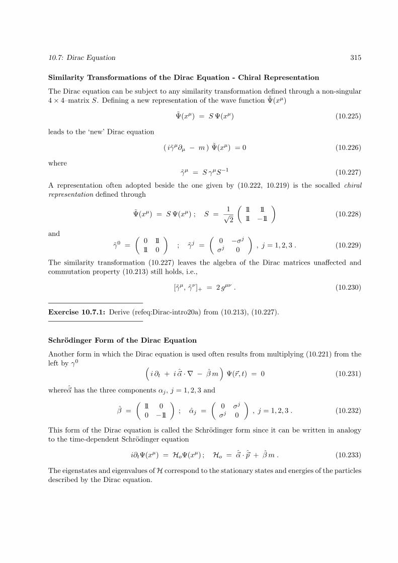
10.7: Dirac Equation 315
Similarity Transformations of the Dirac Equation - Chiral Representation
The Dirac equation can be subject to any similarity transformation defined through a non-singular4× 4–matrix S. Defining a new representation of the wave function Ψ(xµ)
Ψ(xµ) = SΨ(xµ) (10.225)
leads to the ‘new’ Dirac equation
( iγµ∂µ − m ) Ψ(xµ) = 0 (10.226)
whereγµ = S γµS−1 (10.227)
A representation often adopted beside the one given by (10.222, 10.219) is the socalled chiralrepresentation defined through
Ψ(xµ) = SΨ(xµ) ; S =1√2
(11 1111 −11
)(10.228)
and
γ0 =(
0 1111 0
); γj =
(0 −σjσj 0
), j = 1, 2, 3 . (10.229)
The similarity transformation (10.227) leaves the algebra of the Dirac matrices unaffected andcommutation property (10.213) still holds, i.e.,
[γµ, γν ]+ = 2 gµν . (10.230)
Exercise 10.7.1: Derive (refeq:Dirac-intro20a) from (10.213), (10.227).
Schrodinger Form of the Dirac Equation
Another form in which the Dirac equation is used often results from multiplying (10.221) from theleft by γ0 (
i ∂t + i ~α · ∇ − β m)
Ψ(~r, t) = 0 (10.231)
where~α has the three components αj , j = 1, 2, 3 and
β =(
11 00 −11
); αj =
(0 σj
σj 0
), j = 1, 2, 3 . (10.232)
This form of the Dirac equation is called the Schrodinger form since it can be written in analogyto the time-dependent Schrodinger equation
i∂tΨ(xµ) = HoΨ(xµ) ; Ho = ~α · ~p + β m . (10.233)
The eigenstates and eigenvalues ofH correspond to the stationary states and energies of the particlesdescribed by the Dirac equation.
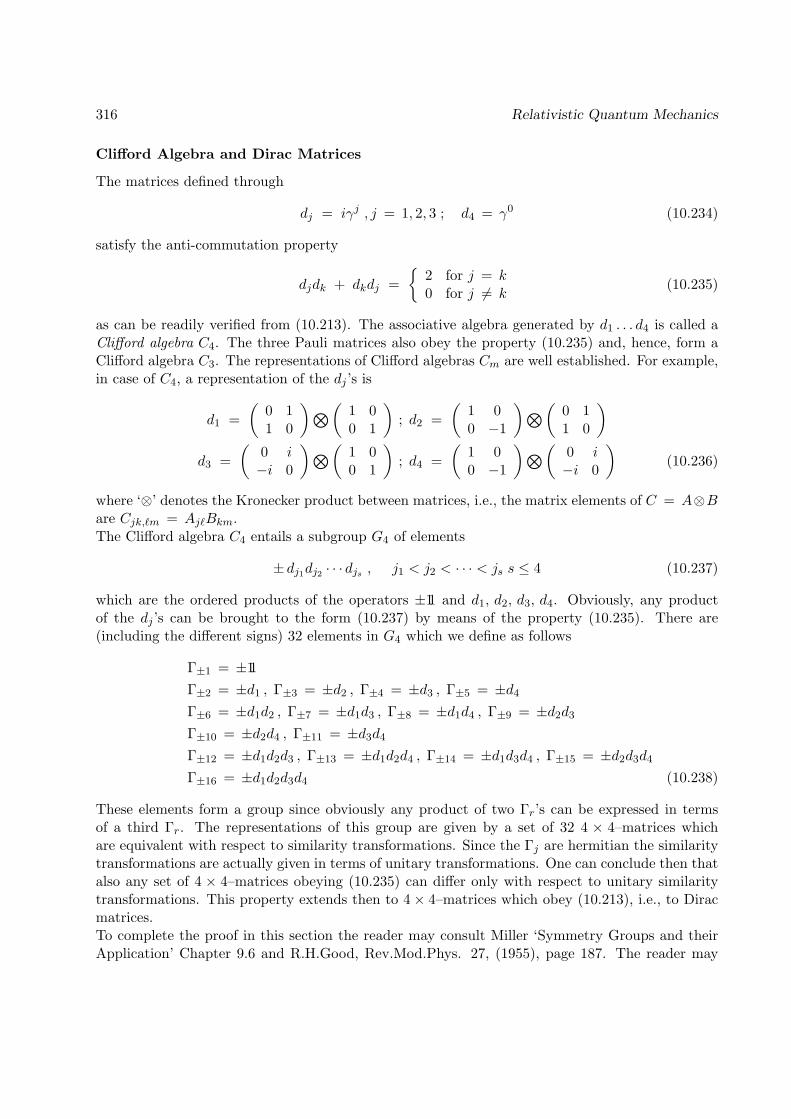
316 Relativistic Quantum Mechanics
Clifford Algebra and Dirac Matrices
The matrices defined through
dj = iγj , j = 1, 2, 3 ; d4 = γ0 (10.234)
satisfy the anti-commutation property
djdk + dkdj =
2 for j = k0 for j 6= k
(10.235)
as can be readily verified from (10.213). The associative algebra generated by d1 . . . d4 is called aClifford algebra C4. The three Pauli matrices also obey the property (10.235) and, hence, form aClifford algebra C3. The representations of Clifford algebras Cm are well established. For example,in case of C4, a representation of the dj ’s is
d1 =(
0 11 0
)⊗(1 00 1
); d2 =
(1 00 −1
)⊗(0 11 0
)d3 =
(0 i−i 0
)⊗(1 00 1
); d4 =
(1 00 −1
)⊗(0 i−i 0
)(10.236)
where ‘⊗’ denotes the Kronecker product between matrices, i.e., the matrix elements of C = A⊗Bare Cjk,`m = Aj`Bkm.The Clifford algebra C4 entails a subgroup G4 of elements
± dj1dj2 · · · djs , j1 < j2 < · · · < js s ≤ 4 (10.237)
which are the ordered products of the operators ±11 and d1, d2, d3, d4. Obviously, any productof the dj ’s can be brought to the form (10.237) by means of the property (10.235). There are(including the different signs) 32 elements in G4 which we define as follows
Γ±1 = ±11Γ±2 = ±d1 , Γ±3 = ±d2 , Γ±4 = ±d3 , Γ±5 = ±d4
Γ±6 = ±d1d2 , Γ±7 = ±d1d3 , Γ±8 = ±d1d4 , Γ±9 = ±d2d3
Γ±10 = ±d2d4 , Γ±11 = ±d3d4
Γ±12 = ±d1d2d3 , Γ±13 = ±d1d2d4 , Γ±14 = ±d1d3d4 , Γ±15 = ±d2d3d4
Γ±16 = ±d1d2d3d4 (10.238)
These elements form a group since obviously any product of two Γr’s can be expressed in termsof a third Γr. The representations of this group are given by a set of 32 4 × 4–matrices whichare equivalent with respect to similarity transformations. Since the Γj are hermitian the similaritytransformations are actually given in terms of unitary transformations. One can conclude then thatalso any set of 4 × 4–matrices obeying (10.235) can differ only with respect to unitary similaritytransformations. This property extends then to 4× 4–matrices which obey (10.213), i.e., to Diracmatrices.To complete the proof in this section the reader may consult Miller ‘Symmetry Groups and theirApplication’ Chapter 9.6 and R.H.Good, Rev.Mod.Phys. 27, (1955), page 187. The reader may
10.8: Lorentz Invariance of the Dirac Equation 317
also want to establish the unitary transformation which connects the Dirac matrices in the form(10.236) with the Dirac representation (10.219).
Exercise 7.2:Demonstrate the anti-commutation relationships (10.218) of the Pauli matrices σj .Exercise 7.3:Demonstrate the anti-commutation relationships (10.218) of the Dirac matrices γµ.Exercise 7.4:Show that from (10.214) follows that γ0 has real eigenvalues ±1 and can be represented by ahermitian matrix, and γj , j = 1, 2, 3 has imaginary eigenvalues ±i and can be represented by ananti-hermitian matrix.
10.8 Lorentz Invariance of the Dirac Equation
We want to show now that the Dirac equation is invariant under Lorentz transformations, i.e., theform of the Dirac equation is identical in equivalent frames of reference, i.e., in frames connected byLorentz transformations. The latter transformations imply that coordinates transform accordingto (10.6), i.e., x′ = Lµνx
ν , and derivatives according to (10.80). Multiplication and summationof (10.80) by Lµρ and using (10.76) yields ∂ρ = Lνρ∂
′ν , a result one could have also obtained by
applying the chain rule to (10.6). We can, therefore, transform coordinates and derivatives of theDirac equation. However, we do not know yet how to transform the 4-dimensional wave functionΨ and the Dirac matrices γµ.
Lorentz Transformation of the Bispinor State
Actually, we will approach the proof of the Lorentz invariance of the Dirac equation by testingif there exists a transformation of the bispinor wave function Ψ and of the Dirac matrices γµ
which together with the transformations of coordinates and derivatives leaves the form of the Diracequation invariant, i.e., in a moving frame should hold(
iγ′µ∂′µ − m
)Ψ′(x′µ) = 0 . (10.239)
Form invariance implies that the matrices γ′µ should have the same properties as γµ, namely,(10.213, 10.215). Except for a similarity transformation, these properties determine the matricesγ′µ uniquely, i.e., it must hold γ′µ = γµ. Hence, in a moving frame holds(
iγµ∂′µ − m)
Ψ′(x′µ) = 0 . (10.240)
Infinitesimal Bispinor State Transformation
We want to show now that a suitable transformation of Ψ(xµ) does, in fact, exist. The transfor-mation is assumed to be linear and of the form
Ψ′(x′µ) = S(Lµν) Ψ(xµ) ; x′µ = Lµνxν (10.241)

318 Relativistic Quantum Mechanics
where S(Lµν) is a non-singular 4 × 4–matrix, the coefficients of which depend on the matrix Lµνdefining the Lorentz transformation in such a way that S(Lµν) = 11 for Lµν = δµν holds. Ob-viously, the transformation (10.241) implies a similarity transformation SγµS−1. One can, hence,state that the Dirac equation (10.221) upon Lorentz transformation yields(
iS(Lηξ)γµS−1(Lηξ)Lνµ ∂′ν − m)
Ψ′(x′µ) = 0 . (10.242)
The form invariance of the Dirac equation under this transformation implies then the condition
S(Lηξ)γµS−1(Lηξ)Lνµ = γν . (10.243)
We want to determine now the 4× 4–matrix S(Lηξ) which satisfies this condition.The proper starting point for a constructiuon of S(Lηξ) is actually (10.243) in a form in which theLorentz transformation in the form Lµν is on the r.h.s. of the equation. For this purpose we exploit(10.12) in the form LνµgνσL
σρ = gµρ = gρµ. Multiplication of (10.243) from the left by Lσρgσν
yieldsS(Lηξ)γµS−1(Lηξ) gρµ = Lσρgσνγσ . (10.244)
from which, using gρµγµ = γρ, follows
S(Lηξ)γρS−1(Lηξ) = Lσργσ . (10.245)
One can finally conclude multiplying both sides by gρµ
S(Lηξ)γµS−1(Lηξ) = Lνµγν . (10.246)
The construction of S(Lηξ) will proceed using the avenue of infinitesimal transformations. We hadintroduced in (10.38) the infinitesimal Lorentz transformations in the form Lµν = δµν + εµν wherethe infinitesimal operator εµν obeyed εT = −gεg. Multiplication of this property by g from theright yields (εg)T = − εg, i.e., εg is an anti-symmetric matrix. The elements of εg are, however,εµρg
ρν = εµν and, hence, in the expression of the infinitesimal transformation
Lµν = gµν + εµν (10.247)
the infinitesimal matrix εµν is anti-symmetric.The infinitesimal transformation S(Lρσ) which corresponds to (10.247) can be expanded
S(εµν) = 11− i
4σµνε
µν (10.248)
Here σµν denote 4 × 4–matrices operating in the 4-dimensional space of the wave functions Ψ.S(εµν) should not change its value if one replaces in its argument εµν by −ενµ. It holds then
S(εµν) = 11− i
4σµνε
µν = S(−ενµ) = 11 +i
4σµνε
νµ (10.249)
from which we can conclude σµνεµν = −σµνενµ = −σνµεµν , i.e., it must hold
σµν = −σνµ . (10.250)
10.8: Lorentz Invariance of the Dirac Equation 319
One can readily show expanding SS−1 = 11 to first order in εµν that for the inverse infinitesimaltransformation holds
S−1(εµν) = 11 +i
4σµνε
µν (10.251)
Inserting (10.248, 10.251) into (10.246) results then in a condition for the generators σµν
− i4
(σαβγµ − γµσαβ ) εαβ = ενµγν . (10.252)
Since six of the coefficients εαβ can be chosen independently, this condition can actually be expressedthrough six independent conditions. For this purpose one needs to express formally the r.h.s. of(10.252) also as a sum over both indices of εαβ . Furthermore, the expression on the r.h.s., like theexpression on the l.h.s., must be symmetric with respect to interchange of the indices α and β. Forthis purpose we express
ενµγν =12εαµγα +
12εβµγβ =
12εαβ δµβγα +
12εαβ δµαγβ
=12εαβ ( δµβγα − δµαγβ ) . (10.253)
Comparing this with the l.h.s. of (10.252) results in the condition for each α, β
[σαβ , γµ ]− = 2i ( δµβγα − δµαγβ ) . (10.254)
The proper σαβ must be anti-symmetric in the indices α, β and operate in the same space as theDirac matrices. In fact, a solution of condition (10.254) is
σαβ =i
2[ γα, γβ ]− (10.255)
which can be demonstrated using the properties (10.213, 10.216) of the Dirac matrices.
Exercise 7.5:Show that the σαβ defined through (10.255) satisfy condition (10.254).
Algebra of Generators of Bispinor Transformation
We want to construct the bispinor Lorentz transformation by exponentiating the generators σµν .For this purpose we need to verify that the algebra of the generators involving addition and mul-tiplication is closed. For this purpose we inspect the properties of the generators in a particularrepresentation, namely, the chiral representation introduced above in Eqs. (10.228, 10.229). In thisrepresentation the Dirac matrices γµ = (γ0,−~γ) are
γ0 =(
0 1111 0
); γj =
(0 σj
−σj 0
), j = 1, 2, 3 . (10.256)
One can readily verify that the non-vanishing generators σµν are given by (note σµν = −σνµ, i.e.only six generators need to be determined)
σ0j =i
2[γ0, γj ] =
(−iσj 0
0 iσj
); σjk = [γj , γk] = εjk`
(σ` 00 σ`
). (10.257)
320 Relativistic Quantum Mechanics
Obviously, the algebra of these generators is closed under addition and multiplication, since bothoperations convert block-diagonal operators(
A 00 B
)(10.258)
again into block-diagonal operators, and since the algebra of the Pauli matrices is closed.We can finally note that the closedness of the algebra of the generators σµν is not affected bysimilarity transformations and that, therefore, any representation of the generators, in particular,the representation (10.255) yields a closed algebra.
Finite Bispinor Transformation
The closedness of the algebra of the generators σµν defined through (10.248) allows us to write thetransformation S for any, i.e., not necessarily infinitesimal, εµν in the exponential form
S = exp(− i
4σµνε
µν
). (10.259)
We had stated before that the transformation S is actually determined through the Lorentz trans-formation Lµν . One should, therefore, be able to state S in terms of the same parameters ~w and~ϑ as the Lorentz transformation in (10.51). In fact, one can express the tensor εµν through ~w and~ϑ using εµν = εµρg
ρν and the expression (10.44)
εµν =
0 −w1 −w2 −w3
w1 0 ϑ3 −ϑ2
w2 −ϑ3 0 ϑ1
w3 ϑ2 −ϑ1 0
(10.260)
Inserting this into (10.259) yields the desired connection between the Lorentz transformation (10.51)and S.In order to construct an explicit expression of S in terms of ~w and ~ϑ we employ again the chiralrepresentation. In this representation holds
− i4 σµνε
µν = − i2
(σ01ε01 + σ02ε
02 + σ03ε03 + σ12ε
12 + σ13ε13 + σ23ε
23)
=12
((~w − i~ϑ) · ~σ 0
0 −(~w + i~ϑ) · ~σ
). (10.261)
We note that this operator is block-diagonal. Since such operator does not change its block-diagonalform upon exponentiation the bispinor transformation (10.259) becomes in the chiral representation
S(~w, ~ϑ) =
(e
12
(~w− i~ϑ)·~σ 00 e−
12
(~w+ i~ϑ)·~σ
)(10.262)
This expression allows one to transform according to (10.241) bispinor wave functions from oneframe of reference into another frame of reference.
10.8: Lorentz Invariance of the Dirac Equation 321
Current 4-Vector Associated with Dirac Equation
We like to derive now an expression for the current 4-vector jµ associated with the Dirac equationwhich satisfies the conservation law
∂µjµ = 0 . (10.263)
Starting point are the Dirac equation in the form (10.221) and the adjoint Dirac equation (10.224).Multiplying (10.221) from the left by Ψ†(xµ)γ0, (10.224) from the right by Ψ(xµ), and additionyields
Ψ†(xµ)γ0
(iγµ∂µ + iγµ
←∂µ
)Ψ(xµ) = 0 . (10.264)
The last result can be written∂µ Ψ†(xν)γ0γµΨ(xν) = 0 , (10.265)
i.e., the conservation law (10.263) does hold, in fact, for
jµ(xµ) = (ρ, ~j) = Ψ†(xµ)γ0γµΨ(xµ) . (10.266)
The time-like component ρ of jµ
ρ(xµ) = Ψ†(xµ)Ψ(xµ) =4∑s=1
|ψs(xµ)|2 (10.267)
has the desired property of being positive definite.The conservation law (10.263) allows one to conclude that jµ must transform like a contravariant4-vector as the notation implies. The reason is that the r.h.s. of (10.263) obviously is a scalarunder Lorentz transformations and that the left hand side must then also transform like a scalar.Since ∂µ transforms like a covariant 4-vector, jµ must transform like a contravariant 4-vector. Thistransformation behaviour can also be deduced from the transformation properties of the bispinorwave function Ψ(xµ). For this purpose we prove first the relationship
S−1 = γ0 S†γ0 . (10.268)
We will prove this property in the chiral representation. Obviously, the property applies then inany representation of S.For our proof we note first
S−1(~w, ~ϑ) = S(−~w,−~ϑ) =
(e−
12
(~w− i~ϑ)·~σ 00 e
12
(~w+ i~ϑ)·~σ
)(10.269)
One can readily show that the same operator is obtained evaluating
γ0S†(~w, ~ϑ)γ0 =(
0 1111 0
) (e
12
(~w+ i~ϑ)·~σ 00 e−
12
(~w− i~ϑ)·~σ
) (0 1111 0
). (10.270)
We conclude that (10.268) holds for the bispinor Lorentz transformation.We will now determine the relationship between the flux
j′µ = Ψ′†(x′µ)γ0γµΨ′(x′) (10.271)

322 Relativistic Quantum Mechanics
in a moving frame of reference and the flux jµ in a frame at rest. Note that we have assumedin (10.271) that the Dirac matrices are independent of the frame of reference. One obtains using(10.268)
j′µ = Ψ†(xµ)S†γ0γµSΨ(xµ) = Ψ†(xµ)γ0S−1γµSΨ(xµ) . (10.272)
With S−1(Lηξ) = S((L−1)ηξ) one can restate (10.246)
S−1(Lηξ)γµS(Lηξ) = (L−1)νµγν = (L−1)νµγν = Lµνγν . (10.273)
where we have employed (10.76). Combining this with (10.272) results in the expected transfor-mation behaviour
j′µ = Lµνj
ν . (10.274)
10.9 Solutions of the Free Particle Dirac Equation
We want to determine now the wave functions of free particles described by the Dirac equation.Like in non-relativistic quantum mechanics the free particle wave function plays a central role, notonly as the most simple demonstration of the theory, but also as providing a basis in which the wavefunctions of interacting particle systems can be expanded and characterized. The solutions providealso a complete, orthonormal basis and allows one to quantize the Dirac field Ψ(xµ) much like theclassical electromagnetic field is quantized through creation and annihilation operators representingfree electromagnetic waves of fixed momentum and frequency.In case of non-relativistic quantum mechanics the free particle wave function has a single componentψ(~r, t) and is determined through the momentum ~p ∈ R
3. In relativistic quantum mechanics aDirac particle can also be characterized through a momentum, however, the wave function has fourcomponents which invite further characterization of the free particle state. In the following wewant to provide this characterization, specific for the Dirac free particle.We will start from the Dirac equation in the Schrodinger form (10.231, 10.232, 10.233)
i∂tΨ(xµ) = HoΨ(xµ) . (10.275)
The free particle wave function is an eigenfunction of Ho, a property which leads to the energy–momentum (dispersion) relationship of the Dirac particle. The additional degrees of freedom de-scribed by the four components of the bispinor wave function require, as just mentioned, additionalcharacterizations, i.e., the identification of observables and their quantum mechanical operators, ofwhich the wave functions are eigenfunctions as well. As it turns out, only two degrees of freedomof the bispinor four degrees of freedom are independent [c.f. (10.282, 10.283)]. The independentdegrees of freedom allow one to choose the states of the free Dirac particle as eigenstates of the4-momentum operator pµ and of the helicity operator Γ ∼ ~σ · ~p/|~p| introduced below. These opera-tors, as is required for the mentioned property, commute with each other. The operators commutealso with Ho in (10.233).Like for the free particle wave functions of the non-relativistic Schrodinger and the Klein–Gordonequations one expects that the space–time dependence is governed by a factor exp[i(~p · ~r − εt)].As pointed out, the Dirac particles are described by 4-dimensional, bispinor wave functions and weneed to determine corresponding components of the wave function. For this purpose we consider

10.9: Solutions of the Free Particle Dirac Equation 323
the following form of the free Dirac particle wave function
Ψ(xµ) =(φ(xµ)χ(xµ)
)=(φoχo
)ei(~p·~r− εt) (10.276)
where ~p and ε together represent four real constants, later to be identified with momentum andenergy, and φo, χo each represent a constant, two-dimensional spinor state. Inserting (10.276) into(10.231, 10.232) leads to the 4-dimensional eigenvalue problem(
m ~σ · ~p~σ · ~p −m
) (φoχo
)= ε
(φoχo
). (10.277)
To solve this problem we write (10.277) explicitly
(ε − m) 11φo − ~σ · ~pχo = 0−~σ · ~p φo + (ε + m) 11χo = 0 . (10.278)
Multiplication of the 1st equation by (ε +m)11 and of the second equation by −~σ ·~p and subtractionof the results yields the 2-dimensional equation[
(ε2 − m2) 11 − (~σ · ~p)2]φo = 0 . (10.279)
According to the property (5.234) of Pauli matrices holds (~σ ·~p)2 = ~p 211. One can, hence, concludefrom (10.279) the well-known relativistic dispersion relationship
ε2 = m2 + ~p 2 (10.280)
which has a positive and a negative solution
ε = ±E(~p) , E(~p) =√m2 + ~p 2 . (10.281)
Obviously, the Dirac equation, like the Klein–Gordon equation, reproduce the classical relativisticenergy–momentum relationships (10.93, 10.94)Equation (10.278) provides us with information about the components of the bispinor wave function(10.276), namely φo and χo are related as follows
φ0 =~σ · ~pε−m
χ0 (10.282)
χo =~σ · ~pε + m
φ0 , (10.283)
where ε is defined in (10.281). These two relationships are consistent with each other. In fact, onefinds using (5.234) and (10.280)
~σ · ~pε+m
φ0 =(~σ · ~p)2
(ε+m) (ε+m)χ0 =
~p 2
ε2 −m2χ0 = χ0 . (10.284)
The relationships (10.282, 10.283) imply that the bispinor part of the wave function allows onlytwo degrees of freedom to be chosen independently. We want to show now that these degrees offreedom correspond to a spin-like property, the socalled helicity of the particle.

324 Relativistic Quantum Mechanics
For our further characterization we will deal with the positive and negative energy solutions [cf.(10.281)] separately. For the positive energy solution, i.e., the solution for ε = +E(~p), we presentφo through the normalized vector
φo =(u1
u2
)= u ∈ C2 , u†u = |u1|2 + |u2|2 = 1 . (10.285)
The corresponding free Dirac particle is then described through the wave function
Ψ(~p,+|xµ) = N+(~p)
(u
~σ·~pE(~p) +m u
)ei(~p·~r− εt) , ε = +E(~p) . (10.286)
Here N+(~p) is a constant which will be chosen to satisfy the normalization condition
Ψ†(~p,+) γ0 Ψ†(~p,+) = 1 , (10.287)
the form of which will be justified further below. Similarly, we present the negative energy solution,i.e., the solution for ε = −E(~p), through χo given by
χo =(u1
u2
)= u ∈ C2 , u†u = |u1|2 + |u2|2 = 1 . (10.288)
corresponding to the wave function
Ψ(~p,−|xµ) = N−(~p)
(−~σ·~p
E(~p) +m uu
)ei(~p·~r− εt) , ε = −E(~p) . (10.289)
Here N−(~p) is a constant which will be chosen to satisfy the normalization condition
Ψ†(~p,+) γ0 Ψ†(~p,+) = −1 , (10.290)
which differs from the normalization condition (10.287) in the minus sign on the r.h.s. The formof this condition and of (10.287) will be justified now.First, we demonstrate that the product Ψ†(~p,±)γ0Ψ(~p,±), i.e., the l.h.s. of (10.287, 10.290), isinvariant under Lorentz transformations. One can see this as follows: Let Ψ(~p,±) denote thesolution of a free particle moving with momentum ~p in the laboratory frame, and let Ψ(0,±)denote the corresponding solution of a particle in its rest frame. The connection between thesolutions, according to (10.241), is Ψ(~p,±) = SΨ(0,±) , where S is given by (10.259). Hence,
Ψ†(~p,±) γ0 Ψ(~p,±) =(
Ψ†(0,±)S†)γ0 SΨ(0,±)
= Ψ†(0,±)(γ0 S−1 γ0
)γ0 SΨ(0,±)
= Ψ†(0,±) γ0 Ψ(0,±). (10.291)
Note that we have used that, according to (10.268), S−1 = γ0S†γ0 and, hence, S† = γ0S−1γ0.We want to demonstrate now that the signs on the r.h.s. of (10.287, 10.290) should differ. For thispurpose we consider first the positive energy solution. Employing (10.286) for ~p = 0 yields, usingγ0 as given in (10.219) and u†u = 1 [c.f. (10.285)],
Ψ†(0,+) γ0 Ψ(0,+) = |N+(0)|2 (u†, 0) γ0
(u0
)= |N+(0)|2 . (10.292)

10.9: Solutions of the Free Particle Dirac Equation 325
The same calculation for the negative energy wave function as given in (10.289) yields
Ψ†(0,−) γ0 Ψ(0,−) = |N−(0)|2 (0, u†) γ0
(0u
)= − |N−(0)|2 . (10.293)
Obviously, this requires the choice of a negative side on the r.h.s. of (10.290) to assign a positivevalue to |N−(0)|2. We can also conclude from our derivation
N±(0) = 1 . (10.294)
We want to determine now N±(~p) for arbitrary ~p. We consider first the positive energy solution.Condition (10.287) written explicitly using (10.286) is
N 2+(~p)
((u∗)T ,
[~σ · ~p
E(~p) + mu∗]T)
γo
(u
~σ·~pE(~p) +m u
)= 1 (10.295)
Evaluating the l.h.s. using γ0 as given in (10.219) yields
N 2+(~p)
[u†u − u†
(~σ · ~p)2
(E(~p) + m)2u]
= 1 . (10.296)
Replacing (~σ · ~p)2 by ~p 2 [c.f. (5.234)] and using the normalization of u in (10.285) results in
N 2+(~p)
[1 − ~p 2
(E(~p) + m)2
]= 1 (10.297)
from which follows
N+(~p) =
√(m + E(~p) )2
(m + E(~p) )2 − ~p 2. (10.298)
Noting
(m + E(~p) )2 − ~p 2 = m2 − ~p 2 + 2mE(~p) + E2(~p) = 2(m + E(~p))m (10.299)
the normalization coefficient (10.298) becomes
N+(~p) =
√m + E(~p)
2m. (10.300)
This result completes the expression for the wave function (10.286).
Exercise 7.6: Show that the normalization condition
N ′2+ (~p)
((u∗)T ,
[~σ · ~p
E(~p) + mu∗]T) ( u
~σ·~pE(~p) +m u
)= 1 (10.301)
yields the normalization coefficient
N ′+(~p) =
√m + E(~p)
2 E(~p). (10.302)

326 Relativistic Quantum Mechanics
We consider now the negative energy solution. Condition (10.290) written explicitly using (10.289)is
N 2−(~p)
([−~σ · ~p
E(~p) + mu∗]T, (u∗)T
)γo
(−~σ·~p
E(~p) +m uu
)= −1 (10.303)
Evaluating the l.h.s. yields
N 2−(~p)
[u†
(~σ · ~p)2
(E(~p) + m)2u − u†u
]= −1 . (10.304)
This condition is, however, identical to the condition (10.296) for the normalization constant N+(~p)of the positive energy solution. We can, hence, conclude
N−(~p) =
√m + E(~p)
2m(10.305)
and, thereby, have completed the determination for the wave function (10.289).The wave functions (10.286, 10.289, 10.300) have been constructed to satisfy the free particle Diracequation (10.275). Inserting (10.286) into (10.275) yields
Ho Ψ(~p, λ|xµ) = λE(~p) Ψ(~p, λ|xµ) , (10.306)
i.e., the wave functions constructed represent eigenstates of Ho. The wave functions are alsoeigenstates of the momentum operator i∂µ, i.e.,
i∂µΨ(~p, λ|xµ) = pµ Ψ(~p, λ|xµ) (10.307)
where pµ = (ε,−~p). This can be verified expressing the space–time factor of Ψ(~p, λ|xµ) in 4-vectornotation, i.e., exp[i(~p · ~r − εt)] = exp(ipµxµ).
Helicity
The free Dirac particle wave functions (10.286, 10.289) are not completely specified, the two com-ponents of u indicate another degree of freedom which needs to be defined. This degree of freedomdescribes a spin–1
2 attribute. This attribute is the so-called helicity, defined as the component ofthe particle spin along the direction of motion. The corresponding operator which measures thisobservable is
Λ =12σ ·
~p
|~p|. (10.308)
Note that ~p represents here an operator, not a constant vector. Rather than considering theobservable (10.307) we investigate first the observable due to the simpler operator ~σ · ~p. Wewant to show that this operator commutes with Ho and ~p to ascertain that the free particle wavefunction can be simultaneously an eigenvector of all three operators. The commutation property[~σ · ~p, pj ] = 0 , j = 1, 2, 3 is fairly obvious. The property [~σ · ~p,Ho] = 0 follows from (10.233) andfrom the two identities(
11 00 −11
)(~σ 00 ~σ
)· ~p −
(~σ 00 ~σ
)· ~p(
11 00 −11
)= 0 (10.309)
10.9: Solutions of the Free Particle Dirac Equation 327
and (0 ~σ~σ 0
)· ~p(~σ 00 ~σ
)· ~p −
(~σ 00 ~σ
)· ~p(
0 ~σ~σ 0
)· ~p
=
(0 (~σ · ~p)2
(~σ · ~p)2 0
)−
(0 (~σ · ~p)2
(~σ · ~p)2 0
)= 0 . (10.310)
We have shown altogether that the operators ~p,Ho and ~σ·~p commute with each other and, hence, canbe simultaneously diagonal. States which are simultaneously eigenvectors of these three operatorsare also simulteneously eigenvectors of the three operators ~p, Ho and Λ defined in (10.308) above.The condition that the wave functions (10.286) are eigenfunctions of Λ as well will specify now thevectors u.Since helicity is defined relative to the direction of motion of a particle the characterization of uas an eigenvector of the helicity operator, in principle, is independent of the direction of motionof the particle. We consider first the simplest case that particles move along the x3–direction, i.e.,~p = (0, 0, p3). In this case Λ = 1
2σ3.
We assume first particles with positive energy, i.e., ε = +E(~p). According to the definition (5.224)of σ3 the two u vectors (1, 0)T and (0, 1)T are eigenstates of 1
2σ3 with eigenvalues ±1
2 . Therefore,the wave functions which are eigenstates of the helicity operator, are
Ψ(pe3,+,+12 |~r, t) = Np
(
10
)p
m+Ep
(10
) ei(px
3−Ept)
Ψ(pe3,+,−12 |~r, t) = Np
(
01
)−p
m+Ep
(01
) ei(px
3−Ept) (10.311)
where e3 denotes the unit vector in the x3-direction and where
Ep =√m2 + p2 ; Np =
√m + Ep
2m. (10.312)
We assume now particles with negative energy, i.e., ε = −E(~p). The wave functions which areeigenfunctions of the helicity operator are in this case
Ψ(pe3,−,+12 |~r, t) = Np
−p
m+Ep
(10
)(
10
) ei(px
3 +Ept)
Ψ(pe3,−,−12 |~r, t) = Np
p
m+Ep
(01
)(
01
) ei(px
3 +Ept) (10.313)
where Ep and Np are defined in (10.312).
328 Relativistic Quantum Mechanics
To obtain free particle wave functions for arbitrary directions of ~p one can employ the wave functions(10.311, 10.313) except that the states (1, 0)T and (0, 1)T have to be replaced by eigenstates u±(~p)of the spin operator along the direction of ~p. These eigenstates are obtained through a rotationaltransformation (5.222, 5.223) as follows
u(~p,+12
) = exp(− i
2~ϑ(~p) · ~σ
) (10
), (10.314)
u(~p,−12
) = exp(− i
2~ϑ(~p) · ~σ
) (01
)(10.315)
where~ϑ(~p) =
e3 × ~p|~p|
∠(e3, ~p) (10.316)
describes a rotation which aligns the x3–axis with the direction of ~p. [One can also express therotation through Euler angles α, β, γ , in which case the transformation is given by (5.220).] Thecorresponding free particle wave functions are then
Ψ(~p,+,+12 |~r, t) = Np
(u(~p,+1
2)p
m+Epu(~p,+1
2)
)ei(~p·~r−Ept) (10.317)
Ψ(~p,+,−12 |~r, t) = Np
(u(~p,−1
2)−p
m+Epu(~p,−1
2)
)ei(~p·~r−Ept) (10.318)
Ψ(~p,−,+12 |~r, t) = N√
( −pm+Ep
u(~p,+12)
u(~p,+12)
)ei(~p·~r+Ept) (10.319)
Ψ(~p,−,−12 |~r, t) = Np
(p
m+Epu(~p,−1
2)
u(~p,−12)
)ei(~p·~r+Ept) (10.320)
where Ep and N are again given by (10.312).
Generating Solutions Through Lorentz Transformation
The solutions (10.311, 10.312) can be obtained also by means of the Lorentz transformation (10.262)for the bispinor wave function and the transformation (10.123). For this purpose one starts fromthe solutions of the Dirac equation in the chiral representation (10.226, 10.229), denoted by , foran ~r–independent wave function, i.e., a wave function which represents free particles at rest. Thecorresponding wave functions are determined through(
iγ0∂t − m)
Ψ(t) = 0 . (10.321)
and are
Ψ(p = 0, +, 12 |t) = 1√
2
1010
e−imt ,

10.9: Solutions of the Free Particle Dirac Equation 329
Ψ(p = 0, +, −12 |t) = 1√
2
0101
e−imt ,
Ψ(p = 0, −, 12 |t) = 1√
2
10−10
e+imt ,
Ψ(p = 0, −, −12 |t) = 1√
2
010−1
e+imt . (10.322)
The reader can readily verify that transformation of these solutions to the Dirac representationsasdefined in (10.228) yields the corresponding solutions (10.311, 10.313) in the p → 0 limit. Thiscorrespondence justifies the characterization ±,±1
2 of the wave functions stated in (10.322).The solutions (10.322) can be written in spinor form
1√2
(φoχo
)e∓imt , φo , χo ∈
(10
),
(01
)(10.323)
Transformation (10.262) for a boost in the x3–direction, i.e., for ~w = (0, 0, w3), yields for theexponential space–time dependence according to (10.174, 10.176)
∓imt → i ( p3x3 ∓ Et ) (10.324)
and for the bispinor part according to (10.262)(φoχo
)→
(e
12w3σ3
00 e−
12w3σ3
) (φoχo
)=
(e
12w3σ3
φo
e−12w3σ3
χo
). (10.325)
One should note that φo, χo are eigenstates of σ3 with eigenvalues ±1. Applying (10.324, 10.325)to (10.323) should yield the solutions for non-vanishing momentum p in the x3–direction. For theresulting wave functions in the chiral representation one can use then a notation corresponding tothat adopted in (10.311)
Ψ(p(w3)e3, +, +12 |~r, t) =
1√2
e12w3
(10
)e−
12w3
(10
) ei(px
3−Ept)
Ψ(p(w3)e3, +, −12 |~r, t) =
1√2
e−12w3
(01
)e
12w3
(01
) ei(px
3−Ept)
330 Relativistic Quantum Mechanics
Ψ(p(w3)e3, −, +12 |~r, t) =
1√2
e12w3
(10
)−e−
12w3
(10
) ei(px
3 +Ept)
Ψ(p(w3)e3, −, −12 |~r, t) =
1√2
e−12w3
(01
)− e
12w3
(01
) ei(px
3 +Ept) (10.326)
where according to (10.61) p(w3) = m sinhw3. Transformation to the Dirac representation bymeans of (10.228) yields
Ψ(p(w3)e3, +, +12 |~r, t) =
coshw32
(10
)sinhw3
2
(10
) ei(px
3−Ept)
Ψ(p(w3)e3, +, −12 |~r, t) =
coshw32
(01
)− sinhw3
2
(01
) ei(px
3−Ept)
Ψ(p(w3)e3, −, +12 |~r, t) =
sinhw32
(10
)coshw3
2
(10
) ei(px
3 +Ept)
Ψ(p(w3)e3, −, −12 |~r, t) =
− sinhw32
(01
)coshw3
2
(01
) ei(px
3 +Ept) (10.327)
Employing the hyperbolic function properties
coshx
2=
√coshx + 1
2, sinh
x
2=
√coshx − 1
2, (10.328)
the relationship (10.61) between the parameter w3 and boost velocity v3, and the expression (10.311)for Ep one obtains
coshw32 =
1√2
√√√√√ 11 − v2
3
+ 1 =1√2
√√√√√1 +v2
3
1 − v23
+ 1
=
√√√√√√m2 + m2v2
3
1− v23
+ m
2m=
√Ep + m
2m(10.329)

10.9: Invariance of Dirac Equation Revisited 331
and similarly
sinhw3
2=
√Ep − m
2m=
p√2m (Ep + m)
(10.330)
Inserting expressions (10.329, 10.330) into (10.327), indeed, reproduces the positive energy wavefunctions (10.311) as well as the negative energy solutions (10.313) for −p. The change of sign forthe latter solutions had to be expected as it was already noted for the negative energy solutions ofthe Klein–Gordon equation (10.168–10.176).
Invariance of Dirac Equation Revisited
At this point we like to provide a variation of the derivation of (10.243), the essential propertystating the Lorentz–invariance of the Dirac equation. Actually, we will derive this equation onlyfor infinitesimal transformations, which however, is sufficient since (1) it must hold then for anyfinite transformation, and since (2) the calculations following (10.243) considered solely the limitof infinitesimal transformations anyway.The reason why we provide another derivation of (10.243) is to familiarize ourselves with a formu-lation of Lorentz transformations of the bispinor wave finction Ψ(xµ) which treats the spinor andthe space-time part of the wave function on the same footing. Such description will be essential forthe formal description of Lorentz invariant wave equations for arbitray spin further below.In the new derivation we consider the particle described by the wave function transformed, but notthe observer. This transformation, refered to as the active transformation, expresses the system inthe old coordinates. The transformation is
Ψ′(xµ) = S(Lηξ) ρ(Lηξ) Ψ(xµ) (10.331)
where S(Lηξ) denotes again the transformation acting on the bispinor character of the wave functionΨ(xµ) and where ρ(Lηξ) denotes the transformation acting on the space-time character of thewave function Ψ(xµ). ρ(Lηξ) has been defined in (10.123) above and characterized there. Suchtransformation had been applied by us, of course, when we generated the solutions Ψ(~p, λ,Λ|xµ)from the solutions describing particles at rest Ψ(~p = 0, λ,Λ|t). We expect, in general, that if Ψ(xµ)is a solution of the Dirac equation that Ψ′(xµ) as given in (10.331) is a solution as well. Makingthis expectation a postulate allows one to derive the condition (10.243) and, thereby, the propertransformation S(Lηξ).To show this we rewrite the Dirac equation (10.221) using (10.331)(
i S(Lηξ)γµS−1(Lηξ) ρ(Lηξ)∂µρ−1(Lηξ) − m)
Ψ′(xµ) = 0 (10.332)
Here we have made use of the fact that S(Lηξ) commutes with ∂µ and ρ(Lηξ) commutes with γµ.The fact that any such Ψ′(xµ) is a solution of the Dirac equation allows us to conclude
S(Lηξ)γµS−1(Lηξ) ρ(Lηξ)∂µρ−1(Lηξ) = γν∂ν (10.333)
which is satisfied in case that the following conditions are met
ρ(Lηξ)∂µρ−1(Lηξ) = Lνµ ∂ν ;S(Lηξ)γµS−1(Lηξ)Lνµ = γν . (10.334)

332 Relativistic Quantum Mechanics
We will demonstrate now that the first condition is satisfied by ρ(Lηξ). The second condition isidentical to (10.243) and, of course, it is met by S(Lηξ) as given in the chiral representation by(10.262).As mentioned already we will show condition (10.334) for infinitesimal Lorentz transformationsLηξ. We will proceed by employing the generators (10.128) to express ρ(Lηξ) in its infinitesimalform and evaluate the expression(
11 + ε~ϑ · ~J + ε~w · ~K)∂µ
(11 − ε~ϑ · ~J − ε~w · ~K
)= ∂µ + εMν
µ∂ν + O(ε2) (10.335)
The result will show that the matrix Mνµ is identical to the generators of Lνµ for the six choices ~ϑ =
(1, 0, 0), ~w = (0, 0, 0), ~ϑ = (0, 1, 0), ~w = (0, 0, 0), . . . , ϑ = (0, 0, 0), ~w = (0, 0, 1) . Inspection of(10.335) shows that we need to demonstrate
[J`, ∂µ] = (J`)νµ∂ν ; [K`, ∂µ] = (K`)νµ∂ν . (10.336)
We will proceed with this task considering all six cases:
[J1, ∂µ] = [x3∂2 − x2∂3, ∂µ] =
0 µ = 00 µ = 1∂3 µ = 2−∂2 µ = 3
(10.337)
[J2, ∂µ] = [x1∂3 − x3∂1, ∂µ] =
0 µ = 0
−∂3 µ = 10 µ = 2∂1 µ = 3
(10.338)
[J3, ∂µ] = [x2∂1 − x1∂2, ∂µ] =
0 µ = 0∂2 µ = 1−∂1 µ = 2
0 µ = 3
(10.339)
[K1, ∂µ] = [x0∂1 + x1∂0, ∂µ] =
−∂1 µ = 0−∂0 µ = 1
0 µ = 20 µ = 3
(10.340)
[K2, ∂µ] = [x0∂2 + x2∂0, ∂µ] =
−∂2 µ = 0
0 µ = 1−∂0 µ = 2
0 µ = 3
(10.341)
[K3, ∂µ] = [x0∂3 + x3∂0, ∂µ] =
−∂3 µ = 0
0 µ = 10 µ = 2
−∂0 µ = 3
(10.342)
One can readily convince oneself that these results are consistent with (10.336). We have demon-strated, therefore, that any solution Ψ(xµ) transformed according to (10.331) is again a solution ofthe Dirac equation, i.e., the Dirac equation is invariant under active Lorentz transformations.
10.10: Dirac Particles in Electromagnetic Field 333
10.10 Dirac Particles in Electromagnetic Field
We like to provide now a description for particles governed by the Dirac equation which includesthe coupling to an electromagnetic field in the minimum coupling description. Following the re-spective procedure developed for the Klein-Gordon equation in Sect. 10.6 we assume that the fieldis described through the 4-vector potential Aµ and, accordingly, we replace in the Dirac equationthe momentum operator pµ = i∂µ by i∂µ − qAµ where q is the charge of the respective particles(see Table 10.1 in Sect 10.6 above). Equivalently, we replace the operator ∂µ by ∂µ + iqAµ. TheDirac equation (10.221) reads then
[ iγµ(∂µ + iqAµ) − m ] Ψ(xν) = 0 (10.343)
One may also include the electromagnetic field in the Dirac equation given in the Schrodinger form(10.233) by replacing i∂t by (see Table 10.1) i∂t − qV and ~p by
~π = ~p − q ~A . (10.344)
The Dirac equation in the Schrodinger form reads then
i∂tΨ(xµ) =(~α · ~π + qV + β m
)Ψ(xµ) (10.345)
where ~α and β are defined in (10.232).
Non-Relativistic Limit
We want to consider now the Dirac equation (10.345) in the so-called non-relativistic limit in whichall energies are much smaller than m, e.g., for the scalar field V in (10.345) holds
|qV | << m . (10.346)
For this purpose we choose the decomposition
Ψ(xµ) =(φ(xµ)χ(xµ)
). (10.347)
Using the notation ~σ = (σ1, σ2, σ3)T one obtains then
i∂tφ = ~σ · ~π χ + qV φ + mφ (10.348)i∂tχ = ~σ · ~π φ + qV χ − mχ . (10.349)
We want to focus on the stationary positive energy solution. This solution exhibits a time-dependence exp[−i(m + ε)t] where for ε holds in the non-relativistic limit |ε| << m. Accordingly,we define
φ(xµ) = e−imt Φ(xµ) (10.350)χ(xµ) = e−imtX (xµ) (10.351)
334 Relativistic Quantum Mechanics
and assume that for the time-derivative of Φ and X holds∣∣∣∣∂tΦΦ
∣∣∣∣ << m ,
∣∣∣∣∂tXX∣∣∣∣ << m . (10.352)
Using (10.350, 10.351) in (10.348, 10.349) yields
i∂tΦ = ~σ · ~πX + qV Φ (10.353)i∂tX = ~σ · ~πΦ + qV X − 2mX . (10.354)
The properties (10.346, 10.352) allow one to approximate (10.354)
0 ≈ ~σ · ~π Φ − 2m X . (10.355)
and, accordingly, one can replace X in (10.353) by
X ≈ ~σ · ~π2m
Φ (10.356)
to obtain a closed equation for Φ
i∂tΦ ≈
(~σ · ~π
)2
2mΦ + qV Φ . (10.357)
Equation (10.356), due to the m−1 factor, identifies X as the small component of the bi-spinorwave function which, henceforth, does not need to be considered anymore.Equation (10.357) for Φ can be reformulated by expansion of (~σ · ~π)2. For this purpose we employthe identity (5.230), derived in Sect. 5.7, which in the present case states
(~σ · ~π)2 = ~π2
+ i ~σ · (~π × ~π) . (10.358)
For the components of ~π × ~π holds(~π × ~π
)`
= εjk` (πjπk − πkπj ) = εjk` [πj , π`] . (10.359)
We want to evaluate the latter commutator. One obtains
[πj , πk] = [1i∂j + qAj ,
1i∂k + qAk]
= [1i∂j ,
1i∂k]︸ ︷︷ ︸
= 0
+ q [Aj ,1i∂k] + q [
1i∂j , Ak] + q2 [Aj , Ak]︸ ︷︷ ︸
= 0
=q
i[Aj , ∂k] +
q
i[∂j , Ak] . (10.360)
For an arbitrary function f(~r) holds
( [Aj , ∂k] + [∂j , Ak] ) f = ( ∂jAk − Ak∂j + Aj∂k − ∂kAj ) f . (10.361)
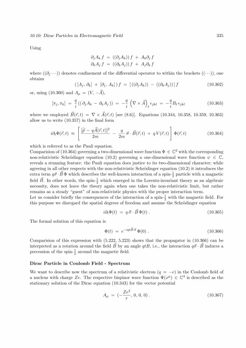
10.10: Dirac Particles in Electromagnetic Field 335
Using
∂jAk f = ((∂jAk)) f + Ak∂j f
∂kAj f = ((∂kAj)) f + Aj∂k f
where ((∂j · · ·)) denotes confinement of the differential operator to within the brackets ((· · ·)), oneobtains
( [Aj , ∂k] + [∂j , Ak] ) f = [ ((∂jAk)) − ((∂kAj)) ] f (10.362)
or, using (10.360) and Aµ = (V, − ~A),
[πj , πk] =q
i(( ∂jAk − ∂kAj )) = −q
i
(∇× ~A
)`εjk` = −q
iB` εjk` (10.363)
where we employed ~B(~r, t) = ∇ × ~A(~r, t) [see (8.6)]. Equations (10.344, 10.358, 10.359, 10.363)allow us to write (10.357) in the final form
i∂tΦ(~r, t) ≈
[[~p − q ~A(~r, t)]2
2m− q
2m~σ · ~B(~r, t) + q V (~r, t)
]Φ(~r, t) (10.364)
which is referred to as the Pauli equation.Comparision of (10.364) governing a two-dimensional wave function Φ ∈ C2 with the correspondingnon-relativistic Schrodinger equation (10.2) governing a one-dimensional wave function ψ ∈ C,reveals a stunning feature: the Pauli equation does justice to its two-dimensional character; whileagreeing in all other respects with the non-relativistic Schrodinger equation (10.2) it introduces theextra term q~σ · ~B Φ which describes the well-known interaction of a spin-1
2 particle with a magneticfield ~B. In other words, the spin-1
2 which emerged in the Lorentz-invariant theory as an algebraicnecessity, does not leave the theory again when one takes the non-relativistic limit, but ratherremains as a steady “guest” of non-relativistic physics with the proper interaction term.Let us consider briefly the consequences of the interaction of a spin-1
2 with the magnetic field. Forthis purpose we disregard the spatial degrees of freedom and assume the Schrodinger equation
i∂tΦ(t) = q ~σ · ~B Φ(t) . (10.365)
The formal solution of this equation is
Φ(t) = e−iqt~B·~σ Φ(0) . (10.366)
Comparision of this expression with (5.222, 5.223) shows that the propagator in (10.366) can beinterpreted as a rotation around the field ~B by an angle qtB, i.e., the interaction q~σ · ~B induces aprecession of the spin-1
2 around the magnetic field.
Dirac Particle in Coulomb Field - Spectrum
We want to describe now the spectrum of a relativistic electron (q = −e) in the Coulomb field ofa nucleus with charge Ze. The respective bispinor wave function Ψ(xµ) ∈ C4 is described as thestationary solution of the Dirac equation (10.343) for the vector potential
Aµ = (−Ze2
r, 0, 0, 0) . (10.367)

336 Relativistic Quantum Mechanics
For the purpose of the solution we assume the chiral representation, i.e, we solve
[ iγµ(∂µ + iqAµ) − m ] Ψ(xµ) = 0 (10.368)
where Ψ(xµ) and γµ are defined in (10.228) and in (10.229), respectively. Employing πµ as definedin Table 10.1 one can write (10.368)
( γµ πµ − m ) Ψ(xµ) = 0 . (10.369)
For our solution we will adopt presently a strategy which follows closely that for the spectrum ofpionic atoms in Sect. 10.6. For this purpose we ‘square’ the Dirac equation, multiplying (10.369)from the left by γνπν + m. This yields
[ iγµ(∂µ + iqAµ) + m ] [ iγµ(∂µ + iqAµ) − m ] Ψ(xµ)= (γµπµ γν πν − m2) Ψ(xµ) = 0 . (10.370)
Any solution of (10.368) is also a solution of (10.370), but the converse is not necessarily true.However, once a solution Ψ(xµ) of (10.370) is obtained then
[ iγµ(∂µ + iqAµ) + m ] Ψ(xµ) (10.371)
is a solution of (10.369). This follows from
[ iγµ(∂µ + iqAµ) + m ] [ iγµ(∂µ + iqAµ) − m ]= [ iγµ(∂µ + iqAµ) − m ] [ iγµ(∂µ + iqAµ) + m ] (10.372)
according to which follows from (10.370)
[ iγµ(∂µ + iqAµ) − m ] [ iγµ(∂µ + iqAµ) + m ] Ψ(xµ) = 0 (10.373)
such that we can conclude that (10.371), indeed, is a solution of (10.369).Equation (10.370) resembles closely the Klein-Gordon equation (10.180), but differs from it in anessential way. The difference arises from the term γµπµ γ
ν πν in (10.370) for which holds
γµπµ γν πν =
3∑µ=0
(γµ)2 π2µ +
∑µ,ν=1µ 6=ν
γµγν πµπν . (10.374)
The first term on the r.h.s. can be rewritten using, according to (10.230), (γ0)2 = 11 and (γj)2 =−11, j = 1, 2, 3,
3∑µ=0
(γµ)2 π2µ = π2
0 − ~π2. (10.375)
Following the algebra that connected Eqs. (5.231), (5.232) in Sect. 5.7 one can write the secondterm in (10.374), noting from (10.230) γµγν = − γν γµ, µ 6= ν and altering ‘dummy’ summation
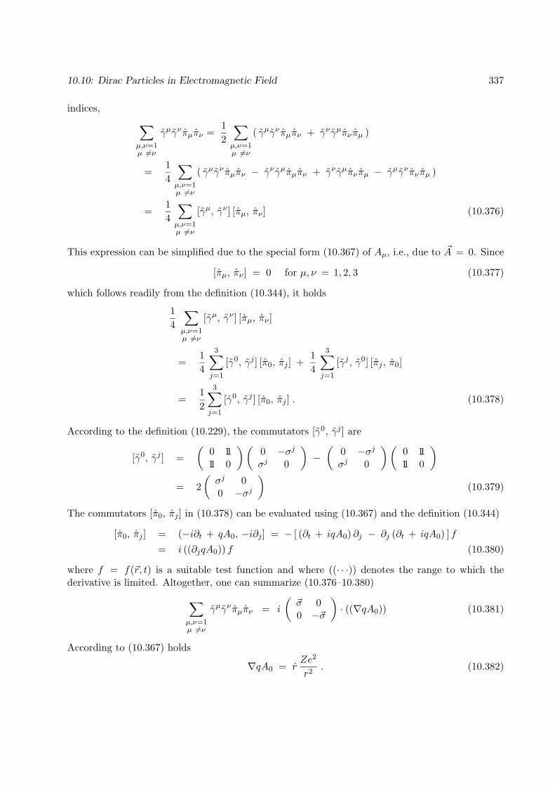
10.10: Dirac Particles in Electromagnetic Field 337
indices, ∑µ,ν=1µ 6=ν
γµγν πµπν =12
∑µ,ν=1µ 6=ν
( γµγν πµπν + γν γµπν πµ )
=14
∑µ,ν=1µ 6=ν
( γµγν πµπν − γν γµπµπν + γν γµπν πµ − γµγν πν πµ )
=14
∑µ,ν=1µ 6=ν
[γµ, γν ] [πµ, πν ] (10.376)
This expression can be simplified due to the special form (10.367) of Aµ, i.e., due to ~A = 0. Since
[πµ, πν ] = 0 for µ, ν = 1, 2, 3 (10.377)
which follows readily from the definition (10.344), it holds
14
∑µ,ν=1µ 6=ν
[γµ, γν ] [πµ, πν ]
=14
3∑j=1
[γ0, γj ] [π0, πj ] +14
3∑j=1
[γj , γ0] [πj , π0]
=12
3∑j=1
[γ0, γj ] [π0, πj ] . (10.378)
According to the definition (10.229), the commutators [γ0, γj ] are
[γ0, γj ] =(
0 1111 0
)(0 −σjσj 0
)−(
0 −σjσj 0
)(0 1111 0
)= 2
(σj 00 −σj
)(10.379)
The commutators [π0, πj ] in (10.378) can be evaluated using (10.367) and the definition (10.344)
[π0, πj ] = (−i∂t + qA0, −i∂j ] = − [ (∂t + iqA0) ∂j − ∂j (∂t + iqA0) ] f= i ((∂jqA0)) f (10.380)
where f = f(~r, t) is a suitable test function and where ((· · ·)) denotes the range to which thederivative is limited. Altogether, one can summarize (10.376–10.380)∑
µ,ν=1µ 6=ν
γµγν πµπν = i
(~σ 00 −~σ
)· ((∇qA0)) (10.381)
According to (10.367) holds
∇qA0 = rZe2
r2. (10.382)

338 Relativistic Quantum Mechanics
where r = ~r/|~r| is a unit vector. Combining this result with (10.381), (10.374), (10.375) the‘squared’ Dirac equation (10.368) reads[
−(∂t − i
Ze2
r
)2
+ ∇2 + i
(~σ · r 0
0 −~σ · r
)Ze2
r2− m2
]Ψ(xµ) = 0 (10.383)
We seek stationary solutions of this equation. Such solutions are of the form
Ψ(xµ) = Φ(~r) e−iεt . (10.384)
ε can be interpreted as the energy of the stationary state and, hence, it is this quantity that wewant to determine. Insertion of (10.384) into (10.383) yields the purely spatial four-dimensionaldifferential equation[(
ε +Ze2
r
)2
+ ∇2 + i
(~σ · r 0
0 −~σ · r
)Ze2
r2− m2
]Φ(~r) = 0 . (10.385)
We split the wave function into two spin-12 components
Ψ(~r) =(φ+(~r)φ−(~r)
)(10.386)
and obtain for the separate components φ±(~r)[(ε +
Ze2
r
)2
+ ∇2 ± i ~σ · r Ze2
r2− m2
]φ±(~r) = 0 . (10.387)
The expression (10.189) for the Laplacian and expansion of the term (· · ·)2 result in the two-dimensional equation[
∂2r −
L2 − Z2e4 ∓ i~σ · r Ze2
r2+
2Ze2ε
r+ ε2 − m2
]r φ±(~r) = 0 . (10.388)
Except for the term i~σ · r this equation is identical to that posed by the one-dimensional Klein-Gordon equation for pionic atoms (10.191) solved in Sect. 10.6. In the latter case, a solution ofthe form ∼ Y`m(r) can be obtained. The term i~σ · r, however, is genuinely two-dimensional and, infact, couples the orbital angular momentum of the electron to its spin- 1
2. Accordingly, we express
the solution of (10.388) in terms of states introduced in Sect. 6.5 which describe the coupling oforbital angular momentum and spin
(Yjm(j − 12, 1
2|r),Yjm(j + 1
2, 1
2|r) ) ,
j = 12, 3
2. . . ; m = −j, −j + 1, . . .+ j (10.389)
According to the results in Sect. 6.5 the operator i~σ · r is block-diagonal in this basis such that onlythe states for identical j, m values are coupled, i.e., only the two states Yjm(j − 1
2, 1
2|r), Yjm(j +
12, 1
2|r) as given in (6.147, 6.148). We note that these states are also eigenstates of the angular

10.10: Dirac Particles in Electromagnetic Field 339
momentum operator L2 [cf. (6.151]. We select, therefore, a specific pair of total spin-orbital angularmomentum quantum numbers j, m and expand
φ±(~r) =h±(r)rYjm(j − 1
2, 1
2|r) +
g±(r)rYjm(j + 1
2, 1
2|r) (10.390)
Using~σ · rYjm(j ± 1
2, 1
2|r) = −Yjm(j ∓ 1
2, 1
2|r) (10.391)
derived in Sect. 6.5 [c.f. (6.186)], property (6.151), which states that the states Yjm(j ± 12, 1
2|r) are
eigenfunctions of L2, together with the orthonormality of these two states leads to the coupleddifferential equation[(
∂2r +
2Ze2ε
r+ ε2 − m
) ( 1 0
0 1
)(10.392)
− 1r2
((j − 1
2)(j + 1
2) − Z2e4 ±iZe2
±i Ze2 (j + 12)(j + 3
2) − Z2e4
)](h±(r)g±(r)
)= 0 .
We seek to bring (10.392) into diagonal form. Any similarity transformation leaves the first term in(10.392), involving the 2× 2 unit matrix, unaltered. However, such transformation can be chosenas to diagonalize the second term. Since, in the present treatment, we want to determine solely thespectrum, not the wave functions, we require only the eigenvalues of the matrices
B± =
((j − 1
2)(j + 1
2) − Z2e4 ±iZe2
±i Ze2 (j + 12)(j + 3
2) − Z2e4
), (10.393)
but do not explicitly consider further the wavefunctions. Obviously, the eigenvalues are independentof m. The two eigenvalues of both matrices are identical and can be written in the form
λ1(j) [λ1(j) + 1] and λ2(j) [λ2(j) + 1] (10.394)
where
λ1(j) =√
(j + 12)2 − Z2e4 (10.395)
λ2(j) =√
(j + 12)2 − Z2e4 − 1 (10.396)
Equation (10.392) reads then in the diagonal representation(∂2r −
λ1,2(j)[λ1,2(j) + 1)r2
+2εZe2
r+ ε2 − m2
)f1,2(r) = 0 (10.397)
This equation is identical to the Klein-Gordon equation for pionic atoms written in the form(10.200), except for the slight difference in the expression of λ1,2(j) as given by (10.395, 10.396)and (10.199), namely, the missing additive term − 1
2, the values of the argument of λ1,2(j) being
j = 12, 3
2, . . . rather than ` = 0, 1, . . . as in the case of pionic atoms, and except for the fact that
we have two sets of values for λ1,2(j), namely, λ1(j) and λ2(j).. We can, hence, conclude that the
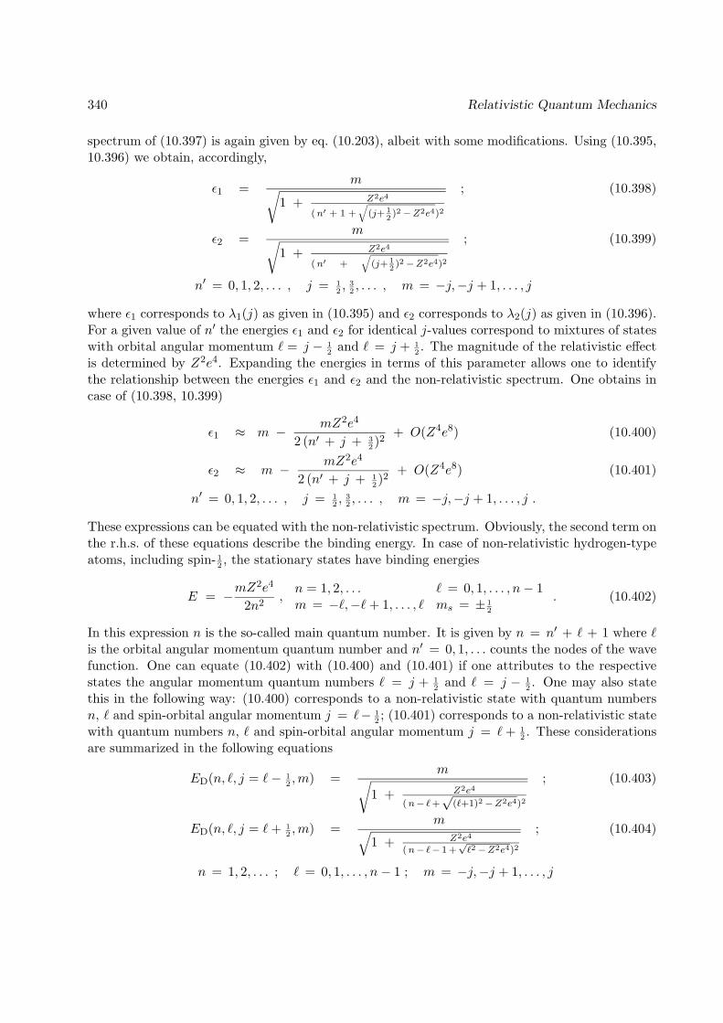
340 Relativistic Quantum Mechanics
spectrum of (10.397) is again given by eq. (10.203), albeit with some modifications. Using (10.395,10.396) we obtain, accordingly,
ε1 =m√
1 + Z2e4
(n′ + 1 +√
(j+ 12
)2−Z2e4)2
; (10.398)
ε2 =m√
1 + Z2e4
(n′ +√
(j+ 12
)2−Z2e4)2
; (10.399)
n′ = 0, 1, 2, . . . , j = 12, 3
2, . . . , m = −j,−j + 1, . . . , j
where ε1 corresponds to λ1(j) as given in (10.395) and ε2 corresponds to λ2(j) as given in (10.396).For a given value of n′ the energies ε1 and ε2 for identical j-values correspond to mixtures of stateswith orbital angular momentum ` = j − 1
2and ` = j + 1
2. The magnitude of the relativistic effect
is determined by Z2e4. Expanding the energies in terms of this parameter allows one to identifythe relationship between the energies ε1 and ε2 and the non-relativistic spectrum. One obtains incase of (10.398, 10.399)
ε1 ≈ m − mZ2e4
2 (n′ + j + 32)2
+ O(Z4e8) (10.400)
ε2 ≈ m − mZ2e4
2 (n′ + j + 12)2
+ O(Z4e8) (10.401)
n′ = 0, 1, 2, . . . , j = 12, 3
2, . . . , m = −j,−j + 1, . . . , j .
These expressions can be equated with the non-relativistic spectrum. Obviously, the second term onthe r.h.s. of these equations describe the binding energy. In case of non-relativistic hydrogen-typeatoms, including spin- 1
2, the stationary states have binding energies
E = −mZ2e4
2n2,n = 1, 2, . . . ` = 0, 1, . . . , n− 1m = −`,−`+ 1, . . . , ` ms = ± 1
2
. (10.402)
In this expression n is the so-called main quantum number. It is given by n = n′ + ` + 1 where `is the orbital angular momentum quantum number and n′ = 0, 1, . . . counts the nodes of the wavefunction. One can equate (10.402) with (10.400) and (10.401) if one attributes to the respectivestates the angular momentum quantum numbers ` = j + 1
2and ` = j − 1
2. One may also state
this in the following way: (10.400) corresponds to a non-relativistic state with quantum numbersn, ` and spin-orbital angular momentum j = `− 1
2; (10.401) corresponds to a non-relativistic state
with quantum numbers n, ` and spin-orbital angular momentum j = `+ 12. These considerations
are summarized in the following equations
ED(n, `, j = `− 12,m) =
m√1 + Z2e4
(n− `+√
(`+1)2−Z2e4)2
; (10.403)
ED(n, `, j = `+ 12,m) =
m√1 + Z2e4
(n− `− 1 +√`2−Z2e4)2
; (10.404)
n = 1, 2, . . . ; ` = 0, 1, . . . , n− 1 ; m = −j,−j + 1, . . . , j

10.10: Dirac Particles in Electromagnetic Field 341
main orbital spin- non-rel. rel.spectr. quantum angular orbital binding binding
notation number mom. ang. mom. energy / eV energy / eVn ` j Eq. (10.402) Eq. (10.405 )
1s 12
1 0 12 -13.60583 -13.60601
2s 12
2 0 12 -3.40146 -3.40151
2p 12
2 1 12 ⇑ ⇑
2p 32
2 1 32 ⇑ - 3.40147
3s 12
3 0 12 -1.51176 -1.551178
3p 12
3 1 12 ⇑ ⇑
3p 32
3 1 32 ⇑ - 1.551177
3d 32
3 2 32 ⇑ ⇑
3d 52
3 2 52 ⇑ - 1.551176
Table 10.2:Binding energies for the hydrogen (Z = 1) atom. Degeneracies are denoted by ⇑. The energieswere evaluated with m = 511.0041 keV and e2 = 1/137.036 by means of Eqs. (10.402, 10.405).
One can combine the expressions (10.403, 10.404) finally into the single formula
ED(n, `, j,m) =
m√1 + Z2e4
(n− j− 12
+√
(j+ 12
)2−Z2e4)2
n = 1, 2, . . .` = 0, 1, . . . , n− 1
j =
12
for ` = 0`± 1
2otherwise
m = −j,−j + 1, . . . , j(10.405)
In order to demonstrate relativistic effects in the spectrum of the hydrogen atom we comparein Table 10.2 the non-relativistic [cf. (10.402)] and the relativistic [cf. (10.405)] spectrum of thehydrogen atom. The table entries demonstrate that the energies as given by the expression (10.405)in terms of the non-relativistic quantum numbers n, ` relate closely to the corresponding non-relativistic states, in fact, the non-relativistic and relativistic energies are hardly discernible. Thereason is that the mean kinetic energy of the electron in the hydrogen atom, is in the range of10 eV, i.e., much less than the rest mass of the electron (511 keV). However, in case of heaviernuclei the kinetic energy of bound electrons in the ground state scales with the nuclear charge Zlike Z2 such that in case Z = 100 the kinetic energy is of the order of the rest mass and relativisticeffects become important. This is clearly demonstrated by the comparision of non-relativistic andrelativistic spectra of a hydrogen-type atom with Z = 100 in Table 10.3.Of particular interest is the effect of spin-orbit coupling which removes, for example, the non-relativistic degeneracy for the six 2p states of the hydrogen atom: in the present, i.e., relativistic,case these six states are split into energetically different 2p 1
2and 2p 3
2states. The 2p 1
2states with
j = 12 involve two degenerate states corresponding to Y 1
2m(1, 1
2|r) for m = ± 1
2, the 2p 3
2states with
j = 32
involve four degenerate states corresponding to Y 32m(1, 1
2|r) for m = ± 1
2, ± 3
2.

342 Relativistic Quantum Mechanics
main orbital spin- non-rel. rel.spectr. quantum angular orbital binding binding
notation number mom. ang. mom. energy / keV energy / keVn ` j Eq. (10.402) Eq. (10.405 )
1s 12
1 0 12 -136.1 -161.6
2s 12
2 0 12 -34.0 -42.1
2p 12
2 1 12 ⇑ ⇑
2p 32
2 1 32 ⇑ - 35.2
3s 12
3 0 12 -15.1 -17.9
3p 12
3 1 12 ⇑ ⇑
3p 32
3 1 32 ⇑ - 15.8
3d 32
3 2 32 ⇑ ⇑
3d 52
3 2 52 ⇑ - 15.3
Table 10.3:Binding energies for the hydrogen-type (Z = 100) atom. Degeneracies are denoted by ⇑. Theenergies were evaluated with m = 511.0041 keV and e2 = 1/137.036 by means of Eqs. (10.402,10.405).
In order to investigate further the deviation between relativistic and non-relativistic spectra ofhydrogen-type atoms we expand the expression (10.405) to order O(Z4e8). Introducing α = Z2e4
and β = j + 12 (10.405) reads
1√1 + α
(n−β+√β2−α)2
(10.406)
The expansion (10.206) provides in the present case
ED(n, `, j,m) ≈ m − mZ2e4
2n2− mZ4e8
2n3
[1
j + 12
− 34n
]+ O(Z6e12) . (10.407)
This expression allows one, for example, to estimate the difference between the energies of thestates 2p 3
2and 2p 1
2(cf. Tables 10.2,10.3). It holds for n = 2 and j = 3
2 ,12
E (2p 32)− E (2p 1
2) ≈ −mZ
4e8
2 · 23
[12− 1
]=
mZ4e8
32. (10.408)
Radial Dirac Equation
We want to determine now the wave functions for the stationary states of a Dirac particle in a4-vector potential
Aµ = (V (r), 0, 0, 0) (10.409)
where V (r) is spherically symmetric. An example for such potential is the Coulomb potentialV (r) = −Ze2/r considered further below. We assume for the wave function the stationary state

10.10: Dirac Particles in Electromagnetic Field 343
form
Ψ(xµ) = e−iεt(
Φ(~r)X (~r)
), (10.410)
where Φ(~r), X (~r) ∈ C2 describe the spatial and spin- 1
2degrees of freedom, but are time-
independent. The Dirac equation reads then, according to (10.232, 10.345),
~σ · ~p X + mΦ + V (r) Φ = εΦ (10.411)~σ · ~p Φ − mX + V (r)X = εX (10.412)
In this equation a coupling between the wave functions Φ(~r) and X (~r) arises due to the term ~σ · ~p.This term has been discussed in detail in Sect. 6.5 [see, in particular, pp. 168]: the term is a scalar(rank zero tensor) in the space of the spin-angular momentum states Yjm(j ± 1
2, 1
2|r) introduced in
Sect. 6.5, i.e., the term is block-diagonal in the space spanned by the states Yjm(j± 12, 1
2|r) and does
not couple states with different j,m-values; ~σ · ~p has odd parity and it holds [c.f. (6.197, 6.198)]
~σ · ~p f(r)Yjm(j + 12, 1
2|r) = i
[∂r +
j + 32
r
]f(r)Yjm(j − 1
2, 1
2|r)
(10.413)
~σ · ~p g(r)Yjm(j − 12, 1
2|r) = i
[∂r +
12 − jr
]g(r)Yjm(j + 1
2, 1
2|r) .
(10.414)
These equations can be brought into a more symmetric form using
∂r +1r
=1r∂r r
which allows one to write (10.413, 10.414)
~σ · ~p rf(r)Yjm(j + 12, 1
2|r) = i
[∂r +
j + 12
r
]r f(r)Yjm(j − 1
2, 1
2|r)
(10.415)
~σ · ~p rg(r)Yjm(j − 12, 1
2|r) = i
[∂r −
j + 12
r
]r g(r)Yjm(j + 1
2, 1
2|r) .
(10.416)
The differential equations (10.411, 10.412) are four-dimensional with ~r-dependent wave functions.The arguments above allow one to eliminate the angular dependence by expanding Φ(~r) and X (~r)in terms of Yjm(j + 1
2, 1
2|r) and Yjm(j − 1
2, 1
2|r), i.e.,
Φ(~r)
X (~r)
=
a(r)rYjm(j + 1
2, 1
2|r) +
b(r)rYjm(j − 1
2, 1
2|r)
c(r)rYjm(j + 1
2, 1
2|r) +
d(r)rYjm(j − 1
2, 1
2|r)
. (10.417)

344 Relativistic Quantum Mechanics
In general, such expansion must include states with all possible j,m values. Presently, we considerthe case that only states for one specific j,m pair contribute. Inserting (10.417) into (10.411,10.412), using (10.415, 10.416), the orthonormality property (6.157), and multiplying by r resultsin the following two independent pairs of coupled differential equations
i
[∂r −
j + 12
r
]d(r) + [ m + V (r) − ε ] a(r) = 0
i
[∂r +
j + 12
r
]a(r) + [−m + V (r) − ε ] d(r) = 0 (10.418)
and
i
[∂r +
j + 12
r
]c(r) + [ m + V (r) − ε ] b(r) = 0
i
[∂r −
j + 12
r
]b(r) + [−m + V (r) − ε ] c(r) = 0 . (10.419)
Obviously, only a(r), d(r) are coupled and b(r), c(r) are coupled. Accordingly, there exist twoindependent solutions (10.417) of the form Φ(~r)
X (~r)
=
if1(r)rYjm(j + 1
2, 1
2|r)
− g1(r)rYjm(j − 1
2, 1
2|r)
(10.420)
(Φ(~r)
X (~r)
)=
if2(r)rYjm(j − 1
2, 1
2|r)
− g2(r)rYjm(j + 1
2, 1
2|r)
(10.421)
where the factors i and −1 have been introduced for convenience. According to (10.418) holds forf1(r), g1(r) [
∂r −j + 1
2
r
]g1(r) + [ ε − m − V (r) ] f1(r) = 0
[∂r +
j + 12
r
]f1(r) − [ ε + m − V (r) ] g1(r) = 0 (10.422)
and for f2(r), g2(r) [∂r +
j + 12
r
]g2(r) + [ ε − m − V (r) ] f2(r) = 0
[∂r −
j + 12
r
]f2(r) − [ ε + m − V (r) ] g2(r) = 0 (10.423)
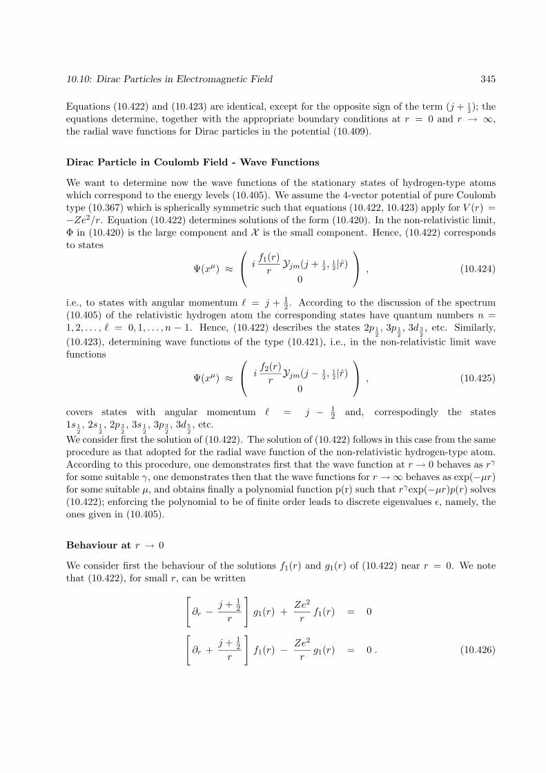
10.10: Dirac Particles in Electromagnetic Field 345
Equations (10.422) and (10.423) are identical, except for the opposite sign of the term (j + 12); the
equations determine, together with the appropriate boundary conditions at r = 0 and r → ∞,the radial wave functions for Dirac particles in the potential (10.409).
Dirac Particle in Coulomb Field - Wave Functions
We want to determine now the wave functions of the stationary states of hydrogen-type atomswhich correspond to the energy levels (10.405). We assume the 4-vector potential of pure Coulombtype (10.367) which is spherically symmetric such that equations (10.422, 10.423) apply for V (r) =−Ze2/r. Equation (10.422) determines solutions of the form (10.420). In the non-relativistic limit,Φ in (10.420) is the large component and X is the small component. Hence, (10.422) correspondsto states
Ψ(xµ) ≈
if1(r)rYjm(j + 1
2, 1
2|r)
0
, (10.424)
i.e., to states with angular momentum ` = j + 12 . According to the discussion of the spectrum
(10.405) of the relativistic hydrogen atom the corresponding states have quantum numbers n =1, 2, . . . , ` = 0, 1, . . . , n − 1. Hence, (10.422) describes the states 2p 1
2, 3p 1
2, 3d 3
2, etc. Similarly,
(10.423), determining wave functions of the type (10.421), i.e., in the non-relativistic limit wavefunctions
Ψ(xµ) ≈
if2(r)rYjm(j − 1
2, 1
2|r)
0
, (10.425)
covers states with angular momentum ` = j − 12 and, correspodingly the states
1s 12, 2s 1
2, 2p 3
2, 3s 1
2, 3p 3
2, 3d 5
2, etc.
We consider first the solution of (10.422). The solution of (10.422) follows in this case from the sameprocedure as that adopted for the radial wave function of the non-relativistic hydrogen-type atom.According to this procedure, one demonstrates first that the wave function at r → 0 behaves as rγ
for some suitable γ, one demonstrates then that the wave functions for r →∞ behaves as exp(−µr)for some suitable µ, and obtains finally a polynomial function p(r) such that rγexp(−µr)p(r) solves(10.422); enforcing the polynomial to be of finite order leads to discrete eigenvalues ε, namely, theones given in (10.405).
Behaviour at r → 0
We consider first the behaviour of the solutions f1(r) and g1(r) of (10.422) near r = 0. We notethat (10.422), for small r, can be written[
∂r −j + 1
2
r
]g1(r) +
Ze2
rf1(r) = 0
[∂r +
j + 12
r
]f1(r) − Ze2
rg1(r) = 0 . (10.426)
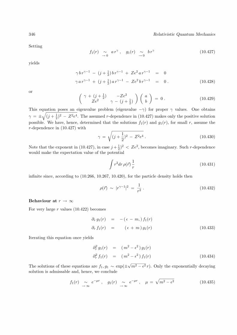
346 Relativistic Quantum Mechanics
Settingf1(r) ∼
→ 0a rγ , g1(r) ∼
→ 0b rγ (10.427)
yields
γ b rγ−1 − (j + 12) b rγ−1 + Ze2 a rγ−1 = 0
γ a rγ−1 + (j + 12) a rγ−1 − Ze2 b rγ−1 = 0 . (10.428)
or (γ + (j + 1
2) −Ze2
Ze2 γ − (j + 12)
) (ab
)= 0 . (10.429)
This equation poses an eigenvalue problem (eigenvalue −γ) for proper γ values. One obtains
γ = ±√
(j + 12)2 − Z2e4. The assumed r-dependence in (10.427) makes only the positive solution
possible. We have, hence, determined that the solutions f1(r) and g1(r), for small r, assume ther-dependence in (10.427) with
γ =
√(j +
12
)2 − Z2e4 . (10.430)
Note that the exponent in (10.427), in case j+ 12)2 < Ze2, becomes imaginary. Such r-dependence
would make the expectation value of the potential∫r2dr ρ(~r)
1r
(10.431)
infinite since, according to (10.266, 10.267, 10.420), for the particle density holds then
ρ(~r) ∼ |rγ−1|2 =1r2. (10.432)
Behaviour at r → ∞
For very large r values (10.422) becomes
∂r g1(r) = − ( ε − m, ) f1(r)
∂r f1(r) = ( ε + m ) g1(r) (10.433)
Iterating this equation once yields
∂2r g1(r) = (m2 − ε2 ) g1(r)
∂2r f1(r) = (m2 − ε2 ) f1(r) (10.434)
The solutions of these equations are f1, g1 ∼ exp(±√m2 − ε2 r). Only the exponentially decaying
solution is admissable and, hence, we conclude
f1(r) ∼→∞
e−µr , g1(r) ∼→∞
e−µr , µ =√m2 − ε2 (10.435)

10.10: Dirac Particles in Electromagnetic Field 347
For bound states holds ε < m and, hence, µ is real. Let us consider then for the solution of (10.434)
f1(r) =√m+ ε a e−µ r , g1(r) = −
√m− ε a e−µr . (10.436)
Insertion into (10.434) results in
(m− ε)√m+ ε a − (m− ε)
√m+ ε a = 0
(m+ ε)√m− ε a − (m+ ε)
√m− ε a = 0 (10.437)
which is obviously correct.
Solution of the Radial Dirac Equation for a Coulomb Potential
To solve (10.422) for the Coulomb potential V (r) = −Ze2/r We assume a form for the solutionwhich is adopted to the asymptotic solution (10.436). Accordingly, we set
f1(r) =√m+ ε e−µr f1(r) (10.438)
g1(r) = −√m− ε e−µr g1(r) (10.439)
where µ is given in (10.435 ). Equation (10.422 ) leads to
−√m− ε [∂r −
j + 12
r] g1 +
√m+ ε
Ze2
rf1 +
(m− ε)√m+ ε g1 − (m− ε)
√m+ ε f1 = 0 (10.440)
√m+ ε [∂r +
j + 12
r] f1 +
√m− ε Ze
2
rg1 −
(m+ ε)√m− εf1 + (m+ ε)
√m− εg1 = 0 (10.441)
The last two terms on the l.h.s. of both (10.440) and (10.441) correspond to (10.437) where theycancelled in case f1 = g1 = a. In the present case the functions f1 and g1 cannot be chosenidentical due to the terms in the differential equations contributing for finite r. However, withoutloss of generality we can choose
f1(r) = φ1(r) + φ2(r) , g1(r) = φ1(r) − φ2(r) (10.442)
which leads to a partial cancellation of the asymptotically dominant terms. We also introduce thenew variable
ρ = 2µ r . (10.443)
From this results after a little algebra
[∂ρ −j + 1
2
ρ] (φ1 − φ2) −
√m+ ε
m− εZe2
ρ(φ1 + φ2) + φ2 = 0 (10.444)
[∂ρ +j + 1
2
ρ] (φ1 + φ2) +
√m− εm+ ε
Ze2
ρ(φ1 − φ2) − φ2 = 0 . (10.445)

348 Relativistic Quantum Mechanics
Addition and subtraction of these equations leads finally to the following two coupled differentialequations for φ1 and φ2
∂ρφ1 +j + 1
2
ρφ2 −
εZe2
√m2 − ε2 ρ
φ1 −mZe2
√m2 − ε2 ρ
φ2 = 0 (10.446)
∂ρφ2 +j + 1
2
ρφ1 +
mZe2
√m2 − ε2 ρ
φ1 +εZe2
√m2 − ε2 ρ
φ2 − φ2 = 0 (10.447)
We seek solutions of (10.446 , 10.447) of the form
φ1(ρ) = ργn′∑s=0
αs ρ2 (10.448)
φ2(ρ) = ργn′∑s=0
βs ρ2 (10.449)
for γ given in (10.430) which conform to the proper r → 0 behaviour determined above [c.f.(10.426–10.430)]. Inserting (10.448, 10.449) into (10.446, 10.447) leads to
∑s
[(s+ γ)αs + (j + 1
2)βs −εZe2
√m2 − ε2
αs
− mZe2
√m2 − ε2
βs
]ρs+γ−1 = 0 (10.450)
∑s
[(s+ γ)β2 + (j + 1
2)αs +mZe2
√m2 − ε2
αs
+εZe2
√m2 − ε2
βs − βs−1
]= 0 (10.451)
From (10.450) follows
αsβs
=mZe2√m2−ε2 − (j + 1
2)
s + γ − εZe2√m2−ε2
. (10.452)
From (10.451) follows
βs−1 =(s + γ +
εZe2
√m2 − ε2
)βs +
m2Z2e4
m2−ε2 − (j + 12)2
s + γ − εZe2√m2−ε2
βs
=(s+ γ)2 + Z2e4 − (j + 1
2)2
s + γ − εZe2√m2−ε2
βs . (10.453)
Using (10.430) one can write this
βs =s + γ − εZe2√
m2−ε2
s (s + 2γ)βs−1 . (10.454)

10.10: Dirac Particles in Electromagnetic Field 349
Defining
so =εZe2
√m2 − ε2
− γ (10.455)
one obtains
βs =s− so
s(s+ 2γ)βs−1
=(s− 1− so)(s− so)
(s− 1)s (s− 1 + 2γ)(s+ 2γ)βs−2
...
=(1− so)(2− so) . . . (s− so)
s! (2γ + 1)(2γ + 2) · · · (2γ + s)β0 (10.456)
From (10.452) follows
αs =j + 1
2 −mZe2√m2−ε2
so
(−so)(1− so)(2− so) . . . (s− so)s! (2γ + 1)(2γ + 2) · · · (2γ + s)
β0 (10.457)
One can relate the polynomials φ1(ρ) and φ2(ρ) defined through (10.448, 10.449) and (10.456,10.457) with the confluent hypergeometric functions
F (a, c;x) = 1 +a
cx +
a(a+ 1)c(c+ 1)
x2
2!+ . . . (10.458)
or, equivalently, with the associated Laguerre polynomials
L(α)n = F (−n, α+ 1, x) . (10.459)
It holds
φ1(ρ) = β0
j + 12 −
mZe2√m2−ε2
soργ F (−so, 2γ + 1; ρ) (10.460)
φ2(ρ) = β0 ργ F (1− so, 2γ + 1; ρ) . (10.461)
In order that the wave functions remain normalizable the power series (10.448, 10.449) must be offinite order. This requires that all coefficients αs and βs must vanish for s ≥ n′ for some n′ ∈ N.The expressions (10.456) and (10.457) for βs and αs imply that so must then be an integer, i.e.,so = n′. According to the definitions (10.430, 10.455) this confinement of so implies discrete valuesfor ε, namely,
ε(n′) =m√
1 + Z2e4
(n′+√
(j+ 12
)2−Z2e4)2
, n′ = 0, 1, 2, . . . (10.462)
This expression agrees with the spectrum of relativistic hydrogen-type atoms derived above andgiven by (10.405). Comparision with (10.405) allows one to identify n′ = n− j + 1
2 which, in fact,is an integer. For example, for the states 2p 1
2, 3p 1
2, 3d 3
2holds n′ = 1, 2, 1. We can, hence, conclude
that the polynomials in (10.461 for ε values given by (10.405) and the ensuing so values ( 10.455)are finite.

350 Relativistic Quantum Mechanics
Altogether we have determined the stationary states of the type (10.421) with radial wave functionsf1(r), g1(r) determined by (10.438, 10.439), (10.442), and (10.460, 10.461). The coefficients β0 in(10.460, 10.461) are to be chosen to satisfy a normalization condition and to assign an overallphase. Due to the form (10.410) of the stationary state wave function the density ρ(xµ) of thestates under consideration, given by expression (10.267), is time-independent. The normalizationintegral is then ∫ ∞
0r2dr
∫ π
0sin θdθ
∫ 2π
0dφ (|Φ(~r)|2 + |X (~r)|2) = 1 (10.463)
where Φ and X , as in (10.421), are two-dimensional vectors determined through the explicit formof the spin-orbital angular momentum states Yjm(j± 1
2 ,12 |r) in (6.147, 6.148). The orthonormality
properties (6.157, 6.158) of the latter states absorb the angular integral in (10.463) and yield [notethe 1/r factor in (10.421)] ∫ ∞
0dr (|f1(r)|2 + |g1(r)|2) = 1 (10.464)
The evaluation of the integrals, which involve the confluent hypergeometric functions in (10.460,10.461), can follow the procedure adopted for the wave functions of the non-relativistic hydrogenatom and will not be carried out here.The wave functions (10.421) correspond to non-relativistic states with orbital angular momentum` = j + 1
2 . They are described through quantum numbers n, j, ` = j + 12 ,m. The complete wave
function is given by the following set of formulas
Ψ(n, j, ` = j + 12 ,m|x
µ) = e−iεt
(iF1(r)Yj,m(j + 1
2 ,12 |r)
G1(r)Yj,m(j − 12 ,
12 |r)
)(10.465)
F1(r) = F−(κ|r) , G1(r) = F+(κ|r) , κ = j + 12 (10.466)
where2
F±(κ|r) = ∓N (2µr)γ−1e−µr[
(n′ + γ)mε
− κ
]F (−n′, 2γ + 1; 2µr)
± n′F (1− n′, 2γ + 1; 2µr)
(10.467)
N =(2µ)
32
Γ(2γ + 1)
√√√√ m∓ ε)Γ(2γ + n′ + 1)
4m (n′+γ)mε
((n′+γ)m
ε − κ)n′!
(10.468)
and
µ =√
(m− ε)(m+ ε)
γ =√
(j + 12)2 − Z2e4
n′ = n − j − 12
ε =m√
1 + Z2e4
(n′+γ)2
. (10.469)
2This formula has been adapted from ”Relativistic Quantum Mechanics” by W. Greiner, (Springer, Berlin, 1990),Sect. 9.6.
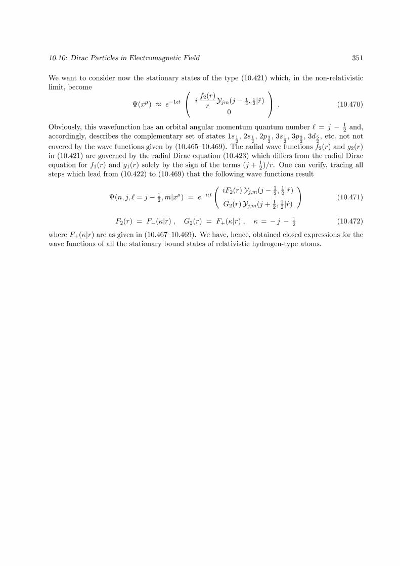
10.10: Dirac Particles in Electromagnetic Field 351
We want to consider now the stationary states of the type (10.421) which, in the non-relativisticlimit, become
Ψ(xµ) ≈ e−1εt
if2(r)rYjm(j − 1
2, 1
2|r)
0
. (10.470)
Obviously, this wavefunction has an orbital angular momentum quantum number ` = j − 12 and,
accordingly, describes the complementary set of states 1s 12, 2s 1
2, 2p 3
2, 3s 1
2, 3p 3
2, 3d 5
2, etc. not not
covered by the wave functions given by (10.465–10.469). The radial wave functions f2(r) and g2(r)in (10.421) are governed by the radial Dirac equation (10.423) which differs from the radial Diracequation for f1(r) and g1(r) solely by the sign of the terms (j + 1
2)/r. One can verify, tracing allsteps which lead from (10.422) to (10.469) that the following wave functions result
Ψ(n, j, ` = j − 12 ,m|x
µ) = e−iεt
(iF2(r)Yj,m(j − 1
2 ,12 |r)
G2(r)Yj,m(j + 12 ,
12 |r)
)(10.471)
F2(r) = F−(κ|r) , G2(r) = F+(κ|r) , κ = − j − 12 (10.472)
where F±(κ|r) are as given in (10.467–10.469). We have, hence, obtained closed expressions for thewave functions of all the stationary bound states of relativistic hydrogen-type atoms.

352 Relativistic Quantum Mechanics

Chapter 11
Spinor Formulation of RelativisticQuantum Mechanics
11.1 The Lorentz Transformation of the Dirac Bispinor
We will provide in the following a new formulation of the Dirac equation in the chiral representationdefined through (10.225–10.229). Starting point is the Lorentz transformation S(~w, ~ϑ) for thebispinor wave function Ψ in the chiral representation as given by (10.262). This transformationcan be written
S(~z) =(a(~z) 0
0 b(~z)
)(11.1)
a(~z) = exp(
12~z · ~σ
)(11.2)
b(~z) = exp(−1
2~z ∗ · ~σ
)(11.3)
~z = ~w − i ~ϑ . (11.4)
We have altered here slightly our notation of S(~w, ~ϑ), expressing its dependence on ~w, ~ϑ througha complex variable ~z, ~z ∈ C3.Because of its block-diagonal form each of the diagonal components of S(~z), i.e., a(~z) and b(~z),must be two-dimensional irreducible representations of the Lorentz group. This fact is remarkablesince it implies that the representations provided through a(~z) and b(~z) are of lower dimension thenthe four-dimensional natural representation1 L(~w, ~ϑ)µν . The lower dimensionality of a(~z) and b(~z)implies, in a sense, that the corresponding representation of the Lorentz group is more basic thanthe natural representation and may serve as a building block for all representations, in particular,may be exploited to express the Lorentz-invariant equations of relativistic quantum mechanics.This is, indeed, what will be achieved in the following.We will proceed by building as much as possible on the results obtained sofar in the chiral repre-sentation of the Dirac equation. We will characterize the space on which the transformations a(~z)
1We will see below that the representations a(~z) and b(~z) are, in fact, isomorphic to the natural representation,
i.e., different L(~w, ~ϑ)µν correspond to different a(~z) and b(~z).
353
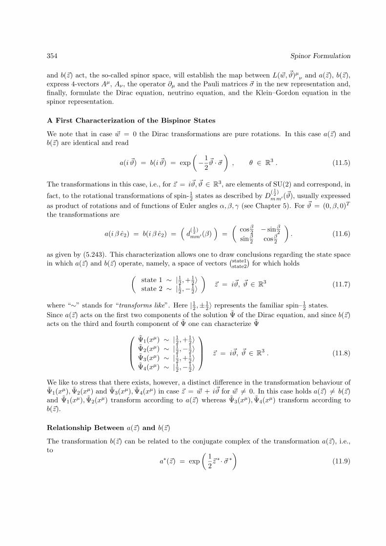
354 Spinor Formulation
and b(~z) act, the so-called spinor space, will establish the map between L(~w, ~ϑ)µν and a(~z), b(~z),express 4-vectors Aµ, Aν , the operator ∂µ and the Pauli matrices ~σ in the new representation and,finally, formulate the Dirac equation, neutrino equation, and the Klein–Gordon equation in thespinor representation.
A First Characterization of the Bispinor States
We note that in case ~w = 0 the Dirac transformations are pure rotations. In this case a(~z) andb(~z) are identical and read
a(i ~ϑ) = b(i ~ϑ) = exp(−1
2~ϑ · ~σ
), θ ∈ R3 . (11.5)
The transformations in this case, i.e., for ~z = i~ϑ, ~ϑ ∈ R3, are elements of SU(2) and correspond, in
fact, to the rotational transformations of spin-12 states as described by D
( 12
)
mm′(~ϑ), usually expressedas product of rotations and of functions of Euler angles α, β, γ (see Chapter 5). For ~ϑ = (0, β, 0)T
the transformations are
a(i β e2) = b(i β e2) =(d
( 12
)
mm′(β))
=(
cosβ2 − sinβ2sinβ2 cosβ2
). (11.6)
as given by (5.243). This characterization allows one to draw conclusions regarding the state spacein which a(~z) and b(~z) operate, namely, a space of vectors
(state1state2
)for which holds(
state 1 ∼ |12 ,+12〉
state 2 ∼ |12 ,−12〉
)~z = i~ϑ, ~ϑ ∈ R3 (11.7)
where “∼” stands for “transforms like”. Here |12 ,±12〉 represents the familiar spin–1
2 states.Since a(~z) acts on the first two components of the solution Ψ of the Dirac equation, and since b(~z)acts on the third and fourth component of Ψ one can characterize Ψ
Ψ1(xµ) ∼ |12 ,+12〉
Ψ2(xµ) ∼ |12 ,−12〉
Ψ3(xµ) ∼ |12 ,+12〉
Ψ4(xµ) ∼ |12 ,−12〉
~z = i~ϑ, ~ϑ ∈ R3 . (11.8)
We like to stress that there exists, however, a distinct difference in the transformation behaviour ofΨ1(xµ), Ψ2(xµ) and Ψ3(xµ), Ψ4(xµ) in case ~z = ~w + i~ϑ for ~w 6= 0. In this case holds a(~z) 6= b(~z)and Ψ1(xµ), Ψ2(xµ) transform according to a(~z) whereas Ψ3(xµ), Ψ4(xµ) transform according tob(~z).
Relationship Between a(~z) and b(~z)
The transformation b(~z) can be related to the conjugate complex of the transformation a(~z), i.e.,to
a∗(~z) = exp(
12~z ∗ · ~σ ∗
)(11.9)

11.1: Lorentz Transformation of Dirac Bispinor 355
where ~σ ∗ = (σ∗1, σ∗2, σ∗3). One can readily verify [c.f. (5.224)]
σ1 = σ∗1 , σ2 = −σ∗2 , σ3 = σ∗3 . (11.10)
From this one can deriveb(~z) = ε a∗(~z) ε−1 (11.11)
where
ε =(
0 1−1 0
), ε−1 =
(0 −11 0
). (11.12)
To prove (11.11) one first demonstrates that for ε and ε−1 as given in (11.12) does, in fact, holdε ε−1 = 11. One notices then, using εf(a)ε−1 = f(εaε−1),
ε a∗(~z)ε−1 = exp[
12~z ∗(ε~σ ∗ε−1
) ]. (11.13)
Explicit matrix multiplication using (5.224, 11.10, 11.12) yields
εσ1ε−1 = −σ1 = −σ∗1
εσ2ε−1 = σ2 = −σ∗2 (11.14)
εσ3ε−1 = −σ3 = −σ∗3 ,
or in shortε~σε−1 = −~σ ∗ . (11.15)
Similarly, one can showε−1~σε = −~σ ∗ , (11.16)
a result to be used further below. Hence, one can express
ε a∗(~z) ε−1 = exp(−1
2~z ∗ · ~σ
)= b(~z) . (11.17)
We conclude, therefore, that the transformation (11.1) can be written in the form
S(~z) =(a(~z) 0
0 ε a∗(~z) ε−1
)(11.18)
with a(~z) given by (11.2, 11.4) and ε, ε−1 given by (11.12). This demonstrates that a(~z) is thetransformation which characterizes both components of S(~z).
Spatial Inversion
One may question from the form of S(~z) why the Dirac equation needs to be four-dimensional,featuring the components Ψ1(xµ), Ψ2(xµ) as well as Ψ3(xµ), Ψ4(xµ) even though these pairs ofcomponents transform independently of each other. The answer lies in the necessity that applicationof spatial inversion should transform a solution of the Dirac equation into another possible solutionof the Dirac equation. The effect of inversion on Lorentz transformations is, however, that theyalter ~w into −~w, but leave rotation angles ~ϑ unaltered.

356 Spinor Formulation
Let P denote the representation of spatial inversion in the space of the wave functions Ψ. Obviously,P2 = 11, i.e., P−1 = P. The transformation S(~z) in the transformed space is then
P S(~w + i~ϑ)P = S(−~w + i~ϑ) =(b(~z) 0
0 a(~z)
), (11.19)
i.e., the transformations a(~z) and b(~z) become interchanged. This implies
P
Ψ1
Ψ2
Ψ3
Ψ4
=
Ψ3
Ψ4
Ψ1
Ψ2
. (11.20)
Obviously, the space spanned by only two of the components of Ψ is not invariant under spatialinversion and, hence, does not suffice for particles like the electron which obey inversion symmetry.However, for particles like the neutrinos which do not obey inversion symmetry two componentsof the wave function are sufficient. In fact, the Lorentz invariant equation for neutrinos is only2–dimensional.
11.2 Relationship Between the Lie Groups SL(2,C) and SO(3,1)
We have pointed out that a(i~ϑ), ~ϑ ∈ R3, which describes pure rotations, is an element of SU(2).However, a(~w + i~ϑ) for ~w 6= 0 is an element of
SL(2,C) = M, M is a complex 2× 2–matrix,det(M) = 1 . (11.21)
One can verify this by evaluating the determinant of a(~z)
det( a(~z) ) = det(e
12~z·~σ)
= etr( 12~z·~σ) = 1 (11.22)
which follows from the fact that for any complex, non-singular matrix M holds2
det(eM)
= etr(M) (11.23)
and from [c.f. (5.224)]tr(σj ) = 0 , j = 1, 2, 3 . (11.24)
Exercise 11.2.1: Show that SL(2,C) defined in (11.21) together with matrix multiplication asthe binary operation forms a group.
2The proof of this important property is straightforward in case of hermitian M (see Chapter 5). For the generalcase the proof, based on the Jordan–Chevalley theorem, can be found in G.G.A. Bauerle and E.A. de Kerf LieAlgebras, Part (Elsevier, Amsterdam, 1990), Exercise 1.10.3.

11.2: Lie Groups SL(2,C) and SO(3,1) 357
Mapping Aµ onto matrices M(Aµ)
We want to establish now the relationship between SL(2,C) and the group L↑+ of proper, or-thochronous Lorentz transformations. Starting point is a bijective map between R4 and the set oftwo-dimensional hermitian matrices defined through
M(Aµ) = σµAµ (11.25)
where
σµ =
(
1 00 1
)︸ ︷︷ ︸
σ0
,
(0 11 0
)︸ ︷︷ ︸
σ1
,
(0 −ii 0
)︸ ︷︷ ︸
σ2
,
(1 00 −1
)︸ ︷︷ ︸
σ3
. (11.26)
The quantity σµ thus defined does not transform like a covariant 4–vector. In fact, one wishesthat the definition (11.25) of the matrix M(Aµ) is independent of the frame of reference, i.e., in atransformed frame should hold
σµAµ Lρν
−→σµA
′µ . (11.27)
Straightforward transformation into another frame of reference would replace σµ by σ′µ. UsingAµ = (L−1)µνA′ν one would expect in a transformed frame to hold
σµAµ L
ρν
−→σ′µ (L−1)µν A′ν . (11.28)
Consistency of (11.28) and (11.27) requires then
Lνµσ′µ = σν (11.29)
where we used (10.76). Noting that for covariant vectors according to (10.75) holds a′ν = Lνµaµ
one realizes that σµ transforms inversely to covariant 4–vectors. We will prove below [cf. (11.135)]this transformation behaviour.M(Aµ) according to (11.25) can also be written
M(Aµ) =(A0 + A3 A1 − iA2
A1 + iA2 A0 − A3
). (11.30)
Since the components of Aµ are real, the matrix M(Aµ) is hermitian as can be seen from inspectionof (11.26) or from the fact that the matrices σ0, σ1, σ2, σ3 are hermitian. The function M(Aµ) isbijective, in fact, one can provide a simple expression for the inverse of M(Aµ)
M ′ = M(Aµ) ↔ Aµ =12
tr(M ′ σµ
). (11.31)
Exercise 11.2.2: Show that σ0, σ1, σ2, σ3 provide a linear–independent basis for the space ofhermitian 2×2–matrices. Argue why M(Aµ) = σµA
µ provides a bijective map. Demonstrate that(11.31) holds.
The following important property holds for M(Aµ)
det (M(Aµ) ) = AµAµ (11.32)
which follows directly from (11.30).

358 Spinor Formulation
Transforming the matrices M(Aµ)
We define now a transformation of the matrix M(Aµ) in the space of hermitian 2× 2–matrices
Ma−→ M ′ = aM a† , a ∈ SL(2,C) . (11.33)
This transformation conserves the hermitian property of M since
(M ′)† = ( aM a† )† = (a†)†M †a† = aM a† = M ′ (11.34)
where we used the properties M † = M and (a†)† = a. Due to det(a) = 1 the transformation(11.33) conserves the determinant of M . In fact, it holds for the matrix M ′ defined through (11.33)
det(M ′) = det( aM a† ) = det(a) det(a†) det(M)= [det(a)]2 det(M) = det(M) . (11.35)
We now apply the transformation (11.33) to M(Aµ) describing the action of the transformation interms of transformations of Aµ. In fact, for any a ∈ SL(2,C) and for any Aµ there exists an A′µ
such that
M(A′µ) = aM(Aµ) a† . (11.36)
The suitable A′µ can readily be constructed using (11.31). Accordingly, any a ∈ SL(2,C) definesthe transformation [c.f. (11.31)]
Aµa−→ A′µ =
12
tr(aM(Aµ) a†σµ
). (11.37)
Because of (11.32, 11.35) holds for this transformation
A′µA′µ = AµAµ (11.38)
which implies that (11.37) defines actually a Lorentz transformation. The linear character of thetransformation becomes apparent expressing A′µ as given in (11.37) using (11.25)
A′µ =12
tr(a σνa
†σµ
)Aν (11.39)
which allows us to express finally
A′µ = L(a)µν Aν ; L(a)µν =12
tr(a σνa
†σµ
). (11.40)
Exercise 11.2.3: Show that L(a)µν defined in (11.40) is an element of L↑+.

11.2: Lie Groups SL(2,C) and SO(3,1) 359
L(a)µν provides a homomorphism
We want to demonstrate now that the map between SL(2, C) and SO(3,1) defined through L(a)µν[cf. (11.40)] respects the group property of SL(2, C) and of SO(3,1), i.e.,
Lµρ = L(a1)µν L(a2)µρ︸ ︷︷ ︸product
in SO(3,1)
= L( a1 a2︸ ︷︷ ︸product
in SL(2,C)
)µρ (11.41)
For this purpose one writes using tr(AB) = tr(BA)
L(a1)µν L(a2)µρ =∑ν
12
tr(a1σνa
†1σµ
) 12
tr(a2σρa
†2σν
)=
∑ν
12
tr(σνa
†1σµa1
) 12
tr(a2σρa
†2σν
). (11.42)
DefiningΓ = a†1σµa1 , Γ′ = a2σρa
†2 (11.43)
and using the definition of Lµρ in (11.41) results in
Lµρ =14
∑ν,α,βγ,δ
(σν)αβΓβα Γγδ(σν)δγ =14
∑α,βγ,δ
AαβγδΓβα Γγδ (11.44)
whereAαβγδ =
∑ν
(σν)αβ(σν)δγ . (11.45)
One can demonstrate through direct evaluation
Aαβγδ =
2 α = β = γ = δ = 12 α = β = γ = δ = 22 α = γ = 1 , β = δ = 22 α = γ = 2 , β = δ = 10 else
(11.46)
which yields
Lµρ =12(
Γ11Γ′11 + Γ22Γ′22 + Γ12Γ′21 + Γ21Γ′12
)=
12
tr(
ΓΓ′)
=12
tr(a†1σµa1 a2σρa
†2
)=
12
tr(σµa1a2σρa
†2a†1
)=
12
tr(a1a2σρ(a1a2)†σµ
)= L(a1a2)µρ . (11.47)
This completes the proof of the homomorphic property of L(a)µν .

360 Spinor Formulation
Generators for SL(2, C) which correspond to ~K, ~J
The transformations a ∈ SL(2,C) as complex 2 × 2–matrices are defined through four complexor, correspondingly, eight real numbers. Because of the condition det(a) = 1 only six independentreal numbers actually suffice for the definition of a. One expects then that six generators Gj andsix real coordinates fj can be defined which allow one to represent a in the form
a = exp
6∑j=1
fjGj
. (11.48)
We want to determine now the generators of the transformation a(~z) as defined in (11.2) whichcorrespond to the generators K1,K2,K3, J1, J2, J3 of the Lorentz transformations Lµν in the naturalrepresentations, i.e., correspond to the generators given by (10.47, 10.48). To this end we considerinfinitesimal transformations and keep only terms of zero order and first order in the small variables.To obtain the generator of a(~z) corresponding to the generator K1, denoted below as κ1, we write(11.36)
M(LµνAν) = aM(Aµ) a† (11.49)
assuming (note that gµν is just the familiar Kronecker δµν)
Lµν = gµν + ε (K1)µ ν (11.50)a = 11 + ε κ1 . (11.51)
Insertion of (K1)µν as given in (10.48) yields for the l.h.s. of (11.49), noting the linearity of M(Aµ),
M(Aµ + ε (K1)µ ν Aν) = M(Aµ) + εM( (−A1,−A0, 0, 0) )= M(Aµ) − ε σ0A
1 − ε σ1A0 (11.52)
where we employed (11.25) in the last step. For the r.h.s. of (11.49) we obtain using (11.51)
( 11 + ε κ1 )M(Aµ) ( 11 + ε κ†1 )
= M(Aµ) + ε (κ1M(Aµ) + M(Aµ)κ†1 ) + O(ε2)
= M(Aµ) + ε (κ1σµ + σµκ†1 )Aµ + O(ε2) . (11.53)
Equating (11.52) and (11.53) results in the condition
σ0A1 − σ1A
0 = (κ1σµ + σµ κ†1 )Aµ . (11.54)
This reads for the four cases Aµ = (1, 0, 0, 0), Aµ = (0, 1, 0, 0), Aµ = (0, 0, 1, 0), Aµ = (0, 0, 0, 1)
−σ1 = κ1σ0 + σ0κ†1 = κ1 + κ†1 (11.55)
σ0 = κ1σ1 + σ1κ†1 (11.56)
0 = κ1σ2 + σ2κ†1 (11.57)
0 = κ1σ3 + σ3κ†1 . (11.58)
One can verify readily that
κ1 = −12σ1 (11.59)

11.3: Spinors 361
obeys these conditions. Similarly, one can show that the generators κ2, κ3 of a(~z) corresponding toK2,K3 and λ1, λ2, λ3 corresponding to J1, J2, J3 are given by
κ = −12~σ , ~λ =
i
2~σ . (11.60)
We can, hence, state that the following two transformations are equivalent
L(~w, ~ϑ) = e~w·~K + ~ϑ· ~J︸ ︷︷ ︸
∈ SO(3,1)acts on 4–vectors Aµ
, a(~w − i~ϑ) = e−12
(~w − i~ϑ)·~σ︸ ︷︷ ︸∈ SL(2,C)
acts on spinors φα ∈ C2
(characterized below)
(11.61)
This identifies the transformations a(~z = ~w − i~ϑ) as representations of Lorentz transformations, ~wdescribing boosts and ~ϑ describing rotations.
Exercise 11.2.4: Show that the generators (11.60) of a ∈ SL(2,C) correspond to the generators~K and ~J of Lµν .
11.3 Spinors
Definition of contravariant spinors
We will now further characterize the states on which the transformation a(~z) and its conjugatecomplex a∗(~z) act, the so-called contravariant spinors. We consider first the transformation a(~z)which acts on a 2-dimensional space of states denoted by
φα =(φ1
φ2
)∈ C2 . (11.62)
According to our earlier discussion holds
φ1 transforms under rotations (~z = i~ϑ) like a spin–12 state |12 ,+
12〉
φ2 transforms under rotations (~z = i~ϑ) like a spin–12 state |12 ,−
12〉 .
We denote the general (~z = ~w + i~ϑ) transformation by
φ′α = aαβ φβ def= aα1φ
1 + aα2φ2 , α = 1, 2 (11.63)
where we extended the summation convention of 4-vectors to spinors. Here
a(~z) = ( aαβ ) =(a1
1 a12
a21 a2
2
)(11.64)
describes the matrix a(~z).

362 Spinor Formulation
Definition of a scalar product
The question arises if for the states φα there exists a scalar product which is invariant underLorentz transformations, i.e., invariant under transformations a(~z). Such a scalar product does,indeed, exist and it plays a role for spinors which is as central as the role of the scalar productAµAµ is for 4–vectors. To arrive at a suitable scalar product we consider first only rotationaltransformations a(i~ϑ). In this case spinors φα transform like spin–1
2 states and an invariant, whichcan be constructed from products φ1χ2, etc., is the singlet state. In the notation developed inChapter 5 holds for the singlet state
|12,
1
2; 0, 0〉 =
∑m=±1
2
(0, 0|12,m;
1
2,−m) |1
2,m〉1|
1
2,−m〉2 (11.65)
where | · · ·〉1 describes the spin state of “particle 1” and | · · ·〉2 describes the spin state of “particle2” and (0, 0|12 ,±
12 ; 1
2 ,∓12) stands for the Clebsch–Gordon coefficient. Using (0, 0|12 ,±
12 ; 1
2 ,∓12) =
±1/√
2 and equating the spin states of “particle 1” with the spinor φα, those of “particle 2” withthe spinor χβ one can state that the quantity
Σ =1√2
(φ1 χ2 − φ2 χ1
)(11.66)
should constitute a singlet spin state, i.e., should remain invariant under transformations a(i~ϑ). Infact, as we will demonstrate below such states are invariant under general Lorentz transformationsa(~z).
Definition of covariant spinors
Expression (11.66) is a bilinear form, invariant and as such has the necessary properties of a scalar3
product. However, this scalar product is anti-symmetric, i.e., exchange of φα and χβ alters thesign of the expression. The existence of a scalar product gives rise to the definition of a dualrepresentation of the states φα denoted by φα. The corresponding states are defined through
φ1 χ2 − φ2 χ1 = φ1χ1 + φ2χ2 (11.67)
It obviously holds
χα =(χ1
χ2
)=(χ2
−χ1
). (11.68)
We will refer to φα, χβ, . . . as contravariant spinors and to φα, χβ , . . . as covariant spinors. Therelationship between the two can be expressed(
φ1
φ2
)= ε
(φ1
φ2
)(11.69)
ε =(
0 1−1 0
)(11.70)
3‘Scalar’ implies invariance under rotations and is conventionally generalized to invariance under other symmetrytrasnformations.

11.3: Spinors 363
as can be verified from (11.68). The inverse of (11.69, 11.70) is(φ1
φ2
)= ε−1
(φ1
φ2
)(11.71)
ε−1 =(
0 −11 0
). (11.72)
Exercise 11.3.1: Show that for any non-singular complex 2× 2–matrix M holds
εM ε−1 = det(M)(M−1
)TThe matrices ε, ε−1 connecting contravariant and covariant spinors play the role of the metrictensors gµν , gµν of the Minkowski space [cf. (10.10, 10.74)]. Accordingly, we will express (11.69,11.70) and (11.71, 11.72) in a notation analogous to that chosen for contravariant and covariant4–vectors [cf. (10.72)]
φα = εαβ φβ (11.73)
φα = εαβ φβ (11.74)
εαβ =(ε11 ε12
ε21 ε22
)=(
0 1−1 0
)(11.75)
εαβ =(ε11 ε12
ε21 ε22
)=(
0 −11 0
)(11.76)
The scalar product (11.67) will be expressed as
φαχα = φ1χ1 + φ2χ2 = φ1 χ2 − φ2 χ1 . (11.77)
For this scalar product holdsφαχα = −χαφα . (11.78)
The transformation behaviour of φα according to (11.63, 11.73, 11.75) is given by
φ′α = εαβ aβγ ε
γδ φδ (11.79)
as can be readily verified.
Proof that φαχα is Lorentz invariant
We want to verify now that the scalar product (11.77) is Lorentz invariant. In the transformedframe holds
φ′αχ′α = aαβ εαγaγδεδκ φβχκ . (11.80)
One can write in matrix notation
aαβ εαγaγδεδκ =
[ (ε a ε−1
)Ta]κβ
. (11.81)

364 Spinor Formulation
Using (11.2) and (11.14) one can write
ε a ε−1 = ε e12~z·~σε−1 = e
12~z·ε~σε−1
= e−12~z·~σ ∗ (11.82)
and with f(A)T = f(AT ) for polynomial f(A)(ε a ε−1
)T = e−12~z·(~σ ∗)T = e−
12~z·~σ = a−1 (11.83)
Here we have employed the hermitian property of ~σ, i.e., ~σ† = (~σ ∗)T = ~σ. Insertion of (11.83)into (11.81) yields
aαβ εαγaγδεδκ =
[ (ε a ε−1
)Ta]κβ
=[a−1a
]κβ
= δκβ (11.84)
and, hence, from (11.80)φ′αχ′α = φβχβ . (11.85)
The complex conjugate spinors
We consider now the conjugate complex spinors
(φα)∗ =( (
φ1)∗(
φ2)∗ ) . (11.86)
A concise notation of the conjugate complex spinors is provided by
(φα)∗ = φα =
(φ1
φ2
)(11.87)
which we will employ from now on. Obviously, it holds φk = (φk)∗, k = 1, 2. The transformationbehaviour of φα is
φ′α = (aαβ)∗ φβ (11.88)
which one verifies taking the conjugate complex of (11.63). As discussed above, a∗(~z) providesa representation of the Lorentz group which is distinct from that provided by a(~z). Hence, theconjugate complex spinors φα need to be considered separately from the spinors φα. We denote
(aαβ)∗ = aαβ (11.89)
such that (11.88) reads
φ′α = aαβφβ (11.90)
extending the summation convention to ‘dotted’ indices.We also define covariant versions of φα
φα = (φα)∗ . (11.91)

11.4: Spinor Tensors 365
The relationship between contravariant and covariant conjugate complex spinors can be expressedin analogy to (11.73, 11.76)
φα = εαβ φβ (11.92)
φα = εαβ φβ (11.93)εαβ = εαβ (11.94)
εαβ = εαβ (11.95)
where εαβ and εαβ are the real matrices defined in (11.75, 11.75). For the spinors φα and χα thusdefined holds that the scalar product
φαχα = φ1χ1 + φ2χ2 (11.96)
is Lorentz invariant, a property which is rather evident.The transformation behaviour of φα is
φ′α = εαβaβγεγδφδ . (11.97)
The transformation, in matrix notation, is governed by the operator ε a∗(~z) ε−1 which arises inthe Lorentz transformation (11.18) of the bispinor wave function Ψ, ε a∗(~z) ε−1 accounting for thetransformation behaviour of the third and fourth spinor component of Ψ. A comparision of (11.18)and (11.97) implies then that φα transforms like Ψ3, Ψ4, i.e., one can state
φ1 transforms under rotations (~z = i~ϑ) like a spin–12 state |12 ,+
12〉
φ2 transforms under rotations (~z = i~ϑ) like a spin–12 state |12 ,−
12〉 .
The transformation behaviour of Ψ (note that we do not include presently the space-time depen-dence of the wave function)
Ψ′ = S(~z) Ψ =
a(~z)(Ψ1
Ψ2
)εa∗(~z)ε−1
(Ψ3
Ψ4
) (11.98)
obviously implies that the solution of the Dirac equation in the chiral representation can be writtenin spinor form
Ψ1(xµ)Ψ2(xµ)Ψ3(xµ)Ψ4(xµ)
=
φ1(xµ)φ2(xµ)χ1(xµ)χ2(xµ)
=(φα(xµ)χβ(xµ)
). (11.99)
11.4 Spinor Tensors
We generalize now our definition of spinors φα to tensors. A tensor
tα1α2···αkβ1β2···β` (11.100)

366 Spinor Formulation
is a quantity which under Lorentz transformations behaves as
t′α1α2···αkβ1β2···β` =k∏
m=1
aαmγm∏n=1
aβn δn tγ1···γk δ1···δ` . (11.101)
An example is the tensor tαβ which will play an important role in the spinor presentation of theDirac equation. This tensor transforms according to
t′αβ = aαγaβδ tγδ (11.102)
This reads in matrix notation, using conventional matrix indices j, k, `,m,
t′jk =(a t a†
)jk
=∑`,m
aj`a∗kmt`m . (11.103)
Similarly, the transformation bevaviour of a tensor tαβ reads in spinor and matrix notation
t′αβ = aαγ aβδ tγδ , t′jk =
(a t aT
)jk
=∑`,m
aj`akmt`m (11.104)
Indices on tensors can also be lowered employing the formula
tαβ = εαγt
γβ (11.105)
and generalizations thereof.An example of a tensor is εαβ and εαβ . This tensor is actually invariant under Lorentz transforma-tions, i.e., it holds
ε′αβ = εαβ , ε′αβ = εαβ (11.106)
Exercise 11.4.1: Prove equation (11.106).
The 4–vector Aµ in spinor form
We want to provide now the spinor form of the 4-vector Aµ, i.e., we want to express Aµ through aspinor tensor. This task implies that we seek a tensor, the elements of which are linear functionsof Aµ. An obvious candidate is [cf. (11.25] M(Aµ) = σµA
µ. We had demonstrated that M(Aµ)transforms according to
M ′ = M(LµνAν) = aM(Aµ) a† (11.107)
which reads in spinor notation [cf. (11.102, 11.103)
A′αβ = aαγaβδA
γδ . (11.108)
Obviously, this transformation behaviour is in harmony with the tensor notation adopted, i.e., withcontravariant indices αβ. According to (11.25) the tensor is explicitly
Aαβ =
(A11 A12
A21 A22
)=(A0 + A3 A1 − iA2
A1 + iA2 A0 − A3
). (11.109)
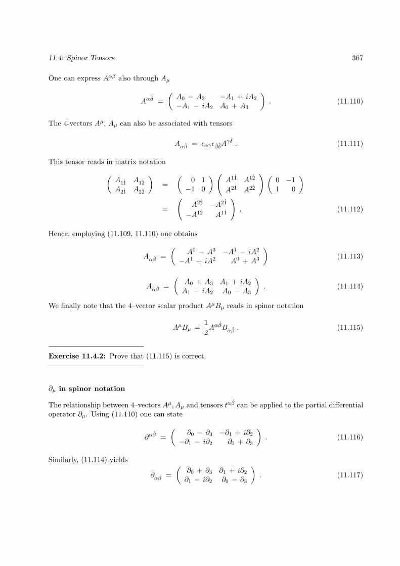
11.4: Spinor Tensors 367
One can express Aαβ also through Aµ
Aαβ =(A0 − A3 −A1 + iA2
−A1 − iA2 A0 + A3
). (11.110)
The 4-vectors Aµ, Aµ can also be associated with tensors
Aαβ = εαγεβδAγδ . (11.111)
This tensor reads in matrix notation(A11 A12
A21 A22
)=
(0 1−1 0
) (A11 A12
A21 A22
) (0 −11 0
)
=
(A22 −A21
−A12 A11
). (11.112)
Hence, employing (11.109, 11.110) one obtains
Aαβ =(
A0 − A3 −A1 − iA2
−A1 + iA2 A0 + A3
)(11.113)
Aαβ =(
A0 + A3 A1 + iA2
A1 − iA2 A0 − A3
). (11.114)
We finally note that the 4–vector scalar product AµBµ reads in spinor notation
AµBµ =12AαβBαβ . (11.115)
Exercise 11.4.2: Prove that (11.115) is correct.
∂µ in spinor notation
The relationship between 4–vectors Aµ, Aµ and tensors tαβ can be applied to the partial differentialoperator ∂µ. Using (11.110) one can state
∂αβ =(
∂0 − ∂3 −∂1 + i∂2
−∂1 − i∂2 ∂0 + ∂3
). (11.116)
Similarly, (11.114) yields
∂αβ =(
∂0 + ∂3 ∂1 + i∂2
∂1 − i∂2 ∂0 − ∂3
). (11.117)
368 Spinor Formulation
σµ in Tensor Notation
We want to develop now the tensor notation for σµ (11.26) and its contravariant analogue σµ
σµ =((
1 00 1
),
(0 11 0
),
(0 −ii 0
),
(1 00 −1
))σµ =
((1 00 1
),
(0 −1−1 0
),
(0 i−i 0
),
(−1 0
0 1
))(11.118)
For this purpose we consider first the transformation behaviour of σµ and σµ. We will obtain thetransformation behaviour of σµ, σµ building on the known transformation behaviour of γµ. This ispossible since γµ can be expressed through σµ, σµ. Comparision of (10.229) and (11.118) yields
γµ =(
0 σµ
σµ 0
). (11.119)
Using (11.15) one can writeσµ = ε (σµ)∗ ε−1 (11.120)
and, hence,
γµ =(
0 σµ
ε (σµ)∗ ε−1 0
). (11.121)
One expects then that the transformation properties of σµ should follow from the transformationproperties established already for γµ [c.f. (10.243)]. Note that (10.243) holds independently of therepresentation chosen, i.e., holds also in the chiral representation.To obtain the transformation properties of σµ we employ then (10.243) in the chiral representationexpressing S(Lηξ) by (11.18) and γµ by (11.121). Equation (10.243) reads then(
a 00 εa∗ε−1
)(0 σµ
ε(σµ)∗ε−1 0
)(a−1 00 εa∗ε−1
)Lνµ =(
0 σν
ε(σν)∗ε−1 0
). (11.122)
The l.h.s. of this equation is(0 aσµε−1(a∗)−1ε
εa∗(σµ)∗ε−1a−1 0
)Lνµ (11.123)
and, hence, one can conclude
aσµε−1(a∗)−1ε Lνµ = σν (11.124)εa∗(σµ)∗ε−1a−1 Lνµ = ε(σν)∗ε−1 . (11.125)
Equation (11.125) is equivalent to
a∗(σµ)∗ε−1a−1ε Lνµ = (σν)∗ (11.126)
which is the complex conjugate of (11.124), i.e., (11.125) is equivalent to (11.124). Hence, (11.124)constitutes the essential transformation property of σµ and will be considered further.

11.4: Spinor Tensors 369
One can rewrite (11.124) using (11.16, 11.2)
ε−1(a∗)−1ε = ε−1e−12~z ∗·~σ ∗ε = e−
12~z ∗·ε−1~σ ∗ε = e
12~z ∗·~σ . (11.127)
Exploiting the hermitian property of ~σ, e.g., (~σ ∗)T = ~σ yields using (11.2)
ε−1(a∗)−1ε = e12~z ∗·(~σ ∗)T =
[e
12~z ∗·~σ ∗
]T= [a∗]T . (11.128)
One can express, therefore, equation (11.124)
a σµ [a∗]T Lνµ = σν . (11.129)
We want to demonstrate now that the expression aσµ[a∗]T is to be interpreted as the transformof σµ under Lorentz transformations. In fact, under rotations the Pauli matrices transform like(j = 1, 2, 3)
σj −→ a(i~ϑ)σj(a(i~ϑ)
)†= a(i~ϑ)σj
(a∗(i~ϑ)
)T. (11.130)
We argue in analogy to the logic applied in going from (11.107) to (11.108) that the same trans-formation behaviour applies then for general Lorentz transformations, i.e., transformations (11.2,11.4) with ~w 6= 0. One can, hence, state that σµ in a new reference frame is
σ′µ = a σµ a† (11.131)
where a is given by (11.2, 11.4). This transformation behaviour, according to (11.102, 11.103)identifies σµ as a tensor of type tαβ . It holds according to (11.118)(
(σµ)11 (σµ)12
(σµ)21 (σµ)22
)=
(1 00 1
)︸ ︷︷ ︸
µ= 0
,
(0 −1−1 0
)︸ ︷︷ ︸
µ= 1
,
(0 i−i 0
)︸ ︷︷ ︸
µ= 2
,
(−1 0
0 1
)︸ ︷︷ ︸
µ= 3
,
(11.132)
and ((σµ)11 (σµ)12
(σµ)21 (σµ)22
)=
(1 00 1
)︸ ︷︷ ︸
µ= 0
,
(0 11 0
)︸ ︷︷ ︸
µ= 1
,
(0 −ii 0
)︸ ︷︷ ︸
µ= 2
,
(1 00 −1
)︸ ︷︷ ︸
µ= 3
,
. (11.133)
Combining (11.129, 11.131) one can express the transformation behaviour of σµ in the succinctform
Lνµ σ′µ = σν . (11.134)

370 Spinor Formulation
Inverting contravariant and covariant indices one can also state
Lνµ σ′µ = σν . (11.135)
This is the property surmised already above [cf. (11.29)]. We can summarize that σµ and σµtransform like a 4–vector, however, the transformation is inverse to that of ordinary 4–vectors.Each of the 4×4 = 16 matrix elements in (11.132) and (11.133) is characterized through a 4-vectorindex µ, µ = 0, 1, 2, 3 as well as through two spinor indices αβ. We want to express now σµ andσµ also with respect to the 4–vector index µ in spinor form employing (11.114). This yields
σαβ =(
σ0 + σ3 σ1 + iσ2
σ1 − iσ2 σ0 − σ3
)= 2
(
1 00 0
) (0 10 0
)(
0 01 0
) (0 00 1
) (11.136)
where on the rhs. the submatrices correspond to tαβ spinors. We can, in fact, state
(σαβ
)γδ=
(
(σ11)11 (σ11)12
(σ11)21 (σ11)22
) ((σ12)11 (σ12)12
(σ12)21 (σ12)22
)(
(σ21)11 (σ21)12
(σ21)21 (σ21)22
) ((σ22)11 (σ22)12
(σ22)21 (σ22)22
) . (11.137)
Equating this with the r.h.s. of (11.136) results in the succinct expression
12
(σαβ
)γδ= δαγδβδ . (11.138)
Note that all elements of σαβ are real and that there are only four non-vanishing elements.In (11.138) the ‘inner’ covariant spinor indices, i.e., α, β, account for the 4–vector index µ, whereasthe ‘outer’ contravariant spinor indices. i.e., γ, δ, account for the elements of the individual Paulimatrices. We will now consider the representation of σµ, σµ in which the contravariant indices aremoved ‘inside’, i.e., account for the 4-vector µ, and the covariant indices are moved outside. Thedesired change of representation(σµ)αβ −→ (σµ)αβ corresponds to a transformation of the basis ofspin states (
fg
)−→
(g−f
)= ε
(fg
)(11.139)
and, hence, corresponds to the transformation((σµ)11 (σµ)12
(σµ)21 (σµ)22
)=(
0 1−1 0
)((σµ)11 (σµ)12
(σµ)21 (σµ)22
)(0 −11 0
)(11.140)
where we employed the expressions (11.12) for ε and ε−1. Using (11.110) to express σαβ in termsof σµ yields together with (5.224)
σαβ =(
σ0 − σ3 σ1 + iσ2
−σ1 − iσ2 σ0 + σ3
)= 2
(
0 00 1
) (0 0−1 0
)(
0 −10 0
) (1 00 1
) (11.141)

11.4: Spinor Tensors 371
and, employing then transformation (11.140) to transform each of the four submatrices, which in(11.137) are in a basis (· · ·)αβ to a basis (· · ·)αβ results in
(σαβ
)γδ
=
(
(σ11)11 (σ11)12
(σ11)21 (σ11)22
) ((σ12)11 (σ12)12
(σ12)21 (σ12)22
)(
(σ21)11 (σ21)12
(σ21)21 (σ21)22
) ((σ22)11 (σ22)12
(σ22)21 (σ22)22
)
= 2
(
1 00 0
) (0 10 0
)(
0 01 0
) (0 00 1
) . (11.142)
This can be expressed12
(σαβ
)γδ
= δαγδβδ . (11.143)
Combined with (11.138) one can conclude that the following property holds
12
(σαβ
)γδ=
12
(σαβ
)γδ
= δαγδβδ . (11.144)
The Dirac Matrices γµ in spinor notation
We want to express now the Dirac matrices γµ in spinor form. For this purpose we start from theexpression (11.121) of γµ. This expression implies that the element of γµ given by ε σµε−1 is in thebasis |αβ whereas the element of γµ given by σµ is in the basis |αβ. Accordingly, we write
γµ =
(0 (σµ)αβ
((σµ)αβ)∗ 0
). (11.145)
Let Aµ be a covariant 4–vector. One can write then the scalar product using (11.115)
γµAµ =
(0 (σµ)αβAµ
((σµ)αβ)∗Aµ 0
)
=
(0 1
2(σγδ)αβAγδ
12((σγδ)αβ)∗Aγδ 0
). (11.146)
Exploiting the property (11.144) results in the simple relationship
γµAµ =
(0 Aαβ
Aαβ 0
). (11.147)

372 Spinor Formulation
11.5 Lorentz Invariant Field Equations in Spinor Form
Dirac Equation
(11.147) allows us to rewrite the Dirac equation in the chiral representation (10.226)
i γµ∂µΨ(xµ) =
(0 i ∂αβ
i ∂αβ 0
)Ψ(xµ) = m Ψ(xµ) . (11.148)
Employing Ψ(xµ) in the form (11.99) yields the Dirac equation in spinor form
i ∂αβ χβ = mφα (11.149)i ∂αβ φ
α = mχβ . (11.150)
The simplicity of this equation is striking.
Chapter 12
Symmetries in Physics: Isospin andthe Eightfold Way
by Melih Sener and Klaus Schulten
Symmetries and their consequences are central to physics. In this chapter we will discuss a particularset of symmetries that have played a seminal role in the development of elementary particle andnuclear physics. These are the isospin symmetry of nuclear interactions and its natural extension,the so-called Eightfold Way.The organization of this chapter is as follows: In the next section we will discuss the relationbetween symmetries of a quantum mechanical system and the degeneracies between its energylevels. We will particularly use the example of spherically symmetric potentials. In the followingsection we will introduce the concept of isospin as an approximate SU(2) symmetry, which identifiesthe proton and the neutron as different states of the same particle. We will also introduce the quarkmodel as a natural framework to represent the observed symmetries. We will apply these conceptsto an analysis of nucleon-nucleon and nucleon-meson scattering. In the final section, we will discussthe SU(3) symmetry of three quark flavors. The algebraic structure and the representations ofSU(3) will be discussed in parallel to SU(2) and particle families will be identified in terms ofrepresentations of the underlying symmetry group.
12.1 Symmetry and Degeneracies
The degeneracies of energy levels of a quantum mechanical system are related to its symmetries.Let us assume a continuous symmetry obeyed by a quantum mechanical system. The action of thesymmetry operations on quantum mechanical states are given by elements of a corresponding Liegroup, i.e.,
O = exp
(∑k
αkSk
). (12.1)
Then the generators, Sk, will commute with the Hamiltonian of the system,
[H,Sk] = 0. (12.2)
373

374 Spinor Formulation
The action of any symmetry generator, Sk, on an energy eigenstate, ψE,λ1,...,λn , leaves the energyof the state invariant
H exp(iαkSk) ψE,λ1,...,λn = E exp(iαkSk) ψE,λ1,...,λn . (12.3)
If the newly obtained state is linearly independent of the original one, this implies a degeneracy inthe spectrum. We will investigate this shortly in more detail in the case of systems with sphericalsymmetry, where the symmetry generators, Sk, can be identified with the angular momentumoperators, Jk, as studied in chapter 7.Lie groups play an essential role in the discussion of mass degeneracies in particle physics. In orderto illustrate this, we first consider a particular example of the implications of symmetry, namelymotion in a spherically symmetric potential described by the group SO(3) (or its double coveringSU(2) as discussed in section 5.12).In chapter 7 the dynamics of a particle moving in three dimensions under the influence of a spher-ically symmetric potential, V (r), has been discussed. The spherical symmetry implies the commu-tation of the Hamiltonian with angular momentum operators (7.8)
[H, Jk] = 0 , k = 1, 2, 3 . (12.4)
The stationary Schrodinger equation, (7.18), can then be reduced to a one-dimensional radialequation, (7.24), which yields a set of eigenstates of the form
ψE,`,m(~r) = vE,`,m(r)Y`m(θ, φ), (12.5)
with m = −l, . · · · , l and the corresponding energy levels are independent of m. Therefore, eachenergy level is (2l + 1)-fold degenerate. This degeneracy follows from the fact that any rotation,as represented by an element of SO(3), (7.39), generates a state which has the same energy as theoriginal one.
Presence of additional symmetries may further increase the degeneracy of the system. As anexample of this we will consider the Coulomb problem with the Hamiltonian
H =~p2
2m− k
r. (12.6)
From elementary quantum mechanics we know the spectrum of the hydrogen atom. The energylevels are
En = − mk2
2~2n2, (12.7)
where the orbital angular momentum, l, is allowed to take values in 0, . . . , n− 1. The energy levelsare totally independent of l. For example, the states 3s, 3p and 3d all have the same energy. Wewant to understand this extra degeneracy in terms of the extra symmetry of the hydrogen atomgiven by an additional set of symmetry generators introduced below.Classically, the additional symmetry generators of the Coulomb problem are the three componentsof the so-called eccentricity vector discovered by Hamilton
~ε =1m~p× ~J − k~r
r. (12.8)
11.5: Lorentz Invariant Field Equations 375
The vector ~ε points along the symmetry axis of the elliptical orbit and its length equals the eccen-tricity of the orbit. The vector in (12.8) is not a hermitian operator. The corresponding quantummechanical hermitian operator can be defined by
ε1 =1
2m(p2J3 − p3J2 + J3p2 − J2p3)− kx1
r, (12.9)
ε1 =1
2m(J3p2 − J2p3 + i~p1)− kx1
r, (12.10)
ε2 =1
2m(J1p3 − J3p1 + i~p2)− kx2
r, (12.11)
ε3 =1
2m(J2p1 − J1p2 + i~p3)− kx3
r, (12.12)
(12.13)
It can be verified explicitly that its components commute with the Hamiltonian.In order to understand the aforementioned extra degeneracy, we will compute the hydrogen spec-trum using the additional symmetry. For this purpose we first note that
~J · ~ε = 0. (12.14)
This follows from ~a · (~a×~b) = (~a×~b) · ~a = 0, which is valid even when ~a and ~b do not commute.We will also need the following identity [4]
~ε2 =2Hm
(~J2 + ~2
)+ k2, (12.15)
which can be proved after very considerable algebra.In the following we consider the bound states, which have a negative energy E. Therefore, in thesubspace of the Hilbert space corresponding to a certain energy we can replace H by E. Now wescale the eccentricity vector as follows
~K =√− m
2E~ε. (12.16)
Through some algebra [4] the following commutation relations can be verified
[Ki, Jj ] = i~εijkKk, (12.17)[Ki,Kj ] = i~εijkJk, (12.18)
which complement the familiar angular momentum algebra of section 5.3.We introduce the following new operators
~A =12
( ~J + ~K), (12.19)
~B =12
( ~J − ~K), (12.20)
which can be shown to satisfy
[Ai, Aj ] = i~εijkAk, (12.21)

376 Spinor Formulation
[Bi, Bj ] = i~εijkBk, (12.22)[Ai, Bj ] = 0, (12.23)[~A,H
]= 0, (12.24)[
~B,H]
= 0. (12.25)
So far we have shown that the symmetry generators form an algebra, which is identical to the thedirect sum of the Lie algebra of of two SO(3) (or SU(2)) algebras. By comparing to the rotationalgebra introduced in chapter 5, we can read off the eigenvalues of ~A2 and ~B2 from (12.21) and(12.22):
~A2 = a(a+ 1)~2 , a = 0,12, 1, . . . , (12.26)
~B2 = b(b+ 1)~2 , b = 0,12, 1, . . . . (12.27)
Following (12.14) we note that~A2 − ~B2 = ~J · ~ε = 0. (12.28)
This implies that a = b. In order to arrive at the spectrum a final bit algebra is needed
~A2 + ~B2 = ~J2 + ~K2 (12.29)
= ~J2 − m
2E~ε2 (12.30)
= −mk2
4E− 1
2~
2, (12.31)
where we have used (12.15). Using this equation the energy eigenvalues can be written in termsof the eigenvalues of ~A2 and ~B2 operators. Noticing that ~A2 and ~B2 have the same eigenvaluesbecause of (12.28), the energy eigenvalues are found to be
E = − mk2
2~2(2a+ 1)2, a = 0,
12, 1, . . . . (12.32)
A comparison with (12.7) tells us that (2a+ 1) = n. Furthermore the bound on the orbital angularmomentum, l, can be seen to follow from the triangle inequality as applied to ~J = ~A+ ~B, namelythat ∣∣∣ ~J∣∣∣ >
∣∣∣ ~A∣∣∣− ∣∣∣ ~B∣∣∣ = 0 (12.33)∣∣∣ ~J∣∣∣ <∣∣∣ ~A∣∣∣+
∣∣∣ ~B∣∣∣ = 2∣∣∣ ~A∣∣∣ (12.34)
It follows that l has to have values in 0 = |a− b|, 1, . . . , a+ b = n− 1. This illustrates the effectof additional symmetries to the degeneracy structure of a quantum mechanical system.
In contrast to the discussion above about extra symmetries, a lack of symmetry implies a lack ofdegeneracy in the energy levels of a quantum mechanical system. The most extreme case of this isthe quantum analogue of a classically chaotic system. Chaos is described classically as exponential

11.5: Lorentz Invariant Field Equations 377
sensitivity to initial conditions, in the sense that nearby trajectories in the phase space diverge fromeach other over time. However, another manifestation of chaos is the lack of independent operatorscommuting with the Hamiltonian.A typical example of this so called quantum chaos is the quantum billiard problem, which is aparticle in box problem in two dimensions with a boundary which can be chosen arbitrarily. If thechosen boundary is ‘irregular’ in a suitably defined sense, the classical trajectories will diverge fromeach other after successive bounces from the boundary. For a more detailed discussion of quantumchaos in billiard systems we refer the reader to [7] and the references therein.In the case of billiards and other examples of quantum chaos one common observation is the almostnonexistence of degeneracies and the fact that the energy levels are more evenly spaced. This isknown as level repulsion.
In the next section we will proceed with the discussion of a symmetry, which was discovered byobserving degeneracies in the particle spectrum.
12.2 Isospin and the SU(2) flavor symmetry
The concept of isospin goes back to Heisenberg, who, after the discovery of the neutron in 1932,suggested that the proton and the neutron can be regarded as two states of a single particle. Thiswas motivated by the observation that their masses are approximately equal: mp = 938.28MeV/c2,mp = 939.57MeV/c2. Following the mass-energy equivalence of special relativity
E = mc2, (12.35)
this mass equivalence can be viewed as an energy degeneracy of the underlying interactions.This (approximate) degeneracy led into the idea of the existence of an (approximate) symmetryobeyed by the underlying nuclear interactions, namely, that the proton and the neutron behaveidentically under the so-called strong interactions and that their difference is solely in their chargecontent. (Strong interactions bind the atomic nucleus together.)If the proton and the neutron are to be viewed as two linearly independent states of the sameparticle, it is natural to represent them in terms of a two component vector, analogous to thespin-up and spin-down states of a spin-1
2 system
p =(
10
), n =
(01
). (12.36)
In analogy to the concept of spin regarding the rotations in 3-space as discussed in chapter 5, theisospin symmetry is also governed by an SU(2) group ‘rotating’ components in (12.36) into eachother in abstract isospin space. This enables us to utilize what we already know about the SU(2)symmetry group from the study of angular momentum. For example, we will be able to use thefamiliar Clebsch-Gordan coefficients to combine the isospin of two particles the same way we addedspin in chapter 6.It is important to place the isospin concept in its proper historical context. Originally it wasbelieved that isospin was an exact symmetry of strong interactions and that it was violated byelectromagnetic and weak interactions. (Weak interactions are responsible, for example, for the
378 Spinor Formulation
beta decay). The mass difference between the neutron and the proton could then be attributed tothe charge content of the latter. If the mass difference (or the energy difference) were to be to bepurely electrostatic in nature, the proton had to be heavier. However, the proton is the lighter ofthe two. If it were otherwise the proton would be unstable by decaying into the neutron, spellingdisaster for the stability of matter.Isospin symmetry is not an exact symmetry of strong interactions, albeit it is a good approximateone. Therefore it remains a useful concept. Further than that, as we shall see below, it can be seenas part of a larger (and more approximate) symmetry which is of great utility to classify observedparticle families.
We can describe isospin multiplets the same way we have described the angular momentum and spinmultiplets. Denoting the total isospin, I, and its third component, I3, as good quantum numbers,we can re-write (12.36) as a multiplet with I = 1
2
p =∣∣∣∣I =
12, I3 =
12
⟩, n =
∣∣∣∣I =12, I3 = −1
2
⟩. (12.37)
As an example of a multiplet with I = 1 we have the three pions or π-mesons
π+ = |1, 1〉 , π0 = |1, 0〉 , π− = |1,−1〉 , (12.38)
which have all nearly identical masses. (mπ± = 139.6MeV/c2, mπ0 = 135.0MeV/c2). Shortly wewill see how to describe both the pion and nucleon states as composites of more fundamental I = 1
2states.In the framework of the quark of model, the fundamental representation of the isospin symmetrycorresponds to the doublet that contains the so-called up and down quarks
u =∣∣∣∣12 , 1
2
⟩, d =
∣∣∣∣12 ,−12
⟩. (12.39)
All other isomultiplets, including the proton and the neutron, are made up of these two quarks.They can be constructed with the same rules that have been used for angular momentum additionin chapter 6. For example, the three pions in (12.38) are ud, uu and du states, respectively. Theyform an isotriplet:
π+ = |1, 1〉 =∣∣∣∣12 , 1
2
⟩1
∣∣∣∣12 , 12
⟩2
, (12.40)
π0 = |1, 0〉 =1√2
(∣∣∣∣12 , 12
⟩1
∣∣∣∣12 ,−12
⟩2
+∣∣∣∣12 , 1
2
⟩1
∣∣∣∣12 ,−12
⟩2
), (12.41)
π− = |1,−1〉 =∣∣∣∣12 ,−1
2
⟩1
∣∣∣∣12 ,−12
⟩2
. (12.42)
(12.43)
Similarly, the proton and the neutron can be written as totally symmetric uud and udd states. Fora precise description of the two nucleons as composite states, including the spin and color quantumnumbers of their constituent quarks, we refer the reader to [1], sec. 2.11.

11.5: Lorentz Invariant Field Equations 379
The mass of the up and down quarks are not identical but they are both of the order of a fewMeV/c2’s which is minuscule compared to the typical energy scale of hadrons (i.e. strongly inter-acting particles) which is about a GeV/c2. This is why isospin is such a good symmetry and whyisomultiplets have nearly identical masses.As it later turned out, the up and down quarks are not the only quark ‘species’ - or flavors asthey are commonly called. In the late 1940’s and early 1950’s, a number strange particles havebeen found which presumably contained a third quark species: the strange quark. It shall be notedhere that the quark model was not invented until 1960’s, but at the time the empirical conceptslike isospin and strangeness quantum numbers were in use. The value of the strangeness quantumnumber is taken, by accidental convention, to be −1 for the strange quark. The up and downquarks have strangeness zero. All other composite states have their strangeness given by the sumof the strangeness content of their constituents.Before proceeding further, we shall setup some terminology: baryons are qqq states, such as protonand the neutron, whereas mesons are qq states, the pions being examples thereof. By conventionbaryons have baryon number 1, and quarks have baryon number 1
3 . All antiparticles have theirquantum numbers reversed. Naturally, mesons have baryon number 0. The names, baryon andmeson, originally refer to the relative weight of particles, baryons generally are heavy, mesons haveintermediate mass ranges, where leptons (electron, muon, the neutrinos etc.) are light. If takenliterally, this remains only an inaccurate naming convention today, as some mesons discovered laterare heavier than some baryons and so on.The relation between electric charge and isospin are given by the Gell-Mann–Nishijima relationwhich was first derived empirically
Q = I3 +12
(B + S), (12.44)
where B is the baryon number and S is the strangeness. In the next section we will be able toview the Gell-Mann–Nishijima relation in the light of the representation theory for the flavor SU(3)symmetry.
Now let us consider another example of combining the isospins of two particles. The reader mayknow that the deuteron, a hydrogen isotope, consists of a proton and a neutron. Therefore it hasto have isospin, I3 = 0. We will now try to describe its wave function in terms of its constituentnucleons. Following (12.37) and in analogy to (12.43), this will be mathematically identical toadding two spins. The possibilities are that of an isosinglet
|0, 0〉 =1√2
(|p > |n > −|n > |p >) (12.45)
and that of an isotriplet
|1, 1〉 = |p > |p >, (12.46)
|1, 0〉 =1√2
(|p > |n > +|n > |p >), (12.47)
|1,−1〉 = |n > |n > . (12.48)
Is the deuteron an isosinglet state or an isotriplet? If it were an isotriplet (|1, 0〉) we should haveseen nn and pp bound states of comparable energy in nature (because of isospin symmetry), butsuch states do not exist. Therefore the deuteron has to be an isosinglet state (|0, 0〉).

380 Spinor Formulation
As an exercise on the implications of isospin symmetry we will consider nucleon-nucleon scattering.We will eventually be able to compute ratios of scattering cross-sections between different processes.For example, consider
(I) p+ p→ d+ π+
(II) p+ n→ d+ π0 (12.49)
The only assumption that we put in will be that the interaction is of the form V = α I(1) · I(2). Thedot product here refers to the abstract isospin space. The cross-section, σ, is proportional to |M|2,where M is the scattering amplitude given by
M = 〈 final | α I(1) · I(2) | initial 〉 . (12.50)
The initial and final states can be denoted in more detail as
| initial 〉 =∣∣∣ I(i), I
(i)3 , γ(i)
⟩, (12.51)
| final 〉 =∣∣∣ I(f), I
(f)3 , γ(f)
⟩, (12.52)
where γ(i) and γ(f) denote degrees of freedom other than isospin, such as the spatial dependenceof the wave function and spin.
Exercise. Consider the generalization of tensor operators discussed in section 6.7 to the case ofisospin. Show that I(1)·I(2) is an ‘isotensor’ of rank zero. Refer to exercise 6.7.5 for the spin-analogueof the same problem.
Exercise. Show that the expectation of I(1) · I(2) is 14 in an isotriplet state and −3
4 in an isosingletstate.
Using (12.38) and the fact that the deuteron is an isosinglet we know that the isospins of the finalstates in (I) and (II) are |1, 1〉 and |1, 0〉, respectively. According to (12.45) and (12.48) the initialstates in (I) and (II) have isospin values |1, 1〉 and (1/
√2)(|1, 0〉+ |0, 0〉). We will now employ the
(isospin analogue) of the Wigner-Eckart theorem (6.259) discussed in detail in sections 6.7 and 6.8to compute the ratio of the scattering amplitudes MI and MII. For completeness let us start byrestating the Wigner-Eckart theorem (6.259) in the present context:
〈I(f)I(f)3 , γ(f)|T00|I(i)I
(i)3 , γ(i)〉 = (12.53)
(I(f)I(f)3 |00I(i)I
(i)3 ) (−1)I
(f)−I(i) 1√2I(i)+1
〈I(f), γ(f)||T0||I(i), γ(i)〉. (12.54)
Here T00 ≡ V = α I(1) · I(2), which is an isoscalar, as discussed in the exercise above.(I(f)I
(f)3 |00I(i)I
(i)3 ) is a Clebsch-Gordon coefficient and 〈I(f), γ(f)||T0||I(i), γ(i)〉 is a reduced ma-
trix element defined in the same sense as in section 6.8.Now let us re-write more carefully the scattering amplitudes for the two processes in the light ofwhat we have just learned
MI =⟨I(f) = 1, I(f)
3 = 1, γ(f)∣∣∣T00
∣∣∣ I(i) = 1, I(i)3 = 1, γ(i)
⟩(12.55)

11.5: Lorentz Invariant Field Equations 381
= (11|0011)1√3〈I(f) = 1, γ(f) ||T00|| I(i) = 1, γ(i)〉 (12.56)
MII =1√2
⟨I(f) = 1, I(f)
3 = 0, γ(f)∣∣∣T00
∣∣∣ I(i) = 1, I(i)3 = 0, γ(i)
⟩(12.57)
+1√2
⟨I(f) = 1, I(f)
3 = 0, γ(f)∣∣∣T00
∣∣∣ I(i) = 0, I(i)3 = 0, γ(i)
⟩(12.58)
= (10|0010)1√3〈I(f) = 1, γ(f) ||T00|| I(i) = 1, γ(i)〉 (12.59)
+0. (12.60)(12.61)
Note that the second term inMII vanishes due to the isospin conservation, which is also manifestedby a vanishing Clebsch-Gordon prefactor. The relevant Clebsch-Gordon coefficients are easilyevaluated:
(11|0011) = (10|0010) = 1. (12.62)
We can now write the ratio of the scattering amplitudes:
MI
MII=
1(1/√
2), (12.63)
where common dynamical factors (which would not be as easy to compute) have dropped outthanks to the Wigner-Eckart theorem. It follows
σI
σII= 2, (12.64)
which is in approximate agreement with the observed ratio. [2]
As a further example, we will consider pion-nucleon scattering. We want to compute the ratio oftotal cross-sections assuming a similar interaction as in the previous example
σ(π+ + p → anything )σ(π− + p → anything )
.
The possibilities are
(a) π+ + p → π+ + p ,(b) π− + p → π− + p ,(c) π− + p → π0 + n .
(12.65)
There are more exotic possibilities, involving, for example, particles with strangeness, but these arenot dominant at relatively low energies.Once again we need the isospins for the initial and final states, which are obtained by a standardClebsch-Gordan expansion
π+ + p : |1, 1〉∣∣1
2 ,12
⟩=∣∣3
2 ,32
⟩,
π− + p : |1,−1〉∣∣1
2 ,12
⟩= 1√
3
∣∣32 ,−
12
⟩−√
23
∣∣12 ,−
12
⟩,
π0 + n : |1, 0〉∣∣1
2 ,−12
⟩=√
23
∣∣32 ,−
12
⟩+ 1√
3
∣∣12 ,−
12
⟩.
(12.66)

382 Spinor Formulation
As in the example of nucleon-meson scattering we define the relevant matrix elements
M 32
=⟨
32 ,m
∣∣ V ∣∣ 32 ,m
⟩,
M 12
=⟨
12 ,m
∣∣ V ∣∣ 12 ,m
⟩,
(12.67)
which are independent of m. A computation similar to the previous example of nucleon-nucleonscattering yields (apart from common prefactors) the following amplitudes for the reactions in(12.65)
Ma =M 32
Mb = 13M 3
2+ 2
3M 12
Mc =√
23 M 3
2−√
23 M 1
2
(12.68)
Guided by empirical data we will further assume that M 32>>M 1
2, which leads to the following
ratios for the cross-sections
σa : σb : σc = 9 : 1 : 2. (12.69)
As the total cross-section is the sum of individual processes we obtain
σ(π+ + p )σ(π− + p )
=σa
σb + σc= 3 (12.70)
again in approximate agreement with the observed value. [2]
12.3 The Eightfold Way and the flavor SU(3) symmetry
The discovery of the concept of strangeness, mentioned in the previous section, was motivatedby the existence of particles that are produced strongly but decay only weakly. For instance,K+, which can be produced by π− + p → K+ + Σ−, has a lifetime which is comparable to thatof π+ albeit being more than three times heavier. Hence Gell-Mann and independently Nishijimapostulated the existence of a separate quantum number, S, called strangeness, such that S(K+) = 1,S(Σ−) = −1 and S(π) = S(N) = 0, etc. It was assumed that strong interactions conserved S (atleast approximately), while weak interactions did not. Hence the strangeness changing strongdecays of K+ (or Σ−) were forbidden, giving it a higher than usual lifetime.The classification of the newly found particles as members of some higher multiplet structurewas less obvious then the case of isospin, however. Strange partners of the familiar nucleons, forexample, are up to 40% heavier, making an identification of the underlying symmetry and themultiplet structure less straightforward.In the light of the quark model, it appears an obvious generalization to add another component foran extra quark to the isospin vector space
u =
100
, d =
010
, s =
001
. (12.71)

11.5: Lorentz Invariant Field Equations 383
In this case the transformations that ‘rotate’ the components of (12.71) into each other, whilepreserving the norm, have to be elements of the group SU(3) (which we will investigate closelyvery soon). However, history followed the reverse of this path. First particle multiplets wereidentified as representations of the SU(3) group, the same way nucleons and pions were identifiedas representations of the isospin SU(2) symmetry. Then came the question of what the fundamentalrepresentation, as in (12.71), should correspond to, giving rise to the quark model. As quarks werenever directly observed, for a period they were considered as useful bookkeeping devices withoutphysical content.In this perspective the flavor SU(3) symmetry may appear to be mainly of historical interest.However SU(3) symmetry appears in another and much more fundamental context in strong in-teraction physics. The quarks posses another quantum number, called color, which again formrepresentations of an SU(3) group. This is believed to be an exact symmetry of strong interac-tions, in fact modern theory of strong interactions is a ‘gauge theory’ of this color group, calledquantum chromodynamics. (The reader is referred to section 8.3 for a brief discussion of gaugetransformations). Flavor SU(Nf ) symmetry on the other hand, where Nf is the number quarkflavors, becomes increasingly inaccurate for Nf > 3. The reason is that the other known quarks,namely charm, bottom (beauty) and top (truth) are significantly heavier than the hadronic energyscale. (The ‘bare’ mass of the charm quark is already heavier than the two nucleons, which set thehadronic energy scale. The bottom and top are even heavier. [2] )
Before discussing the significance and the physical implications of the quark model, we will establishsome mathematical preliminaries about the group SU(3). In many respects it will resemble themore familiar group SU(2) discussed in some detail in chapter 5, but there are a number of subtledifferences. The reader shall note that most of what is being said trivially generalizes to otherunitary groups, SU(N), but we will stick to N = 3 in the following. The reader is also invited torevisit section 5.1 whenever necessary, in reference to Lie groups, Lie algebras and related concepts.
Given a complex vector, ak, of three dimensions, we want to find those transformations
ak → Uklal (12.72)
that preserve the norm,∑
k a∗kak, of a. It is seen that such a matrix U has to satisfy the following
unitary relation
U † = U−1. (12.73)
To verify that all such matrices form a group, we observe that
(UV )† = V †U † = V −1U−1 = (UV )−1, (12.74)
for any two unitary matrices U and V . This group of 3 × 3 unitary matrices is denoted by U(3).The unitarity relation imposes 9 constraints on the total of 18 real degrees of freedom of a 3 × 3complex matrix. Hence the group U(3) has 9 dimensions. Multiplying U by a phase, eiφ, still leavesthe norm invariant. Therefore U(3) can be decomposed into a direct product U(1)× SU(3) whereSU(3) consists of 3× 3 unitary matrices of unit determinant. Because of this additional constraintSU(3) has 8 dimensions. Since arbitrary phase factors are of no physical interest, it is the group

384 Spinor Formulation
SU(3) and not U(3) that is of main interest. The reader is invited to compare the structure ofSU(3) to that of SU(2) discussed in section 5.7.
As discussed in section 5.1, any unitary matrix, U , can be written in the form
U = eiH (12.75)
where H is a hermitian matrix. Therefore we will express elements of SU(3) as
U = ei∑k αkλk (12.76)
where λk are 8 linearly independent matrices forming the basis of the Lie algebra of SU(3). (Weshall at times refer to the Lie algebra with the name of the group, the meaning being apparent fromthe context.) The unit determinant condition requires that all λk are traceless, since det(eA) = etrA.An explicit basis is constructed in analogy to the Pauli algebra of spin operators
λ1 =
0 1 01 0 00 0 0
, λ2 =
0 −i 0i 0 00 0 0
, λ3 =
1 0 00 −1 00 0 0
,
λ4 =
0 0 10 0 01 0 0
, λ5 =
0 0 −i0 0 0i 0 0
,
λ6 =
0 0 00 0 10 1 0
, λ7 =
0 0 00 0 −i0 i 0
,
λ8 = 1√3
1 0 00 1 00 0 −2
.
(12.77)
The generators, λk, obey the following relation
tr(λjλk) = 2δjk, (12.78)
which can be verified explicitly as matrix identities.The Lie algebra structure is given by the commutators of λk
[λj , λk] = 2ifjklλl, (12.79)
where fjkl are the antisymmetric structure constants similar to the εjkl of SU(2) given in (5.32).We can also introduce the constants, δjkl, via the anticommutator relation
[λj , λk]+ =43δjk + 2δjklλl, (12.80)
This is the fundamental or defining representation of SU(3). As in the case of SU(2) higherdimensional representations obeying the same structure can be found. The fundamental relationto be preserved is (12.79), regardless of the dimension of the representation.

11.5: Lorentz Invariant Field Equations 385
As it turns out the set of generators in (12.77) is not the most useful basis in the study of SU(3).In the case of SU(2) the identification of ‘ladder’ operators J+, J− proved useful, which satisfiedan ‘eigenvalue equation’
[J0, J±] = ±~J±. (12.81)
In chapter 5, these relations have been used to construct the angular momentum spectrum as wellas the function space representation of the rotation algebra, namely spherical harmonics. Thegenerators of SU(3) can be arranged into a very similar form to that of SU(2). We first introducethe F-spin operators
Fi =12λi. (12.82)
With another change of basis we arrive at the ‘standard’ form of the generators of the Lie algebraof SU(3)
T± = F1 ± iF2, (12.83)T0 = F3, (12.84)V± = F4 ± iF5, (12.85)U± = F6 ± iF7, (12.86)
Y =2√3F8. (12.87)
Exercise. Using the convention in (12.71) show that T0 is the isospin operator, I3.
Exercise. Derive the Gell-Mann–Nishijima relation (12.44), starting with the observation thatY = B+S. (Recall that the strange quark has S = −1 by convention). Y is called the hypercharge.
In the basis (12.87) the commutation relations between the generators can be expressed in a succinctmanner. First, we have
[Y, T0] = 0, (12.88)
which defines (not uniquely) a maximal set of mutually commuting operators Y, T0 and
[Y, T±] = 0, (12.89)[Y, U±] = ±U±, (12.90)[Y, V±] = ±V±, (12.91)
[T0, T±] = ±T±, (12.92)
[T0, U±] = ∓12U±, (12.93)
[T0, V±] = ±12V±, (12.94)

386 Spinor Formulation
which relate the remaining generators T±, V±, U± to this maximal set by ‘eigenvalue equations’and
[T+, T−] = 2T0, (12.95)
[U+, U−] =32Y − T0 = 2U0, (12.96)
[V+, V−] =32Y + T0 = 2V0, (12.97)
which relate commutators of generators with opposite eigenvalues to the maximal set Y, T0. Notethat, U0 and V0 are linear combinations of T0 and Y . Finally, we have
[T+, V−] = −U−, (12.98)[T+, U+] = V+, (12.99)[U+, V−] = T−, (12.100)[T+, V+] = 0, (12.101)[T+, U−] = 0, (12.102)[U+, V+] = 0. (12.103)
Any remaining commutators follow from hermiticity.The same way the angular momentum ladder operators have been used to construct the represen-tations of SU(2), we will use these commutation relations to construct representations of SU(3).In the case of SU(2) the representations lay on a line on the J0 axis. However, since there are twomutually commuting generators in SU(3) as given in (12.88), the representations will now lie in aT0 − Y -plane. The maximum number of mutually commuting generators of a Lie algebra is calledits rank. Thus, SU(2) has rank 1, while SU(3) has rank 2.When the basis of a Lie algebra is expressed in such a way to satisfy the form of the eigenvaluerelations as given above, it is said to be in Cartan-Weyl form. This form is essential for easy labelingof the representations of the group, as the relation between the states in a given representationcan be conveniently expressed in terms of ladder operators. A formal definition and a detaileddiscussion of the Cartan-Weyl form is beyond the scope of this chapter. The interested reader isinstead referred to a very readable account given in chapter 12 of [4].
Another important property of SU(2) is the existence of an operator (namely the total angularmomentum, J2) which commutes with all of the generators. An operator which commutes with allgenerators of a Lie group is called a Casimir operator. As in the case of J2 and SU(2), Casimiroperators can be used to label irreducible representations of the Lie algebra, similar to the way itwas done in section 5.5. We can construct two such independent Casimir operators for the groupSU(3).
C1 =∑k
λ2k = −2i
3
∑jkl
fjklλjλkλl, (12.104)
C2 =∑jkl
djklλjλkλl (12.105)
In general the number of independent Casimir operators of a Lie group is equal to its rank.

11.5: Lorentz Invariant Field Equations 387
The utility of Casimir operators arises from the fact that all states in a given representation assumethe same value for a Casimir operator. This is because the states in a given representation areconnected by the action of the generators of the Lie algebra and such generators commute withthe Casimir operators. This property can be used to label representations in terms of the valuesof the Casimir operators. For example, it was shown in section 5.5 how to label the irreduciblerepresentations of the angular momentum algebra SU(2) in terms of the value of the total angularmomentum.
Now we will construct explicit representations of SU(3). Because of (12.88) we can label states bythe eigenvalues of T0 and Y operators, |t3, y〉:
T0 |t3, y〉 = t3 |t3, y〉 , (12.106)Y |t3, y〉 = y |t3, y〉 . (12.107)
From the commutation relations we have presented above (the Cartan-Weyl form) we can writedown the effect of various generators on the state |t3, y〉. For example, we have
U0 |t3, y〉 = (34y − 1
2t3) |t3, y〉 , (12.108)
V0 |t3, y〉 = (34y +
12t3) |t3, y〉 . (12.109)
The same way that J± |m〉 is proportional to |m± 1〉 in the case of the angular momentum algebra,we have
T± |t3, y〉 = α
∣∣∣∣t3 ± 12, y
⟩, (12.110)
U± |t3, y〉 = β
∣∣∣∣t3 ± 12, y ± 1
⟩, (12.111)
V± |t3, y〉 = γ
∣∣∣∣t3 ∓ 12, y ± 1
⟩. (12.112)
The effect of these operators to the states in the y − t3 plane have been outlined in Fig. (12.1).The representations of SU(3) are constructed analogous to those of SU(2) by identifying the ‘bound-ary’ states annihilated by raising (or lowering) operators. All other states of the representationare then constructed by successive application of ladder operators T±, U±, V±. The representationsfor hexagons with sides of length p and q in the T0 − Y -plane. Such a representation is labeled asD(p, q) and it has a dimensionality of 1
2(p + 1)(q + 1)(p + q + 2). Figure (12.2) shows the repre-sentation D(2, 1) as an example. The details of this procedure is beyond the scope of this chapter.The interested reader is referred to [4], especially chapters 7 and 8.As another example for the representations of SU(3), the pion family forms part of an octet corre-sponding to the D(1, 1) representation. The representations D(1, 0) and D(0, 1) correspond to thetriplets of quarks and antiquarks, respectively. (See Fig. (12.3).) All other representations can beconstructed by combining these two conjugate representations. For example the pion octet (or anyother meson octet) is therefore realized as states of a quark - antiquark pair. A notation suggestiveof the dimensionality of the representation can be used to identify representations. For example,

388 Spinor Formulation
Figure 12.1: The effect of SU(3) ladder operators on the y − t3 plane.
! #"%$&
Figure 12.2: D(2, 1) representation of SU(3). The states in the inner triangle are doubly degenerate.

11.5: Lorentz Invariant Field Equations 389
D(1, 0) and D(0, 1) are denoted by [3] and [3], respectively. The octet D(1, 1) is written as [8] etc.This way the quark-antiquark states can be represented as follows
[3]⊗ [3] = [8]⊕ [1] (12.113)
The additional singlet state corresponds to the η′ meson. This expansion can be compared, forexample, to the case of adding two spin triplet states, in the case of SU(2), where we would write
[3]⊗ [3] = [1]⊕ [3]⊕ [5]. (12.114)
Figure 12.3: D(1, 0) or the fundamental representation of flavor SU(3) symmetry.
The three quarks in the fundamental representation can now be written as
u =∣∣∣∣12 , 1
3
⟩, (12.115)
d =∣∣∣∣−1
2,13
⟩, (12.116)
s =∣∣∣∣0,−2
3
⟩. (12.117)
The Gell-Mann–Nishijima relation can then be succinctly expressed as
Q =12y + t3, (12.118)
390 Spinor Formulation
from which the quark charges follow
Qu =23, (12.119)
Qd = −13, (12.120)
Qs = −13. (12.121)
S +S - S 0
L 0
X - X 0
Figure 12.4: The baryon octet as a D(1, 1) representation of SU(3).
References
[1] Quarks and leptons: an introductory course in particle physics, F. Halzen, A. D. Martin, 1984,Wiley.
[2] Introduction to elementary particles, D. Griffiths, 1987, Wiley.
[3] Microscopic theory of the nucleus, J. M. Eisenberg, W. Greiner, 1972, North holland.
[4] Quantum mechanics: symmetries, W. Greiner, B. Muller, 1989, Springer-Verlag
[5] Principles of symmetry, dynamics, and spectroscopy, W. G. Harter, 1993, Wiley.
[6] Gauge theory of elementary particle physics, T.-P. Cheng, L.-F. Li, 1984, Oxford.
[7] Expansion method for stationary states of quantum billiards, D. L. Kaufman, I. Kosztin, K.Schulten, Am. J. Phys. 67 (2), p. 133, (1999).