a kinetic transport and reaction model and simulator for ...gobbert/papers/gobbertcalejcp2006.pdfa...

Journal of Computational Physics 213 (2006) 591–612

www.elsevier.com/locate/jcp

A kinetic transport and reaction model and simulatorfor rarefied gas flow in the transition regime

Matthias K. Gobbert a,*, Timothy S. Cale b

a Department of Mathematics and Statistics, University of Maryland, Baltimore County, 1000 Hilltop Circle, Baltimore, MD 21250, USAb Focus Center – New York, Rensselaer: Interconnections for Hyperintegration, Isermann Department of Chemical and

Biological Engineering, Rensselaer Polytechnic Institute, CII 6015, 110 8th Street, Troy, NY 12180-3590, USA

Received 17 June 2005; received in revised form 24 August 2005; accepted 25 August 2005Available online 14 October 2005

Abstract

We present a model for rarefied gas flows that are characterized by reactive species as minor constituents in a dominantinert carrier species. The kinetic transport and reaction model consists of a system of transient linear Boltzmann equationsfor the reactive species in the flow. This model applies to a wide range of transport regimes, including the transition regimein which both transport and collisions between molecules must be taken into account, characterized by Knudsen numberson the order of unity. A numerical simulator based on a spectral Galerkin method in velocity space approximates eachlinear Boltzmann equation by a system of transient conservation laws in space and time with diagonal coefficient matrices,which are solved using the discontinuous Galerkin method. This deterministic solver gives direct access to the kinetic den-sity that is the solution to the Boltzmann equation, as a function of position, velocity, and time. It is valuable to have directaccess to the velocity dependence in order to analyze the underlying kinetic causes of macroscopic observeables. Usingchemical vapor deposition as an important application example, the influence of process parameters is studied in two-dimensional reference studies and transient studies for a three-dimensional domain that represents structures seen duringintegrated circuit fabrication.� 2005 Elsevier Inc. All rights reserved.

Keywords: Rarefied gas flow; Boltzmann transport equation; Spectral Galerkin method; Discontinuous Galerkin method; Chemical vapordeposition

1. Introduction

Many important manufacturing processes for integrated circuits involve the flow of gaseous reactants atpressures that range from very low to atmospheric [18]. Correspondingly, the mean free path k (the averagedistance that a molecule travels before colliding with another molecule) ranges from less than 0.1 lm to over100 lm. The typical size of the electronic components (called �features� during integrated circuit processing) is

0021-9991/$ - see front matter � 2005 Elsevier Inc. All rights reserved.

doi:10.1016/j.jcp.2005.08.026

* Corresponding author. Tel.: +1 410 455 2404; fax: +1 410 455 1066.E-mail addresses: [email protected] (M.K. Gobbert), [email protected] (T.S. Cale).

mailto:[email protected]

mailto:[email protected]

592 M.K. Gobbert, T.S. Cale / Journal of Computational Physics 213 (2006) 591–612

now below 1 lm and the size of the chemical reactor, in which the gas flow takes place, can be on the order of ameter in one or more dimensions. Thus, models on a range of length scales L* are of interest, each of whichneeds to be appropriately selected to be valid on its length scale.

The appropriate transport model at a given combination of pressure and length scale is determined by theKnudsen number Kn, defined as the ratio of the mean free path and the length scale of interest Kn := k/L*,which is a dimensionless group obtained in the non-dimensionalization of the Boltzmann transport equation[18]: For very small Kn, the Boltzmann equation simplifies to the equations of continuum flow models. Forvery large Kn, the collision term in the Boltzmann equation goes to zero and collisionless or ballistic transportmodels are appropriate. For intermediate Kn, flow is in the transition regime and the Boltzmann equation isappropriate. Guidelines for deciding which flow regime should be modeled differ somewhat. It is safe to saythat for Kn < 0.01, continuum equations are appropriate, while for Kn > 100.0, ballistic transport models areappropriate.

Our interest includes models on the micron- to millimeter-scale at a range of pressures, resulting in Knud-sen numbers ranging across the wide spectrum from Kn = 0.01 to Kn ! 1, with a particular focus on thetransition regime with Kn � 1.0. We have developed a kinetic transport and reaction model (KTRM) for mul-ticomponent, reactive flows typical of those seen in integrated circuit fabrication equipment. The KTRM isrepresented by a system of linear Boltzmann equations for all ns reactive species in dimensionless form

of ðiÞ

otþ v � rxf ðiÞ ¼ 1

KnQi f

ðiÞ� �; i ¼ 1; . . . ; ns; ð1Þ

with the linear collision operators

Qi fðiÞ� �

ðx; v; tÞ ¼ZR3

riðv; v0Þ MiðvÞf ðiÞðx; v0; tÞ �Miðv0Þf ðiÞðx; v; tÞ� �

dv0;

where ri(v,v 0) = ri(v 0,v) > 0 is a given collision frequency model and Mi(v) denotes the Maxwellian density ofspecies i. The left-hand side of (1) models the advective transport of molecules of species i (local coupling ofspatial variations via the spatial derivatives $x f

(i)), while the right-hand side models the effect of collisions(global coupling of all velocities in the integral operators Qi). The unknown functions f (i)(x,v, t) in this kineticmodel represent the (scaled) probability density, which we call kinetic density for short and to distinguish itclearly from other densities, that a molecule of species i = 1, . . .,ns is at a position in [x,x + dx] with a velocityin [v,v + dv] at a time in [t, t + dt]. Its values need to be determined at all points x 2 X � R3 and for all velocityvectors v 2 R3 at all times 0 < t 6 tfin. Models in both two and three dimensions are of interest for our appli-cations, but we write all equations in three dimensions for clarity of presentation. Notice that while the equa-tions in (1) appear decoupled, they actually remain coupled through the boundary conditions at the wafersurface that involve general models for the interaction of the gas phase reactive species with wafer surface.

The purpose of this paper is to provide a detailed derivation to the KTRM for multi-species collisional gasflow in a dominant carrier gas (Section 2), and to demonstrate its predictive capabilities (Section 4); thenumerical method for the simulations is sketched in Section 3. This work extends the collision-less model thatwe introduced for the process of atomic layer deposition (ALD) in two dimensions [13–16] and three dimen-sions [26]. First, results for this extended model are contained in [12,25]. Other work, more focused on thenumerical method, can be found in [17] and on the scalability of the parallel implementation in [12,17,25,27].

We accomplish the extension to collisional transport by combining modeling techniques from neutrontransport (see, e.g., [8, Chapter IV]) that allow us to pose the KTRM as a system of linear Boltzmann equa-tions with numerical techniques originally devised for the semiconductor Boltzmann equation in [22–24]. Twoof the fundamental challenges of the Boltzmann transport equation are the quadratic non-linearity of its solu-tion and the high dimensionality of the integral in the collision operator. As in the context of neutron trans-port, the fact that the reactive species are at least an order of magnitude less dense than the inert carrier gasgives rise to the linear Boltzmann equation as appropriate model in (1). The model is simpler in that the solu-tion appears linearly in the collision operator which involves only integration over velocity space. The remain-ing fundamental challenge for numerical simulations of kinetic models is the high dimensionality of the phasespace variables (x,v) that need to be discretized, and at every time step if transient studies are desired.Historically, Monte Carlo methods [3] were usually used to attack the problem, as deterministic methods

M.K. Gobbert, T.S. Cale / Journal of Computational Physics 213 (2006) 591–612 593

could not resolve the phase space adequately on available computers. Recent work [7,11] has demonstratedthat efficient deterministic methods can be competitive with Monte Carlo methods. Besides the inherentadvantage of avoiding stochastic variability, [7,11] also show that deterministic methods can give direct accessto the kinetic density as a function of v at selected positions x and times t. For these same reasons, we chose adeterministic simulator for the KTRM.

Since the operating conditions of the applications under consideration give rise to Knudsen numbers in arange that includes the transition regime, a kinetic model is necessary. Simultaneously, since the KTRM canbe formulated as a system of linear Boltzmann equations and the solutions are not expected to be too far fromMaxwellian, it is appropriate to use a moment method approach following, for instance, the formulation in[22–24] for the semiconductor Boltzmann equation. But the numerical challenges are quite different in thoseapplications: The spatial domain of a transistor channel is reasonably modeled as one-dimensional, and evenwith two-dimensional extensions of interest (e.g., [6]), the most fundamental numerical difficulty still lies in thecoupling of the linear Boltzmann equation with the Poisson equation that is driven by an applied voltagewhose values vary over several orders of magnitude. By contrast, we are materially interested in multi-speciesmodels, with coupling to reaction models through boundary conditions, and in developing a simulator fortwo- and three-dimensional problems, whose domains are irregular in shape. This explains our particular for-mulation [17] of the spectral Galerkin method in velocity space that gives a system of hyperbolic equationswith diagonal system matrices for every Boltzmann equation in our model and makes dealing with higherdimensions systematic, and the use of a finite element method to discretize the physical domain X that isdesigned to discretize higher dimensional domains of any shape.

The remainder of this paper is organized as follows: Section 2 derives the KTRM in (1) in detail with itsassumptions and our choices for the model and non-dimensionalization parameters. Section 3 provides a briefoverview of the numerical method used in the simulator for the KTRM. Section 4 shows the ability of theKTRM to gain insight into phenomena in an application example, the simulation of initial deposition inchemical vapor deposition: First, Section 4.1 analyzes the behavior of the model as two physical parameters(the sticking factor c0 of the deposition and the Knudsen number Kn) are varied and demonstrates the mean-ing of the kinetic density f (i)(x,v, t) as a function of its velocity argument v at a specific position x and time t.Then, Section 4.2 shows results of the KTRM used to model chemical vapor deposition in a three-dimensionaldomain with a realistic irregular shape and analyzes the effect of different Knudsen numbers.

2. The model

2.1. The spatial domain

Fig. 1 shows two views of the spatial domain X � R3 for a representative trench/via feature; more precisely,the plots show the solid wafer surface Cw � oX consisting of a 0.3 lm deep trench (which in practice can bevery long) of width 0.4 lm (x1-coordinates between 0.3 and 0.7), into which is etched another 0.3 lm deep via

Fig. 1. Two views of the solid wafer surface of the three-dimensional trench/via feature. The domain X is the gaseous region above thewafer surface up to the interface to the bulk gas at x3 = 0.3, the top of the plot box.


(round hole). The domain X for our model is the gaseous region above the solid wafer surface Cw up to the topCt of the plot box at x3 = 0.3 lm and bounded on the sides by the vertical parts of the plot box collectivelydenoted by Cs. The portions of the boundary are chosen mutually disjoint and such that oX = Cw [ Ct [ Cs.

In our context of deposition processes in the manufacturing of computer chips, the trench and the viawould have been etched in the previous production step. The purpose of the present manufacturing step is,for instance, to fill them with conducting material that will act as connection between the electronic compo-nents of the chip. Since this domain does not admit any symmetries that allow for a reduction to a two-dimen-sional problem, this example demonstrates the importance of being able to accommodate a three-dimensionaldomain with irregular shape.

2.2. The dimensional model equations

To better accommodate the chemical reactions vital to the applications of interest here, we use molar units,that is, the kinetic density f (i)(x,v, t) has units of mol/(cm3 (cm/s)3) such that �f (i)(x,v, t)dv defines the molarconcentration ci(x, t) of species i in mol/cm3. Using the molecular weight xi of species i with units g/mol, thesevariables can be related to the mass density qi = xici and to the mass-scaled kinetic density ~f

ðiÞ ¼ xif ðiÞ suchthat qi ¼

R~fðiÞðx; v; tÞdv. Conventions of process engineering are the reason we do not use SI units but rather

the cgs-system with base units cm for length, g for mass, and s for time.Our derivation of the KTRM starts with the dimensional system of non-linear Boltzmann equations appro-

priate for a multicomponent system with ns + 1 chemical species i = 0,1, . . .,ns

ofot

ðiÞþ v � rxf ðiÞ ¼

Xnsj¼0

Qij f ðiÞ; f ðjÞ� �þXnsj¼0

Xnsk¼0

Xns‘¼0

Rk‘ij f ðiÞ; f ðjÞ; f ðkÞ; f ð‘Þ� �

. ð2Þ

To distinguish the effects of purely elastic collisions from collisions that also involve a chemical reaction, theterms are written in additive form in (2); i.e., following, for instance, [9, p. 224] and the original references citedthere, the collision kernels Bij in the collision operators Qij model elastic collisions and the functions W k‘

ij in thereaction operators Rk‘

ij reactive collisions. In more detail, the collision operator Qij models collisions betweenmolecules of species i and j. It can be stated in many forms that differ in subtle details; we will follow the for-mulation used in [8, p. 64] (adjusted for our units)

Qij f ðiÞ; f ðjÞ� �¼ZR3

Z 2p

0

Z p=2

0

f ðiÞ0f ðjÞ0� � f ðiÞf ðjÞ

�

h iBijð#; V Þd#dedv� ð3Þ

with the short-hand notations f (i)0= f (i)(x,v 0, t), f ðjÞ0

� ¼ f ðjÞðx; v0�; tÞ, f(i) = f (i)(x,v, t), and f ðjÞ

� ¼ f ðjÞðx; v�; tÞ. Inturn, v0 and v0� are short-hand notations for the pre-collision velocities related to v and v* via the conservationof momentum and energy

mivþ mjv� ¼ miv0 þ mjv

0�; ð4aÞ

miv2 þ mjv2� ¼ miv02 þ mjv02� ; ð4bÞ

where we use the notations v = |v|, v* = |v*|, v0 = |v 0|, and v0� ¼ jv0�j. In (3), Bij(#,V) in units of cm3/(mol s) is the

collision kernel scaled properly for our units. The function Bij(#,V) depends only on the magnitude of the rel-ative velocity V = |V| = |v � v*| and on the collision angle # that is defined as the angle between V and v � v 0.

For the form of the reaction operators, we follow [8,9,18] that propose a generalization from collisions to aclass of chemical reactions in the gas phase by defining the reaction term Rk‘

ij as

Rk‘ij ¼

ZR3

ZR3

ZR3

f ðkÞ0f ð‘Þ0� � f ðiÞf ðjÞ

�

h iW k‘

ij ðv; v�; v0; v0�Þdv� dv0 dv0� ð5Þ

with the short-hand notations f (k)0= f (k)(x,v 0, t), f ð‘Þ0

� ¼ f ð‘Þðx; v0�; tÞ, f(i) = f (i)(x,v, t), and f ðjÞ

� ¼ f ðjÞðx; v�; tÞ,but where the velocities v, v*, v

0, and v0� are now taken as independent variables. Here, W k‘ij models a reaction

in which molecules of species k and ‘ become molecules of species i and j.


To motivate the particular form of Rk‘ij that models binary reactive collisions, notice that it is a generaliza-

tion of the collision operator Qij that models binary elastic collisions: Prevent the molecules in a reactive col-lision in Rk‘

ij from changing species by fixing indices in W k‘ij ¼ W ijdikdj‘ (with Kronecker deltas), thus dropping

out the summations over k and ‘, which makes the collision elastic. Then enforce momentum and energyconservation by introducing Dirac delta functions by setting [8, p. 65]

W ijðv; v�; v0; v0�Þ ¼ Sijð#; V Þdðmivþ mjv� � miv0 � mjv

0�Þ � d miv2 þ mjv2� � miv02 � mjv02�

� �; ð6Þ

where the choice of the function

Sijð#; V Þ ¼1

2

Bijð#; V Þ2V cos# sin#

m3i m

3j

m2ij

ð7Þ

with the reduced mass mij := (mimj)/(mi + mj) of species i and j [8, p. 67] establishes the connection to a col-lision operator of the form (3), as follows: First, integrate out v0� using the conservation of momentum, whichintroduces a factor 1=m3

j from the delta function. Second, transform v0 2 R3 to k :¼ miðv� v0Þ 2 R3, whichgives a factor 1=m3

i from the Jacobian of the transformation. Third, introduce spherical coordinates (k,#, e)for k with polar axis V and polar angle #, which introduces the standard differential dk = k2dksin#d#de withk = |k| 2 (0,1), # 2 (0,p), and e 2 (0,2p). Finally, the integral with respect to k is then evaluated using the del-ta function for energy conservation [8, p. 65], resulting in the factor 2m2

ijV cos#. The integration over # 2 (0,p)and e 2 (0,2p) amounts to an integration over the whole unit sphere; to get Qij with # 2 (0,p/2) as in (3), wehave the additional factor 1/2 in Sij; compare [8, pp. 57 and 65].

The applications in microelectronics manufacturing, for which we endeavor to develop a model, involve theflow of gases through chemical reactors. These processes typically use an inert carrier gas that is maintained ata constant (relatively) low pressure throughout, with the (expensive) reactive gases switched on only when de-sired. While at (relatively) low pressure, the carrier gas is still (at least) an order of magnitude denser than thereactive chemicals. We denote this special species as i = 0 and the reactive species as i = 1, . . .,ns. Since theinert carrier gas does not react with any other species, we have Rk‘

ij ¼ 0 above, whenever any index i, j, k,or ‘ is 0, that is, the summations of Rk‘

ij in (2) can actually start at index 1 instead of 0 and are not presentat all in the equation for i = 0. Moreover, since species 0 is (at least) an order of magnitude denser thanthe other species j = 1, . . .,ns, we can assume that |Qi0| � |Qij| as well as jQi0j � jRk‘

ij j for j,k,‘ = 1, . . .,ns inall equations. These arguments decouple the equation for i = 0 from those for i = 1, . . .,ns in (2). Notice thatwe also need the inertness of i = 0 to ensure that it is not involved in the reactive boundary conditions at thewafer surface.

If we consider the flow on the scale of a feature, with its domain close to the wafer surface, we can addi-tionally assume that the flow of the carrier gas is well established and not affected by the introduction of reac-tive species. Hence, we assume that species i = 0 is in a spatially homogeneous steady-state during oursimulations. Putting all information about i = 0 together, f (0) satisfies the equation Q00(f

(0), f (0)) = 0. All solu-tions to this equation are in the form of Maxwellians, which we define in the following for all species for futurereference after introducing reference quantities appropriate for our applications of interest.

Although we treat flow on small spatial scales in this paper, we retain a focus on coupling these smallscale models with models for the reactor scale, which today can be on the scale of a meter in one ormore direction. In general, the pressure, temperature, and concentrations of all species vary with bothtime and position in the reactor. Some processes in use today are operated in transient mode; e.g.,the rapid pulses seen in a typical atomic layer deposition process [13–16]. A complete model for sucha process would include spatial and temporal variations in the dependent variables of interest. For thepurposes of this paper, we assume that conditions at the top of the small feature scale domain (muchsmaller than the chemical reactor) are spatially uniform. Solutions within a multiscale framework wouldbe required to meaningfully improve upon this approach, for which the present model is intended to sup-ply the small scale part.

In the definition of reference quantities, we therefore wish to only use information that is accessible mac-roscopically. Using the temperature T in K as one of the operating conditions of the chemical reactor, definethe thermal reference speeds for all species i = 0,1, . . .,ns as


vrefi ¼

ffiffiffiffiffiffiffiffiffiffiffiffi2kBmi

T

s¼

ffiffiffiffiffiffiffiffiffiffiffiffi2Rg

xiT

r; ð8Þ

where the universal Boltzmann constant kB = 1.3807 · 10�23 J/K is related to the universal gas constantRg = 8.3145 J/(K mol) by Avogadro�s number NA = 6.0221 · 1023/mol via Rg = NAkB. Useful units for Rg

in our context are also Rg = 8.3145 · 107 (g cm2)/(K mol s2) = 62,400 (cm3 Torr)/(K mol). This choice of ref-erence speeds uses the so-called most likely speed for its physical significance. Then we can define Maxwelliansfor all species i = 0,1, . . .,ns by

MiðvÞ ¼1

½pðvrefi Þ2�3=2exp � jv� uj2

ðvrefi Þ2

!; ð9Þ

a form chosen in units of 1/(cm/s)3, such that �Midv = 1 in dimensionless form. Here, u is the bulk velocity ofthe mixture. It is reasonable to assume that u = 0 in a feature scale model, as we are considering at present.Using the total pressure Ttotal in Torr and the dimensionless mole fractions 0 6 xi 6 1 of all species in additionto the temperature T in K, we also define reference concentrations for i = 0,1, . . .,ns by

crefi ¼ P i

RgT¼ xiP total

RgT; ð10Þ

where Pi = xiPtotal denotes the partial pressure of species i. Notice that the mole fractions satisfyP

xi = 1,hence

PPi = Ptotal.

Then, the solution of Q00(f(0), f (0)) = 0 is given by f (0)(x,v, t) = c0M0(v) with a constant concentration

c0 > 0 in units of mol/cm3. Putting all information for the reactive species i = 1, . . .,ns together, we arrive atthe dimensional equations for the KTRM

of ðiÞ

otþ v � rxf ðiÞ ¼ Qi f

ðiÞ� �; i ¼ 1; . . . ; ns; ð11Þ

where we recognize abstractly that the collision operator on the right-hand side Qi(f(i)) := Qi0(f

(i),c0M0) is alinear function of f (i), thus justifying its notation. To see this concretely, we write out and transform the linearcollision operator Qi(f

(i)) a number of times into a form more convenient both for modeling and for the designof the numerical method.

Using its definition Qi(f(i)) = Qi0(f

(i),c0M0), we have

Qi fðiÞ� �

¼ZR3

Z 2p

0

Z p=2

0

f ðiÞ0c0M0ðv0�Þ � f ðiÞc0M0ðv�Þh i

Bi0ð#; V Þd#dedv�. ð12Þ

Using Wi0 and Si0 from (6) and (7) with j = 0, we can use the same techniques that explained the connection ofthe collision operator Qij and reaction operator Rk‘

ij to introduce integrations over v 0 and v0� to get

Qi fðiÞ� �

¼ZR3

ZR3

ZR3

f ðiÞ0c0M0ðv0�Þ � f ðiÞc0M0ðv�Þh i

W i0 dv� dv0 dv0�. ð13Þ

Using the molar units of the collision kernel Bi0 as cm3/(mol s) from above, the units of Si0 are (cm

2 g4)/mol.Since the units of a Dirac delta function are the reciprocal of the units of its argument and noting that the deltafunction of the momentum conservation has a vector-valued argument (a short-hand notation for the productof delta functions for each vector component), the units of Wi0 are s5/(mol cm3).

Generalizing the notation in [8, Chapter IV] to multiple species, we introduce

Kiðv0 ! vÞ :¼ZR3

ZR3

c0M0ðv0�ÞW i0ðv; v�; v0; v0�Þdv� dv0� ð14Þ

and

miðvÞ :¼ZR3

Z 2p

0

Z p=2

0

c0M0ðv�ÞBi0ð#; V Þd#dedv�; ð15Þ


and change the order of integrations in (13) and obtain

Qi fðiÞ� �

¼ZR3

Kiðv0 ! vÞf ðiÞðx; v0; tÞdv0 � miðvÞf ðiÞðx; v; tÞ. ð16Þ

The units of Ki are s2/cm3 and of mi are 1/s. Mass conservation requires that we have [8, p. 169]

miðvÞ ¼ZR3

Kiðv ! v0Þdv0; ð17Þ

and the principle of detailed balance implies that [8, p. 170]

Kiðv0 ! vÞMiðv0Þ ¼ Kiðv ! v0ÞMiðvÞ. ð18Þ
To understand better why the term Mi would appear here, write out (18) explicitly. From the definition ofKi(v
0 ! v), obtain first

Kiðv ! v0Þ ¼ZR3

ZR3

c0M0ðv0�ÞW i0ðv0; v�; v; v0�Þdv� dv0�. ð19Þ

The principle of detailed balance actually guarantees that W ijðv; v�; v0; v0�Þ ¼ W ijðv0; v0�; v; v�Þ [9, p. 217], whichgives here

Kiðv ! v0Þ ¼ZR3

ZR3

c0M0ðv0�ÞW i0ðv; v0�; v0; v�Þdv� dv0�. ð20Þ

Interchanging the labels of the dummy integration variables v� and v0� does not change the value of the doubleintegral that reads now

Kiðv ! v0Þ ¼ZR3

ZR3

c0M0ðv�ÞW i0ðv; v�; v0; v0�Þdv� dv0�; ð21Þ

where we have also interchanged the order of integration. Thus, all terms in Ki(v0 ! v) and Ki(v ! v 0) agree

except the Maxwellians M0ðv0�Þ and M0ðv�Þ. But we note that Miðv0ÞM0ðv0�Þ ¼ MiðvÞM0ðv�Þ holds, since the Mj

are Maxwellians and mass conservation holds, thus giving the detailed balance as stated in the form (18).Taking advantage of the facts resulting from mass conservation and detailed balance, it is natural to intro-

duce the following function:

riðv; v0Þ :¼Kiðv0 ! vÞ

MiðvÞð22Þ

which is symmetric ri(v,v 0) = ri(v 0,v) and positive ri(v,v 0) > 0 and allows us to re-write the linear collisionoperator in the following form:

Qi fðiÞ� �

¼ZR3

riðv; v0Þ MiðvÞf ðiÞðx; v0; tÞ �Miðv0Þf ðiÞðx; v; tÞ� �

dv0. ð23Þ

In the case of a single reactive species (ns = 1), this form of the linear collision operator agrees with one com-monly used form in semiconductor device modeling and allows us to generalize numerical techniques that wereoriginally introduced for the semiconductor Boltzmann equation [7,21,23] to the case of multiple species.

We note that ri has units of 1/s and is interpreted as a collision frequency. Hence, the simplest modelchooses ri = 1/si with the relaxation time si of species i = 1, . . .,ns. This gives the relaxation time approxima-tion with

Qi fðiÞ� �

¼ � 1

sif ðiÞðx; v; tÞ �MiðvÞ

ZR3

f ðiÞðx; v0; tÞdv0� �

; ð24Þ

where we used the scaling of the Maxwellian that guarantees �Midv = 1. We finally have to define the relax-ation time si that characterizes the time scale on which the molecules of species i reach their steady-state dis-tribution (if one is permitted by the model conditions), which we choose to relate to the mean free path k bythe thermal reference speed vrefi via si ¼ k=vrefi . Notice that this relaxation time approximation constitutes amulti-species generalization from [22,24].


2.3. Dimensional boundary and initial conditions

Owing to the hyperbolic character of the Boltzmann equation, we have to supply the inflow velocity com-ponents characterized by n Æ v < 0 of the kinetic density f (i)(x,v, t) for x 2 oX for all reactive species i = 1, . . .,nsin (11), where n = n(x) denotes the unit outward normal vector at x 2 oX.

The boundary condition at the solid wafer surface Cw is the crucial part of the model that connects the gasflow with the deposition of solid material on the wafer surface. On the length and time scales of our interest,we neglect other effects (e.g., diffusion of molecules on the surface) and model the re-emission as purely Max-wellian in velocity space and thus choose

f ðiÞðx; v; tÞ ¼ aiðx; tÞMiðvÞ; x 2 Cw; n � v < 0. ð25Þ
We now enforce the conservation of molecules by requiring, for every reactive species, the flux into the gasdomain from the surface to equal the flux of that species to the surface gi plus the molar species generationrate (per area) ri of that species due to chemical reactions. This can be written as Z
n�v<0

jn � vjf ðiÞðx; v; tÞdv ¼ giðx; tÞ þ riðx; tÞ; ð26Þ

where gi(x, t) = �n Æ v0 >0|n Æ v 0|f (i)(x,v 0, t)dv 0 denotes the flux to the surface of species i. The reaction model thatsupplies the formulas for ri, i = 1, . . .,ns, can be any general, non-linear model, giving the KTRM the flexibilityto use any reaction chemistry desired. Note that the flux gi has units of mol/(s cm2) because of our use of molarunits for f (i), which agrees with the units that the species generation rate ri has in process engineering; thisexplains our choice of molar units in the KTRM.

To obtain the final form of the boundary condition at Cw, insert the f(i) from (25) into the integral on the

left-hand side of (26) to determine ai. The boundary condition at the wafer surface then reads

f ðiÞðx; v; tÞ ¼ Ci½giðx; tÞ þ riðx; tÞ�MiðvÞ; x 2 Cw; n � v < 0 ð27Þ
with the scaling factor Ci ¼ 2
ffiffiffip

p=vrefi in units of 1/(cm/s).

At the top of the domain Ct that constitutes the interface to the bulk gas phase of the chemical reactor, weassume that also the reactive chemicals are in Maxwellian form, and we use the boundary condition

f ðiÞðx; v; tÞ ¼ ctopi ðx; tÞMiðvÞ; x 2 Ct; n � v < 0. ð28Þ
Notice that the form of this boundary condition is not limited by the model but chosen because of its reason-ableness for a micron-scale model; it essentially represents an infinite domain in the directions along thesurface.
At the remaining parts of the boundary, the vertical sides of the domain X collectively labeled Cs, we usespecular reflection

f ðiÞðx; v; tÞ ¼ f ðiÞðx; v0; tÞ; x 2 Cs; n � v < 0 ð29Þ
with v = v 0 � 2(v 0 Æ n)n. This is a convenient and reasonable boundary condition for a micron-scale model.
Finally, we assume that the initial distributions of the reactive species are known; while this is not materialto our model, we assume at present that it is in Maxwellian form given by

f ðiÞðx; v; tÞ ¼ cinii ðxÞMiðvÞ at t ¼ 0. ð30Þ
Specifically, we often choose cinii 0 to model the case, where the reactive chemicals are not present in thedomain X at the beginning of the simulation.
2.4. Derivation of the dimensionless model

Up to this point, we have purposefully kept the equations in dimensional form in order to introduce themodel parameters for our applications of interest with units. Now, we introduce reference quantities tonon-dimensionalize the system of Boltzmann equations (11) with linear collision operators (23). We startby choosing the reference speed v� :¼ vref1 from (8) and the reference concentration c� :¼ cref1 from (10) based


on species i = 1. The transport on the left-hand side of (11) needs to be non-dimensionalized with respect tothe typical scales for transport [1], which are the length scale of the domain L* and correspondingly the timet* := L*/v*. The collision operators (23) on the right-hand side of (11) need to be non-dimensionalized withrespect to the typical scales for collisions, which are the mean free path k and the corresponding time s* := k/v*. For convenience, also introduce the notation f* := c*/(v*)3.

Using these reference quantities, we define the dimensionless independent variables x :¼ x=L�; v :¼v=v�; and t :¼ t=t�. To non-dimensionalize the dependent variable, introduce f

ðiÞ:¼ f ðiÞ=f � ¼ ðv�Þ3f ðiÞ=c�.

The dimensionless Maxwellians are given by M i :¼ ðv�Þ3Mi ¼ expð�jvj2=ðvrefi Þ2Þ=½pðvrefi Þ2�3=2 with the dimen-sionless thermal reference speeds vrefi :¼ vrefi =v�. The collision frequencies ri in (23) have to be non-dimension-alized with respect to collisions by choosing ri :¼ ris�. For the relaxation time approximation in (24), we needto introduce the dimensionless relaxation times si :¼ si=s�, which implies that si ¼ v�=vrefi ¼ 1=vrefi , involvingthe dimensionless thermal reference speed vrefi . Using these definitions, (11) with (23) becomes

f �

t�of

ðiÞ

otþ f �v�

L� v � rxfðiÞ ¼ ðv�Þ3f �

ðv�Þ3s�

ZR3

ri M ifðiÞ0 � M

0if

ðiÞh idv0. ð31Þ

Noting that v*/L* = 1/t* and simplifying results in

ofðiÞ

otþ v � rxf

ðiÞ ¼ 1

Kn

ZR3

ri M ifðiÞ0 � M

0if

ðiÞh idv0; ð32Þ

where the Knudsen number Kn := k/L* = s*/t* has been introduced. We recognize how the Knudsen numberemerges naturally as the relevant dimensionless group that quantifies the relative importance of inter-molecular and molecular-wall collisions. Notice that the present results agrees with the dimensionless systemof linear Boltzmann equations in (1), with the hats dropped.

To transform the boundary and initial conditions to dimensionless form, we choose the reference fluxg* := c*v* to define the dimensionless fluxes gi :¼ gi=g

� as well as the dimensionless species generation ratesri :¼ ri=g�. Introducing also the transformation Ci :¼ v�Ci, the boundary and initial conditions have the samedimensionless form as the dimensional equations stated above.

We continue in dimensionless form and drop the hat notation for simplicity.

3. The numerical method

The numerical method for the system of Boltzmann equations (1) needs to discretize the 3-D spatial domainX � R3 and the 3-D (unbounded) velocity space R3 for full 3-D/3-D simulations. The KTRM in (1) with itslinear collision operator allows for the application of moment methods following [22–24]. In this approach, we

start by discretizing in velocity space by approximating each f (i)(x,v, t) by an expansion f ðiÞK ðx; v; tÞ :¼PK�1

‘¼0 fðiÞ‘ ðx; tÞu‘ðvÞ. The classical basis functions in this approach are products of a Maxwellian and Hermite

polynomials in each dimension. Each linear Boltzmann equation in (1) is discretized by inserting f ðiÞK ðx; v; tÞ for

f (i)(x,v, t) and testing against the K basis functions uk(v), resulting in a system of K transient linear hyperbolictransport equations

oF ðiÞ

otþ Að1Þ oF

ðiÞ

ox1þ Að2Þ oF

ðiÞ

ox2þ Að3Þ oF

ðiÞ

ox3¼ 1

KnBðiÞF ðiÞ ð33Þ

in space x = (x1,x2,x3)T and time t for the vector of K coefficient functions F ðiÞðx; tÞ :¼ ðf ðiÞ

0 ðx; tÞ; . . . ;f ðiÞK�1ðx; tÞÞ

T for each reactive species i = 1, . . .,ns. Here, the K · K matrices A(1), A(2), A(3), and B(i) are constantowing to the linearity of (1). The use of the classical basis functions results in dense coefficient matrices A(1),A(2), and A(3) that can in turn be diagonalized simultaneously [23]. Based on this observation, we design col-location basis functions u‘(v) in the expansion f ðiÞ

K ðx; v; tÞ that give rise to diagonal coefficient matrices in (33)directly [17,25]. Recall that the solutions for all reactive species are coupled through the boundary condition atthe wafer surface that is crucial for the applications under consideration. Our formulation has the advantagethat boundary and initial conditions can be evaluated more directly without a transformation; this makes nodifference in one dimension but the setup of simulations in higher dimensions becomes easier in practice.


Since the hyperbolic system in (33) can be transformed to the one based on classical basis functions [17,25],we can apply the analytic results in [23]. More specifically, under reasonable assumptions on the problem,there are available the stability result i fK iG(t) 6 C with problem-dependent constant C < 1 and the asymp-totic convergence result i f � fK iG(t) ! 0 for all times t as the number of expansion coefficients K! 1, usingthe norm i f iG(t) := (�� f 2/M(v)dvdx)1/2 induced by properties of the linear Boltzmann equation [23]. Here, weare dropping the species index and quote the theory only for the single-species case. Extending the 1-D numer-ical results in [23,24] for the semiconductor Boltzmann equation, numerical demonstrations for representativesimulations on 2-D and 3-D trench domains for a relevant range of Knudsen numbers in Table 1 confirm thatconvergence can be achieved using reasonable numbers of discrete velocities in each dimension, for whichtransient studies on adequate spatial meshes are feasible; see [17,25] for more details on the theoretical resultsand the stability and convergence studies. Therefore, the studies in this paper use K = 16 · 16 = 256 for two-dimensional velocity space and K = 4 · 4 · 4 = 64 for three-dimensional velocity space.

The hyperbolic system (33) is now posed in a standard form as a system of partial differential equations onthe spatial domain X � R3 and in time t and amenable to solution by various methods. Since we are interestedin discretizing spatial domains X with potentially irregular shapes, such as the one in Fig. 1, the discontinuousGalerkin method (DGM) is convenient. It was first in fact introduced in [19] for solving the neutron transportequation, an example of a scalar linear Boltzmann equation. More recently, the DGM in the code DG [20] hasbeen used to solve systems with a small number of non-linear conservation laws (the Euler equations in two andthree dimensions) [10,20]. We use this implementation of the DGM here by extending it to solve the system(33) with a large number of linear conservation laws. This implementation has both triangular and quadrilat-

Table 1Stability and convergence studies for the velocity discretization as function of the number of expansion coefficients K, for selected Knudsennumbers

K ifKiG(t) ifiG(t) � ifKiG(t) if � fKiG(t)

(a) 2-D trench domains

Kn = 0.014 0.47861 6.86e�03 8.73e�0316 0.48252 2.95e�03 3.69e�0364 0.48425 1.22e�03 1.51e�03256 0.48508 3.90e�04 4.94e�04

Kn = 1.04 0.52021 5.28e�03 9.31e�0316 0.52299 2.51e�03 4.70e�0364 0.52455 9.20e�04 4.63e�03256 0.52522 2.50e�04 2.88e�03

Kn = 14 0.52306 6.20e�03 1.12e�0216 0.52599 3.27e�03 8.78e�0364 0.52805 1.21e�03 6.63e�03256 0.52891 3.50e�04 4.34e�03

(b) 3-D trench domains

Kn = 0.018 0.61551 4.84e�03 5.89e�0364 0.61848 1.87e�03 1.79e�03

Kn = 1.08 0.65713 1.94e�03 8.43e�0364 0.65869 3.80e�04 5.09e�03

Kn = 18 0.65956 3.58e�03 1.01e�0264 0.66142 1.72e�03 6.75e�03


eral elements available in two and three dimensions. For the two-dimensional domain with regular shape inSection 4.1, we use quadrilateral elements. For the three-dimensional domain in Fig. 1 in Section 4.2, we usetetragonal elements. In both cases, we use linear finite elements, which are second-order accurate in their nat-ural L2-norm [2]. Currently, we use explicit, first-order accurate Euler time-stepping because of its memoryefficiency and cheap cost per time step. Because the spatial and time discretizations are well known and weare using the established software package DG, we do not provide numerical demonstrations of their stabilityand convergence.

The degrees of freedom (DOF) of the finite element method are the values of the ns species� coefficient func-tions f ðiÞ

‘ ðx; tÞ in the spectral Galerkin expansion at K discrete velocities on the vertices of each of the Ne ele-ments of the DGM: Since quadrilateral elements in two dimensions and tetragonal elements in threedimensions both have four vertices per element, this happens to give the same formula for the number of de-grees of freedom DOF = 4Ne nsK for both 2-D/2-D and 3-D/3-D simulations here. This is the complexity ofthe computational problem that needs to be solved at every time step. For the two-dimensional studies in Sec-tion 4.1, we use a modest spatial mesh with Ne = 16 · 8 = 128 elements; for the velocity discretization withK = 256, this implies 4 · 128 · 256 = 131,072 degrees of freedom in a single-species simulation (ns = 1) atevery time step. For the three-dimensional studies in Section 4.2, the mesh of the domain in Fig. 1 usesNe = 7087 elements; even in the case of a single-species model (ns = 1) and using just K = 4 · 4 · 4 = 64 dis-crete velocities, the total DOF are N = 1,814,272 or nearly 2 million unknowns to be determined at every timestep.

The size of problem at every time step motivates our interest in parallel computing for this problem. For theparallel computations on a distributed-memory cluster, the spatial domain X is partitioned in a pre-processingstep, and the disjoint subdomains are distributed to separate parallel processes. The discontinuous Galerkinmethod for (33) needs the flux through the element faces. At the interface from one subdomain to the next,communications are required among those pairs of parallel processes that share a subdomain boundary.DG uses MPI for its parallel communications. If the number of DOF are large, parallel performance resultsshow excellent efficiency for up to 64 processors on our cluster with high-performance Myrinet interconnect,while for more moderate number of DOF, such as in the two-dimensional studies here, the efficiency drops offfor more than 16 processors [12,17,25]. Therefore, we typically use 16 processors in production runs.

4. Simulation results

To demonstrate the capabilities of the KTRM, we choose chemical vapor deposition (CVD) as an impor-tant example of a deposition process in microelectronics manufacturing. In this process, gaseous chemicals aresupplied from the gas-phase interface at the top of the domain, for instance in Fig. 1, through the x1–x2-planeat x3 = 0.3. The gaseous chemicals flow downwards throughout the domain X until they reach the solid wafersurface, where some of the molecules react to form a solid deposit. Deposition processes in or over sub-micronfeatures on a wafer are critical to the fabrication of integrated circuits. Thin deposited films (a few nanometersthick) are used for several purposes in features such as that shown in Fig. 1. An important aspect of such thinfilms is that they need to coat the internal surface of the feature with uniform thickness. This is called highconformality or step-coverage. Thicker film deposits are used to fill features; e.g., with copper to form wiresthat electrically connect the devices to form logic, and get signals off the chip. The work here is very relevant tounderstanding the thin film deposition processes. What is really needed is an understanding of the relativerates of growth around the features, for the feature shape as given. For thicker depositions, the surface needsto be updated and the governing equations resolved. EVOLVE [5] and PLENTE [4] are two codes that per-form physics-based simulations of such processes. Like all similar (topography) codes, they use pseudo-steadymodels for collisionless transport (for low pressures), and are not used to study the rapid transients in speciesfluxes that can be followed using the KTRM. For more details, see [4,5] and the references therein.

To focus on studying the interplay of transport and surface reactions, we use a single-species model withns = 1 reactive species. Hence, we drop the species superscripts in f (1) as well as subscripts in c1, M1, g1, r1,r1, and s1 in the following. Recall that we are solving the dimensionless problem (1) here and all quantitiesare dimensionless (with hats dropped), except explicitly re-dimensionalized quantities such as the domain Xand time t. For clarity, we consider chemical reaction rates that can be considered linear in the species flux;


i.e., we use �sticking factor� based chemical reaction rates that take the reaction rate R as proportional to theflux to the surface: R(x, t) = c0g(x, t) for x 2 Cw; here, the proportionality constant 0 6 c0 6 1 denotes thesticking factor that represents the fraction of molecules that are modeled to deposit at (‘‘stick to’’) the wafersurface. The species generation rate in the relevant boundary condition is then given by r(x, t) = �R(x, t). Thisreaction model yields a boundary condition for the inflowing components of f, proportional to the fraction ofmolecules not �sticking� (1 � c0), proportional to the flux to the surface g, and with Maxwellian re-emission ofmolecules.

We focus on how the flow behaves when starting from no gas present throughout X, modeled by initialcondition f ” 0 at t = 0. The boundary condition at the top of the domain Ct, modeling the interface to thebulk gas, is f(x,v, t) = ctopM(v) with ctop ” 1 for the inflowing velocity components n Æ v < 0. The collision oper-ator uses a relaxation time approximation by choosing r(v,v 0) ” 1/s with the (dimensionless) relaxation times = 1.0 for a single-species model [22,24].

4.1. Reference studies for a flat wafer surface

First, we present reference studies to analyze the interplay between sticking factor c0 and the pressure re-gime; the latter is equivalently determined by selecting the Knudsen number Kn, which controls the relativeimportance of transport and collisions in (1). A small Kn corresponds to higher pressure, while a large valuecorresponds to low pressure. For instance, the choice of Kn = 0.01 gives flow in the near-hydrodynamic re-gime and Kn = 0.1 denotes flow in the transition regime, while Kn ! 1 leads to a cancellation of the collisionterms on the right-hand side of (1) and models free molecular flow in the Knudsen regime; see [18, p. 50]. Tofocus only on the interplay of the parameters c0 and Kn, we choose a flat wafer, so as to suppress any effectthat the geometry of the domain has on the flow. For simplicity and easier depiction of the results, we use atwo-dimensional domain. Concretely, the domain is chosen as X := (�0.25,0.25) · (0.0,0.25) in units of lm;since we choose the reference length as 1 lm, the dimensionless domain is given by the same numerical values.Here, the first component x1 of x 2 X counts along the wafer surface, and the second component x2 orthog-onal to it, with x2 = 0.0 denoting the flat wafer surface.

The transient studies were run sufficiently long in each case to approximate steady-state, which takes longerfor smaller Knudsen number than for large values. In Figs. 2–4, these steady-state results are shown for 12cases, namely in four rows for the sticking factors c0 = 1.0, 0.1, 0.01, and 0.0 and in three columns for theKnudsen numbers Kn = 0.01, 0.1, and 1. Three quantities are plotted for each steady-state result:

Fig. 2: the dimensionless concentration 0 6 c(x, t) 6 1 as functions of x 2 X. Fig. 3: the kinetic density f(x,v, t)P 0 as functions of v 2 R2 at point x = (0.0625,0.0625). Fig. 4: the saturation of the kinetic density 0 6 f(x,v, t)/M(v) 6 1 as functions of v 2 R2 at pointx = (0.0625,0.0625).

Each individual plot is a mesh plot, in which the quantity is plotted in the vertical direction over the two-dimensional domain of the independent variable, being x 2 X for c(x, t) and v 2 R2 for f(x,v, t) andf(x,v, t)/M(v). The fact that the Maxwellian M(v) is the steady-state limit for the solution f(x,v, t) for the modelwith the boundary conditions considered here and in the absence of reactions motivates the definition of thekinetic saturation as f(x,v, t)/M(v). Since additionally the values of f are never larger than M in our simula-tions, we have the bound for the saturation f/M 6 1 and for the (dimensionless) concentrationc = �fdv 6 �Mdv = 1. The spatial point x at which f and f/M are plotted is chosen x2 = 0.0625 lm abovethe wafer surface. Its x1-coordinate is chosen for convenience, as the results are identical at all values ofx1. Notice that the first and last choice of c0 are particularly useful for demonstration purposes: c0 = 1.0 meansthat all molecules deposit on the wafer surface, meaning that nomolecules re-emit from the surface; this is seenin some widely used processes, and so has practical relevance. And c0 = 0.0 implies that no deposition takesplace and all molecules re-emit from the surface, with Maxwellian velocity distribution.

We start by interpreting the upper right corner for the steady-state results in Figs. 2–4 for the demonstrationcase of c0 = 1.0 and Kn = 1. This choice of Knudsen number means that no collisions take place among themolecules. Additionally, the choice of sticking factor implies that no molecules re-emit from the surface.

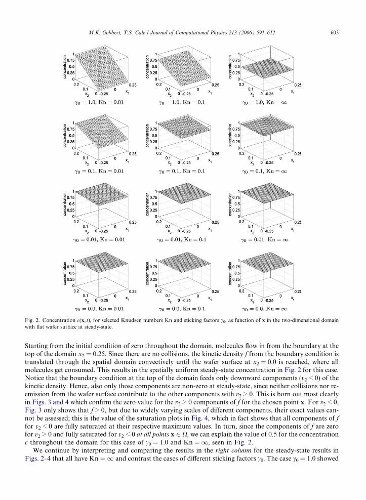
Fig. 2. Concentration c(x, t), for selected Knudsen numbers Kn and sticking factors c0, as function of x in the two-dimensional domainwith flat wafer surface at steady-state.


Starting from the initial condition of zero throughout the domain, molecules flow in from the boundary at thetop of the domain x2 = 0.25. Since there are no collisions, the kinetic density f from the boundary condition istranslated through the spatial domain convectively until the wafer surface at x2 = 0.0 is reached, where allmolecules get consumed. This results in the spatially uniform steady-state concentration in Fig. 2 for this case.Notice that the boundary condition at the top of the domain feeds only downward components (v2 < 0) of thekinetic density. Hence, also only those components are non-zero at steady-state, since neither collisions nor re-emission from the wafer surface contribute to the other components with v2 > 0. This is born out most clearlyin Figs. 3 and 4 which confirm the zero value for the v2 > 0 components of f for the chosen point x. For v2 < 0,Fig. 3 only shows that f > 0, but due to widely varying scales of different components, their exact values can-not be assessed; this is the value of the saturation plots in Fig. 4, which in fact shows that all components of ffor v2 < 0 are fully saturated at their respective maximum values. In turn, since the components of f are zerofor v2 > 0 and fully saturated for v2 < 0 at all points x 2 X, we can explain the value of 0.5 for the concentrationc throughout the domain for this case of c0 = 1.0 and Kn = 1, seen in Fig. 2.

We continue by interpreting and comparing the results in the right column for the steady-state results inFigs. 2–4 that all have Kn = 1 and contrast the cases of different sticking factors c0. The case c0 = 1.0 showed

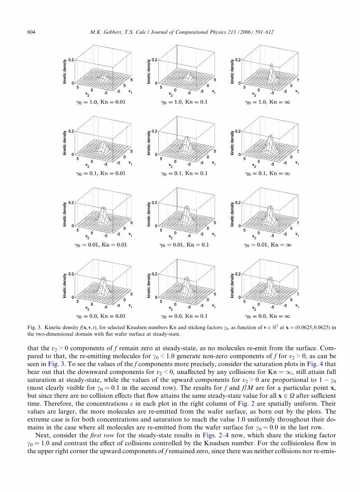
Fig. 3. Kinetic density f(x,v, t), for selected Knudsen numbers Kn and sticking factors c0, as function of v 2 R2 at x = (0.0625,0.0625) inthe two-dimensional domain with flat wafer surface at steady-state.


that the v2 > 0 components of f remain zero at steady-state, as no molecules re-emit from the surface. Com-pared to that, the re-emitting molecules for c0 < 1.0 generate non-zero components of f for v2 > 0, as can beseen in Fig. 3. To see the values of the f components more precisely, consider the saturation plots in Fig. 4 thatbear out that the downward components for v2 < 0, unaffected by any collisions for Kn = 1, still attain fullsaturation at steady-state, while the values of the upward components for v2 > 0 are proportional to 1 � c0(most clearly visible for c0 = 0.1 in the second row). The results for f and f/M are for a particular point x,but since there are no collision effects that flow attains the same steady-state value for all x 2 X after sufficienttime. Therefore, the concentrations c in each plot in the right column of Fig. 2 are spatially uniform. Theirvalues are larger, the more molecules are re-emitted from the wafer surface, as born out by the plots. Theextreme case is for both concentrations and saturation to reach the value 1.0 uniformly throughout their do-mains in the case where all molecules are re-emitted from the wafer surface for c0 = 0.0 in the last row.

Next, consider the first row for the steady-state results in Figs. 2–4 now, which share the sticking factorc0 = 1.0 and contrast the effect of collisions controlled by the Knudsen number. For the collisionless flow inthe upper right corner the upward components of f remained zero, since there was neither collisions nor re-emis-

Fig. 4. Saturation of kinetic density f(x,v, t)/M(v), for selected Knudsen numbers Kn and sticking factors c0, as function of v 2 R2 atx = (0.0625,0.0625) in the two-dimensional domain with flat wafer surface at steady-state.


sion from the wafer surface to contribute to them. Here, now, c0 = 1.0 implies that there are still no moleculesre-emitting from the wafer surface, but as Kn gets smaller, collisions become progressively more dominant andwe see non-zero f components for v2 > 0 in Fig. 3. The saturation plots in Fig. 4 clearly show the smoothing outthat results from progressively more collisions among the molecules, as more and more molecules collide toattain upward velocities as Kn decreases. To understand the concentration plots in Fig. 2, recall that all mol-ecules are consumed at the wafer surface at x2 = 0.0, hence the concentration must decrease from the top of thedomain to the wafer surface. This explains the spatial dependence seen in the plots. Moreover, since the upwardcomponents of f are solely fed by the collisions (as no molecules re-emit from the surface), this effect depends onthe location of the point x, with more contribution to all components of f the closer to the inflow at the top andthe more collisions (smaller Kn). This leads in turn to larger values of c at those locations, with the oppositeeffect the closer to the wafer surface at which molecules are consumed.

Consider now the last row of steady-state results in Figs. 2–4, which share the sticking factor c0 = 0.0. Forcollisionless transport with Kn = 1, a spatially uniform steady-state with full saturation of f was attained at


all points x 2 X, as the molecules flow from the top of the domain at x2 = 0.25 convectively without collisionsto the wafer surface at x0 = 0.0, where all of them get re-emitted. After sufficiently long time, this leads to thesaturation also of the upward components of f everywhere in X and a uniform concentration of 1.0. ForKn < 1 in the last row, collisions smooth out the kinetic density f from the start, leading to smaller numbersof molecules reaching the wafer surface than for Kn =1 at a fixed time. But after sufficiently long time, andthe smaller the Kn the longer time it takes, sufficiently many molecules have reached the wafer surface andhave been re-emitted from there to saturate all components of f, and we see that the case of c0 = 0.0 admitsa uniform Maxwellian steady-state solution. This is exhibited in the plots of c = 1.0 in Fig. 2 and full satura-tion in Fig. 4.

It remains to discuss the left and center columns for the second and third rows in Figs. 2–4: In those cases, wehave a combination of the effects of collisions and increasing re-emission of molecules from the wafer surface.Comparing the concentration plots in Fig. 2 for fixed Knudsen number shows the higher steady-state valuesattainable throughout the domain if less molecules are consumed. This reaches the extreme case of all mole-cules being re-emitted for c0 = 0.0 in the last row, where at steady-state the concentration attains its maximumvalue of 1.0 throughout the domain X. Fig. 3 bears out that all components of f are non-zero for collisionalregimes with Kn < 1, while Fig. 4 shows in more detail that collisions result in smoothing the kinetic densityas Kn decreases; compare the plots in the second row for c0 = 0.1. This tends to the extreme case, where nomolecules are consumed at the surface and then smoothed out by collisions, resulting in full saturation atsteady-state independent of the Knudsen number.

In summary, the concentration results in Fig. 2 show that the steady-state concentrations form a decreasingfunction from the top of the domain to the wafer surface, with the value at the wafer surface depending on thefraction of molecules that re-emit. But as c0 gets closer to 1.0 and a smaller fraction of molecules are re-emittedfrom the wafer surface, we see the effect of the transport regime characterized by the Knudsen number: thelarger Kn, the less interaction there is between the different velocity components in f, such that some of thecomponents remain zero in the extreme case of Kn = 1, thus limiting the concentration values attainableat steady-state. This behavior can only be explained in detail by considering the kinetic density f as a functionof its velocity arguments in Figs. 3 and 4. This demonstrates the value of being able to plot the kinetic densityas a function of its velocity arguments, because it provides more insight into the structure of the solution be-yond the macroscopic concentration as a function of space.

4.2. Application results for a three-dimensional irregular wafer surface

The results in Figs. 5–7 are designed to bring out the capabilities of the KTRM to simulate the transient

behavior of flow in a general domain X with irregular shape, such as the example shown in Fig. 1.We continue to use the single-species (ns = 1) sticking factor-based CVD model from the previous section

and contrast the results for three different Knudsen numbers Kn = 0.01, 0.1, and 1.0. The studies shown use asticking factor of c0 = 0.01, that is, 99% of all molecules re-emit from the surface. The results show the fol-lowing quantities:

Fig. 5: the dimensionless concentration 0 6 c(x, t) 6 1 as functions of x 2 X. Fig. 6: the kinetic density f(x,v, t)P 0 as functions of v 2 R3 at the mouth of the trench at x = (0.5,0.5, 0.0). Fig. 7: the saturation of the kinetic density 0 6 f(x,v, t)/M(v) 6 1 for (v1,v2) = (0,0) as functions of v3 2 R atmouth of the trench at x = (0.5,0.5, 0.0) and at mouth of the via at x = (0.5,0.5,�0.3).

For these transient studies, the figures show the results for the case of each Kn column-wise, indicated at thetop of the column, with each column showing the quantity at four different points in time, in re-dimension-alized units at t = 5, 10, 15, and 20 ns. These values are based on a reference time t* = 5 ns correspondingto a reference length L* = 1 lm and reference speed v* = 2.0 · 104 cm/s; this speed is appropriate for rel-atively high temperature T = 500 K and a relatively heavy reactant with molecular weight x of about200 g/mol.

It is challenging to display three-dimensional results in a meaningful and elucidating way and differentchoices are necessary for each quantity plotted. For each plot in Fig. 5, we choose to use a slice plot, which

Fig. 5. Slice plots of the dimensionless concentration c(x, t), for selected Knudsen numbers Kn at times t = 5, 10, 15, 20 ns, as function of xin the three-dimensional trench/via feature with slices at heights x3 = �0.60, �0.45, �0.30, �0.15, 0.00, 0.15. Grayscale fromlight () c = 0 to dark () c = 1.


encodes the values of 0 6 c(x, t) 6 1 for x 2 X on slices through X in grayscale from light color for c = 0 todark color for c = 1; simultaneously, a slice plot still gives an indication of the shape of the domain X bythe shapes of all slices taken together. We choose to show slice plots at 6 horizontal levels with heights ofx3 = �0.60, �0.45, �0.30, �0.15, 0.00, 0.15. The two top slices lie in the gaseous area of X above and atthe opening of the trench. The two middle layers lie inside the trench, as seen by the shape of the slices.The two bottom layers cut through the via below the trench, indicated by their shape as disks.

In the process considered here, gaseous chemicals are supplied from the gas-phase interface (at x3 = 0.3in Fig. 1) and flow downwards throughout the domain X until they reach the solid wafer surface (the surfaceplotted in Fig. 1 with flat parts at height x3 = 0.0), where a fraction of molecules react to form a solid deposit.Considering first the right column in Fig. 5 at time t = 5 ns, the top-most slice at x3 = 0.15 is mostly dark-colored, indicating that a relatively high concentration of molecules have reached this level from the inflowat the top of the domain. The slice at x3 = 0.0 shows that the concentration at the flat parts of the wafer

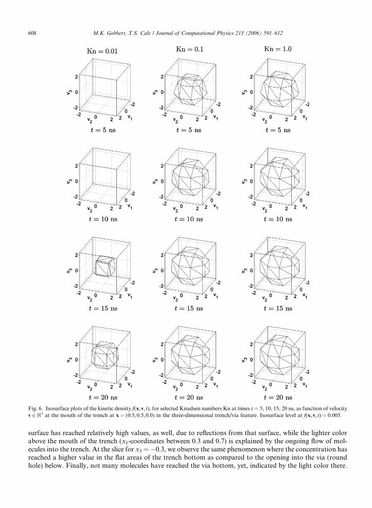
Fig. 6. Isosurface plots of the kinetic density f(x,v, t), for selected Knudsen numbers Kn at times t = 5, 10, 15, 20 ns, as function of velocityv 2 R3 at the mouth of the trench at x = (0.5,0.5,0.0) in the three-dimensional trench/via feature. Isosurface level at f(x,v, t) = 0.005.


surface has reached relatively high values, as well, due to reflections from that surface, while the lighter colorabove the mouth of the trench (x1-coordinates between 0.3 and 0.7) is explained by the ongoing flow of mol-ecules into the trench. At the slice for x3 = �0.3, we observe the same phenomenon where the concentration hasreached a higher value in the flat areas of the trench bottom as compared to the opening into the via (roundhole) below. Finally, not many molecules have reached the via bottom, yet, indicated by the light color there.

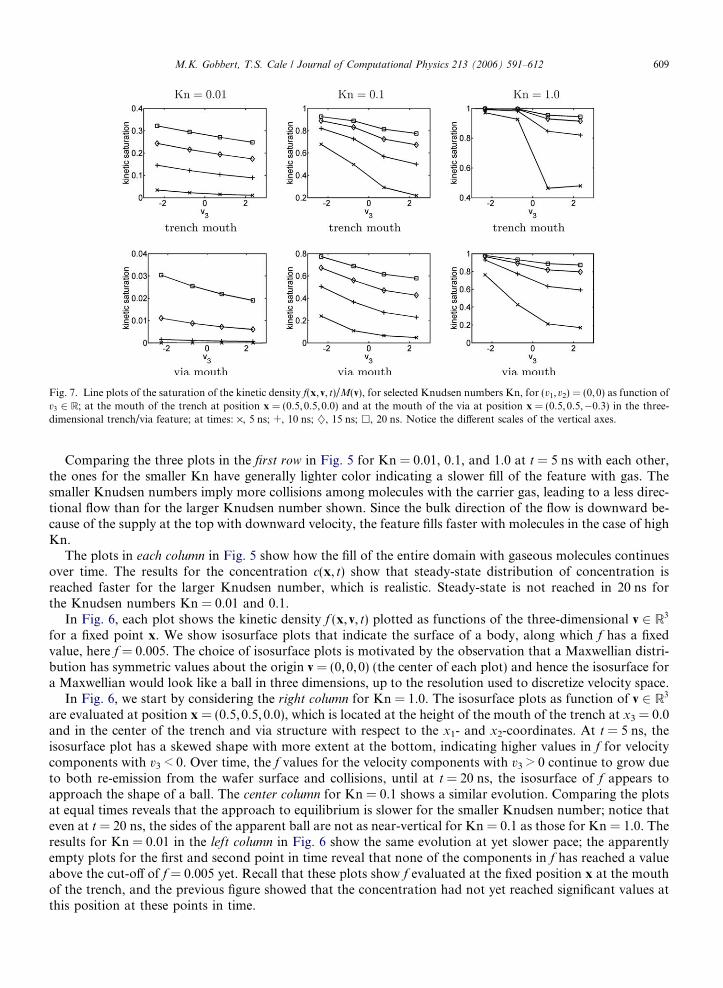
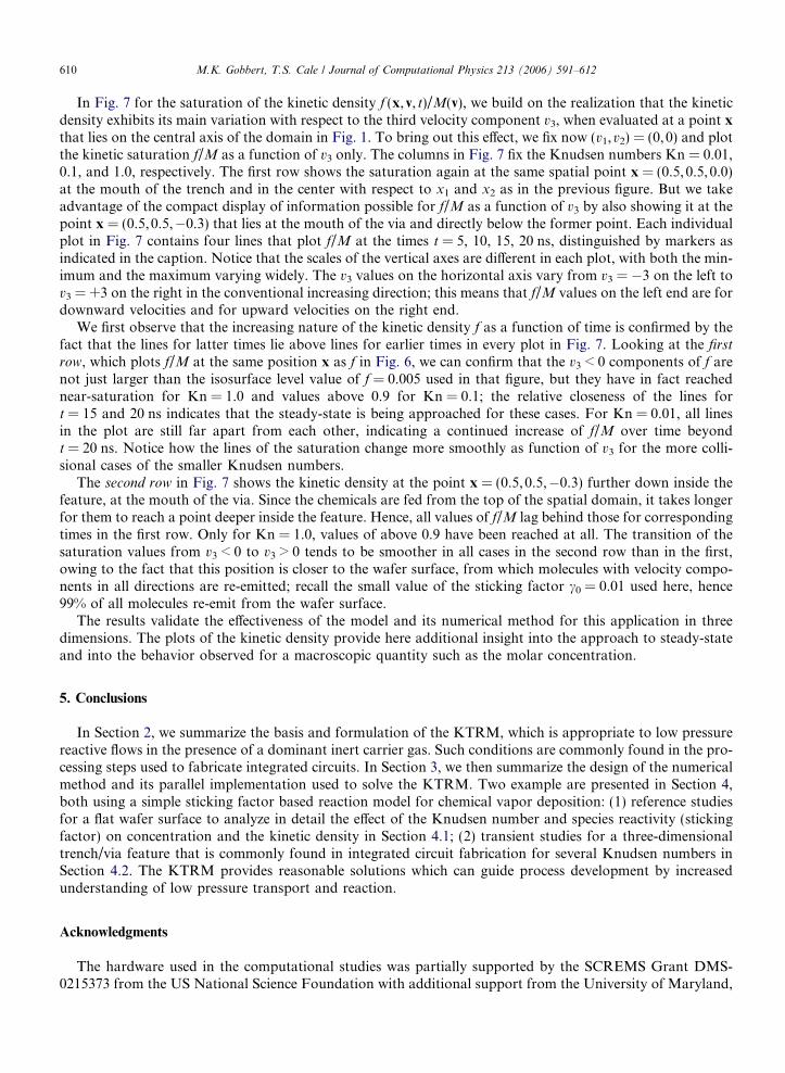
Fig. 7. Line plots of the saturation of the kinetic density f(x,v, t)/M(v), for selected Knudsen numbers Kn, for (v1,v2) = (0,0) as function ofv3 2 R; at the mouth of the trench at position x = (0.5,0.5,0.0) and at the mouth of the via at position x = (0.5,0.5,�0.3) in the three-dimensional trench/via feature; at times: ·, 5 ns; +, 10 ns; }, 15 ns; h, 20 ns. Notice the different scales of the vertical axes.


Comparing the three plots in the first row in Fig. 5 for Kn = 0.01, 0.1, and 1.0 at t = 5 ns with each other,the ones for the smaller Kn have generally lighter color indicating a slower fill of the feature with gas. Thesmaller Knudsen numbers imply more collisions among molecules with the carrier gas, leading to a less direc-tional flow than for the larger Knudsen number shown. Since the bulk direction of the flow is downward be-cause of the supply at the top with downward velocity, the feature fills faster with molecules in the case of highKn.

The plots in each column in Fig. 5 show how the fill of the entire domain with gaseous molecules continuesover time. The results for the concentration c(x, t) show that steady-state distribution of concentration isreached faster for the larger Knudsen number, which is realistic. Steady-state is not reached in 20 ns forthe Knudsen numbers Kn = 0.01 and 0.1.

In Fig. 6, each plot shows the kinetic density f (x,v, t) plotted as functions of the three-dimensional v 2 R3

for a fixed point x. We show isosurface plots that indicate the surface of a body, along which f has a fixedvalue, here f = 0.005. The choice of isosurface plots is motivated by the observation that a Maxwellian distri-bution has symmetric values about the origin v = (0,0,0) (the center of each plot) and hence the isosurface fora Maxwellian would look like a ball in three dimensions, up to the resolution used to discretize velocity space.

In Fig. 6, we start by considering the right column for Kn = 1.0. The isosurface plots as function of v 2 R3

are evaluated at position x = (0.5,0.5, 0.0), which is located at the height of the mouth of the trench at x3 = 0.0and in the center of the trench and via structure with respect to the x1- and x2-coordinates. At t = 5 ns, theisosurface plot has a skewed shape with more extent at the bottom, indicating higher values in f for velocitycomponents with v3 < 0. Over time, the f values for the velocity components with v3 > 0 continue to grow dueto both re-emission from the wafer surface and collisions, until at t = 20 ns, the isosurface of f appears toapproach the shape of a ball. The center column for Kn = 0.1 shows a similar evolution. Comparing the plotsat equal times reveals that the approach to equilibrium is slower for the smaller Knudsen number; notice thateven at t = 20 ns, the sides of the apparent ball are not as near-vertical for Kn = 0.1 as those for Kn = 1.0. Theresults for Kn = 0.01 in the left column in Fig. 6 show the same evolution at yet slower pace; the apparentlyempty plots for the first and second point in time reveal that none of the components in f has reached a valueabove the cut-off of f = 0.005 yet. Recall that these plots show f evaluated at the fixed position x at the mouthof the trench, and the previous figure showed that the concentration had not yet reached significant values atthis position at these points in time.


In Fig. 7 for the saturation of the kinetic density f (x,v, t)/M(v), we build on the realization that the kineticdensity exhibits its main variation with respect to the third velocity component v3, when evaluated at a point xthat lies on the central axis of the domain in Fig. 1. To bring out this effect, we fix now (v1,v2) = (0,0) and plotthe kinetic saturation f/M as a function of v3 only. The columns in Fig. 7 fix the Knudsen numbers Kn = 0.01,0.1, and 1.0, respectively. The first row shows the saturation again at the same spatial point x = (0.5,0.5,0.0)at the mouth of the trench and in the center with respect to x1 and x2 as in the previous figure. But we takeadvantage of the compact display of information possible for f/M as a function of v3 by also showing it at thepoint x = (0.5,0.5,�0.3) that lies at the mouth of the via and directly below the former point. Each individualplot in Fig. 7 contains four lines that plot f/M at the times t = 5, 10, 15, 20 ns, distinguished by markers asindicated in the caption. Notice that the scales of the vertical axes are different in each plot, with both the min-imum and the maximum varying widely. The v3 values on the horizontal axis vary from v3 = �3 on the left tov3 = +3 on the right in the conventional increasing direction; this means that f/M values on the left end are fordownward velocities and for upward velocities on the right end.

We first observe that the increasing nature of the kinetic density f as a function of time is confirmed by thefact that the lines for latter times lie above lines for earlier times in every plot in Fig. 7. Looking at the first

row, which plots f/M at the same position x as f in Fig. 6, we can confirm that the v3 < 0 components of f arenot just larger than the isosurface level value of f = 0.005 used in that figure, but they have in fact reachednear-saturation for Kn = 1.0 and values above 0.9 for Kn = 0.1; the relative closeness of the lines fort = 15 and 20 ns indicates that the steady-state is being approached for these cases. For Kn = 0.01, all linesin the plot are still far apart from each other, indicating a continued increase of f/M over time beyondt = 20 ns. Notice how the lines of the saturation change more smoothly as function of v3 for the more colli-sional cases of the smaller Knudsen numbers.

The second row in Fig. 7 shows the kinetic density at the point x = (0.5,0.5,�0.3) further down inside thefeature, at the mouth of the via. Since the chemicals are fed from the top of the spatial domain, it takes longerfor them to reach a point deeper inside the feature. Hence, all values of f/M lag behind those for correspondingtimes in the first row. Only for Kn = 1.0, values of above 0.9 have been reached at all. The transition of thesaturation values from v3 < 0 to v3 > 0 tends to be smoother in all cases in the second row than in the first,owing to the fact that this position is closer to the wafer surface, from which molecules with velocity compo-nents in all directions are re-emitted; recall the small value of the sticking factor c0 = 0.01 used here, hence99% of all molecules re-emit from the wafer surface.

The results validate the effectiveness of the model and its numerical method for this application in threedimensions. The plots of the kinetic density provide here additional insight into the approach to steady-stateand into the behavior observed for a macroscopic quantity such as the molar concentration.

5. Conclusions

In Section 2, we summarize the basis and formulation of the KTRM, which is appropriate to low pressurereactive flows in the presence of a dominant inert carrier gas. Such conditions are commonly found in the pro-cessing steps used to fabricate integrated circuits. In Section 3, we then summarize the design of the numericalmethod and its parallel implementation used to solve the KTRM. Two example are presented in Section 4,both using a simple sticking factor based reaction model for chemical vapor deposition: (1) reference studiesfor a flat wafer surface to analyze in detail the effect of the Knudsen number and species reactivity (stickingfactor) on concentration and the kinetic density in Section 4.1; (2) transient studies for a three-dimensionaltrench/via feature that is commonly found in integrated circuit fabrication for several Knudsen numbers inSection 4.2. The KTRM provides reasonable solutions which can guide process development by increasedunderstanding of low pressure transport and reaction.

Acknowledgments

The hardware used in the computational studies was partially supported by the SCREMS Grant DMS-0215373 from the US National Science Foundation with additional support from the University of Maryland,


Baltimore County. See www.math.umbc.edu/~gobbert/kali for more information on the machine and theprojects using it. Prof. Gobbert also wishes to thank the Institute for Mathematics and its Applications(IMA) at the University of Minnesota for its hospitality during Fall 2004. The IMA is supported by fundsprovided by the US National Science Foundation. Prof. Cale acknowledges support from MARCO, DARPA,and NYSTAR through the Interconnect Focus Center. We also thank Max O. Bloomfield for supplying theoriginal mesh of the trench/via structure.

References

[1] C. Bardos, F. Golse, C.D. Levermore, Fluid dynamics limits of kinetic equations II: convergence proofs for the Boltzmann equation,Commun. Pure Appl. Math. 46 (1993) 667–754.

[2] C.E. Baumann, J.T. Oden, An adaptive-order discontinuous Galerkin method for the solution of the Euler equations of gas dynamics,Int. J. Numer. Meth. Eng. 47 (2000) 61–73.

[3] G.A. Bird, Molecular Gas Dynamics, Oxford University Press, Oxford, 1976.[4] M.O. Bloomfield, T.S. Cale, Formation and evolution of grain structure in thin films, Micro. Eng. 76 (1–4) (2004) 195–

204.[5] T.S. Cale, M.O. Bloomfield, D.F. Richards, K.E. Jansen, M.K. Gobbert, Integrated multiscale process simulation, Comput. Mater.

Sci. 23 (2002) 3–14.[6] J.A. Carrillo, I.M. Gamba, A. Majorana, C.-W. Shu, A direct solver for 2D non-stationary Boltzmann–Poisson systems for

semiconductor devices: a MESFET simulation by WENO-Boltzmann schemes, J. Comput. Electron. 2 (2003) 375–380.[7] J.A. Carrillo, I.M. Gamba, A. Majorana, C.-W. Shu, A WENO-solver for the transients of Boltzmann–Poisson system for

semiconductor devices: performance and comparisons with Monte Carlo methods, J. Comput. Phys. 184 (2003) 498–525.[8] C. Cercignani, The Boltzmann Equation and Its Applications, Applied Mathematical Sciences, vol. 67, Springer, Berlin, 1988.[9] C. Cercignani, Rarefied Gas Dynamics: From Basic Concepts to Actual Calculations, Cambridge Texts in Applied Mathematics,

Cambridge University Press, Cambridge, 2000.[10] B. Cockburn, G.E. Karniadakis, C.-W. Shu (Eds.), Discontinuous Galerkin Methods: Theory, Computation and Applications,

Lecture Notes in Computational Science and Engineering, vol. 11, Springer, Berlin, 2000.[11] E. Fatemi, F. Odeh, Upwind finite difference solution of Boltzmann equation applied to electron transport in semiconductor devices,

J. Comput. Phys. 108 (1993) 209–217.[12] M.K. Gobbert, M.L. Breitenbach, T.S. Cale, Cluster computing for transient simulations of the linear Boltzmann equation on

irregular three-dimensional domains, in: V.S. Sunderam, G.D. van Albada, P.M.A. Sloot, J.J. Dongarra (Eds.), ComputationalScience—ICCS 2005, Lecture Notes in Computer Science, vol. 3516, Springer, Berlin, 2005, pp. 41–48.

[13] M.K. Gobbert, T.S. Cale, A feature scale transport and reaction model for atomic layer deposition, in: M.T. Swihart, M.D.Allendorf, M. Meyyappan (Eds.), Fundamental Gas-Phase and Surface Chemistry of Vapor-Phase Deposition II, vol. 2001-13, TheElectrochemical Society Proceedings Series, 2001, pp. 316–323.

[14] M.K. Gobbert, V. Prasad, T.S. Cale, Modeling and simulation of atomic layer deposition at the feature scale, J. Vac. Sci. Technol. B20 (3) (2002) 1031–1043.

[15] M.K. Gobbert, V. Prasad, T.S. Cale, Predictive modeling of atomic layer deposition on the feature scale, Thin Solid Films 410 (2002)129–141.

[16] M.K. Gobbert, S.G. Webster, T.S. Cale, Transient adsorption and desorption in micrometer scale features, J. Electrochem. Soc. 149(8) (2002) G461–G473.

[17] M.K. Gobbert, S.G. Webster, T.S. Cale, A Galerkin method for the simulation of the transient 2-D/2-D and 3-D/3-D linearBoltzmann equation, submitted (2005).

[18] A. Kersch, W.J. Morokoff, Transport Simulation in Microelectronics, Progress in Numerical Simulation for Microelectronics, vol. 3,Birkhauser Verlag, Basel, 1995.

[19] W.H. Reed, T.R. Hill, Triangular mesh methods for the neutron transport equation, Tech. Rep. LA-UR-73-479, Los AlamosScientific Laboratory, Los Alamos, NM, 1973.

[20] J.-F. Remacle, J.E. Flaherty, M.S. Shephard, An adaptive discontinuous Galerkin technique with an orthogonal basis applied tocompressible flow problems, SIAM Rev. 45 (1) (2003) 53–72.

[21] C. Ringhofer, Computational methods for semiclassical and quantum transport in semiconductor devices, Acta Numer. 6 (1997) 485–521.

[22] C. Ringhofer, Space–time discretization of series expansion methods for the Boltzmann transport equation, SIAM J. Numer. Anal. 38(2) (2000) 442–465.

[23] C. Ringhofer, C. Schmeiser, A. Zwirchmayr, Moment methods for the semiconductor Boltzmann equation on bounded positiondomains, SIAM J. Numer. Anal. 39 (3) (2001) 1078–1095.

[24] C. Schmeiser, A. Zwirchmayr, Convergence of moment methods for linear kinetic equations, SIAM J. Numer. Anal. 36 (1) (1998) 74–88.

[25] S.G. Webster, Stability and convergence of a spectral Galerkin method for the linear Boltzmann equation, Ph.D. thesis, University ofMaryland, Baltimore County, 2004.

http://www.math.umbc.edu/~gobbert/kali


[26] S.G. Webster, M.K. Gobbert, T.S. Cale, Transient 3-D/3-D transport and reactant-wafer interactions: Adsorption and desorption, in:P. Timans, E. Gusev, F. Roozeboom, M. Ozturk, D.L. Kwong (Eds.), Rapid Thermal and Other Short-Time Processing TechnologiesIII, vol. 2002-11, The Electrochemical Society Proceedings Series, 2002, pp. 81–88.

[27] S.G. Webster, M.K. Gobbert, J.-F. Remacle, T.S. Cale, Parallel numerical solution of the Boltzmann equation for atomic layerdeposition, in: B. Monien, R. Feldmann (Eds.), Euro-Par 2002 Parallel Processing, Lecture Notes in Computer Science, vol. 2400,Springer, Berlin, 2002, pp. 452–456.

a kinetic transport and reaction model and simulator for ...gobbert/papers/gobbertcalejcp2006.pdfa...

Documents