analysis of kinetic reaction mechanisms

Tamás Turányi · Alison S. Tomlin

Analysis of Kinetic Reaction Mechanisms

Analysis of Kinetic Reaction Mechanisms

ThiS is a FM Blank Page

Tamas Turanyi • Alison S. Tomlin

Analysis of Kinetic ReactionMechanisms

Tamas TuranyiInstitute of ChemistryEotvos UniversityBudapestHungary

Alison S. TomlinSchool of Chemical and Process EngineeringUniversity of LeedsLeedsUnited Kingdom

ISBN 978-3-662-44561-7 ISBN 978-3-662-44562-4 (eBook)DOI 10.1007/978-3-662-44562-4Springer Heidelberg New York Dordrecht London

Library of Congress Control Number: 2014957310

© Springer-Verlag Berlin Heidelberg 2014This work is subject to copyright. All rights are reserved by the Publisher, whether the whole or partof the material is concerned, specifically the rights of translation, reprinting, reuse of illustrations,recitation, broadcasting, reproduction on microfilms or in any other physical way, and transmission orinformation storage and retrieval, electronic adaptation, computer software, or by similar or dissimilarmethodology now known or hereafter developed. Exempted from this legal reservation are brief excerptsin connection with reviews or scholarly analysis or material supplied specifically for the purpose of beingentered and executed on a computer system, for exclusive use by the purchaser of the work. Duplicationof this publication or parts thereof is permitted only under the provisions of the Copyright Law of thePublisher’s location, in its current version, and permission for use must always be obtained fromSpringer. Permissions for use may be obtained through RightsLink at the Copyright Clearance Center.Violations are liable to prosecution under the respective Copyright Law.The use of general descriptive names, registered names, trademarks, service marks, etc. in thispublication does not imply, even in the absence of a specific statement, that such names are exemptfrom the relevant protective laws and regulations and therefore free for general use.While the advice and information in this book are believed to be true and accurate at the date ofpublication, neither the authors nor the editors nor the publisher can accept any legal responsibility forany errors or omissions that may be made. The publisher makes no warranty, express or implied, withrespect to the material contained herein.

Printed on acid-free paper

Springer is part of Springer Science+Business Media (www.springer.com)

Contents

1 Introduction . . . . . . . . . . . . . . . . . . . . . . . . . . . . . . . . . . . . . . . . . . 1

References . . . . . . . . . . . . . . . . . . . . . . . . . . . . . . . . . . . . . . . . . . . . 3

2 Reaction Kinetics Basics . . . . . . . . . . . . . . . . . . . . . . . . . . . . . . . . . 5

2.1 Stoichiometry and Reaction Rate . . . . . . . . . . . . . . . . . . . . . . . 5

2.1.1 Reaction Stoichiometry . . . . . . . . . . . . . . . . . . . . . . . 5

2.1.2 Molecularity of an Elementary Reaction . . . . . . . . . . . 9

2.1.3 Mass Action Kinetics and Chemical Rate Equations . . . 10

2.1.4 Examples . . . . . . . . . . . . . . . . . . . . . . . . . . . . . . . . . 14

2.2 Parameterising Rate Coefficients . . . . . . . . . . . . . . . . . . . . . . . 18

2.2.1 Temperature Dependence of Rate Coefficients . . . . . . . 18

2.2.2 Pressure Dependence of Rate Coefficients . . . . . . . . . . 20

2.2.3 Reversible Reaction Steps . . . . . . . . . . . . . . . . . . . . . 26

2.3 Basic Simplification Principles in Reaction Kinetics . . . . . . . . . 28

2.3.1 The Pool Chemical Approximation . . . . . . . . . . . . . . . 28

2.3.2 The Pre-equilibrium Approximation . . . . . . . . . . . . . . 29

2.3.3 Rate-Determining Step . . . . . . . . . . . . . . . . . . . . . . . . 30

2.3.4 The Quasi-Steady-State Approximation (QSSA) . . . . . 30

2.3.5 Conserved Properties . . . . . . . . . . . . . . . . . . . . . . . . . 32

2.3.6 Lumping of Reaction Steps . . . . . . . . . . . . . . . . . . . . . 33

References . . . . . . . . . . . . . . . . . . . . . . . . . . . . . . . . . . . . . . . . . . . . 34

3 Mechanism Construction and the Sources of Data . . . . . . . . . . . . . 39

3.1 Automatic Mechanism Generation . . . . . . . . . . . . . . . . . . . . . . 39

3.2 Data Sources . . . . . . . . . . . . . . . . . . . . . . . . . . . . . . . . . . . . . 46

References . . . . . . . . . . . . . . . . . . . . . . . . . . . . . . . . . . . . . . . . . . . . 48

v

4 Reaction Pathway Analysis . . . . . . . . . . . . . . . . . . . . . . . . . . . . . . . 53

4.1 Species Conversion Pathways . . . . . . . . . . . . . . . . . . . . . . . . . 53

4.2 Pathways Leading to the Consumption or Production

of a Species . . . . . . . . . . . . . . . . . . . . . . . . . . . . . . . . . . . . . . 56

References . . . . . . . . . . . . . . . . . . . . . . . . . . . . . . . . . . . . . . . . . . . . 59

5 Sensitivity and Uncertainty Analyses . . . . . . . . . . . . . . . . . . . . . . . 61

5.1 Introduction . . . . . . . . . . . . . . . . . . . . . . . . . . . . . . . . . . . . . . 61

5.2 Local Sensitivity Analysis . . . . . . . . . . . . . . . . . . . . . . . . . . . . 63

5.2.1 Basic Equations . . . . . . . . . . . . . . . . . . . . . . . . . . . . . 63

5.2.2 The Brute Force Method . . . . . . . . . . . . . . . . . . . . . . 66

5.2.3 The Green Function Method . . . . . . . . . . . . . . . . . . . . 67

5.2.4 The Decoupled Direct Method . . . . . . . . . . . . . . . . . . 68

5.2.5 Automatic Differentiation . . . . . . . . . . . . . . . . . . . . . . 69

5.2.6 Application to Oscillating Systems . . . . . . . . . . . . . . . 70

5.3 Principal Component Analysis of the Sensitivity Matrix . . . . . . 71

5.4 Local Uncertainty Analysis . . . . . . . . . . . . . . . . . . . . . . . . . . . 74

5.5 Global Uncertainty Analysis . . . . . . . . . . . . . . . . . . . . . . . . . . 75

5.5.1 Morris Screening Method . . . . . . . . . . . . . . . . . . . . . . 76

5.5.2 Global Uncertainty Analysis Using Sampling-Based

Methods . . . . . . . . . . . . . . . . . . . . . . . . . . . . . . . . . . 79

5.5.3 Sensitivity Indices . . . . . . . . . . . . . . . . . . . . . . . . . . . 86

5.5.4 Fourier Amplitude Sensitivity Test . . . . . . . . . . . . . . . 88

5.5.5 Response Surface Methods . . . . . . . . . . . . . . . . . . . . . 90

5.5.6 Moment-Independent Global Sensitivity Analysis

Methods . . . . . . . . . . . . . . . . . . . . . . . . . . . . . . . . . . 100

5.6 Uncertainty Analysis of Gas Kinetic Models . . . . . . . . . . . . . . 101

5.6.1 Uncertainty of the Rate Coefficients . . . . . . . . . . . . . . 102

5.6.2 Characterisation of the Uncertainty of the Arrhenius

Parameters . . . . . . . . . . . . . . . . . . . . . . . . . . . . . . . . . 106

5.6.3 Local Uncertainty Analysis of Reaction Kinetic

Models . . . . . . . . . . . . . . . . . . . . . . . . . . . . . . . . . . . 111

5.6.4 Examples of the Application of Uncertainty Analysis to

Methane Flame Models . . . . . . . . . . . . . . . . . . . . . . . 114

5.6.5 Applications of Response Surface Techniques to

Uncertainty Analysis in Gas Kinetic Models . . . . . . . . 119

5.6.6 Handling Correlated Inputs Within Global Uncertainty

and Sensitivity Studies . . . . . . . . . . . . . . . . . . . . . . . . 123

5.7 Uncertainty Analysis in Systems Biology . . . . . . . . . . . . . . . . . 124

Uncertainty Analysis: General Conclusions . . . . . . . . . . . . . . . . . . . . 128

References . . . . . . . . . . . . . . . . . . . . . . . . . . . . . . . . . . . . . . . . . . . . 133

6 Timescale Analysis . . . . . . . . . . . . . . . . . . . . . . . . . . . . . . . . . . . . . 145

6.1 Introduction . . . . . . . . . . . . . . . . . . . . . . . . . . . . . . . . . . . . . . 145

6.2 Species Lifetimes and Timescales . . . . . . . . . . . . . . . . . . . . . . 146

vi Contents

6.3 Application of Perturbation Theory to Chemical Kinetic

Systems . . . . . . . . . . . . . . . . . . . . . . . . . . . . . . . . . . . . . . . . . 152

6.4 Computational Singular Perturbation Theory . . . . . . . . . . . . . . 160

6.5 Slow Manifolds in the Space of Variables . . . . . . . . . . . . . . . . 163

6.6 Timescales in Reactive Flow Models . . . . . . . . . . . . . . . . . . . . 169

6.7 Stiffness of Reaction Kinetic Models . . . . . . . . . . . . . . . . . . . . 171

6.8 Operator Splitting and Stiffness . . . . . . . . . . . . . . . . . . . . . . . . 175

References . . . . . . . . . . . . . . . . . . . . . . . . . . . . . . . . . . . . . . . . . . . . 177

7 Reduction of Reaction Mechanisms . . . . . . . . . . . . . . . . . . . . . . . . 183

7.1 Introduction . . . . . . . . . . . . . . . . . . . . . . . . . . . . . . . . . . . . . . 184

7.2 Reaction Rate and Jacobian-Based Methods for Species

Removal . . . . . . . . . . . . . . . . . . . . . . . . . . . . . . . . . . . . . . . . 185

7.2.1 Species Removal via the Inspection of Rates . . . . . . . . 185

7.2.2 Species Elimination via Trial and Error . . . . . . . . . . . . 186

7.2.3 Connectivity Method: Connections Between the Species

Defined by the Jacobian . . . . . . . . . . . . . . . . . . . . . . . 187

7.2.4 Simulation Error Minimization Connectivity

Method . . . . . . . . . . . . . . . . . . . . . . . . . . . . . . . . . . . 188

7.3 Identification of Redundant Reaction Steps Using Rate-of-

Production and Sensitivity Methods . . . . . . . . . . . . . . . . . . . . . 189

7.4 Identification of Redundant Reaction Steps Based on Entropy

Production . . . . . . . . . . . . . . . . . . . . . . . . . . . . . . . . . . . . . . . 192

7.5 Graph-Based Methods . . . . . . . . . . . . . . . . . . . . . . . . . . . . . . . 193

7.5.1 Directed Relation Graph Method . . . . . . . . . . . . . . . . 193

7.5.2 DRG-Aided Sensitivity Analysis . . . . . . . . . . . . . . . . . 197

7.5.3 DRG with Error Propagation . . . . . . . . . . . . . . . . . . . 198

7.5.4 The Path Flux Analysis Method . . . . . . . . . . . . . . . . . 200

7.5.5 Comparison of Methods for Species Elimination . . . . . 201

7.6 Optimisation Approaches . . . . . . . . . . . . . . . . . . . . . . . . . . . . 202

7.6.1 Integer Programming Methods . . . . . . . . . . . . . . . . . . 202

7.6.2 Genetic Algorithm-Based Methods . . . . . . . . . . . . . . . 206

7.6.3 Optimisation of Reduced Models to Experimental

Data . . . . . . . . . . . . . . . . . . . . . . . . . . . . . . . . . . . . . 208

7.6.4 Application to Oscillatory Systems . . . . . . . . . . . . . . . 209

7.7 Species Lumping . . . . . . . . . . . . . . . . . . . . . . . . . . . . . . . . . . 210

7.7.1 Chemical Lumping . . . . . . . . . . . . . . . . . . . . . . . . . . 211

7.7.2 Linear Lumping . . . . . . . . . . . . . . . . . . . . . . . . . . . . . 217

7.7.3 Linear Lumping in Systems with Timescale

Separation . . . . . . . . . . . . . . . . . . . . . . . . . . . . . . . . . 222

7.7.4 General Nonlinear Methods . . . . . . . . . . . . . . . . . . . . 224

7.7.5 Approximate Nonlinear Lumping in Systems with

Timescale Separation . . . . . . . . . . . . . . . . . . . . . . . . . 226

Contents vii

7.7.6 Continuous Lumping . . . . . . . . . . . . . . . . . . . . . . . . . 227

7.7.7 The Application of Lumping to Biological and

Biochemical Systems . . . . . . . . . . . . . . . . . . . . . . . . . 229

7.8 The Quasi-Steady-State Approximation . . . . . . . . . . . . . . . . . . 231

7.8.1 Basic Equations . . . . . . . . . . . . . . . . . . . . . . . . . . . . . 232

7.8.2 Historical Context . . . . . . . . . . . . . . . . . . . . . . . . . . . 233

7.8.3 The Analysis of Errors . . . . . . . . . . . . . . . . . . . . . . . . 234

7.8.4 Further Recent Approaches to the Selection of

QSS-Species . . . . . . . . . . . . . . . . . . . . . . . . . . . . . . . 238

7.8.5 Application of the QSSA in Spatially Distributed

Systems . . . . . . . . . . . . . . . . . . . . . . . . . . . . . . . . . . . 239

7.8.6 Practical Applications of the QSSA . . . . . . . . . . . . . . . 240

7.9 CSP-Based Mechanism Reduction . . . . . . . . . . . . . . . . . . . . . . 242

7.10 Numerical Reduced Models Derived from the Rate Equations of

the Detailed Model . . . . . . . . . . . . . . . . . . . . . . . . . . . . . . . . . 244

7.10.1 Slow Manifold Methods . . . . . . . . . . . . . . . . . . . . . . . 245

7.10.2 Intrinsic Low-Dimensional Manifolds . . . . . . . . . . . . . 247

7.10.3 Application of ILDM Methods in Reaction Diffusion

Systems . . . . . . . . . . . . . . . . . . . . . . . . . . . . . . . . . . . 251

7.10.4 Thermodynamic Approaches for the Calculation of

Manifolds . . . . . . . . . . . . . . . . . . . . . . . . . . . . . . . . . 253

7.11 Numerical Reduced Models Based on Geometric

Approaches . . . . . . . . . . . . . . . . . . . . . . . . . . . . . . . . . . . . . . 257

7.11.1 Calculation of Slow Invariant Manifolds . . . . . . . . . . . 257

7.11.2 The Minimal Entropy Production Trajectory

Method . . . . . . . . . . . . . . . . . . . . . . . . . . . . . . . . . . . 259

7.11.3 Calculation of Temporal Concentration Changes Based

on the Self-Similarity of the Concentration Curves . . . 259

7.12 Tabulation Approaches . . . . . . . . . . . . . . . . . . . . . . . . . . . . . . 260

7.12.1 The Use of Look-Up Tables . . . . . . . . . . . . . . . . . . . . 261

7.12.2 In Situ Tabulation . . . . . . . . . . . . . . . . . . . . . . . . . . . 263

7.12.3 Controlling Errors and the Invariant Constrained

Equilibrium Pre-image Curve (ICE-PIC) Method . . . . . 267

7.12.4 Flamelet-Generated Manifolds . . . . . . . . . . . . . . . . . . 270

7.13 Numerical Reduced Models Based on Fitting . . . . . . . . . . . . . . 271

7.13.1 Calculation of Temporal Concentration Changes Using

Difference Equations . . . . . . . . . . . . . . . . . . . . . . . . . 272

7.13.2 Calculation of Concentration Changes by Assuming the

Presence of Slow Manifolds . . . . . . . . . . . . . . . . . . . . 274

7.13.3 Fitting Polynomials Using Factorial Design . . . . . . . . . 275

7.13.4 Fitting Polynomials Using Taylor Expansions . . . . . . . 276

7.13.5 Orthonormal Polynomial Fitting Methods . . . . . . . . . . 276

7.13.6 High-Dimensional Model Representations . . . . . . . . . . 281

viii Contents

7.13.7 Artificial Neural Networks . . . . . . . . . . . . . . . . . . . . . 282

7.13.8 Piecewise Reusable Maps (PRISM) . . . . . . . . . . . . . . 286

7.14 Adaptive Reduced Mechanisms . . . . . . . . . . . . . . . . . . . . . . . . 287

References . . . . . . . . . . . . . . . . . . . . . . . . . . . . . . . . . . . . . . . . . . . . 291

8 Similarity of Sensitivity Functions . . . . . . . . . . . . . . . . . . . . . . . . . 313

8.1 Introduction and Basic Definitions . . . . . . . . . . . . . . . . . . . . . . 313

8.2 The Origins of Local Similarity and Scaling Relationships . . . . 316

8.3 The Origin of Global Similarity . . . . . . . . . . . . . . . . . . . . . . . . 322

8.4 Similarity of the Sensitivity Functions of Biological Models . . . 325

8.5 The Importance of the Similarity of Sensitivity Functions . . . . . 330

References . . . . . . . . . . . . . . . . . . . . . . . . . . . . . . . . . . . . . . . . . . . . 335

9 Computer Codes for the Study of Complex Reaction Systems . . . . 337

9.1 General Simulation Codes in Reaction Kinetics . . . . . . . . . . . . 337

9.2 Simulation of Gas Kinetics Systems . . . . . . . . . . . . . . . . . . . . . 339

9.3 Analysis of Reaction Mechanisms . . . . . . . . . . . . . . . . . . . . . . 342

9.4 Investigation of Biological Reaction Kinetic Systems . . . . . . . . 344

9.5 Global Uncertainty Analysis . . . . . . . . . . . . . . . . . . . . . . . . . . 347

References . . . . . . . . . . . . . . . . . . . . . . . . . . . . . . . . . . . . . . . . . . . . 349

10 Summary and Concluding Remarks . . . . . . . . . . . . . . . . . . . . . . . . 353

Index . . . . . . . . . . . . . . . . . . . . . . . . . . . . . . . . . . . . . . . . . . . . . . . . . . . 359

Contents ix

Chapter 1

Introduction

Abstract Chemical processes can be described by detailed kinetic reaction mech-

anisms consisting of several hundreds or even thousands of reaction steps. Such

reaction mechanisms are used in many fields of science and technology, including

combustion, atmospheric chemistry, environmental modelling, process engineer-

ing, and systems biology. This book describes methods for the analysis of reaction

mechanisms that are applicable in all these fields. The book will address topics such

as the importance of model evaluation as well as the need for model reduction under

situations where the kinetic model is coupled with models describing complex

physical processes where computational expense becomes a critical issue. It

includes topics such as: the basic foundations of chemical kinetic models; methods

for the automatic generation of kinetic mechanisms; sources of thermodynamic and

kinetic data; methods for uncertainty and sensitivity analysis; timescale analyses;

similarities in model sensitivities; and chemical model reduction. Within the

introduction we discuss the motivations behind the text as well as providing a

brief summary of key reference texts on similar topics from the current literature.

Chemical processes can be described by detailed kinetic reaction mechanisms

consisting of several hundreds or even thousands of reaction steps. Detailed reac-

tion mechanisms are used in many fields of science and technology, including

combustion, atmospheric chemistry, environmental modelling, process engineering

and systems biology. This book describes methods for the analysis of reaction

mechanisms that are applicable in all these fields. The reasons for analysis may

vary. It may be important to determine the key reaction steps that drive the overall

reactivity of the chemical system or the production of key species. It may also be

necessary to include the chemical mechanism within a larger model describing, for

example, a reactive flow problem. In this case, the smallest version of the mecha-

nism describing key kinetic features may be required in order to meet the limita-

tions of the computational requirements. Mechanism reduction techniques can

identify the core reactions in a large mechanism and the application of reduced

mechanisms may speed up the simulations, allowing engineering optimisations. It

may also be important to determine the predictability of any model which incor-

porates the chemical mechanism and therefore to assess the confidence that can be

placed in simulation results. Uncertainty analysis allows the calculation of the

uncertainty of simulation results based on the users’ best knowledge of the input

© Springer-Verlag Berlin Heidelberg 2014

T. Turanyi, A.S. Tomlin, Analysis of Kinetic Reaction Mechanisms,DOI 10.1007/978-3-662-44562-4_1

1

parameters, potentially putting an error bar on model predictions. Sensitivity

analysis can provide the subsequent identification of the most important parameters

driving model uncertainty. These methods can form a key part of the process of

model evaluation and improvement.

This book is a monograph for researchers and engineers dealing with detailed

kinetic reaction mechanisms and also a textbook for graduate students of related

courses in chemistry, mechanical engineering, environmental science and biology.

We include biology, since nowadays even biological and biochemical processes

such as the cell cycle, metabolism networks and molecular signal transfer can be

described by detailed reaction mechanisms (Klipp et al. 2005, 2009). Reaction

kinetic formalism is also used in some ecological models. The best-known example

is the Lotka�Volterra model (Lotka 1910, 1920; Volterra 1926), which describes

the dynamics of a biological system consisting of an interaction of a predator and a

prey. This model was originally suggested by Lotka to describe autocatalytic

chemical reactions, but the same equations were later interpreted to model

predator–prey interactions. Erdi and Toth (1989) also claim that reaction kinetic

formalisms are frequently used as a metalanguage in many other fields. The

methods described in this book are all applicable for the analysis of non-chemical

models that use chemical kinetic formalism. Moreover, many of the methods should

be applicable without substantial modifications, for the analysis of any model based

on differential equations used in physics, chemistry, biology or economics.

Several reviews dealing with the topics of this book have previously been

published. The book chapter of Tomlin et al. (1997) discusses many relevant papers

that were published up to 1995 that dealt with mathematical and computational

methods used for the automatic creation, analysis and reduction of detailed reaction

mechanisms in combustion. Several journal review articles have also subsequently

been published (Okino and Mavrovouniotis 1998; Ross and Vlad 1999; Law

et al. 2003; Law 2007; Ross 2008; Lu and Law 2009; Pope 2013; Stagni

et al. 2014) that discuss various available methods for the analysis and reduction

of reaction mechanisms. The book chapter of Goussis andMaas also confers several

mechanism reduction methods, especially those that are related to turbulent com-

bustion modelling (Goussis and Maas 2011). Mathematical modelling of chemical

reactions was discussed in the book of Erdi and Toth (1989). Mechanism reduction

methods based on invariant manifolds are described in the book of Gorban and

Karlin (2005). Volume 42 of series Comprehensive Chemical Kinetics (Carr 2007)

contains several related reviews dealing with topics such as an introduction to

chemical kinetics and the construction and optimisation of reaction mechanisms.

Part IV [Chaps. 16 to 19; (Tomlin and Turanyi 2013a, b; Maas and Tomlin 2013;

Turanyi and Tomlin 2013)] of a book on the development of detailed chemical

kinetic models for cleaner combustion (Battin-Leclerc et al. 2013) deals with

several topics of this book, including methods for mechanism reduction and

uncertainty analysis.

The various methods used for sensitivity analysis are discussed in several recent

reviews (Saltelli et al. 2005, 2006, 2012; Saltelli and Annoni 2010; Zi 2011;

Tomlin 2013; Wang and Sheen 2015), a monograph (Saltelli et al. 2000) and two

2 1 Introduction

http://en.wikipedia.org/wiki/Dynamical_system#Dynamical%20system

http://en.wikipedia.org/wiki/Systems_biology#Systems%20biology

http://dx.doi.org/10.1007/978-3-662-44562-4_16

http://dx.doi.org/10.1007/978-3-662-44562-4_19

textbooks (Saltelli et al. 2004, 2008). This book aims to bring together and update

the discussion of a wide range of techniques available for the analysis of chemical

kinetic mechanisms and to guide the user on the most appropriate techniques for

different classes of problems.

References

Battin-Leclerc, F., Blurock, E., Simmie, J. (eds.): Development of Detailed Chemical Kinetic

Models for Cleaner Combustion. Springer, Heidelberg (2013)

Carr, R.W. (ed.): Modeling of Chemical Reactions. Elsevier, Amsterdam (2007)

Erdi, P., Toth, J.: Mathematical Models of Chemical Reactions. Princeton University Press,

Princeton (1989)

Gorban, A., Karlin, I.V.: Invariant Manifolds for Physical and Chemical Kinetics. Springer, Berlin

(2005)

Goussis, D.A., Maas, U.: Model reduction for combustion chemistry. In: Echekki, T., Mastorakos,

E. (eds.) Turbulent Combustion Modeling, pp. 193–220. Springer, New York (2011)

Klipp, E., Herwig, R., Kowald, A., Wierling, C., Lehrach, H.: Systems Biology in Practice. Wiley-

VCH, Weinheim (2005)

Klipp, E., Liebermeister, W., Wierling, C., Kowland, A., Lehrach, H., Herwig, R.: Systems

Biology: A Textbook. Wiley-VCH Verlag, Weinheim (2009)

Law, C.K.: Combustion at a crossroads: status and prospects. Proc. Combust Inst. 31, 1–29 (2007)Law, C.K., Sung, C.J., Wang, H., Lu, T.F.: Development of comprehensive detailed and reduced

reaction mechanisms for combustion modeling. AIAA J. 41, 1629–1646 (2003)

Lotka, A.J.: Contribution to the theory of periodic reaction. J. Phys. Chem. 14, 271–274 (1910)

Lotka, A.J.: Analytical note on certain rhythmic relations in organic systems. Proc. Natl. Acad.

Sci. U. S. A. 6, 410–415 (1920)

Lu, T., Law, C.K.: Toward accommodating realistic fuel chemistry in large-scale computations.

Prog. Energy Combust. Sci. 35, 192–215 (2009)

Maas, U., Tomlin, A.S.: Time-scale splitting-based mechanism reduction. In: Battin-Leclerc, F.,

Blurock, E., Simmie, J. (eds.) Development of Detailed Chemical Kinetic Models for Cleaner

Combustion, pp. 467–484. Springer, Heidelberg (2013)

Okino, M.S., Mavrovouniotis, M.L.: Simplification of mathematical models of chemical reaction

systems. Chem. Rev. 98, 391–408 (1998)

Pope, S.B.: Small scales, many species and the manifold challenges of turbulent combustion. Proc.

Combust. Inst. 34, 1–31 (2013)

Ross, J.: Determination of complex reaction mechanisms. Analysis of chemical, biological and

genetic networks. J. Phys. Chem. A 112, 2134–2143 (2008)

Ross, J., Vlad, M.O.: Nonlinear kinetics and new approaches to complex reaction mechanisms.

Ann. Rev. Phys. Chem. 50, 51–78 (1999)

Saltelli, A., Annoni, P.: How to avoid a perfunctory sensitivity analysis. Environ. Model. Software

25, 1508–1517 (2010)

Saltelli, A., Scott, M., Chen, K. (eds.): Sensitivity Analysis. Wiley, Chichester (2000)

Saltelli, A., Tarantola, S., Campolongo, F., Ratto, M.: Sensitivity Analysis in Practice. A Guide to

Assessing Scientific Models. Wiley, Chichester (2004)

Saltelli, A., Ratto, M., Tarantola, S., Campolongo, F.: Sensitivity analysis for chemical models.

Chem. Rev. 105, 2811–2828 (2005)

Saltelli, A., Ratto, M., Tarantola, S., Campolongo, F.: Sensitivity analysis practices: strategies for

model-based inference. Reliab. Eng. Syst. Saf. 91, 1109–1125 (2006)

Saltelli, A., Ratto, M., Andres, T., Campolongo, F., Cariboni, J., Gatelli, D., Saisana, M.,

Tarantola, S.: Global Sensitivity Analysis: The Primer. Wiley, New York (2008)

References 3

Saltelli, A., Ratto, M., Tarantola, S., Campolongo, F.: Update 1 of: sensitivity analysis for

chemical models. Chem. Rev. 112, PR1–PR21 (2012)

Stagni, A., Cuoci, A., Frassoldati, A., Faravelli, T., Ranzi, E.: Lumping and reduction of detailed

kinetic schemes: an effective coupling. Ind. Eng. Chem. Res. 53, 9004–9016 (2014)

Tomlin, A.S.: The role of sensitivity and uncertainty analysis in combustion modelling. Proc.

Combust. Inst. 34, 159–176 (2013)

Tomlin, A.S., Turanyi, T.: Investigation and improvement of reaction mechanisms using sensi-

tivity analysis and optimization. In: Battin-Leclerc, F., Blurock, E., Simmie, J. (eds.) Devel-

opment of Detailed Chemical Kinetic Models for Cleaner Combustion, pp. 411–445. Springer,

Heidelberg (2013a)

Tomlin, A.S., Turanyi, T.: Mechanism reduction to skeletal form and species lumping. In: Battin-

Leclerc, F., Blurock, E., Simmie, J. (eds.) Development of Detailed Chemical Kinetic Models

for Cleaner Combustion, pp. 447–466. Springer, Heidelberg (2013b)

Tomlin, A.S., Turanyi, T., Pilling, M.J.: Mathematical tools for the construction, investigation and

reduction of combustion mechanisms. In: Pilling, M.J., Hancock, G. (eds.) Low-temperature

Combustion and Autoignition. Comprehensive Chemical Kinetics, vol. 35, pp. 293–437.

Elsevier, Amsterdam (1997)

Turanyi, T., Tomlin, A.S.: Storage of chemical kinetic information. In: Battin-Leclerc, F.,

Blurock, E., Simmie, J. (eds.) Development of Detailed Chemical Kinetic Models for Cleaner

Combustion, pp. 485–512. Springer, Heidelberg (2013)

Volterra, V.: Variazioni e fluttuazioni del numero d’individui in specie animali conviventi. Mem.

Acad. Lincei Roma 2, 31–113 (1926)

Wang, H., Sheen, D.A.: Combustion kinetic model uncertainty quantification, propagation and

minimization. Prog. Energy Combust. Sci. 47, 1–31 (2015)

Zi, Z.: Sensitivity analysis approaches applied to systems biology models. IET Syst. Biol. 5, 336–346 (2011)

4 1 Introduction

Chapter 2

Reaction Kinetics Basics

Abstract This chapter provides an introduction to the basic concepts of reaction

kinetics simulations. The level corresponds mainly to undergraduate teaching in

chemistry and in process, chemical and mechanical engineering. However, some

topics are discussed in more detail and depth in order to underpin the later chapters.

The section “parameterising rate coefficients” contains several topics that are

usually not present in textbooks. For example, all reaction kinetics textbooks

discuss the pressure dependence of the rate coefficients of unimolecular reactions,

but usually do not cover those of complex-forming bimolecular reactions. The

chapter contains an undergraduate level introduction to basic simplification princi-

ples in reaction kinetics. The corresponding sections also discuss the handling of

conserved properties in chemical kinetic systems and the lumping of reaction steps.

2.1 Stoichiometry and Reaction Rate

2.1.1 Reaction Stoichiometry

In this section, we begin by explaining the formulation of chemical reaction

mechanisms and the process of setting up chemical rate equations from stoichio-

metric information and elementary reaction rates.

First, we assume that a chemical process can be described by a single stoichio-metric equation. The stoichiometric equation defines the molar ratio of the reacting

species and the reaction products. This equation is also called the overall reactionequation. Real chemical systems corresponding to such a single chemical reaction,

that is, when the reactants react with each other forming products immediately, are

in fact very rare. In most cases, the reaction of the reactants produces intermediates,

these intermediates react with each other and the reactants, and the final products

are formed at the end of many coupled reaction steps. Each of the individual steps is

called an elementary reaction. Within elementary reactions, there is no macro-

scopically observable intermediate between the reactants and the products. This

point is now illustrated for the case of hydrogen oxidation, but similar examples

could be cited across many different application fields.



5

The overall reaction equation of the production of water from hydrogen and

oxygen is very simple:

2H2 þ O2 ¼ 2H2O:

We can see that this overall reaction balances the quantities of the different

elements contained in the reactants and products of the reaction. Reaction stoichio-

metry describes the 2:1:2 ratio of hydrogen, oxygen and water molecules in the

above equation. From a stoichiometric point of view, a chemical equation can be

rearranged, similarly to a mathematical equation. For example, all terms can be

shifted to the right-hand side:

0 ¼ �2H2 � 1O2 þ 2H2O:

Let us denote the formulae of the chemical species by the vector A¼ (A1, A2, A3)

and the corresponding multiplication factors by vector ν¼ (v1, v2, v3). In this case,

A1¼ “H2”, A2¼ “O2”, A3¼ “H2O” and v1¼�2, v2¼�1, v3¼ +2. The

corresponding general stoichiometric equation is

0 ¼XNS

j¼1

vjAj; ð2:1Þ

where NS is the number of species. The general stoichiometric equation of any

chemical process can be defined in a similar way, where vj is the stoichiometriccoefficient of the jth species and Aj is the formula of the jth species in the overall

reaction equation. The stoichiometric coefficients are negative for the reactants and

positive for the products. The stoichiometric coefficients define the ratios of the

reactants and products. Therefore, these are uncertain according to a scalar multi-

plication factor. This means that by multiplying all stoichiometric coefficients with

the same scalar, the resulting chemical equation refers to the same chemical

process. Thus, chemical equations 0¼ –2H2 – 1O2 + 2H2O and 0¼ –1H2 –½O2+ 1H2O (or using the traditional notation, 2H2 +O2¼ 2H2O and

H2 +½O2¼H2O, respectively) represent the same chemical process. Also, the

order of the numbering of the species is arbitrary. We show here the stoichiometric

coefficients for an overall reaction step, but the same approach is taken for each of

the elementary steps of a detailed chemical scheme. In general, for elementary

reaction steps within a chemical mechanism, the stoichiometric coefficients are

integers.

There are many chemical processes for which a single overall reaction equation

that describes the stoichiometry of the process cannot be found. For example, the

oxidation of hydrocarbons sourced from exhaust gases in the troposphere cannot be

described by a single overall reaction equation. Many types of hydrocarbons are

emitted to the troposphere, and their ratio changes dependent on the type of

6 2 Reaction Kinetics Basics

pollution source. Therefore, no single species can be identified as reactants or

products.

Let us now think about the time-dependent behaviour of a chemical system and

how we might describe it using information from the kinetic reaction system. The

simplest practical case here would be one or more reactants reacting in a well-

mixed vessel to form one or more products over time. In this case, if the molar

concentration Yj of the jth species is measured at several consecutive time points,

then by applying a finite-difference approach, the production rate of the jth speciesdYj/dt can be calculated. The rate of a chemical reaction defined by stoichiometric

equation (2.1) is the following:

r ¼ 1

vj

dYj

dt: ð2:2Þ

Reaction rate r is independent of index j. This means that the same reaction rate is

obtained when the production rate of any of the species is measured. However, the

reaction rate depends on the stoichiometric coefficient, and therefore, the reaction

rate depends on a given form of the stoichiometric equation.

Within a narrow range of concentrations, the reaction rate r can always be

approximated by the following equation:

r ¼ kYNS

j¼1

Yjαj ; ð2:3Þ

where the positive scalar k is called the rate coefficient, the exponents αj are positivereal numbers or zero, the operator Π means that the product of all terms behind it

should be calculated and NS is the number of species. In the case of some reactions,

the form of Eq. (2.3) is applicable over a wide range of concentrations. When the

reaction rate is calculated by Eq. (2.3), molar concentrations (i.e. the amount of

matter divided by volume with units such as mol cm�3) should always be used. The

rate coefficient k is independent of the concentrations but may depend on temper-

ature, pressure and the quality and quantity of the nonreactive species present

(e.g. an inert dilution gas or a solvent). This is the reason why the widely used

term rate constant is not preferred and rate coefficient is a more appropriate term.

The exponent αj in Eq. (2.3) is called the reaction order with respect to species Aj.

The sum of these exponents α ¼XNS

j¼1

αj

!is called the overall order of the

reaction. In the case of an overall reaction equation such as 2H2 +O2¼ 2H2O, the

order αj is usually not equal to the stoichiometric coefficient vj because of the

intermediate steps that are involved in the overall reaction. For elementary reac-

tions, the reaction orders of the reactions and the absolute value of the stoichio-

metric coefficients of the reactants are commonly mathematically the same.

2.1 Stoichiometry and Reaction Rate 7

As stated above, intermediates are formed within most reaction systems, and

hence, in order to define the time-dependent dynamics of a system accurately, a

reaction model should include steps where such intermediates are formed from

reactants and then go on to form products. For example, detailed reaction mecha-

nisms for the oxidation of hydrogen [see e.g. O Conaire et al. (2004), Konnov

(2008), Hong et al. (2011), Burke et al. (2012), Varga et al. (2015)] contain not only

the reactants (H2 and O2) and the product (H2O) but also several intermediates

(H, O, OH, HO2, H2O2), which are present in the 30–40 reaction steps considered.

Any hydrogen combustion mechanism should contain the following reaction steps:

R1 H2 þ O2 ¼ Hþ HO2 k1R2 O2 þ H ¼ OHþ O k2R3 H2 þ OH ¼ Hþ H2O k3R4 H2 þ O ¼ Hþ OH k4R5 O2 þ HþM ¼ HO2 þM k5R6 HO2 þ OH ¼ H2Oþ OH k6

;

where species M represents any species present in the mixture and will be further

discussed in the next section.

The number of elementary reaction steps within a kinetic reaction mechanism

can typically vary from ten to several ten thousands, depending on the chemical

process, the reaction conditions and the required detail and accuracy of the chem-

ical kinetic model. Each elementary reaction step i can be characterised by the

following stoichiometric equation:Xj

vLijAj ¼Xj

vRijAj; ð2:4Þ

where the stoichiometric coefficients on the left-hand side (vLij) and the right-hand

side (vRij) of an elementary reaction step should be distinguished. The stoichiometric

coefficient belonging to species i in a reaction step can be obtained from the

equation vij¼ vRij � vLij. The left-hand side stoichiometric coefficients vLij should be

positive integers, whilst the right-hand side stoichiometric coefficients vRij are

positive integers for elementary reactions and can be positive or negative, integer

or real numbers for reaction steps that were obtained by the combination

(“lumping”) of several elementary reactions. Therefore, the overall stoichiometric

coefficients vij can also be any numbers (positive or negative figures; integers or real

numbers). Elements vLij, vRij and vij constitute the left-hand side, the right-hand side

and the overall stoichiometric matrix, respectively.To emphasise the analogy with mathematical equations, so far the equality sign

(¼) was always used for chemical equations. From now on, arrows will be used for

one-way or irreversible chemical reactions (like A!B). Reversible reactions will

be denoted by double arrows (like A⇄B).


A detailed kinetic reaction mechanism contains the stoichiometric equations of

type (2.4) and the corresponding rate coefficient for each reaction step. These rate

coefficients can be physical constants that are valid for the conditions of the

reactions (e.g. temperature, pressure) or functions that can be used to calculate

the value of the rate coefficient applicable at the actual temperature, pressure, gas

composition, etc. The physical dimension of the rate coefficient depends on the

overall order of the reaction step. When the order of the reaction step is 0, 1, 2 or

3, the dimension of the rate coefficient is concentration� (time)�1, (time)�1,

(concentration)�1� (time)�1 or (concentration)�2� ( time)�1, respectively.

2.1.2 Molecularity of an Elementary Reaction

The reaction steps in the mechanism of a homogeneous gas-phase reaction are

usually elementary reactions, that is, the stoichiometric equation of the reaction

step corresponds to real molecular changes. The molecularity of an elementary

reaction is the number of molecular entities involved in the molecular encounter.

Thus, an elementary reaction can be unimolecular or bimolecular. Some books on

chemical kinetics also discuss termolecular reactions (Raj 2010), but three molec-

ular entities colliding at the same time is highly improbable (Drake 2005). What are

often referred to as termolecular reactions actually involve the formation of an

energetically excited reaction intermediate in a bimolecular reaction which can then

collide with a third molecular entity (e.g. a molecule or radical).

In a unimolecular reaction, only one reaction partner species is changed. Exam-

ples include photochemical reactions (e.g. NO2+ hν!NO+O, where hν repre-

sents a photon) and unimolecular decomposition such as the decomposition of fuel

molecules in combustion or pyrolysis. In such reactions, the fuel molecule decom-

poses as a result of collision with another molecule that does not change chemically

during the molecular event (e.g. C3H8 +N2!CH3 +C2H5 +N2). The

rearrangement of a molecule such as the isomerisation of gas-phase molecules

and the fluctuation of the structure of a protein from one conformation to another

are also results of such so-called nonreactive collisions (Bamford et al. 1969).

Most elementary reactions are bimolecular, when two particles (molecules,

radicals, ions) meet and both particles change chemically. Bimolecular reactions

can be either direct bimolecular reactions (e.g. H2+OH!H+H2O) or complex-

forming bimolecular reactions (e.g. O2+H!HO2* and HO2* +M!HO2+M). In

direct bimolecular reactions, the products are formed in a single step. The product

of a complex-forming bimolecular reaction is a highly energised intermediate

(in this case, a vibrationally excited HO2 radical) that has to lose the excess energy

in another collision with any other particle called a third-body M. This third body

can be a molecule of the bath gas (in most experiments argon or nitrogen) or any

other species of the reaction system. A more detailed description on how the

reaction steps involving third bodies are treated is presented in Sect. 2.2.2.


http://en.wikipedia.org/wiki/Molecular_entity#Molecular%20entity

In this section, we have discussed elementary reaction steps, but there are many

reaction mechanisms where the reaction steps are not elementary reactions, but

lumped reactions. This is very common, for example, in solution-phase kinetics and

will be discussed in detail later.

The distinction between molecularity and order is an important one. It is

therefore important that the terms unimolecular reaction and first-order reaction,

and bimolecular reaction and second-order reaction are not synonyms. The first

term refers to a type of molecular change whilst the second one to the type of

applicable rate equation governed by the observed dependence of reaction rates on

concentration.

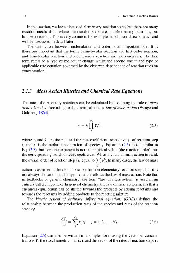
2.1.3 Mass Action Kinetics and Chemical Rate Equations

The rates of elementary reactions can be calculated by assuming the rule of massaction kinetics. According to the chemical kinetic law of mass action (Waage and

Guldberg 1864)

ri ¼ kiYNS

j

Yjν Lij ; ð2:5Þ

where ri and ki are the rate and the rate coefficient, respectively, of reaction step

i, and Yj is the molar concentration of species j. Equation (2.5) looks similar to

Eq. (2.3), but here the exponent is not an empirical value (the reaction order), but

the corresponding stoichiometric coefficient. When the law of mass action is valid,

the overall order of reaction step i is equal toXj

νLij . In many cases, the law of mass

action is assumed to be also applicable for non-elementary reaction steps, but it is

not always the case that a lumped reaction follows the law of mass action. Note that

in textbooks of general chemistry, the term “law of mass action” is used in an

entirely different context. In general chemistry, the law of mass action means that a

chemical equilibrium can be shifted towards the products by adding reactants and

towards the reactants by adding products to the reacting mixture.

The kinetic system of ordinary differential equations (ODEs) defines the

relationship between the production rates of the species and rates of the reaction

steps ri:

dYj

dt¼XNR

i

νijri; j ¼ 1, 2, . . . ,NS: ð2:6Þ

Equation (2.6) can also be written in a simpler form using the vector of concen-

trations Y, the stoichiometric matrix ν and the vector of the rates of reaction steps r:


dY

dt¼ νr: ð2:7Þ

This means that the number of equations in the kinetic systems of ODEs is equal

to the number of species in the reaction mechanism. These equations are coupled

and therefore can only be solved simultaneously. It is also generally true that in

order to accurately represent the time-dependent behaviour of a chemical system,

the ODEs should be based on the chemical mechanism incorporating intermediate

species and elementary reaction steps rather than the overall reaction equation

which contains only reactants and products. We will see later in Chap. 7 that one

aim of chemical mechanism reduction is to limit the number of required interme-

diates within the mechanism in order to reduce the number of ODEs required to

accurately represent the time-dependent behaviour of key species.

An analogous equation to Eq. (2.6) can be written when other concentration

units are used, e.g. mass fractions or mole fractions [see, e.g. Warnatz et al. (2006)],

but Eq. (2.5) is applicable only when the “amount of matter divided by volume”

concentration units are used. The amount of matter can be defined, e.g., in moles or

molecules, whilst volume is usually defined in dm3 or cm3 units.

In adiabatic systems or in systems with a known heat loss rate, usually temper-

ature is added as the (NS + 1)th variable of the kinetic system of ODEs. The

differential equation for the rate of change of temperature in a closed spatially

homogeneous reaction vessel is given as

Cp

dT

dt¼XNR

i¼1

ΔrH⦵i ri � χS

VT � T0ð Þ; ð2:8Þ

where T is the actual temperature of the system, T0 is the ambient temperature

(e.g. the temperature of the lab), Cp is the constant pressure heat capacity of the

mixture, ΔrH⦵i is the standard molar reaction enthalpy of reaction step i, S and V are

the surface and the volume of the system, respectively, and χ is the heat transfer

coefficient between the system and its surroundings. The change in temperature can

be calculated together with the change in concentrations as part of the coupled ODE

system. In the examples used throughout the book, the variables of the kinetic

differential equations will be species concentrations only, but in all cases, the ODE

can be easily extended to include the equation for temperature.

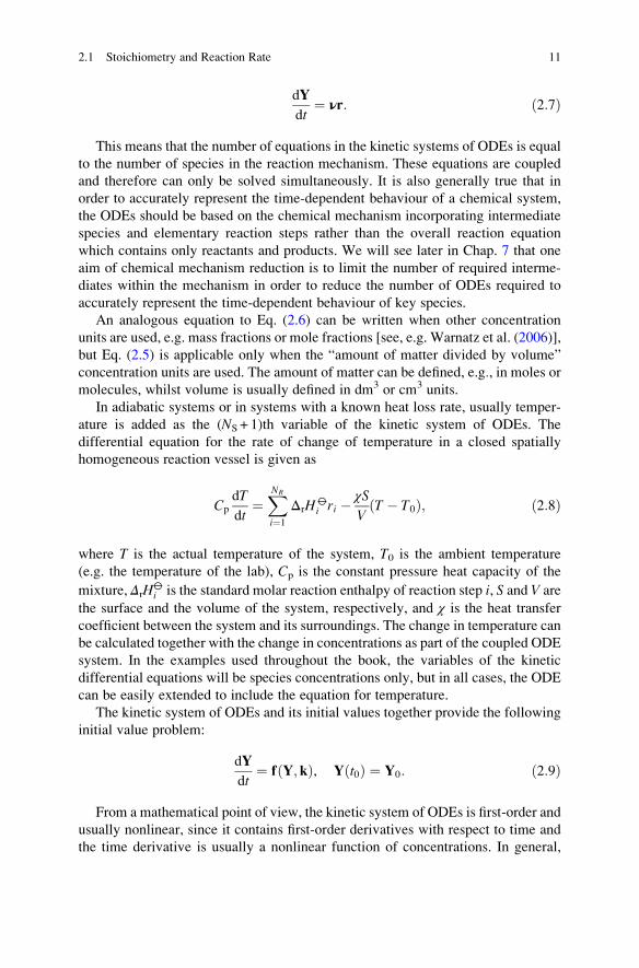
The kinetic system of ODEs and its initial values together provide the following

initial value problem:

dY

dt¼ f Y; kð Þ, Y t0ð Þ ¼ Y0: ð2:9Þ

From a mathematical point of view, the kinetic system of ODEs is first-order and

usually nonlinear, since it contains first-order derivatives with respect to time and

the time derivative is usually a nonlinear function of concentrations. In general,


http://dx.doi.org/10.1007/978-3-662-44562-4_7

each species participates in several reactions; therefore, the production rates of the

species are coupled. The rates of the reaction steps can be very different and may

span many (even 10–25) orders of magnitude. Such differential equations are called

stiff ODEs. The stiffness of the kinetic ODEs and related problems will be

discussed in detail in Sect. 6.7.

In theory, if a laboratory experiment is repeated say one hour later than the first

execution, then the same concentration–time curves should be obtained (ignoring

experimental error for now). Accordingly, the time in the kinetic system of differ-

ential equations is not the wall-clock time, but a relative time from the beginning of

the experiment. Such a differential equation system is called an autonomous systemof ODEs. In other cases, such as in atmospheric chemical or biological circadian

rhythm models, the actual physical time is important, because a part of the param-

eters (the rate coefficients belonging to the photochemical reactions) depend on the

strength of sunshine, which is a function of the absolute time. In this case, the

kinetic system of ODEs is nonautonomous.Great efforts are needed even in a laboratory to achieve a homogeneous spatial

distribution of the concentrations, temperature and pressure of a system, even in a

small volume (a few mm3 or cm3). Outside the confines of the laboratory, chemical

processes always occur under spatially inhomogeneous conditions, where the

spatial distribution of the concentrations and temperature is not uniform, and

transport processes also have to be taken into account. Therefore, reaction kinetic

simulations frequently include the solution of partial differential equations that

describe the effect of chemical reactions, material diffusion, thermal diffusion,

convection and possibly turbulence. In these partial differential equations, the

term f defined on the right-hand side of Eq. (2.9) is the so-called chemical source

term. In the remainder of the book, we deal mainly with the analysis of this

chemical source term rather than the full system of model equations.

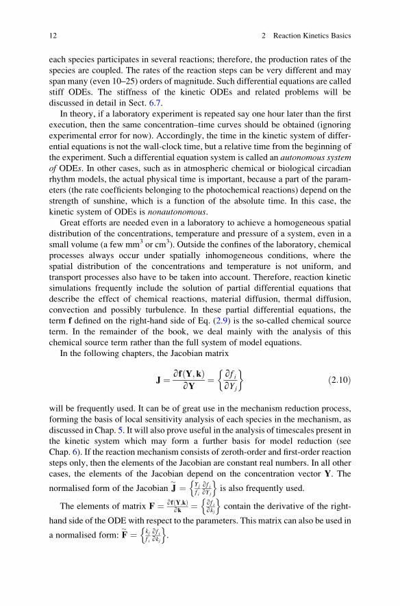
In the following chapters, the Jacobian matrix

J ¼ ∂f Y; kð Þ∂Y

¼ ∂f i∂Yj

� �ð2:10Þ

will be frequently used. It can be of great use in the mechanism reduction process,

forming the basis of local sensitivity analysis of each species in the mechanism, as

discussed in Chap. 5. It will also prove useful in the analysis of timescales present in

the kinetic system which may form a further basis for model reduction (see

Chap. 6). If the reaction mechanism consists of zeroth-order and first-order reaction

steps only, then the elements of the Jacobian are constant real numbers. In all other

cases, the elements of the Jacobian depend on the concentration vector Y. The

normalised form of the Jacobian J� ¼ Yj

f i

∂f i∂Yj

n ois also frequently used.

The elements of matrix F ¼ ∂f Y;kð Þ∂k ¼ ∂f i

∂kj

n ocontain the derivative of the right-

hand side of the ODE with respect to the parameters. This matrix can also be used in

a normalised form: F� ¼ kj

f i

∂f i∂kj

n o.


http://dx.doi.org/10.1007/978-3-662-44562-4_6#Sec7

http://dx.doi.org/10.1007/978-3-662-44562-4_5

http://dx.doi.org/10.1007/978-3-662-44562-4_6

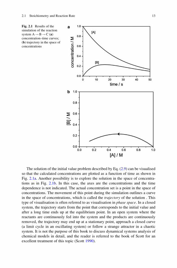
The solution of the initial value problem described by Eq. (2.9) can be visualised

so that the calculated concentrations are plotted as a function of time as shown in

Fig. 2.1a. Another possibility is to explore the solution in the space of concentra-

tions as in Fig. 2.1b. In this case, the axes are the concentrations and the time

dependence is not indicated. The actual concentration set is a point in the space of

concentrations. The movement of this point during the simulation outlines a curve

in the space of concentrations, which is called the trajectory of the solution . This

type of visualisation is often referred to as visualisation in phase space. In a closed

system, the trajectory starts from the point that corresponds to the initial value and

after a long time ends up at the equilibrium point. In an open system where the

reactants are continuously fed into the system and the products are continuously

removed, the trajectory may end up at a stationary point, approach a closed curve

(a limit cycle in an oscillating system) or follow a strange attractor in a chaotic

system. It is not the purpose of this book to discuss dynamical systems analysis of

chemical models in detail, and the reader is referred to the book of Scott for an

excellent treatment of this topic (Scott 1990).

Fig. 2.1 Results of the

simulation of the reaction

system A!B!C (a)concentration–time curves;

(b) trajectory in the space ofconcentrations


If the mechanism consists of only first-order reaction steps, then the kinetic

system of ODEs always has a solution which can be expressed in the form of

mathematical functions (Rodiguin and Rodiguina 1964). Such a solution is called

analytical in science and engineering and symbolic in the literature of mathematics

and computer science. The analytical solution of small reaction mechanisms,

consisting of mixed first-order and second-order steps, can also be found in the

chapter of Szabo (1969) and the reaction kinetics chapter of Atkins’ Physical

Chemistry textbook (Atkins and de Paula 2009). However, in most practical

cases, for larger coupled kinetic systems, finding analytical solutions is not possible

without seeking simplifications of the chemistry representation. In most cases

therefore, numerical solutions of the kinetic differential equations (2.9) are sought.

Reaction kinetic models can be simulated not only on a deterministic basis by

solving the kinetic system of differential equations but also via the simulation of

stochastic models (Erdi et al. 1973; Bunker et al. 1974; Erdi and Toth 1976;

Gillespie 1976, 1977; Toth and Erdi 1978; Kraft and Wagner 2003; Gillespie

2007; Li et al. 2008; Tomlin et al. 1994). If the system contains many molecules,

then the two solutions usually (but not always) provide identical solutions (Kurtz

1972). If the system contains few molecules, which frequently occurs in biological

systems, then the stochastic solution can be qualitatively different from the deter-

ministic one (Aranyi and Toth 1977). Stochastic chemical kinetic modelling is

discussed in detail in a recent monograph (Erdi and Lente 2014) .

2.1.4 Examples

The first example for the creation of the kinetic system of ODEs will be based on a

skeleton hydrogen combustion mechanism. Using the law of mass action, the rates

r1 to r6 of the reaction steps can be calculated from the species concentrations and

rate coefficients

R1 H2 þ O2 ! H þ HO2 k1 r1 ¼ k1 H2½ � O2½ �R2 O2 þ H ! OH þ O k2 r2 ¼ k2 O2½ � H½ �R3 H2 þ OH ! H þ H2O k3 r3 ¼ k3 H2½ � OH½ �R4 H2 þ O ! H þ OH k4 r4 ¼ k4 H2½ � O½ �R5 O2 þ H þ M ! HO2 þ M k5 r5 ¼ k5 O2½ � H½ � M½ �R6 HO2 þ OH ! H2O þ OH k6 r6 ¼ k6 HO2½ � OH½ �

:

Here [M] is the sum of the concentrations of all species present. The species that are

jointly denoted by M may have a different effective concentration than their actual

physical concentration based on how effective their collisions are in making

reaction R5 proceed (see Sect. 2.2.2).

The calculation of the production rates is based on Eq. (2.6). For example, the

hydrogen atom H is produced in reaction steps 1, 3 and 4 (v¼ +1), it is consumed in

reaction steps 2 and 5 (v¼�1), and it is not present in reaction step 6 (v¼ 0). The


line of the kinetic system of ODEs, corresponding to the production of H is the

following:

d H½ �dt

¼ þ1r1 � 1r2 þ r3 þ 1r4 � 1r5 þ 0r6;

or

d H½ �dt

¼ k1 H2½ � O2½ � � k2 O2½ � H½ � þ k3 H2½ � OH½ � þ k4 H2½ � O½ � � k5 O2½ � H½ � M½ �:

In a similar way, the production of water can be described by the following

equations:

d H2O½ �dt

¼ þ1r3 þ 1r6;

or

d H2O½ �dt

¼ k3 H2½ � OH½ � þ k6 HO2½ � OH½ �:

Let us now consider a more complex mechanism, where the stoichiometric

coefficients are not only �1, 0 or +1. Whilst the hydrogen oxidation example is

very simple, the next example contains all possible complications. We now illus-

trate the formulation of the kinetic ODEs and their related matrices on an example

based on the well-known Belousov–Zhabotinskii (BZ) reaction. The BZ reaction

has been highly studied as an example of non-equilibrium thermodynamics where a

nonlinear chemical oscillator can easily be established in a simple reaction vessel

and illustrated by a simple colour change. The starting mixture consists of potas-

sium bromate, malonic acid and a cerium (IV) salt in an acidic solution. A

simplified mechanism of the BZ oscillating reaction (Belousov 1959; Zhabotinsky

1964; Belousov 1985) was elaborated by Field et al. (1972). The Oregonator model

(Field and Noyes 1974) was based on this mechanism. A newer version (Turanyi

et al. 1993) of the reaction steps within the Oregonator model is the following:

R1 X þ Y ! 2 P k1 r1 ¼ k1xyR2 Y þ A ! X þ P k2 r2 ¼ k2yaR3 2 X ! P þ A k3 r3 ¼ k3x

2

R4 X þ A ! 2 X þ 2 Z k4 r4 ¼ k4xaR5 X þ Z ! 0:5 X þ A k5 r5 ¼ k5xzR6 Z þ Ma ! Y � Z k6 r6 ¼ k6zm

;

where X, Y, Z, A, P and Ma indicate species HBrO2, Br�, Ce4+, BrO3

�, HOBr andmalonic acid, respectively. The corresponding small italic letter denotes the molar


concentration of the species and k1,. . ., k6 the rate coefficients of the reaction steps.

The rates of the reaction steps (r1,. . .,r6) can be calculated using the kinetic law of

mass action [Eq. (2.5)] even though not all reactions in this reduced scheme could

be classified as elementary reaction steps. Note, for example, that reactions 5 and

6 do not contain positive whole integers as stoichiometric coefficients on the right-

hand side. The concentrations of species BrO3� (A) and malonic acid (Ma) are

much higher than those of the others, and these concentrations are practically

constant (this is termed the pool chemical approximation, and it is detailed in

Sect. 2.3.1). Note that HOBr (P) is considered as a nonreactive product.

In the models of formal reaction kinetics, a species is called an internal species ifits concentration change is important for the simulation of the reaction system.

These species are denoted by letters from the end of the Latin alphabet (X, Y, Z).

The concentrations of the external species are either constant or change slowly in

time (A and Ma) (pool chemical) or have no effect on the concentrations of the

other species (P).

According to this model, the rates of change of the concentrations of HBrO2 (X),

Br� (Y) and Ce4+ (Z) in a well-mixed closed vessel are described by the following

system of ODEs:

dx

dt¼ �1r1 þ 1r2 � 2r3 þ 1r4 � 0:5r5;

dy

dt¼ �1r1 � 1r2 þ 1r6;

dz

dt¼ þ2r4 � 1r5 � 2r6:

In each equation, on the right-hand side in each term, the rate of the reaction step

is multiplied by the change in the number of moles in the corresponding chemical

equation. For example, one mole of species X is consumed in reaction step

1 (therefore, the change in the number of moles is �1); in reaction step 2, one

mole of X is produced (+1); and in step 3, two moles are consumed (�2). In reaction

step 4, one mole of X is consumed and two moles are produced; therefore, the

change in the number of moles is +1.

Inserting the terms for the reaction rates r1 – r6 into the equations above gives

dx

dt¼ �k1xyþ k2ya� 2k3x

2 þ k4xa� 0:5k5xz;

dy

dt¼ �k1xy� k2yaþ k6zm;

dz

dt¼ 2k4xa� k5xz� 2k6zm:

Some remarks should be made concerning the equations above. Species concen-

tration ci has to be present in all negative terms on the right-hand side of the


equation dci/dt. A negative term without concentration ci is called a negative crosseffect (Erdi and Toth 1989). A first-order ordinary system of differential equations

with polynomial right-hand side can be related to a reaction mechanism if and only

if it does not contain a negative cross-effect term. When the reaction step is

obtained by lumping from several elementary reaction steps, then the same species

may appear on both sides of the chemical equations (see reaction steps 4, 5 and 6).

For the calculation of the rates of the reaction steps using the kinetic law of mass

action [see Eq. (2.5)], only the left-hand side stoichiometric coefficients have to be

considered. However, for the construction of the kinetic system of ODEs

[Eq. (2.6)], the difference between the right- and left-hand side stoichiometric

coefficients, that is, the change of the number of moles in the reaction step, has to

be taken into account. The left-hand side stoichiometric coefficients vBj are always

positive integers, whilst the kinetic system of ODEs can still be easily constructed if

the right-hand side stoichiometric coefficients vJj are arbitrary real numbers,

i.e. these can be negative numbers or fractions. Such reaction steps can be obtained

by lumping several elementary reaction steps. The topic of lumping will be

discussed in detail in Sect. 7.7. Furthermore, since the pool chemical approximation

has been invoked for the concentration of species Ma, the rate of reaction 6 becomes

a pseudo-first-order reaction since m is in fact constant.

Let us determine the matrices J and F belonging to the kinetic system of ODEs

above. These two types of matrices will be used several dozen times in the

following chapters. For example, the Jacobian is used within the solution of stiff

differential equations (Sect. 6.7), the calculation of local sensitivities (Sect. 5.2) and

in timescale analysis (Sect. 6.2), whilst matrix F is used for the calculation of local

sensitivities (Sect. 5.2). Carrying out the appropriate derivations, the following

matrices are obtained:

J ¼

∂dx

dt∂x

∂dx

dt∂y

∂dx

dt∂z

∂dy

dt∂x

∂dy

dt∂y

∂dy

dt∂z

∂dz

dt∂x

∂dz

dt∂y

∂dz

dt∂z

8>>>>>>>>>>>>><>>>>>>>>>>>>>:

9>>>>>>>>>>>>>=>>>>>>>>>>>>>;

¼�k1y� 4k3xþ k4a� 0:5k5z �k1xþ k2a �0:5k5x

�k1y �k1x� k2a k6m2k4a� k5z 0 �k5x� 2k6m

8<:

9=;;







F ¼

∂dx

dt∂k1

∂dx

dt∂k2

∂dx

dt∂k3

∂dy

dt∂k1

∂dy

dt∂k2

∂dy

dt∂k3

∂dz

dt∂k1

∂dz

dt∂k2

∂dz

dt∂k3

∂dx

dt∂k4

∂dy

dt∂k4

∂dz

dt∂k4

∂dx

dt∂k5

∂dy

dt∂k5

∂dz

dt∂k5

∂dx

dt∂k6

∂dy

dt∂k6

∂dz

dt∂k6

8>>>>>>>>>>>>><>>>>>>>>>>>>>:

9>>>>>>>>>>>>>=>>>>>>>>>>>>>;

¼�xy ya �2x2

�xy �ya 0

0 0 0

xa �0:5xz 0

0 0 zm2xa �xz �2zm

8<:

9=;:

The examples above indicate some further rules. The main diagonal of the

Jacobian contains mainly negative numbers. An element of the main diagonal of

the Jacobian can be positive only if the corresponding reaction is a single-step

autocatalytic reaction, like A+X!B+ 2 X (cf. reaction step R4 above). Matrix

F is in general a sparse matrix, since most of its elements are zero. The elements of

F that are nonzero can be obtained from the expressions for the reaction rates r1,. . .,r6 in a way that multiplication of the appropriate rate coefficient k is omitted.

2.2 Parameterising Rate Coefficients

2.2.1 Temperature Dependence of Rate Coefficients

An important part of specifying a chemical reaction mechanism is providing

accurate parameterisations of the rate coefficients. In liquid phase and in atmo-

spheric kinetics, the temperature dependence of rate coefficient k is usually

described by the Arrhenius equation:

k ¼ A exp �E=RTð Þ ð2:11Þ

where A is the pre-exponential factor or A-factor, E is the activation energy, R is the

gas constant and T is temperature. The dimension of quantity E/R is temperature,

and therefore, E/R is called the activation temperature. This equation is also

referred to as the “classic” or “original” Arrhenius equation. If the temperature

dependence of the rate coefficient can be described by the original Arrhenius

equation, then plotting ln(k) as a function of 1/T (Arrhenius plot) gives a straight

line. The slope of this line is �E/R, and the intercept is ln(A). Figure 2.2a showssuch an Arrhenius plot.


In high-temperature gas-phase kinetic systems, such as combustion and pyro-

lytic systems, the temperature dependence of the rate coefficient is usually

described by the modified Arrhenius equation:

k ¼ ATnexp �E=RTð Þ: ð2:12Þ

This equation is also called the extended Arrhenius equation. An alternative

notation is k¼BTn exp(�C/RT), which emphasises that the physical meaning of

parameters B and C is not equal to the pre-exponential factor and activation energy,

respectively. If the temperature dependence of a rate coefficient can only be

described by a modified Arrhenius equation and not in the classic form, then a

curved line is obtained in an Arrhenius plot (see Fig. 2.2b).

If the temperature dependence of the rate coefficient is described by the modified

Arrhenius equation, then the activation energy changes with temperature. The

activation energy at a given temperature can be calculated from the slope of the

curve, i.e. the derivative of the temperature function with respect to 1/T. If thetemperature dependence is defined using the equation k¼BTn exp(�C/RT), thenthe temperature dependent activation energy is given by

Ea Tð Þ ¼ �Rd ln kf gd 1=Tð Þ

� �¼ �R

d ln Bf g þ nln Tf g � C=RTð Þd 1=Tð Þ

� �

¼ �R

d ln Bf g � nln1

T

� �� C=RT

� �d 1=Tð Þ

0BB@

1CCA ¼ nRT þ C: ð2:13Þ

For some gas-phase kinetic elementary reactions, the temperature dependence of

the rate coefficient is described by the power function k¼ATn. This can also be

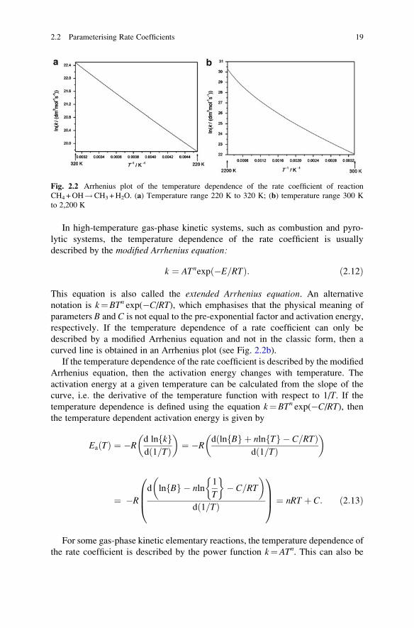
Fig. 2.2 Arrhenius plot of the temperature dependence of the rate coefficient of reaction

CH4 +OH!CH3 +H2O. (a) Temperature range 220 K to 320 K; (b) temperature range 300 K

to 2,200 K

2.2 Parameterising Rate Coefficients 19

considered as a truncated form of the extended Arrhenius equation. Another type of

unusual temperature dependence is when there are two different routes from the

reactants to the products; therefore, the temperature dependence of the reaction step

in a wide temperature range is described by the sum of two Arrhenius expressions:

k ¼ A1Tn1exp �E1=RTð Þ þ A2T

n2exp �E2=RTð Þ. An example is the case of reaction

HO2 +OH¼H2O+O2 (Burke et al. 2013).

Reaction CH4 +OH!CH3 +H2O is the major consumption reaction of methane

in the troposphere, where the typical temperature extremes are 220 K (�53 �C) and320 K (+47 �C). In this 100 K temperature range, the temperature dependence of the

rate coefficient can be described accurately with a 2-parameter Arrhenius equation

as shown in Fig. 2.2a. The same reaction is important in methane flames, where this

reaction is one of the main consuming reactions of the fuel molecules. In a methane

flame, the temperature is changing between 300 K (room temperature or laboratory

temperature) and 2,200 K, which is the typical maximum temperature of a laminar

premixed methane–air flame. When representing the temperature dependence of the

rate coefficient within this wide temperature range in an Arrhenius plot, the

obtained function is clearly curved (see Fig. 2.2b). This example shows that the

temperature dependence of the same rate coefficient can be well described by the

original Arrhenius expression within a narrow(less than 100 K) temperature range,

but only with the extended Arrhenius expression within a wide (several hundred

Kelvin) temperature range. However, the temperature dependence of some rate

coefficients can be characterised by the original Arrhenius equation within a very

wide temperature range. One example is the reaction I +H2!HI +H, where the

experimentally determined rate coefficients could be fitted using the original

Arrhenius equation over the temperature range 230 K to 2,605 K, even though

the rate coefficient changed by about 30 orders of magnitude (Michael et al. 2000).

2.2.2 Pressure Dependence of Rate Coefficients

The rate coefficients of thermal decomposition or isomerisation reactions of several

small organic molecules have been found to be pressure dependent at a given

temperature. A model reaction was the isomerisation of cyclopropane yielding

propene. The rate coefficient of the reaction was found to be first-order and pressure

independent at high pressures whilst second-order and linearly dependent on

pressure at low pressures. These types of observations were interpreted by

Lindemann et al. (1922) and Hinshelwood by assuming that the molecules of

cyclopropane (C) are colliding with any of the other molecules present in the

system (third body, denoted by M) producing rovibrationally excited cyclopropane

molecules (C*). These molecules can then isomerise (transform into another mole-

cule with the same atoms but with a different arrangement) yielding propene (P), or

further collisions may convert the excited cyclopropane molecules back to

non-excited ones: C +M⇄C* +M and C*! P. This model allowed the inter-

pretation of changing order with pressure (Pilling and Seakins 1995). Later research


confirmed that the basic idea was correct. However, it was shown that the collisions

create excited reactant species having a wide range of rovibrational energies. The

cyclopropane molecules can move up and down on an energy ladder, and the rate

coefficient of isomerisation depends on the energy of the excited reactant.

The isomerisation of cyclopropane has limited practical importance, but the

pressure-dependent decomposition or isomerisation of many molecules and radi-

cals proved to be very important in combustion and atmospheric chemistry. In these

elementary reactions, only a single species undergoes chemical transformation, and

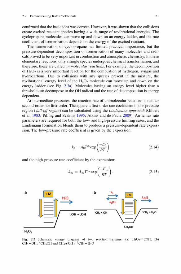
therefore, these are called unimolecular reactions. For example, the decomposition

of H2O2 is a very important reaction for the combustion of hydrogen, syngas and

hydrocarbons. Due to collisions with any species present in the mixture, the

rovibrational energy level of the H2O2 molecule can move up and down on the

energy ladder (see Fig. 2.3a). Molecules having an energy level higher than a

threshold can decompose to the OH radical and the rate of decomposition is energy

dependent.

At intermediate pressures, the reaction rate of unimolecular reactions is neither

second-order nor first-order. The apparent first-order rate coefficient in this pressure

region ( fall-off region) can be calculated using the Lindemann approach (Gilbert

et al. 1983; Pilling and Seakins 1995; Atkins and de Paula 2009). Arrhenius rate

parameters are required for both the low- and high-pressure limiting cases, and the

Lindemann formulation blends them to produce a pressure-dependent rate expres-

sion. The low-pressure rate coefficient is given by the expression:

k0 ¼ A0Tn0exp

�E0

RT

� �ð2:14Þ

and the high-pressure rate coefficient by the expression:

k1 ¼ A1Tn1exp�E1RT

� �: ð2:15Þ

Fig. 2.3 Schematic energy diagram of two reaction systems: (a) H2O2⇄ 2OH; (b)CH3 +OH⇄CH3OH and CH3+OH⇄ 1CH2 +H2O


The apparent first-order rate coefficient at any pressure can be calculated by the

expression:

k ¼ k1Pr

1þ Pr

� �F: ð2:16Þ

In the equation above, F¼ 1 in the Lindemann approach and the reduced pressure

Pr is given by

Pr ¼ k0 M½ �k1

; ð2:17Þ

where M is the third body. When calculating the effective concentration of the third

body, the collision efficiencies myi are also taken into account:

M½ � ¼Xi

myi Yi½ �: ð2:18Þ

In the case of the example reaction of H2O2 decomposition, the effective concen-

tration of the third body is calculated by Metcalfe et al. (2013) as [M]¼ 5.00[H2O]

+ 5.13[H2O2] + 0.8[O2] + 2.47[H2] + 1.87[CO] +1.07[CO2] + 0.67[Ar] + 0.43[He]+

the sum of the concentrations of all other species. Since N2 is a commonly used

bath gas within experiments, it often makes up the majority of the colliding species

concentrations. N2 is therefore assumed to have unit collision efficiency, and those of

the other species are compared against it. In the reaction H2O2(+M)⇄ 2OH (+M),

species that have similar molecular energy levels to the rovibrationally excited H2O2

molecules (like H2O2 and H2O) have large collision efficiencies, whilst noble gases

have typically small collision efficiencies. The general trend is that larger molecules

with more excitable rovibrational frequencies have larger collision efficiency factors.

There are few measurements that specifically address third-body efficiency factors,

and these values can be quite uncertain (Baulch et al. 2005). The third-body effi-

ciency factors can also be considered as temperature dependent (Baulch et al. 2005),

but even an approximate parameterisation is hindered by the lack of appropriate

experimental data. The effective third-body concentration continuously changes

during the course of a reaction according to the change of the mixture composition.

The Lindeman equation does not describe properly the pressure dependence of

the rate coefficient, and it can be improved by the application of the pressure and

temperature dependent parameter F. In the Troe formulation (Gilbert et al. 1983),

F is represented by a more complex expression:


logF ¼ logFcent 1þ logPr þ c

n� d logPr þ cð Þ� �2" #�1

; ð2:19Þ

with c¼� 0.4� 0.67 logFcent, n¼� 0.75� 1.271 logFcent, d¼ 0.14

and

Fcent ¼ 1� αð Þexp � T

T��

� �þ α exp � T

T�

� �þ exp � T��

T

� �ð2:20Þ

so that four extra parameters, α, T***, T* and T**, must be defined in order to

represent the fall-off curve with Troe parameterisation.In several cases, the pressure dependence in the fall-off region is described by

temperature-independent Fcent, but still keeping the Troe representation. For exam-

ple, for the reaction H+O2(+M)¼HO2 (+M), O Conaire et al.(2004) provided the

following Troe parameters: α¼ 0.5, T***¼ 1.0� 10�30, T*¼ 1.0� 10+30 and

T**¼ 1.0� 10+100. At combustion temperatures (T¼ 700� 2,500 K), the exponen-

tial terms are approximately exp (�1033)� 0, exp(�10�27)� exp(0)¼ 1 and exp

(�1097)� 0; therefore, using these Troe parameters in Eq. (2.20) gives a

temperature-independent Fcent¼ 0.5.

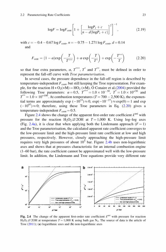
Figure 2.4 shows the change of the apparent first-order rate coefficient kuni withpressure for the reaction H2O2⇄ 2OH at T¼ 1,000 K. Using log–log axes

(Fig. 2.4a), it is clear that when applying both the Lindemann approach (F¼ 1)

and the Troe parameterisation, the calculated apparent rate coefficient converges to

the low-pressure limit and the high-pressure limit rate coefficient at low and high

pressures, respectively. However, closely approaching the high-pressure limit

requires very high pressures of about 105 bar. Figure 2.4b uses non-logarithmic

axes and shows that at pressures characteristic for an internal combustion engine

(1–60 bar), the rate coefficient cannot be approximated well with the low-pressure

limit. In addition, the Lindemann and Troe equations provide very different rate

Fig. 2.4 The change of the apparent first-order rate coefficient kuni with pressure for reaction

H2O2⇄ 2OH at temperature T¼ 1,000 K using bath gas N2. The source of data is the article of

Troe (2011); (a) logarithmic axes and (b) non-logarithmic axes


coefficients. The rate coefficient kuni corresponding to the low-pressure limit is a

linear function of pressure on both the log–log and non-logarithmic plots.

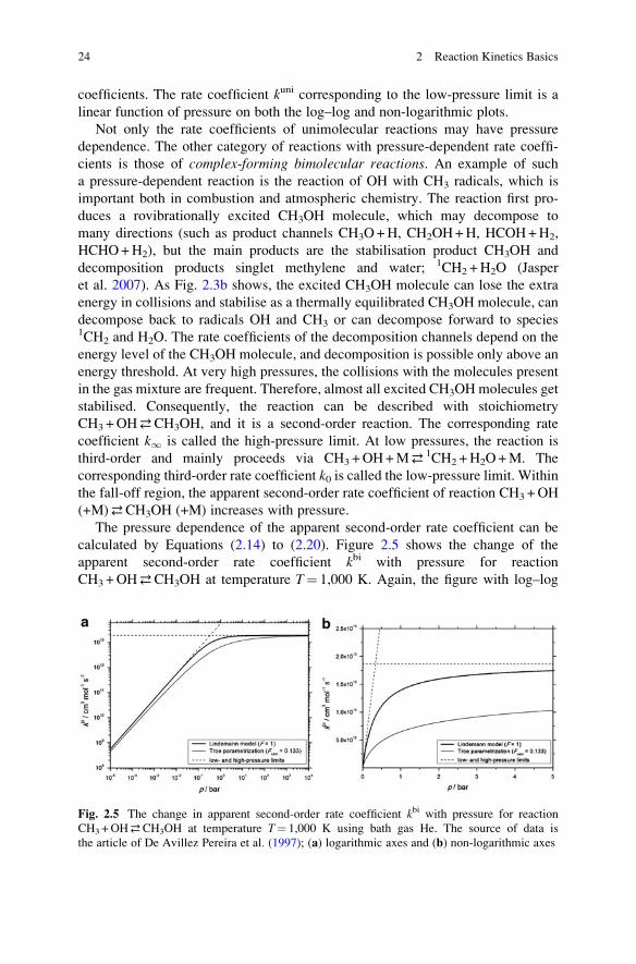
Not only the rate coefficients of unimolecular reactions may have pressure

dependence. The other category of reactions with pressure-dependent rate coeffi-

cients is those of complex-forming bimolecular reactions. An example of such

a pressure-dependent reaction is the reaction of OH with CH3 radicals, which is

important both in combustion and atmospheric chemistry. The reaction first pro-

duces a rovibrationally excited CH3OH molecule, which may decompose to

many directions (such as product channels CH3O+H, CH2OH+H, HCOH+H2,

HCHO+H2), but the main products are the stabilisation product CH3OH and

decomposition products singlet methylene and water; 1CH2 +H2O (Jasper

et al. 2007). As Fig. 2.3b shows, the excited CH3OH molecule can lose the extra

energy in collisions and stabilise as a thermally equilibrated CH3OH molecule, can

decompose back to radicals OH and CH3 or can decompose forward to species1CH2 and H2O. The rate coefficients of the decomposition channels depend on the

energy level of the CH3OH molecule, and decomposition is possible only above an

energy threshold. At very high pressures, the collisions with the molecules present

in the gas mixture are frequent. Therefore, almost all excited CH3OH molecules get

stabilised. Consequently, the reaction can be described with stoichiometry

CH3 +OH⇄CH3OH, and it is a second-order reaction. The corresponding rate

coefficient k1 is called the high-pressure limit. At low pressures, the reaction is

third-order and mainly proceeds via CH3 +OH+M⇄ 1CH2 +H2O+M. The

corresponding third-order rate coefficient k0 is called the low-pressure limit. Within

the fall-off region, the apparent second-order rate coefficient of reaction CH3 +OH

(+M)⇄CH3OH (+M) increases with pressure.

The pressure dependence of the apparent second-order rate coefficient can be

calculated by Equations (2.14) to (2.20). Figure 2.5 shows the change of the

apparent second-order rate coefficient kbi with pressure for reaction

CH3 +OH⇄CH3OH at temperature T¼ 1,000 K. Again, the figure with log–log

Fig. 2.5 The change in apparent second-order rate coefficient kbi with pressure for reaction

CH3 +OH⇄CH3OH at temperature T¼ 1,000 K using bath gas He. The source of data is

the article of De Avillez Pereira et al. (1997); (a) logarithmic axes and (b) non-logarithmic axes


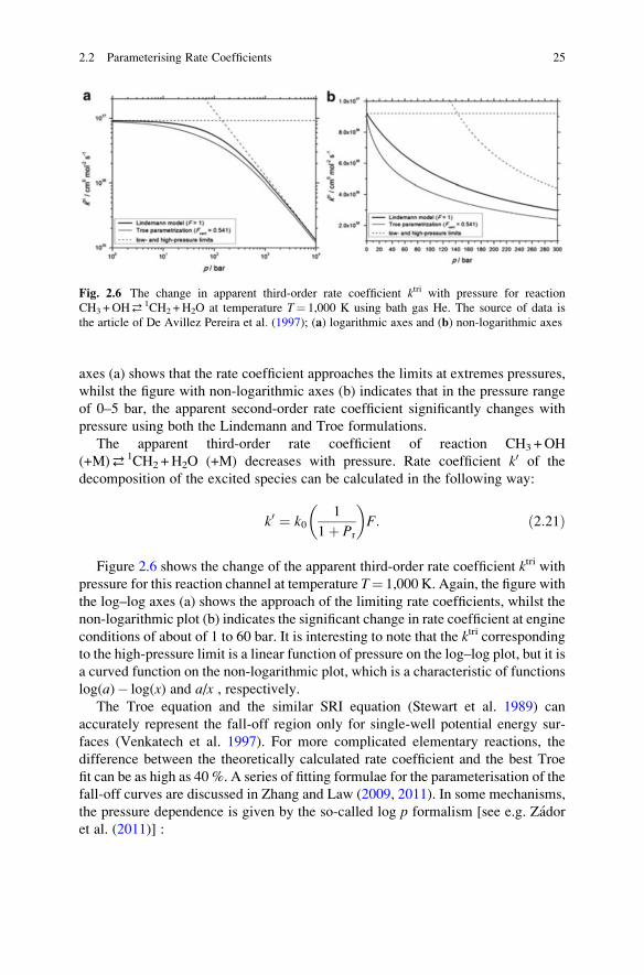
axes (a) shows that the rate coefficient approaches the limits at extremes pressures,

whilst the figure with non-logarithmic axes (b) indicates that in the pressure range

of 0–5 bar, the apparent second-order rate coefficient significantly changes with

pressure using both the Lindemann and Troe formulations.

The apparent third-order rate coefficient of reaction CH3 +OH

(+M)⇄ 1CH2 +H2O (+M) decreases with pressure. Rate coefficient k0 of the

decomposition of the excited species can be calculated in the following way:

k0 ¼ k01

1þ Pr

� �F: ð2:21Þ

Figure 2.6 shows the change of the apparent third-order rate coefficient ktri withpressure for this reaction channel at temperature T¼ 1,000 K. Again, the figure with

the log–log axes (a) shows the approach of the limiting rate coefficients, whilst the

non-logarithmic plot (b) indicates the significant change in rate coefficient at engine

conditions of about of 1 to 60 bar. It is interesting to note that the ktri correspondingto the high-pressure limit is a linear function of pressure on the log–log plot, but it is

a curved function on the non-logarithmic plot, which is a characteristic of functions

log(a)� log(x) and a/x , respectively.The Troe equation and the similar SRI equation (Stewart et al. 1989) can

accurately represent the fall-off region only for single-well potential energy sur-

faces (Venkatech et al. 1997). For more complicated elementary reactions, the

difference between the theoretically calculated rate coefficient and the best Troe

fit can be as high as 40 %. A series of fitting formulae for the parameterisation of the

fall-off curves are discussed in Zhang and Law (2009, 2011). In some mechanisms,

the pressure dependence is given by the so-called log p formalism [see e.g. Zador

et al. (2011)] :

Fig. 2.6 The change in apparent third-order rate coefficient ktri with pressure for reaction

CH3 +OH⇄ 1CH2 +H2O at temperature T¼ 1,000 K using bath gas He. The source of data is

the article of De Avillez Pereira et al. (1997); (a) logarithmic axes and (b) non-logarithmic axes


ln fkg ¼ ln fkig þ ln fkiþ1g � ln fkigð Þ ln fpg � ln fpigln fpiþ1g � ln fpig

: ð2:22Þ

Here k is the rate coefficient belonging to pressure p, whilst the ( pi, ki) pairs are aseries of tabulated rate coefficients, defined by Arrhenius parameters, belonging to

different pressures. Hence, this is an interpolation method which is linear in log p.Usually the rate coefficient at a given pressure will follow the extended Arrhenius

formulation, but this need not be the same at different pressures making the log

p formulation more flexible than the Troe formulation. Differences in third-body

efficiencies can also be accounted for each collider separately, but the log pformalism is not compatible with the effective concentration formalism [see

Eq. (2.18)]. Another possible approach is the application of Chebyshev polynomials

to represent the temperature and pressure dependencies of the apparent rate coef-

ficients (Venkatech et al. 1997). Whilst this may be more accurate in some cases

than using interpolation based on a limited number of pressures, care should be

taken not to extrapolate the use of Chebyshev polynomials outside the range in

which they were fitted. Further discussion of the handling of pressure-dependent

reactions can be found in Pilling and Seakins (1995) and Carstensen and

Dean (2007).

2.2.3 Reversible Reaction Steps

In theory, all thermal elementary reactions are reversible, which means that the

reaction products may react with each other to reform the reactants. Within the

terminology used for reaction kinetics simulations, a reaction step is called irre-

versible, either if the backward reaction is not taken into account in the simulations

or the reversible reaction is represented by a pair of opposing irreversible reaction

steps. These irreversible reactions are denoted by a single arrow “!”. Reversible

reaction steps are denoted by the two-way arrow symbol within the reaction step

expression “⇄”. In such cases, a forward rate expression may be given either in the

Arrhenius or pressure-dependent forms, and the reverse rate is calculated from the

thermodynamic properties of the species through the equilibrium constants. Hence,

if the forward rate coefficient kf i is known, the reverse rate coefficient can be

calculated from

kri ¼kf iKci

; ð2:23Þ

where Kci is the equilibrium constant expressed in molar concentrations. Kci is

obtained from the thermodynamic properties of the species.

In combustion systems, thermodynamic properties are often calculated from

14 fitted polynomial coefficients called the NASA polynomials for each species

(Burcat 1984). Seven are used for the low-temperature range Tlow to Tmid and seven


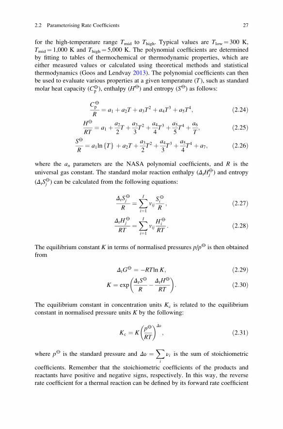
for the high-temperature range Tmid to Thigh. Typical values are Tlow¼ 300 K,

Tmid¼ 1,000 K and Thigh¼ 5,000 K. The polynomial coefficients are determined

by fitting to tables of thermochemical or thermodynamic properties, which are

either measured values or calculated using theoretical methods and statistical

thermodynamics (Goos and Lendvay 2013). The polynomial coefficients can then

be used to evaluate various properties at a given temperature (T ), such as standard

molar heat capacity (C⦵p ), enthalpy (H⦵) and entropy (S⦵) as follows:

C⦵p

R¼ a1 þ a2T þ a3T

2 þ a4T3 þ a5T

4; ð2:24ÞH⦵

RT¼ a1 þ a2

2T þ a3

3T2 þ a4

4T3 þ a5

5T4 þ a6

T; ð2:25Þ

S⦵

R¼ a1lnfTg þ a2T þ a3

2T2 þ a4

3T3 þ a5

4T4 þ a7; ð2:26Þ

where the an parameters are the NASA polynomial coefficients, and R is the

universal gas constant. The standard molar reaction enthalpy (ΔrH⦵j ) and entropy

(ΔrS⦵j ) can be calculated from the following equations:

ΔrS⦵j

R¼XIi¼1

vijS⦵i

R; ð2:27Þ

ΔrH⦵j

RT¼XIi¼1

vijH⦵

i

RT: ð2:28Þ

The equilibrium constant K in terms of normalised pressures p/p⦵ is then obtained

from

ΔrG⦵ ¼ �RTln K; ð2:29Þ

K ¼ expΔrS

⦵

R� ΔrH

⦵

RT

� �: ð2:30Þ

The equilibrium constant in concentration units Kc is related to the equilibrium

constant in normalised pressure units K by the following:

Kc ¼ Kp⦵

RT

� �Δν

; ð2:31Þ

where p⦵ is the standard pressure and Δν ¼Xi

νi is the sum of stoichiometric

coefficients. Remember that the stoichiometric coefficients of the products and

reactants have positive and negative signs, respectively. In this way, the reverse

rate coefficient for a thermal reaction can be defined by its forward rate coefficient


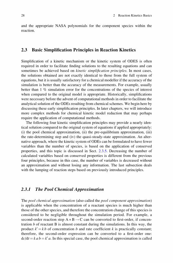
and the appropriate NASA polynomials for the component species within the

reaction.

2.3 Basic Simplification Principles in Reaction Kinetics

Simplification of a kinetic mechanism or the kinetic system of ODES is often

required in order to facilitate finding solutions to the resulting equations and can

sometimes be achieved based on kinetic simplification principles. In most cases,

the solutions obtained are not exactly identical to those from the full system of

equations, but it is usually satisfactory for a chemical modeller if the accuracy of the

simulation is better than the accuracy of the measurements. For example, usually

better than 1 % simulation error for the concentrations of the species of interest

when compared to the original model is appropriate. Historically, simplifications

were necessary before the advent of computational methods in order to facilitate the

analytical solution of the ODEs resulting from chemical schemes. We begin here by

discussing these early simplification principles. In later chapters, we will introduce

more complex methods for chemical kinetic model reduction that may perhaps

require the application of computational methods.

The following four kinetic simplification principles may provide a nearly iden-

tical solution compared to the original system of equations if applied appropriately:

(i) the pool chemical approximation, (ii) the pre-equilibrium approximation, (iii)

the rate-determining step and (iv) the quasi-steady-state approximation. An alter-

native approach, where the kinetic system of ODEs can be formulated to have fewer

variables than the number of species, is based on the application of conserved

properties, and this topic is discussed in Sect. 2.3.5. Decreasing the number of

calculated variables based on conserved properties is different from the previous

four principles, because in this case, the number of variables is decreased without

an approximation and without losing any information. The last subsection deals

with the lumping of reaction steps based on previously introduced principles.

2.3.1 The Pool Chemical Approximation

The pool chemical approximation (also called the pool component approximation)is applicable when the concentration of a reactant species is much higher than

those of the other species, and therefore the concentration change of this species is

considered to be negligible throughout the simulation period. For example, a

second-order reaction step A +B!C can be converted to first-order, if concen-

tration b of reactant B is almost constant during the simulations. In this way, the

product k0 ¼ k b of concentration b and rate coefficient k is practically constant;

therefore, the second-order expression can be converted to a first-order one:

dc/dt¼ k a b¼ k0 a. In this special case, the pool chemical approximation is called


the pseudo-first-order approximation and k0 is the pseudo-first-order rate

coefficient.

2.3.2 The Pre-equilibrium Approximation

The pre-equilibrium approximation (PEA; also called the partial equilibriumapproximation or fast–equilibrium approximation) is applicable when the species

participating in a pair of fast-equilibrium reactions are consumed by slow reactions.

After the onset of an equilibrium, the rates of the forward and backward reactionsbecome equal to each other, and therefore the ratios of the concentrations of the

participating species can be calculated from the stoichiometry of the reaction steps

and the equilibrium constant. According to the pre-equilibrium approximation, if

the rates of the equilibrium reactions are much higher than the rates of the other

reactions consuming the species participating in the equilibrium reactions, then the

concentrations of these species are determined, with good approximation, by the

equilibrium reactions only.

As an example, let us consider the equilibrium reaction A⇄B. The

corresponding rate coefficients are k1 and k2, and the equilibrium constant is

denoted by K¼ k1/k2. In the case of an onset of equilibrium, the rates of the

opposing reactions are identical: k1a¼ k2b, and therefore, b¼ k1/k2a¼Ka. Nowconsider the reaction system A ⇄ B!C, where species B is consumed by a slow

reaction with a small rate coefficient k3 compared to k1 and k2. In this case, we can

still assume that b¼Ka is a good approximation, and thus, dc/dt¼ k3 b, dc/dt¼ k3Ka. Therefore, the concentration of B is not required in order to calculate

the rate of production of C as long as the rate coefficients are known.

A common example of such a situation is the enzyme-substrate reaction

involved in biochemical pathways. In this type of reaction, an enzyme E binds to

a substrate S to produce an enzyme-substrate intermediate ES, which then forms the

final product P:

Eþ S ⇄k1

k�1

ES!k2 Eþ P:

Here the rate of production of the final product (usually an essential biomolecule)

can be derived using the pre-equilibrium approximation to be

d P½ �dt

¼ k2k1k�1

E½ � S½ � ¼ k2K E½ � S½ �;

where the square brackets indicate the molar concentrations of the given species.

Another common situation is when a large organic molecule isomerises in a

fast–equilibrium reaction to a low-concentration, more reactive form, and this more

reactive species is consumed by a slow reaction. Using the equation dc/dt¼ k3Kameans that the rate equation contains the less reactive organic species that is present

in higher concentration and therefore can be measured more easily.

2.3 Basic Simplification Principles in Reaction Kinetics 29

2.3.3 Rate-Determining Step

Even in the case of large reaction mechanisms, the production rate of a reactant or

final product of the overall chemical reaction may depend mainly on the rate

coefficient of a single reaction step. This reaction step is called the rate-determiningstep. If we have sequential first-order reactions, then the reaction step having the

smallest rate coefficient is the rate-determining one. In this case, the production rate

of the final product is equal to the rate coefficient of the rate-determining step

multiplied by the concentration of the reactant of this reaction step. In this example

if k2 k1, k3, k4, k5, then dp/dt� k2b.In the case of an arbitrary mechanism, the rate-determining step is characterised

by the fact that increasing its rate coefficient increases the production rate of the

product significantly. However, in general, this may not be the reaction step having

the smallest rate coefficient. For example, when species P is produced from species

A in parallel pathways, then the rate coefficient of the rate-determining step may be

relatively high. In the example below, rate coefficient k1 belonging to the rate-

determining step is relatively large if k3, k4 k1 k2:

In the general case, we have to investigate how a small change of rate coefficient

kj changes the production rate d yi/d t of product Yi. This effect appears in the local

rate sensitivity coefficient ∂(dci/dt)/∂kj (see Sect. 5.2). If this coefficient is much

higher for reaction j than for the other reaction steps, then reaction j is the rate-

determining step of the production of species i (Turanyi 1990).

2.3.4 The Quasi-Steady-State Approximation (QSSA)

The quasi-steady-state approximation (QSSA) is also called the Bodenstein prin-

ciple, after one of its first users (Bodenstein 1913). As a first step, species are

selected that will be called quasi-steady-state (or QSS) species. The QSS-species

are usually highly reactive and low-concentration intermediates, like radicals. The

production rates of these species are set to zero in the kinetic system of ODEs. The

corresponding right-hand sides form a system of algebraic equations. These



algebraic equations can be used to calculate the concentrations of the QSS-species

from the concentrations of the other (non-QSS) species. The system of ODEs for

the non-QSS-species and the system of algebraic equations for the QSS-species

together form a coupled system of differential algebraic equations. For the success-

ful application of the QSSA, the solution of this coupled system of differential

algebraic equations should be very close to those of the original system of kinetic

ODEs. In some cases, the system of algebraic equations can be solved separately,

that is, the concentrations of all QSS-species can be calculated from (explicit)

algebraic equations. The calculated QSS-species concentrations can then be used

in the system of kinetic ODEs for the remaining species. In this case, following the

application of the QSSA, the kinetic system of ODEs is transformed to a smaller

system of ODEs having fewer variables. The background to the QSSA is that in

chemical kinetic models, the timescales involved usually span quite a wide range

(see Sect. 6.2).

As an example, consider the following reaction sequence where B is a

QSS-species linking reactant A to product C:

A ⇄k1

k�1

B !k2 C:

If the QSSA is applied to B, then we assume:

d B½ �dt

¼ 0 ð2:32Þ

so that

k1 A½ � � k�1 B½ � � k2 B½ � ¼ 0: ð2:33Þ

Therefore,

B½ � ¼ k1k�1 þ k2

A½ �: ð2:34Þ

Hence,

d C½ �dt

¼ k2 B½ � ¼ k1k2 A½ �k�1 þ k2

¼ k0A½ �; ð2:35Þ

where

k0 ¼ k1k2

k�1 þ k2: ð2:36Þ

Therefore, the above set of reactions can be replaced by a single reaction of the

form:



A ! C ð2:37Þ

with the effective rate coefficient k’ defined in Eq. (2.36). The quantitative kinetic

involvement of intermediate B in the overall reaction is encapsulated in k0, but thespecies has been removed from the mechanism. Should the concentration of B be

required, it can be calculated from the expression (2.34), but usually the concen-

trations of the QSS-species are not required in practical applications. Therefore, the

method constitutes their complete removal from the scheme, thus reducing the

overall number of variables in the model and also usually its stiffness since the

range of timescales remaining has been reduced .

Whilst it is quite straightforward to comprehend the applicability of the previous

three basic kinetic simplification principles, the QSSA is not so easy to understand.

For example, it may seem strange that the solution of a coupled system of algebraic

differential equations can be very close to the system of ODEs. Another surprising

feature is that the concentrations of QSS-species can vary substantially over time;

for example, the QSSA has found application in oscillating systems (Tomlin

et al. 1992). The key to the success of the QSSA is the proper selection of the

QSS-species based on the error induced by its application. The interpretation of the

QSSA and the error induced by the application of this approximation will be

discussed fully in Sect. 7.8.

2.3.5 Conserved Properties

As noted above, the consideration of conserved properties allows the kinetic system

of ODEs to contain fewer variables than the number of species. However, it is an

exact transformation, and therefore it is usually handled separately from the rules

above which are based on approximations.

In many reaction mechanisms, there are conserved properties. The simplest

conserved property occurs when the sum of the molar concentrations is constant.

This is obtained when the volume is constant and for each reaction step

0 ¼Xj

ν Jij � νB

ij , that is, the change of the number of moles is zero for each

reaction step.

In a closed chemical system, the chemical reactions do not change the moles of

elements, and therefore the number of moles of each element is a conserved

property. Other conserved properties include the total enthalpy in an adiabatic

system or the charge in an electrochemical system. Another way of referring to a

conserved property is as a reaction invariant (Gadewar et al. 2001). If an atomic

group remains unchanged during the reaction steps, then its number of moles is also

a conserved property (conserved moiety). Such a conserved moiety may be, for

example, the adenosine group, and the sum of species AMP, ADP and ATP may

remain constant in a closed biochemical system (Vallabhajosyula et al. 2006).



The presence of conserved elements and conserved moieties cause linear depen-

dence between the rows of the stoichiometric matrix ν and decrease the rank of the

stoichiometric matrix. In most cases, the number of species NS is much less than the

number of reaction steps NR, that is, NS<NR. If the stoichiometric matrix ν has NR

rows and NS columns, and conserved properties are not present, then the rank of the

stoichiometric matrix is usually NS. If NC conserved properties are present, then the

rank of the stoichiometric matrix is N¼NS�NC. In this case, the original system of

ODEs can be replaced by a system of ODEs having N variables, since the other

concentrations can be calculated from the computed concentrations using algebraic

relations related to the conserved properties.

2.3.6 Lumping of Reaction Steps

In some cases, without much mathematical background, common sense rules can be

applied to the simplification of reaction mechanisms by lumping the reaction steps.

For example, reaction steps having common reactants can be lumped together:

A þ B ! C þ D 0:4kA þ B ! E þ F 0:6k

Such reactions are common in detailed mechanisms. The usual terminology is that

reaction “A +B! products” is a multichannel reaction that has two reactionchannels, one resulting in products C +D and the other products E + F. The overall

rate coefficient of the reaction is therefore k, whilst the channel ratio is 0.4:0.6. A

synonym of the term channel ratio is the branching ratio. Following the rules for

the creation of the kinetic system of differential equations, the two chemical

equations above result in exactly the same terms when starting from the single

chemical equation below:

A þ B ! 0:4 C þ 0:4 D þ 0:6 E þ 0:6 F k

The number of reaction steps in the mechanism is decreased by one, but since

lumping of the reaction steps resulted in exactly the same set of ODEs, there is no

gain in simulation speed. Nevertheless, the lumping of multichannel reactions as

above is common in atmospheric chemical mechanisms, because it may clarify the

main reaction routes for the user.

Reaction steps can also be lumped using the principle of a rate-determining step

(see Sect. 2.3.3). Let us consider the following two reactions:

A þ B ! C þ D r1 ¼ k1ab slow

D þ E ! F r2 ¼ k2de fast:

The first, slow reaction, is the rate-determining step, and therefore, the rate of the

lumped reaction obtained by merging these two reactions can be calculated by the


equation r¼ k1ab. If we want to keep the mass action kinetics formalism, then on

the left-hand side of the lumped reaction should be A+B. During the course of

these two reactions, A, B and E are consumed; C and F are produced. Equal

amounts of D are consumed and produced; therefore, D should not be present in

the lumped equation. Species E is consumed, but since it is not part of the rate-

determining step, it should not be present on the left-hand side of the chemical

equation. Therefore, it appears on the right-hand side, with a �1 stoichiometric

coefficient. The lumped reaction is the following:

A þ B ! C þ F� E r ¼ k1ab:

Using the rules of mass action kinetics, (almost) the same equations can be derived

for the production rates of all species but D. The presence of a negative stoichio-

metric coefficient is perhaps surprising at first glance, but there are several lumped

atmospheric chemical mechanisms (Gery et al. 1989) that contain negative stoichio-

metric coefficients on the right-hand side of some chemical equations.

One result of the reaction lumping above is the removal of the highly reactive

species D. This means that a fast timescale was removed from the system, and the

stiffness of the corresponding ODE system was decreased. The calculation of

lifetimes of species is discussed in Sect. 6.2. Reaction lumping based on timescales

may remove species and decrease stiffness, and thus may lead to increases in

simulation speed. For example, its application was successful for the further

reduction of a skeletal scheme describing n-heptane oxidation in Peters

et al. (2002). This will be discussed more fully in connection with the application

of the QSSA in Sect. 7.8.6.

References

Aranyi, P., Toth, J.: A full stochastic description of the Michaelis–Menten reaction for small

systems. Acta Biochim. Biophys. Acad. Sci. Hung. 12, 375–388 (1977)

Atkins, P., de Paula, J.: Atkins’ Physical Chemistry, 9th edn. Oxford University Press, Oxford

(2009)

Bamford, C.H., Tipper, C.F.H., Compton, R.G. (eds.): Theory of Kinetics. Elsevier, Amsterdam

(1969)

Baulch, D.L., Bowman, C.T., Cobos, C.J., Cox, R.A., Just, T., Kerr, J.A., Pilling, M.J., Stocker, D.,

Troe, J., Tsang, W., Walker, R.W., Warnatz, J.: Evaluated kinetic data for combustion

modeling: Supplement II. J. Phys. Chem. Ref. Data 34, 757–1397 (2005)

Belousov, B.P.: Периодически действующая реакция и ее механизм. Сборник рефератов порадиационной медицине 147, 145 (1959)

Belousov, B.P.: A periodic reaction and its mechanism. In: Field, R.J., Burger, M. (eds.) Oscilla-

tions and Traveling Waves in Chemical Systems. Wiley, New York (1985)

Bodenstein, M.: Eine Theorie der photochemischen Reaktionsgeschwindigkeiten. Z. Phys. Chem.

85, 329–397 (1913)




Bunker, D.L., Garrett, B., Kliendienst, T., Long III, G.S.: Discrete simulation methods in com-

bustion kinetics. Combust. Flame 23, 373–379 (1974)

Burcat, A.: Thermochemical Data for Combustion Calculations. Springer, New York (1984)

Burke, M., Chaos, M., Ju, Y., Dryer, F.L., Klippenstein, S.: Comprehensive H2/O2 kinetic model

for high-pressure combustion. Int. J. Chem. Kinet. 44, 444–474 (2012)

Burke, M.P., Klippenstein, S.J., Harding, L.B.: A quantitative explanation for the apparent

anomalous temperature dependence of OH + HO2 ¼ H2O + O2 through multi-scale modeling.

Proc. Combust. Inst. 34, 547–555 (2013)

Carstensen, H.H., Dean, A.M.: The kinetics of pressure-dependent reactions. In: Carr, R.W. (ed.)

Modeling of Chemical Reactions, vol. 42, pp. 105–187. Amsterdam, Elsevier (2007)

De Avillez Pereira, R., Baulch, D., Pilling, M.J., Robertson, S.H., Zeng, G.: Temperature and

pressure dependence of the multichannel rate coefficients for the CH3 + OH system. J. Phys.

Chem. A 101, 9681–9693 (1997)

Drake, G.W.F. (ed.): Springer Handbook of Atomic, Molecular, and Optical Physics. Springer,

Berlin (2005)

Erdi, P., Lente, G.: Stochastic Chemical Kinetics: Theory and (Mostly) Systems Biological

Applications. Springer, Heidelberg (2014)

Erdi, P., Toth, J.: A kemiai reakcio termodinamikajanak sztochasztikus formulazasarol (On the

stochiastic formulation of the thermodynamics of chemical reactions). A kemia ujabb

eredmenyei, vol. 41. Akademiai Kiado, Budapest (1976)

Erdi, P., Toth, J.: Mathematical Models of Chemical Reactions. Princeton University Press,

Princeton (1989)

Erdi, P., Sipos, T., Toth, J.: Osszetett kemiai reakciok sztochasztikus szimulalasa szamıtogeppel

(Stochiastic simulation of complex chemical reactions using computer). Magyar Kemiai

Folyoirat 79, 97–108 (1973)

Field, R.J., Noyes, R.M.: Oscillations in chemical systems. IV. Limit cycle behavior in a model of

a real reaction. J. Chem. Phys. 60, 1877–1884 (1974)

Field, R.J., Koros, E., Noyes, R.M.: Oscillations in chemical systems II. Thorough analysis of

temporal oscillation in the bromate-cerium-malonic acid system. J. Am. Chem. Soc. 94, 8649–8664 (1972)

Gadewar, S.B., Doherty, M.F., Malone, M.F.: A systematic method for reaction invariants and

mole balances for complex chemistries. Comput. Chem. Eng. 25, 1199–1217 (2001)

Gery, M.W., Whitten, G.Z., Killus, J.P., Dodge, M.C.: A photochemical kinetics mechanism for

urban and regional scale computer modeling. J. Geophys. Res. D94, 12925–12956 (1989)

Gilbert, R.G., Luther, K., Troe, J.: Theory of thermal unimolecular reactions in the fall-off range.

II. Weak collision rate constants. Berichte Bunsenges. Phys. Chem. 87, 169–177 (1983)

Gillespie, D.T.: A general method for numerically simulating the stochastic time evolution of

coupled chemical reactions. J. Comput. Phys. 22, 403–434 (1976)

Gillespie, D.T.: Exact stochastic simulation of coupled chemical reactions. J. Phys. Chem. 81,2340–2361 (1977)

Gillespie, D.T.: Stochastic simulation of chemical kinetics. Annu. Rev. Phys. Chem. 58, 35–55(2007)

Goos, E., Lendvay, G.: Calculation of molecular thermochemical data and their availability in

databases. In: Battin-Leclerc, F., Simmie, J.M., Blurock, E. (eds.) Cleaner Combustion:

Developing Detailed Chemical Kinetic Models, pp. 515–547. Springer, London (2013)

Hong, Z., Davidson, D.F., Hanson, R.K.: An improved H2/O2 mechanism based on recent shock

tube/laser absorption measurements. Combust. Flame 158, 633–644 (2011)

Jasper, A.W., Klippenstein, S.J., Harding, L.B., Ruscic, B.: Kinetics of the reaction of methyl

radical with hydroxyl radical and methanol decomposition. J. Phys. Chem. A 111, 3932–3950(2007)

Konnov, A.A.: Remaining uncertainties in the kinetic mechanism of hydrogen combustion.

Combust. Flame 152, 507–528 (2008)

References 35

Kraft, M., Wagner, W.: An improved stochastic algorithm for temperature-dependent homoge-

neous gas phase reactions. J. Comput. Phys. 185, 139–157 (2003)

Kurtz, T.G.: The relationship between stochastic and deterministic models of chemical reactions.

J. Chem. Phys. 57, 2976–2978 (1972)

Li, H., Cao, Y., Petzold, L.R., Gillespie, D.T.: Algorithms and software for stochastic simulation

of biochemical reacting systems. Biotechnol. Prog. 24, 56–61 (2008)

Lindemann, F.A., Arrhenius, S., Langmuir, I., Dhar, N.R., Perrin, J., McC. Lewis, W.C.: Discus-

sion on “the radiation theory of chemical action”. Trans. Faraday Soc. 17, 598–606 (1922)

Metcalfe, W.K., Burke, S.M., Ahmed, S.S., Curran, H.J.: A hierarchical and comparative kinetic

modeling study of C1�C2 hydrocarbon and oxygenated fuels. Int. J. Chem. Kinet. 45, 638–675(2013)

Michael, J.V., Kumaran, S.S., Su, M.C., Lim, K.P.: Thermal rate constants over thirty orders of

magnitude for the I + H2 reaction. Chem. Phys. Lett. 319, 99–106 (2000)

O Conaire, M.O., Curran, H.J., Simmie, J.M., Pitz, W.J., Westbrook, C.K.: A comprehensive

modeling study of hydrogen oxidation. Int. J. Chem. Kinet. 36, 603–622 (2004)

Peters, N., Paczko, G., Seiser, R., Seshadri, K.: Temperature cross-over and non-thermal runaway

at two-stage ignition of n-heptane. Combust. Flame 128, 38–59 (2002)

Pilling, M.J., Seakins, P.W.: Reaction Kinetics. Oxford University Press, Oxford (1995)

Raj, G.: Chemical Kinetics. Krishna Prakashan Media P Ltd, Meerut (2010)

Rodiguin, N.M., Rodiguina, E.N.: Consecutive Chemical Reactions. Mathematical Analysis and

Development. D. van Nostrand, Princeton (1964)

Scott, S.K.: Chemical Chaos. International Series of Monographs on Chemistry, vol. 24.

Clarendon Press, Oxford (1990)

Stewart, P.H., Larson, C.W., Golden, D.M.: Pressure and temperature dependence of reactions

proceeding via a bound complex. 2. Application to 2CH3 ! C2H5 + H. Combust. Flame 75,25–31 (1989)

Szabo, Z.G.: Kinetic characterization of complex reaction systems. In: Bamford, C.H., Tipper,

C.F.H. (eds.) Comprehensive Chemical Kinetics, vol. 2, pp. 1–80. Amsterdam, Elsevier (1969)

Tomlin, A.S., Pilling, M.J., Turanyi, T., Merkin, J.H., Brindley, J.: Mechanism reduction for the

oscillatory oxidation of hydrogen: sensitivity and quasi-steady-state analyses. Combust. Flame

91, 107–130 (1992)

Tomlin, A.S., Li, G.Y., Rabitz, H., Toth, J.: A general-analysis of approximate nonlinear lumping

in chemical-kinetics 2. Constrained lumping. J. Chem. Phys. 101, 1188–1201 (1994)

Toth, J., Erdi, P.: A formalis reakciokinetika modelljei, problemai es alkalmazasai (The models,

problems and applications of formal reaction kinetics). A kemia ujabb eredmenyei, vol. 41.

Akademiai Kiado, Budapest (1978)

Troe, J.: The thermal dissociation/recombination reaction of hydrogen peroxide H2O2(+M)¼2OH

(+M) III. Analysis and representation of the temperature and pressure dependence over wide

ranges. Combust. Flame 158, 594–601 (2011)

Turanyi, T.: Sensitivity analysis of complex kinetic systems.Tools and applications. J. Math.

Chem. 5, 203–248 (1990)

Turanyi, T., Gyorgyi, L., Field, R.J.: Analysis and simplification of the GTF model of the

Belousov-Zhabotinsky reaction. J. Phys. Chem. 97, 1931–1941 (1993)

Vallabhajosyula, R.R., Chickarmane, V., Sauro, H.M.: Conservation analysis of large biochemical

networks. Bioinformatics 22, 346–353 (2006)

Varga, T., Nagy, T., Olm, C., Zsely, I.G., Palvolgyi, R., Valko, E., Vincze, G., Cserhati, M.,

Curran, H.J., Turanyi, T.: Optimization of a hydrogen combustion mechanism using both direct

and indirect measurements. Proc. Combust. Inst. (2015, in press) http://dx.doi.org/10.1016/

j.proci.2014.06.071

Venkatech, P.K., Chang, A.Y., Dean, A.M., Cohen, M.H., Carr, R.W.: Parameterization of

pressure- and temperature-dependent kinetics in multiple well reactions. AIChE J. 43, 1331–1340 (1997)


http://dx.doi.org/10.1016/j.proci.2014.06.071


Waage, P., Guldberg, C.M.: Studies concerning affinity. Forhandlinger: Videnskabs-Selskabet i

Christiana 35 (1864)

Warnatz, J., Maas, U., Dibble, R.W.: Combustion. Physical and Chemical Fundamentals, Model-

ing and Simulation, Experiments, Pollutant Formation, 4th edn. Springer, Berlin (2006)

Zador, J., Taatjes, C.A., Fernandes, R.X.: Kinetics of elementary reactions in autoignition chem-

istry. Prog. Energy Combust. Sci. 37, 371 (2011)

Zhabotinsky, A.M.: Периодический процесс окисления малоновой кислоты растворе(исследование кинетики реакции Белоусова). Биофизика 9, 306–311 (1964)

Zhang, P., Law, C.K.: A fitting formula for the falloff curves of unimolecular reactions. Int.

J. Chem. Kinet. 41, 727–734 (2009)

Zhang, P., Law, C.K.: A fitting formula for the falloff curves of unimolecular reactions. II:

Tunneling effects. Int. J. Chem. Kinet. 43, 31–42 (2011)

References 37

Chapter 3

Mechanism Construction and the Sources

of Data

Abstract The creation of a kinetic reaction mechanism involves the definition of

stoichiometries for each of the reaction steps and also the provision of values for all

kinetic and thermodynamic parameters. Whilst this sounds like a simple task, in

reality, it is extremely complicated. Reaction mechanisms often undergo updates

and revisions over time, as the quantification of input parameters is improved

through new kinetic studies or as new reaction steps are identified as being

important. Recently developed mechanisms describing a range of kinetic problems

in combustion, pyrolysis, atmospheric chemistry and biochemistry tend to be very

large, and it is almost impossible to generate such mechanisms by hand. Fortu-

nately, several mathematical methods and computational tools have been elabo-

rated for the automatic generation of reaction mechanisms in each of these fields.

These computer codes are able to handle various sources of chemical kinetic and

thermodynamic data and will be described in this chapter. We also describe the

variety of data sources which are used to help quantify the parameters within

developed mechanisms.

3.1 Automatic Mechanism Generation

Historically many chemical kinetic mechanisms have been the result of extensive

and careful development work by teams of experts in particular fields. The manual

generation of mechanisms begins with the selection of important species, which

usually include not just reactants and products but also important intermediates that

are necessary in order to predict the production rates of the key products or other

key quantities, for example, ignition behaviour or dynamic features such as oscil-

lations. The types of reactions that can occur between these coupled groups of

species must then be specified along with appropriate thermochemical data. Over

time, the development of expertise has meant that protocols can be specified for

different types of application which indicate the reaction classes that each category

of important species can undergo. Typically, even at the mechanism construction

stage, certain reaction classes are ignored if their rates are very slow compared to

the overall timescales of interest, they are too endothermic or they are too complex



39

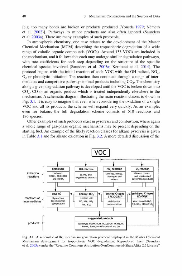
[e.g. too many bonds are broken or products produced (Yoneda 1979; Nemeth

et al. 2002)]. Pathways to minor products are also often ignored (Saunders

et al. 2003a). There are many examples of such protocols.

In atmospheric chemistry, one case relates to the development of the Master

Chemical Mechanism (MCM) describing the tropospheric degradation of a wide

range of volatile organic compounds (VOCs). Around 135 VOCs are included in

the mechanism, and it follows that each may undergo similar degradation pathways,

with rate coefficients for each step depending on the structure of the specific

chemical species involved (Saunders et al. 2003a; Kerdouci et al. 2014). The

protocol begins with the initial reaction of each VOC with the OH radical, NO3,

O3 or photolytic initiation. The reaction then continues through a range of inter-

mediates and competitive pathways to final products including CO2. The chemistry

along a given degradation pathway is developed until the VOC is broken down into

CO2, CO or an organic product which is treated independently elsewhere in the

mechanism. A schematic diagram illustrating the main reaction classes is shown in

Fig. 3.1. It is easy to imagine that even when considering the oxidation of a single

VOC and all its products, the scheme will expand very quickly. As an example,

even for butane, the full degradation scheme consists of 510 reactions and

186 species.

Other examples of such protocols exist in pyrolysis and combustion, where again

a whole range of gas-phase organic mechanisms may be present depending on the

starting fuel. An example of the likely reaction classes for alkane pyrolysis is given

in Table 3.1 and for alkane oxidation in Fig. 3.2. A more detailed discussion of the

Fig. 3.1 A schematic of the mechanism generation protocol employed in the Master Chemical

Mechanism development for tropospheric VOC degradation. Reproduced from (Saunders

et al. 2003a) under the “Creative Commons Attribution-NonCommercial-ShareAlike 2.5 License”

40 3 Mechanism Construction and the Sources of Data

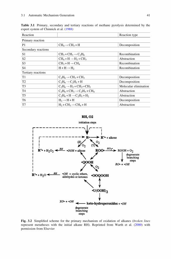
Table 3.1 Primary, secondary and tertiary reactions of methane pyrolysis determined by the

expert system of Chinnick et al. (1988)

Reaction Reaction type

Primary reaction

P1 CH4!CH3 +H Decomposition

Secondary reactions

S1 CH3 +CH3!C2H6 Recombination

S2 CH4 +H!H2 +CH3 Abstraction

S3 CH3 +H!CH4 Recombination

S4 H+H!H2 Recombination

Tertiary reactions

T1 C2H6!CH3 +CH3 Decomposition

T2 C2H6!C2H5 +H Decomposition

T3 C2H6!H2 +CH2¼CH2 Molecular elimination

T4 C2H6 +CH3!C2H5 +CH4 Abstraction

T5 C2H6 +H!C2H5 +H2 Abstraction

T6 H2!H+H Decomposition

T7 H2 +CH3!CH4 +H Abstraction

Fig. 3.2 Simplified scheme for the primary mechanism of oxidation of alkanes (broken linesrepresent metatheses with the initial alkane RH). Reprinted from Warth et al. (2000) with

permission from Elsevier

3.1 Automatic Mechanism Generation 41

reaction classes used to describe the oxidation of a range of fuel types is given in

Chaps. 2 and 3 of Battin-Leclerc et al. (2013).

It becomes immediately clear that as the reactants become more abundant

(e.g. in the case of tropospheric chemistry) or the starting fuels more complex

(in the case of pyrolysis and combustion), then the manual construction of mech-

anisms becomes a daunting task, even where protocols describing key reaction

classes exist. For this reason, attempts have been made by different research groups

to utilise the expert knowledge available from such protocols within computer

codes for the construction of reaction mechanisms. This is still a challenging

problem since for a reaction generator to produce a viable set of elementary

reactions, it should consider reactions between all combinations of species but

never produce the same reaction twice. Such methods must also avoid the possible

combinatorial explosion that may exist if all reaction possibilities are considered.

The protocols describing viable reaction classes introduced above have a role to

play here, since unlikely reaction classes must be excluded at this stage to avoid the

mechanism becoming uncontrollably large. It may also be possible to lump together

similar species types that undergo the same reaction pathways at the mechanism

generation stage in order to limit the size of the final mechanism (Bounaceur

et al. 1996; Ranzi et al. 1995, 2001). Species lumping will be described in more

detail in Sect. 7.7 . The application of the QSSA has also been tested within the

mechanism generation context by the RMG code developed at MIT (Van Geem

et al. 2006; Green et al. 2013) . The RMG code (Green et al. 2001) was successfully

applied for the generation of detailed mechanisms for the combustion of several

butanol isomers (Van Geem et al. 2010; Hansen et al. 2011, 2013; Harper

et al. 2011) and other chemical systems (Matheu et al. 2003; Jalan et al. 2013).

Examples of such expert systems for kinetic reaction mechanism generation are

available in many fields of application of kinetic modelling. In pyrolysis and

combustion, an early example was developed by Chinnick et al. (1988) based on

logical programming. The program was used to develop detailed schemes for the

pyrolysis of C1–C4 hydrocarbons, and in general, the schemes compared well with

those proposed by human experts. A similar approach was also undertaken by

Chevalier et al. (1990) in Stuttgart for the oxidation of higher hydrocarbons. This

program also incorporated rate coefficient data for known reactions from kinetic

data evaluations with extensions to unknown reactions based on reaction type and

species structure, using simple rules such as those described by Atkinson (Atkinson

1986, 1987; Kwok and Atkinson 1995) for rate coefficients in tropospheric chemistry.

An extension to these types of methodologies was developed in Milan as part of

the MAMOX code (Ranzi et al. 1995, 2005). Here automatic simplification of the

mechanism is incorporated into the generation procedure by considering species

isomers with similar kinetic behaviour as a single lumped species (Ranzi

et al. 2001). By also lumping parallel reaction pathways for these similar isomers

and fitting lumped reaction rates to predictions from the full scheme, large reductions

in the size of the generated mechanism can be achieved. The obvious advantage here

is in the lower computational requirements of the generated mechanism.


http://dx.doi.org/10.1007/978-3-662-44562-4_2

http://dx.doi.org/10.1007/978-3-662-44562-4_3


Other examples in combustion include REACTION developed by Blurock

(1995, 2004a; reaction\analysis; Blurock 2004b, c; Moreac et al. 2006; Mersin

et al. 2014) and EXGAS, first introduced by Come et al. and continuously further

developed by subsequent researchers in Nancy (Warth et al. 2000; Glaude

et al. 2000; Battin-Leclerc et al. 2000, 2008). Actually the EXGAS system is part

of a comprehensive modelling system which also includes a kinetic data base and

programs for the estimation of thermochemical parameters (Muller et al. 1995).

Over time these types of programs have become more sophisticated and are now

able to deal with wider classes of fuels than simple alkanes. Recent applications, for

example, have extended to heavy alkanes (Ranzi et al. 2005, 2004; Buda et al. 2005;

Biet et al. 2008), oxygenated species (Glaude et al. 2010; Hakka et al. 2010) and

biomass fuels (Rangarajan et al. 2010), and aqueous phase oxidation (Li and

Crittenden 2009). A review of the principles involved and the features of the

different systems is provided in Pierucci and Ranzi (2008). Liu et al. (2012)

developed an n-decane combustion mechanism using the automating generation

program ReaxGen and generated various skeletal mechanisms using the Directed

Relation Graph (DRG) method (see Sect. 7.5).

Matheu and Grenda (2005a, b) applied the mechanism generation tool

XMG-PDep (Grenda et al. 2003; Matheu et al. 2003) to high-conversion,

pyrocarbon-depositing ethane pyrolysis. The code generated the reaction pathways

governing the observed minor products acetylene, propylene, 1,3-butadiene and

benzene. They also investigated the effects of large groups of radical dispropor-

tionation reactions, omitted reaction families, and the possibility that pressure

changes in the reactor could alter the distribution of the deposition precursors.

The “reaction classification using automated reaction mapping” (RCARM) code

(Kouri et al. 2013) allows the classification of a specific reaction step (taken from

either a manually or automatically generated reaction mechanism) into a particular

reaction class, such as hydrogen abstraction or beta scission. The authors developed

29 simple classification rules, 20 complex (well-skipping) classification rules, and

four second-stage classification rules. The subdivision into classes allows the

kineticist to check the completeness of the reaction steps within a mechanism and

the consistency of rate coefficient assignments. Inspection of the members of a

particular class might also help to identify a missing reaction. A detailed discussion

of the automatic generation of reaction mechanisms in combustion is given in

Blurock et al. (2013).

In atmospheric chemistry the protocols developed for the generation of the

MCM have also been incorporated into an expert system by Saunders

et al. (2003b). This approach also uses simplification rules to avoid the explosion

of species and reaction numbers. Lumping is used here in the case of peroxy radical

species and the restriction of possible reaction classes. The MCM, however, avoids

the lumping of primary VOCs and for the most part remains an explicit, detailed

mechanism. The approach taken by Fish (2000) was to incorporate primary species

lumping into the mechanism generation procedure for a gas-phase tropospheric

scheme. Lumping based on functional groups was used based on an approach

developed for atmospheric mechanisms by Gery et al. (1989) and also used in the



CHEMATA mechanism generation code (Kirchner 2005). In this approach, each

carbon atom is given a type depending on the number of carbon atoms to which it is

bonded and a status depending on its functional group. The program then uses

structural activity relationships to generate rate coefficients for the lumped groups

but tracks the fraction of the original VOCs within the lumped quantities. The

intended use of the mechanism should determine which approach is the most

suitable. For the detailed calculation of chemical products and intermediates, an

explicit mechanism like the MCM may be more suitable, but for use in computa-

tionally expensive reactive transport codes for tropospheric pollution, the genera-

tion of an already lumped mechanism could be necessary in order to restrict

simulation times to a manageable size.

The heuristics-aided quantum chemistry (HAQC) methodology of Rappoport

et al. (2014) shows many similarities to those previously mentioned, and it has been

used for the generation of detailed reaction mechanisms of organic chemistry

transformations.

In the field of bioinformatics, the automatic generation of mechanisms describ-

ing, for example, metabolic or signalling pathways is also becoming a rapidly

growing field. The level of complexity here may even outweigh that discussed

above for tropospheric or complex fuel combustion mechanisms since the number

of nodes in a human molecular network may be of the order of thousands if all

genes, RNAs, proteins, etc. are taken into account (Rzhetsky et al. 2004). The

review of Maria (2004) provides a useful discussion of model formulation issues for

chemical and biochemical systems. The issue of how to formalise knowledge and

develop a consensus view on the dominant reaction types in molecular networks in

such a rapidly developing field seems to be critical. A novel approach taken by

Yuryev et al. (2006) and Rzhetsky et al. (2004) is the development of methodolo-

gies to extract and formalise knowledge about molecular interaction networks using

a network database extracted from scientific literature and to use the knowledge for

the generation of reaction pathway models. For example, the GeneWays system

(Rzhetsky et al. 2004) attempts to extract information on relationships between

substances or processes with application to signal transduction pathways and

represent them as direct relation graphs (more discussion on the use of reaction

pathways and direct relation graphs for model reduction can be found in Chap. 4

and Sect. 7.5, respectively). This type of method represents a stochastic approach

rather than a set of protocols and data developed by careful experts (such as in data

evaluations). Inconsistencies between data are not handled in the same way as they

would be within formal evaluation approaches. Rather, the GeneWays platform

aims to use multiple sources of information from the open literature and also to

allow researchers to query, review and critique the information, thereby aiming to

develop a consensus view over time.

Similar systems are also developing in the bioinformatics area as reviewed in de

Jong (2002). An example is KEGG (Kyoto Encyclopaedia of Genes and Genomes)

which provides an integrated database including metabolic pathway maps, drug

components, complete and draft genomes, chemical compounds, chemical path-

ways and reaction classes (Kanehisa and Goto 2000). KEGG is a computational


http://dx.doi.org/10.1007/978-3-662-44562-4_4


representation of a biological system based on graph theory, with each node of the

graph representing an object from molecular to higher levels. Examples of objects

include enzymes, compounds, genomes, etc. The edges of the graph represent

biological relationships at many levels but may include, for example, metabolic

or transcription pathways. The aim is to link a specific set of genes with “a network

of interacting molecules in the cell, such as a pathway or a complex, representing a

higher order biological function” (Kanehisa and Goto 2000) and therefore to

simulate several levels of the timescale hierarchy as was also attempted in the

E-CELL software environment (Tomita et al. 1999). Part of the aim of the KEGG

project is to develop the equivalent of the mechanism construction protocols we

saw earlier for purely chemical mechanisms, by incorporating and developing

reference pathways (Karp et al. 2000) or similarities between the pathways of

similar groups of organisms. A final goal could be the analysis of network–disease

and gene–disease associations, and the exploration of the interactions with avail-

able drugs (Kanehisa et al. 2010). However, in common with other complex

modelling systems found in combustion, pyrolysis and atmospheric chemical

kinetics, the uncertainties present in pathway descriptions of biological systems

as well as the kinetic parameters used will be large (Wiechert 2002). According to

Wiechert, even a consistent and complete data set for the central metabolic path-

ways of E. coli K12 is a significant challenge.

In all application areas, software tools for mechanism/model construction have

already proved to be extremely useful, but there are some potential penalties

associated with the resulting ability to increase model complexity. If our ability

to accurately specify data for the huge number of pathways involved does not keep

pace with the growth in model complexity, then the number of uncertainties

contained within the models may grow. It will not therefore be guaranteed that

the resulting model is robust enough to use, for example, within an engineering

design or atmospheric policy assessment context.

The use of reaction classes can, to a certain extent, help to reduce the burden of

quantifying parameters within large mechanisms, by allowing the estimation of rate

constants using general physical and chemical principles (Olm et al. 2014). For

example, detailed experimental data may be available which quantifies the rate

coefficients of some reactions within a reaction class. Data for other reactions

within the class can then be estimated based on the fact that the species involved

in the reaction will contain the same functional groups as those for which detailed

information are available (Atkinson 1986, 1987; Kwok and Atkinson 1995). New

experimental data may not therefore be needed in order to make reasonable

estimates of large numbers of reaction rates within automatically generated mech-

anisms. In addition, sensitivity analysis methods can provide an essential tool in

helping to establish which assumptions can lead to the largest influence on

predicted model targets, thus allowing the focus of model improvement efforts

towards a smaller number of parameters within the mechanism as discussed in

Chap. 5.


http://dx.doi.org/10.1007/978-3-662-44562-4_5

3.2 Data Sources

In order to construct a chemical mechanism composed of its elementary reactions, it

is of course necessary to provide thermodynamics and reaction kinetics parameters

for the component species and reaction steps, respectively. A huge part of chemical

kinetics is the determination of such parameters via a variety of methods such as

functional fitting to fundamental experiments, theoretical calculations based on

quantum chemistry, reaction rate or transition state theory (Pilling and Seakins

1995; Miller et al. 2005; Pilling 2009), estimations using thermochemical rules

(Benson 1976) and the use of the structure–reactivity approach. Such an approach

was proposed by Atkinson (Atkinson 1986, 1987; Kwok and Atkinson 1995) for the

calculation of rate coefficients for the gas-phase reactions of the OH radical with

organic compounds or functional group trees (Green 2007).

Historically, the use of the law of mass action was first attempted to give a

representation of the rate of a global reaction, that is, when the primary reactants are

assumed to immediately form the final products. However, this was followed by the

subsequent realisation that the behaviour of a reactive system was controlled by a

number of reaction steps with reaction intermediates playing a key role as discussed

in Sect. 2.1. Experimental and theoretical studies were then performed to determine

the rate coefficients for individual reaction steps motivated by a number of different

application fields.

In gas-phase combustion kinetics, the development of chemical mechanisms was

driven by the need to understand the behaviour of automotive engines and other

combustion devices such as gas turbines. Initially, mechanisms were developed for

relatively simple chemical processes such as hydrogen oxidation and small hydro-

carbons such as methane. The push now is towards complex kinetic mechanisms

which mimic the behaviour of larger hydrocarbons (Battin-Leclerc 2008) and real

fuels such as diesel (Westbrook et al. 2006), kerosene (Dagaut and Cathonnet 2006;

Dagaut and Gail 2007; Honnet et al. 2009) and biofuels (Westbrook et al. 2011;

Ramirez et al. 2011). Consequently, the size of available mechanisms has grown, as

exemplified by a recent mechanism describing the oxidation of the biodiesel

surrogate methyl decanoate involving 3,012 species and 8,820 reactions (Herbinet

et al. 2008). Similar developments have taken place within atmospheric chemistry with

the Master Chemical Mechanism describing the gas-phase chemistry of the tropo-

sphere including around 5,900 species and 13,500 reactions (Saunders et al. 2003a).

An important question arises, which is how the parametric data contained in such

complex mechanisms are obtained. It is not the purpose of this text to cover the

fundamental methods of chemical kinetics since there are many excellent existing

reviews of this topic (Pilling and Seakins 1995; Miller et al. 2005; Pilling 2009).

However, we summarise here some useful resources which may be employed in the

development and parameterisation of chemical mechanisms.

Currently many of the elementary reaction steps and corresponding reaction rate

parameters included in kinetic mechanisms can be found in online chemical kinetic

databases such as that available from NIST (Manion et al. 2013). In many cases,



published rate data has been critically evaluated by a panel of experts using

available information regarding each elementary step [see e.g. Baulch

et al. (1992, 1994, 2005); Atkinson et al. (2004, 2006, 2007, 2008); IUPAC

2014]. Such evaluations not only provide recommended expressions for the tem-

perature and pressure dependence of rate coefficients, but also often give some

quantification of the degree of confidence that can be placed in the predicted values

over a given temperature range. These are perhaps a better source where available,

although such evaluations may not always contain the most recent data. The

advantage of evaluations where they do exist is that in many cases there are enough

separate studies to allow quality assigned error limits to be defined for the reactions

considered. This provides a useful starting point for overall model uncertainty

evaluations which will be discussed further in Chap. 5.

For more recent and complex mechanisms, the fact is that despite the best efforts

of experimental and theoretical kineticists, a large proportion of the elementary

steps will have never been studied individually and are likely to be deduced from

similar reactions or by kinetic methods such as those proposed by Atkinson

(Atkinson 1986, 1987; Kwok and Atkinson 1995). Such approximation methods

are unlikely to achieve the same degree of accuracy as fundamental theoretical or

experimental studies. However, we will see later in Chap. 5 that the methods of

uncertainty and sensitivity analysis can aid the process of important parameter

identification, so that strongly influential parameters from this estimated group can

be targeted by further kinetic studies.

As well as rate coefficient information, thermodynamic data are required for the

description of many chemical systems. A number of software packages are avail-

able to calculate thermodynamic data such as THERM (Ritter and Bozzelli 1991) or

THERGAS (Muller et al. 1995). NASA polynomials are often used as a starting

point for the calculation of thermodynamic properties (see Sect. 2.2.3) and have

been made available for many years via the data base of Alexander Burcat (Burcat

1984; Burcat and Ruscic 2005; Burcat) as well as in recent evaluations (Ruscic

et al. 2003).

Some interesting issues emerge in reviewing the field of mechanism construc-

tion. For a given application, several mechanisms may exist which may or may not

share common reaction steps and may or may not share common data. Whilst

evaluated data exists for some reactions/pathways for well-established applications,

for newly emerging fields such as alternative fuel combustion or bioinformatics,

differences between data parameterisations within mechanisms constructed to

describe the same chemical processes may still be present. In fact, several models

with quite different parameterisations could be capable of making very similar

predictions of key target outputs (see Chap. 8 for further discussion of this point).

Over time, and as more detailed kinetic data becomes available, different mecha-

nisms formulated to describe the same chemical processes should start to converge

towards similar parameterisations. Collaborative working may assist this process.

Opportunities for collaborative working clearly exist and have recently been

explored within the web-based PrIMe (Process Informatics Model) informatics

system within the field of combustion (Frenklach et al. 2004). PrIMe aims to

3.2 Data Sources 47

http://dx.doi.org/10.1007/978-3-662-44562-4_5

http://dx.doi.org/10.1007/978-3-662-44562-4_5


http://dx.doi.org/10.1007/978-3-662-44562-4_8

offer a system which not only collects and stores data but also includes a platform to

assist in the validation of the data as well as the quantification of data uncertainties

(Seiler et al. 2006). This approach is called “data collaboration”. The system can

then be used to compile predictive models from the data for specific applications

and to quantify predictive uncertainties (Feeley et al. 2006) (see Chap. 5 for a full

discussion of uncertainty analysis). The aim is to use all available data, including

evaluated consensus values, as well as data which differs from the agreed consen-

sus. For the system to be successful, it relies upon engagement from the community

in terms of supplying data, and model construction and evaluation tools. At the

moment it is probably fair to say that within combustion, many groups are still

working with individually developed mechanisms which they may update period-

ically. The advantages that could be gained from better collaborative working have

perhaps not been fully exploited.

References

Atkinson, R.: Kinetics and mechanisms of gas phase reactions of the hydroxyl radical with organic

compounds under atmospheric conditions. Chem. Rev. 86, 69–201 (1986)

Atkinson, R.: A structure-activity relationship for the estimation of rate constants for the gas-phase

reactions of OH radicals with organic compounds. Int. J. Chem. Kinet. 19, 799–828 (1987)

Atkinson, R., Baulch, D.L., Cox, R.A., Crowley, J.N., Hampson, R.F., Hynes, R.G., Jenkin, M.E.,

Rossi, M.J., Troe, J.: Evaluated kinetic and photochemical data for atmospheric chemistry:

Volume I—gas phase reactions of Ox, HOx, NOx and SOx species. Atmos. Chem. Phys. 4,

1461–1738 (2004)


Rossi, M.J., Troe, J.: IUPAC Subcommittee: evaluated kinetic and photochemical data for

atmospheric chemistry: Volume II—gas phase reactions of organic species. Atmos. Chem.

Phys. 6, 3625–4055 (2006)



Volume III—gas phase reactions of inorganic halogens. Atmos. Chem. Phys. 7, 981–1191

(2007)


Rossi, M.J., Troe, J., Wallington, T.J.: Evaluated kinetic and photochemical data for atmo-

spheric chemistry: Volume IV—gas phase reactions of organic halogen species. Atmos. Chem.

Phys. 8, 4141–4496 (2008)

Battin-Leclerc, F.: Detailed chemical kinetic models for the low-temperature combustion of

hydrocarbons with application to gasoline and diesel fuel surrogates. Prog. Energy Combust.

Sci. 34, 440–498 (2008)

Battin-Leclerc, F., Glaude, P.A., Warth, V., Fournet, R., Scacchi, G., Come, G.M.: Computer tools

for modelling the chemical phenomena related to combustion. Chem. Eng. Sci. 55, 2883–2893

(2000)

Battin-Leclerc, F., Blurock, E., Simmie, J. (eds.): Development of Detailed Chemical Kinetic

Models for Cleaner Combustion. Springer, Heidelberg (2013)

Baulch, D.L., Cobos, C.J., Cox, R.A., Esser, C., Frank, P., Just, T., Kerr, J.A., Pilling, M.J., Troe,

J., Walker, R.W., Warnatz, J.: Evaluated kinetic data for combustion modeling. J. Phys. Chem.

Ref. Data 21, 411–734 (1992)


http://dx.doi.org/10.1007/978-3-662-44562-4_5

Baulch, D.L., Cobos, C.J., Cox, R.A., Frank, J.H., Hayman, G., Just, T.H., Kerr, J.A., Murrels, T.,

Pilling, M.J., Troe, J., Walker, B.F., Warnatz, J.: Summary table of evaluated kinetic data for

combustion modeling—Supplement-1. Combust. Flame 98, 59–79 (1994)




Benson, S.W.: Thermochemical Kinetics, 2nd edn. Wiley, New York (1976)

Biet, J., Hakka, M.H., Warth, V., Glaude, P.-A., Battin-Leclerc, F.: Experimental and modeling

study of the low-temperature oxidation of large alkanes. Energy Fuels 22, 2258–2269 (2008)

Blurock, E.S.: Reaction: system for modeling chemical reactions. J. Chem. Inf. Comput. Sci. 35,

607–616 (1995)

Blurock, E.S.: Characterizing complex reaction mechanisms using machine learning clustering

techniques. Int. J. Chem. Kinet. 36, 107–118 (2004a)

Blurock, E.S.: Detailed mechanism generation. 1. Generalized reactive properties as reaction class

substructures. J. Chem. Inf. Comput. Sci. 44, 1336–1347 (2004b)

Blurock, E.S.: Detailed mechanism generation. 2. Aldehydes, ketones, and olefins. J. Chem. Inf.

Comput. Sci. 44, 1348–1357 (2004c)

Blurock, E., Battin-Leclerc, F., Faravelli, T., Green, W.H.: Automatic generation of detailed

mechanisms. In: Battin-Leclerc, F., Blurock, E., Simmie, J. (eds.) Development of Detailed

Chemical Kinetic Models for Cleaner Combustion, pp. 59–92. Springer, Heidelberg (2013)

Bounaceur, R., Warth, V., Glaude, P.A., Battin-Leclerc, F., Scacchi, G., Come, G.M., Faravelli, T.,

Ranzi, E.: Chemical lumping of mechanisms generated by computer—Application to the

modeling of normal-butane oxidation. J. Chim. Phys. Phys. Chim. Biol. 93, 1472–1491 (1996)

Buda, F., Bounaceur, R., Warth, V., Glaude, P.A., Fournet, R., Battin-Leclerc, F.: Progress toward

a unified detailed kinetic model for the autoignition of alkanes from C4 to C10 between 600 and

1200 K. Combust. Flame 142, 170–186 (2005)

Burcat, A.: Thermochemical Data for Combustion Calculations. Springer, New York (1984)

Burcat, A.: Thermodyanamic database. http://garfield.chem.elte.hu/Burcat/burcat.html

Burcat, A., Ruscic, B.: Third Millenium ideal gas and condensed phase thermochemical database

for combustion with updates from Active Thermochemical Tables. Argonne National Labo-

ratory report ANL-05/20 (2005)

Chevalier, C., Warnatz, J., Melenk, H.: Automatic generation of reaction mechanisms for descrip-

tion of oxidation of higher hydrocarbons. Ber. Bunsenges. Phys. Chem. 94, 1362–1367 (1990)

Chinnick, S.J., Baulch, D.L., Ayscough, P.B.: An expert system for hydrocarbon pyrolysis

reactions. Chemometr. Intell. Lab. Syst. 5, 39–52 (1988)

Dagaut, P., Cathonnet, M.: The ignition, oxidation, and combustion of kerosene: a review of

experimental and kinetic modeling. Prog. Energy Combust. Sci. 32, 48–92 (2006)

Dagaut, P., Gail, S.: Chemical kinetic study of the effect of a biofuel additive on Jet-A1

combustion. J. Phys. Chem. A 111, 3992–4000 (2007)

de Jong, H.: Modeling and simulation of genetic regulatory systems: a literature review.

J. Comput. Biol. 9, 67–103 (2002)

Feeley, R., Frenklach, M., Onsum, M., Russi, T., Arkin, A., Packard, A.: Model discrimination

using data collaboration. J. Phys. Chem. A 110, 6803–6813 (2006)

Fish, D.J.: The automatic generation of reduced mechanisms for tropospheric chemistry model-

ling. Atmos. Environ. 34, 1563–1574 (2000)

Frenklach, M., Packard, A., Seiler, P., Feeley, R.: Collaborative data processing in developing

predictive models of complex reaction systems. Int. J. Chem. Kinet. 36, 57–66 (2004)



Glaude, P.A., Battin-LeClerc, F., Fournet, R., Warth, V., Come, G.M., Scacchi, G.: Construction

and simplification of a model for the oxidation of alkanes. Combust. Flame 122, 451–462

(2000)

References 49

http://garfield.chem.elte.hu/Burcat/burcat.html

Glaude, P.A., Herbinet, O., Bax, S., Biet, J., Warth, V., Battin-Leclerc, F.: Modeling of the

oxidation of methyl esters-Validation for methyl hexanoate, methyl heptanoate, and methyl

decanoate in a jet-stirred reactor. Combust. Flame 157, 2035–2050 (2010)

Green, W.H.: Predictive kinetics: a new approach for the 21st century. In: Guy, B.M. (ed.)

Advances in Chemical Engineering, vol. 32, pp. 1–50. Academic, Amsterdam (2007)

Green, W.H., Barton, P.I., Bhattacharjee, B., Matheu, D.M., Schwer, D.A., Song, J., Sumathi, R.,

Carstensen, H.H., Dean, A.M., Grenda, J.M.: Computer construction of detailed chemical

kinetic models for gas-phase reactors. Ind. Eng. Chem. Res. 40, 5362–5370 (2001)

Green, W.H., Allen, J.W., Buesser, B.A., Ashcraft, R.W., Beran, G.J., Class, C.A., Gao, C.,

Goldsmith, C.F., Harper, M.R., Murat Keceli, A.J., Magoon, G.R., Matheu, D.M., Merchant,

S.S., Mo, J.D., Petway, S., Raman, S., Sharma, S., Song, J., Suleymanov, Y., Van Geem, K.M.,

Wen, J., West, R.H., Wong, A., Wong, H.-W., Yelvington, P.E., Yee, N., Yu, J.: RMG –

Reaction Mechanism Generator v4.0.1. http://rmg.sourceforge.net/ (2013). Accessed March

2014

Grenda, J.M., Androulakis, I.P., Dean, A.M., Green, W.H.: Application of computational kinetic

mechanism generation to model the autocatalytic pyrolysis of methane. Ind. Eng. Chem. Res.

42, 1000–1010 (2003)

Hakka, M.H., Bennadji, H., Biet, J., Yahyaoui, M., Sirjean, B., Warth, V., Coniglio, L., Herbinet,

O., Glaude, P.A., Billaud, F., Battin-Leclerc, F.: Oxidation of methyl and ethyl butanoates. Int.

J. Chem. Kinet. 42, 226–252 (2010)

Hansen, N., Harper, M.R., Green, W.H.: High-temperature oxidation chemistry of n-butanol—experiments in low-pressure premixed flames and detailed kinetic modeling. PCCP 13, 20262–

20274 (2011)

Hansen, N., Merchant, S.S., Harper, M.R., Green, W.H.: The predictive capability of an automat-

ically generated combustion chemistry mechanism: chemical structures of premixed iso-butanol flames. Combust. Flame 160, 2343–2351 (2013)

Harper, M.R., Van Geem, K.M., Pyl, S.P., Marin, G.B., Green, W.H.: Comprehensive reaction

mechanism for n-butanol pyrolysis and combustion. Combust. Flame 158, 16–41 (2011)

Herbinet, O., Pitz, W.J., Westbrook, C.K.: Detailed chemical kinetic oxidation mechanism for a

biodiesel surrogate. Combust. Flame 154, 507–528 (2008)

Honnet, S., Seshadri, K., Niemann, U., Peters, N.: A surrogate fuel for kerosene. Proc. Combust.

Inst. 32, 485–492 (2009)

IUPAC Task Group on Atmospheric Chemical Kinetic Data Evaluation (2014) http://iupac.pole-

ether.fr/

Jalan, A., West, R.H., Green, W.H.: An extensible framework for capturing solvent effects in

computer generated kinetic models. J. Phys. Chem. B 117, 2955–2970 (2013)

Kanehisa, M., Goto, S.: KEGG: Kyoto encyclopedia of genes and genomes. Nucleic Acids Res.

28, 27–30 (2000)

Kanehisa, M., Goto, S., Furumichi, M., Tanabe, M., Hirakawa, M.: KEGG for representation and

analysis of molecular networks involving diseases and drugs. Nucleic Acids Res. 38(suppl 1),

D355–D360 (2010)

Karp, P.D., Riley, M., Saier, M., Paulsen, I.T., Paley, S.M., Pellegrini-Toole, A.: The EcoCyc and

MetaCyc databases. Nucleic Acids Res. 28, 56–59 (2000)

Kerdouci, J., Picquet-Varrault, B., Doussin, J.F.: Structure-activity relationship for the gas-phase

reactions of NO3 radical with organic compounds: update and extension to aldehydes. Atmos.

Environ. 84, 363–372 (2014)

Kirchner, F.: The chemical mechanism generation programme CHEMATA–Part 1: The

programme and first applications. Atmos. Environ. 39, 1143–1159 (2005)

Kouri, T.M., Crabtree, J.D., Huynh, L., Dean, A.M., Mehta, D.P.: RCARM: Reaction classifica-

tion using automated reaction mapping. Int. J. Chem. Kinet. 45, 125–139 (2013)

Kwok, E.S.C., Atkinson, R.: Estimation of hydroxyl radical reaction rate constants for gas-phase

organic compounds using a structure-reactivity relationship: an update. Atmos. Environ. 29,

1685–1695 (1995)


http://rmg.sourceforge.net/

Li, K., Crittenden, J.: Computerized pathway elucidation for hydroxyl radical-induced chain

reaction mechanisms in aqueous phase advanced oxidation processes. Environ. Sci. Technol.

43, 2831–2837 (2009)

Liu, J.-W., Xiong, S.-W., Ma, X.-S., Li, P., Li, X.-Y.: Development and reduction of n-decane

detailed combustion reaction mechanism. Tuijin Jishu/J. Propulsion Technol. 33, 64–68 (2012)

Manion, J.A., Huie, R.E., Levin, R.D., Burgess Jr., D.R., Orkin, V.L., Tsang, W., McGivern, W.S.,

Hudgens, J.W., Knyazev, V.D., Atkinson, D.B., Chai, E., Tereza, A.M., Lin, C.-Y., Allison, T.

C., Mallard, W.G., Westley, F., Herron, J.T., Hampson, R.F., Frizzell, D.H.: NIST Chemical

Kinetics Database, NIST Standard Reference Database 17, Version 7.0 (Web Version),

Release 1.6.7, Data Version 2013.03, National Institute of Standards and Technology, Gai-

thersburg, Maryland, 20899-8320. http://kinetics.nist.gov/ (2013)

Maria, G.: A review of algorithms and trends in kinetic model identification for chemical and

biochemical systems. Chem. Biochem. Eng. Q. 18, 195–222 (2004)

Matheu, D.M., Grenda, J.M.: A systematically generated, pressure-dependent mechanism for

high-conversion ethane pyrolysis. 1. Pathways to the minor products. J. Phys. Chem. A 109,

5332–5342 (2005a)

Matheu, D.M., Grenda, J.M.: A systematically generated, pressure-dependent mechanism for

high-conversion ethane pyrolysis. 2. Radical disproportionations, missing reaction families,

and the consequences of pressure dependence. J. Phys. Chem. A 109, 5343–5351 (2005b)

Matheu, D.M., Dean, A.M., Grenda, J.M., Green, W.H.: Mechanism generation with integrated

pressure dependence: a new model for methane pyrolysis. J. Phys. Chem. A 107, 8552–8565

(2003)

Mersin, I.E., Blurock, E.S., Soyhan, H.S., Konnov, A.A.: Hexadecane mechanisms: comparison of

hand-generated and automatically generated with pathways. Fuel 115, 132–144 (2014)

Miller, J.A., Pilling, M.J., Troe, J.: Unravelling combustion mechanisms through a quantitative

understanding of elementary reactions. Proc. Combust. Inst. 30, 43–88 (2005)

Moreac, G., Blurock, E.S., Mauss, F.: Automatic generation of a detailed mechanism for the

oxidation of n-decane. Combust. Sci. Technol. 178, 2025–2038 (2006)

Muller, C., Michel, V., Scacchi, G., Come, G.M.: THERGAS: a computer program for the

evaluation of thermochemical data of molecules and free radicals in the gas phase. Journal

De Chimie Physique Et De Physico-chimie Biologique 92, 1154–1178 (1995)

Nemeth, A., Vidoczy, T., Heberger, K., Kuti, Z., Wagner, J.: MECHGEN: Computer aided

generation and reduction of reaction mechanisms. J. Chem. Inf. Comput. Sci. 42, 208–214

(2002)

Olm, C., Zsely, I.G., Palvolgyi, R., Varga, T., Nagy, T., Curran, H.J., Turanyi, T.: Comparison of

the performance of several recent hydrogen combustion mechanisms. Combust. Flame 161,

2219–2234 (2014)

Pierucci, S., Ranzi, E.: A review of features in current automatic generation software for hydro-

carbon oxidation mechanisms. Comput. Chem. Eng. 32, 805–826 (2008)

Pilling, M.J.: From elementary reactions to evaluated chemical mechanisms for combustion

models. Proc. Combust. Inst. 32, 27–44 (2009)


PrIMe: Process Informatics Model. http://www.primekinetics.org/

Ramirez, H.P., Hadj-Ali, K., Dievart, P., Dayma, G., Togbe, C., Moreac, G., Dagaut, P.: Oxidation

of commercial and surrogate bio-Diesel fuels (B30) in a jet-stirred reactor at elevated pressure:

experimental and modeling kinetic study. Proc. Combust. Inst. 33, 375–382 (2011)

Rangarajan, S., Bhan, A., Daoutidis, P.: Rule-based generation of thermochemical routes to

biomass conversion. Ind. Eng. Chem. Res. 49, 10459–10470 (2010)Ranzi, E., Faravelli, T., Gaffuri, P., Sogaro, A.: Low-temperature combustion: automatic gener-

ation of primary oxidation reactions and lumping procedures. Combust. Flame 102, 179–192

(1995)

Ranzi, E., Dente, M., Goldaniga, A., Bozzano, G., Faravelli, T.: Lumping procedures in detailed

kinetic modeling of gasification, pyrolysis, partial oxidation and combustion of hydrocarbon

mixtures. Prog. Energy Combust. Sci. 27, 99–139 (2001)

References 51

http://kinetics.nist.gov/

http://www.primekinetics.org/

Ranzi, E., Frassoldati, A., Granata, S., Faravelli, T.: Wide-range kinetic modeling study of the

pyrolysis, partial oxidation, and combustion of heavy n-alkanes. Ind. Eng. Chem. Res. 44,

5170–5183 (2004)



5170–5183 (2005)

Rappoport, D., Galvin, C.J., Zubarev, D.Y., Aspuru-Guzik, A.: Complex chemical reaction

networks from heuristics-aided quantum chemistry. J. Chem. Theory Comput. 10, 897–907

(2014)

REACTION\ANALYSIS: Software system for the manipulation of chemical information through

statistics and machine learning. http://esblurock.info

Ritter, E.R., Bozzelli, J.W.: THERM: Thermodynamic property estimation for gas phase radicals

and molecules. Int. J. Chem. Kinet. 23, 767–778 (1991)

Ruscic, B., Boggs, J.E., Burcat, A., Csaszar, A.G., Demaison, J., Janoschek, R., Martin, J.M.L.,

Morton, M.L., Rossi, M.J., Stanton, J.F., Szalay, P.G., Westmoreland, P.R., Zabel, F., Berces,

T.: IUPAC Critical Evaluation of Thermochemical Properties of Selected Radicals. Part I. J.

Phys. Chem. Ref. Data 34, 573–656 (2003)

Rzhetsky, A., Iossifov, I., Koike, T., Krauthammer, M., Kra, P., Morris, M., Yu, H., Duboue, P.A.,

Weng, W., Wilbur, W.J., Hatzivassiloglou, V., Friedman, C.: GeneWays: a system for

extracting, analyzing, visualizing, and integrating molecular pathway data. J. Biomed. Inf.

37, 43–53 (2004)

Saunders, S.M., Jenkin, M.E., Derwent, R.G., Pilling, M.J.: Protocol for the development of the

master chemical mechanism, MCM V3: tropospheric degradation of non-aromatic VOC.

Atmos. Chem. Phys. 3, 161–180 (2003a)

Saunders, S.M., Pascoe, S., Johnson, A.P., Pilling, M.J., Jenkin, M.E.: Development and prelim-

inary test results of an expert system for the automatic generation of tropospheric VOC

degradation mechanisms. Atmos. Environ. 37, 1723–1735 (2003b)

Seiler, P., Frenklach, M., Packard, A., Feeley, R.: Numerical approaches for collaborative data

processing. Optim. Eng. 7, 459–478 (2006)

Tomita, M., Hashimoto, K., Takahashi, K., Shimizu, T., Matsuzaki, Y., Miyoshi, F., Saito, K.,

Tanida, S., Yugi, K., Venter, J.C., Hutchison, C.A.: E-CELL: software environment for whole

cell simulation. Bioinformatics 15, 72–84 (1999)

Van Geem, K.M., Reyniers, M.-F., Marin, G.B., Song, J., Green, W.H., Matheu, D.M.: Automatic

reaction network generation using RMG for steam cracking of n-hexane. AIChE J. 52, 718–730

(2006)

Van Geem, K.M., Pyl, S.P., Marin, G.B., Harper, M.R., Green, W.H.: Accurate high-temperature

reaction networks for alternative fuels: butanol isomers. Ind. Eng. Chem. Res. 49, 10399–

10420 (2010)

Warth, V., Battin-Leclerc, F., Fournet, R., Glaude, P.A., Come, G.M., Scacchi, G.: Computer

based generation of reaction mechanisms for gas-phase oxidation. Comput. Chem. 24, 541–

560 (2000)

Westbrook, C.K., Pitz, W.J., Curran, H.J.: Chemical kinetic modeling study of the effects of

oxygenated hydrocarbons on soot emissions from diesel engines. J. Phys. Chem. A 110, 6912–

6922 (2006)

Westbrook, C.K., Naik, C.V., Herbinet, O., Pitz, W.J., Mehl, M., Sarathy, S.M., Curran, H.J.:

Detailed chemical kinetic reaction mechanisms for soy and rapeseed biodiesel fuels. Combust.

Flame 158, 742–755 (2011)

Wiechert, W.: Modeling and simulation: tools for metabolic engineering. J. Biotechnol. 94, 37–63

(2002)

Yoneda, Y.: A computer program for the analysis, creation and estimation of generalised reac-

tions: GRACE. Bull. Chem. Soc. Jpn. 52, 8–14 (1979)

Yuryev, A., Mulyukov, Z., Kotelnikova, E., Maslov, S., Egorov, S., Nikitin, A., Daraselia, N.,

Mazo, I.: Automatic pathway building in biological association networks. BMC Bioinform. 7,

171 (2006)


http://esblurock.info/

Chapter 4

Reaction Pathway Analysis

Abstract Chemical changes that occur within reaction kinetic models are tradi-

tionally depicted by reaction pathways. One possible approach is to investigate the

flow of a conserved property (such as the number of carbon atoms) from one species

to another within the reaction scheme. In this way, element flux diagrams can be

generated, which can be used for visualising the main reaction pathways within a

mechanism (e.g. by representing the strength of fluxes through arrow thickness).

These may also be useful within the context of the reduction of reaction mecha-

nisms by highlighting which are the major and minor channels within the scheme.

Another possibility is to explore the reaction chain that shows how other species

contribute to the generation of a chosen species under investigation. Pathways

leading to the consumption or production of a species can be generated in an

algorithmic way, and in this chapter, we discuss methods to perform such reaction

pathway analyses.

4.1 Species Conversion Pathways

Reaction pathway analysis is a frequently applied method for the investigation of

complex reaction mechanisms (Horiuti 1973; Temkin 1979; Boudart and Djega-

Mariadassou 1982; Bendtsen et al. 2001; Cary et al. 2005; Fishtik et al. 2006;

Androulakis 2006). In textbooks, and more and more commonly in the application

of software packages, complex reaction systems are visualised by figures in which

labels containing the names of species are interconnected by arrows representing in

some way the fluxes between species that occur due to chemical pathways. Usually,

arrow thickness or colour represents the strength of the flux along the pathway. This

kind of analysis can be extremely useful in terms of investigating the influence of

changing operating conditions on the dominant pathways or, for example, the

changes in metabolic pathways which may occur in response to genetic and/or

environmental modifications. Problems occur with these kinds of visualisations,

however, when the exact meaning of the figures is not fully explained. They may

represent different aspects of the flux, including total net reaction rate along a

pathway, or the flux of a particular element involved in the reaction. They may also



53

be time specific or represent integrated fluxes over a chosen simulated period. Turns

(2000), for example, gives a visualisation of the combustion of methane using such

figures (see Figs. 5.4 and 5.5 in his book). In this case, each arrow denotes one or

several reaction steps, where the reactants are indicated at the start of the arrows and

the products are at the head. The width of the arrows is proportional to the

consumption rate of the reactant. One danger with this approach is that, since it is

not based on a conserved property, the width of the arrow may change according to

the stoichiometric coefficients. For example, the combustion of ethane includes the

following two elementary reactions: C2H6! 2 CH3 and CH3 +O2!CH3O2. When

plotting reaction pathway C2H6!CH3!CH3O2 using the method of Turns, an

unexpected change of the width of the arrows is observed.

One of the conserved properties in a closed chemical system (see Sect. 2.3) is the

amount of element moles. The flux of element A from species j to species k throughreaction step i can be calculated (Revel et al. 1994) using the following equation:

Aijk ¼ nA, j nA,k riNA, i

ð4:1Þ

where nA,j and nA,k are the number of atoms A in species j and k, respectively, andNA,i is the sum of the number of atoms A on either side of reaction step i in all

species, whilst ri is the rate of reaction step i. Considering all possible reaction stepsthat transform species i to species k, the sum of the element fluxes at a given

reaction time t is

Ajk tð Þ ¼X

i

Aijk tð Þ ð4:2Þ

The calculation of element fluxes can easily be presented for the example of the

reaction step CH3 +C3H7!C4H8 +H2. This uncommon reaction step was selected

because the number of H atoms in the participating species are 3, 7, 8 and 2, respec-

tively, making the example clearer. The number of H atoms is 10 on both sides of

the equation. If the rate of the reaction step is r, then the fluxes of the H atoms

between the pairs of species are the following:

CH3 ! C3H7 3=10� 7� 0 ¼ 0

CH3 ! C4H8 3=10� 8� r ¼ 2:4rCH3 ! H2 3=10� 2� r ¼ 0:6rC3H7 ! CH3 7=10� 3� 0 ¼ 0

C3H7 ! C4H8 7=10� 8� r ¼ 5:6rC3H7 ! H2 7=10� 2� r ¼ 1:4r

In a complex reaction mechanism, for each pair of species, the total flux of an

element can be calculated by summing up the element fluxes obtained from each

reaction step. If there are interconversion reaction steps between two species, then

not only can the two directions of the element fluxes be calculated but also the

54 4 Reaction Pathway Analysis

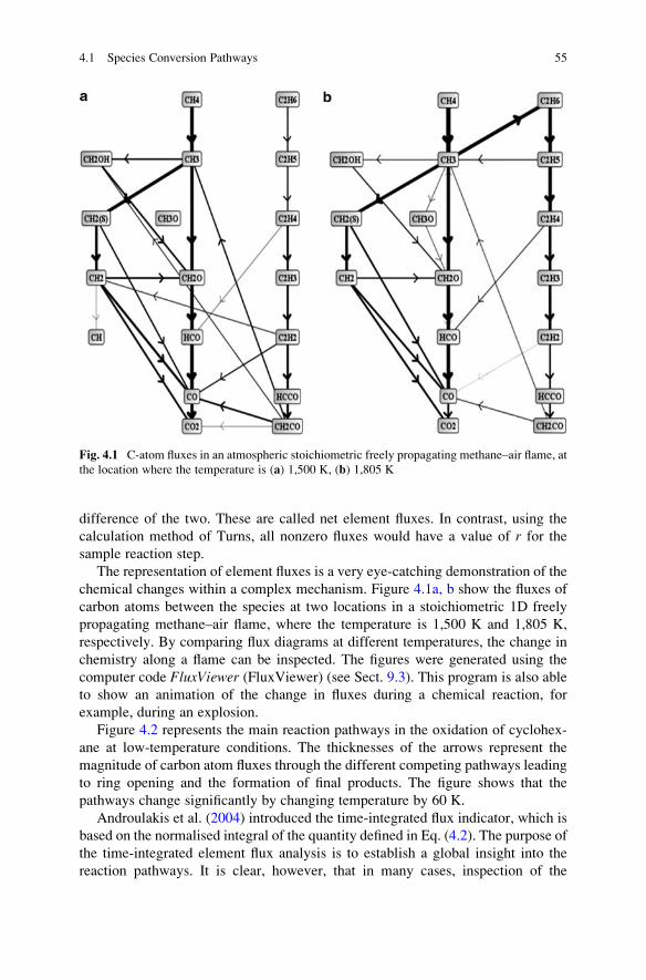
http://dx.doi.org/10.1007/978-3-662-44562-4_5#Fig4



difference of the two. These are called net element fluxes. In contrast, using the

calculation method of Turns, all nonzero fluxes would have a value of r for the

sample reaction step.

The representation of element fluxes is a very eye-catching demonstration of the

chemical changes within a complex mechanism. Figure 4.1a, b show the fluxes of

carbon atoms between the species at two locations in a stoichiometric 1D freely

propagating methane–air flame, where the temperature is 1,500 K and 1,805 K,

respectively. By comparing flux diagrams at different temperatures, the change in

chemistry along a flame can be inspected. The figures were generated using the

computer code FluxViewer (FluxViewer) (see Sect. 9.3). This program is also able

to show an animation of the change in fluxes during a chemical reaction, for

example, during an explosion.

Figure 4.2 represents the main reaction pathways in the oxidation of cyclohex-

ane at low-temperature conditions. The thicknesses of the arrows represent the

magnitude of carbon atom fluxes through the different competing pathways leading

to ring opening and the formation of final products. The figure shows that the

pathways change significantly by changing temperature by 60 K.

Androulakis et al. (2004) introduced the time-integrated flux indicator, which is

based on the normalised integral of the quantity defined in Eq. (4.2). The purpose of

the time-integrated element flux analysis is to establish a global insight into the

reaction pathways. It is clear, however, that in many cases, inspection of the

Fig. 4.1 C-atom fluxes in an atmospheric stoichiometric freely propagating methane–air flame, at

the location where the temperature is (a) 1,500 K, (b) 1,805 K

4.1 Species Conversion Pathways 55


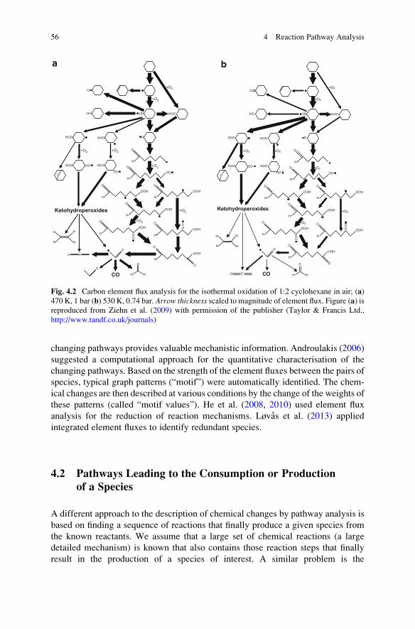
changing pathways provides valuable mechanistic information. Androulakis (2006)

suggested a computational approach for the quantitative characterisation of the

changing pathways. Based on the strength of the element fluxes between the pairs of

species, typical graph patterns (“motif”) were automatically identified. The chem-

ical changes are then described at various conditions by the change of the weights of

these patterns (called “motif values”). He et al. (2008, 2010) used element flux

analysis for the reduction of reaction mechanisms. Løvas et al. (2013) applied

integrated element fluxes to identify redundant species.

4.2 Pathways Leading to the Consumption or Productionof a Species

A different approach to the description of chemical changes by pathway analysis is

based on finding a sequence of reactions that finally produce a given species from

the known reactants. We assume that a large set of chemical reactions (a large

detailed mechanism) is known that also contains those reaction steps that finally

result in the production of a species of interest. A similar problem is the

Ketohydroperoxides

CO

OO

O

HOOHO

HOOHOO

HOO

OO

HOO

OO

O

H

O

H

OOH

O

H

OO

OOH

O

H

OOH

O

H

OOH

O

H

OO

OOH

O

H OO

OH

O

OOHO

+O2

+O2

+O2 +O2

+O2

+O2

+O2

O C

O

HH

H H

H H

O

O

O

Ketohydroperoxides

CO

OO

O

HOOHO

HOOHOO

HOO

OO

HOO

OO

O

H

O

H

OOH

O

H

OO

OOH

O

H

OOH

O

H

OOH

O

H

OO

OOH

O

H OO

O

H

O

OOHO

+O2

+O2

+O2 +O2

+O2

+O2

+O2

O C

O

HH

H H

H H

O

O

a b

Fig. 4.2 Carbon element flux analysis for the isothermal oxidation of 1:2 cyclohexane in air; (a)470 K, 1 bar (b) 530 K, 0.74 bar. Arrow thickness scaled to magnitude of element flux. Figure (a) isreproduced from Ziehn et al. (2009) with permission of the publisher (Taylor & Francis Ltd.,

http://www.tandf.co.uk/journals)


http://www.tandf.co.uk/journals

identification of pathways needed for the removal for a given species (Lehmann

2004). A representative example is the investigation of catalytic ozone destruction

cycles in the stratosphere. The grouping of reactions into pathways helps in

interpreting the interplay between the large number of reaction steps in the chem-

ical kinetic system under investigation.

The two main branches of this type of investigation differ depending on whether

(1) only the stoichiometric information (i.e. reaction equations) of the base detailed

mechanism is known or (2) kinetic data (i.e. reaction rates) are also available. For

the case when only stoichiometric information is available, a series of algorithms

were elaborated for the determination of pathways in various chemical (mainly

biochemical) reaction systems (Milner 1964; Happel and Sellers 1982; von

Hohenbalken et al. 1987; Clarke 1988; Seressiotis and Bailey 1988;

Mavrovouniotis et al. 1990; Mavrovouniotis 1992; Johnson and Corio 1993;

Schuster and Schuster 1993; Schuster and Hilgetag 1994; Schuster et al. 1999,

2002; Schilling et al. 1999, 2000). These algorithms start with the individual

reactions as separated initial pathways. Then, for each intermediate species, each

pathway producing this species is connected with each pathway consuming it. The

algorithms mainly differ in the way in which the “too complicated” pathways are

detected and eliminated. Several methods include a test that ensures that a pathway

is deleted if it includes another one as sub-pathway that contains the same set of

reactions and at least one reaction more. As these algorithms do not exploit kinetic

information (reaction rates), they cannot distinguish between important and

unimportant pathways. For large reaction systems, the total number of pathways

may become prohibitively large (“combinatorial explosion”).

Another possible approach uses not only the stoichiometric information but

assumes that the reaction rates are known. The corresponding algorithm also starts

from the basic idea of forming pathways by connecting shorter ones. Johnston and

Kinnison (1998) determined special pathways in a reaction system using reaction

rates. Their analysis was carried out manually and required an insight into the

chemical system. An algorithm for a “quick look” on the most important pathways

was presented by Lehmann (2002). This method was improved and generalised

later by the same author (Lehmann 2004).

An example for this approach is the generation of CH4 removal pathways in the

stratosphere from known reaction steps (Lehmann 2004). One possible result is the

following sequence of reactions:

CH4 þ OH þ O2 ! CH3O2 þ H2O

CH3O2 þ NO þ O2 ! CH2O þ HO2 þ NO2

CH2O þ hυ ! CO þ H2

NO þ HO2 ! NO2 þ OH

NO2 þ hυ ! NO þ O

O þ O2 ! O3

Summing up the reactions above (by taking the last two reaction steps twice) gives

the following global reaction for CH4 consumption:

4.2 Pathways Leading to the Consumption or Production of a Species 57

CH4 þ 4O2 ! 2O3 þ H2Oþ H2 þ CO

The methods described in this section looked for all reaction steps that are

needed for the explanation of the consumption (or production) of a given species.

Then, the corresponding global reaction is generated from these reaction steps. An

alternative (almost opposite) problem is when the global reaction is known and

elementary reactions are looked for that can together provide the given global

reaction. Kovacs et al. (2004) suggested a systematic method to obtain chemically

acceptable decompositions of a global reaction. The decomposition process was

based on integer programming theory considering also the restrictions of chemical

origin. The algorithm is able to decompose a global chemical reaction into elemen-

tary steps in every possible way.

The analysis of pathways and flux distributions is also becoming increasingly

common in metabolic networks and a number of online tools are available to

facilitate applications (Klamt et al. 2003; Xia and Wishart 2010). The regulation

of metabolic pathways via the optimisation of pathway fluxes is of particular

interest in the fields of pharmaceutical engineering and biotechnology (Wiechert

2002). Flux balance analysis (FBA) calculates the flow of metabolites through a

metabolic network, allowing the prediction of the growth rate of an organism or the

rate of production of a biotechnologically important metabolite (Orth et al. 2010).

Cary et al. (2005) provided a mini-review of metabolic, signalling, protein inter-

action and gene regulation pathways and referred to 170 pathway databases in

systems biology.

In many cases within systems biology, the specific values for kinetic rate

parameters are not provided or are often not known with any degree of certainty

(Lee et al. 2006). Instead, such parameters are described by constraints,

e.g. maximum and minimum allowable fluxes of the reactions, and FBA is used

in the calculation of maximum overall reaction rates or in determining extreme

pathways, i.e. the minimum number of reactions that the network requires to exist

as a functional unit (Papin et al. 2004). FBA can be used to suggest the most

efficient pathways through a steady-state network in order to achieve a particular

objective function. One example of an objective function might be the maximum

biomass growth rate. The FBA approach can also be coupled with a type of

sensitivity analysis where reactions or pairs of reactions are removed from the

network or their fluxes inhibited, and changes in the overall reactivity predicted.

This could be particularly useful in exploring the effects of drug interventions [e.g.

Becker et al. (2007)]. Pathway analysis can also be used in the optimisation of

reaction rate parameters via the comparison of a network flux model with experi-

mental observations (Mendes and Kell 1998; Hoops et al. 2006). A strategy for

large-scale model construction of kinetic models of metabolic networks based on a

logical layering of data including reaction fluxes, metabolite concentrations and

kinetic rate coefficients has recently been discussed in Stanford et al. (2013).


References

Androulakis, I.P.: New approaches for representing, analyzing and visualizing complex kinetic

transformations. Comput. Chem. Eng. 31, 41–50 (2006)

Androulakis, I.P., Grenda, J.M., Bozzelli, J.W.: Time-integrated pointers for enabling the analysis

of detailed reaction mechanisms. AIChE J. 50, 2956–2970 (2004)

Becker, S.A., Feist, A.M., Mo, M.L., Hannum, G., Palsson, B.O., Herrgard, M.J.: Quantitative

prediction of cellular metabolism with constraint-based models: the COBRA toolbox. Nat.

Protoc. 2, 727–738 (2007)

Bendtsen, A.B., Glarborg, P., Dam-Johansen, K.: Visualization methods in analysis of detailed

chemical kinetics modelling. Comput. Chem. 25, 161–170 (2001)

Boudart, M., Djega-Mariadassou, G.: Kinetics of Heterogeneous Catalytic Reactions. Princeton

University Press, Princeton (1982)

Cary, M.P., Bader, G.D., Sande, C.: Pathway information for systems biology. FEBS Lett. 579,1815–1820 (2005)

Clarke, B.L.: Stoichiometric network analysis. Cell Biophys. 12, 237–253 (1988)

Fishtik, I., Callaghan, C.A., Datta, R.: Wiring diagrams for complex reaction networks. Ind. Eng.

Chem. Res. 45, 6468–6476 (2006)

FluxViewer: Visualisation tool for element fluxes. http://garfield.chem.elte.hu/Combustion/

fluxviewer.htm

Happel, J., Sellers, P.H.: Multiple reaction mechanisms in catalysis. Ind. Eng. Chem. Fundam. 21,67–76 (1982)

He, K., Ierapetritou, M.G., Androulakis, I.P.: A graph-based approach to developing adaptive

representations of complex reaction mechanisms. Combust. Flame 155, 585–604 (2008)

He, K., Androulakis, I.P., Ierapetritou, M.G.: On-the-fly reduction of kinetic mechanisms using

element flux analysis. Chem. Eng. Sci. 65, 1173–1184 (2010)

Hoops, S., Sahle, S., Gauges, R., Lee, C., Pahle, J., Simus, N., Singhal, M., Xu, L., Mendes, P.,

Kummer, U.: COPASI—a COmplex PAthway SImulator. Bioinformatics 22, 3067–3074(2006)

Horiuti, J.: Theory of reaction rates as based on the stoichiometric number concept. Ann. N. Y.

Acad. Sci. 213, 5–30 (1973)

Johnson, B.G., Corio, P.L.: Computer construction of reaction mechnisms. J. Phys. Chem. 97,12100–12105 (1993)

Johnston, H., Kinnison, D.: Methane photooxidation in the atmosphere: contrast between two

methods of analysis. J. Geophys. Res. 103, 21967–21984 (1998)

Klamt, S., Stelling, J., Ginkel, M., Gilles, E.D.: FluxAnalyzer: exploring structure, pathways, and

flux distributions in metabolic networks on interactive flux maps. Bioinformatics 19, 261–269(2003)

Kovacs, K., Vızvari, B., Riedel, M., Toth, J.: Decomposition of the permanganate/oxalic acid

overall reaction to elementary steps based on integer programming theory. PCCP 6, 1236–1242(2004)

Lee, J.M., Gianchandani, E.P., Papin, J.A.: Flux balance analysis in the era of metabolomics. Brief.

Bioinform. 7, 140–150 (2006)

Lehmann, R.: Determination of dominant pathways in chemical reaction systems: an algorithm

and its application to stratospheric chemistry. J. Atmos. Chem. 41, 297–314 (2002)

Lehmann, R.: An algorithm for the determination of all significant pathways in chemical reaction

systems. J. Atm. Chem. 47, 45–78 (2004)

Løvas, T., Houshfar, E., Bugge, M., Skreiberg, Ø.: Automatic generation of kinetic skeletal

mechanisms for biomass combustion. Energy Fuels 27, 6979–6991 (2013)

Mavrovouniotis, M.L.: Synthesis of reaction mechanisms consisting of reversible and irreversible

steps. 2. Formalization and analysis of the synthesis algorithm. Ind. Eng. Chem. Res. 31, 1637–1653 (1992)

References 59

http://garfield.chem.elte.hu/Combustion/fluxviewer.htm


Mavrovouniotis, M.L., Stephanopoulos, G., Stephanopoulos, G.: Computer-aided synthesis of

biochemical pathways. Biotechnol. Bioeng. 36, 1119–1132 (1990)

Mendes, P., Kell, D.B.: Non-linear optimization of biochemical pathways: applications to meta-

bolic engineering and parameter estimation. Bioinformatics 14, 869–883 (1998)

Milner, P.C.: The possible mechanisms of complex reactions involving consecutive steps.

J. Electrochem. Soc. 111, 228–232 (1964)

Orth, J.D., Thiele, I., Palsson, B.O.: What is flux balance analysis? Nat. Biotechnol. 28, 245–248(2010)

Papin, J.A., Stelling, J., Price, N.D., Klamt, S., Schuster, S., Palsson, B.O.: Comparison of

network-based pathway analysis methods. Trends Biotechnol. 22, 400–405 (2004)

Revel, J., Boettner, J.C., Cathonnet, M., Bachman, J.S.: Derivation of a global chemical kinetic

mechanism for methane ignition and combustion. J. Chim. Phys. 91, 365–382 (1994)

Schilling, C.H., Schuster, S., Palsson, B.O., Heinrich, R.: Metabolic pathway analysis: basic

concepts and scientific applications in the post-genomic era. Biotechnol. Prog. 15, 296–303(1999)

Schilling, C.H., Letscher, D., Palsson, B.Ø.: Theory for the systematic definition of metabolic

pathways and their use in interpreting metabolic function from a pathway-oriented perspective.

J. Theor. Biol. 203, 229–248 (2000)

Schuster, S., Hilgetag, C.: On elementary flux modes in biochemical reaction systems at steady

state. J. Biol. Syst. 2, 165–182 (1994)

Schuster, R., Schuster, S.: Refined algorithm and computer program for calculating all nonnega-

tive fluxes admissible in steady states of biochemical reaction systems with or without some

flux rates fixed. Comp. Appl. Biosci. 9, 79–85 (1993)

Schuster, S., Danekar, T., Fell, D.A.: Detection of elementary flux modes in biochemical net-

works: a promising tool for pathway analysis and metabolic engineering. Trends Biotechnol.

17, 53–60 (1999)

Schuster, S., Hilgetag, C., Woods, J.H., Fell, D.A.: Reaction routes in biochemical reaction

systems: algebraic properties, validated calculation procedure and example from nucleotide

metabolism. J. Math. Biol. 45, 153–181 (2002)

Seressiotis, A., Bailey, J.E.: MPS: An artificially intelligent software system for the analysis and

synthesis of metabolic pathways. Biotechnol. Bioeng. 31, 587–602 (1988)

Stanford, N.J., Lubitz, T., Smallbone, K., Klipp, E., Mendes, P., Liebermeister, W.: Systematic

construction of kinetic models from genome-scale metabolic networks. PLoS One 8, e79195(2013)

Temkin, M.I.: The kinetics of some industrial heterogeneous catalytic reactions. Adv. Catal. 26,173–291 (1979)

Turns, S.R.: An Introduction to Combustion. Concepts and Applications, 2nd edn. McGraw-Hill,

Boston (2000)

von Hohenbalken, B., Clarke, B.L., Lewis, J.E.: Least distance methods for the frame of homo-

geneous equation systems. J. Comput. Appl. Math. 19, 231–241 (1987)

Wiechert, W.: Modeling and simulation: tools for metabolic engineering. J. Biotechnol. 94, 37–63(2002)

Xia, J., Wishart, D.S.: MetPA: a web-based metabolomics tool for pathway analysis and visual-

ization. Bioinformatics 26, 2342–2344 (2010)

Ziehn, T., Hughes, K.J., Griffiths, J.F., Porter, R., Tomlin, A.S.: A global sensitivity study of

cyclohexane oxidation under low temperature fuel-rich conditions using HDMR methods.

Combust. Theor. Model. 13, 589–605 (2009)


Chapter 5

Sensitivity and Uncertainty Analyses

Abstract The aim of sensitivity and uncertainty analysis methods is to determine

the influence of changes in model input parameters on the output of mathematical

models. Such methods can help to highlight key model inputs that drive uncer-

tainties in model predictions. Here we describe a range of mathematical tools for

sensitivity and uncertainty analysis which may assist in the evaluation of large

kinetic mechanisms. Approaches based on local sensitivity, local uncertainty and

global uncertainty analysis are covered, as well as examples of their application to a

variety of chemical kinetic models. Local sensitivity analysis is a routinely used

method for the investigation of models and the theory behind it is discussed.

Uncertainty analysis reveals the uncertainty of the simulation results caused by

the uncertainty of model input parameters. Such uncertainties can be estimated

using local sensitivity coefficients, but global uncertainty methods based on sam-

pling approaches usually provide more realistic results. Global sensitivity methods

can then be applied which determine how each input parameter contributes to the

overall output uncertainty based on measures such as output variance. Various

global methods for sensitivity analysis are discussed here, including the Morris

screening method, the calculation of sensitivity indices based on random sampling,

the Fourier Amplitude Sensitivity Test (FAST) method and the different surface

response methods. All of these methods can be applied generally to mathematical

models, but we also include a discussion of topics specifically related to reaction

kinetics such as uncertainties in rate coefficients and the characterisation of the

uncertainty of Arrhenius parameters.

5.1 Introduction

The term sensitivity analysis defines a collection of mathematical methods that can

be used to explore the relationships between the values of the input parameters of a

mathematical model and its solutions. Uncertainty analysis tells us how our lack of

knowledge of model inputs propagates to the predictive uncertainty of key model

outputs. This could include the equivalent of determining experimental error bars

but for model outputs. The sources of such uncertainty can include lack of



61

knowledge of the values of input parameters, errors in the measurement of key

physical inputs or even problems with the model structure itself. The latter may

stem from a lack of understanding of the chemical and physical processes

(e.g. missing chemical pathways) or our inability to represent them at a sufficiently

fundamental level such as with turbulence closure models or parameterisations of

the pressure and temperature dependence of kinetic processes. Each input param-

eter of a model is the result of measurement, theoretical calculation or estimation

and therefore will be uncertain to differing degrees. One might expect that a well-

studied parameter, i.e. one where several experimental and/or theoretical estimates

have been made which are in broad agreement, would have considerably lower

uncertainty than one which has been estimated by expert opinion or by analogy to

other parameters.

The uncertainty of a parameter can be characterised by the upper and lower limits

of the parameter or by the expected value and the variance of the parameter. Such

descriptions of individual parameter uncertainty can, for example, be obtained from

the data evaluation sources introduced in Chap. 3. The joint probability density

function (pdf) of parameters gives the most complete information about the uncer-

tainty of a parameter set. Methods of uncertainty analysis provide information about

the uncertainty of the results of a model knowing the uncertainty of its input

parameters. If such a lack of knowledge of model inputs is propagated through the

model system then a model output becomes a distribution rather than a single value.

Measures such as output variance can then be used to represent output uncertainty.

According to the formal definition of Saltelli and co-workers (2000), sensitivity

coefficients represent the contribution of the uncertainty of each individual para-

meters to the overall predictive uncertainty of the model results. To apply this

definition, the uncertainty ranges of the input parameters need to be known in order

to carry out a full sensitivity analysis. However, it is still possible to explore the

response of a model to changes in input parameters even if the range of possible

values for these parameters is not fully known. For example, we can adjust the

values of the input parameters by a fixed amount and investigate the model

response. This more general definition of sensitivity analysis is the one more

commonly adopted within the literature, and often all parameters are varied by

the same (absolute or relative) factors, negating the need for defining uncertainty

ranges. This type of analysis highlights the key processes, independently of the

information on the uncertainty of parameters.

A comprehensive monograph (Saltelli et al. 2000) and a textbook (Saltelli

et al. 2008) were recently published about the methods of sensitivity analysis as

well as practical guide to their application (Saltelli et al. 2004, 2008). In chemical

kinetics, applications of sensitivity analysis were discussed in several reviews

(Rabitz et al. 1983; Turanyi 1990; Tomlin et al. 1997; Saltelli et al. 2005, 2012;

Tomlin 2013; Tomlin and Turanyi 2013). Applications of sensitivity analysis in

systems biology were reviewed by Zi (2011), Charzynska et al. (2012) and

Puszynski et al. (2012).

The most frequently applied method is local sensitivity analysis (Turanyi 1997;

Turanyi and Rabitz 2000) where the response of the model output to a small

62 5 Sensitivity and Uncertainty Analyses

parameter change close to the nominal value of the parameter is explored. How-

ever, there are some disadvantages of using this more simplistic approach to

sensitivity analysis which will be highlighted in the following discussion of local

versus global methods.

In this book we mainly discuss deterministic kinetic models based on differential

equations. The stochastic simulation of chemical kinetic models was only men-

tioned briefly in Sect. 2.1.3. We note that it is also possible to investigate stochastic

models by sensitivity analysis and we refer the readers to the articles of Gunawan

et al. (2005), Degasperi and Gilmore (2008), Charzynska et al. (2012) and Pantazis

et al. (2013).

Before we discuss the available mathematical methods, it is worthwhile to

consider first why we might go to the trouble of performing sensitivity and

uncertainty analysis of a model. In the evaluation of any complex model, we may

be interested in knowing the confidence that can be placed in its predictions. If we

are to use the model as a design tool, then this could be quite important. We may not

wish to base important decisions on a model that has a low predictive capability. If

the predictive uncertainty of the model is high, and perhaps it gives poor agreement

with available experimental data, then we may need to develop strategies to

improve the model. For large models with very many parameters, it is sometimes

difficult to know where to start; i.e. which parameter should we remeasure first in

order to reduce its uncertainty and therefore improve our confidence in the model

predictions. Methods which allow the determination of parameter importance can

help us to focus our efforts for model improvement on those parameters that have

the biggest influence on the predicted outputs. This approach has been recently

demonstrated in the field of combustion through the coupling of global sensitivity

analysis with high-level quantum chemistry and transition-state-theory calculations

for important reactions in the case of methanol ignition (Skodje et al. 2010).

Finally, sensitivity analysis can help us to better understand the chemical processes

within our model and to identify those pathways which determine key model

outputs or product distributions. In fact, one might argue that no model validation

is complete without some kind of sensitivity analysis, since good agreement

between model and experiment does not necessarily imply accurate parameter-

isation of the model. The effects of errors in different parameters may sometimes

cancel, thus masking their individual effects. This point will be further discussed in

Chap. 8.

5.2 Local Sensitivity Analysis

5.2.1 Basic Equations

For a spatially homogeneous, dynamical system, the change of the concentrations

in time can be calculated by solving the following initial value problem:

5.2 Local Sensitivity Analysis 63


http://dx.doi.org/10.1007/978-3-662-44562-4_8

dY

dt¼ f Y; xð Þ, Y t0ð Þ ¼ Y0 ð5:1Þ

where the parameter vector x having m elements may include rate coefficients,

Arrhenius parameters, thermodynamic data, etc. Note that Eq (2.9) was copied here

to make this chapter self-contained.

Let us now look at the effect of changing parameter values on the solution over

time. Assume that the solution of the system of differential equations (5.1) is

calculated from time t¼ 0 to time t¼ tl. Here the value of parameter j is changedby Δxj and the solution of the ODE is continued until time t2 (see Fig. 5.1). We

denote Yi(t2) as the original solution and eYi t2ð Þ as the modified solution at time t2.The sensitivity coefficient can be approximately calculated by a finite-difference

approximation:

∂Yi

∂xjt1; t2ð Þ � ΔYi t2ð Þ

Δxj¼eYi t2ð Þ � Yi t2ð Þ

Δxjð5:2Þ

The effect of changes in parameter set x on the concentrations at a given time can

be characterised by the following Taylor expansion:

Yi t, xþ Δxð Þ ¼ Yi t; xð Þ þXmj¼1

∂Yi

∂xjΔxj þ 1

2

Xmk¼1

Xmj¼1

∂2Yi

∂xk∂xjΔxkΔxj þ . . . ð5:3Þ

Here the partial derivative ∂Yi/∂xj is called the first-order local sensitivity coeffi-cient, the second-order partial derivative ∂2Yi/∂xk∂xj is called the second-order

local sensitivity coefficient, etc. Commonly only the first-order linear sensitivity

coefficients ∂Yi/∂xj are calculated and interpreted, although we will see in

Sect. 5.6.5 that this may cause problems in some cases. The local sensitivity

Fig. 5.1 Solution of a

kinetic simulation (solidline) and the effect when

one of the parameters is

changed at time t1 (dashedline). The differencebetween the two solutions is

ΔYi at time t2


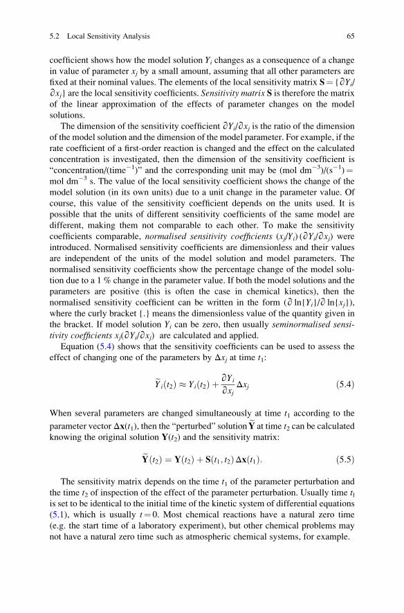
coefficient shows how the model solution Yi changes as a consequence of a changein value of parameter xj by a small amount, assuming that all other parameters are

fixed at their nominal values. The elements of the local sensitivity matrix S¼ {∂Yi/∂xj} are the local sensitivity coefficients. Sensitivity matrix S is therefore the matrix

of the linear approximation of the effects of parameter changes on the model

solutions.

The dimension of the sensitivity coefficient ∂Yi/∂xj is the ratio of the dimension

of the model solution and the dimension of the model parameter. For example, if the

rate coefficient of a first-order reaction is changed and the effect on the calculated

concentration is investigated, then the dimension of the sensitivity coefficient is

“concentration/(time�1)” and the corresponding unit may be (mol dm�3)/(s�1)¼mol dm�3 s. The value of the local sensitivity coefficient shows the change of the

model solution (in its own units) due to a unit change in the parameter value. Of

course, this value of the sensitivity coefficient depends on the units used. It is

possible that the units of different sensitivity coefficients of the same model are

different, making them not comparable to each other. To make the sensitivity

coefficients comparable, normalised sensitivity coefficients (xj/Yi) (∂Yi/∂xj) wereintroduced. Normalised sensitivity coefficients are dimensionless and their values

are independent of the units of the model solution and model parameters. The

normalised sensitivity coefficients show the percentage change of the model solu-

tion due to a 1 % change in the parameter value. If both the model solutions and the

parameters are positive (this is often the case in chemical kinetics), then the

normalised sensitivity coefficient can be written in the form (∂ ln{Yi}/∂ ln{xj}),where the curly bracket {.} means the dimensionless value of the quantity given in

the bracket. If model solution Yi can be zero, then usually seminormalised sensi-tivity coefficients xj(∂Yi/∂xj) are calculated and applied.

Equation (5.4) shows that the sensitivity coefficients can be used to assess the

effect of changing one of the parameters by Δxj at time t1:

eYi t2ð Þ � Yi t2ð Þ þ ∂Yi

∂xjΔxj ð5:4Þ

When several parameters are changed simultaneously at time t1 according to the

parameter vector Δx(t1), then the “perturbed” solution eY at time t2 can be calculatedknowing the original solution Y(t2) and the sensitivity matrix:

eY t2ð Þ ¼ Y t2ð Þ þ S t1; t2ð ÞΔx t1ð Þ: ð5:5Þ

The sensitivity matrix depends on the time t1 of the parameter perturbation and

the time t2 of inspection of the effect of the parameter perturbation. Usually time tlis set to be identical to the initial time of the kinetic system of differential equations

(5.1), which is usually t¼ 0. Most chemical reactions have a natural zero time

(e.g. the start time of a laboratory experiment), but other chemical problems may

not have a natural zero time such as atmospheric chemical systems, for example.


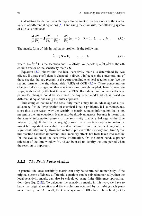
Calculating the derivative with respect to parameter xj of both sides of the kineticsystem of differential equations (5.1) and using the chain rule, the following system

of ODEs is obtained:

d

dt

∂Y∂xj

¼ J∂Y∂xj

þ ∂f∂xj

,∂Y∂xj

t0ð Þ ¼ 0 j ¼ 1, 2, . . . , Nð Þ: ð5:6Þ

The matrix form of this initial value problem is the following:

_S ¼ J Sþ F, S 0ð Þ ¼ 0; ð5:7Þ

where J¼∂f/∂Y is the Jacobian and F¼∂f/∂x. We denote si¼∂Yi/∂x as the i-thcolumn vector of the sensitivity matrix S.

Equation (5.7) shows that the local sensitivity matrix is determined by two

effects. If a rate coefficient is changed, it directly influences the concentrations of

those species that are present in the corresponding chemical reaction step (see the

second term on the right-hand side (RHS) of ODE (5.7)). These concentration

changes induce changes in other concentrations through coupled chemical reaction

steps, as dictated by the first term of the RHS. Both direct and indirect effects of

parameter changes could be identified for any other model which is based on

differential equations using a similar approach.

This complex nature of the sensitivity matrix may be an advantage or a dis-

advantage for the investigation of chemical kinetic problems. It is advantageous,

since this is the reason why the sensitivity matrix contains information that is not

present in the rate equations. It may also be disadvantageous, because it means that

the kinetic information present in the sensitivity matrix S belongs to the time

interval (t1, t2). If the matrix S(tl, t2) shows that a reaction step is important, it

might be important for a short period after time t1 and thereafter it may not be

significant until time t2. However, matrix S preserves the memory until time t2 thatthis reaction had been important. This “memory effect” has to be taken into account

for the evaluation of the sensitivity information. On the other hand, a proper

selection of the time window (t1, t2) can be used to identify the time period when

the reaction is important.

5.2.2 The Brute Force Method

In general, the local sensitivity matrix can only be determined numerically. If the

original system of kinetic differential equations can be solved numerically, then the

local sensitivity matrix can also be calculated using finite-difference approxima-

tions (see Eq. (5.2)). To calculate the sensitivity matrix in this way, we have to

know the original solution and the m solutions obtained by perturbing each para-

meter one by one. All in all, the kinetic system of ODEs has to be solved (m + 1)


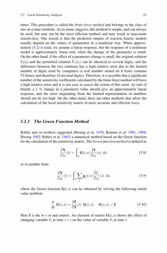
times. This procedure is called the brute force method and belongs to the class of

one-at-a-time methods. As its name suggests, this method is simple, and can always

be used, but may not be the most efficient method and may result in inaccurate

sensitivities. One reason is that the predicted outputs of reaction kinetic models

usually depend on the values of parameters in a nonlinear way. When approxi-

mation (5.2) is used, we assume a linear response, but the response of a nonlinear

model is approximately linear only when the change of the parameter is small.

On the other hand, if the effect of a parameter change is small, the original solution

Yi(t2) and the perturbed solution eYi t2ð Þ can be identical to several digits, and the

difference between the two solutions has a high relative error due to the limited

number of digits used by computers (a real number stored on 8 bytes contains

53 binary and therefore 16 decimal digits). Therefore, it is possible that a significant

number of the sensitivity coefficients calculated by the brute force method will have

a high relative error and it is not easy to assess the extent of this error. As rule of

thumb, a 1 % change in a parameter value should give an approximately linear

response, and the error originating from the limited representation of numbers

should not be too high. On the other hand, there are other methods that allow the

calculation of the local sensitivity matrix in more accurate and efficient ways.

5.2.3 The Green Function Method

Rabitz and co-workers suggested (Hwang et al. 1978; Kramer et al. 1981, 1984;

Hwang 1982; Rabitz et al. 1983) a numerical method based on the Green function

for the calculation of the sensitivity matrix. TheGreen function method is defined as

∂Y∂xk

tð Þ ¼ð t

0

G t; sð Þ ∂f∂xk

sð Þ d s ð5:8Þ

or in another form

∂Y∂xk

tð Þ ¼ð t

0

Xj

gj t; sð Þ ∂f j∂xk

sð Þ d s ð5:9Þ

where the Green function G(t, s) can be obtained by solving the following initial

value problem

d

dtG t; sð Þ ¼ ∂f

∂Ytð Þ G t; sð Þ, G s; sð Þ ¼ I ð5:10Þ

Here I is the m�m unit matrix. An element of matrix G(t, s) shows the effect of

changing variable Yj at time s< t on the value of variable Yi at time t:


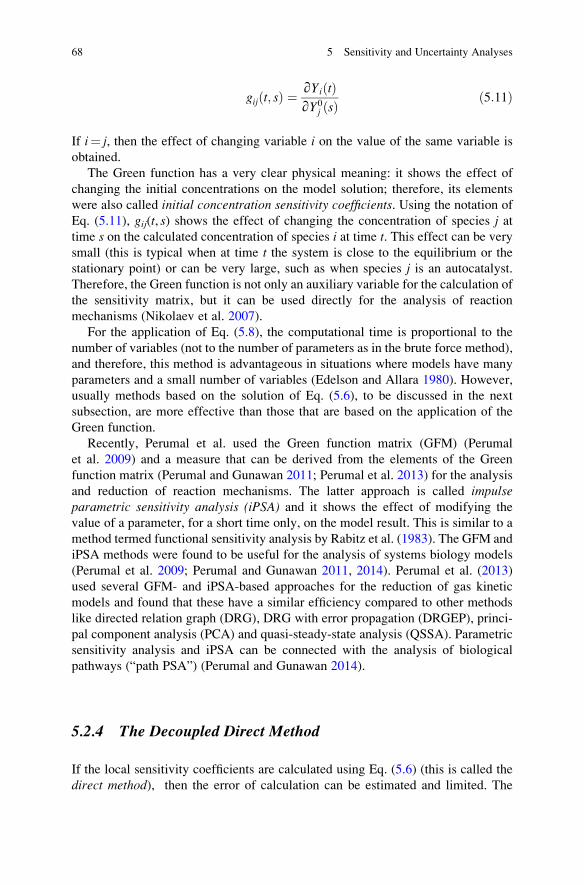
gij t; sð Þ ¼ ∂Yi tð Þ∂Y0

j sð Þ ð5:11Þ

If i¼ j, then the effect of changing variable i on the value of the same variable is

obtained.

The Green function has a very clear physical meaning: it shows the effect of

changing the initial concentrations on the model solution; therefore, its elements

were also called initial concentration sensitivity coefficients. Using the notation of

Eq. (5.11), gij(t, s) shows the effect of changing the concentration of species j attime s on the calculated concentration of species i at time t. This effect can be very

small (this is typical when at time t the system is close to the equilibrium or the

stationary point) or can be very large, such as when species j is an autocatalyst.

Therefore, the Green function is not only an auxiliary variable for the calculation of

the sensitivity matrix, but it can be used directly for the analysis of reaction

mechanisms (Nikolaev et al. 2007).

For the application of Eq. (5.8), the computational time is proportional to the

number of variables (not to the number of parameters as in the brute force method),

and therefore, this method is advantageous in situations where models have many

parameters and a small number of variables (Edelson and Allara 1980). However,

usually methods based on the solution of Eq. (5.6), to be discussed in the next

subsection, are more effective than those that are based on the application of the

Green function.

Recently, Perumal et al. used the Green function matrix (GFM) (Perumal

et al. 2009) and a measure that can be derived from the elements of the Green

function matrix (Perumal and Gunawan 2011; Perumal et al. 2013) for the analysis

and reduction of reaction mechanisms. The latter approach is called impulseparametric sensitivity analysis (iPSA) and it shows the effect of modifying the

value of a parameter, for a short time only, on the model result. This is similar to a

method termed functional sensitivity analysis by Rabitz et al. (1983). The GFM and

iPSA methods were found to be useful for the analysis of systems biology models

(Perumal et al. 2009; Perumal and Gunawan 2011, 2014). Perumal et al. (2013)

used several GFM- and iPSA-based approaches for the reduction of gas kinetic

models and found that these have a similar efficiency compared to other methods

like directed relation graph (DRG), DRG with error propagation (DRGEP), princi-

pal component analysis (PCA) and quasi-steady-state analysis (QSSA). Parametric

sensitivity analysis and iPSA can be connected with the analysis of biological

pathways (“path PSA”) (Perumal and Gunawan 2014).

5.2.4 The Decoupled Direct Method

If the local sensitivity coefficients are calculated using Eq. (5.6) (this is called the

direct method), then the error of calculation can be estimated and limited. The


difficulty of the application of Eq. (5.6) is that its usage requires the prior solution of

the kinetic system of ODEs (5.1), since the values of the elements of matrices J and

F can be calculated only if the values of the variables are known. The kinetic system

of ODEs (5.1) can be solved (Dickinson and Gelinas 1976) together with the

sensitivity ODEs (5.6) for the first parameter, then repeated for the second, third,

etc. parameters up to the m-th parameter. This means that the kinetic system of

ODEs (5.1) is unnecessarily solved (m� 1) times, since each time the sensitivity

equation is solved, the concentration�time functions are also recalculated. Another

possible approach is to solve the kinetic system of ODEs (5.1) only once, storing the

solution in a table, then to look up the actual values of variables in the table needed

for the evaluation of matrices J and F. However, this method is computationally

time consuming and can be inaccurate.

The most efficient method for the calculation of local sensitivities is the

decoupled direct method (DDM) suggested by Dunker (1981, 1984). The essence

of this method is that stiff ODE solvers select the local stepsize based on the

Jacobian (see Sect. 6.7). The Jacobian matrices of Eqs. (5.1) and (5.6) are identical.

According to the DDM algorithm, the solver converts the Jacobian of Eq. (5.1) to an

upper or lower triangular matrix, selects stepsize Δt and then calculates the new

values of variable vector Y at the new time. Using these new Y(t+Δt) values, thecode calculates the RHS of Eq. (5.6) for the first parameter and the local sensitivity

coefficients belonging to this parameter using the previously calculated triangular

matrix. The calculations of the sensitivity coefficients are then repeated for the

other parameters before taking a new time step. The most time-consuming part of

the solution of stiff ODEs is the conversion of the Jacobian to a triangular matrix,

and therefore, the DDM algorithm results in huge computational time savings.

Typically, calculating the local sensitivity coefficients for several hundred para-

meters may require only 2–3 times more computer time than a single solution of the

kinetic system of ODEs (5.1). Stiff ODE solvers can control the error of the solution

for each time step, allowing the estimation and (if needed) a decrease in the error of

the calculated sensitivities.

5.2.5 Automatic Differentiation

More recently, automatic differentiation (AD) techniques have been introduced for

the calculation of concentration sensitivities. In general these methods have been

more commonly applied in atmospheric and air quality models, possibly because

they are often linked to data assimilation methods (Zhang et al. 1998; He

et al. 2000; Djouad et al. 2003). The methods provide advantages over the finite-

difference-based brute force method since they can calculate the required deri-

vatives up to machine precision. The methods rely on the fact that any function that

is calculated on a computer is basically a sequence of simple operations such as



additions, multiplications and elementary functions such as sines and cosines. By

applying the chain rule over and over again to these simple operations, it is possible

to calculate the derivatives of a function f to machine precision in a completely

automatic way. Given the function subroutine in say Fortran, the available program

packages can produce a subroutine describing the required derivatives that can be

used to calculate various sensitivity measures. A detailed description of the avail-

able methods can be found in Bischof et al. (1996). Several packages for AD are

available in Fortran and C such as ADIFOR [automatic differentiation in Fortran

(Bischof et al. 1996; Isukapalli et al. 2000)], ADIC (Bischof et al. 1997) and

ODYSSEE (Faure 2005). Recent AD applications of relevance to combustion

modelling include a comparison of the relative sensitivities of transport properties

and reaction rates in premixed laminar flames using ADIFOR (Brown and Revzan

2005) and the analysis of the sensitivity to turbulence model parameters within the

FLUENT software environment (Bischof et al. 2004). The method has also been

extended for the solution of design optimisation problems (Hovland et al. 2005).

Another example of the use of AD is in the calculation of the Jacobian used

by the decoupled direct method. AD can provide a more automatic approach

compared to using an analytic or symbolic expression for the definition of the

Jacobian based on the RHS of the kinetic system of differential equations, but one

which is more accurate than defining the Jacobian numerically using finite-

difference methods. This approach is implemented in the freely available KPP

package for atmospheric chemical simulations (Damian et al. 2002; Sandu

et al. 2003; Daescu et al. 2003; KPP).

5.2.6 Application to Oscillating Systems

Oscillating reactions are of central importance in chemical nonlinear dynamics and

for the explanation of many biological phenomena (e.g. cell cycles, circadian

rhythm). The sensitivity functions of oscillating reactions are continuously increas-

ing if the corresponding periodic time sensitivity is not zero, i.e. if the time period

of the oscillation depends on the value of any of the parameters. A truly periodic

sensitivity function can be calculated from the “raw” sensitivity function and a

linearly increasing term (Edelson and Thomas 1981; Larter 1983; Zak et al. 2005;

Lu and Yue 2010):

Sc ¼ Sþ t

τf sTτ ð5:12Þ

Here Sc is the cleaned out (periodic) sensitivity matrix, S is the original (inflating)

sensitivity matrix, t is time, τ is the time period of the oscillation, f is the RHS of the

ODE and sτ is the vector of period sensitivities. The elements of vector sτ are the

sensitivities of the periodic time τ with respect to the parameters:


sτ ¼ ∂τ∂x1

,∂τ∂x2

, . . . ,∂τ∂xm

,

� �Tð5:13Þ

The accuracy of the decomposition in equation (5.12) depends on the accuracy of

the determination of the period sensitivity vector sτ. Several methods have been

proposed for the accurate calculation of sτ, including the application of an approx-

imate term (Edelson and Thomas 1981), a more accurate integral method (Larter

1983) and the singular value decomposition (SVD) of the original sensitivity matrix

S (Zak et al. 2005).

The transformation above is very important for the investigation of oscillatory

systems, because the original sensitivity matrix S is not very informative, whilst the

period sensitivity vector sτ shows the effect of parameters on the periodic time and

the cleaned out sensitivity matrix Sc carries information about the change of shape

of the closed trajectory in the space of variables due to the parameter changes.

Examples of the application of sensitivity analysis to oscillating systems include the

investigation of oscillatory signalling (Ihekwaba et al. 2004) and circadian clock

mechanisms (Leloup and Goldbeter 2004; Stelling et al. 2004; Ingalls 2004;

Wilkins et al. 2007).

5.3 Principal Component Analysis of the Sensitivity Matrix

Elements of the local concentration sensitivity matrix show the effect of changing a

single parameter on the calculated concentration of a species. However, we are

frequently interested in the effect of parameter changes on the concentrations of a

group of species. This effect is indicated by the overall sensitivity measure (Vajda

et al. 1985):

Bj ¼Xi

xjYi

∂Yi

∂xjtð Þ

� �2

ð5:14Þ

Quantity Bj shows the effect of changing parameter xj on the concentration of all

species present in the summation at time t (Whitehouse et al. 2004a, b). The

utilisation of such overall sensitivity measures for identifying unimportant species

or reactions as part of the model reduction process will be discussed further in

Sect. 7.2.3.

If a group of species is important for us in the time interval [t1, t2] (e.g. theconcentrations of these species can be measured in this interval), we may be

interested in which parameters or groups of parameters are highly influential on

the measured concentrations. To answer this question, the following scalar valued

function, called the objective function, will be used:

5.3 Principal Component Analysis of the Sensitivity Matrix 71


Q xð Þ ¼ðt2t1

Xi

eYi tð Þ � Yi tð ÞYi tð Þ

!2

dt ð5:15Þ

where Yi(t) is the value of variable i at time t calculated by the original parameter set

and eYi tð Þ is the corresponding value calculated with the altered parameter set. The

objective function shows the relative deviation of the two values, integrated over

time interval [t1, t2].The principal component analysis of matrix S (PCAS) (Vajda et al. 1985)

investigates the effect of the change in parameters on the value of the objective

function. The objective function Q can be approximated (Vajda et al. 1985) using

the local sensitivity matrix S:

Q αð Þ ¼ Δαð ÞTeSTeS Δαð Þ ð5:16Þ

where Δα¼Δln x, index T indicates the transpose and matrix eS is defined in the

following way:

eS ¼eS1eS2

⋮eSl

26643775 ð5:17Þ

Sensitivity matrices eSm ¼ ∂lnYi tmð Þ=∂lnxkf g belong to a series of l time points

within time interval [t1, t2], and the rows of these matrices belong to the variables

present in the summation of the objective function in Eq. (5.15). From the calcu-

lation of matrix eSTeS, the sum of the elements of matrices eSm is obtained, and

therefore the integral present in Eq. (5.15) is replaced by a summation in Eq. (5.16).

A domain of the parameters can be defined by specifying that the value of the

objective function is smaller thanQ1. This is equivalent to the domain of parameters

where the deviation of the solution of the modified parameter model from the

original model is below a given threshold. The deviation is calculated using

Eq. (5.15). Figure 5.2 shows that for a two-parameter system, the value of the

objective function Q(α) is zero at the original parameter values and increases for

any changes of the parameter values. The cross section of the goblet at level Q1

defines the domain of parameters belonging to deviations of not more than Q1. The

shape of the domain is (almost) arbitrary for the original objective function in

Eq. (5.15), but when the objective function is approximated by Eq. (5.16), then the

contour line for two parameters is an ellipsis (see Fig. 5.3). The corresponding

object for three parameters is an (rugby ball like) ellipsoid and for several para-

meters is a hyper-ellipsoid. The quadratic form defined by matrix eSTeS gives the

shape of the ellipsoid and its orientation in the space of parameters. This informa-

tion can be obtained by the eigenvector–eigenvalue decomposition of matrix eSTeS.


Let us denote λ as the vector of eigenvalues of matrix eSTeS and U the matrix of

eigenvectors. Another form of the objective function in Eq. (5.16) is the following:

Q αð Þ ¼Xi

λi ΔΨ ið Þ2 ð5:18Þ

where the transformed parameters ΔΨ¼UTΔα are called principal components.

The largest eigenvalue is related to the shortest axis of the ellipsoid, whilst the

corresponding eigenvector defines the direction of the axis. The second largest

eigenvalue is related to the second shortest axis of the ellipsoid, and the

corresponding eigenvector defines the direction of this axis, etc. If an axis of the

ellipsoid is short, this means that by changing the parameters together towards this

direction, a large change in the objective function can be obtained. Therefore, the

eigenvector belonging to the largest eigenvalue defines a parameter group, in which

the parameters changing together have the highest influence, whilst the eigenvalue

u2

Da1

Da2

u1

Fig. 5.3 The ellipsis

(or hyper-ellipsoid) defined

by the objective function

Q(α) can be characterised

by the length and the

direction of the axes (Vajda

et al. 1985)

Q(a)

a2

a1

Q(a) = constant

02a

01a

Fig. 5.2 The value of the

objective function Q(α) iszero at the original

parameter values and

increases in all directions.

The objective function is

constant at the cross

sections of the goblet. The

geometric object defined in

this way (the grey-shadedarea) can be approximated

by an ellipsis in a

two-dimensional parameter

space and a hyper-ellipsoid

in a several-dimensional

parameter space (Vajda

et al. 1985)

5.3 Principal Component Analysis of the Sensitivity Matrix 73

characterises the effectiveness of this parameter group (Vajda et al. 1985; Perger

et al. 2003). A parameter is highly influential (which means that changing this

parameter has a high influence on the selected group of outputs), if it belongs to a

high eigenvector element of a parameter group belonging to a high eigenvalue.

Therefore, principal component analysis provides a useful way to interpret complex

sensitivity information and to identify important parameter groups that influence

selected target outputs. Its use within the context of chemical model reduction will

be further discussed in Sect. 7.3. A small eigenvalue corresponds to a long axis; this

means that changing the parameters together according to the direction of the axis

has little effect on the solution of the model. This allows the identification of

parameters participating in QSSA and partial equilibrium relations (Vajda

et al. 1985).

5.4 Local Uncertainty Analysis

The local sensitivity matrix S shows the effect of a unit change of parameter values

on the model results. This can provide useful information on the relative influence

of parameters close to their nominal values and it may also be useful to estimate

how uncertainty in these parameter values can propagate to predictive uncertainty

in model outputs. The normalised sensitivity matrix eS shows the effect of a unit

relative (e.g. 1 %) change of the parameters. If we assume that the uncertainty of the

parameters is known and can be characterised by the covariance matrix Σx, then

local uncertainty analysis is based on the application of the Gaussian error propa-

gation rule:

Σy ¼ STΣxS ð5:19Þ

This means that the covariance matrix Σy of the model solution vector Y can easily

be calculated from the local sensitivity matrix S.

For a single model result Yi depending on two parameters x1 and x2, thecorresponding equation is

σ2 Yið Þ ¼ ∂Yi

∂x1

�� 2σ2 x1ð Þ þ ∂Yi

∂x2

�� 2σ2 x2ð Þ þ 2∂Yi

∂x1

∂Yi

∂x2

�� cov x1; x2ð Þ ð5:20Þ

where σ2(x1) and σ2(x2) represent the variance of x1 and x2, respectively, and σ

2(Yi)represents the variance of the output Yi. If a group of parameters are uncorrelated,

then the resulting equation is quite simple:



σ2 Yið Þ ¼Xj

∂Yi

∂xj

� �2

σ2 xj� � ð5:21Þ

Here ∂Yi

∂xjare the local sensitivity coefficients (Turanyi 1990). This approach has

been used, for example, for the uncertainty analysis of the RADM2 tropospheric

chemical mechanism (Gao et al. 1995).

5.5 Global Uncertainty Analysis

The advantage of local uncertainty analysis is that the covariance matrix Σy of the

model solution can be quickly calculated from the sensitivity coefficients. These

methods can therefore be computationally efficient. The main disadvantage of local

uncertainty analysis is that usually the embodied information belongs to the nom-inal parameter set of the model. This is the parameter set that is considered to be the

current best state of knowledge by the authors of the model (the best expert opinion)

or simply that which is originally provided with the model. Local uncertainty

analysis can provide a useful starting point for the investigation of a chemical

model and its pathways, and gives reliable results for nonlinear models if the range

of uncertainty of the parameters is small (Scire et al. 2001). However, for many

models the input parameters are not known with low uncertainty and hence the

range of possible values can be quite broad. If the response of the model is also

nonlinear, then local uncertainty and even local sensitivity analysis can prove to be

inaccurate (Ziehn and Tomlin 2008b). In some cases, local sensitivity coefficients

can be quite different for parameter values which are sufficiently far from the

nominal ones although still within a feasible range (Ziehn et al. 2009b). The

investigation of parameter importance or model reduction based on the often

uncertain nominal values therefore becomes problematic. This highlights the

necessity to develop global sensitivity methods that can provide reliable sensitivity

indices over wide ranges of model input values.

In order to apply global uncertainty and sensitivity analysis, we must assume

that the parameters of the models can be changed throughout a domain of the

parameter space rather than just a small region close to the nominal values. In the

simplest case, a range of possible values [xminj , xmax

j ] is assigned to each parameter

and this range is independent of the values of the other parameters. Parameters of

models are determined either in experiments or theoretical calculations, and some-

times have to be estimated as discussed in Chap. 3. In all cases, the parameters are

uncertain to differing extents. The most comprehensive way for the characterisation

of the uncertainty of parameters is using the joint probability density function (pdf)of all parameters.

The general task of global uncertainty analysis is to determine the joint pdf of thesimulation results knowing the joint pdf of the model parameters. The role of global

5.5 Global Uncertainty Analysis 75

sensitivity analysis is to determine the contribution of the uncertainty of each of the

parameters to the overall uncertainty of the results (Saltelli et al. 2000). Compared

to local uncertainty analysis, methods of global uncertainty analysis require more

sophisticated codes and usually much more computational time. On the other hand,

if they can be afforded, they are capable of assessing the consequences of arbitrarily

wide uncertainties in model input parameters. Because of the computational cost of

global uncertainty and sensitivity studies, several methods have been developed.

Not all methods provide all the information discussed above and each may play a

different role in a complete global analysis of a model.

5.5.1 Morris Screening Method

We start first with so-called screening methods, which may not provide a complete

set of global sensitivity coefficients but can help to identify key parameters or to

remove unimportant ones from further analysis. The best known example was

developed by Morris (1991) and Saltelli et al. (2000), and is applicable for the

identification of the most influential parameters within a model. It is classified as a

global sensitivity method since the entire parameter space over which the inputs

may vary is covered. It can also rank the degree of nonlinearity of response to

changes in each parameter by ranking the standard deviation of the parameter effect

across all parameter sets. It does not however provide the functional dependency of

the output on individual parameters or parameter pairs, and is mainly used as a way

of screening out unimportant parameters prior to the use of more informative (and

potentially more computationally intensive) methods. In the following, the version

of the Morris method modified by Campolongo et al. (2005) is discussed. The

Morris method can be encoded effectively using a linear algebra-based algorithm

(Campolongo et al. 2005). This linear algebraic formalism disguises the point of the

method, and therefore, a simpler scalar formalism will be presented here, which is

also visualised in Fig. 5.4.

Using the Morris method, a series of parameter sets are generated so that the next

parameter set differs from the previous one in the value of a single parameter only,

which is randomly chosen. The value of each parameter xj is modified within the

range [xminj , xmax

j ] by a fixed amount Δ that is determined in the following way. A

vector 0, 1q�1

, 2q�1

, 3q�1

, . . . , 1n o

is generated using a small even number q selected

by the user. Then, zero and one are assigned to the smallest and largest possible

values xminj and xmax

j of the parameter, respectively. All other values of the para-

meters are scaled linearly according to the elements of the vector above. The first

parameter set is randomly selected from the values determined by the vector. The

next parameter set is identical to the previous one, except for the value of a single

parameter as illustrated in Fig. 5.4. The value of this parameter has been moved

randomly to another possible value. The next parameter set is obtained by changing


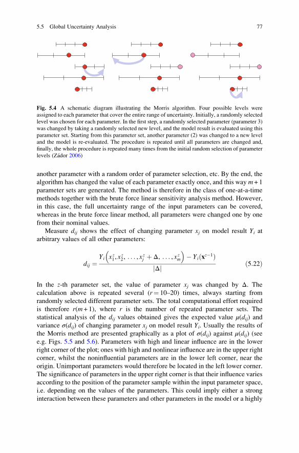
another parameter with a random order of parameter selection, etc. By the end, the

algorithm has changed the value of each parameter exactly once, and this way m + 1

parameter sets are generated. The method is therefore in the class of one-at-a-time

methods together with the brute force linear sensitivity analysis method. However,

in this case, the full uncertainty range of the input parameters can be covered,

whereas in the brute force linear method, all parameters were changed one by one

from their nominal values.

Measure dij shows the effect of changing parameter xj on model result Yi atarbitrary values of all other parameters:

dij ¼Yi x z1, x

z2, . . . , x

zj þ Δ, . . . , xzm

� Yi x

z�1ð ÞΔj j ð5:22Þ

In the z-th parameter set, the value of parameter xj was changed by Δ. The

calculation above is repeated several (r¼ 10–20) times, always starting from

randomly selected different parameter sets. The total computational effort required

is therefore r(m + 1), where r is the number of repeated parameter sets. The

statistical analysis of the dij values obtained gives the expected value μ(dij) andvariance σ(dij) of changing parameter xj on model result Yi. Usually the results of

the Morris method are presented graphically as a plot of σ(dij) against μ(dij) (seee.g. Figs. 5.5 and 5.6). Parameters with high and linear influence are in the lower

right corner of the plot; ones with high and nonlinear influence are in the upper right

corner, whilst the noninfluential parameters are in the lower left corner, near the

origin. Unimportant parameters would therefore be located in the left lower corner.

The significance of parameters in the upper right corner is that their influence varies

according to the position of the parameter sample within the input parameter space,

i.e. depending on the values of the parameters. This could imply either a strong

interaction between these parameters and other parameters in the model or a highly

Fig. 5.4 A schematic diagram illustrating the Morris algorithm. Four possible levels were

assigned to each parameter that cover the entire range of uncertainty. Initially, a randomly selected

level was chosen for each parameter. In the first step, a randomly selected parameter (parameter 3)

was changed by taking a randomly selected new level, and the model result is evaluated using this

parameter set. Starting from this parameter set, another parameter (2) was changed to a new level

and the model is re-evaluated. The procedure is repeated until all parameters are changed and,

finally, the whole procedure is repeated many times from the initial random selection of parameter

levels (Zador 2006)


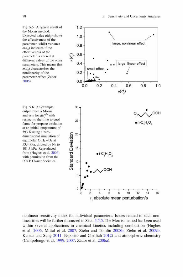
nonlinear sensitivity index for individual parameters. Issues related to such non-

linearities will be further discussed in Sect. 5.5.5. The Morris method has been used

within several applications in chemical kinetics including combustion (Hughes

et al. 2006; Mittal et al. 2007; Ziehn and Tomlin 2008b; Ziehn et al. 2009b;

Kumar and Sung 2011; Esposito and Chelliah 2012) and atmospheric chemistry

(Campolongo et al. 1999, 2007; Zador et al. 2006a).

Fig. 5.5 A typical result of

the Morris method.

Expected value μ(dij) showsthe effectiveness of the

parameter, whilst variance

σ(dij) indicates if theeffectiveness of the

parameter is altered at

different values of the other

parameters. This means that

σ(dij) characterises thenonlinearity of the

parameter effect (Zador

2006)

Fig. 5.6 An example

output from a Morris

analysis for ΔHf⦵ with

respect to the time to cool

flame for propane oxidation

at an initial temperature of

593 K using a zero-

dimensional simulation of

equimolar C3H8 +O2 at

53.4 kPa, diluted by N2 to

101.3 kPa. Reproduced

from (Hughes et al. 2006)

with permission from the

PCCP Owner Societies


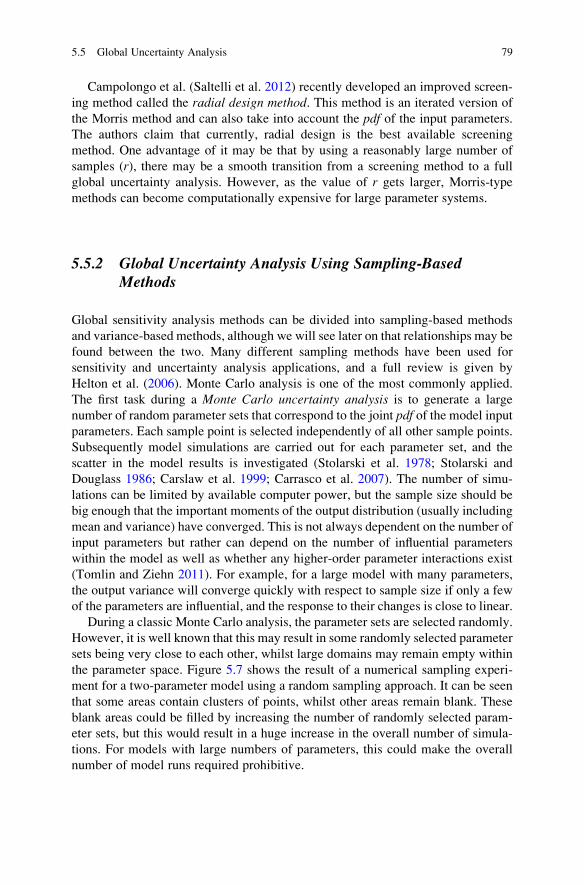
Campolongo et al. (Saltelli et al. 2012) recently developed an improved screen-

ing method called the radial design method. This method is an iterated version of

the Morris method and can also take into account the pdf of the input parameters.

The authors claim that currently, radial design is the best available screening

method. One advantage of it may be that by using a reasonably large number of

samples (r), there may be a smooth transition from a screening method to a full

global uncertainty analysis. However, as the value of r gets larger, Morris-type

methods can become computationally expensive for large parameter systems.

5.5.2 Global Uncertainty Analysis Using Sampling-BasedMethods

Global sensitivity analysis methods can be divided into sampling-based methods

and variance-based methods, although we will see later on that relationships may be

found between the two. Many different sampling methods have been used for

sensitivity and uncertainty analysis applications, and a full review is given by

Helton et al. (2006). Monte Carlo analysis is one of the most commonly applied.

The first task during a Monte Carlo uncertainty analysis is to generate a large

number of random parameter sets that correspond to the joint pdf of the model input

parameters. Each sample point is selected independently of all other sample points.

Subsequently model simulations are carried out for each parameter set, and the

scatter in the model results is investigated (Stolarski et al. 1978; Stolarski and

Douglass 1986; Carslaw et al. 1999; Carrasco et al. 2007). The number of simu-

lations can be limited by available computer power, but the sample size should be

big enough that the important moments of the output distribution (usually including

mean and variance) have converged. This is not always dependent on the number of

input parameters but rather can depend on the number of influential parameters

within the model as well as whether any higher-order parameter interactions exist

(Tomlin and Ziehn 2011). For example, for a large model with many parameters,

the output variance will converge quickly with respect to sample size if only a few

of the parameters are influential, and the response to their changes is close to linear.

During a classic Monte Carlo analysis, the parameter sets are selected randomly.

However, it is well known that this may result in some randomly selected parameter

sets being very close to each other, whilst large domains may remain empty within

the parameter space. Figure 5.7 shows the result of a numerical sampling experi-

ment for a two-parameter model using a random sampling approach. It can be seen

that some areas contain clusters of points, whilst other areas remain blank. These

blank areas could be filled by increasing the number of randomly selected param-

eter sets, but this would result in a huge increase in the overall number of simula-

tions. For models with large numbers of parameters, this could make the overall

number of model runs required prohibitive.


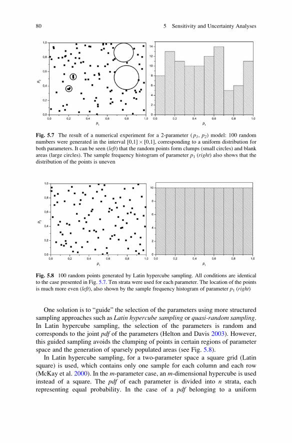
One solution is to “guide” the selection of the parameters using more structured

sampling approaches such as Latin hypercube sampling or quasi-random sampling.In Latin hypercube sampling, the selection of the parameters is random and

corresponds to the joint pdf of the parameters (Helton and Davis 2003). However,

this guided sampling avoids the clumping of points in certain regions of parameter

space and the generation of sparsely populated areas (see Fig. 5.8).

In Latin hypercube sampling, for a two-parameter space a square grid (Latin

square) is used, which contains only one sample for each column and each row

(McKay et al. 2000). In the m-parameter case, an m-dimensional hypercube is used

instead of a square. The pdf of each parameter is divided into n strata, each

representing equal probability. In the case of a pdf belonging to a uniform

Fig. 5.7 The result of a numerical experiment for a 2-parameter ( p1, p2) model: 100 random

numbers were generated in the interval [0,1]� [0,1], corresponding to a uniform distribution for

both parameters. It can be seen (left) that the random points form clumps (small circles) and blank

areas (large circles). The sample frequency histogram of parameter p1 (right) also shows that the

distribution of the points is uneven

Fig. 5.8 100 random points generated by Latin hypercube sampling. All conditions are identical

to the case presented in Fig. 5.7. Ten strata were used for each parameter. The location of the points

is much more even (left), also shown by the sample frequency histogram of parameter p1 (right)


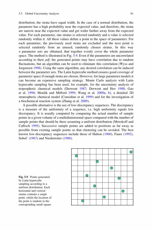
distribution, the strata have equal width. In the case of a normal distribution, the

parameter has a high probability near the expected value, and therefore, the strata

are narrow near the expected value and get wider further away from the expected

value. For each parameter, one stratus is selected randomly and a value is selected

randomly within it. All these values define a point in the space of parameters. For

each parameter, the previously used strata are excluded and the next point is

selected randomly from an unused, randomly chosen stratus. In this way

n parameter sets are obtained, that together evenly cover the whole parameter

space. The method is illustrated in Fig. 5.9. Even if the parameters are uncorrelated

according to their pdf, the generated points may have correlation due to random

fluctuations, but an algorithm can be used to eliminate this correlation (Wyss and

Jorgensen 1998). Using the same algorithm, any desired correlation can be induced

between the parameter sets. The Latin hypercube method ensures good coverage of

parameter space if enough strata are chosen. However, for large parameter models it

can become an expensive sampling strategy. Monte Carlo analysis with Latin

hypercube sampling has been used, for example, for the uncertainty analysis of

tropospheric chemical models (Derwent 1987; Derwent and Hov 1988; Gao

et al. 1996; Moulik and Milford 1999; Wang et al. 2000a, b), a detailed 2D

stratospheric chemical model (Considine et al. 1999) and for the investigation of

a biochemical reaction system (Zhang et al. 2009).

A possible alternative is the use of low-discrepancy sequences. The discrepancy

is a measure of the uniformity of a sequence, i.e. high uniformity equals low

discrepancy. It is usually computed by comparing the actual number of sample

points in a given volume of a multidimensional space compared with the number of

sample points that should be there assuming a uniform distribution (Morokoff and

Caflisch 1995). Successive sample points are added to positions as far away as

possible from existing sample points so that clustering can be avoided. The best

known low-discrepancy sequences include those of Halton (1960), Faure (1992),

Sobol’ (1967) and Niederreiter (1988).

Fig. 5.9 Points generated

by Latin hypercube

sampling according to a

uniform distribution. Each

horizontal and vertical

stratus contains a single

point, whilst the location of

the point is random in the

corresponding small square


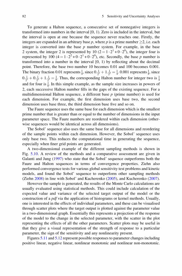
To generate a Halton sequence, a consecutive set of nonnegative integers is

transformed into numbers in the interval [0, 1). Zero is included in the interval, but

the interval is open at one because the sequence never reaches one. Firstly, the

integers are expanded in an arbitrary base p, where p is a prime number�2, i.e. each

integer is converted into the base p number system. For example, in the base

2 system, the integer 2 is represented by 10 (2¼ 1 · 21 + 0 · 20), the integer four is

represented by 100 (4¼ 1 · 22 + 0 · 21 + 0 · 20), etc. Secondly, the base p number is

transformed into a number in the interval [0, 1) by reflecting about the decimal

point. Therefore, the base two number 10 becomes 0.01 and 100 becomes 0.001.

The binary fraction 0.01 represents 14, since 0: 1

21þ 1: 1

22¼ 1

4: 0.001 represents 1

8, since

0: 121þ 0: 1

22þ 1: 1

23¼ 1

8: Thus, the corresponding Halton number for integer two is 1

4

and for four is 18. In this simple example, as the sample size increases in powers of

2, each successive Halton number fills in the gaps of the existing sequence. For a

multidimensional Halton sequence, a different base p (prime number) is used for

each dimension. For example, the first dimension uses base two, the second

dimension uses base three, the third dimension base five and so on.

The Faure sequence uses the same base for each dimension which is the smallest

prime number that is greater than or equal to the number of dimensions in the input

parameter space. The Faure numbers are reordered within each dimension (other-

wise sequences would be identical across all dimensions).

The Sobol’ sequence also uses the same base for all dimensions and reordering

of the sample points within each dimension. However, the Sobol’ sequence uses

only base two. This reduces the computational time in generating the sequence,

especially when finer grid points are generated.

A two-dimensional example of the different sampling methods is shown in

Fig. 5.10. A review of the methods and a comparative assessment are given in

Galanti and Jung (1997) who state that the Sobol’ sequence outperforms both the

Faure and Halton sequences in terms of convergence properties. Ziehn also

performed convergence tests for various global sensitivity test problems and kinetic

models, and found the Sobol’ sequence to outperform other sampling methods

(Ziehn 2008) in line with Sobol’ and Kucherenko (2005), and Kucherenko (2007).

However the sample is generated, the results of the Monte Carlo calculations are

usually evaluated using statistical methods. This could include calculation of the

expected value and variance of the selected target output of the model or the

construction of a pdf via the application of histograms or kernel methods. Usually,

one is interested in the effects of individual parameters, and these can be visualised

through scatter plots where the target output is plotted against the parameter value

in a two-dimensional graph. Essentially this represents a projection of the response

of the model to the change in the selected parameter, with the scatter in the plot

representing the effects of all the other parameters. Scatter plots may be useful in

that they give a visual representation of the strength of response to a particular

parameter, the sign of the sensitivity and any nonlinearity present.

Figures 5.11 and 5.12 represent possible responses to parameter changes including

positive linear, negative linear, nonlinear monotonic and nonlinear non-monotonic.


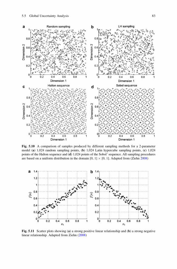
Fig. 5.11 Scatter plots showing (a) a strong positive linear relationship and (b) a strong negative

linear relationship. Adapted from Ziehn (2008)

Fig. 5.10 A comparison of samples produced by different sampling methods for a 2-parameter

model (a) 1,024 random sampling points, (b) 1,024 Latin hypercube sampling points, (c) 1,024

points of the Halton sequence and (d) 1,024 points of the Sobol’ sequence. All sampling procedures

are based on a uniform distribution in the domain [0, 1] � [0, 1]. Adapted from (Ziehn 2008)


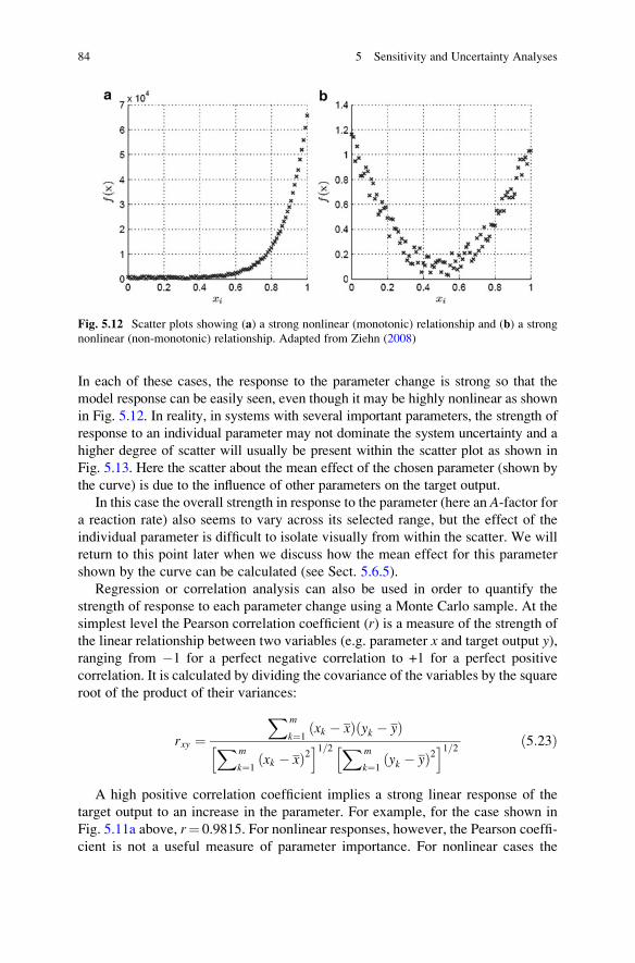
In each of these cases, the response to the parameter change is strong so that the

model response can be easily seen, even though it may be highly nonlinear as shown

in Fig. 5.12. In reality, in systems with several important parameters, the strength of

response to an individual parameter may not dominate the system uncertainty and a

higher degree of scatter will usually be present within the scatter plot as shown in

Fig. 5.13. Here the scatter about the mean effect of the chosen parameter (shown by

the curve) is due to the influence of other parameters on the target output.

In this case the overall strength in response to the parameter (here an A-factor fora reaction rate) also seems to vary across its selected range, but the effect of the

individual parameter is difficult to isolate visually from within the scatter. We will

return to this point later when we discuss how the mean effect for this parameter

shown by the curve can be calculated (see Sect. 5.6.5).

Regression or correlation analysis can also be used in order to quantify the

strength of response to each parameter change using a Monte Carlo sample. At the

simplest level the Pearson correlation coefficient (r) is a measure of the strength of

the linear relationship between two variables (e.g. parameter x and target output y),ranging from �1 for a perfect negative correlation to +1 for a perfect positive

correlation. It is calculated by dividing the covariance of the variables by the square

root of the product of their variances:

rxy ¼Xm

k¼1xk � xð Þ yk � yð ÞXm

k¼1xk � xð Þ2

h i1=2 Xm

k¼1yk � yð Þ2

h i1=2 ð5:23Þ

A high positive correlation coefficient implies a strong linear response of the

target output to an increase in the parameter. For example, for the case shown in

Fig. 5.11a above, r¼ 0.9815. For nonlinear responses, however, the Pearson coeffi-

cient is not a useful measure of parameter importance. For nonlinear cases the

Fig. 5.12 Scatter plots showing (a) a strong nonlinear (monotonic) relationship and (b) a strong

nonlinear (non-monotonic) relationship. Adapted from Ziehn (2008)


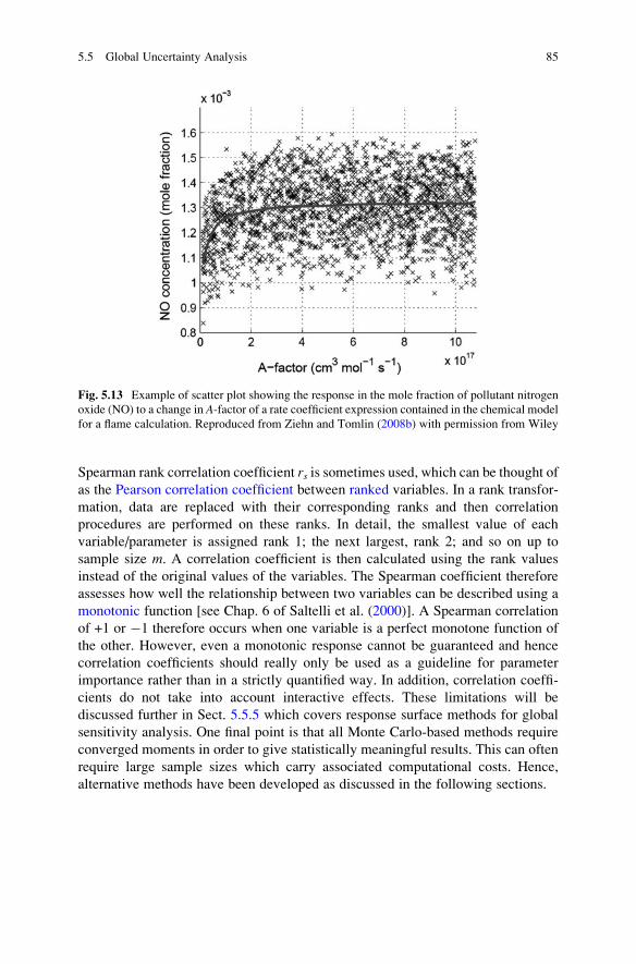
Spearman rank correlation coefficient rs is sometimes used, which can be thought of

as the Pearson correlation coefficient between ranked variables. In a rank transfor-

mation, data are replaced with their corresponding ranks and then correlation

procedures are performed on these ranks. In detail, the smallest value of each

variable/parameter is assigned rank 1; the next largest, rank 2; and so on up to

sample size m. A correlation coefficient is then calculated using the rank values

instead of the original values of the variables. The Spearman coefficient therefore

assesses how well the relationship between two variables can be described using a

monotonic function [see Chap. 6 of Saltelli et al. (2000)]. A Spearman correlation

of +1 or �1 therefore occurs when one variable is a perfect monotone function of

the other. However, even a monotonic response cannot be guaranteed and hence

correlation coefficients should really only be used as a guideline for parameter

importance rather than in a strictly quantified way. In addition, correlation coeffi-

cients do not take into account interactive effects. These limitations will be

discussed further in Sect. 5.5.5 which covers response surface methods for global

sensitivity analysis. One final point is that all Monte Carlo-based methods require

converged moments in order to give statistically meaningful results. This can often

require large sample sizes which carry associated computational costs. Hence,

alternative methods have been developed as discussed in the following sections.

Fig. 5.13 Example of scatter plot showing the response in the mole fraction of pollutant nitrogen

oxide (NO) to a change in A-factor of a rate coefficient expression contained in the chemical model

for a flame calculation. Reproduced from Ziehn and Tomlin (2008b) with permission from Wiley


http://en.wikipedia.org/wiki/Pearson_correlation_coefficient#Pearson%20correlation%20coefficient

http://en.wikipedia.org/wiki/Ranking#Ranking

http://en.wikipedia.org/wiki/Monotonic#Monotonic

5.5.3 Sensitivity Indices

The general calculation of global sensitivity indices can be based on a partial

variance method introduced by Sobol’ (1990) and Saltelli (2002). If the model

result Yi¼ fi(x1, x2, . . ., xm) is influenced by independent random parameters, then

the joint pdf of the parameters P(x1, x2, . . ., xN)¼Ymj¼1

pj xj� �

. The mean or expected

value E(Yi) of the calculated result Yi is then given by

E Yið Þ ¼ðð

. . .

ðf i x1; x2; . . . ; xmð Þ

Ymj¼1

pj xj� �

dxj ð5:24Þ

whilst the variance V(Yi) of the calculated result Yi is specified as

V Yið Þ ¼ðð

. . .

ðf i x1; x2; . . . ; xmð Þ � E Yið Þð Þ2

Ymj¼1

pj xj� �

dxj

¼ðð

. . .

ðf 2ix1; x2; . . . ; xmð Þ

Ymj¼1

pj xj� �

dxj � E2 Yið Þð5:25Þ

If the integral in Eq. (5.25) is calculated with a fixed value of a single parameter

xj, then the variance caused by all other parameters except for xj denoted by V(Yi|xj)is obtained. If this V(Yi|xj) value is calculated for many values of xj, selectedaccording to its pdf, then the expected value E(V(Yi|xj)) can be calculated. This

requires the integration of V(Yi|xj) over the pdf of xj (see Saltelli (2002) for details).The value V(Yi)–E(V(Yi|xj)) is equal to the reduced variance of Yi caused by fixing

the value of xj and is equal to V(E(Yi|xj)). Dividing this conditional variance by the

unconditional variance, the first-order sensitivity index for parameter xj can be

calculated:

Sj ið Þ ¼V E Yi xj

�� V Yið Þ ð5:26Þ

This measure shows the fraction of the total variance of Yi which is reduced when

the value of xj is held at a fixed value and is therefore a measure of the influence of

uncertainty in xj. The first-order sensitivity index is between 0 and 1, although

sometimes this is multiplied by 100 yielding Sj(i)%. The calculation of the integrals

in Eq. (5.25) is nontrivial and the use of a Monte Carlo sampling method is

described in Saltelli (2002) requiring N (2m + 1) model runs where N is the sample

size chosen for the Monte Carlo estimates.

The procedure above can be repeated so that the values of two parameters (e.g. xjand xk) are fixed and therefore second-order sensitivity indices are obtained:


Skj ið Þ ¼V E Yi xk; xj

�� V E Yi xkjð Þð Þ � V E Yi xj��

V Yið Þ ð5:27Þ

This second-order sensitivity index shows the fraction of the total variance of Yiwhich is reduced when two parameters xj and xk are fixed. In other words, the

second-order sensitivity index characterises the interaction of the corresponding

parameters. The sensitivity indices can be calculated up to an arbitrary n-th order bykeeping n parameters fixed, but the computational time requirement increases

exponentially with the order.

The total effect StotjðiÞ of parameter j can be defined as the sum of all sensitivity

indices in which parameter j is present. Assume that we have three parameters a,b and c. The total sensitivity index of parameter a is defined as

S tota ið Þ ¼ Sa ið Þ þ Sab ið Þ þ Sac ið Þ þ Sabc ið Þ ð5:28Þ

The total sensitivity index characterises the additivity of the parameters (Homma

and Saltelli 1996; Saltelli et al. 2010). If the parameters are totally additive, which

means that there are no interactions at all between the parameters, thenXmj¼1

Sj ið Þ ¼ 1

and Sj(i)¼ StotjðiÞ. This means that the variance of Yi can be fully explained by the first-

order sensitivity indices. If the parameters of the model are not additive, thenXmj¼1

Sj ið Þ < 1, and the value StotjðiÞ � Sj(i) is a measure of the interaction of the

parameters. This picture can be refined further by investigating the second- and

higher-order indices, which show the interactions of the parameters. There are also

several methods (Saltelli et al. 2010) for the direct calculation of the total sensitivity

index StotaðiÞ. Knowing the total sensitivity index, Eq. (5.28) can be used to calculate

the level of interactions of the parameters. If the first-order index is (almost) equal

to StotaðiÞ, then there is no need to calculate the higher-order indices.

This method for the calculation of sensitivity indices was developed by Sobol’

(1990), and using the original formulation, the overall characterisation of the model

would require N� 2m model runs where N is the chosen sample size and m the

number of parameters. The sample size N may be of the order of 1,000 and hence it

is easy to see that for large parameter systems this method may become very

computationally expensive. Saltelli (2002) suggested several improvements to the

algorithm, including tricks to reduce the required sample size. For example, the

evaluation of integral (5.25) in the present form is based on two cycles (one for

parameter xj and one for the other parameters), but the integral can be calculated

with a single cycle if the same parameter set is reused. The method requires N (2m+ 2) evaluations of the model for the calculation of the first-order and total indices,

where N is recommended to be between 500 and 1000. The first-order and the total

sensitivity indices have been used for the analysis of a biochemical reaction system

(Zhang et al. 2009).


Ludtke et al. (2007) developed a new version of the method above that they call

information-theoretic sensitivity analysis. Here the model is considered as a

“communication channel”, which is a transmitter of information between inputs

and outputs. Instead of analysing the variance of the output distribution, they

measured output uncertainty in terms of Shannon’s entropy. The first-order sensi-

tivity index, the higher-order sensitivity indices and the total sensitivity index all

have information-theoretic counterparts.

5.5.4 Fourier Amplitude Sensitivity Test

The Fourier Amplitude Sensitivity Test (FAST) was developed by Cukier et al. in

the 1970s and it can be considered as a special case of the more general sensitivity

index methods (Cukier et al. 1973, 1975, 1977, 1978; Schaibly and Shuler 1973).

The method was developed further by Saltelli (Saltelli and Bolado 1998). The

method is based on selecting N design points over a pre-described space-filling

curve in the m-dimensional input space, built so that each dimension (parameter) is

investigated using a different frequency [ω1,ω2,. . .,ωk] (Saltelli and Bolado 1998).

In the FAST method the m-dimensional integral in Eq. (5.24) can be transformed

to a one-dimensional integral using the following function:

xj sð Þ ¼ Gj sinωjs� � ð5:29Þ

x sð Þ ¼ G sin ωsð Þ ð5:30Þ

Here the transformation function Gj depends on the probability density function of

the corresponding parameter, the frequency ωj belonging to parameter j and the

scalar search variable s. Using function (5.30), the values of all parameters become

a periodic function of the search variable. If the frequencies ωj are relative prime

numbers, then the curve x(s) determined by Eq. (5.30) approaches all points of the

parameter space in the rectangle of uncertainty of the parameters, whilst s is

changing within the interval (�π, +π). Figure 5.14 shows how the values of the

two parameters can be changed using the appropriate sine functions, and Fig. 5.15

demonstrates that the x(s) curve searches the whole 2D parameter space of uncer-

tainty. The sine function is changing slowly near values y¼�1 and y¼ +1.

Therefore, if G is a linear function, then the sampling points defined by curve

x(s) will be denser near the edges of the parameter space.

During the FAST analysis, N parameter sets are defined by selecting N points

equidistantly in the interval�π< s< π, then the corresponding Yi model results are

calculated (once for each parameter set) and a Fourier analysis of the results is

carried out. In this way the variance fraction of the total variance of Yi can be

obtained:

V Yið Þ ¼ 2Xþ1

l¼1

A2il þ B2

il

� � ð5:31Þ


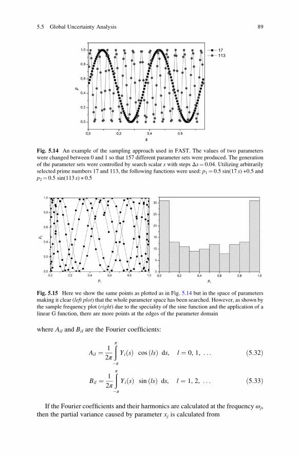
where Ail and Bil are the Fourier coefficients:

Ail ¼ 1

2π

ðπ�π

Yi sð Þ cos lsð Þ ds, l ¼ 0, 1, . . . ð5:32Þ

Bil ¼ 1

2π

ðπ�π

Yi sð Þ sin lsð Þ ds, l ¼ 1, 2, . . . ð5:33Þ

If the Fourier coefficients and their harmonics are calculated at the frequency ωj,

then the partial variance caused by parameter xj is calculated from

Fig. 5.15 Here we show the same points as plotted as in Fig. 5.14 but in the space of parameters

making it clear (left plot) that the whole parameter space has been searched. However, as shown by

the sample frequency plot (right) due to the speciality of the sine function and the application of alinear G function, there are more points at the edges of the parameter domain

Fig. 5.14 An example of the sampling approach used in FAST. The values of two parameters

were changed between 0 and 1 so that 157 different parameter sets were produced. The generation

of the parameter sets were controlled by search scalar s with steps Δs¼ 0.04. Utilizing arbitrarily

selected prime numbers 17 and 113, the following functions were used: p1¼ 0.5 sin(17 s) +0.5 andp2¼ 0.5 sin(113 s) + 0.5


Vj Yið Þ ¼ 2Xþ1

r¼1

A2i, rωj

þ B2i, rωj

ð5:34Þ

In this equation index r refers to the r-th harmonics of the base frequency ωj. The

partial variance Sij is the fraction of the total variance of the model result Yi causedby parameter xj:

Sij ¼ Vj Yið ÞV Yið Þ ð5:35Þ

The FAST method is computationally more efficient than the Sobol’ method and

may be more economical than Monte Carlo-based methods for systems with a small

number of parameters, but it is still quite time consuming. For the analysis of a

model with m parameters, N¼ 1.2m2.5 model evaluations have to be carried out

(Cukier et al. 1977). This means 21200 simulations for a 50-parameter system. If

only a small number of important parameters exist (i.e. ones which influence the

target model output), then it is possible that random or quasi-random sampling

methods may converge using a smaller sample size than that required by FAST. In

addition, the classic FAST method is used to determine first-order sensitivity

indices. Where the first-order sensitivities over all parameters sum to much less

than 1, this approach may be insufficient. For this reason an extended version of

FAST was introduced by Saltelli et al. (1999) which can be used to calculate the

total effect indices TS(i) as well as the first-order ones. TS(i) is defined as the sum of

all sensitivity indices involving the input parameter in question and is therefore a

more reliable measure of parameter importance than the first-order index if a

parameter has significant higher-order effects. However, using extended FAST, a

new set of samples is required to evaluate each of the total effect indices TS(i)(Saltelli et al. 1999) adding to the computational cost of the approach. Even so the

FAST method has been shown to be very applicable for the analysis of reaction

mechanisms (Campolongo et al. 1999). A full discussion of the FAST method, its

extensions and its applications in chemical modelling are available in Saltelli

et al. (2005) and Saltelli et al. (2012).

5.5.5 Response Surface Methods

The basic idea behind response surface methods (RSMs) is to develop a response

surface approximation which describes the relationship between the parameters in

the original model and selected target outputs. Using a sample of simulations of the

full model, a model approximation or metamodel is constructed, which can then be

used as a surrogate for the full model in order to perform uncertainty and sensitivity

analysis. The methods have some similarities with Monte Carlo approaches in that

first input parameter ranges must be selected, and then a suitable sampling approach


should be taken so that full model runs are obtained across a design which is

suitable for the development of an accurate metamodel. The results from model

evaluations using the chosen sample design are then used to construct a response

surface approximation to the real model, and sensitivity measures for the input

parameters are derived from the constructed response surface. The accuracy of the

metamodel will determine the accuracy of the calculated sensitivity indices.

The high-dimensionality of model input parameter space does not always imply

a complex functional relationship between the more influential model inputs and

target outputs. Interaction effects among more than two parameters are suggested to

be fairly rare in models of chemical systems (Rabitz and Alis 2000; Li et al. 2001),

and hence, the sample size required to develop a suitable metamodel may be much

lower than that required for the full investigation of sensitivity indices using the

Sobol’ method or the FAST method described above. For example, in a global

sensitivity study of sulphur chemistry within a doped methane flame, Ziehn and

Tomlin (2008b) found that only 5 of the 176 parameters tested in the high dimen-

sional model representation (HDMR) analysis were required to build a metamodel

giving 99.05 % of the tested samples within the 5 % relative error range compared

to the full model. To achieve a relative error of 99.65 % required 51 of the possible

176 first-order terms and only 4 of the possible 15,400 second-order terms to be

included within the RSM. A sample size of N¼ 1,024 was sufficient to build an

accurate RSM even for this complex model. RSMs therefore offer a promising

approach for large parameter systems or systems with high computational cost

associated with the full model simulations.

Several approaches to RSMs have been developed including those based on

polynomial chaos expansions (Balakrishnan et al. 2002; Reagan et al. 2004; Najm

et al. 2009; Cheng and Sandu 2009; Blatman and Sudret 2010; Prager et al. 2013;

Najm and Malorani 2014), Gaussian process emulators (Oakley and O’Hagan2002), orthonormal polynomials (Turanyi 1994; Tomlin 2006), splines (Storlie

and Helton 2008) and high-dimensional model representations (Sobol’ 1995;

Rabitz et al. 1999; Wang et al. 2001; Ziehn and Tomlin 2008b; Ziehn

et al. 2009b; Skodje et al. 2010; Klippenstein et al. 2011; Tomlin and Ziehn

2011; Goldsmith et al. 2013).

Isukapalli et al. (2000) coupled the Stochastic Response Surface Method

(SRSM) with ADIFOR. The ADIFOR method (see Sect. 5.2.5) is used to transform

the model code into one that calculates the derivatives of the model outputs with

respect to inputs or transformed inputs. The calculated model outputs and the

derivatives at a set of sample points are used to approximate the unknown coeffi-

cients in the series expansions of outputs. The coupling of the SRSM and ADIFOR

methods was applied for an atmospheric photochemical model. The results

obtained agree closely with those of the traditional Monte Carlo and Latin hyper-

cube sampling methods whilst reducing the required number of model simulations

by about two orders of magnitude.

A discussion of the broad literature on model approximation methods is beyond

the scope of this text but some of the methods which are used in the context of


sensitivity analysis will be introduced below. Readers are also referred to the

discussion in Saltelli et al. (2004).

5.5.5.1 Gaussian Process Emulator Methods

Gaussian process emulator methods develop metamodels based on the assumption

that given a set of target outputs Y¼ f(x), the value of Y at an unknown value of xfollows a multivariate Gaussian distribution. Given a big enough sample size, it is

possible to produce any general shape of response surface. However, according to

Saltelli, since Gaussian emulators attempt to interpolate the mapping from x to f(x)by applying a Gaussian kernel of the same dimension as that of the input parameter

space, the methods may suffer from overparameterisation and the so-called curse of

dimensionality (Saltelli et al. 2008). In practice, these methods have mainly been

used for systems with a low number of input parameters. They may also follow the

use of a screening method in order to exclude unimportant parameters from the

emulator model. According to Saltelli, the methods are more suitable for systems

with a small number of main effects and only weak parameter interactions (Saltelli

et al. 2008). A more detailed discussion of the Gaussian process approach can be

found in Oakley and O’Hagan (2002, 2004).

5.5.5.2 Polynomial Chaos Expansion Methods

The use of polynomial chaos expansions for the generation of response surfaces is

based on the spectral uncertainty method introduced for combustion models in

Reagan et al. (2003, 2004, 2005) and Najm et al. (2009) which was extended to an

RSM in, e.g., Sheen et al. (2009). Here an uncertainty factor ui is first assigned to

each input variable. Note that this uncertainty factor ui is related to uncertainty

parameter f to be discussed in Sect. 5.6.1 by ui¼ 10f. Taking the example of rate

coefficients, they are then normalised into factorial variables x as follows:

xi ¼ln ki=k

0i

� �ln ui

ð5:36Þ

where ki is the i-th reaction rate coefficient and k0i its nominal value (Sheen

et al. 2009). Hence, xi¼ 0 gives the nominal value of the rate coefficient, and �1

and +1 represent the upper and lower bounds, respectively, based on evaluated data,

e.g. Baulch et al. (1992, 1994) and Baulch et al. (2005). As discussed later in

Sect. 5.6.1, the uncertainty range is usually taken to represent either 2 or 3 times the

standard deviation of ln ki. A response surface of the predicted combustion prop-

erties is then generated with respect to x. Whilst this can be a general expansion, it

is often restricted to a second-order polynomial expansion for which the rth model

response ηr(x) can be written as


ηr xð Þ ¼ ηr, 0 þXmi¼1

ar, i xiþXmi¼1

Xmj�i

br, i, j xixj ð5:37Þ

The uncertainty in x may be expressed as a polynomial expansion of basis random

variables ξ,

x ¼ x 0ð Þ þXmi¼1

αiξiþXmi¼1

Xmj�i

βijξiξj þ . . . ; ð5:38Þ

where α and β are column vectors of expansion coefficients, m is the number of rate

coefficients under consideration and x(0) is a column vector of normalised rate

coefficients which is a zero vector for the nominal reaction model. If the x’s areindependent of each other and normally distributed, then the usual choice for the

form of ξ would be a set of unit-normal random variables. If ln ui represents twotimes the standard deviation of ln ki, then α is ½ Im, where Im is the m-dimensional

identity matrix. β and all higher-order terms are zero (Sheen et al. 2009). In the

general case, combining the above two equations and truncating the higher-order

terms give

ηr ξð Þ ¼ ηr x 0ð Þ

þXmi¼1

α r, iξiþXmi¼1

Xmj�i

β r, ijξiξj þ . . . ; ð5:39Þ

with coefficients of α r ¼ 1=2Imar and β r ¼ 1=4ITmbrIm. What this equation shows is

that the overall model prediction is given by its nominal value plus uncertainty

contributions from each rate coefficient. The overall output variance may then be

represented as the sum over terms involving the coefficients of the equivalent

expansion. In this case,

σr ξð Þ2 ¼Xmi¼1

α 2r, iþ2

Xmi¼1

β 2r, ijþ

Xmi¼1

Xmj>i

β 2r, ij ð5:40Þ

The fractional contribution to the overall model uncertainty due to each input can

therefore be estimated based on the ANOVA (Analysis of Variances) decomposi-

tion. Global sensitivity coefficients can then be calculated based on Eqs. (5.44)–

(5.46), which will be discussed in more detail in the next section. This methodology

has also been coupled with approaches for the optimisation of rate coefficients.

In Sheen et al. (2009), this approach was applied to the modelling of experiments

for ethylene combustion. Uncertainty factors for each rate coefficient in the USC

Mechanism (Wang et al. 2007) were adopted from literature evaluations such as

Baulch et al. (1992, 1994) and Baulch et al. (2005), and then propagated through

models for flame speed, flow reactor and ignition delay predictions. The approach

was also coupled with optimisation of the input rate parameter coefficients based on


a wide range of target experiments and their uncertainties. An example of the

propagated uncertainties represented by 2σ bands is shown in Fig. 5.16 demon-

strating a larger scatter in the predictive uncertainties compared to the scatter in

experimental measurements. This may be surprising when the study was based on

state-of-the-art knowledge for the rate coefficients using evaluated data. It demon-

strates the need for further methods to reduce uncertainties in predictive models, by

either better quantification of rate coefficients through fundamental kinetic exper-

iments or theoretical calculations or alternatively through model optimisation. A

further point to stress is that the 2σ error bands shown in Fig. 5.16 are extremely

sensitive to the selected input uncertainty factors f. These are sometimes available

from parameter evaluation studies as discussed in Chap. 3, and this may be the case

for well-established models where the elementary reaction steps have been known

for some time and have been subject to a number of fundamental studies. However,

for large and highly complex mechanisms containing significant numbers of esti-

mated parameters, obtaining accurate values for fmay be tricky. This is the case for

simulations of complex fuel oxidation mechanisms such as surrogate mechanisms

for diesel and biofuels. For research areas where an understanding of elementary

processes is just emerging such as in systems biology, this may be even more the

case. This raises questions about our ability to suggest predictive error bars for

simulations involving highly complex kinetic mechanisms. Recent methodologies

for defining f are discussed later in Sect. 5.6.

Fig. 5.16 Experimental

data and computed 2σuncertainty bands for the

laminar flame speed of

ethylene–air mixtures at

p¼ 1 atm. Reproduced from

Sheen et al. (2009) with



5.5.5.3 High-Dimensional Model Representation Methods

High-dimensional model representation (HDMR) methods were originally devel-

oped to provide a straightforward approach to explore the input–output mapping of

a model without requiring large numbers of model runs (Sobol’ 1995; Rabitz

et al. 1999; Li et al. 2001). They are often used in the form of an RSM since the

basis of the more efficient approaches is to develop a metamodel which can

represent input–output relations for high-dimensional functional relationships

using low-dimensional hierarchical functions. Non-parametric methods for esti-

mating truncated HDMR expansions were also proposed in Ratto et al. (2007) using

a state-dependent parameter (SDP) formulation of the input–output mapping. The

use of truncated expansions is possible because usually only low-order correlations

between inputs have a significant effect on the outputs. Because of the hierarchical

form of the HDMR component functions, sensitivity indices can be determined

from them in an automatic way in order to rank the importance of input parameters

and to explore the influence of parameter interactions. For this reason a more

detailed treatment of HDMR methods is given here.

The mapping between the inputs x1,. . .,xm and the output variable Y(x)¼ f(x1,. . .,xm) can be written in the following hierarchical form:

Y xð Þ ¼ f 0 þXmi¼1

f i xið Þ þX

1�i<j�m

f ij xi; xj� �þ . . .þ f 12...n x1; x2; . . . ; xmð Þ ð5:41Þ

Here the zeroth-order component f0 denotes the mean effect, which is the expected

value of the model output f0¼E(Y ) (see Sect. 5.5.3).The first-order component functions fi(xi) give the effect of variable xi acting

independently (although generally nonlinearly) upon the output Y(x):

f i xið Þ ¼ E Y��xi� �� f 0 ð5:42Þ

The function fij(xi,xj) is a second-order term describing the cooperative effects of

the variables xi and xj upon the output Y(x):

f ij xi; xj� � ¼ E Yjxi, , xj

� �� f i � f j � f 0 ð5:43Þ

Equation (5.41) can therefore be considered as the ANOVA (Analysis of Variances)

decomposition of Y(x) and has several important properties (Sobol’ 2001). The

expected value of all nonconstant component functions in Eq. (5.41) is zero and the

terms in (5.41) are orthogonal (Sobol’ 2001). The notation of the zeroth, first,

second order, etc. in the HDMR expansion should not be confused with the

terminology of a Taylor series (see Eq. (5.3)) since the HDMR expansion is always

of finite order (Rabitz and Alis 2000). The higher-order terms reflect the coopera-

tive effects of increasing numbers of input variables acting together to influence the

output Y(x). The HDMR expansion is computationally very efficient if higher-order


input variable interactions are weak and can therefore be neglected. Li et al. (2001)

suggest that for many models, an HDMR expansion up to second order gives a good

approximation to the function Y(x). Where not, Tomlin and Ziehn (2011) showed

that in some cases, transformations of the outputs can be used to help build a

low-order HDMR model and to therefore identify the important parameters.

For independent inputs (i.e. no correlations exist between inputs), a unique

decomposition of the unconditional variance V(Y) which parallels the decomposi-

tion given in Eq. (5.41) can be obtained (Li et al. 2010):

V Yð Þ ¼Xmi¼1

Vi þX

1�i<j�m

Vij þ . . .þ V12...m ¼X2m�1

j¼1

Vpj ð5:44Þ

with

Vpj ¼ V f pj xpj

ð5:45Þ

and

X2m�1

j¼1

Vpj

V Yð Þ ¼X2m�1

j¼1

Spj ¼ 1 ð5:46Þ

The approach is therefore analogous to the classical approaches described above,

but instead of directly calculating the conditional variances using, e.g., FAST or

Monte Carlo samples, now a metamodel is developed first and the sensitivity

indices are calculated using the metamodel.

There are two common HDMR expansions used for the generation of the

metamodel. Cut-HDMR depends on the value of f(x) based on a specific reference

point x and random sampling RS-HDMR depends on the average value of f(x) overthe whole domain, where the average is usually obtained over a suitable random or

quasi-random sample. In cut-HDMR, the f0 term is the model output at the specific

reference point x. The input–output response of the model is then evaluated along

lines, surfaces, subvolumes and so on, in the input space dimension. Thus, the

higher-order terms of the HDMR expansion are determined as “cuts” through the

reference point (Wang et al. 2001). The cut-HDMR component functions are exact

at the chosen sample points and are usually numerically represented as

low-dimensional look-up tables with interpolation methods (e.g. linear or spline)

used to calculate output values for any arbitrary point. For large parameter systems

such as those commonly found in chemical kinetic models, the structured approach

of cut-HDMR can result in large required sample sizes, particularly if higher-order

effects are required. RS-HDMR has therefore been more commonly applied in

chemical models (Wang et al. 2001; Ziehn and Tomlin 2008b; Ziehn et al. 2009b;

Tomlin and Ziehn 2011; Esposito and Chelliah 2012). Previous research has shown

that often better convergence properties are achieved by using a quasi-random


sample rather than a random sample (Sobol’ 1967; Kucherenko et al. 2007; Ziehn

and Tomlin 2009), and therefore, an approach based on the use of a Sobol’ sequence

was demonstrated in Ziehn and Tomlin (2009).

Using the RS-HDMR method, the zeroth-order term f0 is approximated by the

average value of Y(x) for all x(s)¼ (xðsÞ1 , x

ðsÞ2 , . . ., x

ðsÞm ), s¼ 1,2,. . .,N

f 0 �1

N

XNs¼1

Y x sð Þ

ð5:47Þ

where N is the number of sampled model runs. To reduce the sampling effort, the

higher-order component functions are approximated by expansions in terms of

suitable basis functions which may include polynomials, splines, etc. For example,

expansion in terms of orthonormal polynomials is given by

f i xið Þ �Xkr¼1

α irϕr xið Þ ð5:48Þ

f ij xi; xj� � �Xl

p¼1

Xl0q¼1

β ijpqϕp xið Þϕq xj

� �where k,l,l’ represent the order of the polynomial expansion, αir and β

ijpq are constant

coefficients to be determined and ϕr(xi), ϕp(xi) and ϕq(xj) are the orthonormal basis

functions (Li et al. 2002a). The coefficients are determined using Monte Carlo

integration over the chosen input sample (Li et al. 2002a). The approximation of the

component functions reduces the sampling effort dramatically so that only one set

of quasi-random samples N is necessary in order to determine all RS-HDMR

component functions and subsequently the sensitivity indices. In contrast to the

cut-HDMR approach, the approximation of the HDMR component functions using

orthonormal polynomials does not involve the storage of data in numerical tables

and no interpolation is required; however, the metamodel is not guaranteed to be

exact at any point.

The standard RS-HDMR approach was extended by an optimisation method

(Ziehn and Tomlin 2008a), which automatically chooses the best polynomial order

for the approximation of each of the component functions. Component functions

can also be excluded from the HDMR expansion if they do not make a significant

contribution to the modelled output value via the use of a threshold (Ziehn and

Tomlin 2008b, 2009). The aim is to reduce the number of component functions to

be approximated by polynomials and therefore to achieve automatic complexity

reduction without the use of prior screening methods such as the Morris method

(Morris 2006). For a second-order HDMR expansion, a separate threshold can be

defined for the exclusion of the first- and second-order component functions.

Zhou et al. (2013) suggest further modifications of this type of approach in order

to reduce the computational burden of calculating second-order terms in the HDMR

expansion. The n-butanol combustion model studied in their paper contained 1,446


parameters, and thus over a million possible second-order terms exist which would

represent the interaction between pairs of input parameters. Based on the assump-

tion that only parameters with significant first-order effects are likely to show

significant interactions, they first calculate the first-order sensitivity indices and

use a threshold for Si to filter out the most important first-order terms. Second-order

terms are then only computed for those parameters showing significant first-order

effects. Thresholds of 0.01 and 0.001 for Si are suggested, leading to 10 and

30 parameters with calculated second-order effects, respectively.

The exclusion of unimportant component functions has several advantages.

Firstly, since the error of the Monte Carlo integration controls the accuracy of the

RS-HDMR expansion, it is possible that the inclusion of unnecessary terms can

increase the integration error, reducing the accuracy of the HDMR metamodel.

Secondly, if the metamodel were to be used for subsequent analysis, the lower

number of terms aids its computational efficiency. The exclusion of component

functions also provides an immediate level of complexity reduction, before para-

meter importance ranking has been performed.

The accuracy of the constructed HDMR metamodel can be determined in many

different ways. A common approach is to use the relative error (RE) between the

response of the real model and the metamodel:

RE ¼ f x sð Þ� �� f x sð Þ� �f x sð Þð Þ

�� ð5:49Þ

where f x sð Þ� �is the approximated output using the RS-HDMR expansion (first- or

second-order) and f(x(s)) is the output response of the real model. Other methods

include the comparison of the pdf (Ziehn 2008; Davis et al. 2011), and the

cumulative distribution function (cdf) for the real model and the metamodel, or

the calculation of the coefficient of determination (r2). An example of a pdf estimate

for two different HDMR metamodels is shown in Fig. 5.17. In (a) only a first-order

HDMR expansion is used and it can be seen that the HDMR metamodel does not

capture accurately the shape of the output pdf of the real model. In (b) second-order

terms are included which clearly improves the accuracy of the metamodel. The

equivalent scatter plot presenting the relationship between the HDMR metamodels

and the real model output is shown in Fig. 5.18. The r2 values for the datasets shownin Fig. 5.18 are 0.7551 and 0.9999, for the first- and second-order HDMR models,

respectively, indicating that the second-order expansion is required in this case. Li

et al. have also developed an approach which uses the statistical F-test in order to

provide confidence bands for the predicted component functions (Li et al. 2010).

Based on the HDMR expansion using orthonormal polynomial basis sets, the

partial variances Di and Dij can be calculated (Li et al. 2002b; Feng et al. 2004):

Di ¼Xkir¼1

α ir

� �2 ð5:50Þ


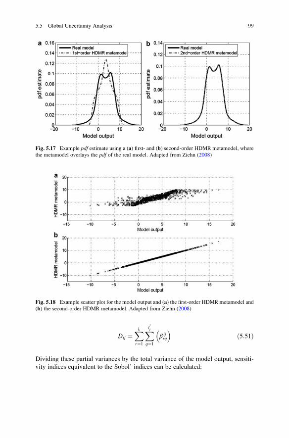
Dij ¼Xlir¼1

Xl 0jq¼1

β ijrq

ð5:51Þ

Dividing these partial variances by the total variance of the model output, sensiti-

vity indices equivalent to the Sobol’ indices can be calculated:

Fig. 5.18 Example scatter plot for the model output and (a) the first-order HDMRmetamodel and

(b) the second-order HDMR metamodel. Adapted from Ziehn (2008)

Fig. 5.17 Example pdf estimate using a (a) first- and (b) second-order HDMR metamodel, where

the metamodel overlays the pdf of the real model. Adapted from Ziehn (2008)


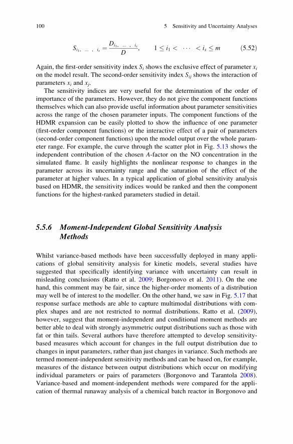
Si1, ... , is ¼Di1, ... , is

D, 1 � i1 < � � � < is � m ð5:52Þ

Again, the first-order sensitivity index Si shows the exclusive effect of parameter xion the model result. The second-order sensitivity index Sij shows the interaction of

parameters xi and xj.The sensitivity indices are very useful for the determination of the order of

importance of the parameters. However, they do not give the component functions

themselves which can also provide useful information about parameter sensitivities

across the range of the chosen parameter inputs. The component functions of the

HDMR expansion can be easily plotted to show the influence of one parameter

(first-order component functions) or the interactive effect of a pair of parameters

(second-order component functions) upon the model output over the whole param-

eter range. For example, the curve through the scatter plot in Fig. 5.13 shows the

independent contribution of the chosen A-factor on the NO concentration in the

simulated flame. It easily highlights the nonlinear response to changes in the

parameter across its uncertainty range and the saturation of the effect of the

parameter at higher values. In a typical application of global sensitivity analysis

based on HDMR, the sensitivity indices would be ranked and then the component

functions for the highest-ranked parameters studied in detail.

5.5.6 Moment-Independent Global Sensitivity AnalysisMethods

Whilst variance-based methods have been successfully deployed in many appli-

cations of global sensitivity analysis for kinetic models, several studies have

suggested that specifically identifying variance with uncertainty can result in

misleading conclusions (Ratto et al. 2009; Borgonovo et al. 2011). On the one

hand, this comment may be fair, since the higher-order moments of a distribution

may well be of interest to the modeller. On the other hand, we saw in Fig. 5.17 that

response surface methods are able to capture multimodal distributions with com-

plex shapes and are not restricted to normal distributions. Ratto et al. (2009),

however, suggest that moment-independent and conditional moment methods are

better able to deal with strongly asymmetric output distributions such as those with

fat or thin tails. Several authors have therefore attempted to develop sensitivity-

based measures which account for changes in the full output distribution due to

changes in input parameters, rather than just changes in variance. Such methods are

termed moment-independent sensitivity methods and can be based on, for example,

measures of the distance between output distributions which occur on modifying

individual parameters or pairs of parameters (Borgonovo and Tarantola 2008).

Variance-based and moment-independent methods were compared for the appli-

cation of thermal runaway analysis of a chemical batch reactor in Borgonovo and


Tarantola (2008). Different importance rankings were found depending on whether

moment-independent or variance-based techniques were used. The enthalpy of

reaction was found to influence the entire output distribution the most, whereas

its variance was most influenced by the Semenov number. However, non-important

model inputs were found to be the same in both cases. Hence, if the aim of the study

were to identify important and non-important parameters for the purpose of model

improvement, the outcome would have been the same.

5.6 Uncertainty Analysis of Gas Kinetic Models

Based on the computer simulation of detailed reaction mechanisms, information

about reaction kinetics can be used for the solution of problems in the chemical

industries, systems biology, energetics and environmental protection. An important

point is that the results of simulations may provide basic information which is not

easily available in other ways, by replacing, for example, expensive experimental

test and design programs. In environmental protection, often it may not even be

possible to perform well-defined experiments within a real-world environment, and

therefore, the assessment of the environmental impacts of strategic decisions must

be tested by running model scenarios. It is also fair to say that whilst improvements

in available computer power have allowed us to represent chemical processes

with increasing levels of model detail, our ability to accurately specify the required

high-dimensional input data often does not keep pace with the development of

model structure. A classic example of this is in combustion modelling, where the

use of automatic mechanism generation has allowed the specification of reaction

pathways for more and more complex starting molecules (e.g. low-temperature

oxidation of large hydrocarbons (Battin-Leclerc 2008)). However, the thermo-

chemical parameters for each species often have to be estimated rather than being

determined from first principles. As a result, whilst our ability to resolve complex

processes numerically appears to improve over time, our trust in the predictions of

such models may not. The evaluation of such models becomes a key task, and our

ability to improve their predictions with respect to validation data is a vital part of

model development. In all cases, the reliability of the simulation results is crucial. A

reaction kinetic model will be inaccurate if important reaction steps are missing or

if all important reaction steps are present, but their thermodynamic or kinetic

parameters are known with large uncertainty. It is also not easy to assess the effect

of adding further reaction steps. However, using the methods of sensitivity and

uncertainty analysis discussed above, the consequences of uncertainties in model

parameters can be investigated. In this section we discuss the sources of infor-

mation on parameter uncertainty and how these are quantified within gas kinetics

systems. In liquid-phase kinetics and in biological kinetic (systems biology)

models, the uncertainties of the parameters are usually not well known. However,

gas kinetic databases contain information about the uncertainty of model input

5.6 Uncertainty Analysis of Gas Kinetic Models 101

parameters, which facilitates the detailed uncertainty and sensitivity analyses

described above.

5.6.1 Uncertainty of the Rate Coefficients

Data collections containing the rate parameters of gas-phase elementary reactions

usually characterise the uncertainty of rate coefficients at a given temperature using

a single value. For combustion, pyrolysis and certain chemical engineering pro-

cesses, the temperature can be very high (e.g. up to 2,500 K), and therefore, the

uncertainty parameter is also defined across a wide range of temperatures. The

uncertainty parameter f is defined (Baulch et al. 2005) in the following way:

f ¼ log10k0

kmin

� �¼ log10

kmax

k0

� �ð5:53Þ

where k0 is the recommended (most probable or nominal) value of the rate coeffi-

cient based on an assessment of available experimental and theoretical studies, and

kmin and kmax are the extreme, but still not excludable values. According to this

assumption, the upper and lower extreme values differ from the recommended

value by a multiplication factor, which means that on a logarithmic scale, the

extreme values are positioned symmetrically around the recommended value.

Rearranging this equation yields

kmax

k0¼ 10f ð5:54Þ

or

ln kmaxf g � ln k0� � ¼ f ln10 ð5:55Þ

Theoretically one should not calculate the logarithm of a quantity with a physical

dimension; therefore, the original quantity has to be converted to a dimensionless

value. According to accepted notation (JCGM 2008), a curly bracket indicates the

specific value of a physical quantity having a given unit.

Equation (5.54) means that the rate coefficient k0 is uncertain according to a

multiplication factor u¼ 10f. Typical values of the uncertainty parameter f are 0.3,0.5 and 0.7, which means that the extreme values differ from the recommended

value by multiplication factors of 2.00, 3.16 and 5.01, respectively (see Table 5.1).

This uncertainty parameter f has been defined for a range of gas-phase systems by a

series of researchers including Warnatz (1984), Tsang and Hampson (1986), Tsang

(1992), Baulch et al. (1992, 1994, 2005) and Konnov (2008). The specification of

f allows the calculation of uncertainty ranges which may be used within the context

of the global sensitivity methods described in the previous section.


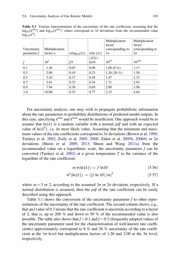
For uncertainty analysis, one may wish to propagate probabilistic information

about the rate parameters to probability distributions of predicted model outputs. In

this case, specifying kmin and kmax would be insufficient. One approach would be to

assume that ln{k} is a random variable with a normal pdf and with an expected

value of ln{k0}, i.e. its most likely value. Assuming that the minimum and maxi-

mum values of the rate coefficients correspond to 3σ deviations (Brown et al. 1999;

Turanyi et al. 2002; Zsely et al. 2005, 2008; Zador et al. 2005b, 2006b) or 2σdeviations (Sheen et al. 2009, 2013; Sheen and Wang 2011a) from the

recommended value on a logarithmic scale, the uncertainty parameter f can be

converted (Turanyi et al. 2002) at a given temperature T to the variance of the

logarithm of the rate coefficient:

m σ ln kf gð Þ ¼ f ln10 ð5:56Þσ2 ln kf gð Þ ¼ f ln 10ð Þ=mð Þ2 ð5:57Þ

where m¼ 3 or 2, according to the assumed 3σ or 2σ deviation, respectively. If a

normal distribution is assumed, then the pdf of the rate coefficient can be easily

described using this approach.

Table 5.1 shows the conversion of the uncertainty parameter f to other repre-

sentations of the uncertainty of the rate coefficient. The second column shows, e.g.,

that an f value of 0.3 means that the rate coefficient is uncertain according to a factor

of 2, that is, up to 200 % and down to 50 % of the recommended value is also

possible. The table also shows that f¼ 0.1 and f¼ 0.3 (frequently adopted values of

the uncertainty parameter used for the characterisation of well-known rate coeffi-

cients) approximately correspond to 8 % and 26 % uncertainty of the rate coeffi-

cient at the 1σ level but multiplication factors of 1.26 and 2.00 at the 3σ level,

respectively.

Table 5.1 Various representations of the uncertainty of the rate coefficient, assuming that the

log10{kmin} and log10{k

max} values correspond to 3σ deviations from the recommended value

log10{k0}

Uncertainty

parameter fMultiplication

factor u σ(log10{k}) σ(ln {k})

Multiplication

factor

corresponding to

1σ

Multiplication

factor

corresponding to

2σ

f 10f f/3( f/3)�ln10 10f/3 102f/3

0.1 1.26 0.03 0.08 1.08 (8 %) 1.17

0.3 2.00 0.10 0.23 1.26 (26 %) 1.58

0.5 3.16 0.17 0.38 1.47 2.15

0.7 5.01 0.23 0.54 1.71 2.93

0.9 7.94 0.30 0.69 2.00 3.98

1.0 10.00 0.33 0.77 2.15 4.64


Reaction kinetic data collections in atmospheric chemistry define the uncertainty

of the rate coefficient in a different way. The top of the troposphere is 7 km to 20 km

from the Earth surface (Clarke and Tomlin 1999), depending on the season and the

latitude. In the troposphere the temperature of the air is typically between �53 �Cand +47 �C (220 K� 320 K). The stratosphere is located above the troposphere

having a width of about 50 km with temperature increasing with altitude from about

�53 �C to �3 �C (220 K� 270 K). This means that all chemical reactions in the

troposphere and stratosphere occur between 220 K and 320 K. Thus, the tempera-

ture interval of atmospheric chemical reactions is much narrower than for combus-

tion reactions (300 K� 2,500 K). The rate coefficient of most atmospheric

chemical reactions has been measured at room temperature, and therefore the

uncertainty of the rate coefficient is expected to be lowest near 298 K. At higher

and lower temperatures usually fewer measurements were carried out, and therefore

the uncertainty of the rate coefficients is usually higher both above and below

298 K. For this reason atmospheric reaction kinetics data collections define the

uncertainty of the rate coefficients so that its minimum is at 298 K.

The IUPAC collections of atmospheric kinetic data (IUPAC 2014; Atkinson

et al. 2004, 2006, 2007, 2008) define the uncertainty of the rate coefficient as follows:

Δlog10 k Tð Þf g ¼ d Tð Þ ¼ d0 þ g

ln10� T�1 � T�1

0

� � ð5:58Þ

where T0¼ 298 K, the uncertainty parameter is d0¼Δ log10{ k (T0)} at tempera-

ture T0 and the parameter g characterises the uncertainty of the ratio E/R. In some

cases, Eq. (5.58) becomes ambiguous since d0 and g may take positive or negative

values. Therefore, the following modified equation was proposed by Nagy and

Turanyi (2011):

d Tð Þ ¼ d0j j þ g

ln10� T�1 � T�1

0

� �� ð5:59Þ

In the IUPAC atmospheric chemical databases, uncertainties g and d(T) of

quantities E/R and log10{k (T )}, respectively, belong to 2σ, which allows (Nagy

and Turanyi 2011) the calculation of the corresponding standard deviations:

σ log10 kf gð Þ ¼ d Tð Þ2

ð5:60Þ

σ ln kf gð Þ ¼ ln10

2d Tð Þ ð5:61Þ

σ E=Rð Þ ¼ gj j2

ð5:62Þ

The Jet Propulsion Laboratory (JPL) regularly publishes an atmospheric kinetics

and photochemistry database. Currently the latest version is number 17 that was

published in 2011 (Sander et al. 2011).


The JPL databases define the temperature dependence of uncertainty parameter

fJPL(T ) using the following equation:

f JPL Tð Þ ¼ f JPL T0ð Þ exp g T�1 � T�10

�� ð5:63Þ

where T0¼ 298 K and parameters g and fJPL(T0) are positive constants. Using the

notation fJPL,0¼ fJPL(T0), the logarithmic form of this equation is

ln f JPL Tð Þ ¼ ln f JPL,0 þ g T�1 � T�10

�� ð5:64Þ

The uncertainty parameter defined this way is also a piecewise linear function of

T� 1 and this uncertainty has a minimum at temperature T0¼ 298K. The upper and

lower limits belonging to the standard deviation (1σ) can be obtained by multiply-

ing and dividing the recommended value of the rate coefficient by the parameter

fJPL(T ), respectively:

σ ln kf gð Þ ¼ ln f JPL Tð Þ ð5:65Þ

In most uncertainty studies published so far (see e.g. Brown et al. (1999),

Turanyi et al. (2002), Zsely et al. (2005), Zador et al. (2005a, b, 2006a) and Zsely

et al. (2008)), where the uncertainties of the rate coefficients were utilised, the

uncertainty of kwas considered to be equal to the uncertainty of the pre-exponentialfactor A. This implies that the uncertainty of parameters E and n is zero, which is anunrealistic assumption. In a global sensitivity analysis study of a turbulent

reacting atmospheric plume, Ziehn et al. (2009a) demonstrated the importance of

uncertainties in E/R for the reaction NO+O3¼NO2+O2. In this case for the

prediction of mean plume centre line O3 concentrations, the sensitivity to the

assumed value for E/R was almost a factor of 20 higher than that of the A-factor,based on input parameter uncertainty factors provided by the evaluation of

Androulakis (2004, 2004). However, in this case the parameters of the Arrhenius

expression for the chemical reactions considered were allowed to vary indepen-

dently. In fact, the characterisation of the joint uncertainty of the Arrhenius

parameters is important for the realistic calculation of the uncertainty of chemical

kinetic simulation results as will be discussed in the next section.

A particularly interesting area of kinetic modelling and sensitivity analysis is

that of the chemistry of extraterrestrial atmospheres. The atmosphere of Titan, the

largest moon of Saturn, represents a particularly challenging environment since it

encompasses a low-temperature range of 50–200 K. The uncertainties in rate

coefficients measured at room temperature can therefore be exaggerated when

extrapolated to such low temperatures. As pointed out in Hebrard et al. (2009),

state-of-the-art photochemical models of Titan’s atmosphere may contain less than

10 % of reactions where the rate coefficients have been measured in the relevant

temperature range. The reaction mechanisms of the chemical transformations in the

atmosphere of Titan have been the subject of many uncertainty studies (Carrasco

and Pernot 2007, Carrasco et al. 2007, 2008a, b; Dobrijevic et al. 2008, 2010;


Hebrard et al. 2009; Peng et al. 2010; Plessis et al. 2010). Hebrard et al. (2009), for

example, highlight those reactions for which an improvement in low-T rate constant

precision is likely to produce improvements within models of Titan’s atmosphere.

Photolysis reactions of the major species were identified as a limiting factor in

improving model accuracy.

Another important problem in the atmospheric chemistry models of Titan is the

handling of the uncertainty of reaction branching ratios. This can be an important

issue for the uncertainty analysis of many other reaction kinetic models. Chemical

kinetic databases provide the uncertainty of rate coefficients independently of each

other. Yet, for multichannel reactions using a direct method, it is easier to measure

the overall rate coefficient than the rate coefficients of the constituent reaction steps.

The branching ratios are then determined in other measurements. However, it is

important to note that the branching ratios are correlated, since their sum has a unit

value. Carrasco et al. (Carrasco and Pernot 2007; Plessis et al. 2010) demonstrated

that the correlated branching ratios follow a Dirichlet distribution. The method

was applied to the case of Titan ionospheric chemistry and used for the estimation

of the effect of branching ratio correlations on the uncertainty of calculated

concentrations.

5.6.2 Characterisation of the Uncertainty of the ArrheniusParameters

In this section, the relationship between the temperature dependence of the uncer-

tainty of the rate coefficient and the joint pdf of the Arrhenius parameters is

discussed based primarily on Nagy and Turanyi (2011, 2012). As was mentioned

in Sect. 2.2.1, the temperature dependence of the rate coefficient k can be describedby the modified Arrhenius equation k¼ATn exp(�E/RT). Introducing the

transformed parameters κ¼ ln {k}, α¼ ln{A} and ε¼E/R, the linearised form of

the modified Arrhenius equation is

κ Tð Þ ¼ αþ n � ln Tf g � ε � T�1 ð5:66Þ

As above, curly bracket {.} means the dimensionless value of the quantity given in

the bracket.

The other generally used function is the (original) Arrhenius equation k¼A exp

(�E/RT) with the linearised form

κ Tð Þ ¼ α� ε � T�1 ð5:67Þ

Usually gas kinetics data collections suggest not only the Arrhenius parameters

but also parameters that characterise the uncertainty of the rate coefficients at given

temperatures as discussed in the previous section. The temperature interval [T1,T2],



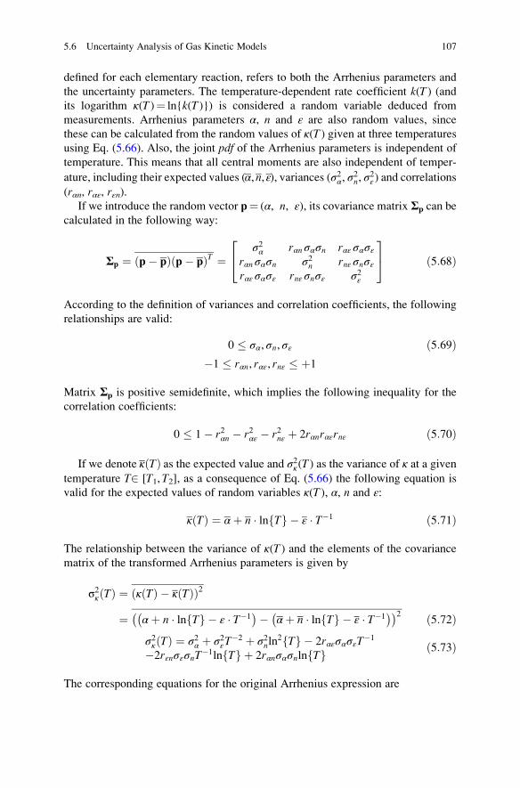
defined for each elementary reaction, refers to both the Arrhenius parameters and

the uncertainty parameters. The temperature-dependent rate coefficient k(T ) (andits logarithm κ(T )¼ ln{k(T)}) is considered a random variable deduced from

measurements. Arrhenius parameters α, n and ε are also random values, since

these can be calculated from the random values of κ(T ) given at three temperatures

using Eq. (5.66). Also, the joint pdf of the Arrhenius parameters is independent of

temperature. This means that all central moments are also independent of temper-

ature, including their expected values (α,n,ε), variances (σ2α, σ2n, σ

2ε) and correlations

(rαn, rαε, rεn).If we introduce the random vector p¼ (α, n, ε), its covariance matrix Σp can be

calculated in the following way:

Σp ¼ p� pð Þ p� pð ÞT ¼σ2α rαn σασn rαε σασε

rαn σασn σ2n rnε σnσεrαε σασε rnε σnσε σ2ε

24 35 ð5:68Þ

According to the definition of variances and correlation coefficients, the following

relationships are valid:

0 � σα, σn, σε ð5:69Þ�1 � rαn, rαε, rnε � þ1

Matrix Σp is positive semidefinite, which implies the following inequality for the

correlation coefficients:

0 � 1� r2αn � r2αε � r2nε þ 2rαnrαεrnε ð5:70Þ

If we denote κ Tð Þ as the expected value and σ2κ(T) as the variance of κ at a giventemperature T2 [T1, T2], as a consequence of Eq. (5.66) the following equation is

valid for the expected values of random variables κ(T ), α, n and ε:

κ Tð Þ ¼ αþ n � ln Tf g � ε � T�1 ð5:71Þ

The relationship between the variance of κ(T ) and the elements of the covariance

matrix of the transformed Arrhenius parameters is given by

σ2κ Tð Þ ¼ κ Tð Þ � κ Tð Þð Þ2

¼ αþ n � ln Tf g � ε � T�1� �� αþ n � ln Tf g � ε � T�1

� �� 2 ð5:72Þσ2κ Tð Þ ¼ σ2α þ σ2εT

�2 þ σ2nln2 Tf g � 2rαεσασεT

�1

�2rεnσεσnT�1ln Tf g þ 2rαnσασnln Tf g ð5:73Þ

The corresponding equations for the original Arrhenius expression are


σ2κ Tð Þ ¼ κ Tð Þ � κ Tð Þð Þ2 ¼ α� ε � T�1� �� α� ε � T�1

� �� 2 ð5:74Þσ2κ Tð Þ ¼ σ2α þ σ2εT

�2 � 2rαεσασεT�1 ð5:75Þ

A similar expression to (5.75) has been derived by Hebrard et al. (2009).

It is commonly assumed that the pdf of κ(T ) is normally distributed at each

temperature, truncated at m � σκ(T ) (m¼ 2 or 3). The corresponding equation is

g1 κ; Tð Þ ¼ 1ffiffiffiffiffiffi2π

pσκ Tð Þ exp �

κ Tð Þ � κ Tð Þ 2

2σ2κ Tð Þ

264375 ð5:76Þ

If the pdf of κ(T) has a normal distribution at each temperature, then the joint pdfof the transformed Arrhenius parameters is a multidimensional normal distribution

(Nagy and Turanyi 2011) (some restrictions for the correlation of the κ(T ) valuesalso have to be fulfilled). The following equation defines the 3D normal distribution

of Arrhenius parameters p¼ (α, n, ε), parameterised using the expected value p and

the covariance matrix Σp:

gN pð Þ ¼ 1

2πð ÞN=2 ffiffiffiffiffiffiffiffiffiffiffiffidetΣp

p exp �1

2p� pð ÞTΣ�1

p p� pð Þ� �

ð5:77Þ

where N¼ 3 is the number of parameters.

According to the usual handling of uncertainties in rate coefficients, their values

have to remain between kmin and kmax at each temperature. This means that the joint

pdf of the Arrhenius parameters has to be truncated so that the calculated κ(T )remains between the uncertainty limits for any temperature T within the interval

[T1,T2]:

κ� κ Tð Þj j � m � σκ Tð Þ ð5:78Þ

For atmospheric chemical reactions, m¼ 2 is usually assumed and thus 95 % of

the κ(T ) values (calculated from the untruncated pdf) remain within the interval

(kmin, kmax) when assuming a normal distribution for κ(T ). Most authors assume that

for combustion reactions m¼ 3, and in this case 99.7 % of the randomly selected

values are within the uncertainty interval (kmin, kmax) and only 0.3 % are outside

it. The integral of the pdf over the whole space of events is equal to one. Using the

truncations above, only a small part of the pdf is cut off, and therefore, the

normalisation of the pdf is not changed significantly. The elements of the covari-

ance matrix of parameters (α, n, ε) are also not changed significantly.

The covariance matrix of the three parameters of the modified Arrhenius equa-

tion contains six parameters. To determine these parameters, the uncertainty of the

rate coefficient has to be known for at least six different temperatures. Fitting these

parameters requires not only Eq. (5.73) but also expressions (5.69) and (5.70)


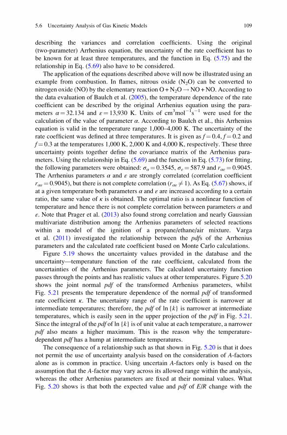
describing the variances and correlation coefficients. Using the original

(two-parameter) Arrhenius equation, the uncertainty of the rate coefficient has to

be known for at least three temperatures, and the function in Eq. (5.75) and the

relationship in Eq. (5.69) also have to be considered.

The application of the equations described above will now be illustrated using an

example from combustion. In flames, nitrous oxide (N2O) can be converted to

nitrogen oxide (NO) by the elementary reaction O+N2O!NO+NO. According to

the data evaluation of Baulch et al. (2005), the temperature dependence of the rate

coefficient can be described by the original Arrhenius equation using the para-

meters α¼ 32.134 and ε¼ 13,930 K. Units of cm3mol�1s�1 were used for the

calculation of the value of parameter α. According to Baulch et al., this Arrhenius

equation is valid in the temperature range 1,000–4,000 K. The uncertainty of the

rate coefficient was defined at three temperatures. It is given as f¼ 0.4, f¼ 0.2 and

f¼ 0.3 at the temperatures 1,000 K, 2,000 K and 4,000 K, respectively. These three

uncertainty points together define the covariance matrix of the Arrhenius para-

meters. Using the relationship in Eq. (5.69) and the function in Eq. (5.73) for fitting,

the following parameters were obtained: σα¼ 0.3545, σε¼ 587.9 and rαε¼ 0.9045.

The Arrhenius parameters α and ε are strongly correlated (correlation coefficient

rαε¼ 0.9045), but there is not complete correlation (rαε 6¼ 1). As Eq. (5.67) shows, if

at a given temperature both parameters α and ε are increased according to a certainratio, the same value of κ is obtained. The optimal ratio is a nonlinear function of

temperature and hence there is not complete correlation between parameters α and

ε. Note that Prager et al. (2013) also found strong correlation and nearly Gaussian

multivariate distribution among the Arrhenius parameters of selected reactions

within a model of the ignition of a propane/ethane/air mixture. Varga

et al. (2011) investigated the relationship between the pdfs of the Arrhenius

parameters and the calculated rate coefficient based on Monte Carlo calculations.

Figure 5.19 shows the uncertainty values provided in the database and the

uncertainty—temperature function of the rate coefficient, calculated from the

uncertainties of the Arrhenius parameters. The calculated uncertainty function

passes through the points and has realistic values at other temperatures. Figure 5.20

shows the joint normal pdf of the transformed Arrhenius parameters, whilst

Fig. 5.21 presents the temperature dependence of the normal pdf of transformed

rate coefficient κ. The uncertainty range of the rate coefficient is narrower at

intermediate temperatures; therefore, the pdf of ln {k} is narrower at intermediate

temperatures, which is easily seen in the upper projection of the pdf in Fig. 5.21.

Since the integral of the pdf of ln {k} is of unit value at each temperature, a narrower

pdf also means a higher maximum. This is the reason why the temperature-

dependent pdf has a hump at intermediate temperatures.

The consequence of a relationship such as that shown in Fig. 5.20 is that it does

not permit the use of uncertainty analysis based on the consideration of A-factorsalone as is common in practice. Using uncertain A-factors only is based on the

assumption that the A-factor may vary across its allowed range within the analysis,

whereas the other Arrhenius parameters are fixed at their nominal values. What

Fig. 5.20 shows is that both the expected value and pdf of E/R change with the


Fig. 5.19 The rate coefficient of reaction O+N2O!NO+NO changes with temperature

according to the original (2-parameter) Arrhenius equation, and its uncertainty parameter f isknown at temperatures 1,000 K, 2,000 K and 4,000 K (circles). The line shows the temperature

dependence of the uncertainty parameter, calculated from the assumed probability density function

of modified Arrhenius parameters α¼ ln{A} and ε¼E/R (Nagy and Turanyi 2011)

Fig. 5.20 The joint pdf of normal distribution of the modified Arrhenius parameters belonging to

the function f(T ) presented in Fig. 5.19. It is clear that there is a strong correlation between

parameters α¼ ln{A} and ε¼E/R (Nagy and Turanyi 2011)


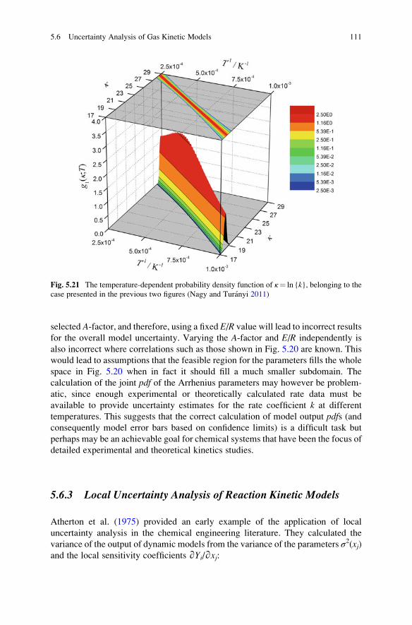
selected A-factor, and therefore, using a fixed E/R value will lead to incorrect results

for the overall model uncertainty. Varying the A-factor and E/R independently is

also incorrect where correlations such as those shown in Fig. 5.20 are known. This

would lead to assumptions that the feasible region for the parameters fills the whole

space in Fig. 5.20 when in fact it should fill a much smaller subdomain. The

calculation of the joint pdf of the Arrhenius parameters may however be problem-

atic, since enough experimental or theoretically calculated rate data must be

available to provide uncertainty estimates for the rate coefficient k at different

temperatures. This suggests that the correct calculation of model output pdfs (andconsequently model error bars based on confidence limits) is a difficult task but

perhaps may be an achievable goal for chemical systems that have been the focus of

detailed experimental and theoretical kinetics studies.

5.6.3 Local Uncertainty Analysis of Reaction Kinetic Models

Atherton et al. (1975) provided an early example of the application of local

uncertainty analysis in the chemical engineering literature. They calculated the

variance of the output of dynamic models from the variance of the parameters σ2(xj)and the local sensitivity coefficients ∂Yi/∂xj:

Fig. 5.21 The temperature-dependent probability density function of κ¼ ln {k}, belonging to the

case presented in the previous two figures (Nagy and Turanyi 2011)


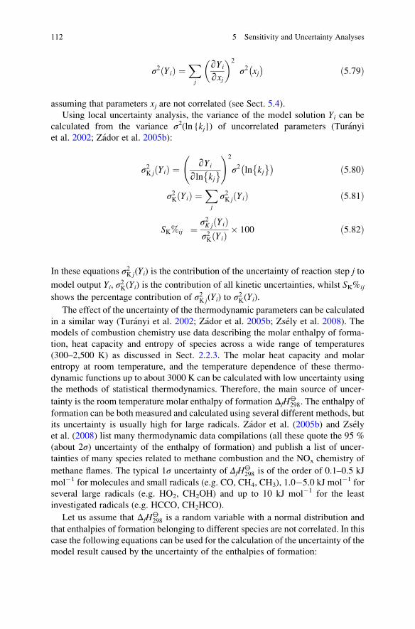
σ2 Yið Þ ¼Xj

∂Yi

∂xj

� �2

σ2 xj� � ð5:79Þ

assuming that parameters xj are not correlated (see Sect. 5.4).

Using local uncertainty analysis, the variance of the model solution Yi can be

calculated from the variance σ2(ln {kj}) of uncorrelated parameters (Turanyi

et al. 2002; Zador et al. 2005b):

σ2K j Yið Þ ¼ ∂Yi

∂ln kj� � !2

σ2 ln kj� �� ð5:80Þ

σ2K Yið Þ ¼Xj

σ2K j Yið Þ ð5:81Þ

SK%ij ¼ σ2K j Yið Þσ2K Yið Þ � 100 ð5:82Þ

In these equations σ2K j(Yi) is the contribution of the uncertainty of reaction step j to

model output Yi, σ2K(Yi) is the contribution of all kinetic uncertainties, whilst SK%ij

shows the percentage contribution of σ2K j(Yi) to σ2K(Yi).

The effect of the uncertainty of the thermodynamic parameters can be calculated

in a similar way (Turanyi et al. 2002; Zador et al. 2005b; Zsely et al. 2008). The

models of combustion chemistry use data describing the molar enthalpy of forma-

tion, heat capacity and entropy of species across a wide range of temperatures

(300–2,500 K) as discussed in Sect. 2.2.3. The molar heat capacity and molar

entropy at room temperature, and the temperature dependence of these thermo-

dynamic functions up to about 3000 K can be calculated with low uncertainty using

the methods of statistical thermodynamics. Therefore, the main source of uncer-

tainty is the room temperature molar enthalpy of formation ΔfH⦵298. The enthalpy of

formation can be both measured and calculated using several different methods, but

its uncertainty is usually high for large radicals. Zador et al. (2005b) and Zsely

et al. (2008) list many thermodynamic data compilations (all these quote the 95 %

(about 2σ) uncertainty of the enthalpy of formation) and publish a list of uncer-

tainties of many species related to methane combustion and the NOx chemistry of

methane flames. The typical 1σ uncertainty of ΔfH⦵298 is of the order of 0.1–0.5 kJ

mol�1 for molecules and small radicals (e.g. CO, CH4, CH3), 1.0�5.0 kJ mol�1 for

several large radicals (e.g. HO2, CH2OH) and up to 10 kJ mol�1 for the least

investigated radicals (e.g. HCCO, CH2HCO).

Let us assume that ΔfH⦵298 is a random variable with a normal distribution and

that enthalpies of formation belonging to different species are not correlated. In this

case the following equations can be used for the calculation of the uncertainty of the

model result caused by the uncertainty of the enthalpies of formation:



σ2T j Yið Þ ¼ ∂Yi

∂Δf H⦵298 jð Þ

� �2

σ2 Δf H⦵298 jð Þ� � ð5:83Þ

σ2T Yið Þ ¼Xj

σ2T j Yið Þ ð5:84Þ

ST%ij ¼ σ2T j Yið Þσ2T Yið Þ � 100 ð5:85Þ

where σ2T j(Yi) is the contribution of the uncertainty of the j-th thermodynamic

parameter to the variance of model output, Yi, σ2T(Yi) is the contribution of the

uncertainty of all thermodynamic parameters, whilst ST%ij shows the percentage

contribution of σ2T j(Yi) to σ2T(Yi).

In most reaction mechanisms that are expressed in reversible form, the forward

rate coefficients have not been used for the derivation of the enthalpies of forma-

tion; therefore, the kinetic and thermodynamic data can be considered as

uncorrelated. In this case the variance of model result Yi can be obtained as the

sum of the variances of the kinetic and thermodynamic parameters:

σ2 Yið Þ ¼ σ2K Yið Þ þ σ2T Yið Þ ð5:86Þ

The effects of the kinetic and thermodynamic parameters can be compared by

using the following unified parameter vector: x¼ [ln {k1}, ln {k2}, . . . , ln kNRf g,

ΔfH⦵298 (1), ΔfH

⦵298 (2), . . ., ΔfH

⦵298 (NS)], which includes the logarithms of the rate

coefficients of NR reaction steps and the room temperature enthalpies of formation

of NS species. σ2j (Yi) denotes the contribution of parameter xj (which is either kinetic

or thermodynamic) to the variance of model output Yi. The quantity S%ij shows the

percentage contribution of σ2j (Yi) to the overall variance σ2(Yi):

S%ij ¼σ2j Yið Þσ2 Yið Þ � 100 ð5:87Þ

In this way, for a reaction mechanism containing only reversible reaction steps, the

fraction of the uncertainties originating from the kinetic and thermodynamic

parameters can be compared within the overall uncertainty analysis of the model

results.

Note, that typical thermodynamic databases contain the uncertainties of the

enthalpies of formation of the species separately and do not provide information

about correlation of these uncertainties. The Active Thermochemical Table (ATcT)

approach (Ruscic et al. 2004, 2005, 2006, 2014; Ruscic ; Stevens et al. 2010; Ruscic

2013, 2014) takes into account that many measurements contain information for the

thermodynamic data of several species together, and therefore the determination of

the thermodynamic data from all available experimental measurements and theo-

retical calculations has to occur in a single step. This approach makes the


determined thermodynamic data more accurate and more consistent, and also

allows the calculation of the joint uncertainties. A similar approach, called Network

of Computed Reaction Enthalpies to Atom-Based Thermochemistry (NEAT), was

suggested by Csaszar and Furtenbacher (2010). The NEAT approach is restricted to

theoretically calculated thermochemical data, and it combines the joint determina-

tion of the enthalpies of formation of species with the fact that the enthalpies of

formation correspond to the total atomisation energies of the species. The NEAT

calculations also provide correlated uncertainties.

5.6.4 Examples of the Application of Uncertainty Analysisto Methane Flame Models

One of the most important fuels is natural gas, mainly consisting of methane (CH4).

Hence, the combustion of methane is of central importance, and the development

and evaluation of kinetic mechanisms describing methane oxidation has been a key

task of the combustion research community. Often simple experimental setups are

used for kinetic model evaluation, where the physics that may be involved in more

complex flows is of lower importance. The most frequently investigated methane

flame is a laminar, stationary flame in which the cold methane–air mixture is at

atmospheric pressure (1 atm) and room temperature (25 �C). The simplest case is

the simulation of a flame where the temperature and concentrations depend only on

the distance from the flame front. Such flames are commonly used in laboratory

studies and are called flat flames. Their advantage is that such flames can be

modelled using one spatial dimension, allowing detailed chemical kinetics to be

included within the model without excessive computational cost (e.g. Marinov

et al. (1996)). The combustion of methane can be quantitatively described by

reaction mechanisms including several hundred reaction steps. One example of

such a mechanism is the Leeds Methane Oxidation Mechanism (Hughes

et al. 2001b) that contains 175 reversible reaction steps. The reader should refer

to Sect. 2.2.3 for a discussion of the calculation of reverse rate coefficients.

This methane oxidation mechanism was investigated by Turanyi et al. (2002)

and Zador et al. (2005b) using several methods of uncertainty analysis. Later Zsely

et al. (2008) extended the investigations to the production of NO during methane

combustion and Ziehn et al. to the interaction of sulphur- and nitrogen-containing

compounds within a methane flame (Ziehn and Tomlin 2008b). In the study of

Turanyi et al., an uncertainty parameter fwas assigned to each forward reaction ratecoefficient of the methane oxidation mechanism. This parameter was considered to

be temperature independent, and therefore σ2(ln {k}) was identical to σ2(ln {A}).The standard deviations of the molar enthalpies of formation of all species were

also collected from thermodynamic databases.

The overall reaction equation shows the ratio of fuel and oxidiser needed for a

complete reaction. This ratio (nfuel/nox)st is called the stoichiometric ratio. The



equivalence ratio ϕ, defined by the equation below, shows the deviation of the

actual mixture composition nfuel/nox from the stoichiometric mixture:

ϕ ¼ nfuel=noxnfuel=noxð Þst

ð5:88Þ

Fuel–oxidiser mixtures having equivalence ratio ϕ< 1 and ϕ> 1 are called fuel

lean and fuel rich, respectively. Usually the important reactions are different at the

combustion of lean and rich mixtures.

Using the program PREMIX (Kee et al. 1985), premixed, stationary, laminar,

one-dimensional methane–air flames were simulated. The cold mixture boundary

conditions were p¼ 1 atm and T¼ 298.15 K. The calculations were carried out for

lean (ϕ¼ 0.70), stoichiometric (ϕ¼ 1.00) and rich (ϕ¼ 1.20) equivalence ratios.

PREMIX calculated not only the concentration� distance curves, but also normed

sensitivities ∂lnYi/∂ ln kj, and the sensitivities of the calculated concentrations withrespect to the enthalpies of formation of species.

The target model outputs under investigation were the laminar flame velocity vL,the maximum adiabatic flame temperature Tmax and the maximum concentrations

of species H, O, OH, CH and CH2. The laminar flame velocity is a frequently

investigated global feature of combustion (Bosschaart and de Goey 2003). For

example, in an internal combustion engine the flame velocity is a measure of the

fuels ability to undergo controlled combustion. The accurate calculation of the

flame temperature is also very important, because one of the aims of the flame

calculations is the determination of heat production. Together, the flame velocity

and adiabatic flame temperature are important properties which indicate the poten-

tial combustion efficiency within an engine and hence the ability of a chemical

mechanism to accurately predict these properties is important for its use within

engine design models. In addition, temperature has a strong influence on the rates of

the chemical processes occurring within the flame. The most effective chain carrier

during the combustion of hydrocarbons is the H-atom. Therefore, the accurate

calculation of its concentration is very important. One of the usual aims of natural

gas combustion simulations is finding conditions with minimal NO production,

since emissions of NO from combustion devices to the atmosphere contribute to a

range of environmental impacts including acid deposition and smog formation

(Clarke and Tomlin 1999). For methane flames, NO production typically depends

on temperature and the concentrations of species H, O, OH, CH and CH2, since the

major NO production pathways include thermal NO generation (main reaction

N2 +O!NO+N) and prompt NO generation (main reaction N2 +CH!NCN

+H). The production pathways for NO are briefly summarised in the article of

Zsely et al. (2008).

The standard deviations of the model results were calculated using local uncer-

tainty analysis as well as via Monte Carlo analysis with Latin hypercube sampling.

For the Monte Carlo analysis, the parameters were assumed to be independent

random variables with normal distributions. More precisely, truncated normal


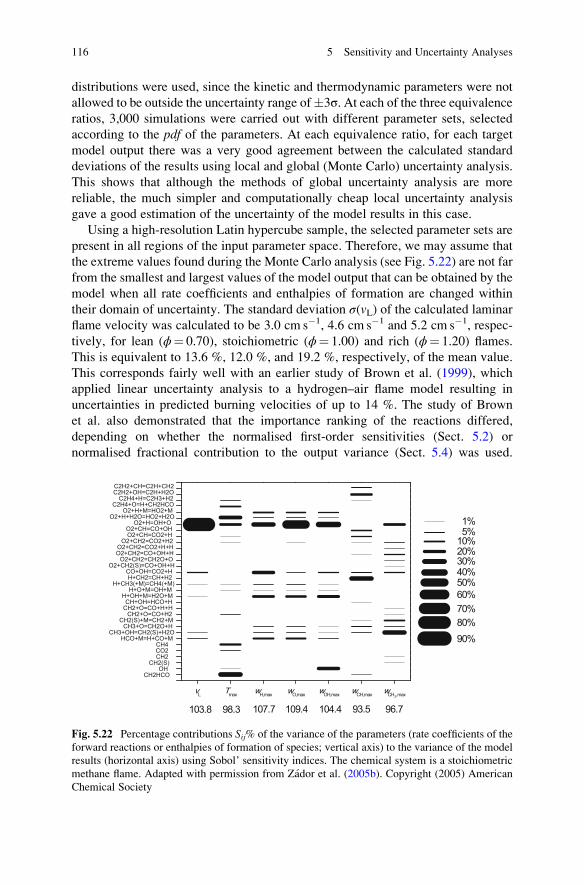
distributions were used, since the kinetic and thermodynamic parameters were not

allowed to be outside the uncertainty range of3σ. At each of the three equivalenceratios, 3,000 simulations were carried out with different parameter sets, selected

according to the pdf of the parameters. At each equivalence ratio, for each target

model output there was a very good agreement between the calculated standard

deviations of the results using local and global (Monte Carlo) uncertainty analysis.

This shows that although the methods of global uncertainty analysis are more

reliable, the much simpler and computationally cheap local uncertainty analysis

gave a good estimation of the uncertainty of the model results in this case.

Using a high-resolution Latin hypercube sample, the selected parameter sets are

present in all regions of the input parameter space. Therefore, we may assume that

the extreme values found during the Monte Carlo analysis (see Fig. 5.22) are not far

from the smallest and largest values of the model output that can be obtained by the

model when all rate coefficients and enthalpies of formation are changed within

their domain of uncertainty. The standard deviation σ(vL) of the calculated laminar

flame velocity was calculated to be 3.0 cm s�1, 4.6 cm s�1 and 5.2 cm s�1, respec-

tively, for lean (ϕ¼ 0.70), stoichiometric (ϕ¼ 1.00) and rich (ϕ¼ 1.20) flames.

This is equivalent to 13.6 %, 12.0 %, and 19.2 %, respectively, of the mean value.

This corresponds fairly well with an earlier study of Brown et al. (1999), which

applied linear uncertainty analysis to a hydrogen–air flame model resulting in

uncertainties in predicted burning velocities of up to 14 %. The study of Brown

et al. also demonstrated that the importance ranking of the reactions differed,

depending on whether the normalised first-order sensitivities (Sect. 5.2) or

normalised fractional contribution to the output variance (Sect. 5.4) was used.

vL Tmax wH,max wO,max wOH,max wCH,max wCH2,max

CH2HCOOH

CH2(S)CH2CO2CH4

HCO+M=H+CO+MCH3+OH=CH2(S)+H2O

CH3+O=CH2O+HCH2(S)+M=CH2+M

CH2+O=CO+H2CH2+O=CO+H+HCH+OH=HCO+H

H+OH+M=H2O+MH+O+M=OH+M

H+CH3(+M)=CH4(+M)H+CH2=CH+H2

CO+OH=CO2+HO2+CH2(S)=CO+OH+H

O2+CH2=CH2O+OO2+CH2=CO+OH+HO2+CH2=CO2+H+H

O2+CH2=CO2+H2O2+CH=CO2+HO2+CH=CO+OH

O2+H=OH+OO2+H+H2O=HO2+H2O

O2+H+M=HO2+MC2H4+O=H+CH2HCO

C2H4+H=C2H3+H2C2H2+OH=C2H+H2OC2H2+CH=C2H+CH2

96.793.5104.4109.4107.798.3103.8

60%50%40%30%20%10%5%1%

90%

70%80%

Fig. 5.22 Percentage contributions Sij% of the variance of the parameters (rate coefficients of the

forward reactions or enthalpies of formation of species; vertical axis) to the variance of the model

results (horizontal axis) using Sobol’ sensitivity indices. The chemical system is a stoichiometric

methane flame. Adapted with permission from Zador et al. (2005b). Copyright (2005) American

Chemical Society


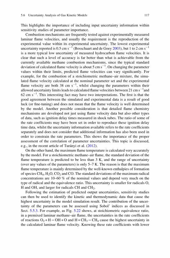
This highlights the importance of including input uncertainty information within

sensitivity studies of parameter importance.

Combustion mechanisms are frequently tested against experimentally measured

laminar flame velocities, and usually the requirement is the reproduction of the

experimental value within its experimental uncertainty. The lowest experimental

uncertainty reported is 0.5 cm s�1 (Bosschaart and de Goey 2003), but 1 to 2 cm s�1

is a more typical low uncertainty of measured hydrocarbon flame velocities. It is

clear that such a level of accuracy is far better than what is achievable from the

currently available methane combustion mechanisms, since the typical standard

deviation of calculated flame velocity is about 5 cm s�1. On changing the parameter

values within their limits, predicted flame velocities can vary significantly. For

example, for the combustion of a stoichiometric methane–air mixture, the simu-

lated flame velocity calculated at the nominal parameter set and the experimental

flame velocity are both 38 cm s�1, whilst changing the parameters within their

allowed uncertainty limits leads to calculated flame velocities between 21 cm s�1and

62 cm s�1. This interesting fact may have two interpretations. The first is that the

good agreement between the simulated and experimental data is a result of good

luck (or fine-tuning) and does not mean that the flame velocity is well determined

by the model. Another possible consideration is that detailed flame chemistry

mechanisms are developed not just using flame velocity data but also other types

of data, such as ignition delay times measured in shock tubes. The ratio of some of

the rate coefficients may have been set in order to reproduce these ignition delay

time data, whilst the uncertainty information available refers to the rate coefficients

separately and does not consider that additional information has also been used in

order to constrain the rate parameters. This shows the importance of the proper

assessment of the correlation of parameter uncertainties. This topic is discussed,

e.g., in the recent article of Turanyi et al. (2012).

On the other hand, the maximum flame temperature is calculated very accurately

by the model. For a stoichiometric methane–air flame, the standard deviation of the

flame temperature is predicted to be less than 3 K, and the range of uncertainty

(over any values of the parameters) is only 5–7 K. The reason is that the maximum

flame temperature is mainly determined by the well-known enthalpies of formation

of species CH4, H2O, CO2 and CO. The standard deviations of the maximum radical

concentrations are 10–60 % of the nominal values and depend very much on the

type of radical and the equivalence ratio. This uncertainty is smaller for radicals O,

H and OH, and larger for radicals CH and CH2.

Following the estimation of predicted output uncertainties, sensitivity studies

can then be used to identify the kinetic and thermodynamic data that cause the

highest uncertainty in the model simulation result. The contribution of the uncer-

tainty of the parameters can be assessed using Sobol’ indices as discussed in

Sect. 5.5.3. For example, as Fig. 5.22 shows, at stoichiometric equivalence ratio,

in a premixed laminar methane–air flame, the uncertainties in the rate coefficients

of reactions O2 +H¼OH+O and H+CH3¼CH4 cause the highest uncertainty in

the calculated laminar flame velocity. Knowing these rate coefficients with lower


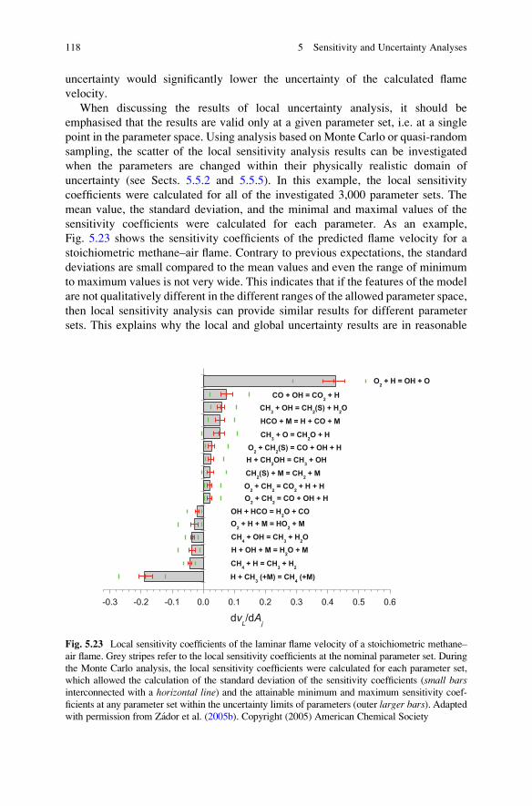
uncertainty would significantly lower the uncertainty of the calculated flame

velocity.

When discussing the results of local uncertainty analysis, it should be

emphasised that the results are valid only at a given parameter set, i.e. at a single

point in the parameter space. Using analysis based on Monte Carlo or quasi-random

sampling, the scatter of the local sensitivity analysis results can be investigated

when the parameters are changed within their physically realistic domain of

uncertainty (see Sects. 5.5.2 and 5.5.5). In this example, the local sensitivity

coefficients were calculated for all of the investigated 3,000 parameter sets. The

mean value, the standard deviation, and the minimal and maximal values of the

sensitivity coefficients were calculated for each parameter. As an example,

Fig. 5.23 shows the sensitivity coefficients of the predicted flame velocity for a

stoichiometric methane–air flame. Contrary to previous expectations, the standard

deviations are small compared to the mean values and even the range of minimum

to maximum values is not very wide. This indicates that if the features of the model

are not qualitatively different in the different ranges of the allowed parameter space,

then local sensitivity analysis can provide similar results for different parameter

sets. This explains why the local and global uncertainty results are in reasonable

-0.3 -0.2 -0.1 0.0 0.1 0.2 0.3 0.4 0.5 0.6

H + CH3 (+M) = CH4 (+M)

CH4 + H = CH3 + H2

H + OH + M = H2O + MCH4 + OH = CH3 + H2O

O2 + H + M = HO2 + MOH + HCO = H2O + CO

O2 + CH2 = CO + OH + HO2 + CH2 = CO2 + H + HCH2(S) + M = CH2 + M

H + CH2OH = CH3 + OHO2 + CH2(S) = CO + OH + H

CH3 + O = CH2O + H

HCO + M = H + CO + M

CH3 + OH = CH2(S) + H2OCO + OH = CO2 + H

O2 + H = OH + O

dvL/dA

j

Fig. 5.23 Local sensitivity coefficients of the laminar flame velocity of a stoichiometric methane–

air flame. Grey stripes refer to the local sensitivity coefficients at the nominal parameter set. During

the Monte Carlo analysis, the local sensitivity coefficients were calculated for each parameter set,

which allowed the calculation of the standard deviation of the sensitivity coefficients (small barsinterconnected with a horizontal line) and the attainable minimum and maximum sensitivity coef-

ficients at any parameter set within the uncertainty limits of parameters (outer larger bars). Adaptedwith permission from Zador et al. (2005b). Copyright (2005) American Chemical Society


agreement for this particular example. However, this is not always the case as will

be discussed in relation to further examples.

5.6.5 Applications of Response Surface Techniquesto Uncertainty Analysis in Gas Kinetic Models

In Ziehn and Tomlin (2008b) RS-HDMR methods were applied for the global

sensitivity analysis of a model of a one-dimensional low-pressure premixed meth-

ane flame used to investigate the influence of fuel sulphur and nitrogen on the NO

concentration within the burnt gas region. PREMIX was again used for the simu-

lations, with uncertainties in the parameterisation of forward rate coefficients and

thermodynamic data considered. This led to a study of 176 input parameters

(153 reaction rates and 23 enthalpies of formation) with the aim of determining

their relative importance in driving the output uncertainty in predicted [NO]. Full

details of the model scenario can be found in Tomlin (2006) with the focus here on

the fuel-rich scenario with equivalence ratio of ϕ¼ 1.6 with 0.5 % of SO2 and 1.3 %

of NH3 added to the flame. The doping with sulphur- and nitrogen-containing

compounds was designed to mimic the levels that may be found within fuels. In

this case, the mechanism using the nominal parameter values tends to overpredict

the relative increase in the NO mole fractions at the end of the flame on the addition

of SO2, compared to the experiments of Hughes et al. (2001a). The case study is

summarised here since it highlights important points relating to the evaluation of

kinetic mechanisms and to the use of local sensitivity coefficients.

In the study, the reactions were treated as reversible, with reverse rates calcu-

lated from the appropriate equilibrium constants based on enthalpies of formation

(ΔfH⦵) calculated using NASA polynomials (see Sect. 2.2.3). Because so many of

the input parameters were estimated, derived from a low number of measurements

or from single theoretical studies, the input distributions were considered to be

uniform between predefined minimum and maximum values (Tomlin 2006).

Uncertainties in the rate coefficients were expressed using A-factors only, since

for most reactions, there was insufficient information to determine the joint pdfs ofthe Arrhenius parameters.

For 176 input parameters, the full second-order HDMR expansion consists of

15,577 component functions (1 zeroth-order term + 176 first-order terms + 15,400

second-order terms). However, using a threshold of 1 % for the first- and second-

order component functions, only five of the 176 first-order component functions

and none of the 15,400 second-order component functions were approximated by

optimal-order polynomials. The resulting first-order HDMR metamodel gave

99.05 % of the tested samples within the 5 % RE (relative error) range (see

Eq. (5.49)) compared to a sample of 2,000 full model runs. This suggests that

despite the high-dimensionality of the input space of the model, the predicted NO



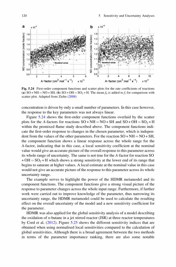
concentration is driven by only a small number of parameters. In this case however,

the response to the key parameters was not always linear.

Figure 5.24 shows the first-order component functions overlaid by the scatter

plots for the A-factors for reactions SO+NH¼NO+SH and SO+OH¼ SO2 +H

within the premixed flame study described above. The component functions indi-

cate the first-order response to changes in the chosen parameter, which is indepen-

dent from the values of the other parameters. For the reaction SO+NH¼NO+SH,

the component function shows a linear response across the whole range for the

A-factor, indicating that in this case, a local sensitivity coefficient at the nominal

value would give an accurate picture of the overall response to this parameter across

its whole range of uncertainty. The same is not true for the A-factor for reaction SO+OH¼ SO2 +H which shows a strong sensitivity at the lower end of its range that

begins to saturate at higher values. A local estimate at the nominal value in this case

would not give an accurate picture of the response to this parameter across its whole

uncertainty range.

The example serves to highlight the power of the HDMR metamodel and its

component functions. The component functions give a strong visual picture of the

response to parameter changes across the whole input range. Furthermore, if further

work were carried out to improve knowledge of the parameter, thus narrowing its

uncertainty range, the HDMR metamodel could be used to calculate the resulting

effect on the overall uncertainty of the model and a new sensitivity coefficient for

the parameter.

HDMR was also applied for the global sensitivity analysis of a model describing

the oxidation of n-butane in a jet stirred reactor (JSR) at three reactor temperatures

by Cord et al. (2012). Figure 5.25 shows the different sensitivity indices that are

obtained when using normalised local sensitivities compared to the calculation of

global sensitivities. Although there is a broad agreement between the two methods

in terms of the parameter importance ranking, there are also some notable

Fig. 5.24 First-order component functions and scatter plots for the rate coefficients of reactions

(a) SO+NH¼NO+SH, (b) SO+OH¼ SO2 +H. The mean f0 is added to fi for comparison with

scatter plot. Adapted from Ziehn (2008)


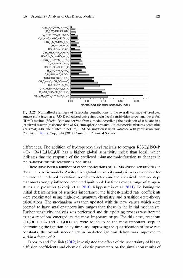
differences. The addition of hydroperoxyalkyl radicals to oxygen R33C4H9O2P

+O2¼R41C4H9O4UP has a higher global sensitivity index than local, which

indicates that the response of the predicted n-butane mole fraction to changes in

the A-factor for this reaction is nonlinear.

There have been a number of other applications of HDMR-based sensitivities in

chemical kinetic models. An iterative global sensitivity analysis was carried out for

the case of methanol oxidation in order to determine the chemical reaction steps

that most strongly influence predicted ignition delay times over a range of temper-

atures and pressures (Skodje et al. 2010; Klippenstein et al. 2011). Following the

initial determination of reaction importance, the highest-ranked rate coefficients

were reestimated using high-level quantum chemistry and transition-state-theory

calculations. The mechanism was then updated with the new values which were

deemed to have smaller uncertainty ranges than those in the initial mechanism.

Further sensitivity analysis was performed and the updating process was iterated

as new reactions emerged as the most important steps. For this case, reactions

CH3OH+HO2 and CH3OH+O2 were found to be the most important steps in

determining the ignition delay time. By improving the quantification of these rate

constants, the overall uncertainty in predicted ignition delays was improved to

within a factor of 2.

Esposito and Chelliah (2012) investigated the effect of the uncertainty of binary

diffusion coefficients and chemical kinetic parameters on the simulation results of

Fig. 5.25 Normalised estimates of first-order contributions to the overall variance of predicted

butane mole fraction at 750 K calculated using first-order local sensitivities (grey) and the global

HDMR method (black). Both are derived from a model describing the oxidation of n-butane in a

jet stirred reactor (residence time of 6 s, atmospheric pressure, stoichiometric mixtures containing

4 % (mol) n-butane diluted in helium). EXGAS notation is used. Adapted with permission from

Cord et al. (2012). Copyright (2012) American Chemical Society


premixed and non-premixed hydrogen–oxidiser–diluent flames. The most influen-

tial parameters were selected using the Morris method, and it was followed by

global sensitivity analysis based on the HDMR approach. The results indicated that

measured flame data can be used for a more accurate determination of the rate

parameters, but there is no possibility of reducing the diffusion coefficient uncer-

tainties in this way.

A global uncertainty analysis based on HDMR was also applied to the Regional

Atmospheric Chemical Mechanism (RACM) within a zero-dimensional photo-

chemical model in order to determine the main sources of uncertainty in predictions

of atmospheric OH and HO2 radicals (Chen et al. 2012). One aim was to highlight

parameters driving predictive uncertainty during periods when discrepancies

between modelled and measured OH and HO2 were greatest. The global sensitivity

analysis showed that modelled OH and HO2 depend most critically on the reactions

of xylenes and isoprene with OH, NO2 with OH, NO with HO2 and internal alkenes

with O3 and, in common with many combustion studies, therefore highlight the

need for better quantification of critical reaction rates. A similar approach was

applied to a model of urban ozone production in Chen and Brune (2012).

Uncertainty analyses based on polynomial chaos expansions have also been

applied to several kinetic systems. In Sheen and Wang (2011b) this approach was

applied to a detailed H2/CO/C1–C4 kinetic model using a set of experimental data

for ethylene combustion with the aim of providing further constraints on the model

input parameters. Uncertainty factors for each rate coefficient were propagated

through models for flame speed, flow reactor and ignition delay predictions. The

uncertainty propagation was also coupled with optimisation of the input rate

parameter coefficients based on a wide range of target experiments and their

uncertainties.

An example of the propagated uncertainties for the non-optimised (prior) model,

represented by 2σ bands, is shown in the left panel of Fig. 5.26 for predicted laminar

flame speeds, with the shaded regions showing the predicted pdf. The scatter in the

Fig. 5.26 Variation of laminar flame speed with equivalence ratio for ethylene–air flames,

P¼ 5 atm. Left panel: prior model. Right panel: posterior model. The shaded bands indicate the

2σ standard deviation on the model prediction uncertainty; shading intensity indicates the prob-

ability density, and the actual 2σ limits are indicated by the dashed lines. Reprinted from (Sheen

and Wang 2011a, b) with permission from Elsevier


predictive uncertainties are seen to be large in comparison to the scatter in experi-

mental measurements as was also suggested for the methane flame example in the

previous section. It demonstrates the need for further methods to reduce uncer-

tainties in predictive models, either by better quantification of rate coefficients

through fundamental kinetic experiments or theoretical calculations, or alterna-

tively through model optimisation. The right-hand panel of Fig. 5.26 shows the 2σbands when experimental measurements are used to further constrain the feasible

region of the sensitive input parameters. The 2σ bands are narrower in this case

indicating that incorporating constraints imposed by indirect experimental mea-

surements led to reductions in the overall uncertainty of the optimised model.

An interesting point to highlight here is that such predictive error bands will be

extremely sensitive to the selected input uncertainty factors f chosen for the study.

For large and complex kinetic mechanisms containing large numbers of estimated

parameters, or parameters derived from theoretical methods, obtaining accurate

values for f could be difficult. Since theoretical methods are becoming increasingly

used to estimate chemical kinetic parameters (Miller et al. 2005; Pilling 2009),

particularly in the gas phase, it is important to develop an understanding of the

uncertainties inherent in such approaches. A number of recent studies have there-

fore begun to assess the uncertainty in rate constants derived from theory calcu-

lations. An early example is from Goldsmith et al. (2013) who investigated the

potential uncertainties in deriving rate coefficients using transition-state-theory for

an example system of n-propyl +O2 based on input uncertainties in barrier heights,

well depths, vibrational frequencies, collision frequency and energy transfer para-

meters. The study showed that even when energies relative to n-propyl +O2 are

known to be within 1 kcal/mol, 3σ values in the predicted rate constants could be as

large as a factor of 10 for such a complex system with multiple transition states.

Similar findings were reported in Prager et al. (2013).

5.6.6 Handling Correlated Inputs Within Global Uncertaintyand Sensitivity Studies

As discussed in Sect. 5.6.2, a full evaluation of the input uncertainties to a model

should, where relevant, provide information on the correlations between input

parameters. This can be represented through the joint probability distribution of the

parameters or through a covariance matrix Σp such as that shown in Eq. (5.68). The

joint probability distribution of model parameters can be determined from experi-

mental data using the Bayes method (Berger 1985). Kraft et al. (Smallbone

et al. 2010; Mosbach et al. 2014), Braman et al. (2013) and Miki et al. (Panesi

et al. 2012; Miki et al. 2013) have calculated the pdf of rate parameters from

experimental data. The covariance matrix of the rate parameters was calculated

from the back propagation of experimental errors to the uncertainty of parameters

by Sheen et al. (Sheen et al. 2009, 2013; Sheen and Wang 2011a, b) and by [Turanyi


et al. (2012), Zsely et al. (2012), Varga et al. (2014, 2015)]. Confidence limits on

model predictions can then be obtained by propagating uncertainties in these corre-

lated inputs on predicted target outputs using, for example, a randomMonte Carlo or

quasi-random sampling procedure. As discussed in Sect. 5.5.2, a structured sampling

approach such as that obtained from a Sobol’ sequence might be preferred due to its

advantageous space filling and convergence properties. A joint probability distri-

bution, accounting for correlations expressed within the covariance matrix, can be

obtained from a starting Sobol’ sequence using a method described in Kucherenko

et al. (2012). The Sobol’ sequence is first transformed into a standard normal vectorexwith zero mean and unit variance using the inverse normal cumulative distribution

function. A Cholesky decomposition of the correlation matrix Σp is then performed:

Σp ¼ AAT ð5:89Þ

and a joint probability distribution of the parameters x is obtained fromex as follows:x ¼ Aex þ μ ð5:90Þ

Here μ is a matrix of the mean values for each parameter. As discussed in

Sect. 5.6.2, accounting for correlations between parameters is important if signif-

icant off-diagonal terms are present in the covariance matrix, since, otherwise, an

overestimation of the width of the predicted output distributions can occur.

Marginal sensitivities can then be determined for this correlated input–output

sample using the HDMR method described above, but in this case, because corre-

lations are present, the ordering of parameters within the transformations described

in Eqs. (5.89) and (5.90) affects the marginal sensitivities. A full variance decompo-

sition for correlated inputs requires all permutations of the Cholesky decomposition

to be used for the input sample generation, which adds to the computational cost of

the method. Methods for handling global sensitivity analysis based on correlated

inputs are described in Li et al. (2010), Li and Rabitz (2012), Mara and Tarantola

(2012), Kucherenko et al. (2012) and Zuniga et al. (2013). A general methodology

based on polynomial chaos expansions (see Sect. 5.5.5.2) is also outlined in Prager

et al. (2013) with application to a hydrocarbon ignition model. In particular this

study highlights the role of correlations within the Arrhenius parameters on

predicted ignition time for fuel–air mixtures.

5.7 Uncertainty Analysis in Systems Biology

We have already discussed the fact that significant uncertainties can exist in the

parameterisation of gas kinetic models and in theoretical calculations of rate

coefficients of relevance to gas-phase chemistry. In many applications within

gas-phase chemistry, however, the basic structure of the model is reasonably well

known or can be suggested using mechanism construction protocols such as those


discussed in Chap. 3. In some cases, the lack of agreement between modelled and

experimental data can force us to explore potentially missing reaction channels that

need to be added to mechanisms. In the majority of cases in systems biology, at

best, the qualitative structure of a model can be suggested, and time-series measure-

ments of the variables of interest (concentrations and fluxes) have been obtained

under certain conditions, but parameters remain very poorly quantified (Wilkinson

et al. 2008). This problem is commonly addressed by running a model with

estimated parameters and assessing how well the model agrees with the “target”

behaviour of the variables (based on, e.g., experimental measurements). The

parameters are then adjusted iteratively until a good fit to the target data is achieved.

This issue of parameter tuning was also referred to with respect to flame models in

Sect. 5.6.4. In the same way as for gas kinetic models, the system may well be

underdetermined, meaning that many combinations of parameters could in fact be

used to fit the same observed behaviour (Wilkinson et al. 2008). In worse situations,

the basic model structure may even be uncertain. Hence, applications of uncertainty

and sensitivity analysis should address potential structural as well as parametric

uncertainties within biological models. For example, Blanchard et al. (2011) carried

out a global sensitivity analysis of several models designed to interpret BOLD

(blood–oxygen-level dependent) signals aimed at improving the understanding of

links between neuronal activity and flow, and metabolic changes within models of

potential use for the interpretation of functional MRI data. A global sensitivity

study was carried out for three different models, and the work highlighted that

parameter importance was strongly dependent upon the way the flow�metabolism

relationship was implemented within the models (e.g. serial vs. parallel). Model

structure was therefore critical in accounting for the representation of the relation-

ship between oxygen supply by the flow vs. oxygen demand from neurons. Sensi-

tivity analysis therefore allows checks on whether the model formulations make

sense from a biological point of view.

Ay and Arnosti (2011) provide a similar discussion with respect to analytical

models of gene expression, where several major classes of model exist based on

thermodynamic, Boolean or differential equation approaches. The models

discussed in their review are suggested to contain large numbers of estimated

parameters and again uncertain model structures. A more detailed application of

global sensitivity analysis to a thermodynamic model of gene expression was

applied in Dresch et al. (2010) and highlighted that both biological effects and

mathematical model structures, could contribute to the observed importance rank-

ing of the parameters. In one case, parameters that were thought to describe the

system’s dependence on activator� activator cooperativity were found to exhibit

low sensitivities to the target output. However, even in such cases, sensitivity

analysis can provide useful information such as highlighting that the biological

relevance of certain aspects of a model may be weak. Thus, Ay and Arnosti (2011)

highlight the need for sensitivity analysis in assisting modellers to select appropri-

ate model formulations that best fit the biological system under investigation, as

well as highlighting which experiments will be most informative for improving

model parameterisations. For example, it would not make sense to design an

5.7 Uncertainty Analysis in Systems Biology 125

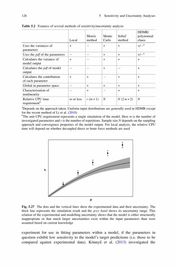
http://dx.doi.org/10.1007/978-3-662-44562-4_3

experiment for use in fitting parameters within a model, if the parameters in

question exhibit low sensitivity to the model’s target predictions (i.e. those to be

compared against experimental data). Konnyu et al. (2013) investigated the

Table 5.2 Features of several methods of sensitivity/uncertainty analysis

Local

Morris

method

Monte

Carlo

Sobol’

method

HDMR/

polynomial

chaos

Uses the variances of

parameters

+ � + + +/�a

Uses the pdf of the parameters � � + + +/�a

Calculates the variance of

model output

+ � + + +

Calculates the pdf of model

output

� � + � +

Calculates the contribution

of each parameter

+ + � + +

Global in parameter space � + + + +

Characterisation of

nonlinearity

� + � + +

Relative CPU time

requirementbm or less r (m + 1) N N (2m+ 2) N

aDepends on the approach taken. Uniform input distributions are generally used in HDMR except

for the recent method of Li et al. (2010)bThe unit CPU requirement represents a single simulation of the model. Here m is the number of

investigated parameters and r is the number of repetitions. Sample size N depends on the sampling

approach and convergence properties of the model output. For local analysis, the relative CPU

time will depend on whether decoupled direct or brute force methods are used

Fig. 5.27 The dots and the vertical lines show the experimental data and their uncertainty. The

thick line represents the simulation result and the grey band shows its uncertainty range. This

relation of the experimental and modelling uncertainty shows that the model is either structurally

inappropriate or that much larger uncertainties exist within the input parameters than were

assumed based on current knowledge


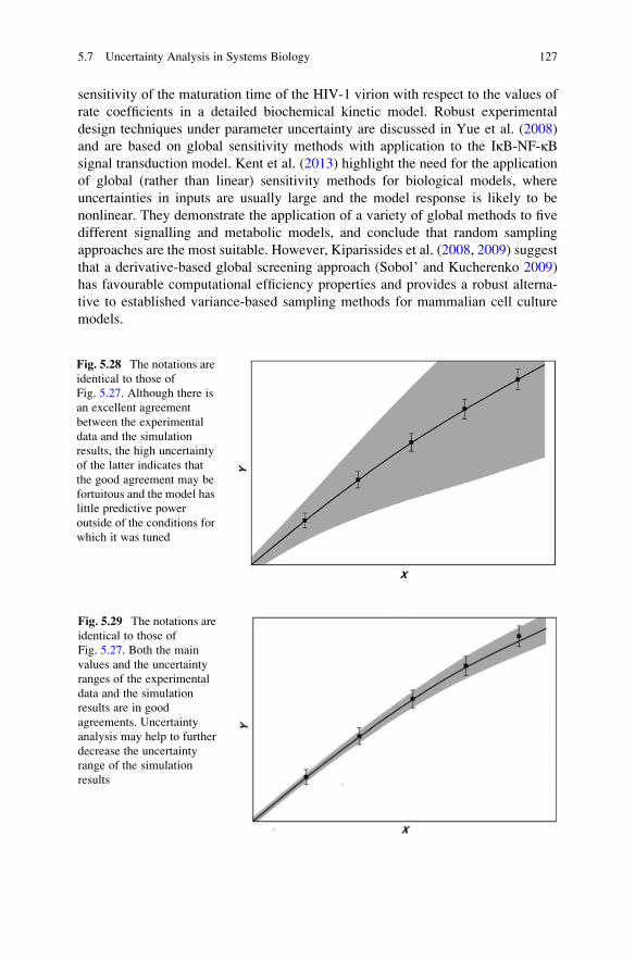
sensitivity of the maturation time of the HIV-1 virion with respect to the values of

rate coefficients in a detailed biochemical kinetic model. Robust experimental

design techniques under parameter uncertainty are discussed in Yue et al. (2008)

and are based on global sensitivity methods with application to the IκB-NF-κBsignal transduction model. Kent et al. (2013) highlight the need for the application

of global (rather than linear) sensitivity methods for biological models, where

uncertainties in inputs are usually large and the model response is likely to be

nonlinear. They demonstrate the application of a variety of global methods to five

different signalling and metabolic models, and conclude that random sampling

approaches are the most suitable. However, Kiparissides et al. (2008, 2009) suggest

that a derivative-based global screening approach (Sobol’ and Kucherenko 2009)

has favourable computational efficiency properties and provides a robust alterna-

tive to established variance-based sampling methods for mammalian cell culture

models.

Fig. 5.28 The notations are

identical to those of

Fig. 5.27. Although there is

an excellent agreement

between the experimental

data and the simulation

results, the high uncertainty

of the latter indicates that

the good agreement may be

fortuitous and the model has

little predictive power

outside of the conditions for

which it was tuned

Fig. 5.29 The notations are

identical to those of

Fig. 5.27. Both the main

values and the uncertainty

ranges of the experimental

data and the simulation

results are in good

agreements. Uncertainty

analysis may help to further

decrease the uncertainty

range of the simulation

results


Uncertainty Analysis: General Conclusions

In this chapter various methods applicable for sensitivity and uncertainty

analyses were reviewed, and the usual definitions of uncertainty information,

as given in chemical kinetic databases, were summarised. The uncertainty of

chemical kinetic models, calculated from the uncertainty of parameters, was

presented, for examples of simulations of a methane flame model. In this

section the general features of the various uncertainty analysis methods are

reviewed and some general conclusions are made.

Ideally, an uncertainty analysis method has the following features:

• It is global (i.e. the whole parameter space is explored).

• It is able to calculate the joint pdf of the simulation results from the joint

pdf of the model parameters.

• It calculates the contribution of the uncertainty of each parameter to the

overall uncertainty of the model results and thus provides a global sensi-

tivity measure.

• It is applicable even for large models with many input parameters.

• It has low computational requirements.

Not surprisingly, such an ideal method that is applicable to all model types

does not exist, since the requirements of the various features described above

have trade-offs against each other. In reality, the comprehensive analysis of a

model may require the combined application of several methods (Tebes-

Stevens and Valocchi 2000; Ratto and Paladino 2000). In particular, common

practice is to use computationally cheaper methods to screen out unimportant

parameters and then subsequently to perform a global analysis on a subset of

important input parameters. The features of various available methods are

summarised in Table 5.2.

Typically, local uncertainty analysis is based on the application of local

sensitivity coefficients, i.e. the partial derivatives of the model result with

respect to the parameters. Over the last few decades, very effective algo-

rithms were developed for the calculation of local sensitivity coefficients and

these can be obtained using low computational resources. The disadvantage

of local methods is that they are based on a linear approximation of the effect

of parameters, and therefore they are not applicable for highly nonlinear

models when the range of uncertainty of the parameters is wide, or if the

solution of the model is qualitatively different in different regions of the

domain of parameter uncertainty. Where the local coefficient is not available

as part of a single model simulation using the decoupled direct method, the

brute force approach may be taken, increasing the computational cost to order

m, where m is the number of parameters. For screening, one possible

approach is to use the calculation of local sensitivity coefficients at several

sets of nominal values for the parameters in order to identify those which

(continued)


have a low local sensitivity coefficient across the input range

(i.e. unimportant parameters). Local sensitivity coefficients are widely used

for the identification of parameters that can be estimated from a given set of

experimental data (Hessler and Ogren 1992; Ogren and Hessler 1995;

Turanyi et al. 2012). Nonlinear responses and parameter interactions could

then be explored using global methods for a subset of important parameters.

According to an ordering based on increasing CPU time requirements, the

next variety of methods should be the screening methods. These are global

methods, since several parameters are changed across a wide range. Such

methods, like the Morris method, provide approximate, qualitative informa-

tion about the uncertainty of the simulation results and the importance of the

parameters, and do include the effect of parameter interactions, although

these are not decomposed explicitly. For large parameter systems, however,

even the Morris method can become computationally costly since the method

is of the order r(m + 1), where r is the number of repeated parameter set series

required for the output mean and variance to converge. Each repeated para-

meter set series requires m + 1 model simulations. Nonlinear models with

strong interactions may require the number of Morris runs r to be quite large

in order to achieve convergence (Hughes et al. 2006).

The point of Monte Carlo methods is that all parameters of the model are

changed simultaneously according to their joint probability density functions

(pdfs) resulting in a histogram of the simulation results, which can be used for

the approximation of the pdf of the results. Monte Carlo methods usually have

large computational requirements, which can be decreased by Latin hyper-

cube sampling for smaller parameter systems or quasi-random sampling for

larger systems (see Sect. 5.5.2). The choice between using a stratified sam-

pling approach such as Latin hypercube or quasi-random approaches is not

easy to make a priori, since for random approaches, the sample size often

depends on the number of important parameters and the extent of parameter

interactions. However, Ziehn (2008) and Feil et al. (2009) have shown that for

a range of chemical models, quasi-random sampling approaches provide

faster convergence of the output statistics compared to Latin hypercube or

random Monte Carlo sampling. The advantage of Monte Carlo methods is

that they do not require special codes, and their application is conceptually

and practically quite easy. They are also able to use probabilistic samples

based on the input pdfs. However, Monte Carlo methods do not automatically

reveal the relative contribution of the parameters to the overall uncertainty of

the model output. This can be estimated via the calculation of Pearson or

Spearman correlation coefficients, but these have the limitation of expressing

only linear or monotonic relationships, respectively (Tomlin 2006).

The FAST method and the computation of the Sobol’ sensitivity indices do

not provide the joint pdf of the model results, but do give information about

(continued)


the variance of the results and the contributions of each parameter to these

variances. The common feature of these methods is that they use well-

designed pseudorandom numbers instead of real random numbers. Both

these methods have large CPU time requirements, however, and are therefore

mainly applicable for the study of models having few parameters or for the

analysis of the effect of a few parameters in a many-parameter model. The

few important parameters can be first identified using local uncertainty

analysis or a screening method.

Metamodel or response surface-based methods perhaps provide the best

balance between computational intensity and information about the partial

variances due to input parameter uncertainties. In many cases, the develop-

ment of an accurate metamodel can be achieved using a far smaller sample

size than that required by FAST or Sobol’s basic method. The metamodel is

then used for calculating global sensitivity indices. In common with the

Sobol’ method, HDMR, for example, is based on the analysis of variance.

Where higher-order terms (>2) in the HDMR expansion are weak, global

sensitivity indices can be achieved using a relatively small quasi-random

sample even for large parameter systems.

For the selection of an appropriate method, the available computational

and human resources, the number of parameters to be investigated, the

nonlinearity of the model and the intention of the study have to be taken

into account. If a single simulation of the model requires little CPU time

(e.g. not more than 1 minute) and the number of parameters investigated do

not exceed about 20, then the Sobol’ or FAST methods are applicable. If the

effect of 10 parameters is investigated and each run requires 0.5 min on a

desktop PC, then the calculation of the first-order and total indices requires

about 40–80 h on a single core. If the time needed for each simulation is

longer and the effect of more parameters is investigated, then the Morris

method would be appropriate. If the average and variance of the effects is

calculated on the basis of a 5-parameter set series, then the CPU time

requirement is also about 80 hours, although the accuracy would depend on

whether a 5-parameter set series was sufficient to gain convergence of the

output mean and variance. One disadvantage of the (original) Morris method

is that it does not take into account the pdf of the parameters during sampling.

Note that an enhanced version of the Morris method, called the radial designmethod, which takes into account the pdf is also available (Campolongo

et al. 2011; Saltelli et al. 2012). If each calculation requires more CPU

time and/or the effect of more parameters is investigated, but we would like to

calculate not only the variances of the model results but also the contributions

of the parameters to these variances, then local uncertainty analysis could be

applied. However, both of these are one-at-a-time approaches, which will fail

to explore parameter interactions, and the difference between local and global

(continued)


sensitivity indices could be large (Ziehn et al. 2009b; Saltelli and Annoni

2010). Local or one-at-a-time methods might be better used as prior screening

methods before the application of global sensitivity methods (Saltelli and

Annoni 2010). In fact, some of the more computationally efficient global

methods such as the extended version of HDMR developed by Ziehn

et al. can also be used without prior screening since unimportant component

functions are automatically excluded from the HDMR expansion based on the

use of an error threshold (Ziehn and Tomlin 2009). This allows the methods

to be applied to quite large kinetic mechanisms. For example, 176 input

parameters for a one-dimensional flame model were considered in Ziehn

and Tomlin (2008b) using a quasi-random sample of only 1,024 runs.

Metamodel and Monte Carlo methods are applicable for the unbiased

estimation of the variance of the model results, even for multiparameter

models. This is especially important when we want to investigate if the ranges

of uncertainty of the simulation results overlap with those of the experimental

data or whether there is a systematic deviation between these quantities.

For example, if we use a random sample which covers the whole possible

input space and none of the simulations overlap within experimental error for

a given target experiment, then this suggests that there are missing model

components or inappropriate parameterisations within the model. Missing

reaction channels or perhaps missing physical processes such as inappropriate

descriptions of mixing, or reactor wall or boundary processes may be the

reason. The identification of important input parameters and possibly in-

appropriate model structure both form a very useful part of the model

evaluation processes. Or at least they should do!

Several authors have criticised variance-based methods for global sensi-

tivity analysis however, and moment-independent methods are now starting

to emerge which take account of changes to the whole output pdf uponchanges in input parameters, rather than simply measures such as variance,

as briefly discussed in Sect. 5.5.6. Whilst only limited applications of such

methods have been seen for kinetic models so far, this could be an interesting

area for future research.

The basic methods of global uncertainty/sensitivity analysis have been

elaborated over several decades, and computer codes have been made avail-

able by several research groups (see Chap. 9). It is therefore surprising that

uncertainty analyses of relatively few reaction kinetic models have been

carried out so far. Possible barriers are the large computational requirements

as well as the need for accurate knowledge of uncertainties in the input

parameters. The former means that a global uncertainty analysis requires

simulation of the full model using several thousand different parameter

sets. Due to the increasing speed and capacity of computers, this is becoming

less of a problem. Knowledge about chemical kinetics is also rapidly

(continued)


http://dx.doi.org/10.1007/978-3-662-44562-4_9

increasing, which means that the values of more and more parameters are

being determined by fundamental methods rather than through estimation.

For well-known systems, some parameters have been measured several times,

which provides additional information about the uncertainty of these param-

eters. As a consequence, it is expected that more and more studies will be

published where the aim is not to simply demonstrate the abilities of an

uncertainty analysis for a chemical kinetics example, but rather to acquire

chemical knowledge using well-based uncertainty analysis. An example of

model improvement based on global uncertainty analysis for the case of

methanol oxidation using this approach is demonstrated in Skodje

et al. (2010).

Following the review of available methods for uncertainty/sensitivity

analysis, let us summarise why these methods are important for the investi-

gation of numerical models.

1. Uncertainty analysis may help to decide if our model is structurally

appropriate (Furbringer and Roulet 1999; Tomlin and Ziehn 2011) as

discussed above. Identifying whether the performance and reliability of

the model could be best improved by improving the quantification of key

parameters or require changes to the model structure should be a key part

of model evaluation (see Fig. 5.27).

2. Uncertainty analysis may also help to highlight whether or not our model

is robust. If changing the model parameters within their uncertainty limits

significantly changes the results of the model, then it is difficult to argue

that the model can be used as a predictive one (see Fig. 5.28). A model is

called predictive if it not only reproduces the previous experimental data

but provides reliable simulations at other more-or-less similar conditions.

Some models may well describe limited target experimental data, but

changing the parameters within their uncertainty limits may lead to

entirely different results. Trusting the extrapolation of the model to new

conditions therefore becomes problematic leaving the model of limited

applicability within, e.g., engineering design processes or strategic plan-

ning for air quality in atmospheric models. However, uncertainty analysis

is able to help to identify such shortcomings of a model and to provide

confidence limits on its predictions, not just for conditions where experi-

ments have been performed, but across very wide sets of conditions. In

fields such as environmental and social sciences, and economics, it is

especially dangerous to make regulatory or financial decisions on the

basis of models that are not robust (Jakeman et al. 2006; van Delden

et al. 2011; Saltelli and Funtowicz 2014). Sensitivity and uncertainty

analyses should therefore be an important part of the development of

models which are used in design and decision-making processes.

(continued)


3. Next let us assume that the model is relatively robust, i.e. the ranges of

uncertainty of the experimental data and the corresponding model results

overlap and the range of uncertainty of the simulation results is not too

wide (see Fig. 5.29). Even such a model can be improved by further using

sensitivity analysis, because the parameters that cause most of the uncer-

tainty of the model outputs can be identified. In addition, experience shows

that even if the original model contained several hundred or even several

thousands of parameters, most of the uncertainty of the model results is

caused by only a few of them. This means that if these parameters were

better known (i.e. with less uncertainty), then the uncertainty of the simula-

tion results could be significantly decreased. Efforts can then be concentrated

on the better characterisation of these parameters (Skodje et al. 2010).

4. Sensitivity analysis may also assist in experimental design. If several key

parameters have been identified as driving the model uncertainty, then new

experimental studies may be required in order to provide their better

quantification (Sheen and Manion, 2014). A useful experiment is one

that provides additional constraints on the parameter of interest, and

therefore, a large sensitivity of predicted experimental targets to changes

in that parameter is required.

References

Androulakis, I.P.: “Store and retrieve” representations of dynamic systems motivated by studies in

gas phase chemical kinetics. Comput. Chem. Eng. 28, 2141–2155 (2004)

Atherton, R.W., Schainker, R.B., Ducot, E.R.: On the statistical sensitivity analysis of models for

chemical kinetics. AIChE J. 21, 441–448 (1975)



Volume I—gas phase reactions of Ox, HOx, NOx and SOx species. Atmos. Chem. Phys. 4,

1461–1738 (2004)


Rossi, M.J., Troe, J.: IUPAC_Subcommittee: evaluated kinetic and photochemical data for

atmospheric chemistry: Volume II—gas phase reactions of organic species. Atmos. Chem.

Phys. 6, 3625–4055 (2006)



Volume III—gas phase reactions of inorganic halogens. Atmos. Chem. Phys. 7, 981–1191

(2007)


Rossi, M.J., Troe, J., Wallington, T.J.: Evaluated kinetic and photochemical data for atmo-

spheric chemistry: Volume IV—gas phase reactions of organic halogen species. Atmos. Chem.

Phys. 8, 4141–4496 (2008)

Ay, A., Arnosti, D.N.: Mathematical modeling of gene expression: a guide for the perplexed

biologist. Crit. Rev. Biochem. Mol. Biol. 46, 137–151 (2011)

Balakrishnan, S., Georgopoulos, P., Banerjee, I., Ierapetritou, M.: Uncertainty consideration for

describing complex reaction systems. AIChE J. 48, 2875–2889 (2002)

References 133

Battin-Leclerc, F.: Detailed chemical kinetic models for the low-temperature combustion of

hydrocarbons with application to gasoline and diesel fuel surrogates. Prog. Energy Combust.

Sci. 34, 440–498 (2008)

Baulch, D.L., Cobos, C.J., Cox, R.A., Esser, C., Frank, P., Just, T., Kerr, J.A., Pilling, M.J., Troe,

J., Walker, R.W., Warnatz, J.: Evaluated kinetic data for combustion modeling. J. Phys. Chem.

Ref. Data 21, 411–734 (1992)

Baulch, D.L., Cobos, C.J., Cox, R.A., Frank, J.H., Hayman, G., Just, T.H., Kerr, J.A., Murrels, T.,

Pilling, M.J., Troe, J., Walker, B.F., Warnatz, J.: Summary table of evaluated kinetic data for

combustion modeling—Supplement-1. Combust. Flame 98, 59–79 (1994)




Berger, J.O.: Statistical Decision Theory and Bayesian Analysis. Springer, New York (1985)

Bischof, C., Carle, A., Khademi, P.: Mauer: the ADIFOR 2.0 system for the automatic differen-

tiation of FORTRAN 77 programes. IEEE J. Comput. Sci. Eng. 3, 18–32 (1996)

Bischof, C.H., Roh, L., Mauer-Oats, A.J.: ADIC: an extensible automatic differentiation tool for

ANSI-C. Softw. Pract. Exp. 27, 1427–1456 (1997)

Bischof, C.H., Bucker, H.M., Rasch, A.: Sensitivity analysis of turbulence models using automatic

differentiation. SIAM J. Sci. Comput. 26, 510–522 (2004)

Blanchard, S., Papadopoulo, T., Benar, C.G., Voges, N., Clerc, M., Benali, H., Warnking, J.,

David, O., Wendling, F.: Relationship between flow and metabolism in BOLD signals: insights

from biophysical models. Brain Topogr. 24, 40–53 (2011)

Blatman, G., Sudret, B.: Efficient computation of global sensitivity indices using sparse polyno-

mial chaos expansions. Reliab. Eng. Syst. Saf. 95, 1216–1229 (2010)

Borgonovo, E., Tarantola, S.: Moment independent and variance-based sensitivity analysis with

correlations: an application to the stability of a chemical reactor. Int. J. Chem. Kinet. 40, 687–

698 (2008)

Borgonovo, E., Castaings, W., Tarantola, S.: Moment independent importance measures: new

results and analytical test cases. Risk Anal. 31, 404–428 (2011)

Bosschaart, K.J., de Goey, L.P.H.: Detailed analysis of the heat flux method for measuring burning

velocities. Combust. Flame 132, 170–180 (2003)

Braman, K., Oliver, T.A., Raman, V.: Bayesian analysis of syngas chemistry models. Combust.

Theory Model. 17, 858–887 (2013)

Brown, N.J., Revzan, K.L.: Comparative sensitivity analysis of transport properties and reaction

rate coefficients. Int. J. Chem. Kinet. 37, 538–553 (2005)

Brown, M.J., Smith, D.B., Taylor, S.C.: Influence of uncertainties in rate constants on computed

burning velocities. Combust. Flame 117, 652–656 (1999)

Campolongo, F., Tarantola, S., Saltelli, A.: Tackling quantitatively large dimensionality problems.

Comp. Phys. Commun. 117, 75–85 (1999)

Campolongo, F., Cariboni, J., Saltelli, A., Schoutens, W.: Enhancing the Morris method.

Proceedings of 4th International Conference on Sensitivity Analysis of Model Output

(SAMO 2004), pp. 369–379 (2005)

Campolongo, F., Cariboni, J., Saltelli, A.: An effective screening design for sensitivity analysis of

large models. Environ. Model. Software 22, 1509–1518 (2007)

Campolongo, F., Cariboni, J., Saltelli, A., Schoutens, W.: Enhancing the Morris method. Pro-

ceedings of 4th International Conference on Sensitivity Analysis of Model Output (SAMO

2004), pp. 369–379 (2005)

Campolongo, F., Saltelli, A., Cariboni, J.: From screening to quantitative sensitivity analysis. A

unified approach. Comput. Phys. Commun. 182, 978–988 (2011)

Carrasco, N., Pernot, P.: Modeling of branching ratio uncertainty in chemical networks by

Dirichlet distributions. J. Phys. Chem. A 111, 3507–3512 (2007)


Carrasco, N., Dutuit, O., Thissen, R., Banaszkiewicz, M., Pernot, P.: Uncertainty analysis of

bimolecular reactions in Titan ionosphere chemistry model. Planetary Space Sci. 55, 141–157

(2007)

Carrasco, N., Alcaraz, C., Dutuit, O., Plessis, S., Thissen, R., Vuitton, V., Yelle, R., Pernot, P.:

Sensitivity of a Titan ionospheric model to the ion-molecule reaction parameters. Planetary

Space Sci. 56, 1644–1657 (2008a)

Carrasco, N., Plessis, S., Dobrijevic, M., Pernot, P.: Toward a reduction of the bimolecular

reaction model for Titan’s ionosphere. Int. J. Chem. Kinet. 40, 699–709 (2008b)

Carslaw, N., Jacobs, P.J., Pilling, M.J.: Modeling OH, HO2, and RO2 radicals in the marine

boundary layer 2. Mechanism reduction and uncertainty analysis. J. Geophys. Res. D 104,

30257–30273 (1999)

Charzynska, A., Nałecz, A., Rybinski, M., Gambin, A.: Sensitivity analysis of mathematical

models of signaling pathways. BioTechnologia 93, 291–308 (2012)

Chen, S., Brune, W.H.: Global sensitivity analysis of ozone production and O3-NOx-VOC

limitation based on field data. Atmos. Environ. 55, 288–296 (2012)

Chen, S., Brune, W.H., Oluwole, O.O., Kolb, C.E., Bacon, F., Li, G.Y., Rabitz, H.: Global

sensitivity analysis of the regional atmospheric chemical mechanism: an application of random

sampling-high dimensional model representation to urban oxidation chemistry. Environ. Sci.

Technol. 46, 11162–11170 (2012)

Cheng, H.Y., Sandu, A.: Uncertainty quantification and apportionment in air quality models using

the polynomial chaos method. Environ. Model. Software 24, 917–925 (2009)

Clarke, A.G., Tomlin, A.S.: The atmosphere. In: Harrison, R.M. (ed.) Understanding Our Envi-

ronment. Royal Society of Chemistry, Cambridge (1999)

Considine, D.B., Stolarski, R.S., Hollandsworth, S.M., Jackman, C.H., Fleming, E.L.: A Monte

Carlo uncertainty analysis of ozone trend predictions in a two-dimensional model. J. Geophys.

Res. Atm. 104, 1749–1765 (1999)

Cord, M., Sirjean, B., Fournet, R., Tomlin, A., Ruiz-Lopez, M., Battin-Leclerc, F.: Improvement

of the modeling of the low-temperature oxidation of n-butane: study of the primary reactions.

J. Phys. Chem. A 116, 6142–6158 (2012)

Csaszar, A.G., Furtenbacher, T.: From a network of computed reaction enthalpies to atom-based

thermochemistry (NEAT). Chem. Eur. J. 16, 4826–4835 (2010)

Cukier, R., Fortuin, C., Shuler, K., Petschek, A., Schaibly, J.H.: Study of the sensitivity of coupled

reaction systems to uncertainties in rate coefficients I. Theory. J. Chem. Phys. 59, 3873–3878

(1973)

Cukier, R.I., Schaibly, J.H., Shuler, K.E.: Study of sensitivity of coupled reaction systems to

uncertainties in rate coefficients 3. Analysis of approximations. J. Chem. Phys. 63, 1140–1149

(1975)

Cukier, R.I., Levine, H.B., Shuler, K.E.: Nonlinear sensitivity analysis of multiparameter model

systems. J. Phys. Chem. 81, 2365–2366 (1977)

Cukier, R.I., Levine, H.B., Shuler, K.E.: Nonlinear sensitivity analysis of multi-parameter model

systems. J. Comput. Phys. 26, 1–42 (1978)

Daescu, D., Sandu, A., Carmichael, G.R.: Direct and adjoint sensitivity analysis of chemical

kinetic systems with KPP: Part II—Validation and numerical experiments. Atmos. Environ.

37, 5097–5114 (2003)

Damian, V., Sandu, A., Damian, M., Potra, F., Carmichael, G.R.: The kinetic PreProcessor KPP—

a software environment for solving chemical kinetics. Comp. Chem. Eng. 26, 1567–1579

(2002)

Davis, M.J., Skodje, R.T., Tomlin, A.S.: Global sensitivity analysis of chemical-kinetic reaction

mechanisms: construction and deconstruction of the probability density function. J. Phys.

Chem. A 115, 1556–1578 (2011)

Degasperi, A., Gilmore, S.: Sensitivity analysis of stochastic models of bistable biochemical

reactions. Lect. Notes Comput. Sci. 5016, 1–20 (2008)

References 135

Derwent, R.G.: Treating uncertainty in models of the atmospheric chemistry of nitrogen com-

pounds. Atmos. Environ. 21, 1445–1454 (1987)

Derwent, R., Hov, Ø.: Application of sensitivity and uncertainty analysis techniques to a photo-

chemical ozone model. J. Geophys. Res. Atm. 93, 5185–5199 (1988)

Dickinson, R.P., Gelinas, R.J.: Sensitivity analysis of ordinary differential equation systems—

direct method. J. Comput. Phys. 21, 123–143 (1976)

Djouad, R., Audiffren, N., Sportisse, B.: A sensitivity analysis study for RADM2mechanism using

automatic differentiation. Atmos. Environ. 37, 3029–3038 (2003)

Dobrijevic, M., Carrasco, N., Hebrard, E., Pernot, P.: Epistemic bimodality and kinetic hypersen-

sitivity in photochemical models of Titan’s atmosphere. Planetary Space Sci. 56, 1630–1643

(2008)

Dobrijevic, M., Hebrard, E., Plessis, S., Carrasco, N., Pernot, P., Bruno-Claeys, M.: Comparison of

methods for the determination of key reactions in chemical systems: application to Titan’satmosphere. Adv. Space Res. 45, 77–91 (2010)

Dresch, J.M., Liu, X.Z., Arnosti, D.N., Ay, A.: Thermodynamic modeling of transcription:

sensitivity analysis differentiates biological mechanism from mathematical model-induced

effects. BMC Syst. Biol. 4, 142 (2010)

Dunker, A.M.: Efficient calculation of sensitivity coefficients for complex atmospheric models.

Atmos. Environ. 15, 1155–1161 (1981)

Dunker, A.M.: The decoupled direct method for calculating sensitivity coefficients in chemical

kinetics. J. Chem. Phys. 81, 2385–2393 (1984)

Edelson, D., Allara, D.L.: A computational analysis of the alkane pyrolysis mechanism: sensitivity

analysis of individual reaction steps. Int. J. Chem. Kinet. 12, 605–621 (1980)

Edelson, D., Thomas, V.M.: Sensitivity analysis of oscillating reactions. J. Phys. Chem. 85, 1555–

1558 (1981)

Esposito, G., Chelliah, H.K.: Effect of binary diffusion and chemical kinetic parameter uncer-

tainties in simulations of premixed and non-premixed laminar hydrogen flames. Combust.

Flame 159, 3522–3529 (2012)

Faure, H.: Good permutations for extreme discrepancy. J. Num. Theor. 42, 47–56 (1992)

Faure, C.: An automatic differentiation platform: Odyssee. Fut. Gen. Comput. Sys. 21, 1391–1400

(2005)

Feil, B., Kucherenko, S., Shah, N., IEEE: Comparison of Monte Carlo and Quasi Monte Carlo

sampling methods in high dimensional model representation. SIMUL: 2009 First International

Conference on Advances in System Simulation. IEEE, New York (2009)

Feng, X.-J., Hooshangi, S., Chen, D., Li, G., Weiss, R., Rabitz, H.: Optimizing genetic circuits by

global sensitivity analysis. Biophys. J. 87, 2195–2202 (2004)

Furbringer, J.-M., Roulet, C.-A.: Confidence of simulation results: put a sensitivity analysis

module in your MODEL. The IEA-ECBCS Annex 23 experience of model evaluation. Energy

Build 30, 61–71 (1999)

Galanti, S., Jung, A.: Low-discrepancy sequences: Monte Carlo simulation of option prices. J.

Deriv. 5, 63–83 (1997)

Gao, D., Stockwell, W.R., Milford, J.B.: First-order sensitivity and uncertainty analysis for a

regional-scale gas-phase chemical mechanism. J. Geophys. Res. Atm. 100, 23153–23166

(1995)

Gao, D.F., Stockwell, W.R., Milford, J.B.: Global uncertainty analysis of a regional-scale

gas-phase chemical mechanism. J. Geophys. Res. Atm. 101, 9107–9119 (1996)

Goldsmith, C.F., Tomlin, A.S., Klippenstein, S.J.: Uncertainty propagation in the derivation of

phenomenological rate coefficients from theory: a case study of n-propyl radical oxidation.Proc. Combust. Inst. 34, 177–185 (2013)

Gunawan, R., Cao, Y., Petzold, L., Doyle, F.J.: Sensitivity analysis of discrete stochastic systems.

Biophys. J. 88, 2530–2540 (2005)

Halton, J.H.: On the efficiency of certain quasi-random sequences of points in evaluating multi-

dimensional integrals. Numerische Mathematik 2, 84–90 (1960)


He, S., Carmichael, G.R., Sandu, A., Hotchkiss, B., Damian-Iordache, V.: Application of ADIFOR

for air pollution model sensitivity studies. Environ. Model. Software 15, 549–557 (2000)

Hebrard, E., Dobrijevic, M., Pernot, P., Carrasco, N., Bergeat, A., Hickson, K.M., Canosa, A., Le

Picard, S.D., Sims, I.R.: Howmeasurements of rate coefficients at low temperature increase the

predictivity of photochemical models of Titan’s atmosphere. J. Phys. Chem. A 113, 11227–

11237 (2009)

Helton, J.C., Davis, F.J.: Latin hypercube sampling and the propagation of uncertainty in analyses

of complex systems. Reliab. Eng. Syst. Saf. 81, 23–69 (2003)

Helton, J.C., Johnson, J.D., Sallaberry, C.J., Storlie, C.B.: Survey of sampling-based methods for

uncertainty and sensitivity analysis. Reliab. Eng. Syst. Saf. 91, 1175–1209 (2006)

Hessler, J.P., Ogren, P.J.: Correlation analysis of complex kinetic systems: a new scheme for

utilizing sensitivity coefficients. J. Chem. Phys. 97, 6249 (1992)

Homma, T., Saltelli, A.: Importance measures in global sensitivity analysis of nonlinear models.

Reliab. Eng. Syst. Saf. 52, 1–17 (1996)

Hovland, P.D., Norris, B., Mills Strout, M., Bhowmick, S., Utke, J.: Sensitivity analysis and design

optimization through automatic differentiation. J. Phys. Conf. Ser. 16, 466–470 (2005)

Hughes, K.J., Tomlin, A.S., Hampartsoumian, E., Nimmo, W., Zsely, I.G., Ujvari, M., Turanyi, T.,

Clague, A.R., Pilling, M.J.: An investigation of important gas-phase reactions of nitrogenous

species from the simulation of experimental measurements in combustion systems. Combust.

Flame 124, 573–589 (2001a)

Hughes, K.J., Turanyi, T., Clague, A.R., Pilling, M.J.: Development and testing of a comprehen-

sive chemical mechanism for the oxidation of methane. Int. J. Chem. Kinet. 33, 513–538

(2001b)

Hughes, K.J., Griffiths, J.F., Fairweather, M., Tomlin, A.S.: Evaluation of models for the low

temperature combustion of alkanes through interpretation of pressure-temperature ignition

diagrams. PCCP 8, 3197–3210 (2006)

Hwang, J.T.: Nonlinear sensitivity analysis in chemical kinetics. Proc. Natl. Sci. Council B. ROC

6, 20–29 (1982)

Hwang, J.T., Dougherty, E.P., Rabitz, S., Rabitz, H.: Greens function method of sensitivity

analysis in chemical kinetics. J. Chem. Phys. 69, 5180–5191 (1978)

Ihekwaba, A.E., Broomhead, D.S., Grimley, R.L., Benson, N., Kell, D.B.: Sensitivity analysis of

parameters controlling oscillatory signalling in the NF-κB pathway: the roles of IKK and IκBα.Syst. Biol. 1, 93–103 (2004)

Ingalls, B.P.: Autonomously oscillating biochemical systems: parametric sensitivities of extrema

and period. IEE Syst. Biol. 1, 62–70 (2004)

Isukapalli, S.S., Roy, A., Georgopoulos, P.G.: Efficient sensitivity/uncertainty analysis using the

combined stochastic response surface method and automated differentiation: application to

environmental and biological systems. Risk Anal. 20, 591–602 (2000)

IUPAC Task Group on Atmospheric Chemical Kinetic Data Evaluation (2014) http://iupac.pole-

ether.fr/

Jakeman, A.J., Letcher, R.A., Norton, J.P.: Ten iterative steps in development and evaluation of

environmental models. Environ. Model. Software 21, 602–614 (2006)

JCGM: International vocabulary of metrology—Basic and general concepts and associated terms

(VIM). http://www.bipm.org/ (2008)

Kee, R.J., Grcar, J.F., Smooke, M.D., Miller, J.A.: PREMIX: A FORTRAN program for modeling

steady laminar one-dimensional premixed flames. Sandia National Laboratories (1985)

Kent, E., Neumann, S., Kummer, U., Mendes, P.: What can we learn from global sensitivity

analysis of biochemical systems? PLoS One 8, e79244 (2013)Kiparissides, A., Rodriguez-Fernandez, M., Kucherenko, S., Mantalaris, A., Pistikopoulos, E.:

Application of global sensitivity analysis to biological models. In: Braunschweig, B., Joulia,

X. (eds.) 18th European Symposium on Computer Aided Process Engineering. Computer-

Aided Chemical Engineering, vol. 25, pp. 689–694. Elsevier Science Bv, Amsterdam (2008)

References 137

http://iupac.pole-ether.fr/

http://iupac.pole-ether.fr/

http://www.bipm.org/

Kiparissides, A., Kucherenko, S.S., Mantalaris, A., Pistikopoulos, E.N.: Global sensitivity analysis

challenges in biological systems modeling. Ind. Eng. Chem. Res. 48, 7168–7180 (2009)

Klippenstein, S.J., Harding, L.B., Davis, M.J., Tomlin, A.S., Skodje, R.T.: Uncertainty driven

theoretical kinetics studies for CH3OH ignition: HO2+CH3OH and O2+CH3OH. Proc. Com-

bust. Inst. 33, 351–357 (2011)

Konnov, A.A.: Remaining uncertainties in the kinetic mechanism of hydrogen combustion.

Combust. Flame 152, 507–528 (2008)

Konnyu, B., Sadiq, S.K., Turanyi, T., Hırmondo, R., Muller, B., Krausslich, H.G., Coveney, P.V.,

Muller, V.: Gag-Pol processing during HIV-1 virion maturation: a systems biology approach.

PLoS Comput. Biol. 9, e1003103 (2013)

KPP: Kinetic Preprocessor. http://people.cs.vt.edu/~asandu/Software/Kpp/

Kramer, M.A., Calo, J.M., Rabitz, H.: An improved computational method for sensitivity analy-

sis—Greens function method with AIM. Appl. Math. Model. 5, 432–441 (1981)

Kramer, M.A., Rabitz, H., Calo, J.M., Kee, R.J.: Sensitivity analysis in chemical kinetics—recent

developments and computational comparisons. Int. J. Chem. Kinet. 16, 559–578 (1984)

Kucherenko, S.: Application of global sensitivity indices for measuring the effectiveness of quasi-

Monte Carlo methods and parameter estimation. In: 5th International Conference on Sensitiv-

ity Analysis of Model Output, Budapest, pp. 35–36 (2007)

Kucherenko, S., Tarantola, S., Annoni, P.: Estimation of global sensitivity indices for models with

dependent variables. Comput. Phys. Commun. 183, 937–946 (2012)

Kumar, K., Sung, C.J.: Autoignition of methanol: experiments and computations. Int. J. Chem.

Kinet. 43, 175–184 (2011)

Larter, R.: Sensitivity analysis of autonomous oscillators. Separation of secular terms and deter-

mination of structural stability. J. Phys. Chem. 87, 3114–3121 (1983)

Leloup, J.-C., Goldbeter, A.: Modeling the mammmalian circadian clock: sensitivity analysis and

multiplicity of oscillatory mechanisms. J. Theor. Biol. 230, 541–562 (2004)

Li, G.Y., Rabitz, H.: General formulation of HDMR component functions with independent and

correlated variables. J. Math. Chem. 50, 99–130 (2012)

Li, G., Rosenthal, C., Rabitz, H.: High dimensional model representations. J. Phys. Chem. A 105,

7765–7777 (2001)

Li, G., Wang, S.-W., Rabitz, H.: Practical approaches to construct RS-HDMR component func-

tions. J. Phys. Chem. A 106, 8721–8733 (2002a)

Li, G., Wang, S.-W., Rabitz, H., Wang, S., Jaffe, P.: Global uncertainty assessments by high

dimensional model representations (HDMR). Chem. Eng. Sci. 57, 4445–4460 (2002b)

Li, G.Y., Rabitz, H., Yelvington, P.E., Oluwole, O.O., Bacon, F., Kolb, C.E., Schoendorf, J.:

Global sensitivity analysis for systems with independent and/or correlated inputs. J. Phys.

Chem. A 114, 6022–6032 (2010)

Lu, B., Yue, H.: Sensitivity analysis of oscillatory biological systems with a SVD-based algorithm.

Syst. Inform. World Netw. 10, 37–47 (2010)

Ludtke, N., Panzeri, S., Brown, M., Broomhead, D.S., Knowles, J., Montemurro, M.A., Kell, D.B.:

Information-theoretic sensitivity analysis: a general method for credit assignment in complex

networks. J. R. Soc. Interface. 26 (2007)

Mara, T.A., Tarantola, S.: Variance-based sensitivity indices for models with dependent inputs.

Reliab. Eng. Syst. Saf. 107, 115–121 (2012)

Marinov, N.M., Pitz, W.J., Westbrook, C.K., Castaldi, M.J., Senkan, S.M.: Modeling of aromatic

and polycyclic aromatic hydrocarbon formation in premixed methane and ethane flames.

Combust. Sci. Technol. 116, 211–287 (1996)

McKay, M.D., Beckman, R.J., Conover, W.J.: A comparison of three methods for selecting values

of input variables in the analysis of output from a computer code. Technometrics 42, 55–61

(2000)

Miki, K., Prudencio, E.E., Cheung, S.H., Terejanu, G.: Using Bayesian analysis to quantify

uncertainties in the H+O2!OH+O reaction. Combust. Flame 160, 861–869 (2013)


http://people.cs.vt.edu/~asandu/Software/Kpp/

Miller, J.A., Pilling, M.J., Troe, J.: Unravelling combustion mechanisms through a quantitative

understanding of elementary reactions. Proc. Combust. Inst. 30, 43–88 (2005)

Mittal, G., Sung, C.J., Fairweather, M., Tomlin, A.S., Griffiths, J.F., Hughes, K.J.: Significance of

the HO2+CO reaction during the combustion of CO+H2 mixtures at high pressures. Proc.

Combust. Inst. 31, 419–427 (2007)

Morokoff, W., Caflisch, R.: Quasi-Monte Carlo Integration. J. Comput. Phys. 122, 218–230 (1995)

Morris, M.D.: Factorial sampling plans for preliminary computational experiments.

Technometrics 33, 161–174 (1991)

Morris, M.D.: Input screening: finding the important model inputs on a budget. Reliab. Eng. Syst.

Saf. 91, 1252–1256 (2006)

Mosbach, S., Hong, J.H., Brownbridge, G.P.E., Kraft, M., Gudiyella, S., Brezinsky, K.: Bayesian

error propagation for a kinetic model of n-propylbenzene oxidation in a shock tube. Int.

J. Chem. Kinet. 46, 389–404 (2014)

Moulik, M.D., Milford, J.B.: Factors influencing ozone chemistry in subsonic aircraft plumes.

Atmos. Environ. 33, 869–880 (1999)

Nagy, T., Turanyi, T.: Uncertainty of Arrhenius parameters. Int. J. Chem. Kinet. 43, 359–378

(2011)

Nagy, T., Turanyi, T.: Determination of the uncertainty domain of the Arrhenius parameters

needed for the investigation of combustion kinetic models. Reliab. Eng. Syst. Saf. 107, 29–

34 (2012)

Najm, H.N., Malorani, M.: Enforcing positivity in intrusive PC-UQ methods for reactive ODE

systems. J. Comp. Phys. 270, 544–569 (2014)

Najm, H., Debusschere, B.J., Marzouk, Y.M., Widmer, S., Le Maıtre, O.P.: Uncertainty quanti-

fication in chemical systems. Int. J. Numer. Meth. Eng. 80, 789–814 (2009)

Niederreiter, H.: Low-discrepancy and low-dispersion sequences. J. Num. Theor. 30, 51–70

(1988)

Nikolaev, E.V., Atlas, J.C., Shuler, M.L.: Sensitivity and control analysis of periodically forced

reaction networks using the Green’s function method. J. Theor. Biol. 247, 442–461 (2007)

Oakley, J., O’Hagan, A.: Bayesian inference for the uncertainty distribution of computer model

outputs. Biometrika 89, 769–784 (2002)

Oakley, J.E., O’Hagan, A.: Probabilistic sensitivity analysis of complex models: a Bayesian

approach. J. R. Stat. Soc. Ser. B (Stat. Methodol.) 66, 751–769 (2004)

Ogren, P.J., Hessler, J.P.: Sensitivity and correlation analysis of the physical parameters in

absorption, four-wave mixing, and Schlieren experiments. Int. J. Chem. Kinet. 27, 719–738

(1995)

Panesi, M., Miki, K., Prudhomme, S., Brandis, A.: On the assessment of a Bayesian validation

methodology for data reduction models relevant to shock tube experiments. Comput. Methods

Appl. Mech. Eng. 213–216, 383–398 (2012)

Pantazis, Y., Katsoulakis, M.A., Vlachos, D.G.: Parametric sensitivity analysis for biochemical

reaction networks based on pathwise information theory. BMC Bioinform. 14, 311 (2013)

Peng, Z., Dobrijevic, M., Hebrard, E., Carrasco, N., Pernot, P.: Photochemical modeling of Titan

atmosphere at the “10 percent uncertainty horizon”. Faraday Discuss. 147, 137–153 (2010)

Perger, T., Kovacs, T., Turanyi, T., Trevino, C.: Determination of adsorption and desorption

parameters from ignition temperature measurements in catalytic combustion systems. J. Phys.

Chem. B 107, 2262–2274 (2003)

Perumal, T.M., Gunawan, R.: Understanding dynamics using sensitivity analysis: caveat and

solution. BMC Syst. Biol. 5, 41 (2011)

Perumal, T.M., Gunawan, R.: pathPSA: a dynamical pathway-based parametric sensitivity anal-

ysis. Ind. Eng. Chem. Res. 53, 9149–9157 (2014)

Perumal, T.M., Wu, Y., Gunawan, R.: Dynamical analysis of cellular networks based on the

Green’s function matrix. J. Theor. Biol. 261, 248–259 (2009)

Perumal, T.M., Krishna, S.M., Tallam, S.S., Gunawan, R.: Reduction of kinetic models using

dynamic sensitivities. Comput. Chem. Eng. 56, 37–45 (2013)

References 139

Pilling, M.J.: From elementary reactions to evaluated chemical mechanisms for combustion

models. Proc. Combust. Inst. 32, 27–44 (2009)

Plessis, S., Carrasco, N., Pernot, P.: Knowledge-based probabilistic representations of branching

ratios in chemical networks: the case of dissociative recombinations. J. Chem. Phys. 133,

134110 (2010)

Prager, J., Najm, H.N., Sargsyan, K., Safta, C., Pitz, W.J.: Uncertainty quantification of reaction

mechanisms accounting for correlations introduced by rate rules and fitted Arrhenius param-

eters. Combust. Flame 160, 1583–1593 (2013)

Puszynski, K., Lachor, P., Kardynska, M., Smieja, J.: Sensitivity analysis of deterministic signal-

ing pathways models. Bull. Pol. Acad. Tech. 60, 471–479 (2012)

Rabitz, H., Alis, O.F.: Managing the tyranny of parameters in mathematical modelling of physical

systems. In: Saltelli, A., Chan, K., Scott, E. (eds.) Sensitivity Analysis, pp. 199–224. Wiley,

New York (2000)

Rabitz, H., Kramer, M., Dacol, D.: Sensitivity analysis in chemical-kinetics. Ann. Rev. Phys.

Chem. 34, 419–461 (1983)

Rabitz, H., Alis, O.F., Shorter, J., Shim, K.: Efficient input-output model representations. Comput.

Phys. Commun. 117, 11–20 (1999)

Ratto, M., Paladino, O.: Analysis of controlled CSTR models with fluctuating parameters and

uncertain parameters. Chem. Eng. J. 79, 13–21 (2000)

Ratto, M., Pagano, A., Young, P.: State dependent parameter metamodelling and sensitivity

analysis. Comput. Phys. Commun. 177, 863–876 (2007)

Ratto, M., Pagano, A., Young, P.C.: Non-parametric estimation of conditional moments for

sensitivity analysis. Reliab. Eng. Syst. Saf. 94, 237–243 (2009)

Reagan, M.T., Najm, H.N., Ghanem, R.G., Knio, O.M.: Uncertainty quantification in reacting-

flow simulations through non-intrusive spectral projection. Combust. Flame 132(3), 545–555

(2003)

Reagan, M.T., Najm, H.N., Debusschere, B.J., Le Maitre, O.P., Knio, O.M., Ghanem, R.G.:

Spectral stochastic uncertainty quantification in chemical systems. Combust. Theor. Model.

8, 607–632 (2004)

Reagan, M.T., Najm, H.N., Pebay, P.P., Knio, O.M., Ghanem, R.G.: Quantifying uncertainty in

chemical systems modeling. Int. J. Chem. Kinet. 37, 368–382 (2005)

Ruscic, B.: Active thermochemical tables: water and water dimer. J. Phys. Chem. A 117, 11940–

11953 (2013)

Ruscic, B.: Active Thermochemical Tables (ATcT). http://atct.anl.gov/

Ruscic, B.: Uncertainty quantification in thermochemistry, benchmarking electronic structure

computations, and Active Thermochemical Tables. Int. J. Quantum Chem. 114, 1097–1101

(2014)

Ruscic, B., Feller, D., Peterson, K.A.: Active thermochemical tables: dissociation energies of

several homonuclear first-row diatomics and related thermochemical values. Theor. Chem.

Acc. 133, 1415/1411–1412 (2014)

Ruscic, B., Pinzon, R.E., Morton, M.L., von Laszevski, G., Bittner, S.J., Nijsure, S.G., Amin, K.A.,

Minkoff, M., Wagner, A.F.: Introduction to active thermochemical tables: several “Key”

enthalpies of formation revisited. J. Phys. Chem. A 108, 9979–9997 (2004)

Ruscic, B., Pinzon, R.E., von Laszewski, G., Kodeboyina, D., Burcat, A., Leahy, D., Montoya, D.,

Wagner, A.F.: Active thermochemical tables: thermochemistry for the 21st century. J. Phys.

Conf. Ser. 16, 561–570 (2005)

Ruscic, B., Pinzon, R.E., Morton, M.L., Srinivasan, N.K., Su, M.C., Sutherland, J.W., Michael, J.

V.: Active thermochemical tables: accurate enthalpy of formation of hydroperoxyl radical,

HO2. J. Phys. Chem. A 110, 6592–6601 (2006)

Saltelli, A.: Making best use of model evaluations to compute sensitivity indices. Comput. Phys.

Commun. 145, 280–297 (2002)

Saltelli, A., Annoni, P.: How to avoid a perfunctory sensitivity analysis. Environ. Model. Software

25, 1508–1517 (2010)


http://atct.anl.gov/

Saltelli, A., Bolado, R.: An alternative way to compute fourier amplitude sensitivity test (FAST).

Comput. Stat. Data Anal. 26, 445–460 (1998)

Saltelli, A., Tarantola, S., Chan, K.: A quantitative model-independent method for global sensi-

tivity analysis of model output. Technometrics 41, 39 (1999)

Saltelli, A., Scott, M., Chen, K. (eds.): Sensitivity Analysis. Wiley, Chichester (2000)

Saltelli, A., Tarantola, S., Campolongo, F., Ratto, M.: Sensitivity Analysis in Practice. A Guide to

Assessing Scientific Models. Wiley, Chichester (2004)

Saltelli, A., Ratto, M., Tarantola, S., Campolongo, F.: Sensitivity analysis for chemical models.

Chem. Rev. 105, 2811–2828 (2005)

Saltelli, A., Ratto, M., Andres, T., Campolongo, F., Cariboni, J., Gatelli, D., Saisana, M.,

Tarantola, S.: Global Sensitivity Analysis: The Primer. Wiley, New York (2008)

Saltelli, A., Annoni, P., Azzini, I., Campolongo, F., Ratto, M., Tarantola, S.: Variance based

sensitivity analysis of model output. Design and estimator for the total sensitivity index. Comp.

Phys. Commun. 181, 259–270 (2010)

Saltelli, A., Ratto, M., Tarantola, S., Campolongo, F.: Update 1 of: sensitivity analysis for

chemical models. Chem. Rev. 112, PR1–PR21 (2012)

Saltelli, A., Funtowicz, S.: When all models are wrong: More stringent quality criteria are needed

for models used at the science-policy interface. Issues in Science and TechnologyWinter, 79–

85 (2014)

Sander, S.P., Abbatt, J., Barker, J.R., Burkholder, J.B., Friedl, R.R., Golden, D.M., Huie, R.E.,

Kolb, C.E., Kurylo, M.J., Moortgat, G.K., Orkin, V.L., Wine, P.H.: Chemical kinetics and

photochemical data for use in atmospheric studies, Evaluation No. 17. In: JPL Publication, vol.

10-6. Jet Propulsion Laboratory, Pasadena, (2011)

Sandu, A., Daescu, D.N., Carmichael, G.R.: Direct and adjoint sensitivity analysis ofchemical

kinetic systems with KPP: Part I – theory and software tools. Atmos. Environ. 37, 5083–5096

(2003)

Schaibly, J.H., Shuler, K.E.: Study of the sensitivity of coupled reaction systems to uncertainties in

rate coefficients II. Applications. J. Chem. Phys. 59, 3879–3888 (1973)

Scire, J.J., Dryer, F.L., Yetter, R.A.: Comparison of global and local sensitivity techniques for rate

constants determined using complex reaction mechanisms. Int. J. Chem. Kinet. 33, 784–802

(2001)

Sheen, D.A., Manion, J.A.: Kinetics of the reactions of H and CH3 radicals with n-butane: An

experimental design study using reaction network analysis J. Phys. Chem. A, 118, 4929–4941

(2014)

Sheen, D., Wang, H.: Combustion kinetic modeling using multispecies time histories in shock-

tube oxidation of heptane. Combust. Flame 158, 645–656 (2011a)

Sheen, D.A., Wang, H.: The method of uncertainty quantification and minimization using poly-

nomial chaos expansions. Combust. Flame 158, 2358–2374 (2011b)

Sheen, D.A., You, X., Wang, H., Løvas, T.: Spectral uncertainty quantification, propagation and

optimization of a detailed kinetic model for ethylene combustion. Proc. Combust. Inst. 32,

535–542 (2009)

Sheen, D.A., Rosado-Reyes, C.M., Tsang, W.: Kinetics of H atom attack on unsaturated hydro-

carbons using spectral uncertainty propagation and minimization techniques. Proc. Combust.

Inst. 34, 527–536 (2013)

Skodje, R.T., Tomlin, A.S., Klippenstein, S.J., Harding, L.B., Davis, M.J.: Theoretical validation

of chemical kinetic mechanisms: combustion of methanol. J. Phys. Chem. A 114, 8286–8301

(2010)

Smallbone, A.J., Bhave, A., Kraft, M., A, D., McDavid, R.: Moving toward establishing more

robust and systematic model development for IC engines using process informatics. SAE

Paper, 01-0572 (2010)

Sobol’, I.M.: On the distribution of points in a cube and the approximate evaluation of integrals.

USSR Comput. Math. Math. Phys. 7, 86–112 (1967)

References 141

Sobol’, I.M.: Sensitivity estimates for nonlinear mathematical models. Mat. Model 2, 112–118

(1990)

Sobol’, I.M.: Sensitivity analysis for non-linear mathematical models. Math. Model. Comp. Exp.

1, 407–414 (1995)

Sobol’, I.M.: Global sensitivity indices for nonlinear mathematical models and their Monte Carlo

estimates. Math. Comput. Sim. 55, 271–280 (2001)

Sobol’, I.M., Kucherenko, S.S.: On global sensitivity analysis of quasi-Monte Carlo algorithms.

Monte Carlo Methods Appl. 11, 83–92 (2005)

Sobol’, I.M., Kucherenko, S.: Derivative based global sensitivity measures and their link with

global sensitivity indices. Math. Comput. Simul. 79, 3009–3017 (2009)

Stelling, J., Gilles, E.D., Doyle III, F.J.: Robustness properties of the circadian clock architectures.

Proc. Natl. Acad. Sci. U. S. A. 101, 13210–13125 (2004)

Stevens, W.R., Ruscic, B., Baer, T.: The heats of formation of C6H5, C6H5+, and C6H5NO by

TPEPICO and active thermochemical tables analysis. J. Phys. Chem. A 114, 13134–13145

(2010)

Stolarski, R.S., Douglass, A.R.: Sensitivity of an atmospheric photochemistry model to chlorine

perturbations including consideration of uncertainty propagation. J. Geophys. Res. Atmos. 91,

7853–7864 (1986)

Stolarski, R.S., Butler, D.M., Rundel, R.D.: Uncertainty propagation in a stratospheric model

2. Monte Carlo analysis of imprecisions due to reaction rates. J. Geophys. Res. Oceans 83,

3074–3078 (1978)

Storlie, C.B., Helton, J.C.: Multiple predictor smoothing methods for sensitivity analysis: descrip-

tion of techniques. Reliab. Eng. Syst. Saf. 93, 28–54 (2008)

Tebes-Stevens, C.L., Valocchi, A.J.: Calculation of reaction parameter sensitivity coefficients in

multicomponent subsurface transport models. Adv. Water Res. 23, 591–611 (2000)

Tomlin, A.S.: The use of global uncertainty methods for the evaluation of combustion mecha-

nisms. Reliab. Eng. Syst. Saf. 91, 1219–1231 (2006)

Tomlin, A.S.: The role of sensitivity and uncertainty analysis in combustion modelling. Proc.

Combust. Inst. 34, 159–176 (2013)

Tomlin, A.S., Turanyi, T.: Investigation and improvement of reaction mechanisms using sensi-

tivity analysis and optimization. In: Battin-Leclerc, F., Blurock, E., Simmie, J. (eds.) Devel-

opment of Detailed Chemical Kinetic Models for Cleaner Combustion, pp. 411–445. Springer,

Heidelberg (2013)

Tomlin, A.S., Ziehn, T.: The use of global sensitivity methods for the analysis, evaluation and

improvement of complex modelling systems. In: Gorban, A.N., Roose, D. (eds.) Coping with

Complexity: Model Reduction and Data Analysis. Lecture Notes in Computational Science

and Engineering, vol. 75, pp. 9–36. Springer, Berlin (2011)





Tsang, W.: Chemical kinetic data base for propellant combustion. II. Reactions involving CN,

NCO, and HNCO. J. Phys. Chem. Ref. Data 21, 753–791 (1992)

Tsang, W., Hampson, R.F.: Chemical kinetic database for combustion chemistry 1. Methane and

related compounds. J. Phys. Chem. Ref. Data 15, 1087–1279 (1986)

Turanyi, T.: Sensitivity analysis of complex kinetic systems.Tools and applications. J. Math.

Chem. 5, 203–248 (1990)

Turanyi, T.: Parametrization of reaction mechanisms using orthonormal polynomials. Comput.

Chem. 18, 45–54 (1994)

Turanyi, T.: Applications of sensitivity analysis to combustion chemistry. Reliab. Eng. Syst. Saf.

57, 41–48 (1997)

Turanyi, T., Rabitz, H.: Local methods. In: Saltelli, A., Chan, K., Scott, E.M. (eds.) Sensitivity

Analysis, pp. 81–99. Wiley, Chichester (2000)


Turanyi, T., Zalotai, L., Dobe, S., Berces, T.: Effect of the uncertainty of kinetic and thermody-

namic data on methane flame simulation results Phys. Chem. Chem. Phys 4, 2568–2578 (2002)

Turanyi, T., Nagy, T., Zsely, I.G., Cserhati, M., Varga, T., Szabo, B.T., Sedyo, I., Kiss, P.T.,

Zempleni, A., Curran, H.J.: Determination of rate parameters based on both direct and indirect

measurements. Int. J. Chem. Kinet. 44, 284–302 (2012)

Vajda, S., Valko, P., Turanyi, T.: Principal component analysis of kinetic models. Int. J. Chem.

Kinet. 17, 55–81 (1985)

Van Delden, H., Seppelt, R., White, R., Jakeman, A.J.: A methodology for the design and

development of integrated models for policy support. Environ. Model. Software 26, 266–279

(2011)

Varga, L., Szabo, B., Zsely, I.G., Zempleni, A., Turanyi, T.: Numerical investigation of the

uncertainty of Arrhenius parameters. J. Math. Chem. 49, 1798–1809 (2011)

Varga, T., Zsely, I.G., Turanyi, T., Bentz, T., Olzmann, M.: Kinetic analysis of ethyl iodide

pyrolysis based on shock tube measurements. Int. J. Chem. Kinet. 46, 295–304 (2014)

Varga, T., Nagy, T., Olm, C., Zsely, I.G., Palvolgyi, R., Valko, E., Vincze, G., Cserhati, M.,

Curran, H.J., Turanyi, T.: Optimization of a hydrogen combustion mechanism using both direct

and indirect measurements. Proc. Combust. Inst. (2015, in press) http://dx.doi.org/10.1016/j.

proci.2014.06.071

Wang, L., Milford, J.B., Carter, W.P.L.: Reactivity estimates for aromatic compounds. Part

2. Uncertainty in incremental reactivities. Atmos. Environ. 34, 4349–4360 (2000a)

Wang, L., Milford, J.B., Carter, W.P.L.: Reactivity estimates for aromatic compounds. Part

I. Uncertainty in chamber-derived parameters. Atmos. Environ. 34, 4337–4348 (2000b)

Wang, S.W., Georgopoulos, P.G., Li, G., Rabitz, H.: Computationally efficient atmospheric

chemical kinetic modeling by means of high dimensional model representation (HDMR).

Lect. Note Comput. Sci. 2179, 326–333 (2001)

Wang, H., You, X., Joshi, A.V.D., S G, Laskin, A., Egolfopoulos, F., Law, C.K.: USC Mech

Version II. High-temperature combustion reaction model of H2/CO/C1-C4 compounds. http://

ignis.usc.edu/USC_Mech_II.htm (2007)

Warnatz, J.: Rate coefficients in the C/H/O system. In: Gardiner, W.C. (ed.) Combustion Chem-

istry, pp. 197–361. Springer, New York (1984)

Whitehouse, L.E., Tomlin, A.S., Pilling, M.J.: Systematic reduction of complex tropospheric

chemical mechanisms using sensitivity and time-scale analyses. Atmos. Chem. Phys. Discuss.

4, 3721–3783 (2004a)


chemical mechanisms. Part I: sensitivity and time-scale analyses. Atmos. Chem. Phys. 4,

2025–2056 (2004b)

Wilkins, A.K., Barton, P.I., Tidor, B.: The Per2 negative feedback loop sets the period in the

mammalian circadian clock mechanism. PLoS Comput. Biol. 3, 2476–2486 (2007)

Wilkinson, S.J., Benson, N., Kell, D.B.: Proximate parameter tuning for biochemical networks

with uncertain kinetic parameters. Mol. Biosyst. 4, 74–97 (2008)

Wyss, G., Jorgensen, K.: A user’s guide to LHS: Sandia’s Latin hypercube sampling software. US

Department of Energy, Sandia National Laboratories (1998)

Yue, H., Brown, M., He, F., Jia, J., Kell, D.B.: Sensitivity analysis and robust experimental design

of a signal transduction pathway system. Int. J. Chem. Kinet. 40, 730–741 (2008)

Zador, J.: Uncertainty analysis of reaction kinetic models. Ph.D. thesis (2006)

Zador, J., Wagner, V., Wirtz, K., Pilling, M.J.: Quantitative assessment of uncertainties for a

model of tropospheric ethene oxidation using the European Photoreactor (EUPHORE). Atmos.

Environ. 39, 2805–2817 (2005a)

Zador, J., Zsely, I.G., Turanyi, T., Ratto, M., Tarantola, S., Saltelli, A.: Local and global

uncertainty analyses of a methane flame model. J. Phys. Chem. A 109, 9795–9807 (2005b)

Zador, J., Turanyi, T., Wirtz, K., Pilling, M.J.: Uncertainty analysis backed investigation of

chamber radical sources in the European Photoreactor (EUPHORE). J. Atmos. Chem. 55,

147–166 (2006a)

References 143



http://ignis.usc.edu/USC_Mech_II.htm

http://ignis.usc.edu/USC_Mech_II.htm

Zador, J., Zsely, I.G., Turanyi, T.: Local and global uncertainty analysis of complex chemical

kinetic systems. Reliab. Eng. Syst. Saf. 91, 1232–1240 (2006b)

Zak, D.E., Stelling, J., Doyle III, F.J.: Sensitivity analysis of oscillatory (bio)chemical systems.

Comput. Chem. Eng. 29, 663–673 (2005)

Zhang, Y., Bischof, C., Easter, R., Wu, P.: Sensitivity analysis of a mixed-phase chemical

mechanism using automatic differentiation. J. Geophys. Res. 103, 953–979 (1998)

Zhang, H.X., Dempsey, W.P., Goutsias, J.: Probabilistic sensitivity analysis of biochemical

reaction systems. J. Chem. Phys. 131, 094101 (2009)

Zhou, D.D.Y., Davis, M.J., Skodje, R.T.: Multitarget global sensitivity analysis of n-butanolcombustion. J. Phys. Chem. A 117, 3569–3584 (2013)

Zi, Z.: Sensitivity analysis approaches applied to systems biology models. IET Syst. Biol. 5, 336–

346 (2011)

Ziehn, T.: Development and application of global sensitivity analysis methods in environmental

and safety engineering. Ph.D. thesis, University of Leeds (2008)

Ziehn, T., Tomlin, A.S.: Global sensitivity analysis of a 3D street canyon model – part I: the

development of high dimensional model representations. Atm. Environ. 42, 1857–1873

(2008a)

Ziehn, T., Tomlin, A.S.: A global sensitivity study of sulphur chemistry in a premixed methane

flame model using HDMR. Int. J. Chem. Kinet. 40, 742–753 (2008b)

Ziehn, T., Tomlin, A.S.: GUI-HDMR—A software tool for global sensitivity analysis of complex

models. Environ. Model. Software 24, 775–785 (2009)

Ziehn, T., Dixon, N.S., Tomlin, A.S.: The effects of parametric uncertainties in simulations of a

reactive plume using a Lagrangian stochastic model. Atmos. Environ. 43, 5978–5988 (2009a)

Ziehn, T., Hughes, K.J., Griffiths, J.F., Porter, R., Tomlin, A.S.: A global sensitivity study of

cyclohexane oxidation under low temperature fuel-rich conditions using HDMR methods.

Combust. Theor. Model. 13, 589–605 (2009b)

Zsely, I.G., Zador, J., Turanyi, T.: Uncertainty analysis backed development of combustion

mechanisms. Proc. Combust. Inst. 30, 1273–1281 (2005)

Zsely, I.G., Zador, J., Turanyi, T.: Uncertainty analysis of NO production during methane

combustion. Int. J. Chem. Kinet. 40, 754–768 (2008)

Zsely, I.G., Varga, T., Nagy, T., Cserhati, M., Turanyi, T., Peukert, S., Braun-Unkhoff, M.,

Naumann, C., Riedel, U.: Determination of rate parameters of cyclohexane and 1-hexene

decomposition reactions. Energy 43, 85–93 (2012)

Zuniga, M.M., Kucherenko, S., Shah, N.: Metamodelling with independent and dependent inputs.

Comput. Phys. Commun. 184, 1570–1580 (2013)


Chapter 6

Timescale Analysis

Abstract A very characteristic feature of chemical kinetic models (in common

with many other models in science) is that they contain a wide range of different

timescales. This may have consequences for model behaviour and also for the

selection of appropriate solution methods for the resulting equation systems. Sev-

eral aspects of timescales of models are therefore discussed within this chapter. The

discussion begins with the definition of various simple quantities used to measure

timescales, such as species half-life and species lifetime, and explores their rela-

tionship to the time-dependent behaviour of the model. Timescales are closely

related to the dynamic behaviour of the model following a perturbation within the

chemical kinetic system, e.g., by suddenly altered concentrations. Systematic

investigation of such perturbations can be achieved for large systems using com-

putational singular perturbation (CSP) theory which is introduced here. Another

common feature of chemical kinetic models is that the chemical kinetics relaxes the

system to lower and lower-dimensional attractors until either a stationary point or

chemical equilibrium (zero-dimensional attractor) or other low-dimensional attrac-

tor (e.g. a limit cycle) is reached. This leads to the importance of slow manifolds in

the space of variables which will be investigated within this chapter. One practi-

cally important consequence of the presence of very different timescales is the

stiffness of reaction kinetic models. Methods for dealing with stiffness within

numerical models are therefore discussed.

6.1 Introduction

As explained in Sect. 2.1, a full description of the time-dependent progress of a

chemical reaction system requires a mechanism containing not just reactants and

products but also important intermediate species. The rate of consumption of the

species within the mechanism can vary over many orders of magnitude depending

on the species type. Radical intermediates, for example, usually react on quicker

timescales than stable molecular species. This can lead to numerical issues when

attempting to solve initial value problems such as that expressed in Eq. (5.1), since

the variation in timescales can lead to a stiff differential equation system which may

become numerically unstable unless a small time step is used or special numerical



145


solvers are employed (Sandu et al. 1997a). On the other hand, the separation in

timescales within a chemical model may be a feature that can be exploited within

model reduction strategies. A simple example based on the application of the QSSA

was already discussed in Sect. 2.3. We may also wish to ask questions related to the

dynamic response of a chemical system. For example, we may wish to determine

which species or reactions control the progress of a system towards a steady state.

For these and other reasons, it can be very useful to analyse the timescales present

within a chemical system using a variety of methods discussed in this chapter and in

the following chapter on model reduction.

6.2 Species Lifetimes and Timescales

The simplest way to decompose the timescales of a chemical system is according to

individual species. The half-life τ1/2 of a species is the time during which the

concentration of a species would be halved, estimated by assuming that the inves-

tigated species is not produced, and all rate coefficients and other concentrations

remain at their initial value. More specifically, only those species concentrations

have to remain constant, which influence the consumption rate of the investigated

species. It is clear from this definition that cases where the concentration of the

species is really halved during the half-life may be exceptional ones.

Such exceptional cases usually form the examples given in textbooks. For

example, when the only reaction of species A is its first-order decay A!B with

rate coefficient k, and at initial time t¼ 0, its concentration is a0, the change of itsconcentration over time is given by

a tð Þ ¼ a0 exp �ktð Þ ð6:1Þa tð Þa0

¼ exp �ktð Þ ð6:2Þ

The linearised form of this expression can be obtained by taking the natural

logarithm of both sides:

lna tð Þa0

� �¼ �kt ð6:3Þ

After time τ1/2, the concentration of A will be half (a0/2) of the initial value.

lna02

a0

� �¼ ln

1

2

� �¼ ln 2�1

� � ¼ �ln2 ¼ �k τ1=2 ð6:4Þ

τ1=2 ¼ ln2

kð6:5Þ

This means that in a first-order decay, the half-life is independent of the initial

concentration.

146 6 Timescale Analysis


If the only reaction of species A is its second-order decay 2A!B with rate

coefficient k0, and the initial concentration is a0 at time t¼ 0, then the corresponding

concentration�time function is

1

a tð Þ ¼1

a0þ 2k

0t ð6:6Þ

Introducing notation k¼ 2k0, the half-life is

1

a0=2¼ 2

a0¼ 1

a0þ k τ1=2 ð6:7Þ

τ1=2 ¼ 1

k a0ð6:8Þ

Therefore, for a second-order decay, the time to reach half of a given concentration

depends on the actual concentration a0.These simple textbook examples can be misleading, since in these cases, the

concentration is really halved after time τ1/2. In more general cases, the concen-

tration of a species may increase, decrease or remain constant over a given half-life

as it is produced and consumed in a variety of reaction steps. The calculation of

half-lives can support a useful way of thinking, however, where the species under

investigation is not produced in the system, is not emitted to the system, and its

decay rate does not change over time. For example, in a nuclear accident, two

dangerous isotopes are iodine 131I (half-life 8.05 days) and caesium 137Cs (half-life

30.1 years). After a time period of seven times the half-life, the amount of emitted

isotopes decreases by 27¼ 128 times. This is 56 days for the iodine isotope and

210 years for the caesium isotope. This means that environmental problems caused

by the iodine isotope are eliminated after a few months, but the problems caused by

the radioactive caesium isotope may persist for several centuries. In this case then,

the half-life provides a useful basis for comparison between the two isotopes. Note

that the radioactive half-lives characterise the total amount of the emitted isotope

and not its local concentration in air, soil or water. The decrease in concentration

may be much more significant due to dilution and deposition effects. Thinking in

terms of species half-lives is popular, because it is easy to imagine the amount of a

species being halved, whilst it is much harder to imagine a decrease, e.g., by

2.71828 times.

In the case of many dynamical processes, the rate of change of a quantity is

linearly proportional to the same quantity. Such processes include first-order decays

in chemistry or radioactive decays in physics. The change of the quantity can then

be described by an exponential function as shown in Eq. (6.1), and therefore the rate

of change can be characterised by the time period needed to decrease the original

quantity by e, where e is the basis of the natural logarithm having an approximate

value of 2.71828.

The lifetime of a species is the time period during which its concentration would

decrease to 1/e, calculated on the basis of the actual rates of the processes and by

6.2 Species Lifetimes and Timescales 147

assuming that the investigated species is not produced. If species A is consumed in

a single first-order reaction, then its concentration change can be calculated using

Eq. (6.1). If at time τA we obtain that kτA¼ 1, then a(τA)¼ a0/e, that is, the

concentration of species A has decreased to 1/e of the initial value. This means

that the lifetime of species A is τA¼ 1/k. If a species is consumed in first-order

reactions only, then the change in its concentration can be calculated from

a tð Þ ¼ a0 exp �tXj

kj

!ð6:9Þ

Therefore, the lifetime of A is the reciprocal of the sum of the rate coefficients:

τA ¼ 1=Xj

kj. This, for example, is how the lifetime of an excited species is

calculated in photochemical systems (see Pilling and Seakins (1995), p 279).

In the atmosphere, the concentrations of radicals are low; thus, the products of

two radical concentrations are very small making the rates of radical�radical

reactions also very small. For this reason, radical�radical reactions are usually

not considered in atmospheric chemical mechanisms with the exception of

peroxy�peroxy radical reactions. The rate coefficients of molecule�molecule

reactions are also usually very small. Therefore, atmospheric chemical mechanisms

(unlike, e.g. combustion mechanisms) usually do not contain reaction steps in

which identical species react with each other (reaction type 2A!B). For this

reason, in atmospheric chemistry, the production rates for most species can be

calculated using the general equation:

dYi=dt ¼ Pi � Li Yi ð6:10Þ

where the production term Pi and the consumption term Li do not depend on

concentration Yi, but may depend on the concentrations of all the other species.

Therefore, in atmospheric chemistry, the usual definition (Hesstvedt et al. 1978) of

the lifetime of species i is τi¼ 1/Li.In a general kinetic reaction mechanism, there are second-order reactions, and

there may also be reaction steps of the type 2A!B. Therefore, the definition given

in Eq. (6.10) is not applicable. In the general case, the lifetime of species i can be

calculated using the following equation:

τi ¼ � 1

Jiið6:11Þ

where Jii is the i-th element of the diagonal of the Jacobian (see Eq. (2.10)). A

consequence of the structure of the kinetic system of differential equations and the

rule of the derivation of the Jacobian is that element Jii is usually negative for any

concentration set, if species i has a consuming reaction. If this species does not have

a consuming reaction, then element Jii is zero. The corresponding element can be


positive only if the mechanism contains reactions of the type X! 2 X or 2 X! 3

X. These represent lumped one-step autocatalytic reactions and would not therefore

be present in comprehensive reaction schemes representing only elementary reac-

tions. The lifetime defined by equation (6.11) is the generalisation of all previously

introduced definitions. It can be calculated for any reaction mechanism, and is

equivalent to photochemical and atmospheric chemical lifetimes (Turanyi

et al. 1993).

The previous statement will now be illustrated for two simple examples. As

previously, the concentrations of a species will be denoted by small italic letters.

The first mechanism to be investigated is the following:

A ! B k1A ! C k2

The change in concentration of species A over time is a(t)¼ a0 exp(�(k1 + k2) t),and therefore, its lifetime is τA¼ 1/(k1 + k2). Using atmospheric chemical notation,

da=dt ¼ PA � LA a ¼ 0� k1 þ k2ð Þa ð6:12Þ

The atmospheric chemical lifetime is τA¼ 1/LA¼ 1/(k1 + k2). The corresponding

element of the Jacobian is

JAA ¼ ∂ da=dtð Þ∂a

¼ � k1 þ k2ð Þ ð6:13Þ

The lifetime calculated from the Jacobian is again τA¼� JAA¼ 1/(k1 + k2).Let us consider now a mechanism in which species A is consumed in a second-

order reaction:

A ! B k1Aþ C ! D k2B ! A k3

Equation τA ¼ 1=Xj

kj for the calculation of the photochemical lifetime is not

applicable here. Using atmospheric chemical notation, the production rate of

species A is

da=dt ¼ PA � LA a ¼ k3 b� k1 þ k2 cð Þa ð6:14Þ

The calculated atmospheric chemical lifetime, τA¼ 1/LA¼ 1/(k1 + k2 c), dependson the actual concentration of species C. The corresponding element of the Jacobian

is


JAA ¼ ∂ da=dtð Þ∂a

¼ � k1 þ k2 cð Þ; ð6:15Þ

which results in lifetime τA¼�1/JAA¼ 1/(k1 + k2 c).The lifetime of a species can be used to predict what happens if the concentration

of this species is changed suddenly. Such a sudden concentration change can be

obtained, for example, if a precursor is added to the mixture and the precursor is

decomposed by flash photolysis, inducing a sudden increase of the concentration of

the photolysis products. This type of method becomes useful in the design of

experiments aiming to determine rate coefficients for certain types of gas-phase

reactions, and hence, an example will now be discussed.

Assume that in a given gas mixture, acetone and CO have low reactivity, whilst

the radical CH3 reacts very quickly with the species present in the gas mixture. Put a

different way, CO has a long lifetime, whilst the lifetime of CH3 is short. The

system can be investigated by adding a small amount of acetone so that it does not

perturb the system, and then, by using a laser flash of wavelength 193 nm, a part of

the acetone can be suddenly decomposed. The duration of the laser flash would be a

few nanoseconds (10�9 s), whilst the characteristic time of the concentration

changes in the system is much longer. The chemical equation for the decomposition

of acetone is

CH3COCH3 ! CO þ 2 CH3

This means that the decomposition of acetone results in extra CO and CH3. The

concentration of CO is increased according to a step function, and since the

consumption of CO is slow, this extra CO concentration remains in the system,

i.e. the concentration of CO remains constant. However, the higher CH3 concen-

tration results in a higher consumption rate, and therefore, the concentration of CH3

quickly returns near to the pre-perturbation value. As an example, acetone was

photolysed in the presence of CCl3Br in the gas mixture and the methyl radicals

produced reacted rapidly with the CCl3Br, whilst CO was a chemically inert species

in this mixture (Macken and Sidebottom 1979).

The determination of the lifetime of radical species in the atmosphere has also

been proposed as a method of exploring the discrepancies between atmospheric

field measurements and model outputs. Historically, the concentration of the radical

OH has been overpredicted by tropospheric models even when major hydrocarbon

species concentrations are constrained in the model by relevant field measurements.

Since OH is central to atmospheric oxidation processes, and itself governs the

atmospheric lifetime of most anthropogenic and biogenic trace species, the correct

prediction of its concentration is critical to tropospheric chemical modelling.

The failure to predict its concentration correctly highlights uncertainties in the

description of tropospheric chemical processes and possible missing reaction path-

ways that consume OH. Since the reactions contributing to the consumption of OH

in the troposphere are first order in OH, the lifetime of OH is given by the

expression τOH¼ 1/LOH¼ 1/(∑kj ci), where ci is the concentration of a co-reactant


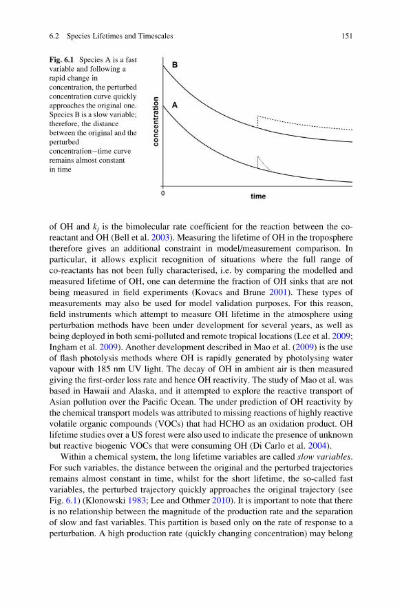
of OH and kj is the bimolecular rate coefficient for the reaction between the co-

reactant and OH (Bell et al. 2003). Measuring the lifetime of OH in the troposphere

therefore gives an additional constraint in model/measurement comparison. In

particular, it allows explicit recognition of situations where the full range of

co-reactants has not been fully characterised, i.e. by comparing the modelled and

measured lifetime of OH, one can determine the fraction of OH sinks that are not

being measured in field experiments (Kovacs and Brune 2001). These types of

measurements may also be used for model validation purposes. For this reason,

field instruments which attempt to measure OH lifetime in the atmosphere using

perturbation methods have been under development for several years, as well as

being deployed in both semi-polluted and remote tropical locations (Lee et al. 2009;

Ingham et al. 2009). Another development described in Mao et al. (2009) is the use

of flash photolysis methods where OH is rapidly generated by photolysing water

vapour with 185 nm UV light. The decay of OH in ambient air is then measured

giving the first-order loss rate and hence OH reactivity. The study of Mao et al. was

based in Hawaii and Alaska, and it attempted to explore the reactive transport of

Asian pollution over the Pacific Ocean. The under prediction of OH reactivity by

the chemical transport models was attributed to missing reactions of highly reactive

volatile organic compounds (VOCs) that had HCHO as an oxidation product. OH

lifetime studies over a US forest were also used to indicate the presence of unknown

but reactive biogenic VOCs that were consuming OH (Di Carlo et al. 2004).

Within a chemical system, the long lifetime variables are called slow variables.For such variables, the distance between the original and the perturbed trajectories

remains almost constant in time, whilst for the short lifetime, the so-called fast

variables, the perturbed trajectory quickly approaches the original trajectory (see

Fig. 6.1) (Klonowski 1983; Lee and Othmer 2010). It is important to note that there

is no relationship between the magnitude of the production rate and the separation

of slow and fast variables. This partition is based only on the rate of response to a

perturbation. A high production rate (quickly changing concentration) may belong

Fig. 6.1 Species A is a fast

variable and following a

rapid change in

concentration, the perturbed

concentration curve quickly

approaches the original one.

Species B is a slow variable;

therefore, the distance

between the original and the

perturbed

concentration�time curve

remains almost constant

in time


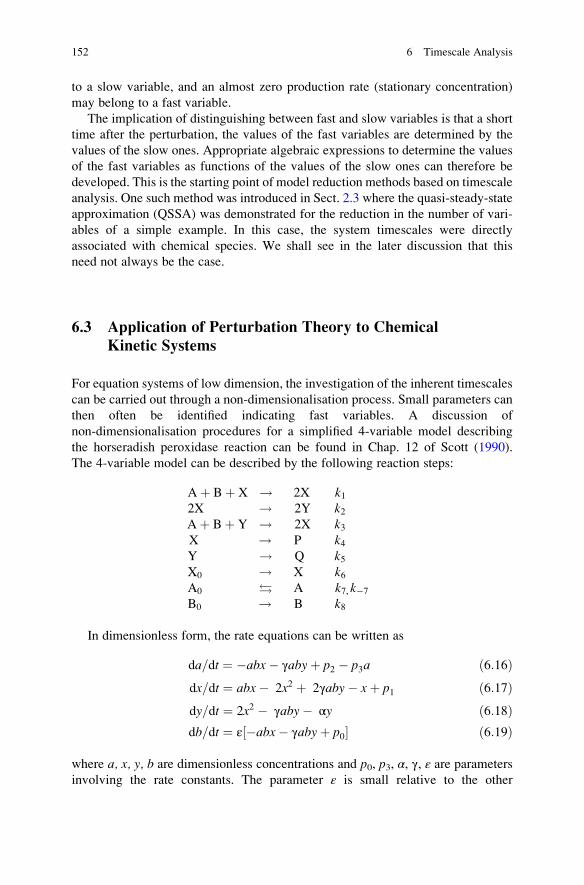
to a slow variable, and an almost zero production rate (stationary concentration)

may belong to a fast variable.

The implication of distinguishing between fast and slow variables is that a short

time after the perturbation, the values of the fast variables are determined by the

values of the slow ones. Appropriate algebraic expressions to determine the values

of the fast variables as functions of the values of the slow ones can therefore be

developed. This is the starting point of model reduction methods based on timescale

analysis. One such method was introduced in Sect. 2.3 where the quasi-steady-state

approximation (QSSA) was demonstrated for the reduction in the number of vari-

ables of a simple example. In this case, the system timescales were directly

associated with chemical species. We shall see in the later discussion that this

need not always be the case.

6.3 Application of Perturbation Theory to Chemical

Kinetic Systems

For equation systems of low dimension, the investigation of the inherent timescales

can be carried out through a non-dimensionalisation process. Small parameters can

then often be identified indicating fast variables. A discussion of

non-dimensionalisation procedures for a simplified 4-variable model describing

the horseradish peroxidase reaction can be found in Chap. 12 of Scott (1990).

The 4-variable model can be described by the following reaction steps:

Aþ Bþ X ! 2X k12X ! 2Y k2Aþ Bþ Y ! 2X k3X ! P k4Y ! Q k5X0 ! X k6A0 Æ A k7, k�7

B0 ! B k8

In dimensionless form, the rate equations can be written as

da=dt ¼ �abx� γabyþ p2 � p3a ð6:16Þdx=dt ¼ abx� 2x2 þ 2γaby� xþ p1 ð6:17Þdy=dt ¼ 2x2 � γaby� αy ð6:18Þdb=dt ¼ ε �abx� γabyþ p0½ � ð6:19Þ

where a, x, y, b are dimensionless concentrations and p0, p3, α, γ, ε are parameters

involving the rate constants. The parameter ε is small relative to the other



parameters and indicates that b will evolve on a slower timescale than the other

variables. The non-dimensionalisation procedure has therefore revealed a timescale

separation in this system which suggests that the system can be decoupled into a

“fast” 3-variable subset (a,x,y) and a slowly evolving variable b.For larger systems such as those typically found in complex chemical problems,

non-dimensionalisation may be impractical, and hence, numerical perturbation

methods are generally used to investigate system dynamics and to explore timescale

separation. By studying the evolution of a small disturbance or perturbation to the

nonlinear system, it is possible to reduce the problem to a locally linear one. The

resulting set of linear equations is easier to solve, and information can be obtained

about the local timescales and stability of the nonlinear system. Several books on

mathematics and physics (see e.g. Pontryagin 1962) discuss the linear stability

analysis of the stationary states of a dynamical system. In this case, the dynamical

system, described by an ODE, is in stationary state, i.e. the values of its variables

are constant in time. If the stationary concentrations are perturbed, one of the

possible results is that the stationary state is asymptotically stable, which means

that the perturbed system always returns to the stationary state. Another possible

outcome is that the stationary point is unstable. In this case, it is possible that the

system returns to the stationary state after perturbation towards some special

directions but may permanently deviate after a perturbation to other directions. A

full discussion of stationary state analysis in chemical systems is given in

Scott (1990).

In the following paragraphs, a more complicated system will be investigated,

which is a generalisation of the stability analysis applied to stationary states. The

system we investigate is described by the ODE defined in Eq. (2.9), i.e. it is an

initial value problem where the concentrations are changing in time. We now ask

the following question: how will the system respond, if one or several concen-

trations are changed instantaneously at any point in time? This type of analysis can

be used to investigate inherent timescales within dynamical chemical systems, the

couplings between species, and to determine species which drive the slow, inter-

mediate and fast dynamics of the system (Tomlin et al. 2001).

Let us change the concentrations of several species during the course of the

reaction at an arbitrarily selected time t0¼ 0 according to the vector ΔY0:

eY 0ð Þ ¼ Y 0ð Þ þ ΔY0 ð6:20Þ

The vector of concentrations eY tð Þ at a later time t can be given as the sum of the

original concentrations Y(t) and the effect of the perturbation ΔY(t):

eY tð Þ ¼ Y tð Þ þ ΔY tð Þ ð6:21Þ

The time derivative of eY tð Þ can be calculated in two ways. For the first method

(a linearisation), a Taylor series expansion is used with higher-order terms

neglected:

6.3 Application of Perturbation Theory to Chemical Kinetic Systems 153

deYdt

¼ d Yþ ΔYð Þdt

� f Y; pð Þ þ ∂f∂Y

ΔY ¼ f Y; pð Þ þ JΔY ð6:22Þ

Alternatively, the derivative of the sum Y +ΔY is calculated as the sum of the

derivatives:

deYdt

¼ d Yþ ΔYð Þdt

¼ f Y; pð Þ þ dΔYd t

ð6:23Þ

The left-hand sides of Eqs. (6.22) and (6.23) are equal to each other, and therefore,

dΔYdt

¼ J ΔY ð6:24Þ

During very short time periods, the Jacobian does not change significantly (the

Jacobian J0¼ J(t0) is constant), and therefore, the differential equation (6.24) can

be solved analytically:

ΔY tð Þ ¼ eJ0 t ΔY0 ð6:25Þ

giving the change in concentration at time t due to the perturbation at time t0. We

are used to meeting exponential functions with scalar arguments in science,

whereas here J0 is a matrix. However, an exponential function can be defined as

a series of power functions. Since the product and sum of matrices can be

interpreted, the series of power functions can also be interpreted for matrices.

This series will be convergent for any matrix, and therefore, the exponential

function may have a matrix argument.

The first step in the calculation of the matrix exponential can be (Prasolov 1994)

the decomposition of matrix J0 to its Jordan canonical form J using the invertible

matrix P:

J0 ¼ PJP�1 ð6:26Þ

where

eJ0t ¼ PeJ tP�1 ð6:27Þ

The eigenvalue�eigenvector decomposition of matrix J0 is the following:

J0 ¼ VΛW ð6:28Þ

where matrix Λ is the diagonal matrix of eigenvalues (Λ¼ diag(λ1, . . ., λn)),matrix V contains the right eigenvectors as column vectors (V ¼ v1 . . . vn½ �)and matrix W¼V�1 contains the left eigenvectors as row vectors

(W ¼ w1 . . . wn½ �T).


The recent trend is that very large reaction mechanisms are created either

manually or automatically for the combustion or the atmospheric decomposition

of large organic molecules [see e.g. (Herbinet et al. 2010; Westbrook et al. 2011)],

as discussed in Sect. 3.1. In such mechanisms, only a minority of the reaction steps

has an experimentally measured rate coefficient, and most of the reaction para-

meters are estimated using simple rules. Therefore, it is common that many rate

coefficients are identical within such mechanisms. A numerical consequence can be

that an eigenvalue� eigenvector decomposition of the Jacobian does not exist.

However, even in this case, the effect of concentration perturbations can always

be studied on the basis of the Jordan decomposition of the Jacobian (Nagy and

Turanyi 2009), as discussed below.

The eigenvalues of a matrix may have algebraic and may have geometric

multiplicity (Prasolov 1994). The algebraic multiplicity a(λ) of eigenvalue λ is

equal to the multiplicity of root λ of the characteristic polynomial. The geometric

multiplicity g(λ) is equal to the dimension of the eigensubspace belonging to λ,i.e. equal to the number of linearly independent eigenvectors belonging to eigen-

value λ. An eigenvalue is called degenerate if g(λ)< a(λ). If at least one eigenvalueof matrix J0 is degenerate, then matrix J0 does not have an eigenvalue�eigenvector

decomposition corresponding to Eq. (6.28). However, in all cases, the Jacobian J0has a Jordan decomposition according to Eq. (6.26) (Nagy and Turanyi 2009b).

If the Jacobian can be diagonalised according to Eq. (6.28), much simpler

equations are obtained:

ΔY tð Þ ¼ eJ0 tΔY0 ¼Xnl¼1

eλl tvl wlΔY0� � ¼Xn

l¼1

eλl t vl∘wlð ÞΔY0

¼Xnl¼1

eλl tPlΔY0 ð6:29Þ

where vl is the l-th column of the right eigenvector matrix and wl is the l-th row of

the left eigenvector matrix. The projector matrix Pl can be calculated by the tensor

product (also called dyadic product or outer product) of vectors vl and wl.

The Jacobian is not a symmetric matrix, and therefore the eigenvalues can also

be complex numbers. Let us assume now that the eigenvalues have zero imaginary

components. Rewriting Eq. (6.29) to a form containing scalar valued functions

only, the concentration changes can be described by the sum of exponential

functions, where the arguments of the exponential functions contain the eigen-

values of the Jacobian. The number of eigenvalues is equal to the number of

variables, and each eigenvalue is associated with a different timescale of the locally

linear solution to the full equations. The eigenvalue with the largest negative real

part corresponds to a perturbation which decays very quickly and is therefore

associated with the fastest timescale. However, there is no one-to-one equivalence

between the eigenvalues and the variables (concentrations of species). For

nonlinear systems with species coupling, several different timescales may



contribute to the decay or growth of each species perturbation, and conversely

several different species may contribute to each timescale. The calculation of

eigenvectors is useful since the off-diagonal terms tell us about the couplings

between species and the contributions of individual species to different timescale

modes (see discussion below). In the general case, however, there is not necessarily

a direct connection between the rate of return after the perturbation and the lifetime

of an individual species defined by Eq. (6.11) as highlighted in the following

discussion.

If the concentration of a single species is changed byΔy0i so that the perturbationis small enough to induce a linear response (which means that the rate of return is

proportional to the extent of deviation), and so that the change in concentration of

the other species is negligible, then the return of the perturbed concentration can be

described by the following exponential function:

Δyi tð Þ ¼ Δy0i eJii t ð6:30Þ

If the perturbed species has a short lifetime (i.e. has a high reactivity), and there is

sufficient separation between the timescales, then the conditions above are usually

fulfilled. The concentrations of these species quickly return to the original trajec-

tory, and the return can be described by a single exponential function. In this case,

the exponent of the exponential is related [see Eq. (6.11)] to the lifetime of the

species.

If the concentrations of several species are perturbed simultaneously, it is still

possible that the return to the original trajectory is described by single exponential

function, if the direction of the perturbation is appropriate. According to the

diagonalisation of the Jacobian,

Λ ¼ WJ0V ð6:31Þ

whereW is the matrix of left eigenvectors (row vectors) and V is the matrix of right

eigenvectors (column vectors). This equation is equivalent to the previous

Eq. (6.28), since

WV ¼ VW ¼ I ð6:32Þ

and thus

J0 ¼ VΛW ð6:33Þ

where I is the identity matrix.

If the values of variables are changed by ΔY0j ¼ α vj, where α is a small scalar

and vj is the j-th column of matrix V (the j-th right eigenvector), then using

Eq. (6.29), the displacement of the values of variables from the original values as

a function of time can be calculated using the following equation:


ΔYj tð Þ ¼ ΔY0j e

λj t ð6:34Þ

This means that, according to a local linear approximation, the approach from

perturbation direction vj to the original trajectory can be characterised by a single

exponential function having parameter λj. The problem is that the Jacobian is not

symmetrical, and therefore, λj can be a complex number.

If λj is a real number (Im(λj)¼ 0), then in the space of concentrations, the point

characterising the actual state of the system is moving along the original trajectory,

and its distance from the trajectory is changing in time according to a real expo-

nential function. If λj is a real number (i.e. if λj¼Re(λj)), then the distance of the

perturbed system from the unperturbed one is exponentially decreasing (λj< 0), is

increasing (λj> 0) or remains constant (λj¼ 0).

If λj is a complex number (Im(λj) 6¼ 0), then the point is moving in a 2D subspace

defined by the real and imaginary parts of the complex eigenvector. This point is

moving with rotational frequency ω¼ Im(λj) (i.e. with period 2π/Im (λj)) in an

ellipse having axes with length exp(Re(λj) t). In the general case, the point of the

system follows an elliptic spiral along the trajectory of the original (unperturbed)

system. If λj is a complex number and its real part (Re(λj)) is negative, then the

average distance (i.e. average over a period) is decreasing with time. The approach

is faster, if Re(λj) is a lower negative number, i.e. if | Re(λj) | is larger and Re(λj) isnegative. If Re(λj) is zero, then the distance averaged over a period is constant. If Re(λj) is positive, then the average distance between the original and the perturbed

states is increasing and the increase is faster if Re(λj) is larger. The ratio 1/|Re(λj) | iscalled the j-th timescale of the dynamical system.

The dynamic behaviour of the system tends to be dominated by the motion

associated with either the positive eigenvalues or the smallest negative ones, since

those with large negative eigenvalues tend to relax to their local equilibria very

quickly and therefore do not influence the slower modes.

If a small amount of a species is added to a reacting mixture, the resulting higher

concentration may increase the rate of the consuming reactions. Consequently, the

difference between the old and new concentration trajectory diminishes. This case

is associated with the presence of negative eigenvalues. If the behaviour of the

system is controlled by an autocatalytic species, then adding the autocatalyst

induces changes that further increase the concentration of the autocatalyst. A

similar behaviour is found when the added species can be converted quickly to

the autocatalyst. In such systems, the Jacobian has at least one positive Re(λj). Forexample, in explosions, the highest eigenvalue of the Jacobian is positive during

rapid changes of the concentrations, whilst the real parts of all eigenvalues are

negative before and after this period.

A systematic investigation of explosions based on the eigenanalysis of the

Jacobian is called chemical explosive mode analysis (CEMA) (Lu et al. 2010;

Luo et al. 2012c). An explosion index is defined for the explosive modes, which

is similar to the radical pointer of the CSP method discussed below. This indicates


the contribution of the various species and temperature to the explosion process and

thus facilitates the distinction between radical and thermal runaways.

It is clear that, based on small perturbations of concentrations, lifetimes can be

related to chemical kinetic systems. These lifetimes do not belong to species,

however, but to combinations of species concentrations defined by the left eigen-

vectors of the Jacobian, called modes. A matrix Jacobian of size NS�NS has NS

eigenvalues, and therefore, the number of modes is identical to the number of

variables. In the case of a linear system (in reaction kinetics, this means that the

mechanism consists of first-order and zeroth-order reactions only), the Jacobian is

constant and does not depend on the values of variables (concentrations). If the

system is nonlinear, which is the case for most reaction kinetic systems, the

Jacobian depends on the values of variables, i.e. the timescales depend on

the concentrations. In other words, the set of timescales belong to a given point in

the space of concentrations (phase space) and are different from location to location

(or from time point to time point if the concentrations change in time).

As Eq. (6.34) shows, concentration perturbations along the directions of the right

eigenvectors of the Jacobian have special importance. Therefore, it is justified to

introduce a new coordinate system. It is called the space of modes, and its axes are

defined by the eigenvectors. Using the left eigenvectors of the Jacobian, a concen-

tration set (point in the space of concentrations) can always be converted to a point

in the space of modes. The vector of modes z can be calculated using the following

equation:

z ¼ W Y ð6:35Þ

The i-th mode coordinate is

zi ¼ wi Y ð6:36Þ

Knowing the vector of modes, the concentration vector (or concentration yi) can becalculated:

Y ¼ V z ð6:37Þyi ¼ vi z ð6:38Þ

The initial value problem (2.9) has been used for the calculation of concentration

changes in time. A similar initial value problem can be used to calculate the change

of modes z in time:

dz

dt¼ W f Vzð Þ, z0 ¼ W Y0 ð6:39Þ

Since the Jacobian depends on the concentrations for nonlinear chemical kinetic

equations, the transformations above are also different at different points in the

concentration space.


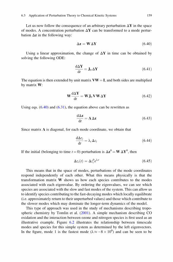
Let us now follow the consequence of an arbitrary perturbation ΔY in the space

of modes. A concentration perturbation ΔY can be transformed to a mode pertur-

bation Δz in the following way:

Δz ¼ WΔY ð6:40Þ

Using a linear approximation, the change of ΔY in time can be obtained by

solving the following ODE:

dΔYdt

¼ J0ΔY ð6:41Þ

The equation is then extended by unit matrix VW¼ I, and both sides are multiplied

by matrix W:

WdΔYdt

¼ WJ0VWΔY ð6:42Þ

Using eqs. (6.40) and (6.31), the equation above can be rewritten as

dΔzdt

¼ ΛΔz ð6:43Þ

Since matrix Λ is diagonal, for each mode coordinate, we obtain that

dΔzidt

¼ λiΔzi ð6:44Þ

If the initial (belonging to time t¼ 0) perturbation is Δz0¼WΔY0, then

Δzi tð Þ ¼ Δz0i eλit ð6:45Þ

This means that in the space of modes, perturbations of the mode coordinates

respond independently of each other. What this means physically is that the

transformation matrix W shows us how each species contributes to the modes

associated with each eigenvalue. By ordering the eigenvalues, we can see which

species are associated with the slow and fast modes of the system. This can allow us

to identify species contributing to the fast-decaying modes which locally equilibrate

(i.e. approximately return to their unperturbed values) and those which contribute to

the slower modes which may dominate the longer-term dynamics of the model.

This type of approach was used in the study of mechanisms describing tropo-

spheric chemistry by Tomlin et al. (2001). A simple mechanism describing CO

oxidation and the interaction between ozone and nitrogen species is first used as an

illustrative example. Figure 6.2 illustrates the relationship between timescale

modes and species for this simple system as determined by the left eigenvectors.

In the figure, mode 1 is the fastest mode (λ��8� 108) and can be seen to be


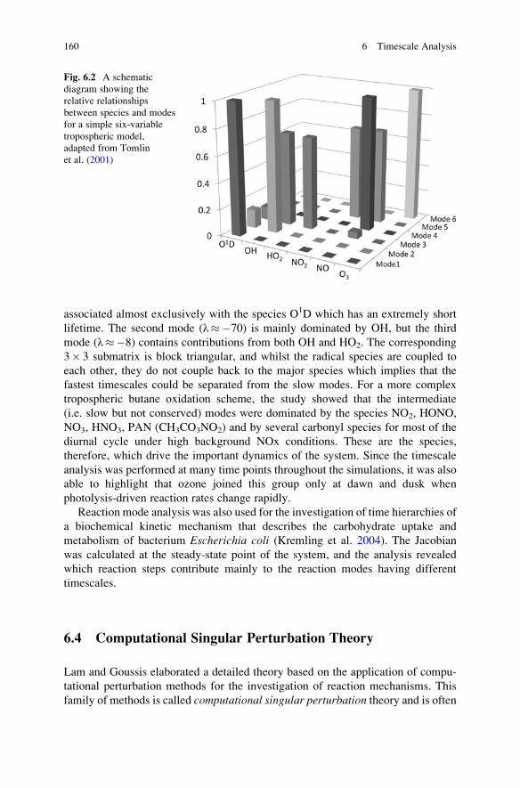
associated almost exclusively with the species O1D which has an extremely short

lifetime. The second mode (λ��70) is mainly dominated by OH, but the third

mode (λ��8) contains contributions from both OH and HO2. The corresponding

3� 3 submatrix is block triangular, and whilst the radical species are coupled to

each other, they do not couple back to the major species which implies that the

fastest timescales could be separated from the slow modes. For a more complex

tropospheric butane oxidation scheme, the study showed that the intermediate

(i.e. slow but not conserved) modes were dominated by the species NO2, HONO,

NO3, HNO3, PAN (CH3CO3NO2) and by several carbonyl species for most of the

diurnal cycle under high background NOx conditions. These are the species,

therefore, which drive the important dynamics of the system. Since the timescale

analysis was performed at many time points throughout the simulations, it was also

able to highlight that ozone joined this group only at dawn and dusk when

photolysis-driven reaction rates change rapidly.

Reaction mode analysis was also used for the investigation of time hierarchies of

a biochemical kinetic mechanism that describes the carbohydrate uptake and

metabolism of bacterium Escherichia coli (Kremling et al. 2004). The Jacobian

was calculated at the steady-state point of the system, and the analysis revealed

which reaction steps contribute mainly to the reaction modes having different

timescales.

6.4 Computational Singular Perturbation Theory

Lam and Goussis elaborated a detailed theory based on the application of compu-

tational perturbation methods for the investigation of reaction mechanisms. This

family of methods is called computational singular perturbation theory and is often

Fig. 6.2 A schematic

diagram showing the

relative relationships

between species and modes

for a simple six-variable

tropospheric model,

adapted from Tomlin

et al. (2001)


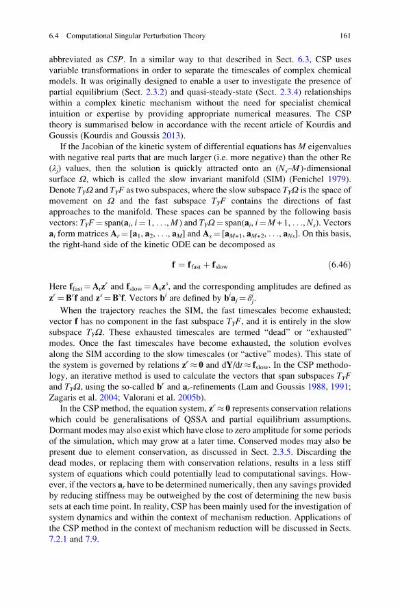
abbreviated as CSP. In a similar way to that described in Sect. 6.3, CSP uses

variable transformations in order to separate the timescales of complex chemical

models. It was originally designed to enable a user to investigate the presence of

partial equilibrium (Sect. 2.3.2) and quasi-steady-state (Sect. 2.3.4) relationships

within a complex kinetic mechanism without the need for specialist chemical

intuition or expertise by providing appropriate numerical measures. The CSP

theory is summarised below in accordance with the recent article of Kourdis and

Goussis (Kourdis and Goussis 2013).

If the Jacobian of the kinetic system of differential equations has M eigenvalues

with negative real parts that are much larger (i.e. more negative) than the other Re

(λj) values, then the solution is quickly attracted onto an (Ns–M )-dimensional

surface Ω, which is called the slow invariant manifold (SIM) (Fenichel 1979).

Denote TYΩ and TYF as two subspaces, where the slow subspace TYΩ is the space of

movement on Ω and the fast subspace TYF contains the directions of fast

approaches to the manifold. These spaces can be spanned by the following basis

vectors: TYF¼ span(ai, i¼ 1, . . .,M ) and TYΩ¼ span(ai, i¼M+ 1, . . ., Ns). Vectors

ai form matrices Ar¼ [a1, a2, . . ., aM] and As¼ [aM+1, aM+2, . . ., aNs]. On this basis,the right-hand side of the kinetic ODE can be decomposed as

f ¼ f fast þ fslow ð6:46Þ

Here ffast¼Arzr and fslow¼Asz

s, and the corresponding amplitudes are defined as

zr¼Brf and zs¼Bsf. Vectors bi are defined by biaj¼ δij.

When the trajectory reaches the SIM, the fast timescales become exhausted;

vector f has no component in the fast subspace TYF, and it is entirely in the slow

subspace TYΩ. These exhausted timescales are termed “dead” or “exhausted”

modes. Once the fast timescales have become exhausted, the solution evolves

along the SIM according to the slow timescales (or “active” modes). This state of

the system is governed by relations zr� 0 and dY/dt� fslow. In the CSP methodo-

logy, an iterative method is used to calculate the vectors that span subspaces TYFand TYΩ, using the so-called b

r and ar-refinements (Lam and Goussis 1988, 1991;

Zagaris et al. 2004; Valorani et al. 2005b).

In the CSP method, the equation system, zr� 0 represents conservation relations

which could be generalisations of QSSA and partial equilibrium assumptions.

Dormant modes may also exist which have close to zero amplitude for some periods

of the simulation, which may grow at a later time. Conserved modes may also be

present due to element conservation, as discussed in Sect. 2.3.5. Discarding the

dead modes, or replacing them with conservation relations, results in a less stiff

system of equations which could potentially lead to computational savings. How-

ever, if the vectors ar have to be determined numerically, then any savings provided

by reducing stiffness may be outweighed by the cost of determining the new basis

sets at each time point. In reality, CSP has been mainly used for the investigation of

system dynamics and within the context of mechanism reduction. Applications of

the CSP method in the context of mechanism reduction will be discussed in Sects.

7.2.1 and 7.9.

6.4 Computational Singular Perturbation Theory 161






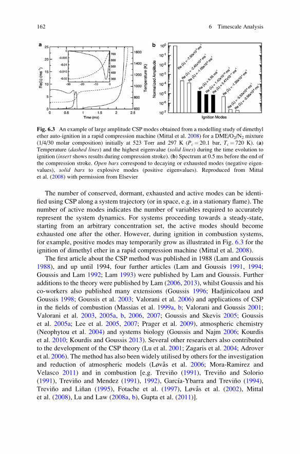
The number of conserved, dormant, exhausted and active modes can be identi-

fied using CSP along a system trajectory (or in space, e.g. in a stationary flame). The

number of active modes indicates the number of variables required to accurately

represent the system dynamics. For systems proceeding towards a steady-state,

starting from an arbitrary concentration set, the active modes should become

exhausted one after the other. However, during ignition in combustion systems,

for example, positive modes may temporarily grow as illustrated in Fig. 6.3 for the

ignition of dimethyl ether in a rapid compression machine (Mittal et al. 2008).

The first article about the CSP method was published in 1988 (Lam and Goussis

1988), and up until 1994, four further articles (Lam and Goussis 1991, 1994;

Goussis and Lam 1992; Lam 1993) were published by Lam and Goussis. Further

additions to the theory were published by Lam (2006, 2013), whilst Goussis and his

co-workers also published many extensions (Goussis 1996; Hadjinicolaou and

Goussis 1998; Goussis et al. 2003; Valorani et al. 2006) and applications of CSP

in the fields of combustion (Massias et al. 1999a, b; Valorani and Goussis 2001;

Valorani et al. 2003, 2005a, b, 2006, 2007; Goussis and Skevis 2005; Goussis

et al. 2005a; Lee et al. 2005, 2007; Prager et al. 2009), atmospheric chemistry

(Neophytou et al. 2004) and systems biology (Goussis and Najm 2006; Kourdis

et al. 2010; Kourdis and Goussis 2013). Several other researchers also contributed

to the development of the CSP theory (Lu et al. 2001; Zagaris et al. 2004; Adrover

et al. 2006). The method has also been widely utilised by others for the investigation

and reduction of atmospheric models (Løvas et al. 2006; Mora-Ramirez and

Velasco 2011) and in combustion [e.g. Trevino (1991), Trevino and Solorio

(1991), Trevino and Mendez (1991), 1992), Garcıa-Ybarra and Trevino (1994),

Trevino and Linan (1995), Fotache et al. (1997), Løvas et al. (2002), Mittal

et al. (2008), Lu and Law (2008a, b), Gupta et al. (2011)].

Fig. 6.3 An example of large amplitude CSP modes obtained from a modelling study of dimethyl

ether auto-ignition in a rapid compression machine (Mittal et al. 2008) for a DME/O2/N2 mixture

(1/4/30 molar composition) initially at 523 Torr and 297 K (Pc¼ 20.1 bar, Tc¼ 720 K). (a)

Temperature (dashed lines) and the highest eigenvalue (solid lines) during the time evolution to

ignition (insert shows results during compression stroke). (b) Spectrum at 0.5 ms before the end of

the compression stroke. Open bars correspond to decaying or exhausted modes (negative eigen-

values), solid bars to explosive modes (positive eigenvalues). Reproduced from Mittal

et al. (2008) with permission from Elsevier


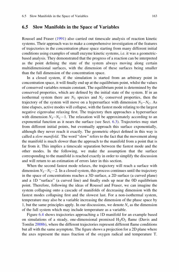
6.5 Slow Manifolds in the Space of Variables

Roussel and Fraser (1991) also carried out timescale analysis of reaction kinetic

systems. Their approach was to make a comprehensive investigation of the features

of trajectories in the concentration phase space starting from many different initial

conditions using examples of small enzyme kinetic systems, i.e. it was a geometric-

based analysis. They demonstrated that the progress of a reaction can be interpreted

as the point defining the state of the system always moving along certain

multidimensional surfaces, with the dimension of these surfaces being smaller

than the full dimension of the concentration space.

In a closed system, if the simulation is started from an arbitrary point in

concentration space, it will finally end up at the equilibrium point, whilst the values

of conserved variables remain constant. The equilibrium point is determined by the

conserved properties, which are defined by the initial state of the system. If in an

isothermal system there are NS species and NC conserved properties, then the

trajectory of the system will move on a hypersurface with dimension NS�NC. As

time elapses, active modes will collapse, with the fastest mode relating to the largest

negative eigenvalue relaxing first. The trajectory then approaches a hypersurface

with dimension NS�NC�1. The relaxation will be approximately according to an

exponential function as it nears the surface (see Sect. 6.3). Trajectories may start

from different initial points, but eventually approach this surface exponentially,

although they never reach it exactly. The geometric object defined in this way is

called a slow manifold. The word “slow” refers to the fact that the movement along

the manifold is much slower than the approach to the manifold from a point that is

far from it. This implies a timescale separation between the fastest mode and the

other modes. In the following, we make the assumption that the surface

corresponding to the manifold is reached exactly in order to simplify the discussion

and will return to an estimation of errors later in this section.

When the second fastest mode relaxes, the trajectory will reach a surface with

dimension NS�NC�2. In a closed system, this process continues until the trajectory

in the space of concentrations reaches a 3D surface, a 2D surface (a curved plane)

and a 1D “surface” (a curved line) and finally ends up near the 0D equilibrium

point. Therefore, following the ideas of Roussel and Fraser, we can imagine the

system collapsing onto a cascade of manifolds of decreasing dimension with the

fastest modes collapsing first and the slowest last. For a non-isothermal system,

temperature may also be a variable increasing the dimension of the phase space by

1, but the same principles apply. In our discussions, we denote Ns as the dimension

of the full system which may include temperature as a variable.

Figure 6.4 shows trajectories approaching a 1D manifold for an example based

on simulations of a steady, one-dimensional premixed H2/O2 flame (Davis and

Tomlin 2008b), where the different trajectories represent different flame conditions

but all with the same asymptote. The figure shows a projection for a 2D plane where

the axes represent the mass fraction of the oxygen radical and temperature T.

6.5 Slow Manifolds in the Space of Variables 163

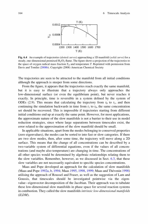
The trajectories are seen to be attracted to the manifold from all initial conditions

although the approach is steeper from some directions.

From the figure, it appears that the trajectories reach exactly the same manifold,

but it is easy to illustrate that a trajectory always only approaches the

low-dimensional surface (or even the equilibrium point), but never reaches it

exactly. In principle, time is reversible in a system defined by the system of

ODEs (2.9). This means that calculating the trajectory from t0 to t1, and then

continuing the simulation backwards in time from t1 to t0, the same concentration

set should be recovered. This is impossible if trajectories starting from different

initial conditions end up at exactly the same point. However, for most applications,

the approximate nature of the slow manifolds is not a barrier to their use in model

reduction strategies, since where large separations between timescales exist, the

error related to the approximation of the slow manifold should be small.

In applicable situations, apart from the modes belonging to conserved properties

(zero eigenvalues), the modes can be sorted to into fast or slow categories. If there

are two slow modes, then, after some time, the trajectory will move along a 2D

surface. This means that the change of all concentrations can be described by a

two-variable system of differential equations, even if the values of all concen-

trations (and maybe also temperature) are changing in time. The concentrations of

all other species would be determined by algebraic relationships relating them to

the slow variables. Remember, however, as we discussed in Sect. 6.3, that these

slow variables are not necessarily equivalent to specific species concentrations.

Maas and Pope developed an approach for the calculation of slow manifolds

(Maas and Pope 1992a, b, 1994; Maas 1995, 1998, 1999; Maas and Thevenin 1998)

utilising the approach of Roussel and Fraser, as well as the suggestion of Lam and

Goussis, that timescales should be investigated pointwise via the eigen-

value�eigenvector decomposition of the Jacobian. Their approach was to tabulate

these low-dimensional slow manifolds in phase space for several reaction systems

in combustion. They called the slow manifolds intrinsic low-dimensional manifolds(ILDM).

Fig. 6.4 An example of trajectories (dotted curves) approaching a 1D manifold (solid curve) for asteady, one-dimensional premixed H2/O2 flame. The figure shows a projection of the trajectories to

the space of oxygen radical mass fraction YO and temperature T. Reprinted with permission from

Davis and Tomlin (2008b). Copyright (2008) American Chemical Society


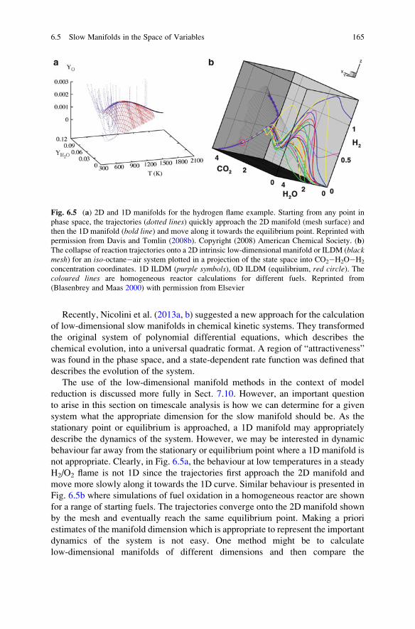
Recently, Nicolini et al. (2013a, b) suggested a new approach for the calculation

of low-dimensional slow manifolds in chemical kinetic systems. They transformed

the original system of polynomial differential equations, which describes the

chemical evolution, into a universal quadratic format. A region of “attractiveness”

was found in the phase space, and a state-dependent rate function was defined that

describes the evolution of the system.

The use of the low-dimensional manifold methods in the context of model

reduction is discussed more fully in Sect. 7.10. However, an important question

to arise in this section on timescale analysis is how we can determine for a given

system what the appropriate dimension for the slow manifold should be. As the

stationary point or equilibrium is approached, a 1D manifold may appropriately

describe the dynamics of the system. However, we may be interested in dynamic

behaviour far away from the stationary or equilibrium point where a 1D manifold is

not appropriate. Clearly, in Fig. 6.5a, the behaviour at low temperatures in a steady

H2/O2 flame is not 1D since the trajectories first approach the 2D manifold and

move more slowly along it towards the 1D curve. Similar behaviour is presented in

Fig. 6.5b where simulations of fuel oxidation in a homogeneous reactor are shown

for a range of starting fuels. The trajectories converge onto the 2D manifold shown

by the mesh and eventually reach the same equilibrium point. Making a priori

estimates of the manifold dimension which is appropriate to represent the important

dynamics of the system is not easy. One method might be to calculate

low-dimensional manifolds of different dimensions and then compare the

Fig. 6.5 (a) 2D and 1D manifolds for the hydrogen flame example. Starting from any point in

phase space, the trajectories (dotted lines) quickly approach the 2D manifold (mesh surface) and

then the 1D manifold (bold line) and move along it towards the equilibrium point. Reprinted with

permission from Davis and Tomlin (2008b). Copyright (2008) American Chemical Society. (b)

The collapse of reaction trajectories onto a 2D intrinsic low-dimensional manifold or ILDM (blackmesh) for an iso-octane�air system plotted in a projection of the state space into CO2�H2O�H2

concentration coordinates. 1D ILDM (purple symbols), 0D ILDM (equilibrium, red circle). Thecoloured lines are homogeneous reactor calculations for different fuels. Reprinted from

(Blasenbrey and Maas 2000) with permission from Elsevier



behaviour of the system on these manifolds to trajectories calculated from the full

model. This could be time consuming, however, and hence, approaches have been

developed which attempt to estimate the dimension of the manifold along trajec-

tories based on the analysis of timescale modes. The method of Tomlin et al. (2001)

is based on ordering the eigenvalues for each of the timescale modes and investi-

gating their collapse onto an (Ns-1)-dimensional manifold in an Ns-dimensional

phase space. The dimension calculated this way is in good agreement with the

results of alternative methods for the determination of dynamical dimension (Buki

et al. 2002; Zsely et al. 2005). Valorani et al. (see Eq. (8) in Valorani et al. (2006))

derived a similar equation based on a CSP reasoning.

A consequence of Eqs. (6.25) and (6.44) is that the change of mode i after aperturbation can be described by the following equation:

dzidt

¼ wif ¼ wif Ymð Þ þ widΔYdt

¼ dΔzidt

ð6:47Þ

where wif(Ym)¼ 0, if point Ym is on the “surface” of the manifold, since the

direction of the movement f is always perpendicular to the surface spanned by

the vectors wi. Here Δzi denotes the size of perturbation along mode i and thereforegives a measure of the distance of the mode from its associated slow manifold.

By comparing Eqs. (6.44) and (6.47), we get

wif ¼ λiΔzi ð6:48Þ

The distance of the system from the slow manifold towards direction i can thereforebe calculated from

Δzi ¼ wif=λi ð6:49Þ

This gives only the relative distance since the choice of eigenvectors is not

unique and will affect the absolute value. By normalising we can obtain a measure

of the relative distance of each mode from its equivalent slow manifold:

Δezi ¼ wif=λi1

κ þ wiYj j ð6:50Þ

where κ is a small parameter added to avoid division by zero. This calculated

Δezi distance is not expected to become exactly zero since the trajectory only

approaches the manifold and can never be exactly on the corresponding surface.

However, we can define a threshold zth and state that the actual point has relaxed

to the slow manifold if��Δezi�� < zth. By estimating the distance of the system

according to the fastest mode from the corresponding Ns�1-dimensional manifold

and comparing it against a tolerance parameter, we can determine at each time

point along a trajectory if the fastest mode has effectively been collapsed. It also

follows that once the fastest mode has collapsed, then the error of assuming an


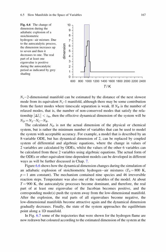
Ns�2-dimensional manifold can be estimated by the distance of the next slowest

mode from its equivalent Ns–1 manifold, although there may be some contribution

from the faster modes where timescale separation is weak. If NR is the number of

relaxed modes, that is, the number of non-conserved modes that satisfy the rela-

tionship��Δezi�� < zth, then the effective dynamical dimension of the system will be

ND¼NS�NC�NR.

The calculated ND is not the actual dimension of the physical or chemical

system, but is rather the minimum number of variables that can be used to model

the system with acceptable accuracy. For example, a model that is described by an

8-variable ODE, but has dynamical dimension of 2, can be replaced by coupled

system of differential and algebraic equations, where the change in values of

2 variables are calculated by ODEs, whilst the values of the other 6 variables can

be calculated from these 2 variables using algebraic equations. The actual form of

the ODEs or other equivalent time-dependent models can be developed in different

ways as will be further discussed in Chap. 7.

Figure 6.6 shows how the dynamical dimension changes during the simulation of

an adiabatic explosion of stoichiometric hydrogen�air mixtures (T0¼ 800 K,

p¼ 1 atm constant). The mechanism contained nine species and 46 irreversible

reaction steps. Temperature was also one of the variables of the model. At about

T¼ 900 K, the autocatalytic processes become dominant, and therefore, the real

part of at least one eigenvalue of the Jacobian becomes positive, and the

corresponding mode(s) push the system away from the low-dimensional manifold.

After the explosion, the real parts of all eigenvalues become negative, the

low-dimensional manifolds become attractive again and the dynamical dimension

gradually decreases. Finally, the state of the system approaches the equilibrium

point along a 1D manifold.

In Fig. 6.7 some of the trajectories that were shown for the hydrogen flame are

now redrawn but coloured according to the estimated dimension of the system at the

600 800 1000 1200 1400 1600 1800 2000 2200 2400012

34567

89

10

T / K

dim

ensi

on

Fig. 6.6 The change of

dimension during the

adiabatic explosion of a

stoichiometric

hydrogen�air mixture. Due

to the autocatalytic process,

the dimension increases up

to seven and then it

decreases to one. The real

part of at least one

eigenvalue is positive

during the autocatalytic

period as indicated by grey

shading


http://dx.doi.org/10.1007/978-3-662-44562-4_7

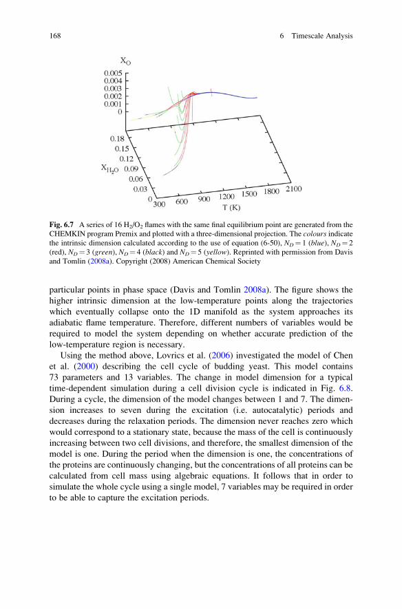
particular points in phase space (Davis and Tomlin 2008a). The figure shows the

higher intrinsic dimension at the low-temperature points along the trajectories

which eventually collapse onto the 1D manifold as the system approaches its

adiabatic flame temperature. Therefore, different numbers of variables would be

required to model the system depending on whether accurate prediction of the

low-temperature region is necessary.

Using the method above, Lovrics et al. (2006) investigated the model of Chen

et al. (2000) describing the cell cycle of budding yeast. This model contains

73 parameters and 13 variables. The change in model dimension for a typical

time-dependent simulation during a cell division cycle is indicated in Fig. 6.8.

During a cycle, the dimension of the model changes between 1 and 7. The dimen-

sion increases to seven during the excitation (i.e. autocatalytic) periods and

decreases during the relaxation periods. The dimension never reaches zero which

would correspond to a stationary state, because the mass of the cell is continuously

increasing between two cell divisions, and therefore, the smallest dimension of the

model is one. During the period when the dimension is one, the concentrations of

the proteins are continuously changing, but the concentrations of all proteins can be

calculated from cell mass using algebraic equations. It follows that in order to

simulate the whole cycle using a single model, 7 variables may be required in order

to be able to capture the excitation periods.

Fig. 6.7 A series of 16 H2/O2 flames with the same final equilibrium point are generated from the

CHEMKIN program Premix and plotted with a three-dimensional projection. The colours indicatethe intrinsic dimension calculated according to the use of equation (6-50), ND¼ 1 (blue), ND¼ 2

(red), ND¼ 3 (green), ND¼ 4 (black) and ND¼ 5 (yellow). Reprinted with permission from Davis

and Tomlin (2008a). Copyright (2008) American Chemical Society


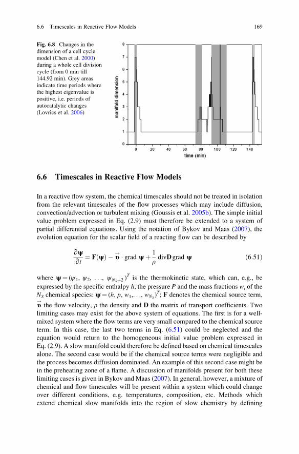
6.6 Timescales in Reactive Flow Models

In a reactive flow system, the chemical timescales should not be treated in isolation

from the relevant timescales of the flow processes which may include diffusion,

convection/advection or turbulent mixing (Goussis et al. 2005b). The simple initial

value problem expressed in Eq. (2.9) must therefore be extended to a system of

partial differential equations. Using the notation of Bykov and Maas (2007), the

evolution equation for the scalar field of a reacting flow can be described by

∂ψ∂t

¼ F ψð Þ � υ! � grad ψþ 1

ρdivDgrad ψ ð6:51Þ

where ψ¼ (ψ1, ψ2, . . ., ψNSþ2 )T is the thermokinetic state, which can, e.g., be

expressed by the specific enthalpy h, the pressure P and the mass fractions wi of the

NS chemical species: ψ¼ (h, p, w1,. . ., wNS)T; F denotes the chemical source term,

υ! the flow velocity, ρ the density and D the matrix of transport coefficients. Two

limiting cases may exist for the above system of equations. The first is for a well-

mixed system where the flow terms are very small compared to the chemical source

term. In this case, the last two terms in Eq. (6.51) could be neglected and the

equation would return to the homogeneous initial value problem expressed in

Eq. (2.9). A slow manifold could therefore be defined based on chemical timescales

alone. The second case would be if the chemical source terms were negligible and

the process becomes diffusion dominated. An example of this second case might be

in the preheating zone of a flame. A discussion of manifolds present for both these

limiting cases is given in Bykov and Maas (2007). In general, however, a mixture of

chemical and flow timescales will be present within a system which could change

over different conditions, e.g. temperatures, composition, etc. Methods which

extend chemical slow manifolds into the region of slow chemistry by defining

Fig. 6.8 Changes in the

dimension of a cell cycle

model (Chen et al. 2000)

during a whole cell division

cycle (from 0 min till

144.92 min). Grey areas

indicate time periods where

the highest eigenvalue is

positive, i.e. periods of

autocatalytic changes

(Lovrics et al. 2006)

6.6 Timescales in Reactive Flow Models 169

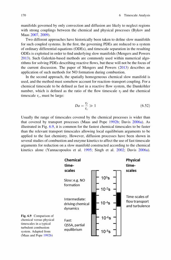
manifolds governed by only convection and diffusion are likely to neglect regions

with strong couplings between the chemical and physical processes (Bykov and

Maas 2007, 2009).

Two different approaches have historically been taken to define slow manifolds

for such coupled systems. In the first, the governing PDEs are reduced to a system

of ordinary differential equations (ODEs), and timescale separation in the resulting

ODEs is exploited in order to find underlying slow manifolds (Mengers and Powers

2013). Such Galerkin-based methods are commonly used within numerical algo-

rithms for solving PDEs describing reactive flows, but these will not be the focus of

the current discussion. The paper of Mengers and Powers (2013) describes an

application of such methods for NO formation during combustion.

In the second approach, the spatially homogeneous chemical slow manifold is

used, and the method must somehow account for reaction–transport coupling. For a

chemical timescale to be defined as fast in a reactive flow system, the Damkohler

number, which is defined as the ratio of the flow timescale τf and the chemical

timescale τc, must be large:

Da ¼ τfτc

� 1 ð6:52Þ

Usually the range of timescales covered by the chemical processes is wider than

that covered by transport processes (Maas and Pope 1992b; Davis 2006a). As

illustrated in Fig. 6.9, it is common for the fastest chemical timescales to be faster

than the relevant transport timescales allowing local equilibrium arguments to be

applied to the fast chemistry. However, diffusion processes have been shown in

several studies of combustion and enzyme kinetics to affect the use of fast timescale

arguments for reduction on a slow manifold constructed according to the chemical

kinetics alone (Yannacopoulos et al. 1995; Singh et al. 2002; Davis 2006a).

Fig. 6.9 Comparison of

chemical versus physical

timescales in a typical

turbulent combustion

system. Adapted from

(Maas and Pope 1992b)


The coupling of some chemical modes with relatively fast physical ones may

disturb system trajectories from the low-dimensional manifold (Bykov and Maas

2007). Prufert et al. (2014) provide a discussion of the comparison of species

lifetimes τi (see Eq. (6.11)), system timescales based on eigenvalues and two

additional timescales called system progress and progress variable timescales for

reactive flow models.

Yannacopoulos et al. (1995) showed for an enzyme kinetics reaction–diffusion

model that because of the spatial dependence of the solution in PDE systems, the

transient dynamics before relaxation to the slow chemical manifold can have a very

important effect on the solution at long times. The use of a singular perturbation

method for the approximation of the transient approach to the slow manifold was

seen to improve the simulation of the long-term dynamics of the reaction–diffusion

model. A higher-order approximation than the QSSA was also required in order to

approximate the slow manifold in this case. Davis et al. (Davis 2006a, b) also

showed that the presence of diffusion can affect the attractiveness of the slow

manifolds present in a reaction–diffusion model of ozone combustion. The situation

for turbulent systems may be even more complex since in such cases rapidly

changing transient flows may need to be captured by the reactive flow model.

However, Van Oijen et al. (2007) have applied slow manifold techniques even in

direct numerical simulations (DNS) of flames. They noted, however, that the 2D

slow manifold generated for the flame differed substantially from the one generated

based on the chemical kinetics alone. Davis and Tomlin (2008b) also noted

differences between the flame manifolds and those based on only chemical kinetics

for a hydrogen oxygen flame, when sufficiently far from the final equilibrium point.

These differences have been attributed to the influence of the non-invariance of the

manifold, the curvature of the manifold (for nonzero diffusion cases), differential

diffusion of the species (Ren and Pope 2006) and thermal diffusion (Maas and

Bykov 2011). It could be possible to solve such problems by using higher-

dimensional chemical manifolds, i.e. only collapsing those timescales which are

much faster than the transport ones, but this is not optimal from the point of view of

reducing the number of variables to solve for in a reduced model. Therefore, more

general approaches have been sought for the application of slow manifolds within

reaction–diffusion systems. These include the reaction–diffusion manifold

(REDIM) method (Bykov and Maas 2009) and methods based on the extension

of composition space to include, for example, diffusive fluxes (Bongers et al. 2002).

Both of these approaches will be discussed further in the context of model reduction

in Sect. 7.10.

6.7 Stiffness of Reaction Kinetic Models

One of the first applications of computers in science was the simulation of the

dislocation of weights interconnected with springs. When the springs were not stiff,

the simulation was easy and no numerical problems were encountered. However,

6.7 Stiffness of Reaction Kinetic Models 171


when some springs were loose and the others stiff, the numerical solution was far

more difficult, since the ODE solution code only gave sensible results when

extremely short time steps were used (Burden and Faires 1993). Physicists called

such tasks stiff problems and the corresponding ODE was called a stiff system ofdifferential equations. It was subsequently discovered that very similar problems

occur not only for the simulation of mechanical problems but also for reaction

kinetic models.

The stiffness of a dynamical system can be characterised via its timescales.

Remember that the ratio 1/|Re(λj) | is called the j-th timescale of a dynamical system

(see Sect. 6.3). The most widely used stiffness index is the reciprocal of the shortesttimescale of the system:

L ¼ 1

mini

τi¼ max

i

1

τi¼ max

iReλij j ð6:53Þ

where λi is the i-th eigenvalue of the Jacobian of the ODE of the system. However, it

is only possible to judge if such a quantity is large or small by comparing it to

another quantity. The shortest timescale should therefore be compared to the

characteristic timescale of the system.

Each process has a characteristic timescale. This is the time period during which

important events occur that are of interest to us. For example, in the case of a

summer storm, the timescale of temperature change is a few hours. During a

summer holiday, the change of temperature is of interest over a few weeks, whilst

climatologists investigate the change of the average temperature of air for time-

scales of several thousand or even several million years. In these three cases, the

physical system is identical (the atmosphere of Earth), the same quantity (air

temperature) is investigated, but the characteristic timescales of the investigations

are different.

A model is called stiff if its characteristic time T is several orders of magnitude

(typically 8–12 orders of magnitude) longer than its shortest timescale. Stiffness

can be characterised by the following stiffness ratio:

S1 ¼ T

miniτi¼ LT ð6:54Þ

Another possibility is to calculate the ratio of the longest and shortest timescales of

the model:

S2 ¼max

iReλij j

mini

Reλij j ð6:55Þ

Of course, zero eigenvalues (originating from the conserved properties of the

model) should not be considered.


It is important to emphasise that stiffness belongs to a model and not to a

physical system. The same physical system can be described, with similar accuracy,

by a very stiff and a non-stiff model. Several mathematics books consider stiffness

ratio S2 as a good indicator for stiffness, but stiffness ratio S1 is a more realistic

characterisation of the stiffness of a physical model. Inserting descriptions of

processes that have timescales much longer than the characteristic timescale into

a model will not affect the simulations. For example, according to the pool chemicalapproximation (see Sect. 2.3), if the concentration of a species changes negligibly

during the simulation, it can be considered constant and the equations can be

simplified accordingly. It is clear that adding more, less reactive species to the

model (which changes S2 but not S1) does not cause much change. In general it may

be possible to treat the very slow timescales as approximately conserved variables

by applying a threshold ε (i.e. |Reλi|� ε) and therefore to remove these timescales

from the consideration of S2.Both stiffness ratios S1 and S2 can be decreased by eliminating very fast

processes from the model or by changing the corresponding differential equations

to algebraic equations. Several sections of the next chapter, dealing with mecha-

nism reduction, discuss methods to modify models so that the fast timescales are

eliminated, hence reducing the stiffness of the model, even though the solution of

the model on the characteristic timescale is almost identical to the original one.

Algorithms for the solution of differential equations can be sorted into many

categories, but an important feature from a practical point of view is whether

these are applicable for the simulation of stiff systems.

A simple rule of thumb is that explicit methods for the solution of ODEs give fastsolutions for each time step but are not always applicable for the solution of stiff

systems. If an explicit method is used for the simulation of a stiff system using large

time steps, the solution obtained is usually not sensible, giving oscillating outputs or

the overprediction of quantities. Accuracy and stability problems can be solved by

selecting extremely short time steps, but then the overall CPU time required

becomes much too long. Using implicit methods for the solution of ODEs requiresmuch more CPU time for each time step, but the solution is stable even when using

longer time steps.

Explicit methods calculate the solution to Eq. (2.9) at time t+Δ t knowing the

solution at time t using the following general equation:

Y tþ Δtð Þ ¼ F Y tð Þð Þ ð6:56Þ

The general equation for implicit methods contains the solution of the system at

both times t and t+Δ t:

G Y tþ Δtð Þ,Y tð Þð Þ ¼ 0 ð6:57Þ

Equation (6.57) is a nonlinear algebraic equation. Solving it at each time step Δ twould require much CPU time, and so it is converted to an approximate linear

algebraic equation.

6.7 Stiffness of Reaction Kinetic Models 173


When an explicit method is used, the solution Y at time t is fed into Eq. (6.56) toget the solution at time t+Δ t. Using an implicit method, the Jacobian has to be

evaluated at each time step, and then using this matrix, an N-variable linear

algebraic system of equations has to be solved. If using the same time step Δ t forboth methods, the implicit method will require more CPU time unless highly

efficient matrix algebra techniques can be employed. If the ODE is not stiff, then

both explicit and implicit methods give an accurate solution. If the ODE is stiff,

then the explicit method will not give sensible results for large time stepsΔ t, whilstthe implicit method may give an accurate numerical solution. This means that if the

ODE is not stiff, then it is usually not practical (although possible) to use an implicit

method. For the solution of a stiff ODE, it may be more practical to use an implicit

method, although the use of variable time steps can improve the efficiency of

explicit schemes (Sandu et al. 1997b).

A full discussion of the issues involved and comparisons between the appli-

cations of explicit and implicit solvers to five test problems from atmospheric

chemistry is given by Sandu et al. (1997a, b). Typically, the stiffness ratio for

these types of problems is between 106 and 109, and therefore, they pose significant

numerical challenges for long timescale tropospheric modelling. All test cases were

simulated for 5 days with a required accuracy of 1 %. The chemical schemes were

of varying dimensions and in one test case, liquid-phase chemistry and gas–liquid

interactions were included. A range of variable time-step explicit and implicit

schemes were tested, as well as schemes which utilised solutions based on the

QSSA for species with very short lifetimes. For low-dimensional problems, the best

of the implicit solvers outperformed the best of the explicit schemes in terms of

CPU time required for a given accuracy. For larger-dimensional problems, the

implicit schemes outperformed the explicit ones if higher accuracy was required.

However, sparse linear algebra implementations were necessary in order to avoid

large increases in the CPU requirements for the implicit methods, due to their

requirement for Jacobian manipulations. In most cases, the QSSA-based schemes

performed the worst. Explicit methods were found to be unsuitable for the test case

involving liquid-phase chemistry due to the large stiffness ratio present in this

problem. One feature which is notable from this study is that the simple rule of

thumb, which was introduced at the beginning of this section, may not be so simple,

when variable time-stepping, sparse linear algebra and efficient iterative methods

are taken into account. Depending on the dimension of the problem and the

accuracy required, the relative performance of the explicit and implicit schemes

can vary. Sandu et al. recommend the optimisation of different solvers for indi-

vidual applications and in fact offer users the opportunity to automatically select

solvers for each simulation case using their symbolic chemical preprocessor KPP

(Damian et al. 2002; KPP; Sandu et al. 2003; Daescu et al. 2003). Readers who are

particularly interested in optimising solution methods for stiff chemical systems are

recommended to study these benchmarking tests and to try their own problem!

There are several other points that should be kept in mind when the simulation of

stiff models is dealt with. In science (physics, chemistry, biology), almost all


models based on differential equations are likely to be stiff, because the models

have to take into account much faster processes than the characteristic time of the

simulated system. However, in most practical cases, the modeller does not have to

investigate the stiffness of the model, because modern ODE solvers select an

explicit method for a non-stiff and an appropriate implicit method for a stiff

problem. These solvers may select a different method if the stiffness of the system

changes significantly during the simulation.

Almost all simulation codes require acceptable stepwise absolute and relative

error thresholds as inputs. This is important because it allows the algorithm to use a

variable stepsize and to calculate the largest Δ t that allows the predicted error to bewithin the error thresholds. Using an explicit algorithm for the solution of a stiff

ODE, the estimated time step Δ t may be several orders of magnitude (e.g. 108

times) smaller than the characteristic time, whilst using an implicit method Δ t istypically only 2–3 orders of magnitude smaller than the characteristic time. How-

ever, implicit methods carry the extra burden of the linear algebra required due to

Jacobian manipulations. Sparse linear algebra methods can lead to big efficiency

gains for higher-dimensional problems (Sandu et al. 1997b).

Both explicit and implicit methods have many variations. One of the differences

between these methods is the order of the polynomial that is used for the approx-

imation of the solution. The more sophisticated methods provide more accurate

solutions, but the most important is to use a temporal and/or spatial stepsize that

allows the stability of the method (Higham 1996).

6.8 Operator Splitting and Stiffness

The main discussion of the book is restricted to the solution of ordinary differential

equations (ODEs) which describe the chemical changes in a model. Many situations

involve not only chemical processes but also physical ones, such as convection/

advection, diffusion, turbulent mixing, etc., as described in Sect. 6.6. The discus-

sion of solution methods for the partial differential equations (PDEs) that result

from the inclusion of such physical processes is beyond the scope of this book.

However, it is worthwhile to mention some issues here which relate to timescales

and the inherent stiffness of PDE models, and how these may affect the choice of

solution method. Using the more traditional method of lines approach, the PDEs are

discretised in space only, transforming the PDEs into a set of ODEs for the variables

at the grid nodes. For stiff systems, this may have to be coupled with the use of an

implicit numerical scheme for the time integration, leading to a large number of

algebraic manipulations, since the size of the matrices to be inverted is determined

by the square of the number of chemical species multiplied by the number of grid

cells. Therefore, usually either chemical detail or grid resolution has to be sacrificed

in order to keep the computational times practical for spatially 2D or 3D models.

6.8 Operator Splitting and Stiffness 175

In many situations, the method of operator splitting is applied to the solution of

PDEs. In this case, the chemical kinetic step is separated from the transport steps

and solved using ODE methods as described above. One of the advantages of

operator splitting is that by separating the original convection–reaction–diffusion

PDEs into different steps, it is possible to optimise solution methods that have been

specifically developed for each submodel. Even if an implicit method has to be used

for the chemical part, the matrices are far smaller than those resulting from the

method of lines approach.

Splitting methods have been successfully applied in atmospheric chemical

systems (Sportisse 2000) as well as in combustion where the applicability of

splitting may be less obvious since the chemistry feeds back to the transport

terms through heat release (Yang and Pope 1998; Knio et al. 1999; Schwer

et al. 2003; Singer et al. 2006; Ren and Pope 2008). Discussions on the use of

operator splitting in biochemical and developmental biology systems are also given

in Logist et al. (2009), Zhu et al. (2009) and Zhao et al. (2011). Stiffness, however,

does pose some problems for controlling errors due to operator splitting as inves-

tigated by Sportisse using singular perturbation methods (Sportisse 2000).

Berkenbosch et al. discussed similar issues for detonation problems in combustion

(Berkenbosch et al. 1998), which contain a wide range of timescales. Sportisse

suggests that the order of the operator sequence is critical for stiff problems with the

stiff operator being applied last for any time step. This ensures that the solution

relaxes back to the underlying slow manifold at the end of the overall time step,

even though certain sub-steps (e.g. diffusion) may take the solution trajectory away

from the manifold. Yang and Pope (1998) suggest coupling operator splitting

techniques with solutions of the chemical system on the slow manifold in order to

overcome some of these problems. Valorani and Goussis introduce a solution

algorithm based on splitting the slow and fast timescales using CSP and using an

explicit solver for the slow variables with the contribution of the fast variables taken

into account at the end of each integration step as a correction (Valorani and

Goussis 2001). Tomlin et al. (1997) discuss the application of operator splitting at

the level of the nonlinear equations resulting from the discretisation of the PDE

using the method of lines, rather than at the level of the PDE itself. The splitting is

then applied to the approximation of the Jacobian of the full system (Berzins and

Ware 1996) which reduces the size of the matrices to be inverted. In this case, the

splitting affects only the rate of convergence of the solution rather than the solution

accuracy.

In summary, without the use of operator splitting at some level, the discretisation

of a full PDE system containing a very large detailed chemical mechanism can lead

to the use of implicit methods handling very large equation systems. This is a

numerically challenging task that could perhaps be handled using state-of-the-art

linear algebra techniques. However, for stiff systems, care must be taken in how the

splitting algorithm is designed.


References

Adrover, A., Creta, F., Giona, M., Valorani, M., Vitacolonna, V.: Natural tangent dynamics with

recurrent biorthonormalizations: a geometric computational approach to dynamical systems

exhibiting slow manifolds and periodic/chaotic limit sets. Physica D 213, 121–146 (2006)

Bell, N., Heard, D.E., Pilling, M.J., Tomlin, A.S.: Atmospheric lifetime as a probe of radical

chemistry in the boundary layer. Atmos. Environ. 37, 2193–2205 (2003)

Berkenbosch, A.C., Kaasschieter, E.F., Klein, R.: Detonation capturing for stiff combustion

chemistry. Combust. Theory Model. 2, 313–348 (1998)

Berzins, M., Ware, J.M.: Solving convection and convection-reaction problems using the method

of lines. Appl. Numer. Math. 20, 83–99 (1996)

Blasenbrey, T.: Entwicklung und Implementierung automatisch reduzierter Reaktionsme-

chanismen fur die Verbrennung von Kohlenwasserstoffen. Stuttgart University (2000)

Bongers, H., Van Oijen, J.A., De Goey, L.P.H.: Intrinsic low-dimensional manifold method

extended with diffusion. Proc. Combust. Inst. 29, 1371–1378 (2002)

Buki, A., Perger, T., Turanyi, T., Maas, U.: Repro-modelling based generation of intrinsic

low-dimensional manifolds. J. Math. Chem. 31, 345–362 (2002)

Burden, R.L., Faires, J.D.: Numerical Analysis, 5th edn. Prindle, Weber and Schmidt, Boston

(1993)

Bykov, V., Maas, U.: The extension of the ILDM concept to reaction-diffusion manifolds.

Combust. Theory Model. 11, 839–862 (2007)

Bykov, V., Maas, U.: Problem adapted reduced models based on reaction-diffusion manifolds

(REDIMs). Proc. Combust. Inst. 32, 561–568 (2009)

Chen, C.C., Csikasz-Nagy, A., Gyorffy, B., Val, J., Novak, B., Tyson, J.J.: Kinetic analysis of a

molecular model of the budding yeast cell cycle. Mol. Biol. Cell 11, 369–391 (2000)

Daescu, D., Sandu, A., Carmichael, G.R.: Direct and adjoint sensitivity analysis of chemical


37, 5097–5114 (2003)


a software environment for solving chemical kinetics. Comp. Chem. Eng. 26, 1567–1579

(2002)

Davis, M.J.: Low-dimensional manifolds in reaction�diffusion equations. 1. Fundamental aspects.

J. Phys. Chem. A 110, 5235–5256 (2006a)

Davis, M.J.: Low-dimensional manifolds in reaction�diffusion equations. 2. Numerical analysis

and method development. J. Phys. Chem. A 110, 5257–5272 (2006b)

Davis, M.J., Tomlin, A.S.: Spatial dynamics of steady flames 1. Phase space structure and the

dynamics of individual trajectories. J. Phys. Chem. A 112, 7768–7783 (2008a)

Davis, M.J., Tomlin, A.S.: Spatial dynamics of steady flames 2. Low-dimensional manifolds and

the role of transport processes. J. Phys. Chem. A 112, 7784–7805 (2008b)

Di Carlo, P., Brune, W.H., Martinez, M., Harder, H., Lesher, R., Ren, X.R., Thornberry, T.,

Carroll, M.A., Young, V., Shepson, P.B., Riemer, D., Apel, E., Campbell, C.: Missing OH

reactivity in a forest: evidence for unknown reactive biogenic VOCs. Science 304, 722–725

(2004)

Fenichel, N.: Geometric singular perturbation theory for ordinary differential equations. J. Diff.

Equations 31, 53–98 (1979)

Fotache, C.G., Kreutz, T.G., Law, C.K.: Ignition of counterflowing methane versus heated air

under reduced and elevated pressures. Combust. Flame 108, 442–470 (1997)

Garcıa-Ybarra, P.L., Trevino, C.: Asymptotic analysis of the boundary layer H2 ignition by a hot

flat plate with thermal diffusion. Combust. Flame 96, 293–303 (1994)

Goussis, D.A.: On the construction and use of reduced chemical kinetic mechanisms produced on

the basis of given algebraic relations. J. Comput. Phys. 128, 261–273 (1996)

Goussis, D.A., Lam, S.H.: A study of homogeneous methanol oxidation kinetics using CSP. Proc.

Combust. Inst. 24, 113–120 (1992)

References 177

Goussis, D.A., Najm, H.N.: Model reduction and physical understanding of slowly oscillating

processes: the circadian cycle. SIAM Multiscale Model. Simul. 5, 1297–1332 (2006)

Goussis, D.A., Skevis, G.: Nitrogen chemistry controlling steps in methane-air premixed flames.

In: Bathe, K.J. (ed.) Computational Fluid and Solid Mechanics, pp. 650–653. Elsevier,

Amsterdam (2005)

Goussis, D.A., Valorani, M., Creta, F., Najm, H.N.: In: Bathe, K. (ed.) Computational Fluid and

Solid Mechanics, vol. 2. Elsevier, Amsterdam, pp. 1951–1954 (2003)

Goussis, D.A., Skevis, G., Mastorakos, E.: Transport-chemistry interactions in laminar premixed

hydrogen-air flames near flammability limits. Proceedings of ECM (2005a)

Goussis, D.A., Valorani, M., Creta, F., Najm, H.N.: Reactive and reactive-diffusive time scales in

stiff reaction-diffusion systems. Prog. Comput. Fluid Dyn. 5, 316–326 (2005b)

Gupta, S., Im, H.G., Valorani, M.: Classification of ignition regimes in HCCI combustion using

computational singular perturbation. Proc. Combust. Inst. 33, 2991–2999 (2011)

Hadjinicolaou, M., Goussis, D.A.: Asymptotic solution of stiff PDEs with the CSP method: the

reaction diffusion equation. SIAM J. Sci. Comput. 20, 781–810 (1998)

Herbinet, O., Pitz, W., Westbrook, C.K.: Detailed chemical kinetic mechanism for the oxidation of

biodiesel fuels blend surrogate. Combust. Flame 157, 893–908 (2010)

Hesstvedt, E., Hov, O., Isaksen, I.S.A.: Quasi-steady-state approximations in air-pollution model-

ing—comparison of two numerical schemes for oxidant prediction. Int. J. Chem. Kinet. 10,

971–994 (1978)

Higham, N.J.: Accuracy and Stability of Numerical Algorithms. SIAM, Philadelphia (1996)

Ingham, T., Goddard, A., Whalley, L.K., Furneaux, K.L., Edwards, P.M., Seal, C.P., Self, D.E.,

Johnson, G.P., Read, K.A., Lee, J.D., Heard, D.E.: A flow-tube based laser-induced fluores-

cence instrument to measure OH reactivity in the troposphere. Atmos. Meas. Tech. 2, 465–477

(2009)

Klonowski, W.: Simplifying principles for chemical and enzyme reaction kinetics. Biophys.

Chem. 18, 73–87 (1983)

Knio, O.M., Najm, H.N., Wyckoff, P.S.: A semi-implicit numerical scheme for reacting flow

II. Stiff, operator-split formulation. J. Comput. Phys. 154, 428–467 (1999)

Kourdis, P.D., Goussis, D.A.: Glycolysis in saccharomyces cerevisiae: algorithmic exploration of

robustness and origin of oscillations. Math. Biosci. 243, 190–214 (2013)

Kourdis, P.D., Steuer, R., Goussis, D.A.: Physical understanding of complex multiscale biochem-

ical models via algorithmic simplification: glycolysis in Saccharomyces cerevisiae. Physica D239, 1798–1817 (2010)

Kovacs, T.A., Brune, W.H.: Total OH loss rate measurement. J. Atmos. Chem. 39, 105–122 (2001)


Kremling, A., Fischer, S., Sauter, T., Bettenbrock, K., Gilles, E.D.: Time hierarchies in the

Escherichia coli carbohydrate uptake and metabolism. Biosystems 73, 57–71 (2004)

Lam, S.H.: Using CSP to understand complex chemical kinetics. Combust. Sci. Technol. 89, 375–

404 (1993)

Lam, S.H.: Reduced chemistry-diffusion coupling. Combust. Sci. Technol. 179, 767–786 (2006)

Lam, S.H.: Model reductions with special CSP data. Combust. Flame 160, 2707–2711 (2013)

Lam, S.H., Goussis, D.A.: Understanding complex chemical kinetics with computational singular

perturbation. Proc. Combust. Inst. 22, 931–941 (1988)

Lam, S.H., Goussis, D.A.: Conventional asymptotics and computational singular perturbation for

simplified kinetics modeling. In: Smooke, M.O. (ed.) Reduced Kinetic Mechanisms and

Asymptotic Approximations for Methane-Air Flames. Springer Lecture Notes,

vol. 384, pp. 227–242. Springer, Berlin (1991)

Lam, S.H., Goussis, D.A.: The CSP method for simplifying kinetics. Int. J. Chem. Kinet. 26, 461–

486 (1994)

Lee, C.H., Othmer, H.G.: A multi-time-scale analysis of chemical reaction networks:

I. Deterministic systems. J. Math. Biol. 60, 387–450 (2010)



Lee, J.C., Najm, H.N., Lefantzi, S., Ray, J., Frenklach, M., Valorani, M., Goussis, D.: On chain

branching and its role in homogeneous ignition and premixed flame propagation. In: Bathe,

K. (ed.) Computational Fluid and Solid Mechanics, pp. 717–720. Elsevier, Amsterdam (2005)

Lee, J.C., Najm, H.N., Lefantzi, S., Ray, J., Frenklach, M., Valorani, M., Goussis, D.: A CSP and

tabulation-based adaptive chemistry model. Combust. Theory Model. 11, 73–102 (2007)

Lee, J.D., Young, J.C., Read, K.A., Hamilton, J.F., Hopkins, J.R., Lewis, A.C., Bandy, B.J.,

Davey, J., Edwards, P., Ingham, T., Self, D.E., Smith, S.C., Pilling, M.J., Heard, D.E.:

Measurement and calculation of OH reactivity at a United Kingdom coastal site. J. Atmos.

Chem. 64, 53–76 (2009)

Logist, F., Saucez, P., Van Impe, J., Wouwer, A.V.: Simulation of (bio)chemical processes with

distributed parameters using Matlab (R). Chem. Eng. J. 155, 603–616 (2009)

Løvas, T., Amneus, P., Mauss, F., Mastorakos, E.: Comparison of automatic reduction procedures

for ignition chemistry. Proc. Combust. Inst. 29, 1387–1393 (2002)

Løvas, T., Mastorakos, E., Goussis, D.A.: Reduction of the RACM scheme using computational

singular perturbation analysis. J. Geophys. Res. Atmos. 111(D13302) (2006)

Lovrics, A., Csikasz-Nagy, A., Zsely, I.G., Zador, J., Turanyi, T., Novak, B.: Time scale and

dimension analysis of a budding yeast cell cycle model. BMC Bioinform. 7, 494 (2006)

Lu, T., Law, C.K.: A criterion based on computational singular perturbation for the identification

of quasi steady state species: a reduced mechanism for methane oxidation with NO chemistry.

Combust. Flame 154, 761–774 (2008a)

Lu, T., Law, C.K.: Strategies for mechanism reduction for large hydrocarbons: n-heptane.Combust. Flame 154, 153–163 (2008b)

Lu, T., Ju, Y., Law, C.K.: Complex CSP for chemistry reduction and analysis. Combust. Flame

126, 1445–1455 (2001)

Lu, T.F., Yoo, C.S., Chen, J.H., Law, C.K.: Three-dimensional direct numerical simulation of a

turbulent lifted hydrogen jet flame in heated coflow: a chemical explosive mode analysis.

J. Fluid Mech. 652, 45–64 (2010)

Luo, Z., Yoo, C.S., Richardson, E.S., Chen, J.H., Law, C.K., Lu, T.F.: Chemical explosive mode

analysis for a turbulent lifted ethylene jet flame in highly-heated coflow. Combust. Flame 159,

265–274 (2012c)

Maas, U.: Coupling of chemical reaction with flow and molecular transport. Appl. Math. 40, 249–

266 (1995)

Maas, U.: Efficient calculation of intrinsic low-dimensional manifolds for the simplification of

chemical kinetics. Comput. Vis. Sci. 1, 69–81 (1998)

Maas, U.: Mathematical modeling of the coupling of chemical kinetics with flow and molecular

transport. In: Keil, F., Mackens, W., Voss, H., Werther, J. (eds.) Scientific Computing in

Chemical Engineering II, pp. 26–56. Springer, Berlin (1999)

Maas, U., Bykov, V.: The extension of the reaction/diffusion manifold concept to systems with

detailed transport models. Proc. Combust. Inst. 33, 1253–1259 (2011)

Maas, U., Pope, S.B.: Implementation of simplified chemical kinetics based on intrinsic

low-dimensional manifolds. Proc. Combust. Inst. 24, 103–112 (1992a)

Maas, U., Pope, S.B.: Simplifying chemical kinetics: intrinsic low-dimensional manifolds in

composition space. Combust. Flame 88, 239–264 (1992b)

Maas, U., Pope, S.B.: Laminar flame calculations using simplified chemical kinetics based on

intrinsic low-dimensional manifolds. Proc. Combust. Inst. 25, 1349–1356 (1994)

Maas, U., Thevenin, D.: Correlation analysis of direct numerical simulation data of turbulent

non-premixed flames. Proc. Combust. Inst. 27, 1183–1189 (1998)

Maas, U., Warnatz, J.: Ignition processes in hydrogen-oxigen mixtures. Combust. Flame 74, 53–69(1988)

Macken, K.V., Sidebottom, H.W.: The reactions of methyl radicals with chloromethanes. Int.

J. Chem. Kinet. 11, 511–527 (1979)

Mao, J., Ren, X., Brune, W.H., Olson, J.R., Crawford, J.H., Fried, A., Huey, L.G., Cohen, R.C.,

Heikes, B., Singh, H.B., Blake, D.R., Sachse, G.W., Diskin, G.S., Hall, S.R., Shetter, R.E.:

References 179

Airborne measurement of OH reactivity during INTEX-B. Atmos. Chem. Phys. 9, 163–173

(2009)

Massias, A., Diamantis, D., Mastorakos, E., Goussis, D.A.: An algorithm for the construction of

global reduced mechanisms with CSP data. Combust. Flame 117, 685–708 (1999a)

Massias, A., Diamantis, D., Mastorakos, E., Goussis, D.A.: Global reduced mechanisms for

methane and hydrogen combustion with nitric oxide formation constructed with CSP data.

Combust. Theory Model. 3, 233–257 (1999b)

Mengers, J.D., Powers, J.M.: One-dimensional slow invariant manifolds for fully coupled reaction

and micro-scale diffusion. SIAM J. Appl. Dyn. Syst. 12, 560–595 (2013)

Mittal, G., Chaos, M., Sung, C.J., Dryer, F.L.: Dimethyl ether autoignition in a rapid compression

machine: experiments and chemical kinetic modeling. Fuel Process. Technol. 89, 1244–1254

(2008)

Mora-Ramirez, M.A., Velasco, R.M.: Reduction of CB05 mechanism according to the CSP

method. Atmos. Environ. 45, 235–243 (2011)

Nagy, T., Turanyi, T.: Relaxation of concentration perturbation in chemical kinetic systems. Reac.

Kinet. Catal. Lett. 96, 269–278 (2009)

Neophytou, M.K., Goussis, D.A., van Loon, M., Mastorakos, E.: Reduced chemical mechanisms

for atmospheric pollution using computational singular perturbation analysis. Atmos. Environ.

38, 3661–3673 (2004)

Nicolini, P., Frezzato, D.: Features in chemical kinetics. I. Signatures of self-emerging dimen-

sional reduction from a general format of the evolution law. J. Chem. Phys. 138(234101)

(2013a)

Nicolini, P., Frezzato, D.: Features in chemical kinetics. II. A self-emerging definition of slow

manifolds. J. Chem. Phys. 138(234102) (2013b)


Pontryagin, L.S.: Ordinary Differential Equations. Elsevier, Amsterdam (1962)

Prager, J., Najm, H.N., Valorani, M., Goussis, D.A.: Skeletal mechanism generation with CSP and

validation for premixed n-heptane flames. Proc. Combust. Inst. 32, 509–517 (2009)

Prasolov, V.V.: Problems and Theorems in Linear Algebra. Translations of Mathematical Mono-

graphs, vol. 134. American Mathematical Society, Cambridge (1994)

Prufert, U., Hunger, F., Hasse, C.: The analysis of chemical time scales in a partial oxidation flame.

Combust. Flame 161, 416–426 (2014)

Ren, Z., Pope, S.B.: The use of slow manifolds in reactive flows. Combust. Flame 147, 243–261

(2006)

Ren, Z.Y., Pope, S.B.: Second-order splitting schemes for a class of reactive systems. J. Comput.

Phys. 227, 8165–8176 (2008)

Roussel, M.R., Fraser, S.J.: Accurate steady-state approximation: implications for kinetics exper-

iments and mechanism. J. Chem. Phys. 94, 7106–7113 (1991)

Sandu, A., Verwer, J.G., Blom, J.G., Spee, E.J., Carmichael, G.R., Potra, F.A.: Benchmarking stiff

ODE solvers for atmospheric chemistry problems II: Rosenbrock solvers. Atmos. Environ. 31,

3459–3472 (1997a)

Sandu, A., Verwer, J.G., Van Loon, M., Carmichael, G.R., Potra, F.A., Dabdub, D., Seinfeld, J.H.:

Benchmarking stiff ODE solvers for atmospheric chemistry problems I. implicit vs. explicit.

Atmos. Environ. 31, 3151–3166 (1997b)


kinetic systems with KPP: Part I – theory and software tools. Atmos. Environ. 37, 5083–5096

(2003)

Schwer, D.A., Lu, P., Green, W.H., Semiao, V.: A consistent-splitting approach to computing stiff

steady-state reacting flows with adaptive chemistry. Combust. Theory Model. 7, 383–399

(2003)

Scott, S.K.: Chemical Chaos. International Series of Monographs on Chemistry, vol. 24.

Clarendon Press, Oxford (1990)


Singer, M.A., Pope, S.B., Najm, H.N.: Operator-splitting with ISAT to model reacting flow with

detailed chemistry. Combust. Theory Model. 10, 199–217 (2006)

Singh, S., Powers, J.M., Paolucci, S.: On slow manifolds of chemically reactive systems. J. Chem.

Phys. 117, 1482–1496 (2002)

Sportisse, B.: An analysis of operator splitting techniques in the stiff case. J. Comput. Phys. 161,

140–168 (2000)

Tomlin, A., Berzins, M., Ware, J., Smith, J., Pilling, M.J.: On the use of adaptive gridding methods

for modelling chemical transport from multi-scale sources. Atmos. Environ. 31, 2945–2959

(1997)

Tomlin, A.S., Whitehouse, L., Lowe, R., Pilling, M.J.: Low-dimensional manifolds in tropospheric

chemical systems. Faraday Discuss. 120, 125–146 (2001)

Trevino, C.: Ignition phenomena in H2/O2 mixtures. Prog. Astronaut. Aeronautics 131, 19–43

(1991)

Trevino, C., Linan, A.: Mixing layer ignition of hydrogen. Combust. Flame 103, 129–141 (1995)

Trevino, C., Mendez, F.: Asymptotic analysis of the ignition of hydrogen by a hot plate in a

boundary layer flow. Combust. Sci. Technol. 78, 197–216 (1991)

Trevino, C., Mendez, F.: Reduced kinetic mechanism for methane ignition. Proc. Combust. Inst.

24, 121–127 (1992)

Trevino, C., Solorio, F.: Asymptotic analysis of high temperature ignition of CO/H2/O2 mixtures.

Combust. Flame 86, 285–295 (1991)

Turanyi, T., Tomlin, A.S., Pilling, M.J.: On the error of the quasi-steady-state approximation.

J. Phys. Chem. 97, 163–172 (1993)

Valorani, M., Goussis, D.A.: Explicit time-scale splitting algorithm for stiff problems: auto-

ignition of gaseous mixtures behind a steady shock. J. Comput. Phys. 169, 44–79 (2001)

Valorani, M., Najm, H.N., Goussis, D.A.: CSP analysis of a transient flame-vortex interaction:

time scales and manifolds. Combust. Flame 134, 35–53 (2003)

Valorani, M., Creta, F., Goussis, D.A., Najm, H.N., Lee, J.C.: Chemical kinetics mechanism

simplification via CSP. In: Bathe, K.J. (ed.) Computational Fluid and Solid Mechanics,

pp. 900–904. Elsevier, Amsterdam (2005a)

Valorani, M., Goussis, D.A., Creta, F., Najm, H.N.: Higher order corrections in the approximation

of low dimensional manifolds and the construction of simplified problems with the CSP

method. J. Comput. Phys. 209, 754–786 (2005b)

Valorani, M., Creta, F., Goussis, D., Lee, J., Najm, H.: An automatic procedure for the simplifi-

cation of chemical kinetic mechanisms based on CSP. Combust. Flame 146, 29–51 (2006)

Valorani, M., Creta, F., Donato, F., Najm, H.N., Goussis, D.A.: Skeletal mechanism generation

and analysis for n-heptane with CSP. Proc. Combust. Inst. 31, 483–490 (2007)

Van Oijen, J.A., Bastlaans, R.J.M., De Goey, L.P.H.: Low-dimensional manifolds in direct

numerical simulations of premixed turbulent flames. Proc. Combust. Inst. 31, 1377–1384

(2007)

Westbrook, C.K., Naik, C.V., Herbinet, O., Pitz, W.J., Mehl, M., Sarathy, S.M., Curran, H.J.:

Detailed chemical kinetic reaction mechanisms for soy and rapeseed biodiesel fuels. Combust.

Flame 158, 742–755 (2011)

Yang, B., Pope, S.B.: An investigation of the accuracy of manifold methods and splitting schemes

in the computational implementation of combustion chemistry. Combust. Flame 112, 16–32

(1998)

Yannacopoulos, A.N., Tomlin, A.S., Brindley, J., Merkin, J.H., Pilling, M.J.: The use of algebraic

sets in the approximation of inertial manifolds and lumping in chemical kinetic systems.

Physica D 83, 421–449 (1995)

Zagaris, A., Kaper, H.G., Kaper, T.J.: Analysis of the computational singular perturbation reduc-

tion method for chemical kinetics. J. Nonlinear Sci. 14, 59–91 (2004)

References 181

Zhao, S., Ovadia, J., Liu, X., Zhang, Y.-T., Nie, Q.: Operator splitting implicit integration factor

methods for stiff reaction-diffusion-advection systems. J. Comput. Phys. 230, 5996–6009

(2011)

Zhu, J., Zhang, Y.-T., Newman, S., Alber, M.: Application of discontinuous Galerkin methods for

reaction-diffusion systems in developmental biology. J. Sci. Comput. 40, 391–418 (2009)

Zsely, I.G., Zador, J., Turanyi, T.: On the similarity of the sensitivity functions of methane

combustion models. Combust. Theory Model. 9, 721–738 (2005)


Chapter 7

Reduction of Reaction Mechanisms

Abstract Increases in both chemical kinetics knowledge and the capacity of

computers have led to the availability of very large detailed kinetic mechanisms

for many problems. These mechanisms may contain up to several thousand species

and several ten thousand reaction steps. For computational reasons, however, large

mechanisms still cannot be used in spatially 2D or 3D computational fluid dynamics

simulations, where the applied mechanism typically requires less than 100 species.

Also, within such large mechanisms, the key processes can be masked by the

presence of many reaction steps of only marginal importance. A first step to

reducing the size of a kinetic mechanism is to identify species and reaction steps

which do not need to be included in order to accurately predict the key target

outputs of the model. Such methods lead to so-called “skeletal” schemes. This

chapter discusses many different methods for the identification of redundant species

and reaction steps within a mechanism, including those based on sensitivity and

Jacobian analyses, the comparison of reaction rates, trial and error and calculated

entropy production. Another family of methods for the development of skeletal

schemes is based on the investigation of reaction graphs. We discuss here the

directed relation graph (DRG) method and its derivatives, and the path flux analysis

(PFA) method. Mechanism reduction may be also based on optimisation methods

which minimise an objective function related to the simulation error between the

full and reduced models, subject to a set of constraints (e.g. numbers of species

required). Integer programming and genetic algorithm-based methods have been

used for such an optimisation and are discussed here. From these skeletal schemes,

subsequent reductions can be achieved via either species or reaction lumping.

Chemical and mathematical approaches to lumping are discussed with applications

in combustion, atmospheric and biological systems. Reduction methods based on

timescale separation are then introduced starting with the classic quasi-steady-state

approximation (QSSA). Computational singular perturbation (CSP) methods are

then described as a means of informing the derivation of analytically reduced

models. Further efficiency gains can also be obtained by using a numerical approx-

imation of a function in place of more traditional descriptions of chemical source

terms within simulation models. The generation of such numerical reduced models

can be based on the original differential equations and the thermodynamics of the

problem or deduced from the simulation results. Using any of these methods, the

applied function has to meet special requirements, such as the need to be evaluated

quickly and to provide an accurate approximation. We discuss a series of



183

approaches, tabulation methods, artificial neural networks (ANNs) and various

types of polynomials, that all have been tested and applied within the context of

kinetic modelling.

7.1 Introduction

As discussed in previous chapters, one of the barriers to using complex kinetic

mechanisms within larger models of reactive flows is the computational time

required to solve the resulting rate equations. If the full comprehensive mechanism

is used, then this may lead to compromises being required in modelling other

aspects of the flow. Using a coarser model grid resolution is often a compromise

that has to be made within computational fluid dynamics (CFD) codes. The more

species that are included within the chemical model, the lower the grid resolution

that can be afforded on a given hardware architecture. Simplifications of turbulent

mixing processes may also have to be made. For example, it is unlikely that highly

detailed chemistry could be afforded within a 3D direct numerical simulation of a

problem where attempts are made to resolve all important timescales of turbulent

mixing. It follows that when trying to couple a chemical kinetic model with a

complex physical model, the important dynamics of the chemical system should be

represented as efficiently as possible, i.e. with the lowest number of variables

possible. Chemical model reduction has therefore become an important area of

research as discussed in several review articles (Griffiths 1995; Tomlin et al. 1997;

Okino and Mavrovouniotis 1998; Ross and Vlad 1999; Law et al. 2003; Law 2007;

Lu and Law 2009; Ross 2008; Pope 2013).

This chapter will introduce various methods for the reduction of kinetic reaction

mechanisms. These start with conceptually simple approaches, such as removing

unnecessary species and reactions from a scheme for a particular application. In this

case, the resulting reduced model is still a kinetic scheme which may be represented

by a smaller number of reaction steps and species when compared to the full

scheme. Typically such approaches achieve reductions in the number of species

of up to one to two thirds of the original number. Several techniques for this skeletalmodel reduction have been developed including sensitivity analysis, graph-based

and optimisation-based methods, as discussed in the following sections. For some

applications, this may be sufficient, but for CFD calculations, further reductions are

often required. Subsequently, other approaches may be used to reduce the number

of variables in the system of chemical rate equations. The lumping of species into a

smaller number of new variables is one approach, and in this case the new variables

may no longer represent individual species but linear or nonlinear combinations of

species concentrations as discussed in Sect. 7.7. Timescale-based methods may also

be exploited in the context of model reduction so that the dynamics of the reduced

model is restricted to the equivalent slow manifold. Finally, tabulation or equivalent

184 7 Reduction of Reaction Mechanisms

model representation approaches can be taken to find other mathematical represen-

tations of the underlying system dynamics using highly reduced numbers of vari-

ables (see Sects. 7.12–7.13).

7.2 Reaction Rate and Jacobian-Based Methods for Species

Removal

The aim of chemical kinetic modelling is to accurately describe the concentration

profiles of important species and/or important features of the model predictions. An

important species can be any species that the modeller considers important for any

reason and may include, for example, products of the reaction, pollutant concen-

trations, etc. Important features may include non-local outputs such as the time to

ignition for a fuel combustion model, the laminar velocity of a simulated flame or

the time period of an oscillating reaction. To simulate these important species and

features accurately may also require the presence of coupled intermediates within

the reduced mechanism. Such necessary species are defined as those which are

required in order to simulate the important features to the desired degree of

accuracy. All other species can be classified as redundant and therefore can be

removed from the mechanism. It may also be possible to remove redundant reaction

steps which do not affect the prediction of important features. These types of

reduction methods can often be local in nature, i.e. they are applied at specific

sets of concentrations, pressures, temperatures, etc. In this case, the success of the

skeleton scheme when used in a more complex physical model is highly dependent

on the reduction being applied over representative composition and temperature

conditions compared to the intended final application. Local methods therefore tend

to be applied over a range of conditions to give a reduced model of appropriate

validity for the representation of selected model outputs. For example, a high

degree of generality of the skeleton scheme can be obtained by using ignition

simulations to cover low-temperature regions and perfectly stirred reactor (PSR)

or 1D flame simulations to represent high-temperature regimes. The reduction to a

skeleton scheme usually consists of two stages. The first stage is the identification

of species that have a minor effect on selected model outputs and therefore can be

eliminated. The second stage involves the removal of reactions that have only a

minor influence on the kinetics of the remaining species (and maybe temperature).

7.2.1 Species Removal via the Inspection of Rates

Several methods have been suggested for the identification of redundant species.An early approach was introduced by Frenklach et al. (Frenklach et al. 1986;

Frenklach 1991) who investigated the elimination of species from a detailed

7.2 Reaction Rate and Jacobian-Based Methods for Species Removal 185

combustion mechanism where the aim was the accurate simulation of times-to-

ignition and temperature profiles. Reactions were eliminated that were much slower

than the rate-determining steps and which produced much less heat than the main

heat-producing steps. The elimination of these reactions also meant the elimination

of some species. This approach was extended to the reduction of mechanisms for

the conditions of laminar flame simulations (Wang and Frenklach 1991). Whilst the

method was successful for these applications, it was not general, and the list of

important species could not be defined.

In Sect. 4.1, element fluxes were used for the characterisation of the features of a

chemical mechanism that may change in time and space. Another approach to the

application of element fluxes is the calculation of their integral over the whole time

domain of the reaction. These integral fluxes can be calculated for each species and

element, and then redundant species identified as those which are not connected

(directly or indirectly) to the important species considering all fluxes. Several

reduction methods, based on similar principles but differing in details, have been

developed using this integral flux approach within the literature (Nilsson

et al. 1999; Frouzakis and Boulouchos 2000; Nemeth et al. 2002; Soyhan

et al. 2002; Luche et al. 2004; Androulakis et al. 2004; Mauersberger 2005).

Valorani et al. (2006) used the CSP method (see Sect. 6.4) for the identification

of redundant species. They first define important species and check in which modes

they are present. Reaction steps are then identified that have a significant contri-

bution to these modes. These reaction steps may include further species, which will

be considered as necessary species. Using an iterative procedure, the number of

necessary species is continuously increased until at the end of the process no more

important reactions are found.

7.2.2 Species Elimination via Trial and Error

The redundancy of individual species was also investigated by Turanyi (1990b) via

a trial-and-error approach. A series of reduced mechanisms were created where in

each one, all the consuming reactions of the tested species were removed. If the

resulting simulation error (i.e. the deviation between the solutions of the full and

reduced models) was small, then this species could be eliminated from the mecha-

nism. The disadvantage of this method is that it is not able to identify species that

can be eliminated in groups. An extension of this approach to the elimination of

groups of species will be discussed in Sect. 7.6.1.

Fischer and Riedel (2013) suggested a “guided” trial-and-error method for the

detection of redundant reactions and species. A characteristic value is assigned to

each reaction, which is equal to the greatest mole fraction during the simulation of

all species participating in this reaction step. The logic behind it is that if a reaction

step is related to all high mole fraction species, then it is likely not to be redundant.

Small maximummole fraction may be related to a necessary or a redundant species,

which have to be distinguished. Therefore, elimination of reaction groups, formed




from reaction steps having the lowest characteristic values, is tested. A reduced

mechanism is accepted, if the simulated concentration profiles of the important

species obtained from the reduced mechanism agree within predefined thresholds to

those of the original mechanism. A species is redundant if it is not present in an

accepted reduced mechanism. Many reduced mechanisms are identified in this way,

and the smallest one is considered to be the best.

7.2.3 Connectivity Method: Connections Between the SpeciesDefined by the Jacobian

The connectivity method (CM) (Turanyi 1990c) identifies redundant species via the

investigation of the Jacobian. Element (yi/fj) (∂fj/∂yi) of the normalised Jacobian

shows the percentage change of the production rate of species j due to a 1 % change

in the concentration of species i. If the square of this effect is summed over all

important species, then the value Bi shows the effect of a change in the concen-

tration of each species on the concentrations of all important species:

Bi ¼Xj

yi=f j

� �∂f j=∂yi� �� 2

ð7:1Þ

Species characterised by large Bi values are closely connected to the important

species and therefore are necessary species. In the next step, these necessary species

are also included in the summation, and the Bi values are recalculated. Species

characterised by the largest Bi values are again included in the summation, and this

iteration is continued until all species that have close connection to the important

species, directly or through other species, are identified. The rest of the species are

considered to be redundant.

Figure 7.1 shows that starting from the group of important species, in an iterative

procedure, all species can be identified that are necessary for the simulation of

important species. Groups of species may be identified as redundant and can be

eliminated, even if there are strong interactions between the redundant species. This

type of approach was subsequently used by several other methods for the identifi-

cation of redundant species as discussed later.

Since the Jacobian depends on the actual concentration set for nonlinear models,

this procedure has to be repeated for several concentration sets, e.g. at several points

along a concentration trajectory and at different temperatures and/or pressures.

Species that are redundant over all relevant simulation conditions can be removed

from a general reduced mechanism. All consuming reactions of the redundant

species can also be eliminated from the model at this stage. Further details on the

application of this method can be found in Turanyi (1990b), Tomlin et al. (1992)

and Zsely and Turanyi (2003). According to a particular version of the method

[encoded in the program KINAL (Turanyi 1990a)], at each iteration step, the user

7.2 Reaction Rate and Jacobian-Based Methods for Species Removal 187

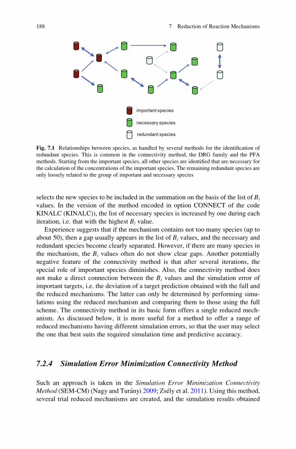
selects the new species to be included in the summation on the basis of the list of Bi

values. In the version of the method encoded in option CONNECT of the code

KINALC (KINALC)), the list of necessary species is increased by one during each

iteration, i.e. that with the highest Bi value.

Experience suggests that if the mechanism contains not too many species (up to

about 50), then a gap usually appears in the list of Bi values, and the necessary and

redundant species become clearly separated. However, if there are many species in

the mechanism, the Bi values often do not show clear gaps. Another potentially

negative feature of the connectivity method is that after several iterations, the

special role of important species diminishes. Also, the connectivity method does

not make a direct connection between the Bi values and the simulation error of

important targets, i.e. the deviation of a target prediction obtained with the full and

the reduced mechanisms. The latter can only be determined by performing simu-

lations using the reduced mechanism and comparing them to those using the full

scheme. The connectivity method in its basic form offers a single reduced mech-

anism. As discussed below, it is more useful for a method to offer a range of

reduced mechanisms having different simulation errors, so that the user may select

the one that best suits the required simulation time and predictive accuracy.

7.2.4 Simulation Error Minimization Connectivity Method

Such an approach is taken in the Simulation Error Minimization ConnectivityMethod (SEM-CM) (Nagy and Turanyi 2009; Zsely et al. 2011). Using this method,

several trial reduced mechanisms are created, and the simulation results obtained

important species

necessary species

redundant species

Fig. 7.1 Relationships between species, as handled by several methods for the identification of

redundant species. This is common in the connectivity method, the DRG family and the PFA

methods. Starting from the important species, all other species are identified that are necessary for

the calculation of the concentrations of the important species. The remaining redundant species are

only loosely related to the group of important and necessary species


guide the further search for the nearly optimal reduced mechanism. Consequently,

the application of the reduction method requires much more computer time than the

simple connectivity method but may find a much smaller reduced mechanism. The

main advantage of the method is that the required accuracy of the reduced mech-

anism (the acceptable simulation error) can be defined a priori.

The aim of the SEM-CM method is that all species within the reduced mecha-

nism be living species. A species is called a living species if its initial concentrationis nonzero, it has an influx (e.g. emission to an atmospheric chemical system) or it is

produced by chemical reactions. Vol’pert (1972) has also used the term reachablespecies for such types of species. As the definition indicates, the list of living

species is determined by not only the reaction mechanism itself but also the initial

and boundary conditions. A reaction mechanism is called consistent if all species

within it are living. A complementary set consists of those species that are not yetselected but would yield at least one additional selected reaction if these were

introduced to the current group of selected species.

The algorithm of the SEM-CM method, as detailed in the article of Nagy and

Turanyi (2009), is rather complex, and only a brief summary is given here. First, the

complementary sets of species having the strongest connection to the important

species are searched for. If necessary, the mechanisms obtained are made to be

consistent. Using these mechanisms, simulations are carried out at all investigated

conditions, and the simulation error together with the corresponding mechanism is

stored in a database. Starting from the mechanisms associated with the smallest

simulation errors, the number of species is gradually increased by adding new

complementary sets. In each step, the mechanism obtained is made consistent,

simulations are carried out and new entries are added to the database. The number

of species is increased until the simulation error decreases below a certain thresh-

old. Whilst other species reduction methods use a top-down approach, always

eliminating the species least connected to the important species, the SEM-CM

method is a bottom-up approach, and a series of consistent mechanisms are built

up using the important species as a core. An advantage of the method is that the

generated database contains a wide variety of reduced mechanisms, each belonging

to different simulation error. In this way an almost optimal reduced mechanism can

be obtained to any requested simulation error. Results obtained in a study of the

performance of the SEM-CM method compared with several other methods (CM,

DRG restart, DRGASA) are presented later in Fig. 7.5.

7.3 Identification of Redundant Reaction Steps

Using Rate-of-Production and Sensitivity Methods

So far we have discussed the removal of redundant species from a mechanism. It

may also be useful to reduce the number of reactions for the remaining necessary

species since the calculation of their rates at each time step can be computationally

7.3 Identification of Redundant Reaction Steps Using Rate-of-Production and. . . 189

time consuming. Several methods exist for reducing the number of reactions within

a mechanism. An early method for the identification of redundant reaction steps is

the use of rate-of-production analysis. Here the percentage contribution of each

reaction step to the production and consumption rate of each species is investigated

at several reaction times during a simulation. A reaction step can be eliminated

from the mechanism (at least at the simulation conditions under investigation) if the

contribution of the reaction step is less than s% to either the production or the

consumption rate of any species at any time. This threshold value is selected by the

user, and a typical value may be, for example, 5 %. The size of the reduced

mechanism (and the simulation error) can be changed by tuning this threshold.

This method is easy to understand and to apply, but not always very effective.

The simulation error depends on the selection of s, but there is no direct relationshipbetween it and the value of s. Moreover, due to the nonlinearity of chemical kinetic

systems, it is not guaranteed that the simulation error decreases when s decreases.The method would be made more effective by selecting a different threshold si foreach species. These methods can be applied for the removal of reaction steps as well

as species by basically removing those reaction steps that do not form an important

direct or indirect pathway between species which are to be retained in the

mechanism.

The method of principal component analysis of matrix S (PCAS) was discussed

in Sect. 5.3. The PCAS method allows the identification of the most important

parameters related to selected simulation results. Therefore, if the objective func-

tion includes the concentrations of the important and necessary species (see

Sect. 7.2) and the investigated parameters are the rate coefficients (or A-factors)of the reaction steps (Vajda et al. 1985; Vajda and Turanyi 1986; Turanyi 1990b;

Xu et al. 1999; Liu et al. 2005), it is also applicable for the generation of a reduced

mechanism containing less reaction steps. A further development of the PCAS

method is functional principal component analysis (fPCA) (Gokulakrishnan

et al. 2006). This method facilitates the investigation of temporal and spatial

changes in the importance of reaction steps in reaction�diffusion systems.

Another method for removing redundant reaction steps is the principal compo-nent analysis of matrix F (PCAF), where F¼ {∂fi/∂xk} (Turanyi et al. 1989;

Tomlin et al. 1992; Borger et al. 1992; Heard et al. 1998; Carslaw et al. 1999;

Zsely and Turanyi 2001; Bahlouli et al. 2014). Here the sensitivity of the net rates of

production of species to changes in the input parameters is investigated. Using the

PCAF method, the objective function has the following form:

e0 ¼

XNR

i¼1

ef i tð Þ � f i tð Þf i tð Þ

!2

ð7:2Þ

where fi and ef i are the right-hand side of the kinetic system of ODEs (2.9),

calculated at the original parameter vector α¼ ln x and at the modified values of

parameters α+Δα, respectively. This objective function can be approximated

(Turanyi et al. 1989) by


http://dx.doi.org/10.1007/978-3-662-44562-4_5#sec9

e0 αð Þ � Δαð ÞTeFTeF Δαð Þ ð7:3Þ

where eF ¼ xk=f ið Þ ∂f i=∂xkð Þf g is the normalised F-matrix and its rows correspond

to the variables present in the objective function (7.2). The elements of the matrix eFcan be calculated algebraically from the concentration vector and therefore

obtained from a single simulation, whilst even the most effective calculation of

the sensitivity matrix eS requires significantly more computer time (see Sect. 5.2). If

fi is the right-hand side of the kinetic system of ODEs for species i (2.9) and

parameter kj is the rate coefficient of the reaction step j, then the elements of matrixeF can be easily calculated (Turanyi et al. 1989) as

eFi, j ¼ ∂ln f i∂lnkj

¼ kjf i

∂f i∂kj

¼ νijrjf i

� �ð7:4Þ

If temperature is also considered in the objective function, then the enthalpies of

formation of the species and heat capacity of the reaction mixture also have to be

taken into account (Zsely and Turanyi 2003).

The eigenvalues of matrix eFTeF indicate the effectiveness of a simultaneous

change of the values of a group of parameters on the production rates of species.

Elements of the eigenvectors show the weight of the individual parameters in the

corresponding parameter group. In common with the PCAS method, the PCAF

method can determine a list of important reactions, if the parameters investigated

are the rate coefficients (or A-factors) of the reaction steps, and the objective

function includes the production rates of the important and necessary species.

Although the PCAS and PCAF methods are similar in form, these two methods

are fundamentally different. The objective function of PCAF contains the produc-

tion rates of species, and the matrix F can be calculated from the right-hand side of

ODE (2.9). The objective function of PCAS contains the concentrations of species

[the solution of ODE (2.9)], and the matrix S has to be obtained from the solution of

the sensitivity differential equations (5.7) and is therefore computationally more

time consuming. Put another way, PCAS investigates the effect of parameter

changes on the solution of the kinetic system of ODEs, whilst PCAF examines

the effect of parameter changes on the right-hand sides of the kinetic system of

ODEs (2.9).

When the importance of reactions is investigated using PCAF over an interval of

time or distance, the analysis has to be carried out at several independent variable

sets. This means that the change in importance of reaction steps over time

(or distance) can be monitored with arbitrary resolution. If two different models

(e.g. an ignition and a flame model) provide identical concentration and tempera-

ture profiles using the same reaction mechanism, then PCAF will provide identical

importance measures for the reaction steps (Zsely and Turanyi 2003). On the other

hand, PCAS investigates the local sensitivity matrices, which indicate the effect of

a parameter perturbation on the time-dependent solution, so that very different

7.3 Identification of Redundant Reaction Steps Using Rate-of-Production and. . . 191

http://dx.doi.org/10.1007/978-3-662-44562-4_5#sec2

sensitivity functions may belong to the same reaction mechanism and concentra-

tion—time functions. Moreover, PCAS investigates the integrated deviations in

solution (see Eq. 5.15), and therefore, the reaction importance belongs to an interval

of time. Another consequence of the differences is that using PCAF, it may be

important to apply the analysis over many time or distance points along reaction

trajectories in order to ensure that reactions which are only of importance over a

subset of the whole domain are picked up by the analysis. Often a simple model

scenario can be used (e.g. zero-dimensional reactor simulations or a 1D flame

simulation) for the reduction process, and, as long as the concentration, temperature

and pressure profiles match those of the final practical model, the reduced models

generated can be of use in larger modelling scenarios such as 3D simulations. The

use of adaptive reduction where different reduced schemes are utilised over differ-

ent subsets of the domain is discussed below.

7.4 Identification of Redundant Reaction Steps Based

on Entropy Production

All of the previous methods identify redundant reactions via the inspection of the

reaction rates or by the study of sensitivity matrices deduced from the kinetic

system of differential equations. A very different approach is the application of

thermodynamic functions for the identification of redundant reactions. This

approach has common features with the derivation of numerical reduced models

based on thermodynamics reasoning (see Sect. 7.10.4).

Kooshkbaghi et al. (2014) published a systematic approach based on the relative

contribution of each elementary reaction to the total entropy production. In a closed

system, the total entropy production per unit volume is a positive semidefinite

function that can be calculated in the following way:

dS

dt¼ R

XNRj¼1

rf, j � rb, j� �

lnrf, jrb, j

� �ð7:5Þ

The entropy production vanishes at equilibrium. The relative contribution of each

reaction step to the total entropy production is given by

qj ¼ RXNRj¼1

rf , j � rb, j� �

lnrf , jrb, j

� �" #dS

dt

� �1

ð7:6Þ

Here R is the gas constant and rf,j and rb,j are the rates of the j-th forward and

backward reaction steps, respectively. Kooshkbaghi et al. (2014) investigated the

effect of eliminating all reaction steps having qj relative entropy production less

than a threshold ε for an example of an n-heptane ignition mechanism. Their


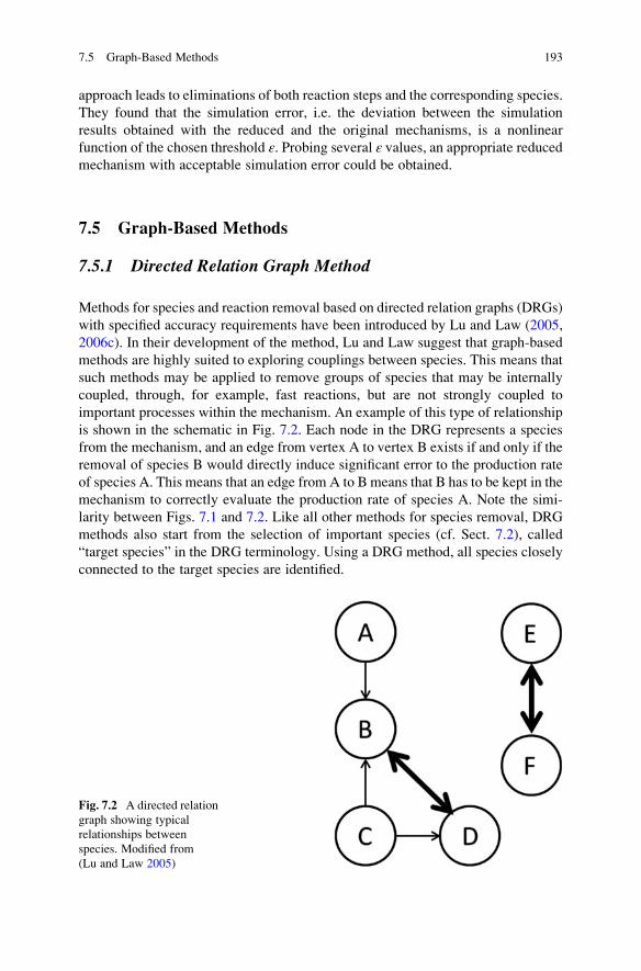
approach leads to eliminations of both reaction steps and the corresponding species.

They found that the simulation error, i.e. the deviation between the simulation

results obtained with the reduced and the original mechanisms, is a nonlinear

function of the chosen threshold ε. Probing several ε values, an appropriate reducedmechanism with acceptable simulation error could be obtained.

7.5 Graph-Based Methods

7.5.1 Directed Relation Graph Method

Methods for species and reaction removal based on directed relation graphs (DRGs)

with specified accuracy requirements have been introduced by Lu and Law (2005,

2006c). In their development of the method, Lu and Law suggest that graph-based

methods are highly suited to exploring couplings between species. This means that

such methods may be applied to remove groups of species that may be internally

coupled, through, for example, fast reactions, but are not strongly coupled to

important processes within the mechanism. An example of this type of relationship

is shown in the schematic in Fig. 7.2. Each node in the DRG represents a species

from the mechanism, and an edge from vertex A to vertex B exists if and only if the

removal of species B would directly induce significant error to the production rate

of species A. This means that an edge from A to B means that B has to be kept in the

mechanism to correctly evaluate the production rate of species A. Note the simi-

larity between Figs. 7.1 and 7.2. Like all other methods for species removal, DRG

methods also start from the selection of important species (cf. Sect. 7.2), called

“target species” in the DRG terminology. Using a DRG method, all species closely

connected to the target species are identified.

Fig. 7.2 A directed relation

graph showing typical

relationships between

species. Modified from

(Lu and Law 2005)

7.5 Graph-Based Methods 193

The various DRG-based reduction methods all state a connection weight

between pairs of species. These weights define the directed relation graph structure.

Starting from the target species, an importance coefficient is calculated for all other

species, which quantifies how strongly a given species is connected to the target

species. Then, all species are eliminated from the mechanism (with their reactions)

whose importance coefficient is below a user-defined threshold. The DRG-based

methods differ in their definitions of connection weights and importance coeffi-

cients. Tosatto et al. (2013) compared the various DRG-based methods, and we

follow their notations in the discussion below.

The original DRG method of Lu and Law (2005) defines the connection weight

from species i to species j in the following way:

RLuð Þi!j ¼

Xα2C i;jð Þ νiαrαj jXα2R ið Þ νiαrαj j ð7:7Þ

where R(i) is the set of reactions that are related to species i, C(i, j) is the set of

reactions in which both species i and j participate, νiα is the stoichiometric coeffi-

cient of species i in reaction α and rα is the net reaction rate (the difference of the

forward and backward rates).

A variant of the DGR method was suggested by Luo et al. (2010a) for the

reduction of reaction mechanisms containing many isomers. Luo

et al. recommended the application of the maximum norm instead of the

summation:

RLuoð Þi!j ¼ maxα2C i;jð Þ νiαrαj j

maxα2R ið Þ νiαrαj j ð7:8Þ

The original DRG method of Lu and Law (2005) defines the importance

coefficient of species i as

IDRGð Þi ¼ 1 if species i is a target species

maxj2S

min Rj!i;IDRGð Þjð Þð Þ otherwise

(ð7:9Þ

Here S is the full set of chemical species and Rj! i is a connection weight defined in

Eqs. 7.7 and 7.8, and it is implicitly assumed that if two species are not connected,

then Rj! i¼ 0. This approach defines the importance coefficient for species i as thesmallest connection on any path towards a target species. Ii

(DRG) is calculated

iteratively using a minimum-cost graph search algorithm (Lu and Law 2005). A

small threshold value ε can be defined, and if IðDRGÞi < ε, then species i is consideredto be redundant for the simulation of the target species. Hence, in Fig. 7.2, if A is an

important species, then D must be retained within the scheme since although it is

not directly coupled to A, it is part of the dependent set of A by being directly

coupled to B, where B is coupled to A. In this example species E and F are


interconnected by a pair of fast reversible reactions, since, although they are

strongly coupled to each other, they do not couple to any species in the dependent

set of A. The strong two-way coupling between these species indicates that they

should be removed as a pair.

In common with the connectivity method (CM, Sect. 7.2.3), the DRG method

requires a set of important species (“target species”) to be specified which may

include the main reactants and important products of the starting reaction mecha-

nism. The method then seeks the dependent sets for each important species, and the

skeleton mechanism is formed from the union of these sets. The DRG method is

local in the sense that the reaction rates used are specific to a particular set of

concentrations and temperature. In common with the CM, the graph has to be

computed over a range of conditions relevant to the intended final application. For a

generally applicable reduced scheme, the final model must represent the union of

mechanisms derived for each operating condition. The success of the final reduced

scheme will depend on the relevance of the local conditions chosen for analysis and

the selected value of ε. The size of the skeleton mechanism will reduce as larger and

larger values of ε are chosen. Several thresholds can be applied and the accuracy ofthe resulting mechanisms are tested in order to select an appropriate level of

reduction. Lu and Law (2005) state that jumps in the number of required species

may occur quite abruptly, signifying groups with strong internal coupling but weak

intergroup couplings moving out of the skeleton scheme. This is analogous to the

large gaps in Bi values that occur in the Jacobian analysis and in a similar manner

can help with the selection of threshold values for ε. It should be pointed out that inboth the simple connectivity and DRG-based methods, the thresholds only control

the local accuracy of the rates of production of necessary species, which does not

automatically control the potential growth of errors in a time or spatially dependent

model. The impact of local errors could be determined via more expensive methods

or simulations compared to the full model.

Figure 7.3 shows the result of an investigation where the DRG threshold ε waschanged systematically for an example of the reduction of a methane partial

oxidation mechanism (Nagy and Turanyi 2009). The number of species remaining

within the reduced mechanism decreased almost linearly on increasing the loga-

rithm of ε. The most interesting result was that the simulation error did not change

monotonically with increasing ε. Also, sudden jumps indicated that sometimes

using only a slightly higher ε gave a much worse reduced mechanism, as explained

above.

The DRG method was first applied to a model system of ethylene combustion

(Lu and Law 2005; Luo et al. 2011) with a full scheme of 70 species. A value of ε of0.16 gave a skeleton scheme of 33 species, i.e. quite a substantial degree of

reduction. In application to n-heptane and iso-octane combustion using full

schemes of 561 and 857 species (Lu and Law 2006c), ε values of 0.19 and 0.17

resulted in reduced schemes of 188 and 233 species, respectively. DRG methods

have since been widely applied for the reduction of large combustion schemes

including for methane (Sankaran et al. 2007), primary reference fuel (Lu and Law


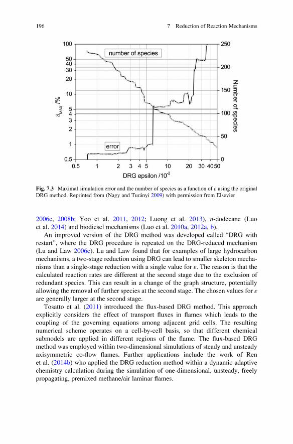
2006c, 2008b; Yoo et al. 2011, 2012; Luong et al. 2013), n-dodecane (Luo

et al. 2014) and biodiesel mechanisms (Luo et al. 2010a, 2012a, b).

An improved version of the DRG method was developed called “DRG with

restart”, where the DRG procedure is repeated on the DRG-reduced mechanism

(Lu and Law 2006c). Lu and Law found that for examples of large hydrocarbon

mechanisms, a two-stage reduction using DRG can lead to smaller skeleton mecha-

nisms than a single-stage reduction with a single value for ε. The reason is that the

calculated reaction rates are different at the second stage due to the exclusion of

redundant species. This can result in a change of the graph structure, potentially

allowing the removal of further species at the second stage. The chosen values for εare generally larger at the second stage.

Tosatto et al. (2011) introduced the flux-based DRG method. This approach

explicitly considers the effect of transport fluxes in flames which leads to the

coupling of the governing equations among adjacent grid cells. The resulting

numerical scheme operates on a cell-by-cell basis, so that different chemical

submodels are applied in different regions of the flame. The flux-based DRG

method was employed within two-dimensional simulations of steady and unsteady

axisymmetric co-flow flames. Further applications include the work of Ren

et al. (2014b) who applied the DRG reduction method within a dynamic adaptive

chemistry calculation during the simulation of one-dimensional, unsteady, freely

propagating, premixed methane/air laminar flames.

Fig. 7.3 Maximal simulation error and the number of species as a function of ε using the originalDRG method. Reprinted from (Nagy and Turanyi 2009) with permission from Elsevier


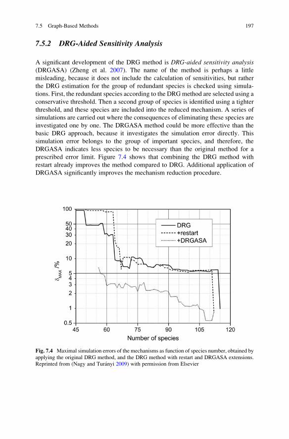
7.5.2 DRG-Aided Sensitivity Analysis

A significant development of the DRG method is DRG-aided sensitivity analysis(DRGASA) (Zheng et al. 2007). The name of the method is perhaps a little

misleading, because it does not include the calculation of sensitivities, but rather

the DRG estimation for the group of redundant species is checked using simula-

tions. First, the redundant species according to the DRGmethod are selected using a

conservative threshold. Then a second group of species is identified using a tighter

threshold, and these species are included into the reduced mechanism. A series of

simulations are carried out where the consequences of eliminating these species are

investigated one by one. The DRGASA method could be more effective than the

basic DRG approach, because it investigates the simulation error directly. This

simulation error belongs to the group of important species, and therefore, the

DRGASA indicates less species to be necessary than the original method for a

prescribed error limit. Figure 7.4 shows that combining the DRG method with

restart already improves the method compared to DRG. Additional application of

DRGASA significantly improves the mechanism reduction procedure.

Fig. 7.4 Maximal simulation errors of the mechanisms as function of species number, obtained by

applying the original DRG method, and the DRG method with restart and DRGASA extensions.

Reprinted from (Nagy and Turanyi 2009) with permission from Elsevier


7.5.3 DRG with Error Propagation

Pepiot-Desjardins and Pitsch (2005, 2008) noticed that Eq. (7.7) does not distin-

guish between reactions that create or destroy species i and suggested an alternativedefinition:

RPepð Þi!j ¼

Xα2C i;jð Þνiαrα

max

Xα2R ið Þ νiαrαð Þþ;

Xα2R ið Þ νiαrαð Þ�

� � ð7:10Þ

The operator (.)+ selects only the positive terms in the summation, and the operator

(.)� selects only the negative terms and makes them positive. Equation (7.10)

calculates the ratio of the sum of the rates belonging to the pair of species (i, j) tothe total rate of formation or destruction of species i. Note that all forward and

backward rates must be considered separately as a single reaction when using the

connection weights (7.10), or else partial equilibrium reactions could result in

artificially low connection weights.

Pepiot-Desjardins and Pitsch (2008) made further extensions to DRG by incorpo-

rating error propagation, called DRG with error propagation (DRGEP). In this

method the assumption that all coupled species are equally important in the mecha-

nism is lost, and errors are damped as they propagate along the graph from the

initially selected important species. The importance index is therefore calculated as

IDRGEPð Þi ¼

1 if species i is a target species

maxj2S

Rj!i � I DRGEPð Þj

� �otherwise

(ð7:11Þ

The aim of error propagation is to try to eliminate more species using the same

threshold error by better estimating the induced error, rather than using its upper

bound. The approach is combined with an integrity check which aims to avoid

truncated chemical paths that may lead to mass accumulation in intermediate

species whose consumption paths have been removed. However, for chains of

propagating reactions with several fast steps, this may lead to an underestimation

of errors since in this case the fast species can be related to the slow ones through

algebraic expressions (see Chap. 6) leading to a single rate-determining step within

the sequence. According to Lu and Law (2006c), the error propagation method in

such cases should be linked to an investigation of the slow and fast subspaces.

The DRGEP approach has been applied adaptively in order to produce on-the-flyreduced mechanisms for n-heptane (Shi et al. 2010b) and gasoline surrogate mixtures

(Liang et al. 2009b; Shi et al. 2010a) in simulations of homogeneous charge com-

pression ignition. In Liang et al. (2009b), computational speed-ups of a factor of

70 were achieved when compared to a detailed starting mechanism containing 1,099

species. The number of species required in the locally reduced models varies

throughout the calculations but reaches a maximum of about one third of the number

of initial species. The DRG and DRGEP methods were compared for an example of


http://dx.doi.org/10.1007/978-3-662-44562-4_6

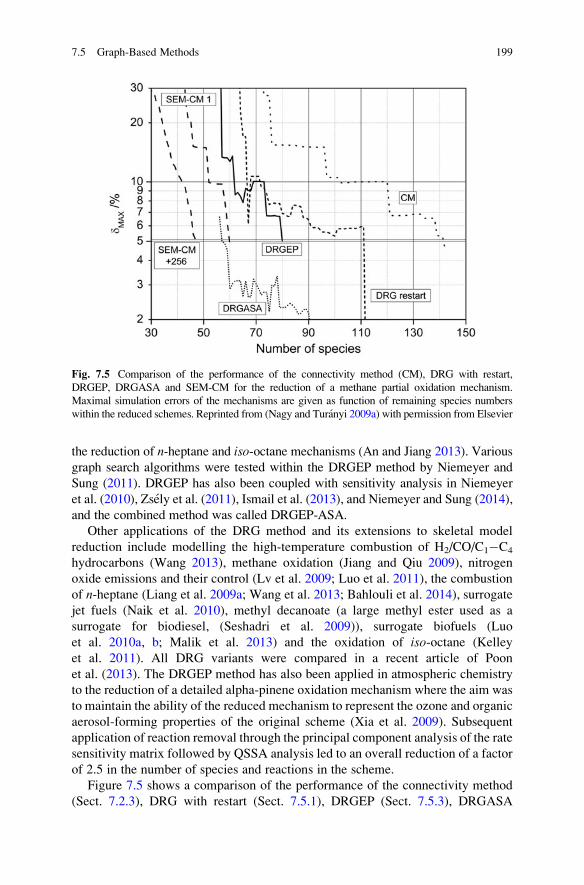
the reduction of n-heptane and iso-octane mechanisms (An and Jiang 2013). Various

graph search algorithms were tested within the DRGEP method by Niemeyer and

Sung (2011). DRGEP has also been coupled with sensitivity analysis in Niemeyer

et al. (2010), Zsely et al. (2011), Ismail et al. (2013), and Niemeyer and Sung (2014),

and the combined method was called DRGEP-ASA.

Other applications of the DRG method and its extensions to skeletal model

reduction include modelling the high-temperature combustion of H2/CO/C1�C4

hydrocarbons (Wang 2013), methane oxidation (Jiang and Qiu 2009), nitrogen

oxide emissions and their control (Lv et al. 2009; Luo et al. 2011), the combustion

of n-heptane (Liang et al. 2009a; Wang et al. 2013; Bahlouli et al. 2014), surrogate

jet fuels (Naik et al. 2010), methyl decanoate (a large methyl ester used as a

surrogate for biodiesel, (Seshadri et al. 2009)), surrogate biofuels (Luo

et al. 2010a, b; Malik et al. 2013) and the oxidation of iso-octane (Kelley

et al. 2011). All DRG variants were compared in a recent article of Poon

et al. (2013). The DRGEP method has also been applied in atmospheric chemistry

to the reduction of a detailed alpha-pinene oxidation mechanism where the aim was

to maintain the ability of the reduced mechanism to represent the ozone and organic

aerosol-forming properties of the original scheme (Xia et al. 2009). Subsequent

application of reaction removal through the principal component analysis of the rate

sensitivity matrix followed by QSSA analysis led to an overall reduction of a factor

of 2.5 in the number of species and reactions in the scheme.

Figure 7.5 shows a comparison of the performance of the connectivity method

(Sect. 7.2.3), DRG with restart (Sect. 7.5.1), DRGEP (Sect. 7.5.3), DRGASA

Fig. 7.5 Comparison of the performance of the connectivity method (CM), DRG with restart,

DRGEP, DRGASA and SEM-CM for the reduction of a methane partial oxidation mechanism.

Maximal simulation errors of the mechanisms are given as function of remaining species numbers

within the reduced schemes. Reprinted from (Nagy and Turanyi 2009a) with permission from Elsevier


(Sect. 7.5.2) and SEM-CM (Sect. 7.2.4) for the reduction of a methane partial

oxidation mechanism (Nagy and Turanyi 2009). Method SEM-CM is presented in

two versions, one is faster and less effective (“1”), and the other is slower and more

effective (“256”). For each method, the most effective version was used in the

comparison. In general, a mechanism reduction method is more effective if the

simulation error is smaller for the same number of species or if the same simulation

error can be achieved with a mechanism having less species. For this example, the

SEM-CM method proved to be the most effective; however, we have to keep in

mind that the application of this method requires much more computer time

compared to the other methods.

7.5.4 The Path Flux Analysis Method

Path flux analysis (PFA) is a method, similar to DRG, for the generation of skeletal

mechanisms (Sun et al. 2010; Gou et al. 2013). In the PFA method, the production

and consumption fluxes are used to identify the important reaction pathways. The

first-generation production (PA) and consumption (CA) fluxes of species A are

calculated according to equations

PA ¼Xi

max νA, iωi, 0ð Þ ð7:12Þ

CA ¼Xi

max �νA, iωi, 0ð Þ ð7:13Þ

where νA,i is the stoichiometric coefficient of species A in the i-th reaction and ωi is

the net reaction rate of this reaction. The production (PAB) and consumption (CAB)

fluxes of species A via species B are calculated by

PAB ¼Xi

max νA, iωi δiB, 0

� � ð7:14Þ

CAB ¼Xi

max �νA, iωi δiB, 0

� � ð7:15Þ

where δiB is unity if species B is involved in the i-th reaction and 0 otherwise. A flux

ratio is introduced to represent the share of a particular production and consumption

path via species B to the total production and consumption flux of species A. The

first-generation flux ratios for the production and consumption of species A via

species B are defined as


rpro�1stAB ¼ PAB

max PA;CAð Þ ð7:16Þ

rcon�1stAB ¼ CAB

max PA;CAð Þ ð7:17Þ

At each time step, production and consumption flux ratios rpro� 1stAB and rcon� 1st

AB are

calculated. This process only involves the calculation of the reaction rates, and the

CPU time is linearly proportional to the number of species. The reduction starts

from the important species and then identifies whether to retain species B in the

reduced model by evaluating if the flux ratios of species A via species B satisfy the

relation rAB> ε, where ε is a threshold value and rAB¼max(rpro� 1stAB , rcon� 1st

AB ).

An iterative process is used to find the path fluxes of each selected species.

Starting from the set of important species, using the relation rAB> ε, the set of othernecessary species are identified. These are added to the investigated set, and the

iterative process is continued until no new necessary species are found. Gou

et al. (2013) used the PFA method to create a dynamic adaptive chemistry scheme

for n-heptane and n-decane combustion mechanisms.

7.5.5 Comparison of Methods for Species Elimination

A common feature of the connectivity, PFA, DRG and DRGEP methods (with or

without ASA) is that the list of important species has to be defined. Then, points on

the concentration trajectory are selected, and the analysis is carried out at these

points. The set of necessary species are determined at each of the chosen points, and

the reaction mechanism that is applicable across the whole domain should contain

the union of the species necessary at each point unless adaptive reduction is

employed (see later discussion). The list of necessary species is determined by a

threshold (the threshold Bi value in the connectivity method and parameter ε in the

DRG, DRGEP and PFA methods), which are not linearly related to the simulation

error of the resulting reduced mechanism. In general, a smaller threshold leads to a

larger mechanism with smaller simulation error, but the decrease of the simulation

error is not necessarily monotonic. Using these methods, the efficiency of mecha-

nism reduction has to be judged a posterior: a reduction method being more

efficient if the reduced mechanism contains less species at the same level of

simulation error. We saw that extensions to these methods such as the SEM-CM,

DRGASA and DRGEP-ASA methods include the simulation error as part of the

necessary species selection and can lead to more effective reduction strategies at the

expense of computational cost. Other approaches have also been developed based

on methods from optimisation, and these will be discussed in the next section.


7.6 Optimisation Approaches

Although sensitivity analysis, DRG and CSP are perhaps the most common

methods for deriving skeletal mechanisms, the application of optimisation methods

such as linear and nonlinear integer programming is increasing for reduction

analysis. One advantage of such methods is that they preserve the nonlinearity of

the reaction system, as opposed to sensitivity analysis, which is in general based on

first-order sensitivity coefficients. These methods are based on solving an optimi-

sation problem, i.e. minimising an objective function subject to a set of constraints.

In mechanism reduction applications, the objective function is related to the model

error between the full and reduced models, which varies between applications, but

is usually based on errors in either rates of production of species or species

concentrations.

7.6.1 Integer Programming Methods

An early application of this type of approach for reaction removal was carried out

by Petzold and Zhu (1999) for several ignition problems. Although this method has

its drawbacks, we discuss it in some detail here since it provides a useful illustration

of how optimisation approaches are applied in practice. The rate of change of

species mass fractions yi is given by

_yi ¼ f yð Þ ¼XNj¼1

υijRj yð Þ ð7:18Þ

which in matrix form can be written as

_y ¼ υR yð Þ ð7:19Þ

where υ is a matrix whose columns are the stoichiometric vectors and R is the

vector of nonlinear reaction terms. A similar equation set for the reduced model can

then be described as

_z ¼ υDR zð Þ ð7:20Þ

where D is an N�N diagonal matrix whose diagonal elements dj are either 1 or

0 depending on whether the reaction j is retained in the mechanism or not. Finding

the reduced mechanism can then be expressed as a constrained optimisation

(Petzold and Zhu 1999):


min y�zk ksubject to

_y ¼ υR yð Þ, y 0ð Þ ¼ yo_z ¼ υDR zð Þ, z 0ð Þ ¼ zo 0 � t � bXNj¼1

dj ¼ k, dj ¼ 0 or 1

ð7:21Þ

where the minimum is over d1, . . ., dN and k<N. Here k is the number of reactions

in the reduced scheme and is chosen by the user. The norm is weighted according to

user supplied relative and absolute tolerances. If one was interested in the overall

error during a simulation time, then the local term min ||y� z|| could be extended to

an integral between initial time ti and final time tf, thus calculating

min

ðtfti

y tð Þ � z tð Þ�� . The resulting optimisation becomes an integer nonlinear

programming problem as discussed by Edwards et al. (2000). It is also a combi-

natorial problem. For example, for a 5-reaction starting mechanism, there are 25–1

possible reduced mechanisms. Since the number of possible reduced mechanisms

grows exponentially with reaction size, there is clearly a need to restrict the

optimisation problem where possible. Several variations on the methodology

were proposed by Petzold and Zhu to reduce the computational cost of the method.

The first is based on the fact that it may not be necessary to find the absolute

minimum of ky� zk, and any reduced mechanism with a small enough value may

be good enough. A modified version of Eq. (7.21) is proposed as

min y� zk ksubject to

_y ¼ υR yð Þ, y 0ð Þ ¼ yo_z ¼ υDR zð Þ, z 0ð Þ ¼ zo 0 � t � b

k1 �XNj¼1

dj � k2, 0 � dj � 1

g d1, . . . , dNð Þ � r

ð7:22Þ

where k1 and k2 are upper and lower bounds, respectively, on the number of

reactions in the reduced model, g is a nonlinear function which when equal to

0 forces the dj to take integer values and r is a small positive number that relaxes to

the nonlinear constraint. The restrictions on the possible number of reactions in the

reduced mechanism lower the overall number of combinations within the optimi-

sation. Petzold and Zhu use the following function to describe g:

g ¼XNj¼1

dj � dj2

� �2 ¼ 0 ð7:23Þ

The optimisation problem described by (7.22) is then solved using sequential

quadratic programming, and in order to obtain the reduced model, the values of djare rounded to 0 or 1.

7.6 Optimisation Approaches 203

The method can also be applied to the removal of species, and a two-tier

approach is suggested by Petzold and Zhu (1999) and by Mitsos et al. (2008),

where the search for redundant species is performed prior to reaction removal in

common with several other skeletal reduction approaches as outlined above. Since

the number of species is usually much lower than the number of reactions, a

significant cost saving in the application of the method can be made since all

reactions of redundant species are removed at the first stage, thus reducing the

cost of the reaction removal procedure. In addition, the method proposed by Petzold

and Zhu first applies the so-called “greedy” algorithm for both species and reaction

removal prior to the solution of the full optimisation problem. In the greedy method,

the reactions are removed from the model one by one with those causing the

smallest error under the given norm being dropped first (a trial-and-error approach

as discussed in Sect. 7.2.2). The approach scales as N2, however, which makes it

computationally costly for large reaction mechanisms. In addition, care must be

taken for mechanisms containing fast reversible reactions since, as indicated in

Sects. 7.2 and 7.5, sometimes reactions/species can be more successfully removed

in groups rather than individually.

A slightly different approach to the use of optimisation methods is presented by

Androulakis (2000) based on the minimisation of the number of reactions in the

reduced mechanism subject to constraints on the error of the reduced mechanism

with respect to the full scheme. In this example, a weighted error norm containing

terms involving species mass fractions, temperature and induction time for the

reaction is developed. In common with the approach of Petzold and Zhu (1999), a

pre-processing step is applied in this work to identify a subset of important

reactions with high ranking based on removing the reactions one at a time. This

subset is then excluded from the constraints in the full optimisation problem in

order to improve computational efficiency. Problems with fast reversible reactions

may also be encountered using this approach, and hence, the use of this

pre-processing step will lead to an upper bound on the numbers of reactions within

the final reduced scheme. The application of species removal prior to reaction

removal may help to alleviate this problem.

The integer programming technique applied by Androulakis is a branch-and-

bound algorithm which splits the feasible region of input values into smaller sub-

regions (branching) with the subregions forming a search tree. Upper and lower

bounds on the optimal solution in each subregion can then be determined

(bounding), and if the lower bound for a subregion A from the search tree is greater

than the upper bound for any other (previously examined) subregion, then Amay be

safely discarded from the search (pruning). If an optimal solution is found to a

subregion (e.g. if the upper bound matches the lower bound), it is a feasible solution

to the full problem, but not necessarily globally optimal. It can be used for pruning,

however, since if the lower bound for a node exceeds the best known feasible

solution, no globally optimal solution can exist in the subspace of the feasible

region represented by the node. The procedure stops when all nodes of the search

tree are either pruned or solved. Within the subregions, the relaxation of the integer

problem is solved by successive quadratic programming. The methods are


illustrated for a hydrogen combustion model in a stirred reactor where the use of

different objective functions is compared. Androulakis shows that the use of errors

at only the final time point leads to a smaller reaction mechanism when compared to

using a range of reaction times, but does not give a good representation of the

intermediate dynamics. The approach was also applied to species removal by

Androulakis (2000) and Banerjee and Ierapetritou (2003).

Anderson et al. (2011) transformed the original chemical kinetic model of a

mitogen-activated protein kinase (MAPK) signalling pathway to a linear

parameter-varying (LPV) model. This LPV model was then used to identify loosely

connected blocks of the original model, taking into account the uncertainty ranges

of the important parameters. Hannemann-Tamas et al. (2014) considered mecha-

nism reduction as a convex mixed-integer quadratic problem, for which efficient

solvers exist. They discussed the relationship of this approach with the sensitivity

analysis-based mechanism reduction methods (Sect. 7.3). The rate coefficients of

the reduced mechanisms were optimised to give a better reproduction of solutions

of the full mechanisms.

One advantage of integer programming methods is that they can be formulated

in a general way, and the constraints can therefore include any required measure of

the simulation error between the reduced and full models. This means that the

actual simulation error in important species or target outputs can be taken into

account, in contrast to the standard DRG and connectivity methods discussed above

which were based on local approaches. However, for large mechanisms, the number

of possible reduced mechanisms could be huge, and if each were to be tested, then

the methods become very computationally costly. Screening type algorithms have

therefore been included using the so-called greedy approach, but these are really

trial-and-error-based algorithms, and as discussed in Sect. 7.2.1, they ignore the

couplings between species. In order to make reduction algorithms more efficient, it

is sensible to utilise the information on species couplings contained either in the

Jacobian matrix or the DRG, and hence, the combination of the connectivity

approach with error minimisation as used in the Simulation Error Minimization

Connectivity Method (SEM-CM, Sect. 7.2.4) is likely to be more computationally

effective.

A further extension of integer programming methods was also developed in the

work of Bhattacharjee et al. (2003) based on earlier ideas developed in Schwer

et al. (2003). Here the reduction is based on a linear integer programming method

providing computational savings over nonlinear methods. The linearity is achieved

by applying constraints to local rates of production rather than to concentration and

temperature profiles, forcing the error constraints to be linear in the rates of

production. Therefore, similarly to the results of reduction methods based on

DRG or rate sensitivity matrices, the reduced mechanisms are only strictly appli-

cable for the local points at which they were generated. The global error is now also

related to the locally controlled error in a more complex way, since small local

errors in rates of production may grow and propagate during time-dependent

simulations. The derivation of a rigorous quantitative relationship between the


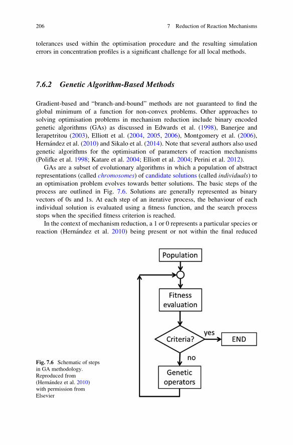
tolerances used within the optimisation procedure and the resulting simulation

errors in concentration profiles is a significant challenge for all local methods.

7.6.2 Genetic Algorithm-Based Methods

Gradient-based and “branch-and-bound” methods are not guaranteed to find the

global minimum of a function for non-convex problems. Other approaches to

solving optimisation problems in mechanism reduction include binary encoded

genetic algorithms (GAs) as discussed in Edwards et al. (1998), Banerjee and

Ierapetritou (2003), Elliott et al. (2004, 2005, 2006), Montgomery et al. (2006),

Hernandez et al. (2010) and Sikalo et al. (2014). Note that several authors also used

genetic algorithms for the optimisation of parameters of reaction mechanisms

(Polifke et al. 1998; Katare et al. 2004; Elliott et al. 2004; Perini et al. 2012).

GAs are a subset of evolutionary algorithms in which a population of abstract

representations (called chromosomes) of candidate solutions (called individuals) toan optimisation problem evolves towards better solutions. The basic steps of the

process are outlined in Fig. 7.6. Solutions are generally represented as binary

vectors of 0s and 1s. At each step of an iterative process, the behaviour of each

individual solution is evaluated using a fitness function, and the search process

stops when the specified fitness criterion is reached.

In the context of mechanism reduction, a 1 or 0 represents a particular species or

reaction (Hernandez et al. 2010) being present or not within the final reduced

Fig. 7.6 Schematic of steps

in GA methodology.

Reproduced from

(Hernandez et al. 2010)

with permission from

Elsevier


http://en.wikipedia.org/wiki/Chromosome_%28genetic_algorithm%29#Chromosome%20(genetic%20algorithm)

http://en.wikipedia.org/wiki/Candidate_solutions#Candidate%20solutions

model. For example, an initial population of four individuals for a final reduced

model specified to have five species from a full model with ten species may be

written as follows:

Individual 1 1100101010




Important species may also be defined such as fuel, oxidiser or important

products. Species 1 and 2 in the above example are always fixed at 1, i.e. always

present in the mechanism, thus reducing the search space by 2. A reaction is chosen

to be present in the reduced model only if all reactant and product species exist

within the reduced species set. The fitness criterion is then used to determine which

individuals to propagate to the next generation. For example, Elliot et al. (2005) use

a criterion based on a weighted sum of errors in species molar concentrations using

an L2 norm. The fittest individuals are then selected probabilistically using a k-tournament selection in order to be parents for the next generation. Cross-over and

mutation (genetic operators) are then used to exchange information between parents

in order to develop the next generation of individuals as described in Harris

et al. (2000). The approach involves selecting two parents and identifying those

species common to both parents. A child is formed by keeping common species and

randomly selecting new ones from unused positions in the chromosome. Mutation

is used to avoid local minima. The fitness criterion is then used again, and the fittest

parents and children are selected to form a new generation. After a certain number

of generations, where there is no further improvement, the best chromosome

represents an optimal solution. The method was successfully applied in Elliott

et al. (2005) to the reduction of the GRI methane oxidation mechanism to a

16-species skeleton mechanism, although even when using a fairly large set of

important species, the optimisation process took 2 days of CPU on a 3.2 GHz

Pentium 4 processor. The method was further extended to optimisation of the rate

parameters in the reduced scheme based on an experimental set of 1D laminar flame

profiles. The combined approach of model reduction and parameter selection using

GA-based optimisation methods has also been applied to biochemical networks in

Mauryaa et al. (2006, 2009) and to reduced models for the combustion of aviation

fuels in Elliott et al. (2006).

A slightly different approach was applied in the earlier work of Edwards

et al. (1998) where the search was for the minimum number of reactions/species

needed to satisfy specified error bounds rather than for the best reduced mechanism

for a fixed number of species and a given error tolerance. A heuristic comparison

was made in this work between the computational expense of the GA approach and

global sensitivity-based methods. The number of functional evaluations for the GA

approach was stated to be lower than for global sensitivity analysis, although the

same would not be true for the local rate sensitivity and DRG-based methods

described above. The potential user therefore has the choice between applying

global methods such as optimisation with the associated computational expense


of acquiring a truly global solution or the use of much more computationally

efficient local methods, with the proviso that they are highly dependent on the

conditions chosen for analysis and the nominal values of the rate parameters. The

application of these types of methods is to a certain extent user driven. The user

may wish to specify a tolerated error in the prediction of a target output. On the

other hand, it may also be useful to use such methods to identify the optimal scheme

for a given number of variables. For example, in complex flow models such as

3-dimensional turbulence problems, a limited number of scalars can usually be

tolerated within the code due to computational costs. In such cases it may be better

to define the allowed number of variables and to use an optimisation approach.

Sikalo et al. (2014) compared several options for the application of genetic

algorithms to mechanism reduction, exploring the trade-off between the size and

accuracy of the resulting mechanisms. Information on the speed of solution was

also taken into account, so that, for example, the least stiff system (Sect. 6.7) could

be selected. An automatic method for the reduction of chemical kinetic mechanisms

was suggested and tested for the performance of reduced mechanisms used within

homogeneous constant pressure reactor and burner-stabilised flame simulations.

The flexibility of this type of approach has clear utility when restrictions are placed

on the number of variables that can be tolerated within a scheme in the compu-

tational sense. However, the development of skeletal mechanisms is rarely the end

point of any reduction procedure since the application of lumping or timescale-

based methods can be applied subsequently. These methods will be discussed in

later sections.

7.6.3 Optimisation of Reduced Models to Experimental Data

Usually, the aim of a reduction algorithm is to produce a skeletal scheme with

minimal error compared to the full scheme over a wide range of conditions.

However, if a large degree of reduction is required, e.g. for use in a spatially 3D

calculation, then simulation errors may creep in. In some circumstances it may

therefore be necessary to make adjustments to the model within the bounds of

uncertainty of its parameters, in order to improve agreement with target experi-

mental data. Apri et al. (2012, 2014) developed such an approach based on

optimisation, where mechanism reduction and parameter estimation were coupled

via comparison to experimental data. In their method they optimise the full model

to experimental data and then try to remove species and reactions from the model,

in order of increasing normalised local sensitivity coefficients. The trial reduced

model is re-optimised to the experimental data, and the mechanism reduction is

considered successful, if the given set of experimental data cannot discriminate

between the full and the reduced mechanisms. If the reduced model generates the

same predictions as that of the full model for any feasible experimental conditions,

then full model can be replaced by the reduced model. The agreement is defined by



a user-controlled tolerance. The method was successfully applied to biochemical

kinetic systems.

Gokulakrishnan et al. (2013) developed a similar approach for use in combustion

which was tested for several models describing ethylene, Jet-A and methane

oxidation. Their method estimated the Arrhenius parameters and reaction orders

of several-step reduced models by optimising against target data generated either

from a detailed model or by experiment. The procedure uses the simulated

annealing (Kirkpatrick 1983; Ingber and Rosen 1992) optimisation algorithm.

Several types of target data were used, including ignition delay times, blow-out

times, laminar flame speeds, species time-history profiles and species reactivity

profiles. Such types of approaches are clearly useful when large reductions in

species numbers and reactions are required. However, in order for the resulting

mechanism to be used in a predictive way, the optimisation must have been carried

out over as wide a range of conditions as would be encountered in the final model

application, which might, for example, be a spatially 3D reactive flow simulation.

Hence, as wide as possible, a target data set should be used. In Gokulakrishnan

et al. (2013), a simultaneous optimisation was carried out against multiple target

data sets over a wide range of temperatures, pressures and equivalence ratios.

7.6.4 Application to Oscillatory Systems

Oscillatory models pose interesting challenges for model reduction since complex

dynamic behaviour needs to be captured by the reduced model in such cases. The

local variable concentrations may not be an appropriate basis for error criteria since

small shifts in oscillatory period may lead to large local concentration errors.

Instead, the success of a reduced model may be judged on features such as

oscillatory period or phase-shift behaviour. For example, the mammalian circadian

clock controls the timing of many physiological processes, including sleep patterns,

and responds to changes in external conditions such as temperature and light

fluctuations. The ability to model the phase response of such a system to external

signals is therefore critical to the success of a reduced model attempting to describe

its dynamics. The phase response curve (PRC) is commonly used to describe such

behaviour, i.e. depending upon the phase of a signal’s arrival, an oscillator may

advance, delay or maintain its phase (Taylor et al. 2008). Taylor et al. developed a

model reduction strategy based on a nonlinear integer programming optimisation

method to reduce a 61-state model of the mammalian circadian clock to a reduced

model with only 13 states. A nonlinear constraint was imposed on the problem since

the solution was required to show oscillations. Taylor et al. (2008) state that the

landscape of the resulting cost function is therefore likely to lack differentiability

and convexity making the problem less amenable to deterministic optimisation

methods such the branch-and-bound methods introduced above. The cost function

is not defined when the system does not oscillate and such regions are not known a

priori. GA-based methods are therefore used in this study. The reduced model was


seen to preserve the phase response of the full model, and when coupled with

sensitivity, analysis revealed that four of the feedback loops in the original model

were redundant with respect to the appropriate PRC and the phase relationships

between the reduced model components.

7.7 Species Lumping

The development of skeletal mechanisms as discussed in Sects. 7.2–7.6 may often

provide a significant reduction in the number of species required for modelling a

given application, but for incorporation into complex CFD codes, the number of

variables may still be prohibitive. This is especially true for models involving the

combustion of complex hydrocarbons where comprehensive mechanisms may

contain many isomers with complex multistep pathways, and therefore large num-

bers of intermediate species and reactions. In such cases, other methods are required

for reduction that may involve some reformulation of the chemical model from its

original form of elementary chemical reactions. Species lumping is one available

method, which at the simplest level may involve the use of lumped components that

represent the sum of several isomers of a particular hydrocarbon species. In this

case the different isomers are not distinguished if they have the same chemical

formula and functional groups (Bounaceur et al. 1996; Battin-Leclerc et al. 2000),

and therefore, the resulting reactions are global rather than elementary. Several

approaches for chemical kinetic and thermodynamic lumping are discussed in

Astarita and Sandler (1991).

The crucial issues involved in the application of lumping are (1) to determine

which species are to be lumped; (2) to classify how the selected species should

contribute to the lumped species, i.e. define the lumping transformation; and (3) to

estimate kinetic parameters for the reactions of the lumped species. Developments

in lumping methods can be loosely classified into two categories. In “chemical

lumping”, the chemical structure of species is used to determine appropriate

lumping groups, and rules for combining species and reactions. Such methods

utilise the fact that detailed kinetic mechanisms are often built in a hierarchical

manner, particularly where automatic methods of mechanism generation are used

(Ranzi et al. 1995; Warth et al. 2000). A detailed review of chemical lumping

methods and applications was given in Ranzi et al. (2001) and Stagni et al. (2014),

and these methods will be discussed in Sect. 7.7.1 below.

Algorithmic approaches have also been developed that attempt to define mathe-

matical rules for the selection of lumped groups as well as methods for the

determination of reaction rates for the new reactions of the lumped species. Such

methods have the advantage that they are based on formal principles and therefore

do not rely on chemical knowledge or a priori assumptions about the chemical

reactivity of the original species. They may, however, require the application of

quite stringent mathematical restrictions that make wide application difficult and

may result in a reduced model form that cannot easily be cast in terms of a set of


kinetic reactions. Approximate methods for algorithmic lumping have been devel-

oped in order to overcome these restrictions and will be discussed in Sect. 7.7.4.

7.7.1 Chemical Lumping

The approach used in chemical lumping is based on the fact that for complex

hydrocarbons with several isomers, the main propagation reactions can be split into

relatively few reaction classes (see discussion in Sect. 3.1). For example, for n-heptane, the classes of propagation routes are defined in Ranzi et al. (1995) as:

– Decomposition and isomerisation of alkyl radicals R•

– H abstraction with O2 to form HO2 and conjugate olefins

– Direct and reverse O2 addition to R• to form peroxy radicals ROO•

– Internal isomerisation between ROO• and hydroperoxyalkyl radicals •QOOH

– Decomposition of •QOOH radicals to form olefins

– Decomposition of •QOOH radicals to form HO2 and conjugate olefins

– Decomposition of •QOOH to form heterocomponents (cyclic ethers, aldehydes

and ketones) and OH•

– Direct and reverse O2 addition on •QOOH to form hydroperoxyalkyl peroxy

radicals •OOQOOH

– Decomposition of •OOQOOH radicals to form keto-hydroperoxides

A discussion of reaction classes and their potential use in mechanism generation

is given in Sect. 3.1 and the references cited therein. Reference rate parameters

can be defined for each reaction class based on literature data or similarity rules.

For example, values can be defined for the abstraction of a hydrogen radical from a

peroxy radical based on its location at a primary, secondary or tertiary site or for

isomerisation reactions for hydrogen transfer from different sites (Ranzi

et al. 1995). The pathways for each isomer and the resulting intermediate radicals

can then be lumped to give a simplified scheme with only a single pathway

representing degradation to the average products of all the isomers. The rate

parameters for the lumped scheme can be obtained using fitting with respect to

experimental data, by weighted averages for the different component isomers

depending on the relative weights within the initial fuel, or based on the system

of algebraic equations derived from the long chain approximation, i.e. the QSSA

approximation applied only to the propagation steps (Battin-Leclerc et al. 2000;

Fournet et al. 2000).

For example, within the n-heptane scheme described in Battin-Leclerc

et al. (2000) and Fournet et al. (2000), there are 4 alkyl radicals noted by R•1, R

•2,

R•3, R

•4 giving rise to 4 reactions involving the addition of O2:

7.7 Species Lumping 211



R�1 þ O2 ! R1OO

�

R�2 þ O2 ! R2OO

�

R�3 þ O2 ! R3OO

�

R�4 þ O2 ! R4OO

�

The lumped alkyl radical is then defined by

R�½ � ¼ R�1½ � þ R�

2½ � þ R�3½ � þ R�

4½ �;

with the corresponding lumped reaction given by

R� þ O2 ! ROO�:

The rate coefficient is calculated using the weighted mean of the elementary rate

coefficients for the individual isomers:

k5 ¼k1�R�

1

þ k2�R�

2

þ k3�R�

3

þ k4�R�

4

R�½ �

A full description of the methodology is given in Fournet et al. (2000). Battin-

Leclerc et al. (2000) showed that using such techniques, the primary mechanism for

n-heptane combustion could be reduced from 410 free radicals and 70 molecules in

1,654 reactions to a lumped scheme with only 25 free radicals and 70 molecules in

189 reactions. The lumped mechanism was shown to give a good representation of

the prediction of n-heptane conversion compared to the full scheme in the negative

temperature coefficient regime. The lumping process developed in Battin-Leclerc

et al. (2000) and Fournet et al. (2000) has been included as an integral part of the

automatic reaction generation software EXGAS in order to allow the user to limit

the size and improve the computational efficiency of the generated schemes where

required. A similar methodology was used by Ahmed et al. (2007) for the creation

of a compact n-heptane oxidation model.

A lumped n-heptane scheme was also developed in Ranzi et al. (1995)

containing only four lumped radicals as shown in Fig. 7.7. Here the rate coefficients

for the lumped scheme were obtained by fitting against predictions from the full

scheme. This high degree of lumping leads to reactions with non-integer stoichio-

metries which represent the relative weights of the different product channels. For

example, in the lumped n-heptane scheme represented in Fig. 7.7, one of the

decomposition steps for •Q7OOH is represented by

�Q7OOH ! OH� þ 0:3HCHOþ 0:32C5H10 þ 0:3C4H8 þ 0:35CH3CHO

þ 0:31C3H6 þ 0:35C2H5CHO þ 0:4C2H4 þ 0:06C7H14

Other examples of reduced hydrocarbon mechanisms developed via chemical

lumping include a primary oxidation mechanism for iso-octane containing only fiveintermediate lumped radicals (Ranzi et al. 1997), lumped schemes for higher


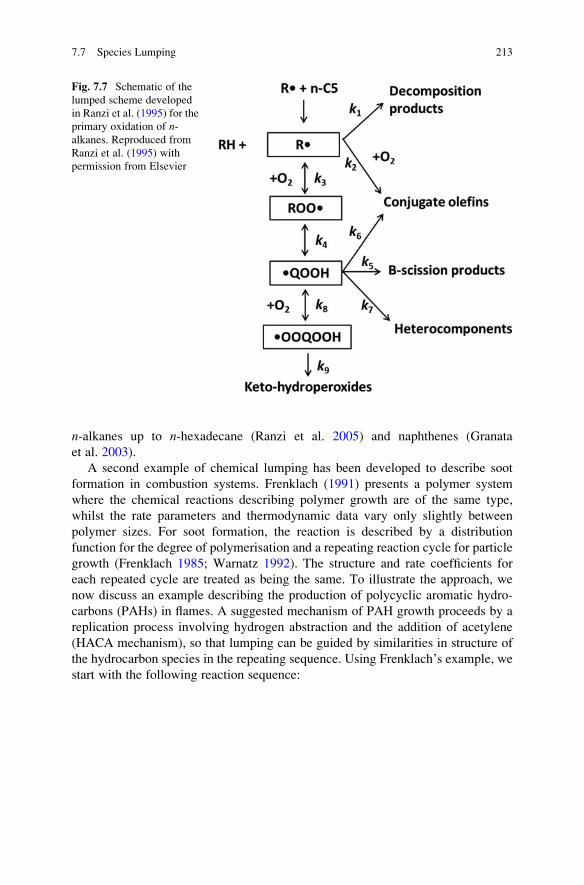
n-alkanes up to n-hexadecane (Ranzi et al. 2005) and naphthenes (Granata

et al. 2003).

A second example of chemical lumping has been developed to describe soot

formation in combustion systems. Frenklach (1991) presents a polymer system

where the chemical reactions describing polymer growth are of the same type,

whilst the rate parameters and thermodynamic data vary only slightly between

polymer sizes. For soot formation, the reaction is described by a distribution

function for the degree of polymerisation and a repeating reaction cycle for particle

growth (Frenklach 1985; Warnatz 1992). The structure and rate coefficients for

each repeated cycle are treated as being the same. To illustrate the approach, we

now discuss an example describing the production of polycyclic aromatic hydro-

carbons (PAHs) in flames. A suggested mechanism of PAH growth proceeds by a

replication process involving hydrogen abstraction and the addition of acetylene

(HACA mechanism), so that lumping can be guided by similarities in structure of

the hydrocarbon species in the repeating sequence. Using Frenklach’s example, we

start with the following reaction sequence:

Fig. 7.7 Schematic of the

lumped scheme developed

in Ranzi et al. (1995) for the

primary oxidation of n-alkanes. Reproduced from

Ranzi et al. (1995) with



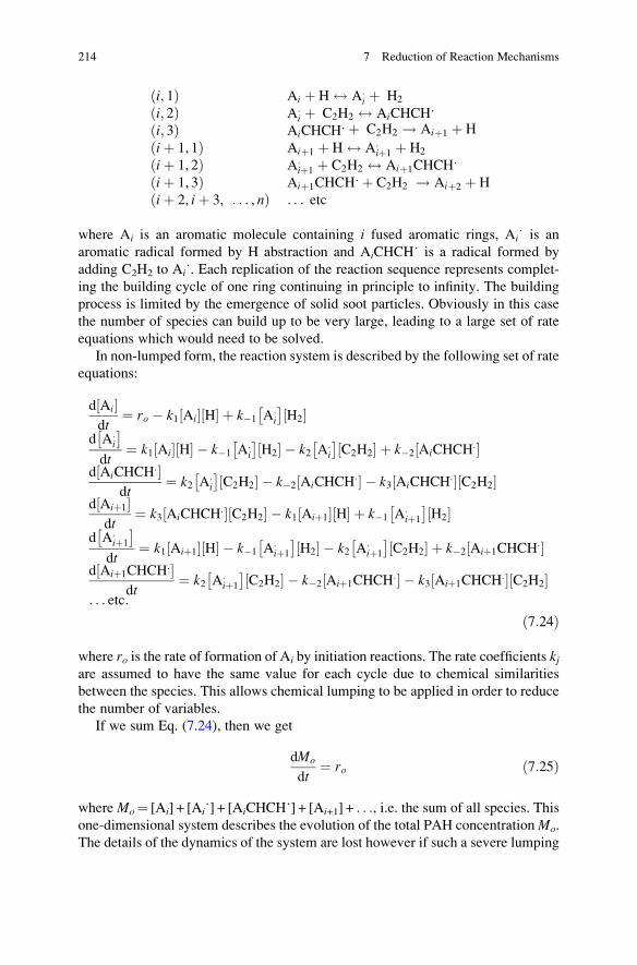
i; 1ð Þ Ai þ H $ A:i þ H2

i; 2ð Þ A:i þ C2H2 $ AiCHCH

:

i; 3ð Þ AiCHCH:þ C2H2 ! Aiþ1 þ H

iþ 1, 1ð Þ Aiþ1 þ H $ A:iþ1 þ H2

iþ 1, 2ð Þ A:iþ1 þ C2H2 $ Aiþ1CHCH

:

iþ 1, 3ð Þ Aiþ1CHCH:þ C2H2 ! Aiþ2 þ H

iþ 2, iþ 3, . . . , nð Þ . . . etc

where Ai is an aromatic molecule containing i fused aromatic rings, Ai˙ is an

aromatic radical formed by H abstraction and AiCHCH˙ is a radical formed by

adding C2H2 to Ai˙. Each replication of the reaction sequence represents complet-

ing the building cycle of one ring continuing in principle to infinity. The building

process is limited by the emergence of solid soot particles. Obviously in this case

the number of species can build up to be very large, leading to a large set of rate

equations which would need to be solved.

In non-lumped form, the reaction system is described by the following set of rate

equations:

d Ai½ �dt

¼ ro � k1 Ai½ � H½ � þ k�1 A:i

� H2½ �

d A:i

� dt

¼ k1 Ai½ � H½ � � k�1 A:i

� H2½ � � k2 A:

i

� C2H2½ � þ k�2 AiCHCH

:½ �d AiCHCH

:½ �dt

¼ k2 A:i

� C2H2½ � � k�2 AiCHCH

:½ � � k3 AiCHCH:½ � C2H2½ �

d Aiþ1½ �dt

¼ k3 AiCHCH:½ � C2H2½ � � k1 Aiþ1½ � H½ � þ k�1 A:

iþ1

� H2½ �

d A:iþ1

� dt

¼ k1 Aiþ1½ � H½ � � k�1 A:iþ1

� H2½ � � k2 A:

iþ1

� C2H2½ � þ k�2 Aiþ1CHCH

:½ �d Aiþ1CHCH

:½ �dt

¼ k2 A:iþ1

� C2H2½ � � k�2 Aiþ1CHCH

:½ � � k3 Aiþ1CHCH:½ � C2H2½ �

. . . etc:

ð7:24Þ

where ro is the rate of formation of Ai by initiation reactions. The rate coefficients kjare assumed to have the same value for each cycle due to chemical similarities

between the species. This allows chemical lumping to be applied in order to reduce

the number of variables.

If we sum Eq. (7.24), then we get

dMo

dt¼ ro ð7:25Þ

where Mo¼ [Ai] + [Ai˙] + [AiCHCH˙] + [Ai+1] + . . ., i.e. the sum of all species. This

one-dimensional system describes the evolution of the total PAH concentrationMo.

The details of the dynamics of the system are lost however if such a severe lumping


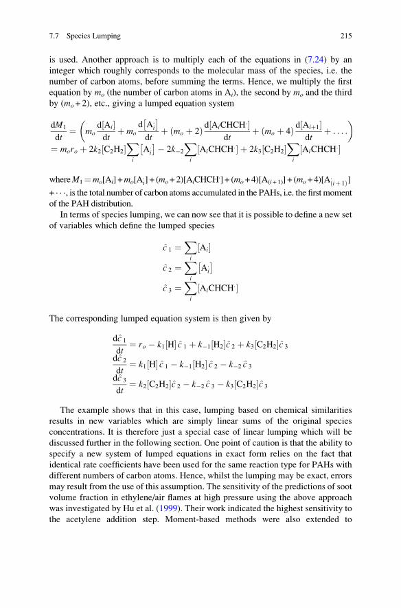
is used. Another approach is to multiply each of the equations in (7.24) by an

integer which roughly corresponds to the molecular mass of the species, i.e. the

number of carbon atoms, before summing the terms. Hence, we multiply the first

equation by mo (the number of carbon atoms in Ai), the second by mo and the third

by (mo+ 2), etc., giving a lumped equation system

dM1

dt¼ mo

d Ai½ �dt

þ mo

d A:i

� dt

þ mo þ 2ð Þ d AiCHCH:½ �

dtþ mo þ 4ð Þ d Aiþ1½ �

dtþ . . . :

� �¼ moro þ 2k2 C2H2½ �

Xi

A:i

� � 2k�2

Xi

AiCHCH:½ � þ 2k3 C2H2½ �

Xi

AiCHCH:½ �

whereM1¼mo[Ai] +mo[A:i] + (mo+2)[AiCHCH

.] + (mo+4)[A(i+1)] + (mo+4)[A:ðiþ 1Þ]

+ � � �, is the total number of carbon atoms accumulated in the PAHs, i.e. the first moment

of the PAH distribution.

In terms of species lumping, we can now see that it is possible to define a new set

of variables which define the lumped species

c 1 ¼Xi

Ai½ �

c 2 ¼Xi

A:i

� c 3 ¼

Xi

AiCHCH:½ �

The corresponding lumped equation system is then given by

dc 1

dt¼ ro � k1 H½ � c 1 þ k�1 H2½ �c 2 þ k3 C2H2½ �c 3

dc 2

dt¼ k1 H½ � c 1 � k�1 H2½ � c 2 � k�2 c 3

dc 3

dt¼ k2 C2H2½ �c 2 � k�2 c 3 � k3 C2H2½ �c 3

The example shows that in this case, lumping based on chemical similarities

results in new variables which are simply linear sums of the original species

concentrations. It is therefore just a special case of linear lumping which will be

discussed further in the following section. One point of caution is that the ability to

specify a new system of lumped equations in exact form relies on the fact that

identical rate coefficients have been used for the same reaction type for PAHs with

different numbers of carbon atoms. Hence, whilst the lumping may be exact, errors

may result from the use of this assumption. The sensitivity of the predictions of soot

volume fraction in ethylene/air flames at high pressure using the above approach

was investigated by Hu et al. (1999). Their work indicated the highest sensitivity to

the acetylene addition step. Moment-based methods were also extended to


modelling the dynamics of particle systems including coagulation/agglomeration in

Frenklach and Harris (1987), and Kazakov and Frenklach (1998).

Chemical lumping has also been applied within atmospheric mechanisms based

on a number of slightly different approaches. For example, within the tropospheric,

Master Chemical Mechanism (MCM), lumping is used in the case of peroxy

radicals to define the generic species ROO• (Saunders et al. 2003). The full

MCM, however, remains for the most part an explicit, detailed mechanism.

Reduced forms of the MCM were developed in the Common Representative

Intermediates (CRI) mechanism using lumping methods (Jenkin et al. 2008; Wat-

son et al. 2008). At the first stage, a version of structural chemical lumping is

applied based on the assumption that the ozone-forming potential of a volatile

organic compound (VOC) is related to the number of reactive bonds (i.e. C–C and

C–H) it contains. Based on structural similarities, a set of generic intermediates or

“common representatives” is then defined, each containing a large set of species

from the full MCM possessing the same ozone-forming index as the common

representative. At the second stage of reduction, the CRI mechanism uses a

surrogate approach, where the masses of minor VOCs are redistributed into a

much lower number of surrogate compounds. These surrogates are selected in

order to maintain the chemical class of the redistributed VOCs with the aim of

preserving the tropospheric ozone-forming ability of each category. Several differ-

ent levels of reduction were offered in Watson et al. (2008). When coupled with the

first reduction stage, over an order of magnitude reduction was achievable when

compared to the equivalent explicit MCM mechanism.

Lumping based on functional groups was also developed in Whitten

et al. (1980), Gery et al. (1989), Fish (2000), Yarwood et al. (2005) and Kirchner

(2005) as discussed in Sect. 3.1. In these approaches, each carbon atom is given a

type depending on the number of carbon atoms to which it is bonded and a status

depending on its functional group. Structural activity relationships are then used to

generate rate coefficients for the lumped groups, and the fraction of the original

VOCs within the lumped quantities is tracked.

Lumping is also associated with the so-called family method in atmospheric

chemistry (Crutzen 1971; Turco and Whitten 1974; Austin 1991; Jacobson 2005).

Here, the families of chemical species are defined not only on the basis of structural

similarity but also on other chemical reasoning such as reactivity. The approach has

tended to be used mostly in the context of fast numerical methods for solving ODEs

related to atmospheric chemical systems. It is based on the principle that for some

groups or “families” of species, atoms transfer quickly among species within the

family but are lost slowly from it (Jacobson 2005). For example, within the family

odd oxygen [OX]¼ [O] + [O(1D)] + [O3], the O atoms cycle rapidly between the

species atomic oxygen, excited atomic oxygen (O1D) and ozone but are slowly lost

from within this group. Similar groups exist for odd nitrogen (NOy), hydrogen

(HOx), bromine (Bry) and chlorine (Cly) species.

Using families within the solution to ODEs requires several steps. First, the rates

of production and loss of individual species are calculated from the initial concen-

trations, and then summed across a family. The family concentration is then



advanced to the next time step using something like a forward Euler approximation

(Elliott et al. 1993). In the final stage, individual species concentrations have to be

repartitioned within the family ready for the next time step. Several methods for this

repartitioning (a version of inverse lumping as discussed in the next section) can be

used, and the reader is referred to Jacobson (2005) for detailed examples. It is

important to note, however, that these usually have to invoke some kind of

approximation, such as the use of the QSSA, or a linearisation of the equations,

and hence, the family method can lead to numerical errors if family groupings are

not appropriately chosen. Austin, for example, discovered errors of order 20 % to be

induced in OH radical concentrations within photochemical stratospheric models

when too small a number of families were used (Austin 1991).

The errors induced within methods based on timescale separations will be

discussed in more detail in Sect. 7.8 below. On the other hand, since equilibrations

will exist within the groups, the introduction of such families is likely to lead to

the elimination of fast timescales, thus reducing the stiffness of the reduced system

of differential equations with resultant increases in simulation speed. O1D,

for example, has an atmospheric lifetime of the order of 10�8 s (see Sect. 6.3),

and therefore, its presence within a scheme can lead to large stiffness ratios when

treated as an individual species. Within reactive flow models, further computational

gains may also be made by advecting these families within the transport step rather

than individual species, thereby reducing the number of transported variables.

The family method was applied within an atmospheric chemistry box model to

NOy, HOx, Cly, Ox and Bry families in order to study the effect of increases in

ground level bromine emissions on stratospheric ozone by Ramaroson et al. (1992),

and for simulations of lower stratospheric HCl in Douglass and Kawa (1999). The

nonlinear features of tropospheric ozone production from nitrogen oxides and

VOCs were reproduced using a numerical method based on family methods in

Elliott et al. (1996).

Approaches to lumping in biochemical and systems biology applications tend to

be based on mathematical algorithms and will therefore be discussed after such

algorithms are introduced within the next section.

7.7.2 Linear Lumping

We saw in the previous section that chemical lumping is often based on defining

new species whose concentrations are linear combinations of those of the starting

species within a mechanism. This approach can be generalised within a mathe-

matical framework. The formal definition of lumping is the transformation of the

original vector of variables Y to a new transformed variable vector Y using the

transformation function h:



Y ¼ h Yð Þ ð7:26Þ

The dimension n of the new variable vector Y is smaller than that of the original

concentration vector ( n < NS ). Due to the transformation above, a new kinetic

system of ODEs is formed:

dY

dt¼ f Y; k

� �, Y t0ð Þ ¼ Y 0: ð7:27Þ

An important feature is the ability to recover the original vector of concentrations

from the transformed variables Y using the inverse transformation function h:

Y ¼ h Y� � ð7:28Þ

Function h is not unique, since several different functions h may belong to the

same transformation function h. This inverse mapping is as important as the

forward mapping not only because it provides the link between the lumped vari-

ables and the original species concentrations, but because its existence is a neces-

sary condition of exact lumping.

If the function h is linear, then in chemical kinetics, this approach would be

termed linear species lumping and is essentially a formalisation of the chemical

lumping approach described in the previous section. In the linear case the transfor-

mation is simply a matrix multiplication operation:

Y ¼ MY ð7:29Þ

where M is a matrix of size n � NS. Consider, for example, the following matrix:

M ¼ 1

0

0

1

0

1

0

1

� �: ð7:30Þ

This lumping matrix transforms an original concentration vector (Y1,Y2, Y3,Y4) to

the concentration vector Y1; Y2

� �of lumped species, where Y 1 ¼ Y1 and

Y 2 ¼ Y2 þ Y3 þ Y4.

Linear species lumping is called proper species lumping (Okino and

Mavrovouniotis 1998), if the concentration of each original species appears in the

transformation function of only one lumped species. If there are lumped species

present in a kinetic reaction mechanism, such a mechanism is called a lumpedreaction mechanism. In some cases, it is possible to regain the exact original

concentration vector after using the transformation in Eq. (7.26), solving the

differential Eq. (7.27) and then using the inverse transformation in Eq. (7.28).

This is the case when the lumping is based on conserved properties, and therefore,


no information is lost during lumping. This type of lumping is called exact specieslumping (Wei and Kuo 1969; Li and Rabitz 1989; Farkas 1999).

If we assume that the original kinetic system of differential equations contains

first-order reaction steps only, and therefore the concentration changes can be

described by the following initial value problem:

dY

dt¼ �KY, Y t0ð Þ ¼ Y0 ð7:31Þ

then linear species lumping results in the following different initial value problem:

dY

dt¼ �KY , Y t0ð Þ ¼ Y 0 ð7:32Þ

Wei and Kuo (1969) have shown that the necessary and sufficient condition of

exact linear lumping is the following equation:

MK ¼ KM ð7:33Þ

It is always possible to find matrices K and M that fulfil Eq. (7.33), but the

solution is not unique. The equivalent problem is finding invariant subspaces of the

original equations, i.e. invariant subspaces of the transpose of the Jacobian JT(Y) so

that the eigenvalues of JT(Y) and JT(M-1MY) are identical, which is fairly straight-

forward for this linear example where the Jacobian is a constant matrix. However,

this is often a difficult task for more general nonlinear ODEs where applying the

restrictions imposed by exact lumping may limit the level of reduction possible for

the reduced scheme.

We include here a short example of linear lumping taken from Li and Rabitz

(1989) in order to illustrate the approach. Consider the first-order reaction system

involving reversible reactions between three species as follows:

C1ÆC2, k1f ¼ 3, k1b ¼ 2

C2ÆC3, k2f ¼ 10, k2b ¼ 6

C1ÆC3, k3f ¼ 10, k3b ¼ 4

The corresponding kinetic equations are

dc1dt

¼ �13c1 þ 2c2 þ 4c3 ð7:34Þdc2dt

¼ 3c1 � 12c2 þ 6c3 ð7:35Þdc3dt

¼ 10c1 þ 10c2 � 10c3 ð7:36Þ

where the rate constants are essentially arbitrary numbers.


In vector form we can write this system as

dc

dt¼ Kc ð7:37Þ

Where K is the matrix of rate constants and

JT cð Þ ¼�13 2 4

3 �12 6

10 10 �10

0@ 1A ð7:38Þ

The eigenvector matrix X of JT(c) is given by

X ¼1 1 0:61 1 �0:41 �1 0

0@ 1A ð7:39Þ

Any subspace spanned by a subset of these eigenvectors will be JT(c) invariant and

could therefore form a suitable lumping matrix. For example, span (x1, x2) gives the

two-dimensional lumping matrix:

M ¼ 1 1 1

1 1 �1

� �ð7:40Þ

The lumped form of the equations is given by

dc

dt¼ MKc ð7:41Þ

However, in order to express the right-hand side in terms of the new lumped

variables c, then the generalised inverse M�1 needs to be found. The inverse will

not be unique, but its form does not affect the form of the lumped equations. We can

arbitrarily choose

M�1 ¼0:5 0

0:5 0

0 1

0@ 1A ð7:42Þ

and the lumped equations become

dc

dt¼ MKM�1 c ¼ �10 10

10 10

� �c ð7:43Þ

In this simple case, it is possible to interpret this as a lumped kinetic scheme


C 1ÆC 2

whereC 1 ¼ c1 þ c2 þ c3 andC 2 ¼ c1 þ c2 � c3. Of course the above example is for

a simple first-order system where an exact linear lumping approach can be applied.

Several developments of the lumping method have been proposed to help to

overcome the restrictions placed by exact linear lumping. The first is constrainedspecies lumping (Li and Rabitz 1991). Usually we are not interested in predicting

the concentrations of all species in the original kinetic system of ODEs, but only in

important ones such as key products or pollutants. In constrained lumping the

original vector of concentrations is rearranged so that the first n elements consist

of the concentrations of the n important species. Then, transformation h is selected

so that it does not change the first n elements of vector Y. Chu et al. (2011)

suggested a new algorithm for approximate, linear constrained lumping. Some

variables of the original model are selected to be retained in the lumped model,

whilst the other variables are lumped by linear combination. The technique is based

on the Petrov–Galerkin projection, and the projection matrix is computed from

simulation data obtained from the original model. The projection matrix is calcu-

lated in a computationally inexpensive way using a sequential algorithm based on a

modified Gram–Schmidt orthogonalisation procedure.

Other recent advances in the application of algorithmic methods for linear

lumping have attempted to develop methods that are based on formal mathematical

principles but do not lead to the stringent restrictions on the numbers of lumped

species achievable caused by the application of exact linear lumping methods.

Huang et al. (2005) defined a formal lumping procedure for intermediate species

where the fraction of each component within the lump αi (equivalent to the inverse

lumping matrix M ) is defined in terms of the fractional formation rate of the

components of the lump. The intention of the procedure is to suggest suitable

lumped groups whilst maintaining the flexibility required to model the conse-

quences of chemistry arising from reactions of the individual species within each

lump. The selection of suitable lumping groups is determined via the calculation of

the ratio of the normalised formation rates between candidate species i and

j denoted by γi,j. If the ratio is approximately constant over the course of the

simulation, then the two species can be lumped. The method was extended to larger

lumped groups. For example, for a lumped group containing three species A, B

and C, then α is calculated as follows:

αA ¼ RA

RA þ m1RB þ m2RC

αB ¼ m1RB

RA þ m1RB þ m2RC

αC ¼ m2RC

RA þ m1RB þ m2RC

ð7:44Þ

where Ri is the formation rate of species i,m1¼ γA,B,m2¼ γA,C and α1 + α2 + α3¼ 1.


The method was illustrated with respect to the simulation of higher hydrocarbon

generation during the isothermal oxidation of fuel-rich methane–oxygen mixtures,

where 31 species were lumped into nine groups giving a reduction in the number of

species of 22. In this application, the selection of groups is achieved by first

ordering the maximum gradients of the ratio γi,j over the simulation, given by φi,j.

The first group is then formed by selecting two species that have the lowest φi,j.

Other candidates are then tested for inclusion in this group by comparing φi,j values

with current members compared to a user-defined tolerance. When no further

candidates can be added, then two new starting candidates are selected from the

remaining ordered list, and the operation is continued until no further groups are

achievable. Integer programming methods could potentially be used to extend this

method to defining fully optimal lumped groups.

7.7.3 Linear Lumping in Systems with Timescale Separation

Other algorithmic methods for linear lumping have been developed for atmospheric

chemistry applications (Sportisse and Djouad 2000; Djouad and Sportisse 2002;

Djouad et al. 2003; Whitehouse et al. 2004c) but could potentially be relevant to

other types of chemical kinetic simulations. These methods have exploited a

timescale analysis in order to define lumped groups. For example, in Whitehouse

et al. (2004c), species are grouped according to their chemical lifetimes and

reactivity structures. This work applied the methods to the comprehensive tropo-

spheric Master Chemical Mechanism (MCM). Several large lumped groups were

achievable which were composed of peroxyacyl nitrates, nitrates, carbonates,

oxepins, substituted phenols, oxyacids and peracids with similar lifetimes and

reaction rates with OH. This approach could be considered as a formalisation of

chemical lumping where chemical similarities are not judged by expert opinion but

are calculated on the basis of reaction rates.

Djouad and Sportisse (Sportisse and Djouad 2000; Djouad and Sportisse 2002)

use lumping techniques based on the stoichiometric matrix of the fast subspace of

the system to define the partitioning between slow and fast species. The method is

equivalent to searching for slow species as linear combinations of fast ones and

is therefore aimed at reducing the stiffness of the modelling problem for use

with efficient numerical solvers. The approach also provides information on the

dynamic behaviour of the model and was successfully demonstrated for tropo-

spheric reaction systems including multi-phase applications (Djouad et al. 2003). It

should be pointed out that the wide applicability of simple linear algorithms for

lumping in atmospheric chemistry is in part due to the low-temperature dependence

of reaction rates for these schemes. Extension to non-isothermal systems would

provide an interesting area for further work.

We now briefly provide a formalised framework for linear lumping in systems

with timescale separation which is based on a similar approach to that presented in

Sect. 6.3. We start with the initial value problem



dY

dt¼ f Y; kð Þ, Y t0ð Þ ¼ Y0 ð7:45Þ

with the linear approximation to 7.45 given by

dY

dt¼ JY ð7:46Þ

where J is the Jacobian matrix. We can define new variables Z by choosing an

n� n-dimensional lumping matrix QT such that

Z ¼ QTY ð7:47Þ

The Schur decomposition is defined byQTJQ¼Twhere T is an upper triangular

matrix, QQT¼QTQ¼ I, and

Q ¼ q1 q2 . . . qnð Þ ð7:48Þ

where qi are the Schur basis vectors. The Schur decomposition (Golub and Van

Loan 1983) is used instead of applying the eigenvectors as a basis since it has more

general application to ill-conditioned matrices where degenerate eigenvalues may

exist (Maas and Pope 1992). Q can be chosen such that the eigenvalues of J appear

in any order along the diagonal of T and hence could be ordered according to fast

and slow timescales. If we choose QT such that the eigenvalues appear in

descending order on the diagonal, then

QTJQ ¼ J0 11ð Þ

J0 12ð Þ

0 J0 22ð Þ

!ð7:49Þ

where J0(11) corresponds to the n� n most negative eigenvalues (i.e. the fastest

relaxing timescales) and J’(22) corresponds to the n positive or small negative

eigenvalues. Therefore, the local linear system for Z is given by

dZ

dt¼ J

0 11ð ÞJ

0 12ð Þ

0 J0 22ð Þ

!Z ð7:50Þ

If a gap in timescales exists as discussed in Sect. 6.3, then the lumping matrix

can be partitioned as

QT ¼ QTf

QTs

� �ð7:51Þ

whereQTf is of dimension n� nð Þ � nand spans the space of the fast timescales.QT

s

is of dimension n � n and defines an n � n lumping matrix which spans the slow

subspace and determines the lumped variables. Z can therefore be partitioned as



Z ¼ F

S

� �ð7:52Þ

and the equations describing the linear system become

dF

dt¼ J

0 11ð ÞFþ J

0 12ð ÞS ð7:53Þ

dS

dt¼ J

0 22ð ÞS

The variables in the slow subspace S are therefore decoupled from those in the

fast subspace, and therefore, the lumping allows the definition of a reduced set of

variables S describing the longer timescale dynamics. The connections with the

slow manifold methods described in Sect. 6.5 also become clear since the calcu-

lation of the points on the manifold involves solving the following algebraic set of

equations:

QTf f Y; kð Þ ¼ 0 ð7:54Þ

We return to a discussion of numerical methods for solving such relationships in

Sect. 7.10.

7.7.4 General Nonlinear Methods

The methods of chemical and linear lumping outlined above can be extremely

effective for large systems where similarities in rate coefficients exist for chemi-

cally similar groups. However, they are difficult to extend in a general sense where

nonlinear couplings exist between groups of species. One solution may be to

consider the system as locally linear so that different lumping schemes are devel-

oped for different regions of composition space. However, one can imagine that for

highly nonlinear problems such as ignition or oscillatory systems, the lumping

transformations may vary rapidly, and the overhead in switching between different

lumped variables may outweigh any benefits gained from reducing the number of

variables. Methods for approximate nonlinear lumping have therefore been devel-

oped as discussed in the earlier review of Tomlin et al. (1997). Development of a

general nonlinear approach to lumping is, however, a non-trivial task. Instead of

simple matrix calculations, global canonical forms are now sought for the chemical

rate equations which separate the variables in a general way for many sets of

conditions. Nonlinear methods therefore may provide a more general approach

which is applicable over wider ranges of external conditions such as temperatures

and pressures, but this may be at the expense of algebraic complexity, since the

transformation from original to lumped variables is now of a nonlinear form.



The theory of nonlinear lumping has been developed by Li and co-workers who

started first by establishing necessary and sufficient conditions for exact nonlinear

lumping (Li et al. 1994a). Starting with the equation system (7.45), we can define

new lumped variables using a general n -dimensional nonlinear transformation to

new variables Y ¼ h Yð Þ with a new n -dimensional equation system given by

dY

dt¼ f Y tð Þ� � ð7:55Þ

If we define the Jacobian of the transformation h(Y) as Dh,c(Y)¼∂h/∂Y, then

Dh,c Yð Þf Yð Þ ¼ Dh,ch h Yð Þð Þf h h Yð Þð Þ� � ð7:56Þ

is a necessary and sufficient condition for exact lumping. In parallel to the linear

case, exact lumping depends on the existence of the generalised inverse trans-

formation h. Since h is now a nonlinear function, the calculation of h becomes

challenging for high-dimensional or highly coupled systems.

For easier comparison with the linear case, we can redefine the system using a

linear partial differential operator A, which, using index notation, is given by

A ¼Xni¼1

f i Y tð Þð Þ ∂∂Yi

ð7:57Þ

giving the original system of equations in the form

dY

dt¼ A Yð Þ ð7:58Þ

Therefore, finding the nonlinear transformation h depends on finding canonical

forms for the original operator A or on finding invariant manifolds of the original

system, i.e. the nonlinear equivalent of searching for canonical forms of the

Jacobian J (e.g. diagonal or upper triangular form) and its invariant subspaces.

The intention is that in the new canonical form, the corresponding differential

equations will be partially or completely decoupled. For example, the diagonal

form of a nonlinear operator with a basis of eigenfunctions φi(Y) and invariants

ωj(Y) would be as follows:

AXki¼1

λi ωð Þφi Yð Þ ∂∂φi Yð Þ ð7:59Þ

where the eigenvalues λi(ω) are the equivalent of the diagonal elements in the linear

case. Hence, one approach is to search for the eigenfunctions of A which relate to

eigenvalues which are no longer constant but are functions of Y(t) (Li et al. 1994a).Li et al. (1994a) have demonstrated that finding a full space of eigenfunctions for a

general nonlinear system is a difficult task. They therefore developed a nonlinear


lumping approach based on finding approximate canonical forms for

A (Li et al. 1994b, c). Again, if we think about the corresponding linear case, one

way of finding approximate invariant manifolds was to exploit the timescale

separation within the system. Similar approaches can be taken in the nonlinear

case (Li et al. 1993, 1994b) as will be discussed in the following section on

timescale-based reduction methods.

7.7.5 Approximate Nonlinear Lumping in Systemswith Timescale Separation

It was noted in the previous section that the approach taken for lumping based on

timescale separation is to seek a canonical form for the Jacobian which separates

the slow and fast subspaces for the variables. This type of approach can also be

pursued for nonlinear approximate lumping where approximate canonical forms are

now sought for the operator A (see Eq. (7.57)) which separate the slow and fast

variables. The approach is based on the application of algebraic methods in

nonlinear perturbation theory (Bogaevski and Povzner 1991; Li et al. 1993,

1994b, c). The aim is to find a suitable canonical form that separates the nonlinear

right-hand sides of the lumped kinetic equations into slow and fast components.

Therefore, the operator A is defined in the form

A ¼ A0 þ εA1 þ ε2A2 þ � � �; ð7:60Þ

where ε is a small parameter. Then, a special form is sought for the operator which

allows the separation of groups of slow and fast variables as in the case of ILDM

(see Sect. 6.5). If Ao is dominant in magnitude compared to other Ais and the leadingoperator Ao is already in a canonical form such as diagonal, triangular or a quasi-

linear one, then finding canonical forms for each of the Ai is an easier task than

finding a general canonical form. The approach developed by Li et al. was based on

algebraic methods in nonlinear perturbation theory (Bogaevski and Povzner 1991;

Li et al. 1993).

Using the algebraic method in nonlinear perturbation theory, it is possible to find

a transformation operator S such that the resultant operator

A ¼ e�SAeS ð7:61Þ

has a canonical form similar to Ao, and S is similarly expanded

S ¼ εS1 þ ε2S2 þ . . . ; ð7:62Þ

where all the Si operators are linear partial differential operators. The dependent

variables in the corresponding differential equation system for A will be partially or



completely decoupled, and hence, the differential equations for the new decoupled

variables form lower-dimensional lumped differential equation systems (Li and

Rabitz 1996b).

The use of nonlinear canonical forms provides advantages over linear lumping

methods since the lumped groups may be valid over large regions of composition/

temperature space. The methods essentially provide higher-order accuracy than

methods such as the QSSA albeit at the cost of potentially complex algebraic

manipulations in order to find the terms of the perturbation expansion. For

constrained nonlinear lumping, the dependent variables of the lumped model are

the same as the original ones. Thus, the solutions of the original variables of interest

can be obtained directly by solving a lower-dimensional lumped differential equa-

tion system. This approach has been successfully demonstrated for H2/O2 combus-

tion system including ignition (Tomlin et al. 1994) and oscillatory behaviour

(Li and Rabitz 1995). The method was further extended for H2/O2 and CO/H2/air

combustion cases in Li and Rabitz (1996a, 1997) to the “special perturbation

method” in an attempt to improve the accuracy of higher-order terms generated

by constrained approximate nonlinear lumping methods, which were shown to be

divergent in some cases. A correction term was added to the first-order term, and a

Shanks transformation (Shanks 1949) was then applied to improve the convergence

of the corrected first-order perturbation series. The method was shown to give very

good accuracy for both the isothermal and non-isothermal case studies in H2/O2 and

CO/H2/air combustion with the advantage of avoiding the derivation of higher-

order terms. The approximation is shown in both examples to be significantly more

accurate than lower-order expressions based on QSSA and pre-equilibrium approxi-

mations, particularly during the initial phase of the reaction trajectories. One of the

disadvantages of these methods is the complex algebraic manipulations that result

from couplings between the variables. In Li and Rabitz (1996b), the approach was

combined with numerical methods for solving the resulting complex algebraic

relationships making the method more applicable for complex, non-isothermal

reaction systems.

7.7.6 Continuous Lumping

Besides the lumping of species using discrete weighted sums, another method for

decreasing the number of species in a model is the introduction of continuousspecies (Aris and Gavalas 1966; Bailey 1972; Aris 1989; Astarita and Ocone 1992;Laxminarasimhan et al. 1996; Zhao et al. 2002). Such techniques are useful in

models of processes involving highly complex hydrocarbon mixtures such as

petroleum feedstocks, for example. Here, extremely large numbers of species

may be present, many of which can be ordered according to one of their chemical

or physical features. This feature then becomes a relatively simple function of the

ordering variable. For example, in a polymerisation system, the melting point and

the reactivity of the oligomers are a smooth function of the number of monomer


units in the oligomer species. If the kinetic system contains several ten thousands of

oligomers of different sizes, then it is not useful to calculate the concentrations and

properties of each of the oligomers separately. Another example is mixtures of

hydrocarbons containing many similar hydrocarbon molecules. In such systems the

discrete species can be represented by a continuum, and the lumping procedure

becomes a process of integration rather than summation. This approach of conti-

nuous species has found application in models of catalytic cracking (Weekman

1979; Cicarelli et al. 1992; Laxminarasimhan et al. 1996) and modelling the lique-

faction of coal (Prasad et al. 1986).

The reactivity and physical properties of continuous species are defined as a

function of a dimensionless variable x2 [0,1). This variable is usually related to a

measurable physical quantity, such as molecular weight or boiling point. The

fraction of a continuous species belonging to an interval of variable x can be

calculated by integrating the time-dependent probability density function ρ(x, t)over this interval. According to its definition, the integral of this pdf is unit over thewhole domain of definition of x at any time.

The rate equations for lumped mixtures will now be discussed. If we consider an

isothermal reaction system containing m different reactant types which react irre-

versibly with an n-th order rate, then the resulting rate equations become

dcidt

¼ �kicni ð7:63Þ

If the reaction order is assumed to be constant for all species, then the only species-

dependent parameter is ki, and hence, a species can be defined by its concentration

ci and its reactivity ki.For m discrete species, a reactant lump can be expressed as

C tð Þ ¼Xmi

ci ki, tð Þ ð7:64Þ

If m becomes sufficiently large, then k can be treated as a continuous function, and

the lump can be expressed in integral form

C tð Þ �ðkk�g k; tð Þdk ð7:65Þ

Here k_ and k are the lower and upper limits for the particular mixture. The product

g(k,t)dk is the total concentration of a species with rate constants between k and k+ dk, and should be interpreted as a concentration distribution function. As the

number of species within the mixture grows and approaches infinity, then the

separation between k_ and k becomes larger, and for convenience, it is assumed

that k_! 0 and k !1. This leads to the conventional form of the lumping

equation for continuous mixtures:


C tð Þ �ð10

g k; tð Þdk ð7:66Þ

Chou and Ho (1988) modified this approach slightly so that Eq. (7.66) is expressed

as an integral over reactivity k by taking into account the fact that the number of

reactant types per unit range of k can vary along the k axis. This leads to a modified

expression for the lumped concentration:

C tð Þ �ð10

c k; tð ÞD kð Þdk ð7:67Þ

with time dependence

dC

dt� �

ð10

D kð Þkc k; tð Þndk ð7:68Þ

Here, D(k) acts as a weighting factor which takes into account that in the discrete

system the ki’s may not be equally spaced along the k axis but will depend on the

type of feedstock to the reactor. An advantage of this approach is that rate

coefficients and physical properties can be measured at fixed points, and then the

appropriate function for k can be determined by fitting to these measured values.

If the continuous species participates in first-order reactions only, then it is easy

to calculate (Okino and Mavrovouniotis 1998) the total concentration of the

continuous species at each time point, as well as the pdf belonging to this time

and the mean values of physical properties. If the continuous species participates in

reactions other than first order, then general solutions do not exist, but solutions can

be derived for several special cases (Astarita and Ocone 1986; Ho and Aris 1987;

Astarita 1989; Astarita and Nigam 1989; Ocone and Astarita 1993).

7.7.7 The Application of Lumping to Biologicaland Biochemical Systems

Lumping methods have found a number of applications within biological and

biochemical systems although the methods are sometimes referred to as the

“zooming” of states. An overview of the suitability of lumping methods for such

types of models is provided within the review of Maria (2004). Both symbolic and

numerical methods for unconstrained and constrained lumping were developed in

Brochot et al. (2005) and were demonstrated for 2- and 6-compartment physio-

logically based pharmacokinetic (PBPK) models for 1,3-butadiene. Whilst sym-

bolic approaches were deemed to be useful for starting models with a low number

of variables, numerical methods were required for more complex models.


Sunnaker et al. (2010) developed a linear lumping approach with application to a

model predicting the observed behaviour of fluorescence emission in photo-

synthesis. Their approach was based on timescale separations within the system.

It has strong similarities with the “family” approach developed in atmospheric

systems (see Sect. 7.7.1), since the criteria used for lumping a group of states

include the reactions between them occurring on a much faster timescale than the

overall system timescale. Graph-based methods were used to identify components

within each lump. The approach was generalised for nonlinear systems in Sunnaker

et al. (2011) and includes methods to determine the inverse transformation, i.e. the

functional relationship between the lumped states and the original ones. The authors

claim that this makes the lumped model more easily interpreted from the biological

point of view. The definition of inverse transformations is based on assumptions

regarding the system dynamics that result in a sufficient number of equations being

linear so that an inverse transform can be defined. These assumptions are based on

the QSSA and on conservation relations that typically occur in models based on

mass action kinetics (as discussed in 2.3) and are common in models involving

transporters and enzymes. The method was demonstrated for a model describing

glucose transport across the cell membrane in baker’s yeast.The exploitation of timescale separation was also performed by Liao and

Lightfoot (1988) within a formal linear lumping approach similar to that outlined

in Sect. 7.7.3. They demonstrated the approach for the red cell glycolysis model for

which the original system has 15 variables. They show that with different degrees of

lumping or “zooming”, the reduced model is able to represent the system dynamics

on different timescales. For example, the lumped 2 variable model describes the

system dynamics for timescales longer than an hour, but 4 additional variables are

needed to capture the dynamics on the timescale of minutes. Such “time hierar-

chies” in biological systems were also discussed by Maria (2006), particularly with

respect to genetic regulatory network (GRN) models (Maria 2008, 2009). Maria

argues that the level of detail within lumped sub-modules should be adjusted

according to the available experimental information which is perhaps important

for parameter estimation problems. Brochot et al. (2005) suggest that the use of

lumping to develop reduced models can assist in overcoming problems of statistical

identifiability within parameter estimation for pharmacokinetic models. For exam-

ple, when model parameters are highly correlated or have multiple peak posterior

distributions, parameter estimation can require a large number of runs in order to

explore the space of possible parameter values. A reduced model is therefore

computationally beneficial. However, Maria warns that the application of lumping

to models of metabolic processes must account for the physical significance of

species and their interactions, as well as the systemic properties of the metabolic

pathway, rather than being based on purely mathematical analysis of system

timescales (Maria 2006). One important aspect of lumping in biological and

biochemical systems therefore, may be the need to relate the lumped parameters

and variables back to those of the original model.

Dokoumetzidis and Aarons (2009b) further highlight the need for variables and

parameters within reduced biological models to retain a specific physiological


meaning. They develop an approach for proper lumping, where each of the original

species contributes to only one of the pseudo-species within the lumped system,

meaning that the original species form groups which have a clear physical inter-

pretation. Their algorithm is based on a formal lumping approach as outlined in

Sect. 7.7.2. Many possible lumping matrices are explored, and an optimisation

approach is used to select the reduced model with the smallest error when compared

to the original model. To avoid a combinatorial explosion (see Sect. 7.6), the lumps

are added one at a time in a greedy-type approach. However, for a system with

30 variables and 20 lumps, over 8000 model evaluations are still required. The

approach was demonstrated for a model describing the signalling pathways of

NF-κB. A useful development to this approach was made in Dokoumetzidis and

Aarons (2009a) where parameter uncertainties were accounted for. Here a Bayesian

framework was used to produce lumping schemes which, whilst not necessarily

optimal for the nominal parameter values, were optimal on average over the prior

parameter distribution (i.e. incorporating uncertainties). This was compared with a

standard non-Bayesian lumping method which produced a model that was good for

the nominal values but was very poor for other values within the prior distribution.

The approach was demonstrated for a physiologically based pharmacokinetic

(PBPK) model for barbiturates. Their study raises the very important issue of

model reduction under uncertainty which is particularly critical if the reduced

model is to be used within the context of parameter estimation.

An algorithm for lumping coupled with parameter optimisation and variable

elimination was also developed in Dano et al. (2006) and demonstrated for a

20-variable model of yeast glycolytic oscillations. A key aim of their approach is

to ensure that the lumping and reduction procedures preserve the dynamic behav-

iour of the model, an issue which was also discussed more formally in Toth

et al. (1997). The model was first lumped using a method similar to Sunnaker

et al. (2010), and then parameter optimisation was performed in order to preserve

the dynamic properties of the model such as its oscillatory behaviour and the

structure of the bifurcation diagram. Variables are then eliminated from the

dynamic model using QSSA relationships, and an optimisation approach is also

used to test all physically realistic models and to search for the smallest one which

preserves the dynamic behaviour of the model. The combinatorial explosion which

is typically found in optimisation problems (Sect. 7.6) is avoided by sequentially

applying the QSSA to the least important species until the point at which the

oscillatory behaviour is lost upon further elimination. This type of methodology

would be greatly assisted by formalised methods for the selection of QSS-species

which will be discussed in the following section.

7.8 The Quasi-Steady-State Approximation

We hinted in Sect. 2.3.6 that the timescale separation present in most kinetic

systems can be exploited in terms of model reduction. The next sections will

therefore cover the use of timescale analysis for the reduction of the number of

7.8 The Quasi-Steady-State Approximation 231


variables within kinetic models. This can have the added advantage of reducing the

stiffness of the equation systems (see Sect. 6.7), since often the fast variables are

removed from the system of differential equations and determined through alge-

braic relations with respect to the slower variables. We start first with the appli-

cation of the QSSA, which is one of the simplest methods for exploiting timescale

separation and is based on associating fast and slow timescales to individual species

(see Sect. 6.3 for a full discussion of this point).

7.8.1 Basic Equations

Consider the following general initial value problem:

dY

dt¼ f Y; pð Þ, Y 0ð Þ ¼ Y0 ð7:69Þ

On applying the QSSA, we define non-QSSA variables (the slow variables) andQSSA variables (the fast variables) as Y¼ (Y(1), Y(2)). The distinction between fast

and slow variables was discussed in Chap. 6. The right-hand side of the system of

ODEs (7.69) can be divided accordingly: f¼ (f(1), f(2)). The concentrations of the

non-QSS-species are calculated by solving the system of ODEs f(1), whilst the

concentrations of the QSS-species are calculated by solving the algebraic system of

equations obtained by setting the right-hand side of equations f(2)to zero:

dY 1ð Þ

dt¼ f 1ð Þ Y; pð Þ, Y 1ð Þ 0ð Þ ¼ Y

1ð Þ0 ð7:70Þ

0 ¼ f 2ð Þ Y; pð Þ ð7:71Þ

The system of differential (7.70) and algebraic (7.71) equations is coupled through

common variables and therefore can only be solved together. Various numerical

methods exist for directly solving such differential algebraic equations (DAEs)

(Gear and Petzold 1984), although other tricks can be introduced to improve the

numerical efficiency of employing the QSSA as discussed below.

Application of the QSSA is successful if the solution of ODE (7.69) is almost

identical to the solution of the coupled DAEs (7.70 and 7.71). What is considered as

“almost identical” may depend on the actual problem and the accuracy required, but

in reaction kinetic modelling, a 1 % error for all species at any time is usually

considered acceptable. It was emphasised in Sect. 7.2 that the aim of chemical

kinetic simulations is the accurate calculation of the concentrations of important

species or those of important reaction features. Therefore, the statement above can

be refined so that the application of the QSSA is successful if the solutions of

Eqs. (7.69) and (7.70–7.71) are almost identical considering the concentrations of

important species and the important features.




http://dx.doi.org/10.1007/978-3-662-44562-4_6

7.8.2 Historical Context

The first application of the QSSA is usually attributed to Bodenstein (Bodenstein

1913; Bodenstein and Lutkemeyer 1924), but Chapman and Underhill (1913) and

Semenov (1939, 1943) were also early users of the technique. Further pioneers of

the application of the QSSA are Michaelis and Menten (1913) and Briggs and

Haldane (1925). The history of the application of the QSSA can be divided into

three periods (Turanyi et al. 1993b). In the early period (1913–1960), accurate

experimental data for various applications were obtained and compared with

solutions of simple kinetic systems of differential equations that were formulated

to model the experimental behaviour. Due to the limited availability of computer

power during this time, the kinetic ODEs had to be solved analytically and using the

QSSA helped to convert the systems into an analytically solvable form.

From the 1960s onwards, computers became available for many researchers, but

the stiff systems of ODEs that describe many kinetics applications often could not

be simulated using available computer codes during this early period of numerical

analysis. By applying the QSSA, the stiff systems of ODEs could be converted to

non-stiff ones (Snow 1966; Blouza et al. 2000), and numerical solutions to these

ODEs could be obtained using traditional ODE solvers.

The publication of the Gear algorithm (Gear 1971) allowed the numerical

solution of stiff systems of differential equations and facilitated the comparison

of solutions of the kinetic system of differential equations with and without the

application of the QSSA. In early numerical experiments, the two solutions were

often different, and therefore, Edelson et al. demanded the cease of the application

of the QSSA (Edelson 1973; Farrow and Edelson 1974). However, the QSSA is still

widely used (Mendiara et al. 2004; Machrafi et al. 2005; Strohle and Myhrvold

2006; Ciliberto et al. 2007) for the interpretation and simplification of reaction

mechanisms and speeding up reaction kinetic simulations. Peters et al. (Peters

1985; Paczko et al. 1986; Peters and Kee 1987; Peters and Rogg 1993) simplified

several detailed combustion mechanisms to skeleton mechanisms with only 2� 4

lumped reaction steps by using the QSSA, allowing the early use of combustion

kinetics in 3D computational fluid dynamic (CFD) simulations with complex

geometries. The explicit or hidden application of the QSSA is present in thousands

of articles on chemical kinetic modelling, and there are more than one hundred

articles dealing with the theory of the QSSA (see e.g. Miller and Alberty 1958;

Segel 1988; Segel and Slemrod 1989; Borghans et al. 1996; Tzafriri and Edelman

2004, 2005; Flach and Schnell 2006; Li et al. 2008a; Goussis 2012; Li and Li 2013).

It is a commonly used technique with perhaps a large potential for model reduction,

and therefore, it is worthwhile establishing sound principles on which to base its

application. Early failures of the application of the method are more likely to be due

to its inappropriate use, rather than a breakdown of the technique itself.


7.8.3 The Analysis of Errors

Several early articles dealt with the applicability of the QSSA for certain groups of

species. Detailed reaction mechanisms were simulated with and without the appli-

cation of the QSSA (see e.g. Farrow and Edelson 1974; Sundaram and Froment

1978; Savage 1990), and the two solutions were compared. This determines the

applicability of the QSSA for a given system at given conditions, but unfortunately

does not provide general conclusions. In other publications, the applicability of the

QSSA was investigated for small skeleton models such as the Michaelis�Menten

scheme (see e.g. Georgakis and Aris 1975) and on the basis of singular perturbation

theory (see the review of Klonowski (1983)). The main result of the latter approach

is that using the Tihonov theorem (Tihonov 1952; Heineken et al. 1967; Vol’pertand Hudjaev 1985), a necessary condition can be given for the applicability of the

QSSA. However, this theory cannot be applied for the calculation of the error

induced by the application of the QSSA for an arbitrary reaction mechanism which

will be covered below.

An early article on the error caused by the application of the QSSA was written

by Frank-Kamenetskii (1940), who is perhaps better known for theories on reactor

stability and flame modelling. This very brief article received only a few citations

over several decades following its publication (Benson 1952; Sayasov and

Vasil’eva 1955; Rice 1960). Turanyi and Toth (1992) published an English trans-

lation of Frank-Kamenetskii’s article with detailed comments. Further development

and generalisation (Turanyi et al. 1993b) of the reasoning of Frank-Kamenetskii

allows the calculation of the error caused by the QSSA and is detailed below.

On the application of the QSSA and using the notation introduced in Sect. 7.8.1,

the Jacobian can be divided into four submatrices:

J ¼ J 11ð Þ J 12ð Þ

J 21ð Þ J 22ð Þ

� �¼

∂f 1ð Þ

∂Y 1ð Þ∂f 1ð Þ



∂Y 2ð Þ

0BB@1CCA ð7:72Þ

At the beginning of reaction kinetic simulations, usually the concentrations of only

a few species (e.g. reactants, diluent gases, etc.) are defined, and other concen-

trations are set to zero. The QSSA is not usually applicable from the beginning of

the simulation since at this point, the trajectories are quite far from any underlying

slow manifolds (see Sect. 6.5). Hence, the kinetic system of ODEs (7.69) is usually

solved first, and at time t1 is switched to the solution of the DAE system (7.70–

7.71). We denote Y(t1)¼(Y(1)(t1), Y(2)(t1)) to be the solution of Eq. (7.69) at time t1.

When the system of Eqs. (7.70–7.71) is used, then the concentrations of the

QSS-species are calculated first via the solution of algebraic system of

Eqs. (7.71), and the result is concentration vector y(2)(t1). The concentrations of

the non-QSS-species are identical to the solution of system of ODEs (7.69) at time



t1, and therefore vector y(t1)¼ (Y(1)(t1), y(2)(t1)) is the initial value of the DAE

system of Eqs. (7.70–7.71).

The local error of the QSSA at time t1 is given by the following vector (Turanyiet al. 1993b):

Δy 2ð Þ t1ð Þ ¼ y 2ð Þ t1ð Þ � Y 2ð Þ t1ð Þ ð7:73Þ

We now calculate the Taylor expansion of function f(2) at variable values y(t1):

dY2ð Þi

d tt1ð Þ ¼ f

2ð Þi Yð Þ

h iY¼y t1ð Þ

þXk

∂f 2ð Þi Yð Þ∂Yk

" #Y¼y t1ð Þ

ΔY 2ð Þk t1ð Þ ð7:74Þ

where the expansion is applied for the QSSA variables only. Since vector y(t1) is a

root of the system of algebraic Eqs. (7.71), then f2ð Þi Yð Þ

h iY¼y t1ð Þ

¼ 0 for each i.

The second- and higher-order terms in the Taylor expansion are neglected. This is a

usual step in physical chemical derivations, but in this context it is justified, since if

the mechanism contains not more than bimolecular steps and does not contain

second-order consumption steps such as the reaction type 2A!B, then the third

and higher terms of the Taylor expansion are all zero.

Equation (7.74) can also be written in matrix form:

dY 2ð Þ

d t¼ J 22ð ÞΔy 2ð Þ ð7:75Þ

where dY(2)/d t is the production rate of the QSS-species at time t1 and J(22) is the

submatrix of the Jacobian belonging to the QSS-species at values y(t1). It is more

practical, however, to evaluate the matrix J(22)for the concentration vector Y(t1),which results in an almost identical matrix. If the production rate dY(2)/d t of the

QSS-species and matrix J(22)are known, then the local error Δy(2) of the QSSA at

any time t1 can be calculated by solving the algebraic system of Eq. (7.75).

The local error of the QSSA is not equal to the difference between the solution of

the systems of Eqs. (7.69) and (7.70–7.71) at later times, which we call the globalerror of the QSSA (Turanyi et al. 1993b). If the local error is large at the initial

time, then the initial condition of Eqs. (7.70–7.71) will be wrong, and therefore, the

global error is also expected to become large over time. In addition, if the agree-

ment between Eqs. (7.69) and (7.70–7.71) is good until time t2 and then the local

error suddenly increases, the global error may also become large over time. This

implies that successful application of the QSSA (i.e. where the global error is well

controlled) means that the local error should remain small during the whole interval

of its application.

Using the algebraic system of Eq. (7.75), the local error can be calculated for all

QSS-species. If this equation is used for species i only, the following equation is

obtained:


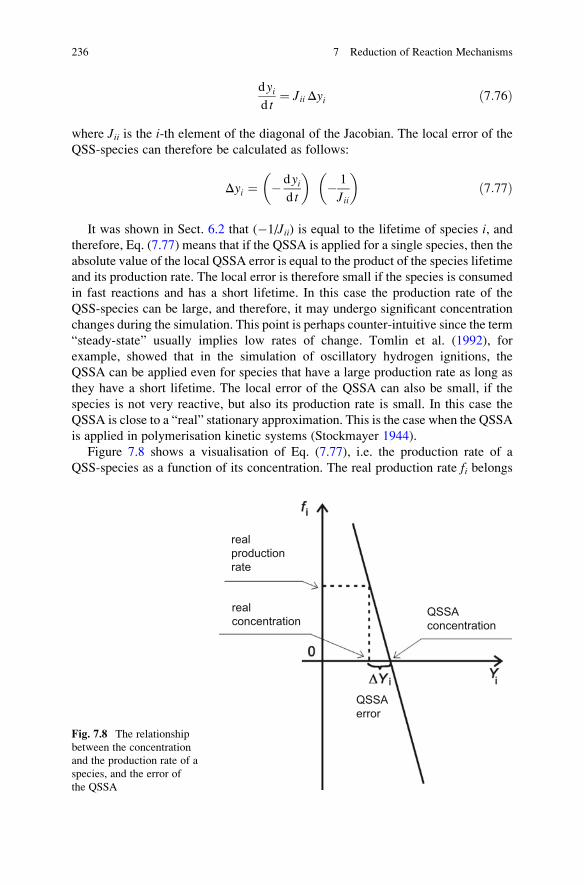
dyid t

¼ JiiΔyi ð7:76Þ

where Jii is the i-th element of the diagonal of the Jacobian. The local error of the

QSS-species can therefore be calculated as follows:

Δyi ¼ � dyid t

� �� 1

Jii

� �ð7:77Þ

It was shown in Sect. 6.2 that (�1/Jii) is equal to the lifetime of species i, andtherefore, Eq. (7.77) means that if the QSSA is applied for a single species, then the

absolute value of the local QSSA error is equal to the product of the species lifetime

and its production rate. The local error is therefore small if the species is consumed

in fast reactions and has a short lifetime. In this case the production rate of the

QSS-species can be large, and therefore, it may undergo significant concentration

changes during the simulation. This point is perhaps counter-intuitive since the term

“steady-state” usually implies low rates of change. Tomlin et al. (1992), for

example, showed that in the simulation of oscillatory hydrogen ignitions, the

QSSA can be applied even for species that have a large production rate as long as

they have a short lifetime. The local error of the QSSA can also be small, if the

species is not very reactive, but also its production rate is small. In this case the

QSSA is close to a “real” stationary approximation. This is the case when the QSSA

is applied in polymerisation kinetic systems (Stockmayer 1944).

Figure 7.8 shows a visualisation of Eq. (7.77), i.e. the production rate of a

QSS-species as a function of its concentration. The real production rate fi belongs

QSSAconcentration

realproductionrate

realconcentration

QSSAerror

Fig. 7.8 The relationship

between the concentration

and the production rate of a

species, and the error of

the QSSA



to the real concentration Yi(t1), whilst the zero production rate belongs to the QSSAconcentration yi(t1), calculated from Eq. (7.71). The figure shows that if function

fi(Yi) is steep, that is, slope �Jii is large (and hence the species lifetime is short),

then the deviation between the real and the approximated concentrations is small.

This means that the local error of the QSSA will be small, even if the real

production rate of the QSS-species is large. If the production rate of the

QSS-species is small, then the local error can be small, even if the slope of function

fi(Yi) is small. If the production rate is zero, then we apply the real steady-state

approximation instead of the QSSA. Several reaction kinetics textbooks claim that

the algebraic system of Eqs. (7.70–7.71) is applicable for the calculation of the

concentration of the QSS-species because the production rate of the QSS-species is

really almost zero. As Fig. 7.8 shows, the quasi-steady-state approximation is

successful if the real and the approximated concentrations are close to each other,

and it might be true even where the production rate is large, if function fi(Yi) is verysteep.

If any of the initial concentrations of intermediate species within the mechanism

are zero, then the QSSA is usually only applicable after a time duration called the

induction period. Using the equations above, the induction period can be estimated

to be about ten times the lifetime of the QSS-species with the longest lifetime

(Turanyi et al. 1993b).

The selection of QSS-species is perhaps the most important part of the appli-

cation of the QSSA. The following algorithm was suggested in Turanyi

et al. (1993b). First using Eq. (7.77), the local error of the QSSA (related to each

species separately) is calculated across the domain of application. A group of

candidate QSS-species is selected according to a user-defined tolerance. Up to

10 % error has been suggested to be tolerable within applications in combustion

(Hughes et al. 2009). Then local error is calculated for this group of species using

Eq. (7.75). If the approximated local error remains small, then the QSSA is applied

for this group of species (Whitehouse et al. 2004a, b). The selection can be checked

by comparing the solutions of systems of Eqs. (7.69) and (7.70–7.71), for the

important species and important features over selected conditions. DAE solvers

such as DASSL can be used for this purpose (Maly and Petzold 1996).

Due to the local error of the QSSA, the concentrations of the QSS-species

calculated by Eq. (7.70–7.71) are slightly different from the “real” concentrations,

which can be considered as a continuous perturbation of the trajectory of the

non-QSS-species. Using the Green function (see Sect. 5.2.3), or in other words

the initial concentration sensitivities, it is possible to assess (Turanyi et al. 1993b)

whether the concentration perturbation causes a significant deviation in the trajec-

tories of the non-QSS-species.



7.8.4 Further Recent Approaches to the Selectionof QSS-Species

As discussed in Sect. 2.3.5, conserved properties result in the linear combination of

species concentrations or other variables of the system remaining constant through-

out the trajectory. Such constants are called first integrals in mathematics. As

Straube et al. (2005) demonstrated, the presence of QSSA relations leads to further

linear functions of the concentrations being approximately constant during the

solution of the kinetic system of ODEs. Straube et al. called these functions

quasi-integrals. This means that identification of QSS-species can be based on the

identification of the corresponding quasi-integrals. The unique feature of this

approach is that in this case, the identification of the QSSA relations is not directly

based on the investigation of timescales.

The relationship between the QSSA and the calculated concentrations of the

important species was handled in a different way by Løvas and co-workers (Løvas

et al. 2000, 2002a, b; Løvas 2009), who introduced the level of importance (LOI)

index. This index is the product of the lifetime of a species and a local sensitivity

term:

LOIð Þij ¼ ϑiXNR

l¼1

νjl∂Yi

∂lnAlð7:78Þ

The summation refers to all the NR reaction steps. For the calculation of lifetime ϑi,not only the chemical lifetime τi is taken into account but also the residence time in

a reactor and the species’ rate of diffusion. The half-normalised local sensitivity

coefficient ∂Yi/∂ lnAl shows the effect of perturbing the A-factor of reaction step

l on concentration Yi, and νij is the corresponding stoichiometric coefficient.

The index (LOI)ij estimates the error of the calculation of the concentration of

species j due to the application of the QSSA on species i.According to Løvas and co-workers (2002a), a species having a short lifetime is

related to a small local error of the QSSA, but this small error may cause large

errors in the simulated concentrations if these species exhibit large sensitivities. In

several combustion systems, the QSSA error of the H-atom has such a property. In

this case the LOI is large, and the QSSA is not applicable for such a species as found

also in Tomlin et al. (1992). The opposite situation may arise when the species has a

long lifetime, therefore a large local QSSA error, but this large error does not spread

to the simulation results. An example might be that in ethylene/air and ethane/air

premixed flames, the molecule C2H2 can be treated as a QSS-species (Wang and

Rogg 1993). In this case the LOI is small, and the QSSA is applicable for this

species. The LOI seems to be practically useful and has been applied to

several systems. A mathematical derivation of the approach would be a useful

development.



Montgomery et al. (2006) used a genetic algorithm for the selection of

QSS-species. Based on the difference between the simulation results without and

with the application of the QSSA, the selection of the QSS-species was optimised

until the simulation error decreased below a certain threshold. CSP analysis can

also be used for the selection of QSS-species and is covered in more detail in Sects.

6.4 and 7.9. The validity of the QSSA in solution-phase bimolecular reactions was

also studied in Tzafriri and Edelman (2005).

Vora and Daoutidis (2001) developed a nonlinear model reduction method for

non-isothermal reaction systems that exhibit dynamics on two different timescales.

The method identifies the independent algebraic constraints (possibly of QSSA

origin) that define the low-dimensional state space where the slow dynamics of the

reaction system are constrained to evolve.

7.8.5 Application of the QSSA in Spatially DistributedSystems

The propagation of errors in spatially distributed systems is also important and has

been the subject of several studies. Yannacopoulos et al. (1996a, b) carried out a

mathematical study of the general case and found that in common with the spatially

homogeneous case, the higher the net rate of production of the QSS-species, the

larger the possible error. Steep spatial gradients in concentrations also led to larger

overall errors. They also state that the higher the minimum diffusion rate of the

species, the lower the possible error, which relates to the idea that steep spatial

gradients (and therefore large errors) are smoothened by strong diffusion processes.

In Yannacopoulos et al. (1995), a method was suggested to describe the transient

relaxation to the slow manifold (i.e. the induction period) based on algebraic sets

and perturbation theory. Its application was demonstrated for a simple enzyme

substrate model and a two-dimensional oscillatory system as well as spatially

distributed systems. The method is equivalent to finding higher-order approxi-

mations to the fast dynamics of the system, whereas the QSSA represents a

zeroth-order approximation. The additional accuracy of the higher-order approxi-

mation was found to reduce the propagation of errors in reaction–diffusion systems.

The main reason for this is a better approximation to the initial stages of the fast

dynamics during the induction period where the QSSA errors may be higher.

Although it was stated above that the QSSA should not be applied during this

induction period, in practice it is often applied during this period for spatially

homogeneous systems with little consequence on the long time errors. However,

because of the spatial dependence of the solution in reaction–diffusion systems,

transient dynamics before relaxation to the slow manifold can have a very impor-

tant effect on the solution at long times. In these types of cases, it is important to

find a reduced system which is a good approximation to the full system almost

everywhere, i.e. it is necessary to take into account the transient dynamics of the



relaxation to the slow manifold explicitly using higher-order approximations

(Yannacopoulos et al. 1995). Other methods for determining higher-order approx-

imations have been developed based on nonlinear perturbation theory as discussed

in Sect. 7.7.5.

7.8.6 Practical Applications of the QSSA

The classical textbook approach to the application of the QSSA is to describe the

concentrations of QSS-species via explicit algebraic expressions as functions of the

slower species. When the QSSA is used only for a few species or the QSS-species

are not strongly coupled to each other, then it is usually possible to calculate their

concentrations sequentially, in an order that allows explicit equations to be

obtained. Historically the QSSA was applied by directly solving such algebraic

expressions (e.g. Peters and Williams 1987); however, this often resulted in large

simplifications of the starting schemes to facilitate analytical solutions or truncation

of the QSSA expressions. Since we are now moving towards modelling more and

more complex systems, it is unlikely that these traditional methods will find general

application. On the other hand, Hughes et al. (2009) demonstrated that such an

approach based on algebraic equations could be applied to highly complex hydro-

carbon oxidation schemes when algebraic manipulation packages such as MAPLE

(Maple) are employed in order to provide a level of automation to the procedures. In

their approach the use of explicit expressions to describe the concentrations of the

QSS-species was coupled with reaction lumping in order to directly remove the

QSS-species from the reaction scheme. A simple example of this type of reaction

lumping based on the QSSA was demonstrated in Sect. 2.3.4 and showed that the

lumped rate parameters derived in this way are often complicated nonlinear func-

tions of the original rate parameters. They do not necessarily correspond to those of

a single rate-determining step, and hence, the approach is slightly more complex

than that described in Sect. 2.3.3.

Hughes et al. (2009) demonstrated the application of this approach for the

reduction of a skeletal scheme describing the oxidation of n-heptane from 218 spe-

cies to 110 species which is a substantial reduction. This extensive application was

possible since often in hydrocarbon oxidation schemes in both combustion and

atmospheric applications, the QSS-species are present in parallel pathways with

little coupling between them. Therefore, finding analytical solutions is possible

with the aid of algebraic manipulation packages. The types of species which can be

removed tend to be fast radicals such as alkyl radicals, alkyl hydroperoxy radicals

and hydroperoxyalkyl peroxy radicals (Hughes et al. 2009). Peroxy radicals, how-

ever, are shown to have higher QSSA errors and are often rate determining. They

therefore cannot be removed using the QSSA. A similar approach was also taken by

Whitehouse et al. within application to the Master Chemical Mechanism (MCM)

describing tropospheric hydrocarbon degradation (Whitehouse et al. 2004c). It

should be pointed out that such a simple approach is very difficult to apply to




highly coupled QSS-species and so may not be applicable to all possible

QSS-species.

In fact in general, the QSSA results in implicit nonlinear algebraic equations

(Pantea et al. 2014), the solution of which may require significant CPU time. It is

possible to solve the coupled DAE system using easily available numerical methods

such as DASSL as discussed above, but since this does not lead to substantial CPU

savings, the use of such an approach is usually confined to testing the validity of

applying the QSSA to selected groups of species over limited sets of conditions.

Numerical schemes based on the QSSA have also been developed as discussed in

Sandu et al. (1997a, b) and Jay et al. (1997). However, since the performance of

traditional QSSA solvers was worse than many of the other explicit and implicit

methods for solving the stiff atmospheric systems tested, we do not discuss them in

detail here, and refer the reader to the papers of Sandu and co-workers for further

details. A higher-order extension was also proposed in Jay et al. (1997), which was

shown to improve upon earlier schemes.

In general, larger CPU savings will be made by solving for the QSS-species

separately and substituting their concentrations into the ODEs for the slow species.

Methods based on either inner or fixed point iteration methods (see e.g. Chap. 6 in

Peters and Rogg 1993) or matrix manipulations (Chen 1988) have often been used

in the past. The former of these methods uses iteration cycles to solve the coupled

implicit equations, whereas the latter relies on matrix manipulations. The formu-

lation of these methods is discussed in Jay et al. (1997), and they have been

commonly applied in atmospheric chemistry (Jay et al. 1997) and combustion

(Løvas et al. 2002b). Chen and Tham (2008) elaborated a method for the effective

solution of the system of algebraic equations resulting from the QSSA. They stated

that neither fixed point iteration nor matrix inversion methods are generally effec-

tive. They identified the strongly coupled QSS-species first, and their concen-

trations were calculated using matrix inversion. Fixed point iteration was used for

the calculation of the concentrations of the other QSS-species. Also, if a nonlinear

system of algebraic equations has polynomial equations on the right-hand side, then

a numerically efficient way of solving it is to transform its coefficient matrix to an

upper triangle matrix using a Grobner basis (Becker and Weispfenning 1993).

Lu and Law (2006c) suggested another approach for the numerically efficient

application of the QSSA. In their approach, the nonlinear algebraic equations for

the QSS-species concentrations are first approximated by a set of linear equations,

and these linearised equations are analytically solved with a directed graph (see

Sect. 7.5), which is abstracted from the couplings between QSS-species. To

improve computational efficiency, groups of strongly connected QSS-species are

first identified. The intergroup couplings are then sorted topologically, and the inner

group couplings are solved using variable elimination by substitution in a near-

optimal sequence. The method was applied to generate a 16-step reduced mecha-

nism for ethylene/air combustion, with the reduced scheme showing good accuracy

for simulations of auto-ignition and perfectly stirred reactors compared to the initial

scheme (Lu and Law 2006c).


Zambon and Chelliah (2007) also elaborated a method for the explicit, iteration-

free calculation of the QSS concentrations. The method is based on modifications to

the original matrix-based methods of Chen (1988) and is implemented in the Matlab

coding environment utilising its symbolic programming capabilities. The method

was used to develop an 18-step scheme for ethylene/air combustion from a skeletal

scheme containing 31 species and 128 reversible elementary reactions, i.e. a similar

level of reduction to that achieved by Lu and Law (2006c).

Kalachev and Field (2001) reduced a simplified reaction model of tropospheric

chemistry. Using non-dimensionalisation and timescale-based variable reduction, a

simple 4-variable model was obtained. The features of this model were investigated

and compared with other small skeleton tropospheric chemical models.

Radulescu et al. (2008) suggested the application of a series of methods for the

model reduction of biochemical networks. First, linear kinetic models are identified

as subsystems of multi-scale nonlinear reaction networks. For the nonlinear sys-

tems, the solutions of the fast variables are calculated using the quasi-stationarity

equations. The solutions of some of the slow variables are smoothed by averaging.

The method was used for the analysis of a model of the NF-κB pathway. Boulier

et al. (2011) proposed a new method for the derivation of reduced schemes based on

the QSSA by means of differential and algebraic elimination. The approximations

obtained are simpler than the classic equations for the Michaelis–Menten enzymatic

reaction system. Zhang et al. (2013) suggested a hybrid kinetic mechanism reduc-

tion scheme based on on-the-fly reduction and the QSSA. The globally identified

QSS-species were separated from the system of ODEs and solved via a set of

algebraic equations.

7.9 CSP-Based Mechanism Reduction

Computational singular perturbation or CSP analysis also provides information on

the contribution of the rates of the reaction steps to the various timescale modes

within a model. It can therefore be used to identify redundant species and reactions

as part of a model reduction procedure. The CSP methodology has been introduced

in Sect. 6.4, and here we discuss aspects related to mechanism reduction. We

continue the use of notations that were introduced in Sect. 6.4.

In the CSP methodology, several characteristic values (called indices) were

derived (Kourdis and Goussis 2013), which allow the analysis and reduction of

reaction mechanisms.

The fast amplitudes can be calculated by equation

zm ¼ bm f , m ¼ 1, . . . ,M ð7:79Þ

where M is the number of fast modes and f is the right-hand side of the kinetic

system of differential equations. When the solution has reached the slow invariant

manifold (SIM), then the amplitude of the fast modes is nearly zero:


http://link.springer.com/search?facet-author=%22Fran%C3%A7ois+Boulier%22



zm ¼ zm1 þ zm2 þ . . . þ zmNR� 0 ð7:80Þ

The term zmk can be calculated from

zmk ¼ bmνkð Þ rk ð7:81Þ

where rk is the rate of reaction step k and νk is the k-th column of the stoichiometric

matrix. The term zmk denotes the contribution of the k-th reaction step to them-th fastamplitude. Usually, only few terms are significant, and these can be identified

(Goussis and Lam 1992) by the CSP Participation Index:

Pmk ¼ zmkXNR

j

zmj

ð7:82Þ

The sum of the absolute values of Pmk is equal to unity. A relatively large |Pm

k | value

indicates that the k-th reaction step is a significant participant in the m-thequilibrium.

The contribution of the k-th reaction step to the evolution on the SIM of the n-thvariable can be evaluated with the help of the CSP Importance Index:

f nslow ¼ f n, 1slow þ f n, 2slow þ . . . þ f n,NR

slow ð7:83Þ

The quantity fn;kslow can be calculated from the following equation

f n,kslow ¼XNS

j¼Mþ1

anj bjνk� �

rk, k ¼ 1, . . . ,NR ð7:84Þ

where rk is the rate of reaction step k, νk is the k-th column of the stoichiometric

matrix and anj denotes the n-th element of column vector aj in matrix As. The CSP

Importance Index is defined as

I nk ¼ f n,kslowXNR

j

f n,kslow

ð7:85Þ

The sum of the absolute values of Ink is equal to unity. A relatively large |Ink | valueindicates that the k-th reaction step has a significant contribution to the change of Ynon the SIM.

In relation to the M-dimensional fast subspace TYF, there are several variables

(i.e. species concentrations) that have a large contribution to the exhausted modes.

7.9 CSP-Based Mechanism Reduction 243

The number of such variables is greater than or equal to M. These variables can be

identified with the help of the CSP Pointer:

Dm ¼ diag am bm½ � ð7:86Þ

A value of Dim close to unity indicates that the i-th variable is strongly connected to

them-th mode and its corresponding timescale. In early publications related to CSP,

Dim was called a “radical pointer”, and it was used for the identification of

QSS-species. Later, Lu and Law (2008a) demonstrated that the radical pointer

identifies not only the QSS-species but also non-QSS-species participating in fast

equilibria.

Using the CSP method, a non-stiff reduced model can be obtained that well

describes the change of modes belonging to the characteristic timescale of the

system (Valorani et al. 2005; Goussis and Valorani 2006). This method has been

used for the reduction of mechanisms describing the production of nitrogen oxides

in premixed methane�air flames (Goussis and Skevis 2005), ignition processes

(Trevino 1991; Trevino and Solorio 1991; Trevino and Mendez 1991, 1992;

Garcıa-Ybarra and Trevino 1994; Trevino and Linan 1994; Wu et al. 2013), the

tropospheric carbon bond mechanism (Neophytou et al. 2004; Mora-Ramirez and

Velasco 2011), the Regional Atmospheric Chemistry Mechanism (Løvas

et al. 2006) and biochemical models describing the circadian rhythm (Goussis

and Najm 2006).

In recent papers, Goussis investigated the relationship between the QSSA and

the partial equilibrium approximation (PEA) using CSP (Goussis and Maas 2011;

Goussis 2012). It was shown that the QSSA is a limiting case of the PEA.

Algorithms were reported for the identification of the variables in QSS and/or of

the processes in partial equilibrium. Bykov and Gol’dshtein (2013) also discussed

the relationship between the QSSA and PEA within the framework of the classical

theory of singularly perturbed systems.

7.10 Numerical Reduced Models Derived from the Rate

Equations of the Detailed Model

Several of the mechanism reduction methods discussed so far (see Sects. 7.2–7.6)

result in a smaller reaction mechanism, which is a subset of the original detailed

mechanism obtained by the removal of redundant species and reactions. Other

methods provide a smaller mechanism consisting of lumped species and/or lumped

reaction steps (Sect. 7.7). A further group of methods was then discussed which

identify fast timescales within the model (see Sects. 7.8 and 7.9), and the resulting

reduced model is a new set of differential equations with accompanying algebraic

equations. In some cases these equations can be converted back to a reaction


mechanism via reaction lumping, but often an easily understandable kinetic struc-

ture is lost.

In the following sections, further methods are presented which result neither in a

smaller reaction mechanism nor in a new set of differential equations. Instead, these

methods provide a numerical relationship between a vector that defines the state of

the model and the outputs of the chemical kinetic model. These reduced models will

be termed here as numerical reduced models. Such relationships can be obtained

directly from the kinetic and thermodynamic equations that define the system (see

this section) or can be deduced by processing simulation results (see Sects. 7.11–

7.13).

7.10.1 Slow Manifold Methods

Several of the numerical-based methods exploit the presence of slow manifolds

within chemical kinetic systems which can help to reduce the dimensionality of the

system (see Sects. 6.5 and 7.7.3) whilst retaining the ability to reproduce the

important system dynamics. A slow manifold is rapidly approached during a

simulation as the fast system timescales collapse. Let us assume that we have

identified a point in the space of variables that is on (or close to) an Nz-dimensional

manifold. The state of the system can then be characterised by the following

variable vector

α1, α2, . . . , αNZ, g1 αð Þ, g2 αð Þ, . . . , gNZ

αð Þ,Y1, Y1, . . . ,YNS; ð7:87Þ

Here vector α is the vector of the parameterising variables of the manifold, vector

g(α) is its time derivative, and the N-dimensional vector Y defines chemical

concentrations and other variables of the thermokinetic state of the system, such

as temperature or the enthalpy of the system. Knowing the Nz-dimensional manifold

means that we have at least a numerical approximation of function Y¼ h(α) thatprojects the variables of the manifold onto the space of concentrations. The function

α¼h Yð Þ defines the relationship between the concentrations and the coordinates of

the manifold.

If at least one point α0 of the manifold is known, then we can calculate the

progress of the kinetic system using the following system of differential equations

with Nz variables:

dαdt

¼ g αð Þ α t0ð Þ ¼ α0 ð7:88Þ

This means that the number of equations which needs to be solved is much less than

the original kinetic system as discussed in Sect. 7.7.3. The calculated α values can

be converted to the full concentration vector at any time point using function h. The

initial value problem in Eq. (7.88) contains only NzN variables, but the values of

7.10 Numerical Reduced Models Derived from the Rate Equations. . . 245


all concentrations can be obtained as though the original kinetic system of differ-

ential equations had been solved. Reduced models based on low-dimensional

manifolds can usually be simulated faster than the full systems of differential

equations because the resulting dynamical system contains fewer variables and is

usually much less stiff. Explicit integration methods could therefore potentially

be used.

In the derivation above, there is an assumption that the manifold remains

attractive as time progresses. This is not true for explosive or excitable systems,

but it is valid for all other chemical kinetic systems. For explosive systems, the

approach may still be valid, but the dimensionality of the slow manifold chosen

would have to be large enough to contain the explosive modes. This point was

demonstrated in Brad et al. (2007) where a low-dimensional repro-model describ-

ing the oscillatory ignition of CO–H2 mixtures was developed using the ILDM

concept. A manifold dimension of 4 was required in order to capture the complex

dynamics associated with oscillatory ignition, but the initial system dimensionality

was 14, and hence, substantial reductions and computational time savings were

achieved.

Reduced systems modelling based on the initial value problem in Eq. (7.88)

requires the application of three functions. Function _α¼g αð Þ defines the time

derivative of α, function Y¼ h(α) calculates the concentrations from the para-

meters of the manifold (mapping ℜNz!ℜN), whilst function α ¼ h Yð Þ (mapping

ℜN!ℜNz) defines the relationship between the concentrations and the coordinates

of the manifold.

The approach above has several degrees of freedom:

1. Method for the identification of the manifold. There are many different mathe-

matical approaches for the identification of the location of low-dimensional

manifolds and thus for the definition of function h. Several such methods will

be discussed in Sects. 7.10.2 and 7.10.4.

2. Selection of the parameterising variable α. This has implications for the final

description of the function α ¼ h Yð Þ. Usually variables α are selected to be

identical to, or functions of, monotonically changing concentrations. For exam-

ple, in several combustion systems, the concentrations of H2O and CO2 are

continuously increasing, and therefore, the concentrations of these two species

are chosen as the parameters of a two-dimensional manifold. Mathematically

this means that function h truncates the whole concentration vector to the

concentrations of H2O and CO2, i.e. projects the whole concentration vector to

a two-element vector that contains the H2O and CO2 concentrations only. This

approach is not applicable when CO2 is a diluent in high-temperature combus-

tion systems because then the concentration of CO2 may be a maximum function

of the progress of the reaction. In this case, for example, H2O and the sum of the

concentrations of CO and CO2 can be used as the two parameters of the

manifold.

In principle, the function h can be any linear or nonlinear function. The

requirement is that it should provide an unambiguous representation of the


manifold. In a limited range, the concentration of any species may be a para-

meter of the manifold. A systematic method to define the parameterising vari-

ables was suggested in Najafi-Yazdi et al. (2012). This method is based on a

principal component analysis (PCA) of species mass fractions in composition

space. The method yields the minimum number of linearly independent progress

variables for a user-prescribed desirable accuracy. Niu et al. (2013) discussed

using automated methods for defining progress variables in which all species of a

chemical scheme are involved. The requirement is a monotonic change in their

concentrations and a low gradient in the progress variable space. A set of

weighting coefficients is determined for every species of the detailed chemical

scheme, in order to construct the progress variable space.

3. Representation of functions _α¼g αð Þ and Y¼ h(α). If the parameterising vari-

ables α of the manifold are identical to some of the concentrations, then their

time derivatives can be calculated from the right-hand side of the kinetic system

of differential equations. In general, the function can be obtained from the

transformation function h and the right-hand side of the kinetic system of

differential equations. During the simulations, g can be calculated from h and

the kinetic system of ODEs or, alternatively, g is also pre-calculated and stored

as a fitted function. The requirement is that a mathematical function and its

computational implementation is needed that calculates _α and Y from the vector

α in a fast and accurate way.

7.10.2 Intrinsic Low-Dimensional Manifolds

Using the intrinsic low-dimensional manifold (ILDM) algorithm of Maas and Pope

introduced in Sect. 6.5 and detailed below, the location of the slow manifolds in the

concentration space can be determined. If we denote Nz to be the dimension of the

slow manifold, then Nz variables should be selected for its representation (Golub

and Van Loan 1983; Rhodes et al. 1999), and the concentrations of the other

variables will be determined as a function of these variables.

Usually, the values of the Nz parameterising variables are selected according to a

grid, whilst the values of all other concentrations are calculated by solving the

appropriate system of algebraic equations. The original idea of Maas and Pope

(Maas and Pope 1992) was that if a pointY in the concentration space belongs to the

slow manifold, then the eigenvectorswif of the Jacobian belonging to the fast modes

are all orthogonal to the vector of reaction rates f(Y), and therefore

Wf Yð Þ f Yð Þ ¼ 0 ð7:89Þ

The matrix Wf consists of vectors wif . In early applications of the method, it was

found that the angles between vectors wif can be small causing numerical problems

or degenerate systems. Therefore, the Schur decomposition (Golub and Van Loan



1983) of the Jacobian was used instead of the eigenvalue�eigenvector decompo-

sition as discussed in Sect. 7.7.3. We can choose a decomposition QT such that

QTJQ ¼ J0 11ð Þ

J0 12ð Þ

0 J0 22ð Þ

!ð7:90Þ

where J0(11) corresponds to the N–Nz most negative eigenvalues (i.e. the fastest

relaxing timescales) and J0(22) corresponds to the Nz positive or small negative

eigenvalues. If the point representing the actual state of the system (e.g. the

concentration set) is on the slow manifold, then the vector of the rate of its change

(e.g. vector of production rates) is perpendicular to the space defined by the fast

modes, and thus, the slow manifold is defined by

QTf f Y; kð Þ ¼ 0 ð7:91Þ

The slow manifold is therefore defined by points in composition space where the

chemical source term only has a component in the direction of the slow processes.

The slow variables are projected accordingly onto the manifold defined by

Eq. (7.91) yielding

QTS

dY

dt¼ QT

S f Y; kð Þ ð7:92Þ

Equation (7.91) is difficult to solve numerically although several methods have

been suggested (Maas and Pope 1992; Maas 1998; Gicquel et al. 1999).

Using the method above, the values of all other variables belonging to the slow

manifold are given as a function of the Nz parameterising variables defined on a

grid. This means that the location of the manifold is given as a function of the

parameterising variables. Also, the changes in the variables (e.g. the production

rates of the species) can be calculated at each grid point. Usually this information is

stored in a look-up table which is then used as a replacement for the original

equation system. An appropriate search code can then be used to retrieve the values

of the Nz parameterising variables, locate the nearest tabulated grid points, and

calculate the values of all variables and the corresponding time derivatives using

linear interpolation between the points. The errors inherent within such an approach

could however be large if a too low a manifold dimension is assumed that is unable

to represent the full dynamics of the system. The higher the tabulation dimension

used, the lower the errors should be, although this has obvious implications for the

computational cost of storage and retrieval algorithms (see Sects. 7.12 and 7.13).

Interpolation errors should be kept small as long as the resolution of the tabulation

grid is small enough.

The high-temperature combustion of several simple fuels has been simulated

using the ILDMmethod (Ishmurzin et al. 2003). The results suggest that for models

of adiabatic combustion in closed systems, the number Nz of necessary


parameterising variables is one for the combustion of hydrogen (Eggels and de

Goey 1995), two for the combustion of wet carbon monoxide (Maas and Pope 1992)

and three for the combustion of methane (Riedel et al. 1994). This shows that the

chemical kinetics of the combustion of these species can be described by surpris-

ingly few variables for certain applications if the temperature is high (e.g. T about

1,000 K). For open systems or systems which attempt to describe the

low-temperature ignition behaviour of fuels, the required dimension may be higher.

For example, Brad et al. (2007) found that modelling the oscillatory ignition of wet

carbon monoxide required four variables. In their paper they also discussed the

problems of fitting/tabulation errors for systems which demonstrate excitability

(i.e. local increases in dimension), where small errors in one part of the variable

phase space may be amplified at later points in the trajectory.

It is worthwhile to compare the application of ILDM-based methods with other

approaches based on timescale analysis. For example, a typical detailed mechanism

for the high-temperature combustion of methane, without the chemistry describing

the reactions of nitrogen- and sulphur-containing species, contains about 30 reac-

tive species. The QSSA has been found to be applicable for about 15 species, and

therefore, even after the application of the QSSA, the kinetic system of differential

equations contains about 15 variables. On the other hand, a manifold-based differ-

ential equation, with similar accuracy over a given range of conditions, may contain

only 3 variables (Riedel et al. 1994). One reason for the difference is that the QSSA

provides analytical expressions that should be applicable within a wide domain of

concentrations of the non-QSS-species and therefore may be more restrictive than

the criteria used for the generation of the ILDM over a restricted domain.

In addition, the application of the QSSA assumes that the fast timescales are related

to single species separately. In Chap. 6, however, we discussed how timescales may

actually relate to linear or nonlinear functions of species concentrations. Therefore,

the restriction of associating each fast timescale with a single species may lead to

too stringent requirements when using dimension reduction strategies. Another

requirement of the QSSA is that these fast timescales should be present for all

investigated concentrations of the non-QSS-species. Using ILDM approaches, the

fast processes can be different in different regions of concentration space. The

combination of these advantageous features can result in dynamical models based

on ILDM methods requiring fewer variables than those based on the QSSA.

Reduced models based on low-dimensional manifolds can usually be simulated

faster than full systems of differential equations because the resulting dynamical

system contains fewer variables and is usually not stiff (see Sect. 6.7). However, the

search and retrieval algorithms required to access the look-up tables can consume

significant amounts of computer time. As an example, the simulation of methane

combustion based on the ILDM method was eight times faster than that using a

detailed mechanism (Riedel et al. 1994). Special algorithms have been developed to

speed up the search and retrieval process (Androulakis 2004). In situ tabulation

methods have also been developed as discussed in Sect. 7.12 below.

Recent developments of methods based on the direct calculation of

low-dimensional manifolds have branched out in several directions. One direction


http://dx.doi.org/10.1007/978-3-662-44562-4_6


has been the application of the method for more complex fuels. The method was

successfully applied for the development of reduced models describing the com-

bustion of high-molecular-weight hydrocarbons, such as iso-octane and n-dodecane(Blasenbrey and Maas 2000). Nafe and Maas (2003) also showed that the ILDM

created for the description of the oxidation of smaller hydrocarbons can be used as a

first approximation for the ILDM describing model dynamics for the combustion of

larger hydrocarbons. Surovtsova and co-workers (2009) applied the ILDM method

to several biochemical systems and implemented the method (together with a

modified version) within the computer code COPASI (Hoops et al. 2006).

Improvements in the numerical methods for the calculation of low-dimensional

manifolds have also been achieved. The original method of Maas and Pope works

well if there is a clear separation between the fast and slow timescales, and

therefore, the trajectories quickly approach the slow manifold. This is usually the

case for high-temperature combustion. An improved algorithm is needed, if the

manifold is not strongly attracting, i.e. there is weak timescale separation and the

trajectories approach the manifold slowly. This is often the case for

low-temperature combustion and other relatively slow kinetic processes. A further

development of the ILDM algorithm applicable for slower processes was suggested

by Maas and co-workers (Nafe and Maas 2002; Bykov and Maas 2007b; Konig and

Maas 2009).

Most of the manifold-based methods simulate the slow subspace by solving

differential equations and describe the fast subspace with functional relations.

Using the method of global-quasi-linearisation (GQL) (Bykov et al. 2007), the

fast subsystem is solved by integration (which is less stiff compared to the original

system), and the slow variables are assumed to be linear functions of time during

the local time integration step. The decomposition is based on comparing the values

of the right-hand sides of the original system of equations, leading to the separation

of “fast” and “slow” variables. The hierarchy of the decomposition is allowed to

vary with time. The error between the solutions of the full system and those of the

decomposed system of equations was shown to be negligibly small for practical

applications. The efficiency of this approach was demonstrated on the wet carbon

monoxide combustion system (Bykov et al. 2007; Bykov and Maas 2009a) and

modelling the auto-ignition of a cyclohexane�air mixture (Bykov et al. 2013).

The advantage of the ILDM method is that it allows the modelling of dynamical

systems using a number of differential equations (ODEs or PDEs) which is equal to

the dynamical dimension of the simulated system (see Sect. 6.5). The disadvantage

of the ILDM method is that the creation of the database that contains the manifolds

requires significant human effort for any new detailed mechanism, and a specialised

computer program is needed. When multivariate manifolds are stored in look-up

tables, the database can be extremely large, and retrieval in the database is slow. So

far, Nz¼ 5 is the highest number of parameterising variables that has been used for

the tabulation of an ILDM (Blasenbrey 2000). An alternative approach is to store

the data on the slow manifolds in the form of fitted functions (see Sect. 7.13).

For example, Niemann et al. (1997) developed an approach where the space of



variables used to parameterise the ILDM was divided into many domains, and the

ILDM was described in each domain using high-order orthonormal polynomials.

A second potential disadvantage of the ILDM is that it does not represent the

exact invariant manifold of the system but rather is an approximation to it. The

exact slow invariant manifold (SIM) is that to which propagated trajectories are

attracted, whereas the ILDM is an approximation based on infinitesimally propa-

gated trajectories (Skodje and Davis 2001). Thus once a trajectory has reached an

invariant manifold, it does not leave it (Gorban et al. 2004b). The SIM is therefore a

global attractor, whereas the ILDM is a local attractor. Several methods for

determining SIMs have been developed using geometric approaches and will be

discussed in Sect. 7.11.

7.10.3 Application of ILDM Methods in Reaction DiffusionSystems

Available methods for the reduction of reaction mechanisms are usually first tested

on spatially homogeneous systems, but their most important practical application

is the simulation of spatially inhomogeneous reaction�diffusion systems.

In isothermal or adiabatic spatially homogeneous systems, the timescales are

determined exclusively by the chemical reactions. If a chemical reaction occurs

in a spatially inhomogeneous system, then mixing and diffusion timescales are also

present as discussed in Sect. 6.6. Therefore, when using mechanism reduction

methods based on timescales in spatially inhomogeneous systems, the physical

timescales are also important. Maas and Pope discussed this question in one of their

early articles (Maas and Pope 1994). In this early work, they assumed that the

presence of species diffusion does not change the location of the manifold in the

concentration space but rather shifts the point belonging to the actual state of the

system along the manifold. Later investigations by, e.g., Ren and Pope (2007b)

suggested that where clear timescale separations do exist, compositions in the

reaction–diffusion system are perturbed from the chemical ILDM by O(ε) due to

molecular diffusion—the so-called “close-parallel” assumption (Ren and Pope

2006b). Also, whilst convection processes do not have a direct effect on compo-

sition, they can have significant indirect effects via the diffusion process by

changing the gradients of composition. Therefore, in a reactive flow, the enhanced

diffusion caused by convection may further pull the compositions away from the

chemical ILDM (Ren and Pope 2007b). In addition, as discussed in Sect. 6.6, the

chemical slow manifold may not give a good approximation to the full system of

equations in cases where there is little timescale separation between the important

chemical timescales and those related to the flow. One solution may be to use a

higher-dimensional chemical manifold, hence ensuring that only timescales that are

significantly faster than the flow have been equilibrated, but this could lead to too




high a dimension being required for the chemical ILDM in some cases. More

general approaches have therefore been developed for reactive flow systems.

One such approach is the reaction�diffusion manifold (REDIM) method. Usingthe notation of Bykov and Maas (2007a), the evolution equation for the scalar field

of a reacting flow is given by

∂ψ∂t

¼ F ψð Þ � υ! � gradψþ 1

ρdivDgradψ ð7:93Þ

where ψ¼ (ψ1, ψ2, . . ., ψNSþ2 )T is the thermokinetic state, which can, e.g., be

expressed by the specific enthalpy h, the pressure p and the mass fractions wi of the

NS chemical species: ψ¼ (h, p, w1,. . ., wNS)T, F denotes the chemical source term,

υ! the velocity, ρ the density andD the matrix of transport coefficients (cf. Sect. 6.6).

The assumption that an invariant slow manifold of low dimension exists in the

state space yields

I�ψθ θð Þψþθ θð Þ� � � F ψ θð Þð Þ � 1

ρdiv Dψθ θð Þgradθð Þ

� ¼ 0; ð7:94Þ

where ψ0(θ) is an initial guess for the manifold in terms of reduced composition

variables θ (e.g. as estimated using the chemical ILDM). (I�ψθψþ) is a projectionoperator, which eliminates all components of the evolution of ψ tangent to the

manifold. Here ψθ is a matrix which spans the tangent space of the manifold, and

ψþ is a pseudo-inverse, with the condition thatψþψθ¼ I. Bykov and Maas (2007a,

2009b) describe an approach to solve Eq. (7.94) using a time-stepping method:

∂ψ θ, tð Þ∂t

¼ I�ψθ θð Þψθþ θð Þ� � � F ψ θð Þð Þ � 1

ρdiv Dψθ θð Þgradθð Þ

� ψ θ; 0ð Þ ¼ ψ0 θð Þ

ð7:95Þ

with initial and boundary conditions given, e.g., by an extended chemical ILDM

manifold (Bykov and Maas 2007a, b). In order to find the manifolds, estimates for

the gradients of θ have to be supplied, although it can be shown that the higher the

dimension of the manifold, the smaller its sensitivity with respect to the gradient

estimate (Bykov and Maas 2007b, 2009b).

Once the manifold has been identified, the governing equation for the scalar field

of the reacting flow can be projected onto the manifold (Bykov and Maas 2007b,

2009a, b; Maas and Bykov 2011):

∂θ∂t

¼ ψþθ F ψ θð Þð Þ � υ!gradθ�ψþ

θ1

ρdiv Dψθgradθð Þ ð7:96Þ

The REDIM method has been applied to systems with complex transport models

(Maas and Bykov 2011). Its concepts have some similarities to the strategies used in



flamelet-generated manifolds (van Oijen and de Goey 2000; Verhoeven et al. 2012)

or the flamelet prolongation of ILDMs (Gicquel et al. 2000). The flamelet approach

will be discussed later in Sect. 7.12.4 since it is not specifically derived using the

system equations.

An extended ILDM method was also developed by Bongers et al. (2002) for

specific application in diffusion flames. In their work, the manifold is constructed in

composition phase space (PS) instead of composition space, and hence, the chem-

ical ILDM method is extended to the PS-ILDM method. The composition phase

space includes not only the species mass fractions and enthalpy but also the

diffusive fluxes of species and the diffusive enthalpy flux. The extended equation

system therefore is of dimension 2(NS + 1) where NS is the number of species and

hence is twice the dimension of the original system of equations. However, the

extension allows the resulting ILDM to take account of diffusion processes that

would not be represented by the purely chemical ILDM. Therefore, a

low-dimensional slow manifold may be found, even in regions of the flame

where there are strong interactions between chemistry and flow. The method is

demonstrated for a premixed CO/H2 flame with preferential diffusion.

7.10.4 Thermodynamic Approaches for the Calculationof Manifolds

The results of a chemical kinetic model can be obtained by solving the corres-

ponding differential equations, and therefore, it is logical that reduced mechanisms

can be deduced from these equations. It is perhaps surprising that successful model

reduction strategies can be developed based on the thermodynamic functions of

high-temperature gas kinetic systems. The rate-controlled constrained equilibrium(RCCE) method is such an approach and was first proposed by Keck in the 1970s

(Keck and Gillespie 1971) as an alternative formulation for the simulation of

chemical kinetic systems. It has more recently been used for the purposes of

chemical model reduction and, in common with slow manifold, QSSA- and

CSP-based methods, aims to exploit the timescale separation in kinetic systems

(Jones and Rigopoulos 2005a, b). It therefore falls into the class of dimension

reduction methods along with techniques such as ILDM. However, a different

formulation is used in RCCE to derive the low-dimensional models. In RCCE the

kinetically controlled species evolve according to differential equations involving

detailed chemical kinetics, whilst equilibrated species are determined by

minimising the free energy of the mixture, subject to the additional constraints

[i.e. in addition to the conservation of mass, energy and elements (Jones and

Rigopoulos 2007; Rigopoulos 2007)]. A brief description of the concepts involved

in RCCE-based methods is given here as well as a summary of its main applications

for chemical mechanism reduction to date. For a full discussion of the foundations


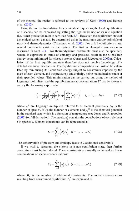
of the method, the reader is referred to the reviews of Keck (1990) and Beretta

et al. (2012).

Using the normal formulation for chemical rate equations, the local equilibration

of a species can be expressed by setting the right-hand side of its rate equation

(i.e. its net production rate) to zero (see Sect. 2.3). However, the equilibrium state of

a chemical system can also be determined using the maximum entropy principle of

statistical thermodynamics (Chiavazzo et al. 2007). For a full equilibrium state,

several constraints exist on the system. The first is element conservation as

discussed in Sect. 2.3. Two thermodynamic constraints must also be specified,

which, if expressed in terms of enthalpy and pressure, result in the Gibbs free

energy being minimised for closed systems (Jones and Rigopoulos 2005a). Calcu-

lation of the final equilibrium state therefore does not involve knowledge of a

detailed chemical mechanism. The equilibrium composition can instead be calcu-

lated by minimising its Gibbs free energy subject to constraints imposed by the

mass of each element, and the pressure p and enthalpy being maintained constant at

their specified values. This minimisation can be carried out using the method of

Lagrange multipliers, and the equilibrium molar concentrations Yj0 can be shown to

satisfy the following expression:

Y0j ¼

p

ρRT

�μ⦵j

RT

!exp

XMe

i¼1

aeijλ

ei

� �& ’j ¼ 1, . . .NSð Þ ð7:97Þ

where λie are Lagrange multipliers referred to as element potentials, NS is the

number of species, Me is the number of elements and μj⦵ is the chemical potential

in the standard state which is a function of temperature (see Jones and Rigopoulos

(2007) for full derivation). The matrix aeij contains the contributions of each element

i in species j. Element constraints can be represented as

Ei ¼XNj¼1

aeijYj

� �i ¼ 1, . . . ,Með Þ ð7:98Þ

The conservation of pressure and enthalpy leads to 2 additional constraints.

If we wish to represent the system in a non-equilibrium state, then further

constraints must be introduced. These constraints are usually expressed as linear

combinations of species concentrations:

Ci ¼XNS

j¼1

acijYj

� �i ¼ 1, . . . ,Mcð Þ ð7:99Þ

where Mc is the number of additional constraints. The molar concentrations

resulting from constrained equilibrium Yj* are expressed as




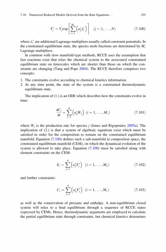
Y�j ¼ Y

0jexp

XMc

i¼1

acijλ

ci

� �& ’j ¼ 1, . . . ,Nð Þ ð7:100Þ

where λic are additional Lagrange multipliers usually called constraint potentials. In

the constrained equilibrium state, the species mole fractions are determined by Mc

Lagrange multipliers.

In common with slow manifold-type methods, RCCE uses the assumption that

fast reactions exist that relax the chemical system to the associated constrained

equilibrium state on timescales which are shorter than those on which the con-

straints are changing (Tang and Pope 2004). The RCCE therefore comprises two

concepts:

1. The constraints evolve according to chemical kinetics information.

2. At any time point, the state of the system is a constrained thermodynamic

equilibrium state.

The implication of (1.) is an ODE which describes how the constraints evolve in

time:

dCi

dt¼XNj¼1

acijWj

� �i ¼ 1, . . . ,Mcð Þ ð7:101Þ

where Wj is the production rate for species j (Jones and Rigopoulos 2005a). The

implication of (2.) is that a system of algebraic equations exist which must be

satisfied in order for the composition to remain on the constrained equilibrium

manifold. Equation (7.100) defines such a sub-manifold in composition space, the

constrained equilibrium manifold (CEM), on which the dynamical evolution of the

system is allowed to take place. Equation (7.100) must be satisfied along with

element constraints on the CEM:

Ei ¼XNj¼1

aeijY

�j

� �i ¼ 1, . . . ,Með Þ ð7:102Þ

and further constraints:

Ci ¼XNj¼1

acijY

�j

� �i ¼ 1, . . . ,Mcð Þ ð7:103Þ

as well as the conservation of pressure and enthalpy. A non-equilibrium closed

system will relax to a final equilibrium through a sequence of RCCE states

expressed by CEMs. Hence, thermodynamic arguments are employed to calculate

the partial equilibrium state through constraints, but chemical kinetics determines


the dynamic evolution of the system, i.e. how the constraints evolve in time,

through Eq. (7.101).

Equations (7.100–7.103) form a differential algebraic system of equations where

the number of constraints used determines the dimension of the reduced system.

Since the RCCE formulation leads to a general system of ODEs, it is also necessary

to select which variables the constraints should be applied to, since different

selections may lead to different model reduction errors. Most commonly, con-

straints are applied to individual species, but this may be more related to practical-

ities of implementation rather than inherent properties of the system. There is in

principle no reason why constraints should not be applied to combinations of

species (e.g. lumped variables). To summarise (Jones and Rigopoulos 2007), an

RCCE system comprises a set of ODEs or PDEs that describe the dynamics of the

kinetically controlled species taken directly from a detailed mechanism without any

approximations and a set of algebraic equations for the computation of the equil-

ibrated species, derived on a physical basis via the maximum entropy principle of

thermodynamics.

In Jones and Rigopoulos (2005a), RCCE was applied to the simulation of

methane laminar flames. The first two constraints chosen were necessarily CH4

and O2 since initial and boundary conditions must correspond to a constrained

equilibrium state for the set of constraints selected. Further constraints were then

tested on a trial-and-error basis until the reduced model with the lowest error

compared to the full model was obtained. Systems using 9 and 7 constraints were

tested and found to give good agreement with the full model containing 63 species.

The same set of constraints was also found to be satisfactory for the modelling of a

methane ignition problem. The RCCE method was also applied in Ugarte

et al. (2005) to a model of the combustion of a stoichiometric mixture of formal-

dehyde and oxygen which contained 29 species and 139 reactions over a wide range

of temperatures and pressures. Reduced models containing between 1 and 6 RCCE

constraints were tested along with three fixed element constraints (carbon, oxygen

and hydrogen). Overall eight constraints were needed to give good agreement with

ignition delays predicted by the full model, although slightly more were required

for the prediction of minor species.

The selection of constraint species by trial and error, however, could be time

consuming, and it would be useful to be able to automatically select the optimal set

of constraints which minimises the simulation error for a given reduced model

dimension. Hiremath et al. (2010, 2011) address this issue by developing a “greedy”

algorithm to select a “good” set of constrained species. Whilst this may not be the

globally optimal set, it is an improvement on trial-and-error approaches and was

demonstrated for a methane combustion model to produce the lowest reduction

error over a wide range of temperatures and pressures for partially stirred reactor

studies. The selection of constraints was also achieved using an LOI in Rigopoulos

and Løvas (2009) and more recently in Løvas et al. (2011), where the constraints

were selected adaptively in different regions of the composition space. Here a

cross-over between QSSA and RCCE methods occurs since the LOI is related to


the species lifetime (see Eqn (7.78)), and hence, the constrained species approxi-

mately correspond to non-QSS-species.

One advantage of RCCE is that it provides a consistent framework to derive

equations describing the reduced model based on the second law of thermo-

dynamics. This means that approaches such as tabulation or complex algebraic

manipulations based on the QSSA can be avoided. One drawback of the RCCE

approach, however, as pointed out by Tang and Pope (2004), is that the CEMs are

not inertial manifolds but only approximations to them. What this means is that the

RCCE manifolds produced are not the exact ones to which trajectories approach in

a simulation of the full system. However, the same could be said of the ILDM

formulation which also gives only an approximation to the exact inertial manifold.

For this reason, extensions to RCCE have been proposed (Ren et al. 2007) which

use CEMs as a starting point for trajectory-based methods which calculate the

corresponding inertial manifold (see later discussion in Sects. 7.11 and 7.12).

7.11 Numerical Reduced Models Based on Geometric

Approaches

7.11.1 Calculation of Slow Invariant Manifolds

As pointed out in the previous section, one potential disadvantage of ILDM and

RCCE methods is that they do not represent the exact invariant manifold of the

system but rather an approximation to it. The exact slow invariant manifold (SIM)

is that to which propagated trajectories are attracted, and once a trajectory has

reached an invariant manifold, it does not leave it (Gorban et al. 2004b). Singh

et al. (2002) demonstrate, for example, that an ILDM is not in general a SIM but

approaches one in the limit of large stiffness, i.e. clear timescale separation between

slow and fast dynamics. Several methods for determining such globally attracting

SIMs have been developed which fall into the class of geometric methods. Such

geometric methods include trajectory-based methods, iterative methods and the

invariant constrained equilibrium edge pre-image curve (ICE-PIC) method. Davis

and Skodje (1999) argue that geometric approaches are more general than other

approaches such as ILDM, since motion on a one-dimensional manifold need not

conform to a single exponential or a simple rate law except when close to the final

equilibrium point.

A full mathematical description of the definition of the invariance of an SIM is

given in Chiavazzo et al. (2007). Based on the concept of invariance, it follows that

the SIM can be obtained through the simulation of trajectories rather than via the

algebraic equations defined for the ILDM above. Hence, locating the invariant

manifold can be obtained by simulating the progress of reaction trajectories from

suitable initial conditions as they proceed towards equilibrium. Trajectory-based

methods for converging to the SIM using a predictor corrector algorithm were

7.11 Numerical Reduced Models Based on Geometric Approaches 257

discussed in Davis and Skodje (1999) with application to a hydrogen oxidation

mechanism. They demonstrated a higher degree of accuracy of the SIMs obtained

in this approach compared to QSSA- or ILDM-based reduction methods.

An alternative approach was also formulated by Fraser and co-workers (Fraser

1988; Roussel and Fraser 1990, 1991a, b, 2001; Fraser and Roussel 1994) who

suggested that the slow invariant manifold could be viewed as an attracting fixed

point of a functional mapping. Thus, an initial guess for the slow manifold

(e.g. based on the QSSA) could be iteratively improved. A method based on

functional equation truncation was also developed by Roussel and Tang (2006).

Davis and Skodje (1999) modified this method to allow its use for high-dimensional

systems. Both the trajectory-based approaches and an updated algorithm based on

Fraser’s original work were shown in their work to be more accurate than the ILDM

and QSSA for the test cases studied. A full discussion of the different approaches is

given in Skodje and Davis (2001).

A related approach termed the method of invariant grids (MIG) is also discussed

in Gorban and Karlin (2003), Gorban et al. (2004a, c), Chiavazzo et al. (2007, 2009)

based on the method of invariant manifold (MIM). In MIG, a quasi-equilibrium

approach is used to define a first approximation to the SIM on a grid in concen-

tration space, and then improved estimations of the SIM are obtained using either

Newton iteration or relaxation methods. The MIG was compared to CSP-based

methods, the ILDM method and the entropy-based methods in Chiavazzo

et al. (2007).

Singh et al. (2002) suggested a method where diffusion is taken into account

during the determination of the slow manifold. They called this manifold the

infinite-dimensional approximate slow invariant manifold (ASIM), and it is an

extension of the functional iteration techniques introduced by Roussel and

co-workers (Fraser 1988; Roussel and Fraser 1990, 1991a, b, 2001; Fraser and

Roussel 1994) discussed above. When applied to reactive flow systems, their

method results in an elliptic system of partial differential equations describing

motion on the infinite-dimensional ASIM which are obtained by equilibrating the

fast dynamics of the closely coupled reaction/convection/diffusion system. They

demonstrate the method for a model of ozone decomposition in a premixed laminar

flame and observe smaller errors in the simulation of key flame features than when

using the purely chemical ILDM. Similar approaches based on finding the ASIM

were also developed by Ren and Pope (2005, 2006b, 2007a, b) for

reaction�diffusion systems. A full discussion of the differences between the

ILDM, the close-parallel assumption and ASIM methods for reaction–diffusion

systems is given in Ren and Pope (2007b). The conclusion drawn is that whilst the

full ASIM approach gives accurate predictions of the full composition even close to

the solution boundaries, it is by far the most computationally expensive of the three

approaches. Ren and Pope (2007b) propose some simplifications to the general

approach adopted in Singh et al. (2002) in order to improve the efficiency of the

method based on the formulation of explicit governing PDEs for the reduced

composition (slow variables) rather than the full composition.


7.11.2 The Minimal Entropy Production Trajectory Method

A geometric-based method for the calculation of one-dimensional manifolds based

on thermodynamic principles was also developed, namely, the minimal entropyproduction trajectory (MEPT) method (Lebiedz 2004). This method can be inter-

preted as the demand that under the given constraints, all thermodynamic forces

and dynamic modes of the system remain maximally relaxed except one, the

progress variable, which is parameterised. This is equivalent to finding a trajectory

approaching equilibrium for which the squared deviation of the entropy production

from zero is minimal for a weighted sum of single reaction step contributions,

which is called the MEPT. The approach can be loosely linked with the application

of simple reduction rules such as partial equilibrium or quasi-equilibrium assump-

tions (see Sects. 2.3.2 and 2.3.4) since it can be interpreted as finding the model

configuration with as many elementary reaction steps as possible being close to

quasi-equilibrium in a chemical sense. Such a model is determined using an

optimisation algorithm.

These methods were further extended in Ugarte et al. (2005), Ren et al. (2007)

and Reonhardt et al. (2008) to two-dimensional manifolds which are computed as

families of MEPTs using a multiple shooting method with a range of initial values.

Hence, a discrete grid of initial values of the reaction progress variables is used, and

then optimal trajectories (based on the MEPT principle) are calculated which span

the two-dimensional manifold. However, Al-Khateeb et al. (2009), who investi-

gated the relationship between thermodynamics and a reactive system’s slow

invariant manifold, suggest that such a manifold cannot be a good representation

of the SIM. In their work they conclude that the MEPT is not attractive along its

complete trajectory, and thus does not correspond to the SIM of the system. A

mathematical analysis is provided which shows that equilibrium thermodynamic

potentials do not alone determine reactive systems’ dynamics during their approach

towards the physical equilibrium and are not attractive manifolds describing the

slow dynamics, even near the equilibrium point. It is worth noting the similarities

between the minimal entropy production trajectory (MEPT) method, the RCCE

(Sect. 7.10.4) and the entropy production-based skeletal mechanism reduction

method (Sect. 7.4).

7.11.3 Calculation of Temporal Concentration ChangesBased on the Self-Similarity of the ConcentrationCurves

Harstad and Bellan (2010a, b) investigated the concentration�time curves obtained

during the simulation of the ignition of large alkanes. They found that on plotting

the concentration of several species as a function of a selected dominant variable

(e.g. the normalised temperature), the resulting curves were similar to each other,

7.11 Numerical Reduced Models Based on Geometric Approaches 259



which means that one curve can be transformed to the other by a linear projection.

They distinguished local and global self-similarity; the former means that it occurs

only in some regions of the ( p0, T0, φ) space, whilst the latter is valid in the entire

investigated space. The concentrations of the large hydrocarbon intermediates were

calculated with the similarity equations, whilst those of the small radicals were

calculated using the QSSA approximation. This allowed them to create a reduced

model in which differential rate equations were solved for only 11 species. This

approach was used for formulating reduced models for the ignition of n-heptane(Harstad and Bellan 2010b) and various mixtures of iso-octane, n-heptane and n-pentane or iso-hexane (Harstad and Bellan 2010a) over a wide range of equivalenceratios, initial pressures and temperatures. The approach was developed further by

Kourdis and Bellan (Kourdis and Bellan 2014), who improved the numerical

methodology and extended it to further hydrocarbons.

Bellan et al. present the existence of self-similarity as an empirical observation

resulting from the inspection of simulation results, and they do not provide a

mathematical foundation to the method. Similar concentration curves may be a

result of the existence of very different timescales, and the application of QSSA or

partial equilibrium may result in linear relations between the concentrations.

However, in these articles self-similarity was found among long lifetime

(“heavy”) species, and therefore, the existence of self-similarity seems to be a

consequence of possible lumping relationships within the system variables.

Although the self-similarity concept seems to be related to the lumping of species,

it is not equivalent to it, since the derived linear functions contain the concentra-

tions of all heavy species and not only a selection of them.

7.12 Tabulation Approaches

In the previous two sections, several methods for model reduction were discussed

which in some way exploited the inherent low-dimensional manifolds that are

present in kinetic systems. In general, for high-dimensional nonlinear models,

such methods have to be applied numerically rather than by solving coupled set

of algebraic equations symbolically. Further speed-ups can be gained through the

use of storage and retrieval algorithms defining behaviour on the low-dimensional

manifolds. Within this class of methods, the simulations are usually carried out in

two steps. First, the system of equations is solved over many possible reaction

conditions, and the simulation results are stored using an appropriate information

storage and retrieval system. When further simulations are carried out at similar

conditions, the results can be deduced from the stored outputs.

Meisel and Collins were among the first authors who used this principle and

called it the repro-modelling approach. Meisel and Collins suggested that within a

large complex model, it is worth identifying very time-consuming subtasks which

are used frequently, where the results depend only on the values of a few variables

(Meisel and Collins 1973). It is immediately obvious that the presence of


low-dimensional manifolds in a system will lead to this type of behaviour. These

subtasks can be solved at many possible values of their variables, and the results are

fitted or stored as a function of a reduced number of variables (e.g. the

parameterising variables of the slow manifold). The fitted functions/tables can

then be used several thousand times during the simulation of the complex model,

and solutions are likely to be cheaper to retrieve, compared to the integration of a

stiff set of differential equations. Various strategies for storage and retrieval have

been developed which will be discussed in this and the following section. We start

here with tabulation methods.

7.12.1 The Use of Look-Up Tables

The relationship between the state of a model and the vector of chemical kinetic

information can be stored in tables. Such tables are called look-up tables in the

simulation of turbulent flames. When the simulation code receives the input vector,

it locates points within the table that are close to the input point within a high-

dimensional space. The output vector is composed using linear interpolation

between the output vector elements at the storage points.

During the creation of look-up tables, several aspects have to be taken into

account (Atanga 2012):

1. The information storage structure of the database must be optimised.

2. The CPU time needed to retrieve a stored value must be minimal.

3. The accuracy of the retrieved value has to meet specific criteria.

4. The required memory needed to store all the desired data must be affordable.

However, the search and retrieval algorithms required to access the look-up

tables can consume significant amounts of computational time. Special algorithms

have been developed to speed up the search and retrieval process (Androulakis

2004). The success of the methods is judged by their ability to give accurate

representations of the full kinetic system with the lowest computational calculation

and storage requirements. The time investment in generating the equivalent model

is also important for some applications, although for models used in repeated design

or operational control calculations this may be of lower priority.

Early applications of tabulation methods in turbulent combustion simulations

employed tabulations of large regions of the physically realisable composition or

thermochemical phase space. As a result, they tended to use highly reduced global

mechanisms in order to generate the look-up tables, in order to avoid the dimen-

sionality of the table becoming too large. In early implementations (Taing

et al. 1993; Chen et al. 1995), a regular mesh was used to cover the realisable

region of the composition space, with the reaction mapping determined by offline

integration of a highly reduced model for storage within the look-up table. In such

cases the success of the tabulated model is limited by the accuracy of the reduced

scheme employed to generate it. Examples include tabulations of a 3-step scheme

7.12 Tabulation Approaches 261

describing H2/CO combustion used in pdf calculations of turbulent non-premixed

flames in Taing et al. (1993) and the 1- and 2-step schemes describing the chemistry

of turbulent hydrogen jet flames in Chen et al. (1995). A similar methodology is the

flow-controlled chemistry tabulation (FCCT) method (Enjalbert et al. 2012). Using

this approach, the stored chemistry is based on the simulation results of partially

stirred reactors. For the simple reactor simulations, the mixing, the conditions of the

chemical reaction and the inflow/outflow were selected according to conditions

expected within the turbulent flame to be modelled.

An alternative, and potentially more accurate approach, would be to utilise the

concepts embodied in the low-dimensional manifold methods described in

Sect. 7.10 to identify a reduced number of variables for which the dynamics must

be described. A variety of methods can then be used to generate either tabulations or

training data, and a fitted algebraic model can be developed for the minimal number

of required variables. The advantage over the use of global mechanisms comprising

only a few steps is that full or skeleton chemical mechanisms could potentially be

used to generate the fitting data, bypassing the assumptions made in the generation

of global schemes. This is achievable since often homogeneous simulations can be

carried out using a detailed model, with the input–output relations of only a few key

variables used for tabulating the systems dynamics on the slow manifold which is

usually of a much lower dimension than the full composition space.

Tabulated chemistry was used in the simulation of cool flames (Colin

et al. 2005), which was based on the representation of ignition quantities such as

cool flame ignition delay, fuel consumption and reaction rates. The values used in

the tables were extracted from complex chemistry calculations for n-heptane. Theapproach was extended to the variable volume tabulated homogeneous chemistry(VVTHC) approach in Jay and Colin (2011). This approach provides the evolutionof major species and radicals from the onset of auto-ignition up to the end of the

expansion stroke for compression ignition and spark ignition engine applications. It

was first tested for homogeneous engine cases where it compared very well to

complex chemistry simulations. It was implemented in a piston engine combustion

model and used for the calculation of the burned gases volume variation behind a

propagating flame at constant pressure and in reproducing the subsequent compo-

sition evolution of kinetic differential equations. For this reason, tabulation

approaches are very often utilised within engineering simulations such as, for

example, engine piston simulations (Mosbach et al. 2008).

Tabulation was successfully used for the description of the oxidation of n-heptane, iso-octane, n-decane and n-dodecane. The agreement was good compared

with the results of detailed chemical calculations for all alkanes when only 20 pro-

gress variable light species were used (Kourdis and Bellan 2014). Tabulation was

applied by Xuan and Blanquart (2014) for the calculation of the concentrations of

polycyclic aromatic hydrocarbons (PAHs) in non-premixed flames.

A special utilisation of the tabulation of the final result of a combustion model

was incorporated into the NO relaxation approach (NORA) method in order to

predict thermal NO in combustion chambers (Vervisch et al. 2011). In the NORA

methodology, the NO reaction rate is written as a linear relaxation towards the


equilibrium value YeqNO with a characteristic time τ. Both parameters are tabulated as

functions of equivalence ratio, pressure, temperature and dilution mass fraction.

The table is generated on the basis of spatially homogeneous calculations but later

used within turbulent combustion models designed to simulate piston engine

applications. The approach has advantages for simulating NO emissions where

global kinetic models or tabulations have been used to simulate the turbulent fuel

combustion since sometimes radical concentrations may not be available for the

post combustion NOx simulations when using such approaches.

7.12.2 In Situ Tabulation

Early applications of tabulation methods in turbulent combustion simulations

employed tabulations of large regions of the physically realisable composition or

thermochemical phase space, thus necessitating the use of highly reduced global

mechanisms in the generation of the look-up tables. The use of full mechanisms

with potentially higher numbers of independent variables was limited in these early

applications by the storage requirements of the tabulation. This problem was

addressed in later developments of tabulation methods based on in situ tabulation

(Pope 1997), where only accessed regions of composition space are tabulated. This

allows higher-dimensional starting mechanisms to be used since these accessed

regions are substantially smaller than the physically realisable region in most

applications due to the presence of low-dimensional manifolds.

The first application of in situ adaptive tabulation (ISAT) was introduced by

Pope within a particle pdf (probability density function) model for turbulent

combustion (Pope 1997). Operator splitting is commonly used in the solution of

such systems so that the mixing and reaction terms are solved separately for a given

time step Δt (see Sect. 6.8). In practice the time step is chosen to be small in

comparison to the mixing timescale. Following the application of operator splitting,

it is possible to seek efficient methods for the solution of the purely chemical part of

the model equations, i.e. a reduced chemical model. As pointed out by Pope, in a

particle pdf model of turbulent combustion, solution of the chemical reaction term

may be required billions of times, which indicates the need for efficient compu-

tational methods. The same issue may also arise in Eulerian grid codes where

similar chemical compositions may be found within many grid cells during a full

reactive flow simulation (e.g. in atmospheric chemistry models). Both methods

suggest that during reactive flow calculations, regions of composition space may be

revisited many times, a feature which may be exploited in the development of

efficient solution methods.

The basic idea underpinning ISAT is the in situ tabulation of accessed regions of

composition space for a particular model application. The tabulation is achieved by

integrating the chemical source terms when a region is first accessed and then

storing the reaction mapping and sensitivity information in a binary tree data



structure. Subsequent estimations of the reaction mapping terms for points within a

small distance of the previously tabulated ones are achieved using multilinear

interpolation. Any reaction mapping that cannot be interpolated with sufficient

accuracy is generated by direct integration and added to the table. The method

therefore achieves the tabulation in situ rather than using offline calculations that

were employed within earlier tabulation approaches. It can be linked to the tabu-

lation of low-dimensional manifolds discussed in Sects. 7.10 and 7.11, since in

reality it is this manifold that will be accessed during the integration rather than the

full composition space. This allows significant reduction of the tabulation effort and

facilitates the use of detailed starting mechanisms that were not used within early

implementations of tabulation methods (Taing et al. 1993; Chen et al. 1995). Using

in situ methods, the accessed region is tabulated rather than the physically realisable

region. The presence of low-dimensional manifolds within the chemical system

ensures that the accessed region is usually much smaller than the realisable region.

The interpolation error that is incurred for accessed regions between mesh points

can be controlled by adaptive refinement of the mesh. The need for mesh refinement

is determined by establishing the region of accuracy for the tabulated points within

the mesh. This is defined as the connected region containing initial conditions

φ0 consisting of perturbed points φq for which the local error in the reaction

mapping terms ε does not exceed the specified tolerance εtol. In the ISAT method,

the region of accuracy is assumed to be a hyper-ellipsoid, which is related to the

mapping gradient matrix and the concentration sensitivities over the given time

step. The ISAT table consists of a binary tree: a set of records (one for each leaf of

the tree) and a set of cutting planes (one for each node of the tree) as shown in

Fig. 7.9.

Each record consists of the tabulation point (composition), the reaction mapping,

the mapping gradient matrix and the specification of an ellipsoid of accuracy within

which a linear approximation to the reaction mapping is valid. For each time step

during the calculation, a query is made for the given composition, and if the point

lies within the ellipsoid of accuracy (EOA) of a point within the table, then a linearapproximation to the mapping gradient is retrieved. Otherwise a direct integration

Fig. 7.9 A sketch of a

binary tree used within the

ISAT approach. At each

leaf (filled circle), there is arecord; at each node (emptycircle), there is information

about the cutting plane.

Reprinted from Pope (1997)

by permission of Taylor &

Francis Ltd, www.

tandfonline.com


http://www.tandfonline.com/

http://www.tandfonline.com/

of the reaction mapping is made and the actual error measured. If this error is less

than the specified tolerance for an already existing point, then the EOA for this

point is grown. Otherwise a new point is generated.

The approach was initially tested for methane�air combustion with 14 degrees

of freedom in a pairwise-mixing stirred reactor (Pope 1997). In this example the

control of local errors controls the global simulation errors well. The speed-up

factor of the method increases dramatically with the number of queries made to the

chemical source term, with speed-ups of up to 103 achieved for a large number of

queries. Cannon et al. (1999) compared the use of in situ methods to conventional

tabulation techniques for NOx predictions in CO combustion using a 5-step mech-

anism, showing that the storage requirements using the adaptive methods were up

to three orders of magnitude lower than conventional techniques due to the much

smaller size covered by the accessed region of composition space.

The ISAT method has been subsequently applied in a range of applications with

several additional developments to the methodology. In Yang and Pope (1998), a

method based on principal directions (ISATPD) was proposed in order to reduce the

dimensionality of the in situ tabulation. This method is based on the fact that, in the

principal directions of composition space, the trajectory of the composition point is

essentially restricted to a low-dimensional space, even though the original compo-

sition dimension may be very high. The data is therefore projected onto principal

directions (singular vectors) in order to improve the storage requirements leading to

more efficient search and retrieval algorithms. Androulakis (2004) demonstrated

the importance of the leading singular vectors for a range of mechanisms, illu-

strating that the number of leading eigenvectors is much smaller than the full

dimensionality of the problems studied. The use of the method by Yang and Pope

allowed skeletal mechanisms to be used for the tabulation rather than the global

schemes used in earlier applications of tabulation, thus improving the accuracy of

the reduced chemical model.

Further developments include the use of ISAT in a range of turbulent combus-

tion simulations. Pope and co-workers (Saxena and Pope 1999; Xu and Pope 2000;

Tang et al. 2000) have coupled the ISAT method with Monte Carlo joint pdfcalculations of turbulent reacting flows using an operator splitting approach,

allowing the representation of the finite rate kinetics necessary to capture important

features such as local flame extinctions and pollutant formation. Speed-ups of up to

a factor of 60 were reported in Saxena and Pope (1999) compared to conventional

chemistry calculations. Similar speed-ups were reported by Wang and Fox (2003)

in a pdf model for predicting reactive precipitation in time-evolving flows and Xie

et al. (2004) in a finite volume model of multi-phase fluidised beds. Higher speed-

ups (up to 165) have been reported for premixed combustors (James et al. 2001)

indicating that the accessed regions of composition space are smaller for premixed

flames compared to diffusion flames. A detailed analysis of speed-up factors and

possible improvements to the search and retrieval algorithms based on binarysearch trees (BSTs) was given by Chen (2004). The method suggested was based

on ensuring that the table entry closest to the inquiry point is retrieved, which

potentially increases the number of retrieval operations compared to directly


integrated steps. This is achieved by conducting a reverse traversal of the binary

tree structure when a retrieval fails, in order to find a table entry closer to the

inquiry. Speed-ups of up to a factor of 5 compared to conventional BSTs were

reported.

A detailed error analysis of ISAT was performed in Saxena and Pope (1999) for

a pairwise-mixing stirred reactor (PMSR) utilising a reduced 16 species scheme for

methane combustion. The analysis showed a straightforward relationship between

local interpolation errors and global errors for this case study. Slightly larger

relative global errors were incurred for the minor species compared to the major

ones. The conclusion of the work was that the global accuracy can be adequately

controlled for species of interest by suitably choosing a local error tolerance. Liu

and Pope (2005) performed further detailed error analysis of ISAT for turbulent pdfcalculations of a piloted jet methane/air flame using a skeleton methane mecha-

nism. They discussed various methods for growing EOAs with the standard ellip-

soid method giving similar results compared to more conservative methods such as

conical growing. They also discussed possible sources of the large local errors that

occasionally occur during retrieval, citing non-convex regions of accuracy as the

main reason. Again for this example, the global errors are reported to scale linearly

with respect to local errors. Improvements in the search strategies and error

correction algorithms were also suggested in Lu and Pope (2009).

A range of other applications of ISAT to combustion-related problems exist in

the literature. ISAT has also been employed using the Strang operator splitting

methods (Strang 1968) for reaction–diffusion systems (Singer and Pope 2004;

Singer et al. 2006) and for unsteady reacting flows in one and two dimensions

with relevance to potential application in direct numerical simulation (DNS) codes.

Masri et al. (2004) incorporated the ISAT technique into the commercial CFD code

FLUENT using a hybrid Reynolds-averaged Navier–Stokes (RANS) pdf approachwith application to flame lift-off. Their work demonstrated the ability of ISAT to

represent chemistry with sufficient detail to model auto-ignition phenomena within

turbulent jets of H2/N2 mixtures into co-flows of hot gas mixtures. Engine simu-

lations using ISAT were performed in Contino et al. (2011). Mazumder (2005)

adapted the ISAT technique to heterogeneous surface reactions with application to

the catalytic combustion of a methane–hydrogen mixture on platinum using a

19-species reaction mechanism. The heterogeneous part of the problem was differ-

ent from the solution of gas-phase chemistry since it required the solution of

nonlinear algebraic equations instead of a standard initial value problem. In this

case the use of operator splitting was prohibited due to the fact that the surface

processes were kinetically rather than diffusion limited. Transport and surface

chemistry therefore needed to be solved together, leading to coupled nonlinear

algebraic relationships. However, since ISAT can generally be used to map input–

output relationships, the technique was easily adapted by Mazumder to represent

the relationship between input parameters and predicted outputs of the resulting set

of coupled nonlinear equations. In this case the inputs were the diffusion velocities

and concentrations of the gas-phase species and the wall temperature, and the

outputs the wall concentrations of all the species. ISAT was also applied to the


catalytic combustion of methane on a platinum surface in Kumar and Mazumder

(2011), this time using an unstructured CFD approach. Cunha and da Silva (2014)

also tested the ISAT method, focusing on the issues of accuracy, efficiency and

memory usage in the simulation of homogeneous stirred reactor models using the

GRI 3.0 methane combustion mechanism. They found that the ISAT implemen-

tation had an absolute global error smaller than 1 %, whilst 34 % of the compu-

tational time was saved.

More recent applications of ISAT type methods have been coupled to the types

of dimension reduction techniques described in previous sections in order to exploit

the existence of low-dimensional manifolds in composition space. The use of in situ

tabulation then equates to the tabulation of reaction mappings for the reduced

variables within accessed regions of the low-dimensional manifold, rather than

the tabulation of the whole realisable region of the manifold. To a certain extent, the

issue of dimensionality was addressed in the ISATPD method, although in this case

the reduced representation was in the singular vector space rather than the original

composition or thermochemical space. More recent methods address the adaptive

tabulation of low-dimensional manifolds in the original thermochemical space.

Tang and Pope (2002) developed a method for the tabulation of rate-controlled

constrained equilibrium (RCCE) manifolds as discussed in Sect. 7.10.4. This

allowed detailed rather than reduced kinetic schemes to be used for the in situ

tabulation, since the table is generated for only a small number of constraints or

constraint potentials necessary to describe the chemical system. The method was

tested for the comprehensive methane scheme GRIMech 1.2 (32 variables) using

16 constraint potentials, with the results compared against the tabulation of a

17-variable mechanism reduced by conventional techniques including the QSSA.

The relative accuracy of the two methods depends on the assumptions made with

the conventional mechanism reduction compared to those made in the constrained

equilibrium approach, with comparable results achieved in the pairwise-mixing

stirred reactor case studied by Tang and Pope.

7.12.3 Controlling Errors and the Invariant ConstrainedEquilibrium Pre-image Curve (ICE-PIC) Method

An extremely important issue with regard to all tabulation or fitting methods is that

the global errors should not grow beyond an acceptable level during a time-

dependent simulation. Since most of the methods described in this and the next

section are based on controlling the local fitting error, it follows that the relationship

between local and global errors is important. In applications which tend towards an

equilibrium point, one would expect this relationship to be favourable since reac-

tion trajectories tend to converge, at least within a region of the equilibrium point

which may be quite large. The discussion of the ISAT method above indicated that

for most applications tested, the global modelling error scaled linearly with the


overall tolerance chosen for the ellipsoid of accuracy. However, for systems

exhibiting complex dynamics such as oscillatory or even chaotic behaviour, the

relationship between local and global errors may be more complex. Brad

et al. (2007) demonstrated that for CO/H2 combustion in a continuously stirred

tank reactor (i.e. an open system), trajectories could diverge substantially over short

time intervals during the early stages of ignition, indicating that the local fitting

error had to be more tightly controlled within these low-temperature regions in

order to control the overall modelling error. It may follow therefore that controlling

the local error using the same tolerance in all regions of thermochemical space is

not optimal, since in higher-temperature regions where nearby trajectories rapidly

converge, larger local errors may be tolerated.

Ensuring mass conservation has been reported to be an important feature of

controlling the global error (Tonse et al. 1999; Brad et al. 2007) when using

tabulation/fitting methods. In the context of the use of low-dimensional manifolds,

this involves modelling not only the key variables but also the other variables

(which are usually fast variables) in order to reconstruct the whole composition

space. Several methods can be used to generate concentrations of the fast variables.

If available, algebraic expressions based on the QSSA can be employed. Where

such expressions are highly coupled, then alternative approaches have been

suggested based on ILDM tabulations, RCCE and local repro-models. The recon-

struction of these species should however be achieved locally within the context of

operator splitting, without the need for them to be included in complex flow

calculations.

An alternative method for species reconstruction based on pre-image curves was

developed by Ren and Pope within the invariant constrained equilibrium edge

pre-image curve (ICE-PIC) method (Ren and Pope 2005; Ren et al. 2006; Pope

and Ren 2009). This is a trajectory-based method, where a very good approxima-

tion to the invariant manifold is determined by computing trajectories of the full

system from appropriate initial conditions. The method can be applied to local

reconstruction of species on, or close to, the inertial manifold, since the local initial

conditions of the trajectories are defined using a pre-image curve. The method is

local in nature and therefore may be more computationally efficient than the global

methods used to determine SIMs such as those based on trajectory or functional

iteration methods (see Sect. 7.11.1). Al-Khateeb et al. (2009), however, compared

SIMs with ICE-PIC-generated manifolds for a simple hydrogen–oxygen reactive

system, and showed that the ICE-PIC-generated manifold did not contain the SIM

over its whole range and that the error of the ICE-PIC manifold grew away from the

equilibrium point of the system. Nevertheless, since the ICE-PIC method uses

trajectories, it provides a closer approximation to the SIM than RCCE methods.

The pre-image curve provides the initial conditions for trajectory simulations

and is not necessarily unique, as initial points from a sizeable region of the

pre-image manifold will give rise to reaction trajectories that end up on or very

close to the SIM if the manifold is strongly attractive (Ren and Pope 2005). This is

illustrated in Fig. 7.10 where many trajectories are seen to end up close to the point

A which lies on the SIM. For a given composition of the reduced variables, the


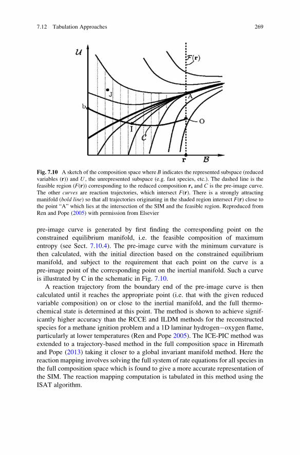
pre-image curve is generated by first finding the corresponding point on the

constrained equilibrium manifold, i.e. the feasible composition of maximum

entropy (see Sect. 7.10.4). The pre-image curve with the minimum curvature is

then calculated, with the initial direction based on the constrained equilibrium

manifold, and subject to the requirement that each point on the curve is a

pre-image point of the corresponding point on the inertial manifold. Such a curve

is illustrated by C in the schematic in Fig. 7.10.

A reaction trajectory from the boundary end of the pre-image curve is then

calculated until it reaches the appropriate point (i.e. that with the given reduced

variable composition) on or close to the inertial manifold, and the full thermo-

chemical state is determined at this point. The method is shown to achieve signif-

icantly higher accuracy than the RCCE and ILDM methods for the reconstructed

species for a methane ignition problem and a 1D laminar hydrogen�oxygen flame,

particularly at lower temperatures (Ren and Pope 2005). The ICE-PIC method was

extended to a trajectory-based method in the full composition space in Hiremath

and Pope (2013) taking it closer to a global invariant manifold method. Here the

reaction mapping involves solving the full system of rate equations for all species in

the full composition space which is found to give a more accurate representation of

the SIM. The reaction mapping computation is tabulated in this method using the

ISAT algorithm.

Fig. 7.10 A sketch of the composition space where B indicates the represented subspace (reduced

variables (r)) and U , the unrepresented subspace (e.g. fast species, etc.). The dashed line is the

feasible region (F(r)) corresponding to the reduced composition r, and C is the pre-image curve.

The other curves are reaction trajectories, which intersect F(r). There is a strongly attracting

manifold (bold line) so that all trajectories originating in the shaded region intersect F(r) close tothe point “A” which lies at the intersection of the SIM and the feasible region. Reproduced from

Ren and Pope (2005) with permission from Elsevier


7.12.4 Flamelet-Generated Manifolds

The above approaches to tabulation, whilst mostly applied in the simulation of

combustion problems, have a general foundation that would be relevant to many

kinetic systems. However, a special class of tabulation methods has been developed

for flame simulations. If a fast exothermic reaction takes place between two

components (e.g. a fuel and an oxidiser) of a gaseous system, then flames are

observed. In premixed flames the fuel and the oxidiser are premixed before com-

bustion takes place, whilst in non-premixed (diffusion) flames, the fuel and the

oxidiser diffuse into each other, and the flame occurs at the boundary or flame front.

Premixed and non-premixed flames are two extreme cases, but in many practical

flames, continuous states between these two extremes will exist. Flames can be

classified as laminar or turbulent according to the characteristics of the flow. Flames

are special types of reaction�diffusion systems, characterised by high spatial

gradients in temperature and species concentrations, and consequently reaction

rates will have a high spatial variability.

Often, for the purposes of simplifying the modelling task, the edge of a turbulent

flame is approximated by an ensemble of discrete, steady laminar flames, called

flamelets (Libby and Bray 1980; Liew et al. 1981). The individual flamelets are

assumed to have a similar structure to laminar flames for the same concentration

and temperature conditions so that detailed calculations of the flamelet chemistry

can be obtained from lower-dimensional numerical calculations. Laminar opposed-

flow diffusion flamelets for non-premixed combustion can then be embedded

within a turbulent flame, for example, using statistical pdf methods. This approach

is adopted in the description of the chemical processes in flames through flamelet-generated manifolds (FGM) (van Oijen et al. 2001), also known as flame-prolongated ILDMs (FPI) (Gicquel et al. 2000; Pera et al. 2009). In these methods,

spatially one-dimensional, premixed and non-premixed flames are first simulated

using a detailed reaction mechanism. Counter-flow diffusion flame simulations are

often used for this purpose (Verhoeven et al. 2012).

The flamelets are usually computationally cheap to produce, even using detailed

mechanisms containing several hundred reaction steps, since they are based on

one-dimensional simulations. These simulations can therefore be performed over a

wide range of conditions, e.g. using a large number of boundary conditions,

pressures and temperatures, so that the simulations cover the expected conditions

within the three-dimensional turbulent flames of interest. The results of the calcu-

lations are stored in databases, and these empirical manifolds are used for the

simulation of two- and three-dimensional flames, when direct simulation would

require far more computational time. For the simulation of two- and three-

dimensional turbulent flames, the values of only a few variables are usually

calculated such as the local enthalpy and conversion. It is then assumed that the

local structure of a flame having complex geometry is similar to those of a

one-dimensional flame, and the concentrations of the calculated variables are

obtained from the database. A number of applications of flamelet-generated


manifolds have been published, and the accuracy of this approximation was inves-

tigated over various conditions for modelling the combustion of fuels such as

hydrogen, methane (Bilger 1990; Gicquel et al. 2000, 2006; van Oijen and de

Goey 2000, 2002; van Oijen et al. 2001; de Goey et al. 2003; Bongers

et al. 2005; Fiorina et al. 2005; Godel et al. 2009; Verhoeven et al. 2012), benzene

(Xuan and Blanquart 2014) and even diesel oil (Bekdemir et al. 2011). In another

approach (Michel et al. 2008, 2009, 2010), flamelet-like libraries were generated

based on perfectly stirred reactor (PSR) calculations in terms of auto-ignition

delays and steady-state profiles of the progress variable. Lamouroux et al. (2014)

stored flamelets using the tabulated chemistry approach. The chemical information

is then applied in a turbulent combustion model within the large eddy simulation

(LES) framework. The use of in situ flamelet-generated manifolds was suggested in

Lodier et al. (2011). A procedure for building converged composition space solu-

tions for premixed flamelets was proposed and tested. This method provides the

framework for an efficient in situ calculation of complex chemistry with differential

diffusion to be applied to three-dimensional unsteady flame simulations.

7.13 Numerical Reduced Models Based on Fitting

Although sophisticated methods for the storage and retrieval of tabulated data have

been developed, there is still a computational overhead in using these techniques.

An alternative approach to storage and retrieval is the use of functional represen-

tations of the time-dependent kinetic changes or the look-up table contents, using,

for example, polynomial functions or artificial neural networks. In such represen-

tations, only the coefficients of the functions need be stored rather than the data

itself, and hence, the memory requirements and computational costs of evaluating

the fitted functions should be lower than for standard tabulation methods. However,

the overall accuracy of the operational model will depend on achieving high

accuracy of the fits across the model domain. This repro-modelling principle can

be used for the development of general algorithms for performing fast kinetic

simulations (Turanyi 1994, 1995). If a detailed mechanism has been reduced to a

skeletal mechanism, its differential (or algebraic-differential) equation can be

transformed to a difference equation that can be evaluated very quickly. One

disadvantage of these methods is that unlike tabulations, they are not guaranteed

to be completely accurate everywhere and should not be extrapolated beyond the

conditions under which the functional fits were obtained. They have, however, been

successfully applied within repro-modelling approaches for kinetic models, and

several of the most widely used methods will therefore be discussed here.

7.13 Numerical Reduced Models Based on Fitting 271

7.13.1 Calculation of Temporal Concentration ChangesUsing Difference Equations

The characteristic timescale of a system is the time period during which the events

occur that are of interest to us. For the simulation of the same physical system,

several different timescales can be selected according to the purpose of the model-

ling. The requirement is that during this period all interesting changes should be

completed. A mathematical model of a particular phenomenon should represent the

changes to its important features over the characteristic timescale. In the case of

kinetics, this may include changes in species concentrations or temperature. Usu-

ally these changes are simulated by integrating the kinetic differential equations for

the system, but the changes can also be stored and re-accessed.

One possible approach for storing the solution of a kinetic model is according to

the following general algorithm:

1. Time step Δt is selected to achieve good resolution of the characteristic time-

scale of the system.

2. Several thousand, spatially homogeneous simulations are carried out with a

series of initial concentrations and/or temperatures, which are typical for the

circumstances of applications of the final intended model.

3. The Y(t), Y(t+Δt) concentration vector pairs are stored in a database.

4. A function G is fitted to the data and can then be used to predict the change in

concentration after time step Δt : Y(t+Δt)¼G(Y(t)).

In spatially homogeneous simulations, the concentration�time curves (with

resolution Δt) can be obtained via a recursive evaluation of function G. If operator

splitting is used in a reactive flow model (i.e. the solution of the flow and chemistry

steps are separated), then this fitted function can be applied instead of typically

using implicit integration methods to solve the chemical rate equations. Potentially

large savings in computational effort can be achieved.

This method was called the repro-modelling approach in Dunker (1986) and

Turanyi (1994). The applicability of repro-modelling depends on the determination

of function G. This function converts n old concentrations to n new concentrations

and thus is an ℜn!ℜn mapping. However, it may be equally good to develop

piecewise fits using n pieces of ℜn!ℜ functions. In order to be successful, the

fitted function has to give an accurate approximation within the domain of appli-

cability for the final intended model. The selection of the initial simulation condi-

tions is therefore critical, since often, fitted functions may exhibit odd behaviour if

utilised outside of the original fitting domain. The function should also be quick to

evaluate, and several possibilities exist for suitable functional representations of

G as discussed later.

An early application of this idea was used by Dunker (1986), who applied it to

the modelling of tropospheric ozone formation. He started from a lumped mecha-

nism containing 47 species and identified 10 parameterising variables (species

concentrations or functions of species concentrations). All in all, 20,736 grid points


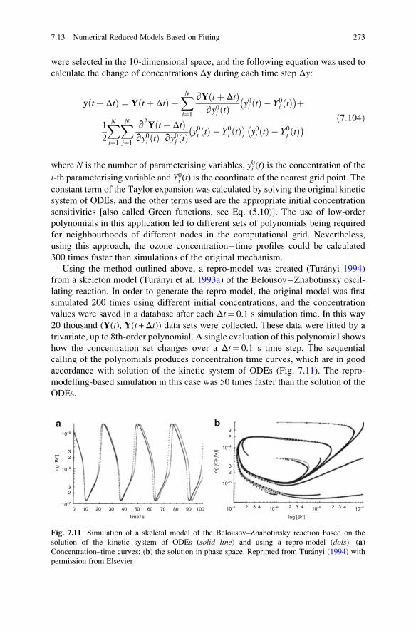
were selected in the 10-dimensional space, and the following equation was used to

calculate the change of concentrations Δy during each time step Δy:

y tþ Δtð Þ ¼ Y tþ Δtð Þ þXNi¼1

∂Y tþ Δtð Þ∂y0i tð Þ y0i tð Þ � Y0

i tð Þ� �þ1

2

XNi¼1

XNj¼1

∂2Y tþ Δtð Þ

∂y0i tð Þ ∂y0j tð Þ y0i tð Þ � Y0i tð Þ� ��

y0j tð Þ � Y0j tð Þ� ð7:104Þ

where N is the number of parameterising variables, y0i (t) is the concentration of the

i-th parameterising variable and Y0i (t) is the coordinate of the nearest grid point. Theconstant term of the Taylor expansion was calculated by solving the original kinetic

system of ODEs, and the other terms used are the appropriate initial concentration

sensitivities [also called Green functions, see Eq. (5.10)]. The use of low-order

polynomials in this application led to different sets of polynomials being required

for neighbourhoods of different nodes in the computational grid. Nevertheless,

using this approach, the ozone concentration�time profiles could be calculated

300 times faster than simulations of the original mechanism.

Using the method outlined above, a repro-model was created (Turanyi 1994)

from a skeleton model (Turanyi et al. 1993a) of the Belousov�Zhabotinsky oscil-

lating reaction. In order to generate the repro-model, the original model was first

simulated 200 times using different initial concentrations, and the concentration

values were saved in a database after each Δt¼ 0.1 s simulation time. In this way

20 thousand (Y(t), Y(t+Δt)) data sets were collected. These data were fitted by a

trivariate, up to 8th-order polynomial. A single evaluation of this polynomial shows

how the concentration set changes over a Δt¼ 0.1 s time step. The sequential

calling of the polynomials produces concentration time curves, which are in good

accordance with solution of the kinetic system of ODEs (Fig. 7.11). The repro-

modelling-based simulation in this case was 50 times faster than the solution of the

ODEs.

10–5

10–6

10–7

10–4

10–5

10–7 10–6 10–5

23

a b

32

log

[Br– ]

log

[Ce(

IV)]

time / s

0 10 20 30 40 50 60 70 80 90 100

32

32

3 42 3 42

log [Br–]

10–43 42

Fig. 7.11 Simulation of a skeletal model of the Belousov–Zhabotinsky reaction based on the

solution of the kinetic system of ODEs (solid line) and using a repro-model (dots). (a)

Concentration–time curves; (b) the solution in phase space. Reprinted from Turanyi (1994) with



7.13.2 Calculation of Concentration Changes by Assumingthe Presence of Slow Manifolds

An alternative to using in situ tabulation as discussed above was to tabulate the

systems dynamics on the slow manifold which is usually of a much lower dimen-

sion than the full composition space. A related approach is the parameterisation of a

tabulated ILDM as discussed in this section or the fitting of dynamics on

low-dimensional invariant manifolds using trajectory-generated data, i.e. on an

SIM (Lowe and Tomlin 2000a, b; Skodje and Davis 2001; Buki et al. 2002; Brad

et al. 2007). Ideally it would be useful to evaluate the minimum number of variables

required to accurately describe the dynamics within the manifold a priori, so that

different dimensions do not have to be tested. A number of studies of chemical

reaction systems have been carried out using timescale analysis along trajectories in

order to determine the intrinsic dimension of the slow manifolds (Tomlin

et al. 2001; Buki et al. 2002; Zsely et al. 2005; Ren and Pope 2006a; Brad

et al. 2007; Davis and Tomlin 2008a, b). A method for the determination of the

dimension of the manifold was introduced in Sect. 6.5. This dimension can be

surprisingly low (1�3) for models such as those describing the high-temperature

combustion of fuels such as hydrogen (Buki et al. 2002; Ren and Pope 2006a), wet

carbon monoxide (Brad et al. 2007) and hydrocarbons (Ren and Pope 2006a). The

fitted difference equations can therefore be of low dimension.

Yang et al. (2013) discussed the various ways for the determination of manifolds

from simulation data; they call the manifolds identified this way the empirical low-dimensional manifolds (ELDMs). The simplest ELDM is the plane manifold

obtained from the principal component analysis (PCA) (Sutherland and Parente

2009; Parente et al. 2009, 2011; Bilgari and Sutherland 2012; Coussement

et al. 2012, 2013; Mirgolbabaei and Echekki 2013, 2014; Mirgolbabaei

et al. 2014). A correlation analysis of two-dimensional direct numerical simulation

(DNS) data of a turbulent non-premixed H2/air flame with detailed chemistry was

used to find the ELDMs (Maas and Thevenin 1998). Proper orthogonal decompo-

sition (POD) analysis has also been applied to obtain low-dimensional represen-

tations of DNS data for H2/air flames (Frouzakis et al. 2000; Danby and Echekki

2006) and to simplify an atmospheric chemistry mechanism (Sportisse and Djouad

2000). Yang et al. (2013) applied both PCA and multivariate adaptive spline

regression (MARS) to DNS databases of a non-premixed CO/H2 temporally evolv-

ing jet flame and of an ethylene lifted jet flame.

In such methods a suitable data set for fitting the low-dimensional surrogate

model is generated over a wide range of temperatures, pressures and mixture

compositions, by integrating the system of differential equations from a variety of

initial conditions chosen to include all behavioural properties of the system. Once

the trajectories have settled onto the lower-dimensional manifold, the concen-

trations are stored and can be fitted using the repro-modelling approach (Turanyi

1995; Lowe and Tomlin 2000a, b; Buki et al. 2002). The collected data can also be

used to determine the maximum dimension of the slow manifold Nz (see Sect. 6.5).




The recommended algorithm is similar to the previous one:

1. Time step Δt is selected to achieve good resolution of the characteristic time-

scale of the system.

2. Several thousand, spatially homogeneous simulations are carried out with a

series of initial concentrations and/or temperatures, which are typical for the

circumstances of applications of the final intended model.

3. The Y(t), Y(t+Δt) concentration vector pairs are stored in a database.

4. An analysis of the data (e.g. using methods outlined in Sect. 6.5) leads to the

determination of highest dynamical dimension NZ.

5. Some variables of the model (e.g. concentrations) are selected as the

parameterising variables. These variables are denoted as α1, α2, . . . , αNZ.

6. Function G1 is fitted to the data and can then be used to predict the change in

parameterising variables after time step Δt : α(t+Δt)¼G1(α(t)).7. The same set of recorded concentrations is used to obtain fitted function G2 that

relates all concentrations to the parameterising variables: Y¼G2(α). This G2

function is similar to function that was introduced at the beginning of Sect. 7.10.

Functions G1 and G2 can be any appropriate mathematical function, and a

variety of possible choices is discussed below. In spatially homogeneous simu-

lations, the time dependence of the NZ parameterising variables can be obtained via

the sequential calling of function G1, whilst the values of all variables (concen-

trations) can be reconstructed using function G2. In spatially inhomogeneous

calculations using operator splitting (see Sect. 6.8), functions G1 and G2 are part

of the chemical term.

7.13.3 Fitting Polynomials Using Factorial Design

The use of polynomial fits is a possible alternative to the application of tabulations.

If the values of the input variable vector are assumed to be independent from each

other, then for each variable a minimum xmini and maximum xmax

i value can be

defined. The (xmini , xmax

i ) sets for all variables define a hyper-rectangle in the space

of input variables. This is also called the full factorial design arrangement of the

variable values (Box et al. 1978). Frenklach et al. (1992) suggested the creation of

fitted second-order polynomials for the construction of surrogate models where the

variable vectors used as the independent variables of the fitting were arranged

according to a full factorial design. In this way all possible variable value combi-

nations were well represented. This method has been shown to provide reliable and

accurate response surfaces. However, its application may become computationally

expensive when the number of variables is large. Surrogate models based on

factorial design have been and are routinely used in model optimisation studies

by Frenklach et al. (Frenklach et al. 2004; Feeley et al. 2004, 2006; Russi

et al. 2008, 2010; You et al. 2011, 2012). In the field of model reduction, Marsden




et al. (1987) suggested a similar method for the creation of a repro-model for ozone

production in the troposphere using a 15-variate polynomial which was fitted to a

series of simulations, arranged according to a factorial design.

7.13.4 Fitting Polynomials Using Taylor Expansions

A kind of cross-over between tabulation and polynomial storage methods is the

application of a collection of Taylor expansions. The exact values are tabulated at

some fixed points x of the input vector, but the values in between the tabulated

points are determined not by linear interpolation but according to the following

Taylor expansion:

Yi xþ Δxð Þ ¼ Yi xð Þ þXmj¼1

∂Yi

∂xjΔxj þ 1

2

Xmk¼1

Xmj¼1

∂2Yi

∂xk∂xjΔxkΔxj þ . . . ð7:105Þ

Here Yi(x) is the stored exact value,Δx is the deviation of the queried point from the

stored point, and ∂Yi/∂xj and ∂2Yi/∂xk∂xj are the first-order and second-order local

sensitivity coefficients, respectively. There are several efficient numerical methods

for the calculation of the first-order local sensitivity coefficients (see Sect. 5.2). The

second-order local sensitivity coefficients can be calculated from the first-order

coefficients using a finite-difference approximation. The Taylor series approxi-

mations have the general disadvantage that the accuracy significantly decreases

further from the central point.

Davis et al. proposed the application of a Taylor expansion for constructing

kinetic response surfaces used in the development and optimisation of reaction

kinetic models (Davis et al. 2004). They termed it the sensitivity analysis-based

(SAB) method. Tests indicated that for gas-phase combustion models, the response

surface obtained with the SAB method was as accurate as the factorial design

method previously used in reaction model optimisation, but using the sensitivity

coefficients calculated by the combustion simulation codes allowed significant

computational savings. This method was used in all later mechanism optimisation

studies by Wang et al. and Sheen et al. (Davis et al. 2004; Sheen et al. 2009, 2013;

Sheen and Wang 2011a, b).

7.13.5 Orthonormal Polynomial Fitting Methods

The previous two polynomial fitting methods resulted in second-order polynomials.

In some applications, however, second-order approximations are not accurate

enough, and higher-order polynomials have to be applied. Since general high-

order polynomials will have a large number of coefficients, it follows that the



approach becomes feasible only if a large number of these can be set to zero.

Methods for the determination of the coefficients of high-order polynomials have to

be suitable for fitting a polynomial function to tens of thousands of data points and

determining coefficients for the effective variables only, usually using a least-

squares-based method. The application of orthonormal polynomials (Turanyi

1994) can be advantageous for this task, since their coefficients can be determined

independently from each other. A method for fitting multivariate orthonormal

polynomials for many data points is therefore outlined below.

We first denote xi¼ (xi1, xi2, . . ., x

im), i¼ 1, . . ., n to be a data set and φj, j¼ 1,. . .,l

to be a set ofℜm!ℜ functions with appropriate weights wi, i¼ 1,. . .,n. The scalarproduct of functions φj and φk can be interpreted in the following way:

φj;φk

� � ¼Xni¼1

wiφj xi

� �φk xi� � ð7:106Þ

This means that the scalar product is determined not only by functions φj and φk

but also the data set and the values of weights wi. Functions φj and φk are

orthonormal with respect to scalar product (7.106), if

φj;φk

� � ¼ 0 if j 6¼ k1 if j ¼ k

�ð7:107Þ

Any function F: ℜm!ℜ can be approximated using the set of orthonormal

functions φj, j¼ 1,. . .,l by a Fourier expansion:

F �Xlj¼1

F;φj

� �φj ð7:108Þ

The deviation between function F obtained from the full model and its approxi-

mation can be characterised by the error r:

r ¼ F�Xlj¼1

F;φj

� �φj

�� ð7:109Þ

where kk denotes the Euclidean norm. This error is also called the root mean square

(r.m.s.) error. For each l� n, the approximation in Eq. (7.108) is the best, according

to the following relationship

r � F�Xlj¼1

ajφj

�� ð7:110Þ

where coefficients aj, j¼ 1,. . .,l are arbitrary real numbers.


The application of Fourier expansion (7.108) requires orthonormal functions,

which can be generated from independent functions using the Gram�Schmidt

orthonormalisation process. We denote fj, j¼ 1,. . ., l to be a set of linearly inde-

pendent functions. Using these functions, orthonormal functions can be generated

as follows:

φ1 ¼ c11 f 1φ2 ¼ c21 f 1 þ c22 f 2φ3 ¼ c31 f 1 þ c32 f 2 þ c33 f 3⋮

φl ¼Xlj¼1

cljf j

ð7:111Þ

Coefficients c are calculated using the equations below according to the

Gram�Schmidt process:

φ01 ¼ f 1 φ1 ¼ φ

01= φ

01

�� φ

02 ¼ f 2 � φ1; f 2ð Þφ1 φ2 ¼ φ

02= φ

02

�� ⋮

φ0l ¼ f l �

Xl�1

j¼1

φj; f l� �

φj φl ¼ φ0l= φ

0l

�� c11 ¼ 1= φ

01

�� c21 ¼ � φ1; f 2ð Þc11= φ

02

�� c22 ¼ 1= φ

02

�� clk ¼ �

Xl�1

j¼1

φj; f l� �

cjk

" #= φ

0l

�� k 6¼ l

cll ¼ 1= φ0l

��

ð7:112Þ

A possible set of linearly independent functions are the monomials of a poly-

nomial. For example, the monomials of a trivariate, second-order polynomial are

the following: 1, x, y, z, x2, xy, xz, y2, zy and z2. The general form of the monomials

is given by

Mj ¼Ymk¼1

xμ kj

k , μ kj 2 0, 1, 2, . . . , lf g ð7:113Þ

The order of the monomial isXmk¼1

μ kj , whilst the order of the polynomial is equal to

the highest-order monomial within the polynomial.

In reaction kinetics simulations, we might wish that the relative accuracy of the

fitted concentrations should be equal for both low and high concentrations

(e.g. radicals and products). For this reason, a weighting function wi¼ 1/F2(xi) is


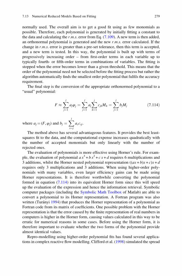
normally used. The overall aim is to get a good fit using as few monomials as

possible. Therefore, each polynomial is generated by initially fitting a constant to

the data and calculating the r.m.s. error from Eq. (7.109). A new term is then added,

an orthonormal polynomial is generated and the new r.m.s. error calculated. If thechange in r.m.s. error is greater than a pre-set tolerance, then this term is accepted,

and a new term is tested. In this way, the polynomial is built up with terms of

progressively increasing order – from first-order terms in each variable up to

typically fourth- or fifth-order terms in combinations of variables. The fitting is

stopped when the error becomes lower than a given threshold. This means that the

order of the polynomial need not be selected before the fitting process but rather the

algorithm automatically finds the smallest order polynomial that fulfils the accuracy

requirement.

The final step is the conversion of the appropriate orthonormed polynomial to a

“usual” polynomial:

F �Xlj¼1

ajφj ¼Xlj¼1

ajXjh¼1

cjhMh ¼Xlj¼1

bjMj ð7:114Þ

where aj¼ (F,φj) and bj ¼Xls¼j

ascsj.

The method above has several advantageous features. It provides the best least-

squares fit to the data, and the computational expense increases quadratically with

the number of accepted monomials but only linearly with the number of

rejected ones.

The evaluation of polynomials is more effective using Horner’s rule. For exam-

ple, the evaluation of polynomial a x3 + b x2 + c x+ d requires 6 multiplications and

3 additions, whilst the Horner nested polynomial representation ((ax+ b)x + c)x+ drequires only 3 multiplications and 3 additions. When using higher-order poly-

nomials with many variables, even larger efficiency gains can be made using

Horner representations. It is therefore worthwhile converting the polynomial

formed in equation (7.114) into its equivalent Horner form since this will speed

up the evaluation of the expression and hence the information retrieval. Symbolic

computer packages (including the Symbolic Math Toolbox of Matlab) are able to

convert a polynomial to its Horner representation. A Fortran program was also

written (Turanyi 1994) that produces the Horner representation of a polynomial as

Fortran code from its matrix of coefficients. One possible problem with the Horner

representation is that the error caused by the finite representation of real numbers in

computers is higher in the Horner form, causing values calculated in this way to be

erratic for numerical reasons in some cases. Before using the Horner form, it is

therefore important to evaluate whether the two forms of the polynomial provide

almost identical values.

Repro-modelling using higher-order polynomial fits has found several applica-

tions in complex reactive flowmodelling. Clifford et al. (1998) simulated the spread


http://www.mathworks.com/help/toolbox/symbolic/#_top

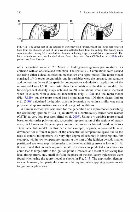
of a detonation wave at 2.5 Mach in hydrogen�oxygen�argon mixtures, its

collision with an obstacle and reflection. The spatially 2D simulations were carried

out using either a detailed reaction mechanism or a repro-model. The repro-model

consisted of 4th-order polynomials, and its variables were the pressure, temperature

and conversion factor β. In spatially homogeneous calculations, application of the

repro-model was 1,500 times faster than the simulation of the detailed model. The

time-dependent density maps obtained in 2D simulations were almost identical

when calculated with a detailed mechanism (Fig. 7.12a) and the repro-model

(Fig. 7.12b), but the repro-model-based simulation was 100 times faster. Imbert

et al. (2008) calculated the ignition times in detonation waves in a similar way using

polynomial approximations over a wide range of conditions.

A similar method was also used for the generation of a repro-model describing

the oscillatory ignition of CO–H2 mixtures in a continuously stirred tank reactor

(CSTR) at very low pressures (Brad et al. 2007). Using a 4-variable repro-model

based on 6th-order polynomials, successful representation of the regions of steady

state, cool flames and large temperature oscillations was achieved based on fits to a

14-variable full model. In this particular example, separate repro-models were

developed for different regions of the concentration/temperature space due to the

need to control fitting errors to a very high degree of accuracy in some regions. For

example, within low-temperature regions at the start of the ignition period, smaller

partitioned sets were required in order to achieve local fitting errors as low as 0.1 %.

It was found that in such regions, small differences in predicted concentrations

could lead to large shifts in the ignition point. However, as a result of achieving low

local fitting errors, only small shifts in the phase of the oscillatory trajectories were

found when using the repro-model as shown in Fig. 7.13. The application demon-

strates, however, that particular care may be required when applying repro-models

to ignition applications.

Fig. 7.12 The upper part of the detonation wave travelled further, whilst the lower part reflected

back from the obstacle. A part of the wave also reflected back from the ceiling. The density maps

were calculated using (a) a detailed mechanism including 9 species and (b) a repro-model. The

latter calculation was one hundred times faster. Reprinted from Clifford et al. (1998) with



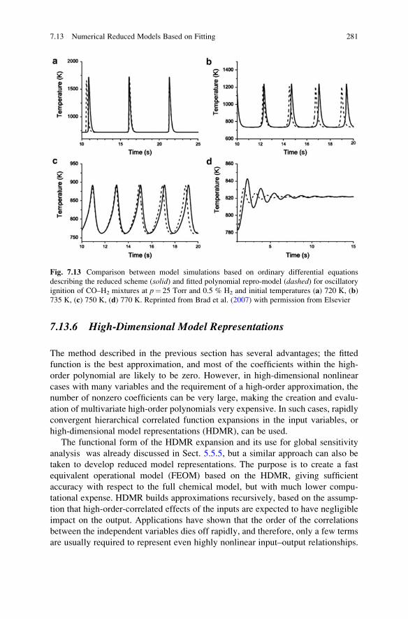
7.13.6 High-Dimensional Model Representations

The method described in the previous section has several advantages; the fitted

function is the best approximation, and most of the coefficients within the high-

order polynomial are likely to be zero. However, in high-dimensional nonlinear

cases with many variables and the requirement of a high-order approximation, the

number of nonzero coefficients can be very large, making the creation and evalu-

ation of multivariate high-order polynomials very expensive. In such cases, rapidly

convergent hierarchical correlated function expansions in the input variables, or

high-dimensional model representations (HDMR), can be used.

The functional form of the HDMR expansion and its use for global sensitivity

analysis was already discussed in Sect. 5.5.5, but a similar approach can also be

taken to develop reduced model representations. The purpose is to create a fast

equivalent operational model (FEOM) based on the HDMR, giving sufficient

accuracy with respect to the full chemical model, but with much lower compu-

tational expense. HDMR builds approximations recursively, based on the assump-

tion that high-order-correlated effects of the inputs are expected to have negligible

impact on the output. Applications have shown that the order of the correlations

between the independent variables dies off rapidly, and therefore, only a few terms

are usually required to represent even highly nonlinear input–output relationships.

Fig. 7.13 Comparison between model simulations based on ordinary differential equations

describing the reduced scheme (solid) and fitted polynomial repro-model (dashed) for oscillatoryignition of CO–H2 mixtures at p¼ 25 Torr and 0.5 % H2 and initial temperatures (a) 720 K, (b)

735 K, (c) 750 K, (d) 770 K. Reprinted from Brad et al. (2007) with permission from Elsevier



Tests on several systems including application to a stratospheric chemical model

(Shorter et al. 1999) and a tropospheric alkane oxidation model (Wang et al. 2005)

indicate that the few lowest-order terms are often sufficient to represent the model

in equivalent form to good accuracy. The approach was applied in Li et al. (2008b)

to the simulation of ignition within homogeneous H2/air mixtures over wide ranges

of temperatures and pressures (1,000< T0< 1,500 K, 0.1<P< 100 atm) and in

Gomez and Tchijov (2010) to a 3-dimensional model describing the diffusion and

advection of reactive air pollutants.

The application of HDMR tools can therefore dramatically reduce the compu-

tational effort needed to represent the input–output relationships of a physical

system. One potential advantage of such methods is that only low-order expansion

functions or coefficients must be stored, and therefore, for high-dimensional sys-

tems, storage requirements may potentially be low compared to standard tabulation

and potentially even adaptive tabulation methods. In order to reduce computational

effort, the terms in the expansion are usually represented by fitted orthogonal

polynomial functions (Li et al. 2002). The successful application of these methods

in chemically reactive atmospheric models (Wang et al. 2001) suggests their

potential for success within other applications of chemical kinetic modelling. The

methods could be coupled with ILDM-based or other methods for the selection of

key model variables in order to reduce the number of functional expansions

required (Tomlin et al. 2001). Additional information may also be obtained from

the terms in the expansion which reveal cooperations between variables and

highlight the extent of nonlinearity of the input–output relationships. As with all

operational model representations, the success of the HDMR method depends on

using a large enough region of the input variable phase space so as to be relevant in

the full model. None of these fitting methods should be expected to extrapolate well

to new conditions outside of the fitted region.

7.13.7 Artificial Neural Networks

Artificial neural networks (ANNs) are designed to attempt to recreate the way a

human brain works by constructing a network of neurons or nodes linked to each

other by a series of “synapses”. This artificial model of a brain can then be “trained”

by presenting it with examples and adjusting the effect the neurons have on each

other until the system “recognises” the examples. Through this process, ANNs have

been successfully used in image recognition and for modelling systems where

governing equations are yet to be developed or require excessive computing

power to solve. Therefore, the ANNs should be in principle capable of representing

highly nonlinear functions such as those which arise in chemical kinetic systems. A

schematic diagram of the architecture of an ANN with 2 input neurons, two hidden

layers of 6 neurons each and 3 output neurons is given in Fig. 7.14. The strengths of

connections between the different neurons are stored as weights which are deter-

mined by an appropriate learning algorithm.


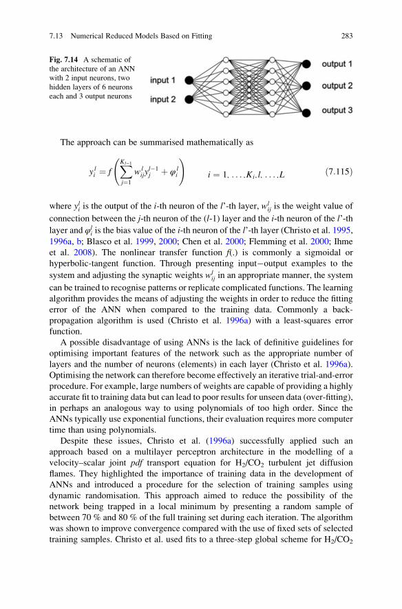
The approach can be summarised mathematically as

y li ¼ fXKl�1

j¼1

wlijy

l�1j þ φ l

i

!i ¼ 1, . . . ,Ki, l, . . . ,L ð7:115Þ

where yli is the output of the i-th neuron of the l’-th layer, wlij is the weight value of

connection between the j-th neuron of the (l-1) layer and the i-th neuron of the l’-thlayer and φl

i is the bias value of the i-th neuron of the l’-th layer (Christo et al. 1995,1996a, b; Blasco et al. 1999, 2000; Chen et al. 2000; Flemming et al. 2000; Ihme

et al. 2008). The nonlinear transfer function f(.) is commonly a sigmoidal or

hyperbolic-tangent function. Through presenting input�output examples to the

system and adjusting the synaptic weights wlij in an appropriate manner, the system

can be trained to recognise patterns or replicate complicated functions. The learning

algorithm provides the means of adjusting the weights in order to reduce the fitting

error of the ANN when compared to the training data. Commonly a back-

propagation algorithm is used (Christo et al. 1996a) with a least-squares error

function.

A possible disadvantage of using ANNs is the lack of definitive guidelines for

optimising important features of the network such as the appropriate number of

layers and the number of neurons (elements) in each layer (Christo et al. 1996a).

Optimising the network can therefore become effectively an iterative trial-and-error

procedure. For example, large numbers of weights are capable of providing a highly

accurate fit to training data but can lead to poor results for unseen data (over-fitting),

in perhaps an analogous way to using polynomials of too high order. Since the

ANNs typically use exponential functions, their evaluation requires more computer

time than using polynomials.

Despite these issues, Christo et al. (1996a) successfully applied such an

approach based on a multilayer perceptron architecture in the modelling of a

velocity–scalar joint pdf transport equation for H2/CO2 turbulent jet diffusion

flames. They highlighted the importance of training data in the development of

ANNs and introduced a procedure for the selection of training samples using

dynamic randomisation. This approach aimed to reduce the possibility of the

network being trapped in a local minimum by presenting a random sample of

between 70 % and 80 % of the full training set during each iteration. The algorithm

was shown to improve convergence compared with the use of fixed sets of selected

training samples. Christo et al. used fits to a three-step global scheme for H2/CO2

Fig. 7.14 A schematic of

the architecture of an ANN

with 2 input neurons, two

hidden layers of 6 neurons

each and 3 output neurons


combustion in their application so that detailed comparisons with the solution of the

kinetic equations and the use of look-up tables could be afforded within the

turbulent calculation. Later applications combine low-dimensional manifold theory

with fitting methods potentially giving greater accuracy for a similar number of

variables since prior assumptions have not been made in allowing reduction to a

global scheme.

Other examples of the application of ANNs include methane combustion in a

zero-dimensional calculation (Blasco et al. 1998) using a four-step global scheme,

where additional ANNs for density and temperature were included. Here a second-

order scaled-conjugate-gradient method was used instead of a back-propagation

algorithm. Again sensitivity to the training set was noted, and particular care was

taken to avoid the inclusion of data points close to steady-state regions. A compar-

ison of different ANN architectures was given in this work with either one or two

hidden layers with up to 20 neurons in each. The error of the test data set was shown

to decrease with the number of hidden neurons up to 20 in two hidden layers for

species composition, but above this the error in some cases increased. The expla-

nation given is that the ANN is more likely to get trapped in a local minimum as the

error surface becomes more complex with increasing numbers of neurons. Again

this demonstrates that care must be taken in the design of the ANN architecture. In

this particular case, tabulated chemistry was shown to give a bigger speed-up than

the ANN with regard to computational effort to solve the chemical submodel,

although at the expense of requiring substantially more memory. Both the ANN

and tabulated models provided significant speed-up compared to integration of the

full chemical rate equations. The work was further developed in Blasco et al. (1999)

where the accuracy of the ANN was improved by fitting separate networks to

subdomains of chemical composition space.

Defining optimal subdomains for which to develop the replacement models is a

key component of balancing accuracy, and storage and retrieval efficiency. In order

to address this problem, Blasco et al. attempted to develop an automatic method for

partitioning thermochemical space into optimal domains based on a self-organising

map (SOM) approach (Blasco et al. 2000). The SOM performs a mapping between

the high-dimensional thermochemical space and a two-dimensional (2D) map

whilst attempting to preserve the topology of the original space. The idea is to

ensure that points which are close to each other in the original space remain so in

the equivalent 2D space. The SOM is then used in the retrieval stage to define which

ANN to be used. Three different resolutions of subdomains with 16, 100 and

400 regions were tested, based on each mass fraction and the time step, as opposed

to just the mixture fraction tested in previous work. A multilayer perceptron

technique was then used to fit ANNs to each subdomain. The use of 100 subdomains

with 10 or 20 hidden neurons was shown to give the lowest overall error. The use of

subdomains was shown to substantially reduce the error compared to a single ANN

across for the whole thermochemical space, as well as the CPU effort required in

training the ANNs. This is analogous to the subdomain strategy used in the

orthonormal polynomial fitting in Brad et al. (2007) discussed above. The CPU


requirements of retrieval are equivalent for the two approaches suggesting that the

use of subdomains is a successful strategy.

The use of ANNs has been coupled with several other available reduction

methods. For example, in Chen et al. (2000), ANNs were used to fit the outcome

of the ISAT method, the idea being to reduce the storage requirements compared to

the usual look-up tables used in ISAT which is based on tabulated data and linear

interpolation. The use of nonlinear functions incorporated into the ANN approach

therefore facilitates single fits over a wider region than the ellipsoid of accuracy

(EOA) used in the original ISAT method. Here, the trade-off is between the fact that

the ISAT method contains exact solution values at the tabulated points with

potentially small interpolation errors where a small EOA is used, compared to

potentially larger fitting errors but much smaller tabulation requirements of ANNs.

There is also a potential overhead in selecting the optimal ANN architecture. The

CPU requirements of both methods were comparable for the partially stirred reactor

example explored in this work (Chen et al. 2000). In general, the optimal method

may well depend on the individual application and accuracy and memory

requirements.

Shenvi et al. (2004) applied neural networks based on a simple multivariate

polynomial architecture. The accuracy and efficiency of these ridge polynomial

networks were demonstrated by modelling the kinetics of H2–Br2 reaction, form-

aldehyde oxidation and H2–O2 combustion. Choi and Chen (2005) also applied

ANNs for the prediction of ignition delay times in homogeneously charged com-

pression ignition (HCCI) engine combustion for a range of fuels including propane

and iso-octane in a well-mixed reactor. Dyer and Korakianitis (2007) simulated

propane�air detonation by representing heat release and species information during

the reaction via a mapping methodology. Multilayer feedforward neural networks

were used as function approximators to reproduce the parameters extracted from

the detailed integrations and to perform the nonlinear interpolations required

between reaction points. The mapping method results were accurate to within 1–

3 % compared to the results of detailed integrations, and the computational effort

was reduced by two orders of magnitude.

Ihme et al. (2009) carried out large eddy simulations of a methane�hydrogen

flame by employing two chemistry representation methods, the conventional struc-

tured tabulation technique and ANNs. The latter was based on the optimal artificial

neural networks (OANNs) approach (Ihme et al. 2008). It was demonstrated that the

ANN accuracies were comparable with the use of structured tables. Compared to

the tabulation technique, data retrieval from the network was computationally

slightly more expensive. Zhou et al. (2013) applied ANNs for both chemical

kinetics reduction and source term evaluation in direct numerical simulation

(DNS) and large eddy simulation (LES) of reactive flows. The ANNs were trained

with 1D disturbed flames. Then, back-propagation ANNs were used for DNS and

LES modelling of H2/air and C3H8/air premixed flames with various levels of

turbulence. Mirgolbabaei and Echekki (2014) used ANN representation in conjunc-

tion with the reduction of the composition space with kernel principal component

analysis.


In Chatzopoulos and Rigopoulos (2013), the use of ANNs was combined with

the rate-controlled constrained equilibrium (RCCE) approach (see Sect. 7.10.4) in

models of two non-premixed and non-piloted CH4/H2/N2 turbulent flames. Large

computational speed-ups were reported, with reasonable agreement in the simu-

lation of major chemical species with respect to the full integration of the kinetic

scheme. Some discrepancies were observed for the minor species, but the work

indicates a potential of RCCE–ANN tabulation methodologies for future turbulent

combustion computations.

7.13.8 Piecewise Reusable Maps (PRISM)

The functional mappings used to represent the solution of the chemical kinetic

differential equations (i.e. the surrogate or repro-model) are usually prepared and

fitted prior to the final intended simulations within, for example, complex

multidimensional reactive flow codes. Using the ISAT approach described in

Sect. 7.12.2, the tabulation is achieved during the simulation, with the advantage

that only accessed regions of composition space have to be tabulated. A similar

method, but using polynomial fits, is the PRISM (piecewise reusable imple-

mentation of solution mapping) approach (Tonse et al. 1999) whereby the fitted

polynomial functions are developed during the calculation and then reused when

the region of composition space is revisited in subsequent time steps or different

spatial regions. PRISM uses second-order polynomials so that in order to cover the

realisable region, multiple expressions are used, each valid over a different portion

of composition space. This is achieved by partitioning the chemical composition

space into predetermined non-overlapping adjacent hypercubes, with edges and

corners permitted at regular intervals along the axes allowing for the simple

indexing required for efficient searching during reuse. Integration of the full kinetic

equations then provides the solution at selected points throughout a hypercube, in

order to determine the polynomial coefficients. Factorial design methods are used to

reduce the required number of computed points. Not surprisingly Tonse et al. report

an increase in accuracy with reduced hypercube size. In common with other

methods, however, there is a trade-off between accuracy and the efficiency of

polynomial generation as well as storage and retrieval. The largest hypercubes

achievable should be used to minimise the computational effort required. Improve-

ments to efficiency were suggested in Tonse et al. (2003)and Brown and Tonse

(2004) based on two alternative methods for the a priori identification of hyper-

cubes that will have a high level of reuse. This allows for polynomial construction

only for those hypercubes that are revisited enough times to make the construction

worthwhile. The PRISM method has demonstrated successful application to hydro-

gen ignition, a 1D laminar hydrogen flame, a 2D axisymmetric turbulent jet (Tonse

et al. 1999, 2003) and a turbulent premixed hydrogen flame (Bell et al. 2000). In a

similar way to the other repro-modelling methods, the constructed polynomials

could potentially be stored for other calculations as long as the fitted regions of


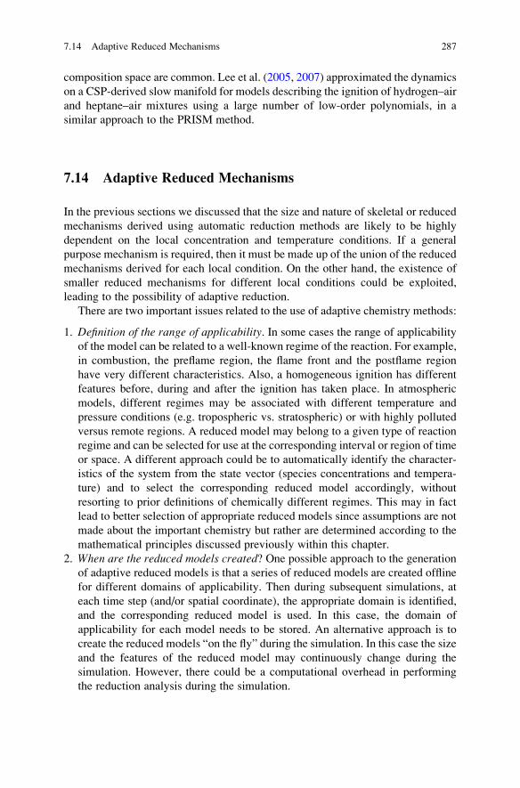
composition space are common. Lee et al. (2005, 2007) approximated the dynamics

on a CSP-derived slow manifold for models describing the ignition of hydrogen–air

and heptane–air mixtures using a large number of low-order polynomials, in a

similar approach to the PRISM method.

7.14 Adaptive Reduced Mechanisms

In the previous sections we discussed that the size and nature of skeletal or reduced

mechanisms derived using automatic reduction methods are likely to be highly

dependent on the local concentration and temperature conditions. If a general

purpose mechanism is required, then it must be made up of the union of the reduced

mechanisms derived for each local condition. On the other hand, the existence of

smaller reduced mechanisms for different local conditions could be exploited,

leading to the possibility of adaptive reduction.

There are two important issues related to the use of adaptive chemistry methods:

1. Definition of the range of applicability. In some cases the range of applicability

of the model can be related to a well-known regime of the reaction. For example,

in combustion, the preflame region, the flame front and the postflame region

have very different characteristics. Also, a homogeneous ignition has different

features before, during and after the ignition has taken place. In atmospheric

models, different regimes may be associated with different temperature and

pressure conditions (e.g. tropospheric vs. stratospheric) or with highly polluted

versus remote regions. A reduced model may belong to a given type of reaction

regime and can be selected for use at the corresponding interval or region of time

or space. A different approach could be to automatically identify the character-

istics of the system from the state vector (species concentrations and tempera-

ture) and to select the corresponding reduced model accordingly, without

resorting to prior definitions of chemically different regimes. This may in fact

lead to better selection of appropriate reduced models since assumptions are not

made about the important chemistry but rather are determined according to the

mathematical principles discussed previously within this chapter.

2. When are the reduced models created? One possible approach to the generation

of adaptive reduced models is that a series of reduced models are created offline

for different domains of applicability. Then during subsequent simulations, at

each time step (and/or spatial coordinate), the appropriate domain is identified,

and the corresponding reduced model is used. In this case, the domain of

applicability for each model needs to be stored. An alternative approach is to

create the reduced models “on the fly” during the simulation. In this case the size

and the features of the reduced model may continuously change during the

simulation. However, there could be a computational overhead in performing

the reduction analysis during the simulation.

7.14 Adaptive Reduced Mechanisms 287

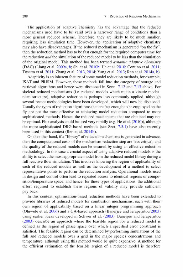
The application of adaptive chemistry has the advantage that the reduced

mechanisms used have to be valid over a narrower range of conditions than a

more general reduced scheme. Therefore, they are likely to be much smaller,

requiring less simulation time. However, the application of adaptive chemistry

may also have disadvantages. If the reduced mechanism is generated “on the fly”,

then the reduction method has to be fast enough for the required computer time for

the reduction and the simulation of the reduced model to be less than the simulation

of the original model. This method has been termed dynamic adaptive chemistry(DAC) (Liang et al. 2009a, b; Shi et al. 2010b; He et al. 2010; Contino et al. 2011;

Tosatto et al. 2011; Zhang et al. 2013, 2014; Yang et al. 2013; Ren et al. 2014a, b).

Adaptivity is an inherent feature of some model reduction methods, for example,

ISAT and PRISM. However, these methods fall into the category of storage and

retrieval algorithms and hence were discussed in Sects. 7.12 and 7.13 above. For

skeletal reduced mechanisms (i.e. reduced models which retain a kinetic mecha-

nism structure), adaptive reduction is perhaps less commonly applied, although

several recent methodologies have been developed, which will now be discussed.

Usually the types of reduction algorithms that are fast enough to be employed on the

fly are not the most effective at achieving model reduction compared to more

sophisticated methods. Hence, the reduced mechanisms that are obtained may not

be optimal. Flux analysis could be used very rapidly (e.g. He et al. (2010)), although

the more sophisticated DRG-based methods (see Sect. 7.5.1) have also recently

been used in this context (Ren et al. 2014b).

On the other hand, if a “library” of reduced mechanisms is generated in advance,

then the computational costs of the mechanism reduction step are less critical, and

the quality of the reduced models can be ensured by using an effective reduction

methodology. In this case a crucial aspect of using adaptive reduced models is the

ability to select the most appropriate model from the reduced model library during a

full reactive flow simulation. This involves knowing the region of applicability of

each of the reduced models as well as the development of a method to select

representative points to perform the reduction analysis. Operational models used

in design and control often lead to repeated access to identical regions of compo-

sition/temperature space, and hence, for these types of applications, the additional

effort required to establish these regions of validity may provide sufficient

pay back.

In this context, optimisation-based reduction methods have been extended to

provide libraries of reduced models for combustion mechanisms, each with their

own region of applicability based on a linear integer programming approach

(Oluwole et al. 2006) and a GA-based approach (Banerjee and Ierapetritou 2003)

using earlier ideas developed in Schwer et al. (2003). Banerjee and Ierapetritou

(2003) describe an approach where the feasible region for a reduced model is

defined as the region of phase space over which a specified error constraint is

satisfied. The feasible region can be determined by performing simulations of the

full and reduced models over a grid in the major species concentrations and

temperature, although using this method would be quite expensive. A method for

the efficient estimation of the feasible region of a reduced model is therefore


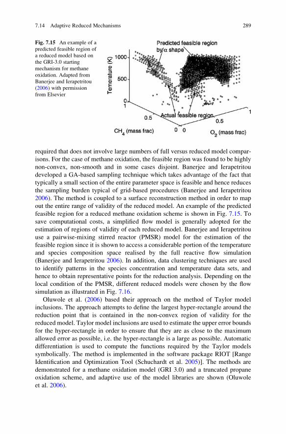
required that does not involve large numbers of full versus reduced model compar-

isons. For the case of methane oxidation, the feasible region was found to be highly

non-convex, non-smooth and in some cases disjoint. Banerjee and Ierapetritou

developed a GA-based sampling technique which takes advantage of the fact that

typically a small section of the entire parameter space is feasible and hence reduces

the sampling burden typical of grid-based procedures (Banerjee and Ierapetritou

2006). The method is coupled to a surface reconstruction method in order to map

out the entire range of validity of the reduced model. An example of the predicted

feasible region for a reduced methane oxidation scheme is shown in Fig. 7.15. To

save computational costs, a simplified flow model is generally adopted for the

estimation of regions of validity of each reduced model. Banerjee and Ierapetritou

use a pairwise-mixing stirred reactor (PMSR) model for the estimation of the

feasible region since it is shown to access a considerable portion of the temperature

and species composition space realised by the full reactive flow simulation

(Banerjee and Ierapetritou 2006). In addition, data clustering techniques are used

to identify patterns in the species concentration and temperature data sets, and

hence to obtain representative points for the reduction analysis. Depending on the

local condition of the PMSR, different reduced models were chosen by the flow

simulation as illustrated in Fig. 7.16.

Oluwole et al. (2006) based their approach on the method of Taylor model

inclusions. The approach attempts to define the largest hyper-rectangle around the

reduction point that is contained in the non-convex region of validity for the

reduced model. Taylor model inclusions are used to estimate the upper error bounds

for the hyper-rectangle in order to ensure that they are as close to the maximum

allowed error as possible, i.e. the hyper-rectangle is a large as possible. Automatic

differentiation is used to compute the functions required by the Taylor models

symbolically. The method is implemented in the software package RIOT [Range

Identification and Optimization Tool (Schuchardt et al. 2005)]. The methods are

demonstrated for a methane oxidation model (GRI 3.0) and a truncated propane

oxidation scheme, and adaptive use of the model libraries are shown (Oluwole

et al. 2006).

Fig. 7.15 An example of a

predicted feasible region of

a reduced model based on

the GRI-3.0 starting

mechanism for methane

oxidation. Adapted from

Banerjee and Ierapetritou

(2006) with permission

from Elsevier

7.14 Adaptive Reduced Mechanisms 289

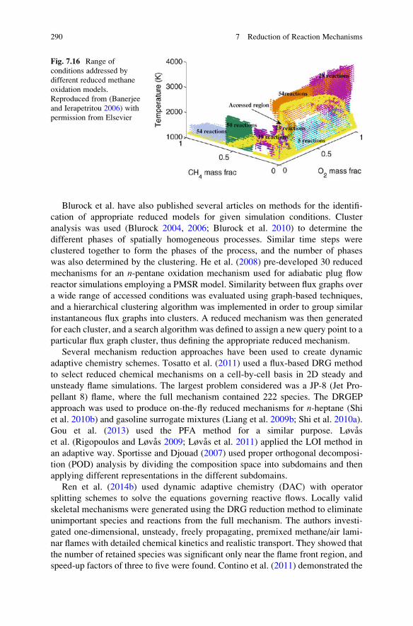
Blurock et al. have also published several articles on methods for the identifi-

cation of appropriate reduced models for given simulation conditions. Cluster

analysis was used (Blurock 2004, 2006; Blurock et al. 2010) to determine the

different phases of spatially homogeneous processes. Similar time steps were

clustered together to form the phases of the process, and the number of phases

was also determined by the clustering. He et al. (2008) pre-developed 30 reduced

mechanisms for an n-pentane oxidation mechanism used for adiabatic plug flow

reactor simulations employing a PMSR model. Similarity between flux graphs over

a wide range of accessed conditions was evaluated using graph-based techniques,

and a hierarchical clustering algorithm was implemented in order to group similar

instantaneous flux graphs into clusters. A reduced mechanism was then generated

for each cluster, and a search algorithm was defined to assign a new query point to a

particular flux graph cluster, thus defining the appropriate reduced mechanism.

Several mechanism reduction approaches have been used to create dynamic

adaptive chemistry schemes. Tosatto et al. (2011) used a flux-based DRG method

to select reduced chemical mechanisms on a cell-by-cell basis in 2D steady and

unsteady flame simulations. The largest problem considered was a JP-8 (Jet Pro-

pellant 8) flame, where the full mechanism contained 222 species. The DRGEP

approach was used to produce on-the-fly reduced mechanisms for n-heptane (Shi

et al. 2010b) and gasoline surrogate mixtures (Liang et al. 2009b; Shi et al. 2010a).

Gou et al. (2013) used the PFA method for a similar purpose. Løvas

et al. (Rigopoulos and Løvas 2009; Løvas et al. 2011) applied the LOI method in

an adaptive way. Sportisse and Djouad (2007) used proper orthogonal decomposi-

tion (POD) analysis by dividing the composition space into subdomains and then

applying different representations in the different subdomains.

Ren et al. (2014b) used dynamic adaptive chemistry (DAC) with operator

splitting schemes to solve the equations governing reactive flows. Locally valid

skeletal mechanisms were generated using the DRG reduction method to eliminate

unimportant species and reactions from the full mechanism. The authors investi-

gated one-dimensional, unsteady, freely propagating, premixed methane/air lami-

nar flames with detailed chemical kinetics and realistic transport. They showed that

the number of retained species was significant only near the flame front region, and

speed-up factors of three to five were found. Contino et al. (2011) demonstrated the

Fig. 7.16 Range of

conditions addressed by

different reduced methane

oxidation models.

Reproduced from (Banerjee

and Ierapetritou 2006) with



coupling of in situ adaptive tabulation and dynamic adaptive chemistry for engine

simulations. Dynamic adaptive chemistry-based models were successfully used in

general turbulent reactive flow simulations (Yang et al. 2013; Ren et al. 2014a).

Lu et al. (2009) identified QSS-species and pre-equilibrium reactions on the fly,

based on the investigation of system timescales. This information was used to

convert the original system of differential equations to a less stiff system of

differential algebraic equations. This dynamic stiffness removal method for accel-

erating simulations was successfully applied for predictions using an n-heptaneoxidation mechanism in 1D and 2D turbulent direct numerical simulations.

Oluwole et al. (2012) developed a new variant of adaptive chemistry called

exact-steady-state adaptive chemistry (ESAC). This method is applicable for fast

reduced model simulations of steady-state problems. Smaller (less accurate, but

faster) reduced models are used when the simulation is far from the steady state,

whilst more accurate (larger and slower) models are used as the simulation

approaches the final steady-state solution. The simulation is completed by applying

the full kinetic model for the calculation of the steady-state solution. ESAC

simulations were found to be a factor of 3–4 times faster than the equivalent full-

model-everywhere simulations. Such techniques could be valuable, for example, in

obtaining solutions for 2D or 3D computational fluid dynamics simulations of

steady problems which are often slow to converge when using highly detailed

chemistry. Oluwole et al. (2012) demonstrated application of the method for 2D

steady methane and ethylene flames.

So far, the use of adaptive reduced models has mainly focused on reaction

removal leading to, at best, linear reductions in computational time (Harris

et al. 2000). In this case the same set of ODEs are solved at each time step, and

the computational savings are made due to the lower number of operations neces-

sary to perform Jacobian evaluations when a large number of the reaction terms

have been removed. Further challenges are presented for species removal since the

number of species may change in each reduced model region. In an operator

splitting environment (see Sect. 6.8), where the flow and chemistry steps are solved

separately, a simple solution is to consider all the species of the detailed mechanism

in the flow step and only those species present in the selected reduced model in the

chemistry step, with the concentration of all the other species unaltered. Banerjee

and Ierapetritou (2003) successfully used this approach for a methane oxidation

mechanism where up to 12 reduced models are accessed during the model simula-

tions with the number of chemically active species varying between 6 and 29.

References

Ahmed, S.S., Mauß, F., Moreacz, G., Zeuch, T.: A comprehensive and compact n-heptane

oxidation model derived using chemical lumping. PCCP 9, 1107–1126 (2007)

Al-Khateeb, A.N., Powers, J.M., Paolucci, S., Sommese, A.J., Diller, J.A., Hauenstein, J.D.,

Mengers, J.D.: One-dimensional slow invariant manifolds for spatially homogenous reactive

systems. J. Chem. Phys. 131, 024118 (2009)

References 291


An, J., Jiang, Y.: Differences between direct relation graph and error-propagation-based reduction

methods for large hydrocarbons. Procedia Eng. 62, 342–349 (2013)

Anderson, J., Chang, Y.-C., Papachristodoulou, A.: Model decomposition and reduction tools for

large-scale networks in systems biology. Automatica 47, 1165–1174 (2011)

Androulakis, I.P.: Kinetic mechanism reduction based on an integer programming approach.

AIChE J. 46, 361–371 (2000)

Androulakis, I.P.: “Store and retrieve” representations of dynamic systems motivated by studies in

gas phase chemical kinetics. Comput. Chem. Eng. 28, 2141–2155 (2004)

Androulakis, I.P., Grenda, J.M., Bozzelli, J.W.: Time-integrated pointers for enabling the analysis

of detailed reaction mechanisms. AIChE J. 50, 2956–2970 (2004)

Apri, M., de Gee, M., Molenaar, J.: Complexity reduction preserving dynamical behavior of

biochemical networks. J. Theor. Biol. 304, 16–26 (2012)

Apri, M., de Gee, M., van Mourik, S., Molenaar, J.: Identifying optimal models to represent

biochemical systems. PLoS One 9, e83664 (2014)

Aris, R.: Reactions in continous mixtures. AIChE J. 35, 539–548 (1989)

Aris, R., Gavalas, G.R.: On the theory of reactions in continuous mixtures. Philos. Trans. R. Soc.

A260, 351–393 (1966)

Astarita, G.: Lumping nonlinear kinetics: apparent overall order of reaction. AIChE J. 35, 529–532

(1989)

Astarita, G., Nigam, A.: Lumping nonlinear kinetics in a CSTR. AIChE J. 35, 1927–1932 (1989)

Astarita, G., Ocone, R.: Lumping nonlinear kinetics. AIChE J. 34, 1299–1309 (1986)

Astarita, G., Ocone, R.: Chemical reaction engineering of complex mixtures. Chem. Eng. Sci. 47,

2135–2147 (1992)

Astarita, G., Sandler, S.I. (eds.): Kinetic and Thermodynamic Lumping of Multicomponent

Mixtures. Elsevier, Amsterdam (1991)

Atanga, G.F.: Direct numerical simulation of turbulent flames on parallel computers. Ph.D. thesis,

Otto-von-Guericke-Universitat (2012)

Austin, J.: On the explicit versus family solution of the fully diurnal photochemical equations of

the stratosphere. J. Geophys. Res. Atmos. 96(D7), 12941–12974 (1991)

Bahlouli, K., Atikol, U., Saray, R.K., Mohammadi, V.: A reduced mechanism for predicting the

ignition timing of a fuel blend of natural-gas and n-heptane in HCCI engine. Energy Convers.

Manage. 79, 85–96 (2014)

Bailey, J.E.: Lumping analysis of reactions in continuous mixtures. Chem. Eng. J. 3, 52–71 (1972)

Banerjee, I., Ierapetritou, M.G.: Development of an adaptive chemistry model considering

micromixing effects. Chem. Eng. Sci. 58, 4537–4555 (2003)

Banerjee, I., Ierapetritou, M.G.: An adaptive reduction scheme to model reactive flow. Combust.

Flame 144, 619–633 (2006)

Battin-Leclerc, F., Glaude, P.A., Warth, V., Fournet, R., Scacchi, G., Come, G.M.: Computer tools

for modelling the chemical phenomena related to combustion. Chem. Eng. Sci. 55, 2883–2893

(2000)

Becker, T., Weispfenning, V.: Grobner Bases (A Computational Approach to Communicative

Algebra). Springer, New York (1993)

Bekdemir, C., Somers, L.M.T., de Goey, L.P.H.: Modeling diesel engine combustion using

pressure dependent Flamelet generated manifolds. Proc. Combust. Inst. 33, 2887–2894 (2011)

Bell, J.B., Brown, N.J., Day, M.S., Frenklach, M., Grcar, J.F., Propp, R.M., Tonse, S.R., Wagner,

A.: Scaling and efficiency of PRISM in adaptive simulations of turbulent premixed flames.


Benson, S.W.: The induction period in chain reactions. J. Chem. Phys. 20, 1605–1612 (1952)

Beretta, G.P., Keck, J.C., Janbozorgi, M., Metghalchi, H.: The rate-controlled constrained-equi-

librium approach to far-from-local-equilibrium thermodynamics. Entropy 14, 92–130 (2012)

Bhattacharjee, B., Schwer, D.A., Barton, P.I., Green, W.H.: Optimally-reduced kinetic models:

reaction elimination in large-scale kinetic mechanisms. Combust. Flame 135, 191–208 (2003)


Bilgari, A., Sutherland, J.C.: A filter-independent model identification technique for turbulent

combustion modeling. Combust. Flame 159, 1960–1970 (2012)

Bilger, R.W.: On reduced mechanisms for methane-air combustion in non-premixed flames.

Combust. Flame 80, 135–149 (1990)

Blasco, J.A., Fueyo, N., Dopazo, C., Ballester, J.: Modelling the temporal evolution of a reduced

combustion chemical system with an artificial neural network. Combust. Flame 113, 38–52

(1998)

Blasco, J.A., Fueyo, N., Larroya, J.C., Dopazo, C., Chen, Y.J.: A single-step time-integrator of a

methane–air chemical system using artificial neural networks. Comput. Chem. Eng. 23, 1127–

1133 (1999)

Blasco, J.A., Fueyo, N., Dopazo, C., Chen, J.-Y.: A self-organizing-map approach to chemistry

representation in combustion applications. Combust. Theory Model. 4, 61–76 (2000)

Blasenbrey, T., Maas, U.: ILDMs of higher hydrocarbons and the hierarchy of chemical kinetics.


Blasenbrey, T.: Entwicklung und Implementierung automatisch reduzierter Reaktionsme-

chanismen fur die Verbrennung von Kohlenwasserstoffen. Ph.D. thesis, Stuttgart University

(2000)

Blouza, A., Coquel, F., Hamel, F.: Reduction of linear kinetic systems with multiple scales.


Blurock, E.S.: Characterizing complex reaction mechanisms using machine learning clustering

techniques. Int. J. Chem. Kinet. 36, 107–118 (2004)

Blurock, E.S.: Automatic characterization of ignition processes with machine learning clustering

techniques. Int. J. Chem. Kinet. 38, 621–633 (2006)

Blurock, E.S., Tuner, M., Mauss, F.: Phase optimized skeletal mechanisms for engine simulations.


Bodenstein, M.: Eine Theorie der photochemischen Reaktionsgeschwindigkeiten. Z. Phys. Chem.

85, 329–397 (1913)

Bodenstein, M., Lutkemeyer, H.: Die photochemische Bildung von Bromwasserstoff und die

Bildungsgeschwindigkeit der Brommolekel—aus den Atomen. Z. Phys. Chem. 114, 208–236

(1924)

Bogaevski, V.N., Povzner, A.: Algebraic Method in Nonlinear Perturbation Theory. Springer,

New York (1991)

Bongers, H., Van Oijen, J.A., De Goey, L.P.H.: Intrinsic low-dimensional manifold method

extended with diffusion. Proc. Combust. Inst. 29, 1371–1378 (2002)

Bongers, H., van Oijen, J.A., de Goey, L.P.H.: The Flamelet generated manifold method applied to

steady planar partially premixed counterflow flames. Combust. Sci. Technol. 177, 2373–2393

(2005)

Borger, I., Merkel, A., Lachmann, J., Spangenberg, H.-J., Turanyi, T.: An extended kinetic model

and its reduction by sensitivity analysis for the methanol/oxygen gas-phase thermolysis. Acta

Chim. Hung. 129, 855–864 (1992)

Borghans, J.A.M., De Boer, R.J., Segel, L.A.: Extending the quasi-steady state approximation by

changing variables. Bull. Math. Biol. 58, 43–63 (1996)

Boulier, F., Lefranc, M., Lemaire, F., Morant, P.-E.: Model reduction of chemical reaction systems

using elimination. Math. Comput. Sci. 5, 289 (2011)

Bounaceur, R., Warth, V., Glaude, P.A., Battin-Leclerc, F., Scacchi, G., Come, G.M., Faravelli, T.,

Ranzi, E.: Chemical lumping of mechanisms generated by computer—Application to the

modeling of normal-butane oxidation. J. Chim. Phys. Phys. Chim. Biol. 93, 1472–1491 (1996)

Box, G.E.P., Hunter, W.G., Hunter, J.S.: Statistics for Experiments. An Introduction to Design,

Data Analysis, and Model Building. Wiley, New York (1978)

Brad, R.B., Tomlin, A.S., Fairweather, M., Griffiths, J.F.: The application of chemical reduction

methods to a combustion system exhibiting complex dynamics. Proc. Combust. Inst. 31, 455–

463 (2007)

Briggs, G.E., Haldane, J.B.S.: A note on the kinetics of enzyme action. Biochem. J. 19, 339–339

(1925)

References 293

Brochot, C., Toth, J., Bois, F.Y.: Lumping in pharmacokinetics. J. Pharmacokinet. Pharmacodyn.

32, 719–736 (2005)

Brown, N.J., Tonse, S.R.: PRISM Piecewise reusable implementation of solution mapping to

improve computational economy. Abstr. Pap. Am. Chem. Soc. 228, U308–U308 (2004)

Buki, A., Perger, T., Turanyi, T., Maas, U.: Repro-modelling based generation of intrinsic

low-dimensional manifolds. J. Math. Chem. 31, 345–362 (2002)

Bykov, V., Gol’dshtein, V.: Fast and slow invariant manifolds in chemical kinetics. Comput.

Math. Appl. 65, 1502–1515 (2013)

Bykov, V., Maas, U.: The extension of the ILDM concept to reaction-diffusion manifolds.

Combust. Theory Model. 11, 839–862 (2007a)

Bykov, V., Maas, U.: Extension of the ILDM method to the domain of slow chemistry. Proc.

Combust. Inst. 31, 465–472 (2007b)

Bykov, V., Maas, U.: Investigation of the hierarchical structure of kinetic models in ignition

problems. Z. Phys. Chem. 223, 461–479 (2009a)

Bykov, V., Maas, U.: Problem adapted reduced models based on reaction-diffusion manifolds

(REDIMs). Proc. Combust. Inst. 32, 561–568 (2009b)

Bykov, V., Goldfarb, I., Gol’dshtein, V., Sazhin, S., Sazhina, E.: System decomposition technique

for spray modelling in CFD codes. Comput. Fluids 36, 601–610 (2007)

Bykov, V., Griffiths, J.F., Piazzesi, R., Sazhin, S.S., Sazhina, E.M.: The application of the global

quasi-linearisation technique to the analysis of the cyclohexane/air mixture autoignition. Appl.

Math. Comput. 219, 7338–7347 (2013)

Cannon, S.M., Brewster, B.S., Smoot, L.D.: PDF modeling of lean premixed combustion using in

situ tabulated chemistry. Combust. Flame 119, 233–252 (1999)

Carslaw, N., Jacobs, P.J., Pilling, M.J.: Modeling OH, HO2, and RO2 radicals in the marine

boundary layer 2. Mechanism reduction and uncertainty analysis. J. Geophys. Res. D 104,

30257–30273 (1999)

Chapman, D.L., Underhill, L.K.: The interaction of chlorine and hydrogen. The influence of mass.

J. Chem. Soc. Trans. 103, 496–508 (1913)

Chatzopoulos, A.K., Rigopoulos, S.: A chemistry tabulation approach via rate-controlled

constrained equilibrium (RCCE) and artificial neural networks (ANNs), with application to

turbulent non-premixed CH4/H2/N2 flames. Proc. Combust. Inst. 34, 1465–1473 (2013)

Chen, J.Y.: A general procedure for constructing reduced reaction-mechanisms with given inde-

pendent relations. Combust. Sci. Technol. 57, 89–94 (1988)

Chen, J.Y.: Analysis of in situ adaptive tabulation performance for combustion chemistry and

improvement with a modified search algorithm. Combust. Sci. Technol. 176, 1153–1169

(2004)

Chen, J.Y., Tham, Y.F.: Speedy solution of quasi-steady-state species by combination of fixed-

point iteration and matrix inversion. Combust. Flame 153, 634–646 (2008)

Chen, J.Y., Chang, W.C., Koszykowski, M.: Numerical simulation and scaling of NOx emissions

from turbulent hydrogen jet flames with various amounts of helium dilution. Combust. Sci.

Technol. 111, 505–529 (1995)

Chen, J.Y., Blasco, J.A., Fueyo, N., Dopazo, C.: An economical strategy for storage of chemical

kinetics: fitting in situ adaptive tabulation with artificial neural networks. Proc. Combust. Inst.

28, 115–121 (2000)

Chiavazzo, E., Gorban, A.N., Karlin, I.V.: Comparison of invariant manifolds for model reduction

in chemical kinetics. Commun. Comput. Phys. 2, 964–992 (2007)

Chiavazzo, E., Karlin, I.V., Frouzakis, C.E., Boulouchos, K.: Method of invariant grid for model

reduction of hydrogen combustion. Proc. Combust. Inst. 32, 519–526 (2009)

Choi, Y., Chen, J.Y.: Fast prediction of start-of-cornbustion in HCCI with combined artificial

neural networks and ignition delay model. Proc. Combust. Inst. 30, 2711–2718 (2005)

Chou, M.Y., Ho, T.C.: Continuum theory for lumping nonlinear reactions. AIChE J. 34, 1519–

1527 (1988)


Christo, F.C., Masri, A.R., Nebot, E.M., Turanyi, T.: Utilising artificial neural network and repro-

modelling in turbulent combustion. Proc. IEEE Int. Conf. Neural Netw. 1, 911–916 (1995)

Christo, F.C., Masri, A.R., Nebot, E.M.: Artificial neural network implementation of chemistry

with pdf Simulation of H2/CO2 flames. Combust. Flame 106, 406–427 (1996a)

Christo, F.C., Masri, A.R., Nebot, E.M., Pope, S.B.: An integrated PDF/neural network approach

for simulating turbulent reacting systems. Proc. Combust. Inst. 26, 43–48 (1996b)

Chu, Y., Serpas, M., Hahn, J.: State-preserving nonlinear model reduction procedure. Chem. Eng.

Sci. 66, 3907–3913 (2011)

Cicarelli, P., Astarita, G., Gallifuoco, A.: Continuous kinetic lumping of catalytic cracking

processes. AIChE J. 38, 1038–1044 (1992)

Ciliberto, A., Capuani, F., Tyson, J.J.: Modeling networks of coupled enzymatic reactions using

the total quasi-steady state approximation. PLoS Comput. Biol. 3, e45 (2007)

Clifford, L.J., Milne, A.M., Turanyi, T., Boulton, D.: An induction parameter model for shock-

induced hydrogen combustion simulations. Combust. Flame 113, 106–118 (1998)

Colin, O., Pires da Cruz, A., Jay, S.: Detailed chemistry-based auto-ignition model including low

temperature phenomena applied to 3-D engine calculations. Proc. Combust. Inst. 30, 2649–

2656 (2005)

Contino, F., Jeanmart, H., Lucchini, T., D’Errico, G.: Coupling of in situ adaptive tabulation and

dynamic adaptive chemistry: an effective method for solving combustion in engine simula-

tions. Proc. Combust. Inst. 33, 3057–3064 (2011)

Coussement, A., Gicquel, O., Parente, A.: Kernel density weighted principal component analysis

of combustion processes. Combust. Flame 159, 2844–2855 (2012)

Coussement, A., Gicquel, O., Parente, A.: MG-local-PCA method for reduced order combustion

modeling. Proc. Combust. Inst. 34, 1117–1123 (2013)

Crutzen, P.J.: Ozone production rates in an oxygen–hydrogen–nitrogen oxide atmosphere.

J. Geophys. Res. 76, 7311–7327 (1971)

Cunha Jr., A., da Silva, L.F.F.: Assessment of a transient homogeneous reactor through in situ

adaptive tabulation. J Braz. Soc. Mech. Sci. Eng. 36, 377–391 (2014)

Danby, S.J., Echekki, T.: Proper orthogonal decomposition analysis of autoignition simulation

data of nonhomogeneous hydrogen-air mixtures. Combust. Flame 144, 126–138 (2006)

Dano, S., Madsen, M.F., Schmidt, H., Cedersund, G.: Reduction of a biochemical model with

preservation of its basic dynamic properties. FEBS J. 273, 4862–4877 (2006)

Davis, M.J., Skodje, R.T.: Geometric investigation of low-dimensional manifolds in systems

approaching equilibrium. J. Chem. Phys. 111, 859–874 (1999)

Davis, M.J., Tomlin, A.S.: Spatial dynamics of steady flames 1. Phase space structure and the

dynamics of individual trajectories. J. Phys. Chem. A 112, 7768–7783 (2008a)

Davis, M.J., Tomlin, A.S.: Spatial dynamics of steady flames 2. Low-dimensional manifolds and

the role of transport processes. J. Phys. Chem. A 112, 7784–7805 (2008b)

Davis, S.G., Mhadeshwar, A.B., Vlachos, D.G., Wang, H.: A new approach to response surface

development for detailed gas-phase and surface reaction kinetic model optimization. Int.

J. Chem. Kinet. 36, 94–106 (2004)

de Goey, L.P.H., van Oijen, J.A., Bongers, H., Groot, G.R.A.: New flamelet based reduction

methods: the bridge between chemical reduction techniques and flamelet methods. In: Pro-

ceedings of ECM (2003)

Djouad, R., Sportisse, B.: Partitioning techniques for reduction in chemical kinetics. APLA: an

Automatic Partitioning and Lumping Algorithm. Appl. Numeric. Math. 43, 383–398 (2002)

Djouad, R., Sportisse, B., Audiffren, N.: Reduction of multiphase atmospheric chemistry. J. Atm.

Chem. 46, 131–157 (2003)

Dokoumetzidis, A., Aarons, L.: A method for robust model order reduction in pharmacokinetics.

J. Pharmacokinet. Pharmacodyn. 36, 613–628 (2009a)

Dokoumetzidis, A., Aarons, L.: Proper lumping in systems biology models. IET Syst. Biol. 3, 40–

51 (2009b)

References 295

Douglass, A.R., Kawa, S.R.: Contrast between 1992 and 1997 high-latitude spring halogen

occultation experiment observations of lower stratospheric HCl. J. Geophys. Res. Atmos.

104(D15), 18739–18754 (1999)

Dunker, A.M.: The reduction and parameterization of chemical mechanisms for inclusion in

atmospheric reaction-transport models. Atmos. Environ. 20, 479–486 (1986)

Dyer, R.S., Korakianitis, T.: Pre-integrated response map for inviscid propane-air detonation.


Edelson, D.: On the solution of differential equations arising in chemical kinetics. J. Comput.

Phys. 11, 455–457 (1973)

Edwards, K., Edgar, T.F., Manousiouthakis, V.I.: Kinetic model reduction using genetic algo-

rithms. Comput. Chem. Eng. 22, 239–246 (1998)

Edwards, K., Edgar, T.F., Manousiouthakis, V.I.: Reaction mechanism simplification using

mixed-integer nonlinear programming. Comput. Chem. Eng. 24, 67–79 (2000)

Eggels, R.L.G.M., de Goey, L.P.H.: Mathematically reduced reaction mechanisms applied to

adiabatic flat hydrogen/air flames. Combust. Flame 100, 559–570 (1995)

Elliott, S., Turco, R.P., Jacobson, M.Z.: Tests on combined projection forward differencing

integration for stiff photochemical family systems at long-time step. Comput. Chem. 17, 91–

102 (1993)

Elliott, S., Shen, M., Kao, C.Y.J., Turco, R.P., Jacobson, M.Z.: A streamlined family photochem-

istry module reproduces major nonlinearities in the global tropospheric ozone system. Comput.

Chem. 20, 235–259 (1996)

Elliott, L., Ingham, D.B., Kyne, A.G., Mera, N.S., Pourkashanian, M., Wilson, C.W.: Genetic

algorithms for optimisation of chemical kinetics reaction mechanisms. Prog. Energy Combust.

Sci. 30, 297–328 (2004)

Elliott, L., Ingham, D.B., Kyne, A.G., Mera, N.S., Pourkashanian, M., Wilson, C.W.: Reaction

mechanism reduction and optimization using genetic algorithms. Ind. Eng. Chem. Res. 44,

658–667 (2005)

Elliott, L., Ingham, D.B., Kyne, A.G., Merab, N.S., Pourkashanian, M., Whittaker, S.: Reaction

mechanism reduction and optimisation for modelling aviation fuel oxidation using standard

and hybrid genetic algorithms. Comput. Chem. Eng. 30, 889–900 (2006)

Enjalbert, N., Domingo, P., Vervisch, L.: Mixing time-history effects in large Eddy simulation of

non-premixed turbulent flames: flow-controlled chemistry tabulation. Combust. Flame 159,

336–352 (2012)

Farkas, G.: Kinetic lumping schemes. Chem. Eng. Sci. 54, 3909–3915 (1999)

Farrow, L.A., Edelson, D.: Steady-state approximation—Fact or fiction? Int. J. Chem. Kinet. 6,

787–800 (1974)

Feeley, R., Seiler, P., Packard, A., Frenklach, M.: Consistency of a reaction dataset. J. Phys. Chem.

A 108, 9573–9583 (2004)



Fiorina, B., Gicquel, O., Vervisch, L., Carpentier, S., Darabiha, N.: Approximating the chemical

structure of partially premixed and diffusion counterflow flames using FPI flamelet tabulation.

Combust. Flame 140, 147–160 (2005)

Fischer, M., Riedel, U.: Combustion chemistry and parameter estimation. In: Bock, H.G., Carraro,

T., Jager, W., Korkel, S., Rannacher, R., Schloder, J.P. (eds.) Model Based Parameter Estima-

tion. Theory and Applications, vol. 4, pp. 207–226. Springer, Berlin (2013)

Fish, D.J.: The automatic generation of reduced mechanisms for tropospheric chemistry model-

ling. Atmos. Environ. 34, 1563–1574 (2000)

Flach, E.H., Schnell, S.: Use and abuse of the quasi-steady-state approximation. IEE Proc. Syst.

Biol. 153, 187–191 (2006)

Flemming, F., Sadiki, A., Janicka, J.: LES using artificial neural networks for chemistry repre-

sentation. Prog. Comput. Fluid Dynamics 5, 375–385 (2000)


Fournet, R., Warth, V., Glaude, P.A., Battin-Leclerc, F., Scacchi, G., Come, G.M.: Automatic

reduction of detailed mechanisms of combustion of alkanes by chemical lumping. Int. J. Chem.

Kinet. 32, 36–51 (2000)

Frank-Kamenetskii, D.A.: Условия примениности метода Боденштейна в химическойкинетике (Conditions for the applicability of the Bodenstein method in chemical kinetics)

Ж. Физ. Хим. 14, 695–700 (1940)

Fraser, S.J.: The steady state and equilibrium approximations: a geometrical picture. J. Chem.

Phys. 88, 4732–4738 (1988)

Fraser, S.J., Roussel, M.R.: Phase-plane geometries in enzyme-kinetics. Canadian Journal of

Chemistry-Revue Canadienne De Chimie 72, 800–812 (1994)

Frenklach, M.: Computer modeling of infinite reaction sequences—a chemical lumping. Chem.

Eng. Sci. 40, 1843–1849 (1985)

Frenklach, M.: Reduction of chemical reaction models. In: Oran, E.S., Boris, J.P. (eds.) Numerical

Approaches to Combustion Modeling, pp. 129–154. American Institute of Aeronautics and

Astronautics, Inc., Washington, DC (1991)

Frenklach, M., Harris, S.J.: Aerosol dynamics modeling using the method of moments. J. Colloid

Interface Sci. 118, 252–261 (1987)

Frenklach, M., Kailasanath, K., Oran, E.S.: Systematic development of reduced mechanisms for

dynamic modeling. Prog. Astronaut. Aeronautics 105, 365–376 (1986)

Frenklach, M., Wang, H., Rabinowitz, M.J.: Optimization and analysis of large chemical kinetic

mechanisms using the solution mapping method—combustion of methane. Prog. Energy

Combust. Sci. 18, 47–73 (1992)

Frenklach, M., Packard, A., Seiler, P., Feeley, R.: Collaborative data processing in developing

predictive models of complex reaction systems. Int. J. Chem. Kinet. 36, 57–66 (2004)

Frouzakis, C.E., Boulouchos, K.: Analysis and reduction of the CH4-air mechanism at lean

conditions. Combust. Sci. Technol. 159, 281–303 (2000)

Frouzakis, C.E., Kevrekidis, Y.G., Lee, J., Boulouchos, K., Alonso, A.A.: Proper orthogonal

decomposition of direct numerical simulation data: data reduction and observer construction.

Proc. Combus. Inst. 28, 75–81 (2000)

Garcıa-Ybarra, P.L., Trevino, C.: Asymptotic analysis of the boundary layer H2 ignition by a hot

flat plate with thermal diffusion. Combust. Flame 96, 293–303 (1994)

Gear, C.W.: The automatic integration of ordinary differential equations. Numer. Mathematics 14,

176–190 (1971)

Gear, C.W., Petzold, L.R.: ODE methods for the solution of differential algebraic systems. SIAM

J. Numer. Anal. 21, 716–728 (1984)

Georgakis, C., Aris, R.: Diffusion, reaction and the pseudo-steady-state hypothesis. Math.

Biochem 25, 237–258 (1975)



Gicquel, O., Thevenien, D., Hilka, M., Darabiha, N.: Direct numerical simulation of turbulent

premixed flames using intrinsic low-dimensional manifolds. Combust. Theory Model. 3, 479–

502 (1999)

Gicquel, O., Darabiha, N., Thevenin, D.: Laminar premixed hydrogen/air counterflow flame

simulations using flame prolongation of ILDM with differential diffusion. Proc. Combust.

Inst. 28, 1901–1908 (2000)

Gicquel, O., Ribert, O., Darabiha, N., Veynante, D.: Tabulation of complex chemistry based on

self-similar behavior of laminar premixed flames. Combust. Flame 146, 649–664 (2006)

Godel, G., Domingo, P., Vervisch, L.: Tabulation of NOx chemistry for Large-Eddy simulation of

non-premixed turbulent flames. Proc. Combust. Inst. 32, 1555–1561 (2009)

References 297

Gokulakrishnan, P., Lawrence, A.D., McLellan, P.J., Grandmaison, E.W.: A functional-PCA

approach for analyzing and reducing complex chemical mechanisms. Comput. Chem. Eng.

30, 1093–1101 (2006)

Gokulakrishnan, P., Joklik, R., Viehe, D., Trettel, A., Gonzalez-Juez, E., Klassen, M.: Optimiza-

tion of reduced kinetic models for reactive flow simulations. J. Eng. Gas Turbines Power 136,

011503 (2013)

Golub, G.H., Van Loan, C.F.: Matrix Computations, 2nd edn. John Hopkins, Baltimore (1983)

Gomez, M.C., Tchijov, V.: The FEOM technique applied to a three-dimensional model of

diffusion/advection of pollutants. Environ. Model. Software 25, 602–606 (2010)

Gorban, A.N., Karlin, I.V.: Method of invariant manifold for chemical kinetics. Chem. Eng. Sci.

58, 4751–4768 (2003)

Gorban, A., Karlin, I., Zinovyev, A.: Invariant grids: method of complexity reduction in reaction

networks. ComPlexUs 2, 110–127 (2004a)

Gorban, A.N., Karlin, I.V., Zinovyev, A.Y.: Constructive methods of invariant manifolds for

kinetic problems. Phys. Rep. 396, 197–403 (2004b)

Gorban, A.N., Karlin, I.V., Zinovyev, A.Y.: Invariant grids for reaction kinetics. Physica A 333,

106–154 (2004c)

Gou, X., Chen, Z., Sun, W., Ju, Y.: A dynamic adaptive chemistry scheme with error control for

combustion modeling with a large detailed mechanism. Combust. Flame 160, 225–231 (2013)

Goussis, D.A.: Quasi steady state and partial equilibrium approximations: their relation and their

validity. Combust. Theory Model. 16, 869–926 (2012)

Goussis, D.A., Lam, S.H.: A study of homogeneous methanol oxidation kinetics using CSP. Proc.

Combust. Inst. 24, 113–120 (1992)

Goussis, D.A., Maas, U.: Model reduction for combustion chemistry. In: Echekki, T., Mastorakos,

E. (eds.) Turbulent Combustion Modeling, pp. 193–220. Springer, New York (2011)

Goussis, D.A., Najm, H.N.: Model reduction and physical understanding of slowly oscillating

processes: the circadian cycle. SIAM Multiscale Model. Simul. 5, 1297–1332 (2006)

Goussis, D.A., Skevis, G.: Nitrogen chemistry controlling steps in methane-air premixed flames.

In: Bathe, K.J. (ed.) Computational Fluid and Solid Mechanics, pp. 650–653. Elsevier,

Amsterdam (2005)

Goussis, D.A., Valorani, M.: An efficient iterative algorithm for the approximation of the fast and

slow dynamics of stiff systems. J. Comput. Phys. 214, 316–346 (2006)

Granata, S., Faravelli, T., Ranzi, E.: A wide range kinetic modeling study of the pyrolysis and

combustion of naphthenes. Combust. Flame 132, 533–544 (2003)

Griffiths, J.F.: Reduced kinetic-models and their application to practical combustion systems.


Hannemann-Tamas, R., Gabor, A., Szederkenyi, G., Hangos, K.M.: Model complexity reduction

of chemical reaction networks using mixed-integer quadratic programming. Comput. Math.

Appl. 65, 1575–1595 (2014)

Harris, S.D., Elliott, L., Ingham, D.B., Pourkashanian, M., Wilson, C.W.: The optimisation of

reaction rate parameters for chemical kinetic modelling of combustion using genetic algo-

rithms. Comput. Methods Appl. Mech. Eng. 190, 1065–1090 (2000)

Harstad, K., Bellan, J.: A model of reduced oxidation kinetics using constituents and species: Iso-octane and its mixtures with n-pentane, iso-hexane and n-heptane. Combust. Flame 157, 2184–

2197 (2010a)

Harstad, K.G., Bellan, J.: A model of reduced kinetics for alkane oxidation using constituents and

species: proof of concept for n-heptane. Combust. Flame 157, 1594–1609 (2010b)

He, K., Ierapetritou, M.G., Androulakis, I.P.: A graph-based approach to developing adaptive

representations of complex reaction mechanisms. Combust. Flame 155, 585–604 (2008)

He, K., Androulakis, I.P., Ierapetritou, M.G.: On-the-fly reduction of kinetic mechanisms using

element flux analysis. Chem. Eng. Sci. 65, 1173–1184 (2010)

Heard, A.C., Pilling, M.J., Tomlin, A.S.: Mechanism reduction techniques applied to tropospheric

chemistry. Atmos. Environ. 32, 1059–1073 (1998)


Heineken, F.G., Tsuchiya, H.M., Aris, R.: On the mathematical status of the pseudo-steady-state

hypothesis of biochemical kinetics. Math. Biosci. 1, 95–113 (1967)

Hernandez, J.J., Ballesteros, R., Sanz-Argent, J.: Reduction of kinetic mechanisms for fuel

oxidation through genetic algorithms. Math. Comput. Model. 52, 1185–1193 (2010)

Hiremath, V., Pope, S.B.: A study of the rate-controlled constrained-equilibrium dimension

reduction method and its different implementations. Combust. Theory Model. 17, 260–293

(2013)

Hiremath, V., Ren, Z.Y., Pope, S.B.: A greedy algorithm for species selection in dimension

reduction of combustion chemistry. Combust. Theory Model. 14, 619–652 (2010)

Hiremath, V., Ren, Z.Y., Pope, S.B.: Combined dimension reduction and tabulation strategy using

ISAT-RCCE-GALI for the efficient implementation of combustion chemistry. Combust.

Flame 158, 2113–2127 (2011)

Ho, T.C., Aris, R.: On apparent second-order kinetics. AIChE J. 33, 1050–1051 (1987)


Kummer, U.: COPASI—a COmplex PAthway SImulator. Bioinformatics 22, 3067–3074

(2006)

Hu, D., Braun-Unkhoff, M., Frank, P.: Modeling study on soot formation at high pressures.


Huang, H., Fairweather, M., Griffiths, J.F., Tomlin, A.S., Brad, R.B.: A systematic lumping

approach for the reduction of comprehensive kinetic models. Proc. Combust. Inst. 30, 1309–

1316 (2005)

Hughes, K.J., Fairweather, M., Griffiths, J.F., Porter, R., Tomlin, A.S.: The application of the

QSSA via reaction lumping for the reduction of complex hydrocarbon oxidation mechanisms.


Ihme, M., Marsden, A.L., Pitsch, H.: Generation of optimal artificial neural networks using a

pattern search algorithm: application to approximation of chemical systems. Neural Comput.

20, 573–601 (2008)

Ihme, M., Schmitt, C., Pitsch, H.: Optimal artificial neural networks and tabulation methods for

chemistry representation in LES of a bluff-body swirl-stabilized flame. Proc. Combust. Inst.

32, 1527–1535 (2009)

Imbert, B., Lafosse, F., Catoire, L., Paillard, C.-E., Khasainov, B.: Formulation reproducing the

ignition delays simulated by a detailed mechanism: application to n-heptane combustion.

Combust. Flame 155, 380–408 (2008)

Ingber, L., Rosen, B.: Genetic algorithms and very fast simulated re-annealing—a comparison.

Math. Comput. Model. 16, 87–100 (1992)

Ishmurzin, A., Schramm, B., Lebiedz, D., Warnatz, J.: Reduction of detailed reaction mechanisms

for large hydrocarbons combustion by the ILDM method. In: Proceedings of ECM (2003)

Ismail, H.M., Ng, H.K., Gan, S., Lucchini, T., Angelo Onorati, A.: Development of a reduced

biodiesel combustion kinetics mechanism for CFD modelling of a light-duty diesel engine.

Fuel 106, 388–400 (2013)

Jacobson, M.Z.: Fundamentals of Atmospheric Modeling, 2nd edn. Cambridge University Press,

Cambridge (2005)

James, S., Anand, M.S., Razdan, M.K., Pope, S.B.: In situ detailed chemistry calculations in

combustor flow analyses. J. Eng. Gas. Turbines Power-Trans. ASME 123, 747–756 (2001)

Jay, S., Colin, O.: A variable volume approach of tabulated detailed chemistry and its applications

to multidimensional engine simulations. Proc. Combust. Inst. 33, 3065–3072 (2011)

Jay, L.O., Sandu, A., Potra, F.A., Carmichael, G.R.: Improved quasi-steady-state-approximation

methods for atmospheric chemistry integration. SIAM J. Sci. Comput. 18, 182–202 (1997)

Jenkin, M.E., Watson, L.A., Utembe, S.R., Shallcross, D.E.: A Common Representative Interme-

diates (CRI) mechanism for VOC degradation. Part 1: Gas phase mechanism development.

Atmos. Environ. 42, 7185–7195 (2008)

Jiang, Y., Qiu, R.: Reduction of large kinetic mechanisms of hydrocarbon fuels with directed

relation graph. Acta Physico-Chimica Sinica 25, 1019–1025 (2009)

References 299

Jones, W.P., Rigopoulos, S.: Rate-controlled constrained equilibrium: formulation and application

to nonpremixed laminar flames. Combust. Flame 142, 223–234 (2005a)

Jones, W.P., Rigopoulos, S.: Reduction of comprehensive chemistry via constraint potentials.

Proc. Combust. Inst. 30, 1325–1331 (2005b)

Jones, W.P., Rigopoulos, S.: Reduced chemistry for hydrogen and methanol premixed flames via

RCCE. Combust. Theory Model. 11, 755–780 (2007)

Kalachev, L.V., Field, R.J.: Reduction of a model describing ozone oscillations in the troposphere:

example of an algorithmic approach to model reduction in atmospheric chemistry. J. Atm.

Chem. 39, 65–93 (2001)

Katare, S., Bhan, A., Caruthers, J.M., Delgass, W.N., Venkatasubramanian, V.: A hybrid genetic

algorithm for efficient parameter estimation of large kinetic models. Comput. Chem. Eng. 28,

2569–2581 (2004)

Kazakov, A., Frenklach, M.: Dynamic modeling of soot particle coagulation and aggregation:

implementation with the method of moments and application to high-pressure laminar

premixed flames. Combust. Flame 114, 484–501 (1998)

Keck, J.C.: Rate-controlled constrained-equilibrium theory of chemical-reactions in complex-

systems. Prog. Energy Combust. Sci. 16, 125–154 (1990)

Keck, J.C., Gillespie, D.: Rate-controlled partial-equilibrium method for treating reacting

gas-mixtures. Combust. Flame 17, 237–248 (1971)

Kelley, A.P., Liu, W., Xin, Y.X., Smallbone, A.J., Law, C.K.: Laminar flame speeds,

non-premixed stagnation ignition, and reduced mechanisms in the oxidation of iso-octane.Proc. Combust. Inst. 33, 501–508 (2011)

KINALC: CHEMKIN based program for KInetic aNALysis. http://garfield.chem.elte.hu/Combus

tion/kinalc.htm.

Kirchner, F.: The chemical mechanism generation programme CHEMATA–Part 1: The

programme and first applications. Atmos. Environ. 39, 1143–1159 (2005)

Kirkpatrick, S.: Optimization by simulated annealing. Science 220, 671–681 (1983)

Klonowski, W.: Simplifying principles for chemical and enzyme reaction kinetics. Biophys.

Chem. 18, 73–87 (1983)

Konig, K., Maas, U.: On-demand generation of reduced mechanisms based on hierarchically

extended intrinsic low-dimensional manifolds in generalized coordinates. Proc. Combust.

Inst. 32, 553–560 (2009)

Kooshkbaghi, M., Frouzakis, C.E., Boulouchos, K., Karlin, I.V.: Entropy production analysis for

mechanism reduction. Combust. Flame 161, 1507–1515 (2014)

Kourdis, P.D., Bellan, J.: Heavy-alkane oxidation kinetic-mechanism reduction using dominant

dynamic variables, self similarity and chemistry tabulation. Combust. Flame 161, 1196–1223

(2014)

Kourdis, P.D., Goussis, D.A.: Glycolysis in saccharomyces cerevisiae: algorithmic exploration of

robustness and origin of oscillations. Math. Biosci. 243, 190–214 (2013)

Kumar, A., Mazumder, S.: Adaptation and application of the in situ Adaptive Tabulation (ISAT)

procedure to reacting flow calculations with complex surface chemistry. Comput. Chem. Eng.

35, 1317–1327 (2011)

Lamouroux, J., Ihme, M., Fiorina, B., Gicquel, O.: Tabulated chemistry approach for diluted

combustion regimes with internal recirculation and heat losses. Combust. Flame 161, 2120–

2136 (2014)

Law, C.K.: Combustion at a crossroads: status and prospects. Proc. Combust Inst. 31, 1–29 (2007)

Law, C.K., Sung, C.J., Wang, H., Lu, T.F.: Development of comprehensive detailed and reduced

reaction mechanisms for combustion modeling. AIAA J. 41, 1629–1646 (2003)

Laxminarasimhan, C.S., Verma, R.P., Ramachandran, P.A.: Continuous lumping model for

simulation of hydrocracking. AIChE J. 42, 2645–2653 (1996)

Lebiedz, D.: Computing minimal entropy production trajectories: an approach to model reduction

in chemical kinetics. J. Chem. Phys. 120, 6890–6897 (2004)


http://garfield.chem.elte.hu/Combustion/kinalc.htm


Lee, J.C., Najm, H.N., Lefantzi, S., Ray, J., Frenklach, M., Valorani, M., Goussis, D.: On chain

branching and its role in homogeneous ignition and premixed flame propagation. In: Bathe,

K. (ed.) Computational Fluid and Solid Mechanics, pp. 717–720. Elsevier, Amsterdam (2005)

Lee, J.C., Najm, H.N., Lefantzi, S., Ray, J., Frenklach, M., Valorani, M., Goussis, D.: A CSP and

tabulation-based adaptive chemistry model. Combust. Theory Model. 11, 73–102 (2007)

Li, B., Li, B.: Quasi-steady-state laws in reversible model of enzyme kinetics. J. Math. Chem. 51,

2668–2686 (2013)

Li, G., Rabitz, H.: A general analysis of exact lumping in chemical kinetics. Chem. Eng. Sci. 44,

1413–1430 (1989)

Li, G., Rabitz, H.: Determination of constrained lumping schemes for nonisothermal first-order

reaction systems. Chem. Eng. Sci. 46, 583–596 (1991)

Li, G.Y., Rabitz, H.: A lumped model for H2/O2 oxidation in the oscillatory regime. J. Chem. Phys.

102, 7006–7016 (1995)

Li, G., Rabitz, H.: A special singular perturbation methods for kinetic model reduction: with

application to an H2/O2 oxidation model. J. Chem. Phys. 105, 4065–4075 (1996a)

Li, G.Y., Rabitz, H.: Combined symbolic and numerical approach to constrained nonlinear

lumping - With application to an H2/O2 oxidation model. Chem. Eng. Sci. 51, 4801–4816

(1996b)

Li, G., Rabitz, H.: Reduced kinetic equations of a CO/H2/air oxidation model by a special

perturbation method. Chem. Eng. Sci. 52, 4317–4327 (1997)

Li, G., Tomlin, A.S., Rabitz, H., Toth, J.: Determination of approximate lumping schemes by a

singular perturbation method. J. Chem. Phys. 99, 3562–3574 (1993)

Li, G., Rabitz, H., Toth, J.: A general analysis of exact nonlinear lumping in chemical kinetics.

Chem. Eng. Sci. 49, 343–361 (1994a)

Li, G., Tomlin, A.S., Rabitz, H., Toth, J.: A general analysis of approximate nonlinear lumping in

chemical kinetics. I. Unconstrained lumping. J. Chem. Phys. 101, 1172–1187 (1994b)

Li, G., Tomlin, A.S., Rabitz, H., Toth, J.: A general analysis of approximate nonlinear lumping in

chemical kinetics. II. Constrained lumping. J. Chem. Phys. 101, 1188–1201 (1994c)

Li, G., Wang, S.-W., Rabitz, H.: Practical approaches to construct RS-HDMR component func-

tions. J. Phys. Chem. A 106, 8721–8733 (2002)

Li, B., Shen, Y., Li, B.: Quasi-steady state laws in enzyme kinetics. J. Phys. Chem. A 112, 2311–

2321 (2008a)

Li, G.Y., Rabitz, H., Hu, J.S., Chen, Z., Ju, Y.: Regularized random-sampling high dimensional

model representation (RS-HDMR). J. Math. Chem. 43, 1207–1232 (2008b)

Liang, L., Stevens, J.G., Farrell, J.T.: A dynamic adaptive chemistry scheme for reactive flow

computations. Proc. Combust. Inst. 32, 527–534 (2009a)

Liang, L., Stevens, J.G., Raman, S., Farrell, J.T.: The use of dynamic adaptive chemistry in

combustion simulation of gasoline surrogate fuels. Combust. Flame 156, 1493–1502 (2009b)

Liao, J.C., Lightfoot, E.N.: Lumping analysis of biochemical reaction systems with time scale

separation. Biotechnol. Bioeng. 31, 869–879 (1988)

Libby, P.A., Bray, K.N.C.: Implications of the laminar flamelet model in premixed turbulent

combustion. Combust. Flame 39, 33–41 (1980)

Liew, S.K., Bray, K.N.C., Moss, J.B.: A flamelet model of turbulent non-premixed combustion.


Liu, B.J.D., Pope, S.B.: The performance of in situ adaptive tabulation in computations of

turbulent flames. Combust. Theory Model. 9, 549–568 (2005)

Liu, G., Swihart, M.T., Neelamegham, S.: Sensitivity, principal component and flux analysis

applied to signal transduction: the case of epidermal growth factor mediated signaling.

Bioinformatics 21, 1194–1202 (2005)

Lodier, G., Vervisch, L., Moureau, V., Domingo, P.: Composition-space premixed flamelet

solution with differential diffusion for in situ flamelet-generated manifolds. Combust. Flame

158, 2009–2016 (2011)

References 301

Løvas, T.: Automatic generation of skeletal mechanisms for ignition combustion based on level of

importance analysis. Combust. Flame 156, 1348–1358 (2009)

Løvas, T., Nilsson, D., Mauss, F.: Automatic reduction procedure for chemical mechanisms

applied to premixed methane/air flames. Proc. Combust. Inst. 28, 1809–1815 (2000)

Løvas, T., Amneus, P., Mauss, F., Mastorakos, E.: Comparison of automatic reduction procedures

for ignition chemistry. Proc. Combust. Inst. 29, 1387–1393 (2002a)

Løvas, T., Mauss, F., Hasse, C., Peters, N.: Development of adaptive kinetics for application in

combustion systems. Proc. Combust. Inst. 29, 1403–1410 (2002b)

Løvas, T., Mastorakos, E., Goussis, D.A.: Reduction of the RACM scheme using computational

singular perturbation analysis. J. Geophys. Res. Atmos. 111(D13302) (2006)

Løvas, T., Navarro-Martinez, S., Rigopoulos, S.: On adaptively reduced chemistry in large eddy

simulations. Proc. Combust. Inst. 33, 1339–1346 (2011)

Lowe, R., Tomlin, A.: Low-dimensional manifolds and reduced chemical models for tropospheric

chemistry simulations. Atmos. Environ. 34, 2425–2436 (2000a)

Lowe, R.M., Tomlin, A.S.: The application of repro-modelling to a tropospheric chemical model.

Environ. Model. Software 15, 611–618 (2000b)

Lu, T., Law, C.K.: A directed relation graph method for mechanism reduction. Proc. Combust.

Inst. 30, 1333–1341 (2005)

Lu, T., Law, C.: Linear time reduction of large kinetic mechanisms with directed relation graph: n-heptane and iso-octane. Combust. Flame 144, 24–36 (2006a)

Lu, T., Law, C.K.: On the applicability of directed relation graphs to the reduction of reaction

mechanisms. Combust. Flame 146, 472–483 (2006b)

Lu, T., Law, C.K.: Systematic approach to obtain analytic solutions of quasi steady state species in

reduced mechanisms. J. Phys. Chem. A 110, 13202–13208 (2006c)

Lu, T., Law, C.K.: A criterion based on computational singular perturbation for the identification

of quasi steady state species: a reduced mechanism for methane oxidation with NO chemistry.

Combust. Flame 154, 761–774 (2008a)

Lu, T., Law, C.K.: Strategies for mechanism reduction for large hydrocarbons: n-heptane. Com-

bust. Flame 154, 153–163 (2008b)

Lu, T., Law, C.K.: Toward accommodating realistic fuel chemistry in large-scale computations.


Lu, L.Y., Pope, S.B.: An improved algorithm for in situ adaptive tabulation. J. Comput. Phys. 228,

361–386 (2009)

Lu, T., Law, C.K., Yoo, C.S., Chen, J.H.: Dynamic stiffness removal for direct numerical

simulations. Combust. Flame 156, 1542–1551 (2009)

Luche, J., Reuillon, M., Boettner, J.-C., Cathonnet, M.: Reduction of large detailed kinetic

mechanisms: application to kerosene/air combustion. Combust. Sci. Technol. 176, 1935–

1963 (2004)

Luo, Z.Y., Lu, T.F., Maciaszek, M.J., Som, S., Longman, D.E.: A reduced mechanism for high-

temperature oxidation of biodiesel surrogates. Energy Fuels 24, 6283–6293 (2010a)

Luo, Z.Y., Lu, T.F., Som, S., Longman, D.E., Asme: Numerical study on combustion character-

istics of biodiesel using a new reduced mechanism for methyl decanoate as surrogate. Pro-

ceedings of the ASME Internal Combustion Engine Division Fall Technical Conference,

pp. 873–884 (2010b)

Luo, Z.Y., Lu, T.F., Liu, J.W.: A reduced mechanism for ethylene/methane mixtures with

excessive NO enrichment. Combust. Flame 158, 1245–1254 (2011)

Luo, Z., Plomer, M., Lu, T.F., Som, S., Longman, D.E.: A reduced mechanism for biodiesel

surrogates with low temperature chemistry for compression ignition engine application. Com-

bust. Theory Model. 16, 369–385 (2012a)

Luo, Z., Plomer, M., Lu, T.F., Som, S., Longman, D.E., Sarathy, S.M., Pitz, W.J.: A reduced

mechanism for biodiesel surrogates for compression ignition engine applications. Fuel 99,

143–153 (2012b)


Luo, Z., Som, S., Sarathy, S.M., Plomer, M., Pitz, W.J., Longman, D.E., Lu, T.F.: Development

and validation of an n-dodecane skeletal mechanism for Diesel spray-combustion applications.


Luong, M.B., Luo, Z., Lu, T.F., Chung, S.H., Yoo, C.S.: Direct numerical simulations of the

ignition of lean primary reference fuel/air mixtures under HCCI condition. Combust. Flame

160, 2038–2047 (2013)

Lv, Y., Wang, Z.H., Zhou, J.H., Cen, K.F.: Reduced mechanism for hybrid NOx control process.

Energy Fuels 23, 5920–5928 (2009)

Maas, U.: Efficient calculation of intrinsic low-dimensional manifolds for the simplification of

chemical kinetics. Comput. Vis. Sci. 1, 69–81 (1998)

Maas, U., Bykov, V.: The extension of the reaction/diffusion manifold concept to systems with

detailed transport models. Proc. Combust. Inst. 33, 1253–1259 (2011)

Maas, U., Pope, S.B.: Simplifying chemical kinetics: intrinsic low-dimensional manifolds in

composition space. Combust. Flame 88, 239–264 (1992)

Maas, U., Pope, S.B.: Laminar flame calculations using simplified chemical kinetics based on

intrinsic low-dimensional manifolds. Proc. Combust. Inst. 25, 1349–1356 (1994)

Maas, U., Thevenin, D.: Correlation analysis of direct numerical simulation data of turbulent

non-premixed flames. Proc. Combust. Inst. 27, 1183–1189 (1998)

Machrafi, H., Lombaert, K., Cavadias, S., Guibert, P., Amouroux, J.: Reduced chemical reaction

mechanisms: experimental and HCCI modelling investigations of autoignition processes of

iso-octane in internal combustion engines. Fuel 84, 2330–2340 (2005)

Malik, A., Schramm, J., Nielsen, C., Løvas, T.: Development of surrogate for Fischer-Tropsch

biofuel and reduced mechanism for combustion in Diesel engine. SAE Technical Paper 2013-

2001-2599 (2013)

Maly, T., Petzold, L.R.: Numerical methods and software for sensitivity analysis of differential-

algebraic systems. Appl. Numer. Math. 20, 57–79 (1996)

Maple. http://www.maplesoft.com/

Maria, G.: A review of algorithms and trends in kinetic model identification for chemical and

biochemical systems. Chem. Biochem. Eng. Q. 18, 195–222 (2004)

Maria, G.: Application of lumping analysis in modelling the living systems—a trade-off between

simplicity and model quality. Chem. Biochem. Eng. Q. 20, 353–373 (2006)

Maria, G.: Reduced modular representations applied to simulate some genetic regulatory circuits.

Rev. Chim. 59, 318–324 (2008)

Maria, G.: Lumped dynamic model for a bistable genetic regulatory circuit within a variable-

volume whole-cell modelling framework. Asia-Pac. J. Chem. Eng. 4, 916–928 (2009)

Marsden, A.R., Frenklach, M., Reible, D.D.: Increasing the computational feasibility of urban

air-quality models that employ complex chemical mechanisms. JAPCA 37, 370–376 (1987)

Masri, A.R., Cao, R., Pope, S.B., Goldin, G.M.: PDF calculations of turbulent lifted flames of H2/

N2 fuel issuing into a vitiated co-flow. Combust. Theory Model. 8, 1–22 (2004)

Mauersberger, G.: ISSA (iterative screening and structure analysis)—a new reduction method and

its application to the tropospheric cloud chemical mechanism RACM/CAPRAM 2.4. Atmos.

Environ. 39, 4341–4350 (2005)

Maurya, M.R., Bornheimer, S.J., Venkatasubramanian, V., Subramaniam, S.: Mixed-integer

nonlinear optimisation approach to coarse-graining biochemical networks. IET Syst. Biol. 3,

24–39 (2009)

Mauryaa, M.R., Katare, S., Patkar, P.R., Rundell, A.E., Venkatasubramanian, V.: A systematic

framework for the design of reduced-order models for signal transduction pathways from a

control theoretic perspective. Comput. Chem. Eng. 30, 437–452 (2006)

Mazumder, S.: Adaptation of the in situ adaptive tabulation (ISAT) procedure for efficient

computation of surface reactions. Comput. Chem. Eng. 30, 115–124 (2005)

Meisel, W.S., Collins, D.C.: Repro-modeling: an approach to efficient model utilization and

interpretation. IEEE Trans. SMC-3/4, 349–358 (1973)

Mendiara, T., Alzueta, M., Millera, A., Bilbao, R.: An augmented reduced mechanism for methane

combustion. Energy Fuels 18, 619–627 (2004)

Michaelis, L., Menten, M.: Die Kinetik der Invertinwirkung. Biochem. Z. 49, 333–369 (1913)

References 303

http://www.maplesoft.com/

Michel, J.-B., Colin, O., Veynante, D.: Modeling ignition and chemical structure of partially

premixed turbulent flames using tabulated chemistry. Combust. Flame 152, 80–99 (2008)

Michel, J.-B., Colin, O., Angelberger, C., Veynanteb, D.: Using the tabulated diffusion flamelet

model ADF-PCM to simulate a lifted methane-air jet flame. Combust. Flame 156, 1318–1331

(2009)

Michel, J.-B., Colin, O., Angelberger, C.: On the formulation of species reaction rates in the

context of multi-species CFD codes using complex chemistry tabulation techniques. Combust.

Flame 157, 701–714 (2010)

Miller, W.G., Alberty, R.A.: Kinetics of the reversible Michaelis–Menten mechanism and the

applicability of the Steady-state Approximation. J. Am. Chem. Soc. 80, 5146–5151 (1958)

Mirgolbabaei, H., Echekki, T.: A novel principal component analysis-based acceleration scheme

for LES–ODT: An a priori study. Combust. Flame 160, 898–908 (2013)

Mirgolbabaei, H., Echekki, T.: Nonlinear reduction of combustion composition space with kernel

principal component analysis. Combust. Flame 161, 118–126 (2014)

Mirgolbabaei, H., Echekki, T., Smaoui, N.: A nonlinear principal component analysis approach for

turbulent combustion composition space. Int. J. Hydrogen Energy 39, 4622–4633 (2014)

Mitsos, A., Oxberry, G.M., Barton, P.I., Green, W.H.: Optimal automatic reaction and species

elimination in kinetic mechanisms. Combust. Flame 155, 118–132 (2008)

Montgomery, C.J., Yang, C., Parkinson, A.R., Chen, J.-Y.: Selecting the optimum quasi-steady-

state species for reduced chemical kinetic mechanisms using a genetic algorithm. Combust.

Flame 144, 37–52 (2006)

Mora-Ramirez, M.A., Velasco, R.M.: Reduction of CB05 mechanism according to the CSP

method. Atmos. Environ. 45, 235–243 (2011)

Mosbach, S., Aldawood, A.M., Kraft, M.: Real-time evaluation of a detailed chemistry HCCI

engine model using a tabulation technique. Combust. Sci. Technol. 180, 1263–1277 (2008)

Nafe, J., Maas, U.: A general algorithm for improving ILDMs. Combust. Theory Model. 6, 697–

709 (2002)

Nafe, J., Maas, U.: Hierarchical generation of ILDMs of higher hydrocarbons. Combust. Flame

135, 17–26 (2003)

Nagy, T., Turanyi, T.: Reduction of very large reaction mechanisms using methods based on

simulation error minimization. Combust. Flame 156, 417–428 (2009)

Naik, C.V., Puduppakkam, K.V., Modak, A., Wang, C., Meeks, E.: Validated F-T fuel surrogate

model for simulation of jet-engine combustion. Proc. ASME Turbo Expo 2, 1301–1308 (2010)

Najafi-Yazdi, A., Cuenot, B., Mongeau, L.: Systematic definition of progress variables and

Intrinsically Low-Dimensional. Flamelet Generated Manifolds for chemistry tabulation. Com-

bust. Flame 159, 1197–1204 (2012)

Nemeth, A., Vidoczy, T., Heberger, K., Kuti, Z., Wagner, J.: MECHGEN: Computer aided

generation and reduction of reaction mechanisms. J. Chem. Inf. Comput. Sci. 42, 208–214

(2002)

Neophytou, M.K., Goussis, D.A., van Loon, M., Mastorakos, E.: Reduced chemical mechanisms

for atmospheric pollution using computational singular perturbation analysis. Atmos. Environ.

38, 3661–3673 (2004)

Niemann, H., Schmidt, D., Maas, U.: An efficient storage scheme for reduced chemical kinetics

based on orthogonal polynomials. J. Eng. Math. 31, 131–142 (1997)

Niemeyer, K.E., Sung, C.J., Raju, M.P.: Skeletal mechanism generation for surrogate fuels using

directed relation graph with error propagation and sensitivity analysis. Combust. Flame 157,

1760–1770 (2010)

Niemeyer, K.E., Sung, C.J.: On the importance of graph search algorithms for DRGEP-based

mechanism reduction methods. Combust. Flame 158, 1439–1443 (2011)

Niemeyer, K.E., Sung, C.J.: Mechanism reduction for multicomponent surrogates: a case study

using toluene reference fuels. Combust. Flame 161, 2752–2764 (2014)

Nilsson, D., Løvas, T., Amneus, P., Mauss, F.: Reduction of complex fuel chemistry for simulation

of combustion in an HCCI engine. VDI-Berichte 1492, 511–516 (1999)


Niu, Y.-S., Vervisch, L., Tao, P.D.: An optimization-based approach to detailed chemistry

tabulation: automated progress variable definition. Combust. Flame 160, 776–785 (2013)

Ocone, R., Astarita, G.: Lumping nonlinear kinetics in porous catalysts: diffusion-reaction

lumping strategy. AIChE J. 39, 288–293 (1993)

Okino, M.S., Mavrovouniotis, M.L.: Simplification of mathematical models of chemical reaction

systems. Chem. Rev. 98, 391–408 (1998)

Oluwole, O.O., Bhattacharjee, B., Tolsma, J.E., Barton, P.I., Green, W.H.: Rigorous valid ranges

for optimally reduced kinetic models. Combust. Flame 146, 348–365 (2006)

Oluwole, O.O., Shi, Y., Wong, H.W., Green, W.H.: An exact-steady-state adaptive chemistry

method for combustion simulations: combining the efficiency of reduced models and the

accuracy of the full model. Combust. Flame 159, 2352–2362 (2012)

Paczko, G., Lefdal, P.M., Peters, N.: Reduced reaction schemes for methane, methanol and

propane flames. Proc. Combust. Inst. 21, 739–748 (1986)

Pantea, C., Gupta, A., Rawlings, J.B., Craciun, G.: The QSSA in chemical kinetics: as taught and

as practiced. In: Jonoska, N., Saito, M. (eds.) Discrete and Topological Models in Molecular

Biology, pp. 419–442. Springer, Berlin (2014)

Parente, A., Sutherland, J.C., Tognotti, L., Smith, P.J.: Identification of low-dimensional mani-

folds in turbulent flames. Proc. Combust. Inst. 32, 1579–1586 (2009)

Parente, A., Sutherland, J.C., Dally, B.B., Tognotti, L., Smith, P.J.: Investigation of the MILD

combustion regime via principal component analysis. Proc. Combust. Inst. 33, 3333–3341

(2011)

Pepiot, P., Pitsch, H.: Systematic reduction of large chemical mechanisms. In: 4th Joint Meeting of

the U.S. Sections of the Combustion Institute, Philadelphia (2005)

Pepiot-Desjardins, P., Pitsch, H.: An efficient error-propagation-based reduction method for large

chemical kinetic mechanisms. Combust. Flame 154, 67–81 (2008)

Pera, C., Colin, O., Jay, S.: Development of a FPI detailed chemistry tabulation methodology for

internal combustion engines. Oil Gas Sci. Technol. Rev. IFP 64, 243–258 (2009)

Perini, F., Brakora, L.J., Reitz, D.R., Cantore, G.: Development of reduced and optimized reaction

mechanisms based on genetic algorithms and element flux analysis. Combust. Flame 159, 103–

119 (2012)

Peters, N.: Numerical and asymptotic analysis of systematically reduced reaction schemes for

hydrocarbon flames. Lect. Notes Phys. 241, 90–109 (1985)

Peters, N., Kee, R.J.: The computation of stretched laminar methane-air diffusion flames using a

reduced four-step mechanism. Combust. Flame 68, 17–29 (1987)

Peters, N., Rogg, B. (eds.): Reduced Kinetic Mechanisms for Applications in Combustion Sys-

tems. Springer, Berlin (1993)

Peters, N., Williams, F.A.: The asymptotic structure of stoichiometric methane-air flames. Com-

bust. Flame 68, 185–207 (1987)

Petzold, L., Zhu, W.: Model reduction for chemical kinetics: an optimization approach. AIChE

J. 45, 869–886 (1999)

Polifke, W., Geng, W., Dobbeling, K.: Optimization of rate coefficients for simplified reaction

mechanisms with genetic algorithms. Combust. Flame 113, 119–135 (1998)

Poon, H., Ng, H., Gan, S., Pang, K., Schramm, J.: Evaluation and development of chemical kinetic

mechanism reduction scheme for biodiesel and Diesel fuel surrogates. SAE Int. J. Fuels Lubr.

6, 729–744 (2013)

Pope, S.B.: Computationally efficient implementation of combustion chemistry using in situ

adaptive tabulation. Combust. Theory Model. 1, 41–63 (1997)

Pope, S.B.: Small scales, many species and the manifold challenges of turbulent combustion. Proc.

Combust. Inst. 34, 1–31 (2013)

Pope, S.B., Ren, Z.: Efficient implementation of chemistry in computational combustion. Flow

Turbulence Combust. 82, 437–453 (2009)

Prasad, G.N., Agnew, J.B., Sridhar, T.: Continuous reaction mixture for coal liquefaction. Theory.

AIChE J. 32, 1277–1287 (1986)

References 305

Radulescu, O., Gorban, A.N., Zinovyev, A., Lilienbaum, A.: Robust simplifications of multiscale

biochemical networks. BMC Syst. Biol. 2, 86 (2008)

Ramaroson, R., Pirre, M., Cariolle, D.: A box model for online computations of diurnal-variations

in a 1-d model—potential for application in multidimensional cases. Ann. Geophys. Atmos.

Hydrospheres Space Sci. 10, 416–428 (1992)

Ranzi, E., Faravelli, T., Gaffuri, P., Sogaro, A.: Low-temperature combustion: automatic gener-

ation of primary oxidation reactions and lumping procedures. Combust. Flame 102, 179–192

(1995)

Ranzi, E., Faravelli, T., Gaffuri, P., Sogaro, A., D’Anna, A., Ciajolo, A.: A wide-range modeling

study of iso-octane oxidation. Combust. Flame 108, 24–42 (1997)

Ranzi, E., Dente, M., Goldaniga, A., Bozzano, G., Faravelli, T.: Lumping procedures in detailed

kinetic modeling of gasification, pyrolysis, partial oxidation and combustion of hydrocarbon

mixtures. Prog. Energy Combust. Sci. 27, 99–139 (2001)



5170–5183 (2005)

Ren, Z., Pope, S.B.: Species reconstruction using pre-image curves. Proc. Combust. Inst. 30,

1293–1300 (2005)

Ren, Z., Pope, S.B.: The geometry of reaction trajectories and attracting manifolds in composition

space. Combust. Theory Model. 10, 361–388 (2006a)

Ren, Z., Pope, S.B.: The use of slow manifolds in reactive flows. Combust. Flame 147, 243–261

(2006b)

Ren, Z., Pope, S.B.: Reduced description of complex dynamics in reactive systems. J. Phys. Chem.

A 111, 8464–8474 (2007a)

Ren, Z., Pope, S.B.: Transport-chemistry coupling in the reduced description of reactive flows.

Combust. Theory Model. 11, 715–739 (2007b)

Ren, Z., Pope, S.B., Vladimirsky, A., Guckenheimer, J.M.: The invariant constrained equilibrium

edge preimage curve method for the dimension reduction of chemical kinetics. J. Chem. Phys.

124, 114111 (2006)

Ren, Z., Pope, S.B., Vladimirsky, A., Guckenheimer, J.M., John, M.: Application of the ICE-PIC

method for the dimension reduction of chemical kinetics coupled with transport. Proc. Com-

bust. Inst. 31, 473–481 (2007)

Ren, Z., Liu, Y., Lu, T., Lu, L., Oluwole, O.O., Goldin, G.M.: The use of dynamic adaptive

chemistry and tabulation in reactive flow simulations. Combust. Flame 161, 127–137 (2014a)

Ren, Z., Xu, C., Lu, T., Singer, M.A.: Dynamic adaptive chemistry with operator splitting schemes

for reactive flow simulations. J. Comput. Phys. 263, 19–36 (2014b)

Reonhardt, V., Winckler, M., Lebiedz, D.: Approximation of slow attracting manifolds in chem-

ical kinetics by trajectory-based optimization approaches. J. Phys. Chem. A 112, 1712–1718

(2008)

Rhodes, C., Morari, M., Wiggins, S.: Identification of low order manifolds: validating the

algorithm of Maas and Pope. Chaos 9, 108–123 (1999)

Rice, O.K.: Conditions for a steady state in chemical kinetics. J. Phys. Chem. 64, 1851–1857

(1960)

Riedel, U., Schmidt, D., Maas, U., Warnatz, J.: Laminar flame calculations based on automatically

simplified chemical kinetics. In: Proceedings of Eutherm. Seminar #35, Compact Fired

Heating Systems, Leuven, Belgium (1994)

Rigopoulos, S.: The rate-controlled constrained equilibrium (RCCE) method for reducing chem-

ical kinetics in systems with time-scale separation. Int. J. Multiscale Comput. Eng. 5, 11–18

(2007)

Rigopoulos, S., Løvas, T.: A LOI-RCCE methodology for reducing chemical kinetics, with

application to laminar premixed flames. Proc. Combust. Inst. 32, 569–576 (2009)

Ross, J.: Determination of complex reaction mechanisms. Analysis of chemical, biological and

genetic networks. J. Phys. Chem. A 112, 2134–2143 (2008)


Ross, J., Vlad, M.O.: Nonlinear kinetics and new approaches to complex reaction mechanisms.

Ann. Rev. Phys. Chem. 50, 51–78 (1999)

Roussel, M.R., Fraser, S.J.: Geometry of the steady-state approximation: perturbation and accel-

erated convergence methods. J. Chem. Phys. 93, 1072–1081 (1990)

Roussel, M.R., Fraser, S.J.: Accurate steady-state approximation: implications for kinetics exper-

iments and mechanism. J. Chem. Phys. 94, 7106–7113 (1991a)

Roussel, M.R., Fraser, S.J.: On the geometry of transient relaxation. J. Chem. Phys. 94, 7106–7113

(1991b)

Roussel, M.R., Fraser, S.J.: Invariant manifold methods for metabolic model reduction. Chaos 11,

196–206 (2001)

Roussel, M.R., Tang, T.: The functional equation truncation method for approximating slow

invariant manifolds: a rapid method for computing intrinsic low-dimensional manifolds.

J. Chem. Phys. 125, 214103 (2006)

Russi, T., Packard, A., Feeley, R., Frenklach, M.: Sensitivity analysis of uncertainty in model

prediction. J. Phys. Chem. A 112, 2579–2588 (2008)

Russi, T., Packard, A., Frenklach, M.: Uncertainty quantification: making predictions of complex

reaction systems reliable. Chem. Phys. Lett. 499, 1–8 (2010)

Sandu, A., Verwer, J.G., Blom, J.G., Spee, E.J., Carmichael, G.R., Potra, F.A.: Benchmarking stiff

ODE solvers for atmospheric chemistry problems II: Rosenbrock solvers. Atmos. Environ. 31,

3459–3472 (1997a)

Sandu, A., Verwer, J.G., Van Loon, M., Carmichael, G.R., Potra, F.A., Dabdub, D., Seinfeld, J.H.:

Benchmarking stiff ODE solvers for atmospheric chemistry problems I. implicit vs. explicit.

Atmos. Environ. 31, 3151–3166 (1997b)

Sankaran, R., Hawkes, E.R., Chen, J.H., Lu, T., Law, C.K.: Structure of a spatially developing

turbulent lean methane–air Bunsen flame. Proc. Combust. Inst. 31, 1291–1298 (2007)

Saunders, S.M., Pascoe, S., Johnson, A.P., Pilling, M.J., Jenkin, M.E.: Development and prelim-

inary test results of an expert system for the automatic generation of tropospheric VOC

degradation mechanisms. Atmos. Environ. 37, 1723–1735 (2003)

Savage, P.E.: Pyrolysis of a binary mixture of complex hydrocarbons—reaction modeling. Chem.

Eng. Sci. 45, 859–873 (1990)

Saxena, V., Pope, S.B.: PDF simulations of turbulent combustion incorporating detailed chemis-

try. Combust. Flame 117, 340–350 (1999)

Sayasov, Y.S., Vasil’eva, A.B.: Обоснование и условия применимости методаквазистационарных концентраций Семенова–Боденштейна. Ж. Физ. Хим. 29, 802–810(1955)

Schuchardt, K., Oluwole, O., Pitz, W., Rahn, L.A., Green, W.H., Leahy, D., Pancerella, C.,

Sjoberg, M., Dec, J.: Development of the RIOT web service and information technologies to

enable mechanism reduction for HCCI simulations. J. Phys. Conf. Ser. 16, 107–112 (2005)

Schwer, D.A., Lu, P., Green, W.H.: An adaptive chemistry approach to modeling complex kinetics

in reacting flows. Combust. Flame 133, 451–465 (2003)

Segel, L.A.: On the validity of the steady-state assumption of enzyme kinetics. Bull. Math. Biol.

50, 579–593 (1988)

Segel, L.A., Slemrod, M.: The quasi-steady-state assumption: a case study in perturbation. SIAM

Rev. 31, 446–477 (1989)

Semenoff, N.: On the kinetics of complex reactions. J. Chem. Phys. 7, 683–699 (1939)

Semenov, N.N.: Кинетика сложных гомогенных реакции. Ж. Физ. Хим. 17, 187–214 (1943)

Seshadri, K., Lu, T.F., Herbinet, O., Humer, S.B., Niemann, U., Pitz, W.J., Seiser, R., Law, C.K.:

Experimental and kinetic modeling study of extinction and ignition of methyl decanoate in

laminar non-premixed flows. Proc. Combust. Inst. 32, 1067–1074 (2009)

Shanks, D.: Non-linear transformations of divergent and slowly convergent sequences and an

example from hydrodynamics. Phys. Rev. 76, 876–876 (1949)

Sheen, D., Wang, H.: Combustion kinetic modeling using multispecies time histories in shock-

tube oxidation of heptane. Combust. Flame 158, 645–656 (2011a)

References 307

Sheen, D.A., Wang, H.: The method of uncertainty quantification and minimization using poly-

nomial chaos expansions. Combust. Flame 158, 2358–2374 (2011b)

Sheen, D.A., You, X., Wang, H., Løvas, T.: Spectral uncertainty quantification, propagation and

optimization of a detailed kinetic model for ethylene combustion. Proc. Combust. Inst. 32,

535–542 (2009)

Sheen, D.A., Rosado-Reyes, C.M., Tsang, W.: Kinetics of H atom attack on unsaturated hydro-

carbons using spectral uncertainty propagation and minimization techniques. Proc. Combust.

Inst. 34, 527–536 (2013)

Shenvi, N., Geremia, J., Rabitz, H.: Efficient chemical kinetic modeling through neural network

maps. J. Chem. Phys. 120, 9942–9951 (2004)

Shi, Y., Ge, H.W., Brakora, J.L., Reitz, R.D.: Automatic chemistry mechanism reduction of

hydrocarbon fuels for HCCI engines based on DRGEP and PCA methods with error control.

Energy Fuels 24, 1646–1654 (2010a)

Shi, Y., Liang, L., Ge, H.W., Reitz, R.D.: Acceleration of the chemistry solver for modeling DI

engine combustion using dynamic adaptive chemistry (DAC) schemes. Combust. Theory

Model. 14, 69–89 (2010b)

Shorter, J.A., Ip, P.C., Rabitz, H.A.: An efficient chemical kinetics solver using high dimensional

model representation. J. Phys. Chem. A 103, 7192–7198 (1999)

Sikalo, N., Hasemann, O., Schulz, C., Kempf, A., Wlokas, I.: A genetic algorithm-based method

for the automatic reduction of reaction mechanisms. Int J Chem. Kinet. 46, 41–59 (2014)

Singer, M.A., Pope, S.B.: Exploiting ISAT to solve the reaction-diffusion equation. Combust.

Theory Model 8, 361–383 (2004)

Singer, M.A., Pope, S.B., Najm, H.N.: Operator-splitting with ISAT to model reacting flow with

detailed chemistry. Combust. Theory Model. 10, 199–217 (2006)

Singh, S., Powers, J.M., Paolucci, S.: On slow manifolds of chemically reactive systems. J. Chem.

Phys. 117, 1482–1496 (2002)

Skodje, R.T., Davis, M.J.: Geometrical simplification of complex kinetic systems. J. Phys. Chem.

A 105, 10356–10365 (2001)

Snow, R.M.: A chemical kinetics computer program for homogeneous and free-radical systems of

reactions. J. Phys. Chem. 70, 2780–2786 (1966)

Soyhan, H., Mauss, F., Sorusbay, C.: Chemical kinetic modeling of combustion in internal

combustion engines using reduced chemistry. Combust. Sci. Technol. 174, 73–91 (2002)

Sportisse, B., Djouad, R.: Reduction of chemical kinetics in air pollution modelling. J. Comp.

Phys. 164, 354–376 (2000)

Sportisse, B., Djouad, R.: Use of proper orthogonal decompositions for the reduction of atmo-

spheric chemistry. J. Geophys. Res. Atmos. 112(D06303) (2007)

Stagni, A., Cuoci, A., Frassoldati, A., Faravelli, T., Ranzi, E.: Lumping and reduction of detailed

kinetic schemes: an effective coupling. Ind. Eng. Chem. Res. 53, 9004–9016 (2014)

Stockmayer, W.H.: The steady-state approximation in polymerization kinetics. J. Chem. Phys. 12,

143–144 (1944)

Strang, G.: On construction and comparison of difference schemes. SIAM J. Numer. Anal. 5, 506–

517 (1968)

Straube, R., Flockerzi, D., Muller, S.C., Hauser, M.J.B.: Reduction of chemical reaction networks

using quasi-integrals. J. Phys. Chem. A 109, 441–450 (2005)

Strohle, J., Myhrvold, T.: Reduction of a detailed reaction mechanism for hydrogen combustion

under gas turbine conditions. Combust. Flame 144, 545–557 (2006)

Sun, W.T., Chen, Z., Gou, X.L., Ju, Y.G.: A path flux analysis method for the reduction of detailed

chemical kinetic mechanisms. Combust. Flame 157, 1298–1307 (2010)

Sundaram, K.M., Froment, G.F.: Accuracy of pseudo-steady-state approximation for radicals in

thermal-cracking. Int. J. Chem. Kinet. 10(11), 1189–1193 (1978)

Sunnaker, M., Schmidt, H., Jirstrand, M., Cedersund, G.: Zooming of states and parameters using a

lumping approach including back-translation. BMC Syst. Biol. 4, 28 (2010)


Sunnaker, M., Cedersund, G., Jirstrand, M.: A method for zooming of nonlinear models of

biochemical systems. BMC Syst. Biol. 5, 140 (2011)

Surovtsova, I., Simus, N., Lorenz, T., Konig, A., Sahle, S., Kumme, U.: Accessible methods for the

dynamic time-scale decomposition of biochemical systems. Bioinformatics 25, 2816–2823

(2009)

Sutherland, J.C., Parente, A.: Combustion modeling using principal component analysis. Proc.

Combust. Inst. 32, 1563–1570 (2009)

Taing, S., Masri, A.R., Pope, S.B.: pdf calculations of turbulent nonpremixed flames of H2/CO2

using reduced chemical mechanisms. Combust. Flame 95, 133–150 (1993)

Tang, Q., Pope, S.B.: Implementation of combustion chemistry by in situ adaptive tabulation of

rate-controlled constrained equilibrium manifolds. Proc. Combust. Inst. 29, 1411–1417 (2002)

Tang, Q., Pope, S.B.: A more accurate projection in the rate-controlled constrained-equilibrium

method for dimension reduction of combustion chemistry. Combust. Theory Model. 8, 255–

279 (2004)

Tang, Q., Xu, J., Pope, S.B.: Probability density function calculations of local extinction and no

production in piloted-jet turbulent methane/air flames. Proc. Combust. Inst. 28, 133–139

(2000)

Taylor, S.R., Doyle III, F.J., Petzold, L.R.: Oscillator model reduction preserving the phase

response: application to the circadian clock. Biophys. J. 95, 1658–1673 (2008)

Tihonov, A.N.: Системы дифференциальных уравнений, содержащие малые параметры припроизводных. Мат. Сборник 31, 575–586 (1952)

Tomlin, A.S., Pilling, M.J., Turanyi, T., Merkin, J.H., Brindley, J.: Mechanism reduction for the

oscillatory oxidation of hydrogen: sensitivity and quasi-steady-state analyses. Combust. Flame

91, 107–130 (1992)

Tomlin, A.S., Li, G.Y., Rabitz, H., Toth, J.: A general-analysis of approximate nonlinear lumping

in chemical-kinetics 2. Constrained lumping. J. Chem. Phys. 101, 1188–1201 (1994)





Tomlin, A.S., Whitehouse, L., Lowe, R., Pilling, M.J.: Low-dimensional manifolds in tropospheric

chemical systems. Faraday Discuss. 120, 125–146 (2001)

Tonse, S.R., Moriarty, N.W., Brown, N.J., Frenklach, M.: PRISM: Piece-wise reusable imple-

mentation of solution mapping. An economical strategy for chemical kinetics. Israel J. Chem.

39, 97–106 (1999)

Tonse, S.R., Moriarty, N.W., Frenklach, M., Brown, N.J.: Computational economy improvements

in PRISM. Int. J. Chem. Kinet. 35, 438–452 (2003)

Tosatto, L., Bennett, B.A.V., Smooke, M.D.: A transport-flux-based directed relation graph

method for the spatially inhomogeneous instantaneous reduction of chemical kinetic mecha-

nisms. Combust. Flame 158, 820–835 (2011)

Tosatto, L., Bennett, B.A.V., Smooke, M.D.: Comparison of different DRG-based methods for the

skeletal reduction of JP-8 surrogate mechanisms. Combust. Flame 160, 1572–1582 (2013)

Toth, J., Li, G.Y., Rabitz, H., Tomlin, A.S.: Effect of lumping and expanding on kinetic differen-

tial equations. SIAM J. Appl. Math. 57(6), 1531–1556 (1997)

Trevino, C.: Ignition phenomena in H2/O2 mixtures. Prog. Astronaut. Aeronautics 131, 19–43

(1991)

Trevino, C., Linan, A.: Numerical and asymptotic analysis of ignition processes. In: Buckmaster,

J., Jackson, T.L., Kumar, A. (eds.) Combustion in High-Speed Flows, pp. 477–490. Kluwer

Academic, Dordrecht (1994)

Trevino, C., Mendez, F.: Asymptotic analysis of the ignition of hydrogen by a hot plate in a

boundary layer flow. Combust. Sci. Technol. 78, 197–216 (1991)

Trevino, C., Mendez, F.: Reduced kinetic mechanism for methane ignition. Proc. Combust. Inst.

24, 121–127 (1992)

References 309

Trevino, C., Solorio, F.: Asymptotic analysis of high temperature ignition of CO/H2/O2 mixtures.

Combust. Flame 86, 285–295 (1991)

Turanyi, T.: KINAL - A program package for kinetic-analysis of reaction-mechanisms. Comput.

Chem. 14, 253–254 (1990a)

Turanyi, T.: Reduction of large reaction mechanisms. New J. Chem. 14, 795–803 (1990b)

Turanyi, T.: Sensitivity analysis of complex kinetic systems. Tools and applications. J. Math.

Chem. 5, 203–248 (1990c)

Turanyi, T.: Parametrization of reaction mechanisms using orthonormal polynomials. Comput.

Chem. 18, 45–54 (1994)

Turanyi, T.: Application of repro-modelling for the reduction of combustion mechanisms. Proc.

Combust. Inst. 25, 948–955 (1995)

Turanyi, T., Toth, J.: Comments to an article of Frank-Kamenetskii on the quasi-steady-state

approximation. Acta Chim. Hung. Models Chem. 129(6), 903–907 (1992)

Turanyi, T., Berces, T., Vajda, S.: Reaction rate analysis of complex kinetic systems. Int. J. Chem.

Kinet. 21, 83–99 (1989)

Turanyi, T., Gyorgyi, L., Field, R.J.: Analysis and simplification of the GTF model of the

Belousov-Zhabotinsky reaction. J. Phys. Chem. 97, 1931–1941 (1993a)

Turanyi, T., Tomlin, A.S., Pilling, M.J.: On the error of the quasi-steady-state approximation.

J. Phys. Chem. 97, 163–172 (1993b)

Turco, R.P., Whitten, R.C.: Comparison of several computational techniques for solving some

common aeronomic problems. J. Geophys. Res. 79, 3179–3185 (1974)

Tzafriri, A.R., Edelman, E.R.: The total quasi-steady-state approximation is valid for reversible

enzyme kinetics. J. Theor. Biol. 226, 303–313 (2004)

Tzafriri, A.R., Edelman, E.R.: On the validity of the quasi-steady state approximation of bimo-

lecular reactions in solution. J. Theor. Biol. 233, 343–350 (2005)

Ugarte, S., Gao, Y., Metghalchi, H.: Application of the maximum entropy principle in the analysis

of a non-equilibrium chemically reacting mixture. Int. J. Thermodyn. 8, 43–53 (2005)

Vajda, S., Turanyi, T.: Principal component analysis for reducing the Edelson-Field-Noyes model

of the Belousov-Zhabotinsky reaction. J. Phys. Chem. 90, 1664–1670 (1986)

Vajda, S., Valko, P., Turanyi, T.: Principal component analysis of kinetic models. Int. J. Chem.

Kinet. 17, 55–81 (1985)

Valorani, M., Creta, F., Goussis, D.A., Najm, H.N., Lee, J.C.: Chemical kinetics mechanism

simplification via CSP. In: Bathe, K.J. (ed.) Computational Fluid and Solid Mechanics,

pp. 900–904. Elsevier, Amsterdam (2005)

Valorani, M., Creta, F., Goussis, D., Lee, J., Najm, H.: An automatic procedure for the simplifi-

cation of chemical kinetic mechanisms based on CSP. Combust. Flame 146, 29–51 (2006)

Van Oijen, J.A., de Goey, L.P.H.: Modelling of premixed laminar flames using Flamelet Gener-ated Manifolds. Combust. Sci. Technol. 161, 113–137 (2000)

Van Oijen, J.A., de Goey, L.P.H.: Modelling of premixed counterflow flames using the flamelet-

generated manifold method. Combust. Theory Model. 6, 463–478 (2002)

Van Oijen, J.A., Lammers, F.A., de Goey, L.P.H.: Modeling of complex premixed burner systems

by using flamelet-generated manifolds. Combust. Flame 127, 2124–2134 (2001)

Verhoeven, L.M., Ramaekers, W.J.S., van Oijen, J.A., de Goey, L.P.H.: Modeling non-premixed

laminar co-flow flames using flamelet-generated manifolds. Combust. Flame 159, 230–241

(2012)

Vervisch, P.E., Colin, O., Michel, J.-B., Darabiha, N.: NO relaxation approach (NORA) to predict

thermal NO in combustion chambers. Combust. Flame 158, 1480–1490 (2011)

Vol’pert, A.I.: Дифференциальные уравнения на графах. Мат. Сборник 88, 578–588 (1972)

Vol’pert, A.I., Hudjaev, S.I.: Analysis in Classes of Discontinuous Functions and Equations of

Mathematical Physics. Martinus Nijhoff, Dordrecht (1985)

Vora, N., Daoutidis, P.: Nonlinear model reduction of chemical reaction systems. AIChE J. 47,

2320–2332 (2001)


Wang, Q.-D.: Skeletal mechanism generation for high-temperature combustion of H2/CO/C1�C4

hydrocarbons. Energy Fuels 27, 4021–4030 (2013)

Wang, L.G., Fox, R.O.: Application of in situ adaptive tabulation to CFD simulation of nano-

particle formation by reactive precipitation. Chem. Eng. Sci. 58, 4387–4401 (2003)

Wang, H., Frenklach, M.: Detailed reduction of reaction mechanisms for combustion modeling.

Combust. Flame 87, 365–370 (1991)

Wang, W., Rogg, B.: Premixed ethylene/air and ethane/air flames: reduced mechanisms based on

inner iteration. In: Peters, N., Rogg, B. (eds.) Reduced Kinetic Mechanisms for Applications in

Combustion Systems. Lecture Notes in Physics Monographs, vol. 15, pp. 82–107. Springer,

New York (1993)

Wang, S.W., Georgopoulos, P.G., Li, G., Rabitz, H.: Computationally efficient atmospheric

chemical kinetic modeling by means of high dimensional model representation (HDMR).

Lect. Note Comput. Sci. 2179, 326–333 (2001)

Wang, S.W., Balakrishnan, S., Georgopoulos, P.: Fast equivalent operational model of tropo-

spheric alkane photochemistry. AIChE J. 51, 1297–1303 (2005)

Wang, H., Yao, M., Reitz, R.D.: Development of a reduced primary reference fuel mechanism for

internal combustion engine combustion simulations. Energy Fuels 27, 7843–7853 (2013)

Warnatz, J.: Resolution of gas phase and surface combustion chemistry into elementary reactions.


Warth, V., Battin-Leclerc, F., Fournet, R., Glaude, P.A., Come, G.M., Scacchi, G.: Computer

based generation of reaction mechanisms for gas-phase oxidation. Comput. Chem. 24, 541–

560 (2000)

Watson, L.A., Shallcross, D.E., Utembe, S.R., Jenkin, M.E.: A Common Representative Interme-

diates (CRI) mechanism for VOC degradation. Part 2: Gas phase mechanism reduction. Atmos.

Environ. 42, 7196–7204 (2008)

Weekman Jr., V.W.: Lumps, models, and kinetics in practice. AIChE Monogr. Ser. 11, 3–29

(1979)

Wei, J., Kuo, J.C.W.: A lumping analysis in monomolecular reaction systems. Ind. Eng. Chem.

Fundam. 8, 114–123 (1969)


chemical mechanisms using sensitivity and time-scale analyses. Atmos. Chem. Phys. Discuss.

4, 3721–3783 (2004a)


chemical mechanisms. Part I: sensitivity and time-scale analyses. Atmos. Chem. Phys. 4,

2025–2056 (2004b)


chemical mechanisms.Part II: Lumping using a time-scale based approach. Atmos. Chem.

Phys. 4, 2057–2081 (2004c)

Whitten, G.Z., Hogo, H., Killus, J.P.: The Carbon Bond Mechanism: a condensed kinetic mech-

anism for photochemical smog analysis techniques to a photochemical ozone model. Environ.

Sci. Technol. 14, 690–700 (1980)

Wu, Z., Qiao, X., Huang, Z.: A criterion based on computational singular perturbation for the

construction of a reduced mechanism for dimethyl ether oxidation. J. Serb. Chem. Soc. 78,

1177–1188 (2013)

Xia, A.G., Michelangeli, D.V., Makar, P.A.: Mechanism reduction for the formation of secondary

organic aerosol for integration into a 3-dimensional regional air quality model: alpha-pinene

oxidation system. Atmos. Chem. Phys. 9, 4341–4362 (2009)

Xie, N., Battaglia, F., Fox, R.O.: Simulations of multiphase reactive flows in fluidized beds using

in situ adaptive tabulation. Combust. Theory Model. 8, 195–209 (2004)

Xu, J., Pope, S.B.: PDF calculations of turbulent nonpremixed flames with local extinction.

Combust. Flame 123, 281–307 (2000)

Xu, M., Fan, Y., Yuan, J.: Simplification of the mechanims of NOx formation in a CH4/air

combustion system. Int. J. Energy Res. 23, 1267–1276 (1999)

References 311

Xuan, Y., Blanquart, G.: A flamelet-based a priori analysis on the chemistry tabulation of

polycyclic aromatic hydrocarbons in non-premixed flames. Combust. Flame 161, 1516–1525

(2014)

Yang, B., Pope, S.B.: Treating chemistry in combustion with detailed mechanisms -In situ

adaptive tabulation in principal directions—premixed combustion. Combust. Flame 112, 85–

112 (1998)

Yang, H., Ren, Z., Lu, T., Goldin, G.M.: Dynamic adaptive chemistry for turbulent flame

simulations. Combust. Theory Model. 17, 167–183 (2013)

Yannacopoulos, A.N., Tomlin, A.S., Brindley, J., Merkin, J.H., Pilling, M.J.: The use of algebraic

sets in the approximation of inertial manifolds and lumping in chemical kinetic systems.

Physica D 83, 421–449 (1995)

Yannacopoulos, A.N., Tomlin, A.S., Brindley, J., Merkin, J.H., Pilling, M.J.: The error of the quasi

steady-state approximation in spatially distributed systems. Chem. Phys. Lett. 248, 63–70

(1996a)

Yannacopoulos, A.N., Tomlin, A.S., Brindley, J., Merkin, J.H., Pilling, M.J.: Error propagation in

approximations to reaction-diffusion-advection equations. Phys. Lett. A 223, 82–90 (1996b)

Yarwood, G., Rao, S., Yocke, M., Whitten, G.: Updates to the Carbon Bond chemical mechanism:

CB05. Final Report to the US EPA, RT-0400675 (2005)

Yoo, C.S., Lu, T.F., Chen, J.H., Law, C.K.: Direct numerical simulations of ignition of a lean n-heptane/air mixture with temperature inhomogeneities at constant volume: parametric study.

Combust. Flame 158, 1727–1741 (2011)

Yoo, C.S., Luo, Z., Lu, T.F., Kim, H., Chen, J.H.: DNS study of the ignition of a lean iso-octane/air

mixture under HCCI and SACI conditions. Proc. Combust. Inst. 34, 2985–2993 (2012)

You, X.Q., Russi, T., Packard, A., Frenklach, M.: Optimization of combustion kinetic models on a

feasible set. Proc. Combust. Inst. 33, 509–516 (2011)

You, X.Q., Packard, A., Frenklach, M.: Process informatics tools for predictive modeling:

hydrogen combustion. Int. J. Chem. Kinet. 44, 101–116 (2012)

Zambon, A.C., Chelliah, H.K.: Explicit reduced reaction models for ignition, flame propagation,

and extinction of C2H4/CH4/H2 and air systems. Combust. Flame 150, 71–91 (2007)

Zhang, S., Androulakis, I.P., Ierapetritou, M.G.: A hybrid kinetic mechanism reduction scheme

based on the on-the-fly reduction and quasi-steady-state approximation. Chem. Eng. Sci. 93,

150–162 (2013)

Zhang, S., Broadbelt, L.J., Androulakis, I.P., Ierapetritou, M.G.: Reactive flow simulation based

on the integration of automated mechanism generation and on-the-fly reduction. Energy Fuels

28, 4801–4811 (2014)

Zhao, W., Chen, D., Hu, S.: Differential fraction-based kinetic model for simulating hydrodesul-

furization process of petroleum fraction. Comput. Chem. 26, 141–148 (2002)

Zheng, X.L., Lu, T.F., Law, C.K.: Experimental counterflow ignition temperatures and reaction

mechanisms of 1,3-butadiene. Proc. Combust. Inst. 31, 367–375 (2007)

Zhou, Z.J., Lu, Y., Wang, Z.H., Xu, Y.W., Zhou, J.H., Cen, K.F.: Systematic method of applying

ANN for chemical kinetics reduction in turbulent premixed combustion modeling. Chin. Sci.

Bull. 58, 486–492 (2013)

Zsely, I.G., Turanyi, T.: Investigation and reduction of two methane combustion mechanisms.

Arch. Combust. 21, 173–177 (2001)

Zsely, I.G., Turanyi, T.: The influence of thermal coupling and diffusion on the importance of

reactions: the case study of hydrogen-air combustion. PCCP 5, 3622–3631 (2003)



Zsely, I.G., Nagy, T., Simmie, J.M., Curran, H.J.: Reduction of a detailed kinetic model for the

ignition of methane/propane mixtures at gas turbine conditions using simulation error mini-

mization methods. Combust. Flame 158, 1469–1479 (2011)


Chapter 8

Similarity of Sensitivity Functions

Abstract If a model is strongly autocatalytic and very different timescales are

present, both of which are characteristic features of many reaction kinetic models,

then the calculated local sensitivity functions are usually similar to each other. An

implication of this is that in many cases, by changing a number of input parameters

simultaneously according to certain ratios, almost identical simulation results can

be obtained for output variables of kinetic models, over quite wide ranges of

concentrations or reaction conditions. The similarity relations can be sorted into

categories of local similarity, scaling relationships and global similarity. Such

similarity relations have been found in models of combustion systems (explosions

and flames) and molecular biological models. The theory of the origin of all these

similarity relations is discussed in this chapter. The similarity of sensitivity func-

tions is related to several important topics, such as discrimination between models,

uniqueness of a model and robustness of biological systems.

8.1 Introduction and Basic Definitions

Solutions of models using detailed reaction mechanisms are nonlinear functions of

parameters. In nonlinear models, we might intuitively expect that each parameter

plays a different role in driving the predicted outputs. In such cases, when one of the

parameters is changed, it is not possible to return all variables back to their original

values at all times simply by changing the values of other parameters. However, in

some cases, similarities exist between the sensitivities of model outputs to different

parameters, and hence, the influence of modifying one parameter may be counter-

balanced by tuning others. This has important implications for situations where

attempts are made to tune parameter sets in order to improve agreement between

model simulations and experiment. For example, when certain similarities exist, it

may be possible to choose different parameter sets that lead to exactly the same

numerical solution of the model equations. In these situations, using experimental

results to constrain the values of certain parameters may not be possible. Such

similarities may also have implications for the dynamical dimension of the equation



313

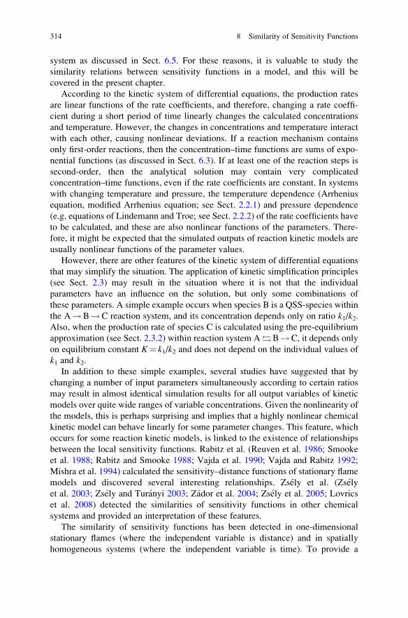
system as discussed in Sect. 6.5. For these reasons, it is valuable to study the

similarity relations between sensitivity functions in a model, and this will be

covered in the present chapter.

According to the kinetic system of differential equations, the production rates

are linear functions of the rate coefficients, and therefore, changing a rate coeffi-

cient during a short period of time linearly changes the calculated concentrations

and temperature. However, the changes in concentrations and temperature interact

with each other, causing nonlinear deviations. If a reaction mechanism contains

only first-order reactions, then the concentration–time functions are sums of expo-

nential functions (as discussed in Sect. 6.3). If at least one of the reaction steps is

second-order, then the analytical solution may contain very complicated

concentration–time functions, even if the rate coefficients are constant. In systems

with changing temperature and pressure, the temperature dependence (Arrhenius

equation, modified Arrhenius equation; see Sect. 2.2.1) and pressure dependence

(e.g. equations of Lindemann and Troe; see Sect. 2.2.2) of the rate coefficients have

to be calculated, and these are also nonlinear functions of the parameters. There-

fore, it might be expected that the simulated outputs of reaction kinetic models are

usually nonlinear functions of the parameter values.

However, there are other features of the kinetic system of differential equations

that may simplify the situation. The application of kinetic simplification principles

(see Sect. 2.3) may result in the situation where it is not that the individual

parameters have an influence on the solution, but only some combinations of

these parameters. A simple example occurs when species B is a QSS-species within

the A!B!C reaction system, and its concentration depends only on ratio k1/k2.Also, when the production rate of species C is calculated using the pre-equilibrium

approximation (see Sect. 2.3.2) within reaction system AÆB!C, it depends only

on equilibrium constant K¼ k1/k2 and does not depend on the individual values of

k1 and k2.In addition to these simple examples, several studies have suggested that by

changing a number of input parameters simultaneously according to certain ratios

may result in almost identical simulation results for all output variables of kinetic

models over quite wide ranges of variable concentrations. Given the nonlinearity of

the models, this is perhaps surprising and implies that a highly nonlinear chemical

kinetic model can behave linearly for some parameter changes. This feature, which

occurs for some reaction kinetic models, is linked to the existence of relationships

between the local sensitivity functions. Rabitz et al. (Reuven et al. 1986; Smooke

et al. 1988; Rabitz and Smooke 1988; Vajda et al. 1990; Vajda and Rabitz 1992;

Mishra et al. 1994) calculated the sensitivity–distance functions of stationary flame

models and discovered several interesting relationships. Zsely et al. (Zsely

et al. 2003; Zsely and Turanyi 2003; Zador et al. 2004; Zsely et al. 2005; Lovrics

et al. 2008) detected the similarities of sensitivity functions in other chemical

systems and provided an interpretation of these features.

The similarity of sensitivity functions has been detected in one-dimensional

stationary flames (where the independent variable is distance) and in spatially

homogeneous systems (where the independent variable is time). To provide a

314 8 Similarity of Sensitivity Functions







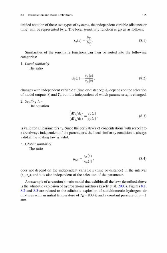
unified notation of these two types of systems, the independent variable (distance or

time) will be represented by z. The local sensitivity function is given as follows:

sij zð Þ ¼ ∂yi∂xj

: ð8:1Þ

Similarities of the sensitivity functions can then be sorted into the following

categories:

1. Local similarityThe ratio

λij zð Þ ¼ sik zð Þsjk zð Þ ; ð8:2Þ

changes with independent variable z (time or distance); λij depends on the selectionof model outputs Yi and Yj, but it is independent of which parameter xk is changed.

2. Scaling lawThe equation

dYi=dzð ÞdYj=dz� � ¼ sik zð Þ

sjk zð Þ ; ð8:3Þ

is valid for all parameters xk. Since the derivatives of concentrations with respect toz are always independent of the parameters, the local similarity condition is always

valid if the scaling law is valid.

3. Global similarityThe ratio

μkm ¼ sik zð Þsim zð Þ ; ð8:4Þ

does not depend on the independent variable z (time or distance) in the interval

(z1, z2), and it is also independent of the selection of the parameter.

An example of a reaction kinetic model that exhibits all the laws described above

is the adiabatic explosion of hydrogen–air mixtures (Zsely et al. 2003). Figures 8.1,

8.2 and 8.3 are related to the adiabatic explosion of stoichiometric hydrogen–air

mixtures with an initial temperature of T0¼ 800 K and a constant pressure of p¼ 1

atm.

8.1 Introduction and Basic Definitions 315

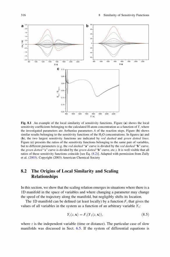
8.2 The Origins of Local Similarity and Scaling

Relationships

In this section, we show that the scaling relation emerges in situations where there is a

1D manifold in the space of variables and where changing a parameter may change

the speed of the trajectory along the manifold, but negligibly shifts its location.

The 1D manifold can be defined (at least locally) by a function Fi that gives the

values of all variables in the system as a function of an arbitrary variable Y1:

Yi z; xð Þ ¼ Fi Y1 z; xð Þð Þ; ð8:5Þ

where z is the independent variable (time or distance). The particular case of slow

manifolds was discussed in Sect. 6.5. If the system of differential equations is

Fig. 8.1 An example of the local similarity of sensitivity functions. Figure (a) shows the local

sensitivity coefficients belonging to the calculated H-atom concentration as a function of T, wherethe investigated parameters are Arrhenius parameters A of the reaction steps. Figure (b) shows

similar results belonging to the sensitivity functions of the H2O concentrations. In figures (a) and

(b), the two largest sensitivity functions are indicated by red dashed and green dotted lines.Figure (c) presents the ratios of the sensitivity functions belonging to the same pair of variables,

but to different parameters (e.g. the red dashed “a” curve is divided by the red dashed “b” curve,

the green dotted “a” curve is divided by the green dotted “b” curve, etc.). It is well visible that allratios of these sensitivity functions coincide [see Eq. (8.2)]. Adapted with permission from Zsely

et al. (2003). Copyright (2003) American Chemical Society



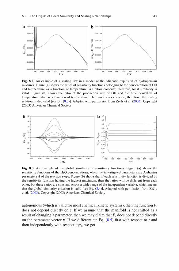
autonomous (which is valid for most chemical kinetic systems), then the function Fi

does not depend directly on z. If we assume that the manifold is not shifted as a

result of changing a parameter, then we may claim that Fi does not depend directly

on the parameter vector x. If we differentiate Eq. (8.5) first with respect to z andthen independently with respect topk, we get

Fig. 8.2 An example of a scaling law in a model of the adiabatic explosion of hydrogen–air

mixtures. Figure (a) shows the ratios of sensitivity functions belonging to the concentration of OH

and temperature as a function of temperature. All ratios coincide; therefore, local similarity is

valid. Figure (b) shows the ratio of the production rate of OH and the time derivative of

temperature, also as a function of temperature. The two curves coincide; therefore, the scaling

relation is also valid [see Eq. (8.3)]. Adapted with permission from Zsely et al. (2003). Copyright

(2003) American Chemical Society

Fig. 8.3 An example of the global similarity of sensitivity functions. Figure (a) shows the

sensitivity functions of the H2O concentrations, when the investigated parameters are Arrhenius

parameters A of the reaction steps. Figure (b) shows that if each sensitivity function is divided by

the sensitivity function having the highest maximum, then the ratios will be different from each

other, but these ratios are constant across a wide range of the independent variable, which means

that the global similarity criterion is valid [see Eq. (8.4)]. Adapted with permission from Zsely

et al. (2003). Copyright (2003) American Chemical Society

8.2 The Origins of Local Similarity and Scaling Relationships 317

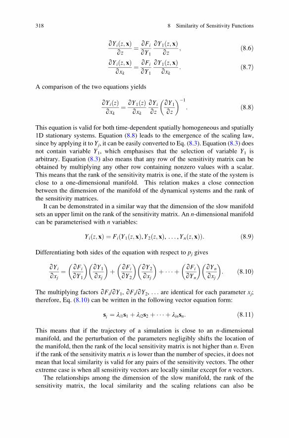
∂Yi z; xð Þ∂z

¼ ∂Fi

∂Y1

∂Y1 z; xð Þ∂z

; ð8:6Þ

∂Yi z; xð Þ∂xk

¼ ∂Fi

∂Y1

∂Y1 z; xð Þ∂xk

: ð8:7Þ

A comparison of the two equations yields

∂Yi zð Þ∂xk

¼ ∂Y1 zð Þ∂xk

∂Yi

∂z∂Y1

∂z

� ��1

: ð8:8Þ

This equation is valid for both time-dependent spatially homogeneous and spatially

1D stationary systems. Equation (8.8) leads to the emergence of the scaling law,

since by applying it to Yj, it can be easily converted to Eq. (8.3). Equation (8.3) doesnot contain variable Y1, which emphasises that the selection of variable Y1 is

arbitrary. Equation (8.3) also means that any row of the sensitivity matrix can be

obtained by multiplying any other row containing nonzero values with a scalar.

This means that the rank of the sensitivity matrix is one, if the state of the system is

close to a one-dimensional manifold. This relation makes a close connection

between the dimension of the manifold of the dynamical systems and the rank of

the sensitivity matrices.

It can be demonstrated in a similar way that the dimension of the slow manifold

sets an upper limit on the rank of the sensitivity matrix. An n-dimensional manifold

can be parameterised with n variables:

Yi z; xð Þ ¼ Fi Y1 z; xð Þ,Y2 z; xð Þ, . . . ,Yn z; xð Þð Þ: ð8:9Þ

Differentiating both sides of the equation with respect to pj gives

∂Yi

∂xj¼ ∂Fi

∂Y1

� �∂Y1

∂xj

� �þ ∂Fi

∂Y2

� �∂Y2

∂xj

� �þ � � � þ ∂Fi

∂Yn

� �∂Yn

∂xj

� �: ð8:10Þ

The multiplying factors ∂Fi/∂Y1, ∂Fi/∂Y2, . . . are identical for each parameter xj;therefore, Eq. (8.10) can be written in the following vector equation form:

si ¼ λi1s1 þ λi2s2 þ � � � þ λinsn: ð8:11Þ

This means that if the trajectory of a simulation is close to an n-dimensional

manifold, and the perturbation of the parameters negligibly shifts the location of

the manifold, then the rank of the local sensitivity matrix is not higher than n. Evenif the rank of the sensitivity matrix n is lower than the number of species, it does not

mean that local similarity is valid for any pairs of the sensitivity vectors. The other

extreme case is when all sensitivity vectors are locally similar except for n vectors.The relationships among the dimension of the slow manifold, the rank of the

sensitivity matrix, the local similarity and the scaling relations can also be


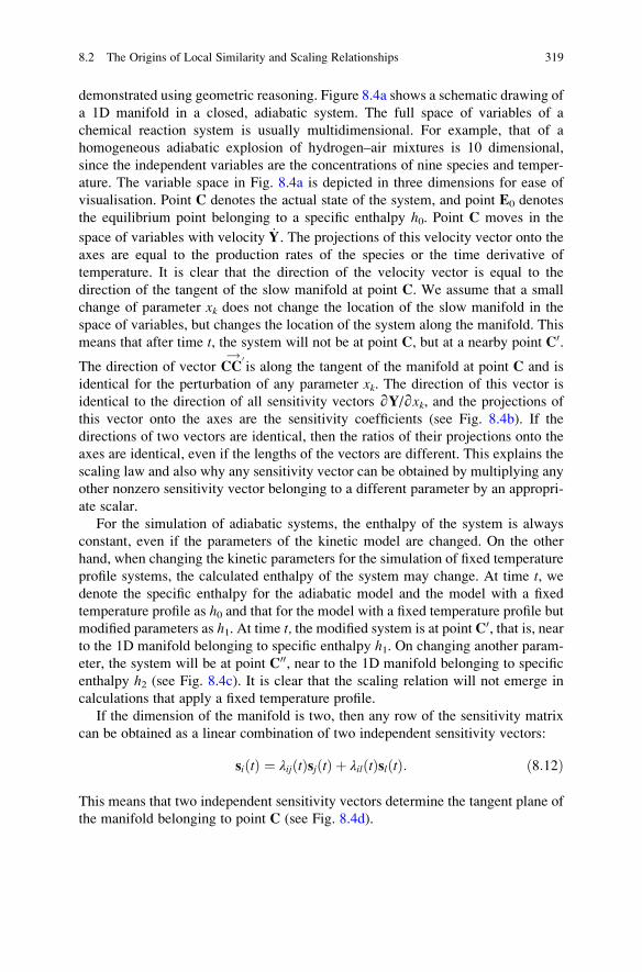
demonstrated using geometric reasoning. Figure 8.4a shows a schematic drawing of

a 1D manifold in a closed, adiabatic system. The full space of variables of a

chemical reaction system is usually multidimensional. For example, that of a

homogeneous adiabatic explosion of hydrogen–air mixtures is 10 dimensional,

since the independent variables are the concentrations of nine species and temper-

ature. The variable space in Fig. 8.4a is depicted in three dimensions for ease of

visualisation. Point C denotes the actual state of the system, and point E0 denotes

the equilibrium point belonging to a specific enthalpy h0. Point C moves in the

space of variables with velocity _Y. The projections of this velocity vector onto the

axes are equal to the production rates of the species or the time derivative of

temperature. It is clear that the direction of the velocity vector is equal to the

direction of the tangent of the slow manifold at point C. We assume that a small

change of parameter xk does not change the location of the slow manifold in the

space of variables, but changes the location of the system along the manifold. This

means that after time t, the system will not be at point C, but at a nearby point C0.

The direction of vector CC0!is along the tangent of the manifold at point C and is

identical for the perturbation of any parameter xk. The direction of this vector is

identical to the direction of all sensitivity vectors ∂Y/∂xk, and the projections of

this vector onto the axes are the sensitivity coefficients (see Fig. 8.4b). If the

directions of two vectors are identical, then the ratios of their projections onto the

axes are identical, even if the lengths of the vectors are different. This explains the

scaling law and also why any sensitivity vector can be obtained by multiplying any

other nonzero sensitivity vector belonging to a different parameter by an appropri-

ate scalar.

For the simulation of adiabatic systems, the enthalpy of the system is always

constant, even if the parameters of the kinetic model are changed. On the other

hand, when changing the kinetic parameters for the simulation of fixed temperature

profile systems, the calculated enthalpy of the system may change. At time t, wedenote the specific enthalpy for the adiabatic model and the model with a fixed

temperature profile as h0 and that for the model with a fixed temperature profile but

modified parameters as h1. At time t, the modified system is at point C0, that is, nearto the 1D manifold belonging to specific enthalpy h1. On changing another param-

eter, the system will be at point C00, near to the 1D manifold belonging to specific

enthalpy h2 (see Fig. 8.4c). It is clear that the scaling relation will not emerge in

calculations that apply a fixed temperature profile.

If the dimension of the manifold is two, then any row of the sensitivity matrix

can be obtained as a linear combination of two independent sensitivity vectors:

si tð Þ ¼ λij tð Þsj tð Þ þ λil tð Þsl tð Þ: ð8:12Þ

This means that two independent sensitivity vectors determine the tangent plane of

the manifold belonging to point C (see Fig. 8.4d).


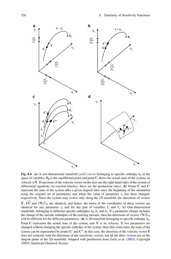
Fig. 8.4 (a) A one-dimensional manifold (solid curve) belonging to specific enthalpy h0 in the

space of variables. E0 is the equilibrium point and point C shows the actual state of the system; its

velocity is _Y. Projections of the velocity vector on the axes are the right-hand sides of the system of

differential equations (in reaction kinetics, these are the production rates). (b) Points C and C0

represent the state of the system after a given elapsed time since the beginning of the simulation

using the original set of parameters and when the value of parameter xk has been changed,

respectively. Since the system may evolve only along the 1D manifold, the directions of vectors

_Y, CC0!and ∂Y/∂xk are identical, and hence, the ratios of the coordinates of these vectors are

identical for any parameter xk and for any pair of variables Yi and Yj. (c) One-dimensional

manifolds, belonging to different specific enthalpies h0, h1 and h2. If a parameter change includes

the change of the specific enthalpies of the reacting mixture, then the directions of vectors ∂Y/∂xkwill be different for the different parameters. (d) A 2D manifold belonging to specific enthalpy h0.

Point C represents the actual state of the system, and _Y is its velocity. If two parameters are

changed without changing the specific enthalpy of the system, then after some time, the state of the

system can be represented by points C0 and C00. In this case, the direction of the velocity vector _Ydoes not coincide with the directions of the sensitivity vectors, but all the three vectors are on the

tangent plane of the 2D manifold. Adapted with permission from Zsely et al. (2003). Copyright

(2003) American Chemical Society


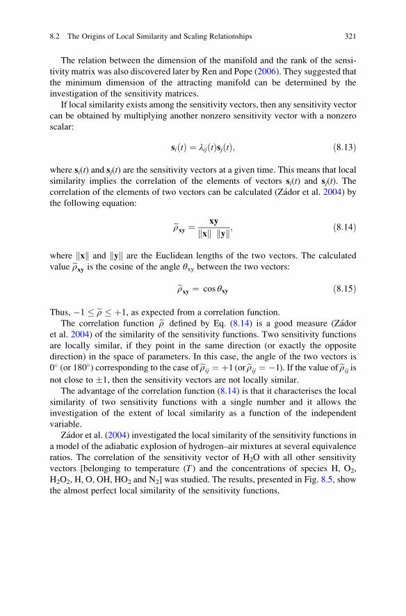
The relation between the dimension of the manifold and the rank of the sensi-

tivity matrix was also discovered later by Ren and Pope (2006). They suggested that

the minimum dimension of the attracting manifold can be determined by the

investigation of the sensitivity matrices.

If local similarity exists among the sensitivity vectors, then any sensitivity vector

can be obtained by multiplying another nonzero sensitivity vector with a nonzero

scalar:

si tð Þ ¼ λij tð Þsj tð Þ; ð8:13Þ

where si(t) and sj(t) are the sensitivity vectors at a given time. This means that local

similarity implies the correlation of the elements of vectors si(t) and sj(t). Thecorrelation of the elements of two vectors can be calculated (Zador et al. 2004) by

the following equation:

eρxy ¼ xy

xk k yk k; ð8:14Þ

where kxk and kyk are the Euclidean lengths of the two vectors. The calculated

value eρxy is the cosine of the angle θxy between the two vectors:

eρxy ¼ cos θxy ð8:15Þ

Thus, �1 � eρ � þ1, as expected from a correlation function.

The correlation function eρ defined by Eq. (8.14) is a good measure (Zador

et al. 2004) of the similarity of the sensitivity functions. Two sensitivity functions

are locally similar, if they point in the same direction (or exactly the opposite

direction) in the space of parameters. In this case, the angle of the two vectors is

0� (or 180�) corresponding to the case ofeρij ¼ þ1 (oreρij ¼ �1). If the value ofeρij isnot close to �1, then the sensitivity vectors are not locally similar.

The advantage of the correlation function (8.14) is that it characterises the local

similarity of two sensitivity functions with a single number and it allows the

investigation of the extent of local similarity as a function of the independent

variable.

Zador et al. (2004) investigated the local similarity of the sensitivity functions in

a model of the adiabatic explosion of hydrogen–air mixtures at several equivalence

ratios. The correlation of the sensitivity vector of H2O with all other sensitivity

vectors [belonging to temperature (T ) and the concentrations of species H, O2,

H2O2, H, O, OH, HO2 and N2] was studied. The results, presented in Fig. 8.5, show

the almost perfect local similarity of the sensitivity functions.


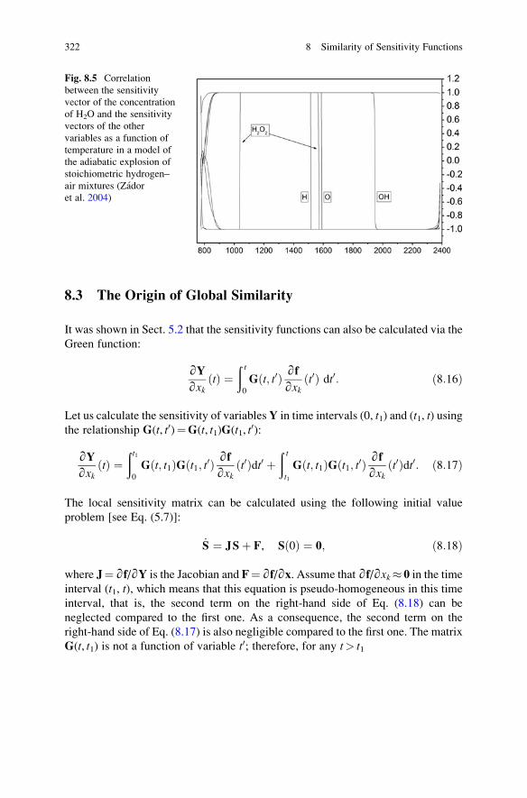
8.3 The Origin of Global Similarity

It was shown in Sect. 5.2 that the sensitivity functions can also be calculated via the

Green function:

∂Y∂xk

tð Þ ¼ð t

0

G t; t0ð Þ ∂f∂xk

t0ð Þ dt0: ð8:16Þ

Let us calculate the sensitivity of variablesY in time intervals (0, t1) and (t1, t) usingthe relationship G(t, t0)¼G(t, t1)G(t1, t

0):

∂Y∂xk

tð Þ ¼ðt10

G t; t1ð ÞG t1; t0ð Þ ∂f∂xk

t0ð Þdt0 þð t

t1

G t; t1ð ÞG t1; t0ð Þ ∂f∂xk

t0ð Þdt0: ð8:17Þ

The local sensitivity matrix can be calculated using the following initial value

problem [see Eq. (5.7)]:

_S ¼ JSþ F, S 0ð Þ ¼ 0; ð8:18Þ

where J¼∂f/∂Y is the Jacobian and F¼∂f/∂x. Assume that ∂f/∂xk� 0 in the time

interval (t1, t), which means that this equation is pseudo-homogeneous in this time

interval, that is, the second term on the right-hand side of Eq. (8.18) can be

neglected compared to the first one. As a consequence, the second term on the

right-hand side of Eq. (8.17) is also negligible compared to the first one. The matrix

G(t, t1) is not a function of variable t0; therefore, for any t> t1

Fig. 8.5 Correlation

between the sensitivity

vector of the concentration

of H2O and the sensitivity

vectors of the other

variables as a function of

temperature in a model of

the adiabatic explosion of

stoichiometric hydrogen–

air mixtures (Zador

et al. 2004)



∂Y∂xk

tð Þ ¼ G t; t1ð Þðt10

G t1; t0ð Þ ∂f∂xk

t0ð Þdt0 ¼ G t; t1ð Þ ∂Y∂xk

t1ð Þ: ð8:19Þ

The sensitivity of variable Yi with respect to parameter xk can be calculated in the

following way:

∂Yi

∂xktð Þ ¼

XNj¼1

gij t; t1ð Þ∂Yj

∂xkt1ð Þ: ð8:20Þ

If the sensitivity functions are locally similar at time t1, then the ratios of any two

sensitivity coefficients are independent of the selection of the modified parameter.

Let us select another variable Yh and substitute Eq. (8.2) that defines the local

similarity into Eq. (8.20):

∂Yi

∂xktð Þ ¼ ∂Yh

∂xkt1ð Þ

XNj¼1

gij t; t1ð Þλjh t1ð Þ; ð8:21Þ

∂Yi

∂xktð Þ

� �=

∂Yh

∂xkt1ð Þ

� �¼

XNj¼1

gij t; t1ð Þλjh t1ð Þ: ð8:22Þ

A similar equation can be obtained for parameter xm:

∂Yi

∂xmtð Þ

� �=

∂Yh

∂xmt1ð Þ

� �¼

XNj¼1

gij t; t1ð Þλjh t1ð Þ: ð8:23Þ

The right-hand sides of Eqs. (8.22) and (8.23) are identical, and the combination of

these two equations yields

∂Yi

∂xktð Þ

∂Yi

∂xmtð Þ ¼

∂Yh

∂xkt1ð Þ

∂Yh

∂xmt1ð Þ ¼ μkm: ð8:24Þ

Equation (8.24) shows that the ratio of two sensitivity coefficients at any time

t> t1 is independent of the selection of the model result Yi and time. Therefore, the

corresponding sensitivity functions are globally similar. The meaning of Eqs. (8.16)

to (8.24) can be summarised as follows. If the sensitivity differential equations are

pseudo-homogeneous in the time interval (t1, t2) and the sensitivity coefficients are

locally similar at time t1, then the sensitivity functions are globally similar in the

time interval (t1, t2). The ratio μkm is independent of the selection of model output Yiand therefore Eq. (8.21) implies the presence of global and local similarity at the

same time.

8.3 The Origin of Global Similarity 323

The proof above is based on the derivation of Vajda and Rabitz (1992), which

was generalised by Zsely et al. (2003) for an arbitrary number of variables. The

main difference between the two derivations is that Vajda and Rabitz assumed that

one of the variables is dominant. If variable Yh is dominant, then

gih t; t1ð Þ∂Yh

∂xkt1ð Þ �

XNþ1

j¼1, j6¼h

gij t; t1ð Þ∂Yj


This means that all terms but the one belonging to the dominant variable can be

neglected in Eq. (8.16):

∂Yi

∂xktð Þ ¼ gih t; t1ð Þ∂Yh


If the derivation is also applied for parameter xm, then the combination of the two

equations yields again Eq. (8.21):

∂Yi

∂xktð Þ

∂Yi

∂xmtð Þ ¼

∂Yh

∂xkt1ð Þ

∂Yh

∂xmt1ð Þ ¼ μkm: ð8:27Þ

Thus, the result of this derivation is identical to the previous one.

According to the reasoning in Zsely et al. (2003), if in the time interval (t1, t2),the system of sensitivity differential equations is pseudo-homogeneous and local

similarity is present, then the sensitivity functions are globally similar. According

to the derivation of Vajda and Rabitz (1992), if in the time interval (t1, t2) the systemof sensitivity differential equations is pseudo-homogeneous and one of the vari-

ables is dominant, then the sensitivity functions are locally and globally similar.

Vajda and Rabitz considered that temperature is a dominant variable in ignition

systems. Zsely et al. (2003) investigated the reason behind the global similarity of

sensitivity functions for simulations of the adiabatic explosion of hydrogen–air

mixtures. Figure 8.6 shows that in the region of global similarity, the inhomo-

geneous term of the sensitivity differential equation is negligible compared to the

homogeneous term. That means that the sensitivity system of differential equations

(8.18) is pseudo-homogeneous. They also demonstrated that in this system, none of

the variables are dominant.

Derivation of the condition of global similarity for spatially one-dimensional,

stationary systems is similar, but not identical. Due to causality, in temporal

systems, parameter changes affect only later events. In 1D reaction–diffusion

systems, a parameter change may modify the concentrations in both spatial direc-

tions. The adaption of the derivation above to reaction–diffusion systems is

discussed in the article of Zsely et al. (2003).


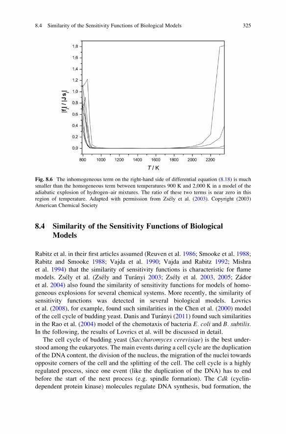
8.4 Similarity of the Sensitivity Functions of Biological

Models

Rabitz et al. in their first articles assumed (Reuven et al. 1986; Smooke et al. 1988;

Rabitz and Smooke 1988; Vajda et al. 1990; Vajda and Rabitz 1992; Mishra

et al. 1994) that the similarity of sensitivity functions is characteristic for flame

models. Zsely et al. (Zsely and Turanyi 2003; Zsely et al. 2003, 2005; Zador

et al. 2004) also found the similarity of sensitivity functions for models of homo-

geneous explosions for several chemical systems. More recently, the similarity of

sensitivity functions was detected in several biological models. Lovrics

et al. (2008), for example, found such similarities in the Chen et al. (2000) model

of the cell cycle of budding yeast. Danis and Turanyi (2011) found such similarities

in the Rao et al. (2004) model of the chemotaxis of bacteria E. coli and B. subtilis.In the following, the results of Lovrics et al. will be discussed in detail.

The cell cycle of budding yeast (Saccharomyces cerevisiae) is the best under-

stood among the eukaryotes. The main events during a cell cycle are the duplication

of the DNA content, the division of the nucleus, the migration of the nuclei towards

opposite corners of the cell and the splitting of the cell. The cell cycle is a highly

regulated process, since one event (like the duplication of the DNA) has to end

before the start of the next process (e.g. spindle formation). The Cdk (cyclin-

dependent protein kinase) molecules regulate DNA synthesis, bud formation, the

Fig. 8.6 The inhomogeneous term on the right-hand side of differential equation (8.18) is much

smaller than the homogeneous term between temperatures 900 K and 2,000 K in a model of the

adiabatic explosion of hydrogen–air mixtures. The ratio of these two terms is near zero in this

region of temperature. Adapted with permission from Zsely et al. (2003). Copyright (2003)

American Chemical Society

8.4 Similarity of the Sensitivity Functions of Biological Models 325

separation of the nucleus and the separation of the cells. At first, the new cell is just

growing (phase G1), and the next phase is DNA synthesis (phase S/G2). Finally,

two identical nuclei and then two new cells are formed (mitosis, phase M).

The Chen model of the budding yeast cell cycle (Chen et al. 2000) consists of a

system of ordinary differential equations with 13 variables and coupled algebraic

equations. One of the variables is the mass of the cell that increases exponentially

between two cell divisions. Three of the variables define the state of the cell, whilst

the other nine variables are the concentrations of nine proteins. The Chen model is

basically a reaction kinetic model, since the core of the model describes the

synthesis and interactions of proteins. The model has 73 parameters.

Lovrics et al. (2006) carried out a timescale and dimension analysis of the Chen

model as presented in Fig. 6.8. The cell mass continuously grows, and therefore,

one of the real parts of the eigenvalues Re(λi) of the Jacobian is always positive. Theother Re(λi) eigenvalues are usually negative, except for during certain time

domains of the cell cycle. If at least one of the other Re(λi) eigenvalues is positive(the time domain is indicated by the grey shading in Fig. 6.8), then the dynamical

dimension of the model is increasing; otherwise, it is decreasing. Lovrics

et al. (2006) gave a detailed explanation as to the biological background of these

grey excitation periods.

Timescale and dimension analysis revealed that during several time domains of

the cell cycle, the dynamic dimension of the model is low and that during the cell

cycle excitation and relaxation periods, it alternates between higher and lower

dimensions. According to Sect. 8.3, these two features together may trigger the

global similarity of the sensitivity functions. Therefore, Lovrics et al. investigated

the sensitivity functions of the Chen model (2008) .

Figure 8.7 shows the sensitivity functions of the concentration of protein Cln2during a full cycle. Similar functions were obtained for the sensitivity functions of

all other variables. It is clear that the sensitivity functions of Cln2 usually increase

in the excitation (grey) periods. The reason is that a parameter change after a certain

time causes a shift in the values of variables, and this shift becomes amplified, thus

increasing the sensitivity functions. In the relaxation (white) periods, all Re(λi)eigenvalues are negative; therefore, the difference between the original and the

perturbed solution decreases and the sensitivity functions tend to zero.

Figure 8.7 demonstrates that the shapes of some sensitivity functions are similar

to those of others. Obviously, several groups of sensitivity functions can be

separated so that each group contains functions of a similar shape. Within each

group, any sensitivity function can be obtained by multiplying any other function

by a positive or negative scalar, that is, the sensitivity functions are globally similar.

The sensitivity functions were sorted in the following way. First, each function

was divided by its maximum with the result that similar functions almost coincided.

Figure 8.8 shows such normalised sensitivity functions for the species Cln2. It isclear that most of the functions follow either the shape indicated by the solid line

(“shape A”) or that indicated by the dotted line (“shape B”). For the model

simulating the explosion of hydrogen–air mixtures, all sensitivity functions were




Fig. 8.7 Sensitivity functions of enzyme Cln2 (Lovrics et al. 2008). The excitation periods are

denoted by grey shading. Time zero is the time of cell division. The sensitivity functions are

labelled with the names of the parameters; these parameter names are identified in the article of

Chen et al. (2000)

Fig. 8.8 Sensitivity functions of enzyme Cln2 normalised to unit maximum. The thick solid lineindicates 10 coinciding functions having shape A, whilst the dotted line shows 38 coinciding

functions having shape B. The shapes of other 9 sensitivity functions (thin solid line) are not

similar to either shapes A or B (Lovrics et al. 2008)


globally similar. On the other hand, for the cell cycle model, most of the sensitivity

functions can be sorted into one of the two groups, but several functions do not

follow either of these two shapes.

Similar sorting of all 73 sensitivity functions belonging to each of the 13 vari-

ables was automated using cluster analysis. The shapes of the sensitivity functions

were investigated between two cell divisions, that is, in the time interval [t1, t2]. Asdiscussed above, the sensitivity functions were normalised first to unit maximum:

s_ik tð Þ ¼ sik tð Þ=max sik tð Þj j: ð8:28Þ

Next, the integral of the square of the difference of two sensitivity functions was

calculated during the interval [t1, t2]. Mathematically speaking, the L2 distance of

the normalised sensitivity functions was calculated:

Ci k; lð Þ ¼ðt2t1

s_ik tð Þ � s

_il tð Þ

� �2

dt; ð8:29Þ

Ci(k, l ) is a non-negative value that shows the distance of the shapes of two

sensitivity functions belonging to variable i and parameters k and l. If there is a

perfect global similarity between the two sensitivity functions, then Ci(k, l )¼ 0.

Non-similar sensitivity functions are related to large Ci(k, l ) values. Values of

Ci(k, l ) can be arranged into a matrix Ci, and this distance matrix can be investi-

gated using cluster analysis.

Cluster analysis (Everitt et al. 2001) is a tool for grouping various objects on thebasis of their distance in a multidimensional space. In chemistry, cluster analysis is

used for the interpretation of analytical results. For example, in food or drink

samples, the concentrations of many chemicals are measured, and the question is

which of the samples are similar on the basis of the analytical results. The first step

is always the transformation of the raw measurement data into a distance matrix.

The general features of a distance matrix are that the diagonal elements are zero

(everything is at zero distance from itself), all matrix elements are non-negative

(negative distance cannot be interpreted) and the matrix is symmetrical (to and from

distances are identical). It is clear that the distance matrix defined by Eq. (8.29)

fulfils these requirements.

One of the cluster analysis methods is the agglomerative method (Everitt

et al. 2001). Using this approach, a distance threshold parameter is continuously

increased. At the first step, the two nearest objects are identified, and at this stage,

only their distance is below the threshold. These two objects are united and the

location of the unified object is the arithmetic mean of the coordinates. By increas-

ing the threshold further and further, objects are united until only one object

remains. The similarity of the objects is indicated by the order of the aggregations.


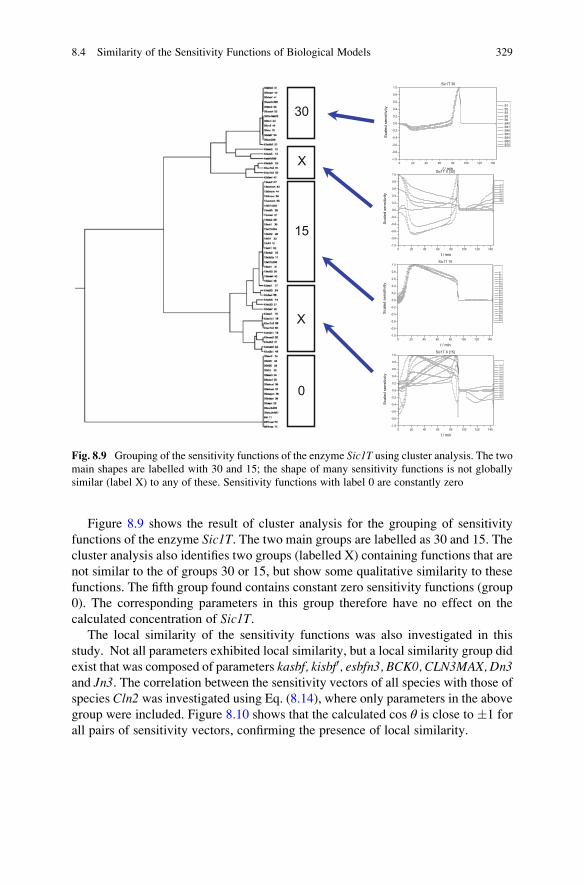
Figure 8.9 shows the result of cluster analysis for the grouping of sensitivity

functions of the enzyme Sic1T. The two main groups are labelled as 30 and 15. The

cluster analysis also identifies two groups (labelled X) containing functions that are

not similar to the of groups 30 or 15, but show some qualitative similarity to these

functions. The fifth group found contains constant zero sensitivity functions (group

0). The corresponding parameters in this group therefore have no effect on the

calculated concentration of Sic1T.The local similarity of the sensitivity functions was also investigated in this

study. Not all parameters exhibited local similarity, but a local similarity group did

exist that was composed of parameters kasbf, kisbf0, esbfn3, BCK0, CLN3MAX, Dn3and Jn3. The correlation between the sensitivity vectors of all species with those ofspecies Cln2 was investigated using Eq. (8.14), where only parameters in the above

group were included. Figure 8.10 shows that the calculated cos θ is close to �1 for

all pairs of sensitivity vectors, confirming the presence of local similarity.

0 20 40 60 80 100 120 140-1.0

-0.8

-0.6

-0.4

-0.2

0.0

0.2

0.4

0.6

0.8

1.0Sic1T X [15]

Sca

led

sens

itivi

ty

t / min

B14B16B17B18B19B20B22B24B27B42B49B58B59B60B21

30

X

15

X

0

0 20 40 60 80 100 120 140-1.0

-0.8

-0.6

-0.4

-0.2

0.0

0.2

0.4

0.6

0.8

1.0Sic1T 15

Sca

led

sens

itivi

ty

t / min

B7B8B9B10B11B25B26B30B31B33B43B44B45B46B50B51B55B56B57B63B64B65

0 20 40 60 80 100 120 140-1.0

-0.8

-0.6

-0.4

-0.2

0.0

0.2

0.4

0.6

0.8

1.0

Sca

led

sens

itivi

ty

t / min

B1B2B3B5B6B40B41B48B53B54B68B70

Sic1T 30

0 20 40 60 80 100 120 140-1.0

-0.8

-0.6

-0.4

-0.2

0.0

0.2

0.4

0.6

0.8

1.0Sic1T X [30]

Sca

led

sens

itivi

ty

t / min

B12B13B15B47B61B62B23B69

Fig. 8.9 Grouping of the sensitivity functions of the enzyme Sic1T using cluster analysis. The two

main shapes are labelled with 30 and 15; the shape of many sensitivity functions is not globally

similar (label X) to any of these. Sensitivity functions with label 0 are constantly zero


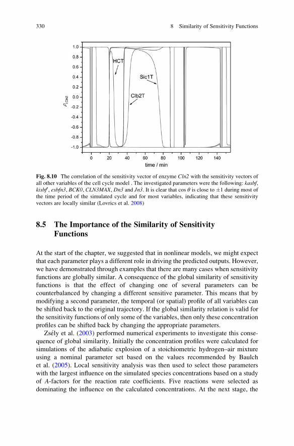
8.5 The Importance of the Similarity of Sensitivity

Functions

At the start of the chapter, we suggested that in nonlinear models, we might expect

that each parameter plays a different role in driving the predicted outputs. However,

we have demonstrated through examples that there are many cases when sensitivity

functions are globally similar. A consequence of the global similarity of sensitivity

functions is that the effect of changing one of several parameters can be

counterbalanced by changing a different sensitive parameter. This means that by

modifying a second parameter, the temporal (or spatial) profile of all variables can

be shifted back to the original trajectory. If the global similarity relation is valid for

the sensitivity functions of only some of the variables, then only these concentration

profiles can be shifted back by changing the appropriate parameters.

Zsely et al. (2003) performed numerical experiments to investigate this conse-

quence of global similarity. Initially the concentration profiles were calculated for

simulations of the adiabatic explosion of a stoichiometric hydrogen–air mixture

using a nominal parameter set based on the values recommended by Baulch

et al. (2005). Local sensitivity analysis was then used to select those parameters

with the largest influence on the simulated species concentrations based on a study

of A-factors for the reaction rate coefficients. Five reactions were selected as

dominating the influence on the calculated concentrations. At the next stage, the

Fig. 8.10 The correlation of the sensitivity vector of enzyme Cln2 with the sensitivity vectors of

all other variables of the cell cycle model . The investigated parameters were the following: kasbf,kisbf0, esbfn3, BCK0, CLN3MAX, Dn3 and Jn3. It is clear that cos θ is close to �1 during most of

the time period of the simulated cycle and for most variables, indicating that these sensitivity

vectors are locally similar (Lovrics et al. 2008)


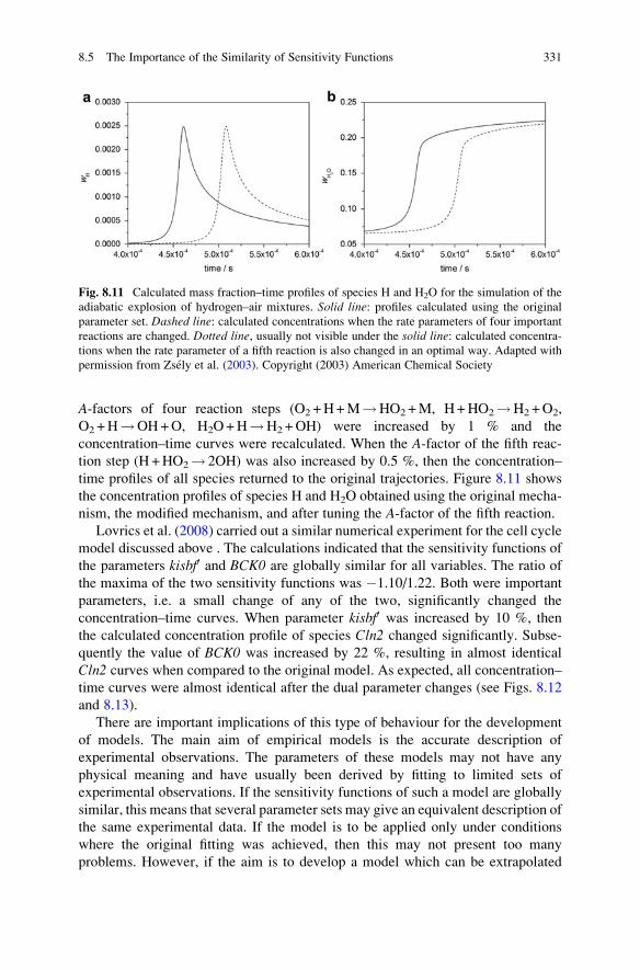
A-factors of four reaction steps (O2 +H+M!HO2+M, H+HO2!H2+O2,

O2 +H!OH+O, H2O+H!H2+OH) were increased by 1 % and the

concentration–time curves were recalculated. When the A-factor of the fifth reac-

tion step (H +HO2! 2OH) was also increased by 0.5 %, then the concentration–

time profiles of all species returned to the original trajectories. Figure 8.11 shows

the concentration profiles of species H and H2O obtained using the original mecha-

nism, the modified mechanism, and after tuning the A-factor of the fifth reaction.

Lovrics et al. (2008) carried out a similar numerical experiment for the cell cycle

model discussed above . The calculations indicated that the sensitivity functions of

the parameters kisbf0 and BCK0 are globally similar for all variables. The ratio of

the maxima of the two sensitivity functions was �1.10/1.22. Both were important

parameters, i.e. a small change of any of the two, significantly changed the

concentration–time curves. When parameter kisbf0 was increased by 10 %, then

the calculated concentration profile of species Cln2 changed significantly. Subse-

quently the value of BCK0 was increased by 22 %, resulting in almost identical

Cln2 curves when compared to the original model. As expected, all concentration–

time curves were almost identical after the dual parameter changes (see Figs. 8.12

and 8.13).

There are important implications of this type of behaviour for the development

of models. The main aim of empirical models is the accurate description of

experimental observations. The parameters of these models may not have any

physical meaning and have usually been derived by fitting to limited sets of

experimental observations. If the sensitivity functions of such a model are globally

similar, this means that several parameter sets may give an equivalent description of

the same experimental data. If the model is to be applied only under conditions

where the original fitting was achieved, then this may not present too many

problems. However, if the aim is to develop a model which can be extrapolated

Fig. 8.11 Calculated mass fraction–time profiles of species H and H2O for the simulation of the

adiabatic explosion of hydrogen–air mixtures. Solid line: profiles calculated using the original

parameter set. Dashed line: calculated concentrations when the rate parameters of four important

reactions are changed. Dotted line, usually not visible under the solid line: calculated concentra-

tions when the rate parameter of a fifth reaction is also changed in an optimal way. Adapted with

permission from Zsely et al. (2003). Copyright (2003) American Chemical Society

8.5 The Importance of the Similarity of Sensitivity Functions 331

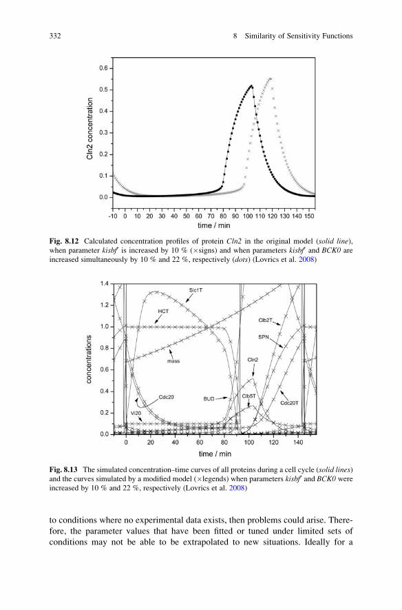
to conditions where no experimental data exists, then problems could arise. There-

fore, the parameter values that have been fitted or tuned under limited sets of

conditions may not be able to be extrapolated to new situations. Ideally for a

Fig. 8.12 Calculated concentration profiles of protein Cln2 in the original model (solid line),when parameter kisbf0 is increased by 10 % (signs) and when parameters kisbf0 and BCK0 are

increased simultaneously by 10 % and 22 %, respectively (dots) (Lovrics et al. 2008)

Fig. 8.13 The simulated concentration–time curves of all proteins during a cell cycle (solid lines)and the curves simulated by a modified model (legends) when parameters kisbf0 and BCK0 wereincreased by 10 % and 22 %, respectively (Lovrics et al. 2008)


model to be general, it should be able to be extrapolated, and therefore, more

physically based approaches to model development are becoming common as

opposed to purely empirical models.

Physical models contain parameters that are developed at a more fundamental

level and are thought to have “real” physical meaning. They are often derived from

different sources, e.g. experimental measurements that attempt to isolate a single

parameter, or theoretical calculations (see Chap. 3). A physical model is usually

considered to be “validated” if the model reproduces all experimental data within

their uncertainty limits across a wide range of values of the independent variables.

Assuming there is perfect agreement between the model simulations and experi-

mental data, we may be tempted to interpret the parameters of the “validated”

model as physically correct values. However, the results of the numerical experi-

ments above show that if one or some of the parameter values in a physical model

are incorrect, this may be disguised by setting other parameters to incorrect values.

If the errors are perfectly balanced, the model may still reproduce all experimental

data quite well. Therefore, it is dangerous to determine rate coefficients within a

complex mechanism, by fitting one or several rate parameters to experimental data,

whilst fixing the other parameters within the model at their literature values, when

in fact these fixed parameters may be uncertain to varying degrees (see Sect. 5.6.1).

Small inaccuracies in the fixed values may result in large deviations in the fitted

values, whilst the model still describes the experimental data well. This could be

one reason why complex chemical kinetic models suggested by different authors

provide descriptions of experimental data with similar accuracy, even though the

applied rate coefficients are very different. Parameters of globally similar sensiti-

vity functions are in a kind of cooperative relationship, since if the value of one

parameter is changed, then its effect can be compensated by an appropriate change

in the other parameter. The identification of such cooperative parameters promotes

a better understanding of the model.

The comments above are valid for all types of models. However, there are some

aspects of the global similarity of sensitivity functions that are especially interesting

and important for biological models. Gutenkunst et al. (2007) highlighted that many

systems biology models have sensitivity coefficients of similar magnitude and

fitting all these parameters simultaneously to the experimental data results in

unrealistically large parameter uncertainties. They investigated 17 published

models and called such sensitivities as “universally sloppy parameter sensitivities”.

Gutenkunst et al. identified that the main reason for this behaviour is that only

parameter groups, and not the individual parameters, influence the model solution

in most systems biology models. Note that such parameter groups can be a result of

global similarity and that these parameter groups can be identified by the principal

component analysis of the local sensitivity matrix (see Sect. 5.3).

A general feature of living organisms is that the error of a part of an organism

can often be compensated for by another part. Evolution has promoted the emer-

gence of such features, and hence, this error-correcting feature of living organisms

is general and is present in the anatomy of several organs (Wagner 2013). Also,

most regulating mechanisms contain parallel pathways. In this way, a failure of one

8.5 The Importance of the Similarity of Sensitivity Functions 333

http://dx.doi.org/10.1007/978-3-662-44562-4_3



pathway can be compensated for by a backup system. There are also similar parallel

pathways in cell cycle regulation, and if one route is eliminated by a mutation, the

other pathways may take over its role. However, this may not account for all error

correction mechanisms.

The global similarity of sensitivity functions indicates the possibility for a novel

error correction mechanism. A change of activity of an important enzyme can be

fully compensated for by the change of activity of another enzyme, thereby

restoring the concentration profiles of important species at all times. This error

correction mechanism can be used not only once, but unlimited times, since later

there are further possibilities for small adjustments. This feature is quantitatively

different to those of other error correction mechanisms when, e.g., backup parallel

pathways are used. The groups of enzymes that can be partners in this process can

be identified by the inspection of the sensitivity functions of detailed chemical

kinetics (systems biology) models of biological systems with implications for the

treatment of disease.

The cause of some diseases is that the parameters of certain chemical reactions

become different from those parameters which are characteristic for a healthy body.

A possible aim of treatment is to restore the original parameters using medical

drugs, but this can be difficult in some cases. However, if parameters which are

globally similar to the original parameters are changed using drug therapy, then

healthy functioning could be restored in a different way. This second option offers

wider possibilities, and the rates of other biological processes can be influenced in

an easier way. Therefore, an emerging trend in the pharmaceutical industry is to

apply drug therapies to fix not the direct cause of the disease, but to restore healthy

functioning in an indirect way. As more and more detailed models are developed for

biological systems, the investigation of similarities in the sensitivity functions may

provide a theoretical background for this new approach to the development of

medical drugs.

The similarity of sensitivity functions may also have a role in genetic error

correction. Let us assume that in a biochemical regulatory system, the protein

concentration profiles have been refined by evolution and are nearly ideal for a

given task. However, errors may occur during DNA replication, for example,

resulting in lower enzyme activity. This error can either be lethal or can result in

damaged functioning of the cell in the surviving organism. In the latter case, a

further mutation may correct the previous error. It is very unlikely that the next

mutation exactly corrects the functioning of the same enzyme. However, if the

sensitivity functions of the regulatory system are globally similar, then within a

group of enzymes, the activity change of any other enzyme may correct the

functioning of the regulation. If a second mutation of this type yields a fit cell, it

is evolutionary advantageous, and therefore, such a correction may remain

permanent.

It is clear from these discussions that the development of detailed models of

biochemical processes and the investigation of their sensitivity relationships may

have important applications in improving our understanding of disease and in

developing treatments. Not surprisingly, therefore, a great detail of effort is being


invested into the development of systems biology models with increasing levels of

detail as discussed in Chap. 3. The types of behaviour indicated by the models

discussed in this chapter indicate that this will be a fruitful area of research.

References




Chen, C.C., Csikasz-Nagy, A., Gyorffy, B., Val, J., Novak, B., Tyson, J.J.: Kinetic analysis of a

molecular model of the budding yeast cell cycle. Mol. Biol. Cell 11, 369–391 (2000)

Danis, J., Turanyi, T.: Sensitivity analysis of bacterial chemotaxis models. Procedia Comput. Sci.

7, 233–234 (2011)

Everitt, B.S., Landau, S., Leese, M.: Cluster Analysis. Oxford University Press, Oxford (2001)

Gutenkunst, R.N., Waterfall, J.J., Casey, F.P., Brown, K.S., Myers, C.R., Sethna, J.P.: Universally

sloppy parameter sensitivities in systems biology models. PLoS Comput. Biol. 3, e189 (2007)

Lovrics, A., Csikasz-Nagy, A., Zsely, I.G., Zador, J., Turanyi, T., Novak, B.: Time scale and

dimension analysis of a budding yeast cell cycle model. BMC Bioinform. 7, 494 (2006)

Lovrics, A., Zsely, I.G., Csikasz-Nagy, A., Zador, J., Turanyi, T., Novak, B.: Analysis of a budding

yeast cell cycle model using the shapes of local sensitivity functions. Int. J. Chem. Kinet. 40,

710–720 (2008)

Mishra, M.K., Yetter, R.A., Reuven, Y., Rabitz, H.: On the role of transport in the combustion

kinetics of a steady-state premixed laminar CO+H2+O2 flame. Int. J. Chem. Kinet. 26, 437–453

(1994)

Rabitz, H., Smooke, M.D.: Scaling relations and self-similarity conditions in strongly coupled

dynamical systems. J. Phys. Chem. 92, 1110–1119 (1988)

Rao, C.V., Frenklach, M., Arkin, A.P.: An allosteric model for transmembrane signaling in

bacterial chemotaxis. J. Mol. Biol. 343, 291–303 (2004)

Ren, Z., Pope, S.B.: The geometry of reaction trajectories and attracting manifolds in composition

space. Combust. Theory Model. 10, 361–388 (2006)

Reuven, Y., Smooke, M.D., Rabitz, H.: Sensitivity analysis of boundary value problems: appli-

cation to nonlinear reaction-diffusion systems. J. Comput. Phys. 64, 27–55 (1986)

Smooke, M.D., Rabitz, H., Reuven, Y., Dryer, F.L.: Application of sensitivity analysis to premixed

hydrogen-air flames. Combust. Sci. Technol. 59, 295–319 (1988)

Vajda, S., Rabitz, H.: Parametric sensitivity and self-similarity in thermal explosion theory. Chem.

Eng. Sci. 47, 1063–1078 (1992)

Vajda, S., Rabitz, H., Yetter, R.A.: Effects of thermal coupling and diffusion on the mechanism of

H2 oxidation in steady premixed laminar flames. Combust. Flame 82, 270–297 (1990)

Wagner, A.: Robustness and Evolvability in Living Systems. Princeton Studies in Complexity.

Princeton University Press, Princeton (2013)

Zador, J., Zsely, I.G., Turanyi, T.: Investigation of the correlation of sensitivity vectors of

hydrogen combustion models. Int. J. Chem. Kinet. 36, 238–252 (2004)

Zsely, I.G., Turanyi, T.: The influence of thermal coupling and diffusion on the importance of

reactions: the case study of hydrogen-air combustion. PCCP 5, 3622–3631 (2003)

Zsely, I.G., Zador, J., Turanyi, T.: Similarity of sensitivity functions of reaction kinetic models.

J. Phys. Chem. A 107, 2216–2238 (2003)



References 335

http://dx.doi.org/10.1007/978-3-662-44562-4_3

Chapter 9

Computer Codes for the Study of ComplexReaction Systems

Abstract This book discusses many complicated algorithms for the investigation

and reduction of simulation models based on detailed reaction mechanisms. Fortu-

nately, computer codes are readily available to facilitate the application of most of

the methods described in this book. A large number of these codes have been made

freely available for teaching and academic research. Many commercial codes

(usually with good support) are also offered for these tasks, and for most commer-

cial codes, academic licences are available at a lower cost than commercial ones. In

this chapter we introduce a range of such computer programs which are organised

according to the following categories: (1) general simulation codes in reaction

kinetics, (2) special codes for the simulation of gas kinetic systems, (3) programs

for the analysis and reduction of reaction mechanisms, (4) programs for the

investigation of biological reaction kinetic systems (“systems biology codes”) and

finally (5) codes for global uncertainty analysis. In all cases the basic features of the

codes are discussed and a reference to the availability is given.

9.1 General Simulation Codes in Reaction Kinetics

WINPP/XPP (WINPP/XPP) is a simulation code that can be used within a Win-

dows or X-Window environment. The code can solve several types of differential

equations, including systems of ODEs, DAEs and also some partial differential

equations. The text input file should contain the differential equation to be solved

and the parameters that control the solution. The program can be used for the

numerical solution of general differential equations without user programming, but

does not provide special support for the simulation of chemical kinetic systems.

Therefore, the user must form the rate equations from the chemical reaction steps

before use. However, WINPP/XPP is popular among biochemical modellers

(Novak et al. 2001; Sedaghat et al. 2002; Fall et al. 2005; Brauer and Castillo-

Chavez 2011).

Based on equations (2.5) and (2.6), it is easy to develop a code that generates the

kinetic system of differential equations on the basis of the chemical reaction steps

and the rate parameters. Starting from the initial concentrations and using a stiff



337

ODE solver, the program calculates the concentration–time curves and provides the

results in the form of tables and graphs. Such a simulation code was developed at

the National Institute of Science and Technology (NIST), called ACUCHEM,

(Braun et al. 1988; ACUCHEM). Other similar simulation codes are Tenua(Tenua) and program DIFF of the KINAL package (Turanyi 1990; KINAL).

The computer code KPP (Damian et al. 2002; Sandu et al. 2003; Daescu

et al. 2003; KPP) is also a simulation program that is specific to chemical kinetics

problems and has been primarily used within the atmospheric chemistry commu-

nity. The code produces the kinetic system of differential equations from the

reaction mechanism by assuming mass action kinetics. The ODEs as well as the

system Jacobian can then be exported in various formats including Fortran77,

Fortran90, C or Matlab. KPP also provides a range of methods for the effective

numerical solution of stiff ODEs including the implementation of sparse matrix

routines. It includes a library containing commonly used atmospheric chemical

reaction mechanisms as well as the facility for users to add to this library. It is also

straightforward to expand the capabilities of the program with new reaction mech-

anisms and new numerical methods. The application of KPP to various problems in

atmospheric chemistry was discussed in Damian et al. (2002), Sandu et al. (2003)

and Daescu et al. (2003).

Reaction kinetics simulation codes usually include subroutines for the solution

of stiff systems of kinetic differential equations and the related ODEs for the

calculation of local sensitivity coefficients. However, the application of the QSSA

frequently results in coupled stiff algebraic–differential equation systems and the

solution of these is a special numerical problem. In libraries of numerical methods,

Fortran and C++ subroutines are available for the solution of coupled stiff

algebraic–differential equation systems [see e.g. NAG Fortran Library D02NGF,

(NAG 2014)] and the package DASSL was mentioned as a commonly used package

in Sect. 7.8.3 (Maly and Petzold 1996). Recently, Matlab has become a widely used

programming language within scientific and engineering computing, and therefore,

such routines have also been made freely available in the SUNDIALS Matlab

program package (SUNDIALS). SUNDIALS is an abbreviation of “SUite of

Nonlinear and DIfferential/ALgebraic equation Solvers”. It allows the application

of computer codes in Matlab that have previously been widely used within the

Fortran environment. Such codes include CVODES (for the solution of stiff ODE

systems and sensitivity analysis), IDAS (solution of initial value problems for DAE

systems and sensitivity analysis) and KINSOL (solution of nonlinear algebraic

systems).

Reaction kinetic models can be simulated not only by solving the kinetic system

of differential equations but also via simulating the equivalent stochastic models.

Computer codes are available that solve the stochastic kinetic equations. One of

these is the Chemical Kinetics Simulator (CKS) program that was developed at

IBM’s Almaden Research Centre. It provides a rapid, interactive method for the

accurate simulation of chemical reactions. CKS is a good tool for teaching the

principles of stochastic reaction kinetics to students and trainees.

338 9 Computer Codes for the Study of Complex Reaction Systems


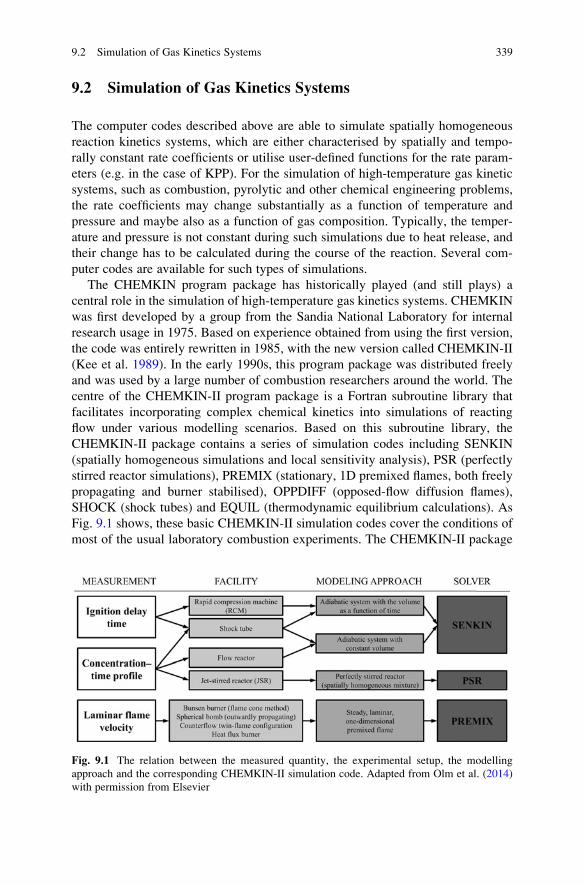
9.2 Simulation of Gas Kinetics Systems

The computer codes described above are able to simulate spatially homogeneous

reaction kinetics systems, which are either characterised by spatially and tempo-

rally constant rate coefficients or utilise user-defined functions for the rate param-

eters (e.g. in the case of KPP). For the simulation of high-temperature gas kinetic

systems, such as combustion, pyrolytic and other chemical engineering problems,

the rate coefficients may change substantially as a function of temperature and

pressure and maybe also as a function of gas composition. Typically, the temper-

ature and pressure is not constant during such simulations due to heat release, and

their change has to be calculated during the course of the reaction. Several com-

puter codes are available for such types of simulations.

The CHEMKIN program package has historically played (and still plays) a

central role in the simulation of high-temperature gas kinetics systems. CHEMKIN

was first developed by a group from the Sandia National Laboratory for internal

research usage in 1975. Based on experience obtained from using the first version,

the code was entirely rewritten in 1985, with the new version called CHEMKIN-II

(Kee et al. 1989). In the early 1990s, this program package was distributed freely

and was used by a large number of combustion researchers around the world. The

centre of the CHEMKIN-II program package is a Fortran subroutine library that

facilitates incorporating complex chemical kinetics into simulations of reacting

flow under various modelling scenarios. Based on this subroutine library, the

CHEMKIN-II package contains a series of simulation codes including SENKIN

(spatially homogeneous simulations and local sensitivity analysis), PSR (perfectly

stirred reactor simulations), PREMIX (stationary, 1D premixed flames, both freely

propagating and burner stabilised), OPPDIFF (opposed-flow diffusion flames),

SHOCK (shock tubes) and EQUIL (thermodynamic equilibrium calculations). As

Fig. 9.1 shows, these basic CHEMKIN-II simulation codes cover the conditions of

most of the usual laboratory combustion experiments. The CHEMKIN-II package

Fig. 9.1 The relation between the measured quantity, the experimental setup, the modelling

approach and the corresponding CHEMKIN-II simulation code. Adapted from Olm et al. (2014)

with permission from Elsevier

9.2 Simulation of Gas Kinetics Systems 339

includes thermodynamics and transport coefficient databases. The great advantage

of the CHEMKIN-II package was that the source code was freely available and it

accepted any general reaction mechanism based on a given format. The user inputs

consisted of a reaction mechanism and temperature- and pressure-dependent rate

coefficients without the need to develop the resulting rate equations which was

performed internally. It was used by thousands of people all over the world, and

therefore it was checked many times and any errors found were corrected in the

code. The list of errors found is documented in the beginning of each simulation

code.

In 1995, the Sandia National Laboratory transferred the rights of CHEMKIN to a

company called Reaction Design (ReactionDesign). This company started to fur-

ther develop CHEMKIN as a commercial code, and as a result the source codes of

newer versions are no longer available. The first commercial version, CHEMKIN

3, was only a graphical interface to CHEMKIN-II. CHEMKIN 4 represented

significant developments, including new reactor types and the possibility of

interconnecting these reactors. The recent CHEMKIN-PRO version offers further

possibilities such as the application of significantly more robust numerical methods

and the possibility for global uncertainty analysis and reaction flux analysis. For

applications in combustion, it also includes a model fuel library and a plug-in

chemistry solver that can be linked to other commercial computational software

packages, such as ANSYS’ FLUENT CFD software. This allows the chemistry

submodel to be used within reactive flow models within a computational fluid

dynamics (CFD) environment (Reaction-Design 2014).

CHEMKIN-II was very important in combustion simulations because it was

widely used and reliable. Many people still use it although it can no longer be

legally distributed. When CHEMKIN became a commercial package, several

similar free codes were elaborated. However, the reaction mechanism encoding

format of CHEMKIN-II became a de facto standard and is widely used for

exchanging reaction mechanisms between different research groups. Almost all

recent gas kinetics simulation programs are able to read this format.

The PrIMe initiative (Frenklach 2007) suggested a different type of mechanism

definition (PrIMe). The PrIMe Chemical Model does not contain any data in itself

but includes all information necessary to assemble a chemical model. It includes

species-related identifiers to the thermodynamic and optionally transport data

records and a list of chemical reactions to be taken into account, with rate coeffi-

cient record identifiers. Whilst a CHEMKIN mechanism is a stand-alone data file

which can be interpreted by the user as a text file, the PrIMe Chemical Model is

assembled at the point of simulation from the data stored in the PrIMe database,

which might be a reason whilst this format is not yet widely used.

A newly available simulation code for gas-phase kinetics is Kintecus (2014),

which is a commercial code, but with a free licence available for academic research

or education. Kintecus primarily communicates with the user through an Excel

table, although Excel is not required to run Kintecus, since it can be run from a

command line. Kintecus is a chemical modelling software package for the simula-

tion of combustion, nuclear, biological, enzyme, atmospheric and many other


chemical kinetic and equilibrium processes. It uses CHEMKIN-type mechanism

formulations and thermodynamic databases (e.g. based on the NASA polynomials

discussed in Sect. 2.2.3). The spatially homogeneous systems are similar to those

handled by SENKIN, with options including isothermal, non-isothermal, adiabatic

constant volume, constant pressure, programmed volume, programmed tempera-

ture and programmed species concentration systems, with or without heterogeneous

chemistry. Other available options of Kintecus are similar to the EQUILIB code of

CHEMKIN-II (thermodynamic equilibrium calculations; performing stability plots

of systems over ranges of temperatures, pressures, volumes and concentrations of

other species) and the PSR code (simulation of continuous stirred tank reactors with

multiple inlets and outlets). Kintecus is also able to perform optimisations of rate

coefficients, initial concentrations, Lindemann, Troe and SRI parameters (see Sect.

2.2.3), enhanced third-body factors, initial temperature, residence time and activa-

tion energy on the user’s experimental dataset(s), which makes it of great value for

the analysis of kinetics experiments. Another option of Kintecus is performing

uncertainty analysis based on Monte Carlo sampling (see Sect. 5.5.2) by assuming

Gaussian, Poisson or uniform distributions for the parameters. The Atropos soft-

ware is an addition to Kintecus for mechanism reduction. It calculates normalised

local sensitivity coefficients and then carries out principal component analysis

(PCA). The simulation results for the original and the reduced models can then

be plotted together in order to visualise the success of the reduction strategy.

Although Kintecus is free for academic research, its source code is not made

available. Therefore, another useful free alternative to CHEMKIN–II called

Cantera (Cantera) is worthy of consideration since its source code is also made

available. Cantera is an open-source code and a community is participating in its

further development (Cantera). Cantera is a suite of object-oriented software tools

for problems involving chemical kinetics, thermodynamics and/or transport pro-

cesses. The fields of application of Cantera include combustion (flames structures,

detonations), electrochemical energy conversion and storage (fuel cells, batteries),

electrode reactions, various types of plasmas and chemical vapour deposition. The

reactor types include spatially homogeneous systems, internal combustion engine

models, continuously stirred tank reactor networks, one-dimensional flows, and

burner-stabilised and adiabatic propagating flat flames. Cantera can also interpret

CHEMKIN-II format data files.

The code FlameMaster (FlameMaster) is another alternative to the CHEMKIN

simulation codes. It is a free computer program for 0D combustion and 1D laminar

flame calculations with local sensitivity analysis. FlameMaster can carry out homo-

geneous reactor and perfectly stirred reactor calculations, and is able to simulate

freely propagating premixed flames and steady counterflow diffusion flames with

potential flow or plug flow boundary conditions.

Computer code laminarSMOKE is another freely available program for the

numerical modelling of laminar reacting flows with CHEMKIN format detailed

kinetic mechanisms (Cuoci et al. 2013a, b; laminarSMOKE Web site 2014). The

code was built on the OpenFOAM framework and it was extended to manage not

only homogeneous reactions but also heterogeneous reactions on catalytic surfaces.

9.2 Simulation of Gas Kinetics Systems 341




The LOGEsoft suite of codes has also been developed by Lund Combustion

Engineering and is of particular use to researchers in the area of fuel development

and combustion engineering (LOGE 2014). It contains a large number of features

including stochastic models of internal combustion engines, tabulated chemistry

libraries, surface chemistry modules and a range of other features of use in

modelling practical combustion devices.

In Sect. 3.1 we discussed the possible merits of data collaboration for the

development of consistent chemical mechanisms for future applications. Since

mechanisms are becoming ever more complex, the sharing of data and in particular

the evaluation of data (e.g. thermochemical and thermodynamic parameters)

become a difficult task. Currently different mechanisms intended to describe

similar kinetic processes may contain inconsistencies which could be reduced by

fostering more effective collaborations. Such collaboration of academic researchers

from all over the world could be enhanced by using the principles of informatics

implemented through the Web. An early example designed to promote collabora-

tion between the US National Laboratories and some US universities was explored

in the “Collaboratory for Multi-Scale Chemical Sciences” (CMCS) project. Unfor-

tunately the tools developed during this project are only of limited availability to

external research groups and seem to be not currently available on the web

(Schuchardt et al. 2005, 2007).

On the other hand, the PrIMe collaboration (Frenklach 2007) is open to the

whole research community, and following user registration, combustion measure-

ment data and related software tools can be downloaded from its website (PrIMe).

The primary objective of PrIMe is to promote data collaboration among

researchers (Feeley et al. 2006). PrIMe (Process Informatics Model) is a new

approach for developing predictive models of chemical reaction systems that are

based on the scientific collaboratory paradigm. The primary goals of PrIMe are

collecting and storing data, validating the data and quantifying uncertainties, and

assembling the data into predictive models with quantified uncertainties to meet

specific user requirements. The principal components of PrIMe include a data

depository, which is a repository of data provided by the community; a data library

for storage of evaluated data; and a set of computer-based tools to process data and

to assemble data into predictive models. One of the principles of PrIMe is that all

submitted data, tools and models remain in the public domain.

9.3 Analysis of Reaction Mechanisms

Many of the methods described in this book are immediately applicable using the

KINALC (KINALC) program. KINALC uses the data and output files of the

CHEMKIN package and offers 17 different methods for the analysis of reaction

mechanisms. KINALC was programmed in the style of CHEMKIN-II, i.e. the

various methods are activated using the keywords of the control data file and

further keywords parameterise these methods. When using KINALC, the



simulations have to be carried out using a CHEMKIN simulation code

(CHEMKIN-II, CHEMKIN 3 or 4), which calculates the concentrations and sensi-

tivity functions. The KINALC program contains methods for the identification of

redundant species on the basis of the investigation of the Jacobian (CONNECT, see

Sect. 7.2), the PCAS and PCAF methods for the identification of redundant

reactions (PCAS and PCAF, see Sect. 7.3), local uncertainty analysis

(UNC_ANAL, see Sect. 5.6.3), calculation of the local error of the QSSA

(QSSAS and QSSAG, see Sect. 7.8.3) and assessment of the dimension of the

slow manifold based on the eigenvalue–eigenvector decomposition of the Jacobian

(ILDM, see Sect. 6.5). The words with uppercase letters in the parentheses show the

corresponding keywords of the KINALC program. KINALC contains other

methods for the analysis of reaction mechanisms such as making ordered lists of

local sensitivities (SENS and HSENS, see Sect. 5.2), element flux analysis

(ATOMFLOW, see Sect. 4.1), rate-of-production analysis presented in detailed

and abbreviated forms (ROPAD and ROPAB), the calculation of species lifetimes

(LIFETIME, see Sect. 6.2) and CSP analysis (CSP, see Sect. 6.4).

One of the drawbacks of the KINALC program is that the results are given in text

files and it is not able to automatically create plots. The Java code FluxViewer(FluxViewer) is an extension to KINALC and is an interactive code for the visual

presentation of element fluxes. For example, Fig. 4.1 was created with FluxViewer.

The names of the species appear on small rectangles and the element fluxes are

represented as arrows interconnecting these rectangles. The widths of the arrows

are proportional to the logarithm of the element fluxes. Using the “drag-and-drop”

method, the rectangles can be moved around on the screen together with their

interconnecting arrows. In this way the element flux figures can be better organised

and a representation of the chemical essence of processes can be achieved. Another

feature of FluxViewer is that a movie depicting the changes of element fluxes can

be created for the inspection of how the fluxes change in time (in spatially homo-

geneous, temporally changing systems) or along the spatial dimension

(in stationary, flat flames).

The figure produced by FluxViewer can be compared to the reaction path

diagram obtained by the Reaction Path Analyzer of the CHEMKIN-PRO package

(CHEMKIN/CHEMKIN-PRO Visualization manual, CK-VIS-10101-0810-UG-1

2010). The reaction path diagram displays species as well as reaction pathways

connecting the species. The relative sizing of the connecting pathways is related to

the relative contribution of that pathway to the net rate of production of the species.

The thinnest and thickest lines correspond to the minimum and maximum rates of

production, respectively, whilst the intermediate line thicknesses are determined on

a log scale.

Many CHEMKIN format mechanism files can be downloaded from the Internet

for a large number of gas kinetics reactions. Unfortunately the format is sometimes

not exactly what is needed and the systematic modification of the format is a time-

consuming process. It can be automated using the program MECHMOD(MECHMOD). MECHMOD can change the units of the rate parameters (which

depend on the order of the reaction), may convert reversible reaction steps to pairs

9.3 Analysis of Reaction Mechanisms 343











of irreversible reaction steps and can delete species from the mechanism and

modify the enthalpies of formation of the species in the thermodynamic data.

The SEM program package (Nagy and Turanyi 2009; Nagy 2009) is able to

detect effectively the redundant species and reactions within a reaction mechanism

using the principle of simulation error minimisation (see Sect. 7.2.4). Programs

SEM-CM and SEM-PCAF read CHEMKIN format mechanism files and carry out

an automatic reduction.

CARM is a software package developed by Prof. J.-Y. Chen of UC, Berkeley,

that automatically creates reduced chemical kinetic mechanisms starting with a

detailed mechanism and a set of input problems representing the conditions under

which the mechanism is to be used (Reaction-Engineering-International 2014).

CARM is an acronym of “Computer Assisted Reduction Method”. The output of

CARM is a Fortran subroutine that gives the chemical source terms for each species

in the reduced mechanism as a function of the temperature, pressure and species

mass fractions. This subroutine can be used in a CFD code or in simpler applica-

tions such as those associated with the CHEMKIN package. Application of CARM

was reported by Sung et al. (2001).

Program rkmGen was developed by Gokulakrishnan et al. (2013). This program

can be coupled with Cantera and used for fitting the parameters of a several-step

reduced scheme to target data generated from either a detailed model or by

experiment. Code rkmGen employs the simulated annealing stochastic optimisation

algorithm (Kirkpatrick 1983; Ingber and Rosen 1992).

Fischer and Riedel (2013) recommend the program Mechacut. This program

identifies redundant reactions and species within a mechanism for the conditions of

a given simulation. Reaction groups are formed from reaction steps related to

species having small maximum mole fractions. These groups are eliminated from

the mechanism, and the resulting reduced mechanism is accepted if concentration

profiles of the important species are predicted within predefined thresholds of those

from the original mechanism.

Recently Nagy et al. (2012) elaborated a Mathematica package called reactionkinetics. A strong feature of the code is that all built-in functions of WolframMathematica (Wolfram) can be applied for the analysis of kinetic mechanisms.

This code is able to carry out mechanism analyses that are not within the scope of

other programs. The features include deterministic and stochastic model simula-

tions, parameter scannings, testing the detailed balance of the mechanism, symbolic

manipulations of the mechanism and plotting a Vol’pert graph (Vol’pert 1972)(which is also called “Petri net”).

9.4 Investigation of Biological Reaction Kinetic Systems

Biological reaction systems, such as metabolic, gene regulation, molecular signal

transduction and cell cycle reaction networks are usually simulated as constant

temperature, spatially homogeneous chemical kinetic reaction systems. This is a



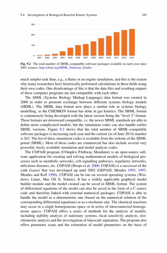
much simpler task than, e.g., a flame or an engine simulation, and this is the reason

why many researchers have historically performed calculations in these fields using

their own codes. One disadvantage of this is that the data files and resulting outputs

of these computer programs are not compatible with each other.

The SBML (Systems Biology Markup Language) data format was created in

2000 in order to promote exchange between different systems biology models

(SBML). The SBML data format now plays a similar role in systems biology

modelling, as the CHEMKIN format has done in gas kinetics. The SBML format

is continuously being developed with the latest version being the “level 3” format.

These formats are downward compatible, i.e. the newer SBML standards are able to

define more complicated models, but the simulation codes can also handle earlier

SBML versions. Figure 9.2 shows that the total number of SBML-compatible

software packages is increasing each year and the current (as of June 2014) number

is 263. The list of these simulation codes is available from the website of the SBML

portal (SBML). Most of these codes are commercial but also include several very

powerful, freely available simulation and model analysis codes.

The COPASI program (COmplex PAthway SImulator) is an open-source soft-

ware application for creating and solving mathematical models of biological pro-

cesses such as metabolic networks, cell-signalling pathways, regulatory networks,

infectious diseases, etc. COPASI (Hoops et al. 2006; COPASI) is a successor of the

code Gepasi that was developed up until 2002 (GEPASI; Mendes 1993, 1997;

Mendes and Kell 1998). COPASI can be run on several operating systems (Win-

dows, Linux, Mac OS X, Solaris). It has a widely applicable graphical model

builder module and the model created can be saved in SBML format. The system

of differential equations of the model can also be saved in the form of a C source

code and therefore linked with external numerical packages. COPASI is able to

handle the model as a deterministic one (based on the numerical solution of the

corresponding differential equations) or as a stochastic one. The chemical reactions

may occur in a single homogeneous space or in series of interconnected homoge-

neous spaces. COPASI offers a series of methods for the analysis of models,

including stability analysis of stationary systems, local sensitivity analysis, stoi-

chiometric analysis and the investigation of timescale separation. The program also

offers parameter scans and the estimation of model parameters on the basis of

Fig. 9.2 The total number of SBML-compatible software packages available in each year since

2001 (source: http://sbml.org/SBML_Software_Guide)

9.4 Investigation of Biological Reaction Kinetic Systems 345

http://sbml.org/SBML_Software_Guide

experimental data, applying any user-defined objective function. The experimental

data may originate from several different sources. The calculated results can be

presented as tables, figures or histograms.

Pre-compiled programs like COPASI facilitate easy use, but many modellers

may wish to check and/or modify the source code of the simulation program. This is

one of the reasons why several Matlab-based programs are distributed for the

simulation and analysis of mathematical models. SBML-SAT is an SBML-based

sensitivity analysis tool (Zi et al. 2008; SBML-SAT) available in Matlab format.

This tool was designed to implement a variety of simulation and analysis techniques

for ODE-based biological models including biophysical models, signalling path-

ways, gene regulation networks and metabolic pathways. SBML-SAT offers not

only simulations but steady-state analysis, robustness analysis, and local and global

sensitivity analyses. The latter includes multiparametric sensitivity analysis, partial

rank correlation coefficient analysis, Sobol’s method and the calculation of the

weighted average of local sensitivities (see Sect. 5.5). Zi et al. also developed an

SBML-based parameter estimation tool in scalar code (SBML-PET) and

parallelised code (SBML-PET-MPI) versions (Zi and Klipp 2006; Zi 2011).

In a rather confusing way, three Matlab toolboxes with similar names are offered

for SBML-based simulations. The “official” SBML-based toolbox, distributed as an

option of Matlab, is called “SimBiology”, whilst the free, academic versions are

called “Systems Biology Toolbox for Matlab” and “SBMLToolbox”. The

“SimBiology” (SimBiology) toolbox provides a graphical environment and pro-

grammatic tools to model, simulate and analyse dynamical systems, focusing on

pharmacokinetic/pharmacodynamic (PK/PD) and systems biology applications. It

provides a block diagram editor for building models. SimBiology uses ODE and

stochastic solvers to simulate the time-dependent profile of drug exposure, drug

efficiency, and enzyme and metabolite levels. It is also possible to investigate

system dynamics and to carry out parameter sweeps, sensitivity analysis and

parameter estimation. Parameter sweep (also called parameter scan) means that the

value of a parameter is changed in stages by sweeping the parameter value through a

user-defined range, whilst the values of all other parameters are kept constant. A new

simulation is carried out for each parameter set and thus allows the systematic

exploration of the effect of changing a single parameter on the simulation results.

The “Systems Biology Toolbox for Matlab” (SBtoolbox; Schmidt and Jirstrand

2006) (the newest version is called “Systems Biology Toolbox 2” or

SBTOOLBOX2) offers systems biologists an open and user extensible environ-

ment. This toolbox also features a wide variety of specialised simulation and

analysis tools, like SBML import and export, deterministic and stochastic simula-

tions, visualisations, steady-state and stability analysis, metabolic control analysis,

stoichiometric analysis, local and global sensitivity analyses, determination of

moiety conservations, bifurcation analysis, and global and local optimisation. The

SBPD is an extension package for the Systems Biology Toolbox 2 (sbtoolbox2),

which allows the combination of models, experiments and measurement data to

projects, automatic generation of C-code simulation models, multiple experiment

and multiple measurement parameter estimation, parameter tuning, analysis of

residuals and model reduction.



http://www.mathworks.com/discovery/pharmacokinetic.html

The other freely distributed program, called “SBMLToolbox” (Keating

et al. 2006; SBMLToolbox), is not intended to be a complete Systems Biology

Toolbox for Matlab, but a platform for getting SBML in and out of Matlab and

serves as a starting point from which users can develop their own functionality.

The PottersWheel (Maiwald and Timmer 2008; PottersWheel) is another Matlab

toolbox that is free for academic research. PottersWheel imports and exports SBML

models, but it is applicable also to any ODE-based modelling. The most useful

feature of this code is that it fits the parameters of a model to several datasets

(multiple experiments) at once whilst determining parameter identifiability and

confidence intervals.

The Systems Biology Workbench (SBW) (SBW; Bergmann and Sauro 2006) is a

software framework that allows heterogeneous applications, written in different

programming languages and running on different platforms to communicate via a

simple network protocol.

9.5 Global Uncertainty Analysis

Several freely downloadable programs can be applied for global uncertainty and

sensitivity analyses (see Sect. 5.5). A Matlab-based toolbox for the application of

HDMR-based global sensitivity analysis is available using the GUI-HDMR pro-

gram (GUI-HDMR). As its name suggests, this is a graphical user interface (GUI)

that allows the application of random sampling HDMR methods (see Sect. 5.5.3)

for the calculation of up to second-order global sensitivity indices and component

functions based on user supplied sets of input/output data. The component functions

are approximated by up to tenth-order orthonormal polynomials. The resulting first-

and second-order sensitivity indices can be used for the interpretation of the

relationships between the inputs and outputs of any numerical model and for the

assessment of the importance and interaction of parameters. The component func-

tions can be visualised and used to explore any nonlinearities in the responses to

parameter changes. The HDMR method can also be used for the generation of a

metamodel that approximates the simulation results as a function of parameters.

The methodology adopted is described in Ziehn and Tomlin (2009).

More recently a similar package called SobolHDMR has been developed by

Kucherenko (2013) and is available on request from the author. In common with the

GUI-HDMR program, it can develop metamodels based on quasi-random inputs but

also includes a metamodelling method based on the use of radial basis functions and

derivative-based sensitivity methods. Explore HD is a third HDMR-based software

package developed by Aerodyne Research based on the methods of the Princeton

Group that were discussed in Sect. 5.5.3 (Aerodyne-Research 2014). This code is

available at a low cost to research groups and offers the ability to handle not only

output from computational simulations but also experimental data. It is also able to

fit up to third-order metamodels (Li et al. 2010).





DAKOTA (DAKOTA) is a GNU GPL-licenced program package developed at

Sandia National Laboratories. DAKOTA is the abbreviation of its longer name

“Design Analysis Kit for Optimization and Terascale Applications”. A calculation

is called “terascale” if 1012 operations per second (teraflop) are carried out on 1012

bytes (terabyte) data. DAKOTA allows the optimisation of models using gradient

and gradient-free methods, and is able to carry out sensitivity and uncertainty

analyses using several methods including the polynomial chaos method described

in Sect. 5.5.2.

SimLab is another comprehensive program package (Simlab 2011) for global

uncertainty analysis. SimLab has been developed at the EC Joint Research Centre

(EC-JRC) in Ispra, Italy. The predecessor of SimLab was a Fortran code called

PREP-SPOP, which was developed from 1985 onwards. This program first (in the

PREP phase) generates parameter sets according to various parameter probability

density functions. The user then has to carry out model simulations using these

parameter sets and the results of the simulations are processed (SPOP) in order to

provide sensitivity measures. Based on the earlier PREP-SPOP code, the develop-

ment of SimLab started in 1999. The first versions of SimLab (up until version 2.2,

2003) are executable Windows application codes. Similarly to PREP-SPOP, the

first step is the generation of parameter sets. As a second step, for simple algebraic

models the program evaluates the simulation results, whilst for more complex

models the user is allowed to generate the simulation results using an external

code. The third step is the processing of the simulation results and the visualisation

of the outcome of uncertainty/sensitivity analyses. SimLab 2.2 is an eye-catching,

easy-to-use code that is excellent for educational purposes. On the other hand, being

a Windows application, it limits the possibilities for an advanced user.

The newer versions of SimLab (from version 3.0, 2004) are program libraries

that can be called from Fortran, Python, C++ or Matlab environments. This

arrangement may not be as intuitive for a beginner as the earlier versions were,

but allows more freedom for advanced users. These new versions include a wider

variety of methods for uncertainty analysis. For example, the parameter sets can be

generated randomly, using Latin hypercube sampling, or according to the FAST,

Morris and Sobol’ methods (see Sect. 5.5). Also, the processing of the simulation

results in order to provide sensitivities includes a series of approaches, including the

FAST, Morris and Sobol’ methods.

SaSAT (Hoare et al. 2008; SaSAT) is a Matlab code for sensitivity and uncer-

tainty analysis. Similarly to the previous codes, SaSAT can generate parameter sets

that correspond to the probability density functions of the parameters. It can

generate random, complete factorial and Latin hypercube samples. Simulations

are then carried out using these samples, and SaSAT calculates the sensitivity

indices or the Pearson, Spearman or partial rank correlation coefficients. The

program is able to approximate the simulation results with a polynomial as a

function of the input parameters (i.e. a metamodel generation). The user is assisted

with a graphical program interface and Excel compatibility, and is able to visualise

input–output relationships using a variety of methods including scatter plots and

response surfaces.




References

ACUCHEM: Chemical kinetics simulation program. http://sourceforge.net/projects/acuchem/

Aerodyne-Research: ExploreHD. http://www.aerodyne.com/products/explorehd (2014)

Bergmann, F.T., Sauro, H.M.: SBW—a modular framework for systems biology. Proceedings of

the 37th conference on winter simulation WSC’06, pp. 1637–1645 (2006)

Brauer, F., Castillo-Chavez, C.: Mathematical Models in Population Biology and Epidemiology.

Springer, New York (2011)

Braun, W., Herron, J.T., Kahaner, D.K.: ACUCHEM—A computer program for modeling com-

plex chemical reaction systems. Int. J. Chem. Kinet. 20, 51–62 (1988)

Cantera: An open-source, object-oriented software suite for combustion. http://sourceforge.net/

projects/cantera/, http://code.google.com/p/cantera/

CHEMKIN/CHEMKIN-PRO Visualization manual, CK-VIS-10101-0810-UG-1. Reaction

Design, San Diego (2010)

COPASI: a COmplex PAthway SImulator. www.copasi.org

Cuoci, A., Frassoldati, A., Faravelli, T., Ranzi, E.: A computational tool for the detailed kinetic

modeling of laminar flames: application to C2H4/CH4 coflow flames. Combust. Flame 160,870–886 (2013a)

Cuoci, A., Frassoldati, A., Faravelli, T., Ranzi, E.: Numerical modeling of laminar flames with

detailed kinetics based on the operator-splitting method. Energy Fuels 27, 7730–7753 (2013b)Daescu, D., Sandu, A., Carmichael, G.R.: Direct and adjoint sensitivity analysis of chemical


37, 5097–5114 (2003)

DAKOTA: Design Analysis Kit for Optimization and Terascale Applications. http://www.cs.

sandia.gov/DAKOTA/


a software environment for solving chemical kinetics. Comp. Chem. Eng. 26, 1567–1579(2002)

Fall, C.P., Marland, E.S., Wagner, J.M., Tyson, J.J.: Computational Cell Biology. Springer,

New York (2005)



Fischer, M., Riedel, U.: Combustion chemistry and parameter estimation. In: Bock, H.G., Carraro,

T., Jager, W., Korkel, S., Rannacher, R., Schloder, J.P. (eds.) Model Based Parameter Estima-

tion. Theory and Applications, vol. 4, pp. 207–226. Springer, Berlin (2013)

FlameMaster. http://www.stanford.edu/group/pitsch/FlameMaster.htm, http://www.itv.rwth-

aachen.de/downloads/flamemaster/ (2014)

FluxViewer: Visualisation tool for element fluxes. http://garfield.chem.elte.hu/Combustion/

fluxviewer.htm

Frenklach, M.: Transforming data into knowledge—process informatics for combustion chemis-

try. Proc. Combust. Inst. 31, 125–140 (2007)

GEPASI: http://www.gepasi.org/

Gokulakrishnan, P., Joklik, R., Viehe, D., Trettel, A., Gonzalez-Juez, E., Klassen, M.: Optimiza-

tion of reduced kinetic models for reactive flow simulations. J. Eng. Gas Turbines Power 136,011503 (2013)

GUI-HDMR: http://www.gui-hdmr.de/

Hoare, A., Regan, D.G., Wilson, D.P.: Sampling and sensitivity analyses tools (SaSAT) for

computational modelling. Theor. Biol. Med. Model. 5, 4 (2008)


Kummer, U.: COPASI—a COmplex PAthway SImulator. Bioinformatics 22, 3067–3074(2006)

Ingber, L., Rosen, B.: Genetic algorithms and very fast simulated re-annealing—a comparison.

Math. Comput. Model. 16, 87–100 (1992)

References 349

http://sourceforge.net/projects/acuchem/

http://www.aerodyne.com/products/explorehd

http://sourceforge.net/projects/cantera/

http://sourceforge.net/projects/cantera/

http://code.google.com/p/cantera/

http://www.copasi.org/

http://www.cs.sandia.gov/DAKOTA/

http://www.cs.sandia.gov/DAKOTA/

http://www.stanford.edu/group/pitsch/FlameMaster.htm

http://www.itv.rwth-aachen.de/downloads/flamemaster/

http://www.itv.rwth-aachen.de/downloads/flamemaster/



http://www.gepasi.org/

http://www.gui-hdmr.de/

Keating, S.M., Bornstein, B.J., Finney, A., Hucka, M.: SBMLToolbox: an SBML toolbox for

MATLAB users. Bioinformatics 22, 1275–1277 (2006)

Kee, R.J., Rupley, F.M., Miller, J.A.: CHEMKIN-II: A FORTRAN chemical kinetics package for

the analysis of gas-phase chemical kinetics. Sandia National Laboratories (1989)

KINAL: program package for the simulation and analysis of reaction mechanisms. http://garfield.

chem.elte.hu/Combustion/kinal.htm

KINALC: CHEMKIN based program for KInetic aNALysis. http://garfield.chem.elte.hu/Combus

tion/kinalc.htm.

Kintecus: http://www.kintecus.com/ (2014)


Kirkpatrick, S.: Optimization by simulated annealing. Science 220, 671–681 (1983)

Kucherenko, S.: SOBOLHDMR: a general-purpose modeling software. In: Polizzi, K.M.,

Kontoravdi, C. (eds.) Synthetic Biology. Methods in Molecular Biology, vol. 1073, pp. 191–

224. Humana, Totowa (2013)

laminarSMOKE web site. http://www.opensmoke.polimi.it/ (2014)

Li, G.Y., Rabitz, H., Yelvington, P.E., Oluwole, O.O., Bacon, F., Kolb, C.E., Schoendorf, J.:

Global sensitivity analysis for systems with independent and/or correlated inputs. J. Phys.

Chem. A 114, 6022–6032 (2010)

LOGE: LOGEsoft v. 1.02. In: Engineering, L.C. (ed.) http://www.loge.se/Products/LOGE_Prod

ucts.html (2014)

Maiwald, T., Timmer, J.: Dynamical modeling and multi-experiment fitting with PottersWheel.

Bioinformatics 24, 2037–2043 (2008)

Maly, T., Petzold, L.R.: Numerical methods and software for sensitivity analysis of differential-

algebraic systems. Appl. Numer. Math. 20, 57–79 (1996)

MECHMOD: Modification of CHEMKIN-format mechanisms. http://garfield.chem.elte.hu/Com

bustion/mechmod.htm

Mendes, P.: GEPASI: a software package for modelling the dynamics, steady states and control of

biochemical and other systems. Comput. Appl. Biosci. 9, 563–571 (1993)

Mendes, P.: Biochemistry by numbers: simulation of biochemical pathways with Gepasi 3. Trends

Biochem. Sci. 22, 361–363 (1997)

Mendes, P., Kell, D.B.: Non-linear optimization of biochemical pathways: applications to meta-

bolic engineering and parameter estimation. Bioinformatics 14, 869–883 (1998)

NAG: Numerical Algorithms Group. www.nag.co.uk (2014)

Nagy, T.: SEM: mechanism reduction based on simulation error minimization. http://garfield.

chem.elte.hu/Combustion/sem.htm (2009)

Nagy, T., Turanyi, T.: Reduction of very large reaction mechanisms using methods based on

simulation error minimization. Combust. Flame 156, 417–428 (2009)

Nagy, A.L., Papp, D., Toth, J.: Reaction Kinetics—A Mathematica package with applications.

Chem. Eng. Sci. 83, 12–23 (2012)

Novak, B., Pataki, Z., Ciliberto, A., Tyson, J.J.: Mathematical model of the cell division cycle of

fission yeast. Chaos 11, 277–286 (2001)

Olm, C., Zsely, I.G., Palvolgyi, R., Varga, T., Nagy, T., Curran, H.J., Turanyi, T.: Comparison of

the performance of several recent hydrogen combustion mechanisms. Combust. Flame 161,2219–2234 (2014)

PottersWheel: Multi-experiment fitting. http://www.potterswheel.de/

PrIMe: Process Informatics Model. http://www.primekinetics.org/

Reaction-Design: Chemkin-Pro. http://www.reactiondesign.com/products/chemkin/chemkin-pro/

(2014)

ReactionDesign: www.reactiondesign.com

Reaction-Engineering-International: CARM (Computer Assisted Reduction Method). http://

energy.reaction-eng.com/modeling_tools/carm.html (2014)


http://garfield.chem.elte.hu/Combustion/kinal.htm

http://garfield.chem.elte.hu/Combustion/kinal.htm



http://www.kintecus.com/


http://www.opensmoke.polimi.it/

http://www.loge.se/Products/LOGE_Products.html

http://www.loge.se/Products/LOGE_Products.html

http://garfield.chem.elte.hu/Combustion/mechmod.htm

http://garfield.chem.elte.hu/Combustion/mechmod.htm

http://www.nag.co.uk/

http://garfield.chem.elte.hu/Combustion/sem.htm

http://garfield.chem.elte.hu/Combustion/sem.htm

http://www.potterswheel.de/

http://www.primekinetics.org/

http://www.reactiondesign.com/products/chemkin/chemkin-pro/

http://www.reactiondesign.com/

http://energy.reaction-eng.com/modeling_tools/carm.html

http://energy.reaction-eng.com/modeling_tools/carm.html


kinetic systems with KPP: Part I – theory and software tools. Atmos. Environ. 37, 5083–5096(2003)

SaSAT: Sampling and sensitivity analyses tools. http://www.nchecr.unsw.edu.au/NCHECRweb.

nsf/page/BioModInfectDis

SBML-SAT: SBML based Sensitivity Analysis Tool. http://g6g-softwaredirectory.com/bio/cross-

omics/pathway-analysis-grns/20258MaxPlanckSBML-SAT.php

SBML: Systems Biology Markup Language. http://sbml.org/

SBMLToolbox: an SBML toolbox for MATLAB users. http://sbml.org/Software/SBMLToolbox

SBtoolbox: Systems Biology Toolbox for MATLAB. http://www.sbtoolbox.org/

sbtoolbox2. http://www.sbtoolbox2.org

SBW: Systems Biology Workbench. http://www.sys-bio.org

Schmidt, H., Jirstrand, M.: Systems biology toolbox for MATLAB: a computational platform for

research in systems biology. Bioinf. Appl. Note 22, 514–515 (2006)

Schuchardt, K., Oluwole, O., Pitz, W., Rahn, L.A., Green, W.H., Leahy, D., Pancerella, C.,

Sjoberg, M., Dec, J.: Development of the RIOT web service and information technologies to

enable mechanism reduction for HCCI simulations. J. Phys. Conf. Ser. 16, 107–112 (2005)

Schuchardt, K., Pancerella, C., Rahn, L.A., Didier, B., Kodeboyina, D., Leahy, D., Myers, J.D.,

Oluwole, O.O., Pitz, W., Ruscic, B., Song, J., von Laszewski, G., Yang, C.: Portal-based

knowledge environment for collaborative science. Concurr. Comput. Pract. Exp. 19, 1703–1716 (2007)

Sedaghat, A.R., Sherman, A., Quon, M.J.: A mathematical model of metabolic insulin signaling

pathways. Am. J. Physiol. Endocrinol. Metab. 283, E1084–E1101 (2002)

SimBiology: Model, simulate, and analyze biological systems. http://www.mathworks.com/prod

ucts/simbiology/

Simlab: Software package for uncertainty and sensitivity analysis. Joint Research Centre of the

European Commission. http://simlab.jrc.ec.europa.eu (2011)

SUNDIALS: SUite of Nonlinear and DIfferential/ALgebraic equation Solvers. http://computation.

llnl.gov/casc/sundials/

Sung, C.J., Law, C.K., Chen, J.Y.: Augmented reduced mechanisms for NO emission in methane

oxidation. Combust. Flame 125, 906–919 (2001)

Tenua: the kinetics simulator for Java. http://bililite.com/tenua/

Turanyi, T.: KINAL - A program package for kinetic-analysis of reaction-mechanisms. Comput.

Chem. 14, 253–254 (1990)

Vol’pert, A.I.: Дифференциальные уравнения на графах. Мат. Сборник 88, 578–588 (1972)

WINPP/XPP: http://www.math.pitt.edu/~bard/classes/wppdoc/readme.htm

Wolfram, S.: Mathematica Language. http://www.wolfram.com/mathematica/. Accessed April

2014

Zi, Z.: SBML-PET-MPI: a parallel parameter estimation tool for Systems Biology Markup

Language based models. Bioinformatics 27, 1028–1029 (2011)

Zi, Z., Klipp, E.: SBML-PET: a Systems Biology Markup Language-based parameter estimation

tool. Bioinformatics 22, 2704–2705 (2006)

Zi, Z., Zheng, Y., Rundell, A.E., Klipp, E.: SBML-SAT: a systems biology markup language

(SBML) based sensitivity analysis tool. BMC Bioinform. 9, 342 (2008)

Ziehn, T., Tomlin, A.S.: GUI-HDMR—A software tool for global sensitivity analysis of complex

models. Environ. Model. Software 24, 775–785 (2009)

References 351

http://www.nchecr.unsw.edu.au/NCHECRweb.nsf/page/BioModInfectDis

http://www.nchecr.unsw.edu.au/NCHECRweb.nsf/page/BioModInfectDis

http://g6g-softwaredirectory.com/bio/cross-omics/pathway-analysis-grns/20258MaxPlanckSBML-SAT.php

http://g6g-softwaredirectory.com/bio/cross-omics/pathway-analysis-grns/20258MaxPlanckSBML-SAT.php

http://sbml.org/

http://sbml.org/Software/SBMLToolbox

http://www.sbtoolbox.org/

http://www.sbtoolbox2.org/

http://www.sys-bio.org/

http://www.mathworks.com/products/simbiology/

http://www.mathworks.com/products/simbiology/

http://simlab.jrc.ec.europa.eu/

http://computation.llnl.gov/casc/sundials/

http://computation.llnl.gov/casc/sundials/

http://bililite.com/tenua/

http://www.math.pitt.edu/~bard/classes/wppdoc/readme.htm

http://www.wolfram.com/mathematica/

Chapter 10

Summary and Concluding Remarks

Almost every chemical process includes many reaction steps. This means that the

reactants will first produce intermediates, which will then be involved in further

reactions leading to the final products. Frequently, the final products of the chemical

process appear only after several hundreds or thousands of different reaction steps.

The products may include those that are desired (e.g. yields of valuable chemicals

or energy) and those that are unwanted, such as pollutants. If the stoichiometric

equations and the rates of each reaction step are known, then the chemical process

can in principle be controlled. In industrial applications this means that the com-

position of the reacting mixture and the conditions of the reaction process can be

selected so that the process operates as efficiently as possible and has low environ-

mental impact. Simulations of detailed reaction mechanisms can therefore be

extremely useful within the design phase of new equipment or for the development

and control of existing equipment. If a model is accurate and robust, and can be

simulated efficiently, then it can be used in place of expensive experiments for

process design. Within the book we have tried to address methods that can be used

to assess and improve the robustness of kinetic mechanisms, as well as to reduce

their impact on the simulation time of models of coupled chemical and physical

processes. The aim of all of these methods is to improve the utility of kinetic

mechanisms for a range of applications in the real world.

Detailed reaction mechanisms are also used for the simulation of atmospheric

chemical processes. These days a numerical weather prediction model can predict

air temperature, solar radiation, wind speed and direction, and atmospheric stability

with reasonably good accuracy and spatial resolution several days in advance. This

means that by coupling a detailed atmospheric reaction mechanism to the meteo-

rological forecast, and including appropriate emissions data, predictions of air

quality can also be achieved in advance. This information could be used, for

example, to impose a smog/health alert well before the onset of the actual environ-

mental problem. In certain cases, such forecasts have also been used to inform

short-term emission control strategies, such as reducing traffic volume in major

cities (e.g. the banning of cars with even number plates in Paris on 17 March 2014).



353

Such models can also be used for the strategic assessment of air quality by testing

emission reduction plans prior to implementation using air quality simulation

models. In atmospheric applications, models are perhaps even more critical than

within industrial design, since it is often difficult to propose and to evaluate

“experiments” within the open atmosphere. Nevertheless, the models need to be

grounded in reality, and hence investigations of their robustness and methods for

their constant improvement are essential.

Detailed reaction mechanisms are also frequently used for the simulation of

combustion processes. Chemical energy is converted to electrical energy within

power stations and to mechanical energy within engines. Based on accurate and

robust descriptions of the relevant combustion processes, the efficiency of furnaces

and engines can be improved. Designs can also be sought which lead to a simul-

taneous decrease in environmental impacts. The interaction between complex

chemical and physical processes such as turbulent flows makes this an extremely

challenging problem. However, the use of models can assist in design optimisation,

with the aim that the same power should be obtained with decreased emissions of

harmful pollutants. Combustion is one area where the use of reduced chemical

models has seen a very wide range of applications as discussed in the preceding

chapters.

A relatively new but rapidly developing area for the application of detailed

reaction mechanisms is in the modelling of biochemical processes. Nowadays,

there are several molecular biological systems for which the participating species

are known, and also the stoichiometry and rate coefficients of the chemical reac-

tions can at least be suggested, if not known with a high degree of certainty. These

include metabolism networks, signal transduction and cell cycle regulation. Kinetic

mechanisms for all these systems are beginning to emerge. Using more detailed

chemical knowledge, the concentration–time profiles of the biomolecules can be

calculated, allowing a much deeper insight to the functioning of the biological

systems on a molecular level. This can facilitate new paradigms for the develop-

ment of medical drugs.

One of the signs of development within the field of reaction kinetics is that more

and more processes are being described by increasingly detailed reaction mecha-

nisms. The consequence is that the available mechanisms are getting larger, and

contain significantly more species and reaction steps. It is critically important that

simulations based on these detailed mechanisms are able to reproduce wider sets of

experimental data with good accuracy. This becomes challenging, since many of

the parameters within large and detailed mechanisms have not been studied indi-

vidually but, for example, are quantified based on structural similarities with better

known species/reaction steps. The use of sensitivity analysis therefore becomes

invaluable, since it can help to identify where the focus on mechanism improve-

ment should be placed. Whilst the discussion in this text centres on model simula-

tions, we should not underestimate the importance of experimental data in its

contributions towards model improvement and evaluation. Experiments provide

the constraints required to reduce the uncertainty within the key parameters of

kinetics mechanisms. By expanding the experimental datasets available to model

354 10 Summary and Concluding Remarks

developers, it is expected, therefore, that the predictivity of the models will also

improve. By better constraining the models, they should provide good results even

at conditions that have not yet been studied experimentally or that cannot be

investigated for technical reasons.

Another sign of development is that a growing number of thermokinetic param-

eters are accompanied by estimations of their accuracy. In the best cases, these

uncertainty estimates are based not on the error analysis of a single experiment but

reflect the comparison of several independent experimental or theoretical studies

and therefore incorporate systematic errors of the various methods. In the past, such

evaluations were performed by human experts, but as the dataset grows, perhaps a

new paradigm for this process is required. Data collaboration approaches have been

suggested which could place this task in the hands of wide communities (and

computer software), rather than small groups of experts.

Where mechanisms become suitably robust, new approaches to gaining chem-

ical knowledge become feasible based on the analysis of simulation results. For

example, the concentrations of species could be estimated that are not accessible

experimentally for the conditions of interest. Kinetic analyses can then be

performed providing information on the most important reaction pathways, on

interactions between the various subprocesses in a system and on the kinetic

parameters that are key to obtaining good simulation results.

Most chemical kinetic systems of practical importance are likely to be spatially

inhomogeneous, i.e. the concentrations and the temperatures will be different at

different locations. Photochemical air pollution, flame and engine combustion

models are good examples of spatially inhomogeneous systems, where chemical

processes interact with often quite complex physical processes such as turbulent

flows. In general, the validation of chemical mechanisms is achieved by attempting

to simulate experimental setups which simplify these complex flow processes, thus

allowing focus on the chemical changes. Examples of such experiments would

include well-mixed smog chamber studies for atmospheric chemical mechanisms

or, flat or axially symmetric flames in combustion. In these cases the concentrations

and temperature are either homogeneous or change along only one or two spatial

coordinates. The corresponding models are called spatially 0D, 1D or 2D, respec-

tively, and can often be simulated using a detailed reaction mechanism. Detailed

chemistry can therefore be evaluated by comparing models with target quantities

from such types of experiments incorporating methods for uncertainty and sensi-

tivity analysis as described within Chap. 5. 3D models of practically relevant flows

usually have to use reduced reaction mechanisms in order to lower the computa-

tional cost. Where possible such a reduced model should be based on a well-

validated detailed model and developed using formal reduction procedures which

attempt to minimise simulation errors as discussed in Chap. 7. Reduced mecha-

nisms also have application in situations where the model must provide an answer

within a short time, e.g. to make them applicable in real-time simulations of

environmental catastrophes involving chemical processes such as pollution

hazards.

10 Summary and Concluding Remarks 355

http://dx.doi.org/10.1007/978-3-662-44562-4_5

http://dx.doi.org/10.1007/978-3-662-44562-4_7

The purpose of this book was to describe a range of analysis tools that may assist

in the development of chemical mechanisms of use within practical simulation

codes for real-world problems. At the beginning of the book, basic information on

chemical kinetic modelling was summarised. Chapter 2 could therefore be used

within introductory classes on reaction kinetics, environmental science or engi-

neering. Although most detailed mechanisms used nowadays have been compiled

by human effort, this approach is not feasible when mechanisms consist of several

thousand reaction steps. Therefore, the automatic generation of reaction mecha-

nisms is becoming increasingly important and was described in Chap. 3. Such

methods build on the increasing ability of kinetics communities to describe and

quantify chemical pathways for important classes of reactions and have seen

applications in the fields of atmospheric chemistry, combustion and more recently

systems biology. Consistent ways to interpret these reaction pathways were intro-

duced in Chap. 4.

Despite the best efforts of kinetics researchers, uncertainties still exist in most

chemical mechanisms either in their parameterisations or within the structure of the

model. The analysis of the robustness of models is therefore important and a

number of sophisticated methods have been developed for the analysis of detailed

reaction mechanisms. One family of such methods investigates the uncertainty of

the simulation results due to the uncertainty in the parameters, and initial and

boundary conditions (Chap. 5). These methods provide the variance or even the

joint probability density function of the model results. When coupled with sensi-

tivity analysis, they can be used to trace the origin of the uncertainty, i.e. to show

which parameter uncertainties are mainly responsible for the uncertainty in the

simulation results. This highlights where future efforts for model improvement

should be placed in order to improve the robustness of models and therefore their

ability to be “predictive”.

Timescales are important features of dynamical models. Whilst historically we

may be used to identifying individual timescales with individual species within a

mechanism, we demonstrated in Chap. 6 that within a nonlinear kinetic model,

there is usually not a one-to-one relationship between them. Nevertheless, we

showed that the relationship between species and timescales, and the dynamic

changes in timescales during a model simulation, can be explored using perturba-

tion methods. Timescales are related to the stiffness of dynamical models, which is

an important feature for the selection of appropriate numerical simulation methods.

However, the wide range of timescales and the timescale separation can be

exploited within the context of model reduction, and therefore, there are important

links between Chaps. 6 and 7 in this regard.

As knowledge of chemical, physical and biological processes improves, so does

the ability to describe kinetic systems with increasing levels of detail. Over time

therefore, reaction mechanisms have tended to become larger, both in terms of

numbers of species and elementary reaction steps. However, when a reaction

mechanism is used within a simulation code, a smaller mechanism is usually

more desirable from a computational point of view. The aim of mechanism

reduction methods (Chap. 7) is to find the smallest reaction mechanism

356 10 Summary and Concluding Remarks

http://dx.doi.org/10.1007/978-3-662-44562-4_2

http://dx.doi.org/10.1007/978-3-662-44562-4_3

http://dx.doi.org/10.1007/978-3-662-44562-4_4

http://dx.doi.org/10.1007/978-3-662-44562-4_5

http://dx.doi.org/10.1007/978-3-662-44562-4_6

http://dx.doi.org/10.1007/978-3-662-44562-4_6

http://dx.doi.org/10.1007/978-3-662-44562-4_7

http://dx.doi.org/10.1007/978-3-662-44562-4_7

(or mathematical model) that is able to predict important features or the concen-

trations of important species to within good agreement with the full model for the

reaction conditions of interest. Reduction of reaction mechanisms can be based on

the search for a subset or skeletal mechanism (by eliminating redundant species and

reactions), the lumping of species and reactions, or a timescale analysis of the

model. The point of all of these methods is that the reduced model need not

necessarily resolve all scales of the original model but need only predict important

observables. This can apply in the context of timescales, where those much shorter

or much longer than the characteristic timescale can be eliminated, or in the context

of species concentrations, where intermediates may not be required, or a lumped

quantity may be sufficient rather than resolving large numbers of individual con-

centrations (e.g. for VOCs). Over time increasingly sophisticated methods for

model reduction have been elaborated beginning with the classic kinetic simplifi-

cation principles described in Sect. 2.3, up to numerical theories based on, e.g.,

CSP, or invariant manifold theories.

The final discussion of the book focused on a perhaps surprising feature of

kinetic systems, namely, the similarity of their local sensitivity functions. It was

shown that for certain conditions, there can be strict relations among these func-

tions, such as having similar shapes. The origin of these relations was discussed in

Chap. 8, and their consequence on the uniqueness of models and on the estimation

of their parameters from experimental data was explored. These important features

of the local sensitivity functions have been detected in combustion and systems

biology models.

The methods and algorithms described in this book are sometimes very compli-

cated. Fortunately, for almost all methods, computer codes facilitating their appli-

cation can be downloaded from the Internet. In Chap. 9 many such codes were

introduced with the discussion organised according to the following topics: simu-

lation of isothermal homogeneous chemical kinetic systems, gas kinetics, analysis

of reaction mechanisms, uncertainty analysis and investigation of biological reac-

tion systems.

In spite of all efforts, errors may remain within the text of this book. The authors

would highly appreciate receiving notifications by e-mail ([email protected] [email protected]) about any errors discovered by readers. A list of

errors and other news concerning the book will be published on the following

Web site:

http://garfield.chem.elte.hu/Turanyi/KineticReactionMechanisms.html

Acknowledgements The authors of the book are indebted to several people who made sugges-

tions to earlier versions of the manuscript. We acknowledge the valuable comments and sugges-

tions of Drs. Janos Toth, Judit Zador, Tibor Nagy, Istvan Gy. Zsely, Anna Lovrics and Mr. Carsten

Olm. We also thank Carsten Olm, Istvan Gy. Zsely and Tilo Ziehn for preparing several figures.

Tamas Turanyi acknowledges the support of Hungarian Science Foundation OTKA K84054.

10 Summary and Concluding Remarks 357


http://dx.doi.org/10.1007/978-3-662-44562-4_8

http://dx.doi.org/10.1007/978-3-662-44562-4_9

http://garfield.chem.elte.hu/Turanyi/KineticReactionMechanisms.html

Index

AActivation temperature, 18

Active mode, 161–163

Active thermochemical table (ATcT), 113

ACUCHEM program, 338

Adaptive chemistry, 196, 201, 256, 287,

288, 290

Adaptive reduced mechanism, 287, 288

Analysis of variances (ANOVA)

decomposition, 93, 95

Analytical solution, 14, 28, 314

ANN. See Artificial neural network (ANN)

Approximate slow invariant manifold (ASIM),

258

Arrhenius equation, 18, 106, 314

Arrhenius plot, 18

Artificial neural network (ANN), 282–286

ASIM. See Approximate slow invariant

manifold (ASIM)

ATcT. See Active thermochemical table

(ATcT)

Automatic differentiation, 69, 289

Automatic differentiation in Fortran

(ADIFOR), 70, 91

Autonomous system of ODEs, 12, 317

BBackward reaction, 29

Bath gas, 9, 22

Bimolecular reaction, 9, 24

Binary search tree (BST), 265

Bodenstein-principle. See Quasi-steady-stateapproximation (QSSA)

Branching ratio, 33, 106

Brute force method, 66–69, 126

BST. See Binary search tree (BST)

CCantera program, 341

Cell cycle, 2, 70, 168, 325, 330, 332, 334

CEM. See Constrained equilibrium manifold

(CEM)

Channel ratio, 33

Characteristic timescale, 172, 244, 272, 357

CHEMATA code, 44

Chemical explosive mode analysis, 157

Chemical Kinetics Simulator (CKS) program,

338

Chemical lumping, 211

CHEMKIN program package, 339, 342

Circadian clock models, 12, 70, 209, 244

Cluster analysis, 290, 328

CM. See Connectivity method (CM)

Collision efficiency, 22

Common representative intermediates (CRI)

mechanism, 216

Complementary set of species, 189

Complex-forming bimolecular reaction, 9, 24

Computational singular perturbation (CSP),

160, 186, 202, 239, 242, 253, 287, 343

importance index, 243

participation index, 243

pointer, 244

Computer Assisted Reduction Method

(CARM) program package, 344

Connectivity method (CM), 187, 201

Conserved moiety, 32, 346

Conserved property, 32, 54


T. Turanyi, A.S. Tomlin, Analysis of Kinetic Reaction Mechanisms,DOI 10.1007/978-3-662-44562-4

359

Consistent mechanism, 189

Constrained equilibrium manifold (CEM), 255,

269

Constrained species lumping, 221

Continuous species, 227

COPASI program, 250, 345

CSP. See Computational singular perturbation

(CSP)

DDAC. See Dynamic adaptive chemistry (DAC)

DAKOTA program package, 348

Data collaboration, 48, 342

Decoupled direct method (DDM), 68, 128

Direct method, 68

Directed relation graph (DRG) method, 193,

196, 201

DRG-aided sensitivity analysis (DRGASA),

197, 201

DRGEP-aided sensitivity analysis (DRGEP-

ASA), 199, 201

DRG with error propagation (DRGEP), 198

Dynamic adaptive chemistry (DAC), 288

Dynamical dimension, 166, 250, 275, 313, 326

EE-CELL code, 45

ELDM. See Empirical low-dimensional

manifold (ELDM)

Ellipsoid of accuracy (EOA), 264, 266, 285

Empirical low-dimensional manifold (ELDM),

274

EOA. See Ellipsoid of accuracy (EOA)

Equivalence ratio, 115

ESAC. See Exact-steady-state adaptivechemistry (ESAC)

Exact-steady-state adaptive chemistry (ESAC),

291

EXGAS code, 43, 212

Explicit methods for the solution of ODEs,

173, 241

Extended Arrhenius equation, 19

External species, 16

FFall-off region, 21

Family method, 216, 230

FAST. See Fourier amplitude sensitivity test

(FAST)

Fast equilibrium approximation. See Pre-equilibrium approximation

Fast equivalent operational model (FEOM),

281

Fast variable, 151, 176, 226, 232, 268

FEOM. See Fast equivalent operational model

(FEOM)

FGM. See Flamelet generated manifolds

(FGM)

First-order sensitivity index, 86, 90, 98,

100, 202

Flamelet generated manifolds (FGM), 270

FlameMaster program, 341

Flame prolongated ILDM (FPI), 270

Flow-controlled chemistry tabulation (FCCT)

method, 262

Flux balance analysis (FBA), 58

FluxViewer program, 55, 343

Forward reaction, 29

Fourier amplitude sensitivity test (FAST), 88,

96, 129, 348

Functional principal component analysis

(fPCA), 190

Functional sensitivity analysis, 68

GGA. See Genetic algorithm (GA)

Gaussian error propagation rule, 74

Gaussian process emulator methods, 92

Genetic algorithm (GA), 206, 209, 239, 288

Genetic regulatory network (GRN) model, 230

GeneWays code, 44

Gepasi program, 345

Global error, 205, 235, 266–268

Global sensitivity analysis, 63, 75, 79, 100,

105, 119–125, 207, 346, 347

Global similarity, 315, 317, 322, 324, 326, 328,

330

Global uncertainty analysis, 75, 116, 122, 131,

340, 347

Greedy approach, 204, 205, 231, 256

Green function, 67, 237, 273, 322

GUI-HDMR program, 347

HHalf-life, 146

HDMR. See High-dimensional model

representation (HDMR)

Heuristics-aided quantum chemistry (HAQC)

methodology, 44

360 Index

High-dimensional model representation

(HDMR), 91, 95–100, 119–122, 126,

130, 281, 347

Horner representation, 279

IILDM. See Intrinsic low-dimensional manifold

(ILDM) algorithm

Implicit methods for the solution of ODEs,

173, 241

Important feature, 185, 232, 237

Important species, 39, 185–189, 193, 201, 207,

221, 232, 237, 290, 334, 357

Impulse parametric sensitivity analysis (iPSA),

68

Induction period, 237, 239

Information-theoretic sensitivity analysis, 88

Initial concentration sensitivity coefficient. SeeGreen function

In situ adaptive tabulation (ISAT), 263, 269,

285, 286

Internal species, 16

Intrinsic low-dimensional manifold (ILDM)

algorithm, 164, 226, 246, 247, 249–253,

257, 268, 274, 343

Invariant constrained equilibrium edge

preimage curve (ICE-PIC) method, 257,

267–269

Irreversible reaction step, 26

ISAT. See In situ adaptive tabulation (ISAT)

KKINALC program, 188, 342

KINAL program package, 338

Kinetic reaction mechanism, 8

Kinetic simplification principles, 28, 314

Kinetic system of ODEs, 11, 14, 17

Kintecus program, 340

KPP program, 70, 174, 338

Kyoto encyclopaedia of genes and genomes

(KEGG) database, 44

LLaminarSMOKE program, 341

Latin hypercube sampling, 80, 91, 115, 129, 348

Law of mass action, 10, 14, 16, 17, 46

Level of importance (LOI) index, 238, 256

Lifetime, 146–151, 156, 158, 160, 171, 222,

236–238, 257, 260, 343

Lindemann approach, 21–23, 25, 314

Linear species lumping, 218

Living species, 189

Local error, 195, 206, 235, 238, 264–268, 343

Local similarity, 315–318, 321, 323, 329

Local uncertainty analysis, 74, 111–115, 118,

128, 130, 343

LOGEsoft code, 342

Log p formalism, 25

LOI. See Level of importance (LOI) index

Lotka–Volterra model, 2Lumped reaction mechanism, 218

Lumping, 17, 33, 42, 210–231

MMAMOX code, 42

Mass action kinetics, 10, 34, 338

Master chemical mechanism (MCM), 40, 43,

44, 216, 222, 240

Mechacut program, 344

MECHMOD program, 343

MEPT. See Minimal entropy production

trajectory (MEPT) method

Metabolism network, 2, 354

Method of invariant grid (MIG), 258

Method of invariant manifold (MIM), 258

Minimal entropy production trajectory (MEPT)

method, 259

Mode, 158, 166

Modified Arrhenius equation, 19, 106, 314

Molecularity, 9

Molecular signal transfer, 2

Moment-independent global sensitivity

analysis methods, 100

Monte Carlo uncertainty analysis, 79, 82, 86,

109, 115, 118, 129, 341

Morris method, 77, 97, 122, 129

Multichannel reactions, 33, 106

NNASA polynomials, 26, 47, 119, 341

Necessary species, 185, 187–191, 201

Negative cross effect, 17

Network of computed reaction enthalpies to

atom-based thermochemistry (NEAT),

114

NF-κB signalling pathway, 127, 231, 242

Nominal parameter set, 75, 117

Nonautonomous system of ODEs, 12

Nonlinear species lumping, 218, 224–229

Index 361

Nonreactive collisions, 9

NORA. See NO relaxation approach (NORA)

method

NO relaxation approach (NORA) method, 262

Normalised sensitivity coefficient, 65

OOANN. See Optimal artificial neural network

(OANN)

Odd oxygen species, 216

On-the-fly mechanism reduction, 198, 242,

288, 290

Operator splitting, 175, 263, 265, 268, 272,

290–291

Optimal artificial neural network (OANN), 285

Orthonormal polynomials, 91, 97, 251, 277, 347

Oscillating reactions, 13, 15, 32, 70, 146, 185, 273

Overall order of a reaction, 7

Overall reaction equation, 5, 114

Overall sensitivity, 71, 187

PPairwise mixing stirred reactor (PMSR), 266,

289, 290

Partial equilibrium approximation. See Pre-equilibrium approximation

Path flux analysis (PFA) method, 188, 200, 290

PBPK. See Physiologically based

pharmacokinetic (PBPK) model

PCAF method. See Principal component

analysis of matrix F (PCAF)PCAS method. See Principal component

analysis of matrix S (PCAS)

PEA. See Pre-equilibrium approximation

(PEA)

Phase response curve (PRC), 209

Phase space, 13, 158, 163–166, 168

Physiologically based pharmacokinetic

(PBPK) model, 229, 231

PMSR. See Pairwise mixing stirred reactor

(PMSR)

POD. See Proper orthogonal decomposition

(POD)

Pool chemical approximation, 16, 17, 28, 173

Pool component approximation. See Poolchemical approximation

PottersWheel toolbox for MATLAB, 347

PRC. See Phase response curve (PRC)Pre-equilibrium approximation (PEA), 29, 227,

244, 291, 314

PREP-SPOP program package, 348

PrIMe collaboration, 47, 340, 342

Principal component analysis of matrix F(PCAF), 190–192, 343

Principal component analysis of matrix S(PCAS), 72, 190–192, 343

Principal component analysis (PCA) of the

composition space, 247, 274

Production rate, 7, 12, 14, 30, 151, 191, 254, 314

Proper orthogonal decomposition (POD), 274,

286, 290

Proper species lumping, 218, 231

Pseudo-first-order approximation, 29

QQuasi-steady-state approximation (QSSA),

30–32, 42, 74, 152, 161, 174, 199, 211,

217, 227, 231–242, 244, 249, 268, 291,

338, 343

RRadial design method, 79, 130

Range identification and optimization tool

(RIOT) code, 289

Rate coefficient, 7, 14, 18, 191, 212, 314

Rate constant, 7

Rate-controlled constrained equilibriummethod

(RCCE), 253, 257, 267–269, 286

Rate determining step, 30, 33, 186, 198, 240

Rate-of-production analysis, 189–192, 343

RCARM code, 43

RCCE. See Rate-controlled constrained

equilibrium method (RCCE)

Reachable species, 189

REACTION\ANALYSIS code, 43

Reaction channel, 33

Reaction–diffusion manifold (REDIM)

method, 171, 252

Reaction invariant, 32

ReactionKinetics program, 344

Reaction mechanism, 8

Reaction order with respect to species, 7

Reaction pathway analysis, 53

Reaction rate, 7

Reaction step, 8

REDIM. See Reaction–diffusion manifold

(REDIM) method

Redundant species, 185–189, 196, 197, 204,

242, 343

Repro-modelling, 260, 272

Response surface methods (RSMs), 90–100

Reversible reaction step, 26

362 Index

rkmGen program, 344

RMG code, 42

SSAB. See Sensitivity analysis based (SAB)

method

SaSAT program, 348

SBML-PET-MPI program, 346

SBML-PET program, 346

SBML-SAT program, 346

SBML toolbox for MATLAB, 346

Scaling law, 315, 318

Screening methods, 76, 97, 129

Second-order sensitivity index, 86, 87, 100

Self-organising map (SOM), 284

SEM-CM. See Simulation error minimization

connectivity method (SEM-CM)

Seminormalised sensitivity coefficient, 65

SEM program package, 344

Sensitivity analysis, 61–70, 86–100

Sensitivity analysis based (SAB) method, 276

Sensitivity coefficient, 30, 64–69, 75, 93, 276

Sensitivity index, 86, 100

Sensitivity matrix, 65, 191, 318

SIM. See Slow invariant manifold (SIM)

SimBiology toolbox for MATLAB, 346

SimLab program package, 348

Simulated annealing optimisation, 209

Simulation error, 183, 188, 201, 344

Simulation error minimization connectivity

method (SEM-CM), 188, 205, 344

Skeletal model reduction, 184

Slow invariant manifold (SIM), 161, 242, 251,

257, 259, 268, 274

Slow manifold, 163, 164, 170, 234, 239, 258,

319, 343

Slow variable, 151, 164, 232, 242

SOM. See Self-organising map (SOM)

Stiffness index, 172

Stiffness ratio, 172

Stiff system of differential equations, 12, 32,

69, 145, 172, 222, 232, 233, 291, 338

Stochastic kinetic modelling, 14, 63, 338, 346

Stoichiometric coefficient, 6, 8, 15, 17, 54

Stoichiometric equation, 5

Stoichiometric matrix, 8, 10, 33

SUite of Nonlinear and DIfferential/ALgebraic

equation Solvers (SUNDIALS) program

package, 338

Symbolic solution, 14, 70, 174

Systems biology markup language (SBML)

data format, 345, 347

Systems biology toolbox for MATLAB, 346

Systems Biology Workbench (SBW) program,

347

TTenua program, 338

THERGAS code, 47

THERM code, 47

Third body, 9, 20, 22, 26

Timescale, 17, 31, 34, 45, 145, 152–175, 217,

222–224, 226, 227, 230-232, 242–245,

251, 257, 272, 274

Titan, the moon of Saturn, 105

Total sensitivity index, 87

Trajectory, 13, 71, 151, 156, 161–164, 176,

187, 201, 238, 249, 257, 265, 268, 316

Troe parameterisation, 23

UUncertainty analysis, 61

Uncertainty parameter f, 92, 102Unimolecular reaction, 9, 21, 24

VVariable volume tabulated homogeneous

chemistry (VVTHC) approach, 262

Index 363

analysis of kinetic reaction mechanisms

Documents