A HISTORY-FRIENDLY MODEL OF THE CO-EVOLUTION OF

THE COMPUTER AND SEMICONDUCTORS INDUSTRIES:

CAPABILITIES AND TECHNICAL CHANGE

AS DETERMINANTS OF THE VERTICAL SCOPE OF FIRMS

IN RELATED INDUSTRIES

Franco Malerba* Richard Nelson** Luigi Orsenigo*** and Sidney Winter****

* CESPRI, Bocconi University, Milan, Italy

** Columbia University, New York *** University of Brescia and CESPRI, Bocconi University, Milan, Italy

**** Wharton School, University of Pennsylvania, Philadelphia

FIRST PRELIMINARY DRAFT. PLEASE DO NOT QUOTE

January 2006.

Anna De Paoli, Andea Pozzi and Davide Sgobba provided an invaluable contribution to the development of the model. Support from the Italian National Research Council (CNR) and from Bocconi University (Basic Research Program) is gratefully acknowledged.

1

ABSTRACT

A HISTORY-FRIENDLY MODEL OF THE CO-EVOLUTION OF THE COMPUTER AND SEMICONDUCTORS INDUSTRIES: CAPABILITIES AND TECHNICAL CHANGE AS DETERMINANTS OF THE VERTICAL SCOPE OF FIRMS IN RELATED INDUSTRIES

by Franco Malerba, Richard Nelson, Luigi Orsenigo and Sidney Winter In this paper we present a history-friendly model of the evolution of the computer and semiconductor industries, focusing on the determinants of the changing vertical scope of computer firms. The model is “history friendly”, in that it attempts at replicating some basic, stylized qualitative features of the evolution of the two industries on the basis of the causal mechanisms and processes which we believe can explain their history. The specific question addressed in the model is set in the context of dynamic and uncertain technological and market environments, characterized by periods of technological revolutions punctuating periods of relative technological stability and smooth technical progress. The model illustrates how the patterns of vertical integration and specialization in the computer industry change as a function of the evolving levels and distribution of firms’ capabilities over time and how they depend on the co-evolution of the upstream and downstream sectors. Specific conditions in each of these markets – i.e. the size of the external market, the magnitude of the technological discontinuities, the lock-in effects in demand – exert critical effects and feedbacks on market structure and on the vertical scope of firms as time goes by.

2

1. Introduction In this paper we present a history-friendly model of the evolution of the computer and semiconductor industries, focusing on the determinants of the changing vertical scope of computer firms. The model is “history friendly”, in that it attempts at replicating some basic, stylized qualitative features of the evolution of the two industries on the basis of the causal mechanisms and processes which we believe can explain their history. The specific question addressed in the model - the determinants of vertical integration and specialization – is set in the context of dynamic and uncertain technological and market environments, characterized by periods of technological revolutions punctuating periods of relative technological stability and smooth technical progress. The proposed interpretation of the dynamics of vertical integration and specialization is centered on firms’ capabilities, technological change and on the co-evolution of the upstream and downstream industries.

The paper is organized as follows. First, we present a brief discussion of the methodology

underlying history-friendly models. Second, we discuss the theoretical background inspiring the interpretation of the history and the model. Section 4 provides a brief description of the historical patterns of vertical integration and specialization in the computer and semiconductor industries. Next, in Section 5, the formal model is presented. In Section 6, we report the results of the history-friendly simulation as well as some counterfactual exercises. Section 7 concludes the paper. 2. History-friendly models

“History-friendly” models (HFMs) are formal models which aim to capture - in stylized form- qualitative theories about mechanisms and factors affecting industry evolution, technological advance and institutional change put forth by empirical research in industrial organization, in business organization and strategy, and in the histories of industries. A discussion of the purposes and limitations of this style of analysis has been provided in earlier papers, which focused on the evolution of – respectively – the computer and pharmaceutical industries (Malerba et al., 1999 and 2001; Malerba and Orsenigo, 2002). Here, suffice it to recall that HFMs are inspired by the recognition that there is a tension between detailed-rich, empirical and historical accounts of specific phenomena and “general theories”, almost always formalised in mathematical models. HFMS have been developed as an attempt at building a closer and more rigorous dialogue with historical and empirical accounts concerning the evolution of specific industries. In particular, HFM try to build a bridge between different phases of the process of economic analysis, in particular between empirical analysis, appreciative theorising, formal modelling and the attempt of constructing general theories.

Moreover, HFMs force the analyst to impose stronger empirical discipline to earlier evolutionary models. The latter proved very successful – in our view – in broadly exploring the logic of evolutionary economic processes, in demonstrating the feasibility of the theoretical and methodological approach and in reproducing some general “stylized facts” concerning industrial evolution. For example, the model developed by Nelson e Winter (1982) aimed mainly to demonstrate that - in an evolutionary context - high innovation rates generate a very concentrated industrial structure. Likewise, Dosi et al. (1995) showed that, according to certain hypotheses about the nature of firms' learning processes and the kind of market selection, a model - also a very simple one– can generate industrial structures with very different characteristic pertaining to rates of entry and exit, concentration, patterns of stability or turbulence, distribution of firms' size, etc.

3

However, this very success feeds a greater ambition. Thus, one should start trying to identify more precisely the crucial, fundamental mechanisms that account for the explanatory power of evolutionary models and to "generalize" results using more parsimonious models. When possible, this ought to be done analytically. Recent work goes in this direction (Winter, Dosi and Kaniovski, 1999).

On the other hand, the stylized facts reproduced by earlier models were not perhaps sufficiently specified, and conditioned to restrictions. They might be “unconditional objects” (Brock,1999), which can result from very different dynamic processes. Thus, one can go in the direction of enriching models, both as it concerns the kind of theoretical fact they try to explain and their internal structure, thereby imposing a more demanding test for the model. HFMs go in this direction.

It is worth emphasizing that it is not the purpose of history-friendly modeling to produce

simulations that closely match the quantitative values observed in the historical episode under investigation. The goal is to match overall patterns in qualitative features, particularly the trend behavior of the key descriptors of industry structure and performance that any industrial organization study would typically focus upon. Further, the goal is to achieve this in a manner that features some particular causal mechanisms – namely, those that have been proposed in the appreciative theories that have been put forward in connection with empirical studies of the historical episode. Finally, history-friendly models can also be viewed in abstraction from the motivating historical episode; like any formal model they seek to elucidate the joint consequences of some collection of plausible causal mechanisms. In that perspective, they are extensions of other history-free evolutionary models in the literature, both simulation models and analytical ones. They have results of a “comparative statics” or “comparative dynamics” kind that may be interesting in their own right.

Just as we do not attempt detailed quantitative matching to historical data, we also do not attempt detailed calibration of parameters. This does not mean that we are indifferent to plausibility, or reckless in the choices we make. Because most parameters fall into groups with a particular mechanism in the model, there is typically some common-sense guidance available for choosing plausible orders of magnitude – there is some reality-based impression of how that mechanism ought to behave. Many value choices for parameters involve implicit unit choices for variables, which means that the quantitative values are in the end arbitrary (or matters of convenience), but also means that relations among parameters affecting the behaviour of the same variables have to be made with a view to consistency. It does not matter, for example, what range of numerical values represents the aggregate value of sales in our model industry, but the relationship of production costs or R&D spending to that sales total does matter. Finally, an additional constraint disciplining and orienting the choice of parameters values is provided by the time structure of the model. History-friendly models purport to generate sequences of events that take place in (approximations to) real time. And the definition of what “one period” means in real time is crucial for establishing which actions take place at any one period, which follow, etc.. Hence, the time structure of the model imposes restrictions in order to respect consistency.

Moreover, the methodology of "history friendly" involves both establishing some runs that

match the qualitative features of the historical patterns that the analysis is about, and some runs that do not match the historical patterns. Thus, to explore within a the model the proposition that e.g. a major reason an industry became concentrated is that there was a strong bandwagon effect on the demand side (due for instance to brand loyalty), the model must both be able to generate developing concentration with certain parameter values, and also generate time paths with far less concentration when the "bandwagon" parameter, or set of them, is set significantly smaller. In history friendly it is

4

vital that one is able to identify some settings of parameters as significantly higher or lower than the parameter values that generate runs similar to the historical experience. Much of the choice of parameter values is oriented by the need to make these kinds of comparisons.

3. The Conceptual Background

The interpretation of the changing patterns of vertical integration and specialization in the computer and semiconductor industries as well as the model presented in this paper are founded on the capability-based theory of the firm and on the evolutionary approach to industrial dynamics. A more elaborate articulation of the theoretical framework underlying this paper is provided in Malerba et al, 2005 and in Jacobides and Winter 2005.

The currently leading theories of vertical integration and specialization are mainly based on

some version of the transaction costs or contract theory approach. Without denying the clear relevance of transaction costs, we simply note here that this approach has a distinct static flavor and it takes as given other important variables, such as technology and firms capabilities. In this paper we focus precisely on these variables in a dynamic, evolutionary setting as complementary explanations of vertical integration.

The key theme in our analysis refers to differences in firms’ capabilities in an industry.

Following Nelson and Winter (1982) and the capability-based view of the firm, (Teece and Pisano 1994, Teece, Rumelt, Dosi and Winter, 1997), we suggest that the vertical scope of firms may be explained by the dynamics of the processes of accumulation of capabilities at the firm and industry level. Our basic assumption is that the decision to vertically integrate or to specialize in the design and production of a specific component – as well as the viability of such a decision in the competitive arena – are fundamentally dependent on the level and distribution of the relevant capabilities across firms. That is to say, a firm will decide to vertically integrate (specialize) if its capabilities in the design and production of the relevant component are deemed to be superior (inferior) to those available on the market.

In particular, for the purposes of this paper, it might suffice to recall a few basic properties that

characterize capabilities and some implications for the analysis of the vertical scope of firms and industries.

First, capabilities are accumulated over time by firms through a variety of learning processes

in specific technological, productive and market domains (Teece and Pisano, 1994). Such competencies tend to be typically sticky, local ad specific. Heterogeneity across firms is therefore likely to be a permanent feature of industries and the actual distribution of capabilities across firms and upstream and downstream industries is likely to bear a fundamental influence on the vertical structure of firms. For example the decision to specialize is elicited and critically depends on the actual existence of upstream suppliers at least as competent as the integrated firm itself.

Second, when products are systems with various components and subsystems, the ability to

coordinate and integrate the design of such systems and components may constitute an important competence in its own right and a significant source of competitive advantage (Langlois and Robertson, 1995). Such advantage can be (more than) offset by considerations related to the risk of getting stuck in inferior technological trajectories, especially at times of rapid and uncertain technological change, or when suppliers are able to offer significantly superior products.

Third, decisions to specialize and to vertically integrate are not entirely symmetrical. A firm

contemplating the option of resorting to external sources for the supply of particular components

5

can directly evaluate the relative quality of its internally produced product as compared to that available from the external supplier. In the opposite case, such a comparison cannot be so direct and it involves expectations on the ability to design and produce in-house. Moreover, if a firm decides to discontinue the development and production of certain components, it might find it difficult to resume such activities later on and in any case time and efforts are required. Thus, these decisions are not entirely flexible as time goes by.

Fourth, the vertical scope of firms is to be analyzed not simply by considering a firm in

isolation, but in its relationships with the other participants in the relevant industries. Thus, vertical integration or specialization are not only a property of individual firms, but of firms within an industry and of industries (Jacobides and Winter 2005).

For example, the degree of heterogeneity and the distribution of capabilities are crucially

shaped also by the processes of market selection, which tends to promote the growth of more efficient firms and of the related organizational arrangements and to penalize the laggards. Thus, market selection amplifies the impact of differentiated capabilities on the vertical scope of firms. If specialized firms have superior capabilities, selection will push for greater specialization; and vice-versa. Or, for instance, the growth of a competent supplier (or of a vibrant industry) is likely to induce processes of specialization of the downstream firms, as the supplier becomes able to offer increasingly better products. In turn, the process and the loci of capability development feed back on the conditions determining the entry of new firms. Thus, vertical integration or disintegration can bear profound effects on the patterns of competition within an industry, e.g. creating the conditions for the entry and growth of new competitors exploiting capabilities developed in different contexts.

Causation runs in the other direction, too: the process of capability development depends

very much on the vertical scope of an industry. Let’s take components development and production. Specialized firms that compete with other specialized firms accumulate knowledge and capabilities differently from vertically integrated firms.

In sum, the menu of the decisions open to individual firms is shaped by the co-evolution of

capabilities and organizational forms in the upstream and downstream industries: the decision to vertically integrate (specialize) impacts on the future evolution of the upstream industry. The growth and dynamics of competencies in each one of two vertically related industries influence the evolution of the other sector and shape the dynamics of vertical integration and specialization (Langlois and Robertson, 1995, Jacobides and Winter, 2004).

4. A brief history of the computer industry (1950-1985) with a special focus on maniframes

and microcomputers

In this paper, we can only briefly sketch the main empirical phenomena that the model tries to explain ad reproduce. For a fuller discussion, see Malerba (1985), Krickx (1995), Bresnahan and Malerba, 1999 and Malerba et al., 2005.

The evolution of the computer industry divides naturally in three key periods. The first regards mainframes and transistors as their main components. In the late 1940s and early 1950s, early experimentation with computers culminated in designs sufficiently attractive to induce the purchase some computers by large firms, large public organizations and scientific laboratories with massive computation tasks. This opened the era of mainframe computers. The early 1950s saw the entry of some already existing firms: IBM, Burroughs, Univac Rand, NCR, Control Data,

6

Honeywell as well as GE and RCA. In Europe and Japan other large established producers, such as Philips and Siemens, entered the industry. By 1954 with the introduction of the 650 model, IBM began to pull ahead and with the introduction of the 1401 in 1960, it came to dominate the world market for accounting machines.

At the very beginning of the industry, most computer producers were not integrated. The

first computer producers mainly purchased receiving tubes components from the open market. With the introduction of transistors and the related beginning of the semiconductor industry in the second half of the 1950s and the early 1960s, the largest firms such as IBM, RCA and GE became totally or at least partially vertically integrated.. Conversely, the smaller firms purchased components on the market.

Transistor technology improved greatly during the 1950s. These developments enabled

significant improvements in mainframe performance, and some reduction in costs. In the early 1960s, IBM introduced the 360 family and seized an even large share of the mainframe market: by the end of the 1960s IBM enjoyed a market predominance of 70% in the world’s general service computer market.

The invention and development of the integrated circuits enabled even further improvements

in mainframe computers and also reduced the barriers to entry, thus stimulating the entry of new competitors. ICs opened also the possibility of designing computers that had a considerable amount of power, and that could be produced at a much lower costs than mainframes i.e. minicomputers.

With the introduction of integrated circuits IBM became fully vertically integrated into

semiconductors, first with a hybrid integrated circuit technology (SLT) and then with monolithic ones. Three main reasons explain this pattern.

First, integrated circuits embedded system elements and thus required close co-ordination

between the system and the component producer in the design and development of both components and systems. Second, semiconductor designs became more and more “strategic” for system development, and therefore their design, development and production was kept in-house for fears of leakage of strategic information. Third, the rapid growth of the mainframe market and later on of the minicomputer market (1960s and 1970s) generated fears of shortages of various key semiconductor components among some of the largest computer producers.

As a vertically integrated company, IBM produced the new system 360. The beginning of

the new system 360 was not immediately a market success, although more then $600 millions were tied up in work in process inventory only in the 1966. It was only when the entire multitude of new products was into the market in the 1967, that the IBM strategy started to be profitable. By the end of the 1960s IBM enjoyed a market predominance of 70% in the world’s general service computer market. By the late 1960s, there was an immediate identification between the global computer market of mainframes and IBM. Compatible Systems 360 allowed the exploitation of both the economies of scale and scope. An integrated structure by IBM was able to use the results of fixed investments in R&D in components such as semiconductors and software in the widest array of products. Also other mainframe producers also partially integrated into integrated circuits.

The introduction of the microprocessor in the mid-1970s marked another punctuation in the

history of the industry. Microprocessors enabled significant improvements in mainframes. In addition they permitted the design of reasonably powerful computers that could be produced at low cost- microcomputers (personal computers). Personal computers opened up a new demand class

7

which had not been touched by mainframes: small firms and personal users. The great availability of low-priced high power computer components, led to the beginning of the microcomputer industry. Three American companies entered soon: Apple Computer in California, Radio Shack in Texas and Commodore in Pennsylvania, all non vertically integrated and all specialized in microcomputers. Starting from the middle of 1970s, the competition among them became more aggressive. In the 1978 the whole personal computer market was practically ruled by those three firms which enjoyed together 72% of the worldwide market. However already by 1980, new start-ups were entering into the young microcomputer market with an increase in competition and an intensification of selection. In this still emerging but already highly competitive sector, in 1980 IBM decided to enter the production of microcomputers.

IBM strategy consisted in entering as a specialized company and establishing a common

standard in the market through the production of a successful microcomputer (the PC) as the company did with the lunch of the 360 system in the mainframe market during 1960s. In this respect, IBM decided to buy its own components, peripherals and software from outside suppliers instead to build them internally. This decision was taken because IBM needed to speed up microcomputer production and did not have advanced internal capabilities in this respect. Moreover, also the software had to be developed independently from the hardware. Only the assembly of the minicomputers parts was supposed to be undertaken at IBM at Boca Raton. Specifically IBM decided to choose Intel’s 8-bit older chip rather then the state of the art chips of Motorola or its clones which were much more powerful (and used by the most of IBM competitors like Apple, Tandy and Commodore), or even the Intel’s new much more powerful 16-bit chip (8086). IBM considered that the PC did not need the computing power of the 16-bit chip processor because of it was assumed that the flexibility of the older 8-bit processor would accommodate and satisfy nearly all the application software then available for small computers. IBM required Intel to sign a standard nondisclosure agreement and, in addition, stated that Intel should licence the chip out so that the IBM productive plant in Florida could be sure of a second alternative source. IBM also turned to Microsoft for the standard operating software. So Microsoft introduced MS-DOS, which was not able to allow multitasking or access by multiple users simultaneously. After it was fully developed, IBM agreed to let Microsoft licence its software products to others, because IBM aimed to lock the emerging market to its operating software.

In this way, however, Microsoft and Intel were able to conquer the respective software and

microprocessor markets in few years. The huge unanticipated demand for microcomputers quickly transformed the microcomputer

industry: established and start-ups companies swarmed into the minicomputer market because it was relatively easy developing or cloning the PC. Then in the late 1984, as output began to catch up with demand, an industry shake-out occurred. Many of the start-ups exit, including Sinclair, Osborne, Corona and Timex. Texas Instruments left the field and Hewlett-Packard began to concentrate on producing workstations (the other microprocessor-based product line). With time, IBM role of coordinator of decentralized technical progress by various suppliers weakened, because a shared technological leadership emerged with Intel and Microsoft (Bresnahan and Greenstein, 1999).

As IBM became aware of the situation, it attempted to regain control of the PC standard by

developing IBM-proprietary technology. The strategy employed three weakly connected innovations that together formed a new generation PC (called the PS/2): a new hardware architecture (MCA), a new operating system (OS/2) and a local area network (LAN) protocol. This strategy was unsuccessful: the new operating system proved unreliable and only partially supported previously developed software applications. Although the PS/2 hardware was a step forward, it was just a small improvement to face the new challenges, especially for potential customers who chose

8

not to use the networking features. A committee of other PC hardware sellers proposed a less dramatic performance leap, and a greater emphasis on backward compatibility, with the “Extend Industry Standard Architecture”. Customers and makers of “plug-in” cards overwhelmingly chose the latter, making IBM sales fall. With a control on the PC as system, IBM broke with Microsoft over the planning of operating systems: IBM and Microsoft soon offered two different competing products, OS/2 from IBM and Windows from Microsoft. However, soon later Microsoft introduced a successful version of Windows (version 3.0) before OS/2 could diffuse widely and become standard. Windows won the race. The final result was that the PC platform had a new leadership structure from which IBM was excluded.

In conclusion, with the full development of the semiconductor industry (1970s, 1980s and

1990s) and the introduction of microprocessors, very large scale integrated circuits, and RAM and ROM memory devices, those computer producers that were vertically integrated -- including IBM-- exited more or less completely from large scale production of semiconductor components. Dis-integration took place because the new demand for semiconductors coming from personal computer producers had grown greatly; in response, a variety of highly advanced components were introduced by several merchant microelectronics firms. A key firm -Intel- emerged as the industry leader for microprocessors, thus determining a de facto standard in the semiconductor industry to which computer producers, out of necessity, complied.

5. THE MODEL 5.1 An Overview At the beginning of the simulation, a given number of firms enters the market and begin to

design and sell computers. Computers are defined as a mix of characteristics, i.e. cheapness and performance. Computers makers are born specialised and buy components on the marketplace from specialized component suppliers. The design of semiconductors is based on the available component technology, i.e. transistors. Component firms sell their products to computer producers and to an external market (e.g. consumer electronics, the military, the automobile industry, etc), which is not explicitly modeled, as a function of the quality of their semiconductors. Computers are sold to heterogeneous groups of consumers as a function of their achieved merit of design. At the beginning, component technology makes it possible to design computers – mainframes - the characteristics of which appeal to consumers relatively more interested in performance rather than in their price. Moreover, computer firms’ sales are also influenced by phenomena of inertia, brand-loyalty and the like on the part of the consumers. By investing profits in R&D firms improve the quality of their products. Some firms grow, others lose market shares and eventually exit. Industry evolution is marked by technological discontinuities in component technology. First, integrated circuits- become exogenously available. This new technology allows for the entry of new semiconductor firms. As they invest in R&D and the new technology improves, they will gradually become more efficient than competitors belonging to the older generation, eventually displacing them. After some more time microprocessors are introduced and again new component firms enter the market. Microprocessors however make it possible not only to design better mainframes but also to design a new typology of computers which appeal to new groups of customers relatively

9

more interested in the cheapness rather than in the performance of the machines. A new generation of computer firms enters the industry, opening up a new market – personal computers. Over the evolution of the industry, computers producers may decide to vertically integrate into the design of components or to specialize again buying semiconductors on the marketplace.

The decision to produce component in-house should in principle be driven by considerations

related to the relative achievable quality of the components designed in-house as compared to those offered by the specialist suppliers. However, computer firms can only conjecture about the quality of the components they might end up designing. So, the decision to vertically integrate is led (probabilistically) by the relative size of computer firms vis-à-vis (the largest) component producer. If computer producers are larger enough as compared to extant suppliers, they can fund a much larger flow of R&D expenditures and achieve better quality. Second, fears of supply shortages may induce vertical integration. Again, this is likely to be the case if semiconductor firms are small.

Third, the decision to vertically integrate depends probabilistically on the age of the component

technology. In the early stages of development of the new technology, when specialized semiconductor producers are likely to control the new technical developments, technical change is fast and comes from every quarter and given the risks of getting stuck in an inferior trajectory, a computer producer is not likely to vertically integrate,. Rather, firms would wait and see how the new technology develops. Instead, if the technology for designing and producing components is settled along relatively well defined and established trajectories, the probability that new, superior generations of components may be frequently invented by component suppliers is lower. Conversely, vertical disintegration is driven by a comparison between the merit of design of the components produced in-house vis-à-vis those made available by specialised semiconductors producers. Thus, a computer firm is likely to sign a contract with a specialized semiconductor producer when the latter is able to design better components. This is likely to happen in the early stages of the development of a new component technology and as semiconductor producers grow big enough to sustain a high level of R&D expenditures. After signing a contract, the computer producer is tied to the component firm for a given number of periods.

We turn next to the presentation of the main features of the formal model.

5.2 Computers

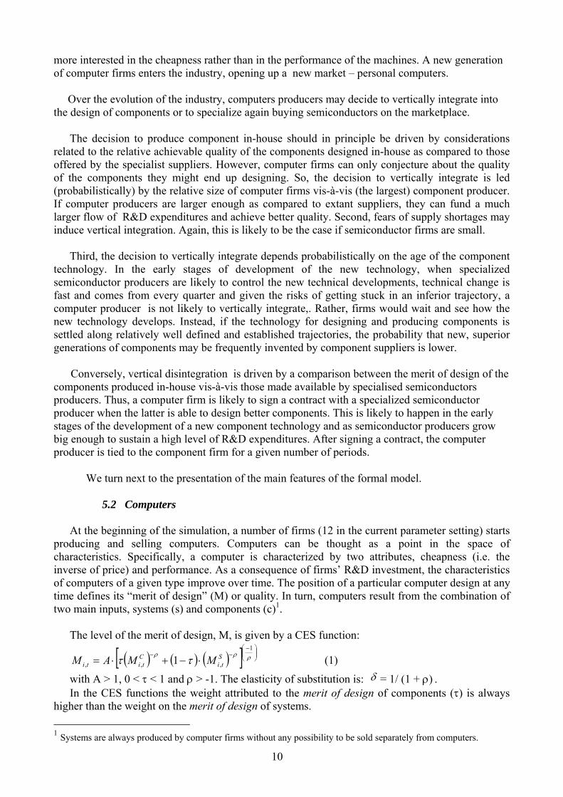
At the beginning of the simulation, a number of firms (12 in the current parameter setting) starts producing and selling computers. Computers can be thought as a point in the space of characteristics. Specifically, a computer is characterized by two attributes, cheapness (i.e. the inverse of price) and performance. As a consequence of firms’ R&D investment, the characteristics of computers of a given type improve over time. The position of a particular computer design at any time defines its “merit of design” (M) or quality. In turn, computers result from the combination of two main inputs, systems (s) and components (c)1.

The level of the merit of design, M, is given by a CES function:

( ) ( ) ( )[ ] ⎟⎟⎠

⎞⎜⎜⎝

⎛ −−−

⋅−+⋅= ρρρττ

1

,,, 1 Sti

Ctiti MMAM (1)

with A > 1, 0 < τ < 1 and ρ > -1. The elasticity of substitution is: δ = 1/ (1 + ρ) . In the CES functions the weight attributed to the merit of design of components (τ) is always

higher than the weight on the merit of design of systems. 1 Systems are always produced by computer firms without any possibility to be sold separately from computers.

10

In the model there are two broadly different types of computers, mainframes (MFs) and personal

computers (PCs). PCs have a comparatively higher weight on components as compared to MF (i.e. τPC > τMF.) and the elasticity of substitution, δ , in PCs is higher than in MF. Similarly, designs of MFs and PCs tend to be located on different rays, or cones, in attribute space, with MFs having a high ratio of performance to cheapness, and PCs having a high ratio of cheapness to performance2.

Different computers are produced by different companies. In other words, a computer company

produces only either mainframe or PCs. Diversification is not contemplated initially in this model. Only in some simulations it will be considered.

5.3 Demand for computers Customers of computers are characterized by their preferences about the two attributes that

define a computer design - performance (z) and cheapness (w). There are two customer groups, one consisting of “big firms” who are especially interested in performance, and care less about cheapness, and the other of “small users” who are especially concerned about cheapness, and who value performance less than do big firms. These differences in preferences show up in terms of how performance and cheapness “trade off” in terms of customer evaluation of merit.

Each customer group consists of a large number of heterogeneous subgroups. Within a

particular subgroup customers – a submarket - buy computers valuing its "merit", compared to other products. The number of submarkets is a parameter of the model. In addition, however, markets are characterized by frictions of various sorts, including imperfect information and sheer inertia in consumers behaviour, brand-loyalty (or lock in) effects as well as sensitiveness to firms' marketing policies. These factors are captured in a compact form by the share of computer brands in overall sub-markets at time t-1: the larger the share of the market that a product already holds, the greater the likelihood that a customer will consider that product. Finally, there is a stochastic element in consumers’ choices between different computers.

Specifically, the “value” that customers attribute to any specific computer design, Mit , of a

computer designed by company i at time t is defined as:

( )δδα −⋅⋅= 1,,, tititi zwM (2)

The probability for computers of firm i to be acquired is applied to each submarket; i.e. every

submarket m selects the computer firm i with a probability ti,Pr . Formally, the “propensity”, Li , of computer i to be sold to a group of customers at time t is

defined as:

11,

1, )1( βα

−+= titi sML (3)

2 The trajectories followed by firms in the space of the characteristics are assumed to be fixed and equal among firms. Given the level of the merit of design for a computer and the slope of the MF and PC trajectories, the values of cheapness (w) and performance (z) that appear into the demand function are defined using the following trigonometric formulas:

titi

titi

Msenz

Mw

,,

,,

)(

)cos(

⋅=

⋅=

β

β

where β indicates an angle express in radian, and is different between PC and MF

11

where is the market share. The probability Pr1, −tis i of the computer i to be sold to a group of

customers at time t is given by:

∑=

iti

titi L

L

,

,,Pr (4)

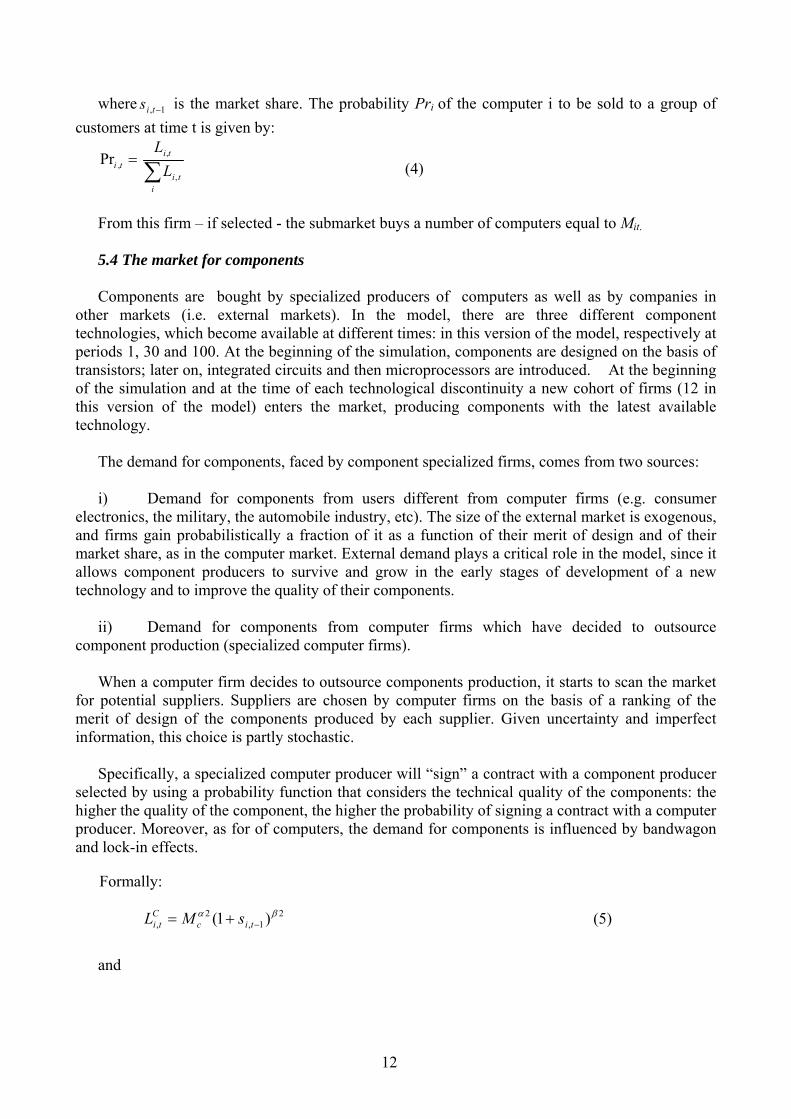
From this firm – if selected - the submarket buys a number of computers equal to Mit. 5.4 The market for components Components are bought by specialized producers of computers as well as by companies in

other markets (i.e. external markets). In the model, there are three different component technologies, which become available at different times: in this version of the model, respectively at periods 1, 30 and 100. At the beginning of the simulation, components are designed on the basis of transistors; later on, integrated circuits and then microprocessors are introduced. At the beginning of the simulation and at the time of each technological discontinuity a new cohort of firms (12 in this version of the model) enters the market, producing components with the latest available technology.

The demand for components, faced by component specialized firms, comes from two sources: i) Demand for components from users different from computer firms (e.g. consumer

electronics, the military, the automobile industry, etc). The size of the external market is exogenous, and firms gain probabilistically a fraction of it as a function of their merit of design and of their market share, as in the computer market. External demand plays a critical role in the model, since it allows component producers to survive and grow in the early stages of development of a new technology and to improve the quality of their components.

ii) Demand for components from computer firms which have decided to outsource component production (specialized computer firms).

When a computer firm decides to outsource components production, it starts to scan the market

for potential suppliers. Suppliers are chosen by computer firms on the basis of a ranking of the merit of design of the components produced by each supplier. Given uncertainty and imperfect information, this choice is partly stochastic.

Specifically, a specialized computer producer will “sign” a contract with a component producer

selected by using a probability function that considers the technical quality of the components: the higher the quality of the component, the higher the probability of signing a contract with a computer producer. Moreover, as for of computers, the demand for components is influenced by bandwagon and lock-in effects.

Formally:

21,

2, )1( βα

−+= ticC

ti sML (5)

and

12

∑= C

ti

CtiC

ti LL

,

,,Pr

(6)

where is the merit of design of the component, LCM it

C is the propensity of component producer i to be selected, is the market share of firm i in the previous period and Pr1, −tis c

i,t is the probability of a supplier to be selected.

A component firm which signs a contract sells a number of components related to the proportion

to which components and systems combine in order to build a computer (in the current parametrization, the proportion is one to one). After signing the contract the computer firm is tied to the component supplier for a certain number of periods, which is a parameter of the model. When this period expires, a new supplier might be selected, using the same procedure, if the firm still decides to buy components on the open market.

The external market is modelled in the same as the computer market, i.e. there is a number of

submarkets to which component firms may sell. A firm gets therefore a fraction of the total value of the external market equal to . C

ti,Pr 5.5 Firms' behaviour and technical progress At the beginning of our story, firms start with a given (randomly drawn) merit of design, they

start to make profits and invest in R&D. Profits, π, are calculated in each period t as: tititititi oqpq ,,,,, ⋅−⋅=π (7) where qit is the number of computers sold, depending on the merit of design level and on the

number of submarkets gained by the firm, p is the price and o is the production cost of a computer. Price is obtained by adding a mark-up, η , to costs:

)1(,, η+⋅= titi op (8) Costs are in turn derived from the merit of design achieved by a computer, considering that the

price of a computer must be equal to the inverse of the achieved cheapness3. The price of components charged by component suppliers is determined symmetrically by adding a fixed mark-up to unit production costs.

Technical progress in components and systems – and hence in computers – is the result of the

R&D activities of computer and semiconductor producers. R&D expenditures are calculated following a simple rule of thumb, i.e. a constant fraction of profits (100% in this version of the

3While the production costs of integrated computer producers are a function of the achieved Mod, the production costs of specialized producers are instead determined as the costs of the system plus the cost of buying the components on the marketplace, i.e. the price charged by the particular supplier from which the computer company is buying. In the model, we assume that an integrated and a specialized firm having the same computer Mod have also the same production costs for a computer. For a given component Mod, the cost of internally produced components is equal to the cost of the externally produced components. The additional costs that would be associated to the mark-up charged by component suppliers and which are “saved” by an integrated firm - are invested in R&D by integrated producers and treated as a cost.

13

model) is invested in R&D in each period. By investing more in R&D, firms buy themselves higher probabilities to increase their merit of design.

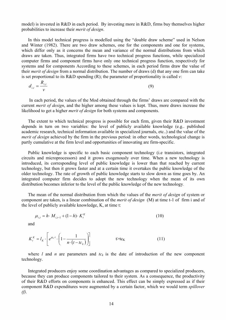
In this model technical progress is modelled using the “double draw scheme” used in Nelson

and Winter (1982). There are two draw schemes, one for the components and one for systems, which differ only as it concerns the mean and variance of the normal distributions from which draws are taken. Thus, integrated firms have two technical progress functions, while specialized computer firms and component firms have only one technical progress function, respectively for systems and for components According to these schemes, in each period firms draw the value of their merit of design from a normal distribution. The number of draws (d) that any one firm can take is set proportional to its R&D spending (R); the parameter of proportionality is called v:

vR

d titi

,, = (9)

In each period, the values of the Mod obtained through the firms’ draws are compared with the

current merit of design, and the higher among these values is kept. Thus, more draws increase the likelihood to get a higher merit of design for both systems and components.

The extent to which technical progress is possible for each firm, given their R&D investment

depends in turn on two variables: the level of publicly available knowledge (e.g.. published academic research, technical information available in specialized journals, etc..) and the value of the merit of design achieved by the firm in the previous period: in other words, technological change is partly cumulative at the firm level and opportunities of innovating are firm-specific.

Public knowledge is specific to each basic component technology (i.e transistors, integrated

circuits and microprocessors) and it grows exogenously over time. When a new technology is introduced, its corresponding level of public knowledge is lower than that reached by current technology, but then it grows faster and at a certain time it overtakes the public knowledge of the older technology. The rate of growth of public knowledge starts to slow down as time goes by. An integrated computer firm decides to adopt the new technology when the mean of its own distribution becomes inferior to the level of the public knowledge of the new technology.

The mean of the normal distribution from which the values of the merit of design of system or

component are taken, is a linear combination of the merit of design (M) at time t-1 of firm i and of the level of publicly available knowledge, K, at time t:

Kttiti KhMh ⋅−+⋅= − )1(1,,µ (10)

and

( ) ⎥⎦

⎤⎢⎣

⎡⎟⎟⎠

⎞⎜⎜⎝

⎛−⋅

−⋅⋅= ⋅

k

tK

Kt tctn

elK k11ϕ t>tcK (11)

where l and n are parameters and tck is the date of introduction of the new component technology.

Integrated producers enjoy some coordination advantages as compared to specialized producers,

because they can produce components tailored to their system. As a consequence, the productivity of their R&D efforts on components is enhanced. This effect can be simply expressed as if their component R&D expenditures were augmented by a certain factor, which we would term spillover (f).

14

So, component R&D -COMPREr

RCi,t - of an integrated computer producer is:

tiC

tiCti RfcR ,,, ⋅+⋅=η (12)

where cC is the cost of its component. cC* η is the difference between the price of component in the open market and its actual cost for the producer. It represents savings gained by self-production. As we mentioned before, we advance the hypothesis that an integrated computer firm allocate these resources to component R&D.

Specialized computer producers invest all their R&D on systems and obviously do not enjoy the

coordination advantages. Component suppliers spend all their R&D on the development of components.

5.6 Vertical Integration and Specialization Computer producers may decide to vertically integrate into semiconductors, if they think that

they can design and produce components that are comparable in quality to those offered by specialist suppliers. In turn, this is more likely to be the case if computer producers are larger enough as compared to extant suppliers, so that they can fund a much larger flow of R&D expenditures. Moreover, the decision to vertically integrate depends probabilistically on the age of the component technology. In the early stages of development of the new technology, when specialized semiconductor producers are likely to control the new technical developments, technical change is fast and comes from every quarter and given the risks of getting stuck in an inferior trajectory, a computer producer is not likely to vertically integrate,. Rather, firms would wait and see how the new technology develops. Instead, if the technology for designing and producing components is settled along relatively well defined and established trajectories, the probability that new, superior generations of components may be frequently invented by component suppliers is lower. Third, fears of supply shortages may induce vertical integration. Again, this is likely to be the case if semiconductor firms are small because the external market for transistor is not too big and/or no dominant firm has emerged.

The probability of integration for each computer firm may be defined, in a compact way, as

follows. Let:

2,

1

, 1;minϑϑ

γ

⎟⎟⎠

⎞⎜⎜⎝

⎛⋅⎟⎟

⎠

⎞⎜⎜⎝

⎛= C

t

titi q

qgA

V (13)

where: Aγ ( γ =TR,IC,MP) = t – (Starting time of Technology γ); qi,t are the sales of the computer

producer; qt C are the sales of the largest component producers and g is a parameter .

Then:

ti

titi V

VbIntegrateob

,

,, 1

)(Pr+

⋅= (14)

where b is a parameter. If the probability of integration is bigger than a number drawn from a uniform distribution (0-1), integration occurs.

The decision to specialize is not symmetrical to the decision to vertically integrate. It is driven

probabilistically by a comparison between the merit of design of the components produced internally and the quality of the best component available on the market.

15

Specifically, the probability of specialization for each firm is defined as follows:

⎟⎟⎠

⎞⎜⎜⎝

⎛ −= 0,

maxmax

,

,, C

ti

Cti

Ct

ti MMM

Z (15)

where max MC is the higher component merit of design available on the market. Then:

ti

titi Z

ZaSpecializeob

,

,, 1

)(Pr+

⋅= (16)

As before, a is a parameter and if Prob(Specialize) is bigger than a number randomly drawn by a uniform distribution, specialization will occur.

A specialized computer firm may also decide to change its supplier, if a better producer has

emerged in the market. The procedure for changing supplier follows the same rule for the specialization process. That is to say, every n periods after the last decision to specialize or the last change of supplier, a specialized firm checks if a better supplier than the current one exists. If this is the case, a new supplier is chosen using the rating mechanism described in the discussion of the demand module.

5.7 Exit Both computer firms and component suppliers exit the market when their market share falls

under a certain minimum threshold. Specifically, the exit rule is defined as follows. For each firm and in each period, the variable

titi seleE ,, )1( ⋅+⋅−= (17) is computed, where l is the inverse of the number of firms active in the market at the beginning

of the simulation (i.e. the market share that would have been held by n equal firms), si,t is the market share of firm i at time t and 0<e<1 is a parameter. Then, if Eit < E, where E is a constant threshold (equal to 0.05 in the current parametrization), the firm exits.

The rule governing the exit of the semiconductor producers is different and simpler. The

probability of exiting of any one firm is an increasing function of the number of consecutive periods in which it does not sell to a computer producer.

6. THE SIMULATION RUNS 6.1 The History-Friendly Simulation The history-friendly simulation has been constructed by applying to the model a

parametrization that reflects the basic assumptions about the processes which would have driven industrial evolution, vertical integration and specialization according to the historical accounts and the interpretative framework discussed earlier.

In the early stages of their evolution, during the transistor period, the two industries experienced

a shake-out and concentration increased. In the computer sector, a company – IBM – soon gained the leadership and an almost monopolistic position. Concentration increased also in the component

16

market, but no firm acquired a clear dominance. The rise of a monopolist in mainframes was sustained by significant “lock-in” effects on the demand side, which magnified early technological advantages and protected the leader from competition. The growth of the leader led quickly to vertical integration, as the large profits of the mainframe producer(s) led to rapid technological advances in their components4. Conversely, semiconductor producers could not exploit large lock-in effects in demand and the extent of the external market was not so big to spur an increase in their size comparable to that experienced by computer producers. Thus, a dominant firm semiconductor company did not emerge and vertical integration of computer firms further reduced the opportunities of growth for semiconductor companies.

When integrated circuits were introduced, new component producers entered the market

mastering the new technology. Computer firms faced, in these circumstances, pressures towards vertical disintegration, to the extent that new component firms were able to produce better components. However, since the external market for semiconductors was still not large enough, specialized component producers remained relatively small and could not innovate as quickly as the computer leaders. Computer companies were also able to adopt integrated circuits technology very quickly and thus they ended up producing in house again their own components5.

The third technological discontinuity – microprocessors – involved instead different conditions.

First, the new cohort of component producers could benefit from a much larger external market and could then invest more in R&D. Thus, they could grow quickly and achieve high levels of quality.

Second, lock-in effects in the demand for components – both in the computer market and in the

external market - are much more significant in the case of microprocessors as compared to integrated circuits and transistors. As a consequence, a dominant component producer emerges in this era.

Third, the introduction of microprocessors marks a sharp technological discontinuity, which

allowed to design much better components than those based on integrated circuits. Thus, the new entrants can supply vastly superior products and catching up by integrated mainframe producers was slower.

Fourth, microprocessors make it possible to design and start selling a new – previously

unattainable – type of computers, i. e. personal computers. PCs differ from mainframes – in the language of this model – in two important respects. The weight of components with respect to systems is much higher in determining the Mod of the computer as compared to mainframes. Moreover, PCs are much cheaper than mainframes. Thus, a whole new class of customers, who attribute much more value to cheapness than to performance, started buying the new type of computers: the PC market opened up and grew rapidly. PC producers, however, were relatively small as compared to the microprocessor suppliers, who could also sell to a large external market. Thus, quite soon large specialized microprocessor suppliers began to emerge before any of the new producers of PCs became very large.

4 Moreover, these benefits of vertical integration was reinforced by the advantages of designing jointly components

and systems. 5 In the history of the computer history, one further reason that led IBM to vertically integrate into the production of

integrated circuits was the risk of supply shortages. Producers of integrated circuits were too small to guarantee a steady and safe supply of components on the scale needed to satisfy IBM demand. A module of the model takes this issue into account. It is assumed that the production of components might be constrained by the productive capacity of semiconductor firms: specifically, capacity constraints manifest themselves in an erosion of the firm’s component mod, reflecting a decrease in the quality of the component, due for example, to delivery delays, etc.. Lower component quality feeds back on sales, profits and R&D expenditures. After capacity constraints have been experienced, firms gradually adjust their capacity drawing from their profits (and therefore decreasing correspondingly their R&D). This module, however, is not active in the current version of the model.

17

Fifth, lock-in effects on the demand side are less important in the case of PCs as compared to

mainframes: hence, no PC producer could establish and maintain a dominant position becoming large enough to make vertical integration reasonable. As a result, PC computer firms remained specialized in systems. And a dominant microprocessor supply firm emerged. The rise of strong and large microprocessor firms, selling their wares on a large but competitive PC market, soon made it costly and risky for mainframe producers to continue to design and produce their own microprocessors6. This led to vertical disintegration also in the mainframe industry.

In sum, the history-friendly simulation is based on the following assumptions on the relevant

variables and parameters and on their values: - the size of the external market is relatively small in the case of transistors and integrated

circuits and significantly higher for microprocessors; - lock-in effects in demand are very important for mainframes and much less so for both

PCs and components; - demand for microprocessors is subject to much stronger lock-in effects as compared to

transistors and integrated circuits; - the introduction of microprocessors allows much higher improvements in component

designs as compared to the older technology: this technological discontinuity is much sharper than the previous one.

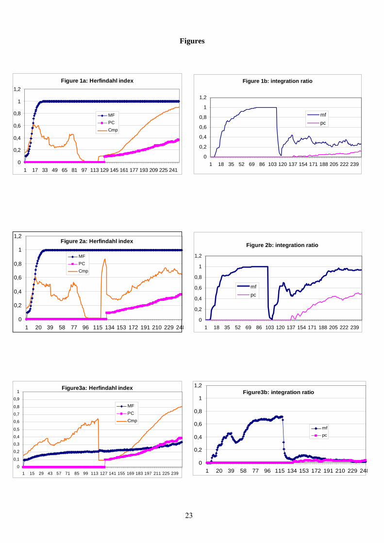
// FIGURE 1 ABOUT HERE // Under this parametrization, the simulation replicates the key aspects of the story. Figure 1 – as

well as the subsequent figures for the other exercises – reports the averages over 100 runs. A dominant firm emerges quickly in the mainframe industry and tends to become vertically integrated relatively early. In the semiconductor industry, concentration rises as demand from computer producers and – less sharply – from the external market exert selective pressures and firms leave the market7. At the time of the introduction of integrated circuits, new semiconductor companies enter the market and concentration drops sharply. However, the dominant mainframe firm remains vertically integrated, because the external market is not large enough to sustain a significant growth of the new entrants and of the quality of their components. The absence of a demand from the mainframe producer induces a sharp shakeout and concentration gradually begin to increase again in the semiconductor market. When vertical integration is complete in the computer market, the semiconductor producers are left with no demand and exit this market. As a consequence, concentration falls to zero.

The third technological discontinuity sets in motion a different story. Microprocessors constitute

a major technological advance as compared to integrated circuit and a large external market supports a significant improvement in the quality of the new components. Moreover, the PC market opens up, generating a substantial new demand and fuelling further advances in the merit of the components. As a consequence, the computer leader decides to specialize, adding a new large demand. Finally, lock-in effects in the demand for microprocessors are now significant. Hence, a dominant firm emerges also in the semiconductor market. The establishment of a monopoly in the supply of components contributes however to maintain competition in the PC market, since all firms get their microprocessors from the same source: concentration increases but no firm comes actually to dominate the market. In the last periods of the simulation, as the microprocessors technology matures, the incentives towards specialization become slightly less compelling and, in 6 Furthermore, the advantages of tailoring microprocessor design to systems design were less prominent for PCs than

they had been for mainframes, a fortiori reducing the possible advantages of integration. 7 The Herfindahl index for component producers is computed with reference to the computer market only

18

some simulations, the mainframe firm and some PC producers decide to vertically integrate. 6.2 Testing the model: counterfactuals In order to check the logical consistency of the model and its sensitivity to changes in key

parameters, we run some counterfactual simulations. Specifically, we change the values of the parameters of the variables which, according to our assumptions, generate the history-friendly run.

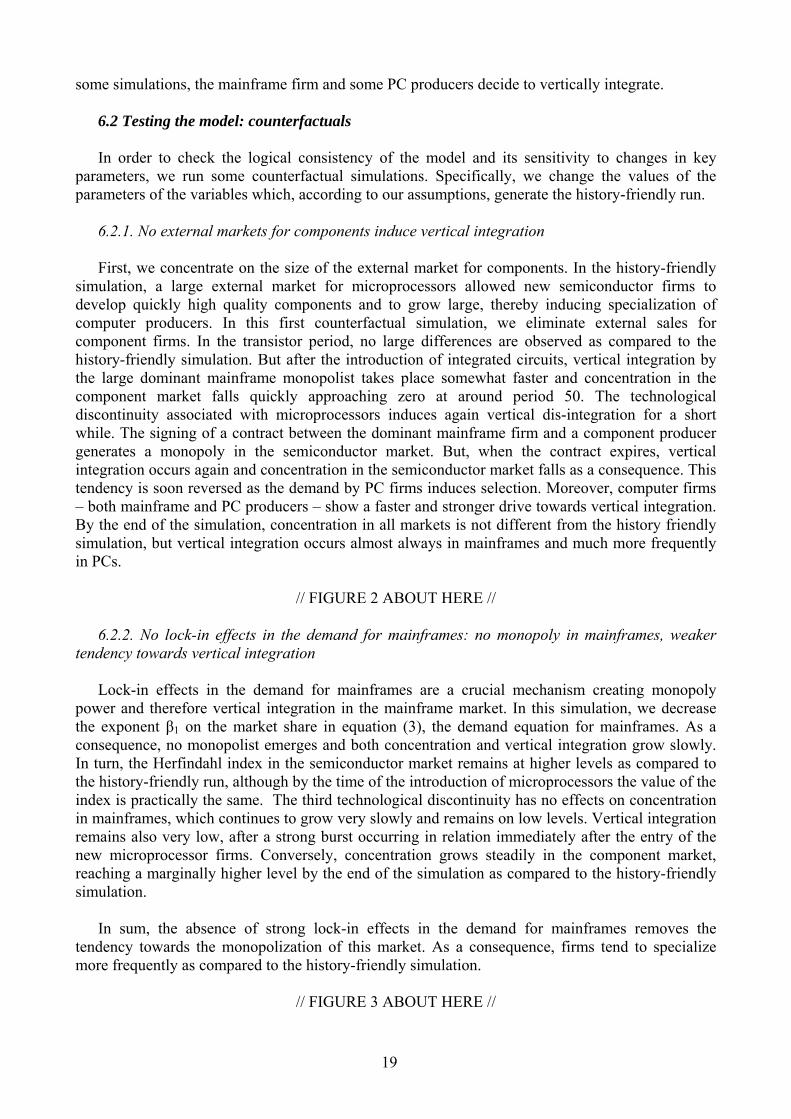
6.2.1. No external markets for components induce vertical integration First, we concentrate on the size of the external market for components. In the history-friendly

simulation, a large external market for microprocessors allowed new semiconductor firms to develop quickly high quality components and to grow large, thereby inducing specialization of computer producers. In this first counterfactual simulation, we eliminate external sales for component firms. In the transistor period, no large differences are observed as compared to the history-friendly simulation. But after the introduction of integrated circuits, vertical integration by the large dominant mainframe monopolist takes place somewhat faster and concentration in the component market falls quickly approaching zero at around period 50. The technological discontinuity associated with microprocessors induces again vertical dis-integration for a short while. The signing of a contract between the dominant mainframe firm and a component producer generates a monopoly in the semiconductor market. But, when the contract expires, vertical integration occurs again and concentration in the semiconductor market falls as a consequence. This tendency is soon reversed as the demand by PC firms induces selection. Moreover, computer firms – both mainframe and PC producers – show a faster and stronger drive towards vertical integration. By the end of the simulation, concentration in all markets is not different from the history friendly simulation, but vertical integration occurs almost always in mainframes and much more frequently in PCs.

// FIGURE 2 ABOUT HERE //

6.2.2. No lock-in effects in the demand for mainframes: no monopoly in mainframes, weaker

tendency towards vertical integration Lock-in effects in the demand for mainframes are a crucial mechanism creating monopoly

power and therefore vertical integration in the mainframe market. In this simulation, we decrease the exponent β1 on the market share in equation (3), the demand equation for mainframes. As a consequence, no monopolist emerges and both concentration and vertical integration grow slowly. In turn, the Herfindahl index in the semiconductor market remains at higher levels as compared to the history-friendly run, although by the time of the introduction of microprocessors the value of the index is practically the same. The third technological discontinuity has no effects on concentration in mainframes, which continues to grow very slowly and remains on low levels. Vertical integration remains also very low, after a strong burst occurring in relation immediately after the entry of the new microprocessor firms. Conversely, concentration grows steadily in the component market, reaching a marginally higher level by the end of the simulation as compared to the history-friendly simulation.

In sum, the absence of strong lock-in effects in the demand for mainframes removes the

tendency towards the monopolization of this market. As a consequence, firms tend to specialize more frequently as compared to the history-friendly simulation.

// FIGURE 3 ABOUT HERE //

19

6.2.3. No lock-in effects in the semiconductor market: lower concentration in the microprocessors market

In these runs, lock-in effects in the semiconductor market are eliminated. This change produces

no effects in the transistor and integrated circuits eras, where vertical integration of computer firms implies a very small demand for components and hence little room for the lock-in effect to exert its impact. Instead concentration in the microprocessors market decreases significantly as compared to the history-friendly simulation. The vertical scope of computer firms remains unsurprisingly unchanged, given that specialization occurred also in the history-friendly run.

// FIGURE 4 ABOUT HERE //

6.2.4 Microprocessors are not a drastic technological revolution: vertical integration and

higher concentration in the microprocessors and PC markets In the history-friendly simulation, the introduction of microprocessors implied a significant

increase in the merit of design of components and much higher scope for improvement. In these runs, the magnitude of this discontinuity is reduced, by decreasing the value of the initial merit of design of microprocessors. The consequences are dramatic. Mainframe and (to a lesser extent) PC firms now tend to vertically integrate. Concentration increases in the component market, since very few component firms survive. Vertical integration induces also higher concentration in the PC market, because now PC firms develop their own components instead of buying them from external suppliers.

// FIGURE 5 ABOUT HERE //

7. Conclusion The model is able to reproduce the main stylized facts of the patterns of competition and vertical

integration in the computer and semiconductor industries and in responding to changes in the key parameters in the counterfactual experiments.

The model illustrates how the patterns of vertical integration and specialization in the computer

industry change as a function of the evolving levels and distribution of firms’ capabilities over time and – more generally – how they depend on the co-evolution of the upstream and downstream sector. Specific conditions in each of these markets – i.e. the size of the external market, the magnitude of the technological discontinuities, the lock-in effects in demand – exert critical effects and feedbacks on market structure and on the vertical scope of firms as time goes by.

Clearly, these exercises are preliminary. Immediate future work requires a much more extensive

and deeper analysis of the properties of the model .

20

References Arora A. Bokhari F. (2000) Vertical integration and dynamics and industry evolution

Carnegie Mellon University Mimeo Bresnahan T.F., Malerba F. (1999), Industrial Dynamics and the Evolution of Firms’ and

Nations’ Competitive Capabilities in the World Computer Industry, in D. Mowery and R.Nelson (ed) The Sources of Industrial Leadership Cambridge University Press

W.A. Brock (1999), “Scaling in Economics: A Reader’s Guide”, Industrial and Corporate Change, 8,3, 409-446

F. Chiaromonte and G. Dosi (1992), “The Microfoundations of Competitiveness and Their Macroeconomic Implications”, in C. Freeman and D. Foray (eds.), Technology and the Wealth of Nations, Pinter Publishers, London.

Cohen W. Malerba F. “Is the tendency to variation a chief source of progress?” Industrial and Corporate Change n.3, 2001

Christensen, C. and Rosenbloom, R. (1994), Technological Discontinuities, Organizational Capabilities, and Strategic Commitments, Industrial and Corporate Change,3

H. Dawid, and M. Reimann (2005), Diversification: A Road to Ineffciency in Product Innovations? Department of Business Administration and Economics and Institute of Mathematical Economics, University of Bielefeld, mimeo.

G. Dosi, S. Fabiani, R. Aversi and M. Meacci (1994), The Dynamics of International Differentiation: A Multi-Country Evolutionary Model, Industrial and Corporate Change, 3, 1, 225-242

Dosi, G., Marsili O., Orsenigo L. and Salvatore R. (1995), “"Technological Regimes, Selection and Market Structures", Small Business Economics.

Jacobides M. and S.G. Winter (2004), The coevolution of capabilities and transaction costs: explaining the institutional structure of production Strategic management Journal forthcoming

B. Jovanovic and G.M. MacDonald (1993), The Life Cycle of a Competitive Industry”, Working paper No. 4441, National Bureau of Economic Research, Cambridge (Ma).

Klepper, S. (1996), "Entry, Exit and Innovation over the Product Life Cycle", American Economic Review, 86. no.3, 562-582.

Kricks G. (1995) “Vertical integration in the mainframe computer industry: a transaction cost interpretation” Journal of Economic Behavior and Organization n.26, 75/91

Langlois R.N.(1992), Transaction Cost Economics in Real Time, Industrial and Corporate Change

Langlois R. N., Robertson P. L. (1996), Firms Markets and Economic Change: a Dynamic Theory of Business Institutions, Routledge, London

Malerba F. (1985) The Semiconductor Business, University of Wisconsin Press, F. Pinter London.

Malerba F. Nelson R. Orsenigo L. Winter S. (1999) History friendly models of industry evolution: the computer industry Industrial and Corporate Change, 1 pag.3-41

Malerba F. Nelson R. Orsenigo L. Winter S. (2005), The Dynamics of the Vertical Scope of Firms in related Industries: the Co-evolution of Competences, Technological Change and the Size and Structure of Markets, mimeo

Mowery D. (ed.) (1996), The International Computer Software. A Comparative Study of Industry Evolution and Structure, Oxford University Press, Oxford

Nelson R.(1994),The Co-evolution of Technology, Industrial Structure, and Supporting Institutions, Industrial and Corporate Change, pag. 47-63

21

Nelson, R. R., and S. G. Winter. 1982. An Evolutionary Theory of Economic Change. The Belknap Press of Harvard University Press: Cambridge, MA.

Smith A. (1776), The Wealth of Nations. Stigler G. (1951), The division of labour is limited by the extent of the market Journal of

Political Economy Teece D. J. (1986), Profiting from Technological Innovation, Research Policy Teece D.J., Pisano G.P. (1994), The Dynamic Capabilities of Firms: an Introduction,

Industrial and Corporate Change Teece D.J., Pisano G., Shuen A.(1992), Dynamic Capabilities and Strategic Management,

Working Paper Teece, D.J., R. Rumelt, G. Dosi and S. Winter. 1994. Understanding Corporate Coherence:

Theory and Evidence. Journal of Economic Behavior and Organization 23: 1-30. Utterback, J.M and W. Abernathy. 1975. A Dynamic Model of Process and Product

Innovation. OMEGA. 3: 639-655. Williamson O. (1975), Markets and Hierarchies, The Free Press, New York Winter S. (1984), Schumpeterian Competition in Alternative Technological Regimes,

Journal of Economic Behavior and Organization Winter S.(1987), Knowledge and Competence as Strategic Assets, in Teece D. J. The

competitive Challenge, Cambridge (Mass), Ballinger, pag 159-184 Winter S., Kaniovski Y. And Dosi G. (1999), “Modeling Industrial Dynamics with

Innovative Entrants”, mimeo

22

Figures

Figure 1a: Herfindahl index

0

0,2

0,4

0,6

0,8

1

1,2

1 17 33 49 65 81 97 113 129 145 161 177 193 209 225 241

MFPCCmp

Figure 1b: integration ratio

0

0,2

0,4

0,6

0,8

1

1,2

1 18 35 52 69 86 103 120 137 154 171 188 205 222 239

mfpc

Figure 2a: Herfindahl index

0

0,2

0,4

0,6

0,8

1

1,2

1 20 39 58 77 96 115 134 153 172 191 210 229 248

MFPCCmp

Figure 2b: integration ratio

0

0,2

0,4

0,6

0,8

1

1,2

1 18 35 52 69 86 103 120 137 154 171 188 205 222 239

mfpc

Figure3a: Herfindahl index

0

0,1

0,2

0,3

0,4

0,5

0,6

0,7

0,8

0,9

1

1 15 29 43 57 71 85 99 113 127 141 155 169 183 197 211 225 239

MFPCCmp

Figure3b: integration ratio

0

0,2

0,4

0,6

0,8

1

1,2

1 20 39 58 77 96 115 134 153 172 191 210 229 248

mfpc

23

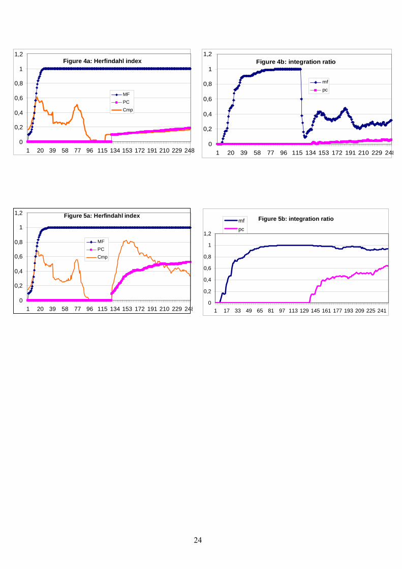
Figure 4b: integration ratio

0

0,2

0,4

0,6

0,8

1

1,2

1 20 39 58 77 96 115 134 153 172 191 210 229 248

mfpc

Figure 5a: Herfindahl index

0

0,2

0,4

0,6

0,8

1

1,2

1 20 39 58 77 96 115 134 153 172 191 210 229 248

MFPCCmp

Figure 5b: integration ratio

0

0,2

0,4

0,6

0,8

1

1,2

1 17 33 49 65 81 97 113 129 145 161 177 193 209 225 241

mfpc

1,2 Figure 4a: Herfindahl index

1

0,8 MF

0,6 PC

0,4

0,2

0 1 20 39 58 77 96 115 153 172 191 134 210 229 248

Cmp

24

Appendix We provide here a complete list of the notation used in the model Indices:

• i index for firms, { }Ii ,..,1=• t index for time periods, { }Tt ,...,1=• mf, pc, tr, ic, mp indices for type of firm

General model parameters:

• T = 250 time horizon • tc date of introduction of a new component technology : tcTR = 1

tcIC = 40 tcMP = 120

• TPC = 130 date of introduction of PC producers Exogenous industry characteristics:

• I = 12 number of firms • submMF = 100 initial number of submarkets for MF firms • submPC = 100 initial number of submarkets for PC firms • EMTR = 8 initial number of external market submarkets for transistors producers • EMIC = 8 initial number of external market submarkets for integrated circuits producers • EMMP = 1050 initial number of external market submarkets for microprocessors producers • Lcont = 8 contract length • Lintmin = 16 minimum length of vertical integration • α1MF = 1 weight of merit of design on Li,t • α1PC = 1 weight of merit of design on Li,t • β1MF = 6 bandwagon effect for mainframes • β1PC = 1 bandwagon effect for personal computers • α2 =1 weight of merit of design on Li.t

C • β2 = 6 bandwagon effect for semiconductors producers • hmf = 0.75, hpc = 0.75, hcmp = 0.75, weight of merit of design when calculating µi,t • Kt level of public knowledge at time t • limMF = 2, limPC = 2, limTR = 2, limIC =1.12, limMP =1.78 coefficient for public knowledge

function • φSYS = 0.01, φTR = 0.01, φIC = 0.015, φMP = 0.02 rates of growth of public knowledge • θ1 = 1 parameter indicating the rapidity by which a type of component become obsolete

when defining the integration probability. • θ2 = 1 parameter indicating the importance of qi,t relatively to qt C when defining the

integration probability • g = 20 age of technology divider • b = 1 coefficient for integration probability function • a = 1 coefficient for specialization probability function • E = 0.05 minimum threshold of market share necessary to survive • e = 0.3 weight given to market share in the exit rule

Endogenous industry characteristics: • Aγ age of technology γ at time t

Exogenous firm characteristics:

25

• MCTR,0 = 0.959, MC

IC,0 = 2, MCIC,0 = 25 initial value of merit of design for each kind of

semiconductor • MMF,0 = 0.959, MPC,0 = 3.6692 initial value of merit of design for mainframes and pc. • τMF = 0.5, τPC = 0.75 weight of component merit of design on the whole computer merit

of design • A = 1 coefficient for CES function • ρMF = -0.5, ρPC = -0.75 degree of substitutability of the inputs in the CES function • α = 1 coefficient for the function that indicates the “value” that customers attribute to any

specific computer design • δMF = 0.3, δPC= 0.7 weight given to cheapness, depending on the type of costumer • η = 0.1 mark-up added to costs • λmf = 0.6, λpc= 0.6 mod replication capability when vertical integration takes place • vMF = 250, vPC = 250, vTR = 200, vIC = 250, vMP = 500 draw costs for each kind of firm • f mf= 0.1, f pc= 0.1 spillover that enhance the RD efforts of an integrated firm

Endogenous firm characteristics:

• Mi,t merit of design of a computer produced by firm i at time t • Mi,t

C merit of design of a component produced by firm i at time t • Mi,t

S merit of design of a system produced by firm i at time t • wi,t value of cheapness of computer i at time t • zi,t value of performance of computer i at time t • Li,t propensity of the computer i to be sold to a group of customers at time t • Pri,t probability of the computer i to be sold to a group of customers at time t • si,t market share of firm i at time t • Li.t

C propensity of a component producer i to be selected at time t • PrC

i,t probability of a supplier i to be selected at time t • pi,t price of a computer/component produced by firm i at time t • πi,t profits of firm i at time t • oi,t production cost of firm i at time t • di,t number of draws of firm i at time t • Ri,t RD spending of firm i at time t • RC

i,t RD spending of an integrated firm i at time t • µi,t mean of the normal distribution from which the values of the merit of design of system or

component are taken • qi,t sales of a computer firm i at time t • qt C sales of the largest component producers at time t • Vi.t integration probability of firm i at time t • Zi,t specialization probability of firm i at time t • Ei,t variable compared to the minimum constant threshold of market share E necessary to

survive in the market

26

The reported results for the relevant variables on which we concentrate our attention

(concentration indexes, the extent of vertical integration and/or specialization, rates of technological change) are the means of extensive Monte Carlo exercises8.

Moreover, following Dawid et al (2005), we carried on sensitivity analysis on the model by

generating 100 different profiles of the key model parameters. The profiles were generated randomly, where each parameter was drawn from a uniform distribution bounded by a conceptually plausible range. Each particular setting for our control parameters was run over all 100 profiles and the results obtained were averaged over these runs. As an additional robustness check we repeated the procedure with another 100 random profiles in the same manner and tested several of our qualitative insights obtained with the initial set of profiles. In all these cases our findings were confirmed by such a check. Summarizing, all the results were found to be very robust under the settings we discussed above, namely 100 distinctly different runs, with profiles based on parameter ranges that were determined by plausibility checks beforehand . In Table 1 we list the parameters that have been used for sensitivity and robustness analysis, together with their respective ranges given by upper and lower bounds for their values. For each of the 100 profiles we generated, these parameters were independently, uniformly random drawn between these bounds. In Table 2 we show the results related to this random parameter setting. Table 1

Parameter Lower Bound Upper Bound Parameter Lower Bound Upper Bound

Lcont 6 10 MCTR,0 0.5 1.5

Lintmin 14 18 MCIC,0 1 3

β1MF 5 7 MCMP,0 23 27

β1PC 0 2 fmf 0 0.2 α1MF 0.5 1.5 fpc 0 0.2 α1PC 0.5 1.5 λmf 0.4 0.8 β2 5 7 λpc 0.4 0.8 hmf 0.65 0.85 hpc 0.65 0.85 hcmp 0.65 0.85

EMTR EMIC

6 6

10 10

g 18 22 EMMP 1000 1100

8 The Monte Carlo variance of these variables is typically negligible. This allows us to avoid reporting confidence

intervals.

27

Table 2

herfindahl index (random par)

0

0,2

0,4

0,6

0,8

1

1,2

1 19 37 55 73 91 109 127 145 163 181 199 217 235

MFPCCmp

integration ratio (random par)

0

0,2

0,4

0,6

0,8

1

1,2

1 18 35 52 69 86 103 120 137 154 171 188 205 222 239

mfpc

28