a higher order accurate finite element method for viscous compressible flows
TRANSCRIPT

8/8/2019 A Higher Order Accurate Finite Element Method for Viscous Compressible Flows
http://slidepdf.com/reader/full/a-higher-order-accurate-finite-element-method-for-viscous-compressible-flows 1/86
A HIGHER ORDER ACCURATE FINITE ELEMENT METHOD FOR
VISCOUS COMPRESSIBLE FLOWS
by
Daryl Lawrence Bonhaus
Dissertation submitted to the Faculty of the
Virginia Polytechnic Institute and State University
in partial fulfillment of the requirements for the degree of
DOCTOR OF PHILOSOPHY
in
Aerospace and Ocean Engineering
APPROVED:
Bernard Grossman, Chairman
This research was conducted at NASA LaRC.
W. Kyle Anderson
Robert Walters
Joseph Schetz
William Mason
November, 1998Blacksburg, VA
8/8/2019 A Higher Order Accurate Finite Element Method for Viscous Compressible Flows
http://slidepdf.com/reader/full/a-higher-order-accurate-finite-element-method-for-viscous-compressible-flows 2/86
A HIGHER ORDER ACCURATE FINITE ELEMENT METHOD FOR VISCOUS
COMPRESSIBLE FLOWS
by
Daryl L. Bonhaus
Committee Chairman: Bernard Grossman
Aerospace and Ocean Engineering
(ABSTRACT)
The Streamline Upwind/Petrov-Galerkin (SU/PG) method is applied to higher-order
finite-element discretizations of the Euler equations in one dimension and the Navier-
Stokes equations in two dimensions. The unknown flow quantities are discretized on
meshes of triangular elements using triangular Bezier patches. The nonlinear residual
equations are solved using an approximate Newton method with a pseudotime term. The
resulting linear system is solved using the Generalized Minimum Residual algorithm with
block diagonal preconditioning.
The exact solutions of Ringleb flow and Couette flow are used to quantitatively
establish the spatial convergence rate of each discretization. Examples of inviscid flows
including subsonic flow past a parabolic bump on a wall and subsonic and transonic flows
past a NACA 0012 airfoil and laminar flows including flow past a a flat plate and flow past
a NACA 0012 airfoil are included to qualitatively evaluate the accuracy of the discretiza-
tions. The scheme achieves higher order accuracy without modification. Based on the test
cases presented, significant improvement of the solution can be expected using the higher-
order schemes with little or no increase in computational requirements. The nonlinear sys-
tem also converges at a higher rate as the order of accuracy is increased for the same num-
ber of degrees of freedom; however, the linear system becomes more difficult to solve.
Several avenues of future research based on the results of the study are identified, includ-
ing improvement of the SU/PG formulation, development of more general grid generation
strategies for higher order elements, the addition of a turbulence model to extend the
method to high Reynolds number flows, and extension of the method to three-dimensional
flows. An appendix is included in which the method is applied to inviscid flows in three

8/8/2019 A Higher Order Accurate Finite Element Method for Viscous Compressible Flows
http://slidepdf.com/reader/full/a-higher-order-accurate-finite-element-method-for-viscous-compressible-flows 3/86
iii
dimensions. The three-dimensional results are preliminary but consistent with the findings
based on the two-dimensional scheme.

8/8/2019 A Higher Order Accurate Finite Element Method for Viscous Compressible Flows
http://slidepdf.com/reader/full/a-higher-order-accurate-finite-element-method-for-viscous-compressible-flows 4/86
iv
Acknowledgments
I am grateful for the assistance of Dr. Mark H. Carpenter for valuable technical dis-
cussions and a review of this manuscript. I am also grateful to Christian Whiting for help-
ful discussions during his visits to the Langley Research Center and to Dr. Thomas W.
Roberts for many helpful discussions.
I would particularly like to thank Dr. W. Kyle Anderson, who has been both a friend
and a mentor to me throughout my career.

8/8/2019 A Higher Order Accurate Finite Element Method for Viscous Compressible Flows
http://slidepdf.com/reader/full/a-higher-order-accurate-finite-element-method-for-viscous-compressible-flows 5/86
v
Table of Contents
Abstract ii
Acknowledgments iv
Table of Contents v
List of Figures vii
Chapter 1 Introduction 1
Chapter 2 The Streamline Upwind/Petrov-Galerkin Method 6
2.1 Scalar Advection - One Dimension .....................................................................6
2.2 Advective Systems - One Dimension ..................................................................82.3 Scalar Advection - Multiple Dimensions .............................................................9
2.4 Advective Systems - Multiple Dimensions ........................................................10
Chapter 3 Quasi-One-Dimensional Euler Equations 11
3.1 Governing Equations .........................................................................................11
3.2 Finite Element Formulation ...............................................................................12
3.3 Solution Methodology .......................................................................................13
3.4 Results ................................................................................................................15
Chapter 4 Two-Dimensional Navier-Stokes Equations 22
4.1 Governing Equations .........................................................................................22
4.2 Finite Element Formulation ...............................................................................25
8/8/2019 A Higher Order Accurate Finite Element Method for Viscous Compressible Flows
http://slidepdf.com/reader/full/a-higher-order-accurate-finite-element-method-for-viscous-compressible-flows 6/86
vi
4.3 Solution Methodology .......................................................................................27
4.3.1 Discretization .........................................................................................27
4.3.2 Solution Procedure .................................................................................30
4.4 Inviscid Flow Results .........................................................................................32
4.4.1 Ringleb Flow ..........................................................................................32
4.4.2 Bump on a Wall .....................................................................................34
4.4.3 NACA 0012 Airfoil ...............................................................................34
4.5 Laminar Viscous Flow Results ..........................................................................36
4.5.1 Couette Flow ..........................................................................................36
4.5.2 Flat Plate ................................................................................................37
4.5.3 NACA 0012 Airfoil ...............................................................................38
Chapter 5 Concluding Remarks 59
References 62
Appendix A Three-Dimensional Euler Equations 69
A.1 Governing Equations .........................................................................................69
A.2 Finite Element Formulation ..............................................................................70
A.3 Solution Methodology ......................................................................................70
A.4 Results ...............................................................................................................74
5.0.1 NACA 0012 Wing .................................................................................74
5.0.2 ONERA M6 Wing .................................................................................74
Vita 78

8/8/2019 A Higher Order Accurate Finite Element Method for Viscous Compressible Flows
http://slidepdf.com/reader/full/a-higher-order-accurate-finite-element-method-for-viscous-compressible-flows 7/86
vii
List of Figures
1. Pressure error for converging-diverging nozzle with purely subsonic flow..................19
2. Pressure error for converging-diverging nozzle with supersonic exit flow...................20
3. Pressure error for converging-diverging nozzle flow with a standing shock. ...............21
4. Element data distribution using triangular Bezier patches. ...........................................40
5. Boundary element data distribution using Bezier segments..........................................41
6. Computational regions in Ringleb flow domain used for analysis. ...............................42
7. Generation of finite element meshes for Ringleb flow..................................................43
8. Error norms in subsonic region of Ringleb flow. ..........................................................44
9. Error norms in supersonic region of Ringleb flow. .......................................................45
10. Geometry and grid for parabolic bump in a channel. ..................................................46
11. Surface Mach number distribution for parabolic bump in a channel...........................47
12. Mach number contours for parabolic bump on a wall.................................................48
13. Fine grid for inviscid flow over a NACA 0012 airfoil. ...............................................49
14. Surface pressure distribution for subcritical NACA 0012 airfoil. ...............................50
15. Surface pressure distribution for transonic NACA 0012 airfoil. .................................51
16. Solution domain for rotational Couette flow. ..............................................................52
17. Error in circumferential velocity for rotational Couette flow......................................5318. Solution domain and baseline grid for flat plate flow..................................................54
19. Skin friction distributions for flat plate flow. ..............................................................55
20. Sample grid for laminar flow over a NACA 0012 airfoil. ...........................................56
21. Skin friction distributions for laminar flow over a NACA 0012 airfoil. .....................57

8/8/2019 A Higher Order Accurate Finite Element Method for Viscous Compressible Flows
http://slidepdf.com/reader/full/a-higher-order-accurate-finite-element-method-for-viscous-compressible-flows 8/86
viii
22. Convergence histories for laminar flow over a NACA 0012 airfoil............................58
23. Element data distribution using triangular Bezier patches. .........................................75
24. Mid-span surface pressure distribution for NACA 0012 wing....................................76
25. Surface pressure distribution for ONERA M6 wing at 65% span. ..............................77
8/8/2019 A Higher Order Accurate Finite Element Method for Viscous Compressible Flows
http://slidepdf.com/reader/full/a-higher-order-accurate-finite-element-method-for-viscous-compressible-flows 9/86
1
Chapter 1
Introduction
High-Reynolds-number Navier-Stokes computations for complex aerodynamic con-figurations currently require vast amounts of computer resources for adequate resolution
of the flow field. Indeed, the demands are so great that it is often not possible to perform
complete and rigorous grid convergence studies for these configurations. State-of-the-art
methods rely on linear data distributions in mesh cells resulting in at best second order
accuracy. Methods based on higher order data distributions introduce additional computa-
tional complexity, but yield more accurate results, especially as the mesh is refined.
Higher order methods have the potential to achieve solutions of much higher quality on
coarser meshes compared to present state-of-the-art methods.
One of the most popular schemes for obtaining solutions on unstructured meshes is
the finite volume scheme, in which the governing equations are solved in integral form
over the discrete volumes formed by the cells of a mesh. Descriptions of various finite-vol-
ume schemes on unstructured meshes are given by Barth and Jesperson[1], Whitaker, et
al.[2], Jameson, et al.[3, 4, 5], and Mavriplis and Jameson[6]. Barth[7] presents a detailed
account of the implementation of finite volume schemes for the Euler and Navier-Stokes
equations using efficient edge-based data structures. Finite volume schemes generally
solve for quantities averaged over cells of the actual mesh in the case of cell-centered
schemes or over cells of a dual mesh in the case of vertex schemes. In any event, in order
to evaluate the residual, a polynomial data distribution must be reconstructed from these
8/8/2019 A Higher Order Accurate Finite Element Method for Viscous Compressible Flows
http://slidepdf.com/reader/full/a-higher-order-accurate-finite-element-method-for-viscous-compressible-flows 10/86
2
averaged quantities.
To achieve second order accuracy (as in the foregoing references), a linear distribu-
tion can be reconstructed in a cell using data from the cell’s immediate neighbors. In con-
trast, to achieve higher than second order accuracy, a higher order distribution must be
constructed in each cell, requiring information from more distant neighbors. This was
done by Barth and Frederickson[8] for quadratic reconstruction (and hence third order
accuracy). More recently, Hu and Shu[9] devised a fourth order scheme without expand-
ing the third order stencil by requiring averaged quantities to match in all cells of the sten-
cil. While these methods show promising results, extending them to even higher order
accuracy will require further expansion of the stencil to still more distant neighboring
cells. These stencils will be nonsymmetric in general and the reconstruction indices and
coefficients must be stored for every cell in contrast to finite-element methods, in which
interpolation coefficients are identical in every cell.
Halt[10] and Halt and Agarwal[11] used a variation of a finite volume scheme in
which higher order polynomial data distributions were constructed locally in each cell
using cell-averaged derivative information. To solve for the cell-averaged derivatives, the
governing equations were extended to include either derivatives or moments of the gov-
erning equations. Halt demonstrated that significant gains in accuracy as well as efficiency
could be achieved through the use of higher order methods. Halt also concluded that using
moments of the governing equations was more robust than using the derivative method.
Halt’s moment method is similar to the Discontinuous Galerkin finite-element method
described later in this chapter.
An alternative to the finite-volume formulation is the finite-element method. In this
case, a polynomial data distribution is prescribed in each cell rather than reconstructing
the distribution from averaged quantities. Finite element theory is described in detail by
Zienkiewicz[12], Hughes[13], and Baker and Pepper[14]. In this method, the governing
equations are solved in weak form by forming an inner product of the residual and a set of
“trial” functions. As with finite difference and finite volume schemes, care must be taken
to produce a stable scheme for the Euler and Navier-Stokes equations.

8/8/2019 A Higher Order Accurate Finite Element Method for Viscous Compressible Flows
http://slidepdf.com/reader/full/a-higher-order-accurate-finite-element-method-for-viscous-compressible-flows 11/86
3
Recently, a finite element method for solving hyperbolic systems, the “discontinuous
Galerkin” (DG) method, has gained considerable popularity. In this method, the solution is
allowed to have finite discontinuities at cell interfaces by prescribing independent sets of
polynomial coefficients in each element. A Riemann solver is used to compute a unique
flux at element interfaces and to provide an upwind formulation. Descriptions of the
method are given by Cockburn, et al.[15, 16, 17] and Bey[18]. Atkins and Shu[19] applied
the method to the linearized Euler equations, while Lowrie, et al.[20] and Bey and
Oden[21] applied the method to the Euler equations and Bassi and Rebay[22, 23] applied
the method to the Euler and Navier-Stokes equations.
A disadvantage of the DG method is that more unknowns are required to represent
the double-valued solution on cell boundaries. For orders of accuracy less than or equal to
4, the number of unknowns for the DG method is a factor of over 2 greater for triangles
and nearly 5 greater for tetrahedra than a comparable continuous formulation.
By enforcing a continuous solution, stabilization of the system by means of a Rie-
mann solver are precluded unless a discontinuous solution is somehow reconstructed. An
alternative is to add either an explicit stabilizing dissipation to the residual itself or to
modify the finite-element trial function. Brooks and Hughes[24] showed that these two
approaches are equivalent in one dimension. Methods of this type fall into the general cat-
egory of stabilized finite element methods. The theoretical basis for these methods will be
outlined briefly below.
Given an operator L and a forcing function f , the solution u is sought which satisfies
(1)
in a domain Ω subject to boundary conditions. Finite element methods solve equation 1 in
the weak form given by
(2)
where equation 2 is satisfied for all trial functions v. The inner product is defined as
. (3)
In a stabilized finite element method, the variational statement is modified such that
Lu f =
Lu v,⟨ ⟩ f v,⟨ ⟩=
a b,⟨ ⟩
a b,⟨ ⟩ b a⋅( ) Ωd
Ω∫ =

8/8/2019 A Higher Order Accurate Finite Element Method for Viscous Compressible Flows
http://slidepdf.com/reader/full/a-higher-order-accurate-finite-element-method-for-viscous-compressible-flows 12/86
4
consistency is preserved and stability is enhanced[25]. This preservation of consistency is
a key feature of stabilized methods allowing high order accuracy. The modified weak
statement is written as
(4)
where K indexes the elements, is a scaling parameter defined on each element, and
is another differential operator which may or may not coincide with L. The only require-
ment on is that it vanishes as the grid is refined. Note that the inner product in the sta-
bilizing term includes the entire residual.
In advective-diffusive systems, the Streamline Upwind/Petrov-Galerkin (SU/PG)
scheme results when is equal to the advective part of the operator . This method is
presented in detail by Brooks and Hughes[24] and Hughes and Mallet[26, 27]. The
method has been applied to the compressible Euler and Navier-Stokes equations by Sou-
laïmani and Fortin[29], Franca, et al.[30], and by Brueckner and Heinrich[31]. Carette, et
al.[32] and Paillere, et al.[33] applied the method using multidimensional upwinding tech-
niques and showed that in one dimension, the method derived in this way is identical to the
original SU/PG method derived in [26]. While the SU/PG method has been applied exten-
sively to linear data distributions in the literature, there seems to be no prior application of
the method to higher order discretizations.
If in equation 4, the method is referred to as Galerkin Least-Squares (GLS).
This method is described in detail by Hughes, et al.[28] for scalar advective-diffusive
equations and by Shakib, et al.[34, 35] for the Euler and Navier-Stokes equations. Since
the fundamental source of instability in the Euler and Navier-Stokes equations is the dom-
inance of the advective terms, it is unclear that the additional complexity of the GLS
method over the SU/PG method has any real benefit. Note, however, that for purely advec-
tive equations SU/PG and GLS are identical.
The SU/PG method would seem the most promising path to achieving a practical
higher order scheme. In the following chapters, the SU/PG method will be described in
Lu v,⟨ ⟩ τK Lu f – L'v,⟨ ⟩K K ∑+ f v,⟨ ⟩=
τK L'
τK
L' L
L' L=

8/8/2019 A Higher Order Accurate Finite Element Method for Viscous Compressible Flows
http://slidepdf.com/reader/full/a-higher-order-accurate-finite-element-method-for-viscous-compressible-flows 13/86
5
detail and applied to higher order discretizations of inviscid flow in one dimension and
inviscid and viscous flows in two dimensions. An appendix is included in which the
method is applied to inviscid flows in three dimensions. The spatial convergence rate of
the method will be established for the two-dimensional scheme by performing grid refine-
ment studies and computing norms of the global solution error for Ringleb flow[36] and
Couette flow[37].

8/8/2019 A Higher Order Accurate Finite Element Method for Viscous Compressible Flows
http://slidepdf.com/reader/full/a-higher-order-accurate-finite-element-method-for-viscous-compressible-flows 14/86
6
Chapter 2
The Streamline Upwind/Petrov-Galerkin
Method
2.1 Scalar Advection - One Dimension
Consider the steady-state scalar advection equation in one dimension:
(5)
where a is an advection speed and u is the unknown solution. The Galerkin finite-element
discretization of this equation is unstable, so an artificial dissipation term with coefficient
is added to stabilize the scheme, resulting in equation 6 below.
(6)
Now consider a Galerkin formulation on the modified equation:
(7)
where w is the Galerkin weight function. Integrating the artificial dissipation term by parts
yields the following:
a xd
du0=
k
a xd
du
xd
d k
xd
du=
w a xd
du
xd
d k
xd
du–
xd
0
L
∫ 0=
8/8/2019 A Higher Order Accurate Finite Element Method for Viscous Compressible Flows
http://slidepdf.com/reader/full/a-higher-order-accurate-finite-element-method-for-viscous-compressible-flows 15/86
7
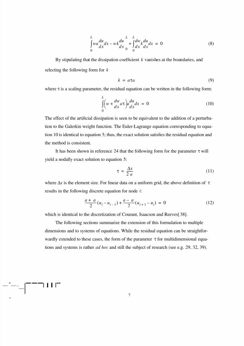
(8)
By stipulating that the dissipation coefficient vanishes at the boundaries, and
selecting the following form for
(9)
where τ is a scaling parameter, the residual equation can be written in the following form:
(10)
The effect of the artificial dissipation is seen to be equivalent to the addition of a perturba-tion to the Galerkin weight function. The Euler-Lagrange equation corresponding to equa-
tion 10 is identical to equation 5; thus, the exact solution satisfies the residual equation and
the method is consistent.
It has been shown in reference 24 that the following form for the parameter τ will
yield a nodally exact solution to equation 5:
(11)
where ∆ x is the element size. For linear data on a uniform grid, the above definition of τ
results in the following discrete equation for node i:
(12)
which is identical to the discretization of Courant, Isaacson and Reeves[38].
The following sections summarize the extension of this formulation to multiple
dimensions and to systems of equations. While the residual equation can be straightfor-
wardly extended to these cases, the form of the parameter τ for multidimensional equa-
tions and systems is rather ad hoc and still the subject of research (see e.g. 29, 32, 39).
wa xd
du xd wk
xd
du
0
L
– xd
dwk
xd
du xd
0
L
∫ +
0
L
∫ 0=
k
k
k aτa=
w xd
dwaτ+
a xd
du xd
0
L
∫ 0=
τ x∆2 a---------=
a a+
2--------------- ui ui 1––( ) a a–
2-------------- ui 1+ ui–( )+ 0=
8/8/2019 A Higher Order Accurate Finite Element Method for Viscous Compressible Flows
http://slidepdf.com/reader/full/a-higher-order-accurate-finite-element-method-for-viscous-compressible-flows 16/86
8
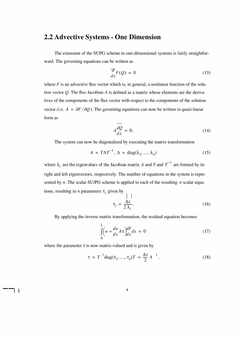
2.2 Advective Systems - One Dimension
The extension of the SUPG scheme to one-dimensional systems is fairly straightfor-
ward. The governing equations can be written as
(13)
where F is an advective flux vector which is, in general, a nonlinear function of the solu-
tion vector Q. The flux Jacobian A is defined as a matrix whose elements are the deriva-
tives of the components of the flux vector with respect to the components of the solution
vector (i.e. ). The governing equations can now be written in quasi-linear
form as
. (14)
The system can now be diagonalized by executing the matrix transformation
, (15)
where are the eigenvalues of the Jacobian matrix A and T and are formed by its
right and left eigenvectors, respectively. The number of equations in the system is repre-sented by n. The scalar SU/PG scheme is applied to each of the resulting n scalar equa-
tions, resulting in n parameters given by
. (16)
By applying the inverse matrix transformation, the residual equation becomes
(17)
where the parameter τ is now matrix-valued and is given by
. (18)
xd
d F Q( ) 0=
A F ∂ Q∂ ⁄ =
A xd
dQ0=
A T ΛT 1–
= Λ diag λ1 … λn, ,( )=
λi T 1–
τi
τi
x∆2 λi
-----------=
w
xd
dw Aτ+
xd
dF xd
0
L
∫ 0=
τ T 1–diag τ1 … τn, ,( )T
x∆2
------ A1–
= =
8/8/2019 A Higher Order Accurate Finite Element Method for Viscous Compressible Flows
http://slidepdf.com/reader/full/a-higher-order-accurate-finite-element-method-for-viscous-compressible-flows 17/86
9
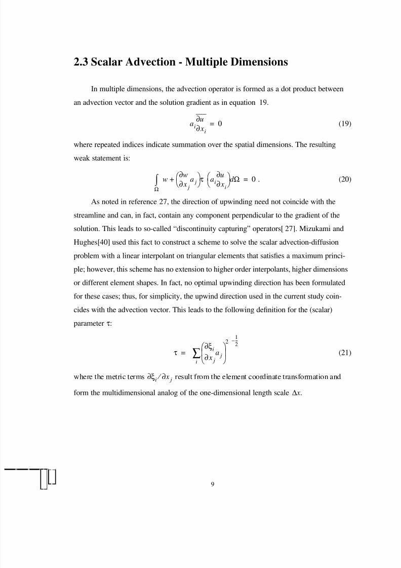
2.3 Scalar Advection - Multiple Dimensions
In multiple dimensions, the advection operator is formed as a dot product between
an advection vector and the solution gradient as in equation 19.
(19)
where repeated indices indicate summation over the spatial dimensions. The resulting
weak statement is:
. (20)
As noted in reference 27, the direction of upwinding need not coincide with the
streamline and can, in fact, contain any component perpendicular to the gradient of the
solution. This leads to so-called “discontinuity capturing” operators[27]. Mizukami and
Hughes[40] used this fact to construct a scheme to solve the scalar advection-diffusion
problem with a linear interpolant on triangular elements that satisfies a maximum princi-
ple; however, this scheme has no extension to higher order interpolants, higher dimensions
or different element shapes. In fact, no optimal upwinding direction has been formulated
for these cases; thus, for simplicity, the upwind direction used in the current study coin-
cides with the advection vector. This leads to the following definition for the (scalar)
parameter τ:
(21)
where the metric terms result from the element coordinate transformation and
form the multidimensional analog of the one-dimensional length scale ∆ x.
ai xi∂∂u
0=
w x j∂
∂wa j
τ+ ai xi∂∂u
Ωd
Ω∫ 0=
τ x j∂
∂ξia j
2
i∑
1
2---–
=
ξi∂ x j∂ ⁄
8/8/2019 A Higher Order Accurate Finite Element Method for Viscous Compressible Flows
http://slidepdf.com/reader/full/a-higher-order-accurate-finite-element-method-for-viscous-compressible-flows 18/86
10
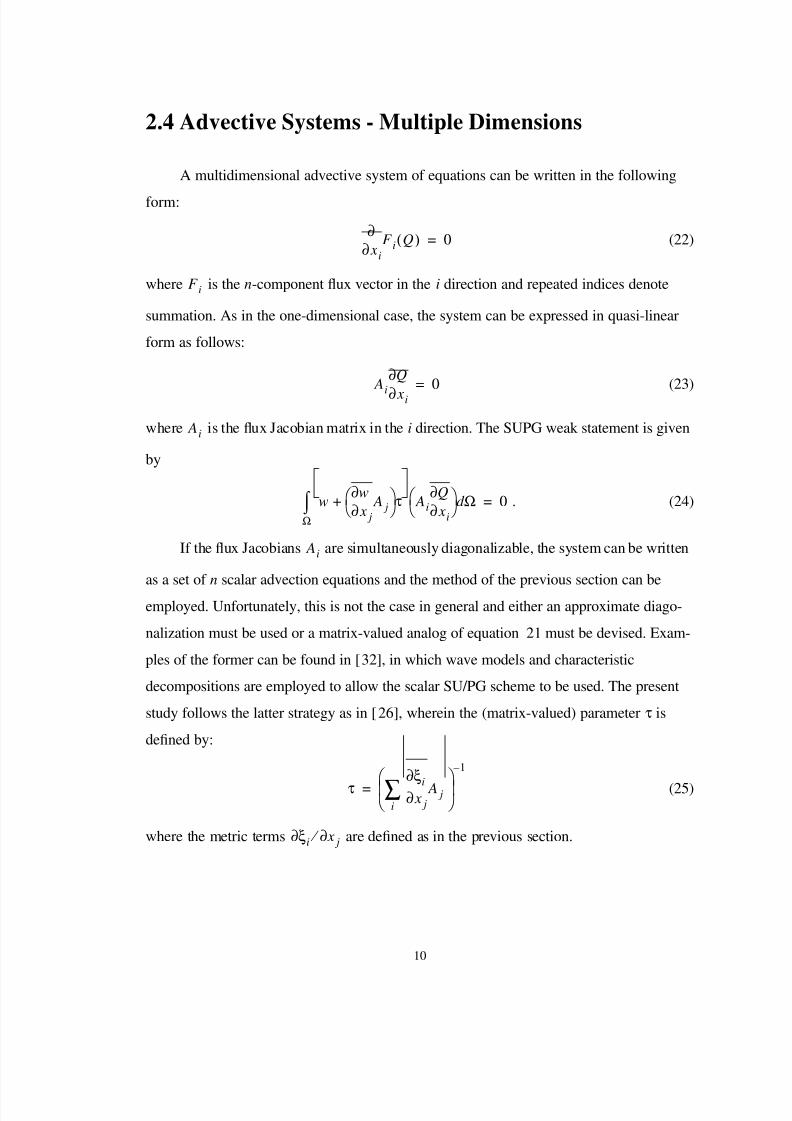
2.4 Advective Systems - Multiple Dimensions
A multidimensional advective system of equations can be written in the following
form:
(22)
where is the n-component flux vector in the i direction and repeated indices denote
summation. As in the one-dimensional case, the system can be expressed in quasi-linear
form as follows:
(23)
where is the flux Jacobian matrix in the i direction. The SUPG weak statement is given
by
. (24)
If the flux Jacobians are simultaneously diagonalizable, the system can be written
as a set of n scalar advection equations and the method of the previous section can be
employed. Unfortunately, this is not the case in general and either an approximate diago-
nalization must be used or a matrix-valued analog of equation 21 must be devised. Exam-
ples of the former can be found in [32], in which wave models and characteristic
decompositions are employed to allow the scalar SU/PG scheme to be used. The present
study follows the latter strategy as in [26], wherein the (matrix-valued) parameter τ is
defined by:
(25)
where the metric terms are defined as in the previous section.
xi∂∂
F i Q( ) 0=
F i
Ai xi∂∂Q
0=
Ai
w x j∂
∂w A j
τ+ Ai xi∂∂Q
Ωd
Ω∫ 0=
Ai
τ x j∂
∂ξi A j
i∑
1–
=
ξi∂ x j∂ ⁄

8/8/2019 A Higher Order Accurate Finite Element Method for Viscous Compressible Flows
http://slidepdf.com/reader/full/a-higher-order-accurate-finite-element-method-for-viscous-compressible-flows 19/86
11
Chapter 3
Quasi-One-Dimensional Euler Equations
3.1 Governing Equations
The equations solved are the one-dimensional Euler equations in conservation form
with a source term to account for the variation of cross-sectional area. The equations can
be written as
(26)
where
, , (27)
where ρ is the density, u is the speed, p is the pressure, e is the internal energy per unit
mass, h is the enthalpy per unit mass, A is the cross-sectional area, and a subscript “0”
indicates a stagnation condition.
The pressure is related to density and energy via the ideal-gas equation of state given
by
(28)
where γ is the ratio of specific heats.
The equations are solved in nondimensional form by defining the following nondi-
x∂∂
F Q( ) S Q( )=
Q
ρρu
ρe0
= F
ρu
ρu2
p+
ρuh0
= S1
A---
xd
dAρu
ρu2
ρuh0
–=
p γ 1–( )ρe=

8/8/2019 A Higher Order Accurate Finite Element Method for Viscous Compressible Flows
http://slidepdf.com/reader/full/a-higher-order-accurate-finite-element-method-for-viscous-compressible-flows 20/86

8/8/2019 A Higher Order Accurate Finite Element Method for Viscous Compressible Flows
http://slidepdf.com/reader/full/a-higher-order-accurate-finite-element-method-for-viscous-compressible-flows 21/86
13
. (34)
After integration of the Galerkin part of the flux term by parts, this statement becomes
(35)
At the upstream boundary, total pressure and total temperature are specified while
density is evaluated just inside the boundary. At the downstream boundary, density and
velocity are evaluated on the interior while a back pressure is prescribed. These boundary
conditions are enforced weakly via the boundary flux term of equation 35.
3.3 Solution Methodology
The physical domain is divided uniformly into elements of length ∆ x.
This results in a constant transformation to a local element coordinate system in which the
differential and the derivative are given by:
, (36)
where ξ is the barycentric coordinate in an element. The flow variables Q are approxi-
mated by a Bezier curve over each element given by:
(37)
where the are the discrete control points and the are the univariate Bernstein poly-
nomials of degree n given by
. (38)
After writing the global integrals in equation 35 as a sum of element integrals and
w xd
dw Aτ+
xd
dF S–
xd
x0
x L
∫ 0=
wF x0
x L
xd
dwF xd
x0
x L
∫ – wS xd
x0
x L
∫ – xd
dw Aτ
xd
dF S–
xd
x0
x L
∫ + 0=
x x0 x L,[ ]∈
xd d xd ⁄
xd x ξd ∆= xd d 1 x∆------ ξd d =
Q ξ( ) Qi Bi
n ξ( )i 0=
n
∑=
Qi Bi
n
Bi
n ξ( ) n!
i! n i–( )!--------------------- ξi
1 ξ–( )n i–=

8/8/2019 A Higher Order Accurate Finite Element Method for Viscous Compressible Flows
http://slidepdf.com/reader/full/a-higher-order-accurate-finite-element-method-for-viscous-compressible-flows 22/86
14
substituting the above data representation and coordinate transformation, the weak state-
ment now becomes
(39)
The element integrals appearing in equation 39 are evaluated numerically via Gaussian
quadrature given by
(40)
where the weights and ordinates are given in [12].
To obtain the solution Q, Newton’s method is applied to equation 39. First, the weak
statement is linearized about an initial solution to obtain a linear system of equations
in the following form:
(41)
where is the j-th weak statement evaluated on the initial solution and is the
update to the control point .
The term is the Jacobian matrix of the system and is evaluated approxi-
mately by the following equation:
. (42)
Note that this Jacobian is approximate because the dependencies of the flux Jacobian A
and the Jacobian of the source term ( ) on the solution variables Q are not included.
Hence the resulting iterate will not recover the quadratic convergence of Newton’s
B jF 0
L
ξd
dB j
F ξd 0
1
∫ – B jS x ξd ∆0
1
∫ – xd
dB j
Asgn1
x∆------ ξd
dF S– ξd
0
1
∫ +Ωe∑+ 0=
f ξ( ) ξd
0
1
∫ wi f ξi( )i 1=
N
∑≈
wi ξi
Qn
Qi∂∂ R j ∆Qi R j+ 0=
R j Qn ∆Qi
Qi
n
R j∂ Qi∂ ⁄
Qi∂∂ R j
wAB j0
L
ξd
dB j AB i ξd
0
1
∫ – B j Q∂∂S
Bi x ξd ∆0
1
∫ –
xd
dB j Asgn
1
x∆
------ A
ξ∂
∂ Bi
Q∂
∂S Bi–
ξd
0
1
∫
+Ωe
∑+≈
S∂ Q∂ ⁄
8/8/2019 A Higher Order Accurate Finite Element Method for Viscous Compressible Flows
http://slidepdf.com/reader/full/a-higher-order-accurate-finite-element-method-for-viscous-compressible-flows 23/86
15
method.
Because neighboring elements are coupled only through their shared interface, the
linear system represented by equation 41 is a block banded system with a maximum band-
width of 3x3 blocks. This system is solved directly using banded Gaussian elimi-
nation to compute the solution updates . This process is repeated until the nonlinear
system represented by equation 39 is satisfied to a given tolerance.
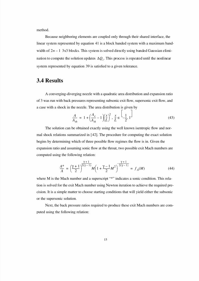
3.4 Results
A converging-diverging nozzle with a quadratic area distribution and expansion ratio
of 3 was run with back pressures representing subsonic exit flow, supersonic exit flow, and
a case with a shock in the nozzle. The area distribution is given by
, (43)
The solution can be obtained exactly using the well known isentropic flow and nor-
mal shock relations summarized in [42]. The procedure for computing the exact solution
begins by determining which of three possible flow regimes the flow is in. Given the
expansion ratio and assuming sonic flow at the throat, two possible exit Mach numbers are
computed using the following relation:
(44)
where M is the Mach number and a superscript “*” indicates a sonic condition. This rela-
tion is solved for the exit Mach number using Newton iteration to achieve the required pre-
cision. It is a simple matter to choose starting conditions that will yield either the subsonic
or the supersonic solution.
Next, the back pressure ratios required to produce these exit Mach numbers are com-
puted using the following relation:
2n 1–
∆Qi
A
Ath
------- 1 Ae
Ath
------- 1– x
L---
2+=x
L---
1
2--- 1,–∈
A∗ A------
γ 1+
2------------
γ 1+
2 γ 1–( )--------------------
M 1γ 1–
2----------- M
2+
γ 1+
2 γ 1–( )--------------------–
f A M ( )= =
8/8/2019 A Higher Order Accurate Finite Element Method for Viscous Compressible Flows
http://slidepdf.com/reader/full/a-higher-order-accurate-finite-element-method-for-viscous-compressible-flows 24/86
16
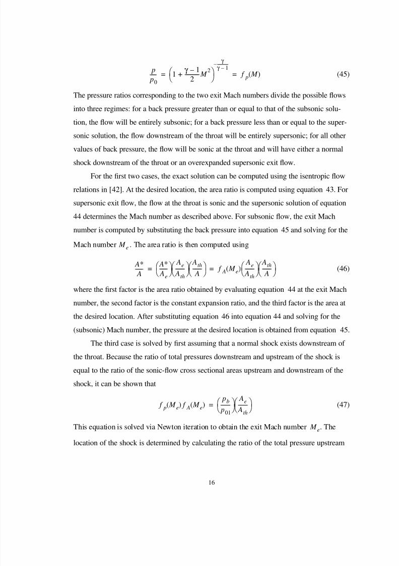
(45)
The pressure ratios corresponding to the two exit Mach numbers divide the possible flowsinto three regimes: for a back pressure greater than or equal to that of the subsonic solu-
tion, the flow will be entirely subsonic; for a back pressure less than or equal to the super-
sonic solution, the flow downstream of the throat will be entirely supersonic; for all other
values of back pressure, the flow will be sonic at the throat and will have either a normal
shock downstream of the throat or an overexpanded supersonic exit flow.
For the first two cases, the exact solution can be computed using the isentropic flow
relations in [42]. At the desired location, the area ratio is computed using equation 43. For
supersonic exit flow, the flow at the throat is sonic and the supersonic solution of equation
44 determines the Mach number as described above. For subsonic flow, the exit Mach
number is computed by substituting the back pressure into equation 45 and solving for the
Mach number . The area ratio is then computed using
(46)
where the first factor is the area ratio obtained by evaluating equation 44 at the exit Mach
number, the second factor is the constant expansion ratio, and the third factor is the area at
the desired location. After substituting equation 46 into equation 44 and solving for the
(subsonic) Mach number, the pressure at the desired location is obtained from equation 45.
The third case is solved by first assuming that a normal shock exists downstream of
the throat. Because the ratio of total pressures downstream and upstream of the shock is
equal to the ratio of the sonic-flow cross sectional areas upstream and downstream of the
shock, it can be shown that
(47)
This equation is solved via Newton iteration to obtain the exit Mach number . The
location of the shock is determined by calculating the ratio of the total pressure upstream
p
p0
----- 1γ 1–
2----------- M
2+
γ
γ 1–-----------–
f p M ( )= =
M e
A∗ A------
A∗ Ae
------ Ae
Ath
------- Ath
A-------
f A M e( ) Ae
Ath
------- Ath
A-------
= =
f p M e( ) f A M e( ) pb
p01
-------- Ae
Ath
------- =
M e

8/8/2019 A Higher Order Accurate Finite Element Method for Viscous Compressible Flows
http://slidepdf.com/reader/full/a-higher-order-accurate-finite-element-method-for-viscous-compressible-flows 25/86
17
and downstream of the shock:
(48)
This ratio is also defined by the normal shock relation
(49)
which is solved via Newton iteration for the upstream Mach number at the shock, .
Equation 44 now yields the area ratio at the shock. If this area ratio is less than the expan-
sion ratio, equation 43 is used to compute the location of the shock, otherwise, the shock is
downstream of the exit.
The solution upstream of the shock is now computed as previously described by
solving equation 44 for the (supersonic) Mach number. Downstream of the shock, the area
ratio must be adjusted to account for losses through the shock as follows:
(50)
The subsonic solution of equation 44 gives the Mach number at the desired location. The
calculation of the pressure must also account for losses across the shock as follows:
(51)
Three different values of back pressure were used representing the three flow
regimes described previously. The first case, at a back pressure ratio of 0.98, represents a
purely subsonic unchoked flow. The second case, at a back pressure of 0.28, represents
purely supersonic flow downstream of the throat. The final case, at a back pressure of 0.88,
represents a flow with a shock between the throat and exit. Several different orders of
accuracy were used and the integrated error in the pressure distribution defined by
p02
p01
-------- p02
pb
-------- pb
p01
-------- f p M e( )
pb
p01
-------- = =
p02
p01
--------γ 1+
2γ M 2 γ 1–( )–
-------------------------------------
1
γ 1–-----------
γ 1+( ) M 2
γ 1–( ) M 2
2+----------------------------------
γ γ 1–-----------
g p M ( )= =
M s
A∗ A------
A2∗
A1∗
--------- A1
∗
A---------
g p M s( ) Ath
A-------
= =
p
p01
-------- p02
p01
-------- p
p02
-------- g p M s( ) f p M ( )= =
L2

8/8/2019 A Higher Order Accurate Finite Element Method for Viscous Compressible Flows
http://slidepdf.com/reader/full/a-higher-order-accurate-finite-element-method-for-viscous-compressible-flows 26/86
18
(52)
where is the exact solution, was calculated for several different grid sizes.
The first case is a purely subsonic flow resulting from a back pressure ratio of 0.98.
Figure 1 shows the integrated norm of the pressure error versus the number of degrees of
freedom in the problem. Design accuracy was verified up to 9th order (beyond this point
64-bit floating point numbers lack sufficient precision to resolve the spatial convergence
rate of the scheme). Note that up to about degree 5 (order of accuracy 6) there are signifi-
cant gains to increasing the order of accuracy as the 6th order result can be up to 5 orders
of magnitude more accurate than the 2nd order result. Also note that for linear data thescheme is superconvergent and results in a 3rd order solution.
Figure 2 shows pressure error for a case with supersonic exit flow. Note that for lin-
ear data the scheme is no longer superconvergent, but otherwise the same trends in accu-
racy are observed up to fifth order.
For the case of a normal shock in the nozzle, all linear schemes are at best first order
accurate globally. Figure 3 shows the distribution of pressure error for a 4th order solution.
The parameter J is the number of elements. Note that while the upstream flow is achieving
design accuracy, the solution is at best first order not only at the shock but also down-
stream of the shock. This problem was discovered by Casper and Carpenter[41] and is also
observed in these results.
These results verify that the SU/PG scheme as formulated for linear solution data
(i.e. 2nd order schemes) can be used without modification to achieve higher order accu-
racy for smooth flows.
L2
p x( ) p x( )–[ ]2 xd
x0
x L
∫ =
p

8/8/2019 A Higher Order Accurate Finite Element Method for Viscous Compressible Flows
http://slidepdf.com/reader/full/a-higher-order-accurate-finite-element-method-for-viscous-compressible-flows 27/86
19
Figure 1. Pressure error for converging-diverging nozzle with purely subsonic flow.

8/8/2019 A Higher Order Accurate Finite Element Method for Viscous Compressible Flows
http://slidepdf.com/reader/full/a-higher-order-accurate-finite-element-method-for-viscous-compressible-flows 28/86
20
Figure 2. Pressure error for converging-diverging nozzle with supersonic exit flow.

8/8/2019 A Higher Order Accurate Finite Element Method for Viscous Compressible Flows
http://slidepdf.com/reader/full/a-higher-order-accurate-finite-element-method-for-viscous-compressible-flows 29/86
21
Figure 3. Pressure error for converging-diverging nozzle flow with a standing shock.
8/8/2019 A Higher Order Accurate Finite Element Method for Viscous Compressible Flows
http://slidepdf.com/reader/full/a-higher-order-accurate-finite-element-method-for-viscous-compressible-flows 30/86
22
Chapter 4
Two-Dimensional Navier-Stokes Equa-
tions
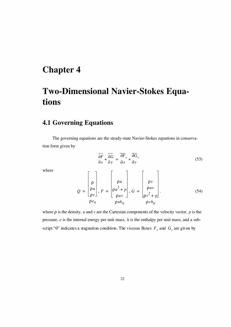
4.1 Governing Equations
The governing equations are the steady-state Navier-Stokes equations in conserva-
tion form given by
(53)
where
, , . (54)
where ρ is the density, u and v are the Cartesian components of the velocity vector, p is the
pressure, e is the internal energy per unit mass, h is the enthalpy per unit mass, and a sub-
script “0” indicates a stagnation condition. The viscous fluxes and are given by
x∂∂F
y∂∂G
+ x∂
∂F v
y∂∂Gv
+=
Q
ρρu
ρv
ρe0
= F
ρu
ρu2
p+
ρuv
ρuh0
= G
ρv
ρuv
ρv2
p+
ρvh0
=
F v Gv

8/8/2019 A Higher Order Accurate Finite Element Method for Viscous Compressible Flows
http://slidepdf.com/reader/full/a-higher-order-accurate-finite-element-method-for-viscous-compressible-flows 31/86
23
, (55)
where the viscous stresses , , and are evaluated for a Newtonian fluid under the
bulk viscosity assumption.
, , (56)
where µ is the molecular viscosity. The heat flux components and are given by Fou-
rier’s law:
, (57)
where k is the Fourier heat transfer coefficient and T is the static temperature.
The pressure is related to density and energy via the ideal-gas equation of state given
by
(58)
while the following power law valid for air at temperatures from 300˚R to 900˚R[42] isused to relate viscosity to temperature
(59)
where the subscript r denotes a reference condition.
The equations are solved in nondimensional form by defining the following nondi-
mensional quantities:
, , , , , , , ,
, , (60)
F v
0
τ xx
τ xy
uτ xx vτ xy q x–+
= Gv
0
τ xy
τ yy
uτ xy vτ yy q y–+
=
τ xx τ xy τ yy
τ xx µ 4
3---
x∂∂u 2
3---
y∂∂v
– = τ xy µ
y∂∂u
x∂∂v
+ = τ yy µ 4
3---
y∂∂v 2
3---
x∂∂u
– =
q x q y
q x k x∂
∂T –= q y k
y∂∂T
–=
p γ 1–( )ρe=
µµr
-----T
T r
----- 0.76
=
x∗x
L---= y∗y
L---= ρ∗ ρρ∞------= u∗
u
c∞------= v∗
v
c∞------= p∗
p
ρ∞c∞2-------------= T ∗
RT
c∞2-------= e∗
e
c∞2------=
h∗ h
c∞2
------= µ∗ µµ∞------= k ∗ k
k ∞------=
8/8/2019 A Higher Order Accurate Finite Element Method for Viscous Compressible Flows
http://slidepdf.com/reader/full/a-higher-order-accurate-finite-element-method-for-viscous-compressible-flows 32/86
24
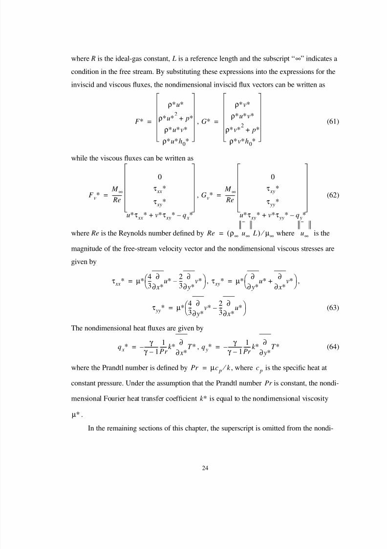
where R is the ideal-gas constant, L is a reference length and the subscript “∞” indicates a
condition in the free stream. By substituting these expressions into the expressions for the
inviscid and viscous fluxes, the nondimensional inviscid flux vectors can be written as
, (61)
while the viscous fluxes can be written as
, (62)
where Re is the Reynolds number defined by where is the
magnitude of the free-stream velocity vector and the nondimensional viscous stresses are
given by
, ,
(63)
The nondimensional heat fluxes are given by
, (64)
where the Prandtl number is defined by , where is the specific heat at
constant pressure. Under the assumption that the Prandtl number Pr is constant, the nondi-
mensional Fourier heat transfer coefficient is equal to the nondimensional viscosity
.
In the remaining sections of this chapter, the superscript is omitted from the nondi-
F ∗
ρ∗u∗
ρ∗u∗2 p∗+
ρ∗u∗v∗
ρ∗u∗h0∗
= G∗
ρ∗v∗
ρ∗u∗v∗
ρ∗v∗2 p∗+
ρ∗v∗h0∗
=
F v∗M ∞ Re--------
0
τ xx∗τ xy
∗
u∗τ xx∗ v∗τ xy
∗ q x∗–+
= Gv∗ M ∞
Re--------
0
τ xy∗τ yy
∗
u∗τ xy∗ v∗τ yy
∗ q y∗–+
=
Re ρ∞ u∞ L( ) µ∞ ⁄ = u∞
τ xx
∗µ
∗ 4
3---
x∗∂
∂u∗ 2
3---
y∗∂
∂v∗–
=
τ xy
∗µ
∗ y∗∂
∂u∗
x∗∂
∂v∗+
=
τ yy∗ µ∗ 4
3---
y∗∂∂
v∗ 2
3---
x∗∂∂
u∗– =
q x∗ γ
γ 1–-----------
1
Pr ------k ∗
x∗∂∂
T ∗–= q y∗ γ
γ 1–-----------
1
Pr ------k ∗
y∗∂∂
T ∗–=
Pr µc p k ⁄ = c p
k ∗
µ∗
8/8/2019 A Higher Order Accurate Finite Element Method for Viscous Compressible Flows
http://slidepdf.com/reader/full/a-higher-order-accurate-finite-element-method-for-viscous-compressible-flows 33/86
25
mensional quantities for the sake of clarity.
4.2 Finite Element Formulation
The Petrov-Galerkin weak statement of equation 53 is given by:
(65)
where the matrix τ is defined as in chapter 2. By integrating the Galerkin terms by parts,
the above weak statement becomes:
(66)
where and are the Cartesian components of the boundary surface unit normal vector
. The fluxes in the boundary integrals are evaluated based on the boundary conditions as
described in the following paragraphs.
The inviscid flux on the boundary can be written as:
(67)
On both inviscid and no-slip surfaces, the normal velocity vanishes, resulting in the
following boundary flux:
w x∂
∂w A
y∂∂w
B+ τ+
x∂∂F
y∂∂G M ∞
Re--------
x∂∂F v
y∂∂Gv
+ –+ Ωd
Ω∫ 0=
w Fn x Gn y+( ) Γ d
Γ ∫
M ∞ Re-------- w F vn x Gvn y+( ) Γ d
Γ ∫ –
x∂∂w
F y∂
∂wG+
Ωd
Ω∫ –
M ∞
Re--------
x∂∂w
F v y∂∂w
Gv+ Ωd
Ω∫ x∂
∂w A
y∂∂w
B+ τ
x∂∂F
y∂∂G M ∞
Re--------
x∂∂F v
y∂∂Gv
+ –+ Ωd
Ω∫
+
+ 0=
n x n y
n
Fn x Gn y+
ρun x ρvn y+
ρu2
p+( )n x ρuv n y+
ρuv n x ρv2
p+( )n y+
ρuhn x ρvh n y+
ρu n⋅ρuu n pn x+⋅
ρvu n pn y+⋅
ρhu n⋅
= =
u n⋅
8/8/2019 A Higher Order Accurate Finite Element Method for Viscous Compressible Flows
http://slidepdf.com/reader/full/a-higher-order-accurate-finite-element-method-for-viscous-compressible-flows 34/86
26
(68)
where the pressure p is evaluated just inside the boundary. For subsonic flow across an
inflow/outflow boundary, the inviscid flux is evaluated by computing the normal velocity
and speed of sound from two locally one-dimensional Riemann invariants given by
(69)
The quantity is evaluated using free-stream conditions while is evaluated based on
values just inside the domain. The normal velocity and speed of sound on the boundary are
then given by
, (70)
The velocity components on the boundary are found by decomposing the normal velocity
(given by equation 70) and the tangential velocity into components resulting in the follow-
ing expressions:
, (71)
where the subscript r denotes a reference condition in the free stream for flow into the
domain and just inside the boundary for flow out of the domain. Similarly, entropy on the
boundary is calculated from free-stream quantities for flow into the domain and from inte-
rior values for outflow. The density on the boundary is then calculated as
(72)
For supersonic inflow and outflow, the boundary flux vector is calculated entirely from
quantities in the free stream and just inside the boundary, respectively.
The viscous flux vector on the boundary can be written as
Fn x Gn y+
0
pn x
pn y
0
=
R±
u n2c
γ 1–-----------±⋅=
R–
R+
u n⋅( )b
1
2--- R
+ R
–+( )= cb
γ 1–
4----------- R
+ R
––( )=
ub ur n x u n⋅( )b u n⋅( )r –[ ]+= vb vr n y u n⋅( )b u n⋅( )r –[ ]+=
ρb
cb
2
γ Sb
--------
1
γ 1–-----------
=
8/8/2019 A Higher Order Accurate Finite Element Method for Viscous Compressible Flows
http://slidepdf.com/reader/full/a-higher-order-accurate-finite-element-method-for-viscous-compressible-flows 35/86
27
(73)
On inviscid and inflow/outflow boundaries, the viscous flux is assumed to be zero. On no-
slip surfaces the condition is strongly enforced, replacing the momentum
equations on those surfaces. As a result, the second and third elements of the boundary
flux vector are irrelevant, and the fourth reduces to . An adiabatic wall is assumed,
so this term also vanishes. Thus, the integral of the viscous boundary flux vanishes on all
boundaries.
4.3 Solution Methodology
4.3.1 Discretization
The physical domain Ω is divided into a set of nonoverlapping triangular elements
such that the entire domain is represented. The solution data Q are represented by tri-
angular Bezier patches in each element defined by
(74)
where ξ and η are the local barycentric coordinates of the element and the are the
bivariate Bernstein polynomials of degree n given by
. (75)
To accommodate curved boundaries, the coordinates of each triangular element are
also represented by triangular Bezier patches of degree n. This results in a nonlinear coor-
dinate transformation from the physical space to the element parameter space. Derivatives
in physical space ( x, y) are transformed to element parameter space (ξ, η) by
F vn x Gvn y+
0
τ xx n x τ xy n y+
τ xy n x τ yy n y+
uτ xx vτ xy+( )n x uτ xy vτ yy+( )n y
k T ∇ n⋅+ +
=
u v 0= =
k T ∇ n⋅
Ωe
Q ξ η,( ) Qij Bij
n ξ η,( ) j 0=
n i–
∑i 0=
n
∑=
Bij
n
Bij
n ξ η,( ) n!
i! j! n i– j–( )!----------------------------------ξiη j
1 ξ– η–( )n i– j–=

8/8/2019 A Higher Order Accurate Finite Element Method for Viscous Compressible Flows
http://slidepdf.com/reader/full/a-higher-order-accurate-finite-element-method-for-viscous-compressible-flows 36/86
28
, . (76)
The metric terms appearing in equation 76 can be expressed in terms of the deriva-
tives of the element coordinates as
, , , (77)
where J is the Jacobian of the element coordinate transformation defined by
. (78)
Finally, the volume differential is scaled by the Jacobian J as follows:
. (79)
Continuity of the solution across element interfaces is enforced by sharing control
points along the interfaces as illustrated in figure 4a. The indexing in equation 74 is
converted to a single index as shown in figure 4b by the following function:
(80)
The boundary Γ of the domain Ω is divided into a finite number of line elements ,
each of which corresponds to the edge of a triangular element adjoining the boundary as
shown in figure 5. The coordinates and data on each of these elements is represented by a
Bezier curve of degree n as described in the previous chapter. Integrals over the boundary
Γ can now be written as sums of integrals over individual boundary elements. These ele-
ment integrals are transformed into integrals over the local element parameter space.
The polynomial expression of the boundary element coordinates gives rise to a con-
tinuously varying unit normal along curved elements. The components of the element nor-
mal vector are given by
, . (81)
Boundary element integrals are transformed according to
x∂∂
x∂∂ξ
ξ∂∂
x∂∂η
η∂∂
+= y∂∂
y∂∂ξ
ξ∂∂
y∂∂η
η∂∂
+=
x∂∂ξ 1
J ---
η∂∂ y
= y∂
∂ξ 1
J ---–
η∂∂ x
= x∂
∂η 1
J ---–
ξ∂∂ y
= y∂
∂η 1
J ---
ξ∂∂ x
=
J ξ∂
∂ xη∂
∂ yη∂
∂ xξ∂
∂ y–=
Ωed
Ωed J ξ ηd d =
i j,( )
inode j 2n j– 3+( ) 2 ⁄ i+=
Γ e
n x ξ∂∂ y
= n y ξ∂∂ x
–=
8/8/2019 A Higher Order Accurate Finite Element Method for Viscous Compressible Flows
http://slidepdf.com/reader/full/a-higher-order-accurate-finite-element-method-for-viscous-compressible-flows 37/86
29
(82)
where
. (83)
Upon substitution of the foregoing domain and boundary transformations, the weak
statement (equation 66) can now be written as
(84)
where
, (85)
are the transformed inviscid flux vectors and and are the corresponding flux Jacobi-
ans. The transformed viscous fluxes and are similarly defined. Note that the contri-
bution of the viscous terms to the Petrov-Galerkin part of the weak statement has been
neglected. These terms involve derivatives of the metric terms and are therefore difficult to
compute. Reference 43 presents a local reconstruction technique to represent this contri-
bution that may be incorporated in future work. As will be seen in the results, this omis-
sion has no impact on the order properties of the scheme.
The integrals appearing in equation 84 are evaluated numerically using the Gaussian
quadrature rules of [44] for triangular elements and [12] for the line elements on the
boundary. Finite element theory dictates that numerical quadrature must integrate polyno-
f x y,( ) Γ ed
Γ e∫ f x ξ( ) y ξ( ),[ ]s ξd
0
1
∫ =
sξ∂
∂ x
2
ξ∂∂ y
2
+=
Bij
nFn x Gn y+( )s ξd
0
1
∫ M ∞ Re-------- Bij
nF vn x Gvn y+( )s ξd
0
1
∫ –Γ e∑
ξ∂∂ Bij
n
F ˜η∂
∂ Bij
n
G+
J ξ ηd d
0
1 η–
∫ 0
1
∫ – M ∞ Re--------
ξ∂∂ Bij
n
F ˜v η∂
∂ Bij
n
Gv+
J ξ ηd d
0
1 η–
∫ 0
1
∫
ξ∂∂ Bij
n
Aη∂
∂ Bij
n
B+
τ Aξ∂
∂Q B
η∂∂Q
+ J ξ ηd d
0
1 η–
∫ 0
1
∫
+ +Ωe
∑
+
0=
F ˜
x∂∂ξ
F y∂∂ξ
G+= G˜
x∂∂η
F y∂∂η
G+=
A B
F ˜v Gv

8/8/2019 A Higher Order Accurate Finite Element Method for Viscous Compressible Flows
http://slidepdf.com/reader/full/a-higher-order-accurate-finite-element-method-for-viscous-compressible-flows 38/86
30
mials of degree exactly to preserve the convergence properties of the
scheme[12]. Here n is the degree of the interpolant and m is the highest order derivative
appearing in the integrand. This means that quadrature rules for triangular elements must
be exact to degree while boundary quadrature must be exact to degree . Gaus-
sian quadrature results in the minimum computational work for a given degree of accu-
racy, but availability of quadrature rules for triangular elements limits the scheme to fifth
order accuracy.
4.3.2 Solution Procedure
The solution Q is obtained using an approximate Newton method. First, the weak
statement (equation 84) is approximately linearized about an initial solution to give
(86)
where a pseudotime term has been added to improve diagonal dominance and allow more
robust convergence. The mass matrix is defined as
(87)
where is the element area. Note that this is an approximation of the true mass matrix,
but time accuracy is not at issue, and the approximation allows the integral to be evaluated
analytically and independent of the element shape - thus it can be precomputed and stored.
The system of linear equations represented by equation 86 is solved using the Gener-
alized Minimum Residual method (GMRES) described in [45], which computes the solu-
tion of a general linear system iteratively by projecting the residual onto vectors in the
Krylov subspace (An overview of Krylov subspace methods is given by Saad[46]). The
GMRES algorithm yields an exact solution if all the Krylov vectors are used; however, in
practice a subset of these vectors must be chosen to minimize storage requirements. Most
2 n m–( )
2 n 1–( ) 2n
Qn
M ij
t ∆--------
Qi∂∂ R j
+
∆Qi R j+ 0=
M ij
M ij Se Bkln Bqr
n ξ ηd d
0
1 η–
∫ 0
1
∫ Ωe
∑=
Se
8/8/2019 A Higher Order Accurate Finite Element Method for Viscous Compressible Flows
http://slidepdf.com/reader/full/a-higher-order-accurate-finite-element-method-for-viscous-compressible-flows 39/86
31
implementations of the algorithm allow the solution to be restarted when the allotted stor-
age for the Krylov vectors is exhausted. The implementation of the algorithm used in this
work allows specification of the number of Krylov vectors to store, the number of restarts
permitted, and a tolerance on the residual to use as a stopping criterion. Unless otherwise
noted, all the test cases presented in this chapter stored 20 Krylov vectors, allowed one
restart, and solved the system to a tolerance of 0.01.
The GMRES algorithm does not require explicit knowledge of the matrix of the lin-
ear system - only the product of the matrix with the vector is required. This allows
the product of the Jacobian and the solution update to be written as a finite-
difference expression as described in reference 47 and given by
(88)
where ε is a constant chosen such that the norm of is the square root of machine pre-
cision.
The performance of the GMRES algorithm depends, in general, on the use of a suit-
able preconditioner. The preconditioner should approximate the inverse of the matrix, but
must be simpler to solve. The simplest preconditioning is diagonal or Jacobi precondition-
ing, in which only diagonal terms of the matrix are retained and the resulting diagonal sys-
tem is solved. Other forms of preconditioning such as incomplete LU factorization[48] or
least-squares approximate inverse techniques[49, 50, 51] can improve convergence of the
GMRES algorithm at the expense of increased computational complexity and storage[48].
The preconditioning used in this work is a block-diagonal preconditioning in which
4x4 blocks are retained on the diagonal of the matrix. This preconditioning is easily solved
by inverting a 4x4 matrix for each degree of freedom. The block-diagonal matrix is repre-
sented by
(89)
where the diagonal block of the system Jacobian matrix is approximated by
∆Qi
R j∂ Qi∂ ⁄ ∆Qi
Qi∂∂ R j ∆Qi
R j Q ε∆Q+( ) R j Q( )–
ε------------------------------------------------------≈
ε∆Q
M kk
t ∆---------
Qk ∂∂ Rk
+
Rk ∂ Qk ∂ ⁄
8/8/2019 A Higher Order Accurate Finite Element Method for Viscous Compressible Flows
http://slidepdf.com/reader/full/a-higher-order-accurate-finite-element-method-for-viscous-compressible-flows 40/86
32
(90)
Note that the dependence of the flux Jacobians and of τ on the solution Q is neglected in
this approximation.
4.4 Inviscid Flow Results
4.4.1 Ringleb Flow
The first case presented is that of Ringleb’s flow, which is presented in detail by
Chiocchia[36]. This flow is an exact solution of the Euler equations for an ideal gas
obtained by using a hodograph transformation. The equations are transformed from the
Cartesian coordinate system to the hodograph plane where q is the velocity
magnitude and θ is the angle the velocity vector makes with a reference axis. The momen-
tum equations can be expressed in stream function form as
(91)
where ψ is the stream function defined such that the Cartesian velocity components are
given by
, (92)
where the subscript r indicates an arbitrary reference condition. This choice of stream
function identically satisfies the continuity equation.
Qk ∂∂ Rk
Bij
n An x Bn y+( ) Bij
ns ξd
0
1
∫ M ∞ Re-------- Bij
n Avn x Bvn y+( ) Bij
ns ξd
0
1
∫ –Γ e∑
ξ∂∂ Bij
n
Aη∂
∂ Bijn
B+
Bij
n J ξ ηd d
0
1 η–
∫ 0
1
∫ – M ∞ Re--------
ξ∂∂ Bij
n
Av η∂∂ Bij
n
Bv+
Bij
n J ξ ηd d
0
1 η–
∫ 0
1
∫
ξ∂∂ Bij
n
Aη∂
∂ Bij
n
B+
τ Aξ∂
∂ Bij
n
Bη∂
∂ Bij
n
+
J ξ ηd d
0
1 η–
∫ 0
1
∫
+ +Ωe
∑
+≈
x y,( ) q θ,( )
q2
q2
2
∂
∂ ψ q 1
q2
c2
-----+
q∂∂ψ
1q
2
c2
-----–
θ2
2
∂
∂ ψ + + 0=
uρr
ρ-----
y∂∂ψ
= vρr
ρ-----
x∂∂ψ
–=
8/8/2019 A Higher Order Accurate Finite Element Method for Viscous Compressible Flows
http://slidepdf.com/reader/full/a-higher-order-accurate-finite-element-method-for-viscous-compressible-flows 41/86
33
The particular solution representing Ringleb flow is given by
(93)
where the overbar indicates division by a reference quantity. The streamlines for this solu-
tion are given by
, (94)
where
(95)
The geometry is determined a posteriori by choosing two streamlines to serve as
solid walls along with lines of constant velocity as inflow and outflow boundaries. A typi-
cal geometry for this flow is shown in figure 6, where the solid walls are formed by
streamlines corresponding to and , and the outflow boundary is given by
.
In order to avoid the necessity of generating a high-order discretization of the curved
boundaries, triangular regions were selected from the traditional Ringleb flow domain.
One region lies entirely within the subsonic portion of the flow, while the other region is
within the supersonic region as illustrated in figure 6. Finite element meshes are generated
in each region by uniformly subdividing the region as shown in figure 7a. Additional
degrees of freedom required for the higher order interpolants are added via linear interpo-
lation of the mesh coordinates as illustrated in figure 7b. The exact solution was supplied
as a strongly enforced Dirichlet boundary condition.
Figure 8 shows the integrated norm of the error in the solution variables as a function
of the number of degrees of freedom. Note that design accuracy has been obtained up to
ψ 1
q--- θsin=
x1
2ρ------
1
q2
-----2
k 2
-----– J
2---+= y
1
k ρq--------- 1
q
k ---
2–±=
k 1 ψ ⁄ =
J 1
c
---1
3c3
--------1
5c5
--------1
2
---1 c+
1 c–
------------log–+ +=
c 1γ 1–
2-----------q
2–=
ρ c2 γ 1–( ) ⁄
=
k 0.8= k 1.6=
q 0.4=

8/8/2019 A Higher Order Accurate Finite Element Method for Viscous Compressible Flows
http://slidepdf.com/reader/full/a-higher-order-accurate-finite-element-method-for-viscous-compressible-flows 42/86
34
5th order. Similar behavior is noted in figure 9, which shows the integrated error norm for
the supersonic region.
4.4.2 Bump on a Wall
A simple case incorporating curved boundaries is shown in figure 10a. Four qua-
dratic segments form a bump on a wall whose height is 10% of its length. The segments
have continuous derivatives at their junction points. The mesh depicted in figure 10a is a
baseline mesh which was uniformly subdivided to control the number of unknowns in the
problem in a fashion similar to that used for Ringleb flow described in the previous sec-
tion. After subdividing and distributing additional degrees of freedom, the control points
on the lower wall were moved to match the Bezier representation of the geometry. An
example is given in figure 10b for a subdivision factor of 2 and cubic data.
Figure 11a shows the Mach number distribution along the lower wall for a free-
stream Mach number of 0.4. Note the considerable difference in the 2nd and 3rd order
solutions both at the peak and downstream to the outflow boundary. The SU/PG solutions
are also compared with results obtained from an implementation of a second order finite
volume scheme known as FUN2D[52]. Note that the finite volume results agree with the
second order SU/PG scheme at the peak, but the finite volume results are much more accu-
rate in the area of decelerating flow on the aft side of the bump. The second order SU/PG
scheme generates a significantly larger amount of entropy near the body than the finite
volume scheme as shown by the flow-field Mach number contours in figure 12. Note that
the contours for the finite volume solution smoothly approach the body while those for the
SU/PG solution show a significant jump in Mach number near the wall. This is an indica-
tion that while the SU/PG scheme achieves higher order accuracy, the relative error levels
may be improved by deriving an improved SU/PG formulation.
4.4.3 NACA 0012 Airfoil
Figure 13 shows a section of a mesh around a NACA 0012 airfoil obtained using the

8/8/2019 A Higher Order Accurate Finite Element Method for Viscous Compressible Flows
http://slidepdf.com/reader/full/a-higher-order-accurate-finite-element-method-for-viscous-compressible-flows 43/86
35
grid generation method of Marcum, et al.[53, 54]. The finest grid, depicted in the figure,
had 96 points distributed on the airfoil surface and 32 points distributed along a circular
outer boundary with a radius of 20 chord lengths. Two coarser meshes were generated by
selecting alternating points on the boundaries and retriangulating the volume.
The NACA 4-digit thickness profile[55] is given by
(96)
where t is the maximum thickness. By parametrizing x as , y can be written in
terms of ξ as
(97)
Thus the thickness distribution can be exactly represented by an 8th-order parametric Bez-
ier curve. To generate higher order finite element meshes, this defining curve was subdi-
vided to match the domain of each edge on the surface of an existing mesh and a least-
squares procedure was used to obtain the control points for the desired accuracy. The end-
points of each edge were forced to match the surface exactly.
The first case was run at a Mach number of 0.63 and an angle of attack of 2 degrees.
At these conditions, the flow is completely subsonic. Figure 14a shows the surface pres-sure distribution obtained using the SU/PG scheme for several orders of accuracy. Each
case has approximately the same number of degrees of freedom. Note the slight difference
in pressure between the 2nd and 3rd order solutions. A comparison of the SU/PG results
with results obtained from FUN2D are shown in figure 14b. The second order SU/PG
results are in close agreement with the finite volume results.
A second case at a Mach number of 0.8 and an angle of attack of 1.25 degrees was
run and surface pressure distributions obtained using FUN2D and the second and third
order SU/PG schemes is shown in figure 15. At these conditions, the flow is transonic and
shocks exist on both the upper and lower surfaces of the airfoil. Note that the two second
order schemes are in agreement and that the third order SU/PG scheme captures the upper
surface shock more sharply.
yt
0.2------- 0.29690 x 0.12600 x– 0.35160 x
2– 0.28430 x
30.10150 x
4–+( )±=
x ξ2=
yt
0.2
------- 0.29690ξ 0.12600ξ2– 0.35160ξ4
– 0.28430ξ60.10150ξ8
–+( )±=
8/8/2019 A Higher Order Accurate Finite Element Method for Viscous Compressible Flows
http://slidepdf.com/reader/full/a-higher-order-accurate-finite-element-method-for-viscous-compressible-flows 44/86
36
4.5 Laminar Viscous Flow Results
4.5.1 Couette Flow
To verify the formal accuracy of the scheme, a rotational Couette flow was com-
puted. The solution domain is depicted in figure 16a. Two concentric cylinders are in rela-
tive angular motion inducing fluid motion in the annular region. An analytic solution for
the angular velocity exists for incompressible flow and is given by:
(98)
where A and B are constants depending on the geometry and on the boundary conditions
and r is the distance from the common center of the cylinders. This solution also applies to
compressible flows as long as viscosity is constant. In a real flow, the temperature depen-
dence of viscosity couples the momentum and energy equations, but for the purpose of
establishing the accuracy of the scheme, this approximation will suffice.
Grids were generated by distributing Lagrange points for triangular elements along
lines of constant r and θ and then converting to the required Bezier description. A typical
grid for a second-order calculation is shown in figure 16b. Figure 17 shows the integrated
error in the circumferential velocity for a Couette flow where , ,
and . This particular choice of parameters results in an exact solution
for the circumferential velocity of
(99)
where the term dominates. The Mach number at the inner cylinder (0.2) and the Rey-
nolds number (500) were chosen to be relatively low to avoid violating the assumptions of
constant viscosity and laminar flow. The parameter n indicates the degree of the basis
functions. Design accuracy is confirmed up to fifth order. The case of quadratic data
appears to show superconvergence, but this result may be peculiar to this case (it is sus-
uθ Ar B
r ---+=
L2 r 1 1= r 2 4=
ω1 0.2= ω2 0=
uθ1
75------ r –
16
r ------+
=
1 r ⁄

8/8/2019 A Higher Order Accurate Finite Element Method for Viscous Compressible Flows
http://slidepdf.com/reader/full/a-higher-order-accurate-finite-element-method-for-viscous-compressible-flows 45/86
37
pected that the error may simply have no third-order components).
4.5.2 Flat Plate
The first case of practical interest is that of flow past a flat plate. Figure 18 shows the
solution domain and an initial discretization that forms the basis of all the following calcu-
lations. For each case, the finite-element grid is characterized by two parameters N and n.
The refinement parameter N indicates how many subdivisions of the baseline grid were
performed, while the parameter n is the degree of the interpolating polynomial. The num-
ber of degrees of freedom in the calculation is linearly related to the product of these two
parameters.
Since the Riemann-invariant boundary condition is strictly applicable only to invis-
cid flows, the abutment of a viscous surface and an outflow boundary results in significant
error over much of the plate; therefore a different boundary formulation is used. At the
inflow, total pressure, total temperature and normal velocity are specified while static pres-
sure is evaluated just inside the boundary. At the outflow, a back pressure is specified
while the energy and velocity are evaluated just inside the boundary.
Figure 19a shows skin friction distributions for several cases at a Mach number of
0.3 and a Reynolds number of 500. The well known incompressible solution of Bla-
sius[56] is shown for comparison. The flow conditions were chosen so as to compare
favorably with the Blasius solution while avoiding the ill conditioning of the equations at
very low Mach numbers[57]. Note that the higher order solutions are in closer agreement
to the Blasius solution than the second order solution. The results shown in figure 19b rep-
resent a uniform refinement of the cases in figure 19a. At this level of refinement, all the
schemes give visually similar distributions of the skin friction. Note that there is still a
small oscillation in the skin friction at the outflow for all the cases, probably due to thecombination of strong enforcement of the no-slip condition and weak enforcement of the
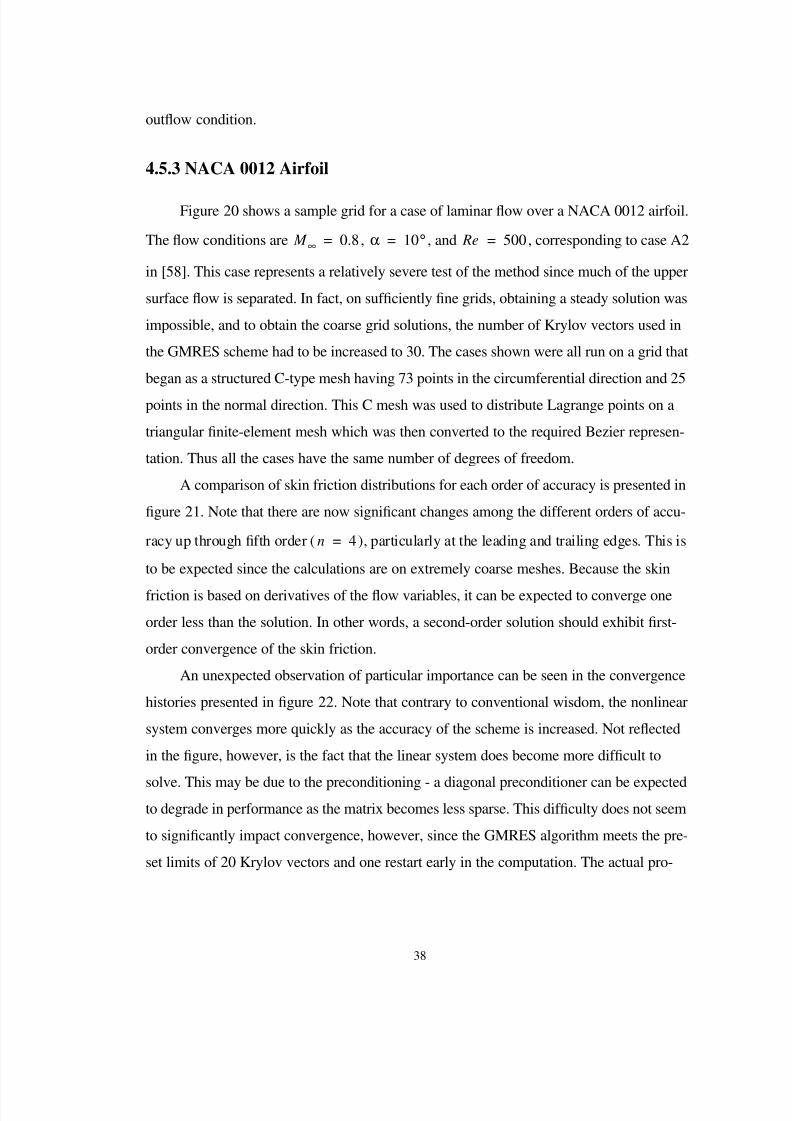
8/8/2019 A Higher Order Accurate Finite Element Method for Viscous Compressible Flows
http://slidepdf.com/reader/full/a-higher-order-accurate-finite-element-method-for-viscous-compressible-flows 46/86
38
outflow condition.
4.5.3 NACA 0012 Airfoil
Figure 20 shows a sample grid for a case of laminar flow over a NACA 0012 airfoil.
The flow conditions are , , and , corresponding to case A2
in [58]. This case represents a relatively severe test of the method since much of the upper
surface flow is separated. In fact, on sufficiently fine grids, obtaining a steady solution was
impossible, and to obtain the coarse grid solutions, the number of Krylov vectors used in
the GMRES scheme had to be increased to 30. The cases shown were all run on a grid that
began as a structured C-type mesh having 73 points in the circumferential direction and 25
points in the normal direction. This C mesh was used to distribute Lagrange points on a
triangular finite-element mesh which was then converted to the required Bezier represen-
tation. Thus all the cases have the same number of degrees of freedom.
A comparison of skin friction distributions for each order of accuracy is presented in
figure 21. Note that there are now significant changes among the different orders of accu-
racy up through fifth order ( ), particularly at the leading and trailing edges. This is
to be expected since the calculations are on extremely coarse meshes. Because the skin
friction is based on derivatives of the flow variables, it can be expected to converge one
order less than the solution. In other words, a second-order solution should exhibit first-
order convergence of the skin friction.
An unexpected observation of particular importance can be seen in the convergence
histories presented in figure 22. Note that contrary to conventional wisdom, the nonlinear
system converges more quickly as the accuracy of the scheme is increased. Not reflected
in the figure, however, is the fact that the linear system does become more difficult to
solve. This may be due to the preconditioning - a diagonal preconditioner can be expected
to degrade in performance as the matrix becomes less sparse. This difficulty does not seem
to significantly impact convergence, however, since the GMRES algorithm meets the pre-
set limits of 20 Krylov vectors and one restart early in the computation. The actual pro-
M ∞ 0.8= α 10°= Re 500=
n 4=
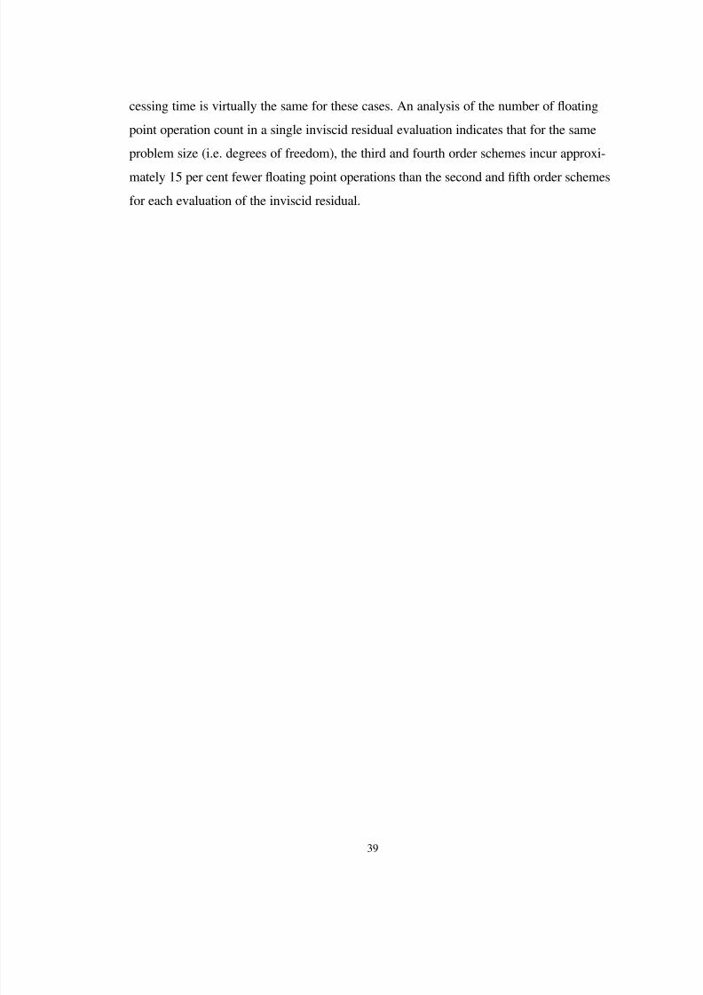
8/8/2019 A Higher Order Accurate Finite Element Method for Viscous Compressible Flows
http://slidepdf.com/reader/full/a-higher-order-accurate-finite-element-method-for-viscous-compressible-flows 47/86
39
cessing time is virtually the same for these cases. An analysis of the number of floating
point operation count in a single inviscid residual evaluation indicates that for the same
problem size (i.e. degrees of freedom), the third and fourth order schemes incur approxi-
mately 15 per cent fewer floating point operations than the second and fifth order schemes
for each evaluation of the inviscid residual.

8/8/2019 A Higher Order Accurate Finite Element Method for Viscous Compressible Flows
http://slidepdf.com/reader/full/a-higher-order-accurate-finite-element-method-for-viscous-compressible-flows 48/86
40
Figure 4. Element data distribution using triangular Bezier patches.
shared points
a) Enforcement of continuity via shared control points (cubic elements depicted).
control points
00
30
1202
211101
10 20 300
9
87
654
321
b) Indexing of control points within an element (cubic element depicted).
ij
inode

8/8/2019 A Higher Order Accurate Finite Element Method for Viscous Compressible Flows
http://slidepdf.com/reader/full/a-higher-order-accurate-finite-element-method-for-viscous-compressible-flows 49/86
41
Figure 5. Boundary element data distribution using Bezier segments.
boundary surface
boundary control points
control points

8/8/2019 A Higher Order Accurate Finite Element Method for Viscous Compressible Flows
http://slidepdf.com/reader/full/a-higher-order-accurate-finite-element-method-for-viscous-compressible-flows 50/86
42
2 . 2
2
1 . 8
1 . 6
1. 4
1. 2
1
0. 8
0.6
0 .5
Figure 6. Computational regions in Ringleb flow domain used for analysis.
Streamlines
Supersonic flow region
Subsonic flow region
Isomach lines
Outflow boundary

8/8/2019 A Higher Order Accurate Finite Element Method for Viscous Compressible Flows
http://slidepdf.com/reader/full/a-higher-order-accurate-finite-element-method-for-viscous-compressible-flows 51/86
43
Figure 7. Generation of finite element meshes for Ringleb flow.
N 6=
n 2=

8/8/2019 A Higher Order Accurate Finite Element Method for Viscous Compressible Flows
http://slidepdf.com/reader/full/a-higher-order-accurate-finite-element-method-for-viscous-compressible-flows 52/86
44
Figure 8. Error norms in subsonic region of Ringleb flow.
Degrees of freedom
8/8/2019 A Higher Order Accurate Finite Element Method for Viscous Compressible Flows
http://slidepdf.com/reader/full/a-higher-order-accurate-finite-element-method-for-viscous-compressible-flows 53/86
45
Degrees of freedom
Figure 9. Error norms in supersonic region of Ringleb flow.

8/8/2019 A Higher Order Accurate Finite Element Method for Viscous Compressible Flows
http://slidepdf.com/reader/full/a-higher-order-accurate-finite-element-method-for-viscous-compressible-flows 54/86
46
Bezier control polygonBezier curve
0.1
1
Figure 10. Geometry and grid for parabolic bump in a channel.
a) Geometry and baseline grid.
b) Sample grid, , . N 2= n 3=
8/8/2019 A Higher Order Accurate Finite Element Method for Viscous Compressible Flows
http://slidepdf.com/reader/full/a-higher-order-accurate-finite-element-method-for-viscous-compressible-flows 55/86
47
-1 0 1 20.3
0.4
0.5
0.6
N=12, n=1N=6, n=2
N=4, n=3N=3, n=4
-1 0 1 20.3
0.4
0.5
0.6
N=12, n=1N=6, n=2FUN2D, N=12FUN2D, N=24
0.4 0.5 0.60.55
0.56
0.57
0.58
0.59
0.6
Figure 11. Surface Mach number distribution for parabolic bump in a channel.
M a c h n u m b e r
x L ⁄
a) Comparison of high order SU/PG schemes.
b) Comparison with second order finite volume scheme.
M a c h n u m b e r
x L ⁄

8/8/2019 A Higher Order Accurate Finite Element Method for Viscous Compressible Flows
http://slidepdf.com/reader/full/a-higher-order-accurate-finite-element-method-for-viscous-compressible-flows 56/86
48
Figure 12. Mach number contours for parabolic bump on a wall.
a) Second order SU/PG scheme.
b) Second order finite volume scheme.

8/8/2019 A Higher Order Accurate Finite Element Method for Viscous Compressible Flows
http://slidepdf.com/reader/full/a-higher-order-accurate-finite-element-method-for-viscous-compressible-flows 57/86
49
Figure 13. Fine grid for inviscid flow over a NACA 0012 airfoil.
a) Fine grid.
c) Coarse grid.
b) Medium grid.
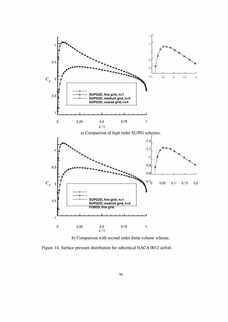
8/8/2019 A Higher Order Accurate Finite Element Method for Viscous Compressible Flows
http://slidepdf.com/reader/full/a-higher-order-accurate-finite-element-method-for-viscous-compressible-flows 58/86
50
0 0.25 0.5 0.75 1
-1
-0.5
0
0.5
1
SUPG2D, fine grid, n=1SUPG2D, medium grid, n=2SUPG2D, coarse grid, n=4
0 0.05 0.1 0.15 0.2
-1.2
-1.1
-1
-0.9
-0.8
-0.7
0 0.25 0.5 0.75 1
-1
-0.5
0
0.5
1
SUPG2D, fine grid, n=1SUPG2D, medium grid, n=2FUN2D, fine grid
0 0.05 0.1 0.15 0.2
-1.2
-1.1
-1
-0.9
-0.8
-0.7
Figure 14. Surface pressure distribution for subcritical NACA 0012 airfoil.
x c ⁄
C p
a) Comparison of high order SU/PG schemes.
b) Comparison with second order finite volume scheme.
x c ⁄
C p
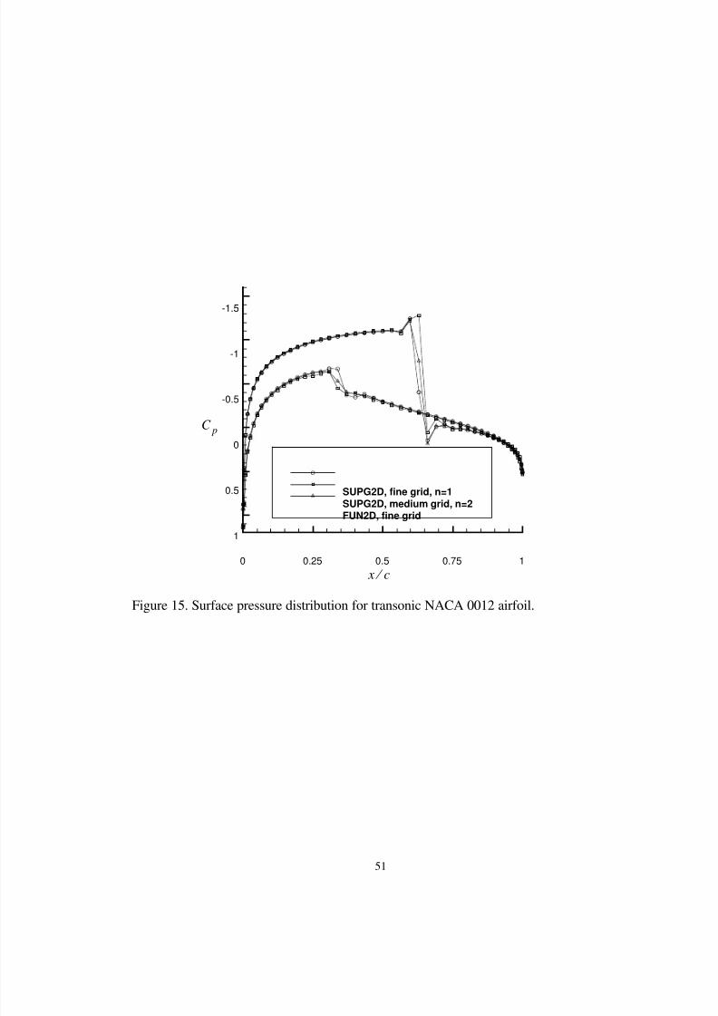
8/8/2019 A Higher Order Accurate Finite Element Method for Viscous Compressible Flows
http://slidepdf.com/reader/full/a-higher-order-accurate-finite-element-method-for-viscous-compressible-flows 59/86
51
0 0.25 0.5 0.75 1
-1.5
-1
-0.5
0
0.5
1
SUPG2D, fine grid, n=1SUPG2D, medium grid, n=2FUN2D, fine grid
Figure 15. Surface pressure distribution for transonic NACA 0012 airfoil.
x c ⁄
C p

8/8/2019 A Higher Order Accurate Finite Element Method for Viscous Compressible Flows
http://slidepdf.com/reader/full/a-higher-order-accurate-finite-element-method-for-viscous-compressible-flows 60/86
52
Figure 16. Solution domain for rotational Couette flow.
r 1
r 2ω1
ω2
a) Geometry.
b) Sample grid.

8/8/2019 A Higher Order Accurate Finite Element Method for Viscous Compressible Flows
http://slidepdf.com/reader/full/a-higher-order-accurate-finite-element-method-for-viscous-compressible-flows 61/86
53
101
102
103
104
10510
-11
10-10
10-9
10-8
10-7
10-6
10-5
10
-4
10-3
10-2
n=1n=2n=3n=4
Figure 17. Error in circumferential velocity for rotational Couette flow.
L2
Degrees of freedom
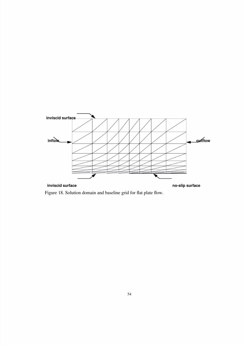
8/8/2019 A Higher Order Accurate Finite Element Method for Viscous Compressible Flows
http://slidepdf.com/reader/full/a-higher-order-accurate-finite-element-method-for-viscous-compressible-flows 62/86
54
Figure 18. Solution domain and baseline grid for flat plate flow.
no-slip surfaceinviscid surface
inflow
inviscid surface
outflow
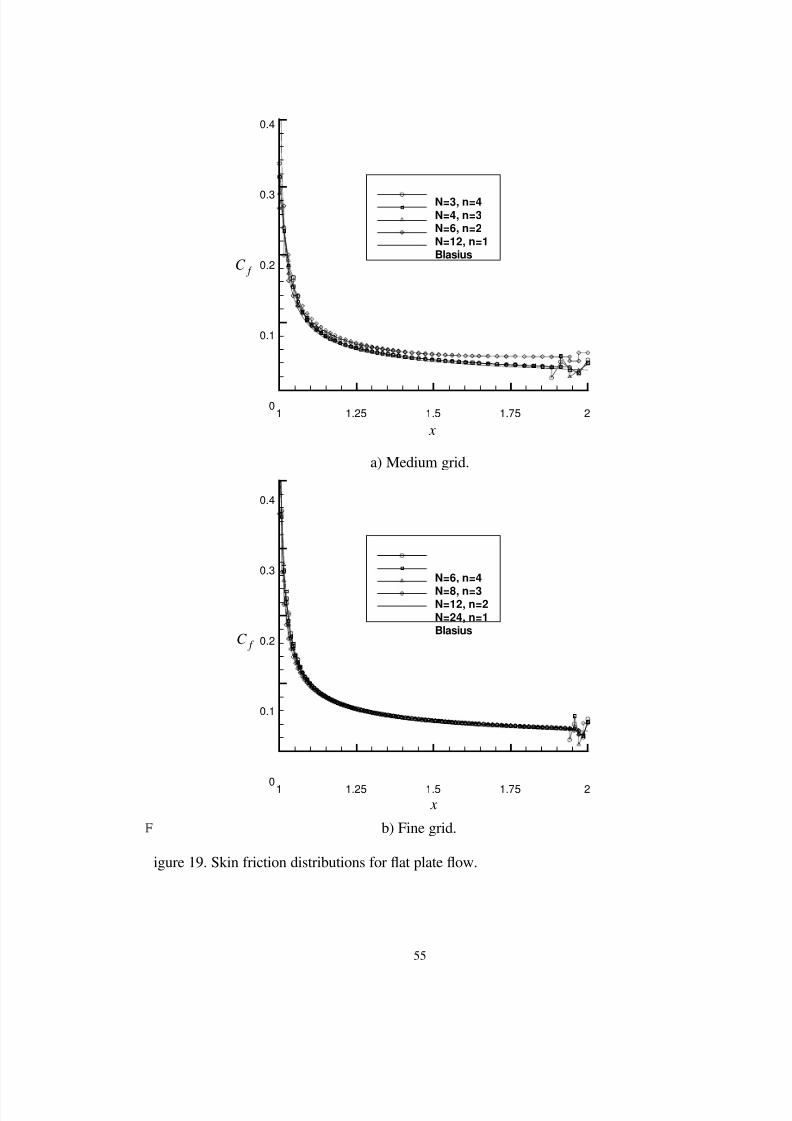
8/8/2019 A Higher Order Accurate Finite Element Method for Viscous Compressible Flows
http://slidepdf.com/reader/full/a-higher-order-accurate-finite-element-method-for-viscous-compressible-flows 63/86
55
1 1.25 1.5 1.75 20
0.1
0.2
0.3
0.4
N=3, n=4N=4, n=3N=6, n=2N=12, n=1Blasius
1 1.25 1.5 1.75 20
0.1
0.2
0.3
0.4
N=6, n=4N=8, n=3N=12, n=2N=24, n=1Blasius
igure 19. Skin friction distributions for flat plate flow.
x
C f
a) Medium grid.
b) Fine grid.
x
C f

8/8/2019 A Higher Order Accurate Finite Element Method for Viscous Compressible Flows
http://slidepdf.com/reader/full/a-higher-order-accurate-finite-element-method-for-viscous-compressible-flows 64/86
56
Figure 20. Sample grid for laminar flow over a NACA 0012 airfoil.

8/8/2019 A Higher Order Accurate Finite Element Method for Viscous Compressible Flows
http://slidepdf.com/reader/full/a-higher-order-accurate-finite-element-method-for-viscous-compressible-flows 65/86
57
0 0.25 0.5 0.75 1-0.2
-0.1
0
0.1
0.2
0.3
0.4
0.5
0.6
n=4n=3n=2n=1
Figure 21. Skin friction distributions for laminar flow over a NACA 0012 airfoil.
x
C f

8/8/2019 A Higher Order Accurate Finite Element Method for Viscous Compressible Flows
http://slidepdf.com/reader/full/a-higher-order-accurate-finite-element-method-for-viscous-compressible-flows 66/86
58
0 100 200 300 400 50010
-12
10-10
10-8
10-6
10-4
10-2
100
n=4n=3n=2n=1
Figure 22. Convergence histories for laminar flow over a NACA 0012 airfoil.
Iteration
R e s i d u a l

8/8/2019 A Higher Order Accurate Finite Element Method for Viscous Compressible Flows
http://slidepdf.com/reader/full/a-higher-order-accurate-finite-element-method-for-viscous-compressible-flows 67/86
59
Chapter 5
Concluding Remarks
The SU/PG method has been applied for the first time to higher-order finite-elementdiscretizations in one and two dimensions. Several test cases involving both subsonic and
transonic inviscid flows in one and two dimensions were investigated as well as several
subsonic laminar flow cases in two dimensions. High order accuracy was confirmed up to
ninth order for one-dimensional flows and up to fifth order for two dimensional inviscid
and laminar flows. The higher order schemes were found to provide significantly more
accurate results using fewer computational resources. An appendix is included in which
the method is applied to three-dimensional inviscid flows. Several important observations
were made based on the results:
1. No modification of the SU/PG scheme is required to achieve high order accuracy. This
essentially means that the order property of the scheme is independent of the formula-
tion of the SU/PG parameter τ provided the original design criteria are met(i.e. that τ
vanishes as the mesh is refined). There are indications from comparisons with a second
order finite volume scheme, that an improved formulation of the τ matrix could further
reduce error levels by a constant factor.
2. Significant improvement of the solution results from using the higher order schemes.
Error norms for Ringleb flow and Couette flow indicate that the high order schemes
outperform the second order scheme even on very coarse meshes. Analysis of opera-
tion counts indicates that based on problem size, the third and fourth order schemes
8/8/2019 A Higher Order Accurate Finite Element Method for Viscous Compressible Flows
http://slidepdf.com/reader/full/a-higher-order-accurate-finite-element-method-for-viscous-compressible-flows 68/86
60
are cheaper to compute than the second order scheme, and that the operation count of
the fifth order scheme is comparable to the second order scheme.
3. Neglecting the Petrov-Galerkin contribution of the viscous terms in the two-dimen-
sional schemes had no impact on the order properties of the scheme. In spite of the
absence of these terms, the error norms for Couette flow converged at high order.
There is the possibility, however, that inclusion of these terms could influence error
levels by a constant factor.
4. The nonlinear system converges more quickly as the order of accuracy is increased for
the same number of degrees of freedom. The linear system converges more slowly, but
processing time is only slightly affected because the linear solver reaches the limit of
its allotted resources per iteration early in the computation. This is contrary to popular
belief that higher-order schemes suffer from convergence problems.
Clearly, the results shown here indicate that higher order schemes can greatly reduce
the computational resources required to compute steady-state aerodynamics of complex
configurations. In order to realize this potential, however, several areas must be explored
in future research.
The primary difficulty in using the higher-order schemes was the generation of suit-
able higher-order discretizations of the flow domain when curved boundaries were
involved. No general solution was found - each case required its own preprocessor to gen-
erate the higher-order finite-element mesh from an existing structured mesh or linear
finite-element mesh. Particularly difficult to generate are meshes that are highly stretched
to compute viscous flows - simply moving the boundary control points to match the sur-
face creates overlapping elements which are unacceptable to the scheme. These problems
are further compounded in three dimensions. To facilitate application of the higher-order
schemes in general, grid generation techniques must be adapted to handle high-order dis-
cretizations and must be more closely tied to geometry definitions (e.g. CAD systems).
This remains as an avenue of future work.
Other issues remaining for future research with the two-dimensional scheme are
improvement of the Petrov-Galerkin parameter τ as discussed in chapter 2 and the incor-

8/8/2019 A Higher Order Accurate Finite Element Method for Viscous Compressible Flows
http://slidepdf.com/reader/full/a-higher-order-accurate-finite-element-method-for-viscous-compressible-flows 69/86
61
poration of the Petrov-Galerkin contribution of the viscous terms, both of which may fur-
ther reduce error levels by a constant factor. The GMRES algorithm with block-diagonal
preconditioning provided adequate convergence of the linear system, but an improved pre-
conditioning scheme could bring gains in efficiency by allowing a larger pseudotime step.
The addition of a turbulence model will allow computation of high Reynolds number
flows. The three-dimensional scheme (presented in appendix A) can benefit from these
same improvements and will also require the addition of viscous terms.

8/8/2019 A Higher Order Accurate Finite Element Method for Viscous Compressible Flows
http://slidepdf.com/reader/full/a-higher-order-accurate-finite-element-method-for-viscous-compressible-flows 70/86
62
References
1. Barth, T. J. and Jesperson, D. C.; “The Design and Application of Upwind Schemes on
Unstructured Meshes,” AIAA 27th Aerospace Sciences Meeting, AIAA 89-0366, January
1989.
2. Whitaker, D. L., Slack, D. C., and Walters, R. W.; “Solution Algorithms for the Two-
Dimensional Euler Equations on Unstructured Meshes,” AIAA 90-0697, 1990.
3. Jameson, A., Baker, T., and Weatherill, N.; “Calculation of Inviscid Transonic Flow
over a Complete Aircraft,” AIAA 24th Aerospace Sciences Meeting, AIAA 86-0103, Janu-
ary 1986.
4. Jameson, A. and Baker, T.; “Improvements to the Aircraft Euler Method,” AIAA 25th
Aerospace Sciences Meeting, AIAA 87-0452, January 1987.
5. Jameson, A. and Mavriplis, D.; “Finite Volume Solution of the Two-Dimensional Euler
Equations on a Regular Triangular Mesh,” AIAA 23rd Aerospace Sciences Meeting, AIAA
85-0435, January 1985.
6. Mavriplis, D. and Jameson, A.; “Multigrid Solution of the Navier-Stokes Equations on
Triangular Meshes,” AIAA Journal, vol. 28, pp. 1415-1425, January 1986.
7. Barth, T. J.; “Numerical Aspects of Computing Viscous High Reynolds Number Flows
on Unstructured Meshes,” AIAA 29th Aerospace Sciences Meeting, AIAA 91-0721, Janu-ary 1991.
8. Barth, T. J. and Frederickson, P. O.; “Higher Order Solution of the Euler Equations on
Unstructured Grids Using Quadratic Reconstruction,” AIAA 90-0013, January 1990.
9. Hu, C. and Shu, C. W.; “Weighted Essentially Non-Oscillatory Schemes on Triangular
8/8/2019 A Higher Order Accurate Finite Element Method for Viscous Compressible Flows
http://slidepdf.com/reader/full/a-higher-order-accurate-finite-element-method-for-viscous-compressible-flows 71/86
63
Meshes,” NASA CR-1998-208459, July 1998.
10. Halt, D. W.; “A Compact High-Order Euler Solver for Unstructured Grids,” Ph.D. dis-
sertation, Washington University, May 1992.
11. Halt, D. W. and Agarwal, R. K.; “A Compact Higher Order Characteristic-Based Euler
Solver for Unstructured Grids,” AIAA 29th Applied Aerodynamics Conference, AIAA
91-3234, September 1991.
12. Zienkiewicz, O. C.; The Finite Element Method , McGraw-Hill Book Company (UK)
Limited, London, 1977.
13. Hughes, T. J. R.; The Finite Element Method: Linear Static and Dynamic Finite Ele-
ment Analysis, Prentice-Hall, Inc., New Jersey, 1987.
14. Baker, A. J. and Pepper, D. W.; Finite Elements 1-2-3, McGraw-Hill, Inc., New York,
1991.
15. Cockburn, B. and Shu, C.-W.; “TVB Runge-Kutta Local Projection Discontinuous
Galerkin Finite Element Method for Conservation Laws II: General Framework,” Mathe-
matics of Computation, vol. 52, pp. 411-435, 1989.
16. Cockburn, B., Lin, S. Y., and Shu, C.-W.; “TVB Runge-Kutta Local Projection Dis-
continuous Galerkin Finite Element Method for Conservation Laws III: One Dimensional
Systems,” Journal of Computational Physics, vol. 84, pp. 90-113, 1989.
17. Cockburn, B. Hou, S., and Shu, C.-W.; “TVB Runge-Kutta Local Projection Discon-
tinuous Galerkin Finite Element Method for Conservation Laws IV: The Multidimen-
sional Case,” Mathematics of Computation, vol. 54, pp. 545-581, 1990.
18. Bey, K. S.; “An HP-Adaptive Discontinuous Galerkin Method for Hyperbolic Conser-
vation Laws,” Ph.D. dissertation, Univ. of Texas at Austin, 1994.
19. Atkins, H. L. and Shu, C.-W.; “Quadrature-Free Implementation of the Discontinuous
Galerkin Method for Hyperbolic Equations,” 2nd AIAA/CEAS Aeroacoustics Conference,
AIAA 96-1683, May 1996.
20. Lowrie, R. B., Roe, P. L. and van Leer, B.; “A Space-Time Discontinuous Galerkin
Method for the Time-Accurate Numerical Solution of Hyperbolic Conservation Laws,”
AIAA 95-1658, 1995.
8/8/2019 A Higher Order Accurate Finite Element Method for Viscous Compressible Flows
http://slidepdf.com/reader/full/a-higher-order-accurate-finite-element-method-for-viscous-compressible-flows 72/86
64
21. Bey, K. S. and Oden, J. T.; “A Runge-Kutta Discontinuous Finite Element Method for
High Speed Flows,” AIAA 10th Computational Fluid Dynamics Conference, AIAA 91-
1575-CP, June 1991.
22. Bassi, F. and Rebay, S.; “Discontinuous Finite Element High Order Accurate Numeri-
cal Solution of the Compressible Navier-Stokes Equations,” ICFD Conference on Numer-
ical Methods in Fluid Dynamics, Bangalor, India, July 1994.
23. Bassi, F. and Rebay, S.; “Accurate 2D Euler Computations by Means of a High-Order
Discontinuous Finite Element Method,” Proceedings of the 14th International Conference
on Numerical Methods in Fluid Dynamics, Oxford, England, April 1995.
24. Brooks, A. N. and Hughes, T. J. R.; “Streamline Upwind/Petrov-Galerkin Formula-
tions for Convection Dominated Flows with Particular Emphasis on the Incompressible
Navier-Stokes Equations,” Computer Methods in Applied Mechanics and Engineering,
vol. 32, pp. 199-259, 1982.
25. Brezzi, F., Franca, L. P., Hughes, T. J. R., and Russa, A.; “Stabilization Techniques and
Subgrid Scales Capturing,” The State of the Art in Numerical Analysis, based on the pro-
ceedings of the Conference on the State of the Art in Numerical Analysis, York, England,
April 1996, IMA Conference Series, Vol. 63 (I.S. Duff and G.A. Watson, eds.), Oxford
University Press, pp. 391-406.
26. Hughes, T. J. R. and Mallet, M.; “A New Finite Element Formulation for Computa-
tional Fluid Dynamics: III. The Generalized Streamline Operator for Multidimensional
Advective-Diffusive Systems,” Computer Methods in Applied Mechanics and Engineer-
ing, vol. 58, pp. 305-328, 1986.
27. Hughes, T. J. R. and Mallet, M.; “A New Finite Element Formulation for Computa-
tional Fluid Dynamics: IV. A Discontinuity-Capturing Operator for Multidimensional
Advective-Diffusive Systems,” Computer Methods in Applied Mechanics and Engineer-
ing, vol. 58, pp. 329-336, 1986.
28. Hughes, T. J. R., Franca, L. P., and Hulbert, G. M.; “A New Finite Element Formula-
tion for Computational Fluid Dynamics: VIII. The Galerkin/Least-Squares Method for
Advective-Diffusive Equations,” Computer Methods in Applied Mechanics and Engineer-
8/8/2019 A Higher Order Accurate Finite Element Method for Viscous Compressible Flows
http://slidepdf.com/reader/full/a-higher-order-accurate-finite-element-method-for-viscous-compressible-flows 73/86
65
ing, vol. 73, pp. 173-189, 1989.
29. Soulaïmani, A. and Fortin, M.; “Finite element solution of compressible viscous flows
using conservative variables,” Computer Methods in Applied Mechanics and Engineering,
No. 118, pp. 319-350, 1994.
30. Franca, L. P., Harari, I., Hughes, T. J. R., Mallet, M., Shakib, F., Spelce, T. E., Chalot,
F., and Tezduyar, T. E.; “A Petrov-Galerkin Finite Element Method for the Compressible
Euler and Navier-Stokes Equations,” Numerical Methods for Compressible Flows - Finite
Difference, Element and Volume Techniques; Proceedings of the Winter Annual Meeting,
American Society of Mechanical Engineers, New York, pp. 19-43, 1986.
31. Brueckner, F. P. and Heinrich, J. C.; “Petrov-Galerkin Finite Element Method for
Compressible Flows,” International Journal for Numerical Methods in Engineering, Vol.
32, pp. 255-274, 1991.
32. Carette, J.-C., Deconinck, H., Paillere, H., and Roe, P. L.; “Multidimensional Upwind-
ing: Its Relation to Finite Elements,” International Journal for Numerical Methods in Flu-
ids, Vol. 20, pp. 935-955, 1995.
33. Paillere, H., Carette, J.-C., and Deconinck, H.; “Multidimensional Upwind and SUPG
Methods for the Solution of the Compressible Flow Equations on Unstructured Grids,” in
von Karman Institute for Fluid Dynamics Lecture Series 1994-05: Computational Fluid
Dynamics, von Karman Institute for Fluid Dynamics, Rhode Saint Genese, Belgium,
1994.
34. Shakib, F.; “Finite Element Analysis of the Compressible Euler and Navier-Stokes
Equations,” Ph.D. dissertation, Stanford University, August 1988.
35. Shakib, F., Hughes, T. J. R., and Johan, Z; A New Finite Element Formulation for
Computational Fluid Dynamics: X. The Compressible Euler and Navier-Stokes Equa-
tions,” Computer Methods in Applied Mechanics and Engineering, vol. 89, pp. 141-219,
1991.
36. Chiocchia, G.; “Exact Solution to Transonic and Supersonic Flows,” Test Cases for
Inviscid Flow Field Methods, AGARD Advisory Report AR-211, May 1985.
37. Chossat, P and Iooss, G.; The Couette-Taylor Problem, Springer-Verlag New York,
8/8/2019 A Higher Order Accurate Finite Element Method for Viscous Compressible Flows
http://slidepdf.com/reader/full/a-higher-order-accurate-finite-element-method-for-viscous-compressible-flows 74/86
66
Inc., 1994.
38. Courant, R., Isaacson, E., and Reeves, M.; “On the Solution of Nonlinear Hyperbolic
Differential Equations by Finite Differences,” Comm. Pure and Applied Mathematics, vol.
5, pp. 243-255.
39. Hughes, T. J. R.; “Multiscale Phenomena: Green’s Functions, the Dirichlet-to-Neu-
mann Formulation, Subgrid Scale Models, Bubbles and the Origins of Stabilized Meth-
ods,” Computer Methods in Applied Mechanics and Engineering, vol. 127, pp. 387-401,
1995.
40. Mizukami, A. and Hughes, T. J. R.; “A Petrov-Galerkin Finite Element Method for
Convection-Dominated Flows: An Accurate Upwinding Technique for Satisfying the
Maximum Principle,” Computer Methods in Applied Mechanics and Engineering, vol. 50,
pp. 181-193, 1985.
41. Casper, J and Carpenter, M. H.; “Computational Considerations for the Simulation of
Shock-Induced Sound,” NASA TM-110222, December 1995.
42. Ames Research Center Staff; “Equations, Tables, and Charts for Compressible Flow,”
NACA Report 1135, 1953.
43. Jansen, K. E., Collis, S. S., Whiting, C. and Shakib, F.; “A Better Consistency for Low-
Order Stabilized Finite Element Methods,” Computer Methods in Applied Mechanics and
Engineering, to appear.
44. Cowper, G. R.; “Gaussian Quadrature Formulas for Triangles,” International Journal
of Numerical Methods in Engineering, vol. 7, pp. 405-408, 1973.
45. Saad, Y., and Schultz, M. H.; “GMRES: A Generalized Minimum Residual Algorithm
for Solving Nonsymmetric Linear Systems,” SIAM Journal of Scientific and Statistical
Computing, vol. 7, pp. 856-869, 1986.
46. Saad, Y.; “Krylov Subspace Techniques, Conjugate Gradients, Preconditioning and
Sparse Matrix Solvers,” in von Karman Institute for Fluid Dynamics Lecture Series 1994-
05: Computational Fluid Dynamics, von Karman Institute for Fluid Dynamics, Rhode
Saint Genese, Belgium, 1994.
47. McHugh, P. R. and Knoll, D. A.; “Comparison of Standard and Matrix-Free Imple-
8/8/2019 A Higher Order Accurate Finite Element Method for Viscous Compressible Flows
http://slidepdf.com/reader/full/a-higher-order-accurate-finite-element-method-for-viscous-compressible-flows 75/86
67
mentations of Several Newton-Krylov Solvers,” AIAA Journal, vol. 32, no. 12, December
1994.
48. Axelsson, O.; Iterative Solution Methods, Cambridge University Press, New York,
1994, pp. 252-371.
49. Chow, E. and Saad, Y.; “Approximate Inverse Preconditioners for General Sparse
Matrices,” University of Minnesota Supercomputing Institute Research Report UMSI 94/
101, May 1994.
50. Chow, E. and Saad, Y.; “Approximate Inverse Preconditioners via Sparse-Sparse Itera-
tions,” SIAM Journal of Scientific Computing, Vol. 19, No. 3, pp. 995-1023, May 1998.
51. Gould, N. I. M. and Scott, J. A.; “Sparse Approximate-Inverse Preconditioners Using
Norm-Minimization Techniques,” SIAM Journal of Scientific Computing, Vol. 19, No. 2,
pp. 605-625, March 1998.
52. Anderson, W. K. and Bonhaus, D. L.; “An Implicit Upwind Algorithm for Computing
Turbulent Flows on Unstructured Grids,” Computers and Fluids, Vol. 23, No. 1, pp. 1-21,
1994.
53. Marcum, D.L. and Weatherill, N.P.; “Unstructured Grid Generation Using Iterative
Point Insertion and Local Reconnection,” AIAA Journal, Vol. 33, No. 9, pp 1619-1625,
September 1995.
54. Marcum, D.L.; “Unstructured Grid Generation for Viscous Flow Applications,” AIAA
33th Applied Aerodynamics Conference, AIAA 95-0212, January 1995.
55. Abbott, I. H. and von Doenhoff, A. E.; Theory of Wing Sections, Dover Publications,
Inc., New York, 1959.
56. Schlichting, H.; Boundary-Layer Theory, translated by Dr. J. Kestin, seventh edition,
McGraw-Hill Book Company, New York, 1979.
57. Volpe, G.; “Performance of Compressible Flow Codes at Low Mach Numbers,” AIAA
Journal, Vol. 31, pp. 49-56, 1993.
58. Institut National de Recherche en Informatique et en Automatique; “GAMM Work-
shop on Numerical Simulation of Compressible Navier-Stokes Flows,” 1985.
59. Jinyun, Y; “Symmetric Gaussian Quadrature Formulae for Tetrahedronal Regions,”

8/8/2019 A Higher Order Accurate Finite Element Method for Viscous Compressible Flows
http://slidepdf.com/reader/full/a-higher-order-accurate-finite-element-method-for-viscous-compressible-flows 76/86
68
Computer Methods in Applied Mechanics and Engineering, vol. 43, 1984, pp. 349-353.
60. Schmitt, V. and Charpin, F.; “Pressure Distributions on the ONERA M6 Wing at Tran-
sonic Mach Numbers,” in Experimental Data Base for Computer Program Assessment ,
AGARD-AR-138, pp. B1-1-B1-44, May 1979.
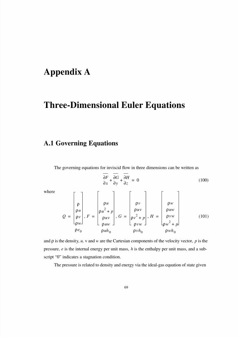
8/8/2019 A Higher Order Accurate Finite Element Method for Viscous Compressible Flows
http://slidepdf.com/reader/full/a-higher-order-accurate-finite-element-method-for-viscous-compressible-flows 77/86
69
Appendix A
Three-Dimensional Euler Equations
A.1 Governing Equations
The governing equations for inviscid flow in three dimensions can be written as
(100)
where
, , , (101)
and ρ is the density, u, v and w are the Cartesian components of the velocity vector, p is the
pressure, e is the internal energy per unit mass, h is the enthalpy per unit mass, and a sub-
script “0” indicates a stagnation condition.
The pressure is related to density and energy via the ideal-gas equation of state given
x∂∂F
y∂∂G
z∂∂ H
+ + 0=
Q
ρρu
ρv
ρw
ρe0
= F
ρu
ρu2
p+
ρuv
ρuw
ρuh0
= G
ρv
ρuv
ρv2
p+
ρvw
ρvh0
= H
ρw
ρuw
ρvw
ρw2
p+
ρwh0
=

8/8/2019 A Higher Order Accurate Finite Element Method for Viscous Compressible Flows
http://slidepdf.com/reader/full/a-higher-order-accurate-finite-element-method-for-viscous-compressible-flows 78/86
70
by
(102)
where γ is the ratio of specific heats.
The nondimensionalization of the equations is identical to that given in chapter 4.
A.2 Finite Element Formulation
The SUPG weak statement corresponding to equation 100 is
. (103)
where w is the Galerkin weight function, A, B and C are the flux Jacobian matrices corre-
sponding to F , G and H , and the matrix τ is defined as in chapter 2. By integrating the
Galerkin terms by parts the weak statement becomes:
(104)
where the fluxes in the boundary integrals are evaluated based on the boundary conditions
as described in chapter 4.
A.3 Solution Methodology
The physical domain Ω is divided into a set of nonoverlapping tetrahedral elements
such that the entire domain is represented. The solution data Q are represented by tet-
p γ 1–( )ρe=
w x∂
∂w A
y∂∂w
B z∂
∂wC + +
τ+ x∂
∂F
y∂∂G
z∂∂ H
+ + Ωd
Ω∫ 0=
w Fn x Gn y Hn z+ +( ) Γ d
Γ ∫ x∂
∂wF
y∂∂w
G z∂
∂w H + +
Ωd
Ω∫ –
x∂∂w
A y∂
∂w B
z∂∂w
C + + τ
x∂∂F
y∂∂G
z∂∂ H
+ + Ωd
Ω∫
+
0=
Ωe
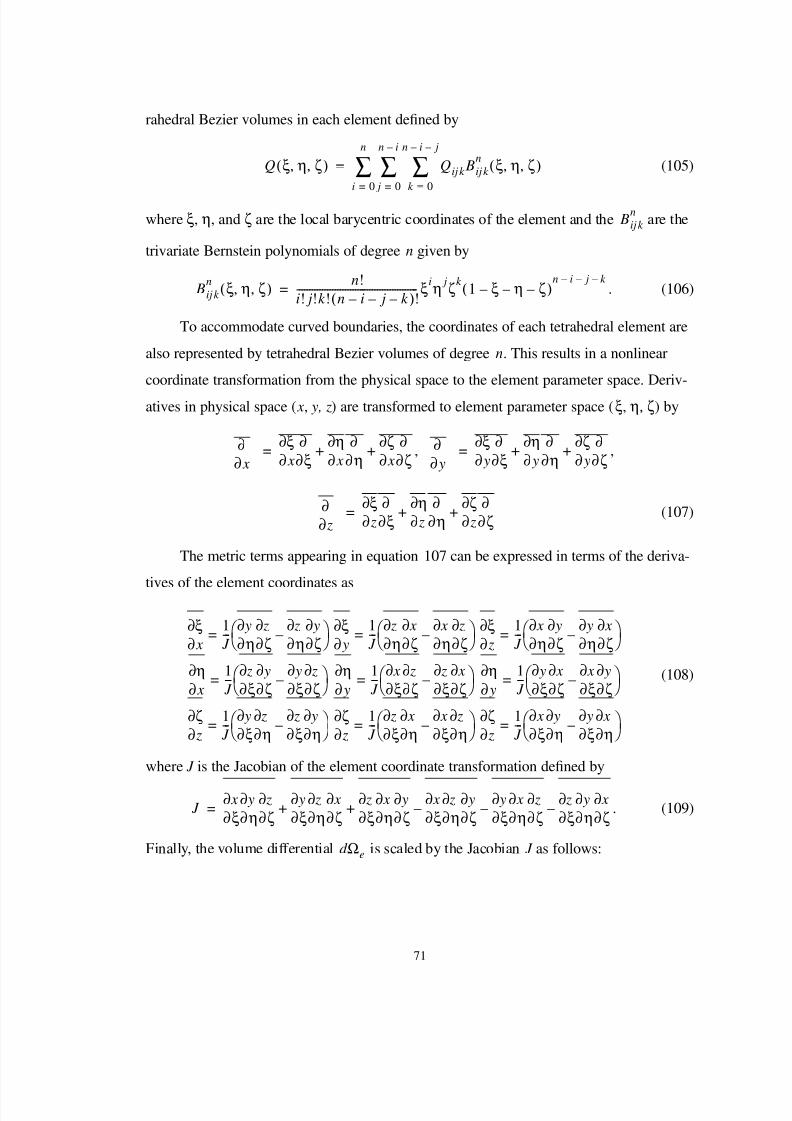
8/8/2019 A Higher Order Accurate Finite Element Method for Viscous Compressible Flows
http://slidepdf.com/reader/full/a-higher-order-accurate-finite-element-method-for-viscous-compressible-flows 79/86
71
rahedral Bezier volumes in each element defined by
(105)
where ξ, η, and ζ are the local barycentric coordinates of the element and the are the
trivariate Bernstein polynomials of degree n given by
. (106)
To accommodate curved boundaries, the coordinates of each tetrahedral element are
also represented by tetrahedral Bezier volumes of degree n. This results in a nonlinear
coordinate transformation from the physical space to the element parameter space. Deriv-atives in physical space ( x, y, z) are transformed to element parameter space (ξ, η, ζ) by
, ,
(107)
The metric terms appearing in equation 107 can be expressed in terms of the deriva-
tives of the element coordinates as
(108)
where J is the Jacobian of the element coordinate transformation defined by
. (109)
Finally, the volume differential is scaled by the Jacobian J as follows:
Q ξ η ζ, ,( ) Qij k Bij k
n ξ η ζ, ,( )k 0=
n i– j–
∑ j 0=
n i–
∑i 0=
n
∑=
Bij k
n
Bij k
n ξ η ζ, ,( ) n!
i! j!k ! n i– j– k –( )!------------------------------------------------ξiη jζk
1 ξ– η– ζ–( )n i– j– k –
=
x∂∂
x∂∂ξ
ξ∂∂
x∂∂η
η∂∂
x∂∂ζ
ζ∂∂
+ += y∂∂
y∂∂ξ
ξ∂∂
y∂∂η
η∂∂
y∂∂ζ
ζ∂∂
+ +=
z∂∂
z∂∂ξ
ξ∂∂
z∂∂η
η∂∂
z∂∂ζ
ζ∂∂
+ +=
x∂∂ξ 1
J ---
η∂∂ y
ζ∂∂ z
η∂∂ z
ζ∂∂ y
– =
y∂∂ξ 1
J ---
η∂∂ z
ζ∂∂ x
η∂∂ x
ζ∂∂ z
– =
z∂∂ξ 1
J ---
η∂∂ x
ζ∂∂ y
η∂∂ y
ζ∂∂ x
– =
x∂∂η 1
J ---
ξ∂∂ z
ζ∂∂ y
ξ∂∂ y
ζ∂∂ z
– =
y∂∂η 1
J ---
ξ∂∂ x
ζ∂∂ z
ξ∂∂ z
ζ∂∂ x
– =
y∂∂η 1
J ---
ξ∂∂ y
ζ∂∂ x
ξ∂∂ x
ζ∂∂ y
– =
z∂∂ζ 1
J ---
ξ∂∂ y
η∂∂ z
ξ∂∂ z
η∂∂ y
– =
z∂∂ζ 1
J ---
ξ∂∂ z
η∂∂ x
ξ∂∂ x
η∂∂ z
– =
z∂∂ζ 1
J ---
ξ∂∂ x
η∂∂ y
ξ∂∂ y
η∂∂ x
– =
J ξ∂
∂ xη∂
∂ yζ∂
∂ zξ∂
∂ yη∂
∂ zζ∂
∂ xξ∂
∂ zη∂
∂ xζ∂
∂ yξ∂
∂ xη∂
∂ zζ∂
∂ y–
ξ∂∂ y
η∂∂ x
ζ∂∂ z
–ξ∂
∂ zη∂
∂ yζ∂
∂ x–+ +=
Ωed

8/8/2019 A Higher Order Accurate Finite Element Method for Viscous Compressible Flows
http://slidepdf.com/reader/full/a-higher-order-accurate-finite-element-method-for-viscous-compressible-flows 80/86
72
(110)
Continuity of the solution across element interfaces is enforced by sharing control
points along the interfaces as illustrated in figure 23a. The indexing in equation
105 is converted to a single index as shown in figure 23b by the following function:
(111)
The boundary Γ of the domain Ω is divided into a finite number of triangular ele-
ments , each of which corresponds to the face of a tetrahedral element adjoining the
boundary. The coordinates and data on each of these elements is represented by a triangu-
lar Bezier patch of degree n as described in chapter 4. Integrals over the boundary Γ can
now be written as sums of integrals over individual boundary elements. These element
integrals are transformed into integrals over the local element parameter space.
The polynomial expression of the boundary element coordinates gives rise to a con-
tinuously varying unit normal along curved elements. The components of the element nor-
mal vector , and are given by
, , (112)
Boundary element integrals are transformed according to
(113)
where
(114)
Upon substitution of the foregoing domain and boundary transformations, the weak
statement (equation 104) can now be written as
Ωed J ξ η ζd d d =
i j k , ,( )
inode k 3n2
12n 11 3nk – 6k – k 2
+ + +( ) 6 ⁄ j 2n 2k j–– 3+( ) 2 ⁄ i+ +=
Γ e
n x n y n z
n x ξ∂∂ z
η∂∂ y
ξ∂∂ y
η∂∂ z
–= n y ξ∂∂ x
η∂∂ z
ξ∂∂ z
η∂∂ x
–= n z ξ∂∂ y
η∂∂ x
ξ∂∂ x
η∂∂ y
–=
f x y z, ,( ) Γ ed
Γ e∫ f x ξ η,( ) y ξ η,( ) z ξ η,( ),,[ ] R ξ ηd d
0
1 η–
∫ 0
1
∫ =
Rξ∂
∂ zη∂
∂ yξ∂
∂ yη∂
∂ z–
2
ξ∂∂ x
η∂∂ z
ξ∂∂ z
η∂∂ x
–
2
ξ∂∂ y
η∂∂ x
ξ∂∂ x
η∂∂ y
–
2
+ +=

8/8/2019 A Higher Order Accurate Finite Element Method for Viscous Compressible Flows
http://slidepdf.com/reader/full/a-higher-order-accurate-finite-element-method-for-viscous-compressible-flows 81/86
73
(115)
where
, , (116)
are the transformed inviscid flux vectors and , and are the corresponding flux Jaco-
bians.
The integrals appearing in equation 115 are evaluated numerically using the Gauss-
ian quadrature rules of [59] for tetrahedral elements and [44] for the triangular elements
on the boundary. Availability of quadrature rules for tetrahedral and triangular elements
limits the scheme to fifth order accuracy.
The solution Q is obtained using a Newton-Krylov scheme as described in chapter 4.
The only difference is the preconditioner, which is still of block-diagonal form and is
given by
(117)
w Fn x Gn y Hn z+ +( ) R ξ ηd d
0
1 η–
∫ 0
1
∫ Γ e∑
ξ∂∂w
F ˜ η∂∂w
G ζ∂∂w
H ˜+ + J ξ η ζd d d 0
1 η– ζ–
∫ 0
1 ζ–
∫ 0
1
∫ –
ξ∂∂w
Aη∂
∂w B
ζ∂∂w
C ˜+ + τ A
ξ∂∂Q
Bη∂
∂QC ˜
ζ∂∂Q
+ + J ξ η ζd d d
0
1 η– ζ–
∫ 0
1 ζ–
∫ 0
1
∫ +
Ωe∑
+
0=
F ˜ x∂
∂ξF
y∂∂ξ
G z∂
∂ξ H + += G
x∂∂η
F y∂
∂ηG
z∂∂η
H + += G x∂
∂ζF
y∂∂ζ
G z∂
∂ζ H + +=
A B C ˜
Qm∂∂ Rm
Bij k
n An x Bn y Cn z+ +( ) Bij k
n R ξ ηd d
0
1 η–
∫ 0
1
∫ Γ e∑
ξ∂∂ Bij k
n
Aη∂
∂ Bij k
n
Bζ∂
∂ Bij k
n
C ˜+ +
Bij k
n J ξ η ζd d d
0
1 η– ζ–
∫ 0
1 ζ–
∫ 0
1
∫ –
ξ∂∂ B
ij k
n
A η∂∂ B
ij k
n
B ζ∂∂ B
ij k
n
C ˜+ +
τ A ξ∂∂ B
ij k
n
B η∂∂ B
ij k
n
C ˜ ζ∂∂ B
ij k
n
+ +
J ξ η ζd d d 0
1 η– ζ–
∫ 0
1 ζ–
∫ 0
1
∫
+Ωe
∑
+≈
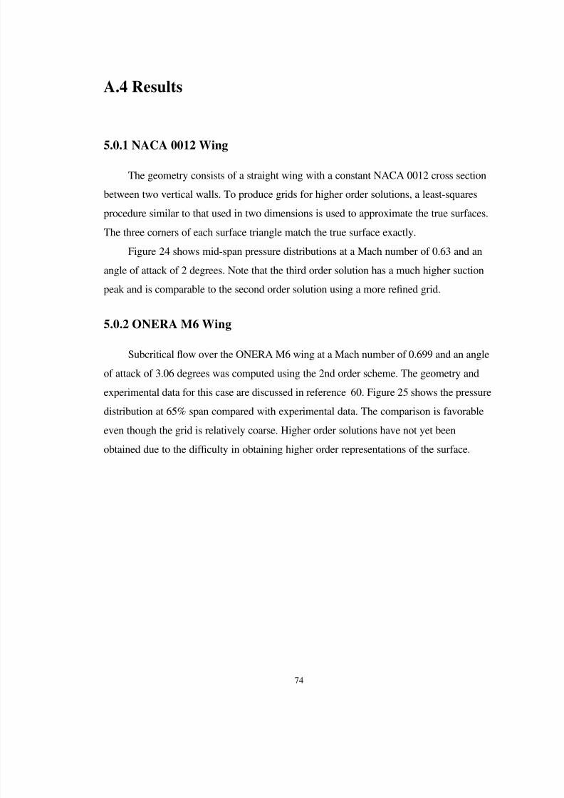
8/8/2019 A Higher Order Accurate Finite Element Method for Viscous Compressible Flows
http://slidepdf.com/reader/full/a-higher-order-accurate-finite-element-method-for-viscous-compressible-flows 82/86
74
A.4 Results
5.0.1 NACA 0012 Wing
The geometry consists of a straight wing with a constant NACA 0012 cross section
between two vertical walls. To produce grids for higher order solutions, a least-squares
procedure similar to that used in two dimensions is used to approximate the true surfaces.
The three corners of each surface triangle match the true surface exactly.
Figure 24 shows mid-span pressure distributions at a Mach number of 0.63 and an
angle of attack of 2 degrees. Note that the third order solution has a much higher suctionpeak and is comparable to the second order solution using a more refined grid.
5.0.2 ONERA M6 Wing
Subcritical flow over the ONERA M6 wing at a Mach number of 0.699 and an angle
of attack of 3.06 degrees was computed using the 2nd order scheme. The geometry and
experimental data for this case are discussed in reference 60. Figure 25 shows the pressure
distribution at 65% span compared with experimental data. The comparison is favorableeven though the grid is relatively coarse. Higher order solutions have not yet been
obtained due to the difficulty in obtaining higher order representations of the surface.

8/8/2019 A Higher Order Accurate Finite Element Method for Viscous Compressible Flows
http://slidepdf.com/reader/full/a-higher-order-accurate-finite-element-method-for-viscous-compressible-flows 83/86
75
Figure 23. Element data distribution using triangular Bezier patches.
shared points
a) Enforcement of continuity via shared control points (quadratic elements depicted).
control points
000
002
011
020
001
110010
100 200
101
0
9
8
5
6
43
7
21
b) Indexing of control points within an element (quadratic element depicted).
ij k
inode

8/8/2019 A Higher Order Accurate Finite Element Method for Viscous Compressible Flows
http://slidepdf.com/reader/full/a-higher-order-accurate-finite-element-method-for-viscous-compressible-flows 84/86
76
0 0.25 0.5 0.75 1
-1.5
-1
-0.5
0
0.5
1
N=2, n=1N=1, n=2N=3, n=1
Figure 24. Mid-span surface pressure distribution for NACA 0012 wing.
C p
x c ⁄
8/8/2019 A Higher Order Accurate Finite Element Method for Viscous Compressible Flows
http://slidepdf.com/reader/full/a-higher-order-accurate-finite-element-method-for-viscous-compressible-flows 85/86
77
0 0.25 0.5 0.75 1
-1.6
-1.4
-1.2
-1
-0.8
-0.6
-0.4
-0.2
0
0.2
0.4
0.6
0.8
1
ExperimentComputation
Figure 25. Surface pressure distribution for ONERA M6 wing at 65% span.
C p
x c ⁄
8/8/2019 A Higher Order Accurate Finite Element Method for Viscous Compressible Flows
http://slidepdf.com/reader/full/a-higher-order-accurate-finite-element-method-for-viscous-compressible-flows 86/86
Vita
Daryl L. Bonhaus was born December 11, 1967 in Cincinnati, Ohio. He graduated
from Elder High School in Cincinnati in June of 1985 and received a B.S. in Aerospace
Engineering in June of 1990 at the University of Cincinnati. Upon graduation, he began
working at the Langley Research Center of the National Aeronautics and Space Adminis-
tration in Hampton, Virginia. He attained a M.S. in Fluid Mechanics and Thermal Sci-
ences from the George Washington University in September of 1993. Daryl continues to
work for the Langley Research Center.