slow viscous flows lecture notespeople.seas.harvard.edu/~colinrmeyer/slow viscous flows...

Slow Viscous FlowsLecture Notes

Colin Meyer

Contents

1 Lecture on 5 October 2012 31.1 Newtonian Fluids . . . . . . . . . . . . . . . . . . . . . . . . . . . . . . . . . . . . . . . . 31.2 Boundary Conditions . . . . . . . . . . . . . . . . . . . . . . . . . . . . . . . . . . . . . . 3

2 Lecture on 8 October 2012 42.1 Stokes Equations . . . . . . . . . . . . . . . . . . . . . . . . . . . . . . . . . . . . . . . . 42.2 Simple Properties . . . . . . . . . . . . . . . . . . . . . . . . . . . . . . . . . . . . . . . . 4

3 Lecture on 10 October 2012 63.1 Three Theorems Based on Dissipation Integrals . . . . . . . . . . . . . . . . . . . . . . . . 63.2 Representation By Potentials . . . . . . . . . . . . . . . . . . . . . . . . . . . . . . . . . 7

4 Lecture on 12 October 2012 74.1 Papkovich-Neuber Representation . . . . . . . . . . . . . . . . . . . . . . . . . . . . . . . 74.2 Solutions For Points and Spheres . . . . . . . . . . . . . . . . . . . . . . . . . . . . . . . . 84.3 Spherical Harmonic Functions . . . . . . . . . . . . . . . . . . . . . . . . . . . . . . . . . 84.4 Tensor Derivatives . . . . . . . . . . . . . . . . . . . . . . . . . . . . . . . . . . . . . . . 94.5 True and Pseudo Tensors . . . . . . . . . . . . . . . . . . . . . . . . . . . . . . . . . . . . 9

5 Lecture on 15 October 2012 95.1 Solution due to a Point Force (Stokeslet, Green’s function) . . . . . . . . . . . . . . . . . . 95.2 Source Flow . . . . . . . . . . . . . . . . . . . . . . . . . . . . . . . . . . . . . . . . . . . 115.3 Dipoles, Stresslets, and Rotlets . . . . . . . . . . . . . . . . . . . . . . . . . . . . . . . . . 11

6 Lecture on 15 October 2012 136.1 Rigid Sphere with Prescribed Velocity . . . . . . . . . . . . . . . . . . . . . . . . . . . . . 13

7 Lecture on 17 October 2012 147.1 The Motion of Rigid Particles . . . . . . . . . . . . . . . . . . . . . . . . . . . . . . . . . 14

7.1.1 The Resistance Matrix . . . . . . . . . . . . . . . . . . . . . . . . . . . . . . . . . 147.1.2 Reciprocal Theorem . . . . . . . . . . . . . . . . . . . . . . . . . . . . . . . . . . 147.1.3 Grand Resistance Matrix . . . . . . . . . . . . . . . . . . . . . . . . . . . . . . . . 15

7.2 Faxen Relations . . . . . . . . . . . . . . . . . . . . . . . . . . . . . . . . . . . . . . . . . 15

8 Lecture on 20 October 2012 168.1 Integral Representations . . . . . . . . . . . . . . . . . . . . . . . . . . . . . . . . . . . . 16

8.1.1 Basic Integral Identity . . . . . . . . . . . . . . . . . . . . . . . . . . . . . . . . . 168.1.2 Far-Field of a Moving Body . . . . . . . . . . . . . . . . . . . . . . . . . . . . . . 17

9 Lecture on 22 October 2012 179.1 Slender Body Theory . . . . . . . . . . . . . . . . . . . . . . . . . . . . . . . . . . . . . . 17

10 Lecture on 24 October 2012 1810.1 Slender Body Theory continued . . . . . . . . . . . . . . . . . . . . . . . . . . . . . . . . 18

10.1.1 Straight Rod in Translation . . . . . . . . . . . . . . . . . . . . . . . . . . . . . . 18

1

11 Lecture on 26 October 2012 1911.1 Marangoni Flows . . . . . . . . . . . . . . . . . . . . . . . . . . . . . . . . . . . . . . . . 19

11.1.1 Boundary Conditions with Surface Tension . . . . . . . . . . . . . . . . . . . . . . 1911.2 Thermophoresis . . . . . . . . . . . . . . . . . . . . . . . . . . . . . . . . . . . . . . . . . 19

11.2.1 Scaling Argument . . . . . . . . . . . . . . . . . . . . . . . . . . . . . . . . . . . . 2011.3 Thermal Problem . . . . . . . . . . . . . . . . . . . . . . . . . . . . . . . . . . . . . . . . 20

12 Lecture on 2 November 2012 2012.1 Thermophoresis continued . . . . . . . . . . . . . . . . . . . . . . . . . . . . . . . . . . . 2012.2 Surfactant Concentration . . . . . . . . . . . . . . . . . . . . . . . . . . . . . . . . . . . . 22

13 Lecture on 5 November 2012 2313.1 Deformation of Drops . . . . . . . . . . . . . . . . . . . . . . . . . . . . . . . . . . . . . . 2413.2 Small Deformations . . . . . . . . . . . . . . . . . . . . . . . . . . . . . . . . . . . . . . . 24

14 Lecture on 5 November 2012 2514.1 Larger Deformations . . . . . . . . . . . . . . . . . . . . . . . . . . . . . . . . . . . . . . 25

14.1.1 Large Deformations with λ1 . . . . . . . . . . . . . . . . . . . . . . . . . . . . 25

15 Lecture on 7 November 2012 2615.1 The Raleigh Instability . . . . . . . . . . . . . . . . . . . . . . . . . . . . . . . . . . . . . 26

16 Lecture on 9 November 2012 2816.1 Long Thin Flows I: Lubrication Theory . . . . . . . . . . . . . . . . . . . . . . . . . . . . 28

17 Lecture on 12 November 2012 2917.1 Viscous Drop Approaching a Plane Wall . . . . . . . . . . . . . . . . . . . . . . . . . . . 2917.2 Dimple Drainage Problem . . . . . . . . . . . . . . . . . . . . . . . . . . . . . . . . . . . 33

18 Lecture on 14 November 2012 3418.1 Gravity Current on an Inclined Plane . . . . . . . . . . . . . . . . . . . . . . . . . . . . . 3418.2 Axisymmetric Horizontal Gravity Current . . . . . . . . . . . . . . . . . . . . . . . . . . . 3618.3 Similarity Solutions . . . . . . . . . . . . . . . . . . . . . . . . . . . . . . . . . . . . . . . 38

18.3.1 Diffusion from a Spherical Heat Pulse . . . . . . . . . . . . . . . . . . . . . . . . . 38

19 Lecture on 16 November 2012 3819.1 Long Thin Flows II: Extensional Flow . . . . . . . . . . . . . . . . . . . . . . . . . . . . . 38

19.1.1 Steady Flow . . . . . . . . . . . . . . . . . . . . . . . . . . . . . . . . . . . . . . . 4019.1.2 Transient Evolution . . . . . . . . . . . . . . . . . . . . . . . . . . . . . . . . . . . 41

20 Lecture on 23 November 2012 4220.1 Long Thin Flows III: Two Fluid Case . . . . . . . . . . . . . . . . . . . . . . . . . . . . . 42

20.1.1 Toffee Stretch Regime . . . . . . . . . . . . . . . . . . . . . . . . . . . . . . . . . 4320.1.2 Sliding Plate . . . . . . . . . . . . . . . . . . . . . . . . . . . . . . . . . . . . . . 43

20.2 Internal Shear . . . . . . . . . . . . . . . . . . . . . . . . . . . . . . . . . . . . . . . . . . 4420.2.1 Nose Push . . . . . . . . . . . . . . . . . . . . . . . . . . . . . . . . . . . . . . . . 44

21 Lecture on 26 November 2012 4421.1 Pigs: Rigid Particle in a Tube . . . . . . . . . . . . . . . . . . . . . . . . . . . . . . . . . 44

22 Lecture on 28 November 2012 4622.1 Slug: Long Bubble In a Tube . . . . . . . . . . . . . . . . . . . . . . . . . . . . . . . . . 46

22.1.1 Nose Region . . . . . . . . . . . . . . . . . . . . . . . . . . . . . . . . . . . . . . . 4722.1.2 Tail Region . . . . . . . . . . . . . . . . . . . . . . . . . . . . . . . . . . . . . . . 48

2

1 Lecture on 5 October 2012

Infinitesimal fluid particles assumed to have a well defined density, ρ(x,t), pressure, p(x,t), and velocity,u(x,t), where x is the position of the particle at time t when you observe it.

The Total Derivative is defined asD

Dt=∂

∂t+u·∇.

Mass Conservation is the statement that∂ρ

∂t+∇·(ρu)=

Dρ

Dt+ρ(∇·u)=0.

For an Incompressible fluid,Dρ

Dt=0−→ ∇·u=0 .

Stress: the stress, τ is a Force/Unit Area acting across a surface (normal). By considering a fluidtetrahedron, it can be shown that τ is linearly related to the normal n of the surface as in

τ=σ·n,where σ is the Stress Tensor, a second rank tensor. Here the sign convention is that n points outwardand τ is the stress exerted by the outside onto the inside.

An angular momentum balance shows thatσ=σT−→σij=σji.

1

The Momentum Equation can then be written directly from Newton’s second law as

ρ

(∂u

∂t+u·∇u

)=F+∇·σ,

Mass×Acceleration=Body Forces+Surface Forces.The Rate of Viscous Dissipation, D is

D=

∫

V

σijeijdV =

∫

V

σ :e dV ,

where

eij=1

2

(∂ui∂xj

+∂uj∂xi

)

is the Strain Rate Tensor and the symmetric part of the Velocity Gradient Tensor, ∇u.1.1 Newtonian Fluids

Stresses are produced by the deformation of the fluid. The relationship between σij and the deformationrate ∂ui/∂xj is local, linear, instantaneous, isotropic. Thus,

σ=−pI+2µe→σij=−pδij+2µeijInternal viscosity is due to the collision of molecules. Linear implies that strain rates are small comparedto typical velocity fluctuations.

Examples of non-Newtonian fluids are: Paint which is shear thinning. Cheesy soup has a history of stress.All fluids in this class will be Newtonian.

For an incompressible Newtonian fluid and uniform viscosity, the Navier-Stokes Equations are

ρ

(∂u

∂t+u·∇u

)= F−∇p+µ∇2u

∇·u = 0.Often F=∇φ and can be incorporated into a modified pressure.

1.2 Boundary Conditions

Kinematic Boundary Conditions At a fluid-fluid interface[u·n]=0, (mass conservation)

[u∧n]=0, (avoid infinite stress)where the brackets indicate matching across the interface.Stationary Rigid Boundary An impermeable boundary gives

u·n=0 (no flux)u∧n=0 (no slip)

1except in magnetic fluids.

3

Dynamic Boundary Conditions If there is no surface tension[σ·n]=0.

With surface tension[σ·n]=γκn−∇sγ,

where γ is the coefficient of surface tension, κ=∇s·n is the curvature of the interface, and ∇s=(I−nn

)∇

is the gradient in the surface.Reynolds Number Suppose U , L, and T=L/U are typical velocity, length, and time scales. Scaling theinertial terms over the viscous terms from the Navier-Stokes Equations we find that

ρu·∇u∼ρU2

Linertial terms

µ∇2u∼µ UL2

viscous stress

Re=ρUL

µ=UL

ν=

inertial forces

viscous stressesThe Kinematic Viscosity is defined as ν=µ/ρ For Re<<1, we can simplify the Navier-Stokes Equationsto the Stokes Equations

µ∇2u = ∇p−F∇·u = 0.

These equations are useful for fluids with very large viscosities, e.g. magma or molten glass, flows with smalllength scales like microfluidics and microorganisms, or long thin flows like paint on a wall.


Notes on the Reynolds Number

1. ∇·u and ∇2u may not involve the same length scale L. For example, lubrication theory (see Lecture16). The thickness of the fluid is much smaller than any horizontal length scale.

2. L may vary in the flow. For example, far-field flow past a body.

3. T may not be L/U if there is an externally imposed time scale such as 1/f for oscillations.

2.1 Stokes Equations

∇·σ=µ∇2u−∇p = −F∇·u = 0.

2.2 Simple Properties

1. Instantaneous: no ∂/∂t term means no time evolution. Flow only knows current boundary conditionsand applied forces. Flow responds immediately to changes, has no inertia and no memory. StokesEquations problems are Boundary Value Problems.

2. Linear: Due to the linearity of the partial differential equations, the response is proportional to theforcing. Furthermore, solutions can be superimposed for a given geometry.

3. Reversible: By changing the sign of all the forces changes the sign of the velocity, u. Thus, reversingthe forces and history of application, all fluid particles retrace their paths exactly. Can be used with asymmetry argument to rule out flow behaviors. For example, a particle next to a wall will not migratebecause if you reverse the forces and then reflect the picture back across the x-axis the horizontalcomponent of the velocity will point in the opposite direction.

4. Forces and Couples Balance: No inertia means that∇·σ+F=0, (1)

and by integrating and using Stoke’s theorem (Divergence theorem) we have a consistency conditionon the stress boundary conditions ∫

∂V

σ·n dS+

∫

V

F dV =0.

4

A consistency condition on the velocity boundary conditions (in the absence of a fluid source) is

∇·u=0→∫

∂V

u·n dS=0. (2)

Likewise, for balance of couples (torques) the consistency condition is∫

∂V

x∧σ·n dS+

∫

V

x∧F dV =0.

This can be derived by taking the cross product of equation 1. Writing it in index notation we have

εijkxj∂σkl∂xl

+εijkxjFk=0.

Rewriting the first term as the divergence of the wedge of x and σ and then integrating over the volume∫

V

∇·(x∧σ·n

)dV +

∫

V

x∧F dV ,

and the first term can be rewritten to fit the form as before using the Divergence theorem.

5. Work Balances Dissipation: No inertia, no angular momentum, and no kinetic energy gives

Dissipation=D=2µ

∫

V

eijeij dV

Using the definition of the stress tensor, σij we have

D=2µ

∫

V

eijeij dV =

∫

V

(σij+pδij)eij dV =

∫

V

σijeij+peii dV =

∫

V

σijeij dV ,

because eii = 0 and thus we arrive at the same expression as before. The remaining term can besimplified because of the symmetry of the stress tensor

σijeij=σij∂ui∂xj

The proof of this fact follows

Proof.

σijeij =σij2

(∂ui∂xj

+∂uj∂xi

)

=1

2

(σij∂ui∂xj

+σji∂uj∂xi

)(symmetry of σij)

=1

2

(σij∂ui∂xj

+σij∂ui∂xj

)(relabeling indices)

= σij∂ui∂xj

Using this fact, we have

D=

∫

V

σij∂ui∂xj

dV =

∫

V

∂

∂xj(ui·σij)−ui

∂σij∂xj

dV .

Invoking equation 1 and the Divergence theorem we find that

D=

∫

∂V

u·σ·n dS+

∫

V

u·F dV .

Thus, dissipation balances work and all work is viscously dissipated immediately.

Lemma 1. If uI is an incompressible flow (i.e. ∇·uI =0) and uS is a Stokes flow with body force FS (suchthat ∇·σS=−FS) then

2µ

∫

V

eIijeSij dV =

∫

∂V

uIiσSijnj dS+

∫

V

uIiFSi dV .

5

Proof. Like the previous derivation for the dissipation we can expand eSij from the definition of the stresstensor. Thus,

2µ

∫

V

eIijeSij dV =

∫

V

eIijσSij dV =

∫

V

∂uIi∂xj

σSij dV =

∫

V

∂

∂xj

(uIiσ

Sij

)−uIi

∂σSij∂xj

dV

Expanding out,

2µ

∫

V

eIijeSij dV =

∫

V

uIiσSijnj dS+

∫

V

uIiFSi dV.


3.1 Three Theorems Based on Dissipation Integrals

Theorem 1. (Uniqueness Theorem) If u1 and u2 are Stokes flows with the same boundary conditionsand body forces f1=f2 in V and either u1=u2 or σ1·n=σ2·n and on ∂V then u∗=u2−u2 is also a Stokes

flow (by linearity). Then, f∗=0 in V and either u∗=0 or σ∗·n=0 on ∂V . Then from Lemma 1.

2µ

∫

V

e∗ :e∗ dV =

∫

∂V

u∗·σ∗·n dS+

∫

V

u∗·f∗ dV =0,

where f∗=0 and either u∗=0 or σ∗·n=0, thuse∗=0 (no strain rate),

This means that u∗ is a solid body motion of the form U+Ω∧x and therefore u1=u2 (unique solution).

Theorem 2. (Reciprocal Theorem) If u1 and u2 are Stokes flows in a certain domain, then∫

V

u1·σ2·n dS+

∫

V

u1·f2 dV =

∫

V

u2·σ1·n dS+

∫

V

u2·f1 dV,Work done by flow 1 against forces 2 is the same as flow 2 against forces 1. Can deduce information abouta flow you know nothing about from a flow you know everything about.

Proof. Starting with

2µ

∫

V

e1 :e2 dV =

∫

V

u1·σ2·n dS+

∫

V

u1·f2 dV =

∫

V

u2·σ1·n dS+

∫

V

u2·f1 dV,by Lemma 1.

Theorem 3. Minimum Dissipation Theorem Of all of the flows in a certain domain, satisfying thegiven velocity boundary conditions and ∇·u=0, the dissipation is minimized by the Stokes flow uS with fS=0

Proof.

0≤2µ

∫

V

(e−eS

):(e−eS

)dV =2µ

∫

V

(e :e−eS :eS

)dV +4µ

∫

V

(eS−e

):eS dV, (3)

which can be seen from

2µ

∫

V

eijeij−2eijeSij+e

Sije

Sij dV = 2µ

∫

V

eijeij−eSijeSij−2eijeSij+2eSije

Sij dV

= 2µ

∫

V

eijeij−eSijeSij dV +4µ

∫

V

eSijeSij−eijeSij dV (4)

We would like to keep the first term and for the second term to be zero. Rewriting the second term as

2

(2µ

∫

V

(eS−e

):eS dV

)=2

∫

∂V

(uS−u

)·σS ·n dS+2

∫

V

(uS−u

)·fS dV .

we can apply the Lemma with uI =uS−u. Since the Stokes flow has no body force (fS=0) and uI =0 on

∂V (because both uS and u satisfy the boundary conditions.) Thus, from equation (3) we have

0≤2µ

∫

V

(e−eS

):(e−eS

)dV =2µ

∫

V

(e :e−eS :eS

)dV. (5)

Defining

D=2µ

∫

V

e :e dV,

and

DS=2µ

∫

V

eS :eS dV.

6

Therefore,DS≤D

Example: If body A fits inside body B the inequality with uS is the Stokes flow around A and u is theStokes flow around B plus a solid body rotation (no dissipation) in the gap between A and B. Adding rigidparticles to a flow with given external boundary conditions, increases the dissipation and if the particlesare force-free (neutrally buoyant) and couple-free, increases the apparent viscosity.

3.2 Representation By Potentials

Assuming that F=0 or conservative (F=∇φ) with a modified pressure. From the Stokes equations withno body force

µ∇2u=∇p (6)

∇·u=0 (7)By taking the dot product of equation (6) we find that pressure is harmonic

µ∇2(∇·u)=∇2p=0,−→ ∇2p=0

because the flow is incompressible. Taking the wedge product of equation (6) we see that vorticity solvesLaplace’s equation

µ∇2(∇∧u)=µ∇2ω=∇∧∇p=0,−→ ∇2ω=0because gradient fields are curl free. If the Laplacian is taken of equation (6) we see that

µ∇4u=∇2(∇p)=0,−→ ∇4u=0

because pressure is harmonic and thus velocity is biharmonic. Similar equations can be developed forantisymmetric flows.


4.1 Papkovich-Neuber Representation

Let P=∇2Π and for example

Π(ξ)=− 1

4π

∫

V

p(x)

ξ−x dV.Then from equation (6) we have

∇2(µu−∇Π)=0.By integrating, we have

µu=∇Π−Φ, (8)where Φ is a harmonic vector (∇2Φ=0). From mass conservation, equation (7), we have

∇·u=0−→∇2Π−∇·Φ=0.Where the second part is using equation (8) Thus, the pressure (p=∇2Π)

p=∇·Φ.But furthermore, since

∇2Π=∇·Φ, (9)this gives

Π=1

2(x·Φ+χ).

Here χ is a harmonic scalar (think: constant of integration as ∇2χ=0.) The x·Φ term comes from∇2(x·Φ)=

(∇2x

)·Φ+2∇x :∇Φ+x·

(∇2Φ

)(10)

where the first term on the right hand side of equation (10) is zero because∇·(∇x)=∇·I=0.

The third term on the right hand side of equation (10) is also zero due to the fact that Φ is harmonic, i.e∇2Φ=0.

Thus, from equations (9) and (10) we are left with∇2Π=∇x :∇Φ=I :∇Φ=∇·Φ,

which when written in index notation we have[I :∇Φ

]i=∂Φi

∂xjδij=

∂Φj

∂xj=[∇·Φ]i

7

Thus, any Stokes flow with F =0 can be written in terms of a harmonic vector Φ and a harmonic scalarχ. This is the Papkovich-Neuber representation

2µu=∇(x·Φ+χ)−2Φ (11)

p=∇·Φ (12)

Comments on the Papkovich-Neuber representation

1. For Irrotational flow, different from invscid irrotation flow, the Papkovich-Neuber representation canbe simplified to

2µu=∇χp=0

σ=−pI+µ(∇u+∇uT

)=∇∇χ

2. If it possible to find a harmonic scalar φ such thatχ=x·∇φ−2φ,

then it is not necessary to use a χ term because it can be incorporated into a new ΦN by settingΦN =Φ+∇φ.

Inserting this into equation (11) we find that2µu=∇(x·ΦN)−2ΦN .

If χ has a spherical harmonic expansion, then all terms all workable except the secondχ2=µx·E∞·x

where u=E∞·x is uniform strain andE∞ is a constant traceless symmetric matrix. Since χ=x·∇φ−2φ,the velocity can be written as

u=E∞·x+∇(x·Φ)−2Φp=2µ∇·Φ

e=E∞+(∇∇Φ)·xσ=2µ

(E∞−(∇·Φ)I+(∇∇Φ)·x

)

3. If Φ=∇φ where φ is a harmonic scalar, then the same expression results by using a χ. This is beneficialbecause there are fewer computations.

4.2 Solutions For Points and Spheres

A point or sphere has no direction or orientation.

4.3 Spherical Harmonic Functions

A simple solution to Laplace’s equation (for r 6=0)

∇2

(1

r

)=0.

All other harmonic functions φ satisfying φ→0 as r→∞ are obtained from1

r,∇(

1

r

),∇∇

(1

r

),∇∇∇

(1

r

), ... ,∇n

(1

r

)

The harmonic functions φ bounded as r=0 are

1,r3∇(

1

r

),r5∇∇

(1

r

),r7∇∇∇

(1

r

), ... ,r2n+1∇n

(1

r

)

Separable solutions to Laplace’s equation come in the form(rn

r−(n+1)

)Pmn (θ)

(cos(mt)sin(mt)

),

where Pmn (θ) are Legendre functions with 0≤m≤n where there are 2n+1 in total.

8

4.4 Tensor Derivatives

∇x=I←→ ∂xi∂xj

=δij,

∇r=x

r,

which comes from

∇r=∇√x·x←→ ∂

∂xi

√xjxj=

1

2

1√xjxj

(xiδij+xjδij)=xi√xjxj←→ x

r.

In general,

∇f(r)=f ′(r)x

r.

Hence,

∇(

1

r

)=− x

r3,

∇∇(

1

r

)=−∇

( xr3

)=−

I

r3+

3xx

r5,

∇∇∇(

1

r

)←→ ∂

∂xi

∂

∂xj

∂

∂xk

(1

r

)=3

δjkxi+δikxj+δijxkr5

−15xixjxkr7

Harmonic potentials Φ and χ are found by multiplying by constants and performing the appropriate numberof vector operations. For example,

A

r, B∇

(1

r

), C ·∇

(1

r

), (D·∇)∇

(1

r

), Ω∧∇

(1

r

)

4.5 True and Pseudo Tensors

For the purpose of determining harmonic vectors and scalars for use in the Papkovich-Neuber equations,it is useful to distinguish between true and pseudo tensors. Tensors that keep sign on reflection are trueand those that change sign are pseudo. That is

Tijk=±RilRjmRknTlmn,where Rab is a reflection tensor. Common examples of true tensors are

u, I, F, x, and ∇.The rule is that the multiplication of two true tensors is pseudo and the combination of two pseudo tensorsis true. Some pseudo tensors that are frequently encountered are

Ω, εijk, G, u∧x, and ω=∇∧x5 Lecture on 15 October 2012

5.1 Solution due to a Point Force (Stokeslet, Green’s function)

Starting from the force definition of the Stokes equations we have∇·σ=µ∇2u−∇p=−Fδ(x)

This equation is linear in the body force F but otherwise has no orientation. Hence a Papkovich-Neuberrepresentation can be used. The possible harmonic functions are

Φ = αF

r, βF∧∇

(1

r

), γF ·∇∇

(1

r

)

χ = ηF ·∇(

1

r

)

The second option for Φ cannot be used because it is pseudo and u must be real. The χ representation doesn’twork because it is too singular: att r=0 there would be infinite velocity. Since the χ harmonic scalar is out, thelast Φ does not work either because it is the gradient of the χ representation. Thus, the only logical choice is

Φ=αF

rPlugging this into the Stokes equations we have

2µu=α

(∇(F ·xr

)−2F

r

)=α

(F ·Ir− (F ·x)x

r3−2F

r

)=−α

(F

r+

(F ·x)x

r3

)

u=− α

2µ

(F

r+

(F ·x)x

r3

)

9

p=∇·Φ=−αF ·xr3


)=

(F ·x)

r3I−α

2

(−2

Fx

r3+2

(F ·x)

r3I+2

Fx

r3−6

(F ·x)xx

r5

)

σ=3α(F ·x)xx

r5

On any sphere where r=R, n=x/R and

u·n=−αµ

F ·nR

σ·n=3α(F ·n)n

R2

The consistency condition, from the continuity equation ∇·u=0, on the velocity is∫

r=R

u·n dS=−αFµR·∫

r=R

n dS=0,

where∫n dS is an isotropic integral and is zero over the sphere. As an aside, the second order isotropic integral is∫

r=R

nn dS=λI←→∫

r=R

ninj dS=λδij

Taking the trace of the above integral we find that

Tr

∫

r=R

ninj dS

=

∫

r=R

nini dS=

∫

r=R

dS=4πR2=λδii=3λ

Thus, since λ=4πR2/3 ∫

r=R

nn dS=4

3πR2I.

The third order isotropic integral is zero (and all other odd orders) because εijk is antisymmetric.∫

r=R

ninjnk dS=νεijk

Tr

∫

r=R

ninini dS

=νεiii=0−→ν=0

∫

r=R

ninjnk dS=0

The fourth order isotropic integral follows similarly from the second order∫

r=R

ninjnknl dS=µAijkl=αδijδkl+βδikδjl+γδilδjk (13)

Now setting j=i and collapsing the other indices we find that∫

r=R

nininknl dS=

∫

r=R

nknl dS=µAiikl=(3α+β+γ)δkl=4

3πR2δkl

Permuting through the other combinations (i.e. i=k and i= l) we find three equations with three unknowns

3α+β+γ=4

3πR2

α+3β+γ=4

3πR2

α+β+3γ=4

3πR2

By symmetry we can see that

α=β=γ=µ=4

15πR2

Thus, ∫

r=R

n n n n dS=4

15πR2A.

Which is a great result and the one given in the lecture notes.Before the aside we were working to calculate the constant factor α in the Papkovich-Neuber representation

Φ=αF/r for a constant point force F. By using the force balance (equations (1) and (2)) we have

−F=

∫

r=R

σ·n dS=3α

R2F ·∫

r=R

nn dS=3α

R2F ·4

3πR2I=

α

4F

10

Thus,

α=− 1

4π−→Φ=− F

4πr.

The velocity, pressure, and stress are then determined as

u =1

8πµ

(F

r+

(F ·x)x

r3

)=F ·J(x), (14)

p =F ·x4πr3

, (15)

σ = −3(F ·x)xx

4πr5=F ·K(x), (16)

where

J(x)=1

8πµ

(I

r+xx

r3

)

is the Oseen Tensor, which is also the Green’ function for the Stokes equations. The third order tensorin the stress field is

K(x)=−3xxx

4πr5,

This analysis shows that the velocity decays slowly with distance (i.e. proportional to 1/r) and gives theGreen’s function J(x) for Stokes flows. More will be discussed on this topic in Lecture 8 but for now, forany force distribution f(ξ) the velocity can be written as

u(x)=

∫

V

f(ξ)·J(x−ξ) dVwhich simplifies to equation (14) in the case f(ξ)=Fδ(ξ)

5.2 Source Flow

For a point source of mass Q the most sensible harmonic function to use is

χ=aQ

r. (17)

This is the same as

Φ=aQ∇(

1

r

), (18)

but it is much easier to use the scalar χ. Inserting the χ expression from equation (17) into the Papkovich-Neuber representation we have

u=a

2µQ∇(

1

r

)=− ax

2µr3,

p=0,because if only a χ is used and no Φ, then p=0. In other words, the divergence of the expression in equation(18) is the Laplacian of a harmonic scalar which is zero. The constant a is found by integrating the velocityto give the mass flux. In other words,

Q=

∫

r=R

u·n dS=

∫

r=R

−aQ(n·n)

2µR2dS=− aQ

2µR2

(4πR2

)=−2πaQ−→ a=− 1

2πwhich gives the velocity, pressure, and stress

u =Qx

4πµr3, (19)

p = 0, (20)

σ = µ(∇u+∇uT

)=Q

2π

(−I

r3+

3xx

r5

)(21)

5.3 Dipoles, Stresslets, and Rotlets

The solutions already derived are building blocks to more solutions such as dipoles, quadrupoles, and all the wayup to octopoles. Starting with two identical forces F separated a distance d and using the Oseen tensor we have

u=F ·J(x−d)−F ·J(x).Expanding the first term as a Taylor series we find that

u=−(d·∇)F ·J(x)Now letting d→0 with Fd fixed, we can split this second rank tensor −Fidj into

11

1. The isotropic part: −13Fkdkδij

2. Symmetric traceless component: Sij=−12(Fidj+Fjdi)+ 1

3Fkdkδij where Sij is a Stresslet.

3. Antisymmetric part: −12εijkGk where G=F∧d is a Rotlet.

Part 1. gives no flow because∇·J(x)=0.

The proof of this is fairly straightforward

Proof.[∇·J(x)

]i

=1

8πµ

∂

∂xi

(δijr

+xixjr3

)

=1

8πµ

(1

r

∂δij∂xi−xiδij

r3+

1

r3∂

∂xi(xixj)−3

xixjxir5

)

=1

8πµ

(−xiδij

r3+3

xjr3

+xiδijr3−3

xjr3

)

= 0Integrating over an ε small ball around r=0 gives zero which proves that ∇·J(x)=0 everywhere.

For the Stokeslet solution∇·u=0 and ∇·σ=−Fδ(x)

∇·J(x)=0 and ∇·K(x)=−Iδ(x)

The proof of the divergence of K(x) follows

Proof. For all x 6=0 can be shown as[∇·K(x)

]i

= − ∂

∂xi

(3xixjxk

4πr5

)

=1

4π

(9xjxkr5

+3xjxkr5

+3xjxkr5−15xjxk

r5

),

= 0In the neighborhood of x=0 the value of ∇·K(x) may not be zero. This can be checked by computing

the integral of an ε small ball around r=0∫

r=ε

∇·K(x) dS=

∫

r=ε

−(

3xxx

4πr5

)·n dS=

∫

r=ε

−(

3nn

4πr2

)dS=− 3

4πε2

(4

3πε2)I=−I

Thus,∇·K(x)=−Iδ(x)

Although part 1. gives no flow, parts 2. and 3. do give flows and their Papkovich-Neuber representationsare described next.

For the stresslet of strength S the only reasonable harmonic representation is

Φ=αS ·∇(

1

r

)

χ=βS ·∇∇(

1

r

)

The other possible term in the Φ expression is the same as the χ term and more of a hassle. Plugging thisrepresentation into the Papkovich-Neuber equations we have

u=1

2µ∇(αS ·∇

(1

r

)·x+βS :∇∇

(1

r

))−αµS ·∇

(1

r

)

u=1

2µ∇(−α(S ·xr3

)·x+βS ·

(−I

r3+

3xx

r5

))+α

µ

(S ·xr3

)

12

The rotlet G gives a different expression. The only harmonic potential is

Φ=aG∧∇(

1

r

)=−a

(G∧xr3

)

Plugging this into the Papkovich-Neuber representation we find that

u = − a

2µ∇(

(G∧x)·xr3

)+a

µ

(G∧xr3

)

=a

µ

(G∧x)

r3

The first term in the first expression is zero because α·(α∧β)=0. Now considering a particle of radius R,placed at the origin, the two boundary conditions are that the flow decays to infinity as r→∞ and that

G=

∫

∂V

−x∧σ·ndS −→ u=(G∧x)

8πµr3and σ·n=−3

(G∧x)

8πr4.

The pressure isp = ∇·Φ=0

Combining the pressure and the gradient of the velocity we haveσ = −pI+µ

(∇u+∇uT

)

σ·n = −3(G∧x)

8πr4


6.1 Rigid Sphere with Prescribed Velocity

Starting with the Stokes equations with out a body force subject to u→0 and u=U on r=a for a sphereof radius a, we know that the answer must be linear in U. Using a Papkovich-Neuber representation wefind Φ and χ to be

Φ=αU

r

χ=βU ·∇(

1

r

)

where the χ could be incorporated into the Φ but it is simpler to keep them separate. Inserting them inthe Papkovich-Neuber formulation we have

u =α

2µ

∂

∂xi

(Ujxjr

)− β

2µ

∂

∂xi

(Ukxkr3

)−αµ

(Uir

)

=α

2µ

(Ujδijr−Ujxjxi

r3

)− β

2µ

(Ukδikr3−3

Ukxkxir5

)−αµ

(Uir

)

= − α

2µ

(Uir

+Ujxjxir3

)− β

2µ

(Uir3−3

Ukxkxir5

)

Applying the boundary condition we haveu=U on r=a

Thus, collecting terms we have

−αa− β

a3=2µ

− αa3

+3β

a5=0

Solving we find that

α=−3

2µa and β=−1

2µa3,

This gives

u=3a

4U ·(I

r+xx

r3

)+a3

4U ·(I

r3−3

xx

r5

)

u=3

4U

(a

r+a3

3r3

)+

3

4(U ·x)x

(a

r3−a

3

r5

)

p=∇·Φ

13

p=3

2µa

(U ·x)

r3


)

σ=−3

2µa

(U ·x)

r3I+

3

4µ

((xU+Ux)

(− ar3−a

3

r5

)+(xU+Ux+2(U ·x)I

)( ar3−a

3

r5

)

+(2xx(U ·n))

(−3a

r5+

5a3

r7

))

At r=a we have

σ=−3µ

2a(U ·n)I+

3µ

4a(−2(nU+Un)+0+4nn(U ·n))

Taking the inner product of the stress tensor with the normal we find that

σ·n=3µ

4a(−2(U ·n)n−2(U ·n)n−2U+4n(U ·n))=−3µ

2aU

Inserting the stress on the surface of the sphere into the stress consistency relation we can see that the dragforce on the sphere is

FD=

∫

r=a

σ·n dS=

(−3µ

2aU

)(4πa2

)=−6πµaU (22)

The gravitational settling, so called sedimentation, of particles with radius a and density ρs gives4

3πa3ρsg−

4

3πa3ρg−6πµaU=0.

Thus,

U=2(ρsρ)g

9µa2


7.1 The Motion of Rigid Particles

7.1.1 The Resistance Matrix

A rigid particle moving through an unbounded fluid. otherwise at rest, has a velocity of U+Ω∧x. It alsoexerts a force F and a couple G on the fluid.

By linearity, (FG

)=

(A BC D

)(UΩ

)

where A and D are true and B and C are pseudo. The resistance matrix depends on the size, shape, andorientation of the particle. If there is no body force (or it is incorporated into a modified pressure) thenwe can write the dissipation as

D=

∫

Sp

u·σ·n dS=

∫

Sp

(U+Ω∧x)·σ·n dS=U ·∫

Sp

σ·n dS+Ω·∫

Sp

x∧σ·n dS,where Sp is the surface of the particle. Thus, the dissipation can be written neatly as

D=U ·F+Ω·G.7.1.2 Reciprocal Theorem

From the matrix definition it can be shown by the reciprocal theorem that

(U1 Ω1)

(A BC D

)(U2

Ω2

)=(U2 Ω2)

(A BC D

)(U1

Ω1

).

This means that,A=AT and D=DT .

These two second-rank tensors are diagonalizable. The off diagonal terms (pseudo tensors) have the propertythat

B=CT .In words this means that the force from rotation is equal to the couple from translation. Since the dissipationmust be greater than zero the resistance matrix, A, and D must all be positive definite and therefore areinvertible.

Comments

14

1. If a body has 3 independent planes of reflectional symmetry, then the applied force will only givetranslation. Thus,

B=C=0.

2. A cube falls with the same velocity in all orientations, because of the symmetry. Every side is identicaland there will be no rotation.

A∝I and D∝I.

3. The tensors B and C can be calculated for ellipsoids, rods, disks et cetera.

7.1.3 Grand Resistance Matrix

The resistance matrix can be extended to the grand resistance matrix, or its inverse, the mobility matrix.FGS

=

E F GH I JK L M

U−U∞Ω−Ω∞

E∞

.

This gives the force, couple and stresslet exerted by a body/particle placed in a general linear flowu∞=U∞+Ω∞∧x+E∞·x.

The extra dissipationDE=F ·(u−u∞)+G·(Ω−Ω∞)+S :E∞,

is positive by the minimum dissipation theorem. Thus, the grand resistance matrix is positive definite andinvertible.

Linear flow gives the leading order effect for a small particle, of size a in a flow of larger lengthscale L,

u∞(x)=u∞(0)+(x·∇)u∞(0)+O

(a2

L2

)

7.2 Faxen Relations

A particle is placed in an arbitrary unbounded Stokes flow u∞(x). Can we find the motion up=U+Ω∧xas a function of u∞(x)? Yes.

Let u′ be the perturbation flow, either with or without the particle. Then we haveu′−→0 as |x|−→∞u′=U+Ω∧x−u∞(x).

Now let, u be the flow due to the particle translation with an arbitrary velocity V . By linearity, we haveσ=Σ(x)·V ,

for some third-rank tensor Σ. Applying the reciprocal theorem to u′ and u, without body forces, we see that

V ·∫

Sp

σ′·n dS=

(∫

Sp

(U+Ω∧x−u∞(x))·(

Σ(x)·n)dS

)·V .

Since V is arbitrary it can be canceled out. The contribution from up=U+Ω∧x is given by the resistancematrix and since

Ω·C=C ·Ω,we can combine the results to find that

F=

∫

Sp

σ′·n dS=A·u+B·Ω−∫

Sp

u∞·Σ(x)·n dS.This is Faxen’s First Relation. It is important to note that n points out of the fluid. Similar relationshipscan be found using the reciprocal theorem on other ‘test’ flows u to get equations for G and S

15


For a sphere, we have

Σ·n=3µ

2aI,

where n=−x/a, meaning that it points out of the fluid into the particle. It can be shown from the resistancematrix that

A=6πµaI, and B=0.Thus, Faxen’s First Relation gives

u=F

6πµa+

1

4πa2

∫

r=a

u∞(x) dS (23)

Moreover, by a Taylor expansion we have

u∞(x)=u∞(0)+(x·∇)u∞(0)+1

2xx :∇∇u∞(0)...

Integrating this expansion over the surface of the sphere, we can see that1

4πa2

∫

r=a

u∞ dS=u∞(0)+1

8πa2

(∫

r=a

xx dS

):∇∇u∞(0)...=u∞(0)+

1

8πa2

(4

3πa4)I :∇∇u∞(0)...

All of the odd terms are zero by symmetry (see section 5.1 for isotropic integrals) and the even terms areisotropic and give∇2nu∞(0) (from δij∇i∇j=∇2

i ). Since the velocity field in the Stokes equations is biharmonic(see section 3.2) we know that ∇4u∞(0)=0. Thus, the Taylor series terminates. Therefore, combining theintegral of the Taylor series with Faxen’s First Relation we find the exact equation for a sphere to be

u=F

6πµa+u∞(0)+

a2

6∇2u∞(0)

Example: Consider two identical spheres that are sedimenting a distance R apart. Both are falling vertically

downward. First you calculate the velocity to O(a3

R3

). The second sphere falls in the far-field of the first

sphere. Furthermore the far-field of the first sphere differs from an isolated sphere by O(a4

R4

).

8.1 Integral Representations

8.1.1 Basic Integral Identity

For a Stokes flow u and a Stokelet flow uS due to a point force FS at x=y. We have

∇·u=0 and ∇·uS=0∇·σ=−f and ∇·σS=−FSδ

(x−y

)

Applying the reciprocal theorem we have∫

V

u(x)·FSδ(x−y) dV +

∫

∂V

u(x)·(KS(x−y)·FS

)·n dV

=

∫

V

(JS(x−y)·FS

)·f dV +

∫

V

(JS(x−y)·FS

)·σ·n dV (24)

In this formulation, the point force F is arbitrary and can be set to 1. The distance to the point force y is just aparameter. By the definitions of the Oseen tensor J(x) and the associated stress Greens function K(x) we have

J(x−y)=J(y−x) and K(x−x)=−K(x−x)

From the properties of the Dirac delta function we also have∫

V

ϕ(x)δ(x−y)=

ϕ(y) if y∈V12ϕ(y) if y∈∂V0 if y /∈V

.

Combining these results we can deduce that∫

V

JS(y−x)·f dV +

∫

V

JS(y−x)·σ·n dV +

∫

∂V

u(x)·KS(y−x)·n dV =

u(y) if y∈V12u(y) if y∈∂V0 if y /∈V

(25)

Notes on the integral representation

1. The sign convention is y−x and not x−y. The normal is out of the domain V .

2. The body force, f, is often absent.

16

3. The jump in the RHS come from the Green’s function of the stress, K(x), which is not very well

behaved. The Oseen tensor gives an integrable singularity.

4. Usually we only know u or σ·n on ∂V . First solve integral equation for the other one by consideringpoints y∈∂V and then substitute to get the flow elsewhere.

8.1.2 Far-Field of a Moving Body

For a body of typical size a and |y|a we can Taylor expand the Oseen tensor and the Green’s functionfor the stress as

J(y−x)=J(y)−(x·∇)J(y)...K(y−x)=K(y)...

Where the expansion is shorter for the Green’s function of the stress because it decays much more quickly.Substituting the Taylor expansions into the integral representation gives

u(y)=J ·F+G∧y

8πµ|y|3 +Qy

4π|y|3 +3(y·S ·y

)y

8πµ|y|5 ,

where

F = −∫

∂V

σ·n dS Force exerted by the body

G = −∫

∂V

x∧σ·n dS Couple exerted by the body

Q =

∫

∂V

u·n dS Source strength (zero for a rigid body)

The stresslet can be found to be

S=

∫

∂V

1

2

[x(σ·n)−2µun

]+

1

2

[x(σ·n)−2µun

]T−1

3Tr[x(σ·n)−2µun

]I dS

An important idea is that flows in the far-field are due to applied forces and not the velocity of the body.Thus, if you have a sphere and a cube moving at the same velocity they will have a different far-field becausethe applied forces will be different. However, if the same force is applied to each object the far-field willbe identical, regardless of the shape.

Three comments on these results:

1. As just state, the far-field of a moving body depends only on the net force exerted on the fluid andnot the net velocity.

2. The far-field of a force-free, couple-free, neutrally buoyant, incompressible particle is a stresslet.

3. In a straining field, forces are the same.


The first part of this lecture considered numerical studies of the integral representation of the Stokes equations.

9.1 Slender Body Theory

The flagellum of microorganisms or flows with fibers are examples of the movement of a slender body ina viscous fluid. The body we will consider are flexible and much longer than they are wide. The body hasa centerline coordinate of X(s,t) where s is the arclength. The length of the body is 2L and it spans from−L to L. The cross section length is εR(s,θ) where

εR(s,θ)L and εR(s,θ)s.The first condition means that the body is much longer than it is wide, as previously stated and the secondcondition means that the body cannot be crinkled, where the changes deformation is sharp and occurs over ashort interval (on the order of the width.) To continue with the analysis we want the resistance to prescribedmotion, with V =X along the centerline. In a background flow u∞(x)

The body is slender, so we can assume that the surface distribution of Stokeslets for the external flowcan be approximated as a distribution along the centerline. Under this assumption we have,

u(y)=u∞(y)+

∫ L

−LJ(y−X(s))·f(s) dS (26)

The leading order term in the far-field is a ring of Stokeslets.17


10.1 Slender Body Theory continued

Consider a point y=X(s0)+εR(s0) on the surface of a long slender body. By using a technique called“Divide & Conquer” from asymptotic methods, we can evaluate the integral in equation (26). The centerregion of the integral is of width O(ε) and height O

(1ε

)and thus the contribution is O(1). The far tails of

the integral are also O(1). The region between the tails and the center region is proportional to 1/|S−S0|.The integral is dominated by ε|S−S0|L. In this short region

f(s)=f(s0),

y−X(s)=(S0−S)X′(S0).Using these facts and equation (26) we can write

V =u∞(y)+log(lε

)

4πµ

(I+X′(S0)X

′(S0))·f(S0).

From the fact that,[I+X′(S0)X

′(S0)]−1

=I−1

2X′(S0)X

′(S0),

we have that

f(S0)=4πµ

log(lε

)(I−1

2X′X′

)·(V (S0)−u∞(X(S0))). (27)

Three quick notes about this equation are that: 1) There is no dependence on the cross sectional area. 2) The

body moves in such a way that it is “aware” that it is very long. 3) The O

(1

log( lε)2

)are not much smaller.

10.1.1 Straight Rod in Translation

Here is an example of how a rigid straight rod moves in translation. The set-up isu∞=0, and X′=p,

where p, the ‘director,’ and V are constant. For broadside motion, the director is perpendicular to the velocityand thus

X′·V =0←→p·V =0.From equation (27) we can see that the force on the body is

f⊥=8πµ

log(Lε

)V L.Here 2L is the length of the body. For parallel motion, we have

V =αp.This results in

f‖=4πµ

log(Lε

)LV .Here are comments about these results

1. Broadside drag is only a factor of two larger than the drag for parallel motion.

2. Dimensional analysis could lead one to think that the radius as well as the length of the body isimportant. However, this analysis shows that the it is closer to the drag of a sphere of radius L which isFD=6πµV L, where L is the length of the body. This is the shell idea of Slow Viscous Flows. Pullinga long rigid rod through a flow is close influences the flow in a sphere around the rod. There is alsoa weak dependence on the radius in ε=a/L.

3. In this example, finite length is more important that finite inertia. This can be seen from ε= aLRe.

18


11.1 Marangoni Flows

Marangoni flows are driven by variation in surface tension. The measure of surface tension is the coefficientof surface tension, γ. The surface tension between two immiscible fluids varies with

1. Temperature, T . As the temperature increases the surface tension decreases. For air and water∂γ

∂T=− γ

50 K(28)

Marangoni Convection is a small scale version of Raleigh-Bernard Convection. One example of how thisoccurs is: consider a small beaker of water heated from below. In the beaker, at the air-water interface,the temperature is highest and therefore the surface tension is the lowest. A gradient develops, wherewater from the center pushes out toward the edges of the beaker. This builds up a pressure gradientwhich sets up a circulation pattern.

2. Concentration, C of surfactant (surface active agents). Typically, the surface tension decreases asconcentration increases. For example, detergent molecules have a hydrophobic tail, a non-polarhydrocarbon, and a hydrophilic head, a polar group. If a large patch of surfactant is placed in thecenter of a bath of water, the center region has high concentration and thus low surface tension. Afast wave spreads out radially to areas of low concentration and higher surface tension. Wine tearsare an example of a Marangoni flow due to concentration variation. In this case, capillary action pullsthe wine up the side of the glass. Then the alcohol evaporates before the water. What is leftover has asmaller concentration of alcohol and larger surface tension, which drives the water further up the glass.

11.1.1 Boundary Conditions with Surface Tension

Surface tension can be represented as a surface stress: σS [N m−1]. This force is not normal to the plane!

The surface energy in [J m−2] acting across lines in the surface withσS=γ

(I−nn

). (29)

A force balance on an arbitrarily small area of interface gives[σ·n]+−+∇S ·σS=0, (30)

where ∇S=(I−nn

)·∇. Inserting the definition of σS from equation (29) into equation (30), we see that[

σ·n]+−=−

(I−nn

)·∇Sγ+γ(∇S ·n)n+γ(n·∇S)n (31)

The last term is zero because ∇S is perpendicular to n. The component (∇S ·n) in the second to last termis defined as the curvature, κ. An important result is that a sphere has curvature 2/a, where a is the radius.Simplifying equation (31) we have [

σ·n]+−=−

(I−nn

)·∇Sγ+γκn. (32)

Taking the dot product of equation (32) we find that the jump in the normal component of stress is[n·σ·n

]+−=γκ.

The wedge product of equation (32) yields[n∧(σ·n)

]+−=−n∧∇γ.

11.2 Thermophoresis

A drop in a temperature gradient migrates from cold to hot. This occurs because of a surface tension gradient.Imagine a drop in a beaker with a hotplate on the bottom and an icepack on the surface of the water. Onone side of the drop the water is cold and therefore the surface tension is large. The other side of the particleis hot and has low surface tension. In this case, like the other cases, the water near the lower surface tensionmoves towards the area of high surface tension. This net flow causes migration away from the icepack towardsthe hotplate. The thermal field far away from the particle is H=∇T∞.

19

11.2.1 Scaling Argument

The change in temperature across the particle scales as∆T∼aH,

which means that

∆γ∼aH ∂γ

∂T.

The derivative of the surface tension with respect to temperature is negative, as we saw in equation (28).Since surface tension is a force per length, the driving force acting acting across the equator is

FD∼a2H∂γ

∂T.

Viscous stress can be written as σ∼µU/a and when it acts over a surface, like the drag force, equation (22),we have that the viscous resistance scales as

F ν∼µaU.Equating FD with F ν we find that

U∼ aHµ

∂γ

∂T.

For H=1 C/cm, ∂γ/∂T=1 dyne/cm C, µ=10−2 cm2/s, and a=10−2 cm the approximate velocity is 1 cm/s.

11.3 Thermal Problem

The advection-diffusion equation for temperature T is∂T

∂t+u·∇T=κ∇2T, (33)

subject to the boundary conditions∇T→H as r→∞

[T ]=[kn·∇T ]=0 at r=aThe thermal diffusivity is

κ=k

ρCp.

The Peclet number can now be defined as

Pe≡Uaκ∼Advection

Diffusion.

The Peclet number is related to the Reynolds number through the Prandtl number asPe≡Pr·Re,

where

Pr≡ νκ

=

8 Water

0.7 AirWe would like Pe1, thus for a fluid like honey, with a very high viscosity and therefore large Prandtlnumber, the Reynolds number must be extremely small. This places significant bounds on the speeds andsize of particles. Taking the small Peclet number approximation of equation (33), we have

∇2T=0.This is Laplace’s equation, which we know how to solve from section 4.3. The boundary conditions are thesame as given for equation (33)

∇T→H as r→∞,[T ]=[kn·∇T ]=0 at r=a

12 Lecture on 2 November 2012

12.1 Thermophoresis continued

Now we consider the Marangoni flow of an insulating drop in a heat gradient. The equation to solve isLaplace’s equation for the temperature field and is subject to the boundary conditions described above. Forr>a, where a is the radius of the drop, the two antisymmetric solutions to Laplace’s equation are

T=A

(H ·∇

(1

r

))+Br3

(H ·∇

(1

r

)),

which simplifies to

T=−AH ·xr3−Br3H ·x

r3=H ·x

(−B−A

r3

).

20

Enforcing the boundary conditions we have that

∇T=H

(−B−A

r3

)+x(H ·x)

(3A

r5

),

and as r→∞, we have that−BH=H−→B=−1.

Because the drop is insulating we have thatkn·∇T=0 on r=a.

Thus,

kn·∇T=kH ·n(

1−Ar3

)+kH ·n

(3A

r3

)=0.

This leaves

A=−a3

2.

Inserting these values back into the simplified expression for T we find that

T=T0+H ·x(

1+a3

2r3.

)

The additive constant is important because only temperature differences have meaning. Also, it is a solutionto Laplace’s equation. Now, on the drop’s surface, r=a, the temperature field is

T=T0+3

2(H ·x).

The surface tension field is given byγ=γ0+γ′(T−T0).

Inserting the temperature field we find that

γ=γ0+3

2γ′(H ·x)

The fluid problem gives that the fluid flow is driven by a surface force density, fs, which can be computed asfs=σ1·n−σ2·n=∇sγ−γ(∇s·n)n.

The expression for the surface tension can then be inserted into this force field as

fs=(I−nn

)·(

3

2γ′H

)−(γ0+

3

2γ′(H ·x)

)(2

a

)n.

Where the surface gradient ∇s=(I−nn)·∇ and the curvature of a sphere is ∇s·n=2/a. The simpler form is

fs=−2γ0an+(I−3nn

)·(

3

2γ′H

).

For the case where the viscosity of the two fluids are equal, i.e., λ= 1, we can write down the integralrepresentation of Stokes flow

u(y)=

∫

r=a

fs·J(y−x) dS=3γ′H

16πµ·∫

r=a

(I−3nn

)·(I

R+RR

R3

)dS,

where J is the Oseen tensor and R=y−x. Thus, the velocity field can be written as

u(y)=3γ′a

16πµH ·G(y).

The function G(y) can be found from symmetry and dimensional analysis to be of the form

G(y)=α(ra

)I+β

(ra

)yy.

Here α and β are dimensionless functions of r/a and y is a unit vector. By taking the trace ofG(y), we find thatGii=3α+β.

Dotting the tensor Gij with the unit vectors yi and yj we find thatyiGijyj=α+β.

These two equations allow us to solve for the two unknowns α and β. Now on r=a, the velocity dottedwith the unit vector y gives

u·y=3γ′a

16πµ(α+β)H ·y.

This shows that the spherical drop stays spherical and translates with velocity

U=3γ′a

16πµ(α+β)H=−γ

′a

5µH−→ U=−γ

′a

5µH

21

12.2 Surfactant Concentration

In this section we derive the concentration equation for the concentration C of a surfactant on an interface.The concentration evolves due to

1. Chemical (surface) diffusion of molecules along an interface. The flux is given by

F=−Ds∇sC where Ds∼10−9m2

s.

2. Adsorption from the bulk. If the surfactant is soluble, sometimes not all of the molecules are on thesurface. This effect is not included for insoluble surfactants. The rate for this process is

R=−k(C−C0) where k∼10−3 s−1.

3. Change of area of an interface. Due to mass conservation

∆(CδA)=0−→∆C=− C

δA∆(δA).

Thus, we need to consider the rate of change of a material element δA given byd

dt(δA)

Considering a small tilted cylinder with facial area δA and a normal vector pointing out of the facen. The side lengths are tilted according to the vector δl. Thus, the volume is

δV =δl·nδA.Quoting two results from standard fluid dynamics theory we have

d

dt(δl)=(δl·∇)u,

d

dt(δV )=(∇·u)δV.

Inserting the volume relationship into the last equation we haved

dt(δl·nδA)=(∇·u)δl·nδA.

Simplifying we haved

dt(δl)·nδA+δl· d

dt(nδA)=(∇·u)δl·nδA.

The time derivative of the side length vector can then be inserted and writing the equation in indexnotation we have

[δli∇iuj]njδA+δlid

dt(niδA)=(∇juj)δliniδA.

Since the side length vector is arbitrary we can cancel it and we are left withd

dt(niδA)=(∇juj)niδA−(∇iuj)njδA.

Taking the dot product of the last equation with ni, and since ni∂ni/∂t=0 we arrive atd

dt(δA)=(∇juj−(ninj)∇iuj)δA.

Invoking the surface gradient, the left hand side can be rearranged tod

dt(δA)=(δij−ninj)∇iujδA=(∇s·u)δA,

where vector notation has been used in the last step. Now the velocity vector can be broken into asurface and a surface component as

d

dt(δA)=

(∇s·(us+(u·n)n

))δA,

Distributing the surface gradient we find thatd

dt(δA)=

(∇s·us+(u·n)(∇s·n)+(u·n)(n·∇s)

)δA,

where the last term is zero because ∇s is perpendicular to n, thus,d

dt(δA)=

(∇s·us+(u·n)(∇s·n)

)δA.

The first term on the right hand side is the surface dilation. The second term is the normal componentof the velocity multiplied by the curvature.

22

Combining all of the equations from the three concentration evolution effects, we find thatDC

Dt=−C

[∇s·us+(u·n)(∇s·n)

]+Ds∇2

sC−k(C−C0)


An example of the effect of surfactants is chemophoresis: a drop migrates in an applied concentrationgradient C0(x). Another example is the rigidification of interfaces, e.g., a bubble rising under gravity, whichis described here. The bubble is rising in a fluid with surfactants present. Any flow generated leads to aconcentration gradient which creates a gradient of surface tension and drives a reverse flow. A steady solutionin the frame of the bubble has

∂C

∂tand u·n=0,

which means that the concentration profile is constant in time and that there is no flow in or out of thesurface. Now consider a linearized calculation for slow flow with small perturbations

C=C0+C′(x) where C′C0.The evolution equation in this case is

Ds∇2sC′−kC′=C0∇s·us, (34)

where the nonlinear terms have been neglected. For a constant rise velocity, U , the solution should be linearand have spherical symmetry, thus we can write

us=A(I−nn

)·U.

Here A is an order one constant of proportionality. Now for a quick aside. The surface divergence of thenormal vector is

∇s·n=(I−nn

)·∇(xa

)=

1

a

(I−nn

):I=

2

a,

which is the curvature of a sphere. Thus, we can find the surface divergence of the velocity as

∇s·us=−A((∇s·n)n+(n·∇s)n)·U=−2A

a(U ·n).

Since this is the right hand side of the simplified concentration evolution expression, equation (34), we canguess that C′ goes as

C′=B(U ·n).Inserting this into equation (34), we find that

Ds∇2s(BU ·n)−k(BU ·n)=−2AC0

a(U ·n).

The Laplacian can be simplified slightly to

∇2s(BU ·n)=∇s·

[B

a

((I−nn

)·U)]

=−2B

a2U ·n.

Thus, when everything is inserted into equation (34) we have

Ds2B

a2(U ·n)+kB(U ·n)=

2AC0

a(U ·n),

from which we can solve for B as

B=2AC0a

a2k+2Ds

.

Thus, the concentration perturbation is determined to be

C′=2AC0a

a2k+2Ds

(U ·n).

Here we have assumed that this linear perturbation to the concentration profile is small. This assumptionis valid as long as the diffusion along the surface is fast, meaning a small Peclet number

Pe=Ua

Ds

1,

that the surface absorption is very fast, which gives a ratio of velocity scalesk

Ua1.

The flow could also be very slow. Now the problem can be completed using a Papkovich-Neuber representationfor the inside and the outside of the droplet. The boundary conditions are then

u(r=∞)=−U and r=0=bounded,

23

where U is the rise velocity. On the surface of the particle there are also the conditions that

u(r=a)=us and[n∧(σ·n)]

=−n∧∇C ∂γ∂C

.

After applying all of these boundary conditions, the drag is found to be

F=−4πaµU

( 32(λ∗+λ)

(λ∗+λ)+1

).

where λ∗ is the an addition to the apparent viscosity given by

λ∗=− aC0∂γ∂C

3(a2k+2Ds)µ.

Thus, the particle appears more viscous than it actually is, due to Marangoni forces. As λ∗→∞, the dragasymptotes to the standard value of

F=−6πaµU.

13.1 Deformation of Drops

To leading-order a small drop placed in a background flow u∞ is carried along by the flow u∞(0), wherethe drop is at the origin. The drop is deformed by the velocity gradient x·∇u∞(0) against the restoringaction of surface tension. Imagine a particle of viscosity λµ, immersed in a fluid of matched density withviscosity µ. There is shear represented by the constant symmetric, traceless, second-rank tensor E and androtation via Ω. Thus, a boundary condition is that

u−→E ·x+Ω∧x as |x|−→∞.Another common boundary condition in Marangoni flows is

µσ·n=∇γ.Here γ is the coefficient of surface tension. We can scale this equation as

µ∇u∼ γa.

During drop deformation in shear flow, the velocity gradient tensor scales with the shear tensor E, thuswe can define a dimensionless group called the Capillary number, Ca, as the following

Ca∼ Viscous Stress

Surface Tension∼aµE

γ∼ µU

γ.

Small capillary numbers indicate strong surface tension forces. On the other hand, large capillary numberslead to large droplet deformations. That is,

Ca ∼ 0−→Droplet stays spherical

Ca ∼ small−→Droplet is nearly spherical

Ca ∼ large−→Droplet stretched

13.2 Small Deformations

Here we consider small Capillary numbers in a pure strain flow, i.e., u∞=E ·x, where E is a constantsecond-rank, symmetric, and traceless tensor that is responsible for deformation. Examining linearizeddeformations we have that the radius of the particle goes as

r=a

(1+

x·D(t)·xr2

+O(D2)),

whereD is another second-rank, symmetric, and traceless tensor. It is also a function of time and on the order ofthe Capillary number. In general, theD can be independent ofE, however in equilibriumD is proportional toE.From the radius evolution equation, the normal vector to the surface of the droplet can then be constructed as

n=∇(r−a

(1+

x·D(t)·xr2

+O(D2)

))=x

r−2a

(D·xr2−

(x·D·x)x

r4

)+O(D4).

Here we can note that the normal vector is equal to unity to second order in the tensor D. Furthermore,as a quick aside, the fact that the normal vector is equal to unity implies that

n·(n·∇)n=0−→∇s·n=∇·n=κ.Thus, we can take the divergence of the normal to find the curvature κ, which evaluating at the gives

κ=∇·n=2

r+6a

x·D·xr4

.

24

Inserting the expression for r, as

r'a(

1+x·D·xa2

)+O(D2),

we see that

κ=2

a(

1+x·D·xa2

)+6ax·D·x

a4(

1+x·D·xa2

)4

Expanding out the terms in the denominator in a Taylor series, disregarding terms greater than second orderin D, we find that

κ=2

a

(1−

x·D·xa2

)+6

x·D·xa3

Thus,

κ=2

a+4

x·D·xa3

+O(D2).

Following this up with a solution by Papkovich-Neuber we find that∂D

∂t=

(5

2λ+3

)E− γ

µa

(40(λ+1)

(2λ+3)(19λ+16)

)D,

which tends monotonically to the steady state

D=

(19λ+16

8(λ+1)

)µa

γE


This was a make-up lecture held in the afternoon.

14.1 Larger Deformations

An experimental technique to study the large deformations of droplets is a“four-roller” apparatus, wherefour cylinders placed at the corners of a square lattice, where each cylinder rotates in the opposite directionfrom the two adjacent cylinders. This drives a flow where fluid is pulled down and spread out horizontally.A drawing is given in Taylor (1934). These flows have also been extensively studied numerically.

For droplets that undergo large deformation, there is a critical Capillary number, Ca=µEa/γ, wherethe drop breaks. The goal is determine this location and the scaling around it. Here we consider two flowtypes: i) simple shear such as the flow in a plane Couette flow and ii) pure strain, which can be generatedby the “four-roller” apparatus.

For both flows, the critical Capillary number, called Cacr, depends on the viscosity ratio λ. Taylor (1934)found that in simple shear flow, drops with large λ do not break. These very viscous drops, λ>4 just rotatewith angular velocity Ω and see an oscillating shear flow E, similar to Jefferey’s orbits. The deformationis proportional to Ca/λ. For drops of smaller viscosity in simple shear flow do deform, but as the Capillarynumber approaches zero the drops stop deforming.

In pure strain flow, such as experiments in the “four-roller” apparatus, as the viscosity ratio λ increases thecritical Capillary number Cacr approaches an asymptotic value of 0.1. The physical interpretation is that dropswith larger λ take longer to break but small drops are harder to break. Scaling in the next section shows that

Cacr∼λ−16 .

14.1.1 Large Deformations with λ1

This analysis follows from Taylor (1964). Consider an extended drop that ranges from z=−L,L in a purestrain flow E. The original radius was a and the current radius R(z), with R(0)=R0. The drop is consideredto be long and thin such that LR0. The scaling argument rests on λ1 so that the shear stress exertedby the internal flow can be neglected. Thus, the external flow is given by

uextz =Ez∼EL,where E is the component of the tensor E in the z-direction. The first step is to neglect the pressure gradientinside the bubble (inviscid). Therefore, if we look a cross sectional slice moving along with the bubble wesee a hole of radius R(z) disappearing at a rate

R=Ez∂R

∂z.

25

The radial strain rate is given as the velocity divided by the radius, which is due to the normal stress differenceγ/R0. This means that

µE∼ γ

R0

−→ a

R0

∼Ca,where the Capillary number is defined with respect to the initial radius, a. By volume conservation we have that

R20L∼a3.

Combining these two expressions we have thatL

R0

∼Ca3.

Now the flow inside the drop can be considered pipe flow (Poiseuille) with walls moving at a velocity uextz Ez.The pressure is larger at the ends of the drop and lower in the center, but due to the fact that there is nonet flux, this pressure difference drives a flow into the center of the deformed drop. Scaling we have thatthe pressure drop across the drop is

∆p

L∼ λµEL

R20

However, this change in pressure cannot be larger than the surface tension around the drop, thus

∆p≤ γ

R0

.

Inserting this into the scaled pressure drop we find that

λ≤ γ

R0µE

R20

L2∼Ca−6−→Ca−6≥λ,

and the critical Capillary scales as

Cacr∼λ−16 .


15.1 The Raleigh Instability

This is the instability to the azimuth of a viscous bead. Consider small axisymmetric perturbations to theslope of a cylinder of one fluid surrounded by another. Defining the cylindrical coordinate system with rpointing out of a horizontal bead and z pointing along the horizontal. The radius is given as r=a+η(z,t),where a is the initial bead radius. These are perturbations such that ηa and ∂η/∂z1. The normalvector can be computed as

n∼∇(r−a−η)=

(1,0,

∂η

∂z

),

which is almost a unit vector because the derivative of the perturbation η with respect to z is much lessthan unity. Therefore, the curvature κ can be computed as

κ=∇·n=1

r

∂(rnr)

∂r+

1

r

∂nθ∂θ

+∂nz∂z

=1

r−∂

2η

∂z2.

Inserting the definition of radius and Taylor expanding we have that

κ=1

a+η−∂

2η

∂z2=

1

a

(1−η

a

)−∂

2η

∂z2.

Thus,

κ=1

a− η

a2−∂

2η

∂z2.

Considering a disturbance of the form η= ηestcos(kz), we can write the curvature as

κ=1

a−(

1−k2a2a2

)η.

From this we can see that the second derivative term, k2η, is stabilizing, while the azimuthal curvature,−η/a2, is destabilizing. This system is unstable to long wavelengths, such that a2k21. The growthrate s,in the exponential term, depends on the dynamics. Tomotika (1935) presents the general case with different

26

internal and external densities and viscosities. Here we consider a linearized problem, without inertia, andthe external viscosity is zero. There are several boundary conditions:

Linearized Kinematic BC ::∂η

∂t=u|r=a→η=

u

s.

Dynamic BC ::[σ·n]oi=γ(∇·n)n→σ=0.

Tangential (no shear stress) ::∂u

∂z+∂w

∂r=0 on r=a

Radial :: −P0−P+2µ∂u

∂r=−γ

a+γ

(1−k2a2a2

)u

son r=a

Now we will solve for the Stokes flow inside the cylinder using harmonic functions that are proportionalto cos(kz). From separation of variables (Morse and Feshbach) we find that

χ = AI0(kr)cos(kz),

φ = (BI1(kr)cos(kz),0,0),where In is a modified Bessel function of the first kind. They are well behaved at r=0 but have a singularityas r→∞. As a quick aside, two important relationships are I′0(x) = I1(x) and [xI1(x)]′ = xI0(x). Themodified Bessel function of the second kind is Kn, which decays at infinity.

Returning to the Stokes flow inside the cylinder, we can insert this representation into the Papkovich-Neuberequations using and find that

u = [AkI1(kr)+BkrI0(kr)−2BI1(kr)]cos(kz),

w = [−AkI0(kr)−BkrI1(kr)]sin(kz),

p = 2µBkI0(kr)cos(kz).The velocity w(r,z) is downstream (along z) while u(r,z) is the cross stream velocity. The boundary conditionscan then be applied, from which we determine that

s=γ

2µa

(1−k2a2

) [I1(ka)]2

k2a2[I0(ka)]2−(1+k2a2)[I1(ka)]2.

The most unstable disturbance has infinite wavelength because this minimizes the internal deformation andmaximizes the rate of energy transfer. At long enough lengthscales the external drag becomes important.That is, for large viscosity ratios λ we cannot neglect external µ. Cylindrical bubbles in viscous fluid are alsomost unstable to infinite wavelength perturbations because this minimizes the external ∂u/∂z and neglectsthe internal Poiseuille flow.

We can also write a scaling for the neglect of inertia. From the Stokes equations we haveµu

a2∼ pa∼ γ

a2and u∼as.

Thus, we have that

s∼ γ

µa,

which can be easily seen to be true from the full derivation. Now scaling the time dependent term in theNavier-Stokes equations we have

ρ∂u

∂t∼ρus.

Comparing this with the inertial terms and since Re1, we have

ρus µu

a2.

Inserting the scaling for the growthrate s we have that

µ2

ργa1⇐⇒Oh21.

This dimensionless group is called the Ohnesorge number and it is defined as

Oh=

√We

Re,

where We is the Weber number, ρu2a/γ (similar to the Bond number), and Re is the Reynolds number.For small Reynolds numbers as required in Stokes flow, the Ohnesorge number must be very large.

27


16.1 Long Thin Flows I: Lubrication Theory

Consider a long thin flow with at least one rigid boundary. We can define two lengthscales, the verticalthickness h, and a horizontal length L. The ratio of these two lengthscales is much smalled than unitybecause the flow is thin: h/L1. We can further see that velocity gradients satisfy

∂

∂x∼ 1

L 1

h∼ ∂

∂z.

Now from the mass conservation equation we have that

∇·u=0−→ u

L∼wh−→wu.

Furthermore, from the Navier-Stokes equations we have that the nonlinear terms scale as

u∂

∂x∼w ∂

∂z.

Now we can write the steady Navier-Stokes equations asρ(u·∇)u=−∇p+µ∇2u.

We can scale this equation in the horizontal direction asρu2

L::p

L::µu

L2::µu

h2.

Dividing each term by the vertical viscous term we find the scalingsρuh2

µL::ph2

µuL::h2

L2::1.

Thus, we can neglect inertia if the modified Reynolds number is much less than unity:

Rem=uh

ν

h

L1.

Three comments are that:

1. For thin flows, viscosity dominates inertia even in fluids with small kinematic viscosities, like water.

2. One can often approximate ∇2 by ∂/∂z.

3. Pressure scales as

p∼ µuLh2

,

which is the same scaling as for Poiseuille flow, or laminar flow through pipe.

Now scaling the vertical component of the steady Navier-Stokes equations we haveρuw

L::p

h::µw

L2::µw

h2,

and dividing through by the vertical pressure gradient, using the pressure scaling from above, we have thatρuh2

µL

h2

L2::1::

h4

L4::h2

L2.

Thus, the vertical pressure gradient is order one and all other terms are of order h2/L2 at least, thereforethere is nothing to balance the vertical pressure gradient. Another way of describing this is that in thesethin flows, there is not enough room in the thickness for a vertical pressure gradient. Thus, p=p(x,y,t).A further consequence is that the flow is quasiparallel, and we can write u=(u,v) and ∇=(∂/∂x,∂/∂y),for the horizontal components of velocity and the gradient.

From these simplifications we can write the momentum conservation equation for lubrication flow as

µ∂2u

∂z2=∇p.

The depth integrated flux is then

q=

∫ h

0

u dz.

The change in height with time of a small slice of fluid can be related to the depth integrated flux throughmass conservation as

∂h

∂t+∇·q=0.

These equations can be solved for different boundary conditions. A few examples are listed here:

28

1. Squeeze Films: Here we have that u(z=0)=U1 and u(z=h)=U2, this gives a velocity field of

u=−∇p2µz(h−z)+U1+

(U2−U1

)zh.

The first part of this expression is Poiseuille flow and the second part is Couette flow. Integratingthe velocity field we find that the depth integrated flux is

q=− h3

12µ∇p+

1

2

(U1+U2

)h.

Thus, mass conservation can be written as∂h

∂t=

1

12µ

(∇·(h3∇p

))−1

2∇·((U1+U2

)h).

2. Hele-Shaw Flow: This is a simple subset of thin film squeeze flows where U1 =U2 = 0 and h isconstant and uniform. Thus, we find that

∇2p=0,for the two dimensional, horizontal gradient and the depth integrated flux gives

q=− h3

12µ∇p.

3. Free Surface Flows: Here we have no slip velocity at the boundary (z=0) and no flux at the surface(z=h), i.e.,

u(z=0)=0 and µ∂u

∂z

∣∣∣∣z=h

=0.

This means that

u = −∇p2µz(2h−z)

q = −h3

3µ∇p

∂h

∂t=

1

3µ∇·(h3∇p

).

Typically, the pressure is given asp=ρg(h−z)−γ∇2h.

4. Marangoni Flows: These flows are similar to free surface flows only the shear boundary conditioninvolves surface tension. Thus, the new boundary condition is

µ∂u

∂z

∣∣∣∣z=h

=∇γ.


17.1 Viscous Drop Approaching a Plane Wall

Consider a drop of viscosity λµ, density ρ+∆ρ, and radius a. It is falling through a fluid of viscosity µ anddensity ρ. Furthermore, the distance between the drop and the liquid is given by the function h(r,t) andthe minimum distance is at r=0 and gives a value of h0. Here surface tension is sufficiently strong suchthat the drop remains spherical; in other words, the capillary number is very small, Ca1, which meansthat surface tension dominates viscous forces. The viscosity of the drop is also very large, i.e., λ1.

The distance between the wall and the drop can found by using a parabolic approximation to the circle.Ignoring the offset h0 for the moment, we can concentrate on the circle

(h−a)2+r2=a2−→h2−2ha+r2=0.From the quadratic formula we have that

h=2a±√

4a2−4r2

2=a±a

√1− r

2

a2.

Using Taylor series approximation to the square root we have that

h=a±a(

1− r2

2a2− r4

8a4...

).

29

Looking for the bottom root, we have that

h=a−a+r2

2a+O

(r4

a3

).

Then, adding in the time-dependent offset we have

h=h0+r2

2a+O

(r4

a3

).

Now, we examine mass conservation:∂h

∂t+∇·q=0.

Taking the flux through a shell of constant r, we have that2πrq+πr2h0r=0.

The vector nature can be a little confusing here. Also, the time derivative of h0 is the same as the timederivative of h, i.e., h0= h.

Now consider the lubrication flow underneath the sphere:∂2u

∂z2=

1

µ∇p.

There is no hydrostatic pressure, due to the thin nature of the flow and the velocity varies only in the zdirection but points in the r direction. Thus, we can write

d2u

dz2=

1

µ

∂p

∂rr.

Integrating twice we have that

u=

(1

2µ

∂p

∂rz2+Az+B

)r,

whence we can apply the boundary conditions:u(0)=0 and u(h)=0.

Thus, we have that

B=0 and A=− 1

2µ

∂p

∂rh,

and this gives the velocity field

u=− 1

2µ

∂p

∂rz(h−z)r.

This can then be integrated to give

q=

∫ h

0

u dz=− 1

2µ

∂p

∂r

∫ h

0

zh−z2 dzr.Thus, the depth-integrated flux is

q=− h3

12µ

∂p

∂r.

Inserting this into the mass conservation equation we have that

q=−r2h0−→

∂p

∂r=

6µr

h3h0.

We can then integrate to find the pressure as

p=

∫ r

0

6µr

h3h0dr=

∫ ∞

0

6µr

h3h0dr−

∫ ∞

r

6µr

h3h0dr.

Defining the first integral on the right hand side of the second equals sign as p∞ and inserting the thicknessh in terms of r, we have

p=p∞−∫ ∞

r

6µrh0

h30

(1+ r2

2ah0

)3dr.

Then integrating using the substitution ξ=r2/2ah0, we find that

p=p∞−3µh0a

h20

(1+ r2

2ah0

)2

30

The total force can be found by integrating the pressure over a shell as

F=2π

∫ ∞

0

(p−p∞)rdr=−∫ ∞

0

6πµh0a

h20

(1+ r2

2ah0

)2rdr=6πµh0a

2

h0

(1+ r2

2ah0

)

∞

0

.

Thus, we have that

F=−6πµh0a2

h0.

This force is much larger than the standard drag force: FD=6πµah. It is for this reason that ball-bearinglubrication is so effective.

Scaling the basic dimensions and equations we can examine the relevant parameters. From geometry thefundamental lengthscale is

L∼√ah0.

The relevant timescale is then

T∼ h0h0.

From these two scalings we can see that the velocity goes as

u∼ LT∼Lh0

h0∼ h0

√a

h0.

The pressure scaling is from Poiseuille pipe flow and given by

p∼ µuLh20∼ µh0a

h20.

Shear stress scales like

σ∼ µuh0∼µh0

√a

h30.

Thus, combining these results the force scaling is

F∼pL2∼ µh0a2

h0.

This is excellent because this the exact scaling that we determined. Due to the fact that the drop has densityρ+∆ρ, there is also a buoyancy force:

Fb∼∆ρga3.Equating the two forces we find that

h0∼∆ρgah0

µ,

which is a relationship between potential energy and viscous dissipation. From this expression we can seethat h0 decays exponentially.

Now, using the scalings that we just derived, we will check the assumptions that went into this problem.First off, high pressure in the thin gap deforms the drop by ∆h over the lengthscale L as

p∼γ∆κ and ∆κ∼∆h

L2,

where γ is the coefficient of surface tension and ∆κ is the change in curvature. Thus,∆h

h0∼ p

γ/a.

The left hand side of this equation is the pressure divided by the capillary pressure. Neglect of dropdeformation requires that

∆h

h1←→ pa

γ1−→ µh0

γ

a2

h201.

On the right side of the arrow we have expanded out the pressure from the Poiseuille scaling. Defining thecapillary number, Ca, as

Ca=µh0γ,

we can see that this condition is

Ca h20a2.

31

Furthermore, we can define a new dimensionless group, the Bond number, which is given as

Bo=∆ρga2

γ.

This dimensionless number represents buoyancy divided by surface tension. A similar condition to the onederived for the capillary number, can be derived for the Bond number. Starting with

pa

γ1,

we can write the pressure as

p∼ F

L2∼∆ρga3

l2∼∆ρga3

ah0∼∆ρga2

h0.

Inserting this into the condition, we find that

Bo h0a.

Because h0 decays exponentially, both of these conditions are eventually invalid. Therefore, we must considersome two extensions:

1. Shear Stress: In the thin gap, as we derived before, σ ∼ µu/h0. This drives a flow uD over alengthscale L in the drop. The stress balance between these two flows then gives

µu

h0∼ λµuD

L,

which givesuDu∼ 1

λ

√a

h0.

Thus, the no slip condition is okay if uDu, which occurs when

λ√

a

h0.

This condition will also eventually become invalid.

2. Bubble: Consider a flow where

λ√

a

h0,

where we can ignore the stress exerted by the drop and use the velocity boundary condition

µ∂u

∂z

∣∣∣∣z=h

=0.

Applying this to the previous analysis in place of the u(h)=0, boundary condition we find the newforce Fn to be

Fn=−3

2πµa2h0h0

.

This is a much smaller force, by a factor of 4, and therefore we can find a condition on h0 for whenit will be greater than the ordinary drag force. That is

Fn>FD−→a

h0>4−→ h0<

a

4.

This can be compared to original case with

F >FD−→ h0<a.Thus, in the case of the bubble, the drop needs to be much closer to the wall to feel its affects. Forthe more viscous drop, the wall is felt from much further away.

3. Transition: For the case where the viscosity ratio is on the order of the square root of the length ratio,new analysis must be employed. To do this, the boundary integral representation is the best method.

Another extension is to consider when the Bond number is much greater than ratio of the smallest heighth0 to the drop radius a. In this case, the drop deforms in a local area around r=0 and a dimple forms.This is considered in detail next.

32

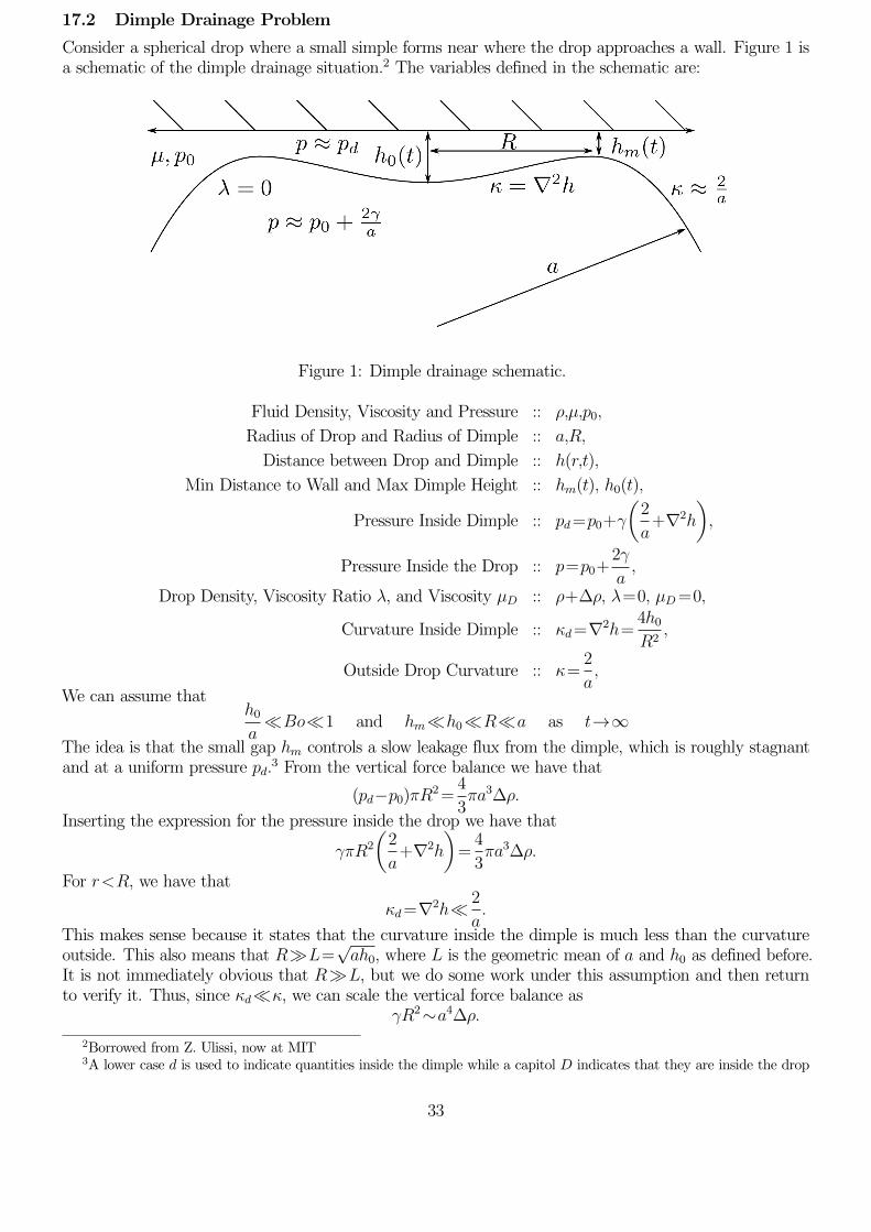
17.2 Dimple Drainage Problem

Consider a spherical drop where a small simple forms near where the drop approaches a wall. Figure 1 isa schematic of the dimple drainage situation.2 The variables defined in the schematic are:

1. High pressure in the gap will deform the drop by h over lengthscale L. The deformationcan be estimated

p

h

L2

h

h0 p

/a µh0

a2

h2

The deformation is small if the first term is small compared to h2/a2, and is called thecapillary number

µh0

Ca

h2

a2

Equivalently, the Bond number must also be small

Bo ga2

h

a

Either way, as h continues to decrease (the sphere falls), the deformation assumption willbreak down.

2. Shear stress against the bubble can drive circular flow over lengthscale L

The stress balance on the sphere will be

µu

h0 µuD

L) uD

u

a

h0

1/21

so that the rigid boundary condition u = 0 at z = h is ok if (a/h0)1/2, which will

eventually be invalid as well.

So, two extensions to the model are necessary to treat these two issues:

1. If (a/h0)1/2, we can neglect the shear stress exerted by the drop on the squeeze film

(the drop is essentially inviscid compared to the film). We then replace the boundarycondition at z = h by @u/@z = 0. h0/F increases by a factor of (1/3)/(1/12) = 4 so thatthe bubble falls four times as fast.

2. If Bo h/a, we get a dimple, which is a more complicated situation.

Example: Dimple Drainage between a Bubble and a Wall

32Figure 1: Dimple drainage schematic.

Fluid Density, Viscosity and Pressure :: ρ,µ,p0,

Radius of Drop and Radius of Dimple :: a,R,

Distance between Drop and Dimple :: h(r,t),

Min Distance to Wall and Max Dimple Height :: hm(t), h0(t),

Pressure Inside Dimple :: pd=p0+γ

(2

a+∇2h

),

Pressure Inside the Drop :: p=p0+2γ

a,

Drop Density, Viscosity Ratio λ, and Viscosity µD :: ρ+∆ρ, λ=0, µD=0,

Curvature Inside Dimple :: κd=∇2h=4h0R2

,

Outside Drop Curvature :: κ=2

a,

We can assume thath0aBo1 and hmh0Ra as t→∞

The idea is that the small gap hm controls a slow leakage flux from the dimple, which is roughly stagnantand at a uniform pressure pd.

3 From the vertical force balance we have that

(pd−p0)πR2=4

3πa3∆ρ.

Inserting the expression for the pressure inside the drop we have that

γπR2

(2

a+∇2h

)=

4

3πa3∆ρ.

For r<R, we have that

κd=∇2h 2

a.

This makes sense because it states that the curvature inside the dimple is much less than the curvatureoutside. This also means that RL=

√ah0, where L is the geometric mean of a and h0 as defined before.

It is not immediately obvious that RL, but we do some work under this assumption and then returnto verify it. Thus, since κdκ, we can scale the vertical force balance as

γR2∼a4∆ρ.2Borrowed from Z. Ulissi, now at MIT3A lower case d is used to indicate quantities inside the dimple while a capitol D indicates that they are inside the drop

33

Rearranging and invoking the definition of the Bond number (assuming Bo1) we have that

R∼a√Bo.

Inserting this back into the expression relating R and the geometric mean of a and h0 we have that

a√Bo

√ah0−→Bo h0

a,

where the right hand expression is one of assumptions and therefore we were justified in taking κdκ.Now we will examine the shape of the dimple. Because the pressure inside the dimple is uniform, we have that

∇2h=constant−→h=h0

(1− r2

R2

).

The volume trapped in the dimple isV ∼h0R2.

In the thin gap we have a free surface lubrication theory leakage flux of

q=h3

3µ

∂

∂x

(γ∂2h

∂x2

),

where x=r−R is a local coordinate. We also have that∂V

∂t=−2πRq−→ ∂h0

∂t∼q.

The boundary conditions are that∂h

∂x→ 2h0

R2as x→−∞

∂2h

∂x2→ 1

aas x→∞

Scaling these expressions we have thath

x∼ h0 :: No spatial dependence in h0

h4

x3∼ q∼ h

t:: Mass flux equations

h

x2∼ 1 :: From the divergence of h

Thus, by some simple algebra we can see that

h∼t−12 and x∼t−1

4 and q∼t−54 and h0∼t−

14 .

Thus, we expect a similarity solution of the form

ξ=x

Bt−14

and h=At−12H(ξ).

Inserting this into the flux condition we have thatH3H′′′=1 subject to H′→−1 as ξ→−∞.

We must be careful about counting with nonlinear boundary conditions, because the given boundary conditionis the same as H′′→0 as ξ→−∞. The unique solution, up to a choice of origin, is

H∼ 1

2Cξ2,

where the constant is found numerically. The remaining constants are determined from the unscaled condition

h∼ 1

2ax2 as x→∞.


18.1 Gravity Current on an Inclined Plane

Here we have a gravity current of fluid with density ρ and viscosity µ flowing down flat plane inclined at anangle θ. The x direction is aligned with the plane and down, the same direction that the current is flowing. Thecoordinate z is perpendicular to the plane. Because the coordinate system is rotated, gravity has componentsboth normal and parallel to the plane. Thus, from lubrication theory we can write the x momentum balance as

µ∂2u

∂z2=∇p·x−ρgsin(θ).

34

Here we consider ∇p to be a constant. It is important to note that there is a component of gravity parallelto the slope, but not across the slope. That is, there is no gravity component in the y direction. We alsohave that the pressure in the current is hydrostatic, thus,

p=p0+ρgcos(θ)(h−z).Therefore, we can integrate the x momentum equations twice and insert the pressure gradient, ∇p=ρg∇h=constant, whence we find that

u=−ρg2µ

cos(θ)∇h·x(2h−z2

)+ρg

2µsin(θ)

(2h−z2

).

Then, we can integrate this expression to give the depth-integrated flux vector as

q=− g

3νcos(θ)h3∇h+

g

3νsin(θ)h3x.

By mass conservation, we have that∂h

∂t+∇·q=0.

Thus, inserting we can see that

∂h

∂t+gsin(θ)

3ν

∂h3

∂x=gcos(θ)

3ν∇·(h3∇h

).

Taking the steady state of this equation for large distances downslope, hyNx, we can scale this equation to

tan(θ)∂h3

∂x=∂

∂y

(h3∂h

∂y

)−→ h3

x∼ h4

y2N. (35)

Considering a source of constant volume fluxQ, from the x component of the depth-integrated flux we have that

Q=

∫ h

0

∫ yN

−yNudydz=

∫ yN

−yNq·xdy.

This gives the flux through a sheet in the yz-plane. Scaling, with hx, we have thatQ∼h3yN .

Combining this with equation (35), we have that

x∼h−7 and yN∼h−3 and yN∼x37 .

From these scalings we find that the PDE in equation (35) admits a similarity solution. Starting with

h=x−17H(η) and η=

yN

x37

=yNx−3

7 ,

where the constants are omitted, we also have that∂

∂x=∂η

∂x

∂

∂η=−3

7

η

x

∂

∂ηand

∂

∂y=∂η

∂y

∂

∂η=x−

37∂

∂η.

Inserting these expressions into equation (35) we have that

−3x−37

7x

(H3+η3H2H′

)=x−

37

x

(H3H′

)′,

where the prime indicates a derivative with respect to η. The term on the left hand side can be made intoa total derivative, and by canceling x powers, we have

−3

7

(ηH3

)′=(H3H′

)′.

We can then integrate once. The constant of integration is zero because H=0 at η=±ηN . Thus,

−3

7ηH3=H3H′−→ ∂H

∂η=−3

7η.

This gives the familiar expression

H=3

14

(η2N−η2

).

The location of the nose can be determined from the flux condition:

Q=

∫ yN

−yNq·xdy' 1

3

∫ ηN

−ηNH3dη.

Plugging in the equation for H that we just determined and using the substitution ξ=η/ηN , and the integral∫ 1

−1(1−u2)3du=

32

35,

we have that

η7N =

(35·33·143

3·32

)−→ ηN =

(12005

36

)17

.

35

18.2 Axisymmetric Horizontal Gravity Current

Here we consider the axisymmetric flow of a viscous gravity current of density ρ0. The ambient fluid hasdensity ρ0−∆ρ. The radial coordinate is r, the height is h(r,t), and the position of the nose is rN(t). Locally,we consider the lubrication flow with

∇·u=0,

0=−1

ρ∇p+

µ

ρ∇2u−∆ρ

ρ0gz.

This is assuming a small Reynolds number, and therefore inertia can be neglected. The key observationis that horizontal lengthscales are much smaller than vertical lengthscales, as in

HL,

U∼ L

HWW.

The vertical component of momentum is hydrostatic as∂P

∂z=−∆ρg−→ P=P0∆ρg(h−z).

The radial pressure gradient is therefore∂P

∂r=∆ρg

∂h

∂r.

From the horizontal momentum equation, where the radial terms are neglected, we find that∆ρg

µρ0

∂h

∂r=∂2u

∂z2.

Integrating twice we find that

u(z)=−∆ρg

µρ0

∂h

∂r(2h−z)z,

where there is a stress free upper surface, i.e.,∂u

∂z

∣∣∣∣z=h

=0,

and there is no slip on the bottom surface (z=0). An important quantity in these flows is the depth integratedfluid flux, q, which is found by integrating the velocity field as

q=

∫ h

0

u(r,z,t) dz=∆ρg

3µρ0h3∂h

∂r.

Considering a slice of width δr, mass conservation can be written as

2πrδr∂h

∂t+2π(r+δr)q(r+δr)−2πrq(r)=0.

As the width of the slice decreases to zero, we are left with∂h

∂t+

1

r

∂

∂r(rq)=0.

Inserting the derived expression for q we find that∂h

∂t−∆ρg

3ρ0µ

1

r

∂

∂r

(rh3

∂h

∂r

)=0. (36)

To this point the derivation has been fairly general, now if the gravity current is considered to be a constantvolume, we have the additional condition that

V =2π

∫ rN

0

hr dr. (37)

As equation (36) is a nonlinear diffusion equation, it is reasonable to anticipate a similarity solution. Scalingequation (36) and the constant volume condition, equation (37) we can see that

h

t∼γh

4

r2,

V ∼hr2.Here the term γ is the combination of constants

γ=∆ρg

3ρ0µ.

Solving for h and r, we find that

h∼(V

γt

)14

,

36

r∼(γV 3t

)18 .

We can now define the similarity variable, η and the similarity shape function, f(η) as

η=r

(γV 3t)18

,

h=

(V

γt

)14

f(η).

Inserting these expressions into equation (36) and converting derivatives with respect to r to derivativeswith respect to η we find that

∂h

∂t=− 1

4t

(V

γt

)14

f(η)−(V

γt

)14 ∂f

∂η

η

8t,

and

−γr

∂

∂r

(rh3

∂h

∂r

)=−1

η

(V

γt5

)14 ∂

∂η

(ηf3

∂f

∂η

).

Combining the two expressions and setting the result equal to zero we find that

∂h

∂t−γr

∂

∂r

(rh3

∂h

∂r

)=− 1

4t

(V

γt

)14

f(η)−(V

γt

)14 ∂f

∂η

η

8t−1

η

(V

γt5

)14 ∂

∂η

(ηf3

∂f

∂η

)=0.

Thus, we can rearrange and cancel terms to find that

−η4f−∂f

∂η

η2

8=∂

∂η

(ηf3

∂f

∂η

).

The left hand side of this last equation is a total derivative and thus the whole expression can be rewritten as

−1

8

∂

∂η

(η2f)

=∂

∂η

(ηf3

∂f

∂η

).

Integrating once, using the fact that the slope of the height is zero at r=0, we find that

−η2

8f=ηf3

∂f

∂η.

This simplifies to

η=−8f2∂f

∂η,

which can be integrated again to yield1

2

(η2N−η2

)=8f3.

Here ηN is the position of the nose of the gravity current (and the constant of integration). Solving for theshape function we find that

f=

(1

16

(η2N−η2

))13

.

The position of the nose can be determined from the constant volume condition. Converting equation ??into similarity form we have

1=2π

∫ ηN

0

fη dη.

Inserting the derived similarity expressions we have

1=2π

∫ ηN

0

fη dη=2π

∫ ηN

0

(1

16

(η2N−η2

))13

η dη.

Integrating using a substitution for (η2N−η2), we find that(1

16

)13 3π

4η

83N =1.

Rearranging and solving for ηN we find that

ηN =

(1024

27π3

)18

,

and thus, the actual position of the nose is

rN =(γV 3t

)18ηN =

(1024

243π3∆ρgV 3t

ρ0µ

)18

.

37

18.3 Similarity Solutions

In looking for a similarity solution of a differential equation, we have two variables:

(1) F=Atαf(η) and (2) η=x

Btβ.

The two types of derivatives are then given as∂

∂x

(Atαf

( x

Btβ

))=

Atα

Btβf ′(η),

∂

∂x

(Atαf

( x

Btβ

))= Atα−1(αf−βηf ′)

Integral conditions are then given as ∫·dx=Btβ

∫·dη,

where · is the object operated on.

18.3.1 Diffusion from a Spherical Heat Pulse

A classic example of the application of similarity solutions is the problem of a fixed amount of heat beingrelease as an axisymmetric sphere. The equations are

∂T

∂t=κ

r2∂

∂r

(r2∂T

∂r

)and Q=4π

∫Tr2 dr.

Scaling we have thatT

t∼ κTr2

and Q∼Tr3,and thus, r∼

√κt, which is very typical for diffusion problems. This scaling motivates the choice of variables

T=Qt−32f(η) and η=

r√κt.

Inserting these into the equation we find that

−3

2f−η

2f ′=

1

η2(η2f ′

)′.

Bringing the η2 term to the other side, rearranging it into a total derivative, and integrating once we have

−1

2η3f=η2f+C.

The constant of integration is zero because f=0 as η→∞. Canceling terms and integrating again we find that

f=Ae−η2

4 .Applying the integral condition gives

1=4πA

∫ ∞

0

e−η2

4 η2 dη.

Using a change of variables and the gamma function,

Γ(α)=

∫ ∞

0

tα−1e−t dt,

we have that

A=1

16πΓ(32

)=1

(4π)32

.


19.1 Long Thin Flows II: Extensional Flow

Consider an axisymmetric thin flow with an effectively stress-free boundary. A viscous thread is falling undergravity. The radius of this thread is a(z) and it changes over the lengthscale L. The velocity in the threadis w(z,t). The coordinate system is z pointing down and r points out horizontally.

Similar to a lubrication theory approximation, here we can assume that

La→ ∂

∂r ∂

∂zas

1

a 1

L.

The stress free boundary condition on r=a gives that

µ∂w

∂r=0−→w=w(z,t).

The important thing about this boundary condition is that w is not a function of r and thus, we have plug flow.

38

We can derive mass conservation by thinking of a slice of fluid that is δz thick. The flowrate of fluid intothe slice is A(z)w(z) and the flow rate out is A(z+δz)w(z+δz). The change in area with time is given as∂A/∂t, thus, we can write mass conservation as

−δz∂A∂t

+A(z)w(z)−A(z+δz)w(z+δz)=0.

Thus, collapsing the slice to infinitesimally small, we ahve that∂A

∂t+∂

∂z(Aw)=0.

This implies thatDA

Dt=−A∂w

∂z,

where D/Dt is the total or Lagrangian derivative operator. Locally, the continuity equation gives

∇·u=1

r

∂

∂r

(ru)+∂w

∂z=0.

Because w is not a function of r we can integrate to find that

u=−1

2r∂w

∂z←→ ∂u

∂r=−1

2

∂w

∂z.

Now we can consider the radial and axial force balances:

1. Radial Stress:

σrr=−pext=−p+2µ∂u

∂r=−p−µ∂w

∂z,

where, pext is the external pressure. Thus,

p−pext=−∂w

∂z.

2. Axial Stress:

σzz=−p+2µ∂w

∂z=−pext+3µ

∂w

∂z

If we consider the same slice of fluid from before and now compute the force balance, because forces balancein Stokes flow, we have that

(A(z)σzz(z)−A(z+δz)σzz(z+δz))−δzpext∂A

∂z−δzAf=0.

The second last term is the external pressure force on the weakly slope sides of the slice and the last termis the axial body force. Thus, we have that

∂

∂z(Aσzz)+pext

∂A

∂z+Af=0.

Inserting the expression we found for σzz we have that∂

∂z

(−Apext+3µA

∂w

∂z

)+pext

∂A

∂z+Af=0.

Canceling one of the external pressure terms we can rewrite this equation as3µ

A

∂

∂z

(A∂w

∂z

)−∂pext

∂z+f=0.

Thus, the two important equations in extensional flows are:

∂A

∂t+∂

∂z(Aw)=0 or

DA

Dt= −A∂w

∂z, (38)

3µ

A

∂

∂z

(A∂w

∂z

)−∂pext

∂z+f = 0. (39)

Some variations to this solution are:

1. The external pressure pext might include a contribution from surface tension.

2. The unidirectional extension of a sheet has∂u

∂x=−∂w

∂zand A→h.

Trouton viscosity is 4µ rather than 3µ and in the general case there is coupling between u and v.

39

3. We could include inertia, as Dw/Dt. This would give a long-wave cut-off to the Rayleigh instabilitywith ak∼Oh−2 where Oh is the Ohnesorge number.

4. In this analysis we did not include the rapid response by bending, which gives rise to a lateral force.

Now we will consider two cases:

19.1.1 Steady Flow

Fluid flows out of a vertical orifice at a constant volume rate Q and extends due to gravity. From equations(38) and (39), we have that

Aw = Q.

w

Q

∂

∂z

(Q

w

∂w

∂z

)+g

3ν= 0.

Far from the nozzle, we can postulate a self-similar solution of the formw=γ(z−z0)α,

where α and γ are arbitrary constants. Inserting this into the force balance, the second equation, we find that

αγ(z−z0)α−2=g

3ν.

Thus, we find that

w=g

6ν(z−z0)2.

Thus, we can find how the area evolves as

A=Q

w→A=

6Qν

g(z−z0)−2

As a check we can see that this solution satisfies

A∂w

∂z→0 as z→∞,

as

A∂w

∂z=2Q(z−z0)−1→0 as z→∞.

In determining this solution we have assumed that the thread is slender. This assumption can be checkedby determining whether √

A

L1,

where L=z−z0. This condition reduces to

z−z0(

6Qν

g

)14

.

In this analysis we have also neglected inertia. Computing the Reynolds number as

Re=wL

ν,

allows us to determine whether viscosity or inertia dominates. Thus, to neglect inertia we needw(z−z0)

ν1⇐⇒ g(z−z0)3

6ν21.

Once the drop enters the inertia-dominant regime the predominant balance in the momentum equationsis between inertia and gravity. Thus,

ρw∂w

∂z∼ρg−→w∼

√2gz,

which is free fall. The transition between the viscous dominated regime and the inertia dominated regimeoccurs around

z∼(ν2

g

)13

,

from the Reynolds number condition.

40

19.1.2 Transient Evolution

Now we consider a fluid the ejected through a nozzle of area A0 with volume flux Q. This gives an initialvelocity of w0 =Q/A0. Thus, we can integrate the force balance, equation (39), and insert it into massconservation, equation (38). This gives

DA

Dt=− g

3ν

∫ L(t)

z

A(ς,t)dς=−A∂w∂z. (40)

Here L(t) is the length of the drip. This expression states that a material slice of fluid thins because ofthe weight of fluid hanging below it and so viscous stresses must support the fluid below. Thus, we canlabel slices by their original release time, t0. The bottom of the thread, at L, was released at time t0 =0.Subsequent times can be determined from ∫ L

z

A(ς,t) dς=Qt0.

This can be rewritten, due to volume conservation, as∂

∂z=−A

Q

∂

∂t0.

Furthermore, the total derivative in the mass conservation equation can be changed to a single derivativeevaluated at t0, that is,

D

Dt=d

dt

∣∣∣∣t0

.

Hence, using these three expressions we can rewrite mass conservation, equation (40), asdA

dt=−gQt0

3ν=A2

Q

∂w

∂t0.

Using the first two expression we have that∫ A

A0

dA′=−∫ t

t0

gQt03ν

dt′,

which gives

A=A0−gQ

3νt0(t−t0).

Thus, we can see that A=0, i.e., break-up, occurs when

t=t0+3νA0

gQt0.

This is minimized when∂t

∂t0=0−→1−3νA0

gQt20=0,

and therefore

tmin0 =

√3νA0

gQand tmin=2

√3νA0

gQ.

This shows that exactly half of the mass breaks off and the flow continues to evolve and periodically producesmore drops of equal size.

Now we can examine the vertical velocity. We do this by integrating over all of the slices from the oneof interest to the one currently being released. Starting with

w=w0+

∫ t0

t

∂w

∂dt′0dt′0,

we can insert the second relationship from the transient mass conservation as

w=Q

A0

+gQ2

3ν

∫ t

t0

t′0A2

dt′0.

Here the variable t′0 is the dummy variable for integration and in getting to the last expression the limitsof integration were switched, canceling a minus sign. This allows us to write that: the distance traveled byslice t0 between time of release and the current time is:

z=

∫ t

t0

w dt′

41

Now nondimensionalizing the equations, we have

Timescale :: τ=t

√gQ

3νA0

Velocity :: W=wA0

Q

Lengthscale :: ζ=z

√gA0

3νQ

Area :: A=A/A0

Thus, the equations become

A=1−τ0(τ−τ0), and W=1+

∫ τ

τ0

τ ′0A2

dτ ′0, and ζ=

∫ τ

τ0

W dτ ′.

Combining the expressions for the nondimensional area A and velocity W , we have that

W=1+

∫ τ

τ0

τ ′0(1−τ ′0(τ−τ ′0))2

dτ ′0.

Using Mathematica or otherwise, it can be shown that

ζ=2√

4−τ2arctan

(2(τ−τ0)

√4−τ2

τ(2τ0−τ)

).

Break-up time occurs when τ→2 and the breaking slice happens at τ0→1. Near τ→2, the expression inthe arctangent is small and therefore we can Taylor expand it to first order. Thus, we have that

ζ∼ 4(τ−τ0)τ(2τ0−τ)

.

Doing the same thing for the area expression and inserting the break-up time we have that

ζ∼ 2−τ0τ0−1

and A∼(1−τ0)2.Combining these expressions we find that

A∼ 1

(ζ+1)2.

Thus, the shape right before break-up is an inverse square. The steady solution near break-up also givesan inverse square,

Ast=2

(z−z0)2.


20.1 Long Thin Flows III: Two Fluid Case

Here we examine when boundary conditions are effectively rigid or when they are stress-free. The examplethat we will use is of a viscous gravity current spreading along the interface between two fluids, as in anoil slick spreading between water and air. Now let us imaging that the viscosity of the two fluids is matchedand equal to µ, while the viscosity of the inner fluid is λµ. Density of the upper layer is ρ1, the density of thebottom layer is ρ2, and the density of the middle layer is ρ0. At long times, the radius R of the gravity currentis much larger than the thickness at the center, H(t). We can also say that the thickness of the currentabove the interface, z=0, is h1 and the thickness below is h2. The radial and time dependent thicknessis h(r,t)=h1+h2. On all of these quantities, any influence of initial conditions has dissipated.

The vertical force balance is hydrostatic. Therefore,p=p0−ρ1gh1+ρ0g(h1−z)=p0+ρ2gh2−ρ0g(h2+z).

The first expression is starting from the top and working down, while the second expression starts from thebottom and works up. Combining the second two expressions we find that

(ρ0−ρ1)h1=(ρ2−ρ0)h2 with ρ1<ρ0<ρ2.Therefore, we can find out how much of the current is above the waterline and how much below. Now since thisis a long thin flow, the radial pressure gradient is computed as the derivative of the hydrostatic pressure. Thus,

∂p

∂r=(ρ0−ρ1)g

∂h1∂r

=(ρ2−ρ10)(ρ0−ρ1)

(ρ2−ρ1)g∂h

∂r=∆ρg

∂h

∂r,

42

where in this instance

∆ρ=(ρ2−ρ10)(ρ0−ρ1)

(ρ2−ρ1).

The rate of spreading of the current is determined by the resistance to motion. Scaling we have that thevelocity and volume conservation go as

u∼Rt

and V ∼R2H∼a3,where a is the initial radius of the spherical blob. From the radial force balance we have that the totalspreading force is given as the radial pressure gradient multiplied by the volume. Thus,

Fsp∼V∂p

∂r∼∆ρga3

H

R.

The viscous resistance, Fµ, is given by

Fµ∼µsuAsLs∼µs

R

tLsAs,

where µs and Ls are the viscosity and lengthscale that determine the dominant source of viscous resistance.As is the area over which is acts. Scaling the spread force, Fsp, with viscous resistance, Fµ, we have that

Fsp∼Fµ→∆ρga3H

R∼µs

R

tLsAs.

We can now define a dimensionless time τ , so that

T =∆ρgat

µ.

Rearranging the force balance and from volume conservation we have thatµsR

2Asµa2HLs

∼T andR2H

a3∼1.

If µs, Ls, andAs, are appropriately defined, we have two equations for the two unknownsR andH. Thus, thereare four possibilities based on the viscosity ratio λ, which will make its way into µs, and the aspect ratio R/H.

20.1.1 Toffee Stretch Regime

For large λ we have extensional flow and the dominant source of resistance is internal strain and

λ R

H.

The external fluid is effectively inviscid. The internal fluid is in plug flow and axisymmetric extension. Thisis the radial version of long thin flow. Thus, we have that

µs=λµ, Ls∼R, and As∼HR.This gives the scaling

R

a∼(Tλ

)12

.

20.1.2 Sliding Plate

When there is drag on the surfaces, external shear becomes the dominant source of resistance. Here we have thatH

Rλ R

H.

The internal flow is still approximately plug flow but is resisted by drag from the external fluid. There isa condition of matched shear stress at the interface. The external fluid sees the current as a disk of radialStokeslets, see integral representation. In this case, the parameters are

µs=µ, Ls∼R, and As∼R2.This yields

R

a∼T 1

5 .

43

20.2 Internal Shear

If we dial λ below H/R, we can no longer expect the velocity distribution to be uniform across the plug.The Poiseuille component of the internal flow is now larger than the velocity at which the external flow isdragged along. This is a lubrication flow and the internal shear gives a pipe flow, with

H

Rln(RH

)λH

R.

The relevant scalings areµs=λµ, Ls∼H, and As∼R2.

We then find that the current radius scales likeR

a∼(Tλ

)18

20.2.1 Nose Push

This regime is like a bubble, where the viscosity is very low, so that

λ H

Rln(RH

).Due to the low viscosity, the internal fluid can move along the current with negligible resistance but mustpush the external fluid out of the way at the nose. The external fluid sees the current as a ring with outforces, like slender body theory. Here we find that

µs=µ, Ls∼Hln

(R

H

), and As∼HR.

The radius ratio in terms of the timescale is thenR

aln(RH

)∼T 15 .


21.1 Pigs: Rigid Particle in a Tube

Consider a rigid tube with radius a, containing fluid of viscosity µ, and a tight-fitting axisymmetric, force-freeparticle. There is a constant applied pressure gradient

G∗=−∂p∂x.

Here the star indicates that the variable is dimensional. We would like to know what the steady speed U∗

of the bubble. Imagine tapioca balls in bubble tea.The radius of the tube is a and the gap thickness is εh. When the particle is fixed, the walls move

backwards. In the thin gap, there are two no slip conditions, one on the wall and one on the particle.Far from the particle we have Poiseuille flow. In the frame of the tube, the velocity is

u=G∗

4µ

(a2−r2

).

The volume flux is

Q∗=2π

∫ a

0

urdr=πa4G∗

8µ.

This gives an average velocity of

u=G∗a2

8µ.

In the thin gap we expect the velocity u to be less than the average velocity, as u<u. This means thatthe particle velocity U∗ is greater than the average velocity as U∗>u.

Now it is convenient to work in the frame of the particle, i.e. fix U∗ and find G∗, rather than vice versa.We can scale lengths with a, velocities with U∗, and pressures (as well as viscous stresses) with µU∗/a. Thus,

44

we have the equations∇2u = ∇p,∇·u = 0,

u = −x on r=1,

u = 0 on particle,∫

S

σ·n dA = 0 Force-free.

Here the x direction runs along the axis of the tube and the surface S is the surface of the particle. Weare looking for the pressure gradient

G=G∗a2

µu=Limx→±∞−

∂p

∂x.

Taking the fluid control volume so thatV =x1≤x≤x2, r≤1, outside particle,

and since Forces Balance in Stokes Flow we can write∫

S

σ·n dA+

∫

∂V

σ·n dA=0.

This simplifies to the new expression

π(p(x1)−p(x2))+2π

∫ (∂u

∂r+∂v

∂x

)∣∣∣∣r=1

dx=0.

Since the particle is force-free, there is no net force on it. Furthermore, the pressure gradient G and theflux Q through the gap must satisfy this force balance. In the region far away from the particle, we have

u=−1+G

4(1−r2) and Q=π

(G

8−1

)with

∂Q

∂x=0.

At the edge of the particle, the full Stokes equations apply. This is an order one region and the pressurevariations are order one as well. The details are irrelevant. In the intermediate region, outside the particleand far from the edges of the particle, the lengthscale L is order one, L=O(1). The lubrication scalings give

1−r=O(ε), u=O(1), Q∼uεh, and p∼ uL

(εh)2∼O(ε−2).

We can define a new coordinate

y=1−rε, for 0≤y≤h(x).

Then, using Poincare expansions, we can write the velocity, pressure, and flux asu = u0+εu1+...

p = ε−2p−2+ε−1p−1+...,

Q = εQ1+...The leading order expression is lubrication theory,

∂2u0∂y2

=∂p−2∂x

subject to u0(0)=−1, u(h)=0,

which integrates to

u0=y

h−1−1

2

∂p−2∂x

y(h−y).The flux can be calculated as

Q1

2π=

∫ h

0

u0 dy=−h2−h

3

12

∂p−2∂x

.

This equation can be rearranged to give

p−2(x1)−p−2(x2)=6

(Q1

π

∫

L

dx

h3−∫

L

dx

h2

).

From the force balance at order O(ε−2), we have thatπ(p−2(x1)−p−2(x2))=0.

This gives

Q1=−π∫Ldxh2∫

Ldxh3

.

45

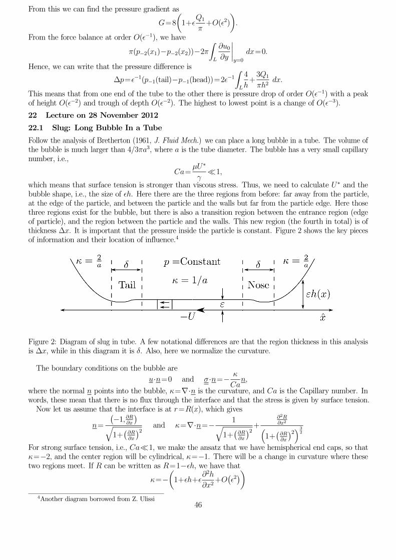
From this we can find the pressure gradient as

G=8

(1+ε

Q1

π+O(ε2)

).

From the force balance at order O(ε−1), we have

π(p−2(x1)−p−2(x2))−2π

∫

L

∂u0∂y

∣∣∣∣y=0

dx=0.

Hence, we can write that the pressure difference is

∆p=ε−1(p−1(tail)−p−1(head))=2ε−1∫

L

4

h+

3Q1

πh2dx.

This means that from one end of the tube to the other there is pressure drop of order O(ε−1) with a peakof height O(ε−2) and trough of depth O(ε−2). The highest to lowest point is a change of O(ε−3).


22.1 Slug: Long Bubble In a Tube

Follow the analysis of Bretherton (1961, J. Fluid Mech.) we can place a long bubble in a tube. The volume ofthe bubble is much larger than 4/3πa3, where a is the tube diameter. The bubble has a very small capillarynumber, i.e.,

Ca=µU∗

γ1,

which means that surface tension is stronger than viscous stress. Thus, we need to calculate U∗ and thebubble shape, i.e., the size of εh. Here there are the three regions from before: far away from the particle,at the edge of the particle, and between the particle and the walls but far from the particle edge. Here thosethree regions exist for the bubble, but there is also a transition region between the entrance region (edgeof particle), and the region between the particle and the walls. This new region (the fourth in total) is ofthickness ∆x. It is important that the pressure inside the particle is constant. Figure 2 shows the key piecesof information and their location of influence.4

Long Bubble in a Tube (Slug)

This problem was first considered by (Bretherton, JFM 1961). Consider a tube of radius acontaining fluid of viscosity µ and a large bubble of negligible viscosity. The bubble is big, inthat the volume is larger than 4/3a3.

Suppose that U is given and further that the capillary number is small (strong surface tension)

Ca µU

1

We wish to address two questions: the shape of the bubble and the pressure gradient. For thepig problem, the pressure gradient was

G =8µ

a2

U +

Q

a2

This result was independent of the details of the pig derived from the Stokes flow in the far field.We thus need to calculate Q and h(x). Because surface tension is strong (Ca 1), we take asan ansatz that the bubble has two hemispherical caps joined together by a cylinder. There willbe a jump in the curvature where these two caps meet.

Where is constant the pressure in the film is uniform, meaning that there is no pressure gradientand thus no driven flow (there will only be plug flow driven by the wall). This is true everywhereexcept in the nose and tail regions, where the curvature changes (from 1/ to 2/). We thenseek a scaling solution for the size of the nose and tail.

Width Change in Thickness "Change in Curvature 1

a "2

Thus, will scale like (a")1/2. The change in which drives a flow in the gap.

/a

µU

"2) " aCa2/3 a

aCa1/3 a

Shape of the nose:

37

Figure 2: Diagram of slug in tube. A few notational differences are that the region thickness in this analysisis ∆x, while in this diagram it is δ. Also, here we normalize the curvature.

The boundary conditions on the bubble are

u·n=0 and σ·n=− κ

Can,

where the normal n points into the bubble, κ=∇·n is the curvature, and Ca is the Capillary number. Inwords, these mean that there is no flux through the interface and that the stress is given by surface tension.

Now let us assume that the interface is at r=R(x), which gives

n=

(−1,∂R

∂x

)√

1+(∂R∂x

)2 and κ=∇·n=− 1√1+(∂R∂x

)2 +∂2R∂x2(

1+(∂R∂x

)2)32

For strong surface tension, i.e., Ca1, we make the ansatz that we have hemispherical end caps, so thatκ=−2, and the center region will be cylindrical, κ=−1. There will be a change in curvature where thesetwo regions meet. If R can be written as R=1−εh, we have that

κ=−(

1+εh+ε∂2h

∂x2+O(ε2))

4Another diagram borrowed from Z. Ulissi46

In the region of order εh between the bubble and the wall, where κ is constant, the pressure is uniformand there is no pressure gradient. Thus, the flow is driven as plug flow by the wall. This is true everywhereexcept in the nose and tail regions, the location where the curvature changes. The pressure drop acrossthe bubble is on the order of O(1/Ca). We can now scale the change in pressure and boundary conditions as

∆p

∆x∼ u

(εh)2, ε

∂2h

∂x2∼1, and ∆p∼ 1

Ca.

From these scalings we have that

ε∼Ca23 , ∆x∼Ca1

3 , and ∆p∼Ca−1.We can therefore define a new pressure P and the small scaling ε to be

P=∆pCa=(p−pbubble)Ca. and ε≡Ca23 .

In the region far from the bubble, we have uniform Poiseuille flow. This gives a flux of

Q=π

(G

8−1

),

where G is the dimensionless pressure gradient. At the edge of the bubble the full Stokes equations apply andthe deviatoric stresses are of order O(1). The pressure gradient∇P is on the order of the Capillary number, as

∇P=O(Ca)1−→P=constant.Thus, we can set the pressure equal to the curvature,

P=κ.At leading order P and κ are constant we have that

P0=κ0=−2.These are the hypothesized spherical end caps. In the center region, far from the end caps, we have, toleading order constant pressure and a cylindrical bubble. This gives

P0=κ0=−1.From lubrication theory, there is uniform flow, with a velocity and flux given by

u0=−1 andQ1

2π=−h0, where h0=uniform/constant.

22.1.1 Nose Region

Near the nose of the bubble, the curvature adjusts from the spherical end cap to the cylinder center. Thethickness of this region is ∆x∼Ca1

3 . We can define two coordinates as

y=1−rCa

23

and X=x−x0Ca

13

.

Starting with the curvature condition

κ=−1−εh−ε∂2h

∂x2,

since ε∂2h/∂X2εh, we have the pressure equation

P=−1−ε ∂2h

∂X2.

Velocity is given by lubrication theory as

u0=−1−1

2

dP0

dXy(2h−y).

Integrating with respect to y, we find the volume flux isQ1

2π=−h−h

3

3

dP0

dX.

The constant flux condition, Q1 =−2πh0, from before and taking the derivative of the pressure heightrelationship gives the equation

−h+h3

3

∂

∂X

(−1− ∂2h

∂X2

)=Q1

2π=−h0.

Rearranging and computing derivatives we have that1

3h3∂3h

∂X3=h−h0.

Now we will make a similarity change of variables so that

ξ=3

13X

h0and h=h0H(ξ).

47

This gives the Landau-Levich equation, which is

H3H′′′=H−1 subject to H→1 as ξ→−∞ and H′′→ h0

323

as ξ→∞.Making the substitution, H→1, with δH=H−1, we have that

(δH+1)3δH′′′=δH.We can then linearize this expression to

δH′′′=δH.This gives an exponential solution with the characteristic polynomial

r3=1→r=1, e2π3i, e−

2π3i.

Due to the condition that δH→0 as ξ→−∞, the oscillatory solutions must have zero amplitude. Thus,we have that

δH=Aeξ−ξ0→H=1+δH→ H=1+Aeξ−ξ0.This is a unique solution within a choice of origin. Numerically, it can be found that as ξ→∞,

H∼ 1

2Cξ2 with C=0.643.

Thus,

h0=323C=1.337 and εh∼1.337Ca

23 .

This region determines the flux of fluid that goes in the cylinder region.

22.1.2 Tail Region

Near the tail of the bubble, by a similar argument the Landau-Levich equation applies, but this time withdifferent boundary conditions. Thus,

H3H′′′=H−1 subject to H′′→ h0

323

as ξ→−∞ and H→1 as ξ→∞.Changing coordinates and linearizing we find the same equation

δH′′′=δH,with the same three solutions

r3=1→r=1, e2π3i, e−

2π3i.

However, now because δH→0 as ξ→∞, the positive exponential term cannot be used and we are left withthe oscillatory sinusoids. Thus, the solution for H is

H=1+eξ1−ξ

2 cos

[√3

2(ξ−ξ1+φ)

].

Here ξ1 is the constant offset parameter. The phase φ is determined from the conditionH′′=C with C=0.643.

48

slow viscous flows lecture notespeople.seas.harvard.edu/~colinrmeyer/slow viscous flows...

Documents