a high performance dual revised simplex solver · a high performance dual revised simplex solver...

A high performance dual revised simplex solver

Julian Hall, Qi Huangfu and Edmund Smith

School of Mathematics

University of Edinburgh

2nd December 2010

A high performance dual revised simplex solver

Overview

• LP problems and the dual simplex method

• Why use dual simplex method

• Why exploit parallelism

• Dual revised simplex with suboptimization

• Preliminary results

• Alternative product form update for GPU extension

• Conclusions

A high performance dual revised simplex solver1

Linear programming (LP)

minimize f = cTx

subject to Ax = b x ≥ 0

• Fundamental model in optimal decision-making

• Solution techniques

◦ Simplex method (1947)

◦ Interior point methods (1984–date)

• Large problems have

◦ 103–107 variables

◦ 103–107 constraints

• Matrix A is (usually) sparse

STAIR: 356 rows, 467 columns and 3856 nonzeros


Mathematics of LP

minimize f = cTx

subject to Ax = b x ≥ 0(P )

• Geometry:

◦ Feasible points form a convex polyhedron

• Results:

◦ An optimal solution occurs at a vertex

◦ At a vertex the variable set can be partitioned as B ∪ N and constraints as

BxB +NxN = b

so B is nonsingular and xN = 0• Dual LP problem:

maximize f = bTy

subject to ATy + s = c s ≥ 0(D)

• Result:

◦ Optimal partition B ∪ N for (P ) also solves (D)


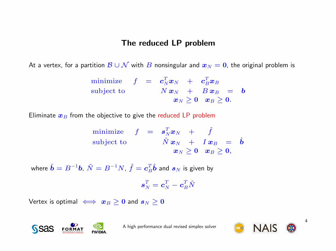
The reduced LP problem

At a vertex, for a partition B ∪ N with B nonsingular and xN = 0, the original problem is

minimize f = cTNxN + cTBxB

subject to N xN + B xB = b

xN ≥ 0 xB ≥ 0.

Eliminate xB from the objective to give the reduced LP problem

minimize f = sTNxN + f

subject to N xN + I xB = b

xN ≥ 0 xB ≥ 0,

where b = B−1b, N = B−1N , f = cTBb and sN is given by

sTN = c

TN − c

TBN

Vertex is optimal ⇐⇒ xB ≥ 0 and sN ≥ 0


Primal vs dual simplex

Finding an optimal partition B ∪ N underpins the simplex method

• Primal simplex method

◦ Maintains xB ≥ 0◦ Moves along edges of the feasible region of (P )

◦ Terminates when sN ≥ 0

• Dual simplex method

◦ Maintains sN ≥ 0◦ Moves along edges of the feasible region of (D)

◦ Terminates when xB ≥ 0

• Adaptations of both are required to find initial feasible point


Implementation: dual standard simplex method

N B RHS

1... N I b

m

0 sTN 0T −f

In each iteration:

• Choose a row p with bp < 0

• Use the pivotal row p of N and sN to find the pivotal column q with β = sq/apq

• Exchange indices p and q between B and N• Update tableau corresponding to this basis change

N := N − (1/apq)aqaTp b := b− (bp/apq)aq

sTN := sTN − βaTp −f := −f − βbp


Implementation: dual revised simplex method

• Maintains a representation of B−1 (rather than explicit N)

• Rows and columns of N obtained as required

• Pivotal row is

aTp = πTpN , where πTp = eTpB−1

• Pivotal column is

aq = B−1aq, where aq is column q of A

• Representation of B−1 is updated by exploiting

B := B + (aq − ap)eTp• Periodically a representation of B−1 is formed from scratch

• Efficient solution of large sparse LP problems requires the revised simplex method


Implementation: representing B−1

• Factorize some basis matrix B0 = L0U0

Store non-trivial columns of L0 and U0 as representation of B−10

• Updating representation of B−1 each iteration exploits

B := B + (aq − ap)eTp= B[I + B−1(aq − ap)eTp ]= B[I + (aq − ep)eTp ]

where aq is the pivotal column so, using Sherman-Morrison and apq = eTp aq,

B−1k =

[I − (aq−ep)eTp

apq

]B−1k−1= E−1

k B−1k−1

• Hence

B−1k = H−1

k B−10 where H−1

k = E−1k . . . E−1

1


Summary: major computational components for simplex implementations

Standard simplex method (SSM)

• Update tableau N := N − (1/apq)aqaTp

Revised simplex method (RSM)

• Operations

◦ Form πTp = eTpB−1

◦ Form aTp = πTpN

◦ Form aq = B−1aq

• Inversion of B

• Distinctive features

◦ Vectors ep, aq are always sparse

◦ B may be highly reducible

◦ B−1 may be sparse

◦ Vectors πp, ap and aq may be sparse

• Efficient implementations must exploit these features

H and McKinnon (1998–2005)


Why use the dual simplex method?

• Dual simplex method has been around almost as long as the primal simplex method

• More of theoretical interest until 1990’s

• Now preferred to primal simplex

◦ Easier to find feasible point of (D) to start

◦ Has some efficient algorithmic tricks not available to primal

◦ Dual feasibility retained when constraints are added (MIP)

• Primal simplex method applied to (D) can be made computationally equivalent


CPLEX LP solvers applied to standard test problems

• Dual simplex better than primal but barrier clearly better


CPLEX LP solvers applied to standard test problems

• Little to choose between dual simplex and barrier with crossover


Parallel simplex: why?

• Moore’s law drives core counts per processor, but clock speeds will stabilise

• Serial performance of simplex is spectacularly good

◦ Flop count per iteration is near optimal

◦ Number of iterations is near optimal

• Can’t wait for faster serial processors or algorithmic improvement

• Simplex method must try to exploit parallelism


Parallel simplex: immediate scope

• Standard simplex method

◦ Update tableau N := N − (1/apq)aqaTp

Level 2 BLAS with N dense so “massively parallel”

• Revised simplex method

◦ Operations πTp = eTpB−1 and aq = B−1aq are “inherently serial”

◦ Operation aTp = πTpN is “massively parallel”

Amdahl’s law implies little immediate scope for exploiting parallelism


Parallel simplex: nature of B−10 and H−1

Properties of B−10 and H−1 are a majr influence on parallel schemes

• B−10 requires many vectors but they are short O(1)

◦ Parallelism is fine grained

◦ Unsuitable for data parallelism

◦ Aim for task parallelism

• H−1 requires few vectors but they are long O(m)

◦ Operations with H−1 can be posed as a sparse matrix-vector product

◦ Suitable for data parallelism


Parallel simplex: past work

• Data parallel standard simplex method

◦ Good parallel efficiency was achieved

◦ Totally uncompetitive with serial revised simplex method without prohibitive resources

• Data parallel revised simplex method

◦ Only immediate parallelism is in forming πTpN

◦ When n� m, cost of πTpN dominates: significant speed-up was achieved

Bixby and Martin (2000)

• Task parallel revised simplex method

◦ Overlap computational components for different iterations

Wunderling (1996), H and McKinnon (1995-2005)

◦ Modest speed-up was achieved on general sparse LP problems

• All data and task parallel implementations compromised by serial inversion of B

Review: H (2010)


Architectures: CPU or GPU or both?

Heterogeneous desk-top architectures

CPU:

• Fewer, faster cores

• Relatively slow memory transfer

• Welcomes algorithmically complex code

• Full range of development tools

GPU:

• More, slower cores

• Relatively fast memory transfer

• Global communication is expensive/difficult

• Very limited development tools

CPU and GPU:

• Possibly combine CPU and GPU to harness full computing power


Scope for task and data parallelism via suboptimization

• Perform multiple pricing—standard simplex suboptimization

◦ Primal: Orchard-Hays (1968)

◦ Dual: Rosander (1975)

• Algorithmically

◦ Primal: Identify attractive column slice of tableau

◦ Dual: Identify attractive row slice of tableau

◦ Both perform standard simplex iterations to identify a set of basis changes

• Computationally

◦ Solve systems with multiple RHS

◦ Update tableaux

◦ Form matrix products with multiple vectors

• Attractive in the days when memory access was expensive...

Primal: Parallel implementations by Wunderling (1996), H and McKinnon (1995-2005)

Dual: New, even in serial?


Dual revised simplex method with suboptimization

Let the current basis be Bk

• Choose attractive row set P• Form rows P of B−1

k : πTP = eTPB−1k

• Form rows P of tableau: aTP = πTPNk

• Perform l dual standard simplex iterations on aTP to identify column set Q• Form pivotal columns for q ∈ Q: aQ = B−1

k aQ

• Use aQ to update bk and H−1k to obtain bk+l and representation of B−1

k+l


Parallel operations with B−1k

• Consider operations with B−1k = H−1

k B−10 in stages corresponding to B0 and Hk

• Form πTP = eTPB−1k as

πTP = e

TPH

−1k

then

πTP = π

TPB−10

• Form aQ = B−1k aQ as

aQ = B−10 aQ

then

aQ = H−1k aQ


Gantt chart of computation and data

Operation with aTP Operation with aQ Operation with bk

Operation with H−1k Operation with B−1

0 Operation with Nk

bk+lH−1k+lH−1

k aQB−10 aQDual SSMπT

PNk

Invert Bk+lInvert Bk

πTPB−1

0eTPH−1

kP

• Inversion of Bk can take a whole major iteration...

◦ ... but not longer—for reasons of numerical stability

◦ Serial inversion could lead to load imbalance

◦ Inversion could be parallel?


Prototype implementation

• Written by Qi Huangfu (2010)

• Uses (generally) highly efficient core routines

Hyper-sparse matrix-vector product πTPNk

Dual steepest edge pricing

• Does not (yet) use

Hyper-sparse operations with B−1

Bound-flipping ratio test

• Written in C++ with OpenMP using the Intel C++ compiler

• Tested on a dual quad-core AMD Opteron 2378 system

• Uses one pivotal row per core used

• First run last week!


Preliminary results

pds-06: 9882 rows, 28655 columns and 82269 nonzeros

Cores

1 2 4 8 clp dual

Major iterations 10266 5049 2543 1253 9808

Total iterations 10266 9625 8820 7616 9808

Solution time (s) 3.76 2.51 2.00 1.52 1.92

Speed (iter/s) 2730 3836 4419 5017 5111


Preliminary results

pds-10: 16559 rows, 48763 columns and 140063 nonzeros

Cores

1 2 4 8 clp dual

Major iterations 17983 9158 4807 2557 17713

Total iterations 17983 17051 16263 15404 17713

Solution time (s) 12.58 10.01 6.86 5.72 6.61

Speed (iter/s) 1430 1704 2370 2695 2682


Can the simplex method exploit a GPU?

• Standard simplex method implemented in single precision by Smith as i8

• Experiments on machine with two quad-core AMD CPUs and GTX285 NVIDIA GPU

• For dense LP problems: best results

Solver Type HPC Time Iterations Speed (iter/s)

gurobi primal RSM serial 1357 16034 12

gurobi dual RSM serial 976 14518 15

i6 primal SSM parallel 4039 288419 79

i8 primal SSM GPU 800 221157 276

• Not (really) of practical value but a good learning exercise

• No hope of beating serial solvers on sparse LP problems

• Now adding steepest edge and extending to double precision for Tesla C2070


GPU extension

• Put dual standard simplex iterations on a GPU

• Consider putting other simple “rectangular” operations on a GPU

◦ Sparse matrix-vector product πTPNk

GPU out-performs comparable CPU for full vector (eg) Vuduc et al. (2010)

Nvidia interested in case of sparse vector

◦ Operations with H−1k

Can be posed as a sparse matrix-vector product

• Need to limit data transfer between main memory and GPU


Splitting work between CPU and GPU

GPU

CPU



0 Operation with Nk

bk+l

H−1k+lH−1

k aQ

B−10 aQ

Dual SSM


πTPNk

πTPB−1

0

eTPH−1

k

P

• CPU and GPU operations can be overlapped

• Data traffic between main memory and GPU is high


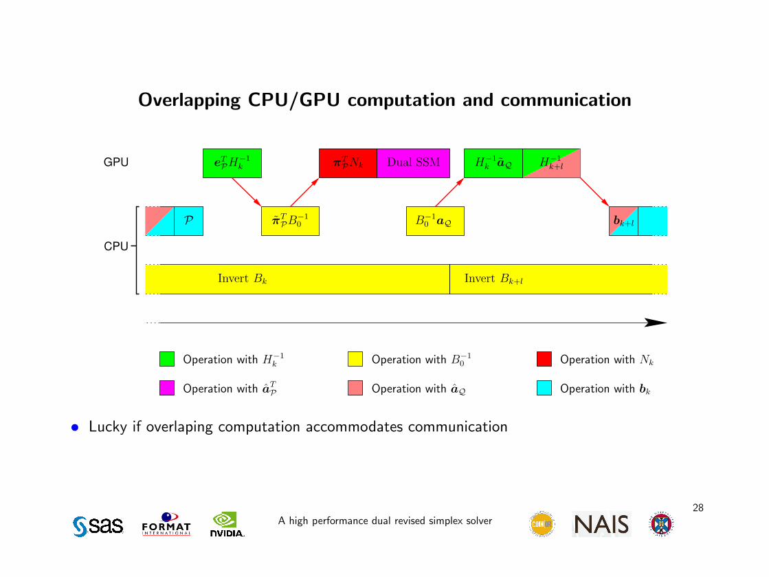
Overlapping CPU/GPU computation and communication

GPU

CPU



0 Operation with Nk

bk+l

H−1k+lH−1

k aQ

B−10 aQ

Dual SSMπTPNk


πTPB−1

0

eTPH−1

k

P

• Lucky if overlaping computation accommodates communication


Alternative product form update

• Little-known (unknown?) alternative product form update may offer a solution

• Updating representation of B−1 each iteration exploits

B := B + (aq − ap)eTp= [I + (aq − ap)eTpB

−1]B

= [I + (aq − ap)πTp ]B

so, using Sherman-Morrison,

B−1k = B

−1k−1

[I −

(aq − ap)πTpapq

]= B

−1k−1E

−1k

• Hence reversed the order of inverse and update in representation of B−1k

B−1k = B−1

0 H−1k where H−1

k = E−11 . . . E−1

k


Alternative dual revised simplex method with suboptimization

• Parallel operations with B−1k = B−1

0 H−1k

• Form πTP = eTPB−1k as

πTP = e

TPB−10

then

πTP = π

TPH

−1k

• Form aQ = B−1k aQ as

aQ = H−1k aQ

then

aQ = B−10 aQ


Splitting work between CPU and GPU

GPU

CPU



0 Operation with Nk

bk+l

H−1k+lH−1

k aQ

B−10 aQ

Dual SSM

Invert Bk+l

πTPNk

eTPB−1

0

πTPH−1

k

P

• Data traffic between main memory and GPU is lower

• Shorter time for inversion of Bk+l


Overlapping CPU/GPU computation and communication

GPU

CPU



0 Operation with Nk

bk+l

H−1k+lH−1

k aQ

B−10 aQ

Dual SSM

Invert Bk+l

πTPNk

eTPB−1

0 eTPB−1

0

πTPH−1

k

P P

• Greater scope for overlapping computation

• Implementation will be very difficult


Conclusions

• Identified need for simplex method to exploit parallelism

• Developed prototype high performance dual revised simplex solver

• Initial results are encouraging

• Shown that the standard simplex method will run fast on a GPU

• Standard approach to linear algebra bad for CPU-GPU combination

• Alternative product form update may offer a solution


References

[1] R. E. Bixby and A. Martin. Parallelizing the dual simplex method. INFORMS Journal on

Computing, 12:45–56, 2000.

[2] J. A. J. Hall. Towards a practical parallelisation of the simplex method. Computational

Management Science, 7(2):139–170, 2010.

[3] J. A. J. Hall and K. I. M. McKinnon. PARSMI, a parallel revised simplex algorithm

incorporating minor iterations and Devex pricing. In J. Wasniewski, J. Dongarra, K. Madsen,

and D. Olesen, editors, Applied Parallel Computing, volume 1184 of Lecture Notes in Computer

Science, pages 67–76. Springer, 1996.

[4] J. A. J. Hall and K. I. M. McKinnon. ASYNPLEX, an asynchronous parallel revised simplex

method algorithm. Annals of Operations Research, 81:27–49, 1998.

[5] J. A. J. Hall and K. I. M. McKinnon. Hyper-sparsity in the revised simplex method and how

to exploit it. Computational Optimization and Applications, 32(3):259–283, December 2005.

[6] W. Orchard-Hays. Advanced Linear programming computing techniques. McGraw-Hill, New

York, 1968.


[7] R. R. Rosander. Multiple pricing and suboptimization in dual linear programming algorithms.

Mathematical Programming Study, 4:108–117, 1975.

[8] R. Vuduc, A. Chandramowlishwarany, J. Choi, M. Guney, and A. Shringarpurez. On the limits

of GPU acceleration. Not known, 2010.

[9] R. Wunderling. Paralleler und objektorientierter simplex. Technical Report TR-96-09, Konrad-

Zuse-Zentrum fur Informationstechnik Berlin, 1996.


a high performance dual revised simplex solver · a high performance dual revised simplex solver...

Documents